External Financing and the Role of Financial Frictions over the Business Cycle: Measurement and Theory * Ali Shourideh Wharton [email protected]Ariel Zetlin-Jones CMU [email protected]December 31, 2012 Abstract We examine the quantitative importance of financial market shocks in accounting for business cycle fluctuations. We emphasize the role financial markets play in real- locating funds from cash-rich, low productivity firms to cash-poor, high productivity firms. Using evidence on financial flows at the firm level, we find that for publicly traded firms (in Compustat), almost all investment is financed internally. However, using an alternative data source (Amadeus), we find that most investment by privately held firms is financed via external funds. Motivated by these observations, we build a quantitative model featuring publicly and privately held firms that face collateral con- straints and idiosyncratic risk over productivity as well as non-financial linkages. In our calibrated model, we find that a shock to the collateral constraints which generates a one standard deviation decline in the debt-to-asset ratio leads to a 0.5% decline in aggregate output on impact, roughly comparable to the effect of a one standard devi- ation shock to aggregate productivity in a standard real business cycle model. In this sense, we find that disturbances in financial markets are a promising source of business cycle fluctuations when non-financial linkages across firms are sufficiently strong. * We are indebted to V.V. Chari and Larry Jones for valuable advice. We would also like to thank Patrick Kehoe, Narayana Kocherlakota, Ellen McGrattan, Chris Phelan, Warren Weber, the Chari-Jones work- shop, especially Alessandro Dovis and Erick Sager, and seminar participants at Carnegie Mellon, UChicago, Chicago Booth, Columbia GSB, Kellogg, UPenn and the 2012 SED for helpful comments. Shourideh would like to thank NYU for their hospitality. Zetlin-Jones is grateful to the Bilinski Education Foundation and the National Science Foundation for support. 1
Transcript
External Financing and the Role of Financial Frictions
We examine the quantitative importance of financial market shocks in accounting
for business cycle fluctuations. We emphasize the role financial markets play in real-
locating funds from cash-rich, low productivity firms to cash-poor, high productivity
firms. Using evidence on financial flows at the firm level, we find that for publicly
traded firms (in Compustat), almost all investment is financed internally. However,
using an alternative data source (Amadeus), we find that most investment by privately
held firms is financed via external funds. Motivated by these observations, we build a
quantitative model featuring publicly and privately held firms that face collateral con-
straints and idiosyncratic risk over productivity as well as non-financial linkages. In
our calibrated model, we find that a shock to the collateral constraints which generates
a one standard deviation decline in the debt-to-asset ratio leads to a 0.5% decline in
aggregate output on impact, roughly comparable to the effect of a one standard devi-
ation shock to aggregate productivity in a standard real business cycle model. In this
sense, we find that disturbances in financial markets are a promising source of business
cycle fluctuations when non-financial linkages across firms are sufficiently strong.
∗We are indebted to V.V. Chari and Larry Jones for valuable advice. We would also like to thank PatrickKehoe, Narayana Kocherlakota, Ellen McGrattan, Chris Phelan, Warren Weber, the Chari-Jones work-shop, especially Alessandro Dovis and Erick Sager, and seminar participants at Carnegie Mellon, UChicago,Chicago Booth, Columbia GSB, Kellogg, UPenn and the 2012 SED for helpful comments. Shourideh wouldlike to thank NYU for their hospitality. Zetlin-Jones is grateful to the Bilinski Education Foundation andthe National Science Foundation for support.
1
1 Introduction
One role of financial markets is to reallocate capital from cash-rich, low productivity firms
to cash-poor, high productivity firms. In this paper, we examine the importance of shocks
to the ability of financial markets to reallocate capital for the magnitude and duration of
business cycles. In particular, we focus on the role of financial markets in funding investment.
In the aggregate, data from the flow of funds shows that internal funds generated by firms is
more than adequate to finance investment. This observation might lead an observer to think
disruptions in financial markets would have very modest business cycle effects. We argue,
however, looking only at the aggregates may be misleading. New evidence on privately held
firms (in the Amadeus data set) shows that almost all of investment by such firms is financed
via external funds. This data suggests that disruptions to the reallocative role of financial
markets could have a large impact on the investment and output of privately held firms and,
through spillovers on other firms, on aggregate economic activity. The size of the impact
depends critically both on the sensitivity of investment and output of privately held firms to
shocks to financial markets and on the extent to which there are spillovers from the actions
of privately held firms to the investment and output decisions of publicly held firms.
To analyze the quantitative importance of financial market shocks, we develop a model
in which firms are subject to idiosyncratic shocks so that it is desirable to reallocate capital
from low productivity firms to high productivity firms, but financial frictions impede this
reallocation. We model these frictions as collateral constraints and disturbances in the ability
of financial markets to reallocate capital as shocks to collateral constraints. Our approach
follows a substantial literature that has examined the role of financial market frictions over
the business cycle (see Bernanke et al. (1999), Kiyotaki and Moore (2008), and Jermann
and Quadrini (2011) to cite just three examples). We discipline our quantitative exercise by
using data on financial flows.
Our model differs from those in the existing literature by incorporating three key ingredi-
ents. First, data on financial flows shows that at the aggregate level, firms generate internal
funds substantially in excess of what they need to finance operations and investments. Thus,
if financial market frictions affect investment over the business cycle, they must affect the
reallocation of funds among firms rather than impeding the ability of firms to obtain invest-
ment funds from households. To allow for reallocation problems among firms, our model
features heterogeneous firms in the sense that each individual firm faces idiosyncratic risk
and incomplete markets.
Second, the evidence from Compustat shows that for publicly traded firms, almost all
capital expenditures can be financed using internal funds. We show, however, that the bulk
2
of capital expenditures by privately held firms is financed via external funds. To be consistent
with this large observed difference between the two types of firms in the data, our model
features both publicly held and privately held firms, each of which face potentially binding
collateral constraints. The difference between these types of firms is that publicly held firms
are owned by households that can better insure themselves against the idiosyncratic risk
affecting a particular firm than can owners of privately held firms.
Third, a key feature of the data is that firms use intermediate goods produced by other
firms as well as capital and labor to produce gross output. This observation implies that firms
are naturally connected with each other through trade linkages. We model these connections
by assuming that each firm in our model has a monopoly in producing a differentiated good
and uses the goods produced by other firms as an intermediate good in production. We show
that under reasonable parameter assumptions regarding the fraction of gross output that
represents use of intermediate goods and on the size of markups, these linkages across firms
can generate co-movement of output by publicly held and privately held firms in response
to financial market shocks. These linkages also play an important role in amplifying the
quantitative effects of financial shocks.
In our calibrated model, we find that a shock to the collateral constraints which generates
a one standard deviation decline in the aggregate debt-to-asset ratio leads to a 0.5% decline
in aggregate output on impact. This decline is roughly comparable to the effect of a one
standard deviation shock to aggregate productivity in a standard real business cycle model.
A collateral constraint shock also leads to a sizable decline in consumption, investment and
employment. We also find that shocks to collateral constraints induce persistent effects on
aggregates. In this sense, we find that disturbances in financial markets are a promising
source of business cycle fluctuations.
Firm heterogeneity plays a central role in generating our results. In our model firms
face idiosyncratic shocks to productivity and collateral constraints in accumulating capital.
We argue that a representative firm version of our model in which the collateral constraint
binds is inconsistent with aggregate data on financial flows in both the United States and
Europe. Specifically, in both the U.S. and the U.K., after paying for interest, taxes, pay-
ments to labor and other businesses for materials, the non-financial business sector in the
aggregate generates funds, which we call Available Funds, substantially in excess of funds
used for investment. This observation implies that it is difficult for macroeconomic models
with a representative firm subject to collateral constraints to produce large fluctuations in
investment and output in response to a tightening of collateral constraints. One reason is
that shareholders of firms have strong incentives to accept delayed payments in dividends so
as to relax current collateral constraints.
3
Our quantitative results are disciplined by data on firm level use of external funds for
investment. Disaggregated data on publicly held firms in the U.S. and the U.K. and on
privately held firms in the U.K. suggests that it is important to distinguish between these
subsets of firms. We develop a statistic to measure how much a subset of firms rely on
external financing. In particular, our statistic measures the amount of external funds used
for investment by firms. We find that in both the U.S. and the U.K., on average (over time)
roughly 20% of investment by publicly held firms is externally financed so that 80 % of
investment by firms is finaced by available funds. In the U.K., on average roughly 90% of
investment by privately held firms is externally financed so that only 10% of investment is
financed by available funds.
This observation motivates us to introduce a second type of heterogeneity in our model.
Specifically, we partition firms into those that are owned by diversified households, and
therefore better able to insure themselves against idiosyncratic risk and those that are owned
by entrepreneurs who cannot insure themselves against idiosyncratic risk. The observation
that privately held firms use external funds for investment to a much greater extent than do
publicly held firms suggests that the role played by financial markets in reallocating capital
for investment is more important for privately held firms than it is for publicly held firms.
In this sense, privately held firms are more likely to be affected by disturbances to their
collateral constraints than are publicly traded firms.
In our model, collateral constraints are present for both types of firms. Both public and
private firms can borrow up to a level proportional to their asset holding. Both types of firms
are limited in their access to financial markets, in the sense that they must borrow using
debt. We assume that, in addition to productivity risk, firms are subject to bankruptcy risk
so that the effective discount rate is higher than the interest rate for privately held firms.
However, because publicly held firms are owned by diversified households, the bankruptcy
risk does not raise the effective discount rate of publicly held firms. These differences in
effective discount factors imply that, in a stationary equilibrium, publicly held firms have
sufficient asset holdings so that the collateral constraint does not bind, whereas privately held
firms face occasionally binding constraints. The differences in the extent to which collateral
constraints bind implies that privately held firms are much more reliant on external funds
for investment than are publicly held firms.
Trade linkages across firms ensure that output and investment of different types of firms
move together. We assume that each firm, both public and private, produces a differentiated
good and there is monopolistic competition between different firms a la Dixit-Stiglitz. More-
over, we assume that each firm uses a bundle of goods produced by other firms as an input
as well as capital and labor. These elements capture observed markups and the observation
4
that gross output is roughly twice as large as value added.
In our quantitative model, under our assumed parameter values, a tightening of collateral
constraints lead to a decline in output. The economic mechanism that drives this result is
that for privately held firms a tightening of the collateral constraint decreases the demand
for capital by firms for whom the collateral constraint binds. For such firms, the decrease in
capital demand leads to a decrease in demand both for labor and for intermediate goods to
be used in production. As a result, the rental rate of capital and the wage rate both decline,
tending to raise the output of unconstrained firms. However, the fall in the wage and capital
rental rate results in a negative wealth shock to households and privately held firms, causing
a decline in demand for the final good – both for consumption and as an intermediate
input in production. Because goods are not perfect substitutes, demand for goods produced
by all firms falls, tending to lower output of unconstrained firms. Thus, a tightening of
collateral constraints has competing effects on the production of firms for whom the collateral
constraint does not bind. The effect of the shock on aggregate demand and intermediate
good production provide incentives for unconstrained firms to decrease production while the
effect of the shock on wages and interest rates provide incentives for unconstrained firms
to increase production. We show that under our reasonable parameter assumptions, the
aggregate demand and intermediate good effects dominate so that a tightening of collateral
constraints leads unconstrained firms to decrease their production.
We calibrate our quantitative model with both publicly and privately firms to be con-
sistent with four key facts from the financial flows data. We require the model to replicate
the share of gross output accounted for by privately held firms, the aggregate debt-to-total
assets ratio for all firms, the dispersion of the firm level debt-to-total assets ratio among
privately held firms, and the amount of external funds used for investment by privately held
firms. We show that these facts in the data help determine the quantitative importance of
disturbances to the collateral constraints in the model.
We then perform an impulse response analysis from the steady state of our calibrated
model. Specifically, we shock the economy with a partially persistent disturbance to the
collateral constraint which generates a one standard deviation decline in the debt-to-total
assets ratio of privately held firms on impact. We find that such an impulse generates a
0.5% decline in aggregate output on impact. Although sales of publicly held firms initially
rise on impact, partially off-setting the initial decline in sales by privately held firms, within
two periods they fall below the steady state level. The non-financial linkages we introduce
play an important role, both in dampening the initial response of publicly held firms and in
generating co-movement in sales after the second period of the shock.
Related Literature. Our paper is related to an extensive literature on the effect of
5
financial frictions in macroeconomics, starting from Bernanke and Gertler (1989), Carlstrom
and Fuerst (1997), Kiyotaki and Moore (1997), Bernanke et al. (1999) and more recently
Kiyotaki and Moore (2008) and Jermann and Quadrini (2011). The common goal is to
identify and understand the channels through which financial market disruptions affect eco-
nomic activity and their quantitative importance. Our goal in this paper is the same while
our approach differs in that we use data on external financing to discipline the importance
of these channels.
Our empirical work on external financing needs is related to a literature in corporate
finance which attempts to identify the extent to which firms face constraints in financing
their investment (see Fazzari et al. (1988), and Gilchrist and Himmelberg (1995) among
many others).1 The approach in this literature is to test the implications of models with
financing constraints, namely that Tobin’s Q as well as cash-flow would have a significant
effect on investment. Our approach, however, differs from theirs in that our measurement
approach emphasizes the role of financial markets in firms’ financing decision, i.e., how much
of their investment is financed using external funds. In this regard, our approach is closer
to the one taken by Rajan and Zingales (1998) and Buera et al. (2011). Additionally, this
measurement approach allows us to abstract from which firms in particular face binding
financing constraints while disciplining the importance of financial markets for investment.
From a modeling perspective, our model of financial frictions is a natural extension of
Evans and Jovanovic (1989) to dynamic environments. The basic structure of the model
is very similar to Gomes (2001). While he models financial frictions as additional costs to
external financing, we follow Evans and Jovanovic (1989) and assume that investment is
bound by a factor of net worth. Our model is also related to an extensive series of papers
on the effect of idiosyncratic investment risk on firm dynamics and its financial structure
including Cooley and Quadrini (2001), Hennessy and Whited (2005), and Angeletos (2007)
to name a few.
Our modelling approach is also similar to an extensive literature that analyzes the effects
of financial frictions on misallocation and Total Factor Productivity, such as Midrigan and Xu
(2010), Buera et al. (2011), and Moll (2011). While our basic model is very similar, aside from
inclusion of monopolistic competition and intermediate goods as inputs, we focus on short-
term dynamics of the model. Moreover, because of our focus on business cycle frequency
fluctuations and the importance of the role played by financial markets, our calibration is
somewhat different. In particular, we calibrate the model to match evidence on external
financing as well as the variance of debt to asset ratios while the papers mentioned above
focus on the dynamics of firm size. While these measures are correlated, our focus on financial
1Kaplan and Zingales (1997) question the validity of this approach.
6
flows and external financing makes our paper different from theirs. Moreover, our firm level
employment dynamics closely resembles the evidence documented by Davis et al. (2007).
Our quantitative exercise is most closely related to Jermann and Quadrini (2011) where
shocks to financial constraints cause fluctuations in economic activity. Our analysis, however,
is substantially different from theirs. They focus on a model with a representative firm that
is financially constrained and which faces exogenously specified cost of reducing dividends
to finance investment. One way of thinking about our paper is that we develop a model
in which the cost of reducing dividends are endogenous, in the sense that for privately held
firms, dividend reductions affect the marginal utility of consumption of entrepreneurs. We
think of their paper as a first step toward developing a workhorse model for analysis of shocks
to financial markets and the effect of such shocks on real activity. In this paper, we take the
next step and show that there is a great deal of heterogeneity in firms’ reliance on external
financing. This helps us impose further discipline on our model of financial frictions and
firm heterogeneity and the mechanisms that translate financial shocks to the real economy.
Our paper is also related to a number of studies that focus on how presence of financial
frictions amplify and propagate the effect of productivity shocks to the economy such as
Khan and Thomas (2011) and Nezafat and Slavık (2011). Furthermore, our transitional
dynamic exercise is very similar to Guerrieri and Lorenzoni (2011), however, they focus on
changes in household’s borrowing opportunities while we focus on the production side of the
economy.
The paper is organized as follows: in section 2 we provide evidence on firms’ external
financing behavior, in section 3 contains our model and its theoretical analysis, section 4
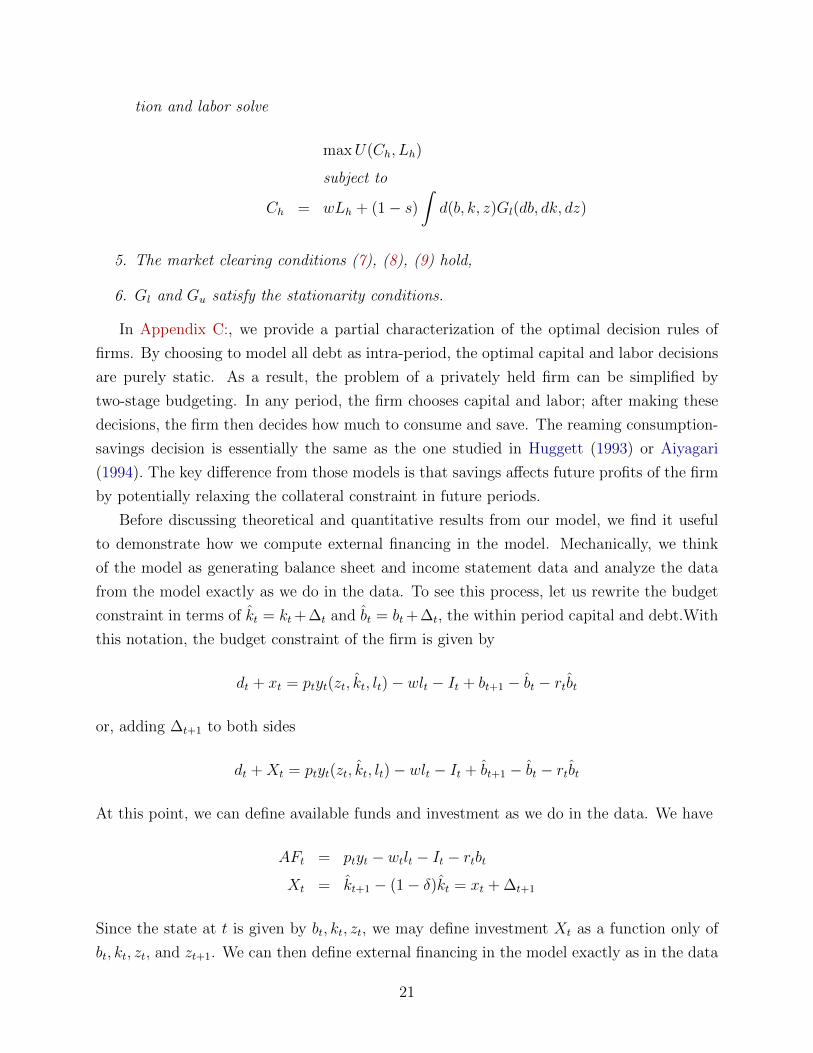
The left hand side of equation (1) represents the net financial flow into or out of the firm. If
the right hand side of equation (1) is positive so that the firm’s investment is less than the
cash generated by the firm in period t, then funds flow out of the firm. If the right hand
side of equation (1) is negative, then funds must flow into the firm as the firm’s investment
is greater than the cash it generated. Implicitly, by netting interest payments, rtbt, out of
available funds, but leaving dividend payments, stdt, on the left hand side, we assume that
dividends are not set in advance while interest payments cannot be re-negotiated.
Our aim, then, is to measure available funds defined as
AFt = πt + atet − rtbt
8
and physical investment, xt, as these measures are sufficient to determine whether a given
firm receives inflows of cash or makes cash outlays.
Our preferred statistic of how individual firms rely on external funds for investment is
given by
1
T
T∑t=1
∑i (Xit − AFit) 1[Xit≥AFit]∑
iXit
(2)
The statistic in equation (2) represents the average net financial inflow to firms whose in-
vestment is greater than their available funds as a fraction of total investment. The statistic
in equation (1) informs us about what fraction of aggregate investment must be financed
externally among a subset of firms, and, therefore, depends on well-functioning financial
markets.
2.2 Data Description
Our data sources for the U.S. include the Flow of Funds, the Statistics of Income, and
Compustat. Our data sources for the U.K. include the U.K. Economic Accounts, Compustat
Global, and Amadeus. We now describe each data set and how we measure available funds
and investment in each source.
2.2.1 U.S. Data
Aggregate Data. Aggregate U.S. data are from the Flow of Funds. Our measure of
aggregate available funds in the U.S. is the sum of Internal Funds (Table F.102 line 9) and
Dividends (Table F.201 line 3) of all non-farm nonfinancial corporate business. Note that we
add dividends here because the definition of Internal Funds has excluded them. Our measure
of aggregate investment is given by Capital Expenditures (Table F.102 line 11) of non-farm
nonfinancial corporate businesses.
Our second source of aggregate data is the Statistics of Income, specifically the Corpo-
ration Income Tax Returns, from 1991 to 2008. The Corporation Income Tax Returns data
set contains information on assets, liabilities, and income of all incorporated firms in the
U.S. classified by industry and by size of total assets. We focus on data classified by size of
total assets, specifically Table 2, which details the balance sheet and income statement of
active corporations. The advantage of using data from the Statistics of Income is that we
can analyze aggregate financial flows to firms of various sizes. In other words, we can analyze
whether the average small firm receives financial inflows even though in the aggregate all
firms make financial outflows. There are three limitations to working with data from the
Statistics of Income. The first is that the data cover all active corporations in the United
9
States, including agricultural and financial firms. The second limitation is that data are not
firm-level, so we can only analyze the net financial flows to an aggregated small firm. The
final limitation is that the size classes for the data are presented in nominal terms which can
introduce measurement bias (due to inflation and trend growth) as discussed in Gertler and
Gilchrist (1994).
In any year, an observation in this data set represents the aggregate over all firms with
assets within some nominal bounds. We measure available funds as total receipts less total
deductions plus deductions for depreciation, depletion, and amortization. To measure in-
vestment, we must construct a measure of the change in fixed assets from one year to the
next. Our measure of fixed assets in any year is the sum of depreciable assets, depletable as-
sets, intangible assets, and land less accumulated depreciation, depletion, and amortization.
To measure fixed asset growth among firms in any size class, we must make an educated
guess about how firms move across size classes from one year to the next. Our analysis
parallels that of Gertler and Gilchrist (1994). First, we re-aggregate the size categories into
two groups for “small” and “large.” Our cutoff for small firms is the threshold in assets
below which firms account for 30 percent of sales. The annual growth rate of assets for small
firms, then, is a weighted average of the growth rate of the cumulative asset classes on either
side of the thirtieth percentile at the start of the period. We then make adjustments to the
growth rate to correct for bias introduced by the fact that some firms may have shifted asset
classes. We also perform this procedure to construct a measure of the change in accumulated
depreciation, depletion, and amortization, which we then use as our measure of depreciation
over the year. Our measure of investment for small firms, then, is given by the growth in
fixed assets plus depreciation. Investment for large firms is constructed similarly.
Firm Level Data. Our primary source of firm-level data in the U.S. is Compustat.
Compustat provides financial data on firms actively traded on stock exchanges. We focus on
data from 1974 to 2010. We restrict attention to firms headquartered in the U.S. (location
code is USA) and we omit firms in Financial, Real Estate and Insurance industries (SIC
codes 60-67) and Government (SIC codes 91-99).
We construct available funds and investment for firms in Compustat as in the literature
on firm dependence on external financing (see Rajan and Zingales (1998)). In particular, we
measure available funds for a firm i in period t, as Operating Activities - Net Cash Flow (or
Funds from operations depending format of the statement of cash flows). Because our model
does not distinguish between physical investment in existing assets or acquisition of new
assets, we wish to include merger and acquisition activity as well as sales of property, plant
and equipment (as negative investment) in our measure of investment. We define investment
as the sum of capital expenditures and acquisition less sale of property plant and equipment.
10
Firms remain in our sample if we have sufficient data to construct our measures of
available funds and investment. We also require firms to have reported positive sales and
non-negative total liabilities. Our Compustat sample in the U.S. consists of about 51,000
firm-year observations, with roughly 1400 firm level observations in a typical year.
2.2.2 U.K. Data
Aggregate Data. Our source of aggregate data in the U.K. is the National Economic
Accounts. We measure available funds as the sum of gross disposable income and dividends of
non-financial corporations. Again, we add dividend payments back in because they have been
previously excluded in the construction of gross disposable income. We measure investment
as the sum of gross fixed capital formation, change in inventories, and acquisitions less
disposals of valuables and non-financial non-produced assets.
Firm Level Data. We have two sources of panel data on financial statements of firms
in the U.K. Our first data source is Compustat Global and only covers firms that are actively
traded on a stock exchange. We treat data from Compustat Global exactly as we do for
data from Compustat U.S.. Compustat U.K. sample consists of roughly 10,000 firm-year
observations between 1992 and 2009, with 550 firm level observations in a typical year.
Our primary source of firm level data for firms not actively traded on a stock exchange
is Amadeus. Amadeus contains financial information on over 18 millions private and public
companies in Europe with a focus on private companies. We restrict attention to the sample
of firms located in the United Kingdom from 2001 to 2009. We focus on data from the balance
sheet and profit and loss account. Data limitations prevent us from measuring available funds
and investment as we do in our Compustat sample, but we attempt to be as consistent as
the data allow us. Specifically, we measure available funds as the sum of profit (loss) for
period, which is roughly equivalent to income before extraordinary items, and depreciation.
We measure investment as the change in tangible assets plus depreciation.2 While we focus
on the privately held sample of firms in Amadeus, we also report statistics for the publicly
traded firms that are available to provide a comparison to the more comprehensive sample
of publicly traded firms from Compustat Global.3
2We have also measured investment by additionally including intangible assets, but this addition hadnegligible effects on our measure of external financing.
3We have also measured available funds and investment in this manner for both of our Compustatsamples. We found that this measure of investment is roughly consistent with our measure of investmentfrom Compustat, while this measure of available funds tends to understate the amount stated as OperatingActivities - Net Cash Flow. The primary discrepancy between these measures of available funds arises fromthe treatment of unclassified funds. To the extent that income before extraordinary items and depreciationlisted on the income statement of firms in Amadeus and Compustat are measured comparably, this findingsuggests that our measure of Available Funds in Amadeus may be biased downward, and thus our measure
11
Our sample of privately held firms consists of all non-government, non-financial firms
whose legal status is Private Limited Company or Public Limited Company and which are
not quoted on a stock exchange. We also restrict attention to firms that report non-negative
total liabilities (defined as the sum of current and non-current liabilities), non-negative total
assets, and non-negative sales. Because one component of our measure of investment is
the change in tangible assets, we must have at least two consecutive years of data for a
firm to remain in our sample. Our sample consists of over 980,000 firm-year observations
with roughly 100,000 firm-level observations in each year. Our Amadeus sample of Public
Limited Companies that are quoted on a stock exchange consists of roughly 3700 firm-year
observations with 400 firm-level observations in a typical year.
2.3 Facts about Financial Flows and External Financing
We now describe the facts on financial flows and external financing. We begin by describing
the lessons from aggregate or aggregated data, and then discuss the evidence on firm-level
dependence on external financing.
2.3.1 Aggregate Facts on Financial Flows
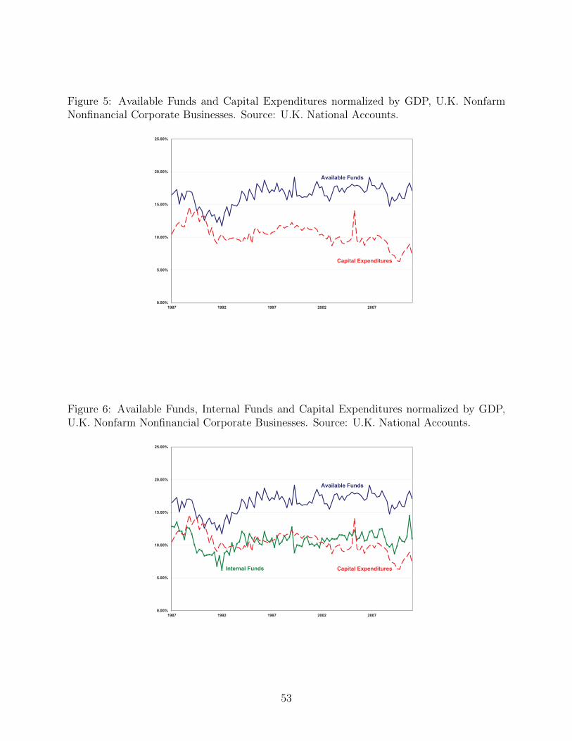
In figures 3 and 5 we plot available funds and investment for the U.S. and the U.K normalized
by nonfinancial corporate business GDP (in the U.S.) and by aggregate GDP (in the U.K.).
On average, available funds are roughly 1.25 times as large as investment in the U.S. and
1.6 times as large in the U.K. Moreover, in the U.S. available funds exceed investment by
roughly 3% on average over the entire sample. In this sense, the aggregate firm in the U.S.
and the U.K. does not rely on outside financing to fund investment.
We have argued that this observation presents a challenge for macroeconomics models
with a representative firm that faces a binding collateral constraint. There are two primary
responses to this challenge. First, to the extent that shareholders refuse to accept delayed
dividend payments, firms may not be able to self-finance their investment using available
funds net of dividends. In figures 4 and 6 we plot internal funds, or available funds net of
dividends, and investment in the U.S. and in the U.K. This data shows that internal funds are
on average roughly 95% of investment in the U.S. (though they are still 1.05 times as large as
investment in the U.K.). Representative agent models of financial frictions, then, must rely
on some mechanism to ensure that dividends in the aggregate do not respond to aggregate
shocks. In our model, because dividends of privately held firms are simply consumption of
of external financing in Amadeus may be biased upwards.
12
the undiversified owners of the firm, standard consumption smoothing motives will cause
dividends to not adjust to aggregate shocks.
The second response to the fact that available funds exceed investment in the aggregate
is that the aggregate statistics do not reveal information about how much individual firms
rely on external financing. The Statistics of Income data, by reporting data by asset size
classes, yields information on whether there different size classes of firms rely on external
financing. We find, however, that even small firms, in the aggregate, have sufficient available
funds to finance their investment. From 1992 to 2008, on average, available funds for large
firms are roughly 1.8 times as large as investment, and for small firms, available funds are
roughly 4 times as large as investment. We conclude that it is necessary to look at firm-level
evidence in order to gauge which firms rely on external financing and how much external
financing these firms need for investment.
2.3.2 Firm Level Evidence on External Financing
In this section, we provide evidence on the importance of external financing in firm level data.
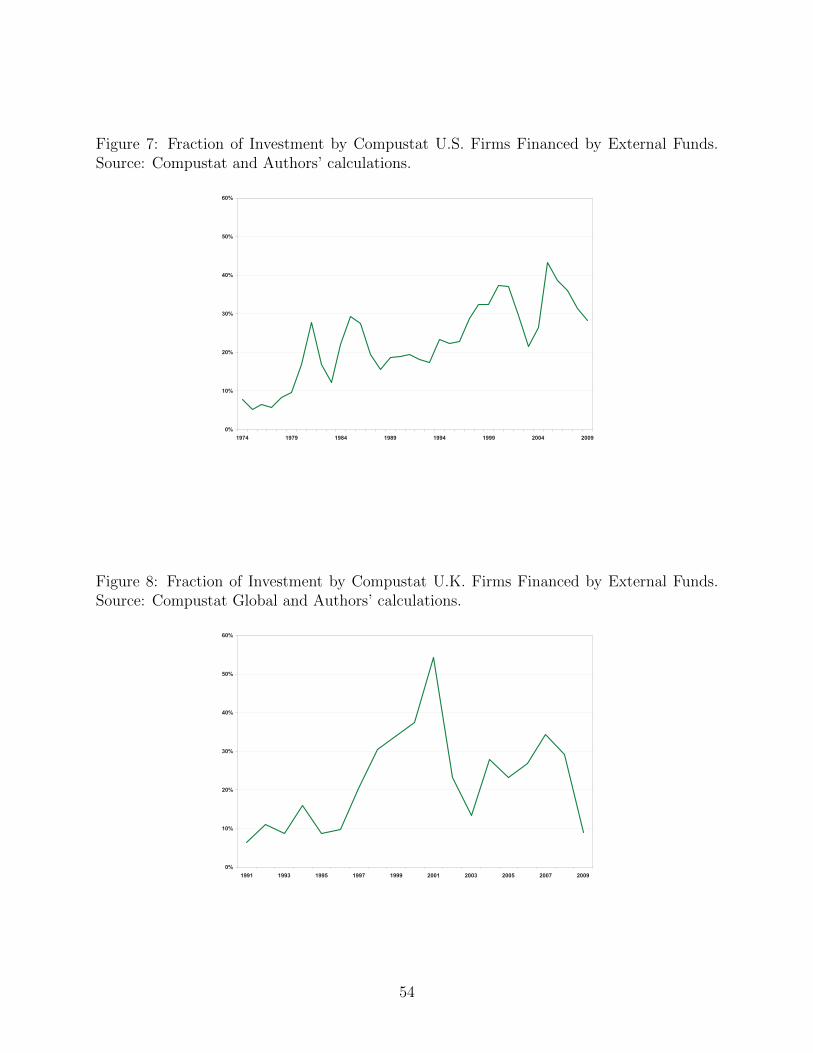
In Compustat in the U.S.. we find that on average roughly 23% of investment undertaken
by publicly held firms is financed externally. Similarly, in the U.K., we find that roughly
20% of investment by publicly held firms is financed externally.4
Analyzing U.K. data for privately held firms, we find that between 70% and 95% of
aggregate (Amadeus) investment is financed externally from 2001-2008. We provide a range
of estimates because our measure of external financing is sensitive to different treatments of
potential outliers. On the entire sample, we find that roughly 95% of investment is externally
finance. If we remove the three largest and smallest observations over the entire sample, then
we find that roughly 90% of investment is externally financed. When we winsorize the sample
at the 0.1% and 99.9% levels, removing observations in the smallest 0.1 percentile and largest
99.9 percentile of available funds and investment, we find that roughly 85% of investment
is externally financed; winsorizing at the 1 and 99 percentiles yields that on average 70% of
investment is externally financed.
It is possible that our splitting of data by privately and publicly held firms is merely
serving as a proxy for firm size. To address this issue, we construct a sample of privately
held and publicly traded firms of approximately the same size over the same horizon (2001-
2009). Specifically, we begin by following Gertler and Gilchrist (1994) to develop a sample
of “large” privately held firms. In any year, we classify a firm in our Amadeus sample as
“large” if its assets are over a threshold above which firms account for 70% of (Amadeus)
4This average excludes the year 1999 because of a lack of data availability for acquisitions. Alternatively,if we ignore acquisitions, then over the entire sample, roughly 8% of investment is externally financed.
13
sales. We then construct a sample of “small” publicly held firms in the U.K. similarly, except
we classify a firm as “small” if its assets are below the threshold in which firms account for
30% of (Compustat) sales.
Our sample of small publicly traded firms consists of roughly 6700 firm year observations
with firms holding on average £184 million in total assets (with a standard deviation of
£3.75 billion). Our sample of large privately held firms consists of roughly 18000 firms with
assets of roughly £840 million on average with a comparable standard deviation (roughly
£3.6 billion). Notice that our large, privately held firms are on average larger than our small,
publicly traded firms. Of course, the small publicly traded sample comprises the majority
of the data in our overall Compustat UK sample, while the large privately held sample
comprises roughly 2% of our Amadeus sample.
It is not surprising then that our sample of small publicly traded firms externally finance
roughly 21% of their investment. However, even after cleaning the large sample of the most
extreme values of investment and available funds, we find that large privately held firms
externally finance roughly 90% of their investment (small privately held firms externally
finance an even larger fraction of their investment – roughly 110%). Our conclusion is that
privately held firms externally finance a substantially larger fraction of their investment
than do publicly traded firms. As a result, we expect privately held firms to be much more
sensitive to exogenous changes in financing conditions than publicly held firms.
3 A Dynamic Model of Publicly Traded and Privately
Held Firms
In this section, we develop a dynamic model of publicly traded and privately held firms
and define a symmetric stationary equilibrium. In our model, all firms face constraints
in accumulating capital, have a monopoly in producing differentiated goods and require a
bundle of goods produced by other firms as an input to production. Publicly held firms are
owned by diversified households; privately held firms are owned by individual entrepreneurs.
3.1 Model and Equilibrium Definition
Environment. Time is discrete, lasts forever, and is indexed by t = 1, 2, . . .. Agents in the
model include households, final good producers, and intermediate good producers. There is
a single consumption good in the economy which is a composite good produced by a sector
of competitive final good producers. We normalize the price of the final good to be 1 in each
period. Final good producers aggregate the output of the intermediate good producers.
14
Each intermediate good producer has a monopoly in producing a differentiated output.
There are two classes of intermediate good producers: privately-held and publicly-held firms.
We normalize the total measure of intermediate good producing firms to be 1, and we assume
there is a fixed measure of privately held firms, s. A firm’s type is exogenously given and
fixed for the lifetime of the firm. Let firms i ∈ [0, s] denote the names of the s privately held
firms and i ∈ [s, 1] denote the names of the 1 − s publicly held firms in any period. Firms
exogenously exit at rate 1− ζ. Upon exit, firms are replaced by an otherwise identical firm
endowed with the exiting firm’s assets.
In our model, we distinguish between publicly and privately held firms by assuming that
publicly held firms are owned by and rebate dividends to diversified households. Privately
held firms are owned by individual entrepreneurs for whom the cost of delayed dividend
payments is forgone consumption.
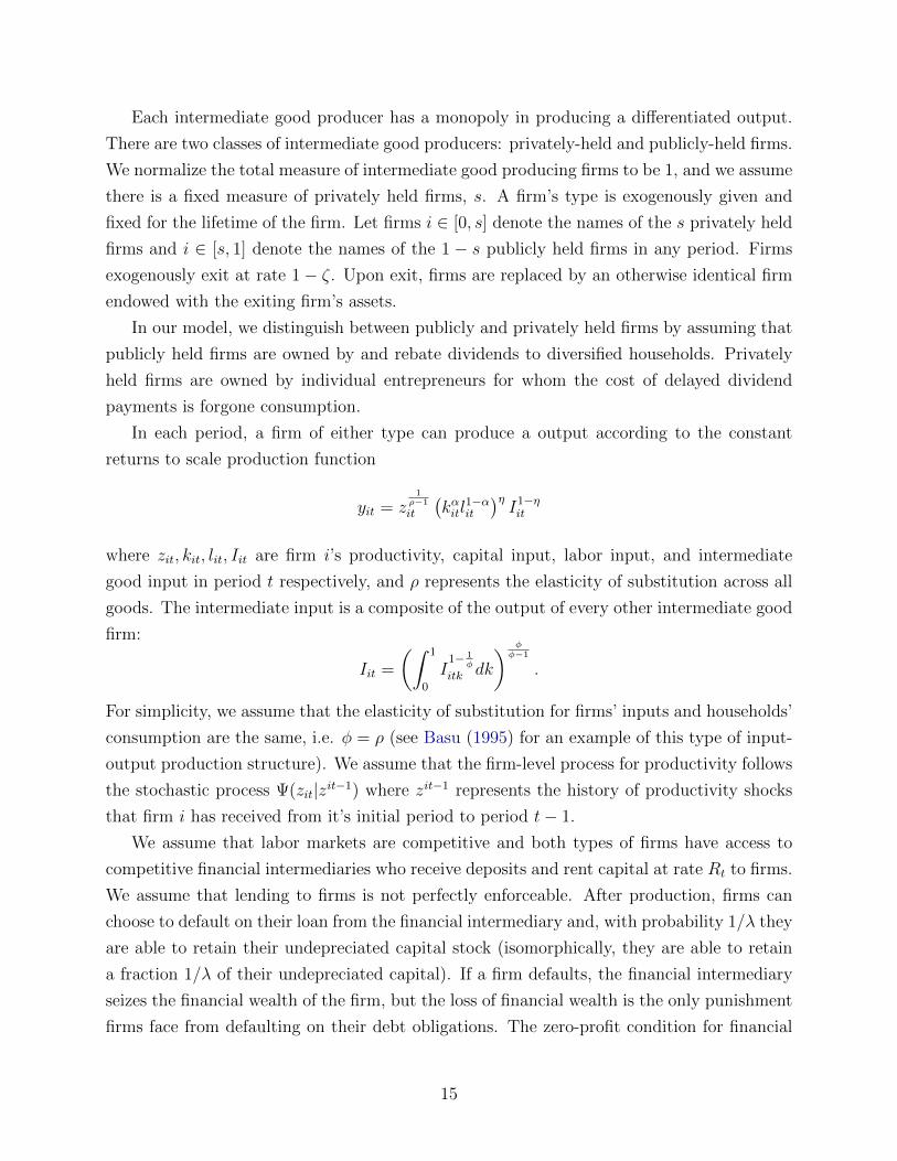
In each period, a firm of either type can produce a output according to the constant
returns to scale production function
yit = z1ρ−1
it
(kαitl
1−αit
)ηI1−ηit
where zit, kit, lit, Iit are firm i’s productivity, capital input, labor input, and intermediate
good input in period t respectively, and ρ represents the elasticity of substitution across all
goods. The intermediate input is a composite of the output of every other intermediate good
firm:
Iit =
(∫ 1
0
I1− 1
φ
itk dk
) φφ−1
.
For simplicity, we assume that the elasticity of substitution for firms’ inputs and households’
consumption are the same, i.e. φ = ρ (see Basu (1995) for an example of this type of input-
output production structure). We assume that the firm-level process for productivity follows
the stochastic process Ψ(zit|zit−1) where zit−1 represents the history of productivity shocks
that firm i has received from it’s initial period to period t− 1.
We assume that labor markets are competitive and both types of firms have access to
competitive financial intermediaries who receive deposits and rent capital at rate Rt to firms.
We assume that lending to firms is not perfectly enforceable. After production, firms can
choose to default on their loan from the financial intermediary and, with probability 1/λ they
are able to retain their undepreciated capital stock (isomorphically, they are able to retain
a fraction 1/λ of their undepreciated capital). If a firm defaults, the financial intermediary
seizes the financial wealth of the firm, but the loss of financial wealth is the only punishment
firms face from defaulting on their debt obligations. The zero-profit condition for financial
15
tkit , bit
zit realized Production
takes place
Buy/Sell Capital: it
kit+1 , bit+1
t+1
Figure 1: Timing of Production and Financing
intermediaries implies that the capital rental rate is given by rt + δ.
We now describe the problem and constraints of each type of agent in turn.
Final Good Producers. There are a large number of competitive final good producers.
Each of these producers can combine the output of the intermediate producers to produce a
composite final good according to the production function
Qt =
[∫i
q1− 1
ρ
it di
] ρρ−1
(3)
where qit is the input of firm i in period t, and ρ is the elasticity of substitution across all
goods in the economy. Perfect competition among final good producers ensures that we can
focus on a representative firm that solves
maxQ,qji
Q−∫i
pitqitdi
subject to the Q is given by the production function in (3) in each period. As before, the
final good producer’s problem gives rise to an inverse demand curve for each intermediate
good as a function of prices:
pi = Q1ρ
t q−1ρ
it .
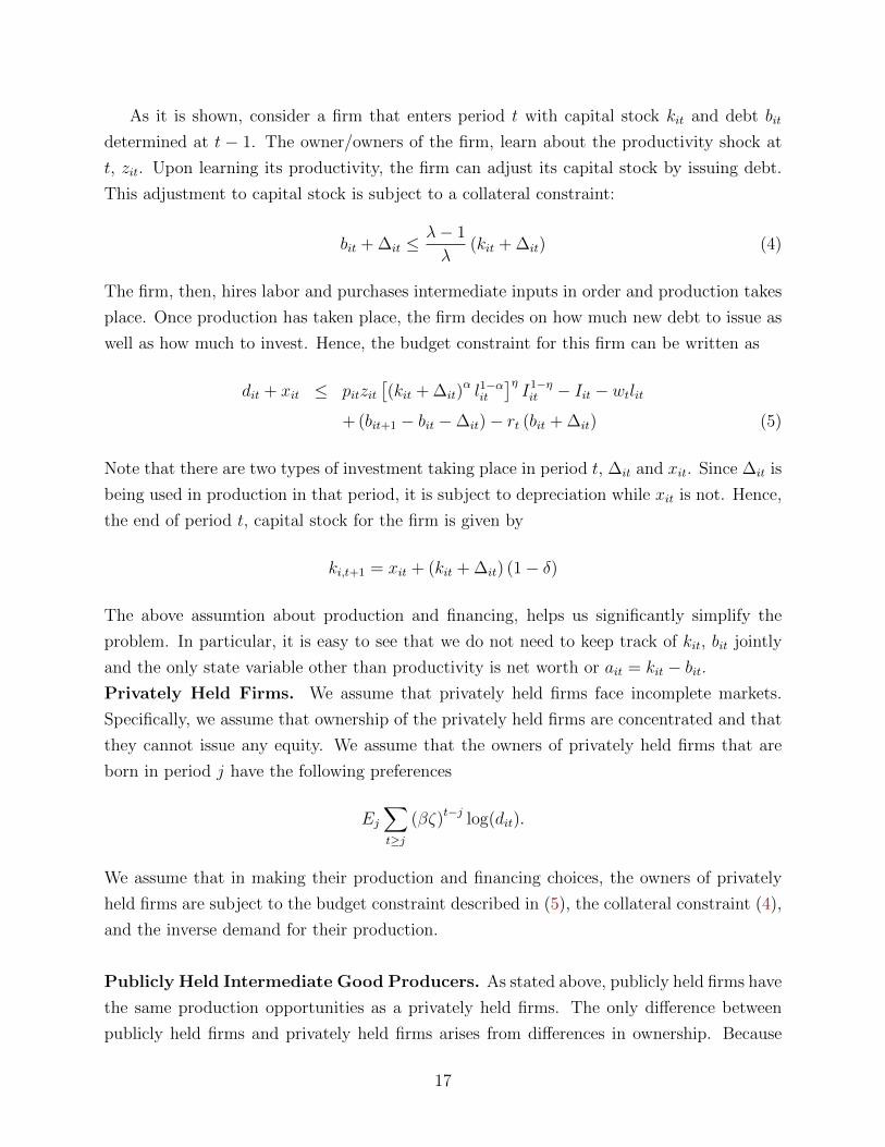
Finacing and Timing of Production. Here we describe the timing of production by
intermediate good firms and its interaction with firms’ financing decision. Throughout, we
assume that there is no equity financing. This assumption does not have any effect on
production decisions of publicly held firms. Figure 3.1, describe the timing of financing and
production decision of the intermediate good firms.
16
As it is shown, consider a firm that enters period t with capital stock kit and debt bit
determined at t − 1. The owner/owners of the firm, learn about the productivity shock at
t, zit. Upon learning its productivity, the firm can adjust its capital stock by issuing debt.
This adjustment to capital stock is subject to a collateral constraint:
bit + ∆it ≤λ− 1
λ(kit + ∆it) (4)
The firm, then, hires labor and purchases intermediate inputs in order and production takes
place. Once production has taken place, the firm decides on how much new debt to issue as
well as how much to invest. Hence, the budget constraint for this firm can be written as
dit + xit ≤ pitzit[(kit + ∆it)
α l1−αit
]ηI1−ηit − Iit − wtlit
+ (bit+1 − bit −∆it)− rt (bit + ∆it) (5)
Note that there are two types of investment taking place in period t, ∆it and xit. Since ∆it is
being used in production in that period, it is subject to depreciation while xit is not. Hence,
the end of period t, capital stock for the firm is given by
ki,t+1 = xit + (kit + ∆it) (1− δ)
The above assumtion about production and financing, helps us significantly simplify the
problem. In particular, it is easy to see that we do not need to keep track of kit, bit jointly
and the only state variable other than productivity is net worth or ait = kit − bit.Privately Held Firms. We assume that privately held firms face incomplete markets.
Specifically, we assume that ownership of the privately held firms are concentrated and that
they cannot issue any equity. We assume that the owners of privately held firms that are
born in period j have the following preferences
Ej∑t≥j
(βζ)t−j log(dit).
We assume that in making their production and financing choices, the owners of privately
held firms are subject to the budget constraint described in (5), the collateral constraint (4),
and the inverse demand for their production.
Publicly Held Intermediate Good Producers. As stated above, publicly held firms have
the same production opportunities as a privately held firms. The only difference between
publicly held firms and privately held firms arises from differences in ownership. Because
17
publicly held firms are owned by diversified households, they maximize the expected present
discounted value of their dividends under the stochastic discount factor of the households,
which, in the economy with no aggregate risk is simply βt. The objective of a publicly held
firm is given by the expected present discounted value of dividends, or
E0
∑t
βtdit.
Similar to privately held firms, the owners of the publicly held firms are subject to a budget
constraint, collateral constraint and inverse demand. Furthermore, we assume that they
cannot issue any equity, i.e., dit ≥ 0.
Bankruptcy and Entry. As it is clear above, public and private firms have different
discount factor. We interpret this as uninsurable bankruptcy by privately held firms. That
is we assume that every period, privately held firms becom bankrupt with probably 1 −ζ. Furthermore, in each period an equal measure of firms are borne and draw assets and
productivities from the joint stationary distribution of assets and productivities. That is we
assume that there are no losses in the value of the assets from bankruptcy. Later we perform
robustness on this assumption and assume that newly born firms assets are a fraction of th
amount of assets in the economy.
Households. In each period, households decide how much to work, how much to consume
and how much to save in the risk-free bond. They maximize lifetime expected utility
E0
∑t
βtU(Cht, Lht)
subject to the sequence of budget constraints
Cht + Aht+1 ≤ wtLht + (1 + rt)Aht +
∫ 1
s
citdi.
Equilibrium Definition. The aggregate state of the economy in any period can be summa-
rized by the distributions over debt, b, capital stock, a, and productivity, z, of privately held
firms which we denote by Gu(b, k, z), of publicly held firms which we denote by Gl(b, k, z) and
household assets Ah5. In a stationary equilibrium, we can summarize the market clearing
5Notice that given our assumptions about the timing of production and financing, net worth or k − b isa sufficient state variable and one need not keep track of both b and k. In other words, the distributionfunction Gu and Gl are only a function of k − b.
18
constraints using these distributions and the decisions made by privately held and publicly
held firms as functions of their individual states. We have four market clearing constraints.
In this section, we describe theoretical results that shed light on how the collateral con-
straints affect publicly held firms, the general equilibrium effects that arise in our model
due to differentiated goods and the input-output structure of productions, and how the re-
sponsiveness of the economy to collateral constraint shocks depends on how much external
financing occurs in the steady state equilibrium. Throughout this section, we denote net
worth by at = kt − bt and note that the set of constraints the firms are facing becomes
dt + at+1 = ptyt − wtlt − (rt + δ) kt + (1 + rt) at
kt ≤ λat
In this section, we use the above formulation for simplicty of exposition.
3.2.1 Equilibrium External Financing by Publicly Held Firms
In this section, we argue that because publicly held firms discount at the same rate as
household, in any equilibrium in which household consumption is stationary, publicly held
firms never face binding collateral constraints. To see this. consider the problem faced by
publicly held firms. If the non-negative dividend constraint or the collateral constraint ever
bind along any future history with positive probability, then the value of funds inside the
firm are worth more than the value of funds outside the firm. This result combined with
the fact that publicly held firms are risk neutral implies that in any such period, dividends
in that period must be zero. We state this result as the following lemma (the proof is in
Appendix C:).
Lemma 2. In any period t, if either the non-negative dividend constraint or the collateral
constraint in any history zs with s ≥ t then dividends in period t are zero.
The consequence of this lemma is that as long as either of a publicly held firm’s con-
straints bind, the firm’s asset level increases. To see this, note that stationarity of household
consumption implies that β(1+r) = 1 and thus 1+r > 1. The budget equation of a publicly
held firm with zero dividends implies
at+1 = Π(at, zt) + (1 + r)at > at
22
since profits are (weakly) positive and the interest rate is positive. Of course, as long as
zt ∈ [z, z] then there is a maximal optimal scale for the firm. Call this value k. Once the
publicly held firm’s assets satisfy at ≥ 1λk then the firm can simply save at in every future
period, rebate any profits and interest income to households in the form of dividends and
never face binding constraints again. Since the firm’s assets grow monotonically, they must
cross this threshold. As a result, in any stationary equilibrium, each publicly traded firm’s
assets must lie above 1λk.We then have the following proposition.
Proposition 3. In any stationary equilibrium, the collateral constraint never binds for any
publicly held firm.
An immediate consequence of the proposition is that there are a continuum of equilibria
indexed by asset holdings of publicly held firms above 1λk and a corresponding asset holding
of households so that capital markets clear at the given rental rate of capital, r = 1β− 1.
Since available funds for a given firm satisfy
AFt = ptyt − wtlt − rt(kt − at),
publicly traded firms in stationary equilibria always operate at optimal scale, we have AFt =
Π∗(zt)+rtat. Since there is an equilibrium for any a ≥ 1λk, available funds are indeterminate.
Consequently, the amount of external funds used by publicly held firms for investment is
indeterminate. We state this result as the following corollary.
Corollary 4. In any stationary equilibrium, the amount of external funds used by publicly
held firms to finance investment is indeterminate.
3.2.2 The Effects of Collateral Shocks on Unconstrained Firms
In any period in any stationary equilibrium of our model, some firms face binding collateral
constraints and others do not. Some of the firms that do not face binding constraints
are publicly held and others are privately held. One consequence of a shock that leads
to a tightening of the collateral constraint is that firms that do not face currently binding
collateral constraints become more productive relative to those firms for whom the collateral
constraint binds. As a result, these firms, absent any general equilibrium effects, would
increase their demand for production inputs and generate more output. This mechanism
dampens the effects of shocks to the collateral constraints.
We argue that general equilibrium effects cause shocks to the collateral constraints to
spill-over to these unconstrained firms and can dampen and even overturn their incentives to
increase production in response to a tightening of the constraints. In Appendix A:, we analyze
23
a static, partial equilibrium version of our model where households value consumption and
labor according to
U(C,L) = u
(C − ψ
1 + 1ε
L1+ 1ε
)as in Greenwood et al. (1988). We develop sufficient conditions for the equilibrium output
of every firm to be decreasing in the tightness of the collateral constraints. The key param-
eters that determine the strength of these general equilibrium spill-overs are the elasticity
of household labor supply,ε, the elasticity of substitution across goods, ρ, the labor share
parameter, α, and the intermediate input share parameter, η. We now state our main result
from Appendix A:.
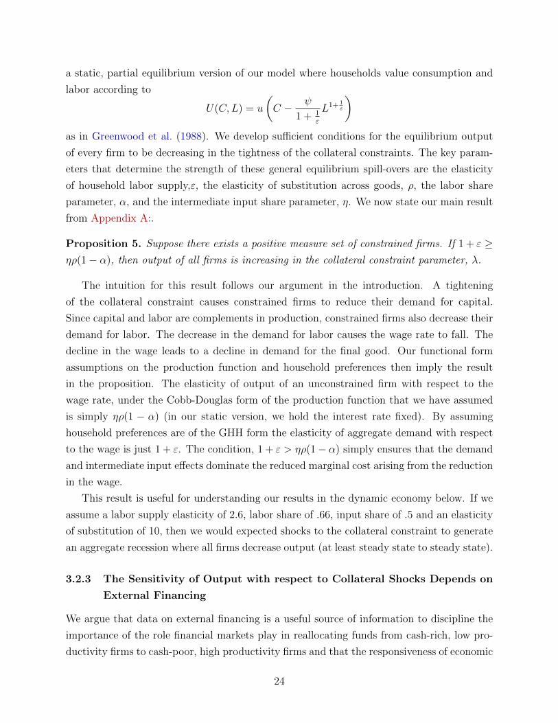
Proposition 5. Suppose there exists a positive measure set of constrained firms. If 1 + ε ≥ηρ(1− α), then output of all firms is increasing in the collateral constraint parameter, λ.
The intuition for this result follows our argument in the introduction. A tightening
of the collateral constraint causes constrained firms to reduce their demand for capital.
Since capital and labor are complements in production, constrained firms also decrease their
demand for labor. The decrease in the demand for labor causes the wage rate to fall. The
decline in the wage leads to a decline in demand for the final good. Our functional form
assumptions on the production function and household preferences then imply the result
in the proposition. The elasticity of output of an unconstrained firm with respect to the
wage rate, under the Cobb-Douglas form of the production function that we have assumed
is simply ηρ(1 − α) (in our static version, we hold the interest rate fixed). By assuming
household preferences are of the GHH form the elasticity of aggregate demand with respect
to the wage is just 1 + ε. The condition, 1 + ε > ηρ(1− α) simply ensures that the demand
and intermediate input effects dominate the reduced marginal cost arising from the reduction
in the wage.
This result is useful for understanding our results in the dynamic economy below. If we
assume a labor supply elasticity of 2.6, labor share of .66, input share of .5 and an elasticity
of substitution of 10, then we would expected shocks to the collateral constraint to generate
an aggregate recession where all firms decrease output (at least steady state to steady state).
3.2.3 The Sensitivity of Output with respect to Collateral Shocks Depends on
External Financing
We argue that data on external financing is a useful source of information to discipline the
importance of the role financial markets play in reallocating funds from cash-rich, low pro-
ductivity firms to cash-poor, high productivity firms and that the responsiveness of economic
24
output to financial market shocks depends on the importance of this role. In this section,
we use a stylized version of our dynamic model to illustrate this point theoretically.
In Appendix B:, we analyze a simplified version of our dynamic model in which there
are only privately held firms, goods are perfect substitutes, households do not save, and the
productivity process is i.i.d across firms and time. This version of our model corresponds
loosely to the theoretical models considered by Kiyotaki and Moore (2008) and, more specif-
ically, Kocherlakota (2009). Specifically, we assume that in every period, each firm has a
probability π of having productivity equal to 1 and probability 1 − π of having probability
equal to 0. By assuming that shocks are i.i.d. and goods are perfect substitutes, we are able
to construct closed form solutions for the equilibrium wage, output, and steady-state wealth
as well as compute external financing by hand.
We then consider the impact of changes in the tightness of the collateral constraint, λ, in
economies with different probability of being productive, π. One difficulty in this analysis is
that for economies with different productivity probabilities, π, a given change in λ represents
a different size “shock” to the economy. To account for this effect, for each π-economy, we
choose the collateral constraint parameter, λ(π) so that the aggregate debt-to-assets ratio in
the model is the same across all π-economies. Then, for each π-economy, we compare steady
state wealth and output in the λ(π) economy to that in the economy when λ = 1, in other
words, the autarkic version of that economy. Therefore, we are considering shocks to the
collateral constraint in each π economy that cause the aggregate debt-to-asset ratio to fall
from some constant to 0. We show that the difference in steady state wealth between the
λ(π), high debt economy, and the λ = 1, no debt economy is monotonically decreasing in the
probability of receiving a high productivity shock. At the same time, the amount of external
financing in the λ(π) high debt economy is monotonically decreasing in π. In this sense,
data on external financing is useful for disciplining the macroeconomic impact of shocks to
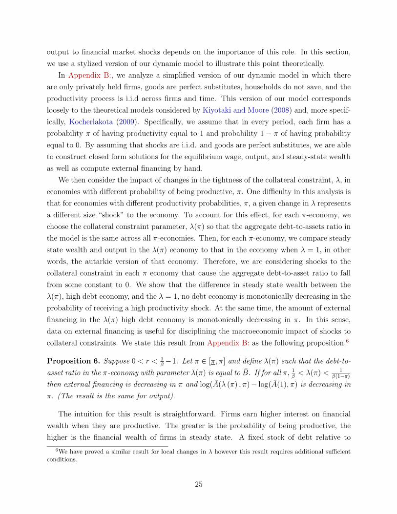
collateral constraints. We state this result from Appendix B: as the following proposition.6
Proposition 6. Suppose 0 < r < 1β−1. Let π ∈ [π, π] and define λ(π) such that the debt-to-
asset ratio in the π-economy with parameter λ(π) is equal to B. If for all π, 1β< λ(π) < 1
β(1−π)
then external financing is decreasing in π and log(A(λ (π) , π)− log(A(1), π) is decreasing in
π. (The result is the same for output).
The intuition for this result is straightforward. Firms earn higher interest on financial
wealth when they are productive. The greater is the probability of being productive, the
higher is the financial wealth of firms in steady state. A fixed stock of debt relative to
6We have proved a similar result for local changes in λ however this result requires additional sufficientconditions.
25
total assets generates a larger amount of wealth relative to autarky for an economy with
a lower probability of being productive since firms cannot accumulate as much financial
wealth. As a result, the difference between the autarky and the credit economy is largest
when the probability of being productive is the smallest. Of course, in economies where the
probability of being productive is low, when firms do become productive, they have typically
experienced a long spell of being unproductive. As a result, their assets have declined and
thus their available funds are low exactly when their investment exhibits a large increase.
As a result, economies with low probability of becoming productive exhibit a large degree of
external financing.
4 Calibration and Quantitative results
In this section, we calibrate the model and undertake exercises intended to illustrate the
contribution of changes in financial frictions to business cycle frequency fluctuations. We
calibrate the steady state of the model and then perform impulse response analysis. We
compare our results to those from a standard real business cycle model.
4.1 Calibration
Here we describe our calibration strategy. We have two sets of parameters: parameters that
are typically used in macroeconomic models, and parameters that we use our model to pin
down. As for the first set of parameters, we fix the discount rate to 0.96, targeting an annual
real interest rate of 4%. We set the annual depreciation rate, δ, to be 0.07 and we assume
that the exit rate of privately held firms, 1 − ζ, is 10%. This exit rate implies a ten year
survival rate of 34%, and is consistent with estimates from Dunne et al. (1988). Since ζ is a
major determinant of financial flows for privately held firms7, later, we perform robustness
checks on ζ. Furthermore, we set α, one of the parameters in the firm production function
to 0.3 and choose the elasticity of substitution across firms or goods to be ρ = 4 in line with
estimates from micro data evidence (see Burstein and Hellwig (2008)).
We parameterize household preferences as
U(c, l) = log
(c− ψ
1 + 1ε
l1+ 1ε
)We choose an elasticity of labor supply, ε, to be 2.6. We assume that there are no wealth
7When ζ is high, firms have stronger incentives to accumulate assets in order to overcome their collateralconstraint in the future. This could lower the amount of debt issued by privately held firms.This can dampenthe effect of a shock to λ on aggregate output.
26
effects on the labor-leisure tradeoff to highlight the role of the complementarity between
publicly held and privately held firms in our model, but note that choosing a more standard
form will reduce the sensitivity of output to changes in the severity of financial frictions
because declines in output by constrained firms will generate increases in output by uncon-
strained firms. Our choice of ε is in the range of macro estimates as documented by Chetty
et al. (2011), among others.
Next, we describe the set of parameters that are calibrated using our model. The key
parameters of the steady state calibration are the tightness of the collateral constraint and
the process for idiosyncratic firm level productivity. We calibrate λ, the tightness of the
collateral constraint to match average aggregate debt to total assets in the U.S. economy
since 1986, which is 0.49. We assume that firm level productivity follows an AR(1) process
so that
log zit = ρz log zit−1 + εit, εit ∼ N(0, σ2z).
We calibrate the standard deviation of the innovations to log productivity to match the vari-
ance in the firm-level debt-to-asset ratio in our Amadeus sample, which is 0.28. We calibrate
the persistence of the productivity process, ρz, so that in the model, 93% of investment by
privately held firms is externally financed (as in our benchmark Amadeus sample).
The measure of privately held firms, s, is chosen so that privately held firms account for
40% of corporate gross output. We compute this share by calculating the share of firms in
Compustat from gross output.8 Figure 4.1, plots this share from 1987 to 2009.
We choose the value of η (from the firm’s production function) so that input’s share of
gross output is .43 (Jones (2011)). Lastly, we choose ψ, which scales household’s disutility of
labor supply to generate aggregate hours of 0.3. The calibrated parameters are summarized
in table 4.1.
Before discussing the results of our quantitative exercise, it is useful to discuss how well
the model does in capturing some of the key moments in data. In particular, we are interested
in statistics relevant for privately held firms. In our calibration strategy, we have calibrated
the productivity process for firms to match external financing by private firm as well the
variance of debt to assets. One way to check the validity of our estimates is to compare
employment fluctuations in our model to data, as documented by Davis et al. (2007). In our
calibrated model, the cross-sectional dispersion in employment growth is 0.3 for privately
held firms while in data it is 0.4. We take this as a fairly close estimate and the amount
of idiosyncratic risk faced by our firms are not very far from that presented by Davis et al.
8We have calculated gross output by calculating the gross output at industry levels. This data is availablefrom BEA only from 1987. Moreover, this figure includes gross output by non-corporations as well. Thatmakes the share of privately held firms a bit biased upward.
27
Figure 2: Share of Private Firms in Gross Output
Parameter Explanation Value Targetβ Discount rate 0.96 Annual interest rate = 0.04ε labor supply elasticity 2.6 Frisch elasticityρ Elasticity of substitution 4 Burstein and Hellwig (2008)α Share of capital 0.3δ Depreciation rate 0.07ζ Survival rate 0.9 Dunne et al. (1988)
calibrated using the modelψ Coefficient on leisure 0.10 Aggregate hours = 0.3s Measure of private firms 0.42 Share of gross output by private
corporations=0.40η Share of Intermediated Inputs 0.43 Input share of gross output = 0.43
(Jones, 2011)λ Tightness of collateral constraint 3.50 Average debt to asset ratio = 0.49ρz Persistence of productivity shocks 0.70 Net financial inflow = 0.93σz Variance of productivity shocks 0.65 Variance of debt to asset
Table 1: Calibrated Parameter Values
(2007).
4.2 Shocks to λ
We now analyze the response of the economy to a purely unanticipated shock to λ. We
impose an initial shock to λ which then returns back to its steady state value. On impact,
28
agents in the economy immediately learn the entire path of λ. Our goal is to understand
how large a response in output is generated by a “typical” financial shock when agents place
zero probability on this event occurring.
We fix the decay of the impulse so that the (annual) half-life of the shock to λ is 1
year. We choose the size of the initial impulse so that on impact, the shock generates a
one standard deviation decline in aggregate debt-to-total assets in our model economy. In
the U.S., since 1986, the standard deviation of the aggregate debt-to-total assets ratio for
non-farm non-financial corporate businesses is 0.015 or roughly 3% (after using the HP-filter
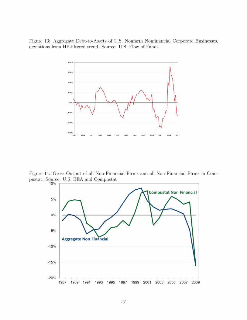
to filter out longer frequency movements). Figure (13) displays the residuals of the aggregate
debt-to-assets ratio at an annual frequency.
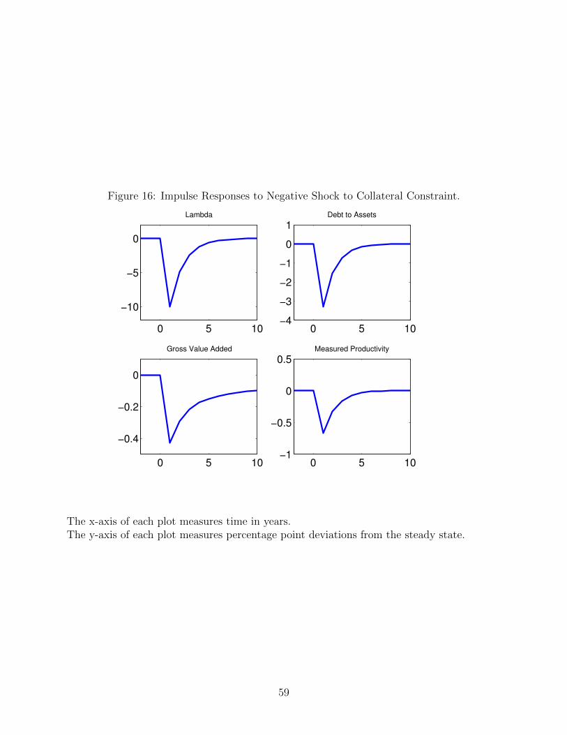
Figure 16 displays the path of deviations from steady state values of the collateral con-
straint parameter, λ, the aggregate debt-to-total asset ratio, and measured productivity.
We find that the impulse to the economy generates a roughly .45% decline in gross value
added on impact (we define gross value added as Gross Output less the aggregate use of
intermediate inputs). As we will discuss below, this is roughly 70% as large as the response
of output in our model to a “typical” productivity shock; ie: an aggregate productivity shock
that causes measured productivity to fall by one standard deviation of the measured solow
residuals in the U.S. economy. In this sense, we view the effect of the financial shock as
sizeable.
Given that the aggregate capital stock is fixed on impact, it is perhaps surprising that
output and labor fall on impact of the shock. This fall occurs because the tighter collateral
constraint leads constrained firms to reduce demand for capital and unconstrained firms to
increase their demand for capital (the rental rate of capital falls). The set of unconstrained
firms is typically made up of all publicly held firms and those privately held firms with low
productivity (relative to their assets). Thus, this reallocation of capital to unconstrained
firms implies more capital is installed by unproductive firms, leading to a decline in aggregate
productivity. This can be seen in the fourth panel of figure 16, which shows that measured
productivity on impact falls by 0.65%.
Second, we find that output does not recover by half until 2.5 years after the impulse
even though the shock has recovered by half after 1 year. In this sense, financial shocks have
persistent effects on output.
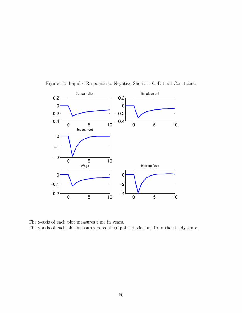
Third, we find that a financial shock causes consumption, employment, and investment to
move in the same direction of output. The paths for these objects, along with the paths for
wages and interest rates are depicted in Figure 17. The decline in employment is driven by the
reduction in the wage rate which, in turn, falls due to the decline in measured productivity.
The interest rate declines because the financial shock causes aggregate demand for capital
29
to fall. The decline in the wage and rental rate of capital, which is also the rate of return
households earn on their savings make final good consumers poorer and lead them to reduce
their consumption.
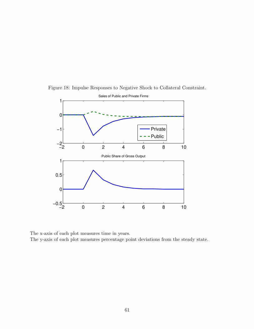
Fourth, Figure 18 displays the responses of sales by publicly and privately held firms as
well as the gross output share of the publicly held firms. We find that although sales of
privately held firms fall by roughly 1.5% on impact and remain below steady state for over
10 years, sales by publicly held firms actually rise by roughly .2% on impact of the shock.
By the second year after the impulse, sales of publicly held firms return to steady state, and
by the third year of the shock are below trend. The output share of publicly held firms,
however, remains above trend for the duration of the impulse.
The different response of sales by publicly and privately held firms initially is driven by
the increased use of capital by publicly held firms, none of which face binding collateral
constraints, and the fact that in response to the roughly 0.1% decline in the wage rate,
aggregate labor does not decline dramatically. Within two periods, however, as the supply
of capital falls, in response to the tightening of the collateral constraints, sales of both types
of firms are below the initial steady state. In this sense, our model is capable of generating
co-movement across the publicly held and privately held sectors, at least in the medium
term.
To comparing the response of these sectors in our model to data, in Figure 14 we plot
gross output of all non-financial firms in Compustat in the U.S. and gross output of all
non-financial firms in the U.S. (data from the BEA) as percentage deviations from a linear
trend. This figure shows that output of publicly held firms in compustat is highly correlated
with that of all non-financial firms, but not perfectly so.
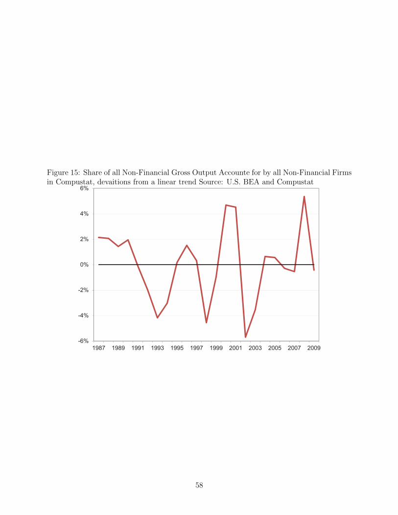
In terms of the share of output accounted for by publicly held firms in Compustat, which
we plot (again as deviations from trend) in figure 15, we observe that this share varies by
roughly 6% but not only around business cycle dates. For example, although the share
of output by Compustat firms is above trend from 2000 to 2001 and rises from 2007 to
2008, there are also significant movements (both increases and decreases) in the middle of
business cycle recoveries. Given these irregulat movements, we choose not use this evidence
to discipline our model.
The fact that output of publicly held firms falls below trend results only from the com-
plementarity in production across firms that we have discussed theoretically above. We have
performed sensitivity analysis with respect to the elasticity of substitution across goods, ρ,
the labor supply elasticitiy ε and the input-output structure governed by the parameter η.
However, in each of these cases, when we have re-calibrated our model to be consistent
with our target moments, we find that our benchmark result, that the response of aggregate
30
output to our calibrated financial shock is roughly 0.45% does not vary. What does change
is the composition of the response of privately versus publicly held firms. For example, with
a lower labor supply elasticitiy, a higher elasticity of substitution across goods, or no input-
output structure, we find that the gross output of publicly held firms does not fall below
trend at any point along the impulse response path. In this sense, we view trade linkages
as an important mechanism for generating co-movement of firms in response to a financial
shock.
Figure 19 displays the effect of the financial shock on the use of external funds measured
in the model as in our statistic in equation (2). Use of external funds declines on impact and
recovers back to its steady level. This result is driven primarily by the fact that most firms
that use external funds are constrained firms, and investment of constrained firms falls faster
than aggregate investment since most unconstrained firms actually increase investment in
response to lower wages and capital rental rates.
4.3 Shocks to Aggregate Productivity
We now compare the effects of financial shocks to the effects of aggregate productivity shocks
in our model. We perform a similar exercise as when we analyze financial shocks, only in this
section we consider the transition dynamics the result from a purely unanticipated decline
in aggregate productivity which slowly returns to steady state. Again, we fix the half-life of
the impulse to 1 year. In order to compare the magnitudes of the effects, we choose the size
of the shock so that measured productivity in the model falls on impact by one standard
deviation of the measured solow residual in the United States. This corresponds to roughly
a 1.% decline in measured productivity (at an annual rate).
We also compare the effects of productivity shocks in a version of our model without
collateral constraints. Specifically, we analyze our model economy in the case where there
are no privately held firms, but the process for idiosyncratic risk for publicly held firms is
the same as in our calibrated model above.
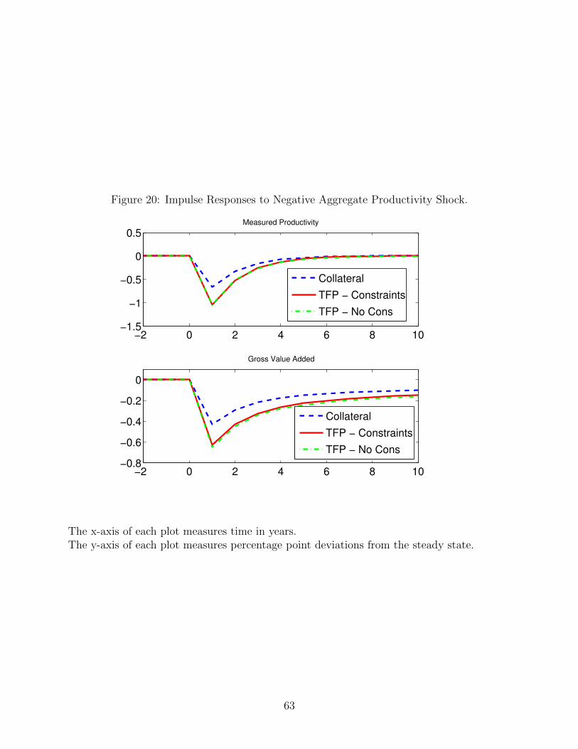
Figure 20 displays the impulse path for measured productivity following the shock to
aggregate productivity and gross value added (and, as in all of these pictures, the dashed
line represents the corresponding path from the response of our model economy to the cali-
brated financial shock). First, observe that a financial shock generates a decline in measured
productivity roughly 70% as large as this shock to measured productivity and that mea-
sured productivity recovers faster in response to an aggregate productivity shock than to a
financial shock.
Regarding gross value added, we find that a typical financial shock are roughly 70% as
31
large as the effects of a typical productivity shock. Note that in this model, the effects of
productivity shocks are dampened. In other words, a 1% decline in measured productivity
causes gross value added to fall by only roughly 0.7%. This is due primarily to the monopoly
distortions, which become less severe in response to a decline in aggregate productivity. Also
note that the model with and without collateral constraints generate roughly the same effect
on output. This is a well known result going back at least to Kocherlakota (2000).
Finally, figure 21 depicts the response of aggregate debt-to-total assets ratio as well as
the use of external funds in the model (with collateral constraints). Notice that debt-to-
assets do not move at all and the use of external funds as defined in equation (2) rises in
response to the shock. Demand for debt by firms falls as the level of capital they optimally
want to install is lower in response to the aggregate productivity shock, but their demand
for capital has also fallen by roughly an equivalent amount, causing the debt-to-asset ratio
to remain roughly stable. The response of the use of external funds, on the other hand, is
in the opposite direction of the response following a financial shock. The reason for this is
that when aggregate productivity declines, the collateral constraints for constrained firms
are relaxed as the unconstrained level of investment they want to undertake is lower. As a
result, investment by constrained firms falls by less than the aggregate, leading the use of
external funds to rise.
In this sense, although productivity shocks and financial shocks have similar size effects
on output, they affect financial flows in very different ways. It is not surprising that time
series variation in aggregated financial flows statistics may be useful in distinguishing be-
tween productivity and financial shocks. Given longer time series data on financial flows for
privately held firms, these differences could be useful in undertaking just such an analysis.
4.4 Sensititivy with Respect to Exit Risk
We conclude our quantitative section with a brief discussion of the sensitivity of our results
to the magnitude of the exit risk in our model, which is governed by the parameter ζ. First,
consider an increase in the survivial rate, holding the remaining parameters of the model
fixed. IN this example, we increase ζ from 0.9 to 0.95.
The steady state of this economy differs significantly along the key financial flows mo-
ments that we target from that of our benchmark economy. In particular, in this economy,
the aggregate debt-to-assets ratio is 0.30% (instead of 0.49) and the use of external funds
is 1.63 (instead of .93). The main difference between these economies is that the average
wealth of owners of privately held firms is higher. In fact, the book value of the net worth
of owners of privately held firms is 60% of aggregate capital; in our benchmark, this value is
32
20% of aggregate capital.
Somewhat surprisingly, the use of external funds in this model is significantly higher than
in our benchmark economy. The difference is that in this version of the model, most use
of external funds comes in the form of changes in negative debt holdings; in other words,
firms in this economy use external funds when they draw down against their net worth. One
way to see this difference is to note that in this economy, rougly 20% of privately held firms
face binding collateral constraints in any period (as opposed to 40% in our benchmark), but
26% of firms use external funds for investment (as opposed to 17%). In addition, over 35%
of owners of privately held firms have a negative debt position. These results combine to
ensure that the aggregate debt-to-assets ratio is too low relative to our benchmark economy.
The consequence of this difference is that if we impose the same impulse response as in
our benchmark model, aggregate output falls by only 0.2%. We view this kind of sensitivity
of our result that financial shocks have sizeable effects as arising for the wrong reasons. That
is, the effects are small only because these firms do not use as much debt as they do in the
data.
5 Conclusion
We have analyzed the effect of disturbances to financial markets in a quantitative model
where financial frictions operate through collateral constraints. We used data on firm-level
financial flows to discipline the importance of financial markets in the model and found that
the decline in macroeconomic output generated by a calibrated tightening in the collateral
constraint is roughly consistent with that generated by a calibrated decline in aggregate
productivity in a standard real business cycle model.
These results suggest that shocks to collateral constraints may contribute to a significant
fraction of business cycle volatility. A quantitative version of our model with aggregate
shocks to collateral constraints and productivity is in progress.
An important question for future analysis is the extent to which our quantitative results
are sensitive to our decision to model collateral constraints as working capital constraints
as opposed to constraints on new investment. We also intend to study this question by
analyzing a similar version of our model where capital is not fully mobile and the financial
frictions manifest as constraints on new investment.
33
Appendix A: Static Version of our Model
In this Appendix, we develop a static version of our model in order to establish the main
economic mechanism of the model. We use the static model to illustrate how shocks to the
collateral constraint affects both firms for whom the constraint binds and also those for whom
the constraint does not bind. We derive a sufficient condition on the model parameters under
which a tightening of the collateral constraint leads all firms to reduce output in equilibrium.
Consider a static economy populated by a continuum of intermediate good firms, a rep-
resentative final good producer, and a representative household.
Intermediate Good Producers. Each intermediate good firm i ∈ [0, 1] has an asset
level ai and productivity zi. Moreover, (ai, zi) is distributed according to F (a, z). An
intermediate good firm with productivity zi and assets ai, rents labor, l, and capital, k, rents
out its assets ai and purchases an amount of the final good, I, to be used as an input to
production according to the production function
qi = z1ρ−1
i
(kαl1−α
)ηI1−η
Each firm may rent capital up to a multiple of the value of the firm’s assets. Specifically, we
impose a collateral constraint so that the amount of capital rented by a firm with asset level
ai is bounded by λai where λ ≥ 1. One can rationalize this type of constraint by a model of
moral hazard or limited enforcement. In line with the rest of the literature, we impose this
constraint and do not provide a formal micro foundation for it.
Final Good Producer. The final good producer uses a bundle of inputs purchased
from intermediate good firms and takes their prices as given. Given a bundle {qi}i∈[0,1], the
final good producer uses the following Dixit-Stiglitz production function:
Q =
[∫ 1
0
qρ−1ρ
i dF (i)
] ρρ−1
with ρ > 1.
Households. We assume that there is a representative households who buys the final
good and provides labor to intermediate good producers. Following Greenwood et al. (1988),
we assume that household preferences are given by
U
(c− ψ l1+ 1
ε
1 + 1ε
)
Markets. We assume that the labor market is competitive at wage level w. As for capital
34
market, we assume that the economy is small and open. That is, there exist suppliers of
capital that have deep pockets and inelastically supply capital at a given interest rate r.
This is an assumption that simplifies the analysis; under this assumption, when we perform
comparative statics, we do not need to consider general equilibrium effects that arise from
changes in the interest rate for capital. Similar analysis can be done in a closed economy.
Moreover, we assume that there is monopolistic competition across intermediate good
firms and prices are given by pi. The final good producer takes these prices as given and
intermediate good producers take the demand function for intermediate output as given. We
normalize the price of final good to 1.
Given the above market structure, the final good producer’s maximization problem is
given by
maxqi
[∫ 1
0
qρ−1ρ
i dF (i)
] ρρ−1
−∫ 1
0
piqidF (i) .
The resulting demand for intermediate good i is given by
q− 1ρ
i Q1ρ = pi.
Given this demand function, each intermediate good firm maximizes its profit subject to its
collateral constraint:
πi = maxk,l,I,pi
piz1ρ−1
i
(kαl1−α
)ηI1−η − wl − rk − I + rai (16)
subject to
pi = Q1ρ
(z
1ρ−1
i
(kαl1−α
)ηI1−η
)− 1ρ
k ≤ λai
We say that a firm is financially constrained if the collateral constraint is binding for a firm
in equilibrium and is financially unconstrained otherwise.
To complete the definition of competitive equilibrium, we need to specify the household’s
optimization problem as well as market clearing conditions. The representative household’s
optimization problem is given by
maxc,L
U
(c− ψ L
1+ 1ε
1 + 1ε
)
35
subject to
c ≤ wL+
∫ 1
0
πidF (i) .
Labor market and product market clearing are given by∫ 1
0
lidF (i) = L
c+
∫i
IidF (i) = Q.
Hence a competitive equilibrium of this economy is given by{{ki, li, Ii, pi}i∈[0,1] , c, L,Q,w
}that satisfies the above conditions.
Because of monopolistic competition, the revenue function of the firm exhibits decreasing
returns to scale. As a result, for every z, there is an unconstrained optimal scale, which is
increasing in z. Not surprisingly, then, every z, there is a threshold in assets, say a∗(z) such
that firms with assets and productivity (a, z) with a ≥ a∗(z) are financially unconstrained
and if a < a∗(z) the firm is financially constrained. We state this result along with optimal
capital, labor, and intermediate input decisions for firms in the following lemma (the proof
is omitted).
Lemma 7. For every z, there exists a∗(z) such that for a ≥ a∗(z), k(a, z) ≤ λa and for
a < a∗(z), k = λa. Furthermore, a∗(z) satisfies
a∗(z) =1
λ[ν(1− η)]
(1−η)ν1−ν
(αηνr
)1+ αην1−ν(ν(1− α)η
w
) (1−α)ην1−ν
Qz.
If a ≥ a∗(z) then
k(a, z) = [ν(1− η)](1−η)ν1−ν
(αηνr
)1+ αην1−ν(ν(1− α)η
w
) (1−α)ην1−ν
Qz
if a < a∗(z) then k(a, z) = λa. Finally,
l =
(ν(1− α)η
w
) 1−(1−η)ν1−(1−αη)ν
(ν(1− η))(1−η)ν
1−(1−αη)ν (Qz)(1−ν)
1−(1−αη)ν kαην
1−(1−αη)ν
I =[ν(1− η)(Qz)1−ν (kαl1−α)ην] 1
1−(1−η)ν
where ν = 1− 1ρ.
Given the decisions of firms along with optimal labor supply of households, we can
36
characterize equilibrium output, Q and the wage rate, w using the production function of
the final good producer and the labor market clearing conditions. Given these equilibrium
values, we can show that the equilibrium wage rate is decreasing in the collateral constraint
parameter λ. This final result follows because a relaxing of the constraint must increase
aggregate capital demand and therefore labor demand causing the wage to rise. We have
the following lemma.
Lemma 8. Any competitive equilibrium must satisfy the following:
1. Q = 1
(1−α)η(1− 1ρ)ψ−εw1+ε,
2. The equilibrium wage, w, is decreasing in λ.
Proof. Given capital, labor and intermediate input demand, we can construct aggregate
excess output and labor as functions of prices r, w, and output Q. Specifically, let A∗ =
{(a, z) : a ≥ a∗(z)}
Qν =
∫qνG(da, dz) (17)
=
(ν(1− α)η
w
) νη(1−α)1−ν
(ν(1− η))ν(1−η)1−ν
(αηνr
) αην1−ν
Qν
∫(a,z)∈A∗
zG(da, dz)
+
(ν(1− α)η
w
) νη(1−α)1−(1−αη)ν
(ν(1− η))ν(1−η)
1−(1−αη)ν Qν(1−ν)(1−αη)1−(1−αη)ν λ
αην1−(1−αη)ν
∫(a,z)/∈A∗
z(1−ν)
1−(1−αη)ν aαην
1−(1−αη)νG(da, dz)
Labor Demand is just a function of output. We have
l =
((1− α)ην
w
)Q1−νqν .
Thus ∫lG(da, dz) =
((1− α)ην
w
)Q1−ν
∫qνG(da, dz)
Household labor supply given our assumed form for household preferences (GHH) is just
ψ−εwε.Thus labor market clearing is simply
ψ−εwε =
((1− α)ην
w
)Q
and, therefore, aggregate output in equilibrium satisfies
Q = ψ−ε((1− α)ην)−1w1+ε.
37
Re-write Q from (17) as
1 =
(ν(1− α)η
w
) νη(1−α)1−ν
(ν(1− η))ν(1−η)1−ν
(αηνr
) αην1−ν∫
(a,z)∈A∗zG(da, dz) (18)
+
(ν(1− α)η
w
) νη(1−α)1−(1−αη)ν
(ν(1− η))ν(1−η)
1−(1−αη)ν Q−αην
1−(1−αη)ν λαην
1−(1−αη)ν
∫(a,z)/∈A∗
z(1−ν)
1−(1−αη)ν aαην
1−(1−αη)νG(da, dz)
Analyzing the derivative with respect to λ,we have
0 =
(ν(1− α)η
w
) νη(1−α)1−ν
(ν(1− η))ν(1−η)1−ν
(αηνr
) αην1−ν∫
(a,z)∈A∗zG(da, dz)
×[−νη(1− α)
1− ν1
w
dw
dλ
]+
(ν(1− α)η
w
) νη(1−α)1−(1−αη)ν
(ν(1− η))ν(1−η)
1−(1−αη)ν Q−αην
1−(1−αη)ν λαην
1−(1−αη)ν
∫(a,z)/∈A∗
z(1−ν)
1−(1−αη)ν aαην
1−(1−αη)νG(da, dz)
×[− νη(1− α)
1− (1− αη)ν
1
w
dw
dλ− αην
1− (1− αη)ν
1
Q
dQ
dλ+
αην
1− (1− αη)ν
1
λ
]Suppose dw
dλ≤ 0. Then dQ
dλ≤ 0. Then we must have
− νη(1− α)
1− (1− αη)ν
1
w
dw
dλ− αην
1− (1− αη)ν
1
Q
dQ
dλ+
αην
1− (1− αη)ν
1
λ≤ 0
and sinceαην
1− (1− αη)ν
1
λ> 0
we haveνη(1− α)
1− (1− αη)ν
1
w
dw
dλ+
αην
1− (1− αη)ν
1
Q
dQ
dλ> 0
but the coefficients are all positive so this is a contradiction. As a result, the wage must be
increasing in λ.
We are now ready to state our necessary and sufficient condition for a tightening of the
collateral constraint to cause both financially constrained and financially unconstrained firms
to decrease output. Using the optimal production decisions of firms, we can show that a
38
financially unconstrained firm’s output satisfies
qi =
(ν(1− α)η
w
) η(1−α)1−ν
(ν(1− η))1−η1−ν
(αηνr
) αη1−ν
Qz1ν
= κw−η(1−α)1−ν Q
A one percent increase in w causes Q to increase by 1 + ε percent and w−η(1−α)1−ν to decrease
by η(1−α)1−ν . Hence, output of financially unconstrained firms is increasing in w or λ if and
only if 1 + ε ≥ ηρ(1− α). We then have the following proposition.
Proposition 9. Suppose there exists a positive measure set of constrained firms. If 1 + ε ≥ηρ(1− α), then output of all firms is increasing in the collateral constraint parameter, λ.
39
Appendix B: External Financing in a Simplified Ver-
sion of our Dynamic Model
In this section, we analyze a version of our model with perfect competition, perfect substi-
tutes, and an i.i.d. process for firm level productivity. Specifically, we assume that in every
period, each firm has a probability π of having productivity equal to 1 and probability 1−πof having probability equal to 0. We solve analytically for the equilibrium and the amount
of external financing used by firms in the model. We then compare the effect of changes in
the collateral constraint parameter, λ, across economies with different probabilities of high
productivity, π.
In particular, for each π-economy, we choose the collateral constraint parameter, λ(π)
so that the aggregate debt-to-assets ratio in the model is the same across all π-economies.
We show that even though the debt-to-asset ratio is held constant, the amount of external
financing is decreasing the probability of receiving a high productivity shock. Then, for each
π-economy, we compare steady state wealth in the λ(π) economy to that in the economy
when λ = 1, in other words, the autarkic version of that economy. We show that the
difference in steady state wealth between the λ(π), high debt economy, and the λ = 1, no
debt economy monotonically decreasing in the probability of receiving a high productivity
shock.
Model and Solution
In this simplified version of our model, firms are identical, produce a homogeneous final
output good, and the process for firm level productivity is given by
zt =
{1 w.prob π
0 w.prob 1− π
where the shocks are independent and identically drawn across firms and time. We assume
a small open economy with a fixed interest rate that satisfies 0 ≤ r ≤ 1β− 1.
The problem of a firm in any period can be written recursively as
V (a, z) = max ln(c) + βEV (a′, z′)
subject to
c+ a′ ≤ (1 + r)a+ maxk≤λa,l
zkαl1−α − wl − (r + δ)k
40
Clearly a firm with z = 0 chooses k = 0, l = 0. It is straightforward to show that profits for
a firm with z = 1 are given by[α
(1− αw
) 1−αα
− (r + δ)
]λa.
Using this result, we may write the recursive problem of the firm as
V (a, z) = max ln(c) + βEV (a′, z′)
s.t.
c+ a′ ≤
{zλ
[α
(1− αw
) 1−αα
− (r + δ)
]+ (1 + r)
}a.
Given our assumed form of preferences along with i.i.d. shock process for productivity, we
immediately have that the savings functions are linear in asset holdings and given by
a′(a, 1) = β
{λ
[α
(1− αw
) 1−αα
− (r + δ)
]+ (1 + r)
}a (19)
a′(a, 0) = β(1 + r)a.
The law of motion for assets in a steady state equilibrium yields the equilibrium wage rate
which must satisfy
1 = β(1 + r) + βπλ
[α
(1− αw
) 1−αα
− (r + δ)
].
Labor market clearing (with aggregate labor normalized to 1), then, defines steady state
wealth:
A(λ, π) =
[αβ(πλ)α
1− β(1 + r) + β(r + δ)πλ
] 11−α
.
We now turn to analyzing the amount of external financing firms rely on as well as the
amount of aggregate debt and assets.
External Financing
First, as in our quantitative model, we define available funds and investment by re-writing
the budget
ct + at+1 = ztkαt l
1−αt − wlt − (r + δ)kt + (1 + r)at
41
of a firm with an explicit definition of debt bt = kt − at. We then have
ct + kt+1 − (1− δ)kt = zαt kαt l
1−αt − wlt − rbt + bt+1 − bt.
We then define available funds, debt, and investment as
AFt = kαt l1−αt − wlt − rbt
bt = kt − atXt = kt+1 − (1− δ)kt
Available funds for specific firms depends on their asset holdings and their productivity in
any period. All of the derivations are included below. Available funds for firms with assets
at and productivity zt satisfy
AFt(at, zt) =
{at
[1−β(1+r)
βπ+ λδ + r
]if zt = z
atr if zt = 0
Investment, of course, depends on productivity and assets in period t+ 1 since these factors
determine the amount of capital a firm uses in period t+ 1. Since assets in period t+ 1 are
functions of assets and productivity in period t we may define investment as functions only
of at, zt and zt+1. We have
Xt(at, zt, zt+1) =
atλ[δ + 1−π
π(1− β(1 + r))
]if zt = z, zt+1 = z
−at(1− δ)λ if zt = z, zt+1 = 0
atλβ(1 + r) if zt = 0, zt+1 = z
0 if zt = 0, zt+1 = 0
.
To aid us in defining external financing, it is useful to define the amount of excess available
funds a firm has for investment. Define AF −X for each firm:
AF −X =
at
[r + (1− β(1 + r))
[1−βλ(1−π)
βπ
]]if zt = z, zt+1 = z
at
[1−β(1+r)
βπ+ λ+ r
]if zt = z, zt+1 = 0
at [r(1− λβ)− λβ] if zt = 0, zt+1 = z
atr if zt = 0, zt+1 = 0
We use this expression to get a sense of which firms are likely to rely on external financing.
Clearly unproductive firms in period t+ 1 will not typically rely on outside funds since both
firms have 0 or negative investment. Typically, the firm that switches from unproductive in
42
period t to productive in period t+ 1 (zt = 0, zt+1 = z) will rely on outside funds since that
firm has low available funds in period t but a high amount of investment (when λ is sufficiently
large). Finally the firm that is productive in two consecutive periods (zt = z, zt+1 = z) will
typically not rely on external funds since that firm’s available funds are large in period t,
however this is sensitive to the choice of λ since, as λ becomes large, even though the firm
has high available funds, the amount the firm invests grows as well.
Before turning to the effects of changes in λ, we point out that in the aggregate, inde-
pendent of the collateral constraint and the probability of being productive, in the aggregate
firms can self finance all of their investment. To see this, notice that in the aggregate,
investment is simply
δπλA
as productive firms are maintaining the capital stock, and available funds are given by
A
[r +
1− β(1 + r)
β+ πλδ
]Thus, in the aggregate, firms can self-finance all of their investment as the aggregate excess
is given by
A
[r +
1− β(1 + r)
β
]Finally, we have the aggregate debt-to-asset ratio:
π(λ− 1)
πλ+ 1− π. (20)
To see this final result, note that debt is just k − a for firms with k ≥ a. The only firms
with k ≥ a are those with z = 1. Hence, aggregate debt is simply πA(λ − 1). Total assets,
however, is not simply wealth, or A. Total assets are capital installed by firms with z = 1
and assets of firms with z = 0 since these firms, in effect, have claims to financial assets.
Hence, total assets are given by πλA+ (1−π)A. Note that the aggregate debt-to-asset ratio
for any π varies from 0 to 1 as λ varies from 1 to ∞.
Relating External Financing to the Importance of Financial Markets
Consider the following exercise. For any π, choose λ so that the debt-to-asset ratio is
constant (same amount of aggregate debt relative to assets in every π economy). Then,
consider the difference in steady state wealth when λ = λ(π) and when λ = 1 (or when debt-
to-assets falls from the constant level to 0). I do this because the metric is easier to analyze
43
(with respect to π) than is the derivative of steady state wealth. We have the following
proposition.
Proposition 10. Suppose 0 < r < 1β−1. Let π ∈ [π, π] and define λ(π) such that the debt-to-
asset ratio in the π-economy with parameter λ(π) is equal to B. If for all π, 1β< λ(π) < 1
β(1−π)
then external financing is decreasing in π and log(A(λ (π) , π)− log(A(1), π) is decreasing in
π. (The result is the same for output).
Proof. The assumptions of the proposition ensure that the only firm relying on external
funds for investment is the firm switching from unproductive to productive. Formally, these
assumptions place bounds on π for a given B. To see this, using the definition of debt-to-
assets in equation (20), we have that
λ(π) =B
π(1− B)+ 1. (21)
Since λ(π) is decreasing in π, we can replace the assumption on λ(π) by ensuring that
1
β≤ B
π(1− B)+ 1
andB
π(1− B)+ 1 ≤ 1
β(1− π)
It can be shown that these conditions are consistent with π > π.
Recall the definitions of external financing for the (zt = 0, zt+1 = z) and the (zt =
z, zt+1 = z) firms:
at [r(1− λβ)− λβ] if zt = 0, zt+1 = z
at
[r + (1− β(1 + r))
[1−βλ(1−π)
βπ
]]if zt = z, zt+1 = z
Since 0 ≥ 1−λβ, it must be that firm switching from unproductive to productive (zt = 0, zt+1 = z)
uses external funds for investment and since 1− βλ(π)(1− π) ≥ 0 the firm that is produc-
tive for two consecutive periods does not use external funds for investment. Therefore, our
statistic on the amount of external funds used for investment satisfies
π(1− π) [β(1 + r)λ− r]πδλ
=(1− π)
δ
[β(1 + r)− r
λ
]
44
Using the definition of λ in (21), we have
1
λ=
π(1− B)
B + π(1− B)
so that our external financing statistic satisfies
(1− π)
δ
[β(1 + r)− rπ(1− B)
B + π(1− B)
]=
(1− π)
δ
[β(1 + r)− r
Bπ(1−B)
+ 1
]
As a result, we immediately see that our statistic is decreasing in π. Consider now the
definition of steady state wealth. We have
A(λ, π) =
[αβ (πλ)α
1− β(1 + r) + β(r + δ)πλ
] 11−α
and
A(1, π) =
[αβπα
1− β(1 + r) + β(r + δ)π
] 11−α
Then (recalling that πλ = B1−B + π)
(1− α)[log(A(λ(π), π))− log(A(1, π))
]= α log
(1 +
B
(1− B)
1
π
)− log
(1 +
B
1− B1
1−β(1+r)β(r+δ)
+ π
)
Analyzing this equation, let c = B1−B , d = 1−β(1+r)
β(r+δ). Then I claim that
f(π) = log(1 + cπ−1
)− log(1 + c(d+ π)−1)
is decreasing in π. To see this, we have
f ′(π) =−cπ−2
1 + cπ−1− −c(d+ π)−2
1 + c(d+ π)−1
= c[(d+ π)−2(1 + c(d+ π)−1)−1 − π−2(1 + cπ−1)−1
]And we must have
(d+ π)−2(1 + c(d+ π)−1)−1 ≤ π−2(1 + cπ−1)−1
45
since
π2 + cπ ≤ (d+ π)2 + c (d+ π)
0 ≤ d2 + 2dπ + cd
And we have that β(1 + r) ≤ 1 so that d ≥ 0 and c ≥ 0.
What about output?
Y (π, λ) =
(1− αw
) 1−αα
πλA(π, λ)
=(πλA(π, λ)
)α=
[αβπλ
1− β(1 + r) + β(r + δ)πλ
] α1−α
=
[αβ
(1− β(1 + r)) (πλ)−1 + β(r + δ)
] α1−α
Then
1− αα
[log Y (π, λ(π))− log(Y (π, 1))]
= log
(1
π(1− β(1 + r) + β(r + δ)
)− log
(1
πλ(1− β(1 + r)) + β(r + δ)
)= log
(1
πc1 + c2
)− log
(1
c+ πc1 + c2
)Differentiating with respect to π we have
−c1π−2
π−1c1 + c2
− −c1(c+ π)−2
(c+ π)−1c1 + c2
= c1
[1
(c+ π) c1 + (c+ π)2c2
− 1
πc1 + π2c2
]which must be negative.
Derivations for External Financing
• Available Funds:
46
– If zt = 1 then
AFt = α
(1− αw
) 1−αα
kt − r(kt − at)
= at
[λα
(1− αw
) 1−αα
− r(λ− 1)
]
= at
[1− β(1 + r)
βπ+ λ(r + δ)− rλ+ r
]= at
[1− β(1 + r)
βπ+ λδ + r
]If zt = 0 then
AFt = −rbt = −r(−at) = rat
• Investment
– If zt = zt+1 = z,
Xt = λat+1 − (1− δ)λat
= λβ
{λ
[α
(1− αw
) 1−αα
− (r + δ)
]+ (1 + r)
}at − (1− δ)λat
= λat
[βλα
(1− αw
) 1−αα
− βλ(r + δ) + β(1 + r)− (1− δ)
]
= λat
[1− β(1 + r)
π+ βλ(r + δ)− βλ(r + δ) + β(1 + r)− (1− δ)
]= λat
[δ +
1− ππ
(1− β(1 + r))
]– If zt = z, zt+1 = 0,
Xt = −(1− δ)λat
– If zt = 0, zt+1 = z,
Xt = λat+1 = λβ(1 + r)at
– If zt = zt+1 = 0, Xt = 0.
• AF - X
– If zt = zt+1 = 0,
AFt −Xt = rat
47
– If zt = 0, zt+1 = z,
AFt −Xt = rat − λβ(1 + r)at
= at [r − λβ(1 + r)]
– If zt = z, zt+1 = 0,
AFt −Xt = at
[1− β(1 + r)
βπ+ λδ + r + (1− δ)λ
]= at
[1− β(1 + r)
βπ+ λ+ r
]– If zt = zt+1 = z,
AFt −Xt = at
[1− β(1 + r)
βπ+ λδ + r − λ
[δ +
1− ππ
(1− β(1 + r))
]]= at
[1
βπ(1− β(1 + r)) + λδ + r − λδ − λ(1− π)
π(1− β(1 + r))
]= at
[r + (1− β(1 + r))
[1− βλ(1− π)
βπ
]]
48
Appendix C: Other Proofs
Proof of Lemma (2), Proposition (3) and Corollary (4).
Figure 3: Available Funds and Capital Expenditures normalized by Nonfinancial CorporateBusiness GDP, U.S. Nonfarm Nonfinancial Corporate Businesses. Source: U.S. Flow ofFunds and BEA.
Figure 4: Available Funds, Internal Funds and Capital Expenditures normalized by Nonfi-nancial Corporate Business GDP, U.S. Nonfarm Nonfinancial Corporate Businesses. Source:U.S. Flow of Funds and BEA.
Figure 5: Available Funds and Capital Expenditures normalized by GDP, U.K. NonfarmNonfinancial Corporate Businesses. Source: U.K. National Accounts.
0.00%
5.00%
10.00%
15.00%
20.00%
25.00%
1987 1992 1997 2002 2007
Available Funds
Capital Expenditures
Figure 6: Available Funds, Internal Funds and Capital Expenditures normalized by GDP,U.K. Nonfarm Nonfinancial Corporate Businesses. Source: U.K. National Accounts.
0.00%
5.00%
10.00%
15.00%
20.00%
25.00%
1987 1992 1997 2002 2007
Available Funds
Capital ExpendituresInternal Funds
53
Figure 7: Fraction of Investment by Compustat U.S. Firms Financed by External Funds.Source: Compustat and Authors’ calculations.
0%
10%
20%
30%
40%
50%
60%
1974 1979 1984 1989 1994 1999 2004 2009
Figure 8: Fraction of Investment by Compustat U.K. Firms Financed by External Funds.Source: Compustat Global and Authors’ calculations.
0%
10%
20%
30%
40%
50%
60%
1991 1993 1995 1997 1999 2001 2003 2005 2007 2009
54
Figure 9: Fraction of Investment by Privately Held Firms in the U.K. Financed by ExternalFunds. Source: Amadeus.
0%
20%
40%
60%
80%
100%
120%
140%
2001 2002 2003 2004 2005 2006 2007 2008 2009
Figure 10: Available Funds and Investment of Compustat U.S. Firms normalized by U.S.Non-farm Non-financial Corporate Business GDP. Source: Compustat and BEA.
0.00%
2.00%
4.00%
6.00%
8.00%
10.00%
12.00%
1974 1979 1984 1989 1994 1999 2004 2009
Available Funds
Capital Expenditures
55
Figure 11: Available Funds and Investment of Compustat U.K. Firms normalized by GDP.Source: Compustat Global and U.K. National Accounts.
0.00%
2.00%
4.00%
6.00%
8.00%
10.00%
12.00%
1991 1993 1995 1997 1999 2001 2003 2005 2007 2009
Available Funds
Capital Expenditures
Figure 12: Available Funds and Investment of Privately Held Firms in the U.K. normalizedby Aggregate Sales of such firms. Source: Amadeus.
0.00%
2.00%
4.00%
6.00%
8.00%
10.00%
12.00%
2001 2002 2003 2004 2005 2006 2007 2008 2009
Available Funds
Capital Expenditures
56
Figure 13: Aggregate Debt-to-Assets of U.S. Nonfarm Nonfinancial Corporate Businesses,deviations from HP-filtered trend. Source: U.S. Flow of Funds.
Figure 15: Share of all Non-Financial Gross Output Accounte for by all Non-Financial Firmsin Compustat, devaitions from a linear trend Source: U.S. BEA and Compustat