EXTINCTION PROBABILITY IN A

BIRTH-DEATH PROCESS WITH KILLING

Erik A. van Doorn∗ and Alexander I. Zeifman†

∗Department of Applied Mathematics

University of Twente

P.O. Box 217, 7500 AE Enschede, The Netherlands

E-mail: e.a.vandoorn@utwente.nl

†Vologda State Pedagogical University

and Vologda Scientific Coordinate Centre of CEMI RAS

S. Orlova 6, Vologda, Russia

E-mail: zai@uni-vologda.ac.ru

September 1, 2004

Abstract. We study birth-death processes on the non-negative integers where

{1, 2, . . .} is an irreducible class and 0 an absorbing state, with the additional

feature that a transition to state 0 may occur from any state. We give a

condition for absorption (extinction) to be certain and obtain the eventual

absorption probabilities when absorption is not certain. We also study the rate

of convergence as t→∞ of the probability of absorption at time t, and relate it

to the common rate of convergence of the transition probabilities which do not

involve state 0. Finally, we derive upper and lower bounds for the probability

of absorption at time t by applying a technique which involves the logarithmic

norm of an appropriately defined operator.

Keywords and phrases: absorption, decay parameter, extinction time, persis-

tence time, rate of convergence, logarithmic norm

2000 Mathematics Subject Classification: Primary 60J80, Secondary 60J27

2

1 Introduction

We are concerned with a time-homogeneous, continuous-time Markov chain

X ≡ {X(t), t ≥ 0}, taking values in the set S ≡ {0} ∪C, where C ≡ {1, 2, . . .}

is an irreducible class and 0 an absorbing state. The q-matrix Q ≡ (qij , i, j ∈ S)

of the chain is given by

qi,i+1 = λi, qi+1,i = µi+1, qi0 = γi, qii = −(λi + µi + γi), i > 0,

qij = 0, |i− j| > 1, and q0j = 0, j ≥ 0,(1)

where λi > 0, µi+1 > 0 and γi ≥ 0 for i > 0, and µ1 = 0. Following, for

example, Karlin and Tavare [21], we will refer to a process of this type as a

birth-death process with killing. The parameters λi and µi are the birth rate

and death rate, respectively, in state i ∈ C, while γi is the rate of absorption,

or killing rate, from i into the absorbing state 0. Since, in state 1, “death”

and “killing” have the same effect, the assumption µ1 = 0 is no restriction of

generality. Note that Q will be conservative over C if and only if γi = 0 for all

i ∈ C. However, we will assume in what follows that γi > 0 for at least one

state i ∈ C, so that 0 is accessible from C. We write Pi(.) ≡ Pr{. |X(0) = i}.

We will assume that the process X is non-explosive (Q is regular), or, equiv-

alently (see Chen et al. [4, Theorem 7]),

∞∑n=1

1λnπn

n∑i=1

(1 + γi)πi = ∞, (2)

where

π1 ≡ 1, πi ≡λ1λ2 . . . λi−1

µ2µ3 . . . µi, i > 1. (3)

Hence, the transition function P (.) ≡ {pij(.), i, j ∈ S}, where

pij(t) ≡ Pi(X(t) = j), i, j ∈ S, t ≥ 0,

is the unique Q-function (transition function with q-matrix Q), is honest, and

satisfies the system

P ′(t) = QP (t) = P (t)Q, t ≥ 0, (4)

of backward and forward equations (see, for example, Anderson [1]).

1

By T we denote killing time, that is, the (possibly defective) random variable

representing the time at which absorption in state 0 occurs. In the terminology

of population modelling T is the extinction time or persistence time. In what

follows we shall be mainly interested in the functions

τi(t) ≡ Pi(T ≤ t), i ∈ C, t ≥ 0,

and their limits

τi ≡ limt→∞

τi(t), i ∈ C.

We will refer to τi(t) and τi as the extinction probability at time t and the

eventual extinction probability, respectively, when the initial state is i. Note

that τi(t) = pi0(t).

After collecting some preliminary results in the next section we will obtain

a necessary and sufficient condition for certain extinction, and an explicit ex-

pression for the eventual extinction probability in Section 3. In Section 4 we

address the problem of obtaining the rate of convergence of τi(t) to its limit.

In a pure birth-death process (γi = 0 for i > 1) this rate equals the common

rate of convergence of the transition probabilities pij(t), i, j ∈ C, but this is

not true in general in the setting at hand. We give a sufficient condition for

equality of the rates of convergence. We also indicate how, if the rates are equal,

results for pure birth-death processes may be invoked in the present setting. In

Section 5 we derive bounds for the extinction probability τi(t) by applying the

method developed by the second author in [27] - [29] to the model at hand, and

indicate how the results may be generalized to non-homogeneous processes. We

conclude with an example in Section 6.

Apart from their interest per se our results are instructive because they are

indicative of the phenomena occurring once one wanders off the beaten track

of the pure birth-death process.

2 Preliminaries

It is well known (see, for example, Anderson [1, Theorem 5.1.9]) that under

our assumptions regarding the Markov chain X there exist strictly positive

2

constants cij (with cii = 1) and a parameter α ≥ 0 such that

pij(t) ≤ cije−αt, i, j ∈ C, t ≥ 0 (5)

and

α = − limt→∞

1t

log pij(t), i, j ∈ C. (6)

The parameter α is known as the decay parameter of X in C. It follows easily

from (5) and (6) that α is also the rate of convergence to zero of the transition

probabilities pij(t) in the sense that

α = inf{x ≥ 0 :

∫ ∞

0extpij(t)dt = ∞

}, i, j ∈ C. (7)

The rate of convergence of the extinction probabilities τi(t) to their limits τi

will be denoted by α0, that is,

α0 ≡ inf{x ≥ 0 :

∫ ∞

0ext(τi − τi(t))dt = ∞

}, i ∈ C. (8)

It is easily seen by an irreducibility argument that α0 is independent of i.

The transition rates of X determine polynomials Rn through the recurrence

relation

λnRn+1(x) = (λn + µn + γn − x)Rn(x)− µnRn−1(x), n > 1,

λ1R2(x) = λ1 + γ1 − x, R1(x) = 1.(9)

Generalizing Karlin and McGregor’s [20] classic result, it is shown in [12] that

the transition probabilities pij(t), i, j ∈ C, may be represented in the form

pij(t) = πj

∫ ∞

0e−xtRi(x)Rj(x)ψ(dx), t ≥ 0, (10)

where ψ is a Borel measure of total mass 1 on [0,∞) with respect to which the

polynomials Rn are orthogonal. (The crux of the argument in [12] is that with

each q-matrix of type (1) one can associate a unique q-matrix of type (1) which

is conservative over C and such that the corresponding transition functions are

similar in the sense of [25].) It is easy to see with [12, Theorem 4] and our

Lemma 1 below that, under our assumption (2), the orthogonalizing measure

for {Rn} is in fact unique. Since the transition probabilities pij(t), i, j ∈ C,

tend to zero as t tends to infinity (recall our assumption γi > 0 for at least

3

one state i), the integral representation (10) tells us that the measure ψ cannot

have a point mass at zero. It now follows readily from (7) and (10) that

α = min supp(ψ), (11)

which generalizes an earlier result for birth-death processes (see, for example,

[11, Theorem 3.1]).

Since orthogonal polynomials have no zeros outside the support of their

orthogonalizing measure, while the smallest point of the support is a limit

point of zeros (see, for example Chihara [7, Section II.4]), (11) implies

Rn(x) > 0 for all n ≥ 1 ⇐⇒ x ≤ α. (12)

It will also be useful to observe that

λnπn (Rn+1(x)−Rn(x)) =n∑

j=1

(γj − x)πjRj(x), n ≥ 1, (13)

whence

Rn(x) = 1 +n−1∑k=1

1λkπk

k∑j=1

(γj − x)πjRj(x), n > 1. (14)

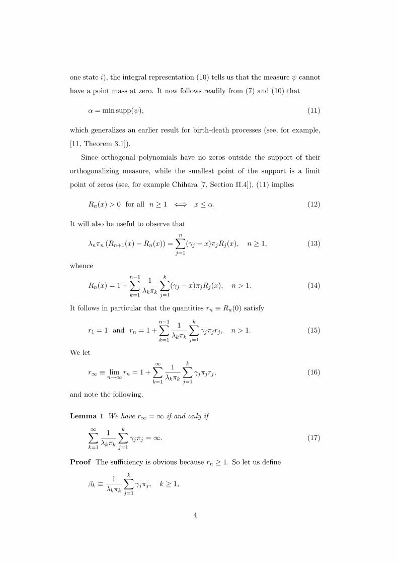
It follows in particular that the quantities rn ≡ Rn(0) satisfy

r1 = 1 and rn = 1 +n−1∑k=1

1λkπk

k∑j=1

γjπjrj , n > 1. (15)

We let

r∞ ≡ limn→∞

rn = 1 +∞∑

k=1

1λkπk

k∑j=1

γjπjrj , (16)

and note the following.

Lemma 1 We have r∞ = ∞ if and only if

∞∑k=1

1λkπk

k∑j=1

γjπj = ∞. (17)

Proof The sufficiency is obvious because rn ≥ 1. So let us define

βk ≡1

λkπk

k∑j=1

γjπj , k ≥ 1,

4

and assume that∑βk converges. Since rn is increasing in n we have

rn+1 = rn +1

λnπn

n∑j=1

γjπjrj ≤ rn(1 + βn), n ≥ 1,

so that

rn+1 ≤n∏

k=1

(1 + βk), n ≥ 1.

But∏

(1 + βk) and∑βk converge together, so we must have r∞ < ∞, as

required. 2

We conclude this section with representations for the extinction and eventual

extinction probabilities. Indeed, the forward equations tell us that

p′i0(t) =∑j∈C

γjpij(t), i ∈ C, t ≥ 0.

It follows that

τi(t) = pi0(t) =∑j∈C

γj

∫ t

0pij(u)du, i ∈ C, t ≥ 0, (18)

which, upon substitution of (10) and interchanging the integrals, leads to

τi(t) =∑j∈C

γjπj

∫ ∞

0(1− e−xt)Ri(x)Rj(x)

ψ(dx)x

, i ∈ C, t ≥ 0.

Letting t→∞ subsequently yields

τi =∑j∈C

γjπj

∫ ∞

0Ri(x)Rj(x)

ψ(dx)x

, i ∈ C, (19)

(by monotone convergence) and hence

τi(t) = τi −∑j∈C

γjπj

∫ ∞

0e−xtRi(x)Rj(x)

ψ(dx)x

, i ∈ C, t ≥ 0. (20)

The expression (19) will be evaluated in the next section, and τi(t) will be

studied in the Sections 4 and 5.

5

3 Eventual extinction probability

We note that by conditioning on the first event in X (or using the recurrence

relation (9) in (19)), the eventual extinction probabilities τi are readily seen to

satisfy the recurrence

(λi + µi + γi)τi = λiτi+1 + µiτi−1 + γi, i > 1,

(λ1 + γ1)τ1 = λ1τ2 + γ1.

In view of (19) with x = 0, it follows that τi may be expressed in terms of τ1

and ri ≡ Ri(0) as

1− τi = (1− τ1)ri, i ∈ C. (21)

Since {τi, i ∈ C} constitutes the smallest non-negative solution of (21) (cf.

Feller [14, p. 403]) we must have τi = 1 − ri/r∞, with the interpretation that

τi = 1 whenever r∞ = ∞. This result may also be obtained from Lemma 3.1 of

Brockwell [3], who studies eventual extinction probabilities in a more general

setting (see also Anderson [1, Section 9.2]). Considering Lemma 1 a simpler

criterion for certain extinction avails us in the setting at hand. Summarizing,

we conclude the following.

Theorem 2 If (17) is satisfied then τi = 1 for all i ∈ C, otherwise the eventual

extinction probabilities satisfy

τi = 1− rir∞

< 1, i ∈ C, (22)

with ri and r∞ given by (15) and (16), respectively.

In view of this result the condition (2) for non-explosiveness may be rephrased

as follows. A necessary and sufficient condition for non-explosiveness of X is

that either eventual extinction is certain or∞∑

n=1

1λnπn

n∑i=1

πi = ∞. (23)

As might be expected, the latter is precisely the condition for non-explosiveness

of X ∗ ≡ [X |T = ∞], the (pure birth-death) process one gets by setting γi = 0

for all i ∈ C (see [1, Section 8.1]).

6

4 Rate of convergence

In addition to accessibility of state 0 we will assume in this section that ab-

sorption at 0 is certain, that is, eventual extinction is certain and hence (17)

is satisfied. Pakes [26, p. 122] has observed (see also Elmes et al. [13]) that

the latter assumption is no restriction because if τi < 1 we can work with the

(Markov) process X ≡ [X |T < ∞], which has transition rates qij = qijτj/τi,

and transition probabilities pij(t) = pij(t)τj/τi. Here τ0 ≡ 1, and τi > 0 because

of our accessibility assumption. It follows that

τi(t) ≡ pi0(t) = pi0(t)/τi = τi(t)/τi → 1 as t→∞, i ∈ C.

We note from (20) that ξi(t) ≡ 1−τi(t) = Pi(T > t), the survival probability

at time t, can be represented in the form

ξi(t) =∑j∈C

γjπj

∫ ∞

0e−xtRi(x)Rj(x)

ψ(dx)x

, i ∈ C, t ≥ 0. (24)

In view of (11) (recall that ψ does not have an atom at 0) it is therefore tempting

to believe that α0 = α, but this is not true in general. Since 1 ≥ ξi(t) ≥ pii(t)

we do know, however, that

0 ≤ α0 ≤ α. (25)

This was observed already by Kingman [24, Theorem 8] and more recently by

Jacka and Roberts [19, (3.1.4)], whose example with strict inequalities in (25)

is encompassed in the setting which is described next.

Suppose the killing rates satisfy γi ≥ γ > 0 for all i ∈ C. Then we may look

upon the process X as a birth-death process with killing X , say, with rates λi ≡

λi, µi ≡ µi and γi ≡ γi−γ, which is subject to an additional killing event taking

place at rate γ. Evidently, absorption at 0 of X is certain. By conditioning on

the time of the additional killing event we have pij(t) = e−γtpij(t), i, j ∈ C,

and hence

α(X ) = γ + α(X ). (26)

By conditioning again we also obtain

ξi(t) = e−γt(1− τi(t)) = e−γt(1− τi) + e−γt(τi − τi(t)), i ∈ C, t ≥ 0,

7

where τi(t) is the extinction probability at time t of the process X and τi its

limit as t→∞. Hence

α0(X ) =

γ if τ1 < 1

γ + α0(X ) if τ1 = 1.(27)

It follows that strict inequalities prevail in (25) when τ1 < 1 and α(X ) > 0. We

note in addition that the calculation of α0(X ) is reduced to the calculation of

α0(X ) if τ1 = 1.

It has been shown in [19] (in a more general setting and implicitly assuming

certain absorption) that we have α0 = α if only finitely many γi’s are positive,

which is also obvious from the representation (24). A more general result is the

following.

Theorem 3 If α > 0 and eventual extinction is certain, then we have∑j∈C

γjπjRj(α) = α∑j∈C

πjRj(α), (28)

and α0 = α whenever either sum in (28) converges.

Proof Recalling that Rj(α) > 0, and using an argument similar to that in the

proof of [10, Theorem 4.1] it is not difficult to show with (10) that, if α > 0,

qj ≡ limt→∞

pij(t)∑k∈C pik(t)

=πjRj(α)∑

k∈C πkRk(α), j ∈ C, (29)

which is to be interpreted as 0 if the sum diverges. On the other hand, since

extinction is certain we have∑

j∈C pij(t) = ξi(t), and hence we may use the

representation (24) to calculate qj in a similar fashion, yielding

qj = limt→∞

pij(t)ξi(t)

=απjRj(α)∑

k∈C γkπkRk(α), j ∈ C, (30)

again with the interpretation 0 if the sum diverges. Since the two limits must be

equal (28) must hold good. Moreover, if either sum in (28) converges, then qj >

0 (and (29) tells us that, actually, {qj , j ∈ C} constitutes a proper distribution).

Evidently (see also [19, Theorem 3.3.2 (ii)]), the latter is a sufficient condition

for α0 = α. 2

8

Remark Theorem 3 generalizes part of the Lemma in Good [15] (see also

[10, Theorem 3.2]), which concerns pure birth-death processes. When γi > 0

for infinitely many states i the situation differs essentially from the pure birth-

death setting in that we may have α > 0 and divergence of the series in (28)

simultaneously. If either series in (28) converges then the quantities qj of (29)

(or (30)) constitute a quasi-stationary distribution (see, for example, Pakes [26]).

In this case we also have

α0 = α = − limt→∞

1t

log Pi(T > t)

(see, [26, Lemma 2.1]).

If α0 = α, then the problem of determining α0 can be reduced to that of finding

the decay parameter in a pure birth-death process, for which many results are

available (see [5], [6], [9], [11], [16], [22], [23], [27], [28], [29]). Indeed, define

X ≡ {X(t), t ≥ 0} to be the birth-death process on C with birth and death

rates

λi ≡ λiri+1

riand µi+1 ≡ µi+1

riri+1

, i ∈ C, (31)

respectively, where ri ≡ Ri(0). Letting µ1 = µ1 = 0, it is easy to see from (31)

and (9) that

λiµi+1 = λiµi+1 and λi + µi = λi + µi + γi, i ∈ C.

By [12, Theorem 1], this implies that there are constants σij > 0 such that

pij(t) = σij pij(t), i, j ∈ C, t ≥ 0,

with pij(t) denoting the transition probabilities of X . (In the terminology of

[25] the processes X and X are similar). Consequently, X and X have the same

decay parameter.

5 Bounds for the survival probability

To obtain bounds for ξi(t) ≡ Pi(T > t), the survival probability at time t,

we choose the approach used in [27] - [29] for pure birth-death processes (see

9

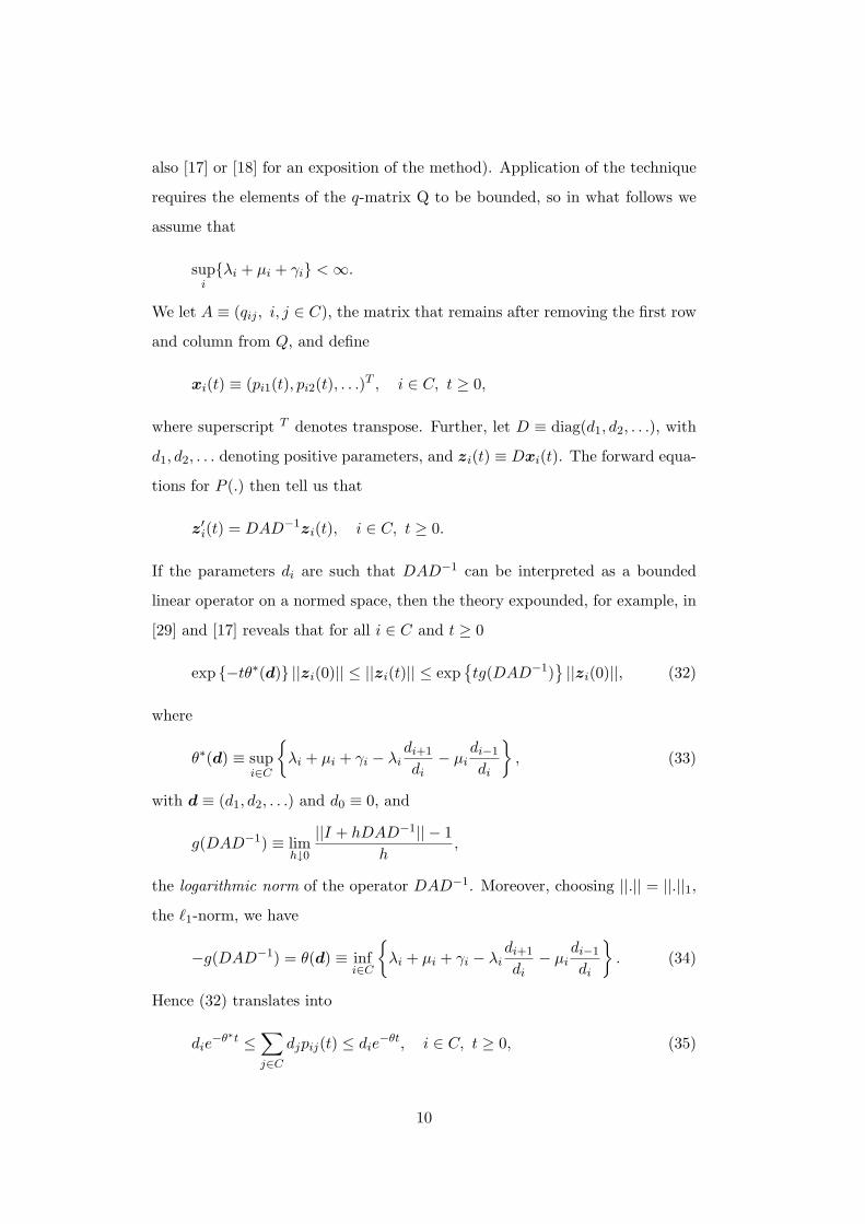
also [17] or [18] for an exposition of the method). Application of the technique

requires the elements of the q-matrix Q to be bounded, so in what follows we

assume that

supi{λi + µi + γi} <∞.

We let A ≡ (qij , i, j ∈ C), the matrix that remains after removing the first row

and column from Q, and define

xi(t) ≡ (pi1(t), pi2(t), . . .)T , i ∈ C, t ≥ 0,

where superscript T denotes transpose. Further, let D ≡ diag(d1, d2, . . .), with

d1, d2, . . . denoting positive parameters, and zi(t) ≡ Dxi(t). The forward equa-

tions for P (.) then tell us that

z′i(t) = DAD−1zi(t), i ∈ C, t ≥ 0.

If the parameters di are such that DAD−1 can be interpreted as a bounded

linear operator on a normed space, then the theory expounded, for example, in

[29] and [17] reveals that for all i ∈ C and t ≥ 0

exp {−tθ∗(d)} ||zi(0)|| ≤ ||zi(t)|| ≤ exp{tg(DAD−1)

}||zi(0)||, (32)

where

θ∗(d) ≡ supi∈C

{λi + µi + γi − λi

di+1

di− µi

di−1

di

}, (33)

with d ≡ (d1, d2, . . .) and d0 ≡ 0, and

g(DAD−1) ≡ limh↓0

||I + hDAD−1|| − 1h

,

the logarithmic norm of the operator DAD−1. Moreover, choosing ||.|| = ||.||1,

the `1-norm, we have

−g(DAD−1) = θ(d) ≡ infi∈C

{λi + µi + γi − λi

di+1

di− µi

di−1

di

}. (34)

Hence (32) translates into

die−θ∗t ≤

∑j∈C

djpij(t) ≤ die−θt, i ∈ C, t ≥ 0, (35)

10

where θ ≡ θ(d) and θ∗ ≡ θ∗(d). As an aside we note that θ(d) = θ∗(d) = x

if and only if di = cRi(x) for some constant c, as can easily be seen from the

recurrence relation (9). It follows in particular that∑j∈C

Rj(x)pij(t) = Ri(x)e−xt, i ∈ C, t ≥ 0, (36)

from which the representation (10) may be derived (cf. Karlin and McGregor

[20, Section I.2]).

Since

ξi(t) ≡ Pi(T > t) =∑j∈C

pij(t),

the inequalities (35) immediately give us the following bounds for the extinction

probability ξi(t).

Theorem 4 (i) Let dj ≥ 1 for all j ∈ C and θ ≡ θ(d) as in (34), then

ξi(t) ≤ die−θt, i ∈ C, t ≥ 0. (37)

(ii) Let dj ≤ 1 for all j ∈ C and θ∗ ≡ θ∗(d) as in (33), then

ξi(t) ≥ die−θ∗t, i ∈ C, t ≥ 0. (38)

Note that eventual extinction must be certain when dj ≥ 1 for all j ≥ 1 and

θ(d) > 0.

Corollary 5 If the constants µ ≥ 0 and a ≥ 0 are such that

µ < µj+1 and a ≤ µ+ γj −λjµ

µj+1 − µ, j = 1, 2, . . . ,

then

ξi(t) ≤ e−ati∏

j=1

µj+1

µj+1 − µ, i ∈ C, t ≥ 0. (39)

Proof Choosing d1 = 1 and dj+1/dj = µj+1/(µj+1 − µ) for j ≥ 1, we have

dj ≥ 1 and

θ(d) = infj∈C

{µ+ γj −

λjµ

µj+1 − µ

},

so that the conditions of Theorem 4 (i) are satisfied. Substitution in (37) gives

the result. 2

11

Taking µ = 0 it follows in particular that ξi(t) ≤ e−at if a ≤ inf{γj}, as we had

observed already by a different argument in the previous section.

If α, the decay parameter of X in C, is known, then the following corollary

might be useful. Recall that Rj(α) > 0 by (12).

Corollary 6 If 0 ≤ Rmin < Rj(α) < Rmax ≤ ∞ for all j then

Ri(α)Rmax

e−αt < ξi(t) <Ri(α)Rmin

e−αt, i ∈ C, t ≥ 0, (40)

where the left-hand (right-hand) side should be interpreted as zero (infinity) if

Rmax = ∞ (Rmin = 0).

Proof We have noticed already that letting dj = cRj(x) for some constant

c gives us θ(d) = θ∗(d) = x. Hence, if Rj(α) > Rmin > 0 for all j, then

the conditions of Theorem 4 (i) are satisfied if we choose a = α and dj =

Rj(α)/Rmin, and substitution in (37) gives the upper bound. On the other

hand, if Rj(α) < Rmax < ∞ for all j, then the conditions of Theorem 4 (ii)

are satisfied if we choose a = α and dj = Rj(α)/Rmax, and substitution in (38)

gives the lower bound. 2

Under certain circumstances (35) may lead to other bounds for ξi(t). For ex-

ample, suppose that γi > 0 for all i ∈ C, and choose di = γi in (34) – (35), so

that

γie−θ∗t ≤

∑j∈C

γjpij(t) ≤ γie−θt, i ∈ C, t ≥ 0,

where θ ≡ θ(γ), θ∗ ≡ θ∗(γ) and γ ≡ (γ1, γ2, . . .). If θ > 0 we obtain, in view of

(18), for ξi(t) ≡ 1− τi(t) the bounds

1− γi

θ

(1− e−θt

)≤ ξi(t) ≤ 1− γi

θ∗

(1− e−θ∗t

), i ∈ C, t ≥ 0. (41)

At the other extreme end, suppose that γi = 0 for i > 1, that is, we are

dealing with a pure birth-death process. Now choose di ≤ d1 for all i in (34) –

(35), and suppose θ ≡ θ(d) > 0. Then we have

γ1pi1(t) ≤γ1

d1

∑j∈C

djpij(t) ≤ γ1di

d1e−θt, i ∈ C, t ≥ 0,

12

by (35), and hence, by (18) again,

ξi(t) ≥ 1− γ1

θ

di

d1

(1− e−θt

), i ∈ C, t ≥ 0. (42)

We conclude this section by noting that the result (35) can easily be general-

ized to non-homogeneous processes. Specifically, let X be birth-death processes

with killing with time-dependent birth rates λn(t), death rates µn(t), and killing

rates γn(t). Then, under appropriate boundedness conditions and for all i ∈ C

and t ≥ 0,

di exp{−

∫ t

0θ∗(u)du

}≤

∑j∈C

djpij(t) ≤ di exp{−

∫ t

0θ(u)du

}, (43)

where

θ(d, t) ≡ infi∈C

{λi(t) + µi(t) + γi(t)− λi(t)

di+1

di− µi(t)

di−1

di

}, t ≥ 0, (44)

and

θ∗(d, t) ≡ supi∈C

{λi(t) + µi(t) + γi(t)− λi(t)

di+1

di− µi(t)

di−1

di

}, t ≥ 0.(45)

The corresponding generalisations of Theorem 4 and Corollary 5 are straight-

forward.

6 Example

Interesting cases arise if γi > 0 for infinitely many states i, while γi is not

constant for all i. We will analyse a simple example satisfying these conditions,

namely the process with transition rates

λi ≡ λ, µi ≡ µI{i>1} and γi ≡ γI{i>1}, i ∈ C, (46)

for some constants λ > 0, µ > 0 and γ > 0, where IE denotes the indicator

function of an event E. It is easily seen that (17) is satisfied so that extinction

is certain. The polynomials Rn of (9) satisfy the recurrence relation

λRn+1(x) = (λ+ µ+ γ − x)Rn(x)− µRn−1(x), n > 1,

λR2(x) = λ− x, R1(x) = 1,(47)

13

which, by the transformation

Sn(x) ≡ (−1)n

(λ

µ

)n/2

Rn+1(λ+ µ+ γ + 2x√λµ), n ≥ 0, (48)

reduces to

Sn(x) = 2xSn−1(x)− Sn−2(x), n > 1,

S1(x) = 2x+ η, S0(x) = 1,(49)

where

η ≡ µ+ γ√λµ

. (50)

The polynomials Sn can be represented as

Sn(x) = Un(x) + ηUn−1(x), n ≥ 1, (51)

where Un(x) denote the Chebysev polynomials of the second kind. The latter

satisfy the recurrence

Un(x) = 2xUn−1(x)− Un−2(x), n > 1,

U1(x) = 2x, U0(x) = 1,(52)

and may be represented as

Un(x) =zn+1 − z−(n+1)

z − z−1, x =

12(z + z−1), n ≥ 0. (53)

It will be useful to observe that

Un(x) = (−1)nUn(−x) and Un(1) = n+ 1. (54)

By appropriately transforming the orthogonalizing measure for {Sn(x)} given

in Chihara [7, p. 205] we can conclude that the polynomials Rn are orthogonal

with respect to a measure which consists of a positive density on the interval(λ+ µ+ γ − 2

√λµ, λ+ µ+ γ + 2

√λµ

),

and, if µ+ γ >√λµ, an atom at the point λγ/(µ+ γ). Since

λγ

µ+ γ= λ+ µ+ γ −

√λµ

(η + η−1

), (55)

it thus follows from (11) that

α = λ+ µ+ γ −

2√λµ if µ+ γ ≤

√λµ

√λµ

(η + η−1

)if µ+ γ ≥

√λµ.

(56)

14

We next wish to determine the value of α0. To this end we will not try to

employ (24), but rather argue as follows. Let Ea denote an exponentially dis-

tributed random variable with mean a−1, and B a random variable representing

the busy period in an M/M/1 queueing system with arrival rate λ and service

rate µ. (If λ > µ the distribution of B is defective.) A little reflection then

shows that, if the initial state is 1, the extinction time T may be represented as

T = Eλ + EγI{Eγ≤B} + (B + T ∗)I{Eγ>B},

where T and T ∗ are independent but identically distributed. It follows that

τ(s)≡ E[e−sT ] = E[e−sT I{Eγ≤B} + e−sT I{Eγ>B}

]= E

[e−sEλ

(e−sEγ I{Eγ≤B} + e−s(B+T ∗)I{Eγ>B}

)]=

λ

λ+ s

(E

[e−sEγ I{Eγ≤B}

]+ τ(s)E

[e−sBI{Eγ>B}

]),

so that

(λ+ s− λE

[e−sBI{Eγ>B}

])τ(s) = λE

[e−sEγ I{Eγ≤B}

]. (57)

A little algebra reveals that

E[e−sEγ I{Eγ≤B}

]=

γ

γ + s(1− B(γ + s)),

and

E[e−sBI{Eγ>B}

]= B(γ + s),

where B(s) ≡ E[e−sB]. Substitution of these results in (57) gives us

τ(s) =γ(λ− λB(γ + s))

(γ + s)(λ+ s− λB(γ + s)). (58)

It is well known (see, for instance, Cohen [8, Eq. (II.2.31)]) that

B(s) =12λ

(λ+ µ+ s−

√(λ+ µ+ s)2 − 4λµ

),

which, upon substitution in (58) and some algebra, leads to

τ(s) =γ

(s2 + (λ+ µ+ γ)s+ 2λγ − s

√(λ+ µ+ γ + s)2 − 4λµ

)2(γ + s)(λγ + (µ+ γ)s)

. (59)

15

By inverting this expression we can obtain an explicit formula for τ1(t), the

extinction time distribution when the initial state is 1. At this point, however,

we are interested only in α0 – the rate of convergence of τ1(t) – which, apart from

a minus sign, equals the singularity of τ(s) which is closest to the imaginary

axis. Since the largest branch point at −γ− (√λ−√µ)2 is always smaller than

the pole at −γ it follows that α0 = γ or α0 = λγ/(µ+γ), depending on whether

λ ≥ µ+ γ or λ ≤ µ+ γ, respectively.

Collecting all our results we conclude the following.

Theorem 7 The process with transition rates (46) has rates of convergence α0

and α given by

α0 = α =λγ

µ+ γif λ ≤ µ+ γ,

α0 = γ < α =λγ

µ+ γif

√λµ ≤ µ+ γ < λ,

and

α0 = γ < α = γ +(√

λ−√µ)2

if µ+ γ <√λµ.

Observe that our findings are in accordance with the intuitive result that α0

must tend to zero as γ tends to zero.

It is interesting to establish how much of the information in Theorem 7 may

be obtained from Theorem 3. To this end we note that, by (3) and (46),

πn+1 =(λ

µ

)n

, n ≥ 0, (60)

so that, by (48),

πn+1Rn+1(x) = (−1)n

(λ

µ

)n/2

Sn

(x− λ− µ− γ

2√λµ

), n ≥ 0. (61)

Hence, it follows after some algebra from (51), (53) and (54) that, for n ≥ 0,

πn+1Rn+1(α) =

(1 + (1− η)n)

(λ

µ

)n/2

if µ+ γ ≤√λµ(

λ

µ+ γ

)n

if µ+ γ ≥√λµ.

(62)

Since√λµ < µ + γ if λ < µ + γ, while λ > µ if λ ≥ µ + γ, we conclude that

the series in (28) converge if and only if λ < µ+ γ. Hence, Theorem 3 tells us

that α0 = α if λ < µ+ γ. In the opposite case Theorem 3 does not help us.

16

By extending the method by which we have calculated τ(s) we can obtain

the Laplace-Stieltjes transform of the extinction time distribution when the

initial state is any state i ∈ C rather than 1. By inversion we can therefore,

in principle at least, calculate τi(t), and hence ξi(t). But the procedure is

cumbersome so it is of interest to apply the methodology of Section 5 to the

present example. For instance, choosing d1 = 1 and

dj+1 =(

µ

µ+ γ

)j

, j ≥ 1,

in (33) gives us θ∗ = λγ/(µ+ γ) and hence, by Theorem 4 (ii),

ξi(t) ≥(

µ

µ+ γ

)i−1

exp{−λγtµ+ γ

}, i ∈ C, t ≥ 0. (63)

This is also the bound produced by Corollary 6 when µ+ γ ≥√λµ. In the case

µ+ γ <√λµ Corollary 6 yields a lower bound which we will not spell out, but

improves upon (63) for t sufficiently large.

As an aside we finally note that ours is yet another example, next to the

examples in Pakes [26] and Bobrowski [2], showing that asymptotic remoteness,

that is,

limi→∞

pi0(t) = 0, t ≥ 0, (64)

is not necessary for the existence of a quasi-stationary distribution. Indeed, it

is obvious that (64) is not satisfied in the present setting, while, in view of (62)

and the Remark following Theorem 3, a quasi-stationary distribution does exist

when λ < µ+ γ.

References

[1] Anderson, W.J. (1991). Continuous-time Markov Chains. Springer, New

York.

[2] Bobrowski, A. (2004) Quasi-stationary distributions of a pair of Markov

chains related to time evolution of a DNA locus. Adv. Appl. Probab. 36,

56-77.

17

[3] Brockwell, P.J. (1986). The extinction time of a general birth and death

process with catastrophes. J. Appl. Probab. 23, 851-858.

[4] Chen, A., Pollett, P., Zhang, H. and Cairns, B. (2003). Uniqueness crite-

ria for continuous-time Markov chains with general transition structure.

Preprint.

[5] Chen, M.F. (1991). Exponential L2-convergence and L2-spectral gap for

Markov processes. Acta Math. Sinica (N.S.) 7, 19-37.

[6] Chen, M.F. (1996). Estimation of the spectral gap for Markov chains. Acta

Math. Sinica (N.S.) 12, 337-360.

[7] Chihara, T.S. (1978). An Introduction to Orthogonal Polynomials. Gordon

and Breach, New York.

[8] Cohen, J.W. (1982). The Single Server Queue, rev. ed. North-Holland,

Amsterdam.

[9] van Doorn, E.A. (1985). Conditions for exponential ergodicity and bounds

for the decay parameter of a birth-death process. Adv. Appl. Probab. 17,

514-530.

[10] van Doorn, E.A. (1991). Quasi-stationary distributions and convergence to

quasi-stationarity of birth-death processes. Adv. Appl. Probab. 23, 683-700.

[11] van Doorn, E.A. (2002). Representations for the rate of convergence of

birth-death processes. Theory Probab. Math. Statist. 65, 37-43.

[12] van Doorn, E.A. and Zeifman, A.I. (2004). Birth-death processes with

killing. Submitted.

[13] Elmes, S., Pollett, P. and Walker, D. (2000). Further results on the rela-

tionship between µ-invariant measures and quasi-stationary distributions

for absorbing continuous-time Markov chains. Math. Comput. Modelling

31, 107-113.

18

[14] Feller, W. (1967). An Introduction to Probability Theory and Its Applica-

tions, Vol. I, rev. ed. Wiley, New York.

[15] Good, P. (1968). The limiting behavior of transient birth and death pro-

cesses conditioned on survival. J. Aust. Math. Soc. 8, 716-722.

[16] Granovsky, B.L. and Zeifman, A.I. (1997). The decay function of nonho-

mogeneous birth-death processes, with applications to mean-field models.

Stochastic Process. Appl. 72, 105-120.

[17] Granovsky, B.L. and Zeifman, A.I. (2000). The N -limit of spectral gap of

a class of birth-death Markov chains. Appl. Stoch. Models Bus. Ind. 16,

235-248.

[18] Granovsky, B.L. and Zeifman, A.I. (2004). Nonstationary queues: estima-

tion of the rate of convergence. Queueing Syst. 46, 363-388.

[19] Jacka, S.D. and Roberts, G.O. (1995). Weak convergence of conditioned

processes on a countable state space. J. Appl. Probab. 32, 902-916.

[20] Karlin, S. and McGregor, J.L. (1957). The differential equations of birth-

and-death processes, and the Stieltjes moment problem. Trans. Amer.

Math. Soc. 85, 589-646.

[21] Karlin, S. and Tavare, S. (1982). Linear birth and death processes with

killing. J. Appl. Probab. 19, 477-487.

[22] Kartashov, N.V. (1998). Calculation of the exponential ergodicity exponent

for birth-death processes. Theory Probab. Math. Statist. 57, 53-60.

[23] Kijima, M. (1992). Evaluation of the decay parameter for some specialized

birth-death processes. J. Appl. Probab. 29, 781-791.

[24] Kingman, J.F.C. (1963) The exponential decay of Markov transition prob-

abilities. Proc. London Math. Soc. 13, 337-358.

19

[25] Lenin, R.B., Parthasarathy, P.R., Scheinhardt, W.R.W. and van Doorn,

E.A. (2000). Families of birth-death processes with similar time-dependent

behaviour. J. Appl. Probab. 37, 835-849.

[26] Pakes, A.G. (1995). Quasi-stationary laws for Markov processes: examples

of an always proximate absorbing state. Adv. Appl. Probab. 27, 120-145.

[27] Zeifman, A.I. (1991). Some estimates of the rate of convergence for birth

and death processes. J. Appl. Probab. 28, 268-277.

[28] Zeifman, A.I. (1995). On the estimation of probabilities for birth and death

processes. J. Appl. Probab. 32, 623-634.

[29] Zeifman, A.I. (1995). Upper and lower bounds on the rate of convergence

for nonhomogeneous birth and death processes. Stochastic Process. Appl.

59, 157-173.

20