Page 1
Extracting Secret Keys from Integrated Circuits
by
Daihyun Lim
Submitted to the Department of Electrical Engineering and ComputerScience
in partial fulfillment of the requirements for the degree of
Master of Science in Electrical Engineering and Computer Science
at the
MASSACHUSETTS INSTITUTE OF TECHNOLOGY
May 2004 Loe 2zoq4
© Massachusetts Institute of Technology 2004. All rights reserved.
Author ................... ........ ..'..... ..........................Department of Electrical Engineering and Computer Science
May 20, 2004
Certified by ........ ............ ..... ........ ....X
Srinivas DevadasProfessor of Electrical Engineering and Computer Science
Thesis Supervisor
Accepted by .........--.......................Arthur C. Smith
Chairman, Department Committee on Graduate StudentsARcHIVES
MASSACHUSETr S INSnTUTEOF TECHNOLOGY
JUL 2 6 2004
LIBRARIES
Page 3
Extracting Secret Keys from Integrated Circuits
by
Daihyun Lim
Submitted to the Department of Electrical Engineering and Computer Scienceon May 20, 2004, in partial fulfillment of the
requirements for the degree ofMaster of Science in Electrical Engineering and Computer Science
Abstract
Modern cryptographic protocols are based on the premise that only authorized par-ticipants can obtain secret keys and access to information systems. However, variouskinds of tampering methods have been devised to extract secret keys from widelyfielded conditional access systems such as smartcards and ATMs. As a solution,Arbiter-based Physical Unclonable Functions (PUFs) are proposed. This techniqueexploits statistical delay variation of wires and transistors across integrated circuits(ICs) in the manufacturing processes to build a secret key unique to each IC. Wefabricated Arbiter-based PUFs in custom silicon and investigated the identificationcapability, reliability, and security of this scheme. Experimental results and theoreti-cal studies show that a sufficient amount of variation exists across ICs. This variationenables each IC to be identified securely and reliably over a practical range of environ-mental variations such as temperature and power supply voltage. Thus, arbiter-basedPUFs are well-suited to build key-cards and membership cards that must be resistantto cloning attacks.
Thesis Supervisor: Srinivas DevadasTitle: Professor of Electrical Engineering and Computer Science
3
Page 5
Acknowledgments
This work was funded by Acer Inc., Delta Electronics Inc., HP Corp., NTT Inc., Nokia
Research Center, and Philips Research under the MIT Project Oxygen partnership.
First of all, I would like to extend my sincere gratitude to my advisor, Srinivas
Devadas, for his inspiring advice and encouragement from the beginning through the
end of this research. I have learned what research is and how fun it is from working
with him. I also greatly thank Marten van Dijk, the guru of mathematics, who is
always full of interesting ideas and ready to formulate and solve problems.
My gratitude also extends to all of Computation Structures Group people for their
support and encouragement. I would like to specially thank Blaise Gassend, who
answered many of my questions and provided me a Debian Linux environment, which
has played an important role in PUF experiments. I also appreciate Jaewook Lee for
his help in designing and fabricating test-chips for experiments in this thesis. Edward
Gookwon Suh provided me a cute thermometer that made it possible to measure the
temperature variation of PUFs. My old office-mate Prabhat Jain deserves special
credit for his advices about how to survive here from the beginning of my MIT life. I
warmly thank my current office-mate Charles O'Donnell, the excellent rower who is
better than any other woman in the world, and Michael Zhang, the enthusiastic pool
player who hates to lose every game, for their outstanding advices about writing.
I thank all of my friends who have made my life at MIT so enjoyable, especially
my girl-friend Jerin Gu.
Last, I would like to thank my mom for her love and encouragement.
5
Page 7
Contents
1 Introduction
1.1 Secure Storage of Secret Keys ......................
1.2 Random Functions as Secret Key Storage ................
1.3 Exploiting Process Variation in Silicon Manufacturing .
1.4 Organization ...............................
2 Physical Random Functions for Secret Key Storage
2.1 Definition of Physical Random Functions ................
2.1.1 Definition of One Way Functions ................
2.1.2 Definition of Physical Random Functions ............
2.2 Secret Key Storage ............................
2.2.1 Manufacturer Resistant PUFs ..................
2.2.2 Applications .
3 Arbiter-Based PUF
3.1 Delay-Based Authentication.
3.1.1 Statistical Delay Variation . . .
3.1.2 Measurement of Delays.
3.1.3 Generating Challenge-Response
3.2 Arbiter-Based PUF.
3.2.1 General Description .......
3.2.2 Switch Blocks and Delay Paths
3.2.3 Arbiter .
7
. . .
. . .
.air
Pairs
.. .
. . .
. . .
17
17
18
19
19
21
21
21
22
23
23
24
27
27
27
28
30
30
31
32
33
..............
..............
..............
..............
..............
..............
..............
..............
Page 8
3.3 Analysis and Characterization of Arbiter-Based PUF
3.3.1 Inter-chip Variation .
3.3.2
3.3.3
3.3.4
Reliability.
Performance .
Aging.
4 Modeling an Arbiter-Based PUF
4.1 Delay Model .
4.1.1 Linear Delay Model .
4.1.2 Non-Linear Delay Model
4.2 Estimation of Model Parameters
4.2.1 Estimation of si/a .....
4.2.2 Estimation of a/arp ....
4.2.3 Estimation of oax/ap using a
4.3 Experiments. ............
4.3.1 Estimation of si .......
4.3.2 Estimation of auA/Up ....
4.3.3 Estimation of Non-linearity
.................... . .38
. . . . . . . . . . . . . . . . . ... 40
. . . . . . . . . . . . . . . . . ... 40
43
. . . . . . . . . . . . . . . . . ... 44
. . . . . . . . . . . . . . . . . ... 44
. . . . . . . . . . . . . . . . . ... 45
. . . . . . . . . . . . . . . . . ... 46
. . . . . . . . . . . . . . . . . ... 46
. . . . . . . . . . . . . . . . . ... 48
Non-linear Delay Model ..... 53
55
55
56
57
59
59
64
4.4 Identification/Authentication Capability . . . . . . . . .
4.4.1 Inter-chip Variation and Environmental Variation
4.4.2 Identification/Authentication Capability.
5 Breaking an Arbiter-Based PUF
5.1 Attack Models .
5.1.1 Duplication.
5.1.2 Timing-Accurate Model Building ............
5.1.3 Software Model Building Attacks ............
5.2 Software Modeling Building Attack: Support Vector Machines
5.2.1 Additive Delay Model of a PUF Circuit .........
5.2.2 Support Vector Machines .................
5.3 Experiments. ...........................
69
. . 69
. . 70
. . 70
.. 72
. . 72
. . 73
.. 75
.. 77
8
........ . V35
35
Page 9
5.3.1
5.3.2
Experiments using a FPGA implementation ..........
Experiments using a Custom Silicon Implementation .....
6 Strengthening an Arbiter-Based PUF
6.1 Secure Delay Models ...............
6.1.1 Feed-forward Arbiter Approach .....
6.1.2 Non-linear Arbiter-based PUF Approach
6.2 Reliability .....................
6.2.1 Distribution of Random Challenges . . .
6.2.2 Robust Challenges ............
7 Conclusion
7.1 Ongoing and Future Work .................
7.1.1 Reliable Secret Sharing with PUFs . . . . . . . .
7.1.2 Reconfigurable PUFs using Non-volatile Storage .
7.1.3 PUF-based Physical Random Number Generators
A Parameter Estimation
B Properties of Q(x)
9
77
78
81
. . . . . . . . . . . . .82
. . . . . . . . . . . . .82
. . . . . . . . . . . . .91
. . . . . . . . . . . . .94
. . . . . . . . . . . . .95
. . . . . . . . . . . . .96
103
103
103
105
106
109
113
Page 11
List of Figures
2-1 The general model of identification system based on a PUF key-card. 25
2-2 The model of PUF-based membership cards ............... 26
3-1 The direct delay measurement using a ring oscillator circuit ...... 28
3-2 The relative delay measurement using a comparator circuit ...... 29
3-3 The structure of an arbiter-based PUF (basic arbiter scheme) ..... 31
3-4 Implementation of a switch component .................. 32
3-5 A simple transparent data latch primitive and its signal transitions . 33
3-6 Compensating for the arbiter skew by fixing the most significant bits
of a challenge vector ................... ........ 34
3-7 The density function of the random variable p = Prob(R(c) = 1) . . . 36
3-8 The density of the inter-chip variation yi,j for a number of PUF pairs. 38
3-9 The inter-chip variation of the PUFs from a single wafer and across
wafers .................................... 39
3-10 The variation of PUF responses subjected to temperature and supply
voltage changes. ................... . . . . . . . . . . . 40
3-11 The aging effect on an arbiter-based PUF for 25 days .......... 41
4-1 Accuracy intervals and their overlapping region ............. 52
4-2 Estimated skew parameters and their accuracy intervals from indepen-
dent experiments .............................. 55
4-3 Estimated up and their accuracy intervals from independent experiments. 56
4-4 Comparison of pt-R' curves depending on the existence of non-linear
noise.. ..................................... 58
11
Page 12
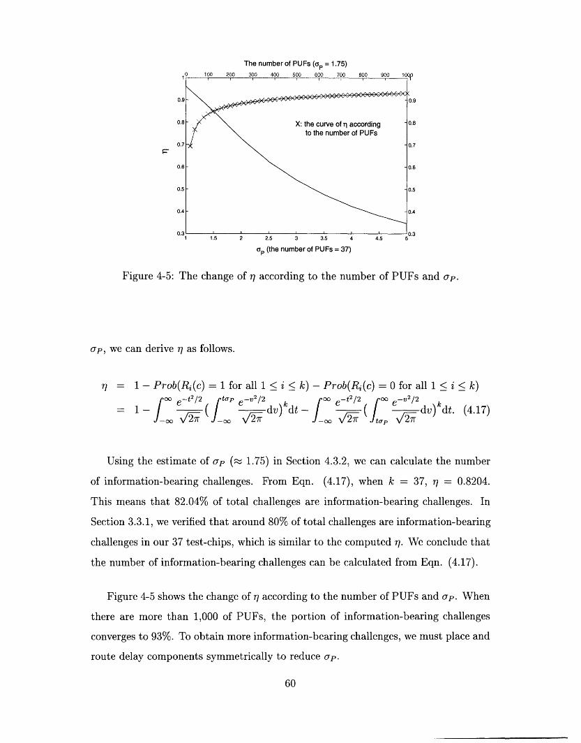
4-5 The change of rj according to the number of PUFs and p. ....... 60
4-6 The change of T according to the number of the stages in delay paths. 63
5-1 The notations of delay segments in each stage .............. 73
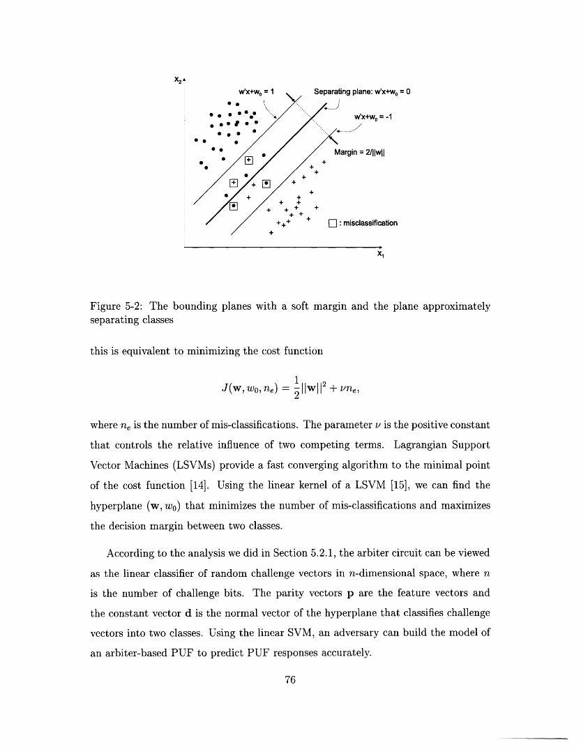
5-2 The bounding planes with a soft margin and the plane approximately
separating classes ............................. 76
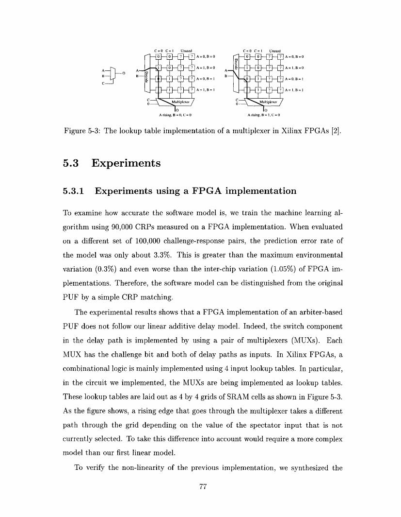
5-3 The lookup table implementation of a multiplexer in Xilinx FPGAs [2]. 77
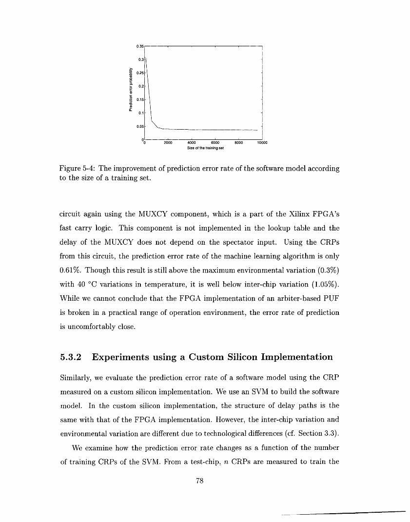
5-4 The improvement of prediction error rate of the software model ac-
cording to the size of a training set .................... 78
6-1 Adding unknown challenge bits using feed-forward arbiters (feed-forward
arbiter scheme). ................ .. . . . . . . . . . . . 82
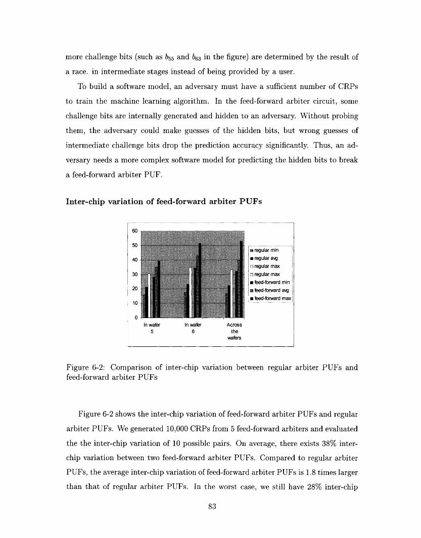
6-2 Comparison of inter-chip variation between regular arbiter PUFs and
feed-forward arbiter PUFs ................... ..... 83
6-3 Estimates of up and their accuracy intervals for feed-forward arbiter
PUFs .................................... 85
6-4 Temperature and power supply voltage variations of feed-forward ar-
biter PUFs. ................................ 86
6-5 The feed-forward arbiter circuit with one feed-forward stage ...... 87
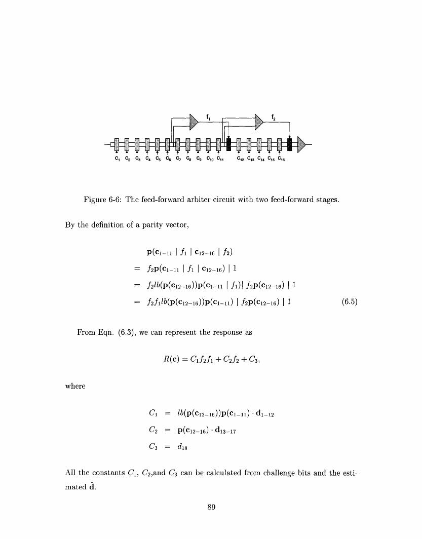
6-6 The feed-forward arbiter circuit with two feed-forward stages. .... 89
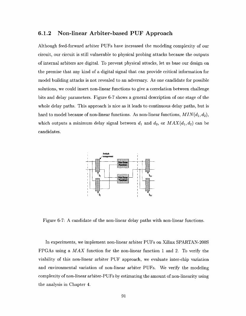
6-7 A candidate of the non-linear delay paths with non-linear functions. . 91
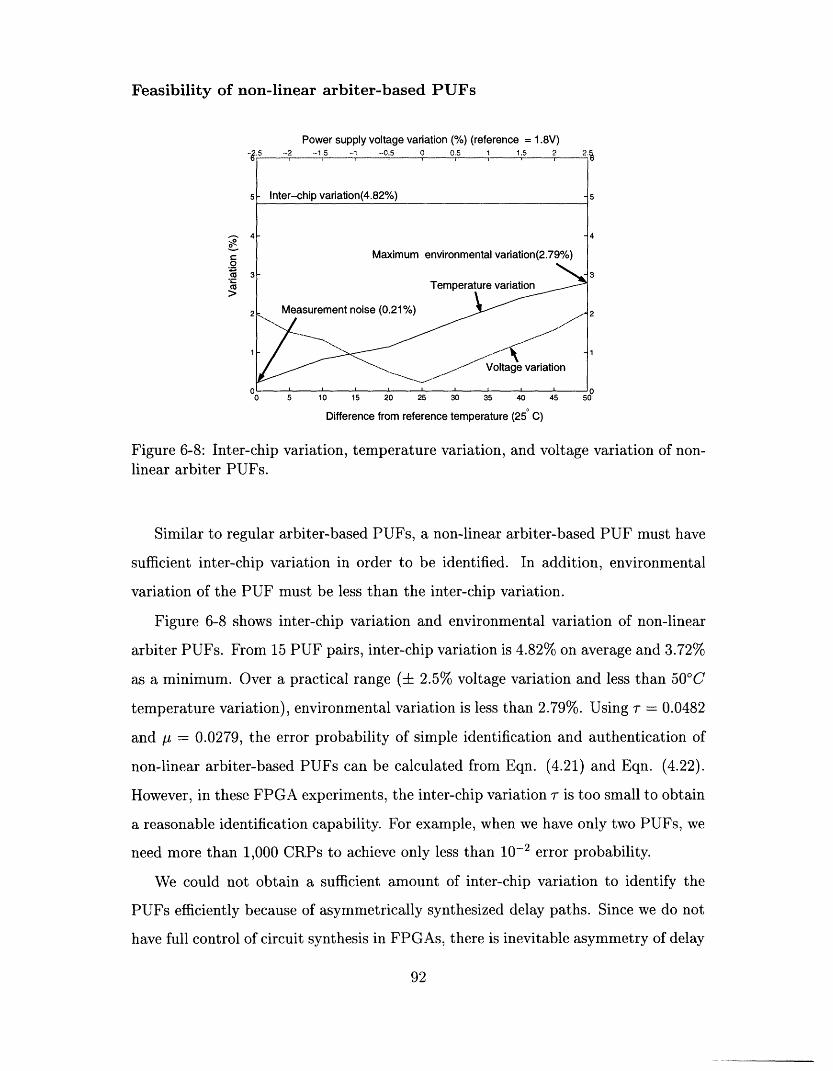
6-8 Inter-chip variation, temperature variation, and voltage variation of
non-linear arbiter PUFs .......................... 92
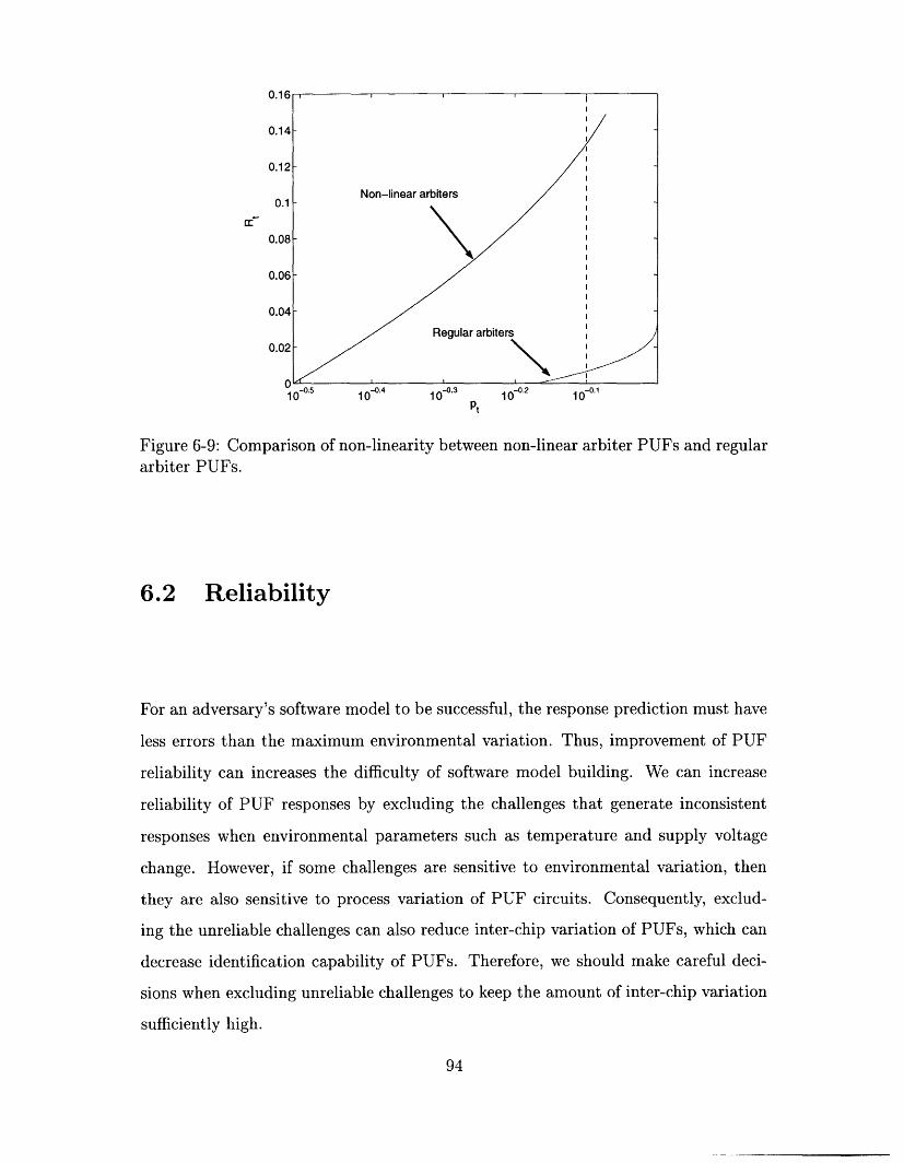
6-9 Comparison of non-linearity between non-linear arbiter PUFs and reg-
ular arbiter PUFs. ............................ 94
6-10 Distribution of random challenges according to A(c) .......... 96
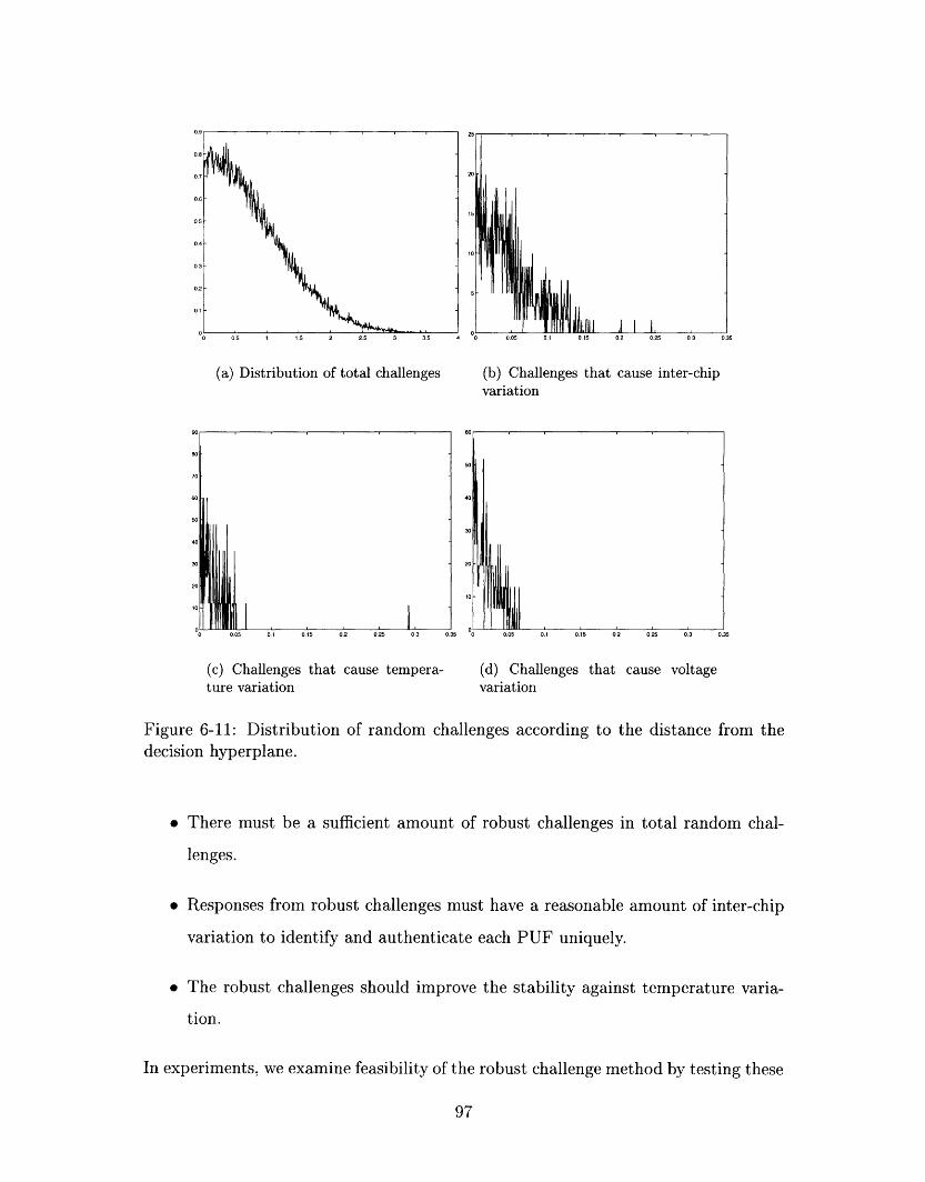
6-11 Distribution of random challenges according to the distance from the
decision hyperplane. ............................ 97
6-12 Experimental results of MIN(dl, d 2) at different temperature. .... 102
7-1 The circuit diagram of a reconfigurable arbiter-based PUF ....... 106
12
Page 13
7-2 The density function of the random variable k, where k is the number
of s out of 200 repetitive measurements ................. 107
13
Page 15
List of Tables
3.1 The transition table of a transparent data latch with an inverted gate 33
4.1 Measurement noises in the different number of stages .......... 64
6.1 Improvement of reliability using the robust challenges in 15 repetitive
measurements ................................ 98
6.2 Improvement of reliability using the robust challenges in ±1.5% voltage
variation .................................. 99
6.3 Improvement of reliability using the robust challenges to repetitive
measurements and voltage variation. .................. 100
15
Page 17
Chapter 1
Introduction
1.1 Secure Storage of Secret Keys
For many emerging applications that need exceptional security in identifying and
authenticating users, such as intellectual property protection, Pay-TVs, and ATMs,
system security is based on the protection of secret keys. Malicious users can imper-
sonate authorized users when the secret key is uncovered. Thus, private information
storage devices, such as smartcards, provide active logical controls for the protection
of secret information against logical and physical tampering attacks.
However, recently developed physical tampering methods such as micro-probing,
laser cutting, glitch attacks, and power analysis have made it possible to extract dig-
italized secret information and compromise widely fielded conditional access systems.
For example, an adversary can remove a smartcard package and reconstruct the lay-
out of the circuit using chemical and optical methods. He can even read out the
information stored in non-volatile memories such as EEPROMs and NVRAMs [13].
Researchers have invented various protection mechanisms to prevent invasive phys-
ical attacks. For example, we can introduce additional metalization layers that form
a sensor mesh above the actual circuit [13]. The sensor mesh technique has been used
in some commercial smartcard CPUs, such as the ST16SF48A and in some battery-
buffered SRAM security processors, such as the DS5002FPM and DS1954. Using
a sensor mesh, any interruption and short-circuit can be monitored while power is
17
Page 18
available, and a laser cutter or selective etching access to bus lines can be prevented.
Though a tamper-sensing environment can cause difficulty for the adversary, the sen-
sor mesh cannot prevent the extraction of hard-wired information in a circuit when
the power is off. However, it can erase keys stored in non-volatile memory as soon as
tampering is detected.
Instead of using vulnerable hard-wired secret keys, we can exploit alternative
circuit parameters that are resistant to physical attacks on the premise that the
parameters can be converted into digital secret keys. Electrical properties such as
signal propagation delays, threshold voltages, and power consumption form good
candidates thank to their intrinsic randomness. In this thesis, we show how to build
secure storage of secret keys based on propagation delays in ICs.
1.2 Random Functions as Secret Key Storage
Recently, the randomness of functions has attracted much attention for its crypto-
graphic uses. The notion of pseudo-random functions based on computational com-
plexity is presented in [11]. The idea of using random functions as secure storage of
secret keys is discussed in [10]. Though pseudo-random functions are cryptographi-
cally strong against logical attacks, physical implementations of random functions are
still vulnerable to duplication of the secret keys by sophisticated reverse engineering.
Therefore, instead of computational complexity, using randomness in physical
materials can give a viable solution. As an example, the concept of Physical One-
Way Functions (POWFs) has been introduced in [18]. In this work, Pappu et. al.
show that the mesoscopic physics of coherent transport through a disordered medium
can be used to allocate and authenticate unique identifiers by physically reducing the
medium's micro-structure to a fixed-length string of binary digits. This POWF can
be used to build a random function that keeps a logical strength of a pseudo-random
function [11]. These physical random functions are strong against physical attacks
because an adversary is not in control of heterogeneous materials that hold secret
information.
18
Page 19
1.3 Exploiting Process Variation in Silicon Manu-
facturing
Silicon can be a good candidate of a base material to build physical random functions.
Gassend et. al. have introduced silicon physical random functions (also called Phys-
ical Unclonable Functions or PUFs for short) [8]. A PUF is based on the intrinsic
random process variation in the manufacturing of ICs. While ICs can be reliably mass-
manufactured to have identical digital functionalities, each IC can also be uniquely
characterized due to inherent manufacturing variation. Since the responses of the
PUF are designed to be sensitive to delay variation, process variation of transistors
and wires delays across ICs makes the response pattern of each PUF unique. Thus,
we can identify and authenticate each IC reliably by observing the PUF responses.
Since process variation is largely beyond the manufacturers' control, it is im-
possible for an adversary to make identical copies of a PUF. Moreover, since the
manufacturing variation is small compared to other measurable circuit parameters,
characterizing PUFs by probing internal propagation delays is an arduous task.
In this work, we propose a novel architecture, an arbiter-based PUF. By utilizing
a differential structure, this approach makes the PUFs more reliable against envi-
ronmentally induced noise. We thoroughly investigate the identification capability,
reliability and security of this approach in this thesis. We develop a theoretical model
of delay variation to estimate the feasibility of this approach in the mass-production of
ICs. PUF test-chips were fabricated using a TSMC 0.18 ,/m process. Using the test-
chips, we estimate the model parameters and verify the correctness of the theoretical
model. We also study the reliability of an arbiter-based PUF approach. Lastly, we
propose alternative architectures to improve the security of the arbiter-based PUFs.
1.4 Organization
This thesis is structured as follows. Chapter 2 defines physical random functions,
describes manufacture resistance of PUFs, and gives a general overview of PUF sys-
19
Page 20
tems.
Chapter 3 introduces the notion of delay-based authentication and a detailed
circuit implementation of arbiter-based PUFs. Furthermore, we show experimental
results for silicon PUFs implemented in custom silicon, and analyze the important
characteristics of PUFs such as inter-chip variation, measurement noise and environ-
mental noise. We also measure the performance and an aging effect in arbiter-based
PUFs.
Chapter 4 details the statistical model of an arbiter-based PUF circuit. We provide
an appropriate delay model of a PUF circuit and estimate model parameters. Based
on the model, we examine theoretical identification capability of arbiter-based PUFs.
We calculate the required number of measurements to identify billions of PUFs with
negligible probability of error. Moreover, we propose a parameter estimation method
to verify the accuracy of the model based on experimental results.
Chapter 5 studies the vulnerability of arbiter-based PUFs against possible attack
models. We provide a representation of arbiter responses as a linear function of
challenges and delay segments. Based on the linear model, we investigate a machine
learning algorithm, a Support Vector Machine (SVM), which can be trained by a small
amount of challenge-response pairs to predict responses of given random challenges.
We conclude that a software model building approach is critical to the security of
arbiter-based PUFs.
Chapter 6 suggests alternative types of arbiter-based PUFs for which it is more
difficult to build a software model by adding non-linearity in delay paths. From
our experiments, we evaluate each PUF's identification capabilities and estimate the
amount of non-linearity of the delay model using the method in Chapter 4. The
increased amount of non-linearity creates difficulty in model building for the new
arbiters.
Finally, Chapter 7 concludes the thesis and presents ideas for future work such as
reconfigurable PUFs and a PUF-based random number generator. We also present a
reliable secret sharing method using PUFs.
20
Page 21
Chapter 2
Physical Random Functions for
Secret Key Storage
Pseudo Random Functions (PRFs) have attracted attention in modern cryptogra-
phy. Because of their intriguing properties such as indexing, poly-time evaluation,
and pseudo-randomness, PRFs have been used in various cryptographic applications
[10], in particular, user identification and authentication. Though PRFs are crypto-
graphically strong, sophisticated physical attacks can still break the PRF circuit to
extract sensitive data.
In this chapter, we define a Physical Unclonable Function (PUF), which is con-
structed based on the randomness of physical materials to prevent physical attacks
while keeping the cryptographic strength of the PRFs. As applications, we present a
secure key-card system and Unclonable membership card system that are based on
the existence of PUFs.
2.1 Definition of Physical Random Functions
2.1.1 Definition of One Way Functions
Modern cryptography is based on the gap between efficient encryption for legitimate
users and the computational infeasibility of decryption. Thus, a cryptographic al-
21
Page 22
gorithm requires available primitives with special kinds of computational hardness
properties. A one-way function is a basic primitive in the modern cryptographic sys-
tem. Informally, a function is one-way if it is easy to compute but hard to invert. By
"easy", we mean that the function can be computed using a probabilistic polynomial
time (PPT) algorithm, and by "hard" that there is no PPT algorithm to invert it
with greater than "negligible" probability.
Here is the formal definition of one-way functions.
Definition 2.1.1. A function f: 0, 1* - ({0, 1)* is called strongly one-way if the
following two conditions hold.
* Easy to compute: There exists a deterministic polynomial time algorithm A
such that on input x, A outputs f(x) (that is, A(x) = f(x)).
* Hard to invert: For every probabilistic polynomial time algorithm A', every
polynomial P, and all sufficiently large n
Pr(A'(f(y)) E f-l(f(y))) < '
The second condition means that the probability that algorithm A' will find an
inverse of y under f is negligible. The strong one-way functions above require that
any efficient inverting algorithm has negligible success probability. Weak one-way
functions require only that all efficient algorithms fail with some non-negligible prob-
ability.
If the size of the output, i.e., f(x), is always fixed, regardless of the size of the
input x, then the function f(x) is called a one-way hash function. This definition of
one-way hash function will be used as a template when we define physical random
functions in the next section.
2.1.2 Definition of Physical Random Functions
We can construct a poly-random collection of functions that cannot be distinguished
from pure random functions based on the existence of one-way functions [11]. Instead
22
Page 23
of using computational complexity, we can exploit the physical randomness in nature,
such as heterogeneous optical medium, electrical noise, and process variation in silicon
manufacturing, to construct random functions.
Here, we provide a general definition of physical random functions based on the
definition of one-way functions [8]. The term challenge refers to the input to the
functions and response refers to the output.
Definition 2.1.2. A Physical Random Function is the function embodied by a phys-
ical device, and maps challenges to responses A physical random function satisfies
the following properties:
* Easy to evaluate: The physical device can easily evaluate the function in a short
period.
* Hard to predict: From a polynomial number of plausible physical measurements
(in particular, determination of chosen challenge-response pairs (CRPs)), an ad-
versary who no longer has the device and can only use a polynomial amount of
resources (time, matter, etc.) can extract only a negligible amount of informa-
tion about the response to a randomly chosen challenge.
By the term "easy", we mean that the function can be computed in polynomial
time. The term "plausible" is relative to the current state of the art in measurement
techniques and is likely to change as methods improve.
The definition of the physical random function is similar to that of one-way func-
tions. However, unlike a one-way function, it does not need to be hard to invert. For
a physical random function, guessing the response from a given challenge without
using the device must be hard.
2.2 Secret Key Storage
2.2.1 Manufacturer Resistant PUFs
Here we define Manufacturer Resistant PUFs.
23
Page 24
Definition 2.2.1. A type of PUF is said to be Manufacturer Resistant if it is tech-
nically infeasible to produce two identical copies given only a polynomial amount of
resources (time, money, silicon, etc.) [8].
In this thesis, we use the physical parameter variation in manufacturing process
such as propagation delays in ICs to implement manufacturer resistant PUFs. Since
the process variation is beyond the control of manufacturers, the PUF circuit is hard
to duplicate.
2.2.2 Applications
PUFs can be used in many kinds of applications that need exceptional security in
storing secret keys. Here, we present a key-card and membership card applications.
These applications are based on PUFs to prevent a cloning attack by an adversary.
PUF Key-Cards
PUFs can be used to realize authenticated identification, in which only someone who
physically possesses a PUF can access to protected resources. Since the PUF cannot
be duplicated even by its manufacturer, the privilege of possessing the PUF cannot
be abused with thousands of illegal copies. Figure 2-1 shows a general model of an
authenticated identification process with a PUF key-card [2].
In this model, a principal with a PUF key-card presents it to a terminal at a
locked door. The terminal can connect via a private, authentic channel to a remote,
trusted server. The server has an established list of CRPs of the PUF. When the
principal presents the card to the terminal, the terminal contacts the server using
the secure channel, and the server replies with the challenge of a randomly chosen
CRP in its list. The terminal inputs the challenge to the PUF, which determines
a response. The response is sent to the terminal and forwarded to the server via
the secure channel. The server checks that the response matches its expectation,
and sends an acknowledgment to the terminal. The terminal then unlocks the door,
allowing the user to access the protected resource. The server should only use each
24
Page 25
LOCK
CRP profile of PUF Achallenge response
232C 9871 A123
CRP profile of PUF Bchallenge
232C 9871
response
981A
4-
... KAv-Carrchallenge · "
12FA 8276 PUF A
response MI652B
Authenticated channel
Figure 2-1: The general model of identification system based on a PUF key-card
challenge once to prevent replay attacks. Thus, the user is required to securely renew
the list of CRPs on the server periodically.
PUF-based Membership Cards
As an application of a pseudo random function, the "identifying friend or foe" problem
has been suggested in [10]. This problem assumes an exclusive society that wants to
give membership cards to all society members. These cards enable all society members
to identify and authenticate each other. A president can exploit a pseudo-random
function f, for this use. For example, when Alice meets Bob, Alice gives a random
input z to Bob, and Bob calculates f,(z) and gives it back to Alice. Then Alice
computes f (z) and compares it with the Bob's result to authenticate Bob. In this
scheme, if an adversary steals f, and duplicates it using sophisticated physical attacks,
the privileges of the society can be abused by a number of illegal copies.
Figure 2-2 shows a PUF-based membership card model as a solution against the
duplication attack. A PUF membership card consists of a PUF and n - 1 small CRP
profiles of other users where n is the number of total users. The number of CRPs in
each profile is sufficiently large to identify each PUF without an error.
The identification and authentication processes are similar. When Alice meets
Bob, Alice asks Bob who he is, and Bob answers with his name. Then, Alice authen-
25
i.
I
---------- -------- --------
I
I-- �-- -�---_
Page 26
User B
Figure 2-2: The model of PUF-based membership cards.
ticates Bob by evaluating Bob's PUF and comparing the generated CRPs with Bob's
CRPs in her memory.
When the membership card is stolen by an adversary, he can read and duplicate
CRP profiles of other users in the stolen card. However, he cannot make illegal copies
of the card to impersonate the original user since he cannot duplicate the PUF in
the card. Thus, only one non-member, who has the original card, is allowed to enjoy
privileges of the society.
Though PUF-based membership cards can prevent the illegal duplication by an
adversary, some problems must be considered. For example, if an adversary possesses
multiple cards U1 and U2, then he can extract the CRP profile of U1 from the database
of U2. Then, he can use this profile as a model to impersonate U1. Moreover, the model
can easily be duplicated since it is in a digital form. To prevent this attack, the CRP
profiles of U1 in other users' cards must be disjoint from each other. Additionally, all
cards must be updated when adding a new user to the society. The overhead of the
user addition confines an application of this scheme to an exclusive society where the
addition of a new user occurs relatively infrequently. We can employ remote updating
mechanisms as long as they are not expensive and do not cause security problems.
26
_
User CUser A
Page 27
Chapter 3
Arbiter-Based PUF
To build a PUF in silicon, we must use circuit parameters that are beyond manu-
facturers' control. There are three requirements for a circuit parameter to be used
as a primitive of PUFs: sufficient measurable variation across ICs, reliability against
environmental variations, and difficulty in model building. The propagation delays of
transistors and wires in ICs can satisfy these requirements. In this chapter, we inves-
tigate the characteristics of propagation delays as a PUF primitive. We propose an
arbiter-based PUF scheme as an implementation of the delay variation measurement.
We study the feasibility of this arbiter-based PUF scheme using experimental results.
Section 3.1 considers how to exploit inevitable process variation across dies, wafers,
and lots, which changes propagation delays in the wires and transistors of ICs. In
particular, we account for the advantages of a relative delay measurement method.
In Section 3.2, we introduce an arbiter-based PUF and give its detailed structure.
Section 3.3 provides experimental results and discusses the feasibility of this scheme.
3.1 Delay-Based Authentication
3.1.1 Statistical Delay Variation
Process variation in the manufacturing of ICs must be considered to determine the
performance and reliability of circuits. When a circuit is replicated across dies or
27
Page 28
/ULrI I I I· d .
Propagation delay d
Figure 3-1: The direct delay measurement using a ring oscillator circuit
across wafers, process variation causes appreciable differences in the physical param-
eters of materials such as thickness, length, width and doping concentration. These
variations result in the fluctuation of circuit parameters such as transistor channel
length and threshold voltage, which determine propagation delays in ICs.
Across a die, device delays vary due to mask variations; this delay variation is
called the system component of delay variation. There are also random variations in
dies across a wafer and from wafer to wafer due to, for instance, process temperature
and pressure variations during manufacturing steps. The magnitude of delay variation
due to this random component can be over 5% for metal wires and is even higher
for gates (cf. Chapter 12 of [5]). Delay variations of the same wire or device in
different dies have been modeled using Gaussian distributions and other probabilistic
distributions [3].
3.1.2 Measurement of Delays
Direct Delay Measurement
Propagation delays in ICs can be measured precisely using a ring oscillator [1]. In
Figure 3-1, an oscillation period is proportional to the delay in a combinational circuit.
Therefore, we can measure the delay by counting the number of rising edges of f for
a fixed amount of time. The precision of delay measurement depends on the length
of measuring time.
However, environmental variations such as temperature and supply voltage can
28
Page 29
0I
Figure 3-2: The relative delay measurement using a comparator circuit
cause critical reliability issues [20]. To improve the reliability of delay measurements
under environmental variations, a compensated delay measurement has been studied
in [2]. In the compensated delay measurement, instead of using an absolute delay
value, we measure delays of two combinational circuits and take the ratio between
two delay values as a response. Using this compensated delay measurement, we
can keep the environmental variation sufficiently below inter-chip variation to allow
reliable identification. However, to achieve a high accuracy in measuring delays using
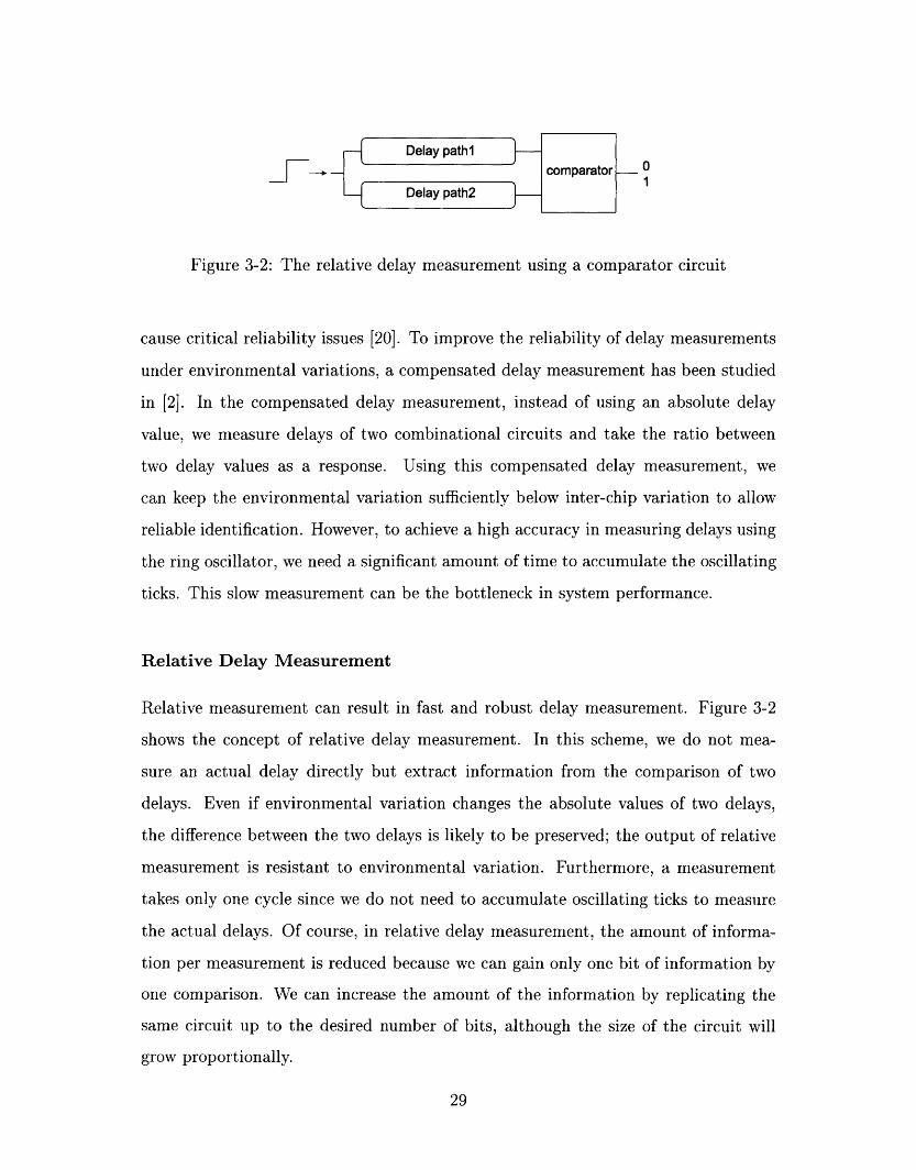
the ring oscillator, we need a significant amount of time to accumulate the oscillating
ticks. This slow measurement can be the bottleneck in system performance.
Relative Delay Measurement
Relative measurement can result in fast and robust delay measurement. Figure 3-2
shows the concept of relative delay measurement. In this scheme, we do not mea-
sure an actual delay directly but extract information from the comparison of two
delays. Even if environmental variation changes the absolute values of two delays,
the difference between the two delays is likely to be preserved; the output of relative
measurement is resistant to environmental variation. Furthermore, a measurement
takes only one cycle since we do not need to accumulate oscillating ticks to measure
the actual delays. Of course, in relative delay measurement, the amount of informa-
tion per measurement is reduced because we can gain only one bit of information by
one comparison. We can increase the amount of the information by replicating the
same circuit up to the desired number of bits, although the size of the circuit will
grow proportionally.
29
Page 30
3.1.3 Generating Challenge-Response Pairs
Assuming no environmental noise, a PUF is a deterministic function whose responses
are sensitive to delay variation in an IC. To identify individual ICs, we generate
challenge-response pairs (CRPs) for each PUF, where the challenge can be a digital (or
possibly analog) input stimulus, and the response depends on the transient behavior
of the IC. A precisely measured delay and the delay ratio of two or more delays have
been used as a PUF response in [8]. In this work, we use the digital output of a
comparator called an arbiter as the PUF response.
We build a network of logic devices. The configuration of this network is deter-
mined by the challenge vector c = (c 1, c2,...,Cm). There are two symmetric delay
paths that go through the network, and a comparator generates a one-bit response
by comparing two delays. Since the response is decided deterministically by a given
challenge, there are 2m possible CRPs for a PUF, where m is the length of a challenge
vector.
Since the PUF is designed to be highly sensitive to the process variation of delays
in ICs, the responses of the same challenge across ICs can be different from each
other. We define the inter-chip variation r between two different PUFs as
T = Prob(Ri(c) :7 Rj(c)),
where Ri(c) is the response of the ith IC on a random challenge c, and i -4 j. By
generating a sufficient number of CRPs, we can identify each IC with a negligible
probability of error.
3.2 Arbiter-Based PUF
In this section, we describe an arbiter-based PUF, which utilizes relative delay mea-
surement to generate CRPs.
30
Page 31
3.2.1 General Description
In general, an arbiter-based PUF is composed of delay paths and an arbiter at the
end of the delay paths. Figure 3-3 depicts the structure of an arbiter-based PUF.
In this scheme, we excite two delay paths simultaneously and make the transitions
race against each other. Then the arbiter at the end of the delay paths determines
which rising edge arrives first and sets its output to 0 or 1 depending on a winner.
This circuit takes an n-bit challenge (bi) as an input to configure the delay paths and
generates a one-bit response as an output.
Switch component
01
Arbiter-based PUF circuit
be ->
Switch component operation Arbiter operation
Figure 3-3: The structure of an arbiter-based PUF (basic arbiter scheme).
There are m switches and each of them can change the configuration of delay
paths. Thus, the number of possible configurations of delay paths is 2m. At the end
of the circuit, the delay difference between top and bottom paths is determined by
the configuration of delay paths, and we denote the difference by A(c). The arbiter
outputs 0 if A(c) is greater than or equal to zero. Otherwise, it outputs 1.
Process variation changes A(c) across ICs. When the amount of variation is
greater than I((c)l, the response of an arbiter can be changed. Therefore, the chal-
lenges whose IA(c)l's are less than maximum process variation can give inter-chip
variation in PUF responses. For the challenges whose IA(c)l is greater than the max-
31
-F-->
Page 32
imum process variation, responses are biased to 0 or 1 and do not change across ICs.
In order to maximize the inter-chip variation, the delay paths must be placed and
routed as symmetrically as possible so as to minimize IA(c)l.
3.2.2 Switch Blocks and Delay Paths
Figure 3-4 details the switch component of delay paths. This switch connects its two
input ports (io and ii) to the output ports (oo and ol) with different configurations
depending on the control bit (bi); for bi=O the paths go straight through, while for
bi=1 they are crossed. It is simply implemented with a pair of 2-to-1 multiplexers
and buffers.
Figure 3-4: Implementation of a switch component.
In our test-chips, we symmetrically place and route the cells and cover the entire
chip effectively using the wires in a delay circuit. This layout technique makes it
extremely difficult for an adversary to probe internal nodes to read out a logic value
without breaking the PUF, i.e., without changing the delays of wires or transistors.
If racing paths are symmetric in the layout regardless of the challenge bits and
an arbiter is not biased to either path, a a response is equally likely to be 0 or 1.
The response is determined only by the delay variation in the manufacturing of ICs.
Consequently, we wish to make delay paths as symmetric as possible to give a PUF
sufficient inter-chip variation.
32
Page 33
3.2.3 Arbiter
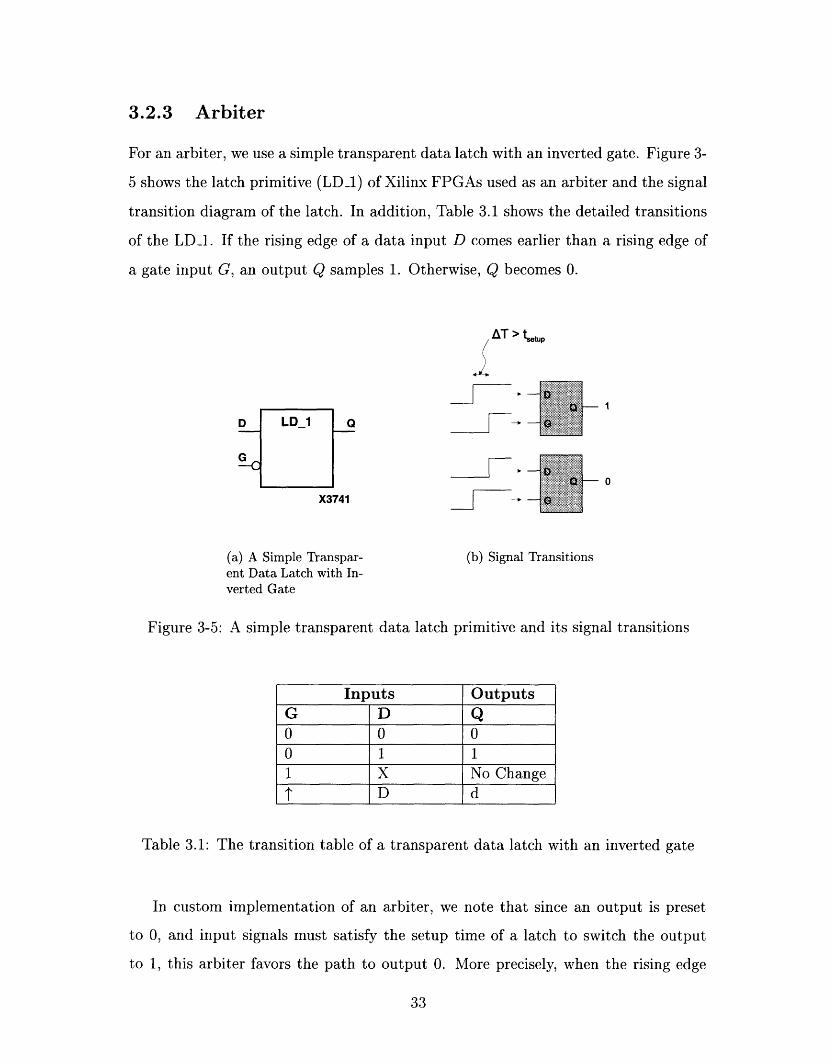
For an arbiter, we use a simple transparent data latch with an inverted gate. Figure 3-
5 shows the latch primitive (LD_1) of Xilinx FPGAs used as an arbiter and the signal
transition diagram of the latch. In addition, Table 3.1 shows the detailed transitions
of the LD_1. If the rising edge of a data input D comes earlier than a rising edge of
a gate input G, an output Q samples 1. Otherwise, Q becomes 0.
AT > t,,p
:S- i Q~~~~ __ I
I·~~ 0_ 11 E~ e o
X3741 -
(a) A Simple Transpar- (b) Signal Transitionsent Data Latch with In-verted Gate
Figure 3-5: A simple transparent data latch primitive and its signal transitions
Inputs OutputsG D QO O 00 1 11 X No Changet D d
Table 3.1: The transition table of a transparent data latch with an inverted gate
In custom implementation of an arbiter, we note that since an output is preset
to 0, and input signals must satisfy the setup time of a latch to switch the output
to 1, this arbiter favors the path to output 0. More precisely, when the rising edge
33
Page 34
of D comes earlier than that of G, an ideal arbiter output must be 1. However, if
the time difference between two signals is less than the setup time of the latch, an
output remains at 0 instead of being switched to 1. This property introduces a skew
factor to a delay model of arbiter-based PUFs. We discuss the influence of this skew
factor to inter-chip variation in Chapter 4. As a result of this skew, only 10% of total
responses are Is on average. This imbalance of PUF responses significantly reduces
the identification capability of PUFs.
We can compensate for the skews by fixing several challenge bits to effectively
lengthen the delay path connected to a gate input. Figure 3-6 shows how the com-
pensation works. Since Prob(b = 0) = Prob(b = 1) = 1, an effective skew in front
of the nth stage is s 2, where s > 0 is the skew of arbiter. When Al > A/2, we
fix b at 0, and otherwise, we fix it to 1. After fixing the nth bit, the effective skew
becomes s - Max(Al, A2), which is smaller than the original effective skew. In order
to determine whether A > \ 2 or not, a PUF is tested by 200 CRPs when b = 0,
and b = 1. If the number of Is when b = 0 is greater than when b = 1, b must be
fixed to 0. Otherwise, we fix bn to 1. Recursively, we fix the next most significant bit
until Prob(R(c) = 1) approaches 2. From experiments, we need to fix 12 of challenge
bits to achieve roughly 50% O's and 's in responses. After this compensation, the
size of a challenge vector space is reduced from 264 to 252.
b,, = 0 b,,n = 1
q S
Al= q-p A2= r-s
Figure 3-6: Compensating for the arbiter skew by fixing the most significant bits ofa challenge vector.
34
Page 35
3.3 Analysis and Characterization of Arbiter-Based
PUF
In this section, we present the primary characteristics of arbiter-based PUFs such as
inter-chip variation, measurement noise, and environmental variations, which decide
the viability of this scheme.
Inter-chip variation is the measure of a distance between CRPs from two different
PUFs. To identify each PUF from the billions of others, there must be a considerable
amount of inter-chip variation between PUFs. In Section 3.3.1, we show experimental
results of inter-chip variation between different PUFs.
Since a PUF uses an analog delay characteristic of an IC, PUF responses can be
sensitive to environmental changes such as temperature and power supply voltage
variation. Section 3.3.2 examines the causes of unreliability, such as measurement
noise, environmental variation, and an aging effect. We show the experimental results
of measurement noise and environmental variation over a practical range. In addition,
we examine an aging effect that can potentially degrade identification capability after
prolonged use.
3.3.1 Inter-chip Variation
Information-Bearing Challenges
Let information-bearing challenges be the challenges whose responses in a number of
different PUFs are not equal. We need a considerable number of information-bearing
challenges to identify each PUF. To examine the existence of information-bearing
challenges, we have measured responses for 10,000 challenges using 37 test-chips. For
each challenge, we have calculated the probability of a response being 1 as follows.
p = Pr(R(c) = 1) = ,37,
35
Page 36
Pr[Response = 1]
Figure 3-7: The density function of the random variable p = Prob(R(c) = 1)
where k is the number of PUFs that output 1. Figure 3-7 shows the density function
of the random variable p for 10,000 challenges. When p = 0 or p = 1, the challenge
does not generate any information since all PUF responses are equal. Except for the
cases when p = 0 or 1, more than 80% of the total challenges are information-bearing
challenges.
We assume that process variation and the distribution of (c), the delay difference
between the top and bottom paths, are Gaussian (cf. Chapter 4). Let ap and a be
the standard deviations of process variation and \(c), respectively. This probabilistic
model can be simulated using MATLAB. In Figure 3-7, we have evaluated the model
parameter ap = " by fitting the simulation results into the experimental results.ap
The evaluated p is around 1.5. It is significantly smaller than up ~ 25 from the
FPGA experiments in [2]. This difference comes from the asymmetry of delay paths
in FPGAs, which increase oru significantly.
36
Page 37
Definition and evaluation of inter-chip variation
Definition 3.3.1. Here, we define the inter-chip variation between two different PUFs
as below. For two different PUF responses Ri(c) and Rj(c) to a challenge c, let
D 1 Ri(c) Rj(c)
0 Ri (c) = Rj(c)
For a random challenge set C, we define the inter-chip variation Yi,j between PUF i
and j as
Yi,j = i C Di,j(c).cEC
For convenience, we denote the inter-chip variation by (100. Yi,j)%.
We have evaluated yiij's from 190 arbiter-based PUF pairs using a random chal-
lenge set C, where CI = 100, 000. In order to improve the reliability, the majority of
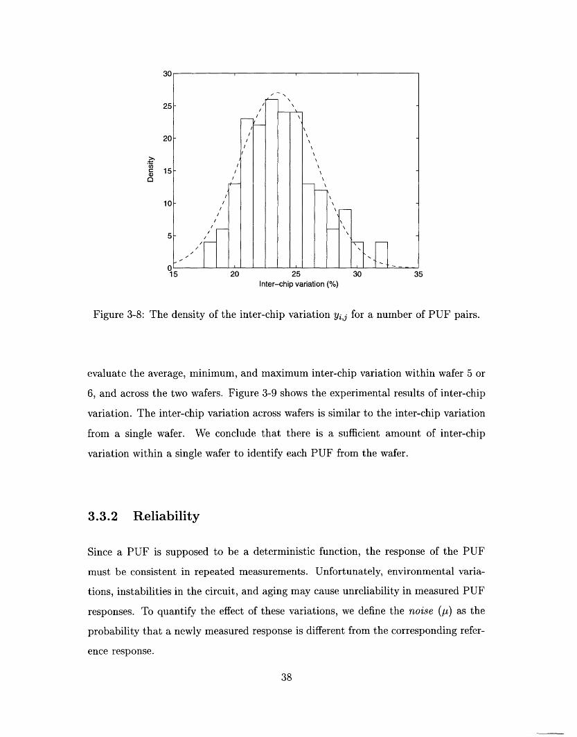
11 repeated measurements has been used as a response. Figure 3-8 shows the density
function of 190 evaluated inter-chip variations. Our test-chips have 23% inter-chip
variation on average, and the minimum inter-chip variation is 17%.
Assuming that all measurements of Di,j(c) are independent of each other, the
distribution of i,j can be approximated to Gaussian when C I is large. Generally
speaking, the shape of Figure 3-8 follows our Gaussian assumption. We present the
detailed model of inter-chip variation in Chapter 4.
Inter-chip variation across wafers
Since manufacturing variation consists of die-to-die, wafer-to-wafer, and lot-to-lot
variations, inter-chip variation can possibly be dependent on die and wafer locations.
To guarantee that there is sufficient inter-chip variation between the PUFs from the
same wafer, we must examine the inter-chip variation within a single wafer and across
wafers.
In this experiment, we use two sets of PUFs. One set corresponds to the PUFs
manufactured from wafer 5 in our TSMC run, and the other is from wafer 6. We
37
Page 38
cC
0
5Inter-chip variation (%)
Figure 3-8: The density of the inter-chip variation Yij for a number of PUF pairs.
evaluate the average, minimum, and maximum inter-chip variation within wafer 5 or
6, and across the two wafers. Figure 3-9 shows the experimental results of inter-chip
variation. The inter-chip variation across wafers is similar to the inter-chip variation
from a single wafer. We conclude that there is a sufficient amount of inter-chip
variation within a single wafer to identify each PUF from the wafer.
3.3.2 Reliability
Since a PUF is supposed to be a deterministic function, the response of the PUF
must be consistent in repeated measurements. Unfortunately, environmental varia-
tions, instabilities in the circuit, and aging may cause unreliability in measured PUF
responses. To quantify the effect of these variations, we define the noise () as the
probability that a newly measured response is different from the corresponding refer-
ence response.
38
Page 39
Figure 3-9: The inter-chip variation of the PUFs from a single wafer and across wafers.
Measurement noise
A PUF response may change due to variations within a circuit even without envi-
ronmental variation, which is called measurement noise (/Um). For some challenges, a
setup time violation for an arbiter may lead to an unreliable response. Furthermore,
junction temperatures or internal voltages may slightly fluctuate as the circuit oper-
ates This fluctuation can change the delay characteristics of PUFs. In the reference
environment, we have estimated ]um ~ 0.7%.
Environmental variations
Temperature or power supply voltage variations can significantly change circuit de-
lays and lead to unreliable responses. Since we exploit relative delay measurement,
arbiter-based PUFs are robust to such environmental variations. Figure 3-10 shows
the amount of environmental variation introduced by temperature (t) and voltage
variations (). The reference responses are measured at 27 C and 1.8V power
supply voltage. In this experiment, 10,000 challenges are used to estimate environ-
39
40
35aa(aHn0300Ma'
25
g20.5
15cm
o 10
CL 5
0
[]Min
* AverageC Max
In wafer 5 In wafer 6 Across the wafers
Page 40
Power supply voltage(V) (reference voltage = 1.8V)
j76 1.77 1.78 1.79 1.8 1.81 1.82 1.83 1.84 1.85
Max temperature variation(4.82%),4.5 4.5
° 4 _/ 4Max voltage variation( 3.74%)
Jg 3.5 X3.5
3- 3
w 2.5 C-2.5
2 2
1.5 - ~~~~co~~~~~~~~~~~~~~~~1.5a
Xz"~~~~~~~~ 2 +:SVoltage variations 1
0.5 0.50 5 10 15 20 25 30 35 40 45
Difference from reference temperature(27C) (C)
Figure 3-10: The variation of PUF responses subjected to temperature and supplyvoltage changes.
mental variations. Even if the temperature increases more than 40 degrees to 70 °C,
/t - 4.82%. Also, with ± 2% power supply voltage variation, ,u, - 3.74%. Both t
and /, are well below the inter-chip variation of 23%.
3.3.3 Performance
For a given 64-bit challenge, it takes 50 ns for an input rising edge to transmit
across the 64-stage parameterized delay circuit and evaluate an output at the arbiter.
Therefore, if we want to generate 450 CRPs to distinguish billions of arbiter-based
PUFs (cf. Section 4.4), it takes about 22.5 /us. This is sufficiently fast for most
applications since a PUF is evaluated only infrequently to obtain a secret. We can
also boost the performance by replicating multiple delay paths and arbiters to evaluate
the responses in parallel.
3.3.4 Aging
Electro-migration and hot-carrier effects cause the long-term degradation of the reli-
ability of wires and transistors in an IC [4]. Since the behavior of a PUF relies on its
40
Page 41
1.
1
CY
a)
P0a.°.
co
.c 0.5
A.
0 5 10 15 20 25days
Figure 3-11: The aging effect on an arbiter-based PUF for 25 days.
transient response, we assume that the aging could seriously affect the security and
reliability of a PUF. If the change due to aging is significant, we may not be able to
recognize a PUF after the PUF has undergone long-term usage.
While we believe that the effect of aging is not a major problem compared to en-
vironmental variation, we have run a long-term aging experiment. Figure 3-11 shows
the results of an aging test for one month. In the beginning of the test, we gener-
ated 100,000 CRPs as reference CRPs. During the test, we calculate the distance
from new CRPs to the reference CRPs. The figure shows variation in the distance.
Since the distance has not been notably increased over the 0.7% measurement noise,
we conclude that there is no significant aging effect for a one-month test in a nor-
mal operating environment. In future work, the test must be performed in extreme
environments such as high temperature and significant fluctuation of supply voltage.
41
I · · ·~~~~~~~~~~~~~~~~~~~~~~~~~~-F
7 / 'I., _ _.,_ . ;
A I F~~
Page 43
Chapter 4
Modeling an Arbiter-Based PUF
In this chapter, we introduce the delay model of an arbiter-based PUF. We have
already verified the feasibility of arbiter-based PUFs using 37 test-chips in Chapter 3.
To prove that each PUF can be identified from billions of replicates, we introduce the
probabilistic delay variation model. We estimate the parameters of the model using
experimental results. Using the estimated parameters, we prove the identification
capability of arbiter-based PUFs.
We propose a general parameter estimation method. When a model parameter z
cannot be directly estimated but can be represented as a function of other estimable
parameters, we can calculate the estimate from the estimates of other parameters.
Using the general method, we can calculate the accuracy interval of the estimate i and
the error probability of the accuracy interval from the estimates of other parameters
and their accuracy intervals.
We can verify the correctness of the delay model from an accuracy interval analysis.
If experimental results do not follow the model, then we introduce a non-linear factor
into the model and measure an amount of non-linearity in the experimental results.
This measured non-linearity can be exploited as the metric of modeling complexity
to examine the difficulty of model building in Chapter 6.
Section 4.1 presents a delay model of arbiter-based PUFs. Based on the model,
Section 4.2 gives expressions of primary model parameters. These expressions are
used to estimate the parameters as well as accuracy intervals of the parameters from
43
Page 44
experimental results. Section 4.3 shows the experimental results of parameter esti-
mation and verifies the correctness of our model with the presented theory. Section
4.4 proves the identification capability of arbiter-based PUFs based on inter-chip
variation and maximum environmental variation from experimental results.
4.1 Delay Model
For deep sub-micron technologies, a combination of device physics, die location de-
pendence, optical proximity effect, micro-loading in etching, and deposition may lead
to heterogeneous and non-monotonic relationships among the process parameters.
For the circuit that consists of continuous and differentiable functions, statistical de-
lay variation can be approximated to a linear function of process conditions [16].
Therefore, without detailed understanding of the individual contributions of process
conditions, we may assume that the propagation delay variation is Gaussian.
4.1.1 Linear Delay Model
In the description of our model, arbiter-based PUFs are numbered from 1 to n. We
denote a challenge as c. Let Ri(c) be the response of a challenge c measured in the ith
PUF. In arbiter-based PUFs, Ri(c) is decided by a sign of a delay difference between
top and bottom paths at the end of the delay paths We denote the delay difference as
Ai(c). In Section 3.2.3, we described the arbiter implementation using simple latches
and the asymmetric behavior of the arbiter by a setup time constraint of an actual
latch. This asymmetry introduces a skew in our delay model. We denote the skew of
an arbiter in the ith PUF by si. With Ai(c) and si, we model Ri(c) as follows.
R 1, if si +Ai(c) < 0,
0, if si + Ai() > 0.
In our model, we decompose Ai(c) into A(c) and pi(c),
Ai (c) = A(c) + pi(c), (4.1)
44
__
Page 45
where \(c) is a delay difference without process variation and pi(c) is a process
variation factor for a given challenge c. We can represent A(c) as
A(c)= (d, c),
where d = (do, d, ... , dm) is a constant vector and c = (co, C1, .. ,Cm), i E (--1, 1}
is a random challenge vector (cf. Section 5.2.1). When m is sufficiently large, the
distribution of A\(c) can be approximated to Gaussian by the Central Limit Theorem.
Since each vi has a zero mean,
A(c) N(O, v<),
where oa = ldII. We assume the process variation pi(c) to be Gaussian,
pi(c) ~ N(O, p).
Hence,
Ai (c) N(O, v),
where a = / + . In this model, (c) and pi(c) are assumed to be independent
of each other.
4.1.2 Non-Linear Delay Model
Ideally, statistical behavior of PUF responses must follow the linear delay model (cf.
Section 5.2.1). However, in real circuits, various kinds of noise such as measurement
noise, cross-coupling between wires, and environmental variations cause the delay
model to be non-linear. In order to consider these non-linear effects, we extend the
original model to
hi (c) = A(c) + pi(c) + y, (4.2)
45
Page 46
where y is a non-linearity factor. We assume that y is from an arbitrary distribution
and
17H < R, (4.3)
where R is the upper-bound of non-linearity.
To measure the non-linearity of experimental results, first, we estimate a model
parameter based on a linear delay model. If experimental results follow the linear
model, the model parameter must be estimated consistently within a high probability
accuracy interval in repeated independent experiments. Otherwise, we must introduce
non-linearity y > 0 to give an extra margin to the accuracy interval. We increase the
upper-bound R of non-linearity until all the estimates are included in the enlarged
accuracy interval. This upper-bound R represents the amount of non-linearity in the
experimental results.
4.2 Estimation of Model Parameters
In Section 4.2.1, we show how to estimate individual skews si's using a linear delay
model. In Section 4.2.2, we estimate Up = aA/ap based on the estimated skews.
In both sections, we derive the accuracy interval of an estimate and evaluate the
probability that a model parameter exists in the accuracy interval. We show how
to verify the correctness of model from accuracy intervals of estimates in repeated
independent experiments. In Section 4.2.3, we estimate ap using the extended model
with a non-linearity factor and derive an accuracy interval from the extended model.
4.2.1 Estimation of sil/a
In this section, a PUF i is fixed. Since
Si + Ai() N(Si, ),
46
-
Page 47
we obtain
Pi = Prob(Ri(c) = 1) = Prob( <oa
where
s- -si/Y e-t 2/2_ s) =f-si/ dt
o- -o X/ -7
rx et2/2Q(x) = o dt.
.co , fi
Let C be a random challenge set. From the response set of C, we define yi such
that
(4.4)1
Yi -C ZRi(c).cI C
By the law of large numbers, the binomial distribution which defines yi tends to
Yi N(pi, pi(1 - pi)/C )
(notice that pi(l - Pi) < 1/4). This proves that, when CI is sufficiently large,
Prob(lyi - pi I > ) = 2Q(-E/V/pi(l- pi)/ICI)
< 2Q(-2E J/C) (4.5)
(see the inequality (B.1) in Appendix B). From the inequality (B.4) in Appendix B
we obtain
Prob(lQ-l(yi) - Q- 1(pi)j > 6) < Prob(lYi - Pil > E), (4.6)
(4.7)
From the inequalities (4.5) and (4.6), we can prove that Prob(lyi - il > ) has the
upper bound 2Q(-2e /v).
E), f (i + )}.
47
wherel
6 = v\/ EeQ- l( i +) 2 /2
1We define f(y + ) = max{f(y -
Page 48
Given ICI measurements, we choose £ as large as possible such that the bound
2Q(-2Ev/CI) is sufficiently small, say p,. We compute 6 from Eqn. (4.7) and then,
with an error probability less than p, the skew -si/a, that is equal to Q-l(pi), exists
within the accuracy interval [Q 1-(yi) - 6, Q- 1 (yi) + 6].
4.2.2 Estimation of an/ap
In this section, we use PUF i and PUF j (i j) to evaluate the probability that
both PUFs output the same response 1. From our model, the process variation pi(c)
is from the normal distribution N(O, up). Let
Up = aA/Up
be the ratio between the standard deviation of A(c) and the standard deviation of
process variation. We can derive Prob(Rj(c) = 1, Ri(c) = 1) using the parameters
-si/a, -sjl, and Up.
Pi,j = Prob(Rj(c) = 1,Ri(c) = 1)
= Prob(sj + A(c) + pj(c) < O, si + A\(c) + pi(c) < 0)
= Prob P(c) < sj + 2 _ L<(c) pi(C) S< i 2 (c)
Q(j/) 1 +-ta p)Q(-(Si/U) 1 + - t) dt
P(-Sip/, -Sj /, ap),
where
P(v,w,z) = j| e + Q( 1+ z - tz)Q(w 1 +z - tz) dt
is a continuous differentiable function of three variables. For fixed i and j, v = -si/a
and w = -sjla are fixed. Intuitively, P(v, w, z) is a monotonically increasing function
in z since a larger z = Up means less process variation and two responses are more
48
Page 49
likely to be equal if there is less process variation. Thus, we can use a simple binary
search to evaluate
z = P(v, w, a) (4.8)
as a solution of the equation 0 = P(v, w, z).
Let
(C) 1 Ri(c)= 1,Rj(c)= 1
0 otherwise
where i L j. For a random challenge set C, we define yij as
Yi,j = C Ce Dij( (49)
Similarly, by the law of large numbers, the binomial distribution which defines Yi,j
tends to
Yi,j - N(P i,j(l -pj)/C)
(notice that pi,j(l - pi,j) < 1/4). This proves that, when ICI is sufficiently large 2,
Prob(lyi,j - pi,jl > ) = 2Q(-/El/i,j(1 -pi,j)/C[)
< 2Q(-2E 1/j) (4.10)
In Appendix A, we provide a general method to estimate a hidden parameter in
a general model from the estimates of known parameters. If the hidden parameter
can be represented as the function of directly estimable parameters, we can calculate
the accuracy interval of the hidden parameter from the accuracy intervals of other
parameters. The probability that the hidden model parameter exists in the accuracy
interval can also be evaluated using the general method.
In our model, Up is the hidden parameter and it can be represented as a function
of -sil/, -sj/a, and Pij in Eqn. (4.8). Since we can directly estimate -sie, -sj/r,
2 Do not confuse E with the one used in Section 4.2.1.
49
Page 50
and Pij, we can estimate Up and its accuracy interval using the general method.
We denote model parameters by v, w, 0, and z. Each notation means
V -- Si/,
W = -- Sjl
0 = Pij,
Z = Up.
We can directly estimate v,w, and 0 from experimental results yi, Yj and Yij as follows.
= Q-'(Yi)
W = Q-1 (yj),
0= Yi,j
Using the estimates v, , and 0, we can calculate the estimate of z as
z = P(v, b, ). (4.11)
We denote estimation errors v - v, tb - w, 0 - 0, and 2 - z by Av, Aw, AO, and Az,
respectively.
We assume that each parameter has an accuracy interval with an upper-bounded
error probability. If we denote the error probabilities by Pv, Pw, and Po, then
Pv > Prob(lAvl = I -vl > e,), (4.12)
Pw > Prob(JAw = Ib-wl > w),
po > Prob(IAOI = 10 - > o).
We assume that v,w, and s are sufficiently small.
50
Page 51
Using partial derivatives, can be approximated to
z = P(V, , )
= P(v +Av,w+ Aw, + A)
Pw,) + v P(v, w, ) +19V
Aw-ow
We derive the upper-bound of IAzl as follows.
IjZI = - l= = - P - (v,w, )l
- Ava P(v, w, 0) + Awa P (v, , )av aw
< vl.
P(v, w, 9)
+ AoaaoI P(v,w,) +lawl wa P
< vli aP(V W ) + W Ia P av aw
a+ AO9P'(v, w, 9).09
P(V, )
+ L9l1 IoP(v,w, )
v, W, ) I + Ee P (v, W, ) .ao
The first inequality holds by the triangle inequality. The second inequality holds when
estimation errors lav, lIwl, and AOl are less than the width of accuracy intervals
Ev, w, and Co, respectively. From Eqn. (4.12), these inequalities hold with at least
(1 - pv)(1 - pw)(1 - Po) probability.
If we define E, as
O)l + EoaP -(v, w, ) ,
then we can formulate the accuracy interval and its probability of the model parameter
z by
Prob(Iz - I < E,) > (1 - pv)(l - pw)(l - po) = 1 - Pz, (4.13)
where Pz is defined as the upper-bound of the error probability of the accuracy interval.
Assuming that E, w, Co are sufficiently small, we approximate E, to
Ez c_ £Ea P(',, )I+E ±W PI-p_(oi, , )J +E P-P(V, &, )lJ.vl aw .o (4.14)
51
E, -_ EI a P + (V , ) I + E IaPt(V, ,av aw
Page 52
C)
EC)
a,-
:00
Accuracy interval with error probability p
region
1 2 3 4
Number of experiments
Figure 4-1: Accuracy intervals and their overlapping region.
Thus, we can calculate E, of the parameter z from E, , AE, and partial derivatives.
The error probability of the accuracy interval can be evaluated from Pv, Pw, and po
using Eqn. (4.13).
The existence of an overlap region in repeated independent experiments
From n repeated independent experiments, we can plot the estimates of a model
parameter and their accuracy intervals. Figure 4-1 shows the figure of accuracy
intervals. In this figure, the x-axis denotes an experiment number and the y-axis
means the value of the model parameter. For each experiment, we draw an accuracy
interval parallel to y-axis.
From the figure, we can check the existence of an overlapping region of all n
accuracy intervals. Let Pi be the upper-bound of an error probability of an accuracy
interval i. If the model is correct, then the probability of existence of the overlap
region among n accuracy intervals is TJini= (1-pi) since all experiments are independent
of each other.
The correctness of model assumptions can be verified from existence of this over-
lapping region. In our model, we assumed that delays are additive. The distributions
52
_ -
Page 53
of Ai(c) and pi(c) are independent of each other as well as Gaussian. Let po be the
probability of existence of an overlap region. If an overlap does not exist when po
is close to 1, we conclude that the experimental results do not follow the model as-
sumptions. Thus, we must extend the model to consider unknown non-linearity . We
measure an amount of non-linearity using the suggested model in Section 4.1.2.
4.2.3 Estimation of uaz/cp using a Non-linear Delay Model
In this section, we re-calculate the accuracy intervals of ap estimates using the non-
linear delay model. Intuitively, adding a non-linearity factor to a linear delay model
will give an extra margin to the accuracy interval.
Similar to Section 4.2.2, we formulate the probability Prob(Rj(c) = 1, Ri(c) = 1)
considering the non-linearity factor y.
Pi,j = Prob(Rj(c) = 1,Ri(c) = 1)
= Prob(sj + A(c) + pj(c) + a < O, si + A(c) + pi(c) + y < O)
= Prob (pj(c) < Aj, p(c) < Ai) . (4.15)
where
s i n 7 (c)Ai = - U -ff ..2 ap - Y
We define a normalized non-linearity factor as
I = y/5p.
Then, from Eqn. (4.3),
-R' < ' < R',
53
Page 54
where R' = R/ap. Using -ai/a, -aj/a, Up, and y', we derive Pi,j as follows.
Pij =
-oo
e- t2 /2
Q(-(s,/u) (1 + c4 - tap - ?')Q(-(s/i/) 1 + 2 - tcrp - ?y') dtv 27r
= P2 (-i/o, -j/o, aoP, '),
where
f=Q(-o v - tz -t-o 00V--7
P2(V, W, , r) = r)Q(w 1+ z 2
As solutions of 0 = P2 (v, w, z, r),
z = P(v,w,0,r).
Similar to Section 4.2.2, we can use a simple binary search to evaluate P2(v, w, 0, r)
when v,w,O, and r are given.
We use the same notations v, w, 0, and z for the model parameters -si/a, -sj/a,
Pi,j, and Up. We add r, which means the normalized non-linearity ?y', to the model.
From the definition of y,
Pr = Prob(lrl > R') = 0.
Assuming that R' is sufficiently small, we derive the accuracy interval width ez similar
to Section 4.2.2 as follows.
£z £P2 aw
+Ea I a P2- 0) +R MIa P Pvtb,6O)1. (4.16)+010 P, , 0) R'P ,b,,)I.
Compared to Eqn. (4.14), the non-linearity term R'9P (, h,,0) has been
added to give an extra margin to the accuracy interval. Since Pr = 0, the error
probability of the accuracy interval does not change.
54
- tz - r) dt
Page 55
-0.12
-0.14
0
'_ -0.1
-0.1
-0.2.
-0.1Overlap RegionOverlap Region
0
In
'-I
-0.26 I0 1 0 20 30 40 50
Number of experiments
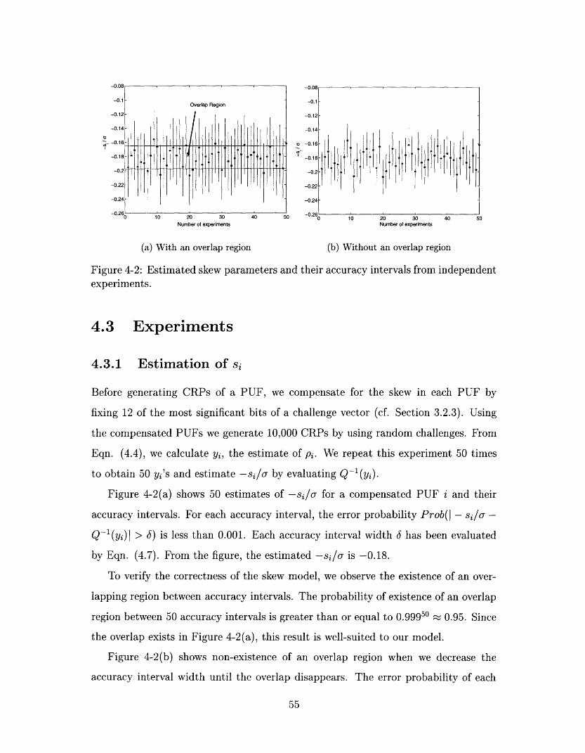
(a) With an overlap region (b) Without an overlap region
Figure 4-2: Estimated skew parameters and their accuracy intervals from independentexperiments.
4.3 Experiments
4.3.1 Estimation of si
Before generating CRPs of a PUF, we compensate for the skew in each PUF by
fixing 12 of the most significant bits of a challenge vector (cf. Section 3.2.3). Using
the compensated PUFs we generate 10,000 CRPs by using random challenges. From
Eqn. (4.4), we calculate yi, the estimate of Pi. We repeat this experiment 50 times
to obtain 50 yi's and estimate -si/a by evaluating Q- 1 (yi).
Figure 4-2(a) shows 50 estimates of -si/cT for a compensated PUF i and their
accuracy intervals. For each accuracy interval, the error probability Prob(l - si/a -
Q-(yi)l > ) is less than 0.001. Each accuracy interval width 6 has been evaluated
by Eqn. (4.7). From the figure, the estimated -si/a is -0.18.
To verify the correctness of the skew model, we observe the existence of an over-
lapping region between accuracy intervals. The probability of existence of an overlap
region between 50 accuracy intervals is greater than or equal to 0.99950 0.95. Since
the overlap exists in Figure 4-2(a), this result is well-suited to our model.
Figure 4-2(b) shows non-existence of an overlap region when we decrease the
accuracy interval width until the overlap disappears. The error probability of each
55
I I
I. I
. , I i
I. I · , *
l , I I I I I
I i I I , 1 1l
l .
' I l I
-U.Z4 I I' [.... II I I
I
Page 56
O
2.4No overlapping region
2.2
2
12 J I1
1.20 2 4 6 8 10
Number of experiments Number of experiments
(a) With an overlap region (b) Without an overlap region
Figure 4-3: Estimated up and their accuracy intervals from independent experiments.
accuracy interval is 5.74%. Since the probability of existence of an overlap po is only
0.942650 = 0.052, This result does not contradict our model. Thus, we conclude
that a skew in each PUF can be estimated consistently using the linear delay model.
The estimate and accuracy interval of a skew can be used in estimating other model
parameters.
4.3.2 Estimation of ua/up
To estimate up, we use 10 independent pairs of two different PUFs. For each pair,
we generate 20,000 CRPs and calculate yi and yj to estimate the skews of two PUFs.
Using Eqn. (4.9), we estimate pi,j by evaluating Yi,j. These three estimates i, j,
and Yi,j are used to to estimate up.
Figure 4-3(a) shows the estimates of ap and their accuracy intervals in 10 repeated
experiments. These experiments are independent of each other. The estimates of up
have been calculated by Eqn. (4.11) and their accuracy intervals have been evaluated
by Eqn. (4.14). In this figure, the error probability of each accuracy interval is 0.3497.
The estimated up is around 1.75, which means that aA is only 1.75 times larger than
the process variation up.
56
I I I . I
Page 57
We can verify the existence of overlap region L = [1.68,1.83] from the figure.
Since 10 independent experiments were performed, the probability of the existence
of an overlap region is 1.35%. The existence of this overlap means that experimental
results are well-suited to our model. In other words, the estimates of repeated exper-
iments are sufficiently consistent, and therefore, we can obtain the accurate estimate
of up. We do not need to introduce non-linearity to give an extra margin to accuracy
intervals.
To verify our model, we decrease the accuracy interval widths until the overlap
does not exist. Figure 4-3(b) shows the non-existence of the overlap when the error
probability of each accuracy interval is 68.65%. In this case, p, is only 7.5 10-6.
Since p, is extremely small, the experimental results do not contradict our model.
4.3.3 Estimation of Non-linearity
We estimate non-linearity in experimental results using the non-linear delay model
in Section 4.1.2. Assuming that y = 0, we estimate a model parameter based on
the original linear delay model. We denote Pt as the error probability of an accuracy
interval when there is no overlap between accuracy intervals of estimates. Then, we
introduce the non-linearity y > 0 to the model and increase the maximum value of
normalized non-linearity R' until we gain the overlap. The increase of R' enlarge the
width of accuracy interval following the definition of Eqn. (4.16). We denote R as
the minimum required non-linearity to gain the overlap region.
To prove our non-linear delay model, we have tested the non-linearity of PUF
responses from the simulation of two different arbiter-based PUF models. The first
model is an additive delay model without non-linear noise. We assume that every
delay segment in an arbiter circuit is a constant and the process variation in each
delay component is Gaussian. From the additive delay model in Section 5.2.1, we
model the delay difference between top and bottom paths as the inner product of the
random challenge vector c and the constant delay vector di. The delay vector di is
composed of a common delay vector d and process variation vector pi. The common
delay vector d consists of the delay values of circuit components without considering
57
Page 58
process variation. Each component of a process variation vector Pi is a zero-mean
Gaussian. We set p, which can be represented as is1il (cf. Section 4.4), to two.
There is no arbiter skew and measurement noise in this model.
The second model is an additive delay model with non-linear noise. The noise
source N is added at the end of delay paths to introduce non-linear random noise to
the model. As an example of non-linear random noise, we use random numbers from
x 2 -distribution. For X - X2(v, 1), where v = 20, we define N as
X-vN = 3 , where v = 20.3v
The mean and standard deviation of N are a zero and aA/10, respectively. This
model does not have an arbiter skew and up = 2.
10-°.3 10- .
10-°,'
Pt
Figure 4-4: Comparison of pt-R' curves depending on the existence of non-linear noise.
Figure 4-4 shows the Pt - Rt curves from simulated responses of the first and
second models. Since the two models have the same amount of process variation up,
we can directly compare the non-linearity R', which is normalized with up. From
the figure, the first model requires more non-linearity than the second model to fit
the experimental results to the linear delay model. This result follows the fact that
the second model has more non-linear random noise that cannot be predicted by
58
Page 59
a linear algorithm than the first model. When an adversary is willing to build a
software model to predict responses, the second model is more difficult to break than
the first model since the random noise causes prediction errors. Thus, the measured
non-linearity from this method is related to the modeling complexity of arbiter-based
PUFs. We exploit this method to analyze the security of alternative types of PUFs
in Chapter 6.
4.4 Identification/Authentication Capability
We study the identification/authentication capability of arbiter-based PUFs based
on inter-chip variation T and noise probability ,u. Since environmental variation is
the primary factor of noise, we consider only environmental variation for noise in this
section. We represent the identification/authentication capability by the probability
of errors that can occur in identifying/authenticating billions of PUFs. In the calcu-
lation of the error probability, we assume that CRP measurements are independent
of each other. Since T and are related to the number of PUF delay stages m, we
calculate appropriate m to gain the desired T and u using our delay model.
4.4.1 Inter-chip Variation and Environmental Variation
We study how inter-chip variation and environmental variation are related to the
number of delay stages. Based on the delay model in this Chapter, we represent
and p as the function of m. When m is sufficiently large, the skew of an arbiter does
not affect PUF responses. Using the model, we evaluate the inter-chip variation and
environmental variation without the arbiter skew.
Information-bearing challenges
We can estimate the number of information-bearing challenges in the complete set
of challenges using a linear model of an arbiter-based PUF. Let k be the number of
arbiter-based PUFs. We denote the probability of a random challenge c being an
information-bearing challenge by A1. We do not consider skew in the arbiter. Using
59
Page 60
The number of PUFs (p = 1.75)
Up (the number of PUFs = 37)
Figure 4-5: The change of according to the number of PUFs and up.
Up, we can derive 77 as follows.
= I - Prob(Ri(c) = 1 for all 1 < i < k) - Prob(Ri(c) = 0 for all 1 < i < k)
00 et2/2 rtap e-v2/2 eot2 /2 roo -v2/2
= the es ( - dv)kdt- (J dv)kdt. (4.17)
Using the estimate of ap (a 1.75) in Section 4.3.2, we can calculate the number
of information-bearing challenges. From Eqn. (4.17), when k = 37, r = 0.8204.
This means that 82.04% of total challenges are information-bearing challenges. In
Section 3.3.1, we verified that around 80% of total challenges are information-bearing
challenges in our 37 test-chips, which is similar to the computed 7. We conclude that
the number of information-bearing challenges can be calculated from Eqn. (4.17).
Figure 4-5 shows the change of r according to the number of PUFs and ap. When
there are more than 1,000 of PUFs, the portion of information-bearing challenges
converges to 93%. To obtain more information-bearing challenges, we must place and
route delay components symmetrically to reduce Up.
60
-
Page 61
Inter-chip variation
The inter-chip variation r between two different PUFs is defined as
T = Prob(Ri(c) Rj(c)),
where i Z j and c is a random challenge. We can evaluate T using given model
parameters -sila, -sj/la, and up as follows.
T = T(-sij/, -sjla, up), (4.18)
where
T(v, w, z) = - -/_7 ((1 - Q(v 1 + z 2 - tz))Q(w1
+ Q(vv1 - tz)(1 - Q(wv1+ z - tz))) dt.
k z 2 - tz)
We represent r as the function of m, which is the number of delay stages. Let
pij(c) be the process variation in the jth stage of PUF i. By the Gaussian assumption
of process variation,
Pij (c) N(O , p,).
We assume that Up, is constant for every stage. Since delays are additive, we model
m
pi(c) = Pij(c).j=1
Since pij(c)'s are independent of each other,
up = /p/,.
We represented A(c), which is the delay difference between top and bottom paths
without process variation, as (d, c), where d = (d, d2 ,..., dm) is a constant vector
and c = (Cl, c2,.. ., Cm) is a random challenge vector for ci e (-1, 1}. Assuming that
61
Page 62
m is sufficiently large, we can model
a(c) N(0, o),
by the Central Limit Theorem. We denote ao, as the standard deviation of ci. Since
ci E {-1, 1} and a uniform random variable, oc, = 1. We represent aa using d as
follows.
m ~ m
UA d= Ed2 d = I Ildll.i=1 i=1
Assuming that every delay stage is identical, we can approximate
UA C
Since both cp and ua are proportional to /V, a = ± p, which is the delay
difference between top and bottom paths with process variation, is also proportional
to +'
From Eqn. (4.18), can be represented as the function of -si/a, -sj/a, and
Up. Let Si be the skew -silo when m = 64 for PUF i. We can estimate Si from
experiments (cf. Section 4.3.1). Since a is proportional to vI, we represent the skew
-si/a as a function of m as follow:
85i
Since both ai and up are proportional to /, o-p = aA/ap is a constant to m. We
conclude that8s 8j
T(m) = T( 8q. ,up),
where Si and Sj are estimated skews from PUF i and j, respectively.
Figure 4-6 shows the curve of inter-chip variation r as a function of m. For two
different PUFs, we estimate the skews Si and Sj and up (cf. Section 4.3). Based
62
Page 63
0.26
0.25
0.24
0.23
0.22
0.21
v.~0 100 200 300 400 500 600 700 800 900 1000
Number of Stages m
Figure 4-6: The change of T according to the number of the stages in delay paths.
on these parameters, we calculate T when m varies from 32 to 1024. Intuitively, the
inter-chip variation T decreases according to the increase of m because the influence of
the skews decreases while up remains constant. From the curve, T converges to 0.22,
which is the inter-chip variation of arbiter-based PUFs that have no arbiter skew.
Environmental variation
While we cannot find any appropriate model to represent the noise of PUF responses
as a function of m, we can roughly examine the relationship between the noise and
the number of stages m. At first, we consider measurement noise of arbiter-based
PUFs. Section 3.3 shows that the setup time (t,,u) of an arbiter causes measurement
noise. When i(c) is less than t,,, the arbiter is in a meta-stable state and the
response of the arbiter is unreliable. Thus, measurement noise lm is proportional to
Probli(c) < t,,u).
In our model, Ai(c) . N(si, r). When m is sufficiently large, we can approximate
Si 0.
l cm C Prob(lx < tu), where x N(0, U).
We already verified that a is proportional to Vm/. When we increase m, lm, decreases
63
i
I I
Page 64
because the increase of u reduces Prob(lxl < t,,). Table 4.1 shows experimental
results. We used FPGAs to change m in the PUF circuit. From the table, we can
verify that the measurement noise decreases according to the increase of m.
The number of stages (m) Measurement noise(%)32 0.10664 0.08696 0.078
128 0.074
Table 4.1: Measurement noises in the different number of stages.
Similarly, we can expect that environmental variation decreases according to the
increase of m. Let's assume that environmental variation on PUF circuits increases
of decreases Ai(c) by 6(c). If we denote ten as the maximum value of [6(c)l, envi-
ronmental variation p/ is proportional to Prob(lAi(c) I< ten). Therefore, using the
same arguments in the measurement noise analysis, we can conclude that the increase
of m decreases . The maximum environmental variation 4.84% from experimental
results (cf. Section 3.3) can be decreased by increasing the number of stages. We use
p = 0.0484 as the worst case environmental variation in the calculation of identifica-
tion/authentication capability in the next section.
4.4.2 Identification/Authentication Capability
Given the inter-chip variation T and environmental variation /t, we can evaluate the
identification/authentication capability of arbiter-based PUFs. We represent this
capability as the probability of errors that can occur in identifying/authenticating
billions of PUFs. Since the error probability can be reduced by using a larger number
of CRPs, we calculate the number of CRPs to make the error probability sufficiently
small (< 10-9).
For convenience, we define two probabilities, pd(t, k) and pn(t, k). When inter-
chip variation is , the probability that at least t out of k reference responses differ
64
Page 65
between two different chips is equal to
pd(t, k) = 1 - (')Ti(1 - T)k (4.19)i=--
For a single chip, when environmental variation is , the probability that at most t
out of k responses differ from the corresponding reference responses is
k
pn(t, k) = 1 I ()i (I kj. (4.20)j=t+l
Identification
When we use PUFs for the identification of registered users, there exists the server
that stores CRP profiles of N registered PUFs in its database. Each CRP profile has
k CRPs. When a user presents a PUF to the server, the server generates CRPs using
the presented PUF and compares it with all CRP profiles of the registered users in
the database. The server identifies the user by finding the minimum distance CRP
profile from the generated CRPs of the presented PUF.
In this scheme, the probability of error is equal to
k-1 I
Pe = 1 - - () Ii(1 - -)k-i(Pd(i + 1, k))N+l, (4.21)
where Pd(i, k) is the probability defined in Eqn. (4.19). We use T = 0.22 and pu = 0.048
from experimental results (cf. Section 3.3). When N = 109, we need k > 450 to
achieve Pe < 10- 9 .
This result shows that we can identify 109 PUFs with only 450 CRPs. The er-
ror probability in this identification is less than 10- 9. However, this scheme is not
practical because the comparison with all CRPs in database imposes a significant per-
formance overhead. Furthermore, we cannot distinguish a non-registered PUF since
we always choose the minimum distance profile in the database.
65
Page 66
Authentication
To avoid the comparison with all CRP profiles in database, the server first asks the
user-name of the presented key-card and authenticates the PUF in the key-card by
profile matching. This scheme is significantly faster than simple identification because
the server needs to perform profile matching only once.
In the authentication of a PUF, the server compares the CRPs of a presented PUF
with the CRP profile of a presented user-name in database. If the distance between
two CRP profiles is less than or equal to the threshold t, the server authenticate the
PUF. Otherwise, this access is rejected by the server.
In this scheme, two kinds of errors are possible.
Robustness: A user presents a valid PUF, but a server recognizes it as a wrong
PUF. The probability of this error P' is equal to
k
=pe- (k) i( 1 - )k-i = 1-b(t).i=t+1
We can see that P' decreases monotonically when t increases.
Security: When an adversary issues a wrong PUF to a server, the server authenti-
cates it by mistake. The probability of this error is
t k
"=E ()i(1 -T)k - i
i=O
Clearly, p" increases monotonically when t increases.
In n uses of authentication, we assume that an adversary tries to deceive a key-card
server by issuing a wrong PUF d times. We denote a = d/n as the frequency of
the deceiving trials. The system error probability Pe can be represented using a as
follows.
Pe = (1 - )p' + (Pe.1 (4.22)
66
Page 67
Assuming a = 0.5, our goal is to achieve Pe < 10 - 9 using a minimum k and
an appropriate t. Similar to identification, we use r = 0.22 and t = 0.048. From
calculation, Pe = 9.3 10-10 < 10- 9 when k = 443 and t = 48. We conclude that using
less than 450 CRPs we can authenticate the PUF with negligible error probability.
67
Page 69
Chapter 5
Breaking an Arbiter-Based PUF
Since an arbiter-based PUF exploits inevitable process variation in the manufacturing
of ICs, the PUF cannot be duplicated by an adversary even with the detailed knowl-
edge of a circuit. However, attacks to break arbiter-based PUFs are still possible. For
example, an adversary can build a timing accurate model to simulate the PUF cir-
cuit. Moreover, if there exists notable correlation between challenges and responses,
then an adversary can build a software model of the PUF and use it as a "virtual
counterfeit". The security of physical random functions is based on the difficulty of
response prediction (cf. Chapter 2). Therefore, these types of modeling attacks can
be critical threats to the security of arbiter-based PUFs.
In Section 5.1, we provide possible invasive and non-invasive attack models on
arbiter-based PUFs. Among the possible attack models, we provide the software
model building attack based on a machine learning algorithm called Support Vector
Machine in Section 5.2. We show how to train the algorithm using a polynomial
number of CRPs and verify the prediction accuracy of the trained algorithm using
FPGAs and custom silicon in Section 5.3.
5.1 Attack Models
In this section, we introduce possible attack models on arbiter-based PUFs. Most
of the attacks were already introduced in [2] based on the PUF that uses a MAX
69
Page 70
circuit instead of an arbiter. Though we use a different type of a PUF, an adversary
can use the same attacks since both arbiter-based PUFs and MAX-based PUFs use
the same delay path structure.
5.1.1 Duplication
If an adversary can fabricate a "counterfeit" PUF, which is logically identical with
the original PUF, he can break the authentication methodology. The term "logically
identical" means that a counterfeit PUF produces almost the same responses as the
original PUF for most of random challenges. A special case of this attack occurs when
an IC manufacturer attempts to produce two identical ICs from scratch.
Given the statistical variation inherent in manufacturing process we used, we argue
that it is impossible to produce an IC precisely enough to control the PUF that the
IC embodies. When producing two ICs in identical conditions (same production line,
same position on wafer, etc.), the manufacturing variations are still sufficient to yield
two significantly different PUFs. We have tested the PUFs from the same wafer and
verified that inter-chip variation is sufficient to identify each PUF in Section 3.3.
Following the identification capability discussion in Section 4.4, the probability
that two different PUFs are indistinguishable from each other is extremely low. Thus,
an adversary must fabricate a huge number of ICs and make comprehensive measure-
ments on each one in order to discover a match. This is a very expensive proposition,
both from economical and computational standpoint.
5.1.2 Timing-Accurate Model Building
Today, the accuracy of measurement devices is getting more precise. Though process
variation in the manufacturing of ICs is beyond the control of a manufacturer, by
measuring delays of all circuit components, an adversary can create a time-accurate
model of an original PUF and simulate the model to predict the responses of randomly
given challenges. The success of this timing-accurate model depends on the accuracy
of the measurement devices.
70
Page 71
Direct Measurement
The development of reverse engineering techniques has made it possible to extract the
important circuit information such as circuit topology and a physical dimension of
each component (cf. Chapter 1). It is also possible to directly measure the delays of
circuit components by micro-probing. These measured delays can be used to construct
a sophisticated timing model.
In order for this delay measurement to be at the level of the accuracy required
to break authentication, an adversary must remove the package of an IC and insert
probes. Alternatively, he can use non-invasive attacks such as differential power
analysis [12] and electromagnetic analysis [17] to extract information about collections
of devices. However, probing with sufficient precision is significantly difficult because
the delay of the probing device will change the measured delays. Interactions between
the probe and the circuit can introduce noise in the measurement. Moreover, in order
to insert his probes, the adversary may damage overlaid wires. Because of the high
capacitive coupling between neighboring wires (cf. [6] for the importance of capacitive
coupling between wires), damage to these overlaid wires could change the delays that
are being measured. To make the direct measurement more difficult, the circuit can
be protected by a tamper-sensing environment. How best to layout the PUF circuit
to make it highly sensitive to invasive attacks is a direction for future research.
Exhaustive Model
Clearly, a model can be built by exhaustively enumerating all possible challenges.
However, exhaustive modeling is intractable since there are an exponential number
of possible challenges. In our test-chip, a challenge is 64 bits and it takes 50 ns for
one measurement. By simple calculation, it takes more than 30,000 years to generate
all CRPs.
71
Page 72
5.1.3 Software Model Building Attacks
Non-invasive model building attacks are also possible. First, an adversary can use a
publicly available mask description of IC/PUF to build a timing-accurate model with
a polynomial number of parameters. In other words, an adversary can formulate
the responses of a PUF as a function of challenges and circuit parameters. If the
challenge-response model of the PUF circuit is linear, then an adversary can apply
a polynomial number of random challenges and monitor the responses to estimate
circuit parameters in the linear model. If the model can predict the response of the
circuit with the error probability lower than the maximum environmental variation,
the adversary can impersonate the original PUF with the model. We note that if the
PUF has been calibrated in different environments (e.g., different temperatures), the
adversary's job can be made harder.
In Section 3.3, we provided data on environmental variation and inter-chip varia-
tion of arbiter-based PUFs. When considering the model building attacks, we must
calculate the probability of being deceived by possible software models from the pre-
diction error probabilities of the models.
5.2 Software Modeling Building Attack: Support
Vector Machines
We model a PUF circuit using an additive delay model. In this model, we assume
that the delay of a path through the circuit is the sum of the delays of elementary
components. Knowing all the elementary component delays, an adversary can predict
responses for any challenge by calculating the circuit delay. The adversary's task is to
estimate the elementary delay parameters. Assuming that direct measurement of the
delays is impractical, the adversary can infer those delays from a polynomial number
of CRPs using the machine learning algorithm named Support Vector Machine.
72
Page 73
Figure 5-1: The notations of delay segments in each stage.
5.2.1 Additive Delay Model of a PUF Circuit
We denote 6 tOp(n) as a signal delay from the starting point to the top path at the end
of the nth stage. Similarly, bottom (n) denotes the delay of the bottom path.
Figure 5-1 shows the notations of the delay segments Pn, qn,, r, and Sn in each stage.
We can derive top(i + 1) as a function of 6top(i - 1), bottom(i- 1), and the delay
segments of the ith stage as follows.
Jtop(i + 1)
6bottom (i + 1)
2 (Pi+l + 6top(i)) +
+ - i+1 (Si+l + 6bottom(i))2
- i+ (qi+l + 6bottom(i)) +
+ - Ci+' (ri+l + 6top(i)),
(5.1)
where Ci E {-1, 1} is a challenge bit of the ith stage.
Then, we denote AZ(n) as the difference between tp(n) and bottom(n). By sub-
73
(5.2)
Page 74
tracting Eqn. (5.2) from Eqn. (5.1), we can derive
A(i + 1) = Ci+1 (i) + ai+lCi+l + Pi+1,
where
a n =Pn - qn+ rn - Sn
2Pn - qn - rn + Sn
1-11 2
We define the parity of challenge bits Pk as
n
Pk = 1 Ci,i=k+1
where Pn = 1
From Eqn. (5.3), we can represent AZ(n) as a function of ai, /i, and Ci for
1 i n, and simplify it using the parity Pi such that,
A(0) - 0
A(1)
A(2)
\(3)
= C 2 (aC1- ±+1) + a2C2 +2 = a 1CIC2 +a 2C2 +1C 2 + / 2
= C 3 ((lCIC 2 + C 2C2 + 012 + 2) + a3 C3 + 3
= lCC2C3+ aC 2 C + 3C3+ a C2C3 + 2 2C3 + 3+
A(n) = lPo + a2Pl + ... + anPn-1 + lP1 + 2P2 + ... + ... nPn
= alpo + (2 + /1)P1 + ( 3 + /2)P2 + ... + (an + /3n-1)Pn-1 + /nPn
= (p, d)
where p = (po, Pi, . ., Pn) and d = (1, a2 + /3l, ... a Ln + n-l, fn)
In conclusion, the delay difference A(n) can be represented as the inner product
74
(5.3)
(5.4)
(5.5)
� _·
Page 75
of the parity vector p and the constant vector d.
5.2.2 Support Vector Machines
Support Vector Machines (SVMs) are powerful learning machines that can perform
binary classification of data. Classification is achieved by a linear or nonlinear sep-
arating surface in the input space of the dataset. When the feature vectors of the
training set are linearly separable by a hyperplane, we can build a linear SVM that
uses the structural risk minimization principle to decrease classification errors. The
separating surfaces are not necessarily linear. In non-linear SVMs, non-linear func-
tions such as high-order polynomials, radial basis functions, and hyperbolic tangent
functions can be exploited to characterize the separating surface.
Here, we give the description of linear SVMs. We consider the problem of classi-
fying m feature vectors xl, . .., Xm in the n-dimensional real space . The goal is to
design the hyperplane described by Eqn.
g(x) = w'x + wo = 0, (5.6)
that classifies all dataset correctly. In linear SVMs, we introduce two parallel hyper-
planes
w'x + wo = ±1
to give a margin between two classes of dataset separated by the hyperplane (5.6).
Figure 5-2 shows two classes of support vectors and two hyperplanes that divide the
entire space into three pieces. To increase the performance of classifiers, the distance
between two hyperplanes, i2 11, must be maximized. In some cases, the dataset cannot
be classified clearly because of non-linearity at the boundary of each class. With
respect to this non-linearity, the goal is not only to make the distance as large as
possible, but also minimize the the number of mis-classifications. Mathematically,
75
Page 76
x2
wu'v4- = 1 -nnrtinn nlna wuY-v-w = ni1 .. ·, -
x+wo = -1
= 2/llwll
assification
X1
Figure 5-2: The bounding planes with a soft margin and the plane approximatelyseparating classes
this is equivalent to minimizing the cost function
2
where ne is the number of mis-classifications. The parameter v is the positive constant
that controls the relative influence of two competing terms. Lagrangian Support
Vector Machines (LSVMs) provide a fast converging algorithm to the minimal point
of the cost function [14]. Using the linear kernel of a LSVM [15], we can find the
hyperplane (w, wo) that minimizes the number of mis-classifications and maximizes
the decision margin between two classes.
According to the analysis we did in Section 5.2.1, the arbiter circuit can be viewed
as the linear classifier of random challenge vectors in n-dimensional space, where n
is the number of challenge bits. The parity vectors p are the feature vectors and
the constant vector d is the normal vector of the hyperplane that classifies challenge
vectors into two classes. Using the linear SVM, an adversary can build the model of
an arbiter-based PUF to predict PUF responses accurately.
76
__
Page 77
C =O C= 1 Unused C=O C= 1 Unused
0 0 ? A=O,B=O A=O,B=O
A go A- 1 0 ? '? A= I,B=0 A- 0 A= 1,B=0A A
B > J B-N A9 0 , A=, B Bj I ? -I? =OA=0,BIl, B=!
I A =B A=I,B=1 II ? ? = 1
C Multiplexer Multiplexer
0oArising, B = 0, C = 0 Arising, B = ,C =0
Figure 5-3: The lookup table implementation of a multiplexer in Xilinx FPGAs [2].
5.3 Experiments
5.3.1 Experiments using a FPGA implementation
To examine how accurate the software model is, we train the machine learning al-
gorithm using 90,000 CRPs measured on a FPGA implementation. When evaluated
on a different set of 100,000 challenge-response pairs, the prediction error rate of
the model was only about 3.3%. This is greater than the maximum environmental
variation (0.3%) and even worse than the inter-chip variation (1.05%) of FPGA im-
plementations. Therefore, the software model can be distinguished from the original
PUF by a simple CRP matching.
The experimental results shows that a FPGA implementation of an arbiter-based
PUF does not follow our linear additive delay model. Indeed, the switch component
in the delay path is implemented by using a pair of multiplexers (MUXs). Each
MUX has the challenge bit and both of delay paths as inputs. In Xilinx FPGAs, a
combinational logic is mainly implemented using 4 input lookup tables. In particular,
in the circuit we implemented, the MUXs are being implemented as lookup tables.
These lookup tables are laid out as 4 by 4 grids of SRAM cells as shown in Figure 5-3.
As the figure shows, a rising edge that goes through the multiplexer takes a different
path through the grid depending on the value of the spectator input that is not
currently selected. To take this difference into account would require a more complex
model than our first linear model.
To verify the non-linearity of the previous implementation, we synthesized the
77
Page 78
2.-
0:9s?EP
o
At
2000 4000 6000 8000 10000Size of the training set
Figure 5-4: The improvement of prediction error rate of the software model accordingto the size of a training set.
circuit again using the MUXCY component, which is a part of the Xilinx FPGA's
fast carry logic. This component is not implemented in the lookup table and the
delay of the MUXCY does not depend on the spectator input. Using the CRPs
from this circuit, the prediction error rate of the machine learning algorithm is only
0.61%. Though this result is still above the maximum environmental variation (0.3%)
with 40 °C variations in temperature, it is well below inter-chip variation (1.05%).
While we cannot conclude that the FPGA implementation of an arbiter-based PUF
is broken in a practical range of operation environment, the error rate of prediction
is uncomfortably close.
5.3.2 Experiments using a Custom Silicon Implementation
Similarly, we evaluate the prediction error rate of a software model using the CRP
measured on a custom silicon implementation. We use an SVM to build the software
model. In the custom silicon implementation, the structure of delay paths is the
same with that of the FPGA implementation. However, the inter-chip variation and
environmental variation are different due to technological differences (cf. Section 3.3).
We examine how the prediction error rate changes as a function of the number
of training CRPs of the SVM. From a test-chip, n CRPs are measured to train the
78
Page 79
software model. Using the trained model, we predict 100,000 responses of given
challenges. We evaluate the prediction error rate of the software model by comparing
the predicted responses to actual PUF responses. Figure 5-4 shows the relationship
between the size of the training set and the prediction error rate. In this figure, the
prediction error rate converges the minimal point (3.55%) when we use more than
5000 training CRPs. The maximum environmental variation of arbiter-based PUFs
is 4.82%, which is greater than the prediction error rate of the software model. We
conclude that the model can be trained within a trivial amount of time and can
impersonate the original PUF successfully.
Consequently, an arbiter-based PUF can be broken by a software modeling attack.
There can be two directions of efforts to improve the security of arbiter-based PUFs.
* Adding non-linearity to the PUF circuit to increase the difficulty in modeling
building.
* Improving the reliability of PUF responses to lower the environmental variation.
We will discuss the ways of improving the security of arbiter-based PUFs in the next
chapter.
79
Page 81
Chapter 6
Strengthening an Arbiter-Based
PUF
The experimental results of software model building show that an arbiter-based PUF
is not as secure against model building attacks as we would like. Thus, additional
techniques must be developed to improve the security of arbiter-based PUFs. Gen-
erally speaking, there are two possible directions to improve the PUF security.
First, adding non-linearity to linear delay paths can improve the security of
arbiter-based PUFs. Since the machine learning algorithm exploits the linearity of de-
lay paths, adding non-linearity can make the responses harder to predict by the SVM
algorithm and other algorithms. By increasing prediction error probability greater
than maximum environmental variation, we can distinguish a software model from an
original circuit. To introduce non-linearity in the delay paths, two candidates are pro-
posed: a feed-forward arbiter and a non-linear arbiter. In Section 6.1, we investigate
the feasibility and security of new arbiter schemes.
Second, the security of arbiter-based PUFs can be improved by making PUFs more
reliable. To impersonate an original PUF with a software model, the prediction error
probability must be lower than maximum environmental variation over a practical
range. Thus, improving reliability can be helpful to increase the difficulty of software
model building. Section 6.2 gives a technique termed a robust challenge method that
reduces maximum environmental variation of PUF responses.
81
Page 82
6.1 Secure Delay Models
In the delay paths of arbiter-based PUFs, the delay difference between top and bottom
paths is the inner product between a challenge vector and a constant vector. An
arbiter works as a linear classifier of the challenge vectors in an n-dimensional space.
In Chapter 5, we have shown that an adversary can build a software model using
the machine learning algorithm that estimates the separating hyperplane of challenge
vectors to predict PUF responses. The prediction error rate of the software model is
less than the maximum environmental variation. The software model can impersonate
the original PUF since they are indistinguishable from each other.
To strengthen our PUFs against model building attacks, we propose the non-
linear circuit models named feed-forward arbiters and non-linear arbiters. In both
schemes we introduce complex correlation between internal signals to make the delay
model non-linear. We have implemented these arbiters in custom silicon and FPGAs,
respectively, to verify their viability. From experiments, we evaluate the primary
characteristics such as inter-chip variation and environmental variation. Further, we
investigate possible model building attacks and examine their prediction accuracies.
6.1.1 Feed-forward Arbiter Approach
01
component
Figure 6-1: Adding unknown challenge bits using feed-forward arbiters (feed-forwardarbiter scheme).
One of the non-linear circuit models is a feed-forward arbiter PUF. Figure 6-1
depicts the concept of a feed-forward arbiter PUF scheme. In this scheme, one or
82
sv
Page 83
more challenge bits (such as b55 and b63 in the figure) are determined by the result of
a race. in intermediate stages instead of being provided by a user.
To build a software model, an adversary must have a sufficient number of CRPs
to train the machine learning algorithm. In the feed-forward arbiter circuit, some
challenge bits are internally generated and hidden to an adversary. Without probing
them, the adversary could make guesses of the hidden bits, but wrong guesses of
intermediate challenge bits drop the prediction accuracy significantly. Thus, an ad-
versary needs a more complex software model for predicting the hidden bits to break
a feed-forward arbiter PUF.
Inter-chip variation of feed-forward arbiter PUFs
60
50
40
30
20
10
0
* regular min
· regular avg
w regular max
o regular max
* feed-forward min
* feed-forward ag
* feed-forward max
In wafer In wafer Across5 6 the
wafers
Figure 6-2: Comparison of inter-chip variation between regular arbiter PUFs andfeed-forward arbiter PUFs
Figure 6-2 shows the inter-chip variation of feed-forward arbiter PUFs and regular
arbiter PUFs. We generated 10,000 CRPs from 5 feed-forward arbiters and evaluated
the the inter-chip variation of 10 possible pairs. On average, there exists 38% inter-
chip variation between two feed-forward arbiter PUFs. Compared to regular arbiter
PUFs, the average inter-chip variation of feed-forward arbiter PUFs is 1.8 times larger
than that of regular arbiter PUFs. In the worst case, we still have 28% inter-chip
83
Page 84
variation. Inter-chip variation between feed-forward PUFs from the same wafer is
similar to the inter-chip variation between the PUFs from different wafers.
In the feed-forward arbiter PUF, there are seven internal arbiters that generate
intermediate challenge bits. When there is a difference between at least one of internal
arbiter outputs of two PUFs, it is equivalent to evaluating regular arbiter PUFs using
different challenges. Since the responses to two different challenges are not equal with
50% probability, the inter-chip variation of feed-forward arbiter PUFs is significantly
larger than that of regular arbiter-based PUFs.
Using the delay model in Chapter 4, we model the delay difference of feed-forward
PUFs between top and bottom paths for a challenge c as
AXi(c) = X(c) + Pi(c).
The distribution of A (c) in this model is similar to the distribution in regular arbiter
PUF because both of them share the same delay paths. From simulation, we veri-
fied that A(c) is Gaussian for random challenges and the standard deviation ai of
feed-forward arbiter PUFs is similar to that of regular arbiter PUFs. However, the
distribution of pi(c) is significantly different from regular arbiter PUFs because for
feed-forward PUFs, pi(c) comes from physical process variation as well as the config-
uration variation by the inter-chip variation of internal arbiter outputs. Figure 6-3
shows the estimates of ap = aa/ap for feed-forward PUFs and their accuracy inter-
vals. The estimated ap is around 0.6. Assuming that ad is similar, cp of feed-forward
arbiter PUFs is three times larger that of regular arbiter PUFs.
Reliability and Identification Capability
To be used in practical applications, a feed-forward arbiter PUF must generate con-
sistent responses over a practical range of environment. In the previous section, we
studied that the inter-chip variation of internal arbiters in feed-forward arbiter PUFs
increases the inter-chip variation of PUF responses significantly. Unfortunately, in-
ternal arbiters can also be critical sources of noise. Environmental variation on at
84
Page 85
0.7
0.65
"1 0.60.
0.55
0.5
0 2 4 6 8 10Number of experiments
Figure 6-3: Estimates of up and their accuracy intervals for feed-forward arbiterPUFs.
least one of internal arbiter outputs can change the response of a feed-forward arbiter
PUF with 50% probability. Since there are seven internal arbiters, feed-forward ar-
biter PUFs are more likely to be influenced by environmental variation than regular
arbiter PUFs.
Figure 6-4 shows the environmental variation of feed-forward arbiter PUFs. Com-
pared to regular arbiter PUFs (cf. Figure 3-7), the maximum environmental variation
is 9.84% when temperature changes by 45 °C. That is two times larger than that of
regular arbiter PUFs (4.84%). The measurement noise is 4.5%. However, since this
environmental variation is still far less than the minimum inter-chip variation (28%),
we can identify each feed-forward arbiter PUF even amongst billions of them.
Using the same analysis as in Section 4.4, we can calculate the error probability
in identification and authentication of feed-forward arbiter PUFs. We use T = 0.40
and = 0.10 as the parameters. When the number of CRPs is 300, Pe is 1.6. 10-1 ° ,
which is less than 10 - 9 (cf Eqn. (4.21)). We had to measure more than 450 CRPs
for regular arbiter PUFs to achieve that error probability. Thus, space overhead and
performance of identification can be improved by using feed-forward PUFs. When
we authenticate feed-forward arbiter PUFs, we need to measure 300 CRPs to obtain
85
-- - -_
7 --_ _< )<
--)C I II
n _iI
-
tJe'' a
_
CI
I� I
Page 86
u.1
o 0.09
X 0.08
EC
3' 0.07
0
0.06Co
0
a) 0.05
zZ/' tM
Power supply voltage V) (reference = 1.8V)
.76 1.77 1.78 1.79 1.8 1.81 1.82 1.83 1.84U.1
0.09
0.08
0.07
0.06
0.05
n.0 5 10 15 20 25 30 35 40 45 50
Difference from reference temperature (25 C) ( C)
Figure 6-4: Temperature and power supply voltage variations of feed-forward arbiterPUFs.
an error probability of 7.899 10-10. This result is better than regular arbiter PUFs,
which need 443 CRPs to achieve the same error probability.
Breaking feed-forward arbiters
Building a software model of feed-forward arbiters is challenging because internal
arbiter outputs are hidden to an adversary. Without probing the forward bits, he can
no longer exploit the same machine learning algorithms to predict responses. Since
the internal arbiters have their own skews which are different from the skew of an final
arbiter, he must evaluate more circuit parameters to build a model. Furthermore, the
delay difference between top and bottom paths is < p, d >, where p is not a given
challenge vector but a parity vector computed from a challenge vector (cf. Section
5.2.1). Since a bit-flip in the middle of a challenge vector can change half of a parity
vector, incorrectly guessing the hidden bits can dramatically lower the prediction
accuracy even when the probability of wrong guesses is small.
Here, we present a hybrid method of modeling feed-forward arbiters. Although
86
Maximum environmental variation (9.84%)
Temperature variation
/
/- ~ / Power supply voltage variation
Page 87
CF C 2 C3 C4 C5 C 7w c8
Figure 6-5: The feed-forward arbiter circuit with one feed-forward stage.
predicting the feed-forward arbiter responses is difficult, we can represent a response
as a function of challenge bits and circuit parameters. In our implementation, a feed-
forward arbiter PUF shares the same delay paths with a regular arbiter PUF. There
are seven feed-forward stages and input bits of these stages are multiplexed by a mode
bit. In a regular arbiter mode, inputs of these feed-forward stages are connected
to external challenge inputs, and in a feed-forward mode, they are connected to
internal arbiters' outputs. Thus, the parameters of delay paths except for the skews
of internal arbiters can be extracted in the regular arbiter mode by the machine
learning algorithm. The adversary can use these delay parameters as supplementary
information to complete the software model of feed-forward arbiter PUFs.
We first provide some notation. For a challenge vector c = (cl, C2 ,..., Cn) where
Ci E {-1, 1}, we denote p(c) = (Po,P1, ... ,Pn) as a parity vector of c as
n
Pk = I ci for 0 < k < n- l,pn = 1.i=k+l
The partial challenge vector cij = (ci, ci+l,. . ., cj) is a part of the challenge vector
c from the ith component to the jth component. We denote the concatenation of a
and b by alb. One-bit output functions lb(c) and rb(c) are respectively the leftmost
component and the rightmost component of c.
Figure 6-5 shows a feed-forward arbiter circuit with one feed-forward stage. When
87
Page 88
c = (cl,c2,...,C8) and f is the output bit of an internal feed-forward arbiter, a
response can be expressed by
R(c) = sgn(p(clf)· d), (6.1)
where sgn(x) is a modified sign function as follows.
1 x>0sgn(x)= x
-1 x < 0
The feed-forward bit f is
f = sgn(p(cl_4) d'). (6.2)
From the CRPs generated in a regular mode, we can evaluate d using a machine
learning algorithm. Using the estimated d, the equation for f is
R(c) = sgn(f - rb(d)p(c) dl-_
From the response and the known parameter d, we can decide f E {-1, 1. Conse-
quently, using Eqn. (6.2), we can estimate d' by a machine learning algorithm and
complete the predictor function (6.1) with d'.
Similarly, we can predict outputs of multiple internal arbiters. Figure 6-6 shows a
feed-forward arbiter PUFs with two feed-forward stages. The response of this circuit
on the challenge c can be expressed by
R(c) = sgn(p(c- 1 1l I f I c12-16 I f2) d). (6.3)
The internal feed-forward bits f and f2 can be represented as
fi = sgn(p(cl_6 ) . d') (6.4)
f2 = sgn(p(c1 1 1)' d").
88
Page 89
C1 C2 C3 C4 C5 C C7 C8 C9 C10 C11 C12 C1 3 C14 C15 C16
Figure 6-6: The feed-forward arbiter circuit with two feed-forward stages.
By the definition of a parity vector,
p(cl-ll fi C12-16 I f2)
= f 2 p(cl-ll I fl C12- 1 6 ) 1
= f 21b(p(c12-1 6 ))p(c1-1 fil) f 2 P(C1 2-1 6 ) 1
= f 2 f 1lb(p(c12-1 6 ))p(c1_11) I f 2 P(C 12-1 6 ) 1
From Eqn. (6.3), we can represent the response as
R(c) = Clf 2 f + C2 f2 + C 3,
(6.5)
where
C1 = Ib(p(c12-16))p(c1-11) dl-12
C 2 = P(C12- 1 6) d13-17
C3 = d1 8
All the constants C 1, C 2 ,and C3 can be calculated from challenge bits and the esti-
mated d.
89
Page 90
In this model, we cannot directly decide f and f2 because we have only the
knowledge of one inequality. However, we can infer fi and f2 in the cases below.
* If R(c) = 1 and Clf2fl + C2f2 + C3 is positive for only one (fi, f2) among
four possible solutions of (fil, f2), i.e., (1, 1), (1, -1), (-1, 1), and (-1, -1), then
(fl, f2) can be decided. Similarly, if R(c) = -1 and Clf2fl + C2f2 + C3 is neg-
ative for only one (fl, f2) among four possible solutions, we can decide (fl, f2).
* If R(c) = 1 and Clf2 + C2f2 + C3 is negative regardless of f2, or R(c) = -1 and
Clf2 + C2f2 + C3 is positive regardless of f2, then fi must be -1. Similarly, we
can decide f = 1 when R(c) = -1 and -Clf2 + C2 f 2 + C3 is positive regardless
of f2, or R(c) = 1 and -Clf2 + C2f2 + C3 is negative regardless of f2.
* If R(c) = 1 and Cifi + C2 + C3 is negative regardless of fi, or R(c) = -1 and
Clfi + C2 + C3 is positive regardless of fi, then f2 must be -1. Similarly, we
can decide f2 = 1 when R(c) = 1 and -Clfl - C2 + C3 is negative regardless
of fi, or R(c) = -1 and -Clfi - C2 + C3 is positive regardless of fi.
From the simulation with a feed-forward circuit model, for 10,000 measurements of
random challenges, more than 4,000 (fl, f2) combinations have been uniquely decided.
We can estimate the linear classifiers d' and d" in Eqn. (6.4) with this sufficient
amount of (p(c1- 6), fi) and (p(clll),f2) training samples. This method can be
generalized to the case when there are n feed-forward stages.
However, this algorithm is based on the knowledge of a delay vector d. If the
circuit is hard-wired to the feed-forward mode and d cannot be evaluated, then it is
still difficult to build a software model of feed-forward arbiter PUFs. On the other
hand, since the output of an internal arbiter is in a digital form, the feed-forward
arbiter circuit can be vulnerable to physical probing attacks. If we assume that
probing a digital signal is viable at every point on an IC, an adversary can build
an algorithm to predict internal arbiter outputs. It becomes an equivalent problem
to breaking regular arbiter PUFs if the internal arbiter outputs are known to an
adversary.
90
Page 91
6.1.2 Non-linear Arbiter-based PUF Approach
Although feed-forward arbiter PUFs have increased the modeling complexity of our
circuit, our circuit is still vulnerable to physical probing attacks because the outputs
of internal arbiters are digital. To prevent physical attacks, let us base our design on
the premise that any kind of a digital signal that can provide critical information for
model building attacks is not revealed to an adversary. As one candidate for possible
solutions, we could insert non-linear functions to give a correlation between challenge
bits and delay parameters. Figure 6-7 shows a general description of one stage of the
whole delay paths. This approach is nice as it leads to continuous delay paths, but is
hard to model because of non-linear functions. As non-linear functions, MIN(dl, d 2),
which outputs a minimum delay signal between d and d2, or MAX(dl, d2) can be
candidates.
Swit;
Figure 6-7: A candidate of the non-linear delay paths with non-linear functions.
In experiments, we implement non-linear arbiter PUFs on Xilinx SPARTAN-200S
FPGAs using a MAX function for the non-linear function 1 and 2. To verify the
viability of this non-linear arbiter PUF approach, we evaluate inter-chip variation
and environmental variation of non-linear arbiter PUFs. We verify the modeling
complexity of non-linear arbiter-PUFs by estimating the amount of non-linearity using
the analysis in Chapter 4.
91
Page 92
Feasibility of non-linear arbiter-based PUFs
Power supply voltage variation (%) (reference = 1.8V)
C
.C
>a
Difference from reference temperature (25 C)
Figure 6-8: Inter-chip variation, temperature variation, and voltage variation of non-linear arbiter PUFs.
Similar to regular arbiter-based PUFs, a non-linear arbiter-based PUF must have
sufficient inter-chip variation in order to be identified. In addition, environmental
variation of the PUF must be less than the inter-chip variation.
Figure 6-8 shows inter-chip variation and environmental variation of non-linear
arbiter PUFs. From 15 PUF pairs, inter-chip variation is 4.82% on average and 3.72%
as a minimum. Over a practical range ( 2.5% voltage variation and less than 50°C
temperature variation), environmental variation is less than 2.79%. Using T = 0.0482
and ,u = 0.0279, the error probability of simple identification and authentication of
non-linear arbiter-based PUFs can be calculated from Eqn. (4.21) and Eqn. (4.22).
However, in these FPGA experiments, the inter-chip variation T is too small to obtain
a reasonable identification capability. For example, when we have only two PUFs, we
need more than 1,000 CRPs to achieve only less than 10- 2 error probability.
We could not obtain a sufficient amount of inter-chip variation to identify the
PUFs efficiently because of asymmetrically synthesized delay paths. Since we do not
have full control of circuit synthesis in FPGAs, there is inevitable asymmetry of delay
92
-
Page 93
paths in the circuit layout. This asymmetry reduces an amount of information-bearing
challenges that causes different responses across ICs (cf. Section 3.3). However, the
inter-chip variation will increase if the layout of delay paths becomes symmetric in
custom silicon. For example, inter-chip variation of regular arbiter-based PUFs was
only 1.05% in FPGAs, but it has increased up to 22% in custom silicon. Based on
this result, we can expect that the custom silicon implementation of the non-linear
arbiter PUFs will have sufficient inter-chip variation to identify a large number of
chips in an efficient manner.
Modeling complexity of non-linear arbiter-based PUFs
To evaluate the difficulty in the software model building of non-linear arbiter PUFs, we
measure the non-linearity of responses using the non-linear delay model in Chapter 4.
Based on the additive delay model (cf. Section 4.1), if estimates of a model parameter
cannot be included within an high probability accuracy interval, we must introduce
non-linearity in the model to account for experimental results. The required amount
of non-linearity provide evidence of modeling complexity of a given PUF structure.
For instance, if responses of a PUF follow our linear model and all estimates of
a model parameter are within an accuracy interval, then delay differences can be
represented as a linear function of random challenges. An adversary can build a
polynomial time software model to to predict responses based on the linear function.
If the responses do not follow the linear model, an adversary needs more effort to
build more sophisticated non-linear model to break the PUF.
To compare the non-linearity of the two PUFs, a regular arbiter PUF and non-
linear arbiter PUF, Figure 6-9 shows pt -R' curves of the two PUFs from experimental
results. At the dashed line (when Pt = 10-0.1), the non-linear arbiter PUFs require 23
times larger non-linearity than regular arbiters to obtain an overlap region between
accuracy intervals. From this comparison, we conclude that the model building of a
non-linear arbiter PUF is more difficult than that of a regular arbiter PUF.
93
Page 94
10- ° 5 1 0- ° 4 10 -° 10- 2 10Pt
Figure 6-9: Comparison of non-linearity between non-linear arbiter PUFs and regulararbiter PUFs.
6.2 Reliability
For an adversary's software model to be successful, the response prediction must have
less errors than the maximum environmental variation. Thus, improvement of PUF
reliability can increases the difficulty of software model building. We can increase
reliability of PUF responses by excluding the challenges that generate inconsistent
responses when environmental parameters such as temperature and supply voltage
change. However, if some challenges are sensitive to environmental variation, then
they are also sensitive to process variation of PUF circuits. Consequently, exclud-
ing the unreliable challenges can also reduce inter-chip variation of PUFs, which can
decrease identification capability of PUFs. Therefore, we should make careful deci-
sions when excluding unreliable challenges to keep the amount of inter-chip variation
sufficiently high.
94
Page 95
6.2.1 Distribution of Random Challenges
We can model a distribution of random challenges according to the delay difference
between top and bottom paths, \(c), as Gaussian. Conceptually, we define two range
of A(c), an environmental variation range and an inter-chip variation range.
* Environmental variation range: When A(c) is within an environmental varia-
tion range, the response of a challenge c is likely to be changed by environmental
variation. The differential structure of an arbiter-based PUF helps to reduce the
width of this range by rejecting a significant amount of environmental variation.
* Inter-chip variation range: When \(c) is within an inter-chip variation range,
the response of the challenge c is likely to be changed by process variation.
Therefore, the challenges within this range can bear the identification informa-
tion of PUFs.
Figure 6-10 shows the distribution of random challenges and the ranges of envi-
ronmental variation and inter-chip variation. The shaded part is the range of robust
information-bearing challenges which generate identification information of PUFs but
are not likely to be affected by environmental variation. In order to improve the re-
liability, we should exclude the challenges in the environmental variation range to
increase the portion of robust information-bearing challenges.
The challenge distribution model of Figure 6-10 can be verified by experiments.
From the delay model in Section 5.2.1, \(c) is proportional to the distance from a
challenge vector to the decision hyperplane of a regular arbiter-based PUF model (cf.
Chapter 5). Using a machine learning algorithm, the distance from the hyperplane to
a challenge vector can be estimated. Consequently, a scaled A(c) can be calculated for
each challenge c and the distribution of A(c) can be verified by experimental results.
Figure 6-11 shows the distribution of random challenges according to the distance
from the decision hyperplane of an arbiter-based PUF. X-axis of each sub-figure is the
distance from the decision hyperplane and Y-axis is the density of challenges. Figure
6-11(a) shows that the distribution of total challenges is Gaussian. In Figure 6-11(b),
95
Page 96
)eadng
Inter-chi
Figure 6-10: Distribution of random challenges according to A(c)
most of the challenges that cause inter-chip variation exist in the interval [0, 0.17].
Compared to the range of this inter-chip variation challenges, from Figure 6-11(c)
and 6-11(d), the challenges that cause temperature and voltage variation exist in the
narrower interval [0, 0.07]. This result follows our conceptual model of the challenge
distribution in Figure 6-10 and verifies the existence of two ranges, an environmental
variation range and inter-chip variation range.
6.2.2 Robust Challenges
To exclude the challenges that cause unreliable responses, we need an initialization
process to test the reliability of a given random challenge. In this process, we ex-
amine if the challenge generates consistent responses in repetitive measurements or
supply voltage and temperature changes. Practically, without additional expensive
cooling, temperature is hard to control within a circuit. Therefore, we use repetitive
measurements and supply voltage changes to test the reliability of a given challenge.
From these tests, we obtain robust challenges that produce consistent responses in
controllable environmental changes.
There are several requirements for this method to be useful.
96
Page 97
(a) Distribution of total challenges (b) Challenges that cause inter-chipvariation
(c) Challenges that cause tempera-ture variation
(d) Challenges that cause voltagevariation
Figure 6-11: Distribution of random challenges according to the distance from thedecision hyperplane.
* There must be a sufficient amount of robust challenges in total random chal-
lenges.
* Responses from robust challenges must have a reasonable amount of inter-chip
variation to identify and authenticate each PUF uniquely.
* The robust challenges should improve the stability against temperature varia-
tion.
In experiments, we examine feasibility of the robust challenge method by testing these
97
Page 98
requirements.
Robust challenges to repetitive measurements
To decide the robustness of each challenge, we repeat the same measurement 15
times. When a PUF consistently responds with 0 or 1 to a given challenge for all
15 measurements, the challenge is decided to be robust. Table 6.1 shows inter-chip
variation, temperature variation, and voltage variation of regular arbiter-based PUFs
using random challenges and robust challenges. From experiments, 83 % of total
random challenges are robust in 15 repeated measurements.
Random challenges Robust challengesInter-chip variation 24.23 % 22.97%Maximum temperature variation 4.57% 2.54%
(+45°C)Maximum voltage variation (2%) 2.16% 0.19%
Table 6.1: Improvement of reliability using the robust challenges in 15 repetitivemeasurements.
Using robust challenges costs approximately 1% decrease of inter-chip variation,
which can reduce the identification capability of PUFs. However, it gives significant
improvements to temperature and voltage variation. The temperature and voltage
variation are reduced from 4.57% and 2.16 % to 2.54% and 0.19%, respectively. The
reduction of voltage variation comes from the inevitable fluctuation of supply voltage
in repetitive measurements.
This reduction of environmental variation is promising because an SVM algorithm
can predict responses up to 3.55% error probability. Using robust challenges, we can
reduce the maximum environmental variation to 2.54% that is less than prediction
error probability. Therefore, an adversary cannot impersonate a PUF circuit with a
software model anymore, though we would not advocate using a regular arbiter if one
is concerned with software model building attacks.
98
Page 99
Robust challenges to voltage variation
Using an extra circuitry, power supply voltage of a PUF circuit can be automatically
controlled; the reliability of a given challenge to voltage variation can be tested by
forcing an intentional supply voltage change. In this test, we examine the consistency
of responses when + 1.5% voltage variation is induced. Table 6.2 shows the results of
inter-chip variation, temperature variation, and voltage variation of robust challenges
against ± 1.5% voltage variation comparing to random challenges. In the entire
random challenge set, about 97% of them are robust against the voltage variation.
There is less than 1% of inter-chip variation reduction, but using robust challenges
improves the reliability of a PUF against temperature and voltage variation from
4.57% and 2.16% to 3.48% and 0.46%, respectively. However, the reduced maximum
environmental variation 3.48% is not significantly lower than the prediction error
probability of an SVM algorithm.
Random challenges Robust challengesInter-chip variation 24.23% 23.48%Maximum temperature variation 4.57% 3.48%(+45°C)Maximum voltage variation (2%) 2.16 % 0.46 %
Table 6.2: Improvement of reliability using the robust challenges in ±1.5% voltagevariation.
We can achieve better reliability of responses by using the robust challenges to
both repetitive measurements and voltage variation. Let
RCr = The robust challenges to 15 repetitive measurements)
RC = {The robust challenges to i 1.5% voltage variation).
Let
RC = RC, n RCv.
We use the challenges in RC to measure the inter-chip variation and environmental
99
Page 100
variation.
Table 6.3 shows experimental results of inter-chip variation, temperature variation,
and voltage variation. From the results, 82% of random challenges are included in
RC. Therefore, the size of RC is sufficiently large to be used in practice. Compared to
the robust challenges only to repetitive measurements, RC improves the temperature
variation from 2.54% to 2.43%. In addition, the voltage variation of RC is 0.05%
that is almost negligible. Using RC costs only 1.5% decrease of inter-chip variation.
Random challenges Robust challengesInter-chip variation 24.23 % 22.84%Maximum temperature variation 4.57% 2.43%(+45°C)Maximum voltage variation (2%) 2.16% 0.05 %
Table 6.3: Improvement of reliability using the robust challenges to repetitive mea-surements and voltage variation.
We conclude that by using the robust challenges, the maximum environmental
variation can be reduced to 2.43% while keeping the inter-chip variation between
PUFs over 22%. From an identification capability standpoint, with less than 300
CRPs, we can identify and authenticate billions of PUFs with an error probability
less than 10 - 9. More than 33% of space overhead is reduced compared to the result of
using random challenges (cf. Section 4.4). Furthermore, since the SVM in Chapter 5
cannot predict responses with less errors than environmental variation, the software
model is distinguishable from the original circuit.
Calibration of PUFs at different temperatures
The maximum temperature variation can be reduced by using multiple reference
temperatures. For a given challenge set C, we denote the response set of a PUF
measured at temperature T by RT(C). Let
d(RT (C), RT2(C))
100
Page 101
be the distance between two CRP sets generated at temperature T1 and T 2. When
we set a reference temperature (Tref) to 25°C, temperature variation at T can be
represented as
d(RT(C), RTref (C)).
The maximum temperature variation Ut is equal to d(RTMAX(C), RTe (C)), where
TMAx denotes the maximum temperature (70°C).
Instead of using one reference temperature, we use two reference CRP sets at
different temperatures T1 and T 2. When identifying/authenticating a PUF at tem-
perature T, we calculate two distances
di = d(RT(C),RT1 (C)),
d2= d(RT(C),RT2 (C)),
and use the minimum of dl and d2, MIN(dl, d2), as the distance of the PUF from
reference CRP sets.
By using MIN(dl, d2), the maximum allowed temperature change from reference
temperatures is reduced by half over the range from T1 to T 2. From the experiments
in Section 3.3, the distance d(RT1 (C), RT2(C)) is roughly proportional to the temper-
ature difference IT1 - T2[. Thus, we can reduce the maximum temperature variation
over the range from 25 °C to 70 °C, by setting the reference temperatures to 25 °C and
70 °C. Figure 6-12 shows experimental results of measuring MIN(dl, d2) at different
temperatures 25, 34, 57, 65, and 70 C. The maximum of MIN(dl, d 2) is 3.74% at
T = 57°C, which is lower than the original maximum temperature variation (4.34%).
However, since the increase of temperature variation is not linear to the increase of a
temperature change, using MIN(dl, d2) does not reduce the maximum temperature
variation by half.
We can reduce the maximum temperature variation significantly by increasing the
number of reference temperatures. For n CRP sets generated at reference tempera-
tures from T1 to T, we calculate MIN(dl, d 2,. . . , dn) for the distance of a PUF from
reference CRP sets. Since the maximum allowed temperature change from reference
101
Page 102
Z
:0S
0Temperature ( C)
Figure 6-12: Experimental results of MIN(dl, d2) at different temperature.
temperatures is reduced according to the increase of n, the maximum temperature
variation can be improved. Further, we do not need to assign the reference temper-
atures linearly. Instead, we can assign reference temperatures more densely around
Ts where d(RT(C), RTrf (C)) increases more steeply according to the increase of T.
This non-linear assignment of reference temperatures can be helpful to reduce the
maximum temperature variation of PUFs.
102
J' I
Page 103
Chapter 7
Conclusion
7.1 Ongoing and Future Work
7.1.1 Reliable Secret Sharing with PUFs
Gassend et. al. defined a controlled PUF (CPUF) in [9], which can only be accessed
via an algorithm that is physically linked to the PUF in an inseparable way (i.e., any
attempt to circumvent the algorithm will lead to the destruction of the PUF). To go
beyond the simple authenticated identification applications of PUFs in this thesis,
we can use CPUFs to enable secret sharing with a remote user. Through the secret
sharing, CPUFs can be used for applications such as trusted third party computation,
certified execution and software licensing.
In certified execution, a remote user Alice, who has CRPs, wants to share a secret
with the processor with a PUF. To obtain a shared secret, Alice transmits challenges
from CRPs in her database to the processor with the PUF. Ideally, the PUF computes
corresponding responses. Based on the shared responses, Alice and the processor with
the PUF distill a shared secret key.
However, noise is present in PUF responses (cf. Section 3.3). Because of the noise,
a practical implementation of a PUF does not immediately lead to a deterministic
function. Though we have improved the reliability of PUFs using robust challenges
(cf. Section 6.2), noise of 2.43% caused by environmetal changes still exists in PUF
103
Page 104
responses. To correct the noise, redundant information needs to be transmitted over
a public (untrusted) network between Alice and the processor with the PUF. This
redundant information must not leak any information about the shared secret key
since the redundant information can be used by an adversary Eve (who taps the
public network) to reproduce the shared secret key.
In [19], a reliable secret sharing protocol has been suggested to solve the problem
of certified execution. In this protocol, Alice encrypts an input of a program with a
randomly generated secret key. She also computes redundant information based on
the key and PUF responses of a challenge set C in her database. She transmits to the
processor with the PUF the program, the encrypted input, the challenge set C, and
the redundant information. The processor measures (noisy) responses of C using the
PUF and distills the secret key from the responses and the redundant information.
Using the secret key, the processor decrypts the encrypted input and executes the
program with the input. An output of the execution is encrypted using the secret
key and transmitted to Alice.
A mathematical analysis based on fuzzy extractors [7] shows that the noise l
caused by the maximum environmental variation on a PUF can be corrected by the
redundant information. From calculation, when = 4.8%, for example, Alice and a
processor with a PUF can reliably share a secret key of 160 bits using 1,800 CRPs in
the protocol. A BCH code is used to generate redundant information. When inter-
chip variation is 23%, a processor with a different PUF can reproduce the secret key
with negligible probability.
An adversary can also learn the redundant information transmitted during the
protocol by tapping a public network. If he can predict responses of the PUF with an
error rate close to the maximum environmental variation, then he can also reproduce
the secret key from the redundant information. To prevent the prediction of responses,
we can employ non-linear arbiters such as feed-forward arbiter PUFs and non-linear
arbiter PUFs (cf. Section 6.1). It is difficult for an adversary to build an appropriate
software model of these arbiters.
104
Page 105
7.1.2 Reconfigurable PUFs using Non-volatile Storage
To protect the privacy of data in untrusted memories, we encrypt all data using the
public key of a trusted processor. The data can only be decrypted using the private
key stored in the trusted processor. Unfortunately, the hard-wired private key in the
processor is no longer secure against sophisticated physical attacks. For this reason,
a PUF can be a good candidate of a private key generator, which is secure against
physical attacks.
However, one is also concerned with the integrity of the data stored in untrusted
memory. The private key generation by a PUF is vulnerable against replay attacks.
Encrypted data stored in a memory can be replaced by other data encrypted correctly
with the same private key. The replays of data can cause abnormal operations of the
processor and an adversary can exploit the vulnerability of the processor. As a simple
solution to the replay attack, a message authentication code (MAC) of each encrypted
data block can be used to detect tampering of data. Nevertheless, a replay attack is
still possible if an adversary can replay an encrypted data with its MAC together.
In order to prevent the replay attack, we can encrypt each data with different
keys. Instead of using static key generation, we generate different public-private key
pairs for the encryption and decryption of each data. An adversary cannot replay
encrypted data since each of them uses different private keys for decryption. A key
generation device must be "reconfigurable" to generate different keys each time we
use it.
However, some problems in private key management must be considered. When
we store new data, a new public-private key pair must be generated. If old data have
not been decrypted yet, the private key of the old data must be stored somewhere in a
memory. However, the private key stored in an untrusted memory can be vulnerable
to physical attacks. An adversary can even replay encrypted data with the private
key together.
Instead of storing private keys in an untrusted memory, we can employ multiple
key generation devices in the processor. In the beginning of operation, all the devices
105
Page 106
are available. For the encryption of new data, one of available devices is used to
generate a new key. This device is not be available until it is used again to generate a
private key to decrypt the data. After the decryption, the device is reconfigured and
becomes available to generate a new key in the next use.
To realize a reconfigurable PUF, we can exploit a non-volatile storage device to
change the delay characteristic of PUFs and preserve the characteristic for a long
period. A floating-gate transistor, which is widely used in EPROMs and EEPROMs,
can be a good candidate of the non-volatile storage device.
Figure 7-1 shows the concept of a reconfigurable PUF. We can shift the threshold
voltage (Vth) of a floating gate transistor by changing the amount of charge in the
floating gate. The shift of Vth changes the transistor delay and the whole delay
characteristic of a PUF. Using this property, we can reconfigure the PUF by recharging
the floating gate with a different amount of charges. After the reconfiguration, the
PUF will respond differently to the same challenges. The PUF will not be changed
until the next reconfiguration since the floating gate is effectively non-volatile storage.
Floating GateTransistors
Challenge Vector
Figure 7-1: The circuit diagram of a reconfigurable arbiter-based PUF.
7.1.3 PUF-based Physical Random Number Generators
Random numbers are employed today for most of cryptographic systems. Numerical
pseudo-random number generation rely on the computational complexity. However,
106
_I-
Page 107
true random numbers cannot be generated by computational algorithms since the
algorithms are deterministic. Instead of using computational algorithms, random
physical phenomena can be used to generate true random numbers. Proving the true
randomness of physical random number generation is difficult because there can be
unknown correlation in generated sequences. Nevertheless, physical random number
generation can be useful because equivalent algorithms to simulate and predict the
physical phenomenon may not exist.
We can exploit the unreliability of PUF responses to build a physical random
number generator. There exists measurement noise which comes from the instability
of an arbiter when it is in a racing condition (cf. Section 3.3). Figure 7-2 shows
the distribution of the random variable k, which is the number of Is in 200 repeated
measurements for a given challenge. In the middle of the density function, there exist
the challenges whose responses consist of 50% s and 50% Os. Without environmen-
tal variation, the responses of these challenges are likely to be random in repeated
measurements.
U,a)c0,C
.,
Cc0
0 20 40 60 80 100 120 140 160 180 200The number of s out of 200 repetitive measurements
Figure 7-2: The density function of the random variable k, where k is the number ofIs out of 200 repetitive measurements.
107
Page 108
In fact, the unreliability of PUF responses depends on an environmental condition
such as temperature and power supply voltage. One challenge that generates reliable
responses in one condition can generate unreliable responses in another. Thus, each
time we use a PUF to generate random bits, we must test responses of a number of
random challenges to find the challenges that generate random responses. Statisti-
cally, from 10,000 random challenges, there exist approximately 10 challenges whose
responses are random. Based on the performance of the PUF circuit (cf. Section
3.3), it takes 0.5 sec to test the randomness of 10,000 challenges by 1,000 repeated
measurements. This initialization of a PUF-based random number generator can be
completed within 1 sec.
Compared to other physical random number generators, the PUF-based random
number generator can be a compact and low-power solution. A 64-stage PUF circuit
costs only less than 1000 gates and the circuit can be implemented using a standard
IC manufacturing process. Additionally, various kinds of low power techniques such
as sub-threshold logic design and multi-thresholds CMOS design can be utilized to
reduce the power consumption of the PUF circuit. The power consumption of the
PUF-based random number generator and the quality of random numbers will be
examined in future experiments.
108
Page 109
Appendix A
Parameter Estimation
Let c be the input to an experiment and let R(c) be its output. Suppose that we
have a statistical model of the experiment using parameters xi, 1 < i < k. We choose
some set F for which we can compute1
Prob(R(c) C F) = F(x,... , Xk)
as a function of the parameters which define our statistical model. We assume that F
is a continuous and a differentiable function. We introduce the notation Fi(x1, ... , xl)
such that
Fi(XI,.. .,Xk) = F(X,, k)dxi
Theorem A.1 Suppose that, for 1 < i < k - 1, Ei is an estimate for xi such that
Ixi - Eil < Ei
with probability at least 1 - pi.
Let C be an arbitrary set of inputs, let
E = I{c E C : R(c) E F}IICl
1The probability is taken over a uniform distribution of inputs c.
109
Page 110
and define Ek as the solution of
E = F(El,..., Ek-l,Ek)
(we suppose that it exists).
Let E > 0 and
p = 2Q(-2e C).
Define
Pk = 1 - (1 -p) -
k-1
J (1 - Pi )i=l1
There exist Oi E [0, 1], 1 < i < k, such that
k
F(xl,. .. ,Xk)- E = E(xi - Ei)Fi(z1 ,... ,Zk),
i=1
(A.1)
where
Zi = iX i + (1 - 6i)Ei.
Suppose that Fk(zl,..., Zk) 0 and let
k-1Ek = -+]-
i=l
1
Fk(zl ,..I
Then
jxk - EkI < Ek
with probability at least 1 -Pk
We call xi - Ei < Ei an accuracy intervals for xi. If Ei is small enough, then
Fi(Zl,... , Zk) z Fi(El,..., Ek).
If this approximation holds for 1 < i < k, then we can apply the theorem to compute
an accuracy interval for xk.
We can also use second derivatives of F and show that there are no local minima or
110
IFi (ZI, - - - , Zk) 16i
Page 111
local maxima in the region defined by the k accuracy intervals. Then Fi+-(zl,..., Zk)
can be lower and upper bounded by boundary points of the region. These bounds
can be used to compute an accuracy interval for Xk.
Notice that if Fk(zl,..., Zk) = 0 then function F does not depend on the kth
variable in a neighborhood of ( 1,..., Zk). In particular, the value of F(xl,...,zk)
does not depend on Xk. This shows that F cannot be used to accurately estimate Xk.
Proof.
By the law of large numbers, the binomial distribution that defines E tends to a
normal distribution
N(E, E(1 -E)/ C).
(notice that E(1 - E) < 1/4). This proves that,
--- e- t2 /22 Eo(I -E/ dt
=2-oo f2 i-2E/CI e - t 2/ 2
< 2 / V7 dt2Q(-2EJt--oo y/t
/fj) = p.(A.2)
From (A.1) we infer that
I(Xk - Ek)Fi(Zl,. , Zk)
k-1
= I(E-F(xl,. .. ,k))-E(xi-i)Fi(zl,.. ,Zk)
k-1
·.. ,iXk) I + 1:Xi - Eil IFi(Zl,< E-F(xl,
k-i
< IE- F(xl,...,Xk)I + E i Fi(Zl,. ,Zk)I
i=l
holds with probability at least
k-i
P = (1 - pi).i=1
Additionally,
IE - F(xl,.
111
. , Zk)|
Prob(JE - F(xi .. -, k) I - E)
Page 112
holds with probability at least 1 -p. Therefore,
k-1
Prob( xk - Ekl < ek) ( 1 -p) (1-Pi).i=l
Consequently, the error probability Prob(lxk - Ekj > k) is at most Pk-
Independent experiments, represented by different sets .F and functions F, lead to
different estimates. Only if the different estimates fall within one another's accuracy
intervals, we believe the statistical model. This shows how the theorem can be used
to verify our statistical model.
112
Page 113
Appendix B
Properties of Q(x)
Let
Q(x)
12
£x e-t2/2I dt
t=-o 2i
1 roo
Et-t2/2)k/k!dtk=O
= + :o (-t2 /2)k/k!dt
1 1 00 /2)(2+l)
2 + (1/2)k2 r- ,,k=O (2k±+1)k!1 1
= 6-+X-X2 6
+ 5 - o(x7 )40
For x < 0,e-X 2/2
The first derivative of Q-l(y) is equal to
d Q-() =dy {
-1
dQ(x)dx:e-Q-l(y)2/2 }1
= V/reQ-(y) 2 /2x=Q-1 (Y) }
113
(B.1)
J1 X e t2 /2- -+ ~~At
< Q() < ----f2 -~2
Page 114
The second derivative of Q-l(y) is equal to
d 2eQ -l(y) 2 /2 - 2rQ-1(Y)Q(y) 2
dy
the third derivative of Q-l(y) is equal to
d 27rQ-1(y)eQ-l(y)2dy
= (27r)3/2e3Q-l(Y)2 /2(1 + 2Q-l(y)2 ),
and the fourth derivative is equal to
d (2r)3/2e3Q1-(y)2/2(1 + 2Q-(y) 2 ) = (21 )2e2Q-() 2 (1 + 2Q-1 (y) 2)7Q- 1(y)2
Notice that Q- 1(1/2) = 0, hence,
Q-1 (1/2 + e) = (27r)1/2 + (27r) 3/ 2 3/6 + o0(5). (B.2)
The second derivative is positive if and only if Q-1(y) > 0. Hence, by using the
first derivative,
Q- 1(y) - Q- 1 (y')
Y - Y'< max{V/2eQ-l(y ) 2/ 2
Suppose that ly - 'I < E. Then (B.3) implies
IQ- (Y) - Q-l(y') < emax{V-eQ-l(Y)2/2, v/'7eQ-l(y')2/2}.
If y > E, then y - e < y' < y + e. Hence, the maximum in (B.3) is upper bounded by
max{V/'FeQ-l(y+e)2 /2, V2reQ-l(y-E)2 /2}
We denote this maximum by ¢eQ- (y8)2 / 2 and we obtain the inequality
IQ-1(Y) _ Q-l(y,)[ < 5 = - f27eQ-l( ( ) 2/ 2
114
(B.3)
Page 115
Concluding, if y > then
Prob(lQ-'(y) - Q-1 (y')l > 6) < Prob(ly - y' > ). (B.4)
115
Page 117
Bibliography
[1] A.Bassi, A.Veggetti, L.Croce, and A.Bogliolo. Measuring the effects of pro-
cess variations on circuit performance by means of digitally-controllable ring
oscilators. In Proceedings of the International Conference on Microelectonic Test
Structures(ICMTS), 2003.
[2] B. Gassend, D. Lim, D. Clarke, M. van Dijk, and S. Devadas. Identification and
Authentication of Integrated Circuits. Concurrency and Computation: Practice
and Experience, 2003.
[3] D. S. Boning and S. Nassif. Models of Process Variations in Device and Inter-
connect. In A. Chandrakasan, W. Bowhill, and F. Fox, editors, Design of High
Performance Microprocessor Circuits, chapter 6. IEEE Press, 2000.
[4] A. Chandrakasan, W. Bowhill, and F. Fox. Design of High Performance Micro-
processor Circuits. IEEE press, 2000.
[5] David Chinnery and Kurt Keutzer. Closing the Gap Between ASIC & Custom.
Kulwer Academic Publishers, 2002.
[6] Florentin Dartu and Lawrence T. Pileggi. Calculating worst-case gate delays due
to dominant capacitance coupling. In Proceedings of the 34th annual conference
on Design automation conference, pages 46-51. ACM Press, 1997.
[7] Y. Dodis, L. Reyzin, and A. Smith. Fuzzy extractors: how to generate strong
keys from biometrics and other noisy data. In Advances in Cryptology - Eurocrypt
2004, 2004.
117
Page 118
[8] Blaise Gassend. Physical Random Functions. Master's thesis, Massachusetts
Institute of Technology, January 2003.
[9] Blaise Gassend, Dwaine Clarke, Marten van Dijk, and Srinivas Devadas. Con-
trolled physical random functions. In Proceedings of 1 8 th Annual Computer Se-
curity Applications Conference, December 2002.
[10] Oded Goldreich, Shafi Goldwasser, and Silvio Micali. On the Cryptographic
Applications of Random Functions . In Proceedings of Crypto 84 on Advanceds
in cryptology, pages 276-288, 1985.
[11] Oded Goldreich, Shafi Goldwasser, and Silvio Micali. How to Construct Random
Functions. Journal of the Association for Computing Machinery, 33:792-807,
1986.
[12] Paul Kocher, Joshua Jaffe, and Benjamin Jun. Differential Power Analysis.
Lecture Notes in Computer Science, 1666:388-397, 1999.
[13] Oliver Kommerling and Markus G. Kuhn. Design principles for tamper-resistant
smartcard processors. In USENIX Workshop on Smartcard Techonlogy, 1999.
[14] 0. L. Mangasarian and David R. Musicant. Lagrangian support vector ma-
chine classification. Technical Report 00-06, Data Mining Institute, Computer
Sciences Department, University of Wisconsin, Madison, Wisconsin, June 2000.
ftp://ftp.cs.wisc.edu/pub/dmi/tech-reports/00-06.ps.
[15] O.L. Mangasarian and D. R. Musicant. LSVM Software: active set support vector
machine classification software, 2000. www.cs.wisc.edu/-musicant/lsvm/.
[16] James A. Power, Brian Donnellan, Alan Mathewson, and William A. Lane. Re-
lating statistical MOSFET model parameter variabilities to IC manufactuing
process fluctuations enabling realistic worst case design. IEEE Trans. on Semi-
conductor Manufacturing, 7(3), 1994.
118
Page 119
[17] Jean-Jacques Quisquater and David Samyde. ElectroMagnetic Analysis (EMA):
Measures and Counter-Measures for Smart Cards. In Proceedings of Smart Card
Programming and Security (E-smart 2001), LNCS 2140, pages 200-210, Septem-
ber 2001.
[18] P. S. Ravikanth. Physical One-Way Functions. PhD thesis, Massachusetts Insti-
tute of Technology, 2001.
[19] Marten van Dijk, Daihyun Lim, and Srinivas Devadas. Reliable secret sharing
with physical random functions. Technical report, MIT Computation Structures
Group MEMO-475, May 2004. http://csg.lcs.mit.edu/pubs/.
[20] N. Weste and K. Eshraghian. Principles of CMOS VLSI Design: A Systems
Perspective. Addison Wesley, 1985.
119