(Received 31 August 1989; revision accepted 22 October 1990)
ABSTRACT
Hunt, Jr., E.R., Running, S.W. and Federer, C.A., 1991. Extrapolating plant water flow resistances and capacitances to regional scales. Agric. For. Meteorol., 54:169-195.
The principal objective for models of water flow through the soil-plant-atmosphere system is the accurate prediction of leaf water potential (~eaf) and water uptake by roots, for a given soil water potential (~u ~°i~) and transpiration rate. Steady-state models of water flow through plants, which in- clude only resistances, are sufficient to predict total daily water uptake by roots. Non-steady-state models, which use both water flow resistances and capacitances, are necessary for the prediction of ~u teal and instantaneous rate of water up'take for diurnal variations of transpiration rate. Potential difference resistances and capacitances are defined for water flow (volume/t ime) and are best used for individual plant models; resistivities and capacitivities are based on volume flux density ( (vol- ume/land surface area) / t ime) and should be used for plant stands. Prediction of ~u leaf may not be necessary for general circulation models and global climate models (GCM) because stomatal conduc- tance (necessary for the prediction of transpiration rate) is probably controlled by the vapor pressure difference at the leaf surface and ~u ~i~ and not by ¥1eaf. If liquid water flow models through plants are necessary for GCM in order to account for diurnal variations of land-surface energy partitioning, then perhaps an ecosystem time constant for water flow through vegetation of each biome type should be used.
I N T R O D U C T I O N
With modem techniques and powerful computers, there is a renewed inter- est in models of water flow from the soil, through the plant and into the at- mosphere. These models have various spatial and temporal scales, ranging from individual plant models to general circulation models and global cli- mate models (GCM). Significant errors can arise when formulations appro- priate for one model scale are used for another scale (Allen and Starr, 1982; O'Neill et al., 1986).
Beginning with the seminal study by Van den Honert ( 1948 ), water flow through each component of the soil-plant-atmosphere system has been linked to transpiration rate with the important assumption that the plant system is under steady-state conditions. In this case, steady state does not mean the transpiration rate is constant, but rather that liquid water flows through each part of the system will not change with time for a given transpiration rate. Water flow through each plant organ is equal and is calculated from the dif- ference in water potential divided by the resistance to water flow. This is anal- ogous to the flow of electrons across a voltage difference through a series of resistors using Ohm's Law (Gradmann, 1928; Van den Honert, 1948; Cowan, 1965 ). The equations governing water flow through cells, tissues and whole plants have been reviewed many times (Slatyer, 1967; Jarvis, 1975; Molz and Ferrier, 1982; Tyree and Jarvis, 1982; Nobel, 1983; Boyer, 1985; Landsberg, 1986).
Under non-steady-state conditions, water flows through each part of the soil-plant-atmosphere system are not equal and will change with time for a given transpiration rate (Kramer, 1937, 1938 ). Thus, the differences of water flow out of or into a plant organ must come from or go into internal plant water storage. The adaptive significance of plant water storage for transpira- tion has been recognized in one of the original works that established plant ecology as a scientific discipline (Warming, 1895; from the English transla- tion of 1909 ). Water storage in a plant organ is called plant capacitance and, using the electric circuit analogy, is often modeled as a grounded capacitor (Lang et al., 1969; Cowan, 1972; Sheriff, 1973; Landsberg et al., 1976; Powell and Thorpe, 1977; Molz et al., 1979; Landsberg, 1986). Water flow models that incorporate only plant resistances are henceforth termed steady-state models, and water flow models that incorporate both resistances and capaci- tances are termed non-steady-state models.
It is our contention that steady-state models of water flow are appropriate for the prediction of total daily transpiration and water uptake, but non-steady- state models must be used for the prediction of diurnal variations of water uptake and leaf water potential. We will first review the published literature on plant resistances and capacitances, paying particular attention to defini- tions and units. Then, we will analyze steady-state and non-steady-state models at various temporal and spatial scales, and suggest a possible method of par- ameterizing large-spatial-scale models using an ecosystem time constant for plant water flow. Finally, we will discuss the ramifications of including de- tailed models of plant water flow into GCM because it may not be necessary to estimate average leaf water potential for an entire GCM grid cell in order to estimate transpiration.
SCALING PLANT RESISTANCES AND CAPACITANCES
R E V I E W O F P L A N T W A T E R F L O W M O D E L S
171
Analogy between electron and water flow
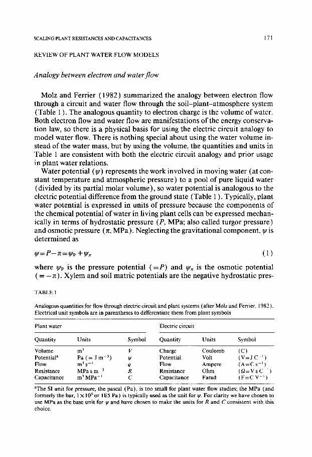
Molz and Ferrier ( 1982 ) summarized the analogy between electron flow through a circuit and water flow through the soil-plant-atmosphere system (Table 1 ). The analogous quantity to electron charge is the volume of water. Both electron flow and water flow are manifestations of the energy conserva- tion law, so there is a physical basis for using the electric circuit analogy to model water flow. There is nothing special about using the water volume in- stead of the water mass, but by using the volume, the quantities and units in Table 1 are consistent with both the electric circuit analogy and prior usage in plant water relations.
Water potential (~,) represents the work involved in moving water (at con- stant temperature and atmospheric pressure) to a pool of pure liquid water (divided by its partial molar volume), so water potential is analogous to the electric potential difference from the ground state (Table 1 ). Typically, plant water potential is expressed in units of pressure because the components of the chemical potential of water in living plant cells can be expressed mechan- ically in terms of hydrostatic pressure (P, MPa; also called turgor pressure) and osmotic pressure ( rr, MPa). Neglecting the gravitational component, ~, is determined as
t u = P - zr= ~p + ~,~ (1)
where ~,p is the pressure potential ( = P ) and ~u,~ is the osmotic potential ( = - 7r). Xylem and soil matric potentials are the negative hydrostatic pres-
TABLE 1
Analogous quantities for flow through electric circuit and plant systems (after Molz and Ferrier, 1982). Electrical uni t symbols are in parentheses to differentiate them from plant symbols
Plant water Electric circuit
Quanti ty Uni ts Symbol Quanti ty Uni ts Symbol
Volume m 3 V Charge Coulomb (C) Potential a Pa ( = J m -3) ig Potential Volt ( V = J C-1 ) F10w m 3 s - l q Flow Ampere (A = C s - l ) Resistance MPa s m -3 R Resistance Ohm (J2=V s C ~ ) Capacitance m 3 MPa-~ C Capacitance Farad (F = C V 1 )
"The SI unit for pressure, the pascal (Pa ) , is too small for plant water flow studies; the MPa (and formerly the bar, 1 × 10 3 or IE5 Pa) is typically used as the unit for ~g. For clarity we have chosen to use MPa as the base uni t for ~, and have chosen to make the units for R and C consistent with this choice.
172 E.R. HUNT, JR. ET AL.
sures exerted by surface tension effects, and should be included in the hydro- static pressure term (Nobel, 1983 ).
From the base quantities of volume and ~u, the quantities of water flow, resistance and capacitance are derived in a similar manner as the same quan- tities for electron flow (Table 1 ). However, there are limits to how far the electric circuit analogy can be extended; for example, there may not be an analogous plant inductance because the water molecule has no net charge. Hydraulic head is an alternative to water potential frequently used by agri- cultural meteorologists, hydrologists and soil scientists; the water quantities in Table 1 can be defined using head instead of potential.
Resistances and res&tivities
Not the least confusing part of this subject are the many different ways in which resistance can be and has been expressed (Table 2; after Jarvis, 1975 ). Resistance is defined as a flow rate divided by the potential difference induc- ing the flow. Its reciprocal, conductance, is also used. 'Resistance' and 'con- ductance' are used when the flow is defined as volume per time; 'resistivity' and 'conductivity' are used with flux density ( (volume/area) / t ime; Jarvis, 1975 ). Potential or head gradient resistances and resistivities are particularly important for water transport through the soil and xylem, whereas potential or head difference resistances and resistivities are useful for describing trans- port through roots and leaves. It should be pointed out that stomatal conduc-
TABLE2
Definitions of resistance and conductance with their units
Flow Flux density
Resistance Conductance Resistivity Conductivity
Potential gradient ( d~//dl)/q q/ ( d~u/dl) ( d~/dO/q q/ ( d~/dl) ( M P a s m -4) ( m 4 s - l M P a -~) ( M P a s m -2) (m2s-~MPa -~)
Potential difference 3~v/q q13 V 3VI q q/3~v ( M P a s m -3) ( m 3 s - l M P a - t ) ( M P a s m - I ) ( m s - l M P a - l )
Head gradient (dH/dl)/q q/(dH/dl) (dH/dl)/q q~ (dH/dl) ( sm -3) (m3s -1 ) ( sm - t ) ( m s - l )
Head difference 3H/q q/AH 3H/q q/3H ( sm -2) (m2s - ' ) (s) (s - ' )
Water flow in volume/t ime is q, S is surface area, ~u is potential, H is hydraulic head ~ and I is length. The ratio q/S is the volumetric flux density (q). Potential and head gradient are used for water trans- port through the xylem and soil; potential and head difference are used for transport across leaves and roots. ( ~Units for head are meters, which give a potential when multiplied by the density of water (p, 1 Mg m-3) and gravitational acceleration (g, 10 m s - 2 ) ; H of I m is equal to ~/of 0.01 M Pa. )
SCALING PLANT RESISTANCES AND CAPACITANCES 17 3
tance and resistance to the diffusion of water vapor are used with flux density, and perhaps should be called stomatal conductivity and resistivity in order to be consistent.
The relevant areas and lengths must be carefully stated. Within six lines of text, Landsberg and Fowkes ( 1978, p. 499 ) defined various 'resistances' with units of bar s m m - 1, bar s m m - 3 and bar s m m - 4 ! Bristow et al. (1984) used the potential difference resistivity per unit root length for flow into roots. This has the same units as potential gradient resistivity, but is not comparable because the length is at right angles to the flow path rather than along it. Standardization is certainly desirable; perhaps Table 2 can contribute to it.
When comparing resistivity in different parts of the system, it is important that the unit area be defined the same for all components (Richter, 1973). Resistivities in series are only additive if the area is constant. For whole-plant canopies, the area normally used is unit land surface area. Leaf area, stem cross-sectional area, stem sapwood area, xylem lumen area and root surface area have also been used to define resistivities. For individual plant studies, it may be better to use resistance than resistivity.
Electric circuit analog models
This section uses the model of Federer ( 1979, 1982 ) as a starting point for the following discussion, but the underlying theory is similar to many other model formulations. Developing some equations for the liquid flow pathways helps clarify some of the assumptions that are usually made in models of water flow. Figure 1 shows a non-steady-state model for a single plant; the same analog model is applied here to a plant stand for a given unit of land surface a r e a ( S land, m2), where the volume flows (q, m 3 s -1 ), capacitances (C, m 3 MPa -1 ) and potential difference resistances (R, MPa s m -3) are changed below to the corresponding volume flux densities (q=q/S la"d, m s-L ), capa- citivities (C=C/S land, m MPa -1) and resistivities (R, MPa s m-L) , respectively.
The root zone of a soil can be divided into several layers, each layer (i) having its own water potential in the bulk soil, ~,~oiL. Rhizosphere resistivity, ~oi,, and root resistivity to radial flow in the root, Rr r°°t, are in series in each layer (Cowan, 1965; Federer, 1979). The potential where water first enters the root xylem, ¢trx °°t, is assumed to be independent of soil layer, i.e. xylem resistivity is negligible for large roots, and hence no corresponding resistor is shown in Fig. 1. Water entering from plant stem storage at ~//s stem, through a storage resistivity Rs stem , is assumed to enter halfway along the xylem path and halfway up the height of the plant. The difference between the leaf water po- tential, ~leaf, and ~u s°iL drives the fluxes of water. The transpiration flux
174
cieaf k~#sleaf •
~ stem U s stem
soil soiI
soil soil C2 Y2
I
soil soil
I =
leaf q
L~ leaf
tem
stem
soil _ root ~ R stem R r i - - < x
;oot
soil R root R2 r2
RT' R:t °t
E.R. HUNT, JR. ET AL.
Fig. 1. Capacitances (C), potentials (~) and potential difference resistances (R) in the soil- plant-atmosphere pathway for liquid water flow using an electric circuit analog model. Symbols are C~ i' for the soil water storage of soil layer i, ~u~ °i~ for soil potential of soil layer i, R~ °il for the soil resistance in soil layer i, Rrr~ ?°t for the root radial resistance across the root surface area for roots in soil layer i, RSx tern for the resistance of the xylem from the roots to the leaves, R~ 'era for the resistance from stem water storage to the xylem, R~ ear from leaf water storage to the xylem, C stem for the stem water storage, C ~eaf for leaf water storage, ~roo, for the root xylem potential, ~x re" for the stem xylem potential, ~gs stem for the stem storage potential, ~//Iseaf for the leaf storage potential, ~/eaf for the leaf potential and q|¢af for the transpirational water flow. Units for R, C, and ~ are given in Tables 1 and 3. For a steady-state water flow model, only C~ °~, R s°ilR ~oot and R stem are used. Water from C stem is added at the midpoint ofR~x tern. The capacitors are grounded to make the charge on the capacitor equal to the water potential. Volumetric flux density (q), capacitivity (C) and resistivity (R) denote the respective quantities per land surface area.
dens i ty l eav ing the p l an t is
q = ( ~//Sxtem __ ~/gleaf __ 0 . 5 p g h )/0.5RSx t em ( 2 )
whe re p is the dens i ty o f wate r , h is the he ight a b o v e the g r o u n d a n d g is the acce le ra t ion o f gravi ty . F o r s impl ic i ty , we ignore the capac i t ance o f the leaves, wh ich is smal l c o m p a r e d wi th the c a p a c i t a n c e o f the s tem, a n d a s s u m e on ly one s torage poo l o f w a t e r in the s t e m s to o b t a i n a single p l an t capac i t ance . T h e w a t e r supp l i ed f r o m s torage , q~s tem, is
¢,om = ( __ ( 3 )
SCALING PLANT RESISTANCES AND CAPACITANCES 17 5
The storage potential, /]/stem, is then changed from flux into or out of storage by
Z~q/stem = -- (qSstem/cstem)zlt ( 4 )
where At is the time step in seconds. The total change over At must be small for eqn. (3) to be valid. Flux between/]/root and q/Sxtem is
Further simplification defines the total potential difference resistivity, R t°tal
q = (/]/soil __/]/leaf)/Rtotal (10)
w h e r e R t°tal is the sum of the plant organ resistivities and is also called the bulk plant resistivity.
Rhizosphere and root resistance
Work on resistance to transpiration in the 1960s focused on resistance to water movement through the soil to the root (Molz, 1981 ). The classic papers by Gardner ( 1960 ) and Cowan ( 1965 ) developed a theory of water flow to a single cylindrical root in which the potential difference is/]/soil minus the po- tential at the root surface, q/root, and the conductivity depends on the soil hy- draulic conductivity. The theory applies to flow per unit length of absorbing root and assumes this is measured as the length of absorbing root per unit volume of soil. The radial root resistivity, Rr r°°t, was assumed constant throughout the absorbing length and was initially thought to be small.
Newman (1969a,b) thoroughly reviewed theory and experiment compar- ing rhizosphere resistance with root resistance. The experiments generally were indirect and theoretical because q/root could not be measured. He concluded, as many others have since, that rhizosphere resistance is small with respect to root resistance when the soil is wet. In general, rhizosphere resistance is much smaller than root resistance until soil potential drops below - 0 . 1 MPa
176 E.R. HUNT, JR. ET AL.
(Gardner and Ehlig, 1962; Arya et al., 1975; Landsberg and Fowkes, 1978 ). Molz ( 1981 ) summarizes by saying "root resistance ... seems certain to dom- inate in the upper 75% of the water content range under normal rooting conditions."
The Casparian strip appears to be the major resistance to radial flow into the roots (Slatyer, 1967; Newman, 1976; Z immermann, 1983). Numerical values for root resistance are few and for a limited number of plant species. Landsberg and Fowkes ( 1978 ) gave potential difference resistivity based on root surface area of 3E6-5E8 MPa s m - 1 for several studies of wheat roots. Newman (1973) gave values on the order of 1E8 MPa s m -~ for young her- baceous plants, and Slatyer (1967) IE7 MPa s m - l for bean, oat and corn. The calculation of such resistivities is always based on assumptions that are not fully met. Root resistivities probably vary with root thickness (Hunt and Nobel, 1987a), root age and soil temperature (Tew et al., 1963; Dalton and Gardner, 1978; Running and Reid, 1980). Part of the temperature effect is the result of changing viscosity of water, but most is probably physiological change in root tissue, such as the endodermal cytoplasm (Slatyer, 1967 ).
Resistance to outflow of water from plant roots often appears to be higher than resistance to uptake (Molz and Peterson, 1976; Nobel and Sanderson, 1984; Dirksen and Raats, 1985 ). At night, in a soil that is wet at some depth and dry at another, plants can transfer water through the roots from the wet- ter soil to the drier one (Baker and Van Bavel, 1986; Richards and Caldwell, 1987 ), demonstrating that water flow can occur both in and out of roots. Many simulation models do not allow any outflow from plant roots (Molz, 1981 ) and, indeed, these models cannot balance water uptake with transpirational water loss except when outflow is not allowed. Continuing discussion on vari- able root resistance centers on metabolic (and osmotic) control (Fiscus, 1975; Dalton and Gardner, 1978; Fiscus et al., 1983; Passioura, 1984, 1988; Parker and Pallardy, 1988 ), or on root-soil interface resistance caused by an air gap that forms as the soil and root pull away from each other when the soil and root dry (Huck et al., 1970; Herkelrath et al., 1977; Dosskey and Ballard, 1980; Molz, 1981; Bristow et al., 1984).
Conversion of root resistivities based on unit surface area of the root (S r°°~, m 2 ) to resistivities based on unit land area require estimation of the length of absorbing roots per unit land area and of the diameter of the absorbing or fine roots. Roots > 1 or 2 m m in diameter may be too suberized to absorb at all, except through cracks in the suberized layer (Caldwell, 1976 ). Studies of fine root length are exceedingly tedious and so are seldom carried out in natural conditions. Values of the order of 0.35 m m radius and 10 m 2 S r°°t per m 2 S land
are likely for forests (Federer, 1979 ). Then Rr ~°°t of 1E8 MPa s m - t based on root surface area becomes 1 E7 MPa s m - l based on land area.
SCALING PLANT RESISTANCES AND CAPACITANCES 177
Xylem resistance
Different groups of plants have widely differing hydraulic architectures. Some understanding of this is needed to assess xylem resistance and conduc- tance. Separation of plants into at least eight categories in necessary, but lit- erature results for any one group are often mistakenly taken to apply to all. Also, this is probably true for root xylem resistance, but has not been studied. The groups are: (1) ferns (including tree-ferns); (2) gymnosperms (mainly coniferous trees); (3) herbaceous dicot annuals; (4) succulent dicots (in- cluding cacti); (5) woody diffuse-porous dicot trees and shrubs; (6) woody ring-porous dicot trees and shrubs; (7) grasses; (8) other monocots (includ- ing palm trees).
All groups conduct water through dead xylem cells, either vessel elements or tracheids, or both. Conifers and woody dicots have secondary cambium and produce new xylem radially in the stem each year. Tree-ferns and most monocots grow only up, not out, and must rely on the same xylem cells to function throughout the plant's life. In conifers and other primitive plants, the conducting xylem cells are tracheids, which are 20-50/ lm in diameter and 1-3 m m long; these carry water with a velocity of 1-2 m h - 1 (Zimmermann, 1983). The source of the xylem resistance is not within the tracheid lumens themselves, but in the bordered pits that connect adjacent tracheids (Jarvis, 1975; Gibson et al., 1985; Calkin et al., 1986).
In woody dicots, water is carried primarily by vessel elements, which are large diameter cells with dissolved end walls and stacked end to end to form a long continuous vessel. Vessels in diffuse porous trees are 15-150/~m in diameter, 100 m m long and carry water at 1-6 m h -~. In ring-porous trees, the vessels are 60-400 ~tm in diameter, >i 1 m long and conduct water at 6-40 m h - I. Resistance to water flow through wood can be measured by forc- ing water under pressure through a stem segment. Such work indicates that water flow is laminar and the Hagen-Poiseuille law for flow in capillaries applies (Heine, 1971; Zimmermann, 1983; Schulte et al., 1989). Water flow through a single vessel is, therefore, proportional to the fourth power of its radius. Deviations from the Hagen-Poiseuille law can be attributed to rough vessel element walls (Jeje and Zimmermann, 1979) and small variations in diameter along the length of the vessel (Schulte et al., 1989 ).
Measured potential gradient resistivities range from 200 to 30 000 MPa s m -2 for conifers and 30 to 3000 MPa s m -2 for dicot trees, based on sapwood cross-sectional area of the bole (Heine, 1971; Ewers, 1985 ). Assuming the sapwood basal area (sapwood area per tree Xthe number of trees per land area) is 20 m 2 ha -1 and the trees (either woody dicot or conifer) are 20 m tall, then 1000 MPa s m -2 potential gradient resistivity based on sapwood area converts to 1 E7 MPa s m - ~ potential difference resistivity based on land surface area. This is equal to 1 E7 MPa s m - ~ estimated above for root resis-
178 E.R. HUNT, JR. ET AL.
tivity per land surface area. Xylem resistivity in a forest is at least the same order of magnitude as root resistivity and should not be neglected (eqn. ( 9 ) ).
Comparisons of resistance on the basis of sapwood area with that of land surface area are complicated by estimation of the portion of the sapwood that is actually conducting, In conifers, conduction may vary across the sapwood, which is approximately the outer 10-20 annual rings. In diffuse-porous dicot trees, conduction decreases linearly inward over about 10 rings. In ring-po- rous trees, almost all water transport is in the outermost one or two annual rings (Waring and Schlesinger, 1985 ). In monocots, herbaceous dicots and ferns, vascular bundles are scattered throughout the stem. Stem resistivities in the literature must be evaluated to see if they are based on lumen area, conducting xylem area, sapwood area, stem area, one-sided leaf area, total leaf area or land surface area.
Many of the more recent studies determined xylem potential gradient con- ductivities per unit leaf area supplied by the xylem (called leaf-specific con- ductivities) in order to show how these conductivities vary throughout the stem (Zimmermann, 1978, 1983; Tyree et al., 1983; Ewers and Zimmer- mann, 1984a,b; Tyree, 1988). In general, boles have leaf-specific conductiv- ities about four to five times higher than the lateral minor stems, which hold most of the leaves, suggesting that these minor stems contribute most of the resistance to water flow through the xylem. Furthermore, when the potential gradient of stems and roots for a given transpiration rate is calculated from a series of water potential measurements, the largest potential drop occurs in the minor lateral stems, suggesting that these minor stems constitute the larg- est single resistance in the whole soil-plant-atmosphere system (Hellkvist et al., 1974; Zimmermann, 1983; Tyree, 1988; Tyree and Sperry, 1989). The variation in hydraulic architecture of a single tree thus presents a considera- ble challenge in formulating a single xylem resistivity.
Total resistance
The total potential difference resistivity of a plant canopy is the leaf-soil potential difference divided by the water flux density (eqn. (10)) . A great many plant canopies have ~eaf of about - 1.5 MPa when ~,soil is > -0 .1 MPa and transpirational flux density is about 0.5 mm h - 1. The potential difference resistivity thus defined is about 1 E7 MPa s m - ~, which is the same order of magnitude as the estimated xylem and root potential difference resistivities determined above. Abdul-Jabbar et al. (1984) gave values of 3E6 to 1.2E7 MPa s m-1 from the literature. Total plant resistivity varies a little among species (Boyer, 1971 ). In general, few comparisons under the same ambient conditions have been carried out, but total resistivity appears to vary less than the component resistivities. In view of the order of magnitude uncertainties
SCALING PLANT RESISTANCES AND CAPACITANCES 179
in the estimation of root and xylem resistance, the use of a whole-canopy po- tential difference resistivity seems more justified for GCM.
Capacitance
Many studies have measured instantaneous transpiration rate, ~ffleaf and ~,soil, and then estimated total plant resistance using eqn. ( 10 ); these studies have generally concluded that R t°tal or R tot,~ varies diurnally with flow rate. These studies also have generally ignored the effects of plant capacitance. Although plant resistances do change from osmotic effects (Fiscus et al., 1983; Pas- sioura, 1984, 1988 ), plant growth (Boyer, 1985 ), stem water content (Ed- wards and Jarvis, 1982 ) and xylem embolism (Tyree and Dixon, 1986; Sperry et al., 1988a,b; Tyree and Sperry, 1988, 1989), These changes are more im- portant over a season than over a day (however, see Passioura and Tanner, 1985 ). Over a day, plots of the variation in transpiration rate of ~/eaf form a hysteresis loop (Jarvis, 1975; Hinckley et al., 1978; Schulze et al., 1985). Constant plant capacitance with constant plant resistance can fully explain the daily hysteresis between transpiration and ~,leaf (Hinckley et al., 1978; Jones, 1978; Waring and Running, 1978; Running, 1980a; Wronski et al., 1985; Katerji et al., 1986; Hunt and Nobel, 1987a; Tyree, 1988).
Following the electric circuit analogy, capacitance (C) is defined as
C=dV/d~, (11)
where V is the volume of water. Capacitance may be determined from the slope of a pressure-volume curve (Powell and Thorpe, 1977; Waring and Running, 1978; Running, 1980a; Tyree and Jarvis, 1982). The slope of a pressure-volume curve is not constant throughout its range, therefore capac- itance is not constant. However, the initial slope of a pressure-volume curve is approximately constant over a range of relative water content (RWC) from 0.95 to 0.80. RWC is defined as V/Vo, where Vo is the volume at ~,=0 MPa. Most measured ~v in the field are usually within this range of RWC. Moreover, soil-moisture release curves show that C s°il is not constant, but the change in volumetric water content over a day is small. Therefore, as a first approxi- mation, constant plant and soil capacitances may be used for modeling diur- nal water flow through the soil-plant-atmosphere system.
For plant tissues of living cells, the bulk elastic modulus (E, MPa) of a tissue is defined as VdP/dV and controls the initial slope of the pressure- volume curve (Molz and Ferrier, 1982; Tyree and Jarvis, 1982). For the range covered by the initial slope
C= V/ (e+ zr) (12)
which shows that larger plants will have larger capacitance simply because they have a larger volume of water in living cells. Equation ( 12 ) follows from
180 E.R. HUNT, JR. ET AL.
differentiating eqn. ( 1 ) with respect to volume, eqn. ( 11 ), the definition of e, and assuming no change of total osmotically active solutes so dn/dV= -nlV.
One typical non-steady-state model is shown in Fig. 1, where each plant organ is modeled as a single grounded capacitor connected to the xylem resis- tance catena through a storage resistor. Similar models were used by other investigators (Landsberg et al., 1976; Powell and Thorpe, 1977; Jones, 1978; Wronski et al., 1985; Edwards et al., 1986), and particularly by Nobel and collaborators, to investigate capacitance as functional adaptations to desert environments (Nobel and Jordan, 1983; Hunt and Nobel, 1987a; Schulte and Nobel, 1989).
The resistance-capacitance circuit analog in Fig. 1 is complicated enough to represent the dynamics of water flow through each plant organ, but simple enough to be solved analytically (e.g. Powell and Thorpe, 1977; Wronski et al., 1985 ). The parameters for such a model are determined from combining many small resistances and capacitances determined for an individual plant in parallel or in series. If the electric circuit analog is taken literally, then more complicated models can be solved using available electric circuit simulation programs (Molz et al., 1979 ). One such program accurately predicted diurnal variations of Ceaf using the same plant resistances and capacitances for both wet and dry soil (Hunt and Nobel, 1987a). Leaf capacitance is small, but is important for the prediction of ~//leaf and subsequently the driving force for water flow through the soil-plant-atmosphere system. At the minimum, dy- namics of water flow through a whole plant can be represented using a single capacitor and one or two resistors (Jones, 1978; Milne et al., 1983; Wronski et al., 1985).
There are three pools of stored water in the stems of woody plants. The first pool is in the living cells of the xylem parenchyma, cambium and phloem; this pool of stored water changes diurnally and is responsible for diurnal changes of stem diameter (Dobbs and Scott, 1970; Lassoie, 1973, 1979; Jar- vis, 1975).
The second pool is in the lumens of the conducting xylem tissue and changes seasonally (Clark and Gibbs, 1957; Dobbs and Scott, 1970) owing to cavita- tion (breakage of the water column) and embolism (entry of air into the lu- men; Tyree and Sperry, 1988). Cavitation and embolism require positive pressures of water in the xylem to be reversed, which occurs during the spring if at all. It is unlikely that reversal can occur overnight. The seasonal change of the second pool of stored water is from 2 mm (Roberts, 1976) to a maxi- mum of 27 mm (Waring and Running, 1978). However, for most forest stands, the seasonal change of xylem lumen water is probably < 10 ram, so this pool can be neglected in soil-plant-atmosphere models simulating diur- nal water flow.
The third pool is water bound in the cell walls of the xylem tissue, where
SCALING PLANT RESISTANCES AND CAPACITANCES 181
the water potential is equal to the negative hydrostatic pressure and is in equi- librium with the potential of the other two pools. In a significant study, Brough et al. (1986) showed that only 5% of the diurnal changes of stem water con- tent can be attributed to the first pool in living cells, most of the diurnal change in stem water is from the third pool. Thus, it is the third pool of stored water that acts as the single stem capacitor in non-steady-state models of water flow.
AN A L Y SI S O F W A T E R F L O W M O D E L S AT V A R I O U S H I E R A R C H I C A L SCALES
Steady-state versus non-steady-state models
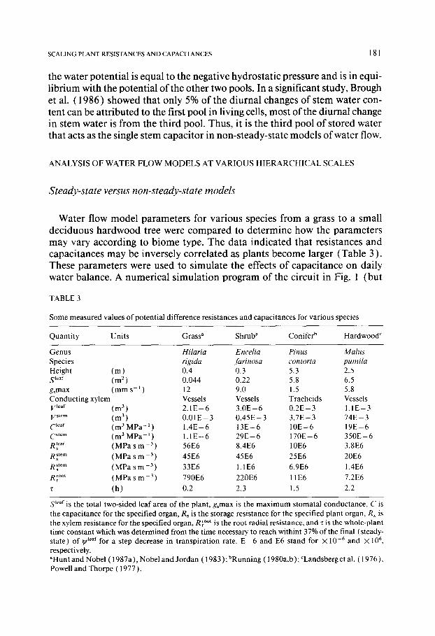
Water flow model parameters for various species from a grass to a small deciduous hardwood tree were compared to determine how the parameters may vary according to biome type. The data indicated that resistances and capacitances may be inversely correlated as plants become larger (Table 3 ). These parameters were used to simulate the effects of capacitance on daily water balance. A numerical simulation program of the circuit in Fig. 1 (but
TABLE 3
Some measured values o f potential difference resistances and capacitances for various species
Quanti ty Uni ts Grass a Shrub a Conifer b Hardwood c
Genus Hilaria Encelia Pinus Malus Species rigida farinosa contorta pumila Height ( m ) 0.4 0.3 5.3 2.5 S lear (m 2) 0.044 0.22 5.8 6.5 gsmax ( m m s -~ ) 12 9.0 1.5 5.8 Conduct ing xylem Vessels Vessels Tracheids Vessels V l~af (m 3 ) 2 . 1 E - 6 3 . 0 E - 6 0 . 2 E - 3 I . I E - 3 V stem (m 3 ) 0 . 0 1 E - 3 0 . 4 5 E - 3 3 . 7 E - 3 7 4 E - 3 C leaf ( m 3 M P a - l ) 1.4E - 6 1 3 E - 6 10E - 6 19E - 6 C stem (m 3 MPa - I ) 1 . 1 E - 6 2 9 E - 6 1 7 0 E - 6 3 5 0 E - 6 R~ ear (MPa s m -3) 56E6 8.4E6 10E6 3.8E6
Rs stem (MPa s m 3) 45E6 45E6 25E6 20E6 RSx tern (MPa s m -3) 33E6 1.1 E6 6.9E6 1.4E6
R~ °°' (MPa s m -3) 790E6 220E6 11E6 7.2E6
r (h ) 0.2 2.3 1.5 2.2
S leaf is the total two-sided leaf area o f the plant, gsmax is the max i mum stomatal conductance, C is the capacitance for the specified organ, Rs is the storage resistance for the specified plant organ, Rx is the xylem resistance for the specified organ, R root is the root radial resistance, and r is the whole-plant time constant which was determined from the t ime necessary, to reach withint 37% of the final (steady- state) o f q/leaf for a step decrease in t ranspirat ion rate. E - 6 and E6 stand for X l0 -6 and X l06, respectively. aHunt and Nobel ( 1987a ), Nobel and Jordan ( 1983 ); bRunning ( 1980a,b ); CLandsberg et al. ( 1976 ), Powell and Thorpe (1977).
182 E.R. HUNT, JR. ET AL.
with only one soil layer) was used to estimate water potentials and water flows at a given transpiration rate and ~o~ for both the steady-state (resistor circuit analog) and non-steady-state (resistor-capacitor circuit analog) models.
The differences between a steady-state model and a non-steady-state model are very significant over a day (Fig. 2 ). The main effects of adding capaci- tance are the higher ~ a f and lower maximum instantaneous rate of water uptake. Moreover, minimum (//leaf lagged behind maximum transpiration rate by 1 h for Encelia farinosa (Fig. 2 (B) ). Simulations of a plant with a small capacitance, such as a grass (Hilaria rigida), show little lag when capacitance
T <
54 CO
g 4
°i1 c
°1 ~- o o
(A) Steady state ;
/
/ 6
,af water potential
anspiration and uptake
1 '2 1 '8 2'4
n
-0.5 E O o_
-1.5 30
< to
¢o <
E g
t~
~=
.o_ =
t --
6- 0 \ (B) Non-steady state f z ~ - ~
5- \ /
A 4- / ~ / Leaf water potential --0.5 -~
z
3- F ranspiration f / ~ ~
21 l / / ' Uptake -I "~
0 ~ , - 1 . 5 0 6 12 18 24 30 Time (hours after midnight)
Fig. 2. Simulated transpiration rate, rate of water uptake by roots and leaf water potential for E. farinosa using a steady-state model (A) or non-steady-state model (B). Model parameters for E. farinosa are given in Table 3. The transpiration rate was calculated from the Penman- Monteith equation for a warm August day in Missoula, MT, where stomatal conductance was determined from maximum conductance, solar radiation, vapor pressure difference and ~,soi~ = _ 0.1 MPa. For both (A) and (B), total daily water uptake by the roots equals total daily water loss by transpiration. Moreover, the daily totals and instantaneous rates of transpiration for the steady-state model are the same as those for the non-steady-state model because stomatal conductance was not controlled by ~u jear.
S C A L I N G P L A N T R E S I S T A N C E S A N D C A P A C I T A N C E S 183
is introduced. Simulations of plants with large capacitances and small resis- tances, such as a lodgepole pine or an apple tree, have a slightly smaller lag period than E. farinosa. Use of a steady-state model will give reasonable pre- dictions of Iff leaf for a grassland, but predictions of ~leaf using the same steady- state model with resistances accurately parameterized for a forest will be in error because of a considerable lag period.
The simulation results (Fig. 2 ) show another important point; total daily transpiration is nearly equal to total daily water uptake by the roots for both the steady-state and non-steady-state water flow models; inclusion of capaci- tance has no practical effect on daily totals. Running ( 1984 ) showed the same point for forest stands by comparing one simulation model, H2OTRANS, which uses hourly time steps and capacitance terms, with another simulation model, DAYTRANS, which uses daily time steps and no plant capacitance terms. Over a growing season, the DAYTRANS predictions were almost iden- tical to those of H2OTRANS for cumulative transpiration and soil water de- pletion (Fig. 3). Moreover, the predictions of soil water depletion by both models were similar to measured soil water depletion.
Thus, non-steady-state models with plant capacitance are necessary for pre- dicting diurnal variations of water uptake by the roots and leaf water poten- tial, but steady-state models without plant capacitance suffice for predicting
"o
(,9
200-
150-
100-
I soj 0 ' , . . . . . 120 140 160 180 200 220 240
Day of year
00
150 ~E
-100 "~ .~.
I-- 50
0 260
Fig. 3. Comparison of hourly time resolution water flow model with capacitance with daily time resolution model without capacitance over a growing season. Simulations compare H2OTRANS (hourly time step) and DAYTRANS (daily time step) numerical results to observe data on lodgepole pine at the Frasier Experimental Forest (CO, USA) during the summer of 1978. Symbols are: simulated cumulative transpiration by H2OTRANS ([] ) and by DAYTRANS ( • ), simulated soil water depletion by H2OTRANS ( + ) and by DAYTRANS ( × ), and mea- sured soil water depletion ( • ) . Soil water depletion from a maximum soil water content of 250 mm was measured using a neutron probe; there were no observed data for transpiration. For seasonal and annual simulations, daily time steps appear adequate for modeling transpiration and soil water depletion (Running, 1984).
184 E.R. HUNT, JR. ET AL.
daily and seasonal totals o f t r ansp i ra t ion and water uptake. In general, for any spatial area f rom individual plants to large forest stands, the choice o f a steady- state or non-s teady-s ta te mode l is dependen t on the model ' s t ime resolut ion and purpose.
Plant water flow time constants
One m e t h o d for de te rmin ing the necessity o f capaci tance for so i l - p l an t - a tmosphere models is the compar i son of a mode led t ime cons tan t wi th the mode l t ime step (Allen and Starr, 1982; O'Nei l l et al., 1986). T ime constants can be def ined using the electric circuit analogy. For a resistor and capaci tor in series, the t ime cons tan t (z, s ) is equal to the p roduc t o f the resistance and the capacitance. Thus, z for water flow into and out o f storage in the s tem is equal to resistance to and f rom storage (R stem) mul t ip l ied by C stem (Fig. 1 ). Comple te response to a step change in potent ia l is usually said to have oc- curred after 3~. W h e n the mode l t ime step is about equal to r, capaci tance mus t be inc luded in water flow models .
A whole-plant z can be de f ined as the length o f t ime necessary to reach 63% (exp -1 ) o f the final s teady-state value for a step change in condi t ions . Using the same resistances for a series o f s imula t ions (smal l resistances tha t are appropr ia te for a large t ree) , C stem was var ied f rom 1 to 1000 m 3 M P a - 1 and
1o0000! ~1ooooo T r e ~
~ 10000i~ y I10000 ~ .
oo t ooo ~ - / ~ hrub 1000 o
loo ~ lOO
E Grass .--- o 10 10 "~ O uJ
l i 10 100 100(
Capacitance (m ̂ 3 MPa ̂ -1)
Fig. 4. Relationship of whole-plant time constant (r) with stem capacitance for a step decrease in transpiration rate (computed z, [] ) and for the product of (R~ °°~ +0.5RSx tern + R ~ tern ) and C ~tem (estimated r, • ). Resistances and transpiration rate were the same for each numerical simulation: ~,soi~= -0.1 MPa, R~°°t = 10E6 MPa s m-3, Rstem =2E6 MPa s m-3, Rstern= 10E6 MPa s m- 3 R ~eaf= 5E6 MPa s m -3 and Clear= 1 E -6 m 3 MPa -I. The resistances are appropri- ate for large plants (large C stem, small R), the whole-plant z will be greater with larger resis- tances, which are appropriate for smaller plants (small Cstem). Thus, these simulations indicate the minimum r that would be expected for a given biome from grasslands to forests.
SCALING PLANT RESISTANCES AND CAPACITANCES 18 5
z was determined by following ~//leaf for a step decrease of transpiration rate (Fig. 4). The increase in z was from about 20 s for the smallest capacitance to 6 h for the largest capacitance (Fig. 4), which is smaller than a grass and larger than a very large tree, respectively. Whole-plant z was approximately equal to the product of (Rr ~°°t -~-0.5R stem "~-R stem ) and C stem (Fig. 4). For a step increase in transpiration rate, z varied from about 10 s to 3 h over the same range of capacitance, and was about equal to the product of
stem stem c s t e m (0.5Rx + R~ ) and The step decrease in rate determines the amount of lag and hysteresis, whereas the step increase in rate determines how fast the plant will respond to sunrise.
The resistances of real plants vary with plant size, where S ~°°t increases with S leaf and causes R r°°t to decrease, so increases of C ~t~m with increases of plant size do not mean that z will automatically increase. In Table 3, z was about equal for the shrub, E. farinosa, the lodgepole pine and the apple tree. Whole-plant z was still about equal to the product of ( R r°°t q-0.5RSx tem "t-R stem ) and C stem for a step decrease in transpiration rate. These simulations (Fig. 4; Table 3) show the need to accurately determine non-steady-state model parameters for different-sized plants.
Ecosystem time constants
Capacitances in parallel are additive, whereas resistances in parallel are added by reciprocals. So, if n plants were n parallel paths in an electric circuit for an entire ecosystem, then based on whole-plant z being about equal to (R r ~°°t + 0.5R Sxtem + R ~tem ) × cl~af from above, an ecosystem time constant (z) may be defined using an 'average plant' as
z= (n C stem ) / [n/(R~ °°t -~- 0.5R Sx tem q-R stem ) ] ( 13 )
which is equal to z of the whole plant. This does not mean that C stem, Rstem R s t e m and R r ° ° t for individual plants equal the respective quantities
x , ~ s ~ r
cstem ]~stem Rstem and R r°°t for ecosystem models; these quantities are equally , - = x 9 ~ i s
scaled by the number of plants per land surface area to determine ecosystem 2".
Allometric relationships are of the form log y = a + b log x and are generally used to estimate some size variable from another easily measured size vari- able (i.e. tree volume from tree diameter) . The area of sapwood xylem in a stem cross-section is aUometrically related to leaf area index (LAI .~-sleaf/sland, m 2 m -E) for many different species (Waring, 1983; Waring and Schlesinger, 1985 ). Inverting allometric relationships between LAI and sapwood area may be used to estimate R~x t~m. However, the allometric equations relating LAI and xylem sapwood area have considerable variations among species (Waring, 1983; Waring and Schlesinger, 1985 ) and within a single species owing to stand age, health and density (Pothier et al., 1989).
186 E.R. H U N T , JR. ET AL
E
J
lal kv ! t
SCALING PLANT RESISTANCES AND CAPACITANCES 18 7
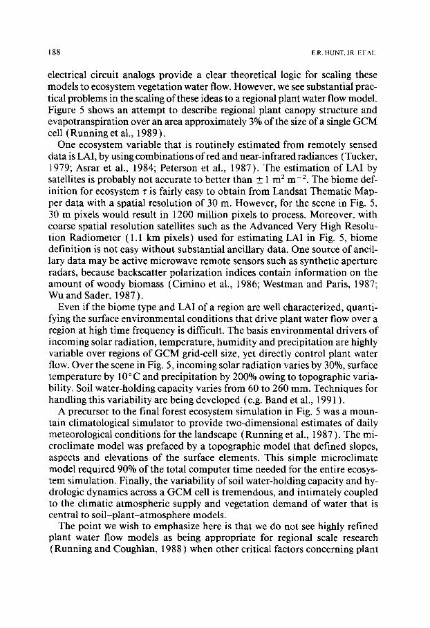
Fig. 5. Region diagram (a), total leaf area index (b) and annual evapotranspiration (c) of the Flathead and Seely-Swan valleys in northwestern Montana (USA) after Running et al. (1989). The area covered is 28 X 55 km; the 1.1 km grid cell was defined by the NOAA/AVHRR sensor. The region diagram (a) shows prominent physiographic features, average elevation of moun- tain ranges (scale left) and annual precipitation (black bars, scale right). Leaf area index was determined using NOAA/AVHRR sensor data, transpiration was estimated using the models of Running et al. (1987) and Running and Coughlan (1988).
Moreover, sr°° t /S land may be allometrically related to LAI and may be use- ful in estimating R r°°t. Allometric relationships between root and leaf surface area have been found for many species (Fiscus and Markhart , 1979; Fiscus, 1981; Kummerow, 1983; Hun t and Nobel, 1987b; Van Praag and Weissen, 1988 ); however, these allometric relationships contain variation of as much as an order of magnitude. Thus, it is unlikely that allometric relationships based on LAI can be used to accurately parameterize so i l -p lan t -a tmosphere models for single ecosystems. An easier alternative at present would be to use the whole-plant z in Fig. 4 for a given b iome type grassland, shrubland and forest as the ecosystem z.
Implementation of plant water flow models for large spatial scales
We have illustrated the fact that so i l -p lan t -a tmosphere models of water flow through single plants are well developed. Additionally, we showed that
188 E.R. HUNT, JR. ET AL.
electrical circuit analogs provide a clear theoretical logic for scaling these models to ecosystem vegetation water flow. However, we see substantial prac- tical problems in the scaling of these ideas to a regional plant water flow model. Figure 5 shows an attempt to describe regional plant canopy structure and evapotranspiration over an area approximately 3% of the size of a single GCM cell (Running et al., 1989).
One ecosystem variable that is routinely estimated from remotely sensed data is LAI, by using combinations of red and near-infrared radiances (Tucker, 1979; Asrar et al., 1984; Peterson et al., 1987). The estimation of LAI by satellites is probably not accurate to better than _ 1 m 2 m -2. The biome def- inition for ecosystem z is fairly easy to obtain from Landsat Thematic Map- per data with a spatial resolution of 30 m. However, for the scene in Fig. 5, 30 m pixels would result in 1200 million pixels to process. Moreover, with coarse spatial resolution satellites such as the Advanced Very High Resolu- tion Radiometer ( l . l km pixels) used for estimating LAI in Fig. 5, biome definition is not easy without substantial ancillary data. One source of ancil- lary data may be active microwave remote sensors such as synthetic aperture radars, because backscatter polarization indices contain information on the amount of woody biomass (Cimino et al., 1986; Westman and Paris, 1987; Wu and Sader, 1987 ).
Even if the biome type and LAI of a region are well characterized, quanti- fying the surface environmental conditions that drive plant water flow over a region at high time frequency is difficult. The basis environmental drivers of incoming solar radiation, temperature, humidity and precipitation are highly variable over regions of GCM grid-cell size, yet directly control plant water flow. Over the scene in Fig. 5, incoming solar radiation varies by 30%, surface temperature by 10 ° C and precipitation by 200% owing to topographic varia- bility. Soil water-holding capacity varies from 60 to 260 mm. Techniques for handling this variability are being developed (e.g. Band et al., 1991 ).
A precursor to the final forest ecosystem simulation in Fig. 5 was a moun- tain climatological simulator to provide two-dimensional estimates of daily meteorological conditions for the landscape (Running et al., 1987 ). The mi- croclimate model was prefaced by a topographic model that defined slopes, aspects and elevations of the surface elements. This simple microclimate model required 90% of the total computer time needed for the entire ecosys- tem simulation. Finally, the variability of soil water-holding capacity and hy- drologic dynamics across a GCM cell is tremendous, and intimately coupled to the climatic atmospheric supply and vegetation demand of water that is central to soil-plant-atmosphere models.
The point we wish to emphasize here is that we do not see highly refined plant water flow models as being appropriate for regional scale research (Running and Coughlan, 1988) when other critical factors concerning plant
SCALING PLANT RESISTANCES AND CAPACITANCES | 89
water flow are treated so coarsely. A basic principle of efficient systems mod- eling is that each component be modeled to an approximately equivalent level of complexity. Thus, an ecosystem z may be the only practical method of in- cluding models of non-steady-state water flow through plants into GCM.
WHAT IS THE P U R P O S E O F PLANT WATER FLOW MODELS IN GCM?
Global climate models need accurate predictions of diurnal variations of transpiration rate and soil water evaporation rate over vegetated land sur- faces (Dickinson et al., 1986; Sellers et al., 1986; Dickinson, 1987; Sellers and Darman, 1987 ). So, models of water flow through the soi l-plant-atmosphere system should be added to GCM only if they make predictions of stomatal conductance (gs, m m s - l ) , and hence diurnal variations of transpiration rate, more accurate.
Global climate models use very large spatial scales and short t ime steps (BATS/CCM 1 models use about 5 ° latitude × 5 ° longitude and a 1800 s t ime step, respectively; Dickinson et al., 1986 ). If GCM require predictions of ~eaf for the estimation of gs, then non-steady-state water flow models would be needed or errors would occur over a diurnal cycle. The errors would be large when GCM that were validated using grasslands (where z << t ime step) are applied to forests (where z> t ime step; Fig. 4). Yet, the daily totals of tran- spiration and water uptake by the roots should agree with measured hydrol- ogic balances for both forests and grasslands, as discussed above.
The main question is whether prediction of ~b ¢leaf is necessary for the predic- tion of stomatal conductance and, thus, transpiration. Recent studies on the relationship between plant water status and g~ have concluded that q/~o, and vapor pressure difference (VPD), but not ~,lear, are the significant variables controlling gs under normal conditions (Bates and Hall, 1981; Gollan et al., 1986; Schulze, 1986). The use of pre-dawn ~t leaf for the control of gs from earlier studies is consistent with this interpretation (because pre-dawn ~b ¢leaf is nearly equal to ~soil); hence, soil water variables were used indirectly to drive soil-plant-atmosphere models (Federer, 1979, 1982; Running, 1980b). When the leaf reaches ~,p = 0 MPa, ~//leaf m a y control g~ by releasing various plant hormones, but this needs more study (Schulze, 1986 ). If seasonal and diurnal variations ofgs can be accurately predicted from max imum g . VPD and ~b ¢s°il, without estimating ~leaf then we see no compelling reason for using either a steady-state model or a non-steady-state model of water flow in a GCM.
A C K N O W L E D G M E N T S
This paper was written as a direct result of a workshop on stomatal resis- tance held at Pennsylvania State University, 10-13 April 1989. The work-
190 E.R. HUNT, JR. ET AL.
shop was m a d e poss ib le p r i nc ipa l l y t h r o u g h a g ran t f r o m the N a t i o n a l Science F o u n d a t i o n ( B S R - 8 8 2 2 1 6 4 ).
We t h a n k Drs . T o b y C a r l s o n a n d J o h n Pr ice for o rgan iz ing the w o r k s h o p , at wh ich these ideas were first d iscussed . We t h a n k Dr. Mel T y r e e a n d an a n o n y m o u s r e v i e w e r for sugges t ions on the m a n u s c r i p t . F u n d i n g was pro- v i d e d in pa r t b y a N a t i o n a l Science F o u n d a t i o n g ran t to T. Ca r l son a n d J. Pr ice , a n d b y N A S A gran t N A G W - 2 5 2 to S.W. Runn ing .
REFERENCES
Abdul-Jabbar, A.S., Lugg, D.G., Sams, T.W. and Gay, L.W., 1984. A field study of plant resis- tance to water flow in alfalfa. Agron. J., 76: 765-769.
Allen, T.F.H. and Starr, T.B., 1982. Hierarchy, Perspectives for Ecological Complexity. The University of Chicago Press, Chicago, IL, 310 pp.
Arya, L.M., Blake, G.R. and FarreU, D.A., 1975. A field study of soil water depletion patterns in presence of growing soybean roots: III. Rooting characteristics and root extraction of soil water. Soil Sci. Soc. Am. Proc., 39: 437-444.
Asrar, G., Fuchs, M., Kanemasu, E.T. and Hatfield, J.L., 1984. Estimating absorbed photosyn- thetic radiation and leaf area index from spectral reflectance in wheat. Agron. J., 76: 300- 306.
Baker, J.M. and van Bavel, C.H.M., 1986. Resistance of plant roots to water loss. Agron. J., 78: 641-644.
Band, L.E., Peterson, D.L., Running, S.W., Dungan, J. Lathrop, R., Coughlan, J., Lammers, R. and Pierce, L., 1991. Forest ecosystem processes at the watershed scale: 1. Basis for distrib- uted simulation. Ecol. Model., in press.
Bates, L.M. and Hall, A.E., 1981. Stomatal closure with soil water depletion not associated with changes in bulk leaf water status. Oecologia (Berlin), 50: 62-65.
Boyer, J.S., 1971. Resistance to water transport in soybean, bean, and sunflower. Crop Sci., 11: 403-407.
Boyer, J.S., 1985. Water transport. Annu. Rev. Plant Physiol., 36:473-516. Bristow, K.L., Campbell, G.S. and Calissendorff, C., 1984. The effects of texture on the resis-
tance to water movement within the rhizosphere. Soil Sci. Soc. Am. J., 48: 266-270. Brough, D.W., Jones, H.G. and Grace, J., 1986. Diurnal changes in water content of the stems
of apple trees, as influenced by irrigation. Plant Cell Environ., 9: 1-7. Caldwell, M.M., 1976. Root extension and water absorption. In: O.L. Lange, L. Kappen and
E.-D. Schulze (Editors), Water and Plant Life. Problems and Modern Approaches. Springer- Verlag, Berlin, pp. 63-85.
Calkin, H.W., Gibson, A.C. and Nobel, P.S., 1986. Biophysical model of xylem conductance in tracheids of the fern Pteris vittata. J. Exp. Bot., 37: 1054-1064.
Cimino, J.B., Brandani, A., Casey, D., Rabassa, J. and Wall, S.D., 1986. Multiple incidence angle SIR-B experiment over Argentina: mapping of forest units. IEEE Trans. Geosci. Re- mote Sensing, GE-24: 498-509.
Clark, J. and Gibbs, R.D., 1957. Studies in tree physiology. IV. Further investigations of sea- sonal changes in moisture content of certain Canadian forest trees. Can. J. Bot., 35: 219- 253.
Cowan, I.R., 1965. Transport of water in the soil-plant-atmosphere system. J. Appl. Ecol., 2: 221-239.
SCALING PLANT RESISTANCES AND CAPACITANCES 191
Cowan, I.R., 1972. Oscillations in stomatal conductance and plant functioning associated with stomatal conductance: observations and a model. Planta, 106:185-219.
Dalton, F.N. and Gardner, W.R., 1978. Temperature dependence of water uptake by plant roots. Agron. J., 70: 404-406.
Dickinson, R.E., 1987. Evapotranspiration in global climate models. Adv. Space Res., 7: 17- 26.
Dickinson, R.E., Henderson-Sellers, A., Kennedy, P.J. and Wilson, M.F., 1986. Biosphere-At- mosphere Transfer Scheme (BATS) for the NCAR Community Climate Model. Natl. Cent. Atmos. Res. Tech. Note NCAR/TN-275 + STR, Boulder, CO, 69 pp.
Dirksen, C. and Raats, P.A.C., 1985. Water uptake and release by alfalfa roots. Agron. J., 77: 621-626.
Dobbs, R.C. and Scott, R.M., 1970. Distribution of diurnal fluctuations in stem circumference of Douglas-fir. Can. J. For. Res., 1: 80-83.
Dosskey, M.G. and Ballard, T.M., 1980. Resistance to water uptake by Douglas-fir seedlings in soil of different texture. Can. J. For. Res., 10: 530-534.
Edwards, W.R.N. and Jarvis, P.G., 1982. Relations between water content, potential and permeability in stems of conifers. Plant Cell Environ., 5:271-277.
Edwards, W.R.N., Jarvis, P.G., Landsberg, J.J. and Talbot, H., 1986. A dynamic model for studing flow of water in single trees. Tree Physiol., 1: 309-324.
Ewers, F.W., 1985. Xylem structure and water conduction in conifer trees, dicot trees, and lianas. IAWA Bull., 6:309-317.
Ewers, F.W. and Zimmermann, M.H., 1984a. The hydraulic architecture of eastern hemlock (Thuga canadensis). Can. J. Bot., 62: 940-946.
Ewers, F.W. and Zimmermann, M.H., 1984b. The hydraulic architecture of balsam fir (Abies balsamea). Physiol. Plant., 60: 453-458.
Federer, C.A., 1979. A soil-plant-atmosphere model for transpiration and availability of soil water. Water Resour. Res., 15: 555-562.
Federer, C.A., 1982. Transpirational supply and demand: plant, soil, and atmospheric effects evaluated by simulation. Water Resour. Res., 18: 355-362.
Fiscus, E.L., 1975. The interaction between osmotic- and pressure-induced water flow in plant roots. Plant Physiol., 55:917-922.
Fiscus, E.L., 1981. Analysis of the components of area growth of bean root systems. Crop Sci., 21: 909-913.
Fiscus, E.L. and Markhart, A.H., 1979. Relationships between root system water transport properties and plant size in Phaseolus. Plant Physiol., 64: 770-773.
Fiscus, E.L., Klute, A. and Kaufmann, M.R., 1983. An interpretation of some whole plant water transport phenomena. Plant Physiol., 71: 810-817.
Gardner, W.R., 1960. Dynamic aspects of water availability to plants. Soil Sci., 89:63-73. Gardner, W.R. and Ehlig, C.F., 1962. Impedance to water movement in soil and plant. Science,
138: 522-523. Gibson, A.C., Calkin, H.W. and Nobel, P.S., 1985. Hydraulic conductance and xylem structure
in tracheid-bearing plants. IAWA Bull., 6: 293-302. Gollan, T., Passioura, J.B. and Munns, R., 1986. Soil water status affects the stomatal conduc-
tance of fully turgid wheat and sunflower leaves. Aust. J. Plant Physiol., 13: 459-64. Gradmann, H., 1928. Untersuchungen fiber die Wasserverh~iltnisse des Bodens als Grundlage
des Pflanzenwachstums I. Jahrb. Wiss. Bot., 69:1-100 (in German). Heine, R.W., 1971. Hydraulic conductivity in trees. J. Exp. Bot., 22:503-511. Hellkvist, J., Richards, G.P. and Jarvis, P.G., 1974. Vertical gradients of water potential and
tissue water relations in sitka spruce trees measured with the pressure chamber. J. Appl. Ecol., 11: 637-667.
192 E,R. HUNT, JR. ET AL.
Herkelrath, W.N., Miller, E.E. and Gardner, W.R., 1977. Water uptake by plants: II. The root contact model. Soil Sci. Soc. Am. J., 41: 1039-1043.
Hinckley, T.M., Lassoie, J.P. and Running, S.W., 1978. Temporal and spatial variations in the water status of forest trees. For. Sci. Monogr., 20: 1-72.
Huck, M.G., Klepper, B. and Taylor, H.M., 1970. Diurnal variations in root diameter. Plant Physiol., 45: 529-530.
Hunt, E.R. and Nobel, P.S., 1987a. Non-steady-state water flow for three desert perennials with different capacitances. Aust. J. Plant Physiol., 14: 363-375.
Hunt, E.R. and Nobel, P.S., 1987b. Allometric root/shoot relationships and predicted water uptake for desert succulents. Ann. Bot., 59:571-577.
Jarvis, P.G., 1975. Water transfer in plants. In: D.A. DeVries and N.H. Afgan (Editors), Heat and Mass Transfer in the Biosphere. Part I. Transfer Processes in the Plant Environment. Scripta, Washington, DC, pp. 369-394.
Jeje, A.A. and Zimmermann, M.H., 1979. Resistance to water flow in xylem vessels. J. Exp. Bot., 30: 817-827.
Jones, H.G., 1978. Modelling diurnal trends of leaf water potential in transpiring wheat. J. Appl. Ecol., 15: 613-626.
Katerji, N., Hallaire, M., Menoux-Boyer, Y. and Durand, B., 1986. Modelling diurnal patterns of leaf water potential in field conditions. Ecol. Model., 33:185-203.
Kramer, P.J., 1937. The relation between rate of transpiration and rate of absorption of water in plants. Am. J. Bot., 24: 10-15.
Kramer, P.J., 1938. Root resistance as a cause of the absorption lag. Am. J. Bot., 25:110-113. Kummerow, J., 1983. Root surface/leaf area ratios in arctic dwarf shrubs. Plant Soil, 71: 395-
198 pp. Landsberg, J.J. and Fowkes, N.D., 1978. Water movement through plant roots. Ann. Bot., 42:
493-508. Landsberg, J.J., Blanchard, T.W. and Warrit, B., 1976. Studies on the movement of water through
apple trees. J. Exp. Bot., 27: 579-596. Lang, A.R.G., Klepper, B. and Cumming, M.J., 1969. Leaf water balance during oscillation of
stomatal aperture. Plant Physiol., 44: 826-830. Lassoie, J.P., 1973. Diurnal dimensional fluctations in a Douglas-fir stem in response to tree
water status. For. Sci., 19: 251-255. Lassoie, J.P., 1979. Stem dimensional fluctuations in Douglas-fir of different crown classes.
For. Sci., 25: 132-144. Milne, R., Ford, E.D. and Deans, J.D., 1983. Time lags in the water relations of Sitka spruce.
For. Ecol. Manage., 5: 1-25. Molz, F.J., 1981. Models of water transport in the soil-plant system: a review. Water Resour.
Res., 17: 1245-1260. Molz, F.J. and Ferrier, J.M., 1982. Mathematical treatment of water movement in plant cells
and tissue: a review. Plant Cell Environ., 5:191-206. Molz, F.J. and Peterson, C.M., 1976. Water transport from roots to soil. Agron. J., 68: 901-904. Molz, F.J., Kerns, D.V., Peterson, C.M. and Dane, J.H., 1979. A circuit analog model for study-
ing quantitative water relations of plant tissues. Plant Physiol., 64:712-716. Newman, E.I., 1969a. Resistance to water flow in soil and plant. I. Soil resistance in relation to
amounts of root: theoretical estimates. J. Appl. Ecol., 6: 1-12. Newman, E.I., 1969b. Resistance to water flow in soil and plant. II. A review of experimental
evidence on the rhizosphere resistance. J. Appl. Ecol., 6:261-272. Newman, E.I., 1973. Permeability to water of the roots of five herbaceous species. New Phytol.,
72: 547-555.
SCALING PLANT RESISTANCES AND CAPACITANCES 193
Newman, E.I., 1976. Water movement through root systems. Philos. Trans. R. Soc. London Ser. B, 273: 463-478.
Nobel, P.S., 1983. Biophysical Plant Physiology and Ecology. Freeman, San Francisco, CA, 608 PP.
Nobel, P.S. and Jordan, P.W., 1983. Transpiration stream of desert species: resistances and capacitances for a C3, a Ca, and a CAM plant. J. Exp. Bot., 34:1379-1391.
Nobel, P.S. and Sanderson, J., 1984. Rectifier-like activities of roots of two desert succulents. J. Exp. Bot., 35: 727-737.
O'Neill, R.V., DeAngelis, D.L., Waide, J.B. and Allen, T.F.H., 1986. A Hierarchical Concept of Ecosystems. Princeton University Press, Princeton, NJ, 253 pp.
Parker, W.C. and Pallardy, S.G., 1988. Leaf and root osmotic adjustment in drought-stressed Quercus alba, Q. macrocarpa and Q. stellata seedlings. Can. J. For. Res., 18: 1-5.
Passioura, J.B., 1984. Hydraulic resistance of plants. I. Constant or variable? Aust. J. Plant Physiol., 11: 333-339.
Passioura, J.B., 1988. Water transport in and to roots. Annu. Rev. Plant Physiol. Plant Mol. Biol., 39: 245-65.
Passioura, J.B. and Tanner, C.B., 1985. Oscillations in apparent hydraulic conductance of cot- ton plants. Aust. J. Plant Physiol., 12: 455-461.
Peterson, D.L., Spanner, M.A., Running, S.W. and Tueber, K.B., 1987. Relationship of The- matic Mapper Simulator data to leaf area index of temperate coniferous forests. Remote Sensing Environ., 22: 323-341.
Pothier, D., Margolis, H.A. and Waring, R.H., 1989. Patterns of change of saturated sapwood permeability and sapwood conductance with stand development. Can. J. For. Res., 19: 432- 439.
Powell, D.B.B. and Thorpe, M.R., 1977. Dynamic aspects of plant-water relations. In: J.J. Landsberg and C.V. Cutting (Editors), Environmental Effects of Crop Physiology. Aca- demic Press, London, pp. 259-279.
Richards, J.H. and Caldwell, M.M., 1987. Hydraulic lift: substantial nocturnal water transport between soil layers by Arternisia tridentata roots. Oecologia (Berlin), 73: 486-489.
Richter, H., 1973. Frictional potential losses and total water potential in plants: a re-evaluation. J. Exp. Bot., 24: 983-994.
Roberts, J., 1976. An examination of the quantity of water stored in mature Pinus sylvestris L. trees. J. Exp. Bot., 27: 473-479.
Running, S.W.,- 1980a. Relating plant capacitance to the water relations of Pinus contorta. For. Ecol. Manage., 2: 237-252.
Running, S.W., 1980b. Environmental and physiological control of water flux through Pinus contorta. Can. J. For. Res., 10: 82-91.
Running, S.W., 1984. Documentation and preliminary validation of H2OTRANS and DAY- TRANS, two models for predicting transpiration and water stress in western coniferous for- ests. Rocky Mount. For. Range. Exp. Stn. Res. Pap. RM-252, Fort Collins, CO, 45 pp.
Running, S.W. and Coughlan, J.C., 1988. A general model of forest ecosystem processes for regional applications. I. Hydrologic balance, canopy gas exchange and primary production processes. Ecol. Model., 42:125-154.
Running, S.W. and Reid, C.P., 1980. Soil temperature influences on root resistance of Pinus contorta seedlings. Plant Physiol., 65: 635-640.
Running, S.W., Nemani, R.R. and Hungerford, R.D., 1987. Extrapolation of synoptic meteor- ological data in mountainous terrain and its use for simulating forest evapotranspiration and photosynthesis. Can. J. For. Res., 17: 472-483.
Running, S.W., Nemani, R.R., Peterson, D.L., Band, L.E., Potts~ D.F., Pierce, L.L. and Span- ner, M.A., 1989. Mapping regional forest evapotranspiration and photosynthesis by cou- pling satellite data with ecosystem models. Ecology, 70:1090-1101.
194 E.R. HUNT, JR. ET AL.
Schulte, P.J. and Nobel, P.S., 1989. Responses of a CAM plant to drought and rainfall: capaci- tance and osmotic pressure influences on water movement. J. Exp. Bot., 40:61-70.
Schulte, P.J., Gibson, A.C. and Nobel, P.S., 1989. Water flow in vessels with simple or com- pound perforation plates. Ann. Bot., 64:171-178.
Schulze, E.-D., 1986. Carbon dioxide and water vapor exchange in response to drought in the atmosphere and in the soil. Annu. Rev. Plant Physiol., 37: 247-274.
Schulze, E.-D., Cermak, J., Matyssek, R., Penka, M., Zimmermann, R., Vasicek, F., Gries, W. and Kucera, J., 1985. Canopy transpiration and water fluxes in the xylem of the trunk of Larix and Picea trees - a comparison of xylem flow, porometer and cuvette measurements. Oecologia (Berlin), 66: 475-483.
Sellers, P.J. and Darman, J.L., 1987. Testing the simple biosphere model (SiB) using point micrometeorological and biophysical data. J. Clim. Appl. Meteorol., 26:622-651.
Sellers, P.J., Mintz, Y., Sud, Y.C. and Dalcher, A., 1986. A simple biosphere model (SiB) for use within general circulation models. J. Atmos. Sci., 43:505-531.
Sheriff, D.W., 1973. Significance of the occurrence of time lags in the transmission of hydraulic shock waves through plant stems. J. Exp. Bot., 24: 796-803.
Slatyer, R.O., 1967. Plant-water Relationship. Academic Press, New York, 366 pp. Sperry, J.S., Donnelly, J.R. and Tyree, M.T., 1988a. A method for measuring hydraulic conduc-
tivity and embolism in xylem. Plant Cell Environ., 1 l: 35-40. Sperry, J.S., Donnelly, J.R. and Tyree, M.T., 1988b. Seasonal occurrence of xylem embolism in
sugar maple (Acersaccharum). Am. J. Bot., 75: 1212-1218. Tew, R.K., Taylor, S.A. and Ashcroft, G.L., 1963. Influence of soil temperature on transpiration
under various environmental conditions. Agron. J., 55:558-560. Tucker, C.J., 1979, Red and photographic infrared linear combinations for monitoring vegeta-
tion. Remote Sensing Environ., 8: 127-150. Tyree, M.T., 1988. A dynamic model for water flow in a single tree: evidence that models must
account for hydraulic architecture. Tree Physiol., 4: 195-217. Tyree, M.T. and Dixon, M.A., 1986. Water stress induced cavitation and embolism in some
woody plants. Physiol. Plant., 66: 397-405. Tyree, M.T. and Jarvis, P.G., 1982. Water in tissues and cells. In: O.L. Lange, P.S. Nobel, C.B.
Osmond and H. Ziegler (Editors), Physiological Plant Physiology lI. Water Relations and Carbon Assimilation. Springer-Verlag, Berlin, pp. 35-77.
Tyree, M.T. and Sperry, J.S., 1988. Do woody plants operate near the point of catastrophic xylem dysfunction caused by dynamic water stress? Plant Physiol., 88: 574-580.
Tyree, M.T. and Sperry, J.S., 1989. Vulnerability of xylem to cavitation and embolism. Annu. Rev. Plant Physiol. Plant Mol. Biol., 40: 19-38.
Tyree, M.T., Graham, M.E.D., Cooper, K.E. and Bazos, L.J., 1983. The hydraulic architecture of Thuja occidentalis. Can. J. Bot., 61:2105-2111.
Van den Honert, T.H., 1948. Water transport as a catenary process. Discuss. Faraday Soc., 3: 146-153.
Van Praag, H.J. and Weissen, F., 1988. Estimation et int6r6t 6cologique de la mesure du rapport index foliaire/surface radiculaire des arbes forestiers. Bull. Soc. R. Bot. Belg., 121: 105-110 (in French with English abstract).
Waring, R.H., 1983. Estimating forest growth and efficiency in relation to canopy leaf area. Adv. Ecol. Res., 13: 327-254.
Waring, R.H. and Running, S.W., 1978. Sapwood water storage: its contribution to transpira- tion and effect upon water conductance through the stems of old-growth Douglas-fir. Plant Cell Environ., 1: 131-140.
Waring, R.H. and Schlesinger, W.H., 1985. Forest Ecosystems. Concepts and Management. Ac- ademic Press, Orlando, FL, 340 pp.
Warming, E., 1909. Oecology of Plants. Clarendon Press, Oxford, 422 pp.
SCALING PLANT RESISTANCES AND CAPACITANCES 19 5
Westman, W.E. and Paris, J.F., 1987. Detecting forest structure and biomass with C-band mul- tipolarization radar: physical model and field tests. Remote Sens. Environ., 22: 249-269.
Wronski, E.B., Holmes, J.W. and Turner, N.C., 1985. Phase and amplitude relations between transpiration, water potential and stern shrinkage. Plant Cell Environ., 8:613-622.
Wu, S.-T. and Sader, S.A., 1987. Multipolarization SAR data for surface feature delineation and forest vegetation characterization. IEEE Trans. Geosci. Remote Sensing, GE-25: 67-76.
Zimmermann, M.H., 1978. Hydraulic architecture of some diffuse-porous trees. Can. J. Bot., 56: 2286-2295.
Zimmermann, M.H., 1983. Xylem Structure and the Ascent of Sap. Springer-Verlag, New York, 143 pp.