Extreme Scaling and Performance Across Diverse Architectures DES LSST Nicholas Frontiere University of Chicago/ Argonne National Laboratory Salman Habib Vitali Morozov Hal Finkel Adrian Pope Katrin Heitmann Kalyan Kumaran Venkatram Vishwanath Tom Peterka Joe Insley Argonne National Laboratory David Daniel Patricia Fasel Los Alamos National Laboratory George Zagaris Kitware Zarija Lukic Lawrence Berkeley National Laboratory HACC (Hardware/Hybrid Accelerated Cosmology Code) Framework Justin Luitjens NVIDIA ASCR HEP
Transcript
Extreme Scaling and Performance Across Diverse Architectures
DES
LSST
Nicholas Frontiere University of Chicago/ Argonne National Laboratory
Salman Habib Vitali Morozov Hal Finkel Adrian Pope Katrin Heitmann Kalyan Kumaran Venkatram Vishwanath Tom Peterka Joe Insley Argonne National Laboratory
David Daniel Patricia Fasel Los Alamos National Laboratory
George Zagaris Kitware
Zarija Lukic Lawrence Berkeley National Laboratory
1) Quantitative predictions for complex, nonlinear systems 2) Discover/Expose physical mechanisms 3) System-scale simulations (‘impossible experiments’) 4) Large-Scale inverse problems and optimization
• Driven by a wide variety of data sources, computational cosmology must address ALL of the above
• Role of scalability/performance: 1) Very large simulations necessary, but not just a matter of running a few large simulations 2) High throughput essential (short wall clock times) 3) Optimal design of simulation campaigns (parameter scans) 4) Large-scale data-intensive applications
Motivating HPC: The Computational Ecosystem
Supercomputing: Hardware Evolution
• Power is the main constraint ‣ 30X performance gain by 2020 ‣ ~10-20MW per large system ‣ power/socket roughly const.
• Only way out: more cores ‣ Several design choices ‣ None good from scientist’s perspective
‣ Memory/Flops; comm BW/Flops — all go in the wrong direction
‣ (Low-level) code must be refactored
Clo
ck ra
te (M
Hz)
20041984 2012
2004
Mem
ory(
GB
)/Pe
ak_F
lops
(GFo
ps)
2016
Kogge and Resnick (2013)
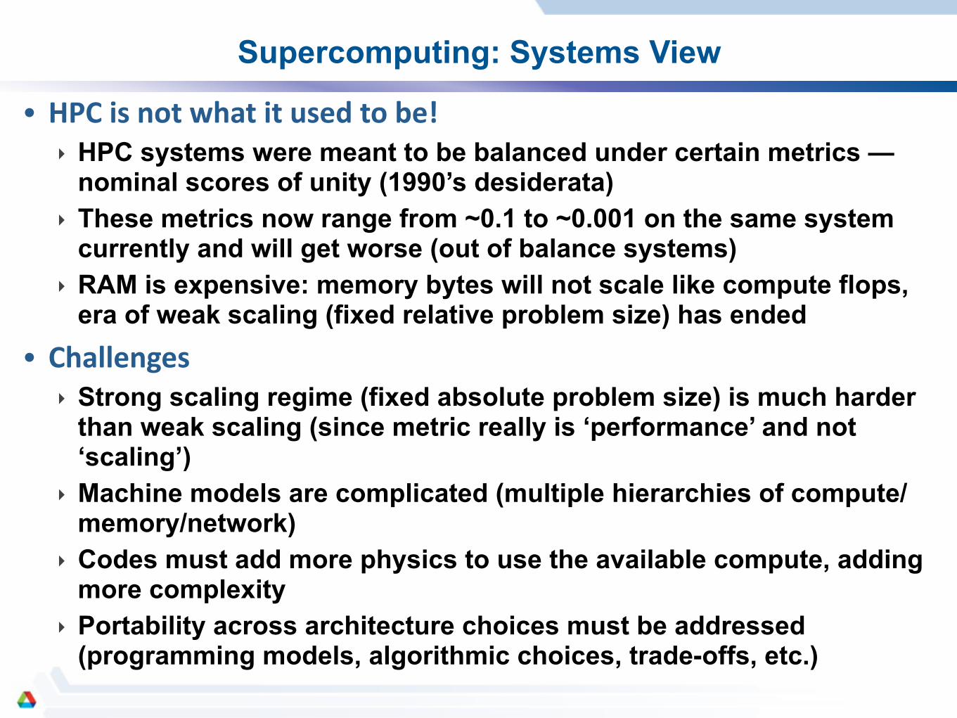
Supercomputing: Systems View
• HPC is not what it used to be! ‣ HPC systems were meant to be balanced under certain metrics —
nominal scores of unity (1990’s desiderata) ‣ These metrics now range from ~0.1 to ~0.001 on the same system
currently and will get worse (out of balance systems) ‣ RAM is expensive: memory bytes will not scale like compute flops,
era of weak scaling (fixed relative problem size) has ended • Challenges
‣ Strong scaling regime (fixed absolute problem size) is much harder than weak scaling (since metric really is ‘performance’ and not ‘scaling’)
‣ Machine models are complicated (multiple hierarchies of compute/memory/network)
‣ Codes must add more physics to use the available compute, adding more complexity
‣ Portability across architecture choices must be addressed (programming models, algorithmic choices, trade-offs, etc.)
Supercomputing Challenges: Sociological View
• Codes and Teams ‣ Most codes are written and maintained by small teams working
near the limits of their capability (no free cycles) ‣ Community codes, by definition, are associated with large inertia
(not easy to change standards, untangle lower-level pieces of code from higher-level organization, find the people required that have the expertise, etc.)
‣ Lack of consistent programming model for “scale-up” ‣ In some fields at least, something like a “crisis” is approaching (or
so people say) • What to do?
‣ We will get beyond this (the vector to MPP transition was worse) ‣ Transition needs to be staged (not enough manpower to entirely
rewrite code base) ‣ Prediction: There will be no ready made solutions ‣ Realization — “You have got to do it for yourself”
Co-Design vs. Code Design
• HPC Myths ‣ The magic compiler ‣ The magic programming model/language ‣ Special-purpose hardware ‣ Co-Design (not now anyway, but maybe in
the future —) • Dealing with Today’s Reality
‣ Code teams must understand all levels of the system architecture, but not be enslaved by it (software cycles are long)!
‣ Must have a good idea of the ‘boundary conditions’ (what may be available, what is doable, etc.)
‣ ‘Code Ports’ is ultimately a false notion ‣ Start thinking out of the box — domain
scientists and computer scientists and engineers must work together
Future heterogeneous manycore system, Borkar and Chien (2011)
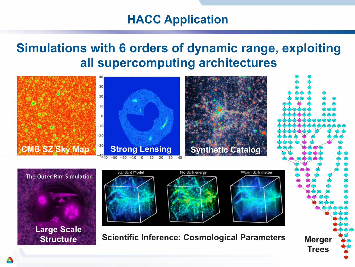
HACC Application
Simulations with 6 orders of dynamic range, exploiting all supercomputing architectures
The Outer Rim Simulation
CMB SZ Sky Map Strong Lensing Synthetic Catalog
Large Scale Structure Scientific Inference: Cosmological Parameters Merger
Trees
Large Scale Structure: Vlasov-Poisson Equation
Cosmological Vlasov-Poisson
Equation
• Properties of the Cosmological Vlasov-Poisson Equation: • 6-D PDE with long-range interactions, no shielding, all scales
matter; models gravity-only, collisionless evolution • Jeans instability drives structure formation at all scales from
smooth Gaussian random field initial conditions • Extreme dynamic range in space and mass (in many applications,
million to one in both space and density, ‘everywhere’) !
Large Scale Structure Simulation Requirements
• Force and Mass Resolution: • Galaxy halos ~100kpc, hence force
resolution has to be ~kpc; with Gpc box-sizes, a dynamic range of a million to one
• Ratio of largest object mass to lightest is ~10000:1
• Physics: • Gravity dominates at scales greater
than ~Mpc • Small scales: galaxy modeling, semi-
analytic methods to incorporate gas physics/feedback/star formation
• Computing ‘Boundary Conditions’: • Total memory in the PB+ class • Performance in the 10 PFlops+ class
• Wall-clock of ~days/week, in situ analysis
Can the Universe be run as a short computational
‘experiment’?
1000 Mpc
100 Mpc
20 Mpc
2 Mpc
Tim
e
Gravitational Jeans Instablity
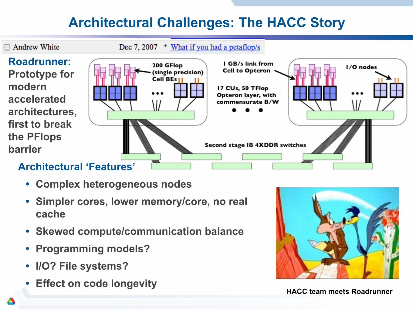
Architectural Challenges: The HACC Story
Mira/Sequoia
Roadrunner: Prototype for modern accelerated architectures, first to break the PFlops barrier
Architectural ‘Features’ • Complex heterogeneous nodes • Simpler cores, lower memory/core, no real
• Architecture-independent performance/scalability: ‘Universal’ top layer + ‘plug in’ node-level components; minimize data structure complexity and data motion
• Programming model: ‘C++/MPI + X’ where X = OpenMP, Cell SDK, OpenCL, CUDA, --
• Algorithm Co-Design: Multiple algorithm options, stresses accuracy, low memory overhead, no external libraries in simulation path
• Analysis tools: Major analysis framework, tools deployed in stand-alone and in situ modes
Roadrunner
Hopper
Mira/Sequoia
Titan
Edison
0.995
0.996
0.997
0.998
0.999
1
1.001
1.002
1.003
1.004
1.005
0.1 1
P(k) Ra
tio with r
espect
to GPU
code
k[h/Mpc]
RCB TreePM on BG/Q/GPU P3MRCB TreePM on Hopper/GPU P3M
Cell P3M/GPU P3MGadget-2/GPU P3M
1.00
1.003
0.997
Power spectra ratios across different implementations (GPU version as reference)
k (h/Mpc)
HACC Structure: Universal vs. Local Layers
Mira/Sequoia
Newtonian Force
Noisy CIC PM Force
6th-Order sinc-Gaussian spectrally filtered PM
ForceTw
o-pa
rtic
le F
orce
HACC Top Layer: 3-D domain decomposition with particle replication at boundaries (‘overloading’) for Spectral PM algorithm
(long-range force)
HACC ‘Nodal’ Layer: Short-range solvers
employing combination of flexible chaining mesh and RCB tree-based force
evaluations
RCB tree levels
~50 Mpc ~1 Mpc
Host-side: Scaling controlled by FFT
Performance controlled by short-range solver
HACC: Algorithmic Features and Options
• Fully Spectral Particle-Mesh Solver: 6th-order Green function, 4th-order Super-Lanczos derivatives, high-order spectral filtering, high-accuracy polynomial for short-range forces
• Custom Parallel FFT: Pencil-decomposed, high-performance FFT (up to 15K^3) • Particle Overloading: Particle replication at ‘node’ boundaries to reduce/delay
communication (intermittent refreshes), important for accelerated systems • Flexible Chaining Mesh: Used to optimize tree and P3M methods • Optimal Splitting of Gravitational Forces: Spectral Particle-Mesh melded with
direct and RCB (‘fat leaf’) tree force solvers (PPTPM), short hand-over scale (dynamic range splitting ~ 10,000 X 100); pseudo-particle method for multipole expansions
• Mixed Precision: Optimize memory and performance (GPU-friendly!) • Optimized Force Kernels: High performance without assembly • Adaptive Symplectic Time-Stepping: Symplectic sub-cycling of short-range
force timesteps; adaptivity from automatic density estimate via RCB tree • Custom Parallel I/O: Topology aware parallel I/O with lossless compression
(factor of 2); 1.5 trillion particle checkpoint in 4 minutes at ~160GB/sec on Mira
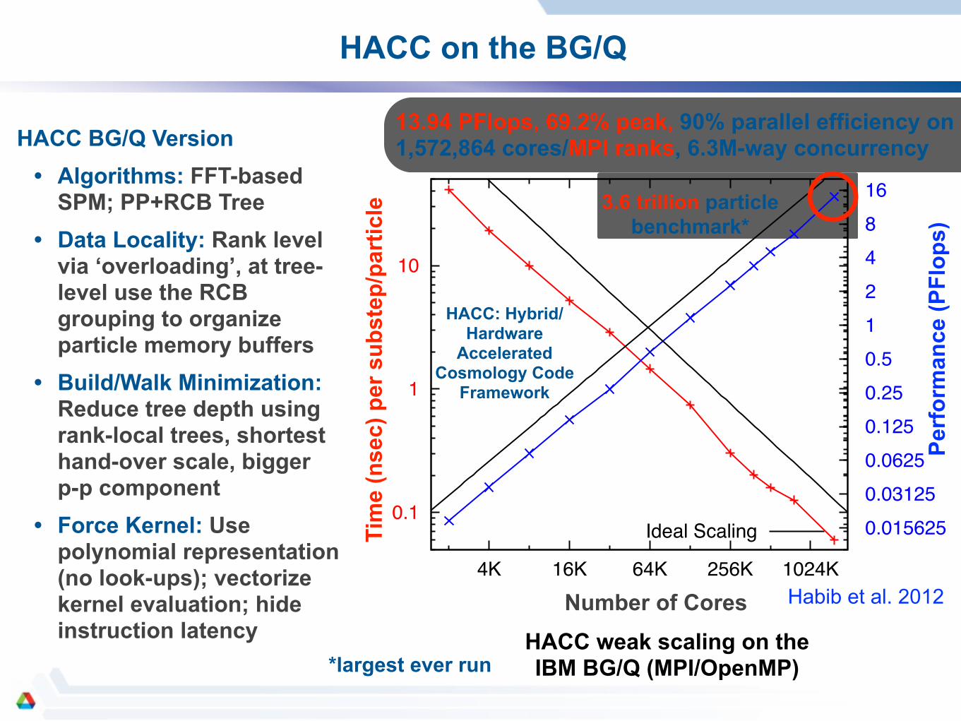
via ‘overloading’, at tree-level use the RCB grouping to organize particle memory buffers
• Build/Walk Minimization: Reduce tree depth using rank-local trees, shortest hand-over scale, bigger p-p component
• Force Kernel: Use polynomial representation (no look-ups); vectorize kernel evaluation; hide instruction latency
! *largest ever run
Accelerated Systems: HACC on Titan (Cray XK7)
Mira/Sequoia
Imbalances and Bottlenecks • Memory is primarily host-side
(32 GB vs. 6 GB) (against Roadrunner’s 16 GB vs. 16 GB), important thing to think about (in case of HACC, the ‘grid/particle’ balance)
• PCIe is a key bottleneck; overall interconnect B/W does not match Flops (not even close)
• There’s no point in ‘sharing’ work between the CPU and the GPU, performance gains will be minimal — GPU must dominate
• The only reason to write a code for such a system is if you can truly exploit its power (2 X CPU is a waste of effort!)
Strategies for Success • It’s (still) all about understanding
and controlling data motion • Rethink your code and even
approach to the problem • Isolate hotspots, and design for
portability around them (modular programming)
• Pragmas will never be the full answer (with maybe an exception or two)
HACC on Titan: GPU Implementation (Schematic)
Block3 Grid units
Push to GPU
Chaining Mesh
P3M Implementation (OpenCL): • Spatial data pushed to GPU in
large blocks, data is sub-partitioned into chaining mesh cubes
• Compute forces between particles in a cube and neighboring cubes
• Natural parallelism and simplicity leads to high performance
• Typical push size ~2GB; large push size ensures computation time exceeds memory transfer latency by a large factor
• More MPI tasks/node preferred over threaded single MPI tasks (better host code performance)
New Implementations (OpenCL and CUDA):
• P3M with data pushed only once per long time-step, completely eliminating memory transfer latencies (orders of magnitude less); uses ‘soft boundary’ chaining mesh, rather than rebuilding every sub-cycle
• TreePM analog of BG/Q code written in CUDA, also produces high performance
HACC on Titan: GPU Implementation Performance
• P3M kernel runs at
1.6TFlops/node at 40.3% of peak (73% of algorithmic peak)
• TreePM kernel was run on 77% of Titan at 20.54 PFlops at almost identical performance on the card
• Because of less overhead, P3M code is (currently) faster by factor of two in time to solution
!
Ideal Scaling
Initial Strong ScalingInitial Weak Scaling
Improved Weak Scaling
TreePM Weak Scaling
Tim
e (n
sec)
per
sub
step
/par
ticle
Number of Nodes
99.2% Parallel Efficiency
Summary
Basic Ideas: • Thoughtful design of flexible code infrastructure; minimize number of
• Because machines are so out of balance, focusing only on the lowest-level compute-intensive kernels can be a mistake (‘code ports’)
• One possible solution is an overarching universal layer with architecture-dependent, plug-in modules (with implications for productivity)
• Understand data motion issues in depth — minimize data motion, always look to hide communication latency with computation
• Be able to change on fast timescales (HACC needs no external libraries in the main simulation code — helps to get on new machines early)
• As science outputs become more complex, data analysis becomes a very significant fraction of available computational time — optimize performance with this in mind
EXTRA SLIDES
Separation of Scales (cont.)
The problem: What are flong
(r1� r2) and fshort
(r1� r2)?
The answer: flong
(r1� r2), the “grid softened force”, can be determinedempirically. The force computed by the particle-mesh technique is sampledfor many particle separations, and the resulting samples are fit by apolynomial. f
short
(r1� r2) is then trivially determined by subtraction.
The question: How to best compute fshort
(r1� r2).
The answer: This depends on the architecture!
Hal Finkel (Argonne National Laboratory) HACC Performance July 31, 2013 3 / 19
Force Splitting
The gravitational force calculation is split into long-range part and ashort-range part
A grid grid is responsible for largest 4 orders of magnitude of dynamicrange
particle methods handle the critical 2 orders of magnitude at theshortest scales
Complexity:
PM (grid) algorithm: O(Np
)+O(Ng
log Ng
), where Np
is the totalnumber of particles, and N
g
the total number of grid points
tree algorithm: O(Npl
log Npl
), where Npl
is the number of particlesin individual spatial domains (N
pl
⌧ Np
)
the close-range force computations are O(N2
d
) where Nd
is thenumber of particles in a tree leaf node within which all directinteractions are summed
Hal Finkel (Argonne National Laboratory) HACC Performance July 31, 2013 5 / 19
Force Splitting (cont.)
Long-Range Algorithm:
The long/medium range algorithm is based on a fast, spectrallyfiltered PM method
The density field is generated from the particles using a Cloud-In-Cell(CIC) scheme
The density field is smoothed with the (isotropizing) spectral filter:
exp (�k2�2/4) [(2k/�) sin(k�/2)]ns , (1)
where the nominal choices are � = 0.8 and ns
= 3. The noise reductionfrom this filter allows matching the short and longer-range forces at aspacing of 3 grid cells.
The Poisson solver uses a sixth-order, periodic, influence function(spectral representation of the inverse Laplacian)
The gradient of the scalar potential is obtained using higher-orderspectral di↵erencing (fourth-order Super-Lanczos)
Hal Finkel (Argonne National Laboratory) HACC Performance July 31, 2013 6 / 19
Force Splitting (cont.)
The “Poisson-solve” is the composition of all the kernels above in onesingle Fourier transform
Each component of the potential field gradient then requires anindependent FFT
Distributed FFTs use a pencil decomposition
To obtain the short-range force, the filtered grid force is subtractedfrom the Newtonian force
Mixed precision:
single precision is adequate for the short/close-range particle forceevaluations and particle time-stepping
double precision is used for the spectral component
Hal Finkel (Argonne National Laboratory) HACC Performance July 31, 2013 7 / 19
Overloading
The spatial domain decomposition is in regular 3-D blocks, but unlike theguard zones of a typical PM method, full particle replication – termed‘particle overloading’ – is employed across domain boundaries.
Hal Finkel (Argonne National Laboratory) HACC Performance July 31, 2013 8 / 19
Overloading (cont.)
Works because particles cluster and large-scale bulk motion is small
Short-range force contribution is not used for particles near the edgeof the overloading region
The typical memory overhead cost for a large run is ⇠ 10%
The point of overloading is to allow su�ciently-exactmedium/long-range force calculations with no communication ofparticle information and high-accuracy local force calculations
We use relatively sparse refreshes of the overloading zone! This is key tofreeing the overall code performance from the weaknesses of theunderlying communications infrastructure.
Hal Finkel (Argonne National Laboratory) HACC Performance July 31, 2013 9 / 19
Time Stepping
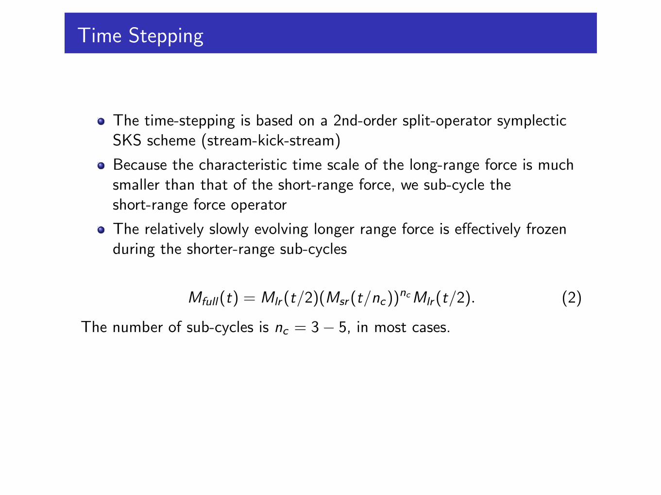
The time-stepping is based on a 2nd-order split-operator symplecticSKS scheme (stream-kick-stream)
Because the characteristic time scale of the long-range force is muchsmaller than that of the short-range force, we sub-cycle theshort-range force operator
The relatively slowly evolving longer range force is e↵ectively frozenduring the shorter-range sub-cycles
Mfull
(t) = Mlr
(t/2)(Msr
(t/nc
))nc Mlr
(t/2). (2)
The number of sub-cycles is nc
= 3� 5, in most cases.
Hal Finkel (Argonne National Laboratory) HACC Performance July 31, 2013 10 / 19
RCB Tree
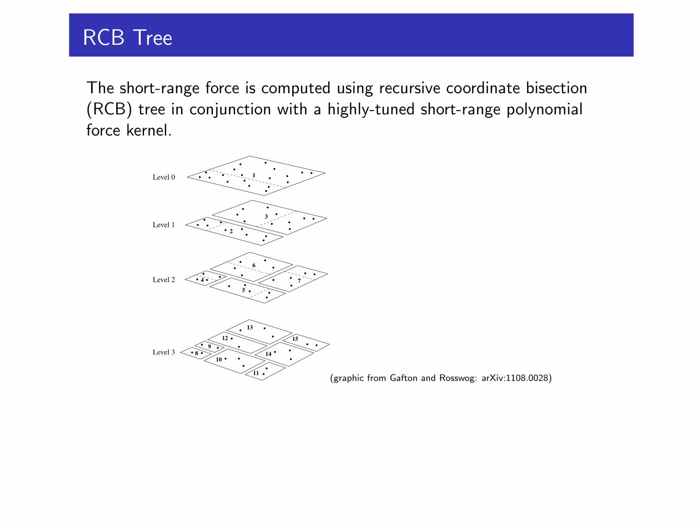
The short-range force is computed using recursive coordinate bisection(RCB) tree in conjunction with a highly-tuned short-range polynomialforce kernel.
Level 0
Level 1
Level 2
Level 3
1
2
3
45
6
7
89
10
11
12
13
14
15
(graphic from Gafton and Rosswog: arXiv:1108.0028)
Hal Finkel (Argonne National Laboratory) HACC Performance July 31, 2013 11 / 19
RCB Tree (cont.)
At each level, the node is split at its center of mass
During each node split, the particles are partitioned into disjointadjacent memory bu↵ers
This partitioning ensures a high degree of cache locality during theremainder of the build and during the force evaluation
To limit the depth of the tree, each leaf node holds more than oneparticle. This makes the build faster, but more importantly, tradestime in a slow procedure (a “pointer-chasing” tree walk) for a fastprocedure (the polynomial force kernel).
Hal Finkel (Argonne National Laboratory) HACC Performance July 31, 2013 12 / 19
Force Kernel
Due to the compactness of the short-range interaction, the kernel can berepresented as
fSR
(s) = (s + ✏)�3/2 � fgrid
(s) (3)
where s = r · r, fgrid
(s) = poly[5](s), and ✏ is a short-distance cuto↵.
An interaction list is constructed during the tree walk for each leafnode
When using fine-grained threading: using OpenMP, the particles inthe leaf node are assigned to di↵erent threads: all threads share theinteraction list (which automatically balances the computation)
The interaction list is processed using a vectorized kernel routine(written using QPX/SSE compiler intrinsics)
Filtering for self and out-of-range interactions uses the floating-pointselect instruction: no branching required
We can use the reciprocal (sqrt) estimate instructions: no library calls
Hal Finkel (Argonne National Laboratory) HACC Performance July 31, 2013 14 / 19