Extreme_Risk_Analysis_JPM_Spring_2010

The Journal of Performance MeasurementSpring 2010 -17-

Extreme Risk Analysis

Risk analysis involves gaining deeper insight into the sources of risk and evaluating whether these risks accurate-ly reflect the views of the portfolio manager. In this paper we show how to extend standard volatility analytics toshortfall, a measure of extreme risk. Using two examples, we show how shortfall provides a more complete andintuitive picture of risk than value at risk. In two subsequent examples we illustrate the additional perspectiveoffered by analyzing shortfall and volatility in tandem.

Lisa Goldberg, Ph.D.

is Executive Director and Global Head of Risk Analytics at MSCI and Adjunct Professor of Statistics at UCBerkeley. Prior to joining MSCI in 1993, Dr. Goldberg was a Professor of Mathematics at UC Berkeley and CityUniversity of New York, and she has held positions at The Institute for Advanced Study, Institut des Hautes ÉtudesScientifiques and The Mathematical Sciences Research Institute. Dr. Goldberg received a Ph.D. in Mathematicsfrom Brandeis University in 1984 and has received numerous academic awards including the prestigious SloanFellowship. Dr. Goldberg’s current professional focus is the design and implementation of extreme risk manage-ment paradigms that are useful to financial practitioners and regulators. Her research interests include riskmeasurement and analysis, statistical assessment of financial forecasts, credit models, index construction andgreen investing. Dr. Goldberg is the primary architect of MSCI’s extreme risk and credit models and she has beenawarded three patents. Dr. Goldberg publishes and lectures extensively in both financial economics and mathe-matics. She serves on the board of the JOIM Conference series and the editorial board of two Springer bookseries, and as a moderator for arXiv Quantitative Finance. She is co-author of “Portfolio Risk Analysis,” pub-lished in 2010 in the Princeton University Press Finance Series.

Jose Menchero, Ph.D., CFA

is Executive Director and Global Head of Equity Factor Model Research at MSCI. Dr. Menchero manages aninternational team of researchers and is responsible for the continuous development and improvement of all equi-ty factor risk models and the Barra Integrated Model. He and his team also develop portfolio analytics for returnand risk attribution. Before joining MSCI, Jose was Head of Quantitative Research at Thomson Financial, wherehe worked on performance attribution, risk attribution, and factor risk modeling. Dr. Menchero has several pub-lications in these areas. Prior to entering finance, Dr. Menchero was a Professor of Physics at the University ofRio de Janeiro, Brazil. His area of research was in the Quantum Theory of Solids, and he also has several pub-lications in this field. Jose serves on the Advisory Board of The Journal of Performance Measurement. He holdsa B.Sc. in Aerospace Engineering from the University of Colorado at Boulder, and a Ph.D. in Theoretical Physicsfrom the University of California at Berkeley.

Michael Hayes, Ph.D.

is a Senior Associate at MSCI, and a principal architect of Barra Extreme Risk and Power VaR. He is currentlyfocusing on how to incorporate extreme risk into portfolio construction, and is developing a new paradigm forempirical stress testing and scenario analysis using Barra factors. Dr. Hayes earned his Ph.D. in ChemicalPhysics from the University of Colorado, and his B.A. from Princeton University. He has authored more than adozen research papers in the fields of chemistry, physics, and finance.

Indrajit Mitra, Ph.D.

is currently a graduate student at MIT, where he is pursuing a Ph.D. in Finance. Prior to attending MIT, Indrajitworked as a senior quantitative analyst at MSCI, where he focused on factor modeling, extreme risk, and portfo-lio analytics. Indrajit has a Ph.D. in theoretical physics from Princeton University.

The Journal of Performance Measurement -18- Spring 2010

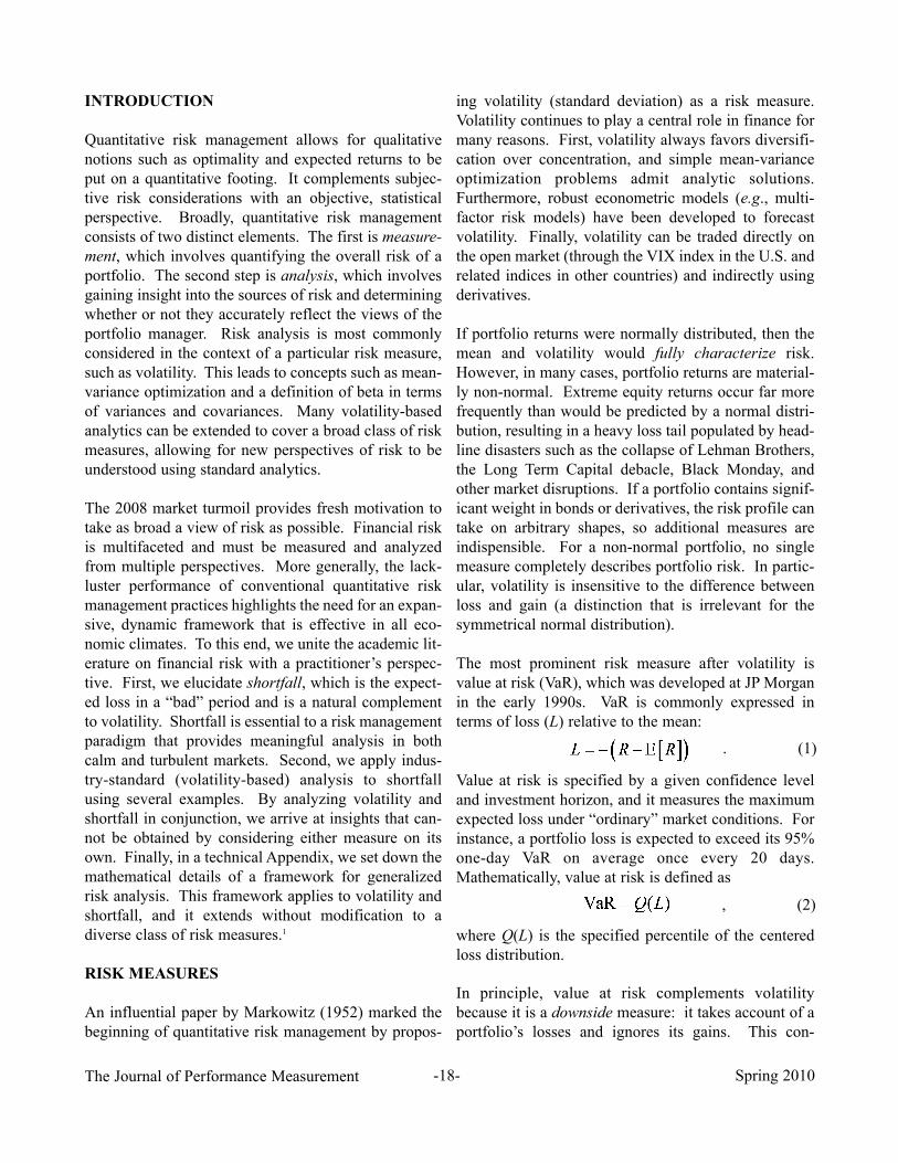
IntRoDuCtIon

Quantitative risk management allows for qualitative

notions such as optimality and expected returns to be

put on a quantitative footing. It complements subjec-

tive risk considerations with an objective, statistical

perspective. Broadly, quantitative risk management

consists of two distinct elements. The first is measure-ment, which involves quantifying the overall risk of a

portfolio. The second step is analysis, which involves

gaining insight into the sources of risk and determining

whether or not they accurately reflect the views of the

portfolio manager. Risk analysis is most commonly

considered in the context of a particular risk measure,

such as volatility. This leads to concepts such as mean-

variance optimization and a definition of beta in terms

of variances and covariances. Many volatility-based

analytics can be extended to cover a broad class of risk

measures, allowing for new perspectives of risk to be

understood using standard analytics.

The 2008 market turmoil provides fresh motivation to

take as broad a view of risk as possible. Financial risk

is multifaceted and must be measured and analyzed

from multiple perspectives. More generally, the lack-

luster performance of conventional quantitative risk

management practices highlights the need for an expan-

sive, dynamic framework that is effective in all eco-

nomic climates. To this end, we unite the academic lit-

erature on financial risk with a practitioner’s perspec-

tive. First, we elucidate shortfall, which is the expect-

ed loss in a “bad” period and is a natural complement

to volatility. Shortfall is essential to a risk management

paradigm that provides meaningful analysis in both

calm and turbulent markets. Second, we apply indus-

try-standard (volatility-based) analysis to shortfall

using several examples. By analyzing volatility and

shortfall in conjunction, we arrive at insights that can-

not be obtained by considering either measure on its

own. Finally, in a technical Appendix, we set down the

mathematical details of a framework for generalized

risk analysis. This framework applies to volatility and

shortfall, and it extends without modification to a

diverse class of risk measures.1

RIsk MEAsuREs

An influential paper by Markowitz (1952) marked the

beginning of quantitative risk management by propos-

ing volatility (standard deviation) as a risk measure.

Volatility continues to play a central role in finance for

many reasons. First, volatility always favors diversifi-

cation over concentration, and simple mean-variance

optimization problems admit analytic solutions.

Furthermore, robust econometric models (e.g., multi-

factor risk models) have been developed to forecast

volatility. Finally, volatility can be traded directly on

the open market (through the VIX index in the U.S. and

related indices in other countries) and indirectly using

derivatives.

If portfolio returns were normally distributed, then the

mean and volatility would fully characterize risk.

However, in many cases, portfolio returns are material-

ly non-normal. Extreme equity returns occur far more

frequently than would be predicted by a normal distri-

bution, resulting in a heavy loss tail populated by head-

line disasters such as the collapse of Lehman Brothers,

the Long Term Capital debacle, Black Monday, and

other market disruptions. If a portfolio contains signif-

icant weight in bonds or derivatives, the risk profile can

take on arbitrary shapes, so additional measures are

indispensible. For a non-normal portfolio, no single

measure completely describes portfolio risk. In partic-

ular, volatility is insensitive to the difference between

loss and gain (a distinction that is irrelevant for the

symmetrical normal distribution).

The most prominent risk measure after volatility is

value at risk (VaR), which was developed at JP Morgan

in the early 1990s. VaR is commonly expressed in

terms of loss (L) relative to the mean:

Value at risk is specified by a given confidence level

and investment horizon, and it measures the maximum

expected loss under “ordinary” market conditions. For

instance, a portfolio loss is expected to exceed its 95%

one-day VaR on average once every 20 days.

Mathematically, value at risk is defined as

where Q(L) is the specified percentile of the centered

loss distribution.

In principle, value at risk complements volatility

because it is a downside measure: it takes account of a

portfolio’s losses and ignores its gains. This con-

. (1)

, (2)


tributed to the inclusion of VaR in the Basel II regula-

tory framework. However, certain drawbacks of VaR

are well appreciated (The Economist, 2004). Some of

these drawbacks relate to the way in which VaR is esti-

mated or interpreted. Even if those are addressed,

problems remain in the very definition of VaR.

A significant shortcoming of VaR is that – unlike

volatility – it may actually encourage concentrationover diversification. That is, lowering VaR may some-

times lead to a more concentrated portfolio. A schemat-

ic example shows how this can happen.2

Example 1: Value at Risk and Diversification

Consider investing in two corporate bonds that are con-

tractually identical; the only difference between the

bonds is that they are issued by different firms. Is it

better to invest in one of the bonds or to diversify with

some of each? Suppose that the annual default proba-

bility of both issuers is 0.7 percent. This means that

each firm has just under a one-in-a-hundred chance of

defaulting over the next twelve months. Defaults are

improbable events, and value at risk does not raise any

concern: hold only one of the two bonds and your 99%

VaR (considering only default risk) is zero. This is

because VaR is a worst-case scenario for an ordinary

year. In any one of the 99 tamer years in a typical hun-

dred, the issuer does not default, and investment in

either bond pays dividends.

How risky is it to put half the money in each of the two

bonds? Assuming the defaults are independent, the

probability that something goes wrong approximately

doubles to 1.4 percent. As a result, the 99% value at

risk increases to little less than half the principal. In

other words, diversification raises value at risk from

zero to almost half the portfolio value. What went

wrong? Value at risk punishes the two-bond portfolio

for a greater probability of an adverse event. However,

it is relatively insensitive to the event’s magnitude. The

magnitudes of the adverse events differ (materially) by

a factor of two. A single-bond portfolio loses its entire

principal, while the two-bond portfolio loses at least

half, but usually no more than half, of its principal.

As an upper bound for loss on an ordinary day, VaR is

also a lower bound for loss on an extraordinary day. Itgives no indication of what to expect on an extraordi-

nary day. While it is a measure of downside risk, VaR

is not a measure of extreme risk. Are typical breaches

of a VaR limit mild infractions or egregious violations?

This question is beyond the scope of VaR; it can be

answered only by a true measure of extreme risk.

Shortfall (S) is a natural extension of value at risk and

is a true extreme risk measure. It is the expected port-

folio loss given that VaR has been breached:

In other words, shortfall is an estimate of what to expect

in a “bad” period. It is impossible to hide tail risk from

shortfall the way it can be hidden with VaR. In

Example 1, shortfall favors the two-bond portfolio over

a single-bond portfolio. More generally shortfall, like

volatility but unlike VaR, will always encourage diver-

sification. Next, we investigate the difference between

VaR and shortfall using a set of portfolios that are long

an ETF and short call options on the ETF.

Example 2: The Risk of a Short Position in Call

Options

Out-of-the-money call options are commonly sold to

enhance portfolio returns. The option issuer receives a

premium when the option is written. Under ordinary

market conditions, the underlying security experiences,

at best, a modest gain, and the option expires out of the

money. However, an extreme gain to the underlying

can trigger a devastating loss to the issuer of the option.

Using an empirically realistic (non-normal) distribution

for the portfolio, we show that shortfall is a better gauge

of the risk of the short position than VaR.

Consider a family of portfolios, each composed of a

single share of an exchange traded fund (ETF) and a

short position in a variable number of identical

European call options. The underlying chosen is the

MSCI U.S. Broad Market Index,3 and the analysis date

is October 23, 2008. The spot price of the index is

taken as $60, and the strike price of each option is $64,

with one day to expiration.

If the short position consists of more than one option,

the portfolio has an infinite down side – the potential to

lose an arbitrarily large amount of money – since there

is no upper limit to the value of the ETF. What is the

one-day risk of holding such a portfolio? The risk of

. (3)


Figure 1:

One-day shortfall and Value at Risk, at 95% confidence level, plotted versus number

of options in the portfolio. The portfolio is long an ETF, and short a variable num-

ber of out-of-the-money call options.

this family of portfolios as viewed through the lens of

VaR and shortfall is illustrated in Figure 1. As the plot

clearly shows, VaR does not significantly increase with

the number of call options sold, while shortfall increas-

es roughly linearly with the number of short positions.

The portfolio loses value from two types of scenarios:

(a) the ETF experiences a moderate loss, in excess of

the call premiums, and (b) the ETF experiences a large

gain, so the call options are exercised. Losses of the

first kind are largely insensitive to the number of calls

sold.4 By contrast, losses resulting from the calls being

exercised increase in direct proportion to the number of

calls written.

If the call option is sufficiently deep out of the money

(i.e., the strike price is sufficiently higher than the spot

price) most of the losses are from the ETF losing value.

In particular, the smallest of the large losses are of this

kind. This implies that for such a portfolio, VaR would

be quite insensitive to the number of short positions.

More importantly, it disregards the impact of large loss-

es resulting from scenarios (b). Shortfall, on the other

hand, averages over all large losses including scenarios

of the second kind, for which a portfolio short 10 call

options will lose 10 times as much as a portfolio short

a single call option.

RIsk AnALysIs

Once risk has been measured, the next step is to under-

stand the sources of risk and how they interact.

Different investors may be interested in different types

of sources, such as individual securities, asset classes,

sectors, industries, currencies, or style factors from a

particular risk model. Portfolio risk can be analyzed in

terms of any type of source, so we make our discussion

generic by considering sources without reference to

their type.

RIsk souRCEs

Fix an investment period and let rm denote the return to

source m over this period. Then the portfolio return

over the period is given by a sum,

, (4)

20

16

18

14

12

10

8

6

40 1 2 3 4 5 6 7 8 9 10

Ris

k (

Per

cent)

Number of Options

Shortfall

VaR


where xm is the portfolio exposure to the source m. It is

the job of the portfolio manager to determine the source

exposures at the start of a period. The source returns

are random variables, whose realized values are known

only at the end of the investment period.

RIsk ContRIbutIons

Portfolio risk is not a weighted sum of source risks, so

there is no direct analog to Equation 4 for risk.

However, there is a parallel to Equation 4 in terms of

marginal contributions to risk (MCR). The marginal

contribution to risk of a source m is the approximate

change in portfolio risk when increasing the source

exposure by a small amount , while keeping all

other exposures fixed,

The contribution of a return source to portfolio risk is

given precisely by the product of the source exposure

and the marginal contribution to risk, as shown by

Litterman (1996) in the context of volatility , and

these risk contributions sum to the portfolio risk:

In the Appendix, we show that Equation 6 holds for a

large class of risk measures including shortfall, and it

facilitates meaningful, even-handed decompositions of

different risk measures.

X-Sigma-Rho Risk Attribution

Additional insight can be provided by a refinement of

the Litterman (1996) decomposition for volatility given

in Equation 6. As discussed in Menchero and Poduri

(2008), the marginal contribution to volatility can be

expressed as the product of the stand-alone volatility of

the source and the correlation of the source return with

the portfolio,

This gives rise to the x-sigma-rho risk attribution for-

mula,

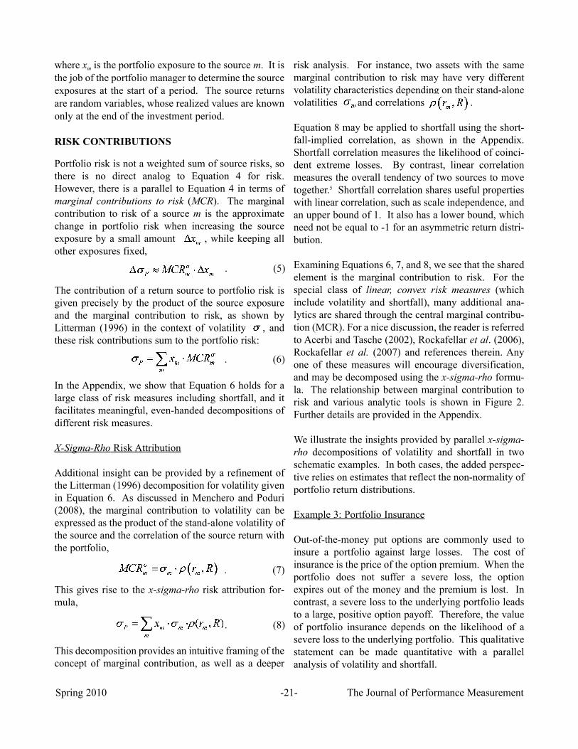
This decomposition provides an intuitive framing of the

concept of marginal contribution, as well as a deeper

risk analysis. For instance, two assets with the same

marginal contribution to risk may have very different

volatility characteristics depending on their stand-alone

volatilities and correlations .

Equation 8 may be applied to shortfall using the short-

fall-implied correlation, as shown in the Appendix.

Shortfall correlation measures the likelihood of coinci-

dent extreme losses. By contrast, linear correlation

measures the overall tendency of two sources to move

together.5 Shortfall correlation shares useful properties

with linear correlation, such as scale independence, and

an upper bound of 1. It also has a lower bound, which

need not be equal to -1 for an asymmetric return distri-

bution.

Examining Equations 6, 7, and 8, we see that the shared

element is the marginal contribution to risk. For the

special class of linear, convex risk measures (which

include volatility and shortfall), many additional ana-

lytics are shared through the central marginal contribu-

tion (MCR). For a nice discussion, the reader is referred

to Acerbi and Tasche (2002), Rockafellar et al. (2006),

Rockafellar et al. (2007) and references therein. Any

one of these measures will encourage diversification,

and may be decomposed using the x-sigma-rho formu-

la. The relationship between marginal contribution to

risk and various analytic tools is shown in Figure 2.

Further details are provided in the Appendix.

We illustrate the insights provided by parallel x-sigma-rho decompositions of volatility and shortfall in two

schematic examples. In both cases, the added perspec-

tive relies on estimates that reflect the non-normality of

portfolio return distributions.

Example 3: Portfolio Insurance

Out-of-the-money put options are commonly used to

insure a portfolio against large losses. The cost of

insurance is the price of the option premium. When the

portfolio does not suffer a severe loss, the option

expires out of the money and the premium is lost. In

contrast, a severe loss to the underlying portfolio leads

to a large, positive option payoff. Therefore, the value

of portfolio insurance depends on the likelihood of a

severe loss to the underlying portfolio. This qualitative

statement can be made quantitative with a parallel

analysis of volatility and shortfall.

. (5)

. (6)

. (7)

. (8)


Figure 2:

Schematic diagram showing relationships between marginal contribution to risk and

other widely used measures. Here, denotes a generalized risk measure.

An investor seeks to measure the reduction of risk

when insuring an ETF on the MSCI US Broad Market

Index with an out-of-the-money put option on the same

index. The spot price of the index is $60 and the option

strike is $50. The analysis date is October 23, 2008,

with the option expiration at 20 days.6 We analyze port-

folio risk in terms of both volatility and shortfall.

Volatility paints an incomplete picture of this risk due

to the non-normality of the return distribution of the

portfolio.7 Since a larger loss from the index generates

greater option profits, the diversification benefit of

holding put options increases as the risk measure

becomes more concentrated in the tail of the portfolio

distribution. We consider the risk of the portfolio as the

option weight is varied. In Figure 3, we plot the contri-

butions to 99% shortfall from the option and the index.

Initially, the option strongly reduces the risk of the port-

folio. The portfolio risk is minimized for an option

weight of about 7 percent. Eventually, however,

increasing the option weight becomes more of a gamble

on a market crash, thus increasing the portfolio risk.

In Figure 4, we show the contributions of the option and

the index to portfolio volatility as the option weight is

varied. Qualitatively, the results are similar to Figure 3,

with the portfolio risk first declining and then increas-


Figure 3:

Contribution to 99% shortfall from index and option, as option

weight is varied. The fully hedged option weight is indicated by

the vertical dashed line. The minimum risk portfolio occurs for an

option weight of about 7 percent.

Figure 4:

Contribution to volatility from index and option, plotted as

option weights are varied. The fully hedged option weight is

indicated by the vertical dashed line.

15

10

5

0

-5

-10

0 2 4 6 8 10 12 14

99%

Short

fall

Contr

ibuti

on

Option Weight (Percent)

10

8

6

4

2

0

-2

-40 2 4 6 8 10 12 14

Vola

tili

ty C

ontr

ibuti

on (

per

cent)

Option Weight (Percent)

Index

Total

Option

OptionIndex

Total


ing as the option weight is varied. Note the relative

amount by which the risk is reduced: the put option is

much more effective at reducing 99% shortfall risk than

at reducing portfolio volatility.

In Table 1, we use the x-sigma-rho methodology to

decompose three risk measures: volatility, 95% short-

fall, and 99% shortfall. The horizon in all cases is taken

to be one day. The portfolio is fully hedged, meaning

that there are equal number of shares in the ETF and the

option. This results in an index weight of 98.86%, and

an option weight of 1.14%, as indicated in Column 1.

In the x-sigma-rho framework, the risk contribution is

given by the product of the exposure (x), the stand-

alone risk (sigma), and the generalized correlation

(rho). Note that the exposures are the same for all three

risk measures.

The option contributes -169 basis points to 95% short-

fall. Note that the shortfall correlation is -2.11. This

value is noteworthy since linear (volatility-implied)

correlation can never fall below -1. Shortfall correla-

tion, on the other hand, can be less than -1 due to the

asymmetry of the risk measure and return distribution.

As shown in the Appendix, the shortfall correlation

between the option loss and the portfolio loss L is

given by the ratio of two terms: (1) the expected option

loss (lm) on days when the portfolio VaR is breached,

and (2) the shortfall of the option.

The distribution of centered option losses is shown in

Figure 5. The right side of the distribution represents

the worst 5% of option scenarios, when the 95% option

VaR is breached. The left side of the distribution rep-

resents option losses on the worst 5% of portfolio sce-

narios, showing that the option performs well when the

portfolio suffers losses. The numerator of Equation

A17 is the mean of the leftside of the distribution, or

table 1:

Risk decomposition for volatility, 95% shortfall, and 99% shortfall, using the x-sigma-rho formulation.

The portfolio consists of an index and an out-of-the-money put option on the same index.

-148.6 percent. The denominator of Equation A17 is

the mean of the right side of the distribution, or 70.6%.

The correlation of -2.11 is the ratio of these two num-

bers.

In the final example, we examine a portfolio composed

of two assets that are uncorrelated by the standard

volatility measure, but that nevertheless tend to experi-

ence large coincident losses. This may be the result of

financial contagion, where an extreme move in one

asset triggers an extreme move in another. Standard

volatility and correlation measures are insensitive to the

risk of extreme coincident losses. However, this risk

can be measured using shortfall and shortfall-implied

correlation.

Example 4: Coincident Extreme Losses

We consider two portfolios, each composed of two

equally-weighted assets whose returns follow standard

normal distributions. The portfolios are distinguished

only by the joint distributions of the two assets. First,

we use a normal copula, which ensures that the joint

distribution is also normally distributed. Copulas pro-

vide a method of formulating multivariate return distri-

butions with given statistical properties (Nelsen, 1999).

The second way in which we form the joint distribution

is to use the t-copula, which exhibits a greater likeli-

hood of joint extreme losses. We stress that although

the asset returns generated by the t-copula are uncorre-

lated using the conventional definition, they are not

independent. Therefore, even though the asset returns

are normally distributed, the portfolio returns are fat

tailed due to the increased likelihood of both assets

experiencing extreme simultaneous losses.

To compute the risk of these portfolios, we take one

million random draws from the two bivariate distribu-


Figure 5:

Partial histogram of centered option losses, defined as the option loss relative to the mean option loss

. The theoretical maximum centered option loss is therefore 114.74%. The right side of the distribu-

tion is for bad option days, defined as days when the 95% option VaR (60.2%) is breached. The expected cen-

tered option loss on bad option days is 70.6%. The left side of the distribution is for days when the 95% port-

folio VaR is breached. The mean centered option loss on bad portfolio days is -148.6% (i.e., the option per-

forms well on bad portfolio days). The 95% shortfall correlation is the ratio of the two numbers, i.e., -2.11.

Note that the left side of the distribution has a long tail, and all losses

beyond -280% are trimmed for plotting purposes.

table 2:

X-sigma-rho risk decomposition for two identical assets assuming a normal copula.

tions. In Table 2, we perform an x-sigma-rho attribu-

tion of volatility and shortfall for the case of a normal

copula. Since the portfolio is equally weighted, the

exposure to each asset is 50 percent. Following the

standard computations for volatility, the correlation of

each asset with the portfolio is , or 0.71. The

portfolio volatility is 0.71%, compared to a stand-alone

volatility of 1% for each asset.

For 95% shortfall, the stand-alone risk of each asset is

2.06 percent. For normal distributions, the ratio of 95%

shortfall to volatility is 2.06. The shortfall correlation

is the same as the volatility correlation (i.e., 0.71). The

95% shortfall for the portfolio is 1.46, which is exactly

2.06 times the portfolio volatility. This is as expected,

since the portfolio returns are normally distributed.

More interesting is the risk decomposition for the t-cop-

ula, given in Table 3. Note that the volatility of the

portfolio is unchanged. The correlation of each asset

250

200

150

100

50

0-300 -250 -200 -150 -100 -50 0 50 100

Count

Excess Option Loss (percent)

Bad Option Days

Bad Portfolio Days


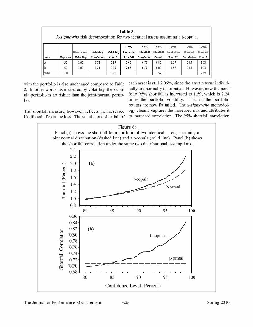
with the portfolio is also unchanged compared to Table

2. In other words, as measured by volatility, the t-cop-

ula portfolio is no riskier than the joint-normal portfo-

lio.

The shortfall measure, however, reflects the increased

likelihood of extreme loss. The stand-alone shortfall of

table 3:

X-sigma-rho risk decomposition for two identical assets assuming a t-copula.

Figure 6:

Panel (a) shows the shortfall for a portfolio of two identical assets, assuming a

joint normal distribution (dashed line) and a t-copula (solid line). Panel (b) shows

the shortfall correlation under the same two distributional assumptions.

each asset is still 2.06%, since the asset returns individ-

ually are normally distributed. However, now the port-

folio 95% shortfall is increased to 1.59, which is 2.24

times the portfolio volatility. That is, the portfolio

returns are now fat tailed. The x-sigma-rho methodol-

ogy cleanly captures the increased risk and attributes it

to increased correlation. The 95% shortfall correlation

2.4

2.2

2.0

1.8

1.6

1.4

1.2

1.0

0.8

80 85 90 95 100

Short

fall

(P

erce

nt) (a)

t-copula

Normal

(b)

t-copula

Normal

0.86

0.84

0.82

0.80

0.78

0.76

0.74

0.72

0.70

0.68

80 85 90 95 100

Short

fall

Corr

elat

ion

Confidence Level (Percent)


is 0.77, and increases to 0.85 as we move deeper with-

in the tail (i.e., 99% shortfall).

Figure 6 illustrates the effects of the joint distribution

on portfolio risk. In Figure 6(a), we plot portfolio

shortfall versus confidence level. As we move further

into the tail, the portfolio with returns following the t-copula appears riskier, due to the likelihood of coinci-

dent extreme losses. In Figure 6(b), we plot the short-

fall correlation versus confidence level. For the joint

normal distribution, shortfall correlation is 0.71 at all

confidence levels. For the t-copula portfolio, however,

the shortfall correlation increases with confidence

level, thus indicating the increased likelihood of large

coincident losses.

ConCLusIon

The extreme turbulence that plagued financial markets

in 2008 and 2009 highlights the importance of taking a

broad, dynamic view of risk. This means that investors

need to extend standard risk management practices to

include measures of extreme risk. Shortfall, which is

the expected loss given that the VaR threshold has been

breached, is the most important measure of extreme

risk. It probes the tails of portfolio return distributions,

promotes diversification, and is easily amenable to the

tools of standard risk analysis.

Parallel decompositions of portfolio volatility and

shortfall provide insights that cannot be obtained

through the lens of a single risk measure. We illustrate

two such insights in this article. The first is a deep

understanding of the value of downside protection: the

diversification benefits of an out-of-the-money put are

much greater for shortfall than for volatility. The sec-

ond is that shortfall correlation measures the likelihood

of extreme events occurring in tandem, which is a risk

that cannot be detected by linear correlation.

The key to extending industry-standard (volatility-

based) risk analysis to shortfall is the marginal contri-

bution to risk. Its central and unifying role in risk

analysis is illustrated schematically in Figure 2 and is

documented mathematically in the Appendix. The risk

analysis paradigm set down can be used as a blueprint

for the evolution of risk management that will accom-

pany the growth in our understanding of market

dynamics.

APPEnDIx

We define the shortfall of portfolio P to be

where L denotes the centered portfolio loss,

and VaRP is the portfolio value at risk. It should be

stressed that both value at risk and shortfall depend on

investment horizon and the confidence level. For nota-

tional simplicity, however, these additional subscripts

will be suppressed.

Generalized Risk Attribution

We write the portfolio return R as a sum of return con-

tributions from various sources (e.g., assets, sectors, or

factors),

where xm denotes the exposure or weight and rm denotes

the return of source m. Since most of the discussion in

this article is about loss, it is convenient to express port-

folio loss as a sum of contributions from various

sources (e.g., assets, sectors, or factors),

where lm denotes the centered loss of source m. Any

risk measure that is scale invariant can be decom-

posed using Euler’s theorem

Most familiar risk measures , including volatility,

VaR, and shortfall, are scale invariant. This means that

multiplying all exposures by some constant also mul-

tiplies the risk by the same constant. The risk contribu-

tion of a particular source is therefore identified as

where is the marginal contribution to risk of

source with respect to risk measure .

Generalized Beta

The conventional definition of beta is

, (A1)

, (A2)

, (A3)

. (A5)

, (A6)

, (A4)


where is the variance of R. A few lines of algebra

reveal that conventional beta can also be written in

terms of marginal contributions,

The generalized beta, for risk measure , is a gener-

alization of Equation A8,

Note that in Equation A9, we have switched from

returns to losses.

Generalized Correlation

Correlation is customarily defined as

where is the volatility of rm, and is the volatility

of R. Written in this form, it is not obvious how to gen-

eralize correlation for other risk measures. However, as

with beta, correlation can also be expressed in terms of

marginal contributions,

The generalized correlation, for risk measure , is

given by

Using Equation A6 and A12, the risk contribution of a

particular source is

and portfolio risk is attributed to sources according

to the x-sigma-rho framework,

That is, the portfolio risk is decomposed into the prod-

uct of three terms: (1) the size of the position, (2) the

stand-alone risk of the source, and (3) the generalized

correlation of the portfolio and the source.

Properties of Shortfall Correlation

The shortfall correlation between portfolio loss L and

component lm is given by Equation A12. Substituting

Equation A4 into Equation A1, and taking partial deriv-

atives, we obtain

Using the fact that the partial derivative with respect to

the value at risk is zero, as discussed by Bertsimas et al.(2004), this expression simplifies to

Substituting Equation A16 and the definition for stand-

alone shortfall into Equation A12, we obtain

Like linear correlation, shortfall correlation is scale

independent. This means that scaling one of the

returns/losses by a constant leaves the correlation

unchanged. In other words,

where we have used the linearity property of expecta-

tions.

Another important property of shortfall correlation per-

tains to the range of possible values. Standard correla-

tion, of course, is bounded between [-1,1]. By contrast,

the bounds of shortfall correlation are given by:

Here, is the shortfall of the gain of the stand-alone

distribution. If the return distribution for source is

symmetric, then and the shortfall correlation

is bounded from below by -1, just as with standard cor-

relation. If, however, the loss tail is different from the

gain tail, then the stand-alone shortfall of the losses can

exceed the stand-alone shortfall for the gains. In this

, (A7)

, (A8)

. (A9)

, (A10)

. (A11)

. (A12)

, (A13)

. (A14)

. (A15)

. (A16)

. (A17)

,(A18)

. (A19)


case, the shortfall correlation can be less than -1, as

with Example 3 in the main body.

Reverse Optimization

Suppose that the objective is to maximize the ratio of

expected excess return8 to risk, . This quanti-

ty represents a generalized information ratio, which

reduces to the conventional ratio when is volatili-

ty. For an unconstrained optimal portfolio, the deriva-

tive with respect to xm must equal zero,

Using Equation A3 and the definition of marginal con-

tribution, Equation A20 can be rewritten as

This says that the expected excess return of the source

is proportional to the marginal contribution to risk, with

the constant of proportionality being the generalized

information ratio.

Generalized Component Information Ratios

The generalized information ratio can be rewritten in

the following form,

Grouping terms and simplifying, we find

where

is the risk budget (weight) allocated to source m. We

identify as the generalized component

information ratio. This says that the generalized infor-

mation ratio of the portfolio is given by the risk-weight-

ed generalized component information ratios of the

sources.

REFEREnCEs

Acerbi, Carlo, and Dirk Tasche, “Expected Shortfall: A

natural coherent alternative to value at risk.” Economic

Notes, 31, 2002, pp. 379-388.

Barbieri, Angelo, Vladislav Dubikovsky, Alexei

Gladkevich, Lisa R. Goldberg, and Michael Y. Hayes,

“Evaluating Risk Forecasts with Central Limits,”

Working Paper, 2008, MSCI Barra.

Bertsimas, Dimitris, Geoffrey J. Lauprete, and

Alexander Samarov, “Shortfall as a Risk Measure:

Properties, Optimization and Applications,” Journal ofEconomic Dynamics and Control, 28, 2004, pp. 1353-

1381.

Cherney, Alexander S. and Dilip B, Madan, “Coherent

Measurement of Factor Risks,” working paper, 2007,

Moscow State University and University of Maryland.

The Economist, Too Clever By Half, Jan 22, 2004.

Föllmer, Hans and Alexander Scheid, StochasticFinance: An Introduction in Discrete Time, Second

Edition, Walter deGruyter, 2004, Berlin.

Goldberg Lisa R., Guy Miller and Jared Weinstein,

“Beyond Value at Risk: Forecasting Portfolio Loss at

Multiple Horizons,” Journal of InvestmentManagement, 2008, pp. 1-26.

Litterman, Robert, “Hot Spots and Hedges.” Journal ofPortfolio Management, 1996, pp. 52-75.

Longin, Francois and Bruno Solnik, “Extreme

Correlations of International Equity Markets,” Journalof Finance, 2001, pp. 649-676.

Markowitz, Harry M., “Portfolio Selection,” Journal ofFinance, 1952, pp. 77-91.

Menchero, Jose, and Vijay Poduri, “Custom Factor

Attribution,” Financial Analysts Journal, 2008, pp. 81-

92.

Nelsen, Roger, An Introduction to Copulas, Springer-

Verlag, 1999.

Rockafellar, R. Tyrrell, Stan Uryasev, and Michael

Zabarankin, “Master Funds in Portfolio Analysis with

General Deviation Measures,” Journal of Banking and

. (A20)

. (A21)

. (A22)

, (A23)

, (A24)


Finance, 2006, pp. 743-778.

Rockafellar, R. Tyrrell, Stan Uryasev, and Michael

Zabarankin, “Equilibrium with Investors Using a

Diversity of Deviation Measures,” Journal of Bankingand Finance, 2007, pp. 3251-3268.

Sharpe William F., “Budgeting and Monitoring the

Risk of Defined Benefit Pension Funds,” Working

Paper, 2001, Stanford University.

EnDnotEs

1 The material in the Appendix extends in perfect analo-

gy to the class of coherent risk measures and, with some

modification, to the class of convex risk measures. Further

details are in Föllmer and Scheid (2004).

2 Examples of this appear in the academic literature; this

is adapted from Föllmer and Scheid (2004), Example 4.4.1.

3 We compute the distribution of one-day portfolio

returns using the flexible semi-parametric model described

by Goldberg, Miller, and Weinstein (2008) and by Barbieri etal. (2008). The model uses more than 36 years of historical

daily returns to the MSCI U.S. to simulate price changes of

the index and option. We standardize these returns by their

historical volatility and then scale by the current volatility to

give a consistent view of market history over the course of

both calm and turbulent markets. We use the distribution of

ETF prices at maturity of the option to directly compute the

distribution of option payoffs and portfolio values. The

Black-Scholes-Merton model is used only to compute the

call premium given the terms and conditions of the contract

and the implied volatility forecast of the model.

4 Deep out-of-the-money call options are cheap and con-

stitute a small portion of the initial portfolio value.

5 There is a conceptual parallel between shortfall corre-

lation and exceedence correlation, as defined in Longin and

Solnik (2001). Cherny and Madan (2007) provide a discus-

sion of correlations implied by the family of coherent risk

measures.

6 As in the previous example, we use the flexible semi-

parametric model described by Goldberg, Miller, and

Weinstein (2008) and Barbieri et al. (2008).

7 This portfolio non-normality originates from the non-

linear dependence of the option on the underlying security, as

well as the non-normality of returns to the underlying secu-

rity.

8 When evaluating portfolios using the Sharpe ratio, it is

important to use the return in excess of the risk-free rate of

cash. For managers evaluated relative to a benchmark, it is

important to consider the return in excess of the benchmark

return (see Sharpe (2001)).

This article has been reprinted with permission of The Journal ofPerformance Measurement. All rights reserved. Spring 2010.

Date post:	14-Oct-2014
Category:	Documents
Upload:	shyrly23
View:	134 times
Download:	2 times

Extreme_Risk_Analysis_JPM_Spring_2010

Documents