,. U.e of computer Kodel. Ri.k A ••••• ond , ACCidental R.l •••• Under Title Ill, ey; Tom T. John, To. John En,in •• and Mett fteCann, Air Toxic Pinella. Count.y Oapt. o£ Comply1n9 with the "MACT" provifUona of Title III 01 the 01.eon Air Act Amendments of w111 have impacta on £.ci11t.y pollution control aeVice. and alternative and proeaaa1n9' Additlonal act1VItle. will be required under "Reaiduel Risk" and "Accident Prevention" aubaection. ot T!t.le Ill. The Reaidual subsection w111 potentially require riak aaaessment modeling on populations aurrounding taciliti •• £or known, probable or po.sible hUlI'lan carcinogens, and thlit ·'Accident. Prevent1on" subsection will require a facility hazerd •••••• Ment. review, includin9 plana to mlnimize ehe 01 acoidental releaae.. covered by thi. auba&ction the EPA l1st of extremely tOXIc .ateriol., but include anhydrous aamonio, hydroehloric hyarogen onhydroue eullur dloxlde and sulfur trioxide, .Mong che.icol •• Not all of the.e cheaicals are the list of Title %tl Ho%ordou. Air end the •• aubaections £requantly go un.ddr •••• d aa feC111t1aa begin planning £or the CAA Thl. paper will reView tbe ven_ral requirements end tim_table antiCipated under ' th.a. t.wo " eubaect10na, .nd pre •• nt. 0 .ulftll\.ry the currently available co.puter Model. and copcblliti •• relat1ve to r.I ••••• , on end o££ .ite 01 maXiau. populotign r!.k •••••••• nt, 1cent1£lcatlon of .on1tor1nw eitaa, and other potential ••• nt. under Title tII.
Transcript
,.
U.e of computer Kodel. ~or Ri.k A ••••• m.n~ ond, ACCidental R.l •••• Under Title Ill, ~AA A~.nd.~nt
ey; Tom T. John, P.~. To. John En,in •• ~1n,
and Mett fteCann, Air Toxic ~pec1.1iat Pinella. Count.y Oapt. o£ Env1ron~.nLol Hana9.~.nt.
Comply1n9 with the "MACT" provifUona of Title III 01 the 01.eon
Air Act Amendments of 19~0 w111 have ~ajor impacta on £.ci11t.y
em~aaions, pollution control aeVice. and alternative che~1cale
and proeaaa1n9' Additlonal act1VItle. will be required under ~he
"Reaiduel Risk" and "Accident Prevention" aubaection. ot T!t.le
Ill. The Reaidual Ri.~ subsection w111 potentially require riak
aaaessment modeling on populations aurrounding taciliti •• £or
known, probable or po.sible hUlI'lan carcinogens, and thlit ·'Accident.
Prevent1on" subsection will require a facility hazerd •••••• Ment.
review, includin9 plana to mlnimize ehe conaequ~nca~ 01
acoidental releaae.. Che~icala covered by thi. auba&ction ~.y
co~e ~.1nly fro~ the EPA l1st of extremely tOXIc .ateriol., but
~,U.1. &.Ic~fiCe.ll.y include eJII.on1a~ anhydrous aamonio, .;~lorin.,
1cent1£lcatlon of .on1tor1nw eitaa, and other potential
re~u1r ••• nt. under Title tII.
USE OF COMPUTER MODELS FOR RISK ASSESSMENT OF ACCIDENTAL RELEASES
UNDER TITLE III, CLEAN AIR ACT AMENDMENTS OF 1990
TOM T. JOHN, P.E. Tom John Engineering, Inc.
Tampa, Florida
AND
MATT MCCANN A1r Section, PCDEM
Clearwater, Florida
Presented To American Institute o£ Chemical Engineers
Joint Annual Meeting May 22-24, 1992
Clearwater, Florida
.'
Much has been said about how dissatisfaction with the "riskbased" emission limitations o£ the national Emission Standards for Hazardous Air Pollutants (NESHAPS), programs such as the FDER "Draft Guidelines for Air Toxics" and estimates of accidental releases under SARA has resulted in adoption of the "Technologybased" emission standards of "Maximum Available Control Technology" (MACT). What has not been widely discussed has been the importance of computer emission modeling under MACT in the areas of Residual Risk and Accidental Releases (Figure la).
1£ computer modeling indicates that there is reason to believe that MACT-level emissions may represent a potential health threat (e.g. an ~ncreased cancer burden or a "residual risk"). to a surrounding population. some facilities may be required to ~natall additional emission controls, beyond the MACT requirements. on a case-by-case and site specific basis. In addition accidental releases from each possible scenario must be analyzed. assessing the potential impacts on the surrounding populat~on. As shown in Figure lb. these requirements will begin to be felt as early as November o£ 1992. The initial list of substances to be considered includes the common industrial chemicals shown in Figure 2a. Minimum "risk management plan" components are shown in Figure 2b.
Rather than wait for these trigger dates and bemoan the negative impacts. a more practical approach is to take a proactive stance. using computer modeling and "best guess" estimates of what the regulations will be to identify "targets o£ opportunity" within the facility. These "targets" might be as sweeping as alternative chemicals or processing methods or as simple as reorienting of rupture disks or relocating o£ storage areas: these "targets" would be attacked with the goal o£ minimizing the impact of the new regulations when they are implemented. Careful plsnn~ng now could allow a facility to avoid the "extra MACT" controls and to have a simple risk management plan requiring a m~n~mum of personnel commitment and record keeping.
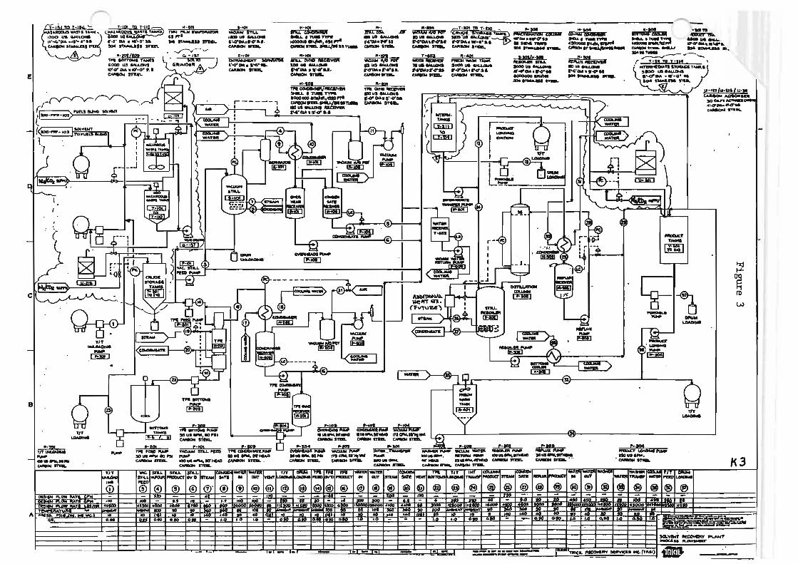
To properly select the computer model. the particular characteristics of e4ch accidental release scenario must be determined. The common process flow sheet. such as the one in Figure 3, should be reviewed to identify possible "release points", in much the same manner as fault tree analysis. Additional charscteristics to note are the physical dimensions of nearby structures and distances to property boundaries. as shown in Figure 4a. Also important is the type of release itself. As shown in Figure 4b, a liquid with a high vapor pressure leaking from a cylindrical tank into a diked area could result in an emission best characterized as a continuous release from a rectangular "ares" eource (as oppoaed to equa1'e or circular): or, depending on the liquid characteristics and peculiarities of the lea),. a "point" or "line" sour'ce type model ahould be used.
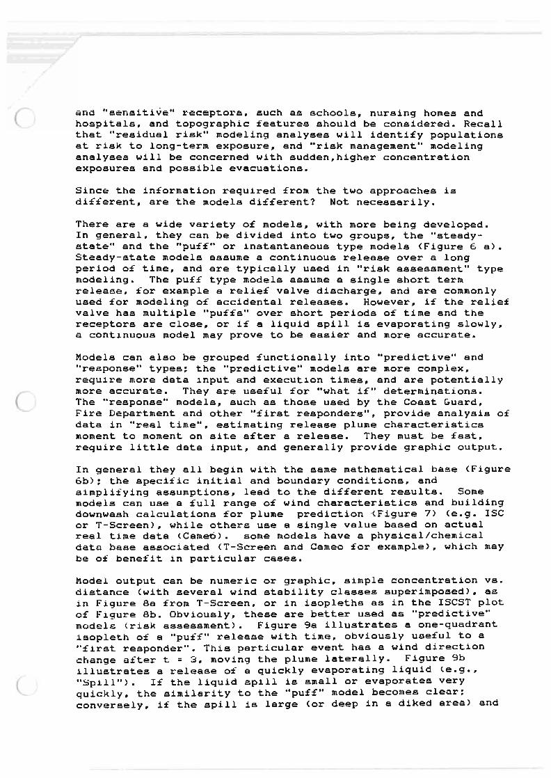
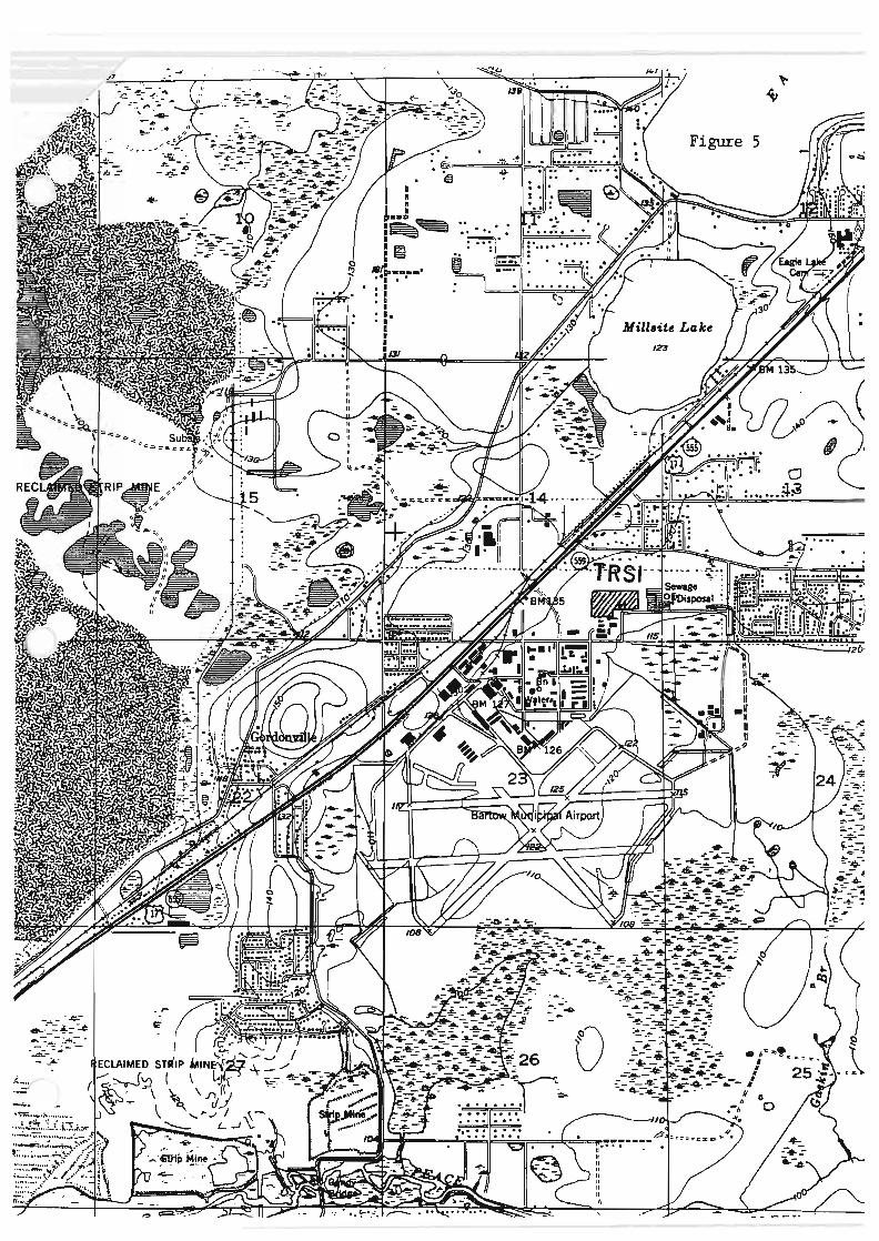
Also important is a review o£ the area surrounding the facility. as in Figure 5. Distances and directions to population centers
&ind "sensitive" r-eceptol'e. such as schools, nursing homes and hospitals~ and topographic features should be considered. Recall that "residual risk" modeling analyses will identify populations at risk to long-term exposure" and "risk management" modeling analyses will be concerned with sudden"higher concentration exposures and possible evacuations.
Since the information required from the two approaches is di£ferent, are the models different? Not necessarily.
There are a wide variety of models, with more being developed. In general~ they can be divided into two groups" the "steadystate" and the "puf£" or instantaneous type models (Figure IS a). Steady-state models assume a continuous release over a long period of time, and are typically used in "risk assessment" type modeling. The puff type models assume a single short term release. for example a relief valve discharge, and are commonly used for modeling of accidental releases. However" if the relief valve has multiple "puffs" over short periods of time and the receptors are close, or if a liquid spill is evaporating slowly, a contlnuous model may prove to be easier and more accurate.
Models can also be grouped functionally into "predictive" and "response" types; the "predictive" models are more complex, reqUire more data lnput and execution times" and are potentially more accurate. They are useful for "what i£" determinations. The "response" models" such as those used by the Coast Guard, Fire Department and other "first responders", provide analysis of data in "real time", estimating release plume characteristics moment to moment on site after a release. They must be fast, require little data input" and generally provide graphic output.
In general they all begin with the same mathematical base (Figure 6b); the specific initial and boundary conditions, and Simplifying assumptions" lead to the different results. Some models can use a full range of wind characteristics and building downwash calculations for plume prediction ~Figure 7) (e.g. ISC or T-Screen), while others use a single value based on actual real time data (CameO). some models have a physical/chemical data base associated (T-Screen and Cameo for example), which may be of benefit in particular cases.
Model output can be numeric or graphic, simple concentration vs. distance (with several wind stability classes superimposed), as in Figure 8a from T-Screen. or in isopleths as in the ISCST plot of Figure 8b. Obviously~ these are better used as "predictive" modele (risk assessment). Figure 9a illustrates a one-quadrant isopleth of a "puff" release with time, obviously useful to a "first responder". This particular event has a wind direction change after t = 3, moving the plume laterally. Figure 9b illustrates a release of a quickly evaporating liquid (e.g., ·'Spill") • If the liquid spill is small or evaporates very quickly, the similarity to the ··puff" model becomes clear: conversely, if the spill is large (or deep in a diked are~) and
(
evaporates siowly, a "continuous" type area model (ISCST - area or PAL) might be more attractive than a spill model.
The ultimate selection of the model depends on an understanding of:
1. the type of information required from the analysis - don't ask the model to do what it can't do (e.g., predictive or responsive?)
2. the 1nitial and boundary conditions and assumptions upon which the model algorithms are based-violate them with caution.
3. the real world phys1cal situation of the release - if it is a spill, does it evaporate quickly or slowly? Will it continue for a long time? What model types match the situation?
It is l~kely that several models will reasonably represent a particular situation. For example, Figure 10 might represent a "predictive" analysis of a trapezoidal area source, potentially modeled by the area source of ISCST or PAL, or by a circular pool of slowly evaporating liquid (Shell - SPILL or VAPOR). Figure 11 shows the calculated results. and it appears that for "nearby" receptors the "Spill" model. which is very easy to use. provl.des good agreement with the "higher accuracy" (and increased user effort) methods of ISCST.
Note that I said "appears". Actual data for both continuous and "puff" releases is very limited. and agreement of the various models is poor (unless one considers the monumental difficulties involved in obtaining an answer at all). Experimental results designed to test one model are frequently difficult to adopt to other models.
Despite careful selection of computer models, the results should be used with care, and several different models <preferably from different foundations) should be used to provide a "range" of probable values. The potential impact of these results on the :facility and operati6'ns should be evaluated long before the regulations are implemented. while sufficient time remains for proactive choices.
"RISK - BASED" "TECHNOLOGY -BASED
EMISSION STANDARDS
FOR HAZARDOUS AIR POLLUTANTS
NESHAPS MACT
FDER tlNTL" RESIDUAL RISK
ACCIDENTAL RELEASES (UNDER SARA)
ACCIDENTAL RELEASES
YEAR ONE-
YEAR TWO-
Figure la
LIST OF CATEGORIES AND SUBCATEGORIES OF MAJOR SOURCES - NOVEMBER 15, 1991
MACT STANDARDS AND LIST OF SPECIES FOR ACCIDENTAL ~ELEASE CONSIDERATION - NOVEMBER 15, 1992
YEAR THREE-
YEAR SIX-
PROMULGATION OF REGULATIONS PERTAINING TO AND REQUIRING RISK MANAGEMENT PLANS
-EPA REPORT TO CONGRESS ON RESIDUAL RISK FACTORS -FACILITY DEADLINE TO IMPLEMENT RISK MANAGEMENT
PLANS
YEAR ELEVEN-ESTABLISH REQUIREMENTS FOR RESIDUAL RISK-BASED
ADDITIONAL EMISSION REDUCTIONS
Figure Ib
( Initial List of Extremely Hazardous Substances . Under the Clean Air Act Amendments of 1990 . ammonia anh\'drous ammonia