RELIABILITY-OPTIMIZATION BASED MODELS F. Bouchart, N. Duan, I. Goulter K.E. Lansey, L.W. Mays, Y.C. Su and Y.K. Tung Book Chapter 1989 WWRC-89-22 In Reliability Analysis of Water Distribution Systems Chapter 14 F. Bouchart Department of Civil Engineering University of Manitoba Winnipeg, Manitoba, Canada I. Goulter Department of Civil Engineering University of Manitoba Winnipeg, Manitoba, Canada L.W. Mays Center for Research in Water Resources University of Texas Austin, Texas N. Duan Center for Research in Water Resources University of Texas Austin, Texas K.E. Lansey School of Civil Engineering Oklahoma State University Stillwater, Oklahoma Y.C. su Center for Research in Water Resources University of Texas at Austin Austin, Texas Y.K. Tung Wyoming Water Research Center University of Wyoming Laramie, Wyoming
Transcript
RELIABILITY-OPTIMIZATION BASED MODELS
F. Bouchart, N. Duan, I. Goulter K.E. Lansey, L.W. Mays, Y.C. Su and Y.K. Tung
Book Chapter 1989
WWRC-89-22
In
Reliability Analysis of Water Distribution Systems
Chapter 14
F. Bouchart Department of Civil Engineering University of Manitoba Winnipeg, Manitoba, Canada
I. Goulter Department of Civil Engineering University of Manitoba Winnipeg, Manitoba, Canada
L.W. Mays Center for Research in Water Resources University of Texas Austin, Texas
N. Duan Center for Research in Water Resources University of Texas Austin, Texas
K.E. Lansey School of Civil Engineering Oklahoma State University Stillwater, Oklahoma
Y.C. su Center for Research in Water Resources University of Texas at Austin Austin, Texas
Y.K. Tung Wyoming Water Research Center University of Wyoming Laramie, Wyoming
CHAPTER 14
RELIABILITY-OPTIMIZATION BASED MODELS
Francois Bouchart, Ning Duan, Ian Goulter, Kevin E. Lansey, Larry W. Mays, Yu-Chun Su and Y.K. Tung
14.1 RELIABILITY-BASED OPTIMIZATION MODEL FOR WATER DISTRIBUTION SYSTEMS
This section presents the basic framework for a model that can be used to determine the optimal (least cost) design of a water distribution system subject to continuity, conservation of energy, nodal head bounds, and reliability constraints. Reliability is defied as the probability of satis- fying nodal demands and pressure heads for various possible pipe failures (breaks) in the water distribution system. The overall model includes three models that are linked: a steady-state simulation model, a reliability model, and an optimization model. The simulation model is used to implicitly solve the continuity and energy constraints and is used in the reliability model to define minimum cut-sets. The reliability model which is based on a minimum cut-set method determines the values of system and nodal reliability. The optimization model is based on a generalized reduced gradient method. Examples are used to illustrate the model.
14.1.1 Previous Models
Numerous optimization models have been developed and reported in the literature. However, very few optimization models have included the reliability aspects in the design of water distribution systems. Damelin, Shamir and Arad (1972) developed a model to evaluate the reliability of supplying a known demand pattern in a given water supply system in
4 7 2
which shortfalls were caused by random failures of the pumping equip- ment. However, there is no optimization performed in their model and only p u p failures are considered. The major components considered in the Shamir and Howard (1979) model are the storage volume and the standby pumps.
Tung (1985) discussed six techniques for water distribution system reliability evaluation and concluded that the cut-set method is the most efficient technique in evaluating the system reliability of water distri- bution systems. Goulter and Coals (1986) developed a model in which they incorporated reliability aspects into a linear programming model. One disadvantage of the Goulter and Coals (1986) model is the assumption that all the pipes connecting a node have similar diameters and hence have similar values of the failure probability which is not applicable in real pipe networks. A second disadvantage is a theoretical weakness in the node isolation approach. The model considers a node to be adequately supplied as long as there is at least one link connecting it to the rest of the network. In addition, the model is not able to determine the design of pumps and storage tanks or consider multiple loading conditions.
Mays and Cullinane (1986) introduced methods for evaluating the reliability of individual water distribution system components which included the concepts of mean time to failure analysis and stress-strength or load-resistance analysis. They also concluded that the most promising methods for determining the system reliability and availability for simple series-parallel combination systems were the cut-set method and the path- enumeration method.
Wagner, Shamir and Marks (1986) developed a model for the calculation of probabilistic reliability measures for water distribution systems. They defined the term "reachability" to denote the situation when one specified demand node in the network is connected to at least one source. Since there are an exponential number of configurations which are used in searching and computing the reachability of demand nodes, methods for calculating these probability measures must be effi- cient which may not be applicable to large or even moderately sized, complex systems. Also, Wagner, Shamir and Marks (1986) could not include the multiple loading conditions into the model. Furthermore, this model did not incorporate the reachability aspects into an optimi- zation model for the design of water distribution systems.
14.1.2 Problem Description
The overall optimization problem for the design of water distri- bution networks considering the reliability aspect can be stated as follows:
4 7 3
Objective:
Minimize Cost f (D,L) (14.1.1)
subject to
Conservation of flow and conservation of energy constraints
(14. I .2)
Pressure head bound
(14.1.3) - H 2 H 2 H
Reliabilities constraints - for both system and demand nodes
R 2 R (14.1.4)
Non-negativity constraints
D20 (14.1.5)
where D is the pipe diameter; L is the pipe length; H is the nodal pressure head; and R is the reliability.
For a water distribution network design problem, the objective is to minimize the total cost of the network. The variables in the objective function are the nodal pressure head, H, the flowrate, Q, and the pipe dia- meter D. Also the pipe length, L, is a parameter in the objective function. Since the flowrate, Q, can be written in terms of H via the flow equation it does not appear in the objective function, equation (14.1.1).
The constraints of this optimization model are:
1. Conservation of Mass and Enerm - The total amount of water flow into a junction node should be equal to the total amount of water flow out from this junction node. For each junction node the continuity equation can be written as
CQh - Ca,, = Qe (j equations) (1 4.1.6)
4 74
where Qin is the flowrate of the water into the junction; Qout is the flow- rate of the water from the junction; Qe is the external demand at the junction node; and j is the number of junction nodes.
The conservation of energy constraint for each primary loop states that the sum of the energy loss in each pipe should equal to the energy put into the liquid. For each primary loop which is an independent closed path, the conservation of energy equation can be written for the pipe in the loop as follows
C h L = C E P (m equations) (14.1.7)
where hL is energy loss in each pipe, Ep is energy produced by a pump, and m is number of primary loops.
For f fixed grade nodes, f-1 independent conservation of energy equations can be written for paths of pipes between any two fixed grade nodes as follows
(f - 1 equations) (14. I .8)
where AE is difference in total grade between the two fixed grade nodes and f is the number of fixed grade nodes.
2. Head Bounds - The pressure head H at each demand node should be within a specified range of a minimum required head H and a maximum R:
- H 2 H 2 H for each demand node (14.1.9)
3. Reliabilitv Constraints - Both the system and nodal reliabilities should be greater than or equal to a lower bound which may be different for the different reliabilities.
Rs(H,D) 2 -s R for the network (14.1.10)
R(H,D) 2 R for each demand node (14.1 .I I)
4. Non-negativitv Constraints on pipe diameter, equation (14.1.5).
4 75
By using the formulation proposed by Lansey and Mays (1985) f ie above model can be used to determine the design of pumps and storage tanks while considering multiple loading conditions. The model here only considers the reliability aspect of the pipe network.
14.1.3 Model AIgori thm
Three models have been combined to develop the framework for a methodology to define the overall optimal (least cost) reliability based design of water distribution systems. A simple flowchart is presented in Fig. 14.1.1 illustrating the basic concepts of this methodology. The optimi- zation model used is the generalized reduced gradient model, GRG2, by Lasdon and Waren (1979, 1984) which solves an optimization problem with a nonlinear objective function and nonlinear constraints. A simu- lation model is used to implicitly solve the continuity and conservation of energy constraints, equation (14.1.21, at each iteration of the optimization procedure. The simulation model adopted is the University of Kentucky Model known as KYPIPE by Wood (1980) which simulates steady state flow in a water distribution system based upon the continuity and conservation of energy equations. The model determines the pressure head at each node satisfying continuity. A reliability model is used to determine the nodal and system reliabilities at each iteration of the optimization proce- dure using the minimum cut-set method. A minimum cut-set is a set of system components which, when failed, causes failure of the system but when any one component of the set has not failed, does not cause system failure (Billinton and Allan, 1983).
For each iteration of the optimization model (GRGZ), the reliability model computes the values of the system and nodal reliabilities based upon the minimum cut-set method. By assuming that a pipe break can be isolated from the rest of the system, minimum cut-sets are determined by closing a pipe or combination of pipes in the water distribution system and using the simulation model (KYPFE) to obtain the values of pressure head at each demand node of the system. By comparing these pressure heads with minimum pressure head requirements, the reliability model can determine whether or not this pipe or combination of pipes is a mini- mum cut-set of the system as well as of the demand nodes whose pressure head does not meet the minimum requirement. This procedure is repeated until all the combinations of pipes have been considered and hence all the minimum cut-sets of the demand nodes and the total system have been determined. The reliability model then computes the values of system and nodal reliability and returns to the optimization model.
The optimization model determines whether the solution is opti- mal or not. If not, the optimization model based on the reduced gradient
476
System Simulation Model .) System Reliability Model
(Minimum Cut Set Method) (Univ. of Kentucky Model) 4
Subroutine
GCOMP
F i g u r e 14.1.1 Flowchart of Reliability Based Optimization
Model of Water Distribution Systems
477
method determines a new solution point in the direction of improving the value of the objective function (minimizing cost) and a new iteration begins. The model stops either with an optimal solution or with a mes- sage that the solution is infeasible which means that at least one of the constraints cannot be satisfied.
14.1.4 The Reliabilitv Model
Water main failures, as pointed out by O'Day (1982), are principally due to excessive load, temperature or corrosion. Break rates are dependent upon pipe size, geographic location, method of pipe manufacture, soil type, etc. Kettler and Goulter (1983) have shown that the failure rate for cast iron pipes in Winnipeg, Canada, has a strong relationship with pipe diameter.
The method used herein to determine the probability of failure of individual pipes is similar to the procedure developed by Goulter and Coals (1986). The probability of failure of pipe j, Pj, can be determined using the Poisson probability distribution
P. = b e -Pi J
and
pj = rj Lj
(14.1.12)
(14. I. 13)
where pj is the expected number of failures per year for pipe j; rj is the expected number of failures per year per unit length of pipe j; and Lj is the length of pipe j.
Assuming there are n components (pipes) in the i-th minimum cut-set of a water distribution system then the failure probability of the j-th component in the i-th minimum cut-set is Pi,j which can be obtained by equation (14.1.12). The failure probability of the i-th minimum cut-set is
P(MCi) = n P i , j = P Pi,* ... p. j= 1 i, 1 c n (14.1.14)
The basic assumption is that the occurrence of the failure of the compo- nents within a minimum cut-set are statistically independent.
478
For example, if a water distribution network has four minimum cut-sets, MCI, MC2, MC3, and MC4 for the system reliability, the failure probability of the system, Ps, is then defined as (Billinton and Allan, 1983)
MC,UMC~UMC,UMC, S
= &Ci) i =1
- $ $ P( MC, n MC. i = l j= i+ l J
+ x P ( M C i n M C . n M C k i < j c k I
MC, n MC, n MC, n MC4 (14.1.15)
By applying the principle of inclusion and exclusion (Ross, 1985) which gives the upper bound of PSI equation (14.1.15) can be reduced to
MC, u MC, u MC, u MC,
= P ( MC1) + P ( MC,) + P ( MC3)
= P(MCi) i =1
+P(MC4)
Expressing equation (14.1.16) in a more general form as
P s = 2 P(MCi) i = l
then the minimum system reliability, Rs, is expressed as
M R S = I -Ps = l-&(MC.) 1
i =1
(14.1.16)
(14.1.17)
(14.1.18)
479
where M is the number of minimum cut-sets in the system. The same approach can be applied to compute the values for the nodal reliabilities.
The procedure of determining the reliability of a water distribution system based on the minimum cut-set method is as follows. For a given initial solution (pipe diameters), one of the pipes in the system is closed (a simulated break) which means that no flow can pass through this pipe. Then a simulation is performed using KYPIPE to determine the pipe flows and nodal pressures throughout the network. This simulation model implicitly satisfies nodal continuity so that the resulting pressure heads at demand nodes of the system are compared to see if they satisfy the mini- mum pressure head. If the pressure head at any one of the nodes in the system is below the minimum required level due to the closure (simula- ted failure) of this pipe, this closed pipe is a minimum cut-set of the sys- tem and the nodes whose pressure head does not meet the required level. This pipe is then opened and another pipe is closed and the simulation model is run again. This procedure is repeated until all pipes in the system have been considered.
The model then closes combinations of pipes simulating simul- taneous failures of two pipes and KYPIPE is run for each combination. If the resulting pressure head at any one of the demand nodes of the system goes below the required level, the closed pipes are a cut-set of the system and the demand nodes whose pressure are not satisfied. If any one of the pipes in this cut-set is already a minimum cut-set of the system, by defi- nition, this cut-set is not a minimum cut-set of the system; otherwise, it is a minimum cut-set of the system. A similar comparison is made for the demand nodes.
After all combinations of pipes have been considered by the above procedure, all the minimum cut-sets of both the system and the demand nodes are obtained. The values of the failure probability of each pipe is obtained by using the Poisson distribution as previously described. The probability of failure of a minimum cut-set is then equal to the product of the failure probabilities of the pipes of this minimum cut-set, assuming that the failures of pipes are independent. The system reliability is then obtained by equation (14.1.18). Similarly, the reliability of each demand node in the water distribution system can be obtained. Later in this sec- tion, examples are presented to illustrate that the simultaneous failure of combination of pipes may not have a major impact on the reliability of the system because of the small probability of the failures of combination of pipes.
The generalized reduced gradient code, GRG2, by Lasdon and Waren (1984) has been used to solve the optimization model. GRG2
480
requires a user-supplied subroutine GCOMP for the purposes of com- puting the constraint and objective function values of the decision variables, GCOMP can also be used to read in initial values of any user- required constants. GRG2 is a modular program written to provide dynamic memory allocation with all arrays set up as portions of one large main array so that redimensioning of arrays is never required.
Generalized reduced gradient methods such as GRG2 require an initial solution to start the optimization search. GRG2 does have the option of using an initial solution provided by the user or to start from an arbitrary solution, as determined by the lower bounds of the decision variables. If the initial solution is an infeasible solution, a phase I optimi- zation is initiated which minimizes an objective function consisting of the sum of infeasibilities until a feasible point is found. Once this is achieved, the actual objective function replaces the sum of infeasibilities and the actual optimization phase is initiated. Using an initial point provided by the user allows the inclusion of engineering judgment in selecting a good initial solution which may or may not be feasible. In either case, experi- ence has shown that a good user-provided initial point results in less computer time than initializing the algorithms from the lower bounds. Although the model is able to give an optimal solution to the problem, a global optimal solution can not be guaranteed. Multiple starting points could be used to obtain different local optimal solutions and the one with lowest cost would be chosen as the final design.
GRG2 like most nonlinear programming codes require the gradi- ents of the objective function and constraints with respect to the decision variables to determine search directions. Due to the way the reliabilities and the definition of a minimum cut-set must be determined, these gradi- ents cannot be computed analytically. A numerical scheme must be used which perturbs each decision variable individually, computes the objec- tive function and constraints for the perturbed values and then calculates the gradients, e.g., af/& = &/Ax.
14.1.5 Example Application
A hypothetical one-loop 14pipe network as shown in Fig. 14.1.2 is used to illustrate the model. This example has a requirement to design a least cost water supply network to satisfy the demands at thirteen demand nodes and meet the reliability constraints. The length of pipes and asso- ciated initial failure probabilities for an initial solution, with all pipe diameters being 36 inches, are listed in Table 14.1.1. The values of eleva- tion, demand and initial pressure of the nodes resulting from the initial flow and geometry condition are listed in Table 14.1.2. The pump in pipe 1
481
Figure 14.1.2 Water Distribution Network of Example
482
x w
00
00
00
00
00
00
00
o
oo
oo
oo
oo
oo
oI
no
0
~0
00
0~
0~
00
0m
P
rl
rl
dr
lr
l
rl
dr
lr
(
Table 14.1.2 Character is t ics of Demand Nodes
Node
Number
1
2
3
4
5
6
7
8
9
10
11
12
13
FGN
0.75
0.75
0.75
1.50
0.75
3.00
0.00
1.50
1.50
0.75
0.75
0.75
1.50
-14.25
Elevat i o n
( f e e t ) ~
2518.0
2517.0
2498.0
2492.0
2508.0
2523.0
2513.0
2532.0
2512.0
2520 .O
2540.0
2530.0
2552.0
2323.0
I n i t i a l Pressure
( p s i )
62.68
63.11
71.41
74.00
67.01
60.50
64.85
56.62
65.34
61.89
53.16
57.49
47.96
0.00
has a useful pumping power of 550 horsepower. The objective function for pipe cost (Quindry, Brill and Liebman, 1981) used in this example is
Minimize f (D,L) = 1.1 Df:24 L.. 'J '1 i,j
(14.1 22).
where Dij is the Pipe diameter (inches) and Lijis the pipe length (feet). The constraints are equations (14.1.6), (14.1.7), (14.1 -8) solved implicitly using KYPIPE and
Hi 2 92.3 feet (40 psi) (14.1.23)
Rs 2 0.80 for system (14.1.24)
R. 2 0.95 for all demand nodes (14.1.25)
for all demand nodes
1
D.. 2 0 'I
for all pipes (14.1.26)
The Hazen-Williams formula is used in KYPIPE to determine the pipe flows. A Hazen-Williams roughness coefficient of 130 is used for all pipes. English units are used for all computations. Note that the continuity and conservation of mass constraints are implicitly satisfied in the simulation model, and hence, the explicit constraints considered by GRG2 are equa- tions (14.1.23) to (14.1.26). A convergence tolerance of 0.001 is used for all constraints.
Using failure data obtained from the City of St. Louis (1985), a regression equation was developed to compute the average break rate, PR (breaks/mile/year), as
-0.1363D = 0.819e (14.1.27)
where D is the pipe diameter in inches.
The initial and optimal minimum cut-sets and values of reliability for the example system and for each demand node of the system are listed in Tables 14.1.3. The bptimal value of the objective function is $652,000. The final values of the pipe diameters and associated failure probabilities of the network are listed in Table 14.1.4. This example required 1,157 seconds for execution on the CDC Dual Cyber 170/750 mainframe system at The University of Texas at Austin.
485
Table 14.1.3 Minimum Cut-Sets and Reliabilities of the System and Demand Nodes
b
I n i t i a l Optimal
System System
R e l i a b i l it y Re1 i a b i l i t y
Minimum Cut S e t s of System
(Pipe Number)
1, 2 , 3 , 4 , 5 , 6, 8, 9, 11, 13,
7 & 10, 7 & 12, 7 & 14, 1 0 t 12, 0.88963 0.e39as
10 & 14, 12 & 1 4 .
486
P i p e
Number
Table 1 4 . 1 . 4 O p t i m a l S o l u t i o n for Example
Multiple P i p e Minimum Cut S e t s
Diameter
( i n c h e s )
F a i l u r e
P r o b i l i t y
1
2
3
4
5
6
7
8
9
1 0
11
1 2
1 3
1 4
3 6 . 0 0
22 .69
15 .95
17 .77
27 .07
21 .07
3 5 . 7 9
20 .29
29 .40
13 .98
11 .68
35 .13
20.39
9.77
0 .012530
0 .011481
0 .021315
0.019547
0 .014618
0 .017221
0 .008813
0 .017692
0 .009773
0 .023841
0.028074
0 .012681
0 .006206
0 .023500
S i n g l e P i p e Minimum C u t S e t s
Diameter
( i n c h e s )
36 .00
1 4 . 4 0
13 .15
12 .80
31.73
25 .30
21 .30
36 .00
36 .00
12 .93
11 .76
1 1 . 1 3
36 .00
12 .10
F a i l u r e
P r o b i l i t y
0.012530
0 .016322
0.025172
0.0257 93
0 .013360
0 .015239
0.011994
0 .012530
0 .008788
0 .025558
0.027894
0 .029391
0 .004404
0 .019091
487
The previous solution for the example computed minimum cut- sets considering the failure of single pipes and the simultaneous failure of two pipes. Considering simultaneous failure of two pipes has a small probability of occurrence and requires considerably more computational effort to compute the minimum cut-sets at each iteration of the optimiza- tion procedure. The example has been resolved considering only minimum cut-sets consisting of single pipe failures.
The nodal and system minimum cut-sets and reliabilities for the initial and final solution for the example are listed in Table 14.1.5. The optimal pipe sizes and associated failure probabilities for the examples are listed in Table 14.1.4. The optimal objective function values and compu- tation time for Example 1 are $651,690 and 1,157 seconds considering both single and simultaneous two pipe failures minimum cut-sets as opposed to the $622,470 and 515.1 seconds considering only single pipe minimum cu t-sets.
Pipes 7/ 10,12 and 14 are in a loop and are in minimum cut-sets for the simultaneous failure of two pipes but are not in minimum cut-sets when considering single pipe failures. The fact that these pipes are not in the minimum cut-sets for the single pipe failure case excludes them from the reliability constraints and causes the model to use larger size pipes in other locations such as pipes 5,7,9 and 13 in order to satisfy the reliability constraints.
The system reliability for the optimal design using both single pipe and siqultaneous failure of two pipes is 0.83985 as given in Table 14.1.3 and the system reliability using the single pipe failure is 0.83528 in Table 14.1.5. The last column in Table 14.1.5 lists the system and nodal reliabilities of the optimal design when considering both single and sim- ultaneous pipe failure. These values are not significantly different than those considering the single pipe failures. The difference in cost for these two design is $29,220 for a very small change in system reliability, 0.83985 as compared to 0.83797 for the design which considered single pipe mini- mum cut-sets. Comparing the nodal reliabilities in Tables 14.1.3 and 14.1.5, there are rather insignificant differences in the nodal reliabilities. The last column in Table 14.1.5 lists the system and nodal reliabilities using the optimal design (Table 14.1.4) based upon single pipe minimum cut-sets, but including the failure of both single pipes and two pipes failing simultaneously. This illustrates that when the minimum cut-sets of two pipes failing simultaneously are considered for this example that the system and nodal reliabilities are reduced only slightly. The small differ- ences in system reliability from considering only one pipe minimum cut- sets as compared to one pipe and then two pipes failing simultaneously;
488
Table 1 4 . 1 . 5 Minimum Cut-Sets and R e l i a b i l i t i e s of t h e System
a n d Demand Nodes ( S i n g l e Pipe Minimum C u t - S e t s )
Minimum Cut Sets of System
(Pipe Number)
1, 2, 3, 4, 5 , 6,
8, 9, 11, 1 3 .
i I n i t i a l O p t i m a l
Sys tem Sys tem
R e l i a b i l i t y R e l i a b i l i t y
System
R e l i a b i l i t y *
0 . 8 9 0 3 1 0.83797 0 . e3528
*Based upon t h e optimal d e s i g n (Table 1 4 . 1 . 4 ) for s i n g l e pipe
minimum c u t - s e t s b u t c o n s i d e r i n g t h e r e l i a b i l i t i e s for b o t h s i n g l e p i p e and two pipe f a i l u r e s .
Node
Number
1
2
3
4
5
6
8
9
1 0
11
1 2
1 3
489
I n i t i a l O p t i m a l Minimum Cut S e t s Nodal
Nodal Nodal (Pipe Number) R e l i a b i l i t y *
R e l i a b i l i t y R e l i a b i l i t y
0.9500 0.9500 1, 2, 5, 9. 0 .9574
0 .9662 0.9653 0.9638 1, 5, 9.
0 .9624 0 .9500 0 . 9 5 0 0 1, 4, 8 .
0 .9597 0.9597 1, 6, 8 . 0 .9624
1, 9, 1 3 . 0 .9743 0.9743 0.9725
0 .9500 0 .9500 1, 3, 9, 1 3 . 0 .9617
0.9787 0 . 9 7 7 1 I, 9 . 0 .9787
1, 8 . 0 .9749 0 .9749 0 .9749
1. 0.9875 0.9875 0 .9875
0.9787 1, 9. 0 .9787 0.9787
1, 9 . 0 .9787 0.9787 0.9774
1, 9, 11. 0 , 9 6 6 2 0.9508 0 .9508
however, this can result in rather significant differences in the cost of the optimal solution.
The suggested design procedure is to determine the optimal design of a network considering only single pipe failures. The reliabilities of optimal design are then computed with both the single and simultaneous pipe failures. If the decision maker finds these reliabilities unacceptable, the system can be redesigned considering both single and simultaneous failures. When making this decision two points should be kept in mind. First, the optimal solution consists of continuous pipe diameters and rounding to a discrete solution will slightly affect the cost and reliabilities of the system. Second, the pipe failure data is not perfect knowledge. When reviewing the reliability values, the number of significant figures which can be considered as accurate must reflect this knowledge.
14.1.6 Conclusion
An optimal (least cost) reliability based design and evaluation model of a water distribution network has been presented. The objective of the model is to minimize the cost of the water distribution system subject to continuity, conservation of energy, nodal pressures, and relia- bility constraints. The model has been used on a few simple networks to test its validity in designing water distribution systems. This model also can be used in optimizing the extension of an existing water distribution network by setting the diameter of existing pipes to constant values and optimizing the extension. The optimal design of the extension is a func- tion of the reliability of the existing system since the pipe breaks in the existing system may cause nodal head constraints not to be satisfied in the extension. The advantages of this model compared with other models in the literature are: 1) it has successfully included the reliability aspects into an optimization model; and 2) it can give an optimal (least cost) design of a water distribution system while simultaneously satisfying the continu- ity, conservation of energy, nodal pressure head bound, and reliability constraints. Additional details of this basic framework of the methodology presented herein can be found in Su (1986).
There are two disadvantages of the model. First, the resulting pipe diameters may not be commercially available pipe sizes so that these resulting pipe diameters must be rounded to the appropriate sizes. These rounding diameters might affect the feasibility of the resulting optimal solution and further research is being done to solve this problem. The second disadvantage is that the model can require considerable computa- tional effort to determine the optimal design of large looped networks. The computation time required for this model depends on the number of pipes and number of loops and to a lesser extent on the initial solution
490
used in the optimization. More research is in progress on reducing the computational time required to execute the model.
More research should also be done to incorporate other system components such as pumps, valves, storage tanks, etc. The major problem is how to define the reliability of a system which includes all these com- ponents. Also, a system under multiple loading conditions with normal demand conditions and emergency demands such as fire demands, should be considered in the least cost design model to ensure that the nodal pres- sures are met for these loads. Furthermore, research may be extend this model to incorporate the repair and replacement
performed to type analysis.
14.2 WATER DISTRIBUTION SYSTEM DESIGN UNDER UNCERTAINTIES
14.2.1 In trod uc ti on
A chance constrained optimization methodology is presented for the minimum cost design of water distribution networks. This method- ology attempts to account for the uncertainties in required demands, required pressure heads, and roughness coefficients. The optimization problem is formulated as a nonlinear programminggroblem which is solved using a generalized reduced gradient method. Details of the mathematical model formulation are presented along with example applications. Results illustrate that uncertainties in demands, pressure head requirements and roughness can have significant effects on the network design and cost.
There is currently no universally accepted definition or measure of the reliability of water distribution systems. In general, reliability is defined as the probability that a system performs its mission within specified limits for a given period of time in a specified environment. Over the past two decades, there have been many models developed for the analysis and the minimum cost design of water distribution networks (e.g., Alperovits and Shamir, 1977; Quindry et al., 1981; Morgan and Goulter, 1986; Lansey and Mays, 1987). Only a very few models have been reported that attempt to consider the reliability of the network and the various components. Coals and Goulter, (1985) presented three approaches by which the probability of failure of individual pipes can be related to a measure of the overall system reliability in a linear program- ming minimum cost design procedure. No models explicitly consider the uncertainties in demands, pressure heads, and pipe roughness.
49 1
The real issue of water distribution system reliability concerns the ability of the system to supply the demands at the nodes or demand points within the system at required minimum pressures. The conventional design process for water distribution systems is a trial and error procedure that attempts to find a design that represents a least-cost solution that can satisfy demands. These trial and error methods make no attempt to ana- lyze or define any reliability aspects of the designed system and have no guarantee that the resulting system is a minimum cost system. The resul- ting system design is not based upon consideration of the various design uncertainties.
Mays and Cullinane (1986) presented a review of methods that can be used to define the component reliabilities for the various components of a water distribution system. These methods are based upon using time- to-failure and time-to-repair data for the various components of the water distribution system to 'define reliability and availability. Su et al. (1987) presented a procedure for modeling reliability in water distribution net- work design that more realistically considers reliability. That is, the reliability is defined in terms of the ability of the system to supply the demands at the nodes or demand points within the system at or above minimum pressure heads. This model uses component failure rates to compute component failure probabilities which are then used to define nodal and system reliabilities. A minimum cut-set method is used in the nodal and system reliability detennination. The key issue in this approach was to relate failure probability of the pipes to meeting specified demands (flow rates) at minimum pressure heads at the demand nodes. The proce- dure was linked to a nonlinear programming optimization model to determine a minimum cost water distribution system considering nodal and system reliabilities as constraints.
Water distribution systems are designed to service consumers over a long period of time. Because the number and types of future consumers are impossible to define with any accuracy, the projected future required demands and required pressure heads for design are very uncertain. Ano- ther uncertain parameter in the design of a system is the system capacity. The capacity is affected by corrosion of pipes, deposition in pipes, even the physical layout and installation of the system which has a marked effect on the carrying capacity. The change in system capacity can be reflected in the roughness coefficient of the pipes (Hudson, 1966). Since the impact of the different mechanisms that decrease system capacity is not known, there is uncertainty in the projections of the coefficients of roughness. The variation of roughness is illustrated in the work by Hudson who compared the Hazen-Williams roughness coefficient for seven U.S. cities as a function of age of pipe.
492
No models have been developed for the minimum cost design of water distribution networks that directly consider the uncertainties in demand requirements, pressure head requirements, and roughness coeffi- cients. Previous models considered uncertainties in delivering flows and pressure heads during pipe failures. There have been many works reported in the literature that deal with uncertainties in water supply forecasting and modeling; however, very little work has been performed in developing a model that directly considers the uncertainties of required demand and other system parameters in the design of water distribution s ys tems.
The objective of this section is to present a methodology which incorporates the uncertainties in required demands, required pressure heads and roughness coefficients in the design of water distribution systems. In the technique, each of the parameters is considered as inde- pendent. The required demand, Q, and the required pressure head are dependent upon consumer needs whereas the roughness coefficient depends upon other factors, such as the types of pipes in the system, age, amount of deposition, etc. The methodology is presented through the formulation of an optimization model for the design of water distribution systems. This optimization model is based upon a nonlinear constrained fofiulation and can be solved d i n g generalized gradient methods, such as GRG2 by Lasdon and Waren (1984)# the mathematical model are given in addition to examples to methodology.
14.2.2 Model DeveloDment
Chance- reduced Details of
illustrate the
The basic optimization model for water distribution system design can be stated in general form as
Min. Cost = f(Di,j) i , jEM
subject to the following constraints
x h k = O
j = 1,. . ., J (nodes)
k = 1,. . .,K (loops)
(14.2.1)
(14.2.2)
(14.2.3)
(I 4.2.4)
i , j E k
H. 2 H. I 7
j = 1, ...,J
493
D.. 2 0 (14.2.5) 111
The objective function is to minimize cost as a function of the dia- meter Di,j/ for the set of possible links, M, connecting nodes i and j in the network. Constraint equation (14.2.2) is the continuity equation used to satisfy demand at each node in which q,j is the flow rate in the Pipe connecting nodes i and j, and Qj is the external demand at node j. This constraint is written for each node j in the network. Constraint equation (14.2.3) states that the sum of the head losses, hk, around each loop k = l,..., K is equal to zero. Equation (14.2.4) defines the lower bound, €3j , on the pressure head, Hp at each node.
The discharge q,j in each pipe connecting nodes i and j can be expressed using the Hazen-Williams, so that equation (14.2.2) can be expressed as
(1 4.2.6)
where K, is a constant to account for flow units; Ci,j is the Hazen- Williams roughness coefficient; Hi and Hj are the pressure heads at nodes i and j, respectively; Li,j is the length of the pipe connecting nodes i and j; and Di,jis the pipe diameter of the pipe connecting nodes i and j. Substi- tuting the Hazen-Williams equation into equation (14.2.2) makes equation (14.2.3) unnecessary since it is satisfied. The constraint set for the deter- ministic model now consists of equations (14.2.4, 14.2.5 and 14.2.6).
Considering the demands, Qk the minimum pressure head requirements, Ep and the pipe roughness coefficients, variables, the chance constrained formulation of the expressed as
Min.Cost = [f(Di,j)] i,jtsM
subject to
(14.2.7)
0.54 H. - H. (I 4.2.8)
j = 1, ...,J (14.2.9)
D.. 2 0 'PI
(I 4.2.1 0)
The objective function (14.2.7) is expressed in terms of minimizing the costs. Constraint equation (14.2.8) is expressed as the probability, P( 1, of satisfying demands, i.e. that demands are equalled or exceeded with probability level a.. Similarly, constraint equation (14.2.9) expresses the mobability of the minimum pressure head being satisfied, i.e. the pressure
1
heads bj-
14.2.3
equal or exceed the minimum pressure head with probability level
Deterministic Equivalent Form of Model
The above model (14.2.7) - (14.2.10) can be transformed to a deter- ministic form using the concept of the cumulative probability distribution. Although the theory is general and the variables may follow any distri- bution, the demands, Qk pressure minimum heads, H+ and roughness coefficients, Ci,p are assumed to be normal random variables, with means, p, and standard deviations, 0, expressed as
and
(14.2.11)
(14.2.12)
(1 4.2.13)
Constraint equation (14.2.9) can be written in terms of the standard normal random variable as
r 1
(14.2.14)
Using the definition of the cumulative probability distribution, this can be simplified to
495
(14.2.15)
in which F is the cumulative probability.
The deterministic form of constraint equation (14.2.9) can then be expressed as
Hi - %j 2 (Ja F (14.2.16)
Because PH., SH. and pj are all specified, this constraint can be written as a simple bound constraint
-J -J
(14.2.17)
Similarly, constraint equation (14.2.8) can also be expressed in a deterministic form. The first step is to rewrite the constraint in the following form
'(cqi,j-4 1 0) 2 aj (14.2.18)
H. - H.
[y and then express the pipe flow using equation (14.2.6)
(14.2.19) 0.54
Because both Qj and Ci!j are considered normal random variables and are assumed statistically independent, the term on the left side of the inequality
(14.2.20)
496
is also a normal random
and standard deviation
rr
variable with mean
(14.2.21)
Constraint equation (14.2.19) can now be written as
(1 4.2.23)
which can be simplified to
s L a . (14.2.24) J
The deterministic form of constraint equation (14.2.19) is then
(14.2.25)
in which pwj and owj are defined by equations (14.2.21) and (14.2.22),
respectively. If the standard deviations OQ, W- and oc are equal to zero, the parameters are known with certainty. -
The deterministic formulation of the chance constrained model is expressed by the objective function (14.2.7) and constraint equations (14.2.25), (14.2.17), and (14.2.10) as
497
Min. Cost = f ( Di,j) i,jEm
subject to
D.. 2 0 14
(14.2.7)
(14.2.25)
(14.2.17)
(I 4.2.1 0)
This is a nonlinear programming problem in which equations (14.2.17) and (14.2.10) are treated as simple bound constraints. Equation (14.2.17) is a simple bound because the right-hand side
is known as previously discussed. Constraint equation (14.2.25) expresses the relationship for the decision variables Hj and Di,j. The nonlinear problem consists of one nonlinear constraint (14.2.25) for each node and a simple bound for each decision variable, i.e., one for each pipe link and one for each node. The total number of decision variables is the sum of the number of nodes (number of €39 and the number of pipe links (number of diameters).
The model formulation assumes that the decision variables, H and D, are independent of the random variables, Qj, Hj, and C. This can be done through the zero order decision rule for chance-constrained pro- gramming (Charnes and Cooper, 1963; Charnes and Sterdy, 1966).
14.2.4 Solution Techniaue
The above deterministic model formulation of the chance con- strained model is nonlinear because of the nonlinear objective function and nonlinear constraints (14.2.25). The generalized reduced gradient code, GRG2, by Lasdon and Waren (1984) has been used to solve the deter- ministic form of the chance constrained model. This model is briefly described in section 14.1.
498
14.2.5 Example Applications
To illustrate the use of the model, two examples are included. The first is a simple hypotheticd network, shown in Fig. 14.2.1, which has two loops and eight pipes, each 3,280 feet in length, and mean demands at each node as shown in the figure. All the nodes are assumed to be at the same elevation and the pressure head at the source, node 1, is 196.8 feet. The mean nodal pressure head requirement at each node is 100 feet, and the mean Hazen-Williams roughness coefficient is 100 for each link. The formulation, however, does not assume that all nodes have the same pressure head requirement or that they are on a level plane. Also, a gen- eral network with one or more source nodes can be incorporated, if desired. The pipe cost equation used in both examples is
COST = 0.331LD’” (14.2.26)
where D is the pipe diameter in inches and L is the length of the link in feet. This equation is representative for thickness Class 23 cast iron pipe and includes the cost for purchasing, hauling, and laying (U.S. Army - Corps of Engineers, 1980). Any cost function, linear or nonlinear, could be used as equation (14.2.26) is used only for the purpose of illustrating the model application.
Several computer runs were made using various values of the standard deviation of the demand, pressure head, and roughness coeffi- cient, in order to illustrate the impact of different levels of uncertainty on the design cost. The standard deviation selected for the nodal demands were 0.0, 0.10, and 0.25 MGD. Selected standard deviations for the pressure heads were 0, 5, and 10 f t and for the Hazen-Williams roughness were 0,5, and 10. A standard deviation equal to zero refers to the case of no uncer- tainty, and the larger the standard deviation, the greater the uncertainty. Computer runs were made for various values of a and P ranging from 0.5 to 0.99. Using a = 0.5 (p = 0.5) is equivalent to using mean values of the nodal demands and the pressure heads. Higher levels of a and p refer to more stringent performance requirements so that the likelihood of system failure is reduced.
Figure 14.2.2 illustrates the impact of increasing the standard deviation of the roughness coefficient and the nodal demands, indepen- dently, while assuming the nodal pressure head requirement is known with certainty (OH = 0). With only Hazen-Williams roughness being uncertain (OH = 0 and OQ = o), as expected, the higher the reliability requirementTthe greater the cost of the design. The same is true for
-
499
1.0 MGD 1.0 MGD
2 1
7
8
3
* 1.0 MGD
5
6
Figure 14.2.1 Exampie I: Eight Pipe Network
500
420000 ~i i
410000
A
U P Y
4J UJ 0 u
400000
390000
380000
370000
360000
350000
340000
330000 0.5 0.6 0.7 0.8 0.9 1.0
Figure 1 4 . 2 . 2 C o s t vs R e l i a b i l i t y Requirement (%=o)
365000
355000
- 350000 1 a? Y
JJ (D 0 0
345000
340000
335000
330000 0.5 0.6 0.7 0.8 0.9 1.0
P Figure 14.2.3 Cost vs Pressure Head R e l i a b i l i t y Requirement
(0 =0 =o> Q C
501
different standard deviations of nodal demand and known Hazen- Williams roughness coefficient (OH = 0 and oc = 0). Figure 14.2.3 shows the change in cost with increasing-b for two standard deviations of nodal pressure and no uncertainty in the nodal demands or roughness coeffi- cients (OC = 0, OQ = 0 >. The same trend is apparent in this figure as seen in Fig. 14.2.2.
The optimal continuous diameters could be converted to discrete diameters by considering them as equivalent pipe diameters and deter- mining the lengths of two pipes which make up the link and have the same hydraulic characteristics. All of the optimal solutions were branched networks as expected for the optimal design of systems under a single demand pattern. The nonlinear programming problem for this example consisted of 16 decision variables, 6 nonlinear constraints, and 14 simple bounds. The computation time required to determine a design was approximately 2 seconds of CPU time on the University of Texas Dual Cyber 170/750.
The second application considered a more realistic size network consisting of 33 pipes and 16 nodes (Fig. 14.2.4) with the pipe lengths listed in Table 14.2.1. This system was also assumed to be on a level plane although this restriction is not necessary since the pressure head require- ment may be different for each node. The demand is assumed to be uniform throughout the system with a 1 mgd mean demand at each node. The pipe roughness has a mean of 130 for all pipes and the mean mini- mum pressure head requirement is 92.3 ft. at every node. The pressure head at the source node was fixed at 135.0 ft. The model was executed for values of a and p equal to 0.5,0.75, and 0.90, with the pipe diameters and total costs listed in Table 14.2.2. As in the previous example, the cost of the system increases with the reliability requirement. The networks for a$ = 0.5, 0.75 and 0.90 are presented in Figs. 14.2.5,14.2.6, and 14.2.7, respectively.
The nonlinear programming problem for this example consisted of 49 decision variables, 16 nonlinear constraints, and 49 simple bounds. The computation time required for a typical problem was 100 CPU seconds on the University of Texas Dual Cyber System. However, when computing the gradients in GRG2 the numerical finite difference scheme was employed. Analytically calculating the gradients of the constraints which can be written in a closed form would result in significant savings with the final computation time being about 20-25% of that required when using the numerical gradients.
Figure 1 4 . 2 . 5 Optimal Network f o r (a=P=0.50)
506
N
t
S O U R C E
(no t to scale)
Figure 14.2.6 I Optimal Network f o r (a=P=0.75)
507
N
t
S O U R C E
( n o t to scale)
Figure 14.2.7 Optimal N e t w o r k for ( a=p=o.gO )
508
Summary
In most of the previous sections of this report, the mechanical reliability of the system, i.e. the likelihood of component failure, and its effect on the hydraulic performance was the primary measure of a sys- tem's reliability. However, the hydraulic performance reliability is also affected by the uncertain nature of the demands placed on the system, as discussed in Chapter 8, and the uncertain rate of decay in the network, as reflected in the pipe roughness coefficients. Using a nonlinear chance constraint formulation, a methodology to consider these uncertainties has been developed. The approach is similar to the load-resistance analysis presented in Chapter 8 but considering the ability of the system to meet the user's demands on flow and pressure head rather than an individual element.
The application of the methodology showed that as the reliability measure increased, the cost of the system increased as did its ability to perform satisfactorily under a wider range of conditions. For a specific network, a relationship between cost and the reliability measure can be developed which will allow a decision-maker to better understand this trade-off. Thus, more informed decisions can be made which better reflect the goals of the decision-maker and the community.
14.3 RELIABILITY-CONSTRAINED PIPE NETWORK MODEL
14.3.1 Introduction
The explicit consideration of reliability is one of the most difficult tasks facing researchers working on the development of least-cost opti- mization design models for water distribution networks. Reliability has traditionally been addressed in a deterministic sense by providing redun- dancy in the form of loops within the distribution network. The existence of loops, however, provided a major difficulty for least-cost design models, which by their very nature would try to remove redundant or unnecessary loops in the search for minimum cost (Templeman, 1982). In many cases, the problem was overcome by specifying minimum allowable pipe sizes in all links (e.g., Alperovits and Shamir, 1977; Quindry et al., 1981). While connectivity is ensked by these minimum pipes, redundancy in terms of having adequate and independent flow paths to each node is not guar- anteed, and the resulting networks can operate as implicitly branched, non-redundant systems (Goulter et al., 1986). This redundancy problem has been partially overcome in the design models of Rowel1 and Barnes (1982) and Morgan and Goulter (1985) by consideration of a wide range of
509
loading conditions and pipe failure combinations such that every Iink was on a primary suppIy path for at least one design condition. The improve- ment in redundancy consideration was obtained, however, at the cost of mathematical exactitude within the technique.
There is, however, a critical factor missing in the way in which redundancy /reliability is considered in these models. Reliability of a water distribution network is also defined by the probability of the network fail- ing to perform, either through failure of one or more of its components, e.g., pipes or pumps, or through the demand on the system being greater than that assumed for design purposes. Very little research activity has been reported on the inclusion of these probabilistic issues in optimization design models for water distribution networks. This section reports on a means of incorporating these probabilistic issues in iterative procedures based upon network design models.
14.3.2 Problem Statement
Most of the approaches to the probabilistic aspects of reliability in water distribution systems can be separated into two main groups. Inclu- ded in the first group are those approaches and models which address the reliability of the system as a whole. These approaches examine the relia- bility of the major components, namely, the supply, treatment, and distribution stages, in terms of the performance of the overall system. These problems are addressed by Hobbs (19851, Shamir and Howard (1985), Germanopoulis et al. (1986), and Hobbs and Beim (1986).
The approaches and models in the second group are directed at the reliability of specific components of the overall system, e.g., the distribu- tion network. This section discusses issues related to the reliability of the distribution network only and as such falls into this second area. The concepts examined relate to pipe size choice and its role in determining the network reliability. Some of the earlier work in the field of distribu- tion network reliability examined the reliability question in terms of the probability distribution of the demand on the network and the implica- tions of the flow required within a pipe exceeding its design capacity, e.g., Cullinane (1986) and Tung (1986). Wagner et al. (1986) examined the reliability of the network by looking at the actual shape or layout of the network. Studies by Goulter and Coals (1986), Cullinane (19861, and Mays et al. (1986) addressed the reliability question through use of the probability of individual pipe failure. Both Goulter and Coals (1986) and Mays et al. (1986) also showed how the concept of pipe breakage probability could be incorporated into a least-cost model for water distribution network design.
510
In this paper, the least-cost design models of Alperovits and Shamir (1977) and Goulter and Coals (1986) are combined and extended to recog- nize the probabilistic nature of the reliability issue. The extension is achieved through the introduction of reliability constraints, and by the inclusion of probabilistic factors in the coefficients in the formulation. The reliability constraints restrict the probability that the number of pipe breaks in a particular link in a given time period is greater than an accep- table value. Restrictions on the probability that the required flow in a pipe is greater than its design capacity is achieved by modifications to the flow values used in the formulation.
A network design provided by an optimization model incorpora- ting these reliability constraints is, however, only the least-cost "solution" for the probabilistic parameters applied through reliability constraints and the model coefficients. Furthermore, the probabilistic values do not in themselves give true or exact measures of the red network reliability. A series of computational steps are required to convert the probability values into reasonable measures of overall system performance. Various numerical expressions which can be used to guide changes to the model parameters such that the solutions obtained achieve improved overall reliabilities at least cost, are examined and evaluated in the following sections.
14.3.3 Model Formulation
The procedure is primarily based upon the least-cost linear program design model of Alperovits and Shamir (1977), which can be summarized as follows:
Objective Function:
subject to
Length Constraint:
N g i ) A L.. = LNi
'I j= 1 for all links i
(I 4.3.1)
(14.3.2)
511
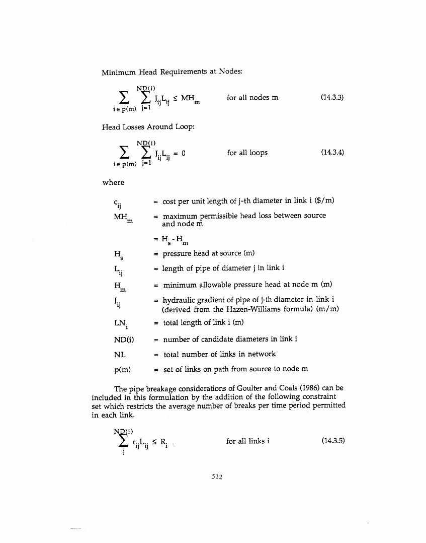
Minimum Head Requirements at Nodes:
for all nodes m m
Head Losses Around Loop:
c Ng;ijLij = 0 i E p(m)
where
C.. '1
MH m
H
L.. 'I
H m
S
Ji j
LNi
ND(i)
NL
p(m>
for all loops
(14.3.3)
(14.3.4)
cost per unit length of j-th diameter in link i ($/m)
maximum permissible head loss between source and node m
HS - Hm pressure head at source (m)
length of pipe of diameter j in link i
minimum allowable pressure head at node m (m)
hydraulic gradient of pipe of j-th diameter in link i (derived from the Hazen-Williams formula) (m/m)
total length of link i (m)
number of candidate diameters in link i
total number of links in network
= set of links on path from source to node m
The pipe breakage considerations of Goulter and Coals (1986) can be included in this formulation by the addition of the following constraint set which restricts the average number of breaks per time period permitted in each link.
ND i )
r..L.. 2 Ri . ' 'I 1J i for all links i (14.3.5)
512
where
r.. = 'I
Ri =
average number of breaks per year per unit length for j-th diameter pipe in link i (breaks/year/m>
maximum acceptable average number of pipe breaks per year in link i
Probabilitv Distribution of Pipe Breakages
The formulation described by equations (14.3.1) - (14.3.5) does not have any recognition of the probabilistic features of either the rij factors or the Q k demand characteristics. In order to incorporate these probabilistic issues, the formulation must be modified as follows. The rij in equation (14.3.5) is the number of failures per unit length for a particular pipe dia- meter, which may vary significantly from year to year. In order to restrict the probability that the number of breaks in a link in any given year is greater than some acceptable value, equation (143.5) can be rewritten as follows
Nf)rijLij I mi j= 1
for all links i
where
- RHS, -
VAR(rij) =
(14.3.6)
inverse of the cumulative distribution function of r..
1J
probability of the number of breaks per year in link i
variance of r.. 'I
Probabilitv Distribution of Demand at a Node
In designing a water distribution network, the flow demands that must be provided at minimum specified pressures are generally taken as deterministic values. Little or no consideration is given to the possibility of these demands being exceeded. A more realistic view of the design flows, however, would recognize that the demands themselves are
513
probabilistic and that there is a finite probability that the demands on the system will at some time be greater than the design capacity. For example, one criteria for design flows may be the 10-year, 1-day maximum demand. The 20-year, I-day maximum demand will be larger than this value and is likely to occur at least once during the life of the distribution system.
Once the actual demand exceeds the design capacity, at least ont in the network will be required to carry a flow greater than its design capacity. Two situations can arise from this condition. The pipes can deliver the flow but at pressures below the minimum specified or the
? link
pipes will not be able t; provide the flow at all. Either kituation represents a "failure" of the network.
Tung (1986) approached the problem by assuming that the required demand and head at a demand node are random variables, with known probability distributions. A series of chance constraints for the demands and pressure heads at each node could than be formulated for inclusion in a least-cost design model. The approach used in this model does not allow the use of explicit chance constraints for these flow issues. Rather, the probabilistic component is addressed through inclusion in the coefficients of the model that are directly related to flow, e.g., Jij.
The actual incorporation of flow is achieved through the use of the following equation to define the demands at each node.
value of the demand at node k to be used as the design flow (volume/unit time)
avera e (ex cted) value of demand at node % (vocme/unit time)
standard deviation of demand at node k (volume/unit time)
inverse of the cumulative distribution function of Q,
probability that demand at node k will exceed the design demand
Solution of the optimization formulation described by equations (14.3.11, (14.3.3), (14.3.4), (14.3.6), and using the hydraulic gradient Jij values
5 14
derived from (14.3.7) provides a least-cost network with explicit consider- ation of both breakage or mechanical based reliability issues and flow exceedance probabilistic reliability measures contribute to the assessment of reliability. However, as mentioned earlier, the probabilistic measures contained with equations (14.3.6) and (14.3.7) are, however, only surrogates for the true reliability of the system, and do not give a real indication of the reliability of the network. The means to combine the two measures into a single comprehensive measure of pipe network reliability is yet to be available. Once a network solution has been obtained from the optimization model, it must therefore be examined to see if it contains satisfactory levels of reliability as assessed by the design engineer. If the network is judged to have satisfactory reliability, the problem is solved. If, on the other hand, it is felt that the network is unsatisfactory, then adjust- ments must be made to the parameters of the least-cost optimization model and the network solved again.
The question now arises as how to change the parameters of the model such that the requested improvements in reliability are obtained at the smallest increase in cost. In other words, a method which provides a measure of the sensitivity of the least-cost solution to changes in "relia- bility" oriented model parameters is needed. Before proceeding with an examination of these methods, it is important to note that there are a number of similarities in the way in which improvement to one of the measures of reliability causes improvements to other measures.
A number of researchers, e.g., Clark et al. (1982), Ciottoni (1983), and Kettler and Goulter (1985) have shown that pipe failure rates are strongly related to diameter with the larger diameter pipes having lower rates of failure than pipes with smaller diameters. Improvements to the pipe breakage or mechanical reliability can therefore be achieved by selecting larger diameter pipes. However, these larger diameter pipes also have greater hydraulic capacities for the same pressure conditions and therefore also provide increased flow capabilities. These increases in the flow capa- bilities reduce the probability that the flow required in a link (derived from demands at nearby nodes) will be larger than its design capacity. Similarly, improvements (reductions) to the flow exceedance probabilities at nodes will also improve mechanical reliability by causing the selection of larger diameter, high capacity, pipes which, in turn, have reduced rates of breakage.
Under such conditions, it might be expected that unsatisfactory sys tem reliability can be identified and improvements subsequently achieved through modifying either the mechanically based Ri and F-l(y) parameters in equation (14.3.6) or the flow exceedance reliability based F- 1(pk) parameter in equation (14.3.7). Unfortunately, this is not generally
5 15
true. Areas with good mechanical reliability may in fact have low flow- based reliability probability. Consider a pipe near a source. The pipe % likely to be of large diameter as it carries flow for a large downstrem portion of the network and will therefore have a low failure rate and correspondingly high mechanical reliability. The same pipe, however, may have a low flow exceedance-based reliability if the probability of 5 e flow exceeding the design capacity is relatively large.
It can be seen, therefore, that while there is some complementarv interaction between the two reliability conditions, care must be taken to ensure that areas of low reliability are always identified and the correct steps to overall system improvement undertaken. The following sections examine a number of ways of identifying system parameters which should be changed in order to achieve improvements to system reliability at least increase to sys tem cost.
14.3.4 Means of Improving System Reliabilitv - -
There are two major issues which must be examined in determin- ing how to improve system reliability. The first is which measure is to be used to define system reliability. The second is which parameters should be modified in order to achieve the desired improvement in reliability. Unfortunately, relatively little is known about either problem. Most optimization design models simply provide a network solution that may or may not address the probabilistic reliability issues of this paper. Gen- erally, no assessment of reliability is provided, and furthermore, no attempt is made to modify model parameters if reliability should be unsatisfactory.
Cullinane (1986) suggests a measure for system performance which considers both the mechanical reliability of the network components and the implications of failures of those components on the hydraulic perfor- mance of the network relative to its design criteria. The measure was not incorporated into an optimization design model. No indication was given on how to identify or change model parameters such that the desired improvements to network reliability were achieved with the lowest cost implications. Goulter and Coals (1986) developed optimization based procedures which use a mechanical reliability measure to define system reliability in t e r n of the probability of node isolation, i.e., the probability of all links connected to a node failing simultaneously. A means of deter- mining which link in the vicinity of the node has the worst probability of node isolation to change in order to obtain improved system reliability (reduced probability of node isolation) at least-cost was also provided. The measure used to identify the link for which the optimization model para- meters were to be changed was derived from the dual variables in the
516
linear programming solutions and the expected number of breaks in the links connected to the critical node.
It is important to note, however, that while the work of Goulter and Coals (1986) was one of the few to address the criteria for improving distri- bution network reliability, it was very simplistic and took no account of either the flow exceedance issues in network reliability or the probability distribution of the rates of pipe breakage. One of the primary features examined in this section is how to combine the mechanical and flow based reliability factors to provide a balanced measure for identifying how to modify the parameters in equations (14.3.6), and (14.3.7). There are, how- ever, similarities between the method of Goulter and Coals (1986) and the problems of the two reliability measures which can be exploited. Goulter and Coals (1986) lower the deterministic Ri values in their model in order to achieve the desired improvements. A reduction in y in equation (14.3.7) has the same general effect, although it achieves it through a probabilistic measure. The dual variable based method of Goulter and Coals (1986) therefore appears to have some applications to this extended problem and is used as the basis for three of the following measures.
At present, there is no explicit means of combining the two proba- bilistic failure measures in either a general statement of system reliability or in a single explicit measure which can be used to guide changes to the optimization to achieve more reliable networks. For this reason, a series of overall system reliability and improvement measures are formulated and critically compared.
The reliability measure chosen to assess system performance is a heuristic measure termed "the probability of 'node failure'.'' This mea- sure incorporates both pipe and demand failure through the following express ion
P(no "node failure") = P(no "node isolation") . P (no "demand failure") (14.3.8)
where P( ) = probability of Occurrence of event.
It should be noted that the term P(no "node isolation") is the relia- bility measure developed by Goulter and Coals (1986). However, in this case, the simplistic consideration of node isoIation is improved by com- bining it with the flow based probability measure P(no "demand failure").
The next problem is that if any part of the network is considered to be unreliable, according to equation (14.3.8), how should the parameters of the optimization model be modified in order to achieve the desired
5 1 7
improvement? One obvious consideration is that any improvement in reliability should increase the overall network cost. However, before proceeding with examination of the methods used to identify the appro- priate model changes, it is necessary to define a new parameter. Let WBi represent the "relative importance" or weighting of link i in the network. In the context of this paper, the relative importance of a particular link is determined by how much flow that link carries relative to the flows in other links of the network. The actual value of the weight for a particular link is calculated by
Flow in link i Total demand in network
WB, = (14.3.9)
The range of measures which were examined as to their suitability for determining how to improve the network reliability is described in Table 14.3.1. It should be noted that application of each measure requires that the portion of the network which has unsatisfactory reliability be identified. Within the table, the measures are described in relation to the reliability at the single node, k, having the worst "reliability" (as defined by equation 14.3.8) and those links connected directly to that node are to be addressed by the measures. The measures are, however, generally appli- cable to more than one node at a time, with the appropriate connections being examined in each case. The description relative to a single node is for simplicity in explanation only.
14.3.5 Application of Methodolodes
The measures were assessed by application to the network shown in Fig. 14.3.1. The pertinent data for the network is given in Tables 14.3.2- 14.3.4. All links in the network have total length of 1,000 m.
As equation (14.3.6) is nonlinear, the model cannot be solved directly by linear programming. It can obviously be solved by nonlinear optimization approaches. However, since the value of the dual variable is a crucial element in most of the improvement measures examined (see Table 14.3.1)' and the nonlinearity in equation (14.3.6) is not "severe," linear programming with successive approximations was used. Experi- ence with the formulations and this solution approach showed the combination to be very efficient.
In applying the model to the sample problem, the following "step sizes" were used to modify the model parameters when reliability was deemed to be unsatisfactory. For modifications (reductions to a particular value Ri, a step size corresponding to 10% of the initid Ri was used. For
5 18
Table 14.3.1 Description of Measures to Determine How to Improve Network Reliability
Means of Determining Means of Affecting Measure Which Link to Change Improvement
A Link with aCOST/aRHS Decrease the value of Ri for value, i.e., link minimum dual variable for equation (14.3.6)
link selected
B
C
Link with minimum value of link selected
Decrease the value of Ri for
BR, WB,
where BRi = actual number of breaks per unit time in links (= RHSi when equation (14.3.6) is binding for that link)
Link with minimum value of link selected
Decrease the value of Ri for
aCOST/aRHS. 1
where a(Relk) / aRHSi = rate of change in probability of isolation of node k with change is RHSi for link i (Goulter and Coals, 1986, measure)
D N.A. Increase confidence interval of demand at node by decreasing the value of bk
519
SOURCE
LEGEND:
A Link Number
-0- Node Number - Direction of f low in Link
Figure 14.3.1 Layout of Example Problem
Table 14.3.2 Demand Characteristics of Each Node
Elevation of Minimum Average1 Standard Deviation
(m> (m) (m3/hr) (m3/hr) Node Node Pressure Head Demand of Demand
12 100.0 0.077 IThese flows correspond to a demand confi- dence of 80% for all nodes, i.e., Pk = 0.20 for all k = 1,2, ..., 9
521
Table 14.3.4 Pipe Cost and Breakage Data
Diame terl Cost Average Number of Variance of Breaks (mm) ($/m) Breaks per yr per km per yr per km
25 (1.0)
51 (2.0)
76 (3.0)
102 (4.0)
152 (6.0)
203 (8.0)
254 (10.0)
305 (12.0)
356 (14.0)
406 (16.0)
2.0
5.0
8.0
11.0
16.0
23.0
32.0
50.0
60.0
90.0
1.552
1 .so
1.45
1.35
1.05
0.75
0.40
0.10
0.082
0.062
0.0262
0.023
0.023
0.020
0.012
0.006
0.014
0.01 4
0.0142
0.0172
457 (18.0) 130.0 0.052 0.0172
508 (20.0) 170.0 0.042 0.0202
559 (22.0) 300.0 0.042 0.0232
610 (24.0) 550.0 0.042 0.0262
IDiameters are given in millimeter equivalents of pipes whose diameters are given in inches in the parentheses alongside each value.
2These values are estimates, other values are taken from the work of Kettler and Goulter (1985).
522
modifications to confidence level of demand Pk at a particular node k, the following successively tighter confidence levels were used: 80% (initial value), 90%, 95%, 97.5%, 99%, 99.5%, and 99.9%. Whenever it was neces- sary to change the demand at a particular node to improve network reliability, for example, by using measure D, the resulting design flow in each link was calculated using the formulae listed in Table 14.3.5.
A summary of the results obtained from each measure is given in Table 14.3.6. The lengths and diameters of the pipes selected using each measure are described in Tabie 14.3.7. The base solutions in Tables 14.3.6 and 14.3.7 correspond to the solution with Pk = 0.20 and no pipe breakage constraints (equation 14.3.6) binding. The termination criterion for each measure, i.e., the point where the network was considered to have satis- factory reliability, was maximum probability of no node failure 2 65%. It was not possible to get the probabilities of no node failure to be exactly 65%. With the exception of measure XI@), the values shown in Table 14.3.6 represent the closest that the probabilities could be matched without using unrealistically high numbers of runs with minor modifications to the appropriate parameters.
The different results shown for D(a) and D(b) in Table 14.3.6 arise from use of a different stopping criterion. The criterion for D(a) was the same as for Measures A, B, and C, namely the probability of no node failure 2 65%. The D(b) case arose from examination of the results for D(c), ,which, relative to the results for the other measures, showed a higher number of expected breaks per year. With Db), an attempt was made to see if a solution with a greater cost than that obtained for Measures A, B, and C would result in a smaller number of expected breaks per year. It can be seen that such a result was not obtainable under the speafied conditions.
Discussion of Results
Examination of the results show that there is very little difference between the solutions obtained by measures directed at improving the reliability by modification to links, Lea, for Measures A, B, and C. The dif- ferences between the results is within the accuracy of the solution given the estimates of the parameters used in the formulation. The overall similarity of the results for the three measures suggests that if "link improvement" methods are to be used, the simplest measure, namely Measure A, is most appropriate.
Both applications of Measure D, which is the only measure directed at flow rather than component failure, produced improvement to the reliability at less cost than either of Measures A, B, or C (see Col. 3 of Table 14.56). This observation suggests that Measure D is the most efficient
523
Table 14.3.5 Formulae to Determine Design Flows in Each Link
Link Flow In Link
Table 14.3.6 Summary of Results
Cost Worst P (no AP(no "node ExpectedNo. Solution ($ x 103) "node failure") failure") of Breaks per
(%I A Cost Year in Network
Base solution 337.5 55.7 - 7.621 (80% flow confidence level and pipe breakage constraints not binding)
Measure A 359.1 65.4 2.72 '6.755 Measure B 359.7 65.5 2.62 6.744 Measure C 360.4 65.8 2.66 6.775 Measure D(a) 354.4 67.7 4.30 7.111 Measure D(b) 363.9 70.0 3.29 6.901
5 2 4
1
Table 14.3.7 Lengths and Diameters of Pipes Selected
1 Base Solution
254 563 305 437 203 1000
356 1000 152 491 203 231 254 278 152 107 203 893
152 320 203 548 254 132
A
254 305 152 203 254 356 152 203 254 203 254
152 203 254
~-
563 437 71
461 468
1000 491 231 278 323 677
320 548 132
B Diam.1 Length (mm) (m>
254 305 152 254
356 152 203 254 152 203 254 152 203 254
563 437 66
934
1000 431 343 226 265 376 359 304 579 117
Measure C
254 305 254 305
356 152 203 254 152 203 254 152 203 254
563 437 862 138
1000 308 571 121 479 203 319 270 642 88
254 320 305 680 203 427 254 573
356 1000 152 185 203 799 254 16 203 1000
152 152 203 848
Diam.1 Length (mm) (m)
305 1000
203 41 5 305 585
1000 356 152 167 203 833
203 1000
152 52 203 948
Table 14.3.7 (cont'd)
Measure Link
7
8
9 LJl rJ m
10
11
12
Base Solution Diam.1 Length (mm) (m)
152 203 254 254
152 203 254 152 203
203 254 152 203 254
612 7
381 1000
433 339 228 167 833
400 600 346 501 153
A
152 203
254
152 203 254 152 203 254 203 254 203 254
167 833
1000
433 339 228 42
836 122 400 600 72
928
13 Diam.1 Length (mm) (m)
152 203
254
152 203 254 152 254
203 254 203 254
167 833
1000
493 228 279 282 718
400 600
357 643
152 203
254
152 254
152 203 254 203 254 203 254
167 833
1000
615 285
225 497 278 400 600 72
928
152 203 254 254 305 152 203 254 203
203 254 152 203
253 673 74
763 237 185 799 16
1000
282 71 8 40
960
Diam.1 Length (mm) (m)
152 140 203 860
305 663 356 337 152 242 203 694 305 64 203 1000
203 200 254 800 203 1000
IThe actual pipe diameters used were in Imperial units (in), reflecting the availability of break records for these pipes. The values given in this table are the "rounded-off' metric equivalents of those diameters.
measure to use to improve node reliability. Its use appears to provide more flexibility in the choice of pipe diameters. Part of this flexibility is due to the fact that the improvement is not directed at a single link connected to the node of interest,'but rather to a region of the network where the reliability problem exists. As described in Table 14.3.5, increases in the design demand affect flows and subsequent pipe choices throughout the network. This "broad-scale" approach seems to permit the optimiza- tion model to adjust large sectors of the network resulting in cheaper networks for the same cost. This "broad-scale" approach is also intuitively more attractive, as it recognizes relationships within the network as a whole.
It is also interesting to note that both applications of Measure D do not reduce the expected number of breaks per year to the same extent as the first three measures. If reduction in number of breaks per year is an underlying objective of the problem, this feature may be considered a weakness. The smaller reduction in breaks required to achieve the better reliability does, however, support the general conclusions in the previous paragraph. Improvement in network reliability has not been achieved simpiy by the "mechanical" improvement used by the other three methods. The improvement in reliability is achieved by a more compre- hensive consideration of network performance.
Based on the above features of the four measures, it appears that Measure D is the best approach to use to improve network reliability. These conclusions are tentative, however, as they may be a function of the network chosen and the heuristic reliability measure chosen. The relia- bility measure of probability of "no node isolation" is, however, one of the most comprehensive measures for pipe network reliability currently available in that it explicitly recognizes both the pipe breakage and demand exceedance issues of the reliability question.
14.3.6 Summarv
A general philosophical framework for approaching the reliability issue is the design of optimization-based network design models. The framework uses a general optimization model which includes considera- tion of the probability of component, in a particular pipe, failure and the probability that the actual demand at a node will exceed the design value. The component failure issue is addressed through a set of chance con- straints which defines acceptable levels for probability of pipe breakage. The probability of demand at node being greater than the network capacity to supply is addressed through the use of probabilistic-based flow values from which the model parameters, such as hydraulic gradient, are derived. A new "measure" describing the reliability of the networks in terms of the
52 7
probability of "no node failure" has been developed and included in the overall approach. Although the measure is heuristic, it explicitly com- bines mechanical, e.g., pipe, failure probabilities and the probability of a "failure" caused by demand being greater than the design value.
A series of measures which can be employed to guide modification to network design to achieve improvements in reliability at least-cost were investigated. Based upon the results of application to a sample network, it appears that improving the probability that design capacity is greater than or equal to actual demand, as opposed to reducing the probability of com- ponent failure, provides the most improvement in reliability at least cost. If, however, reduction in the expected number of pipe breaks within a network over a given time period is a critical issue, measures which address the probability of pipe failure appear to be more appropriate.
These conclusions are preliminary, however, and further work on a wider range of networks is needed before any general recommendations can be made.
REFERENCES
Alperovits, E. and U. Shamir, "Design of optimal water distribution systems," Water Resources Research, Vol. 13, No. 6, pp. 885-890, 1977.
Billinton, R and R.N. Allan, Reliabilitv Evaluation of Enqineering Systems: Concepts and Techniaues, Pitman, London, 1983.
Charnes, A. and W. Cooper, Deterministic Equivalents for Optimizing and Satisfying Under Chance Constraints, Operations Research, Vol. 11, No. I, pp. 18-39,1963.
Chames, A. and A. C. Sterdy, "A Chance-Constrained Model for Real- Time Control in Research and Development Management," Management Science, Vol, 12, No. 8, pp. B-353 to B-342, April 1966.
Ciottoni, A.S., "Computerized data management in determining causes of water main breaks: The Philadelphia case study," Proceedings of the 1983 International Symposium on Urban Hydrology, Hydraulics, and Sediment Control, University of Kentucky, Lexington, Kentucky, pp. 323-329, 1983.
City of St. Louis, "1985 Main Break Report,'' Water Division, City of St. Louis, Missouri.
528
Clark, R.M., C.L. Stafford and J.A. Goodrich, "Water distribution systems- A spatial and cost evaluation," journal of the Water Resources Planning and Management Division, ASCE, Vol. 100, No. WR3, pp. 243-256, 1982.
Coals, A. and I.C. Goulter, Approaches to the Consideration of Reliability in Water Distribution Networks, Proceedings, 1985 International Symposium on Urban Hydrology, Hydraulic Infrastructures and Water Quality Control, University of Kentucky, Lexington, Kentucky, pp. 287-295, July 23-25,1985.
Cullinane, M. J., "Hydraulic reliability of urban water distribution systems," Proceedings of ASCE Conference, Water Forum '86: World Water Issues in Evolution; Volume 2, Edited by M. Karamouz, G. Baumli, and W. Brick, AXE, New York, New York, pp. 1264-1271,1986.
Damelin, E., U. Shamir and N. Arad, "Engineering & Economic Evalua- tion of the Reliability of Water Supply," Water Resources Research, AGU, V01.8, NO.4, pp.861-877, August 1972.
Germanopoulis, G., P.W. Jowitt and J.P. Lumber, "Assessing the reliability of supply and level of service for water distribution systems," Proceedings of the Institution of Civil Engineers, Part I, 80, pp. 414428, 1986.
Goulter, I. D. and A. V. Coals, "Approaches to the Consideration of Reliability in Water Distribution Networks," Proceedings of the Twelfth International Symposium on Urban Hydrology, Hydraulics Infrastructure and Water Quality Control, Lexington, Kentucky, pp. 287-295, 1985.
Goulter, I. D. and D.R. Morgan, "An Integrated Approach to the Layout and Design of Water Distribution Systems," Civil Engineering Systems, V01.2, No.2, pp. 104-113,1985.
Goulter, I. D, and A.V. Coals, "Quantitative Approaches to Reliability Assessment in Pipe Networks," Journal of Transportation Engineering, AXE, Vol. 112, No.3, pp. 287-301, May 1986.
Goulter, I.C. and A.V. Coals, "Quantitative Approaches to Reliability Assessment in Pipe Networks, " Journal of Transportation Engineering, AXE, Vol. 112, No.3, pp. 104413,1986.
Goulter, I.C., B.M. Lussier and D.R. Morgan, "Technical note: Implica- tions of head loss path choice in the optimization of water distribution networks," Water Resources Research, Vol. 22, No. 5, pp. 819-822, 1986.
529
Hobbs, B.F., "Reliability analysis of urban water supply," Proceedings of ASCE Specialty Conference, Computer Applications in Water Resources, Edited by H. Torno, ASCE, New York, New York, pp. 1129-1238,1985.
Hobbs, B.F. and G.K. Beim, "Verification of a supply reliability model," Proceedings of ASCE Conference, Water Forum '86: World Water Issues in Evolution; Volume 2, Edited by M. Karamouz, G. Baumli, and W. Brick, ASCE, New York, New York, pp. 1248-1255,1986.
Hudson, W.D., "Studies of Distribution System Capacity in Seven Cities," Journal of American Water Works Association, pp. 157-164, February 1966.
Kettler, A. J. and I.C. Goulter, "Reliability Consideration in the Least Cost Design of Looped Water Distribution Networks," Proceedings of the Tenth International Symposium on Urban Hydrology, Hydraulics and Sediment Control, Lexington, Kentucky, pp. 305-312,1983.
Kettler, A.J. and I.C. Godter, "An analysis of pipe breakage in urban water distribution networks, " Canadian Journal of Civil Engineering, Vol. 12, NO. 2, pp. 285-293,1985.
Lansey, K.E. and L.W.Mays, "A Methodology for Optimal Network Design," Computer Applications in Water Resources, H. C. Torno, Ed., AXE, New York, N.Y., pp. 7320738,1985.
Lansey, K.E. and L.W. Mays, "Optimal Design of Large Scale Water Distri- bution Systems," Proceedings, 1987 National Conference on Hydraulic Engineering, ASCE, Williamsburg, Virginia, pp. 475-480, August 1987.
Lasdon, L. S. and A.D. Waren, "Generalized Reduced Software for Linearly and Nonlinearly Constrained Problems," Design and Implementation of Optimization Software, H. Greenberg, ed., Sigthoff and Noordoff, pubs., 1979.
Lasdon, L. S., A.D. Waren and M.S. Ratner, "GRG2 Users Guide," The University of Texas at Austin, November 1984.
Mays, L.M., N. Duan and Y-C. Su, "Modeling reliability in water distribution network design," Proceedings of ASCE Conference, Water Forum '86: World Water Issues in Evolution; Volume 2, Edited by M. Karamouz, G. Baumli, and W. Brick, ASCE, New York, New York, pp. 1272-1279,1986.
Mays, L. W. and M. J. Cullinane, "A Review and Evaluation of Reliability Concepts for Design of Water Distribution Systems," Miscellaneous Paper
5 3c
EL-86-1, U.S. Army Engineer Waterways Experiment Station, Vicksburg, MS, January 1986.
Morgan, D.R. and I.C. Goulter, "Optimal urban water distribution design," Water Resources Research, Vol. 21, No. 5, pp. 642-652, 1985.
O'Day, D.K., "Organizing and Analyzing Break Data for Making Water Main Replacement Decisions," Journal of the American Water Works Association, Vol. 74, No. 11, pp. 589-596, 1982.
Quindry, G.E., E.D. Brill and J.C. Liebman. "Optimization of looped water distribution systems, I' Journal of the Environmental Engineering Division, ASCE, Vol. 74, No. 11, pp. 589-596, 1981.
Quindry, G., E. D. Brill and J.C. Liebman, "Optimization of Looped Water Distribution Systems," Journal of fhe Environmental Engineering Division, ASCE, Vol. 107, No. EE4, pp. 665-679, August 1981.
Ross, S. M., "Introduction to Probabilitv Models," Academic Press Inc., Orlando, Florida, 1985.
Shamir, U. and C.D. Howard, "An Analytic Approach to Scheduling Pipe Replacement," Journal of the American Water Works Association, pp. 248-258, May 1979.
Shamir, U. and C.D. Howard, "Reliability and risk assessment for water supply systems," Proceedings of ASCE Speaalty Conference, Computer Applications in Water Resources, Edited by H. Torno, ASCE, New York, New York, pp. 1218-1228,1985.
Su, Y.-C., L.W. Mays, N. Duan and K.E. Lansey, "Reliability-Based Opti- mization Model for Water Distribution Systems,'' Journal of Hydraulic Engineering, ASCE, Vol. 114, No. 2, pp. 1539-1556, December 1987.
Sullivan, J.P., Jr., "Maintaining Aging Systems - Boston's Approach," Journal of the American Water Works Association, pp. 555-559, November 1982.
Templeman, A.G, "Discussion of 'Optimization of looped water distribution systems,' by G.E. Quindry, E.D. Brill and J.C. Liebman," Journal of the Environmental Engineering Division, ASCE, Vol. 107, No. 3, pp. 599402,1982.
531
Tung, Y. K., "Evaluation of Water Distribution Network Reliability," Proceedings, ASCE Hydraulics Division Specialty Conference, Orlando, Florida, August 13-16, 1985.
Tung, Y-K., "Model for optimal risk-based water distribution network design," Proceedings of ASCE Conference, Water Forum '86: World Water Issues in Evolution; Volume 2, Edited by M. Karamouz, G. Baumli, and W. Brick, AXE, New York, New York, pp. 1280-1284,1986.
U.S. Army Corps of Engineers, "Methodology for Areawide Planning Studies," Engineer Manual 11 1-2-502, Washington, D.C., 1980.
Wagner, J.M., U. Shamir and D.H. Marks, Reliability of Water Distribu- tion Systems, Report No. 312, Ralph M. Parsons Laboratory, M.I.T., Cambridge, Massachusetts, 150 pp, June 1986.
Wood, D. J., "Computer Analysis of Flow in Pipe Networks Including Extended Period Simulations," Reference Material for a Three-Day Short Course and Correspondence Course, Office of Continuing Education and Extension of the College of Engineering of the University of Kentucky, Lexington, Kentucky, September 1980.