FACE, EXPRESSION, AND IRIS RECOGNITION USING LEARNING-BASED APPROACHES by Guodong Guo A dissertation submitted in partial fulfillment of the requirements for the degree of Doctor of Philosophy (Computer Sciences) at the UNIVERSITY OF WISCONSIN–MADISON 2006
Transcript
FACE, EXPRESSION, AND IRIS RECOGNITION
USING LEARNING-BASED APPROACHES
by
Guodong Guo
A dissertation submitted in partial fulfillment of
the requirements for the degree of
Doctor of Philosophy
(Computer Sciences)
at the
UNIVERSITY OF WISCONSIN–MADISON
2006
FACE, EXPRESSION, AND IRIS RECOGNITION
USING LEARNING-BASED APPROACHES
Guodong Guo
Under the supervision of Professor Charles R. Dyer
At the University of Wisconsin-Madison
This thesis investigates the problem of facial image analysis. Human faces contain a lot of infor-
mation that is useful for many applications. For instance, the face and iris are important biometric
features for security applications. Facial activity analysis such as face expression recognition is
helpful for perceptual user interfaces. Developing new methods to improve recognition perfor-
mance is a major concern in this thesis.
In approaching the recognition problem of facial image analysis, the key idea is to use learning-
based methods whenever possible. For face recognition, we propose a face cyclograph represen-
tation to encode continuous views of faces, motivated by psychophysical studies on human object
recognition. For face expression recognition, we apply a machine learning technique to solve the
feature selection and classifier training problems simultaneously, even in the small sample case.
Iris recognition has high recognition accuracy among biometric features, however, there are
still some issues to address to make more practical use of theiris. One major problem is how
to capture iris images automatically without user interaction, i.e., not asking users to adjust their
eye positions. Towards this goal, a two-camera system consisting of a face camera and an iris
camera is designed and implemented based on facial landmarkdetection. Another problem is iris
localization. A new type of feature based on texture difference is incorporated into an objective
function in addition to image gradient. By minimizing the objective function, the iris localization
performance can be improved significantly. Finally, a method is proposed for iris encoding using
a set of specially designed filters. These filters can take advantage of efficient integral image
computation methods so that the filtering process is fast no matter how big the filters are.
i
ABSTRACT
This thesis investigates the problem of facial image analysis. Human faces contain a lot of infor-
mation that is useful for many applications. For instance, the face and iris are important biometric
features for security applications. Facial activity analysis such as face expression recognition is
helpful for perceptual user interfaces. Developing new methods to improve recognition perfor-
mance is a major concern in this thesis.
In approaching the recognition problem of facial image analysis, the key idea is to use learning-
based methods whenever possible. For face recognition, we propose a face cyclograph represen-
tation to encode continuous views of faces, motivated by psychophysical studies on human object
recognition. For face expression recognition, we apply a machine learning technique to solve the
feature selection and classifier training problems simultaneously, even in the small sample case.
Iris recognition has high recognition accuracy among biometric features, however, there are
still some issues to address to make more practical use of theiris. One major problem is how
to capture iris images automatically without user interaction, i.e., not asking users to adjust their
eye positions. Towards this goal, a two-camera system consisting of a face camera and an iris
camera is designed and implemented based on facial landmarkdetection. Another problem is iris
localization. A new type of feature based on texture difference is incorporated into an objective
function in addition to image gradient. By minimizing the objective function, the iris localization
performance can be improved significantly. Finally, a method is proposed for iris encoding using
a set of specially designed filters. These filters can take advantage of efficient integral image
computation methods so that the filtering process is fast no matter how big the filters are.
ii
ACKNOWLEDGMENTS
This thesis is greatly dedicated to my advisor, Professor Chuck Dyer. His enthusiasm, guid-
ance, and encouragement have been invaluable to this work. He taught me how to do research and
how to best communicate ideas. I am very fortunate to have hadan opportunity to work with him
at UW-Madison. I would also like to thank him for continuous financial support for my work.
Dr. Mike Jones at MERL has been another source of inspirationand advice during last two
years. He led me to the iris recognition work. He also gave me the research flexibility and con-
structive criticism. I am also grateful for his support for my summer internships. I have also
benefited from discussions of research ideas with Paul Beardsley, Shai Avidan, Fatih Porikli, and
Jay Thornton at MERL. I would also thank Zhengyou Zhang at Microsoft Research for his advice
and encouragement during my summer internship with him.
I am also grateful to several former members of the vision group, including Russel Manning,
Steve Seitz, and Liang-Yin Yu for useful discussions. Thanks to Nicola Ferrier for lending her
pan-tilt unit for our experiments, and many students for allowing me to capture their face images
for my research.
Special thanks are due to Professors Jude Shavlik, Yu Hen Hu,Jerry Zhu, and Stephen Wright
for taking time to review this work as members of my thesis committee.
Most of all, I am deeply grateful to Limei Yang. Her love and affection, her spirit of optimism,
and her belief in me were the only sources of strength during the difficult life as a graduate stu-
dent. My kids, Xinwei and Ziwei, make me happy and proud even confronting hard stages of life.
Finally, I would like to dedicate this thesis to my parents, Guanfa and Meifang. They encouraged
me to learn and study from middle school to university. Without their love and support none of this
3.1 The performance of FSLP compared to a linear SVM (L-SVM) and a GRBF non-linear SVM (NL-SVM) using 10-fold cross-validation. The average number of se-lected features (Ave. #) for each pairwise classifier and thetotal number of selectedfeatures (Total #) used for all pairs are shown in addition tothe number of errors outof 21 test examples in each run. . . . . . . . . . . . . . . . . . . . . . . . . .. . . . 44
3.2 Comparison of the recognition accuracy and the number offeatures used by the NaiveBayes classifier without feature selection (Bayes All), Naive Bayes with pairwise-greedy feature selection (Bayes FS), AdaBoost, linear SVM (L-SVM), non-linearSVM (NL-SVM), and FSLP. . . . . . . . . . . . . . . . . . . . . . . . . . . . . . . .44
4.1 Some anthropometric measurements obtained from [35]. Means and standard devia-tions (SD) are measured for different groups in terms of race, gender, and age. “-”indicates unavailable from [35]. All distance measures arein millimeters. . . . . . . . 52
4.2 Comparison of iris detection rates between different methods using the CASIA database. 74
4.4 False accept rate (FAR) and false reject rate (FRR) with respect to different separationpoints for DoS filters and iris code on the CASIA iris database. . . . . . . . . . . . . . 83
vii
LIST OF FIGURES
Figure Page
1.1 (a) A face image, (b) a smiling face image, and (3) an iris image. . . . . . . . . . . . 2
1.3 A statistical view of the generative and discriminativemethods. . . . . . . . . . . . . 5
1.4 A categorization of learning for vision approaches. . . .. . . . . . . . . . . . . . . . 6
2.1 Left: A rollout photograph of a Maya vase; Right: One snapshot of the Maya vase. . . 11
2.2 A peripheral photograph of a human head. . . . . . . . . . . . . . .. . . . . . . . . 12
2.3 A camera captures a sequence of images when an object rotates about an axis. Circleswith different radii denote different depths of the object.. . . . . . . . . . . . . . . . 14
2.4 A 3-dimensional volume is sliced to get different image content. Thex-t andy-t slicesarespatiotemporal images. . . . . . . . . . . . . . . . . . . . . . . . . . . . . . . . . 15
2.5 Top-down view of a 3D object rotating about an axis. The circles with different radiidenote different depths on the object surface. . . . . . . . . . . .. . . . . . . . . . . 16
2.6 Face and eye detection in a frontal face image. . . . . . . . . .. . . . . . . . . . . . 17
2.7 Some examples of face cyclographs. Each head rotates from frontal to its right side. . 18
2.8 A face (nearly-convex object) is captured. (a) The frontal (from C2) and side views(from C1 andC3) are captured separately. (b) The face cyclograph capturesall partsof the face surface equally well. . . . . . . . . . . . . . . . . . . . . . . .. . . . . . 19
2.9 They-t slices of the face volume at every twenty-pixel interval in thex coordinate. . . 19
2.10 The recognition problem is defined as matching a face cyclograph against a gallery ofcyclographs. . . . . . . . . . . . . . . . . . . . . . . . . . . . . . . . . . . . . . . .20
viii
Figure Page
2.11 (a) Motion trajectory image sliced along the right eye center. (b) Detected edges. (c)Cotangent of the edge direction angles averaged and median filtered. (d) The new facecyclograph after non-motion part removal. . . . . . . . . . . . . . .. . . . . . . . . . 22
2.12 Average precision versus recall. The comparison is between face cyclographs (multi-perspective), face volume-based method, and normalized face cyclographs. . . . . . . 25
3.1 A smiling face on a magazine cover. . . . . . . . . . . . . . . . . . . .. . . . . . . . 30
3.2 The filter set in the spatial-frequency domain. There area total of 18 Gabor filtersshown at half-peak magnitude. . . . . . . . . . . . . . . . . . . . . . . . . .. . . . . 37
3.4 Some images in the face expression database. From left toright, the expressions areangry, disgust, fear, happy, neutral, sad, and surprise. . .. . . . . . . . . . . . . . . . 39
3.5 Histogram of the frequency of occurrence of the 612 features used in training Set 1for all 21 pairwise FSLP classifiers. . . . . . . . . . . . . . . . . . . . .. . . . . . . 40
3.6 The three most used features (as in the histogram of Figure 3.5) are illustrated on theface: the corner of the left eyebrow, the nose tip, and the left mouth corner. . . . . . . 41
3.7 Recognition accuracies of a Naive Bayes classifier and Adaboost as a function of thenumber of features selected. . . . . . . . . . . . . . . . . . . . . . . . . . .. . . . . 42
4.1 The steps in an iris recognition system. See text for details on each part. . . . . . . . 45
4.2 Anthropometric landmarks on the head and face. . . . . . . . .. . . . . . . . . . . . 51
4.3 The two camera system setup.C1 is the face camera with WFOV, whileC2 is the highresolution iris camera with NFOV. The two cameras are rigidly fixed together and aremoved by a PTU. . . . . . . . . . . . . . . . . . . . . . . . . . . . . . . . . . . . . . 53
4.5 The system block diagram. The input is the video images and the output is the cap-tured high resolution iris image. See text for details. . . . .. . . . . . . . . . . . . . 55
ix
AppendixFigure Page
4.6 Facial features detected determine the eye region in thevideo image. The outer box isthe face detection result, while the inner rectangle is the computed eye region in theface image.d1 is the Euclidean distance between two eye corners. . . . . . . . .. . . 57
4.7 Facial features (9 white squares) detected within the face box. They are divided into4 groups for pairwise feature distance measurement. . . . . . .. . . . . . . . . . . . 60
4.8 Calibration pattern used for computing the homography between two image planes.The wide-FOV face camera captures the entire pattern, whilethe narrow-FOV iriscamera captures the central three-by-three grid of small squares. . . . . . . . . . . . . 62
4.9 Cross ratio computation in the two camera system setup. .. . . . . . . . . . . . . . . 63
4.10 Face to camera depth estimation on the validation set. .. . . . . . . . . . . . . . . . . 64
4.11 An example of the high-resolution eye regions capturedby the iris camera (middle)and a digitally zoomed view of the left eye (right). The imagecaptured by the wide-field-of-view face camera is shown in the left. . . . . . . . . . . . .. . . . . . . . . . 65
4.12 The inner and outer zones separated by a circle for iris/sclera boundary detection. Thetexture difference is measured between the inner and outer zones in addition to theintensity gradient for iris localization. Because of possible eyelid occlusion, the searchis restricted to the left and right quadrants, i.e, -45 to 45 and 135 to 225 degrees. Thisfigure also illustrates that the pupil and iris may not be concentric and the pupil/irisboundary is modeled by an ellipse instead of a circle. . . . . . .. . . . . . . . . . . . 66
4.13 The LBP operator using four neighbors. Threshold the four neighbors with respect tothe center pixel, weight each neighbor with a different power of 2, and sum the valuesto get a new value for the center pixel. . . . . . . . . . . . . . . . . . . .. . . . . . 68
4.14 Demonstrate that the circle model is not accurate for the iris inner boundary. Theiris image (1051 1) uses a circle model to fit by Hough transform (left) and integro-differential operator (middle). The right image shows the result based on direct ellipsefitting. All circles and ellipse are drawn with one pixel widewhite line. . . . . . . . . 71
4.15 The dome model of three possible cases: (a) none , (b) only one dome, and (c) twodomes. The dome boundaries are drawn with white curves. . . . .. . . . . . . . . . . 72
x
AppendixFigure Page
4.16 Comparison between different techniques for iris boundary extraction. From left toright, the results are based on the Hough transform, integro-differential operator, andthe proposed new method. The iris images are 0372 4 (first row) and 0392 1 (secondrow). . . . . . . . . . . . . . . . . . . . . . . . . . . . . . . . . . . . . . . . . . . . 75
4.18 A bank of 2D DoS filters with multiple scales in the horizontal direction (purely hor-izontal scaling). All filters have the same height. This special design is of benefit foriris feature extraction from unwrapped iris images. . . . . . .. . . . . . . . . . . . . 79
4.19 A rectangular sum over region D in the original image canbe computed byii(4) +ii(1) − ii(2) − ii(3) in the integral image where each point contains a sum value. .. 81
4.22 ROC curves showing the performance of DoS filters and iris code in terms of theFAR and FRR. The DoS filters give smaller error rates than the iris code methodconsistently at various separation points. . . . . . . . . . . . . .. . . . . . . . . . . . 88
5.2 Two cameras (with centersC1 and C2 respectively) are used to capture the low-resolution imageS and high-resolution imageB which is rotated intoB′ so that theviewing planeB′ is parallel toS. Note that this rotation is different from image recti-fication in stereo where both images are warped parallel to the baselineC1C2. . . . . . 94
5.3 The relation between the low-resolution input imageS, high-resolution input imageB, rotated imageB′, and skew and translation corrected imageB′′. p, q, q
5.4 Top Left: One frame from a video sequence with frame size320 × 240; Top right: afew features detected by the SIFT operator; Middle: A high resolution still image ofsize1280 × 960. Bottom: The resolution-enhanced image of size1392 × 1044. . . . 101
xi
AppendixFigure Page
5.5 Top row: The image block of size100 × 100 cropped from the square shown in thetop right image of Figure 5.4; Middle-left: Cropped square enlarged using bilinearinterpolation with the estimated scale 4.35; Middle-right: Enlarged using bicubic in-terpolation; Bottom-left: Corresponding high resolutionblock extracted and warpedfrom the bottom image in Figure 5.4; Bottom-right: Photometrically corrected imageof the bottom-left image. . . . . . . . . . . . . . . . . . . . . . . . . . . . . .. . . . 102
6.1 The first frame (a) and the KLT tracked trajectories (b) ofthe hotel sequence. Inliers(c) and outliers (d) computed by our trajectory-based linear combination and SVRmethod. . . . . . . . . . . . . . . . . . . . . . . . . . . . . . . . . . . . . . . . . . . 106
1
Chapter 1
Introduction
Computer vision is the study and application of methods thatallow computers to understand
image content. The images can be single images or sequences of images. One major goal of
computer vision research is to automatically recognize real objects or scenes. In particular, humans
can recognize each other by looking at faces. As shown in Figure 1.1(a), we can recognize Tom
Cruise quickly from his face image without any problem, evenwith changes in expression, pose,
lighting, and hair style. A second ability of people when looking at faces is the ability to recognize
facial expressions such as smiling in Figure 1.1(b). This thesis is concerned with developing
improved methods for these two problems.
1.1 Recognition Problems
Recognizing faces and facial expressions are important abilities for many practical applications.
Face expression recognition is useful for human-computer interaction, perceptual user interfaces,
and interactive computer games [101] [92]. The face expression recognition problem is challenging
because different individuals display the same expressiondifferently. Selecting the most relevant
features and ignoring unimportant features is a key step in solving this problem. But previous
papers have not adequately addressed this issue.
Face recognition is an important biometric feature. Computational face recognition has been
studied for over 30 years [18] [135], but the performance is still not high in comparison with face
2
(a) (b) (c)
Figure 1.1 (a) A face image, (b) a smiling face image, and (3) an iris image.
recognition by people. Observations from biological vision systems are helpful for designing com-
putational methods. Recent psychophysical studies show that humans seem to represent objects as
a series of connected views instead of separate single views[110] [111] [12]. But it is not clear
how to develop a computational method that encodes and uses aseries of continuous views.
Another important biometric feature is the iris of the eye, as shown in Figure 1.1 (c). Humans
do not use iris features to recognize each other, but it turnsout that iris features have been used to
obtain high recognition accuracy for security applications [26]. Although iris recognition has high
accuracy, there are still some issues remaining for practical use of this biometric. For example, the
human iris is about 1cm in diameter, which is difficult to capture. Traditional systems capture iris
images by requiring user cooperation and interaction. Users adjust their eye positions based on
feedback from the camera system [125]. Is it possible to design an iris acquisition system without
user interaction1?
Another challenging problem in building iris recognition systems is iris localization. Iris fea-
tures cannot be used for recognition unless the iris region is localized precisely. Classical methods
1“User cooperation is still required” means that the user should look at the camera system. But users do not needto adjust their eye positions.
3
for iris localization are Daugman’s integro-differentialoperator (IDO) [26] and Wildes’ Hough
transform [125]. When evaluated on a public iris database, both methods achieve only about 85
- 88% localization rates, which means that about 12 - 15 % of images cannot be used for recog-
nition. Why don’t classical methods work very well for iris localization? By analyzing these
methods carefully, we found that all previous methods use only image gradient information for
detecting iris boundaries. In order to improve iris localization performance, more information is
needed. But what kind of information can be added? And how to incorporate that information?
This dissertation focuses on the above problems: face recognition, face expression recognition,
and iris recognition. All these problems exploit information from face images as shown in Figure
1.2. Usually the whole face is used for face recognition, sparse local features are used for face ex-
pression recognition, and only the eye regions are used for iris recognition. The research emphasis
is to develop improved methods that exhibit high recognition performance.
Figure 1.2 Facial image processing: face, face expression,and iris recognition.
4
1.2 Learning-based Approaches
How can the facial recognition problems listed in previous section be solved more successfully?
In other words, what kinds of novel methods can be used to improve recognition performance? We
use learning-based approaches. Because of the large variability within each object class, model-
based approaches are difficult to define. On the contrary, learning-based approaches circumvent
the difficulty in modeling and solve these problems in an efficient and robust way.
Learning-based approaches to computer vision problems, orsimply learning for vision, is a
promising research direction. There are two classes of methods in machine leaning: generative
and discriminative learning methods. Generative methods use models that “generate” the observed
data. The model is often a probability distribution. On the other hand, discriminative methods
learn a function to discriminate among different classes ofdata. Which method is best depends
on the task. The difference between generative and discriminative methods can be seen based on
a statistical viewpoint. As shown in Figure 1.3, generativemethods usually learn the conditional
probability density functionp(x|Ci), wherex is the data andCi represents the class. When the
prior, p(Ci), is known for each class, a Bayesian decision can be made for classification or recog-
nition. On the other hand, discriminative methods learn theposterior probability density function,
p(Ci|x), or a decision boundary directly.
For the specific problem of face expression recognition, where usually we have a small number
of training examples, discriminative methods usually givebetter results than generative learning
methods. The new methods that we use are discriminative learning methods, such as support
vector machines [121] and a linear programming technique [9]. These methods are evaluated and
compared with some existing generative methods experimentally. These results for face expression
recognition may also be useful for other computer vision problems.
For face recognition, the learning comes from studying object recognition by people. Obser-
vations of the characteristics of biological vision systems are important for designing computer
vision algorithms. Recent psychophysical studies show that people seem to represent objects as
5
Figure 1.3 A statistical view of the generative and discriminative methods.
a series of connected views. Our research develops a computational method to encode and use a
series of connected views for recognition.
For iris recognition, we focus on three sub-problems: iris acquisition, iris localization, and
iris encoding. For automatic iris capture without user interaction, we design a two-camera system
based on face anthropometry. The key observation is that anthropometric measures have small
variations (within a few centimeters) over all races, genders, and ages. An AdaBoost-based detec-
tor [122] is developed for face and facial landmark detection. Then, the eye region detected in one
camera is used to control another camera so that a high resolution iris image can be captured.
To localize iris boundaries, a new type of high-level knowledge is used and a new energy
function is formulated. By minimizing this function, iris localization performance is improved
significantly.
After irises are localized and normalized, the next issue ishow to encode the iris pattern. A
new set of filters is designed for this purpose. The new methodhas higher recognition accuracy
and is faster than state-of-the-art methods.
To summarize the approaches to recognition problems studied in this dissertation, a categoriza-
tion of learning for vision is shown in Figure 1.4.
6
Figure 1.4 A categorization of learning for vision approaches.
1.3 Thesis Contributions
This thesis focuses mainly on learning-based approaches tothe facial image analysis problems
of face recognition, face expression recognition, and irisrecognition. The major contributions
include:
• For face recognition, we use a representation called face cyclographs in order to encode
continuous views of faces [47]. Our research then develops acomputational method that
is inspired by psychophysical evidence for object representation and recognition. When a
human head rotates in front of a stationary video camera, a spatiotemporal face volume can
be constructed based on a fast face detector. A slicing technique is then used to analyze the
face volume and a composite image is generated which we call aface cyclograph. To match
two face cyclographs, a dynamic programming technique is used to align and match face
cyclographs. We also introduce a technique for normalizingface cyclographs.
• For face expression recognition, we apply a recent linear programming method that can se-
lect a small number of features simultaneously with classifier training [44] [46]. The method
was originally proposed by Bradley and Mangasarian [9]. We show that this method works
well for recognizing face expressions using a very small number of features (usually less
than 20). This kind of result has never been reported in previous face expression recognition
7
work. We also address the problem of learning in the small sample case [46] and show that
this technique has the power to learn a classifier in the smallsample case, which was not
dealt with in the original paper [9].
• In iris recognition, first we present a two-camera system forcapturing eye images automat-
ically [52] instead of depending on user interaction to align his or her eye’s position at the
center of the image. Second, we propose a new objective function for iris localization [51].
The new method incorporates the texture difference betweenthe iris and sclera or between
the iris and pupil, in addition to the intensity gradient. This new method improves iris local-
ization performance significantly over traditional methods. Third, we propose a new method
for iris encoding [50] [49] based on a new set of filters, called difference-of-sum filters. The
new method has higher accuracy and is faster than previous methods.
1.4 Thesis Outline
Chapter 2 presents the problem of moving face representation and recognition. To simplify the
problem, we consider only single-axis rotations. Given a face video sequence with head rotation,
a spatiotemporal face volume is constructed first. Then a slicing technique is presented to obtain a
face cyclograph. Some properties of the face cyclograph representation are presented. After that,
two methods are developed for recognition based on the face cyclograph representation. Finally,
recognition experiments are performed on a video database with more than 100 videos.
Chapter 3 considers the problem of face expression recognition. We first introduce the linear
programming formulation which was first developed in [9]. Then we give a simple analysis that
shows why it can avoid the curse of dimensionality problem. The method is evaluated experimen-
tally and compared with other methods.
Chapter 4 investigates the problem of iris recognition. First, we present a method for automatic
iris acquisition using a two-camera system. One is a low-resolution “face camera” with a wide
field of view, and another is an “iris camera” with narrow fieldof view. Second, we describe a new
method for iris localization given an eye image. A new objective function is developed. We also
8
discuss the problem of model selection, i.e., circles vs. ellipses for representing the shape of the
iris, and present a new method for the mask computation that can remove eyelid occlusion from
the extracted iris images. Iris localization experiments are performed and compared with existing
methods. Third, we consider iris encoding. We present a new method using a new set of filters,
called difference-of-sum filters. Experiments on iris encoding are performed and compared with
previous methods.
Chapter 5 extends the idea of iris capture using two cameras.The images taken by a high-
resolution digital camera can be used to enhance the low-resolution video images. Our first attempt
is to deal with a planar scene. As a result, we may acquire a high-resolution video sequence.
Finally Chapter 6 concludes by summarizing contributions and indicating future research di-
rections.
9
Chapter 2
Face Cyclographs for Recognition
A new representation of faces, called face cyclographs, that incorporates all views of a rotating
face into a single image, is introduced in this chapter. The main motivation for this representation
comes from recent psychophysical studies that show that humans use continuous image sequences
in object recognition. Face cyclographs are created by slicing spatiotemporal face volumes that
are constructed automatically based on real-time face detection. This representation is a compact,
multiperspective, spatiotemporal description. To use face cyclographs for face recognition, a dy-
namic programming based algorithm is developed. The motiontrajectory image of the eye slice
is used to analyze the approximate single-axis motion and normalize the face cyclographs. Using
normalized face cyclographs can speed up the matching process.
2.1 Motivation
Over the last several years there have been numerous advances in capturing multiperspec-
tive images, i.e., combining (parts of) images taken from multiple viewpoints into a single rep-
resentation that simultaneously encodes appearance from many views. Multiperspective images
[130, 104] have been shown to be useful for a growing variety of tasks, notably scene visualiza-
tion (e.g., panoramic mosaics [93] [107]) and stereo reconstruction [103]. Since one fundamental
goal of computer vision is object recognition [82], a question may be asked: are multiperspective
images of benefit for object recognition?
Under normal conditions, 3D objects are always seen from multiple viewpoints, either from a
continuously moving observer who walks around an object or by turning the object so as to see
10
it from multiple sides. This suggests that a multiperspective representation of objects might be
useful.
Recently, psychophysical results have shown that the humanbrain represents objects as a series
of connected views [111] [123] [12]. In psychophysical experiments by Stone [111], participants
learned sequences which showed 3D shapes rotating in one particular direction. If participants had
to recognize the same object rotating in the opposite direction, it took them significantly longer
to recognize and the recognition rate decreased. This result cannot be reconciled with traditional
view-based representations [115] whose recognition performance does not depend on the order
in which images are presented. Instead, it is argued in [111]that temporal characteristics of the
learned sequences, such as the order of images, are closely intertwined with object representa-
tion. These results and others from physiological studies [85] support the hypothesis that humans
represent objects as a series of connected views [12].
The findings from human recognition may give practical guidance for developing better com-
putational object recognition systems. Bulthoff et al. [12] presented a method for face recognition
based on psychophysical results [111] [123] in which they showed experimentally that the rep-
resentation of connected views gives much better recognition performance than traditional view-
based methods. The main idea of their approach is to process an input sequence frame-by-frame
by tracking local image patches to achieve segmentation of the sequence into a series of time-
connected “key frames” or views. However, a drawback of the “key frames” representation is that
it heuristically chooses several single view images instead of integrating them together to form a
composite visual representation.
Can we integrate all continuous views of an object into asingle image representation? We
propose to incorporate all views of an object using the cyclograph of the object [27], a type of
multiperspective image [104]. A cyclograph is generated when the object rotates in front of a
static camera or the camera rotates around the object.
Cyclographs have a long history in photography. The first patent related to making cyclographs
was issued in 1911 [27]. Historically, different names wereused, such as peripheral photographs,
11
rollout photographs, and circumferential photographs. A typical usage of the technique is in arche-
ology, such as the rollout display of Maya vases, as one example is shown in Figure 2.1.1. The
basic idea of a peripheral photograph is to include in one photograph the front, sides, and back of
an object so that one could see all the detail contained on thesurface of the object at once [27].
The technique can also be used for other cylindrical (or approximately cylindrical) objects such as
pistons, cylinders, earth core samples, potteryware, etc.[27]. For example, a peripheral photog-
raphy of a human head is shown in Figure 2.2.2 See [27] for details on how to change a regular
camera into a “strip” camera in order to capture peripheral photographs of objects.
Figure 2.1 Left: A rollout photograph of a Maya vase; Right: One snapshot of the Maya vase.
Cyclographs have been used in computer vision and computer graphics, including image-based
rendering [98] and stereo reconstruction [103] but, to our knowledge, there is no previous work
using cyclographs for object recognition.
The rest of this chapter is organized as follows. Section 2.2gives a short review of face recog-
nition approaches. Section 2.3 presents the analysis of thespatiotemporal volumeof continuous
views of objects, and the generation of face cyclographs. Section 2.4 describes properties of face
cyclographs especially for face recognition. Section 2.5 presents two methods for face recognition
1The Maya vase images are obtained from http://www.wide-format-printers.org/MayanMaya vaserollout book/Mayanvaserollout book.html
2The head image is obtained from http://www.rit.edu/∼andpph/travel-exhibit.html
12
Figure 2.2 A peripheral photograph of a human head.
using face cyclographs. Experimental results are given in Section 2.6. Some issues are discussed
in Section 2.7.
2.2 Related Work
Face recognition is an important biometric feature and has been studied for over 30 years.
Some survey papers [18] [135] cover most research topics on face recognition. According to the
type of input data, face recognition includes still image based and video based. Still image based
face recognition can be viewed as a pattern recognition problem. Then we have two issues: feature
extraction and classification. For feature extraction, lots of work focuses on linear dimensionality
reduction such as principal component analysis (PCA) [119]and Fisher linear discriminant analy-
sis (FLD) [4], and nonlinear dimensionality reduction suchas the kernel PCA method [102]. For
classification, the support vector machine (SVM) method [121] has shown to have high recognition
accuracy [53] [56], and been used more and more in face recognition.
On the other hand, human faces share a similar geometrical structure. The elastic bunch graph
matching (EBGM) method proposed by Wiskott et al. [128] takes advantage of the facial geometry
and faces are represented as graphs, with nodes positioned at fiducial points, and edges labeled with
2D distance vectors. Each node contains a set of 40 complex Gabor wavelet coefficients at different
13
scales and orientations. Recognition is based on labeled graphs. This kind of method has been used
in some commercial face recognition products.
Another representative method for still image based face recognition is the Bayesian method
proposed by Moghaddam et al. [86]. The basic idea is to model the face recognition problem as
a two-class classification problem, i.e., intra-person andinter-person. Bayesian rules are used to
measure similarities. A drawback of this method is that eachimage has to be stored in order to
compute the image difference between a new test face and the training faces.
For video-based face recognition, there are some recent approaches. In [67] Gabor features
were extracted on a regular 2D grid and tracked using Monte Carlo sequential importance sam-
pling. The authors reported performance enhancement over aframe to frame matching scheme.
In another work [136], a framework was proposed to track and recognize faces simultaneously by
adding an identification variable to the state vector in the sequential importance sampling method.
In [66] a probabilistic appearance manifold was used to represent each face. Example faces in a
video were clustered by a k-means algorithm with each cluster called a pose manifold represented
by a plane computed by principal component analysis (PCA). The connectivity between the pose
manifolds encoded the transition probability between images in each pose manifold.
In [70] hidden Markov models (HMM) were used. During the training stage, an HMM was
created to learn both the satistics and temporal dynamics ofeach individual. During the recognition
stage, the temporal characteristics of the face sequence were analyzed over time by the HMM
corresponding to each subject. The likelihood scores provided by the HMMs were compared, and
the highest score determined the identity of a face in the video sequence.
In [1] the autoregressive and moving average (ARMA) model was used to model a moving
face as a linear dynamic system and to perform recognition. Recognition was performed using the
concept of subspace angles to compute distances between probe and gallery video sequences.
Hadid and Pietikinen [54] recently analyzed several video-based face recognition approaches
and used the methods in [70] and [1] for experimental evaluation. Their conclusion was that these
methods “do not systematically improve face recognition results” [54]. Previous video-based face
recognition systems do not extract and use head motion information explicitly, although video data
14
has been used as the input either for training or testing. In conclusion, it is still not clear how to
use motion information to help face recognition.
2.3 Viewing Rotating Objects
Our goal is to develop a computational method that encodes all continuous views of faces for
face recognition. In some psychophysical experiments, theconnected views of an object were
captured by object rotation in one particular direction [111] [12]. Following this approach, we
consider the class of single-axis rotations and associatedappearances as the basis for capturing the
continuous views of faces. The most natural rotations in depth for faces are when an erect person
rotates his or her head, resulting in an approximately single-axis rotation about a vertical axis.
Many other objects have single-axis rotations as the most “natural” way of looking at them. When
we see a novel object we usually do not see random views of the object but in most cases we walk
around it or turn the object in our hand [12].
2.3.1 Spatiotemporal Volume
Suppose that a 3D object rotates about an axis in front of a camera, as shown in Figure 2.3,
where different circles represent different depths of the object, and a sequence of images are cap-
tured. Stacking together the sequence of images, a 3-dimensional volume,x-y-t, can be built, which
is called aspatiotemporal volume. All continuous views are contained within this 3D volume data.
Figure 2.3 A camera captures a sequence of images when an object rotates about an axis. Circleswith different radii denote different depths of the object.
15
In psychophysical studies, this 3D volume data is called aspatiotemporal signatureand there
is evidence showing that such signatures are used by humans in object recognition [110], but no
computational representation was presented. We analyze the spatiotemporal volume and generate
a computational representation of rotating objects.
2.3.2 3D Volume Analysis
Thespatiotemporal volume, x-y-t, is a stack ofx-y images accumulated over timet. Eachx-y
image contains only appearance but no motion information. On the contrary, thex-t or y-t images
contain both spatial and temporal information. They are calledspatiotemporal images. Thex-t and
y-t images can be obtained by slicing thex-y-t volume, as shown in Figure 2.4.
Figure 2.4 A 3-dimensional volume is sliced to get differentimage content. Thex-t andy-t slicesarespatiotemporal images.
Given a 3D volume, all thex-t (or y-t) slices preserve all the original information without any
loss. Thex-y slices are captured by the camera, while thex-t or y-t slices are cut from the volume
independently. The union of allx-t (or y-t) slices is exactly the original volume. On the other hand,
different slices,i.e., x-y, x-t, or y-t, encode different information from the 3D volume.
Although bothx-t andy-t slices arespatiotemporal images, they contain different information.
When the object rotates about an axis that is parallel to the image’sy axis, eachx-t slice contains
information on object points along a horizontal line on the object surface, defining the motion
16
trajectories of these points. One example is shown in Figure2.11(a). On the contrary, eachy-
t slice contains the column-wise appearance of the object surface because of the object rotation
about an axis that is parallel to the image’sy axis. Thusy-t slices encode the appearance of the
object as it rotates360o. Partial examples are shown in Figure 2.9.
When a convex (or nearly convex) object rotates360o about an axis, thespatiotemporal volume
is constructed by stacking the whole sequence of images captured by a static camera. The slice that
intersects the rotation axis usually contains the most visible appearance of the object in comparison
with other parallel slices. Furthermore, this slice also has least distortion.
As shown in Figure 2.5 with a top-down view, when an object rotates360o, each point on the
object surface intersects the middle slice,S4, once and only once. All other slices will miss seeing
some parts of the object. In this senseS4 contains the most appearance of the object. This can
also be observed from they-t slices in the face volume shown in Figure 2.9 in which the middle
image corresponding toS4. Further, sliceS4 usually minimizes foreshortening distortion because
it captures every visible fronto-parallel surface point ata normal angle while other parallel slices
do not.
Figure 2.5 Top-down view of a 3D object rotating about an axis. The circles with different radiidenote different depths on the object surface.
2.3.3 Spatiotemporal Face Volume
To represent rotating faces for recognition we need to extract a spatiotemporal sub-volume
containing the face region, which we call thespatiotemporal face volume. A face detector [122]
can be used to automatically detect faces in sequences of face images. Figure 2.6 shows the face
17
detection results in the first frame of a video sequence. The face positions reported by the face
detector can then be used to determine a 3D face volume. Falsealarms from the face detector are
removed by using facial skin color information. The eyes, detected with a similar technique as that
in the face detector [122], are used for locating the motion trajectory image of the eye-level slice,
which will be presented in Section 2.5.3.
Figure 2.6 Face and eye detection in a frontal face image.
2.3.4 Face Cyclographs
Given aspatiotemporal face volumewith each coordinate normalized between 0 and 1, we can
analyze the 3D face volume via slicing. Based on Section 2.3.2, one may slice the volume in any
way without information loss. However, they-t slices encode all of the visible appearance of the
object for single-axis rotation about a vertical axis. Furthermore, the unique slice that intersects the
rotation axis usually contains the most visible appearanceof the object with minimum distortion
among ally-t slices. As a result, we will use this slice for the rotating face representation.
In our face volume, the slice that intersects the rotation axis is approximately the one with
x = 0.5. This middle slice extracts the middle column of pixels fromeach frame and concatenates
them to create an image, called the “cyclograph of a face,” orsimply “face cyclograph.” One face
cyclograph is created for each face video. The size of a face cyclograph image is determined by
18
the video length and the size of the segmented faces, i.e., the width of the face cyclograph is the
number of frames in the video, and the height is the height of the segmented faces.
A face cyclograph can also be viewed as being captured by a strip camera [98]. As shown
in Figure 2.8(b), the face cyclograph captures the face completely from left to right profiles, and
all parts of the face surface are captured equally well. On the contrary, when a pin-hole camera
is used as shown in Figure 2.8(a), the face surface is captured poorly when the camera’s viewing
rays approach grazing angle with the face surface, causing parts of the face surface to be captured
unequally.
Figure 2.7 Some examples of face cyclographs. Each head rotates from frontal to its right side.
Because in our face videos (see Section 2.6.1 for details) the initial face is always approxi-
mately frontal and the last face is approximately a profile view, the created face cyclographs look
like a “half face,” as shown in Figure 2.7. To create a “whole face cyclograph,” the head needs to
rotate approximately180o. For recognition purpose, there is no need to capture360o head rotation
since the back of the head has no useful information.
2.4 Properties of Face Cyclographs
Some properties of the face cyclograph representation are now described, especially concerning
the face recognition problem.
2.4.1 Multiperspective
A face cyclograph is a multiperspective image of a face. The advantage of using a multi-
perspective face image is that the faces observed from all viewpoints can be integrated together
into a single image representation. The multiperspective face image encodes facial appearance all
19
Figure 2.8 A face (nearly-convex object) is captured. (a) The frontal (fromC2) and side views(from C1 andC3) are captured separately. (b) The face cyclograph capturesall parts of the face
surface equally well.
Figure 2.9 They-t slices of the face volume at every twenty-pixel interval in thex coordinate.
over the face surface and not just from 1 viewpoint. The face cyclograph can be viewed as being
captured by a strip camera [98]. For nearly cylindrical objects (e.g., faces), each strip captures
frontoparallel views of the surface along that strip. On thecontrary, the “key frames” approach
[12] uses a series of single perspective images.
2.4.2 Keeps Temporal Order
If a head rotates continuously in one direction, the face cyclograph successively extracts strips
from the spatiotemporal face volume without changing the temporal order in the original face
sequence. Temporal order is important for moving face recognition in psychophysical studies
[110] [111] [12]. Computationally, temporal order is also important for designing a matching
algorithm for face recognition. In Section 2.5 the recognition algorithm, which is based on dynamic
programming, depends on this property.
2.4.3 Compact
The face cyclograph representation is compact. From Section 2.3, they-t slices contain all
appearance information in aspatiotemporal face volume. But only one slice intersects the rotation
20
axis (see Figure 2.5). The face cyclograph is constructed from this slice. The other slices that do
not intersect the rotation axis are not used. Consequently,this representation largely reduces the
redundancy in thespatiotemporal face volume. In comparison with Bulthoff’s key frames approach
[12], the face cyclograph uses local strips from moving faces without overlap, instead of using
partially overlapped key frames and overlapped local patches from each key frame. Therefore the
face cyclograph is a concise representation.
2.5 Recognition using Face Cyclographs
For face recognition, one face cyclograph is computed for each face video sequence containing
one rotating face. Given a testing face sequence, the face cyclograph is computed first and then
matched to all face cyclographs in the database. The recognition problem is illustrated in Figure
2.10. Two algorithms have been developed for matching face cyclographs. The first uses dynamic
programming (DP) [96] for alignment and matching of face cyclographs. The monotonicity con-
dition has to be satisfied to use DP and face cyclographs satisfy this by keeping the temporal order
of the original face sequences. The second method analyzes the face motion trajectory image and
then normalizes face cyclographs to the same size before matching.
Figure 2.10 The recognition problem is defined as matching a face cyclograph against a galleryof cyclographs.
21
2.5.1 Matching Two Strips
The local match measure for comparing two strips is described in this subsection. Each strip is
a vertical column in a face cyclograph image. Matching two strips in two face cyclographs is a 1D
image matching problem. We define the similarity between twostrips,i andj, in two cyclographs,
1 and2, respectively, using the1-norm:
S1,2i,j =‖ ρ1(strip
1i , Θ) − ρ2(strip
2j , Θ) ‖1 [2.1]
whereρ1 andρ2 are transforms for strips with respect to a parameter setΘ. Θ characterizes the
method used for feature extraction. Currently, we simply use the pixel color information as the
similarity measure; one could alternatively use a 1D wavelet transform to extract features and then
match strips.
2.5.2 Matching Face Cyclographs using Dynamic Programming
Given a match measure between two strips, the next step is to match two face cyclographs. The
number of strips within each cyclograph will vary in generalbecause it is determined by the number
of frames in the input video sequence, which itself is influenced by the speed and uniformity of
the head rotation. The algorithm has to take these variabilities into consideration in matching face
cyclographs.
We develop a method for matching face cyclographs based on the dynamic programming tech-
nique [96], which can effectively align variable-width face cyclographs and match them simul-
taneously. The DP technique can be used for matching face cyclographs because they keep the
temporal order in head motion. The sub-problem of matching two strips was presented in Section
2.5.1.
The DP optimization is to find the minimum costC1,2 of matching two cyclographs,1 and2,
where cyclograph1 is the test face and cyclograph2 is from the gallery of known faces. It is a
composition of the following sub-problems,
C1,2i,j = min{C1,2
i−1,j−1, C1,2i−1,j, C
1,2i,j−1} + S1,2
i,j [2.2]
22
whereC1,2i,j is the minimum cost of matching strip pairsi andj in cyclographs1 and2, respectively.
Note that indexesi and i − 1 are always in face cyclograph1, while j andj − 1 are always in
cyclograph2. The accumulated costs are filled in a 2D table and an optimal path is traced back in
the cost table. The final cost corresponds to the optimal pathto match two face cyclographs. The
smaller this cost, the more similar are two face cyclograph images.
The computational complexity of dynamic programming isO(MN) to match two face cyclo-
graphs of widthsM andN .
2.5.3 Normalized Face Cyclographs
Face cyclographs can also be normalized to the same size before matching. Using normalized
face cyclographs can make the recognition process much faster, and allow feature extraction on
2D images rather than 1D strips. To normalize face cyclographs, we developed a method based on
motion trajectory image analysis.
Motion-trajectory images are slices perpendicular to the rotation axis in the spatiotemporal
volume. They are similar to epipolar plane images (EPI) [7].The EPI was used for scene structure
estimation with a camera moving along a straight line. Here we use the motion trajectory images
for face motion analysis. For a face rotating about a vertical axis, the horizontal slices contain
face motion trajectory information. Experimentally we found that the slice of the eyes gives richer
information than other slices for motion analysis. One example of the eye slice is shown in Figure
2.11(a).
0 20 40 60 80 100 120 140 160 180 2000
0.1
0.2
0.3
0.4
0.5
0.6
0.7
0.8
0.9Cotangent of the edge direction angles (averaged and median filtered)
(a) (b) (c) (d)
Figure 2.11 (a) Motion trajectory image sliced along the right eye center. (b) Detected edges. (c)Cotangent of the edge direction angles averaged and median filtered. (d) The new face cyclograph
after non-motion part removal.
23
Given the eye slice motion-trajectory image, we can detect and remove non-motion image
frames from the original sequence of face images, and then align the remaining frames. The whole
algorithm consists of the following 5 steps:
(1) Edge detection. Edges in the motion trajectory image aredetected using the Canny edge
detector [14].
(2) Average edge direction. The average of edge directions over each row in the edge image is
estimated using
Diri =1
ni
ni∑
j=1
‖ cot θij ‖ [2.3]
whereni is the number of edges in rowi of the motion trajectory image,θij is the edge direction
angle of thejth edge in rowi, andDiri is the average of edge direction in rowi. This average
improves the robustness for edge direction estimation.
(3) Median filtering [43] of average edge directions computed in previous step.
(4) Non-motion detection. Each row in the motion trajectoryimage corresponds to one frame
in the original video sequence.Diri characterizes the amount of motion in framei. If the average
edge direction in rowi is almost vertical, then there is no motion in framei and the value ofDiri
will be very small. So, the criterion for non-motion detection is that ifDiri is smaller than a
threshold (experimentally chosen to be 0.4), framei contains no motion. The detected frames with
no motion are removed.
(5) Image warping. The remaining frames in the image sequence contain some head rotation
between consecutive frames. The corresponding strips sliced from those frames are concatenated
to construct the face cyclograph. In this way, all face cyclographs contain only moving parts.
Finally, the face cyclograph is normalized to a fixed size by image warping [129].
2.6 Experiments
2.6.1 A Dynamic Face Database
A face video database with horizontal head rotation was captured. Each subject was asked to
rotate his or her head from an approximately frontal view to an approximately profile view (i.e.,
24
approximately a90o head rotation). A single, stationary, uncalibrated camerawas used to capture
videos of the subjects. 28 individuals, each with 3 to 6 videos, were captured for a total of 102
videos in the database. The number of frames per video varies, ranging from 98 to 290, resulting
in a total of 21,018 image frames. Each image is size720 × 480. An image in one of our face
videos is shown in Figure 2.6.
Each video in our face video database was matched against allother face videos, providing an
exhaustive comparison of every pair of face videos. Precision and recall measures were computed
to evaluate the algorithm’s performance. LetTP stand for true positives,FP for false positives,
andFN for false negatives.Precision is defined as TPTP+FP
, andrecall is defined as TPTP+FN
. Pre-
cision measures how accurate the algorithm is in predictingthe positives, and recall measures how
many of the total positives the algorithm can identify. Bothprecision and recall were computed
with respect to the topn matches, characterizing how many faces have to be examined to get a
desired level of performance.
2.6.2 Face Recognition Results
Face cyclographs were created for all 102 face videos in our database. No faces were missed by
this completely automatic process. The similarity measurebetween two face cyclographs was the
1-norm, i.e.,α = 1 in Eq. (2.1). Given a query face cyclograph, the costs of matching it with all
remaining 101 face cyclographs were computed and sorted in ascending order. Then the precision
and recall were computed with respect to the topn matches, withn = 1, 2, · · · , 101. Finally, the
precision and recall were averaged over all 102 queries and are shown in Figure 2.12.
Using the normalized face cyclograph method, the performance was lower than using DP. The
reason may be that linear warping introduces artifacts. A non-linear warping method is under
consideration.
The face cyclograph algorithms were also compared with a volume-based face recognition
method, where the whole face volume was used for matching using the dynamic programming
optimization method. As seen in Figure 2.12, the performance of the face cyclographs methods is
very close to the volume-based method in terms of precision and recall. However, using the whole
25
0.4 0.5 0.6 0.7 0.8 0.9 10
0.1
0.2
0.3
0.4
0.5
0.6
0.7
0.8
0.9
1
Recall
Pre
cisi
on
Precision vs. Recall
Cycl. + DP
Normalized
Volume−based
Figure 2.12 Average precision versus recall. The comparison is between face cyclographs(multiperspective), face volume-based method, and normalized face cyclographs.
volume has two disadvantages: (1) it requires a large amountof storage, and (2) it is very slow
for volume-based matching. In our experiment, the program took more than 24 hours in order to
obtain the precision and recall curve (as shown in Figure 2.12) using the whole volume data as
input, while it took just a couple of minutes using the face cyclograph representation.
2.7 Discussion
In this chapter face cyclographs were used for face recognition, integrating the continuous
views of a rotating face into a single image. We believe that this multiperspective representation is
also useful for other object representation and recognition tasks. The basic idea is to capture object
appearance from a continuous range of viewpoints and then generate a single multiperspective
image to represent the object, instead of using multiple single-perspective images, which is the
traditional view-based representation.
Assuming a simplified 3D head model, e.g., a cylinder [16] or ellipsoid [71], a 2D face image
taken from a single viewpoint can be unwrapped when it is registered with the head model that
26
contains reference face texture maps. Our face cyclograph representation does not require any
assumptions about the object shape, nor registration of different object views. Hence it is not
difficult to extend the cyclograph representation for otherobject recognition tasks. Furthermore,
the creation of a face cyclograph is simple and fast so it is useful for real-time recognition. Finally,
unwrapped faces [16] [71] are not necessarily multiperspective [104], as face cyclographs are.
The focus of our approach is a face representation that encodes all views of a rotating face with
a face cyclograph, and its use for face recognition. Our workis different from recent methods on
video-based face recognition where the head motions used were arbitrary (see [54] and references
there).
2.8 Summary
Motivated by recent psychophysical studies, this chapter presented a new face representation,
called face cyclographs, for face recognition. Temporal characteristics are encoded as part of
the representation, resulting in better face recognition performance than using traditional view-
based representations. This new representation is compact, robust, and simple to compute from
a spatiotemporal face volume, which itself is automatically constructed from a video sequence.
Face recognition is performed using dynamic programming tomatch face cyclographs or using
normalized face cyclographs based on motion trajectory analysis and image warping. We expect
this multiperspective representation to improve results for other object recognition tasks as well.
27
Chapter 3
Face Expression Recognition
In this chapter a linear programming technique is introduced that jointly performs feature se-
lection and classifier training so that a subset of features is optimally selected together with the
classifier. Because traditional classification methods in computer vision have used a two-step ap-
proach: feature selection followed by classifier training,feature selection has often been ad hoc,
using heuristics or requiring a time-consuming forward andbackward search process. Moreover,
it is difficult to determine which features to use and how manyfeatures to use when these two
steps are separated. The linear programming technique usedin this chapter, which we call fea-
ture selection via linear programming (FSLP), can determine the number of features and which
features to use in the resulting classification function based on recent results in optimization. We
analyze why FSLP can avoid thecurse of dimensionalityproblem based on margin analysis. As
one demonstration of the performance of this FSLP techniquefor computer vision tasks, we apply
it to the problem of face expression recognition. Recognition accuracy is compared with results
using Support Vector Machines, the AdaBoost algorithm, anda Bayes classifier.
3.1 Motivation
The goal of feature selection in computer vision and patternrecognition problems is to prepro-
cess data to obtain a small set of the most important properties while retaining the optimal salient
characteristics of the data. The benefits of feature selection are not only to reduce recognition time
by reducing the amount of data that needs to be analyzed, but also, in many cases, to produce better
classification accuracy due to finite sample size effects [59].
28
Most feature selection methods involve evaluating different feature subsets using some criterion
such as probability of error [59]. One difficulty with this approach when applied to real problems
with large feature dimensionality, is the high computational complexity involved in searching the
exponential space of feature subsets. Several heuristic techniques have been developed to circum-
vent this problem, for example using the branch and bound algorithm [29] with the assumption
that the feature evaluation criterion is monotonic. Greedyalgorithms such as sequential forward
and backward search [29] are also commonly used. These algorithms are obviously limited by the
monotonicity assumption.
Sequential floating search [95] can provide better results but at the cost of higher search com-
plexity. Jain and Zongker [59] evaluated different search algorithms for feature subset selection
and found that the sequential forward floating selection (SFFS) algorithm proposed by Pudilet al.
[95] performed best. However, SFFS is very time consuming when the number of features is large.
For example, Vailaya [120] used the SFFS method to select 67 features from 600 for a two-class
problem and reported that SFFS required 12 days of computation time.
Another issue associated with feature selection methods isthecurse of dimensionality, i.e., the
problem of feature selection when the number of features is large but the number of samples is
small [59]. This situation is common in many computer visiontasks such as object recognition
because there are often less than tens of training samples (images) for each object, but there are
hundreds of candidate features extracted from each image.
Yet another difficult problem is determining how many features to select for a given data set.
Traditional feature selection methods do not address this problem and require the user to choose
the number of features. Consequently, this parameter is usually set without a sound basis.
Recently, a new approach to feature selection was proposed in the machine learning community
calledFeature Selection via Concave Minimization(FSV) [9]. The basic idea is to jointly combine
feature selection with the classifier training process using a linear programming technique. The
results of this method are (1) the number of features to use, (2) which features to use, and (3) the
classification function. Thus this method gives a complete and optimal solution.
29
In order to evaluate how useful this method may be for problems in computer vision and pattern
recognition, we investigate its performance using the faceexpression recognition problem as a
testbed. 612 features were extracted from each face image ina database and we will evaluate
if a small subset of these features can be automatically selected without losing discrimination
accuracy. Success with this task will encourage future use in other object recognition problems
as well as other applications including perceptual user interfaces, human behavior understanding,
and interactive computer games.
This chapter is organized as follows. First, related work isreviewed in Section 3.2. The feature
selection via linear programming (FSLP) formulation is presented in next section. We analyze why
this formulation can avoid thecurse of dimensionalityproblem in Section 3.4. Then we describe the
face expression recognition problem and the feature extraction method used in Section 3.5. The
FSLP method is experimentally evaluated in Section 3.6 and results are compared with Support
Vector Machines, AdaBoost, and a Bayes classifier.
3.2 Related Work
There are two versions of the face expression recognition problem depending on whether an
image sequence is the input and the dynamic characteristicsof expressions are analyzed, or a single
image is the input and expressions are distinguished based on static differences.
Previous work on dynamic expression recognition includes the following. Sumaet al. [112]
analyzed dynamic facial expressions by tracking the motionof twenty markers. Mase [83] com-
puted first- and second-order statistics of optical flow in evenly divided small blocks. Yacoob and
Davis [132] used the inter-frame motion of edges extracted in the areas of the mouth, nose, eyes,
and eyebrows. Bartlettet al. [3] combined optical flow and principal components obtainedfrom
image differences. Essa and Pentland [34] built a dynamic parametric model by tracking facial
motion over time. Donatoet al. [30] compared several methods for feature extraction, and found
that Gabor wavelet coefficients and independent component analysis (ICA) gave the best represen-
tation. Tianet al. [116] tracked upper and/or lower face action units over sequences to construct
their parametric models.
30
There has also been considerable work on face expression recognition from single images.
Padgett and Cottrell [91] used seven pixel blocks from feature regions to represent expressions.
Cottrell and Metcalfe [19] used principal component analysis and feed-forward neural networks.
Rahardjaet al. [99] used a pyramid structure with neural networks. Lanitiset al. [65] used
parameterized deformable templates to represent face expressions. Lyonset al. [74] [75] and
Zhanget al. [134] [133] demonstrated the advantages of using Gabor wavelet coefficients to code
face expressions. See [92] [36] for reviews of different approaches for face expression recognition.
Facial expressions are usually performed during a short time period, e.g., lasting for about 0.25
to 5 seconds [36]. Thus, intuitively, face expression analysis requires image sequences as input.
However, we can also tell the expression from single pictures of faces such as those in magazines
and newspapers. As shown in Figure 3.1, one can easily recognize the face expression from the
picture in a magazine. So, either image sequences or single images are appropriate input data for
facial expression analysis.
Figure 3.1 A smiling face on a magazine cover.
Almost all previous work does not address the feature selection problem for face expression
recognition, partly because of the small number of trainingexamples. Some previous work noticed
31
that different features may have different discriminativecapabilities, however, to our knowledge
little work addresses the feature selection problem explicitly for face expression recognition. For
instance, it was noticed that the links have different weights in artificial neural networks [134]
[133]. In our face expression recognition method, we will address the feature selection problem
explicitly.
As for feature extraction, Gabor filters have demonstrated good performance [74] [75] [134]
[133], so we use Gabor filters to extract facial features.
Here, we are interested in face expression recognition fromsingle images. Our major focus is
on the evaluation of some new methods for face expression recognition. Recently, large margin
classifiers such as support vector machines (SVMs) [121] andAdaBoost [41] were studied in the
machine learning community, and have been used for solving some vision problems. Here, we
are interested to see if they are useful for face expression recognition learning in the small sample
case. To our knowledge, this is the first time that large margin classifiers have been evaluated for
face expression recognition [44] [46].
3.3 Linear Programming Formulation
In the early 1960s, the linear programming (LP) technique [79] was used to address the pattern
separation problem. Later, a robust LP technique was proposed to deal with linear inseparability
[5]. Recently, the LP framework has been extended to cope with the feature selection problem [9].
We briefly describe this new LP formulation below.
Given two sets of pointsA andB in Rn, we seek a linear function such thatf(x) > 0 if
x ∈ A, andf(x) ≤ 0 if x ∈ B. This function is given byf(x) = w′x − γ, and determines a
hyperplanew′x = γ with normalw ∈ Rn that separates pointsA from B. Let the set ofm points,
A, be represented by a matrixA ∈ Rm×n and the set ofk points,B, be represented by a matrix
B ∈ Rk×n. After normalization, we want to satisfy
Aw ≥ eγ + e, Bw ≤ eγ − e [3.1]
32
wheree is a vector of all 1s with appropriate dimension. Practically, because of overlap between
the two classes, one has to minimize some norm of the average error in (3.1) [5]:
minw,γ
f(w, γ) = minw,γ1m
‖ (−Aw + eγ + e)+ ‖1
+ 1k‖ (Bw − eγ + e)+ ‖1 [3.2]
wherex+ denotes the vector with componentsmax{0, xi}. There are two main reasons for choos-
ing the 1-norm in Eq. (3.2): (i) it is easy to formulate as a linear program (see (3.3) below) with
theoretical properties that make it computationally efficient [5], and (ii) the 1-norm is less sensitive
to outliers such as those occurring when the underlying datadistributions have pronounced tails
[9].
Eq. (3.2) can be modeled as a robust linear programming (RLP)problem [5]:
minw,γ,y,z
e′ym
+ e′zk
subject to −Aw + eγ + e ≤ y,
Bw − eγ + e ≤ z, [3.3]
y ≥ 0, z ≥ 0.
which minimizes the average sum of misclassification errorsof the points to two bounding planes,
Problem (3.3) solves the classification problem without considering the feature selection prob-
lem. In [9] a feature selection strategy was integrated intothe objective function in order to si-
multaneously select a subset of the features. Feature selection is defined by suppressing as many
components of the normal vectorw to the separating planeP as needed to obtain an acceptable
discrimination between the setsA andB. To accomplish this, they introduced an extra term into
the objective function of (3.3), reformulating it as
minw,γ,y,z
(1 − λ)(
e′ym
+ e′zk
)
+ λe′|w|∗
33
subject to −Aw + eγ + e ≤ y,
Bw − eγ + e ≤ z, [3.4]
y ≥ 0, z ≥ 0.
where|w|∗ ∈ Rn has components equal to 1 if the corresponding components ofw are nonzero,
and has components equal to 0 if the corresponding components of w are 0. So,e′|w|∗ is actually
a count of the nonzero elements in the vectorw. This is the key to integrating feature selection
with the classifier training process. As a result, Problem (3.4) balances the error in discrimination
between two setsA andB, e′ym
+ e′zk
, and the number of nonzero elements ofw, e′|w|∗. Moreover, if
an element ofw is 0, the corresponding feature is removed. Thus, only the features corresponding
to nonzero components in the normalw are selected after linear programming optimization.
In [9] a method calledFeature Selection via Concave Minimization(FSV) was developed to
deal with the last term in the objective function of (3.4). They first introduced a variablev to
eliminate the absolute value in the last term by replacinge′|w|∗ with e′v∗ and adding a constraint
−v ≤ w ≤ v, which models the vector|w|. Because the step functione′v∗ is discontinuous,
they used a concave exponential to approximate it,v∗ ≈ t(v, α) = e − ε−αv, in order to get a
smooth solution. This required introduction of an additional parameter,α. Alternatively, instead
of computing the concave exponential approximation, a simple terme′s with only one parameter,
µ, can be used. This produces the final formulation, which we call Feature Selection via Linear
Programming(FSLP) [131]:
minw,γ,y,z
(
e′
ym
+ e′zk
)
+ µe′s
subject to −Aw + eγ − y ≤ −e,
Bw − eγ − z ≤ −e, [3.5]
−s ≤ w ≤ s,
y, z ≥ 0.
34
The FSLP formulation in (3.5) is slightly different from theFSV method [9] in that FSLP is
simpler to optimize and is easier to analyze in relation to the margin, which we do in Section 3.4.
It should be noted that the normal of the separating hyperplanew in (3.5) has a small number of
non-zero components (about 18) and a large number of 0 components (594) in our experiments.
The features corresponding to the 0 components in the normalvector can be discarded, and only
those with non-zero components are used. As a result, no user-specified parameter is required to
tell the system how many features to use.
3.4 Avoiding the Curse of Dimensionality
In [9] the authors did not address the issue of thecurse of dimensionality. Instead, they focused
on developing the FSV method to get a smooth solution, which is not explicitly connected with
the margin analysis we do here. Also, their experiments useddata sets in which the number of
examples was much larger than the number of feature dimensions. Here we will show that the
FSLP method is actually related to margin maximization, which makes it possible to avoid the
curse of dimensionalityproblem [59].
Consider the last term,e′s, in the objective function of (3.5), wheres is the absolute value of
the normalw due to the constraint−s ≤ w ≤ s. To minimize the objective function in (3.5)
requires minimizing the terme′s too. Since
e′s =∑
i
si =∑
i
|wi| =‖ w ‖1 [3.6]
this means minimizing‖ w ‖1, which is the 1-norm of the normalw. Because minimizing‖ w ‖1
is equivalent to maximizing 1‖w‖1
, the objective function in (3.5) maximizes1‖w‖1
.
Recall from Eq. (3.1) there are two bounding hyperplanes,P1 : w′x − γ = 1 andP2 :
w′x − γ = −1. The discriminating hyperplaneP is midway between these two hyperplanes, i.e.,
w′x − γ = 0. The distance of any pointx to the hyperplaneP is defined asd(x; P ) = |w′x−γ|‖w‖2
.
From Eq. (3.1)|w′x − γ| ≥ 1, so any point,x, that is outside the two bounding hyperplanes,P1
andP2, satisfiesd(x; P ) ≥ 1‖w‖2
.
35
The minimum distance between the two bounding hyperplanes is 2‖w‖2
, which is defined as the
margin, similar to that used in SVMs [121]. We know that thep-norm is non-increasing monotonic
for p ∈ [1,∞], so‖ w ‖1≥‖ w ‖2, ∀w ∈ Rn, which is equivalent to
1
‖ w ‖1≤ 1
‖ w ‖2. [3.7]
Also, thep-norm‖ w ‖p is convex onRn, ∀p ∈ [1,∞] [100]. So, by maximizing 1‖w‖1
, we
approximately maximize 2‖w‖2
. As a result, the last term,e′s, in the objective function of (3.5) has
the effect of maximizing the margin.
Maximizing the margin can often circumvent thecurse of dimensionalityproblem, as seen in
Support Vector Machines, which can classify data in very high-dimensional feature spaces [121]
[32]. The FSLP method has a similar advantage because it incorporates a feature selection process
based on margin size.
In fact, whenµ = 0 the last term in the objective function of (3.5) disappears.In this case
classification performance worsens (we do not describe thiscase in Section 3.6 formally) because
the remaining two terms do not have the property of maximizing the margin. So, the last term,e′s,
has two effects: (i) feature selection, and (ii) margin maximization.
Because thecurse of dimensionalityproblem occurs in so many computer vision tasks, our
analysis that FSLP circumvents this problem is an importantnew result. Further demonstration of
this property is shown empirically in Section 3.6.
3.5 Face Expression Recognition
Face expression recognition is an active research area in computer vision. Here we investigate
face expression recognition from static images using Gaborfilters for facial feature extraction.
Several researchers [74] [75] [134] [133] have demonstrated the advantages of using Gabor wavelet
coefficients [24] to code facial expressions.
A two-dimensional Gabor function,g(x, y), and its Fourier transform,G(u, v), can be written
as
g(x, y) =1
2πσxσy
exp
[
−1
2
(
x2
σ2x
+y2
σ2y
)
+ 2πjWx
]
[3.8]
36
G(u, v) = exp
{
−1
2
[
(u − W )2
σ2u
+v2
σ2v
]}
[3.9]
whereW is the frequency of a sinusoidal plane wave along thex-axis, andσx andσy are the
space constants of the Gaussian envelope along thex andy axes, respectively.σu = 1/2πσx and
σv = 1/2πσy. Filtering a signal with this basis provides a localized frequency characterization.
Filters with arbitrary orientation can be obtained by a rotation of thex-y coordinate system.
In earlier applications of Gabor filtering [24] for face recognition [64] [128] and face expression
classification [74] [75] [134] [133], investigators have only varied the scale and orientation of
the filters, but kept the Gaussian envelope parameterσ fixed to π or 2π. This methodology is
questionable because the area of the energy distribution ofthe filters varies with scale, so the
Gaussian envelope should vary with the filter size. Consequently, we designed the Gabor filter
bank based on the filters used previously for texture segmentation and image retrieval [60] [80].
The Gabor filter bank is designed to cover the entire frequency spectrum [60] [80]. In other
words, the Gabor filter set is constructed such that the half-peak magnitude of the filters in the
frequency spectrum touch each other. This results in the following formulas to compute the filter
parametersσu andσv:
a =(
Uh
Ul
)
1
S−1
, W = amUl, [3.10]
σu =(a − 1)W
(a + 1)√
2 ln 2[3.11]
σv = tan(
π
2K
)
[
W − (2 ln 2)σ2u
W
] [
2 ln 2 − (2 ln 2)2σ2u
W 2
]− 1
2
[3.12]
whereUl andUh denote the lower and upper center frequencies of interest.m ∈ {0, 1, . . . , S − 1}andn ∈ {0, 1, . . . , K − 1} are the indices of scale and orientation, respectively.K is the number
of orientations andS is the number of scales.
In our experiments we usedUh =√
2/4, Ul =√
2/16, three scales (S = 3) and six orientations
(K = 6). The half-peak support of the Gabor filter bank is shown in Figure 3.2. The differences in
the strength of the responses of different image regions is the key to the multi-channel approach to
face image analysis. The amplitudes of each filtered image atselected fiducial points were used as
37
Figure 3.2 The filter set in the spatial-frequency domain. There are a total of 18 Gabor filtersshown at half-peak magnitude.
feature vectors. Thus, for each face image, the extracted feature vector was length 612 (34x3x6)
when 34 fiducial points were used. Typical positions of the fiducial points are shown in Figure 3.3.
3.6 Experimental Evaluation
3.6.1 Face Expression Database
The face expression database [74] used in our experiments contains 213 images of 10 Japanese
women. Each person has two to four images for each of seven expressions: neutral, happy, sad,
surprise, anger, disgust, and fear. Each image size is 256 x 256 pixels. A few examples are shown
in Figure 3.4. For more information on the database such as image collection, data description,
and human ranking, see [74]. This database was also used in [75] [134] [133].
3.6.2 Experimental Results
Our experimental procedure used 10-fold cross-validationbecause the database contains only
213 images. That is, the database was divided randomly into ten roughly equal-sized parts, from
which the data from nine parts were used for training the classifiers and the last part was used for
testing. We repeated this procedure ten times so that each part was used once as the test set.
38
123
456 78
910
1112
13 141516
17 18 19
20
21 22
2324 25
2627 28
29
30 31
32
33
34
Figure 3.3 34 fiducial points on a face image.
Experimentally we found that the parameterµ in (3.5) is best set to a small value, and we used
µ = 0.00001 in all experiments. To solve this 7-expression classification problem we used a simple
binary tree tournament scheme with pairwise comparisons.
Experimental results of the FSLP method are shown in Table 3.1. Feature selection was per-
formed for each pair of classes, resulting in a total of 21 pairs for the 7-expression classification
problem. The second column in Table 3.1 shows the number of selected features on average over
the 21 pairwise classifiers, ranging from 16.0 to 19.1 for theten runs. The average number of
selected features over the ten runs was 17.1. Thus a very sparse set of features was automatically
selected out of the 612 features extracted from each face image. This demonstrates that FSLP can
significantly reduce the number of feature dimensions, and without any user interaction.
The third column in Table 3.1 shows the total number of features selected by FSLP for all 21
pairwise classifiers in each test set. Because some featuresare useful in discriminating between
one pair, say, “angry” and “happy,” but not for separating another pair, say “angry” and “sad,” the
number of features selected for all pairs is larger than thatfor each pair. For instance, there were 82
selected features for 21 pairwise classifiers in Set 1. This number is still much smaller than all 612
39
Figure 3.4 Some images in the face expression database. Fromleft to right, the expressions areangry, disgust, fear, happy, neutral, sad, and surprise.
features. On the other hand, the frequency of occurrence of the 82 features over all pairs of classes
was very variable, as shown by the histogram in Figure 3.5. The three most selected features are
shown on the face in Figure 3.6.
Column 4 in Table 3.1 lists the number of classification errors out of 21 test examples by FSLP
on each data set. The average over 10 runs was 1.9.
3.6.3 Comparison with SVMs
In order to verify whether the FSLP method has good performance or not in terms of recog-
nition accuracy, we compared it with some other methods. Support Vector Machines [121] are
known to give high recognition accuracy in practice, so we first compared FSLP with SVMs. The
constantC in SVMs [121] was set to 100. The classification errors of bothlinear and non-linear
SVMs (using all 612 features) in each run are shown in columns5 and 6 of Table 3.1. For the
non-linear SVM, we used the GRBF kernel and experimentally set the width parameter to its best
value. The maximum error of FSLP was 3 over the 10 runs, which was never larger than the errors
by linear SVMs and non-linear SVMs. The average number of errors over 10 runs was very similar
for FSLP, linear SVM (1.6 errors) and non-linear SVM (1.7 errors). The corresponding recogni-
tion accuracies of the three methods were 91.0%, 92.4%, and 91.9%, respectively (see Table 3.2),
40
0 100 200 300 400 500 600 7000
5
10
15
Index of the selected features among the total 612
Num
ber
of o
ccur
ence
s fo
r ea
ch s
elec
ted
feat
ure
Statistics of the selected features for all pairwise classifiers
Figure 3.5 Histogram of the frequency of occurrence of the 612 features used in training Set 1 forall 21 pairwise FSLP classifiers.
which are comparable. Notice, however, that the average number of features selected by FSLP
was 17.1, much less than that used by the SVMs. Furthermore, the computation time of FSLP was
fast in both the training and recognition phases, with run times of several minutes to train all 21
classifiers on a Linux machine with a 1.2 GHz Pentium processor using a Matlab implementation
and CPLEX 6.6 for the standard linear programming optimization.
While the recognition accuracy of SVMs is comparable to FSLP, one major weakness of SVMs
is their high computational cost, which precludes real-time applications. In addition, SVMs are
formulated as a quadratic programming problem and, therefore, it is difficult to use SVMs to do
feature selection directly. (Some researchers have proposed approximations to SVM for feature
selection [124] [10] by first training the SVM using the wholetraining set, and then computing ap-
proximations to reduce the number of features. This two-step approach cannot guarantee selection
of the best feature subset, however.) Finally, SVM approximations [124] [10] cannot determine
automatically how many features to use. On the contrary, FSLP addresses all of these issues at
once.
41
Figure 3.6 The three most used features (as in the histogram of Figure 3.5) are illustrated on theface: the corner of the left eyebrow, the nose tip, and the left mouth corner.
3.6.4 Comparison with AdaBoost and Bayes
Because one of our main goals was an evaluation of FSLP’s feature selection process, we also
compared the method with some greedy and heuristic methods for feature selection. The AdaBoost
method [117] uses a greedy strategy to select features in thelearning phase. The Bayes classifier
that we used is a Naive Bayes classifier assuming features areindependent. The greedy feature
selection scheme can also be used by incrementally adding the most discriminating features [69].
Figure 3.7 shows the recognition performance of the AdaBoost and Naive Bayes classifiers as a
function of the number of features selected. It is clear thatless that 100 features are sufficient
for both algorithms. The Naive Bayes classifier reached its best performance of 71.0% with 60
features, and the performance deteriorated slightly if more features were used. The recognition
accuracy of the Naive Bayes classifier was 63.3% (shown in Table 3.2) when all 612 features were
used. Overfitting the training data is a serious problem for the Naive Bayes method, so feature
selection is necessary for it. Nevertheless, a simple greedy method does not give Naive Bayes much
better accuracy. For the AdaBoost method, peak performancewas 71.9% using 80 features (see
Table 3.2) for each pair of classes. As shown in Figure 3.7, using more features slightly lowered
recognition accuracy. In summary, both the AdaBoost and Naive Bayes classifiers combined with
42
10 20 30 40 50 60 70 80 90 100
0.45
0.5
0.55
0.6
0.65
0.7
0.75
Number of features selected
Rec
ogni
tion
accu
racy
Face expression recognition
AdaBoostBayes Classifier
Figure 3.7 Recognition accuracies of a Naive Bayes classifier and Adaboost as a function of thenumber of features selected.
a greedy feature selection strategy needed to use a larger number of features than FSLP, and their
recognition accuracies were much worse than FSLP.
3.6.5 Comparison with Neural Nets and LDA
We also compared the recognition performance of FSLP with other published methods [134]
[133] [75] that used the same database. In [134] [133] a Neural Network was used with 90.1%
recognition accuracy. When some problematic images in the database were discarded, the accuracy
was 92.2%. In [75] a result of 92% using linear discriminant analysis (LDA) was reported, but
they only included nine people’s face images and, hence, only 193 of the 213 images were used.
In conclusion, FSLP gives comparable results to Neural Network and LDA methods, but FSLP
optimally selects a small number of features automatically, which is especially important for real-
time applications.
3.7 Summary
This chapter introduced a linear programming technique called FSLP for jointly accomplish-
ing optimal feature selection and classifier training, and demonstrated its performance for face
43
expression recognition. There are four main properties of this method that make it advantageous
over existing methods: (1) FSLP can determine how many features to use automatically without
any user interaction; (2) FSLP gives high recognition performance, comparable with linear SVMs,
non-linear SVMs, Neural Networks, and LDA, and much better than AdaBoost and Naive Bayes
classifiers; (3) FSLP avoids thecurse of dimensionalityproblem, which often occurs when the
amount of training data is small [59]; and (4) FSLP feature selection is fast to compute.
44
Table 3.1 The performance of FSLP compared to a linear SVM (L-SVM) and a GRBF non-linearSVM (NL-SVM) using 10-fold cross-validation. The average number of selected features (Ave.
#) for each pairwise classifier and the total number of selected features (Total #) used for all pairsare shown in addition to the number of errors out of 21 test examples in each run.
Test Ave. # Total # FSLP L-SVM NL-SVM
Set 1 16.8 82 3 2 1
Set 2 17.0 84 2 2 2
Set 3 17.1 90 1 1 2
Set 4 16.4 92 3 3 3
Set 5 16.0 83 1 2 2
Set 6 19.1 102 2 2 2
Set 7 16.9 85 2 2 2
Set 8 17.2 91 1 0 0
Set 9 17.5 91 2 1 2
Set 10 17.4 89 2 1 1
Ave. 17.1 88.9 1.9 1.6 1.7
Table 3.2 Comparison of the recognition accuracy and the number of features used by the NaiveBayes classifier without feature selection (Bayes All), Naive Bayes with pairwise-greedy featureselection (Bayes FS), AdaBoost, linear SVM (L-SVM), non-linear SVM (NL-SVM), and FSLP.
Bayes All Bayes FS AdaBoost L-SVM NL-SVM FSLP
Accuracy 63.3% 71.0% 71.9% 92.4% 91.9% 91.0%
# Features 612 60 80 612 612 17.1
45
Chapter 4
Iris Recognition
A wide variety of systems require reliable person identification or verification. Biometric tech-
nology overcomes many of the disadvantages of conventionalidentification and verification tech-
niques such as keys, ID cards and passwords. Biometrics refers to the automatic recognition of
individuals based on their physiological and/or behavioral characteristics [61]. There are many
possible features to use as biometric cues, including face,fingerprint, hand geometry, handwriting,
iris, retinal vein, and voice. Among all these features, iris recognition has very high accuracy [81].
The complex iris texture carries very distinctive information. Even the irises of identical twins are
different [25] [61].
Figure 4.1 The steps in an iris recognition system. See text for details on each part.
An iris recognition system begins with eye image capture, asshown in Figure 4.1. The captured
images may undergo quality assessment [26] to check their usability. If the eye image is good
enough for recognition, the system first locates the iris in the captured image. This is a very
important step for iris recognition. If the iris cannot be localized correctly, the system will fail in
46
recognizing the person. The correctly localized irises arethen normalized into rectangular images
called unwrapped images [26] with a predefined size. Iris features are then extracted from the
unwrapped images and used for iris matching. Because of possible eyelid occlusions, some recent
work also removes eyelids by computing a mask image [25]. Typical approaches detect eyelid
boundaries in the eye images. We propose to compute the mask in a different way that works
on the unwrapped image as shown in the flow chart within the dashed box in Figure 4.1. This
approach has advantages over previous methods and will be presented in detail later.
This chapter1 is organized as follows. The motivation for our work is introduced in Section 4.1
and previous work is reviewed in Section 4.2. Then we design anew two-camera system to capture
iris images automatically in Section 4.3, and present a new method for iris localization in Section
4.4. Finally, we describe a new method for iris encoding in Section 4.5. Experimental evaluations
are performed for the three parts separately.
4.1 Motivation
Although the iris can provide high recognition accuracy, itis not easy to capture iris images in
practice. Classical iris recognition systems, e.g., Daugman’s and Wildes’, need the users to adjust
their eye positions in order to capture their irises [125]. Furthermore, existing systems require
users to be close to the capturing apparatus [26] [126] [76].Hence, design of an iris capturing
system that works without user interaction is of great importance in practice.
A common observation about eye images is that the iris regionis brighter than the pupil and
darker than the sclera. As a result, almost all previous approaches to iris localization are based on
the intensity gradient or edge information. These methods depend heavily on the strong intensity
contrast between the pupil and iris and between the iris and sclera. However, these contrasts are
not always strong enough for reliable iris localization in practice.
Our new observation is that the iris region has very different texture than the pupil and sclera.
We believe that this texture difference is also useful for discrimination between the iris and pupil
1This work is in collaboration with Mike Jones at MERL.
47
and between the iris and sclera, especially when the intensity contrast is not strong enough for iris
localization. In fact, the rich texture information in the iris is what is used for iris recognition.
Based on this observation, our goal is to develop a new technique that combines the texture
difference between iris and sclera, and between iris and pupil together with the intensity contrast
in order to improve iris localization performance.
4.2 Related Work
Since the problem of iris recognition consists of the three parts: iris capture, iris localization,
and iris encoding, we now review the related work on these three parts separately.
4.2.1 Previous Work on Iris Capture
Two classical iris capture systems are Daugman’s [26] and Wildes’ [125]. Both systems re-
quire users to adjust their eye positions. Some recent systems use stereo computation, e.g., [88].
However, as reviewed by Brown et al. [11], any real-time stereo implementation makes use of
special-purpose hardware such as digital signal processors (DSP) or field programmable gate ar-
One weak point of the edge detection and Hough transform approach is the use of thresholds
in edge detection. Different settings of threshold values may result in different edges that in turn
affect the Hough transform results significantly [94].
Recently, some other methods have been proposed for iris localization. But most of them are
minor variants of Daugman’s IDO or Wildes’ combination of edge detection and Hough transform,
that either constrain the parameter search range or speed upthe search process. For example, Ma
et al. [76] estimated the pupil position using pixel intensity value projections and thresholding,
followed by Canny edge detection and a circular Hough transform. Masek [84] implemented an
edge detection method slightly different from the Canny operator [14], and then used a circular
Hough transform for iris boundary extraction. Cui et al. [22] computed a wavelet transform and
then used the Hough transform to locate the iris’ inner boundary, while using Daugman’s IDO for
the outer boundary. Radet al. [97] used gradient vector pairs at various directions to coarsely
estimate positions of the circle and then used Daugman’s IDOto refine the iris boundaries. Kim
et al. [62] used mixtures of three Gaussian distributions to coarsely segment eye images into dark,
intermediate, and bright regions, and then used a Hough transform for iris localization.
49
All previous work on iris localization used only image gradient information and the rate of iris
extraction is not high in practice. For example, Daugman’s and Wildes’ methods can only extract
about85 ∼ 88% of the iris patterns in the CASIA iris database [17].
4.2.3 Previous Work on Iris Feature Extraction
Daugman was the first to present a complete iris recognition system [26]. In it, the iris is local-
ized by an integro-differential operator and unwrapped into a rectangular image; then a set of 2D
Gabor filters were applied to the unwrapped image and the quantized local phase angles were used
for iris encoding. The resulting binary feature vector is called the iris code [26]. Two binary iris
codes are matched using the Hamming distance. Wildes proposed another iris recognition system
[125] where Laplacian of Gaussian filters were applied for iris feature extraction and the irises
were matched using normalized cross-correlation. In [6], zero-crossings of the wavelet transform
at various scales on a set of 1D iris rings were proposed for iris feature extraction. A 2D wavelet
transform was used in [68] and quantized to form an 87-bit code. This method can not deal with
the eye rotation problem, which is common in iris capture. Masek implemented an iris recognition
system using a 1D log-Gabor filter [84] for binary iris code extraction.
Ma et al. [76] used two circular symmetric filters and computed the mean and standard devi-
ation in small blocks for iris feature extraction, with feature dimension 1,536. The authors also
compared different methods for iris feature extraction, and concluded that their method outper-
forms many others but is not as good as Daugman’s iris code. Recently, a method based on local
variation analysis using a 1D wavelet transform was proposed [77]. The authors reported that their
method has comparable recognition accuracy to Daugman’s iris code, but only evaluated it using
200 iris images. In addition, their method used 1D processing instead of 2D. In [113], a method
was proposed to characterize the local gradient direction for iris feature extraction. They claimed
that their method has recognition accuracy comparable to the iris code, but it was much more com-
plicated to compute and the extracted feature vector is 960 bytes, which is about 3 times bigger
than the iris code.
50
In conclusion, Daugman’s iris code method [26] is still the state-of-the-art algorithm in terms
of recognition accuracy and computational complexity. Next, we develop a new method that is
much simpler and faster to compute in 2D and has higher recognition accuracy than Daugman’s
iris code method.
4.3 Iris Capture
In this section we first introduce face anthropometry, whichis the basis of our algorithm design.
Second, we describe facial landmark detection on face images. Third, we present an algorithm for
learning with detected facial landmarks. Fourth, we describe how to map from the face camera to
the iris camera. In our system, the face camera is a video camera, and the iris camera is a high
resolution digital still camera. Finally, we evaluate the system experimentally.
4.3.1 Face Anthropometry
Anthropometry is the biological science of human body measurement. Anthropometric data is
used for many applications that depend on knowledge of the distribution of measurements across
human populations. For example, in forensic anthropology,conjectures about likely measure-
ments, derived from anthropometry, figure in the determination of individuals’ appearance from
their remains [35]; and in the recovery of missing children,by changing their appearance with
age on photographs [35]. It has also been used recently for face model construction in computer
graphics applications [28]. Here we use the property of anthropometric measurements to develop
an algorithm for automatic iris acquisition.
Anthropometric evaluation begins with the identification of landmarkpoints, as shown partially
in Figure 4.2. All landmarks are named according to Greek or Latin anatomical terminology and
are indicated by abbreviations [35]. For example,ex for exocanthion, the outer corner of the eye,
n for nasion, the point in the midline of both the nasal root and the nasofrontal suture, and so
on. A series of measurements between these landmarks is thentaken using carefully specified
procedures and measuring instruments. Farkas [35] described a widely used set of measurements
for describing the human face. A large amount of anthropometric data is available in [35]. The
51
system uses a total of 47 landmarks and 132 measurements on the face and head. The measures
used by Farkas [35] include distance and angles. The subjects were grouped by gender, race, and
age. Means and standard deviations were measured for each group [35], capturing the variation
that can occur in the group.
Figure 4.2 Anthropometric landmarks on the head and face.
Some anthropometric measurements obtained from [35] are listed in Table 4.1. In the table four
distance measures are listed in terms of race, gender and age. ex-exdenotes the distance between
the two outer eye corners,ps-pi the distance between the upper and lower eyelids,al-al the nose
width, andn-prn the distance between the nasal root and the nose tip. Some useful information
can be acquired from Table 4.1. For example,ps-pi is about10mm with the standard deviation
less than1.5mm, so the size of the iris is about1cm.
One observation from the anthropometric measures [35] is that the distance variations are small
with respect to different race, gender, and age. For instance, the range of variation ofex-exis about
1.2cm (from 80mm to 91.2mm, corresponding to ages from 6 to 25 years old) for North American
Caucasian males, and is about1.9cm (from 77.8mm to 96.8mm) over all races, genders, and ages.
Considering the standard deviations, the maximum variation of ex-exis less than3cm. This upper
limit also holds for other distance measures on human faces [35]. In sum, the range of variations
of distance measures between facial landmarks is quite small (e.g., less than3cm) over all races,
genders, and ages. This observation is important for our iris capture algorithm.
52
Table 4.1 Some anthropometric measurements obtained from [35]. Means and standarddeviations (SD) are measured for different groups in terms of race, gender, and age. “-” indicates
unavailable from [35]. All distance measures are in millimeters.
Figure 4.3 The two camera system setup.C1 is the face camera with WFOV, whileC2 is the highresolution iris camera with NFOV. The two cameras are rigidly fixed together and are moved by a
PTU.
4.3.2 System Setup
To demonstrate our anthropometry-based approach to automatic iris capture, we now present a
prototype system using two cameras. The design of the two camera system is shown in Figure 4.3,
and the 2-camera rig is shown in Figure 4.4. One camera is called the face camera and the other is
called the iris camera. The face camera is a wide field of view,low-resolution video camera that
captures and tracks the whole face continuously. In each frame the face and 9 facial landmarks are
detected. The iris camera is a narrow field of view, high-resolution digital still camera, which is
used to capture the iris region. The orientation of the iris camera is adjusted automatically to view
the iris. A pan-tilt-unit (PTU) is controlled to rotate the iris camera so that it tracks the iris. The
two cameras are close together (hence a very small baseline)with approximately parallel optical
axes. This setting guarantees that if a face appears as a frontal view in one camera, it will also be
an approximately frontal view in the other camera as well.
The system block diagram is shown in Figure 4.5. The basic operation of the system is to
continuously detect a face in each frame of the video sequence captured by the face camera. When
a face is found, facial landmark feature points are located and a tightly cropped bounding box
around the eyes is computed. This eye region is mapped into the image plane of the iris camera.
54
Figure 4.4 The MERL 2-camera rig.
If the eye region is well centered in the iris camera then an image of the eyes is captured. If the
eye region is not well centered, then the PTU is used to pan andtilt both cameras until the eye
region is approximately centered in the iris camera’s image. The detection of faces and features
and subsequent panning and tilting of the cameras iterates until the eye region is well centered in
the iris camera’s image.
4.3.3 Landmarks on Face Images
Unlike the anthropometric face model used in computer graphics [28] where face images are
generated from anthropometric measurements [35], our workon automatic iris acquisition has to
find landmarks on face images and use them to control iris capture. To detect facial landmarks,
the algorithm first finds a face in the input images and then searches for landmarks within the face
region.
4.3.3.1 Face Detection
To detect faces in real-time, we use a face detector proposedby Viola and Jones [122], which
uses simple rectangle filters for feature extraction and theAdaBoost learning algorithm [42] for
55
PTUcontrol
Iris regionready?
depthestimation
Map toiris camera
Eye region
Featuredistances
Facial featuredetection
Facedetected
Y
Iris Image Y
N
N
?
Face−to−cameraFace camera
Iris camera
Figure 4.5 The system block diagram. The input is the video images and the output is thecaptured high resolution iris image. See text for details.
feature selection and classification. A large number of training examples (face and non-face im-
ages) are used by the AdaBoost learning algorithm. As a result, this face detector is very fast and
robust.
4.3.3.2 Facial Feature Detection
When a face is detected, some facial features or landmarks can be detected within the face
box. We use the same rectangle filters and AdaBoost learning algorithm as in face detection [122]
but train the classifiers with templates characterizing different facial features, such as eye corners,
nose tips, and so on. The training examples for each of the facial feature detectors are simply
rectangular regions around each feature where each featurelocation has been precisely specified
by hand. In practice, we found that usually 9 facial feature points can be detected robustly. They
are the left and right outside eye corners, left and right eyecenters, left and right nose corners, nose
tip, center of upper lip, and the bridge of the nose. These features correspond to landmarksex, p,
al, prn, ls, andn in the anthropometric measures used by Farkas [35]. See Figures 4.6 and 4.7 for
the nine detected features (each displayed with a white square).
56
The detected landmarks on face images are used to control iris image acquisition. Details on
how to use the facial landmarks will be presented next.
4.3.4 Learning with Detected Facial Landmarks
Anthropometric measures [35] are used to guide iris acquisition: (1) Given face landmarks such
asex or p, we can compute the location of the iris region to capture. (2) The distances between
facial landmarks can be used as a measure of how far the face isfrom the camera. The smaller the
distance between landmarks, the farther the face is from thecamera. Because of the small range
of variation of anthropometric measures as discussed in Section 4.3.1, we can learn the relation
between the distance measures of facial landmarks on face images and the distance of the face
from the camera.
4.3.4.1 Eye Region via Facial Feature Points
To capture high resolution iris images, the system first needs to know where the eye region is.
Facial features are used to determine the eye region. As shown in Figure 4.6, a simple strategy is
to use the two eye corners to determine the eye region. Assuming the distance between two eye
corners isd1, let W = 1.25 × d1 andH = 0.5 × W , whereW andH are the width and height of
the eye region, then we haveXl = X1 − 532
× d1, Xr = X2 + 532
× d1, Yl = Y1 − 516
× d1, and
Yr = Y2 + 516× d1, where(X1, Y1) and(X2, Y2) are the image coordinates of the left and right eye
corners, and(Xl, Yl) and(Xr, Yr) are the coordinates of the upper-left and bottom-right corners of
the eye region rectangle.
The location of the eye region in the low-resolution video image,I1, can then be mapped to the
high-resolution still camera image,I2, using the technique presented in Sections 4.3.4.2 to 4.3.5.2.
4.3.4.2 Distance of Face to Camera
After a face is detected in the video frame, the system needs to know the distance of the face to
the camera. This is so that the eye region can be mapped into the image plane of the iris camera to
decide whether to capture an image or re-orient the camera using the pan-tilt unit.
57
Figure 4.6 Facial features detected determine the eye region in the video image. The outer box isthe face detection result, while the inner rectangle is the computed eye region in the face image.
d1 is the Euclidean distance between two eye corners.
Here we present a technique that uses only the low-resolution face camera to compute the
distance using facial features directly. This technique isbased on the geometric optics of a pin-
hole camera model: the image of an object is bigger if the object is closer to the camera, and vice
versa. Using this property, a mapping from facial feature distances to depth values is computed.
Independent Linear Regression Assume we collect a data set ofn faces at four different depths
from the face camera. For each face we computeN facial feature distance measures. Letdij,k,
1 ≤ j ≤ N , 1 ≤ i ≤ n be the Euclidean distance between thejth pair of feature points for facei
at depth indexk. Dk is the depth for indexk, 1 ≤ k ≤ 4. We use linear regression to map each
feature distance,dij,k to the depth from the face camera :
aj · dij,k + bj = Dk.
To computeaj andbj for each distance featurej we need to solve a set of linear regressions
Aj · Xj = 0 [4.3]
58
with
Aj =
d1j,1 1 −D1
......
...
dnj,1 1 −D1
d1j,2 1 −D2
......
...
dnj,2 1 −D2
d1j,3 1 −D3
......
...
dnj,3 1 −D3
d1j,4 1 −D4
......
...
dnj,4 1 −D4
[4.4]
and
Xj =
aj
bj
1
[4.5]
Hence, there is a different linear mapping from feature distance to camera depth for each dif-
ferent pair of features. It is straightforward to solve Eq. (4.3) using singular value decomposition.
Since each feature is processed independently, we call thismethod independent linear regres-
sion (ILR). To get a single depth estimate, all of the depth estimates are averaged. Thus, from a set
of feature distances,{dl}, the corresponding linear mappings for each feature distance are used to
get a set of estimated depths,{∆l}:
al · dl + bl = ∆l, l ∈ {1, · · · , L} [4.6]
∆ =1
L
L∑
l=1
∆l [4.7]
whereL is the number of feature distance measures for a test face with L ≤ N . When some
features are not detected,L < N .
59
This results in a more robust estimate than using only the distance for a single pair of features.
It also has the advantage of easily handling missing featurepoints. When a feature is not detected,
the linear mapping for that distance is simply not used, and the depth estimates from all the other
distance measures are averaged to yield a robust depth measure.
Using the ILR method, the procedure for depth estimation in both the learning and testing
phases are given below.
Learning Phase
• Divide facial features into groups. In our case, nine facialfeature points are detected in each
face image. Because the image distance measure is sensitiveto close feature points, the nine
points are partitioned into 4 groups in order to get a robust estimate. See Figure 4.7 for an
illustration.
• Compute the pairwise Euclidean distances from a point in onegroup to all points in other
groups.
• Concatenate distance measures into a feature vector. In ourcase, 28 distance measures are
computed given this 4-group-division of nine facial features. The resulting feature vector is
of dimension 28.
• Repeat the above processes for various faces captured by theface camera at various depths
to the cameras.
• Compute regression coefficientsaj andbj using the ILR method.
Testing Phase For a new face, the system first detects the locations of the face and facial fea-
tures. Then, the pairwise distance measures are computed with the same 4 group division as in the
learning stage. The regression coefficientsaj andbj are used to estimate the depth of the face to
the camera using Equations (4.6) and (4.7). In practice, it is possible to use fewer than 28 distance
measures (due to missing data), but the ILR algorithm can easily deal with this.
60
Figure 4.7 Facial features (9 white squares) detected within the face box. They are divided into 4groups for pairwise feature distance measurement.
4.3.5 Mapping from Face Camera to Iris Camera
Using the ILR method with detected face landmarks, the system gets an estimate of the dis-
tance of the face to the cameras. This distance value will be used together with the pre-calibrated
homographies (Section 4.3.5.1) and projective invariants(Section 4.3.5.2) to map the eye region in
the image of the wide field of view face camera to the narrow field of view iris camera.
4.3.5.1 Camera-Camera Calibration
The goal of camera-camera calibration is to enable the eye positions detected in the video image
to be mapped to estimated eye positions in the image plane of the iris camera. One way to achieve
this would be to do a full Euclidean stereo calibration of theface camera and iris camera. Given
full calibration and an estimate of the depth of the face fromthe face camera (see Section 4.3.4.2),
it is straightforward to find the face position in the iris camera. But the iris camera that we use
is autofocus, and a full Euclidean calibration would be difficult and expensive [127]. We adopt a
simpler partial calibration that is sufficient for our goal.
First note that if the face is at a known depthd from the cameras, then the calibration is simple.
A homography is computed for a fronto-parallel plane at depth d from the cameras. A plane is
61
an approximate model for the face, so the homography approximately describes the mapping of
features on the face between the two cameras.
Now consider the case when the face is within some range of depths. The range is quantized,
and a separate homography is computed for a fronto-parallelplane at each depthd1, d2, · · · , dn. At
run-time, the distanced to the face is estimated, and the homography associated withthe distance
di that is closest tod could be used to provide the mapping of face features betweenthe cameras.
Alternatively, we can interpolate the calibrated homographies to find a mapping for facial features
at depthd, as described in Section 4.3.5.2.
For computing the homography, we use a calibration plane with the pattern shown in Figure 4.8.
The face camera captures the full pattern, and feature points are found automatically for the eight
large squares. The iris camera has a narrower field of view andcaptures just the central three-by-
three grid of small squares, and features points are found automatically for these squares. Knowing
these image feature points and the Euclidean coordinates ofthe full pattern, it is straightforward
to compute the homography,HV P , between the video image and the pattern, and homography,
HSP , between the still image and the pattern, and hence the camera-camera homographyHV S =
H−1SPHV P between the video image and the still image [55].HV S is a 3×3 matrix that describes
the mapping of a homogeneous feature pointxv in the video image to a pointxs in the still image
by
xs = HV Sxv [4.8]
As described above, the process is repeated for a set of depths of the calibration pattern from
the cameras, to give a set of homographiesHV S1, HV S2, · · · , HV Sn.
4.3.5.2 Cross Ratio Projective Invariant
Assume at run-time the face is at depthd from the cameras. This section describes a simple
technique to interpolate between the homographiesHV Si at depthsdi to determine a mapping
between the face and iris cameras for features at depthd.
62
Figure 4.8 Calibration pattern used for computing the homography between two image planes.The wide-FOV face camera captures the entire pattern, whilethe narrow-FOV iris camera
captures the central three-by-three grid of small squares.
The cross ratio of four numbers is invariant under a general homography [109]. For a lineAD
shown in Figure 4.9, the cross ratio is defined ascr = ABBD
/ACCD
, which equalsA′B′
B′D′/A′C′
C′D′.
How do we use the cross ratio in our two camera system? In Figure 4.9,C1 andC2 are two
camera centers. LetI1 be the video camera’s image plane, andI2 be the iris camera’s image plane.
For any pixel inI1, there is a viewing line, e.g.,C1A. If the homography fromI1 to I2 at depthA
is known, we can map the 3D point atA to A′ in imageI2. Similarly, the 3D points atC andD can
be mapped toC ′ andD′, respectively, assuming the homographies at depthsC andD are known.
Suppose the homography atB is unknown. Using the technique in Section 4.3.4.2, the depth of B
can be estimated. Now the cross ratiocr of A, B, C andD in line AD can be computed. Then the
cross ratiocr is used for lineA′D′ based on the invariant property.
Specifically, the coordinates ofB′, (xb, yb), in I2 are obtained by
xb =cr · xc · xd + (1 − cr) · xa · xd − xa · xc
xd − (1 − cr) · xc − cr · xa
[4.9]
yb =cr · yc · yd + (1 − cr) · ya · yd − ya · yc
yd − (1 − cr) · yc − cr · ya
[4.10]
where (xa, ya), (xc, yc), (xd, yd) are the coordinates ofA′, C ′, andD′ in image planeI2, and they
are computed using the pre-calibrated homographies at known depthsA, C, andD. Although we
63
actually have four precomputed homographies at known depths, we only use three of them with
the cross ratio.
In this way, any point in imageI1 can be mapped toI2 at any depth to the cameras.
1CA B D
A’B’
C’D’
I1
I2
C
C2
Figure 4.9 Cross ratio computation in the two camera system setup.
4.3.6 Experiments
For the face camera we used a Sony DCR-PC105 video camera withimage resolution640 ×480, focal length 3.7 to 37mm, and a field of view about 60 degrees.For the iris camera, we used
a Canon Digital Rebel, which has a resolution of3072× 2048 (6 megapixels), a 200mm telephoto
lens, EF70, and a field of view about 12 degrees. The minimum shooting distance for the telephoto
lens is 1.2 meters, thus the iris images are captured at least1.2 meters away.
To estimate the linear mapping from facial feature distances to camera depth described in Sec-
tion 4.3.4.2, 10 people were asked to stand at approximatelyfour different distances: 1.2, 1.5, 1.8,
and 2.1 meters from the cameras. Then the face camera captured images of their faces. We cap-
tured a total of 40 face images - 4 images per person. Face detection and facial landmark detection
was performed on each image. The ILR algorithm was then used to compute the linear mappings
for depth.
64
To evaluate our depth estimation method, we randomly chose 5of the 10 people as the training
set to estimate the linear coefficients of ILR, and used the remaining 5 people for validation. The
coefficients are used to estimate the depth of each person in the validation set given their facial
feature measurements. The result on the validation set is shown in Figure 4.10(a), where each
curve (corresponding to one person) is close to a straight line and the deviation is quite consistent.
The main reason for the deviation is that we did not adjust each individual’s distance exactly, so
the “ground truth” is not exactly as listed. The mean and standard deviation of the depth estima-
tion are shown in Figure 4.10(b). The four means are 1.28, 1.60, 1.87, and 2.04 meters, and the
corresponding standard deviations are 0.08, 0.08, 0.04, and 0.01 meters. In fact our systemdoes
not require very accurate depth values. The linear mapping is adequate and works quite well. After
validation, we re-computed the linear coefficients using all 10 individuals and used these for the
capture system.
0.5 1 1.5 2 2.5 3 3.5 4 4.50
0.5
1
1.5
2
2.5
Index of 4 distances
Dis
tanc
e es
timat
e by
ILR
Face to camera depth estimate by ILP
0.5 1 1.5 2 2.5 3 3.5 4 4.50
0.5
1
1.5
2
2.5
Index of 4 distances
Dis
tanc
e es
timat
e by
ILR
Face to camera depth estimate: Mean and Std
(a) (b)
Figure 4.10 Face to camera depth estimation on the validation set.
To compute the homographies at four different depths from the cameras, we put the calibration
pattern at approximately the same four depths: 1.2, 1.5, 1.8, and 2.1 meters. The method described
in Section 4.3.5.1 was then used to compute the homographies.
65
To determine the eye region based on facial features, five images were randomly chosen from
the 40 images that were used for depth learning, and the relation of the eye region size and the
distance between two eye corners was examined in the five images. We found the approximation
shown in Section 4.3.4.1 works well in practice.
Finally, we tested the prototype system for iris capture. A user stands still in front of the
cameras at a distance between 1.2 and 2.1 meters, and the system automatically pans and tilts if
needed to capture high resolution images of both irises. Currently the system has captured about 20
people (excluding the 10 individuals used for training) without failure. For most of them, the two
eyes are centered in the high-resolution images (note that this centering is done automatically by
the pan-tilt unit without any user adjustment), while a few images were slightly shifted but this had
no influence on extracting the two eyes. An example is shown inFigure 4.11 where the person’s
left eye is zoomed for visual inspection of the iris texture.
Figure 4.11 An example of the high-resolution eye regions captured by the iris camera (middle)and a digitally zoomed view of the left eye (right). The imagecaptured by the wide-field-of-view
face camera is shown in the left.
4.3.7 Summary
In this section we have presented an anthropometry-based approach to automatic iris acquisi-
tion without user interaction. The method detects facial landmarks and estimates the distance from
the face to the camera. These techniques are fast and robust,involving only 2D images without
66
stereo reconstruction. To demonstrate the anthropometry-based method for iris capture, a proto-
type system was built using two cameras (i.e., face and iris cameras). The mapping between the
two cameras is computed using projective invariants. Experimental results show that the prototype
system works well.
4.4 Iris Localization
In this section we focus on improving iris localization accuracy and mask computation. A new
approach to iris localization is presented in Section 4.4.1. We discuss a new issue called model
selection and give a solution in Section 4.4.2. The mask image computation is presented in Section
4.4.3. Experimental results are given in Section 4.4.4.
4.4.1 Intensity Gradient and Texture Difference
Figure 4.12 The inner and outer zones separated by a circle for iris/sclera boundary detection.The texture difference is measured between the inner and outer zones in addition to the intensitygradient for iris localization. Because of possible eyelidocclusion, the search is restricted to theleft and right quadrants, i.e, -45 to 45 and 135 to 225 degrees. This figure also illustrates that thepupil and iris may not be concentric and the pupil/iris boundary is modeled by an ellipse instead
of a circle.
67
Our approach to iris localization is to use features of both the intensity gradient and texture
difference. The new formulation for iris localization is
whereC(I, x0, y0, r) is the intensity contrast or gradient over image domainI(x, y) along a cir-
cle with center at coordinates(x0, y0) and radiusr, andT (Zi, Zo, x0, y0, r) measures the texture
difference between an inner zoneZi and an outer zoneZo that are rings of pixels just inside and
outside the circle boundary, respectively, as shown in Figure 4.12. The parameterλ is a constant
to weight the contributions from intensity gradient and texture difference. Since the whole region
inside or outside the circle is not necessarily homogeneous, e.g., the inner region of the iris/sclera
boundary contains two different parts, pupil and iris, and therefore only a narrow zone next to the
circular boundary is used to measure the texture property.
What is the specific form for each term in Eq. (4.11)? For the first term, i.e, intensity gradient
or contrast, we use Daugman’s integro-differential operator because the IDO encodes the image
intensity gradient very well along a circular boundary. Thus we have
C(I, x0, y0, r) =
∣
∣
∣
∣
∣
Gσ(r) ∗ ∂
∂r
∮
r,x0,y0
I(x, y)
2πrds
∣
∣
∣
∣
∣
[4.12]
For the second term in Eq. (4.11), we use the Kullback-Leibler divergence (see Section 4.4.1.2)
to measure the distance between two probability distributions derived from the inner and outer
zones, respectively. Now the question is how to extract the texture information from each zone.
One could use standard texture features such as those computed by Gabor filters, but filtering
approaches usually need a large region of support that may cross the circular boundary. This is
a general issue in texture segmentation where the regional property may be characterized well
but the boundary between two textures can not be located precisely. In iris localization, accurate
boundaries are needed to normalize and match iris images. Inaccurate iris localization deteriorates
the iris recognition accuracy quickly no matter how discriminative the iris feature is. Consequently,
to efficiently extract the texture properties without negatively influencing iris localization, we use
a method called local binary pattern (LBP) with a small neighborhood.
68
4.4.1.1 Local Binary Pattern
The local binary pattern (LBP) operator is a simple yet powerful method of analyzing textures
[78]. It was first proposed by Ojalaet al. [90] for texture classification. The basic operation of LBP
consists of three steps as shown in Figure 4.13: (1) thresholding the pixel values of all neighbors
using the intensity value of the center pixel as the threshold, (2) weighting each neighbor with a
value associated with a power of 2, and (3) summing the valuesof all neighbors and assigning this
value to the center pixel.
Figure 4.13 The LBP operator using four neighbors. Threshold the four neighbors with respect tothe center pixel, weight each neighbor with a different power of 2, and sum the values to get a
new value for the center pixel.
The pixels in a region of interest are encoded by new integerswith the LBP operator. Then
the histogram of these new integers for each zone is computedto represent its probability density
function. In our case, a 4-neighborhood is used resulting ina new integer value for each center
pixel between 0 and 15, so each histogram has 16 bins. The LBP operator is applied to the whole
image once, while the histogram is computed dynamically during the search process.
The probability densities are computed for the inner and outer zones, denotedp(x; Zi) and
q(x; Zo) respectively, or simplyp(x) andq(x), wherex ∈ {0, · · · , 15}. The distance between two
probability distributions is measured using KL-divergence.
69
4.4.1.2 KL-Divergence
Given two probability mass functions,p(x) andq(x), the Kullback-Leibler (KL) divergence
(or relative entropy) betweenp andq is defined as
D(p||q) =∑
x
p(x) logp(x)
q(x)[4.13]
The KL-divergenceD(p||q) is always non-negative and is zero if and only ifp = q. Even
though it is not a true distance between distributions because it is not symmetric and does not
satisfy the triangle inequality, it is still often useful tothink of the KL-divergence as a “distance”
between distributions [20].
As a result, the second term in Eq. (4.11) can be computed by the KL-divergence as
T (Zi, Zo, x0, y0, r) = D (p(x; Zi)||q(x; Zo)) [4.14]
whereZi andZo are the inner and outer zones separated by the circle(x0, y0, r). The probability
densitiesp(x; Zi) andq(x; Zo) are represented by the histograms computed by the LBP operator.
4.4.1.3 Multi-Resolution Search
The optimization in Eq. (4.11) is a search problem. In order to reduce the search space and
hence speed up the process, and also to avoid local maxima, weuse a multi-resolution, coarse-to-
fine technique. The original image is smoothed and down-sampled to a much smaller image and
the optimum is found there. Then the search starts again in a finer image with the initial values
set by the result obtained in the previous coarser resolution. The process repeats until reaching the
finest resolution image. Note that the search in each resolution is restricted to the left and right
quadrants because of possible eyelid occlusions [25] as shown in Figure 4.12.
4.4.2 Model Selection
Most approaches to iris localization use two circles to model the inner and outer boundaries of
the iris. Using circles is simple to compute but may not fit theiris inner boundary well. Camus and
Wildes [13] used an ellipse to model the pupil/iris boundaryand a circle to model the iris/sclera
70
boundary. The ellipse model fits the inner boundary better than the circle whenever the boundary
is not a true circle, but the problem is, the search will be in a4D space instead of 3D. To search in
a higher dimensional space will be slower and may be error prone.
What models should be used for iris boundaries? Should the inner/outer boundaries be modeled
by circle/circle or ellipse/circle2? We call this the model selection problem. And we believe that
model selection should be data-driven rather than assignedbeforehand.
Our scheme is a two-step approach. First, the circle/circlemodel is used to approximate the
inner/outer iris boundaries. Second, within a region slightly bigger than the inner circle, do the
following: (1) detect edges using the Canny edge detector [14], (2) generate chain codes for the
detected edge points using 8-connectivity [43], (3) choosethe longest contour from all generated
chains to eliminate outliers of edge points, (4) fit an ellipse to the chosen contour using a di-
rect ellipse-fitting method [38], (5) compute the eccentricity e of the fitted ellipse, and (6) decide
whether to use an ellipse or circle to model the inner iris boundary with the criterion that, ife > eT ,
choose an ellipse, otherwise, use a circle.
Theoretically, the ellipse model also fits a circular shape.So why choose between an ellipse
and a circle? The reason is that the circle model makes it simple to unwrap the iris image into a
rectangular image.
The eccentricitye ≡√
1 − b2
a2 for an ellipse(x−x0)2
a2 + (y−y0)2
b2= 1. Theoretically, the eccen-
tricity satisfies0 ≤ e < 1 with e = 0 in the case of a circle. Note that the standard ellipse has
the major and minor axes consistent with thex andy axes, while the fitted ellipses in iris images
may be rotated by an angle. The direct ellipse-fitting method[38] solves a generalized eigenvalue
system to estimate the ellipse parameters. It does not involve any iterative computation and thus is
very fast.
To show the necessity of ellipse fitting for real iris images,Figure 4.14 shows an example
image from the CASIA iris database [17] localized by different methods. The results in the left
and middle images were obtained using the Hough transform and the IDO, respectively, assuming
2We do not consider an ellipse/ellipse model because a circleusually fits the visible portion of the outer boundarywell.
71
Figure 4.14 Demonstrate that the circle model is not accurate for the iris inner boundary. The irisimage (1051 1) uses a circle model to fit by Hough transform (left) and integro-differential
operator (middle). The right image shows the result based ondirect ellipse fitting. All circles andellipse are drawn with one pixel wide white line.
a circle model for the inner boundary. It is obvious that a circle does not fit the pupil/iris boundary
well. The result in the right image uses direct ellipse fitting and the boundary is fitted precisely.
4.4.3 Mask Computation
The iris may be partially occluded by the upper or lower eyelids. Because of this problem,
Daugman [26] excluded the top and bottom parts of the iris foriris feature extraction and recog-
nition. But this will ignore useful information when very little or no eyelid occlusion exists. As
argued by Wildes [125], explicit modeling of the eyelids should allow for better use of available
information than simply omitting the top and bottom of the iris. In [25], Daugman used curves
with spline fitting to explicitly search for the eyelid boundaries. Cuiet al. [22] used a parabolic
model for the eyelids and fit them separately. The upper eyelid is searched for within the eyelash
region, while the lower eyelid is searched for from detectededge points. Masek used straight lines
to approximate the eyelids [84], which usually results in a larger mask than necessary.
Almost all previous work explicitly estimates eyelid boundaries in the original eye images. This
approach has some problems in practice however: (1) the search range for eyelids is usually large,
making the process slow, and (2) the eyelids are always estimated even when they do not occlude
the iris. To address these issues, we propose to compute the eyelid occlusion in the unwrapped
72
rectangular image rather than in the original eye image. Theeyelid region looks like a dome in the
unwrapped image, as shown in Figure 4.15 (b) and (c), so we call it a dome model.
4.4.3.1 Dome Model
There are three possible cases for the domes in an unwrapped image, as shown in Figure 4.15:
(a) no dome, where there is no eyelid occlusion, (b) one dome,where only the upper or lower
eyelid occludes, and (c) two domes, where both upper and lower eyelids occlude the iris.
(a)
(b)
(c)
Figure 4.15 The dome model of three possible cases: (a) none ,(b) only one dome, and (c) twodomes. The dome boundaries are drawn with white curves.
Using the dome model, occlusions from either the upper or lower eyelids can be processed in
a unified way. To extract the domes, a circle model is used instead of complex models such as
splines [25] and parabolas [22], or a rough model of straightlines [84].
Our approach is a least commitment strategy. The algorithm first determines whether eyelid
occlusions exist or not. If no occlusion exists, such as in Figure 4.15 (a), there is no need to detect
dome boundaries. When occlusions do exist, the algorithm determines how many domes (1 or 2),
and then detects them. The algorithm also has a post-processing stage that reduces false alarms.
73
To detect possible eyelid occlusions in the unwrapped image, the region of the iris where an
eyelid might appear is compared to a region where occlusion cannot occur. These regions are
compared by looking at their distributions of raw pixel values. The Chi-squared distance measure
is used to compare the histograms of raw pixel values in the two regions,
χ2(M, N) =B∑
b=1
(Mb − Nb)2
Mb + Nb
[4.15]
whereM andN are two histograms, each withB bins.
The iris mask computation consists of six steps:
1. Extract three regions in the unwrapped image, denoted asRl, Rm, andRr, approximately
corresponding to the upper eyelid, part without occlusion (e.g., the region between 135 and
225 degrees in Figure 4.12), and lower eyelid, respectively, in the original eye images.
2. Compute the histogram of pixel values in each region, denotedHl, Hm, andHr.
3. Computeχ2(Hm, Hl) andχ2(Hm, Hr) using Eq. (4.15).
4. Decide whether there are occlusions or not and, if so, how many domes, by testing if
χ2(Hm, Hl) > To andχ2(Hm, Hr) > To, whereTo is a threshold.
5. Search the dome regions if necessary using Eq. (4.11). Note that now the circle center is
below the unwrapped image and only the top arc of the circle isfit to the eyelid.
6. Remove false alarms by checking whether the maximum valueof a detected dome satisfies
C(I, x∗0, y
∗0, r
∗) + λ S(Zi, Zo, x∗0, y
∗0, r
∗) > Tc, whereTc is a threshold and(x∗0, y
∗0, r
∗) is the
circle for the dome. If not, the extracted dome is a false alarm.
4.4.4 Experiments
To evaluate our proposed method for iris extraction, we usedthe CASIA iris database [17] that
contains 756 iris images in 108 iris classes. For all iris images shown in this section, original image
names are also given for reference.
74
Table 4.2 Comparison of iris detection rates between different methods using the CASIAdatabase.
First, we evaluate the iris localization rate. In Eq. (4.11), λ was set to0.1 to balance the
intensity gradient and texture difference between the inner and outer zones. Pixel gradient values
were normalized to(0, 1). In Eq. (4.12), the central difference approximation is used for gradient
estimation with two pixel intervals. To measure the textureinformation with the LBP operator, a
4-neighborhood was used for each pixel. This small neighborhood helps the boundary localization
precision. The inner and outer zones are both 4 pixels wide along the radial direction so that
enough information is available for structure estimation but the computational load is low. The
KL-divergence is computed only for binsx with p(x) · q(x) 6= 0.
Iris localization results are shown in Table 4.2. Our method, which combines intensity gradient
and texture difference, located 97.6% irises correctly on the CASIA database, which is much bet-
ter than Wildes’ Hough transform technique (85.6%) and Daugman’s integro-differential operator
(88%). The correctness of the iris boundaries were determined by manual inspection.
Some examples are shown in Figure 4.16 to show the localization results obtained by the dif-
ferent methods. The upper row in Figure 4.16 shows the results for image 0372 4. The intensity
contrast between the iris and sclera is not strong and the detected edges are weak, so the Hough
transform (left image) does not find the true boundary. The IDO method (middle) gets weak gradi-
ent information, especially in the left part of the iris, so the detected circle is shifted away from the
true boundary. In contrast, our method can deal with the caseof weak edges and gives an accurate
boundary for the iris (right image, upper row). Similar analysis holds for the example in the lower
row in Figure 4.16 (image 0392 1).
75
Figure 4.16 Comparison between different techniques for iris boundary extraction. From left toright, the results are based on the Hough transform, integro-differential operator, and the proposed
new method. The iris images are 0372 4 (first row) and 0392 1 (second row).
Second, we evaluate the model selection method. Because thecamera viewing direction is not
perpendicular to the eye, perspective makes the projectionof the pupil not a circle. In addition,
the eyes can move freely to a certain degree. As a result, the ellipse/circle model is better than the
circle/circle model for iris localization in some cases. Wefound that there were 75.7% (572/756)
iris images with eccentricitye > 0.19, where 0.19 is the threshold value chosen to determine
whether to use the ellipse/circle model or not. Our approachis the first to use the circle/circle model
to search for iris boundaries, and then use direct ellipse fitting for detecting the inner boundary
without turning to a 4D search. As shown in Figure 4.14, for image 1051 1, both the Hough
transform (left) and IDO (middle) methods do not work well when the circle model is used for the
inner boundary. On the contrary, ellipse fitting (right) gives a much better result for the pupil/iris
boundary.
Third, we evaluate our new mask computation method. As discussed in Section 4.4.3, the mask
image is computed in the unwrapped images instead of the original eye images. The unwrapped
image is of size512 × 64 (see [26] [76] for details on how to unwrap iris images). Our approach
76
first determines whether there is any eyelid occlusion in theunwrapped image. If not, there is no
need to compute a mask. Three regions of size 40 by 20 pixels are obtained, starting from the
image bottom. The middle region,Rm, is centered at 256, representing the part of the iris that is
never occluded by the eyelids. The left region,Rl, is centered at 128, and the right region,Rr, is
at 384. Their histograms,Hl, Hm, andHr, are computed using 32 bins. Then theχ2 distance is
computed using Eq. (4.15). The threshold valueTo = 0.26 was set empirically. The left dome
exists ifχ2(Hm, Hl) > 0.26. Similarly, the right dome exists ifχ2(Hm, Hr) > 0.26. Otherwise,
there are no domes detected.
In finding domes, a small search range can be used, which is oneof the advantages of com-
puting the mask in the unwrapped images. For the left dome, the horizontal search range is 15
pixels to the left and right, centered atx = 128. The same range is used for the right dome, but
centered atx = 384. The vertical search range is(64 + 15, 512), and the search range of radiusr
is (128− 15, 200). To remove false alarms, the maximum value for each detecteddome is checked
to see if it satisfiesC(I, x∗0, y
∗0, r
∗) + λ S(Zi, Zo, x∗0, y
∗0, r
∗) > Tc with Tc = 13.5 set empirically.
If not, the detected dome is a false alarm.
In the CASIA iris database, our method extracted the domes with an accuracy of 93%. We
found that almost all domes were detected, but the dome boundaries were not accurate for 7%
(53/756) of the images.
4.4.4.2 Comparison of Results
There has been some recent work on iris localization. Masek [84] reported 82.5% iris lo-
calization rate on the CASIA database using the Hough transform. A comparison of different
methods was presented in [94] where the Hough transform gave86.49% localization rate on CA-
SIA. Daugman’s IDO method had 83% localization rate on CASIA[97]. All these reported results
are comparable with our own implementation given in Table 4.2, where the Hough transform has
85.6%, and the IDO has 88% localization rates on the CASIA database. In contrast, our method
gives 97.6% iris localization rate, which is much better than previous methods.
77
In [22], the authors reported some results on the CASIA database in which the IDO method had
98.6% and the Hough transform 99.9% localization rates. It is not clear how Cui et al. achieved
such good results since our implementations as well as otherpublished work show poorer results.
Unwrapped images were also used in [97] to compute masks, butthey did not give any details
on it, nor did they explain why they used unwrapped images, and they did not report any mask
extraction accuracy either.
So far, we have not mentioned the problem of eyelash and highlight removal. In [63] Gabor
filtering was used for eyelash detection but this method has not been verified with a large iris
database such as CASIA. In [84] a simple thresholding methodwas used for eyelash removal
on CASIA but the method is not general for other imaging conditions. Both [63] and [84] used
thresholding for highlight removal.
4.4.5 Summary
We presented a novel method for iris localization that utilizes both the intensity gradient and
texture difference between the iris and sclera and between the pupil and iris. The iris localization
rate using this method is much higher than existing techniques using the Hough transform and the
integro-differential operator. We considered the model selection problem and proposed a solution
based on direct ellipse fitting. Finally, we presented a novel approach to mask computation in the
unwrapped image. The new procedure follows a least commitment strategy that triggers a dome
detection process only when necessary.
4.5 Iris Encoding
In this section, a new method for iris feature encoding is presented. A new set of filters is
proposed for iris encoding in Section 4.5.1. The advantagesof using these filters are discussed in
Section 4.5.2. Experimental results are shown in Section 4.5.3 and compared with other methods.
78
4.5.1 Difference-of-Sum Filters for Iris Encoding
A new set of filters, called difference-of-sum (DoS) filters,is introduced to encode iris features.
First, the basics of DoS filters are described. Second, a bankof DoS filters is designed specifically
for iris encoding. Third, the filtered results are binarizedfor robustness and compactness. Fourth,
an intermediate representation, called an integral image,is computed that makes DoS filtering
extremely fast. Finally, we describe how to apply DoS filtersto unwrapped iris images.
4.5.1.1 Basic Shapes of DoS Filters
There are two basic shapes of DoS filters for iris encoding, one is odd symmetric and the other
is even symmetric, as shown in Figure 4.17 in the one-dimensional case. Because the filter function
f(x) only has values of +1 and -1 in its support, convolvingf(x) with any 1D signal computes
the difference between the sums of the 1D signal associated with the positive and negative parts of
f(x). Consequently, they are called the difference of sum (DoS) filters [50]. The odd symmetric
filter, as shown in Figure 4.17(a), is similar to the Haar wavelet. Both the odd and even symmetric
filters have zero sum in order to eliminate sensitivity of thefilter response to absolute intensity val-
ues. This is realized without effort for DoS filters, unlike Gabor filters where the even components
have to be biased carefully.
The basic shapes of the DoS filters in 2D are shown as the top pair in Figure 4.18.
Figure 4.17 Basic shapes of the difference of sum(DoS) filters in 1D, (a) odd symmetric, and (b)even symmetric.
79
4.5.1.2 A Bank of DoS Filters
For iris feature extraction, a bank of two-dimensional DoS filters was designed and is shown
in Figure 4.18. The set of DoS filters have the same height but various widths. We call this special
design purely horizontal scaling (PHS). We found that scaling the filters in both the horizontal and
vertical directions degrades recognition performance. One possible reason is that the iris patterns
may have different dependencies in the radial and angular directions [84]. As shown in Figure 4.18,
four pairs of odd and even symmetric DoS filters with various widths are used for iris encoding.
Figure 4.18 A bank of 2D DoS filters with multiple scales in thehorizontal direction (purelyhorizontal scaling). All filters have the same height. This special design is of benefit for iris
feature extraction from unwrapped iris images.
The set of DoS filters is designed to extract iris features at multiple scales. The sizes of the
filters were adjusted based on experiments.
4.5.1.3 Binarization
The unwrapped iris images are filtered with the set of DoS filters and the output is real valued.
A sign function is then used to binarize the filtered values.
80
The reason for the binarization is to make the encoding robust. This is important because there
are quite a few sources of noise in the iris pattern. For example, the irises may be captured at
different viewing angles, the incident angles of the light source(s) may change, the iris localization
may be not perfect, and so on. A binarized representation with a series of “1” and “0” bits improves
the robustness in iris feature encoding. The binarization is similar to digitizing an analog signal.
The alteration of an analog waveform is progressive and continuous, hence it is quite sensitive to
noise. While a digital signal can be quite robust. In addition to improved robustness, it also creates
a very compact signature of the iris pattern.
4.5.1.4 Fast Computation of DoS Filtering
The DoS filtering can be computed rapidly with a pre-computedintegral image. Crow [21]
first proposed “summed-area tables” for fast texture mapping. Viola and Jones [122] used a similar
idea they called the “integral image” for rapid feature extraction in face detection. Here iris feature
encoding using DoS filters can also take advantage of the integral image for fast computation.
The integral image at locationx, y contains the sum of all the pixels above and to the left ofx,
y, inclusive:
ii(x, y) =∑
x′≤x,y′≤y
I(x′, y′), [4.16]
whereii(x, y) is the integral image andI(x, y) is the original image. Summed row by row, the
integral image can be computed quickly in one pass over the original image. Then any rectangular
sum in the original image can be computed in four array references in the integral image as shown
in Figure 4.19.
DoS filters are different from the rectangle filters used in face detection [122], although both
use the integral image computation. The rectangle filters [122] exhaustively search all possible
scalings of the base filters for discrimination between faces and non-faces, while DoS filters are
designed for the special iris patterns in a predefined manner.
81
Figure 4.19 A rectangular sum over region D in the original image can be computed byii(4) + ii(1) − ii(2) − ii(3) in the integral image where each point contains a sum value.
4.5.1.5 DoS Filters Applied to Iris Images
To apply the set of DoS filters, an unwrapped iris image is divided into eight horizontal strips
as shown in Figure 4.20. Then the filters are applied within each strip at intervals, with all DoS
filters having the same height as each strip.
4.5.2 Advantages of DoS Filters
Before evaluating iris recognition performance using DoS filters we point out some advantages
of DoS filters over Gabor filters [26]:
1. Simple. The DoS filters are very simple. There is no need to worry about any complicated
implementation issues as in Gabor filter design.
2. Fast. Iris feature extraction with DoS filters is very fast. It is faster than using Gabor filters
because the only required computation in DoS filtering is addition or subtraction without in-
volving multiplication or division. Thus DoS filters can take advantage of the integral image
representation which can be computed quickly in advance. Filtering using a DoS filter has
constant computation time, no matter how big the filter is. With traditional filters the filtering
time is proportional to the filter size – the bigger the filter,the slower the computation.
82
Figure 4.20 An unwrapped iris image is divided into eight horizontal strips before applying theDoS filters.
Table 4.3 Iris image database information
Database #Eyes Iris Localized Localization Rate Intra Comps. Inter Comps.
CASIA 756 647 85.6% 1,759 207,222
3. Few parameters. In the design of the DoS filter bank, all parameters such as size (width and
height) and shape (odd vs. even symmetric) are explicit, without many parameters. On the
other hand, Daugman’s iris code uses Gabor filters with many parameters, such as the aspect
ratio, wavelength, and Gaussian envelope size.
4. High accuracy. Iris features extracted from DoS filtering are highly discriminative. As will
be shown in Section 4.5.3, DoS features are better than Gaborfeatures, which is the state-
of-the-art method in terms of the recognition accuracy.
4.5.3 Experiments
To evaluate our method for iris feature encoding, we used theCASIA iris database [17] that
contains 756 iris images in 108 classes. First, the irises are localized using the Hough transform
[125]. The localization rate was about 85.6%. Then the detected irises are unwrapped into rect-
angular images and used for recognition. 1,759 intra-classcomparisons and 207,222 inter-class
comparisons, as given in Table 4.3, were computed.
83
Table 4.4 False accept rate (FAR) and false reject rate (FRR)with respect to different separationpoints for DoS filters and iris code on the CASIA iris database.
Iris code DoS filters
Threshold FRR FAR FRR FAR
0.20 0.9449 0 0.8937 0
0.25 0.7362 0 0.6111 0
0.30 0.3428 0 0.2393 0
0.35 0.0608 9.65e-006 0.0262 0
0.40 0 0.0039 0 0.0036
0.45 0 0.5882 0 0.3344
0.50 0 1 0 0.9848
Decidability 4.7 5.3
4.5.3.1 Fair Comparison of DoS Filters and the Iris Code
The DoS filters are compared with our own implementation of the iris code [26]. As argued
in Section 4.5.2, the aspect ratio, wavelength, and Gaussian envelope size of the Gabor filters are
unknown in Daugman’s iris code [26] [25]. We tried various settings of these parameters and
used the best ones in our implementation [26]. The unwrappediris image is of size512 × 64
and divided into eight rows. The DoS filters and Gabor filters were applied to each row at the
same pixel positions for sampling. The input to both methodswas exactly the same in order to
do a fair comparison. The heights of all the DoS filters were 8 pixels, and the widths were12 ∗ n
with n = 1, 2, 3, 4 for the 4 pairs of odd and even symmetric filters. For the iris code method
using Gabor filters, the filter bandwidth used was 3 octaves. Various wavelengths (8, 16, 24, and
32) and different aspect ratios (2 to 4) were tried and only the best settings were chosen for the
four quadrature Gabor filter pairs. The number of sampling points was 256. As a result, the iris
code took exactly 256 bytes for each iris image, which is the same length as in [26] [25]. The DoS
filters with binarization also resulted in a binary feature vector of 256 bytes. Computationally, DoS
84
filtering is much faster than Gabor filtering because of its simplicity and the use of the integral
image. We do not report the specific computation times here because the code for both DoS
filtering and Gabor filtering are not optimized in our implementations. Instead, an analysis of the
computation is given in Section 4.5.2. For iris matching, the Hamming distance [26] was computed
with 6 shifts (each shift is one byte) to the left and right to compensate for iris rotation.
4.5.3.2 FAR and FRR
The intra- and inter-class Hamming distance distributionsfor both methods are shown in Fig-
ure 4.21. The top corresponds to the iris code method, and thebottom to DoS filters. One can
see that both methods for feature encoding deliver separated peaks for the intra- and inter-class
distributions. To make a quantitative comparison, the false accept rate (FAR) and false reject rate
(FRR) were computed with different separation points. As shown in Table 4.4, DoS filters have
smaller error rates than the iris code consistently over therange of threshold values. To show the
improvement of the DoS filters over the iris code method visually, the ROC curves are given in
Figure 4.22 where the curve for the DoS filters is much lower than that for the iris code. This sug-
gests that DoS filtering gives smaller error rates than the iris code with various separation points.
These comparisons indicate that iris features encoded by the DoS filters are more discriminative
than the iris code method, and thus give higher recognition accuracy. For both methods, a good
choice of the threshold value is 0.4 for intra- and inter-class separation, where both our method
and the iris code have 0 FRR. Our method does have a smaller FARof 0.0036 than the iris code
FAR value of 0.0039. The threshold value of 0.4 is the same as that suggested by Masek [84] in
his Matlab implementation of the iris code [17].
4.5.3.3 Decidability
For a two-choice decision, Daugman [25] introduced the “decidability” indexd to measure how
well separated the two distributions are. For two distributions with meansµ1 andµ2, and standard
85
deviationsσ1 andσ2, the decidability indexd is defined as
d =|µ1 − µ2|
√
(σ21 + σ2
2)/2[4.17]
Since recognition errors are usually caused by the overlap between these two distributions,
decidability measures how much the overlap is, and is independent of how the threshold is chosen
to separate the two distributions. As shown in Table 4.4, thenew features using DoS filters has
decidability index 5.3 which is higher than the 4.7 using theiris code. This comparison also
indicates that DoS filters have better performance for iris encoding than the iris code.
4.5.4 Discussion
In Daugman’s iris code, the phase information is quantized after Gabor filtering to obtain a
binary bit stream. In DoS filters there is no explicit phase information. The difference between
the summations over different iris regions may be positive or negative given the randomness of iris
texture. Thus a sign function is used to extract binary features for encoding.
For better iris matching, a mask image may be needed [25] to remove artifacts such as eyelid
occlusions. But that is a hard problem in practice. In our approach, the bottom 2 rows (see Figure
4.20) were discarded during iris encoding to remove possible eyelid occlusions to some extent,
similar to the approach in [76]. With this simple strategy, the error rates for the iris code and DoS
filtering are very small after more than 200,000 comparisons. The FAR can be further reduced for
both methods with the mask computation, and the decidability index can be increased too. But this
does not affect our comparison of the two methods without computing the masks.
Difference-of-sum (DoS) filters are similar to the rectangle filters used by Viola and Jones for
face detection [122]. We chose a different name here to emphasize (1) the computation instead
of the filter shape, (2) the special design for iris feature encoding instead of searching all possible
filters [122], and (3) more general realization of the filterswith arbitrary dimensionality (1D, 2D,
or higher for other kinds of data). It may be interesting to investigate 1D DoS filters (see Figure
4.17) with scaling for iris encoding, similar to Masek’s approach of 1D log-Gabor filtering [84].
86
4.5.5 Summary
We presented a new method for iris feature encoding using difference-of-sum (DoS) filters.
A special design of the DoS filter bank was proposed to characterize the iris pattern at multiple
scales. One of the nice properties of DoS filters is that filtering can take advantage of the integral
image representation, and thus all filtering takes a constant time no matter how big the filters are.
DoS filters are conceptually simple and computationally fast. Experimental results demonstrated
that DoS filters also give higher recognition accuracy than Daugman’s iris code method.
Figure 4.22 ROC curves showing the performance of DoS filtersand iris code in terms of theFAR and FRR. The DoS filters give smaller error rates than the iris code method consistently at
various separation points.
89
Chapter 5
Spatial Resolution Enhancement of Video Using Still Images
In this chapter we describe an extension of the two camera system for automatic iris capturing,
i.e., combining images from digital still cameras and videocameras, to generate a video sequence
with higher resolution than the original video.
The two-camera design for automatic iris acquisition takesadvantage of both cameras: the
video camera can capture both spatial and temporal information, identifying where the object is
at each time, but its spatial resolution is low. On the other hand, the digital still camera has
high spatial resolution, but cannot capture extended temporal information. We now consider the
question: can the information from the video camera and still camera be combined to capture
image data with high resolution in both space and time. Towards this goal, we have developed a
method for increasing the spatial resolution from a video camera for a planar scene [45] where a
homography can be computed based on detecting and matching of scale-invariant feature points
[73].
5.1 Motivation
Visual information includes the dimensions of space, time,spectrum, and brightness [87].
However, a camera cannot capture all this information simultaneously. As a result, there are always
trade-offs between the dimensions. For example, color cameras trade-off spatial resolution [87].
Among the multiple dimensions of images we are interested inthe space-time interaction.
Digital still cameras capture the world at 5-10 times the spatial resolution of digital video
cameras, while video cameras have denser temporal sampling. For example, the Kodak DCS-760
90
professional digital still camera has a resolution of3032×2008 (6 megapixels), while the JVC JY-
HD10U (high definition) digital video camera records framesof size1280×720 (0.9 megapixels).
For consumer products, 5 megapixel digital cameras (e.g. Canon Powershot G5) are common
today, while most digital camcorders have640 × 480 resolution (0.4 megapixels).
Why do digital still cameras and camcorders have such different spatial resolutions? One
reason is the physical restriction. Charge-coupled devices (CCDs) are the most common image
sensors used in digital cameras [23]. CCDs capture light in small photosites on their surface and
the charge is read after an exposure. For example, charges onthe last row are transferred to a
read-out register. From there, the signals are fed to an amplifier and then to an analog-to-digital
converter. Once the row has been read, its charges in the read-out register row are deleted, the
next row enters the read-out register, and all of the rows above march down one row. The charges
on each row are “coupled” to those on the row above so when one moves down, the next moves
down to fill its old space. In this way, each row can be read, onerow at a time. In digital video
cameras, to capture 25 or more frames per second, there are a large quantity of charges to transfer
per second. In order to keep the temporal sampling rate, the number of charges used for each frame
has to be small enough. This is a space-time tradeoff.
One way to break through this physical restriction is to use multiple cameras such as both
digital still cameras and digital camcorders. Then combinethe information from both kinds of
cameras to enrich each other. In practice, one may not need two or more cameras in order to reach
this goal. Nowadays, many digital still cameras can captureshort video segments and many digital
camcorders can capture digital stills. Because of this property, one can use, for example, a single
digital camera to capture high quality digital stills and low-resolution video sequences. However,
still cameras can only capture short temporal sequences andvideo cameras cannot capture very
high resolution still images. So, even these “combined cameras” do not adequately solve this
space-time tradeoff.
Here we consider the goal of combining the best qualities of each type of camera. Specifi-
cally, using high resolution still images to enhance the spatial resolution of a video sequence. The
framework of the approach is shown in Figure 5.1. This problem is related to, but different from,
91
existing super-resolution work that is based on signal reconstruction or example-based learning. In
are registered to create a higher resolution image. See a review of approaches to super-resolution
image reconstruction in [8]. In learning methods [40] [2], images and their size-reduced images are
used as training pairs to learn high frequency information.Other recent work [105] aligns video
sequences to increase resolution by assuming the video cameras have the same optical center.
Correction of skew and translation
Registration of images and video
video
still images
Low−resolution
video
Warping viewing planes
Scaling for digital zooming
High−resolution
High−resolution
Figure 5.1 The framework of our approach.
We present a recognition-based scheme to align high-resolution images with video sequences in
Section 5.2, and robustly estimate the mapping between the images and videos in Section 5.3. Then
we describe a factorization technique to rotate and correctthe high-resolution images in Sections
5.4 and 5.5. Experimental results are shown in Section 5.6 and further issues are discussed in
Section 5.7.
5.2 Image and Video Alignment via Recognition
In order to use high-resolution still images to enhance low-resolution video frames, one has
to first establish the relationship between them. That is, align or register the images coming from
different sources.
92
Video registration is a challenging problem [114]. Becauseof camera motion, the viewpoints
of a video sequence may change continuously and be differentfrom the digital still images’ view-
points. Furthermore, the illumination and camera automatic gain may also change. However, the
biggest variation in our problem is the difference in spatial resolution.
If two images to be matched have very different spatial resolutions in addition to viewpoint and
illumination changes, traditional direct methods using optical flow or local feature (e.g. corner)
matching cannot be used because these features are used under the assumption that local image
patches between two images do not change significantly in appearance. These features especially
lack invariance to scale [72]. For example, corner featuresare usually computed using the same
template size for two images to be matched. When two images have very different scales, the
computed values will be different in the two images. In orderto align still images with video
sequences, we have to find some new matching techniques.
One possible way to deal with image matching with very different scales is to formulate it as a
one-to-many matching problem [31]. The high-resolution image is size-reduced by various scales
and some local features are extracted at each scale. Anotherway is to extract scale-invariant fea-
tures. Lowe [72] proposed a scale-invariant feature transform (SIFT) operator and used it success-
fully for object recognition. Using the SIFT operator, scale information is automatically encoded
at each extracted key point, and there is no need to extract features at various scales of the image.
Here, we use SIFT feature matching as the first step for our super-resolution method, and show
that the SIFT operator can deal with large resolution differences.
The SIFT operator identifies key locations in scale space by looking for locations that are
maxima or minima of a difference-of-Gaussian function. Each point is used to generate a feature
vector that describes the local image region sampled relative to its scale-space coordinate frame.
The features achieve partial invariance to local variations by blurring image gradient locations.
The resulting feature vectors are called SIFT keys. A nearest neighbor criterion is then used to find
similar keys in both images. For more details on the SIFT operator, see [72].
93
5.3 Homography Estimation
After using the SIFT operator for feature extraction and thenearest-neighbor criterion for fea-
ture matching, there are usually a large number of incorrectfeature correspondences. Robust
methods such as RANSAC [37] [55] can be used to remove outliermatches and estimate the ho-
mography between the two images.
There are three cases in which a planar homography is appropriate [15] [55]: (1) images of a
planar scene viewed under arbitrary camera motion, (2) images of an arbitrary 3D scene viewed by
a camera rotating about its optical center and/or zooming, and (3) a freely moving camera viewing
a very distant scene. To demonstrate our approach, in this paper we assume the scene is planar and
so a planar homography is sufficient to describe the relationbetween a high-resolution image and
a low-resolution image.
5.4 Making Image Planes Parallel
Assumeq = Hp, wherep = (x, y, w)T are the homogeneous coordinates of a point in the low-
resolution image, andq is the corresponding point in the high-resolution image.H is a3×3 matrix,
mapping the low-resolution image to the high-resolution image. For super-resolution purposes,
knowing only the mappingH is not enough. The goal is to obtain an image pattern in a high-
resolution image with the same viewpoint and illumination as that in the low-resolution image,
mimicking a virtual camera with only a spatial scale difference.
To accomplish this, the high-resolution image must first be rotated so that it is parallel to the
low-resolution image, as shown in Figure 5.2 where the high-resolution imageB is rotated into
B′ so thatB′ is parallel to the low-resolution imageS. We use QR decomposition to estimate the
required rotation.
5.4.1 QR Factorization
The3 × 3 homography matrixH can be decomposed into two matrices via QR factorization,
H = R1U1 [5.1]
94
����
����
����
����
����
����
C1
C2
P
q
p
q’
S
B
B’
xy
xy
Figure 5.2 Two cameras (with centersC1 andC2 respectively) are used to capture thelow-resolution imageS and high-resolution imageB which is rotated intoB′ so that the viewing
planeB′ is parallel toS. Note that this rotation is different from image rectification in stereowhere both images are warped parallel to the baselineC1C2.
whereR1 is a rotation matrix andU1 is an upper triangular matrix. Then, the inverse,H−1, is
defined as
H−1 = (R1U1)−1 = U−1
1 R−11 = U2R2 [5.2]
whereR2 = R−11 is also a rotation matrix andU2 = U−1
1 is another upper triangular matrix.
Fromp = H−1q and Eq. (5.2), we get
p = U2R2q = U2q′
[5.3]
whereq′
= R2q is the corresponding point in the rotated high-resolution image plane that is
parallel to the low-resolution image frame. Pointp in the low resolution image is mapped to point
q′
by
q′
= U−12 p [5.4]
95
andU−12 has the form
U−12 =
αx s tx
0 αy ty
0 0 1
[5.5]
wheres is the skew,αx, αy are scale factors in thex andy directions respectively, andtx andty
are translations. In practice, the skew,s, may or may not be 0. Ifs 6= 0, we need to decompose
U−12 further by
U−12 =
αx 0 tx
0 αy ty
0 0 1
1 sαx
0
0 1 0
0 0 1
= TstTk [5.6]
whereTk is the skew transform matrix, andTst is the transform of scale and translation. For the
purpose of analyzing resolution difference, it is better tofurther decomposeTst as
Tst =
αx 0 0
0 αy 0
0 0 1
1 0 txαx
0 1 tyαy
0 0 1
= TsTt [5.7]
so we haveU−12 = TsTtTk. LettingTh = TtTkR2, one can applyTh to the high resolution image
by
q′′ = Ttkq
′ = Thq [5.8]
and applyT−1s to the low resolution image by
T−1s p = q
′′ [5.9]
Eq. (5.8) warps the high-resolution image so that it is parallel to the low-resolution frame and
has no skew or translation difference. The remaining difference betweenq′′ andp is just the scale
factor, which is encoded inTs. Eq. (5.9) is used to scale the low-resolution image and find the
corresponding position in the rotated, skew-corrected, and translation-corrected high-resolution
image for any pointp. Note that there is only a scale transformation,T−1s , betweenp andq
′′. To
summarize, all mappings are shown in Figure 5.3.
96
S
B B’ B’’
p
R2H
U2−1
q q’ q’’
−1
T
T s
t k
Figure 5.3 The relation between the low-resolution input imageS, high-resolution input imageB, rotated imageB′, and skew and translation corrected imageB′′. p, q, q′, andq
′′ arecorresponding points in each image.
5.4.2 Scale Coherence in Two Directions
The pixels in the images may be square or non-square, as determined by the physical CCDs.
Thepixel aspect ratio(AR) is the ratio of horizontal and vertical sizes of a pixel.This term also
refers to an image’s display resolution. For instance, an image with a640 × 480 resolution has an
aspect ratio of 4:3, while a720 × 480 resolution has an AR of 3:2. The standard aspect ratio for
traditional television sets and computer monitors is 4:3 while the aspect ratio for high-definition,
wide-screen digital systems is 16:9. In our super-resolution work, the high-resolution still images
may have a different AR than the low-resolution video frameswhen two different cameras are
used. Different ARs may result in different scale factors inthex andy directions, i.e.,αx 6= αy in
Eqs. (5.5), (5.6), and (5.7). While the goal is to enhance thespatial resolution of each video frame,
it is not a good idea to change the aspect ratio of the low-resolution frames after enhancement. To
avoid this, the two scale factors,αx andαy, should be normalized to a common value, analogous
to digitally zooming the low-resolution images by a given percentage. Assumingαx > αy, Ts can
97
be decomposed as
Ts =
αx 0 0
0 αx 0
0 0 1
1 0 0
0 αy
αx0
0 0 1
= TssTsc [5.10]
Let T′
h = TscTtTkR2 and apply it to the high-resolution image, and only applyT−1ss to the
low-resolution images. The scale factor between the low-resolution and high-resolution images is
equal to the first element ofT−1ss , i.e.,T−1
ss (1, 1), assuming the last element,T−1ss (3, 3), equals 1.
In practice, even if the aspect ratios of the two cameras are the same, or only one digital camera
is used to capture both the high-resolution still images andlow-resolution videos, the estimated
scale factors,αx andαy, may still be different because of the image and video registration accuracy,
and possibly the manufacturing precision. So, the scale factorsαx andαy should be normalized to
a common value in all cases.
5.4.3 Non-Uniqueness
QR decomposition is not unique. Thus when we use the computedR to warp the high-
resolution image, it may result in an “invalid” rotation (e.g., the rotated points have negative coordi-
nates). To prove the non-uniqueness of QR decomposition, let H = RU = (RD)(D−1U) = R′U ′,
given thatD is orthogonal with determinant 1 andD 6= I. Since bothR andD are orthonormal,
RD is also orthonormal, andD−1U is upper triangular.
In practice, we can check ifαx andαy (in Eq. (5.6)) are both negative. If so, we can choose
D =
−1 0 0
0 −1 0
0 0 1
[5.11]
and useH = R′U ′ instead ofRU . Note thatαx andαy cannot have different signs because we
cannot capture an image with positive scale in one dimensionand negative scale in the other.
98
5.5 Photometric Correction
Besides the geometrical differences between the low and high resolution images, there may
also be differences in the intensities between the images because of global illumination variation
and/or camera automatic gain differences. To cope with photometric variation, we use a simple
linear method to align the intensities of the warped high resolution image with the low resolution
image,
Enew =E − B
′′
min
B′′
max − B′′
min
(Smax − Smin) + Smin [5.12]
whereB′′
max andB′′
min are the maximum and minimum intensities in a region in the warped high-
resolution image,Smax andSmin are the maximum and minimum intensities in the correspond-
ing region in the low-resolution image,E is the given pixel’s intensity inB′′, andEnew is the
photometrically-corrected value. Eq. (5.12) is applied for each pixel in each color channel sepa-
rately.
The whole procedure presented in Sections 5.2 to 5.5 can be applied to each frame of the video
sequence using each high-resolution still image.
5.6 Experiments
A Canon PowerShot A70 digital camera was used to capture boththe high-resolution still
images (of size2048 × 1536) using the “auto mode,” and the video sequences (each frame of size
320×240) with the “video mode.” The scene is a rug containing many details. For display purposes
only, the still images were reduced to1280 × 960, which has no influence on demonstrating the
basic idea.
In Figure 5.4 one image extracted from the video sequence is shown at the top-left, and one
high-resolution image is shown in the middle. Using the SIFToperator for feature detection, 5,834
points were extracted from the high-resolution image, and 1,457 points from the low-resolution
image. Using nearest neighbor matching, 471 correspondences were found. However, there are
many outliers (i.e., mismatches) there. Using RANSAC to estimate the homography, 173 inliers
were selected, from which only 30 are displayed in both images (top-right and middle in Figure
99
5.4) to avoid confusion in this visualization. The condition number of the3×3 homography matrix
H is large, but the estimate is accurate. We also used the normalization approach, but it did not
improve the results significantly. QR factorization and related manipulations were performed, Eq.
(5.8) was used to warp the high-resolution image parallel tothe low-resolution image frame and to
correct skew and translation. Eq. (5.9) was used to zoom in the low-resolution image. The scales
were estimated using Eq. (5.10) and the scales in thex andy directions are the same without
changing the aspect ratio of the low-resolution images. Photometric correction using Eq. (5.12)
was then done. For the low-resolution image shown at the top-left in Figure 5.4, its enhanced high-
resolution image (of size1392 × 1044) is shown at the bottom. The estimated scale difference is
4.35, which is bigger than the image size difference (four times in each direction) between the input
high-resolution image (1280×960, middle in Figure 5.4) and the low-resolution image (320×240).
To see the result clearly, it is better to look closely at someselected regions in the images. A
100× 100 window was cropped from the low-resolution image (at the top-right in Figure 5.4) and
shown in the top of Figure 5.5. The small patch was re-scaled using bilinear interpolation (middle
left) and bicubic interpolation (middle right) as shown in Figure 5.5. Clearly, many details were
lost and the image patch looks vague. Image interpolation does not add new information although
the image size is bigger. The corresponding patch in the warped high resolution image is cropped
and shown at the bottom-left in Figure 5.5, which is much clearer. The flowers in the middle and
the stripes at bottom-left can be seen clearly. Finally, photometric correction using Eq. (5.12) was
performed and the new image is shown at the bottom-right in Figure 5.5. From this experimental
result we can see that the low-resolution image can be greatly enriched using the information from
the input high-resolution image.
5.7 Discussion
We have demonstrated an approach for using high-resolutiondigital still images to enhance
low-resolution video sequences. There are several questions remaining to be answered: 1) How
many high-resolution images are needed? Currently, we use only one high-resolution image to
100
enhance the whole video sequence. Some regions in the low-resolution images cannot be “en-
hanced” because the corresponding parts do not exist in the high-resolution image. Hence more
high-resolution images may be necessary. 2) How far apart can the viewpoints be when capturing
the videos and high-resolution images? If they are too far apart, there will be distortions when
warping the images. 3) How should the high-resolution images for a more general, non-planar,
scene be warped? In our experiments, we assumed a3 × 3 homography, which is not general
enough to deal with all possible scenes. 4) How should photometric correction be done for more
complex illumination conditions? We believe that all theseproblems deserve investigation based
on the results here.
5.8 Summary
We have proposed enhancing the spatial resolution of video sequences using higher resolution
digital still images. A recognition-based method using invariant features was presented to regis-
ter the high-resolution images with the low-resolution video sequences. A simple, robust method
based on QR factorization was used to warp the high-resolution images in order to mimic a digital
“zooming” effect. The procedure realizes the basic idea of our still-image-based video enhance-
ment framework. Many extensions of the method are possible in order to build a real system for
practical use.
101
Figure 5.4 Top Left: One frame from a video sequence with frame size320 × 240; Top right: afew features detected by the SIFT operator; Middle: A high resolution still image of size
1280 × 960. Bottom: The resolution-enhanced image of size1392 × 1044.
102
Figure 5.5 Top row: The image block of size100× 100 cropped from the square shown in the topright image of Figure 5.4; Middle-left: Cropped square enlarged using bilinear interpolation with
the estimated scale 4.35; Middle-right: Enlarged using bicubic interpolation; Bottom-left:Corresponding high resolution block extracted and warped from the bottom image in Figure 5.4;
Bottom-right: Photometrically corrected image of the bottom-left image.
103
Chapter 6
Conclusions
This thesis investigated some problems of facial image analysis, targeting face recognition,
face expression recognition, and iris recognition. Learning-based methods are used to attack these
computer vision problems.
6.1 Contributions
The major contributions of this dissertation are:
• A face cyclograph representation was developed for encoding continuous views of faces. The
face cyclograph is compact and multiperspective. For recognition using the face cyclograph
representation, a method was presented based on dynamic programming. Experimental eval-
uations on a face video database with 102 videos showed that the recognition accuracy was
99.01%. We also developed a method for normalizing face cyclographs with slightly lower
recognition accuracy.
• A linear programming technique was used for face expressionrecognition. The advantage
of this method is that a small number of features, e.g., less than 20 versus the original 612
features, can be selected simultaneously with classifier training, even in the small sample
case. The recognition accuracy was as high as 91% on a public face expression database.
• A two-camera system was designed and implemented for automatic iris capture. A “face
camera” with wide field of view is used to control a narrow fieldof view “iris camera” for
automatic iris acquisition. The system can track users’ eyepositions, maintaining the eyes
104
in the center of the iris cameras’ image. A prototype system was built and evaluated on
capturing about 20 people’s eyes without failure.
• A novel method was presented for iris localization. By including features describing the
texture difference between the iris and sclera and between the iris and pupil, in addition to
image gradient features, the performance of iris localization was improved significantly. For
example, our method extracted iris boundaries precisely for 97.6% of the eye images in the
CASIA database, in contrast to 85.6% for Wildes’ and 88% for Daugman’s methods.
• A new method was proposed for iris encoding. A set of filters, called difference-of-sum
filters, was designed for iris feature extraction. These filters can take advantage of a pre-
computed integral image, which makes the filtering process take constant computation time
no matter how big the filters are. Experimental evaluation shows that the new method has
higher recognition accuracy and is faster than Daugman’s iris code method. The false accep-
tance rate was reduced by 7% in comparison with the iris code method.
6.2 Limitations and Future Work
The face cyclograph representation is obtained when a person’s head rotates in front of a sta-
tionary video camera. Our focus was to develop a concise representation of faces given such face
image sequences. In order to extend the face cyclograph representation to face videos containing
arbitrary head motions, a pre-processing step is required.That is, manipulate a face video with
arbitrary head motion to synthesize a face video corresponding to single-axis head rotation starting
and ending at designated poses. This pre-processing step can be viewed as an image-based render-
ing problem [108]. Then, a face cyclograph can be generated and used for recognition based on
the techniques presented in this thesis. We will investigate this issue in the future.
The two-camera system for automatic iris acquisition has been evaluated successfully for a
small number of people. The key idea is to use learning methods and computer vision techniques
to design an automatic system replacing human adjustments of eye positions. In order to make
a real product, more evaluation work has to be done for more people. Furthermore, we have not
105
considered use of infrared illumination in the current system. For black eyes, infrared light is
necessary in order to capture rich iris texture.
The methods for iris localization and encoding were evaluated using the CASIA database [17]
which was the only publicly available iris database available at the time. Recently, NIST has
created a new iris database called ICE [89]. We may evaluate our methods using the ICE database
in the future.
Learning for visionis a promising research direction. A wide variety of computer vision prob-
lems can benefit from learning techniques, not just object recognition problems. We have applied
support vector regression (SVR) [121] for outlier detection and removal in affine motion tracking
[48]. The problem is to detect and remove outliers in featurepoint trajectories given by a track-
ing method such as the KLT tracker [106]. Clean feature trajectories are of great importance for
computer vision problems such as video sequence alignment,structure from motion, and motion
segmentation. The key idea of our approach [48] is to developa linear combination representation
to characterize the relation of four image frames or four feature trajectories, and then the SVR
method can be applied directly to estimate the linear combination coefficients and remove the
outliers. Experimental results show that the SVR techniqueworks slightly better than the RAN-
dom SAmple Concensus (RANSAC) method [37] which is used widely in computer vision [39].
One experimental result is shown in Figure 6.1. Our future research will investigate new learning
techniques for a wider range of computer vision problems.
106
50 100 150 200 250 300 350 400 450 500
50
100
150
200
250
300
350
400
450
The initial trajectories tracked by KLT
(a) (b)
50 100 150 200 250 300 350 400 450 500
50
100
150
200
250
300
350
400
450
The inlier trajectories
50 100 150 200 250 300 350 400 450 500
50
100
150
200
250
300
350
400
450
The outlier trajectories
(c) (d)
Figure 6.1 The first frame (a) and the KLT tracked trajectories (b) of the hotel sequence. Inliers(c) and outliers (d) computed by our trajectory-based linear combination and SVR method.
107
LIST OF REFERENCES
[1] G. Aggarwal, A. R. Chowdhury, and R. Chellappa. A system identification approach forvideo-based face recognition. InProc. 17th Int. Conf. Pattern Recognition, volume 1, pages175–178, 2004.
[2] S. Baker and T. Kanade. Limits on super-resolution and how to break them. InIEEE Trans.Pattern Analysis and Machine Intell., volume 24, pages 1167–1183, 2002.
[3] M. Bartlett, P. Viola, T. Sejnowski, L. Larsen, J. Hager,and P. Ekman. Classifying facialaction. In D. Touretzky, D. Touretzky, M. Mozer, and M.Hasselmo, editors,Advances inNeural Information Processing Systems 8, pages 823–829. MIT Press, Cambridge, Mass.,1996.
[4] P. Belhumeur, J. Hespanha, and D. Kriegman. Eigenfaces vs. fisherfaces: Recognitionusing class specific linear projection.IEEE Trans. Pattern Analysis and Machine Intell.,19(7):711–720, 1997.
[5] K. P. Bennett and O. L. Mangasarian. Robust linear programming discrimination of twolinearly inseparable sets.Optimization Methods and Software, 1:23–34, 1992.
[6] W. Boles and B. Boashash. A human identification technique using images of the iris andwavelet transform.IEEE Trans. Signal Processing, 46(4):1185–1188, 1998.
[7] R. C. Bolles, H. H. Baker, and D. H. Marimont. Epipolar-plane image analysis: An ap-proach to determining structure from motion.Int. J. Computer Vision, 1(1):7–55, 1987.
[8] S. Borman and R. L. Stevenson. Super-Resolution from Image Sequences - A Review. InProc. the 1998 Midwest Symposium on Circuits and Systems, 1998.
[9] P. S. Bradley and O. L. Mangasarian. Feature selection via concave minimization and sup-port vector machines. InProc. 5th Int. Conf. Machine Learning, pages 82–90, 1998.
[10] J. Brank, M. Grobelnik, N. M. Frayling, and D. Mladenic.Feature selection using linearsupport vector machines. Technical Report Technical Report MSR-TR-2002-63, Microsoft,2002.
108
[11] M. Brown, D. Burschka, and G. Hager. Advances in computational stereo. IEEE Trans.Pattern Analysis and Machine Intelligence, 25(8):993–1008, 2003.
[12] H. H. Bulthoff, C. Wallraven, and A. Graf. View-based dynamic object recognition basedon human perception.Proc. 16th Int. Conf. Pattern Recognition, 3:768–776, 2002.
[13] T. Camus and R. Wildes. Reliable and fast eye finding in close-up images. InProc. 16th
Int. Conf. on Pattern Recognition, pages 389–394, 2002.
[14] J. Canny. A computational approach to edge detection.IEEE Trans. Pattern Analysis andMachine Intelligence, 8:679–698, 1986.
[15] D. Capel and A. Zisserman. Computer vision applied to super resolution. InIEEE SignalProcessing Magazine, pages 75–86, 2003.
[16] M. Cascia, S. Sclaroff, and V. Athitsos. Fast, reliablehead tracking under varying illumina-tion: An approach based on registration of texture-mapped 3d models.IEEE Trans. PatternAnalysis and Machine Intell., 22(4):322–336, 2000.
[18] R. Chellappa, C. L. Wilson, and S. Sirohey. Human and machine recognition of faces: Asurvey.Proc. IEEE, 83:705–741, May 1995.
[19] G. Cottrell and J. Metcalfe. Face, gender and emotion recognition using holons. InAd-vances in Neural Information Processing Systems, volume 3, pages 564–571, 1991.
[20] T. M. Cover and J. A. Thomas.Elements of Information Theory. Wiley, 1991.
[21] F. Crow. Summed-area tables for texture mapping. InProc. SIGGRAPH 84, volume 18,pages 207–212, 1984.
[22] J. Cui, Y. Wang, T. Tan, L. Ma, and Z. Sun. A fast and robustiris localization method basedon texture segmentation. InProc. SPIE on Biometric Technology for Human Identification,volume 5404, pages 401–408, 2004.
[23] D. P. Curtin.The Textbook of Digital Photography. http://www.shortcourses.com/, 2003.
[24] J. Daugman. Uncertainty relation for resolution in space, spatial frequency, and orientationoptimized by 2d visual cortical filters.J. Opt. Soc. Am. A, 2(7):1160–1169, 1985.
[25] J. Daugman. How iris recognition works.IEEE Trans. Circuits and Systems for VideoTechnology, 14:21–30, 2004.
[26] J. G. Daugman. High confidence visual recognition of persons by a test of statistical inden-pendence.IEEE Trans. Pattern Analysis and Machine Intelligence, 15:1148–1161, 1993.
109
[27] A. Davidhazy. Peripheral photography: Shooting full circle. Industrial Photography,36(1):28–31, 1987.
[28] D. Decarlo, D. Metaxas, and M. Stone. An anthropometricface model using variationaltechniques. InProc. SIGGRAPH 98, pages 67–74, 1998.
[29] P. A. Devijver and J. Kittler.Pattern Recognition: A Statistical Approach. Prentice Hall,Englewood Cliffs, N.J., 1982.
[30] G. Donato, M. S. Bartlett, J. C. Hager, P. Ekman, and T. J.Sejnowski. Classifying facialactions.IEEE Trans. Pattern Analysis and Machine Intelligence, 21(10):974–989, 1999.
[31] Y. Dufournaud, C. Schmid, and R. Horaud. Matching images with different resolutions. InProc. Computer Vision and Pattern Recognition, pages 612–618, 2000.
[32] R. P. W. Duin. Classifiers in almost empty spaces. InProc.15th Int. Conf. Pattern Recogni-tion, volume 2, pages 1–7, 2000.
[33] M. Elad and A. Feuer. Super-resolution reconstructionof image sequences. InIEEE Trans.Pattern Analysis and Machine Intelligence, volume 21, pages 817–834, 1999.
[34] I. Essa and A. Pentland. Coding, analysis, interpretation, and recognition of facial expres-sions.IEEE Trans. Pattern Analysis and Machine Intelligence, 19(7):757–763, 1997.
[35] L. Farkas.Anthropometry of the Head and Face. Raven Press, New York, 1994.
[36] B. Fasel and J. Luettin. Automatic facial expression analysis: A survey.Pattern Recogni-tion, 36(1):259–275, 2003.
[37] M. A. Fischler and R. C. Bolles. Random sample consensus: A paradigm for model fit-ting with applications to image analysis and automated cartography. Comm. of the ACM,24(6):381–395, 1981.
[38] A. Fitzgibbon, M. Pilu, and R. Fisher. Direct least-square fitting of ellipses.IEEE Trans.Pattern Analysis and Machine Intelligence, 21:476–480, 1999.
[39] D. A. Forsyth and J. Ponce.Computer Vision: A Modern Approach. Prentice Hall, UpperSaddle River, N. J., 2003.
[40] W. T. Freeman, E. C. Pasztor, and O. T. Carmichael. Learning low-level vision. InInt. J.Computer Vision, volume 40, pages 25–47, 2000.
[41] Y. Freund and R. E. Schapire. A decision-theoretic generalization of online learning and anapplication to boosting.J. Comp. & Sys. Sci., 55(1):119–139, 1997.
[42] Yoav Freund and Robert E. Schapire. A decision-theoretic generalization of on-line learningand an application to boosting. InComputational Learning Theory: Eurocolt ’95, pages 23–37. Springer-Verlag, 1995.
110
[43] R. C. Gonzalez and P. Wintz.Digital Image Processing. Addison-Wesley, Reading, Mass.,1987.
[44] G-D. Guo and C. R. Dyer. Simultaneous feature selectionand classifier training via linearprogramming: A case study for face expression recognition.In Proc. Computer Vision andPattern Recognition, volume 1, pages 346–352, 2003.
[45] G-D. Guo and C. R. Dyer. Spatial resolution enhancementof video using still images.Technical Report TR-1502, University of Wisconsin - Madison, April 2004.
[46] G-D. Guo and C. R. Dyer. Learning from examples in the small sample case: Face ex-pression recognition.IEEE Trans. System, Man and Cybernetics - Part B, 35(3):477–488,2005.
[47] G-D. Guo and C. R. Dyer. Face cyclographs for recognition. Technical Report TR-1555,University of Wisconsin - Madison, March 2006.
[48] G-D. Guo, C. R. Dyer, and Z. Zhang. Linear combination representation for outlier de-tection in motion tracking. InProc. Computer Vision and Pattern Recognition, volume 2,pages 274–281, 2005.
[49] G-D. Guo and M. Jones. Difference of sum filters for texture classification, January 2006.US Patent filed.
[50] G-D. Guo and M. Jones. Method for extracting features ofirises in images using differenceof sum filters, January 2006. US Patent filed.
[51] G-D. Guo and M. Jones. Method for localizing irises in images using gradients and textures,January 2006. US Patent filed.
[52] G-D. Guo, M. Jones, and P. Beardsley. A system for automatic iris capturing. TechnicalReport TR2005-044, Mitsubishi Electric Research Labs, June 2005.
[53] G-D. Guo, S. Z. Li, and K. L. Chan. Face recognition by support vector machines.Proc.4th Int. Conf. Automatic Face and Gesture Recognition, pages 196–201, 2000.
[54] A. Hadid and M. Pietikinen. An experimental investigation about the integration of facialdynamics in video-based face recognition.Electronic Letters on Computer Vision and Im-age Analysis, 5(1):1–13, 2005.
[55] R. I. Hartley and A. Zisserman.Multiple View Geometry in Computer Vision. CambridgeUniversity Press, 2000.
[56] B. Heisele, P. Ho, and T. Poggio. Face recognition with support vector machines: globalversus component-based approach. InProc. Int. Conf. Computer Vision, volume 2, pages688–694, 2001.
111
[57] P. V. C. Hough. Method and means for recognizing complexpatterns.U.S. Patent 3 069654, 1962.
[58] M. Irani and S. Peleg. Improving resolution by image registration. InGraphical Modelsand Image Processing, volume 53, pages 231–139, 1991.
[59] A. Jain and D. Zongker. Feature selection: Evaluation,application, and small sample per-formance.IEEE Trans. Pattern Analysis and Machine Intell., 19(2):153–158, 1997.
[60] A. K. Jain and F. Farrokhnia. Unsupervised texture segmentation using gabor filters.PatternRecognition, 16(12):1167–1186, 1991.
[61] A. K. Jain, A. Ross, and S. Prabhakar. An introduction tobiometric recognition. IEEETrans. Circuits and Systems for Video Technology, 14:4–20, 2004.
[62] J. Kim, S. Cho, and J. Choi. Iris recognition using wavelet features.J. VLSI Signal Pro-cessing, 38:147–156, 2004.
[63] A. W. Kong and D. Zhang. Detecting eyelash and reflectionfor accurate iris segmentation.Int. J. Pattern Recognition and Artifical Intelligence, 17(6):1025–1034, 2003.
[64] M. Lades, J. C. Vorbruggen, J. Buhmann, J. Lange, C. von der Malsburg, R. P. Wurtz, andW. Konen. Distortion invariant object recognition in the dynamic link architecture.IEEETrans. Computers, 42(3):300–311, 1993.
[65] A. Lanitis, C. Taylor, and T. Cootes. Automatic interpretation and coding of face imagesusing flexible models.IEEE Trans. Pattern Analysis and Machine Intell., 19(7):743–756,1997.
[66] K. C. Lee, J. Ho, M. H. Yang, and D. Kriegman. Video-basedface recognition using prob-abilistic appearance manifolds. InProc. Computer Vision and Pattern Recognition, pages313–320, 2003.
[67] B. Li and R. Chellappa. Face verification through tracking facial features.J. Opt. Soc. Am.,18:2969–2981, 2001.
[68] S. Lim, K. Lee, O. Byeon, and T. kim. Efficient iris recognition through improvement offeature vector and classifier.Elec. Tele. Res. Institute J., 23(2):61–70, 2001.
[69] C. Liu and H. Wechsler. Probabilistic reasoning modelsfor face recognition.Proc. Com-puter Vision and Pattern Recognition, pages 827–832, 1998.
[70] X. Liu and T. Chen. Video-based face recognition using adaptive hidden markov models.In Proc. Computer Vision and Pattern Recognition, pages 340–345, 2003.
[71] X. Liu and T. Chen. Pose-robust face recognition using geometry assisted probabilisticmodeling. InProc. Computer Vision and Pattern Recognition, pages 502–509, 2005.
112
[72] D. G. Lowe. Object recognition from local scale-invariant features. InProc. Int. Conf.Computer Vision, pages 1150–1157, 1999.
[73] D. G. Lowe. Distinctive image features from scale-invariant keypoints. Int. J. ComputerVision, 60(2):91–110, 2004.
[74] M. J. Lyons, S. Akamatsu, M. Kamachi, and J. Gyoba. Coding facial expressions with gaborwavelets. InProc. 3rd Int. Conf. Automatic Face and Gesture Recognition, pages 200–205,1998.
[75] M. J. Lyons, J. Budynek, and S. Akamatsu. Automatic classification of single facial images.IEEE Trans. Pattern Analysis and Machine Intelligence, 21(12):1357–1362, 1999.
[76] L. Ma, T. Tan, Y. Wang, and D. Zhang. Personal identification based on iris texture analysis.IEEE Trans. Pattern Analysis and Machine Intelligence, 25:1519–1533, 2003.
[77] L. Ma, T. Tan, Y. Wang, and D. Zhang. Efficient iris recognition by characterizing key localvariations.IEEE Trans. Image Processing, 13(6):739–750, 2004.
[78] T. Maenpaa and M. Pietikainen. Texture analysis with local binary patterns. In C. Chen andP. Wang, editors,Handbook of Pattern Recognition and Computer Vision, 3rd ed., pages197–216. World Scientific, 2005.
[79] O. L. Mangasarian. Linear and nonlinear separation of patterns by linear programming.Operations Research, 13:444–452, 1965.
[80] B. S. Manjunath and W. Y. Ma. Texture features for browsing and retrieval of image data.IEEE Trans. Pattern Analysis and Machine Intelligence, 18(8):837–842, 1996.
[81] T. Mansfield, G. Kelly, D. Chandler, and J. Kane. Biometric product testing final report.UK Biometric Work Group Report, 2001.
[82] D. Marr. Vision. Freeman Publishers, San Francisco, Ca., 1982.
[83] K. Mase. Recognition of facial expression from opticalflow. IEICE Trans. E, 74(10):3473–3483, 1991.
[84] L. Masek and P. Kovesi.MATLAB Source Code for a Biometric Identification System Basedon Iris Patterns. The School of Computer Science and Software Engineering, The Univer-sity of Western Australia, 2003.
[85] Y. Miyashita. Neural correlate of visual associative long-term memory in the primate tem-poral cortex.Nature, 335:817–820, 1988.
[86] B. Moghaddam, T. Jebara, and A. Pentland. Bayesian facerecognition. Pattern Recogni-tion, 33(11):1771–1782, 2000.
113
[87] S. K. Nayar and S. G. Narasimhan. Assorted pixels: Multi-sampled imaging with structuralmodels. InProc. Europe Conf. Computer Vision, volume 3, pages 148–162, 2002.
[88] M. Negin, T. Chmielewski, M. Salganicoff, U. von Seelen, P. Venetainer, and G. Zhang. Aniris biometric system for public and personal use. InIEEE Computer, volume 33, pages70–75, 2000.
[90] T. Ojala, M. Pietikainen, and D. Harwood. A comparative study of texture measures withclassification based on feature distributions.Pattern Recognition, 29:51–59, 1996.
[91] C. Padgett and G. Cottrell. Identifying emotion in static images. InProc. 2nd Joint Symp.on Neural Computation, volume 5, pages 130–136, 1997.
[92] M. Pantie and L. J. M. Rothkrantz. Automatic analysis offacial expressions: The state ofthe art.IEEE Trans. Pattern Analysis and Machine Intelligence, 22(12):1424–1445, 2000.
[93] S. Peleg and J. Herman. Panoramic mosaics by manifold projection. InProc. ComputerVision and Pattern Recognition Conf., pages 338–343, 1997.
[94] H. Proenca and L. Alexandre. Ubiris: A noisy iris image database. InInt. Conf. ImageAnalysis and Processing, 2005.
[95] P. Pudil, J. Novovicova, and J. Kittler. Floating search methods in feature selection.PatternRecognition Letters, 15(11):1119–1125, 1994.
[96] L. Rabiner and B. H. Juang.Fundamentals of Speech Recognition. Prentice Hall, Engle-wood Cliffs, 1993.
[97] A. Rad, R. Safabakhsh, N. Qaragozlou, and M. Zaheri. Fast iris and pupil localization andeyhelid removal using gradient vector pairs and certainty factors. InProc. Irish MachineVision and Image Processing Conf., pages 82–91, 2004.
[98] P. Rademacher and G. Bishop. Multiple-center-of-projection images. InProc. SIGGRAPH98, pages 199–206, 1998.
[99] A. Rahardja, A. Sowmya, and W. Wilson. A neural network aproach to component versusholistic recognition of facial expressions in images. InProc. SPIE Intelligent Robots andComputer Vision X: Algorithms and Techniques, volume 1607, pages 62–70, 1991.
[100] R. T. Rockafellar.Convex Analysis. Princeton University Press, Princeton, N. J., 1970.
[101] A. Samal and P. A. Iyengar. Automatic recognition and analysis of human faces and facialexpressions: A survey.Pattern Recognition, 25:65–77, 1992.
114
[102] B. Scholkopf, A. Smola, and K.-R. Muller. Nonlinear component analysis as a kernel eigen-value problem.Neural Computation, 10:1299–1319, 1998.
[103] S. M. Seitz and J. Kim. The space of all stereo images.Int. J. Computer Vision, 48:21–38,2002.
[104] S. M. Seitz and J. Kim. Multiperspective imaging.IEEE Computer Graphics and Applica-tions, 23:16–19, November/December 2003.
[105] E. Shechtman, Y. Caspi, and M. Irani. Increasing space-time resolution in video. InProc.Europe Conf. Computer Vision, pages 753–768, 2002.
[106] J. Shi and C. Tomasi. Good features to track.Proc. Computer Vision and Pattern Recogni-tion, pages 593–600, 1994.
[107] H. Y. Shum and L. W. He. Rendering with concentric mosaics. InProc. SIGGRAPH 99,pages 299–306, 1999.
[108] H-Y. Shum and S. B. Kang. A review of image-based rendering techniques. InIEEE/SPIEVisual Comm. and Image Processing, pages 2–13, 2000.
[109] C. E. Springer.Geometry and Analysis of Projective Spaces. W. H. Freeman and Company,San Francisco, Ca., 1964.
[110] J. Stone. Object recognition using spatio-temporal signatures.Vision Research, 38(7):947–951, 1998.
[111] J. Stone. Object recognition: View-specificity and motion-specificity. Vision Research,39(24):4032–4044, 1999.
[112] M. Suma, N. Sugie, and K. Jujimora. A preliminary note on pattern recognition of humanemotional expression. InProc. 4th Int. Joint Conf. Pattern Recognition, pages 408–410,1978.
[113] Z. Sun, T. Tan, and Y. Wang. Robust encoding of local ordinal measures: A general frame-work of iris recognition. InECCV Workshop on Biometric Authentication, 2004.
[114] R. Szeliski. Video registration: Key challenges. In M. Shah and R. Kumar, editors,VideoRegistration, pages 247–252, Boston, 2003. Kluwer Academic Publishers.
[115] M. J. Tarr and H. H. Bulthoff.Object recognition in man, monkey, and machine. Cambridge,MIT Press, 1999.
[116] Y.-L. Tian, T. Kanade, and J. F. Cohn. Recognizing action units for facial expression analy-sis. IEEE Trans. Pattern Analysis and Machine Intelligence, 23(2):97–115, 2001.
115
[117] K. Tieu and P. Viola. Boosting image retrieval. InProc. Computer Vision and PatternRecognition, volume I, pages 228–235, 2000.
[118] M. Tipping and C. Bishop. Bayesian image super-resolution. In S. Becker, S. Thrun,and K. Obermayer, editors,Advances in Neural Information Processing Systems 15, pages1303–1310, 2003.
[119] M. A. Turk and A. P. Pentland. Eigenfaces for recognition. J. Cognitive Neurosci., 3(1):71–86, 1991.
[120] A. Vailaya. Semantic classification in image database. Ph.D. thesis, Michigan State Uni-versity, 2000.
[121] V. N. Vapnik. Statistical Learning Theory. Wiley, New York, 1998.
[122] P. Viola and M. Jones. Rapid object detection using a boosted cascade of simple features.In Proc. Computer Vision and Pattern Recognition, volume 1, pages 511–518, 2001.
[123] G. M. Wallis and H. H. Bulthoff. Effect of temporal association on recognition memory. InProc. Natl. Acad. Sci. USA, volume 98, pages 4800–4804, 2001.
[124] J. Weston, S. Mukherjee, O. Chapelle, M. Pontil, T. Poggio, and V. Vapnik. Feature selec-tion for svms. InAdvances in Neural Information Processing Systems, volume 13, pages668–674, 2000.
[125] R. Wildes. Iris recognition: An emerging biometric technology. Proc. IEEE, 85:1348–1363, 1997.
[126] R. P. Wildes, J. C. Asmuth, G. L. Green, S. C. Hsu, R. J. Kolczynski, J. R. Matey, and S. E.Mcbride. A system for automated iris recognition. InProc. IEEE Workshop on Applicationsof Computer Vision, pages 121–128, 1994.
[127] Reg G. Willson and Steven A. Shafer. A perspective projection camera model for zoomlenses. InProc. 2nd Conf. Optical 3-D Measurement Techniques, October 1993.
[128] L. Wiskott, J.-M. Fellous, and C. von der Malsburg. Face recognition by elastic bunch graphmatching.IEEE Trans. Pattern Analysis and Machine Intell., 19(7):775–779, 1997.
[129] G. Wolberg. Digital Image Warping. IEEE Computer Society Press, Los Alamitos, Ca.,1990.
[130] D. N. Wood, A. Finkelstein, J. F. Hughes, C. E. Thayer, and D. H. Salesin. Multiperspectivepanoramas for cel animation. InProc. SIGGRAPH 97, pages 243–250, 1997.
[131] S. Wright. Linear programming methods lecture notes.CS525, UW-Madison, Spring 2002.
116
[132] Y. Yacob and L. Davis. Recognizing facial expressionsby spatio-temporal analysis. InProc.12th Int. Conf. Pattern Recognition, volume 1, pages 747–749, 1994.
[133] Z. Zhang. Feature-based facial expression recognition: Sensitivity analysis and experi-ments with a multi-layer perceptron.Int. J. Pattern Recognition and Artificial Intelligence,13(6):893–911, 1999.
[134] Z. Zhang, M. Lyons, M. Schuster, and S. Akamatsu. Comparison between geometry-basedand gabor-wavelets-based facial expression recognition using multi-layer perceptron. InProc. 3rd Int. Conf. Automatic Face and Gesture Recognition, pages 454–459, 1998.
[135] W. Zhao, R. Chellappa, A. Rosenfeld, and P.J. Phillips. Face recognition: A literaturesurvey.ACM Computing Surveys, 35(4):399–458, 2003.
[136] S. Zhou and R. Chellappa. Probabilistic human recognition from video.Proc. 7th EuropeanConf. Computer Vision, Vol. III, pages 681–697, 2002.
[137] A. Zomet and S. Peleg. Super-resolution from multipleimages having arbitrary mutualmotion. In S. Chaudhuri, editor,Super-Resolution Imaging, pages 195–209, Boston, Mass.,2001. Kluwer Academic.


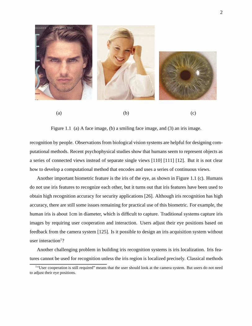
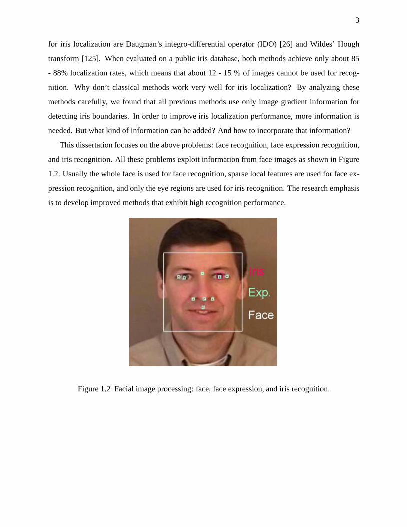


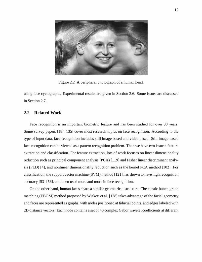


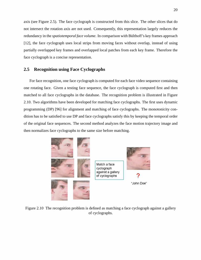


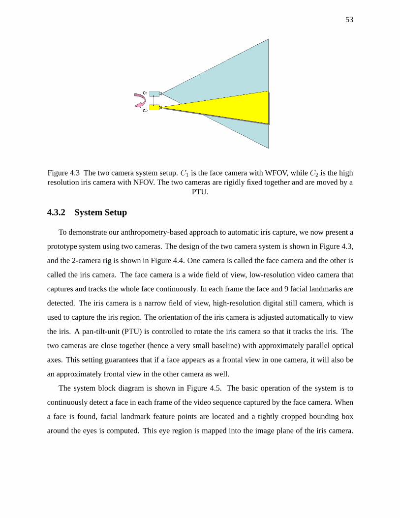
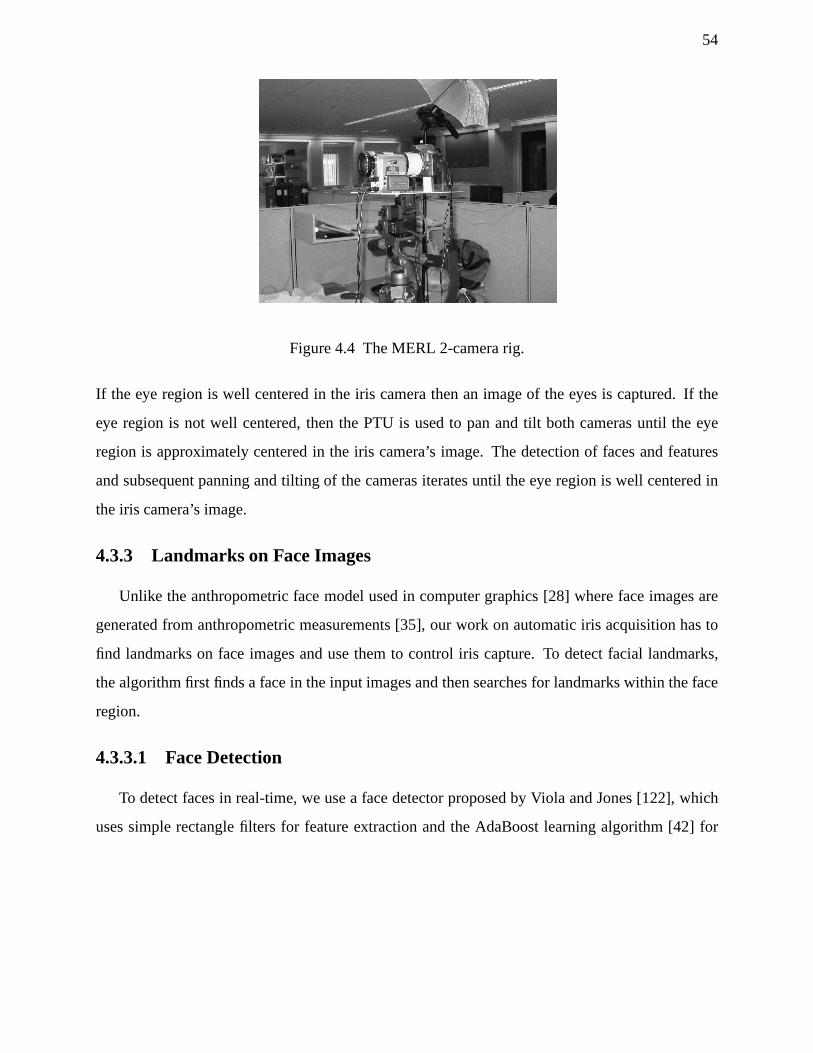

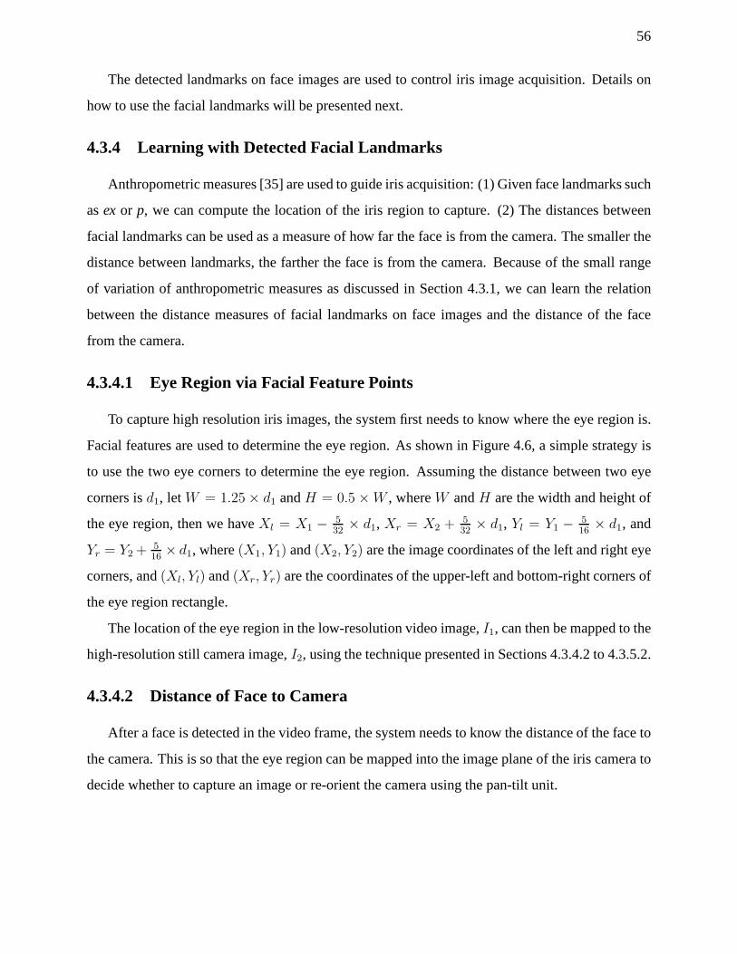


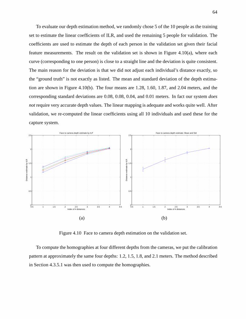


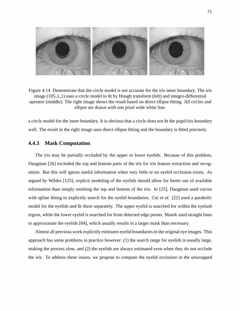


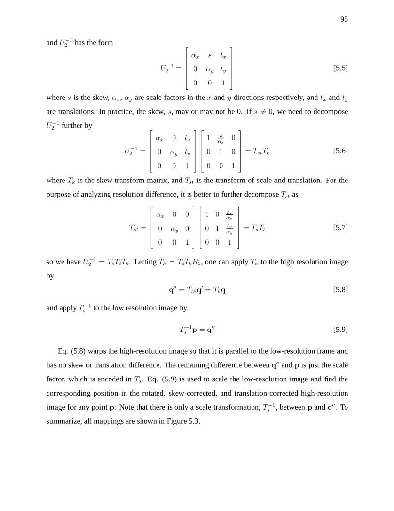


![1992-8645 IMAGE FUSION TECHNIQUES FOR IRIS AND · PDF fileand iris boundary. In iris segmentation the iris ... lower eyelid using the linear Hough transform [13]. In this paper Iris](https://static.documents.pub/doc/80x56/5aac91c37f8b9aa06a8d31f9/1992-8645-image-fusion-techniques-for-iris-and-iris-boundary-in-iris-segmentation.jpg)


