570
Face Recognition

Face Recognition


Face Recognition
Edited by Kresimir Delac and Mislav Grgic
I-TECH Education and Publishing

IV
Published by the I-Tech Education and Publishing, Vienna, Austria
Abstracting and non-profit use of the material is permitted with credit to the source. Statements and opinions expressed in the chapters are these of the individual contributors and not necessarily those of the editors or publisher. No responsibility is accepted for the accuracy of information contained in the published articles. Publisher assumes no responsibility liability for any damage or injury to persons or property arising out of the use of any materials, instructions, methods or ideas contained inside. After this work has been published by the Advanced Robotic Systems International, authors have the right to republish it, in whole or part, in any publication of which they are an author or editor, and the make other personal use of the work.
© 2007 I-Tech Education and Publishing www.ars-journal.com Additional copies can be obtained from: [email protected]
First published June 2007 Printed in Croatia
A catalog record for this book is available from the Austrian Library. Face Recognition, Edited by Kresimir Delac and Mislav Grgic
p. cm. ISBN 3-86611-283-1 1. Face Recognition. 2. Face sinthesys. 3. Applications.

V
Preface
Face recognition is a task humans perform remarkably easily and successfully. This appar-ent simplicity was shown to be dangerously misleading as the automatic face recognition seems to be a problem that is still far from solved. In spite of more than 20 years of extensive research, large number of papers published in journals and conferences dedicated to this area, we still can not claim that artificial systems can measure to human performance. Automatic face recognition is intricate primarily because of difficult imaging conditions (lighting and viewpoint changes induced by body movement) and because of various other effects like aging, facial expressions, occlusions etc. Researchers from computer vision, im-age analysis and processing, pattern recognition, machine learning and other areas are working jointly, motivated largely by a number of possible practical applications. The goal of this book is to give a clear picture of the current state-of-the-art in the field of automatic face recognition across three main areas of interest: biometrics, cognitive models and human-computer interaction. Face recognition has an important advantage over other biomet-ric technologies - it is a nonintrusive and easy to use method. As such, it became one of three identification methods used in e-passports and a biometric of choice for many other security applications. Cognitive and perception models constitute an important platform for inter-disciplinary research, connecting scientists from seemingly incompatible areas and enabling them to exchange methodologies and results on a common problem. Evidence from neuro-biological, psychological, perceptual and cognitive experiments provide potentially useful insights into how our visual system codes, stores and recognizes faces. These insights can then be connected to artificial solutions. On the other hand, it is generally believed that the success or failure of automatic face recognition systems might inform cognitive and percep-tion science community about which models have the potential to be candidates for those used by humans. Making robots and computers more "human" (through human-computer interaction) will improve the quality of human-robot co-existence in the same space and thus alleviate their adoption into our every day lives. In order to achieve this, robots must be able to identify faces, expressions and emotions while interacting with humans. Hopefully, this book will serve as a handbook for students, researchers and practitioners in the area of automatic (computer) face recognition and inspire some future research ideas by identifying potential research directions. The book consists of 28 chapters, each focusing on a certain aspect of the problem. Within every chapter the reader will be given an overview of background information on the subject at hand and in many cases a description of the au-thors' original proposed solution. The chapters in this book are sorted alphabetically, ac-cording to the first author's surname. They should give the reader a general idea where the

VI
current research efforts are heading, both within the face recognition area itself and in inter-disciplinary approaches. Chapter 1 describes a face recognition system based on 3D features, with applications in Ambient Intelligence Environment. The system is placed within a framework of home automation - a community of smart objects powered by high user-friendliness. Chapter 2 addresses one of the most intensely researched problems in face recognition - the problem of achieving illumination invariance. The authors deal with this problem through a novel framework based on simple image filtering techniques. In chapter 3 a novel method for pre-cise automatic localization of certain characteristic points in a face (such as the centers and the corners of the eyes, tip of the nose, etc) is presented. An interesting analysis of the rec-ognition rate as a function of eye localization precision is also given. Chapter 4 gives a de-tailed introduction into wavelets and their application in face recognition as tools for image preprocessing and feature extraction. Chapter 5 reports on an extensive experiment performed in order to analyze the effects of JPEG and JPEG2000 compression on face recognition performance. It is shown that tested recognition methods are remarkably robust to compression, and the conclusions are statisti-cally confirmed using McNemar's hypothesis testing. Chapter 6 introduces a feed-forward neural network architecture combined with PCA and LDA into a novel approach. Chapter 7 addresses the multi-view recognition problem by using a variant of SVM and decomposing the problem into a series of easier two-class problems. Chapter 8 describes three different hardware platforms dedicated to face recognition and brings us one step closer to real-world implementation. In chapter 9 authors combine face and gesture recognition in a human-robot interaction framework. Chapter 10 considers fuzzy-geometric approach and symbolic data analysis for modeling the uncertainty of information about facial features. Chapter 11 reviews some known ap-proaches (e.g. PCA, LDA, LPP, LLE, etc.) and presents a case study of intelligent face recog-nition using global pattern averaging. A theoretical analysis and application suggestion of the compact optical parallel correlator for face recognition is presented in chapter 12. Im-proving the quality of co-existence of humans and robots in the same space through another merge of face and gesture recognition is presented in chapter 13, and spontaneous facial ac-tion recognition is addressed in chapter 14. Based on lessons learned from human visual system research and contrary to traditional practice of focusing recognition on internal face features (eyes, nose, and mouth), in chapter 15 a possibility of using external features (hair, forehead, laterals, ears, jaw line and chin) is explored. In chapter 16 a hierarchical neural network architecture is used to define a com-mon framework for higher level cognitive functions. Simulation is performed indicating that both face recognition and facial expression recognition can be realized efficiently using the presented framework. Chapter 17 gives a detailed mathematical overview of some tradi-tional and modern subspace analysis methods, and chapter 18 reviews in depth some near-est feature classifiers and introduces dissimilarity representations as a recognition tool. In chapter 19 the authors present a security system in which an image of a known person is matched against multiple images extracted from a video fragment of a person approaching a protected entrance Chapter 20 presents recent advances in machine analysis of facial expressions with special attention devoted to several techniques recently proposed by the authors. 3D face recogni-tion is covered in chapter 21. Basic approaches are discussed and an extensive list of refer-

VII
ences is given, making this chapter an ideal starting point for researchers new in the area. After multi-modal human verification system using face and speech is presented in chapter 22, the same authors present a new face detection and recognition method using optimized 3D information from stereo images in chapter 23. Far-field unconstrained video-to-video face recognition system is proposed in chapter 24. Chapter 25 examines the results of research on humans in order to come up with some hints for designs of artificial systems for face recognition. Frequency domain processing and rep-resentation of faces is reviewed in chapter 26 along with a thorough analysis of a family of advanced frequency domain matching algorithms collectively know as the advanced corre-lation filters. Chapter 27 addresses the problem of class-based image synthesis and recogni-tion with varying illumination conditions. Chapter 28 presents a mixed reality virtual sys-tem with a framework of using a stereo video and 3D computer graphics model.
June 2007 Kresimir Delac Mislav Grgic
University of Zagreb Faculty of Electrical Engineering and Computing Department of Wireless Communications Unska 3/XII, HR-10000 Zagreb, Croatia E-mail: [email protected]


IX
Contents
Preface .................................................................................................................................V
1. 3D Face Recognition in a Ambient Intelligence Environment Scenario................. 001
Andrea F. Abate, Stefano Ricciardi and Gabriele Sabatino
2. Achieving Illumination Invariance using Image Filters............................................ 015
Ognjen Arandjelovic and Roberto Cipolla
3. Automatic Facial Feature Extraction for Face Recognition..................................... 031
Paola Campadelli, Raffaella Lanzarotti and Giuseppe Lipori
4. Wavelets and Face Recognition ................................................................................ 059
Dao-Qing Dai and Hong Yan
5. Image Compression Effects in Face Recognition Systems .................................... 075
Kresimir Delac, Mislav Grgic and Sonja Grgic
6. PCA and LDA based Neural Networks for Human Face Recognition..................... 093
Alaa Eleyan and Hasan Demirel
7. Multi-View Face Recognition with Min-Max Modular Support Vector Machines ................................................................................ 107
Zhi-Gang Fan and Bao-Liang Lu
8. Design, Implementation and Evaluation of Hardware Vision Systems dedicated to Real-Time Face Recognition .................................................................... 123
Ginhac Dominique, Yang Fan and Paindavoine Michel
9. Face and Gesture Recognition for Human-Robot Interaction ................................. 149
Md. Hasanuzzaman and Haruki Ueno

X
10. Modelling Uncertainty in Representation of Facial Features for Face Recognition....................................................................................... 183
Hiremath P.S., Ajit Danti and Prabhakar C.J.
11. Intelligent Global Face Recognition ........................................................................ 219
Adnan Khashman
12. Compact Parallel Optical Correlator for Face Recognition and its Application ........................................................................... 235
Kashiko Kodate and Eriko Watanabe
13. Human Detection and Gesture Recognition Based on Ambient Intelligence ...................................................................................... 261
Naoyuki Kubota
14. Investigating Spontaneous Facial Action Recognition through AAM Representations of the Face................................................................... 275
Simon Lucey, Ahmed Bilal Ashraf and Jeffrey F. Cohn
15. Measuring External Face Appearance for Face Classification ............................ 287
David Masip, Agata Lapedriza and Jordi Vitria
16. Selection and Efficient Use of Local Features for Face and Facial Expression Recognition in a Cortical Architecture........................................... 305
Masakazu Matsugu
17. Image-based Subspace Analysis for Face Recognition ........................................ 321
Vo Dinh Minh Nhat and SungYoung Lee
18. Nearest Feature Rules and Dissimilarity Representations for Face Recognition Problems ..................................................................................... 337
Mauricio Orozco-Alzate and German Castellanos-Dominguez
19. Improving Face Recognition by Video Spatial Morphing ...................................... 357
Armando Padilha, Jorge Silva and Raquel Sebastiao
20. Machine Analysis of Facial Expressions ................................................................ 377
Maja Pantic and Marian Stewart Bartlett
21. 3D Face Recognition................................................................................................. 417
Theodoros Papatheodorou and Daniel Rueckert
22. Multi-Modal Human Verification using Face and Speech ...................................... 447
Changhan Park and Joonki Paik

XI
23. Face Recognition Using Optimized 3D Information from Stereo Images .................................................................................... 457
Changhan Park and Joonki Paik
24. Far-Field, Multi-Camera, Video-to-Video Face Recognition .................................. 467
Aristodemos Pnevmatikakis and Lazaros Polymenakos
25. Facing Visual Tasks Based on Different Cognitive Architectures ........................ 487
Marcos Ruiz-Soler and Francesco S. Beltran
26. Frequency Domain Face Recognition ..................................................................... 495
Marios Savvides, Ramamurthy Bhagavatula, Yung-hui Li and Ramzi Abiantun
27. From Canonical Face to Synthesis An Illumination Invariant Face Recognition Approach ................................................ 527
Tele Tan
28. A Feature-level Fusion of Appearance and Passive Depth Information for Face Recognition ........................................................ 537
Jian-Gang Wang, Kar-Ann Toh, Eric Sung and Wei-Yun Yau


1
3D Face Recognition in a Ambient Intelligence Environment Scenario
Andrea F. Abate, Stefano Ricciardi and Gabriele Sabatino Dip. di Matematica e Informatica - Università degli Studi di Salerno
Italy
1. Introduction
Information and Communication Technologies are increasingly entering in all aspects of our life and in all sectors, opening a world of unprecedented scenarios where people interact with electronic devices embedded in environments that are sensitive and responsive to the presence of users. Indeed, since the first examples of “intelligent” buildings featuring computer aided security and fire safety systems, the request for more sophisticated services, provided according to each user’s specific needs has characterized the new tendencies within domotic research. The result of the evolution of the original concept of home automation is known as Ambient Intelligence (Aarts & Marzano, 2003), referring to an environment viewed as a “community” of smart objects powered by computational capability and high user-friendliness, capable of recognizing and responding to the presence of different individuals in a seamless, not-intrusive and often invisible way. As adaptivity here is the key for providing customized services, the role of person sensing and recognition become of fundamental importance. This scenario offers the opportunity to exploit the potential of face as a not intrusive biometric identifier to not just regulate access to the controlled environment but to adapt the provided services to the preferences of the recognized user. Biometric recognition (Maltoni et al., 2003) refers to the use of distinctive physiological (e.g., fingerprints, face, retina, iris) and behavioural (e.g., gait, signature) characteristics, called biometric identifiers, for automatically recognizing individuals. Because biometric identifiers cannot be easily misplaced, forged, or shared, they are considered more reliable for person recognition than traditional token or knowledge-based methods. Others typical objectives of biometric recognition are user convenience (e.g., service access without a Personal Identification Number), better security (e.g., difficult to forge access). All these reasons make biometrics very suited for Ambient Intelligence applications, and this is specially true for a biometric identifier such as face which is one of the most common methods of recognition that humans use in their visual interactions, and allows to recognize the user in a not intrusive way without any physical contact with the sensor. A generic biometric system could operate either in verification or identification modality, better known as one-to-one and one-to-many recognition (Perronnin & Dugelay, 2003). In the proposed Ambient Intelligence application we are interested in one-to-one recognition,

Face Recognition 2
as we want recognize authorized users accessing the controlled environment or requesting a specific service. We present a face recognition system based on 3D features to verify the identity of subjects accessing the controlled Ambient Intelligence Environment and to customize all the services accordingly. In other terms to add a social dimension to man-machine communication and thus may help to make such environments more attractive to the human user. The proposed approach relies on stereoscopic face acquisition and 3D mesh reconstruction to avoid highly expensive and not automated 3D scanning, typically not suited for real time applications. For each subject enrolled, a bidimensional feature descriptor is extracted from its 3D mesh and compared to the previously stored correspondent template. This descriptor is a normal map, namely a color image in which RGB components represent the normals to the face geometry. A weighting mask, automatically generated for each authorized person, improves recognition robustness to a wide range of facial expression. This chapter is organized as follows. In section 2 related works are presented and the proposed method is introduced. In section 3 the proposed face recognition method is presented in detail. In section 4 the Ambient Intelligence framework is briefly discussed and experimental results are shown and commented. The paper concludes in section 5 showing directions for future research and conclusions.
2. Related Works
In their survey on state of the art in 3D and multi-modal face recognition, Bowyer et al. (Bowyer et al., 2004) describe the most recent results and research trends, showing that “the variety and sophistication of algorithmic approaches explored is expanding”. The main challenges in this field result to be the improvement of recognition accuracy, a greater robustness to facial expressions, and, more recently, the efficiency of algorithms. Many methods are based on Principal Component Analysis (PCA), such is the case of Hester et al. (Hester et al., 2003) which tested the potential and the limits of PCA varying the number of eigenvectors and the size of range images. Pan et al. (Pan et al., 2005) apply PCA to a novel mapping of the 3D data to a range, or depth, image, while Xu et al. (Xu et al., 2004) aim to divide face in sub-regions using nose as the anchor, PCA to reduce feature space dimensionality and minimum distance for matching. Another major research trend is based on Iterative Closest Point (ICP) algorithm, which has been exploited in many variations for 3D shape aligning, matching or both. The first example of this kind of approach to face recognition has been presented from Medioni and Waupotitsch (Medioni & Waupotitsch, 2003), then Lu and Jain (Lu & Jain, 2005) developed an extended version aimed to cope with expressive variations, whereas Chang et al. (Chang et al., 2005) proposed to apply ICP not to the whole face but to a set of selected subregions instead. As a real face is fully described by its 3D shape and its texture, it is reasonable to use both kind of data (geometry and color or intensity) to improve recognition reliability: this is the idea behind Multi-Modal or (3D+2D) face recognition. The work by Tsalakanidou et al. (Tsalakanidou et al., 2003) is based on PCA to compare both probe’s range image and intensity/color image to the gallery, Papatheodorou and Rueckert (Papatheodorou & Rueckert, 2004) presented a 4D registration method based on Iterative Closest Point (ICP), augmented with texture data. Bronstein et al. (Bronstein et al., 2003) propose a multi-modal 3D + 2D recognition using eigen decomposition of flattened textures and canonical images. Other authors combine 3D and 2D similarity scores obtained comparing 3D and 2D profiles
3D Face Recognition in a Ambient Intelligence Environment Scenario 3
(Beumier & Acheroy, 2000), or extract a feature vector combining Gabor filter responses in 2D and point signatures in 3D (Wang et al., 2003).
3. Description of Facial Recognition System
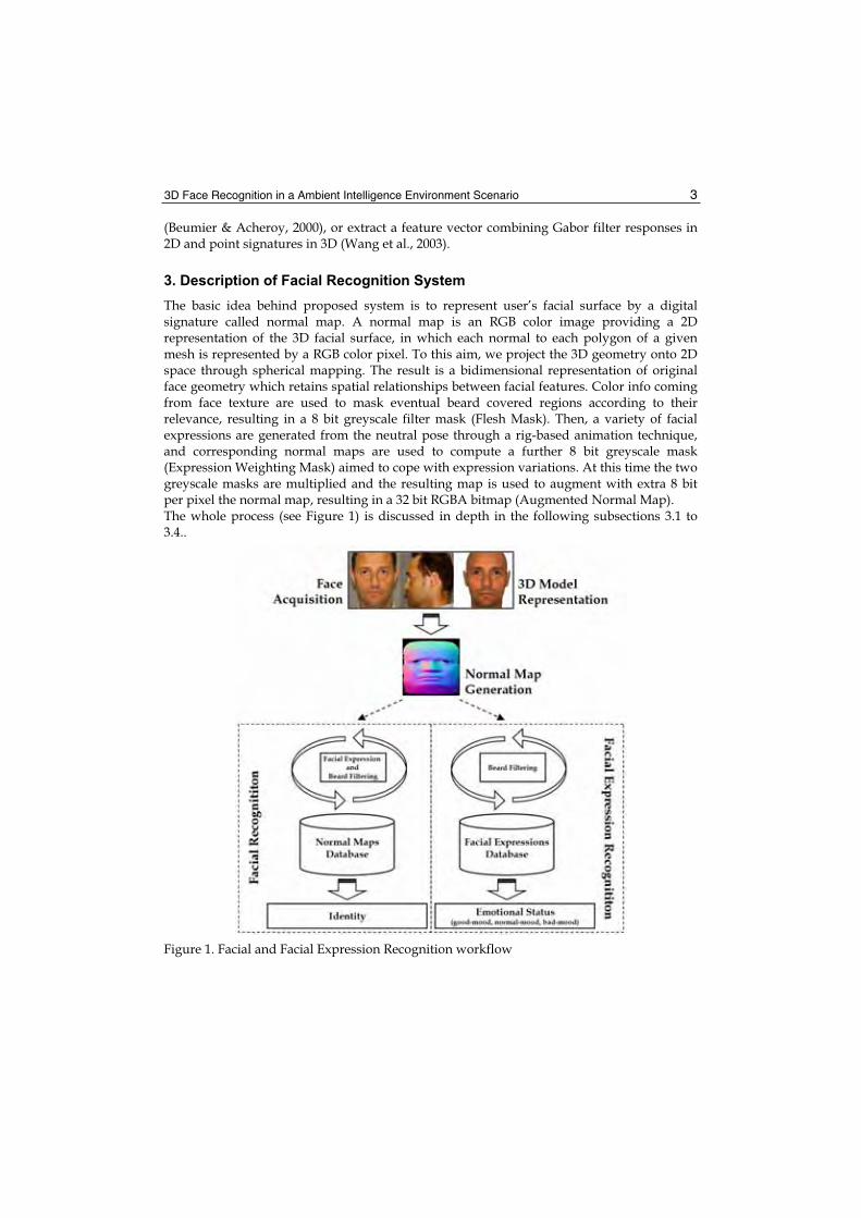
The basic idea behind proposed system is to represent user’s facial surface by a digital signature called normal map. A normal map is an RGB color image providing a 2D representation of the 3D facial surface, in which each normal to each polygon of a given mesh is represented by a RGB color pixel. To this aim, we project the 3D geometry onto 2D space through spherical mapping. The result is a bidimensional representation of original face geometry which retains spatial relationships between facial features. Color info coming from face texture are used to mask eventual beard covered regions according to their relevance, resulting in a 8 bit greyscale filter mask (Flesh Mask). Then, a variety of facial expressions are generated from the neutral pose through a rig-based animation technique, and corresponding normal maps are used to compute a further 8 bit greyscale mask (Expression Weighting Mask) aimed to cope with expression variations. At this time the two greyscale masks are multiplied and the resulting map is used to augment with extra 8 bit per pixel the normal map, resulting in a 32 bit RGBA bitmap (Augmented Normal Map). The whole process (see Figure 1) is discussed in depth in the following subsections 3.1 to 3.4..
Figure 1. Facial and Facial Expression Recognition workflow
Face Recognition 4
3.1 Face Capturing
As the proposed method works on 3D polygonal meshes we firstly need to acquire actual faces and to represent them as polygonal surfaces. The Ambient Intelligence context, in which we are implementing face recognition, requires fast user enrollment to avoid annoying waiting time. Usually, most 3D face recognition methods work on a range image of the face, captured with laser or structured light scanner. This kind of devices offer high resolution in the captured data, but they are too slow for a real time face acquisition. Face unwanted motion during capturing could be another issue, while laser scanning could not be harmless to the eyes. For all this reasons we opted for a 3D mesh reconstruction from stereoscopic images, based on (Enciso et al., 1999) as it requires a simple equipment more likely to be adopted in a real application: a couple of digital cameras shooting at high shutter speed from two slightly different angles with strobe lighting. Though the resulting face shape accuracy is inferior compared to real 3D scanning it proved to be sufficient for recognition yet much faster, with a total time required for mesh reconstruction of about 0.5 sec. on a P4/3.4 Ghz based PC, offering additional advantages, such as precise mesh alignment in 3D space thanks to the warp based approach, facial texture generation from the two captured orthogonal views and its automatic mapping onto the reconstructed face geometry.
3.2 Building a Normal Map
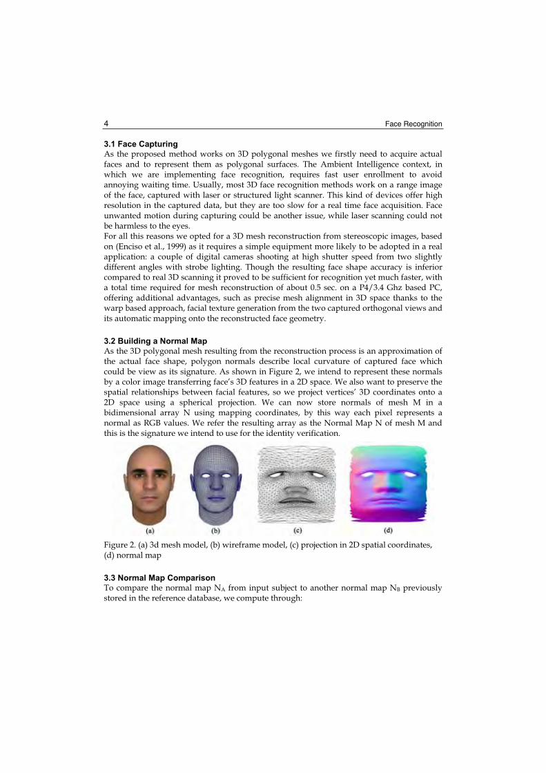
As the 3D polygonal mesh resulting from the reconstruction process is an approximation of the actual face shape, polygon normals describe local curvature of captured face which could be view as its signature. As shown in Figure 2, we intend to represent these normals by a color image transferring face’s 3D features in a 2D space. We also want to preserve the spatial relationships between facial features, so we project vertices’ 3D coordinates onto a 2D space using a spherical projection. We can now store normals of mesh M in a bidimensional array N using mapping coordinates, by this way each pixel represents a normal as RGB values. We refer the resulting array as the Normal Map N of mesh M and this is the signature we intend to use for the identity verification.
Figure 2. (a) 3d mesh model, (b) wireframe model, (c) projection in 2D spatial coordinates, (d) normal map
3.3 Normal Map Comparison
To compare the normal map NA from input subject to another normal map NB previously stored in the reference database, we compute through:
3D Face Recognition in a Ambient Intelligence Environment Scenario 5
( )BABABA NNNNNN bbggrr ⋅+⋅+⋅= arccosθ (1)
the angle included between each pairs of normals represented by colors of pixels with corresponding mapping coordinates, and store it in a new Difference Map D with components r, g and b opportunely normalized from spatia l domain to color domain, so
1,,0 ≤≤AAA NNN bgr and 1,,0 ≤≤
BBB NNN bgr . The value , with 0 < , is the angular
difference between the pixels with coordinates ( )AA NN yx , in NA and ( )
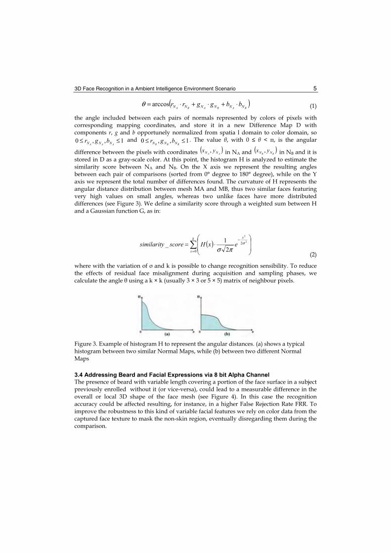
BB NN yx , in NB and it is stored in D as a gray-scale color. At this point, the histogram H is analyzed to estimate the similarity score between NA and NB. On the X axis we represent the resulting angles between each pair of comparisons (sorted from 0° degree to 180° degree), while on the Y axis we represent the total number of differences found. The curvature of H represents the angular distance distribution between mesh MA and MB, thus two similar faces featuring very high values on small angles, whereas two unlike faces have more distributed differences (see Figure 3). We define a similarity score through a weighted sum between H and a Gaussian function G, as in:
( )=
−⋅=
k
x
x
exHscoresimilarity0
2 2
2
2
1_ σ
πσ (2)
where with the variation of and k is possible to change recognition sensibility. To reduce the effects of residual face misalignment during acquisition and sampling phases, we calculate the angle using a k × k (usually 3 × 3 or 5 × 5) matrix of neighbour pixels.
Figure 3. Example of histogram H to represent the angular distances. (a) shows a typical histogram between two similar Normal Maps, while (b) between two different Normal Maps
3.4 Addressing Beard and Facial Expressions via 8 bit Alpha Channel
The presence of beard with variable length covering a portion of the face surface in a subject previously enrolled without it (or vice-versa), could lead to a measurable difference in the overall or local 3D shape of the face mesh (see Figure 4). In this case the recognition accuracy could be affected resulting, for instance, in a higher False Rejection Rate FRR. To improve the robustness to this kind of variable facial features we rely on color data from the captured face texture to mask the non-skin region, eventually disregarding them during the comparison.
Face Recognition 6
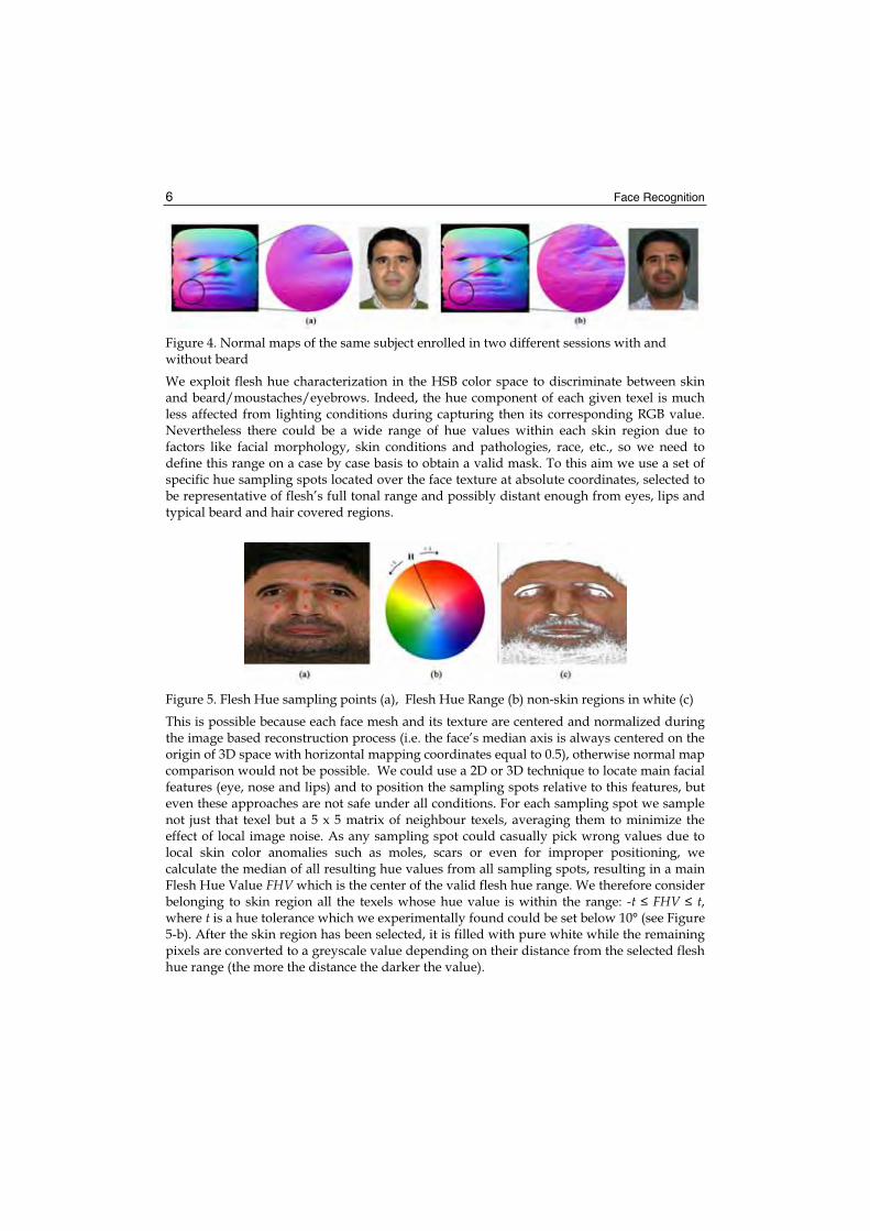
Figure 4. Normal maps of the same subject enrolled in two different sessions with and without beard
We exploit flesh hue characterization in the HSB color space to discriminate between skin and beard/moustaches/eyebrows. Indeed, the hue component of each given texel is much less affected from lighting conditions during capturing then its corresponding RGB value. Nevertheless there could be a wide range of hue values within each skin region due to factors like facial morphology, skin conditions and pathologies, race, etc., so we need to define this range on a case by case basis to obtain a valid mask. To this aim we use a set of specific hue sampling spots located over the face texture at absolute coordinates, selected to be representative of flesh’s full tonal range and possibly distant enough from eyes, lips and typical beard and hair covered regions.
Figure 5. Flesh Hue sampling points (a), Flesh Hue Range (b) non-skin regions in white (c)
This is possible because each face mesh and its texture are centered and normalized during the image based reconstruction process (i.e. the face’s median axis is always centered on the origin of 3D space with horizontal mapping coordinates equal to 0.5), otherwise normal map comparison would not be possible. We could use a 2D or 3D technique to locate main facial features (eye, nose and lips) and to position the sampling spots relative to this features, but even these approaches are not safe under all conditions. For each sampling spot we sample not just that texel but a 5 x 5 matrix of neighbour texels, averaging them to minimize the effect of local image noise. As any sampling spot could casually pick wrong values due to local skin color anomalies such as moles, scars or even for improper positioning, we calculate the median of all resulting hue values from all sampling spots, resulting in a main Flesh Hue Value FHV which is the center of the valid flesh hue range. We therefore consider belonging to skin region all the texels whose hue value is within the range: -t FHV t,where t is a hue tolerance which we experimentally found could be set below 10° (see Figure 5-b). After the skin region has been selected, it is filled with pure white while the remaining pixels are converted to a greyscale value depending on their distance from the selected flesh hue range (the more the distance the darker the value).

3D Face Recognition in a Ambient Intelligence Environment Scenario 7
To improve the facial recognition system and to address facial expressions we opt to the use of expression weighting mask, a subject specific pre-calculated mask aimed to assign different relevance to different face regions. This mask, which shares the same size of normal map and difference map, contains for each pixel an 8 bit weight encoding the local rigidity of the face surface based on the analysis of a pre-built set of facial expressions of the same subject. Indeed, for each subject enrolled, each of expression variations (see Figure 6) is compared to the neutral face resulting in difference maps.
Figure 6. An example of normal maps of the same subject featuring a neutral pose (leftmost face) and different facial expressions
The average of this set of difference maps specific to the same individual represent its expression weighting mask. More precisely, given a generic face with its normal map N0
(neutral face) and the set of normal maps N1, N2, …, Nn (the expression variations), we first calculate the set of difference map D1, D2, …, Dn resulting from {N0 - N1, N0 - N2, …, N0 – Nn}. The average of set {D1, D2, …, Dn} is the expression weighting mask which is multiplied by the difference map in each comparison between two faces. We generate the expression variations through a parametric rig based deformation system previously applied to a prototype face mesh, morphed to fit the reconstructed face mesh (Enciso et al., 1999). This fitting is achieved via a landmark-based volume morphing where the transformation and deformation of the prototype mesh is guided by the interpolation of a set of landmark points with a radial basis function. To improve the accuracy of this rough mesh fitting we need a surface optimization obtained minimizing a cost function based on the Euclidean distance between vertices. So we can augment each 24 bit normal map with the product of Flesh Mask and Expression Weighting Mask normalized to 8 bit (see Figure 7). The resulting 32 bit per pixel RGBA bitmap can be conveniently managed via various image formats like the Portable Network Graphics format (PNG) which is typically used to store for each pixel 24 bit of colour and 8 bit of alpha channel (transparency). When comparing any two faces, the difference map is computed on the first 24 bit of color info (normals) and multiplied to the alpha channel (filtering mask).
4. Testing Face Recognition System into an Ambient Intelligence Framework
Ambient Intelligence (AmI) worlds offer exciting potential for rich interactive experiences. The metaphor of AmI envisages the future as intelligent environments where humans are surrounded by smart devices that makes the ambient itself perceptive to humans’ needs or wishes. The Ambient Intelligence Environment can be defined as the set of actuators and sensors composing the system together with the domotic interconnection protocol. People interact with electronic devices embedded in environments that are sensitive and responsive to the presence of users. This objective is achievable if the environment is capable to learn,
Face Recognition 8
build and manipulate user profiles considering from a side the need to clearly identify the human attitude; in other terms, on the basis of physical and emotional user status captured from a set of biometric features.
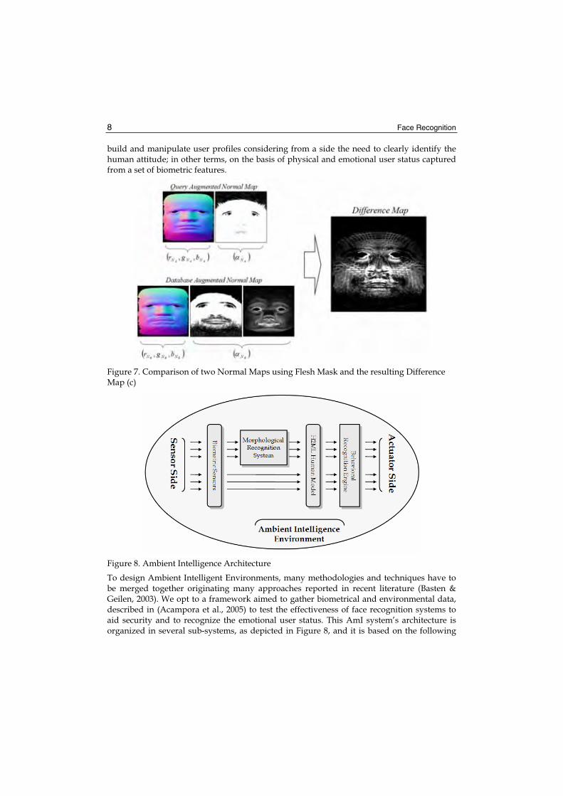
Figure 7. Comparison of two Normal Maps using Flesh Mask and the resulting Difference Map (c)
Figure 8. Ambient Intelligence Architecture
To design Ambient Intelligent Environments, many methodologies and techniques have to be merged together originating many approaches reported in recent literature (Basten & Geilen, 2003). We opt to a framework aimed to gather biometrical and environmental data, described in (Acampora et al., 2005) to test the effectiveness of face recognition systems to aid security and to recognize the emotional user status. This AmI system’s architecture is organized in several sub-systems, as depicted in Figure 8, and it is based on the following

3D Face Recognition in a Ambient Intelligence Environment Scenario 9
sensors and actuators: internal and external temperature sensors and internal temperature actuator, internal and external luminosity sensor and internal luminosity actuator, indoor presence sensor, a infrared camera to capture thermal images of user and a set of color cameras to capture information about gait and facial features. Firstly Biometric Sensors are used to gather user’s biometrics (temperature, gait, position, facial expression, etc.) and part of this information is handled by Morphological Recognition Subsystems (MRS) able to organize it semantically. The resulting description, together with the remaining biometrics previously captured, are organized in a hierarchical structure based on XML technology in order to create a new markup language, called H2ML (Human to Markup Language)representing user status at a given time. Considering a sequence of H2ML descriptions, the Behavioral Recognition Engine (BRE), tries to recognize a particular user behaviour for which the system is able to provide suitable services. The available services are regulated by means of the Service Regulation System (SRS), an array of fuzzy controllers coded in FML (Acampora & Loia, 2004) aimed to achieve hardware transparency and to minimize the fuzzy inference time.This architecture is able to distribute personalized services on the basis of physical and emotional user status captured from a set of biometric features and modelled by means of a mark-up language, based on XML. This approach is particularly suited to exploit biometric technologies to capture user’s physical info gathered in a semantic representation describing a human in terms of morphological features.
4.1 Experimental Results
As one of the aims in experiments was to test the performance of the proposed method in a realistic operative environment, we decided to build a 3D face database from the face capture station used in the domotic system described above. The capture station featured two digital cameras with external electronic strobes shooting simultaneously with a shutter speed of 1/250 sec. while the subject was looking at a blinking led to reduce posing issues. More precisely, every face model in the gallery has been created deforming a pre-aligned prototype polygonal face mesh to closely fit a set of facial features extracted from front and side images of each individual enrolled in the system. Indeed, for each enrolled subject a set of corresponding facial features extracted by a structured snake method from the two orthogonal views are correlated first and then used to guide the prototype mesh warping, performed through a Dirichlet Free Form Deformation. The two captured face images are aligned, combined and blended resulting in a color texture precisely fitting the reconstructed face mesh through the feature points previously extracted. The prototype face mesh used in the dataset has about 7K triangular facets, and even if it is possible to use mesh with higher level of detail we found this resolution to be adequate for face recognition. This is mainly due to the optimized tessellation which privileges key area such as eyes, nose and lips whereas a typical mesh produced by 3D scanner features almost evenly spaced vertices. Another remarkable advantage involved in the warp based mesh generation is the ability to reproduce a broad range of face variations through a rig based deformation system. This technique is commonly used in computer graphics for facial animation (Lee et al., 1995, Blanz & Vetter, 1999) and is easily applied to the prototype mesh linking the rig system to specific subsets of vertices on the face surface. Any facial expression could be mimicked opportunely combining the effect of the rig controlling lips, mouth shape, eye closing or opening, nose
Face Recognition 10
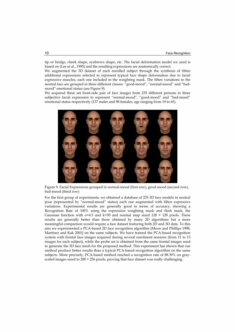
tip or bridge, cheek shape, eyebrows shape, etc. The facial deformation model we used is based on (Lee et al., 1995) and the resulting expressions are anatomically correct. We augmented the 3D dataset of each enrolled subject through the synthesis of fiften additional expressions selected to represent typical face shape deformation due to facial expressive muscles, each one included in the weighting mask. The fiften variations to the neutral face are grouped in three different classes: “good-mood”, “normal-mood” and “bad-mood” emotional status (see Figure 9). We acquired three set front-side pair of face images from 235 different persons in three subjective facial expression to represent “normal-mood”, “good-mood” and “bad-mood” emotional status respectively (137 males and 98 females, age ranging from 19 to 65).
Figure 9. Facial Expressions grouped in normal-mood (first row), good-mood (second row), bad-mood (third row)
For the first group of experiments, we obtained a database of 235 3D face models in neutral pose (represented by “normal-mood” status) each one augmented with fiften expressive variations. Experimental results are generally good in terms of accuracy, showing a Recognition Rate of 100% using the expression weighting mask and flesh mask, the Gaussian function with =4.5 and k=50 and normal map sized 128 × 128 pixels. These results are generally better than those obtained by many 2D algorithms but a more meaningful comparison would require a face dataset featuring both 2D and 3D data. To this aim we experimented a PCA-based 2D face recognition algorithm [Moon and Phillips 1998, Martinez and Kak 2001] on the same subjects. We have trained the PCA-based recognition system with frontal face images acquired during several enrolment sessions (from 11 to 13 images for each subject), while the probe set is obtained from the same frontal images used to generate the 3D face mesh for the proposed method. This experiment has shown that our method produce better results than a typical PCA-based recognition algorithm on the same subjects. More precisely, PCA-based method reached a recognition rate of 88.39% on gray-scaled images sized to 200 × 256 pixels, proving that face dataset was really challenging.

3D Face Recognition in a Ambient Intelligence Environment Scenario 11
0,7
0,75
0,8
0,85
0,9
0,95
1
0,1 0,2 0,3 0,4 0,5 0,6 0,7 0,8 0,9 1
Precision
Recall
only Normal Map
with Expression Weighting Mask
0,7
0,75
0,8
0,85
0,9
0,95
1
0,1 0,2 0,3 0,4 0,5 0,6 0,7 0,8 0,9 1
Precision
Recall
only Normal Map
with Flesh Mask
0,7
0,75
0,8
0,85
0,9
0,95
1
0,1 0,2 0,3 0,4 0,5 0,6 0,7 0,8 0,9 1
Precision
Recall
only Normal Map
with E.W. Mask & Flesh Mask
Figure 10. Precision/Recall Testing with and without Expression Weighting Mask and Flesh Mask to show efficacy respectively to (a) expression variations, (b) beard presence and (c) both
Figure 10 shows the precision/recall improvement provided by the expression weighting mask and flesh mask. The results showed in Figure 10-a were achieved comparing in one-to-many modality a query set with one expressive variations to an answer set composed by one neutral face plus ten expression variations and one face with beard. In Figure 10-b are shown the results of one-to-many comparison between subject with beard and an answer set

Face Recognition 12
composed of one neutral face and ten expressive variations. Finally for the test reported in Figure 10-c the query was an expression variation or a face with beard, while the answer set could contain a neutral face plus ten associated expressive variations or a face with beard. The three charts clearly show the benefits involved with the use of both expressive and flesh mask, specially when combined together. The second group of experiments has been conducted on FRGC dataset rel. 2/Experiment 3s (only shape considered) to test the method's performance with respect to Receiver Operating Characteristic (ROC) curve which plots the False Acceptance Rate (FAR) against Verification Rate (1 – False Rejection Rate or FRR) for various decision thresholds. The 4007 faces provided in the dataset have undergone a pre-processing stage to allow our method to work effectively. The typical workflow included: mesh alignment using the embedded info provided by FRGC dataset such as outer eye corners, nose tip, chin prominence; mesh subsampling to one fourth or original resolution; mesh cropping to eliminate unwanted detail (hair, neck, ears, etc.); normal map filtering by a 5 × 5 median filter to reduce capture noise and artifacts. Fig. 11 shows resulting ROC curves with typical ROC values at FAR = 0.001. The Equal Error Rate (EER) measured on all two galleries reaches 5.45% on the our gallery and 6.55% on FRGC dataset.
Figure 11. Comparison of ROC curves and Verification Rate at FAR=0.001
Finally, we have tested the method in order to evaluate statistically the behaviour of method to recognize the “emotional” status of the user. To this aim, we have performed a one-to-one comparison of a probe set of 3D face models representing real subjective mood status captured by camera (three facial expressions per person) with three gallery set of artificial mood status generated automatically by control rig based deformation system (fifteen facial expression per person grouped as shown in Figure 9). As shown in Table 1, the results are very interesting, because the mean recognition rate on “good-mood” status gallery is 100% while on “normal-mood” and “bad-mood” status galleries is 98.3% and 97.8% respectively

3D Face Recognition in a Ambient Intelligence Environment Scenario 13
(probably, because of the propensity of the people to make similar facial expressions for “normal-mood” and “bad-mood” status).
Recognition Rate “normal-mood” “good-mood” “bad-mood” 98.3% 100% 97.8%
Table 1. The behaviour of method to recognize the “emotional” status of the user
5. Conclusion
We presented a 3D face recognition method applied to an Ambient Intelligence Environment. The proposed approach to acquisition and recognition proved to be suited to the applicative context thanks to high accuracy and recognition speed, effectively exploiting the advantages of face over other biometrics. As the acquisition system requires the user to look at a specific target to allow a valid face capture, we are working on a multi-angle stereoscopic camera arrangement, to make this critical task less annoying and more robust to a wide posing range. This 3D face recognition method based on 3D geometry and color texture is aimed to improve robustness to presence/absence of beard and to expressive variations. It proved to be simple and fast and experiments conducted showed high average recognition rate and a measurable effectiveness of both flesh mask and expression weighting mask. Ongoing research will implement a true multi-modal version of the basic algorithm with a second recognition engine dedicated to the color info (texture) which could further enhance the discriminating power.
6. References
Aarts, E. & Marzano, S. (2003). The New Everyday: Visions of Ambient Intelligence, 010 Publishing, Rotterdam, The Netherlands
Acampora, G. & Loia, V. (2004). Fuzzy Control Interoperability for Adaptive Domotic Framework, Proceedings of 2nd IEEE International Conference on Industrial Informatics,(INDIN04), pp. 184-189, 24-26 June 2004, Berlin, Germany
Acampora, G.; Loia, V.; Nappi, M. & Ricciardi, S. (2005). Human-Based Models for Smart Devices in Ambient Intelligence, Proceedings of the IEEE International Symposium on Industrial Electronics. ISIE 2005. pp. 107- 112, June 20-23, 2005.
Basten, T. & Geilen, M. (2003). Ambient Intelligence: Impact on Embedded System Design, H. de Groot (Eds.), Kluwer Academic Pub., 2003
Beumier, C. & Acheroy, M. (2000). Automatic Face verification from 3D and grey level cues, Proceeding of 11th Portuguese Conference on Pattern Recognition (RECPAD 2000), May 2000, Porto, Portugal.
Blanz, V. & Vetter, T. (1999). A morphable model for the synthesis of 3D faces, Proceedings of SIGGRAPH 99, Los Angeles, CA, ACM, pp. 187-194, Aug. 1999
Bronstein, A.M.; Bronstein, M.M. & Kimmel, R. (2003). Expression-invariant 3D face recognition, Proceedings of Audio and Video-Based Person Authentication (AVBPA 2003), LCNS 2688, J. Kittler and M.S. Nixon, 62-70,2003.

Face Recognition 14
Bowyer, K.W.; Chang, K. & Flynn P.A. (2004). Survey of 3D and Multi-Modal 3D+2D Face Recognition, Proceeding of International Conference on Pattern Recognition, ICPR, 2004
Chang, K.I.; Bowyer, K. & Flynn, P. (2003). Face Recognition Using 2D and 3D Facial Data, Proceedings of the ACM Workshop on Multimodal User Authentication, pp. 25-32, December 2003.
Chang, K.I.; Bowyer, K.W. & Flynn, P.J. (2005). Adaptive rigid multi-region selection for handling expression variation in 3D face recognition, Proceedings of IEEE Workshop on Face Recognition Grand Challenge Experiments, June 2005.
Enciso, R.; Li, J.; Fidaleo, D.A.; Kim, T-Y; Noh, J-Y & Neumann, U. (1999). Synthesis of 3D Faces, Proceeding of International Workshop on Digital and Computational Video,DCV'99, December 1999
Hester, C.; Srivastava, A. & Erlebacher, G. (2003) A novel technique for face recognition using range images, Proceedings of Seventh Int'l Symposium on Signal Processing and Its Applications, 2003.
Lee, Y.; D. Terzopoulos, D. & Waters, K. (1995). Realistic modeling for facial animation, Proceedings of SIGGRAPH 95, Los Angeles, CA, ACM, pp. 55-62, Aug. 1995
Maltoni, D.; Maio D., Jain A.K. & Prabhakar S. (2003). Handbook of Fingerprint Recognition,Springer, New York
Medioni,G. & Waupotitsch R. (2003). Face recognition and modeling in 3D. Prooceding of IEEE International Workshop on Analysis and Modeling of Faces and Gestures (AMFG 2003), pages 232-233, October 2003.
Pan, G.; Han, S.; Wu, Z. & Wang, Y. (2005). 3D face recognition using mapped depth images, Proceedings of IEEE Workshop on Face Recognition Grand Challenge Experiments, June 2005.
Papatheodorou, T. & Rueckert, D. (2004). Evaluation of Automatic 4D Face Recognition Using Surface and Texture Registration, Proceedings of the Sixth IEEE International Conference on Automatic Face and Gesture Recognition, pp. 321-326, May 2004, Seoul, Korea.
Perronnin, G. & Dugelay, J.L. (2003). An Introduction to biometrics and face recognition, Proceedings of IMAGE 2003: Learning, Understanding, Information Retrieval, Medical,Cagliari, Italy, June 2003
Tsalakanidou, F.; Tzovaras, D. & Strintzis, M. G. (2003). Use of depth and color eigenfaces for face recognition, Pattern Recognition Letters, vol. 24, No. 9-10, pp. 1427-1435, Jan-2003.
Xu, C.; Wang, Y.; Tan, t. & Quan, L. (2004). Automatic 3D face recognition combining global geometric features with local shape variation information, Proceedings of Sixth International Conference on Automated Face and Gesture Recognition, May 2004, pp. 308–313.
Wang, Y.; Chua, C. & Ho, Y. (2002). Facial feature detection and face recognition from 2D and 3D images, Pattern Recognition Letters, 23:1191-1202, 2002.

2
Achieving Illumination Invariance using Image Filters
Ognjen Arandjelovi and Roberto Cipolla Department of Engineering, University of Cambridge
UK
1. Introduction
In this chapter we are interested in accurately recognizing human faces in the presence of large and unpredictable illumination changes. Our aim is to do this in a setup realistic for most practical applications, that is, without overly constraining the conditions in which image data is acquired. Specifically, this means that people's motion and head poses are largely uncontrolled, the amount of available training data is limited to a single short sequence per person, and image quality is low. In conditions such as these, invariance to changing lighting is perhaps the most significant practical challenge for face recognition algorithms. The illumination setup in which recognition is performed is in most cases impractical to control, its physics difficult to accurately model and face appearance differences due to changing illumination are often larger than those differences between individuals [1]. Additionally, the nature of most real-world applications is such that prompt, often real-time system response is needed, demanding appropriately efficient as well as robust matching algorithms. In this chapter we describe a novel framework for rapid recognition under varying illumination, based on simple image filtering techniques. The framework is very general and we demonstrate that it offers a dramatic performance improvement when used with a wide range of filters and different baseline matching algorithms, without sacrificing their computational efficiency.
1.1 Previous work and its limitations
The choice of representation, that is, the model used to describe a person's face is central to the problem of automatic face recognition. Consider the components of a generic face recognition system schematically shown in Figure 1. A number of approaches in the literature use relatively complex facial and scene models that explicitly separate extrinsic and intrinsic variables which affect appearance. In most cases, the complexity of these models makes it impossible to compute model parameters as a closed-form expression ("Model parameter recovery" in Figure 1). Rather, model fitting is performed through an iterative optimization scheme. In the 3D Morphable Model of Blanz and Vetter [7], for example, the shape and texture of a novel face are recovered through gradient descent by minimizing the discrepancy between the observed and predicted appearance. Similarly, in Elastic Bunch Graph Matching [8, 23], gradient descent is used to

Face Recognition 16
recover the placements of fiducial features, corresponding to bunch graph nodes and the locations of local texture descriptors. In contrast, the Generic Shape-Illumination Manifold method uses a genetic algorithm to perform a manifold-to-manifold mapping that preserves pose.
Figure 1. A diagram of the main components of a generic face recognition system. The "Model parameter recovery" and "Classification" stages can be seen as mutually complementary: (i) a complex model that explicitly separates extrinsic and intrinsic appearance variables places most of the workload on the former stage, while the classification of the representation becomes straightforward; in contrast, (ii) simplistic models have to resort to more statistically sophisticated approaches to matching
Figure 2. (a) The simplest generative model used for face recognition: images are assumed to consist of the low-frequency band that mainly corresponds to illumination changes, midfrequency band which contains most of the discriminative, personal information and white noise, (b) The results of several most popular image filters operating under the assumption of the frequency model

Achieving Illumination Invariance using Image Filters 17
One of the main limitations of this group of methods arises due to the existence of local minima, of which there are usually many. The key problem is that if the fitted model parameters correspond to a local minimum, classification is performed not merely on noise-contaminated but rather entirely incorrect data. An additional unappealing feature of these methods is that it is also not possible to determine if model fitting failed in such a manner. The alternative approach is to employ a simple face appearance model and put greater emphasis on the classification stage. This general direction has several advantages which make it attractive from a practical standpoint. Firstly, model parameter estimation can now be performed as a closed-form computation, which is not only more efficient, but also void of the issue of fitting failure such that can happen in an iterative optimization scheme. This allows for more powerful statistical classification, thus clearly separating well understood and explicitly modelled stages in the image formation process, and those that are more easily learnt implicitly from training exemplars. This is the methodology followed in this chapter. The sections that follow describe the method in detail, followed by a report of experimental results.
2. Method details
2.1 Image processing filters
Most relevant to the material presented in this chapter are illumination-normalization methods that can be broadly described as quasi illumination-invariant image filters. Theseinclude high-pass [5] and locally-scaled high-pass filters [21], directional derivatives [1, 10, 13, 18], Laplacian-of-Gaussian filters [1], region-based gamma intensity correction filters [2,17] and edge-maps [1], to name a few. These are most commonly based on very simple image formation models, for example modelling illumination as a spatially low-frequency band of the Fourier spectrum and identity-based information as high-frequency [5,11], see Figure 2. Methods of this group can be applied in a straightforward manner to either single or multiple-image face recognition and are often extremely efficient. However, due to the simplistic nature of the underlying models, in general they do not perform well in the presence of extreme illumination changes.
2.2 Adapting to data acquisition conditions
The framework proposed in this chapter is motivated by our previous research and the findings first published in [3]. Four face recognition algorithms, the Generic Shape-Illumination method [3], the Constrained Mutual Subspace Method [12], the commercial system Facelt and a Kullback-Leibler Divergence-based matching method, were evaluated on a large database using (i) raw greyscale imagery, (ii) high-pass (HP) filtered imagery and (iii) the Self-Quotient Image (QI) representation [21]. Both the high-pass and even further Self Quotient Image representations produced an improvement in recognition for all methods over raw grayscale, as shown in Figure 3, which is consistent with previous findings in the literature [1,5,11,21]. Of importance to this work is that it was also examined in which cases these filters help and how much depending on the data acquisition conditions. It was found that recognition rates using greyscale and either the HP or the QI filter negatively correlated (with p -0.7), as illustrated in Figure 4. This finding was observed consistently across the result of the four algorithms, all of which employ mutually drastically different underlying models.
Face Recognition 18
a) b)
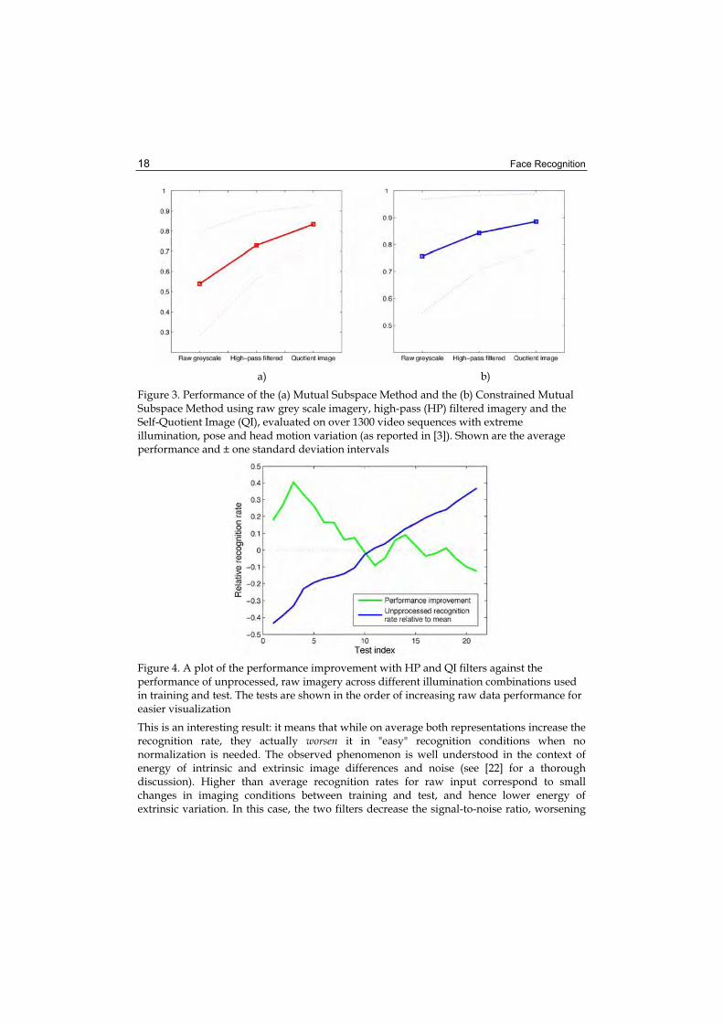
Figure 3. Performance of the (a) Mutual Subspace Method and the (b) Constrained Mutual Subspace Method using raw grey scale imagery, high-pass (HP) filtered imagery and the Self-Quotient Image (QI), evaluated on over 1300 video sequences with extreme illumination, pose and head motion variation (as reported in [3]). Shown are the average performance and ± one standard deviation intervals
Figure 4. A plot of the performance improvement with HP and QI filters against the performance of unprocessed, raw imagery across different illumination combinations used in training and test. The tests are shown in the order of increasing raw data performance for easier visualization
This is an interesting result: it means that while on average both representations increase the recognition rate, they actually worsen it in "easy" recognition conditions when no normalization is needed. The observed phenomenon is well understood in the context of energy of intrinsic and extrinsic image differences and noise (see [22] for a thorough discussion). Higher than average recognition rates for raw input correspond to small changes in imaging conditions between training and test, and hence lower energy of extrinsic variation. In this case, the two filters decrease the signal-to-noise ratio, worsening
Achieving Illumination Invariance using Image Filters 19
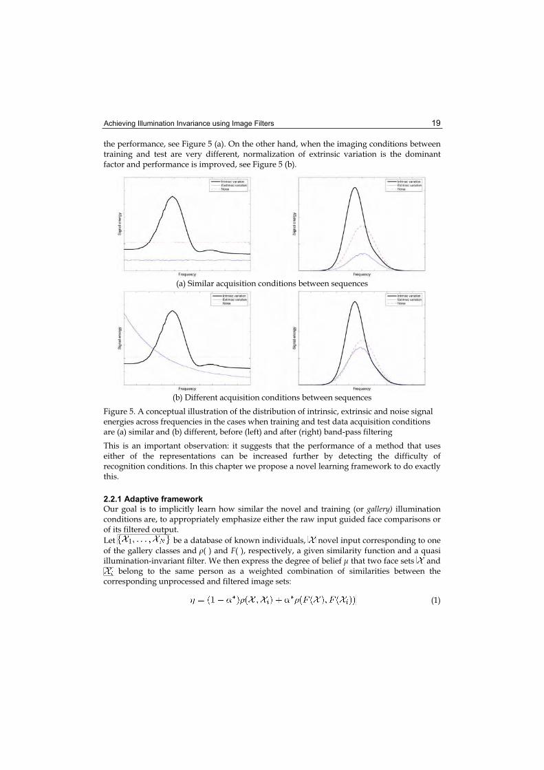
the performance, see Figure 5 (a). On the other hand, when the imaging conditions between training and test are very different, normalization of extrinsic variation is the dominant factor and performance is improved, see Figure 5 (b).
(a) Similar acquisition conditions between sequences
(b) Different acquisition conditions between sequences
Figure 5. A conceptual illustration of the distribution of intrinsic, extrinsic and noise signal energies across frequencies in the cases when training and test data acquisition conditions are (a) similar and (b) different, before (left) and after (right) band-pass filtering
This is an important observation: it suggests that the performance of a method that uses either of the representations can be increased further by detecting the difficulty of recognition conditions. In this chapter we propose a novel learning framework to do exactly this.
2.2.1 Adaptive framework
Our goal is to implicitly learn how similar the novel and training (or gallery) illumination conditions are, to appropriately emphasize either the raw input guided face comparisons or of its filtered output. Let be a database of known individuals, novel input corresponding to one of the gallery classes and ( ) and F( ), respectively, a given similarity function and a quasi illumination-invariant filter. We then express the degree of belief μ that two face sets and
belong to the same person as a weighted combination of similarities between the corresponding unprocessed and filtered image sets:
(1)
Face Recognition 20
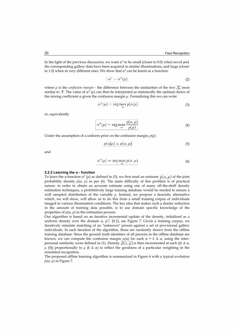
In the light of the previous discussion, we want * to be small (closer to 0.0) when novel and the corresponding gallery data have been acquired in similar illuminations, and large (closer to 1.0) when in very different ones. We show that * can be learnt as a function:
(2)
where μ is the confusion margin - the difference between the similarities of the two most similar to . The value of * (μ) can then be interpreted as statistically the optimal choice of the mixing coefficient given the confusion margin μ. Formalizing this we can write
(3)
or, equivalently
(4)
Under the assumption of a uniform prior on the confusion margin, p(μ)
(5)
and
(6)
2.2.2 Learning the - function
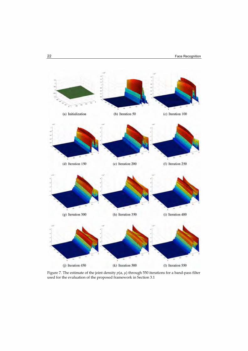
To learn the a-function * (μ) as defined in (3), we first need an estimate of the joint probability density p( , μ) as per (6). The main difficulty of this problem is of practical nature: in order to obtain an accurate estimate using one of many off-the-shelf density estimation techniques, a prohibitively large training database would be needed to ensure a well sampled distribution of the variable μ. Instead, we propose a heuristic alternative which, we will show, will allow us to do this from a small training corpus of individuals imaged in various illumination conditions. The key idea that makes such a drastic reduction in the amount of training data possible, is to use domain specific knowledge of the properties of p( , μ) in the estimation process. Our algorithm is based on an iterative incremental update of the density, initialized as a uniform density over the domain , μ [0,1], see Figure 7. Given a training corpus, we iteratively simulate matching of an "unknown" person against a set of provisional gallery individuals. In each iteration of the algorithm, these are randomly drawn from the offline training database. Since the ground truth identities of all persons in the offline database are known, we can compute the confusion margin μ( ) for each = k , using the inter-personal similarity score defined in (1). Density is then incremented at each ((k ,μ (0)) proportionally to μ (k ) to reflect the goodness of a particular weighting in the simulated recognition.The proposed offline learning algorithm is summarized in Figure 6 with a typical evolution p( , μ) in Figure 7.

Achieving Illumination Invariance using Image Filters 21
The final stage of the offline learning in our method involves imposing the monotonicity constraint on * (μ) and smoothing of the result, see Figure 8.
3. Empirical evaluation
To test the effectiveness of the described recognition framework, we evaluated its perfor-mance on 1662 face motion video sequences from four databases:
Figure 6. Offline training algorithm
Face Recognition 22
Figure 7. The estimate of the joint density p( , μ) through 550 iterations for a band-pass filter used for the evaluation of the proposed framework in Section 3.1

Achieving Illumination Invariance using Image Filters 23
Figure 8. Typical estimates of the -function plotted against confusion margin μ. The estimate shown was computed using 40 individuals in 5 illumination conditions for a Gaussian high-pass filter. As expected, * assumes low values for small confusion margins and high values for large confusion margins (see (1))
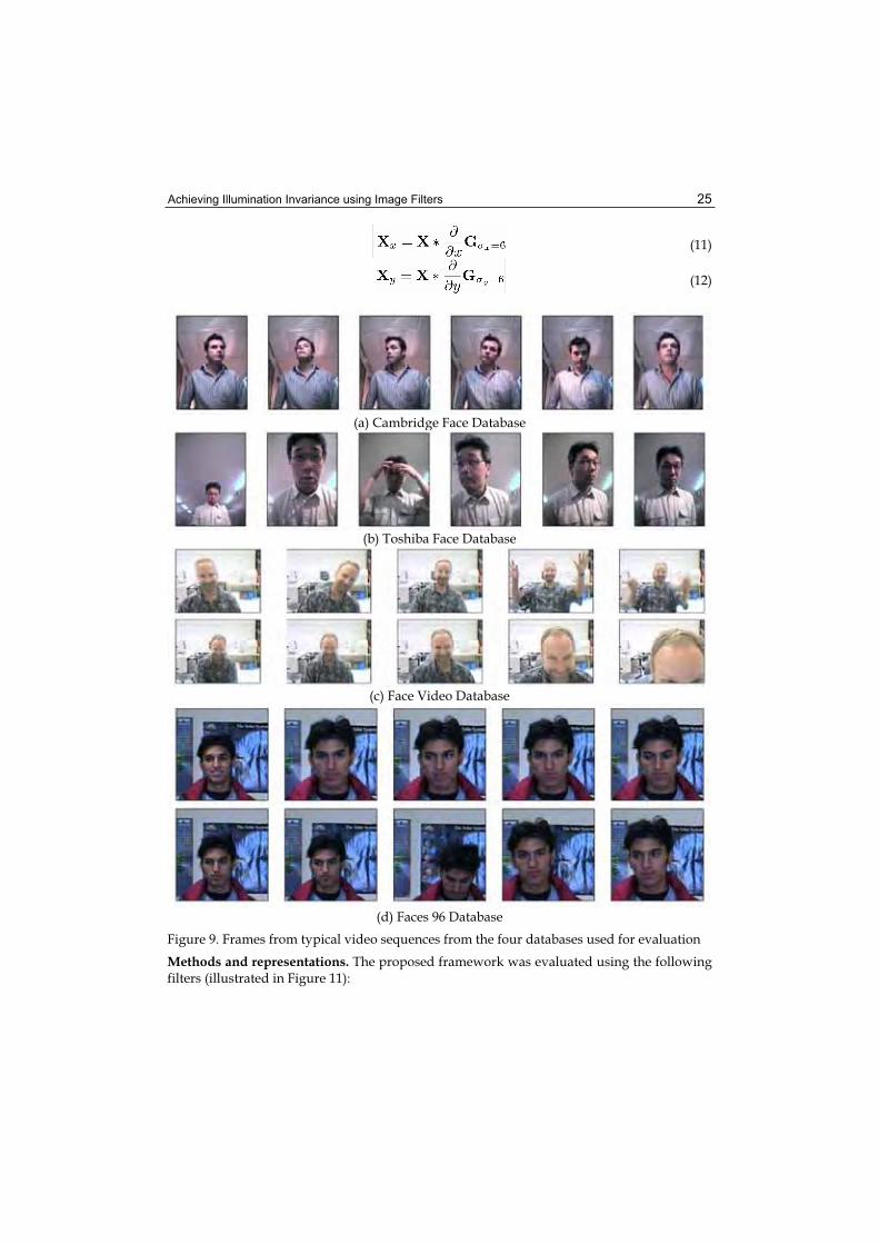
CamFace with 100 individuals of varying age and ethnicity, and equally represented genders. For each person in the database we collected 7 video sequences of the person in arbitrary motion (significant translation, yaw and pitch, negligible roll), each in a different illumination setting, see Figure 9 (a) and 10, at l0 fps and 320 x 240 pixel resolution (face size 60 pixels) 1.
ToshFace kindly provided to us by Toshiba Corp. This database contains 60 individuals of varying age, mostly male Japanese, and 10 sequences per person. Each sequence corresponds to a different illumination setting, at l0 fps and 320 x 240 pixel resolution (face size 60 pixels), see Figure 9 (b).
Face Video freely available2 and described in [14]. Briefly, it contains 11 individuals and 2 sequences per person, little variation in illumination, but extreme and uncontrolled
1 A thorough description of the University of Cambridge face database with examples of video sequences is available at http: //mi.eng.cam. ac.uk/~oa214/.2 See http: / /synapse. vit. lit. nrc. ca/db/video/ faces /cvglab.

Face Recognition 24
variations in pose and motion, acquired at 25fps and 160 x 120 pixel resolution (face size 45 pixels), see Figure 9 (c).
Faces96 the most challenging subset of the University of Essex face database, freely available from http://cswww.essex.ac.uk/mv/allfaces/ faces96 .html. It contains 152 individuals, most 18-20 years old and a single 20-frame sequence per person in 196 x 196 pixel resolution (face size 80 pixels). The users were asked to approach the camera while performing arbitrary head motion. Although the illumination was kept constant throughout each sequence, there is some variation in the manner in which faces were lit due to the change in the relative position of the user with respect to the lighting sources, see Figure 9 (d).
For each database except Faces96, we trained our algorithm using a single sequence per person and tested against a single other sequence per person, acquired in a different session (for CamFace and ToshFace different sessions correspond to different illumination condi-tions). Since Faces96 database contains only a single sequence per person, we used the first frames 1-10 of each for training and frames 11-20 for test. Since each video sequence in this database corresponds to a person walking to the camera, this maximizes the variation in illumination, scale and pose between training and test, thus maximizing the recognition challenge. Offline training, that is, the estimation of the a-function (see Section 2.2.2) was performed using 40 individuals and 5 illuminations from the CamFace database. We emphasize that these were not used as test input for the evaluations reported in the following section. Data acquisition. The discussion so far focused on recognition using fixed-scale face images. Our system uses a cascaded detector [20] for localization of faces in cluttered images, which are then rescaled to the unform resolution of 50 x 50 pixels (approximately the average size of detected faces in our data set). • Gaussian high-pass filtered images [5,11] (HP):
(7)
• local intensity-normalized high-pass filtered images - similar to the Self-Quotient Image [21] (QI):
(8)
the division being element-wise, • distance-transformed edge map [3, 9] (ED):
(9)
• Laplacian-of-Gaussian [1] (LG):
(10)
and• directional grey-scale derivatives [1,10] (DX, DY):
Achieving Illumination Invariance using Image Filters 25
(11)
(12)
(a) Cambridge Face Database
(b) Toshiba Face Database
(c) Face Video Database
(d) Faces 96 Database Figure 9. Frames from typical video sequences from the four databases used for evaluation
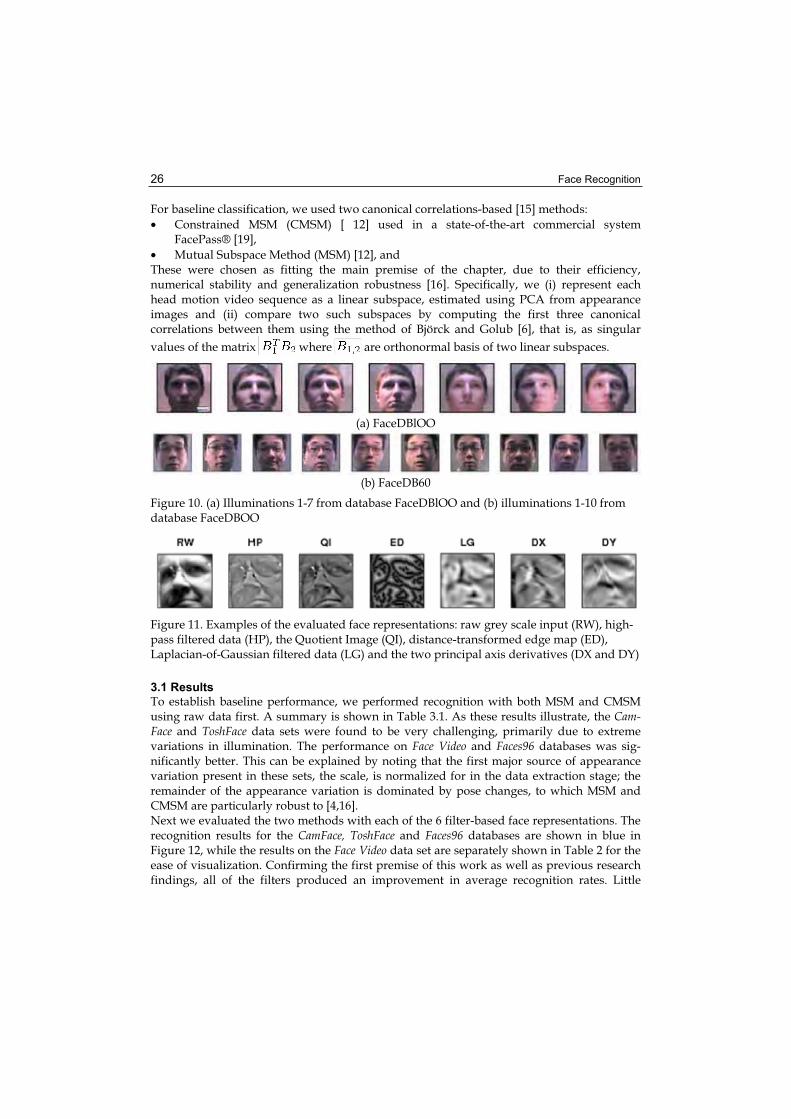
Methods and representations. The proposed framework was evaluated using the following filters (illustrated in Figure 11):
Face Recognition 26
For baseline classification, we used two canonical correlations-based [15] methods: • Constrained MSM (CMSM) [ 12] used in a state-of-the-art commercial system
FacePass® [19], • Mutual Subspace Method (MSM) [12], and These were chosen as fitting the main premise of the chapter, due to their efficiency, numerical stability and generalization robustness [16]. Specifically, we (i) represent each head motion video sequence as a linear subspace, estimated using PCA from appearance images and (ii) compare two such subspaces by computing the first three canonical correlations between them using the method of Björck and Golub [6], that is, as singular values of the matrix where are orthonormal basis of two linear subspaces.
(a) FaceDBlOO
(b) FaceDB60
Figure 10. (a) Illuminations 1-7 from database FaceDBlOO and (b) illuminations 1-10 from database FaceDBOO
Figure 11. Examples of the evaluated face representations: raw grey scale input (RW), high-pass filtered data (HP), the Quotient Image (QI), distance-transformed edge map (ED), Laplacian-of-Gaussian filtered data (LG) and the two principal axis derivatives (DX and DY)
3.1 Results
To establish baseline performance, we performed recognition with both MSM and CMSM using raw data first. A summary is shown in Table 3.1. As these results illustrate, the Cam-Face and ToshFace data sets were found to be very challenging, primarily due to extreme variations in illumination. The performance on Face Video and Faces96 databases was sig-nificantly better. This can be explained by noting that the first major source of appearance variation present in these sets, the scale, is normalized for in the data extraction stage; the remainder of the appearance variation is dominated by pose changes, to which MSM and CMSM are particularly robust to [4,16]. Next we evaluated the two methods with each of the 6 filter-based face representations. The recognition results for the CamFace, ToshFace and Faces96 databases are shown in blue in Figure 12, while the results on the Face Video data set are separately shown in Table 2 for the ease of visualization. Confirming the first premise of this work as well as previous research findings, all of the filters produced an improvement in average recognition rates. Little
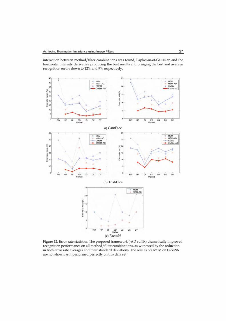
Achieving Illumination Invariance using Image Filters 27
interaction between method/filter combinations was found, Laplacian-of-Gaussian and the horizontal intensity derivative producing the best results and bringing the best and average recognition errors down to 12% and 9% respectively.
a) CamFace
(b) ToshFace
(c) Faces96
Figure 12. Error rate statistics. The proposed framework (-AD suffix) dramatically improved recognition performance on all method/filter combinations, as witnessed by the reduction in both error rate averages and their standard deviations. The results ofCMSM on Faces96 are not shown as it performed perfectly on this data set

Face Recognition 28
CamFace ToshFace FaceVideoDB Faces96 Average
CMSM 73.6 / 22.5 79.3 / 18.6 91.9 100.0 87.8
MSM 58.3 / 24.3 46.6 / 28.3 81.8 90.1 72.7
Table 1. Recognition rates (mean/STD, %)
RW HP Qi ED LG DX DY
MSM 0.00 0.00 0.00 0.00 9.09 0.00 0.00
MSM-AD 0.00 0.00 0.00 0.00 0.00 0.00 0.00
CMSM 0.00 9.09 0.00 0.00 0.00 0.00 0.00
CMSM-AD 0.00 0.00 0.00 0.00 0.00 0.00 0.00
Table 2. FaceVideoDB, mean error (%)
Finally, in the last set of experiments, we employed each of the 6 filters in the proposed data-adaptive framework. The recognition results are shown in red in Figure 12 and in Table 2 for the Face Video database. The proposed method produced a dramatic performance improvement in the case of all filters, reducing the average recognition error rate to only 3% in the case of CMSM/Laplacian-of-Gaussian combination.This is a very high recognition rate for such unconstrained conditions (see Figure 9), small amount of training data per gallery individual and the degree of illumination, pose and motion pattern variation between different sequences. An improvement in the robustness to illumination changes can also be seen in the significantly reduced standard deviation of the recognition, as shown in Figure 12. Finally, it should be emphasized that the demonstrated improvement is obtained with a negligible increase in the computational cost as all time-demanding learning is performed offline.
4. Conclusions
In this chapter we described a novel framework for automatic face recognition in the presence of varying illumination, primarily applicable to matching face sets or sequences. The framework is based on simple image processing filters that compete with unprocessed greyscale input to yield a single matching score between individuals. By performing all numerically consuming computation offline, our method both (i) retains the matching efficiency of simple image filters, but (ii) with a greatly increased robustness, as all online processing is performed in closed-form. Evaluated on a large, real-world data corpus, the proposed framework was shown to be successful in video-based recognition across a wide range of illumination, pose and face motion pattern changes.

Achieving Illumination Invariance using Image Filters 29
5. References
Y Adini, Y. Moses, and S. Ullman. Face recognition: The problem of compensating for changes in illumination direction. IEEE Transactions on Pattern Analysis and Machine Intelligence (PAMI), 19(7):721-732,1997. [1]
O. Arandjelovic and R. Cipolla. An illumination invariant face recognition system for access control using video. In Proc. IAPR British Machine Vision Conference (BMVC), pages537-546, September 2004. [2]
O. Arandjelovic and R. Cipolla. Face recognition from video using the generic shape-illumination manifold. In Proc. European Conference on Computer Vision (ECCV), 4:27-40, May 2006. [3]
O. Arandjelovic, G. Shakhnarovich, J. Fisher, R. Cipolla, and T. Darrell. Face recognition with image sets using manifold density divergence. In Proc. IEEE Conference on Computer Vision and Pattern Recognition (CVPR), 1:581-588, June 2005. [4]
O. Arandjelovic and A. Zisserman. Automatic face recognition for film character retrieval in feature-length films. In Proc. IEEE Conference on Computer Vision and Pattern Recognition (CVPR), 1:860-867, June 2005. [5]
A. Bjb'rck and G. H. Golub. Numerical methods for computing angles between linear subspaces. Mathematics of Computation, 27(123):579-594,1973. [6]
V. Blanz and T. Vetter. A morphable model for the synthesis of 3D faces. In Proc. Conference on Computer Graphics (SIGGRAPH), pages 187-194,1999. [7]
D. S. Bolme. Elastic bunch graph matching. Master's thesis, Colorado State University, 2003. [8]
J. Canny. A computational approach to edge detection. IEEE Transactions on Pattern Analysis and Machine Intelligence (PAMI), 8(6):679-698,1986. [9]
M. Everingham and A. Zisserman. Automated person identification in video. In Proc. IEEE International Conference on Image and Video Retrieval (CIVR), pages 289-298, 2004. [10]
A. Fitzgibbon and A. Zisserman. On affine invariant clustering and automatic cast listing in movies. In Proc. European Conference on Computer Vision (ECCV), pages 304-320, 2002. [11]
K. Fukui and O. Yamaguchi. Face recognition using multi-viewpoint patterns for robot vision. International Symposium of Robotics Research, 2003. [12]
Y. Gao and M. K. H. Leung. Face recognition using line edge map. IEEE Transactions on Pattern Analysis and Machine Intelligence (PAMI), 24(6):764-779, 2002. [13]
D. O. Gorodnichy. Associative neural networks as means for low-resolution video-based recognition. In Proc. International Joint Conference on Neural Networks, 2005. [14]
H. Hotelling. Relations between two sets of variates. Biometrika, 28:321-372,1936. [15] T-K. Kim, O. Arandjelovic, and R. Cipolla. Boosted manifold principal angles for image set-
based recognition. Pattern Recognition, 2006. (to appear). [16] S. Shan, W. Gao, B. Cao, and D. Zhao. Illumination normalization for robust face recognition
against varying lighting conditions. In Proc. IEEE International Workshop on Analysis and Modeling of Faces and Gestures, pages 157-164, 2003. [17]
B. Takacs. Comparing face images using the modified Hausdorff distance. Pattern Recognition, 31(12):1873-1881,1998. [18]
Toshiba. Facepass. www. toshiba. co. jp/mmlab/tech/w31e. htm. [19] P. Viola and M. Jones. Robust real-time face detection. International Journal of Computer Vision
(IJCV), 57(2): 137-154, 2004. [20]

Face Recognition 30
H. Wang, S. Z. Li, and Y. Wang. Face recognition under varying lighting conditions using self quotient image. In Proc. IEEE International Conference on Automatic Face and Gesture Recognition (FOR), pages 819-824, 2004. [21]
X. Wang and X. Tang. Unified subspace analysis for face recognition. In Proc. IEEE International Conference on Computer Vision (ICCV), 1:679-686, 2003. [22]
L. Wiskott, J-M. Fellous, N. Krtiger, and C. von der Malsburg. Face recognition by elastic bunch graph matching. Intelligent Biometric Techniques in Fingerprint and Face Recognition, pages 355-396,1999. [23]
3
Automatic Facial Feature Extraction for Face Recognition
Paola Campadelli, Raffaella Lanzarotti and Giuseppe Lipori Università degli Studi di Milano
Italy
1. Introduction
Facial feature extraction consists in localizing the most characteristic face components (eyes, nose, mouth, etc.) within images that depict human faces. This step is essential for the initialization of many face processing techniques like face tracking, facial expression recognition or face recognition. Among these, face recognition is a lively research area where it has been made a great effort in the last years to design and compare different techniques.In this chapter we intend to present an automatic method for facial feature extraction that we use for the initialization of our face recognition technique. In our notion, to extract the facial components equals to locate certain characteristic points, e.g. the center and the corners of the eyes, the nose tip, etc. Particular emphasis will be given to the localization of the most representative facial features, namely the eyes, and the locations of the other features will be derived from them. An important aspect of any localization algorithm is its precision. The face recognition techniques (FRTs) presented in literature only occasionally face the issue and rarely state the assumptions they make on their initialization; many simply skip the feature extraction step, and assume perfect localization by relying upon manual annotations of the facial feature positions.However, it has been demonstrated that face recognition heavily suffers from an imprecise localization of the face components. This is the reason why it is fundamental to achieve an automatic, robust and precise extraction of the desired features prior to any further processing. In this respect, we investigate the behavior of two FRTs when initialized on the real output of the extraction method.
2. General framework
A general statement of the automatic face recognition problem can be formulated as follows: given a stored database of face representations, one has to identify subjects represented in input probes. This definition can then be specialized to describe either the identification or the verification problem. The former requires as input a face image, and the system determines the subject identity on the basis of the database of known individuals; in the latter situation the system has to confirm or reject the identity claimed by the subject.

Face Recognition 32
As noted by [Zhao et al., 2003], whatever the problem formulation, its solution requires the accomplishment of three subsequent subtasks: face detection, feature extraction and facerecognition (Figure 1).
Figure 1. The subtasks of the face recognition problem
In fact, given an input image depicting one or more human subjects, the problem of evaluating their identity boils down to detecting their faces, extracting the relevant information needed for their description, and finally devising a matching algorithm to compare different descriptions. On one hand, the modularity of the original problem is a beneficial property as it allows to decompose it and to concentrate on the specific difficulties of each task in order to achieve a more effective solution. On the other hand, care must be taken in recomposing the separate modules: a common approach is to devise techniques that face only a task at once1 without considering the problems that can arise at the “interfaces” between them. In particular, most of face recognition techniques (FRTs) presented in literature skip the previous tasks and assume perfect feature extraction. While this can be certainly useful to develop and compare different recognition strategies, this attitude is not practical if the goal is to produce a fully automatic recognition system. Relying upon manual annotations of the feature positions does not account for the influence played by the extraction error on the recognition rate: the amount and trend of this dependency is not easily predictable and varies from FRT to FRT. These facts bring to two important observations: first of all it is fundamental to achieve an automatic, robust and precise extraction of the desired features prior to the application of a face recognition technique; secondly, it is important to study the relation between the quality of the feature extraction and the performance of the face recognition. By doing so, one ensures to couple only truly compatible modules to realize a fully automatic, robust system for face recognition. Differently stated, any FRT should be aware of the minimum precision required for its functioning and should clearly declare it. Regarding feature extraction, there is a general agreement that eyes are the most important facial features, thus a great research effort has been devoted to their detection and localization [Ji et al., 2005, Zhu and Ji, 2005, Fasel et al., 2005, Hamouz et al., 2005, Tang et al., 2005, Wang et al., 2005, Song et al., 2006, Gizatdinova and Surakka, 2006]. This is due to several reasons, among which: • eyes are a crucial source of information about the state of human beings.
1 Face detection and feature extraction are often accomplished simultaneously as it is possible to locate faces by directly locating their inner features.

Automatic Facial Feature Extraction for Face Recognition 33
• the eye appearance is less variant to certain typical face changes. For instance they are unaffected by the presence of facial hair (like beard or mustaches), and are little altered by small in-depth rotations and by transparent spectacles.
• the knowledge of the eye positions allows to roughly identify the face scale (the inter-ocular distance is relatively constant from subject to subject) and its in-plane rotation.
• the accurate eye localization permits to identify all the other facial features of interest.
To our knowledge, eyes are the only facial features required for the initialization of any FRT; actually this is the only information needed by those methods that operate an alignment of the face region, for instance as done by [Zhang et al., 2005]. However some techniques may require more features than just the eyes. For instance all FRTs derived from subspace methods (see [Shakhnarovich and Moghaddam, 2004] for a detailed survey) are initialized on four positions (the eyes, nose and mouth locations) to warp the face region before projection.2 Other techniques operate on larger sets of facial positions because they base the recognition on some kind of local processing: e.g. [Wiskott et al., 1999] is based on the comparison of the image texture found in the neighborhood of several fiducial points.Due to these considerations, the performance evaluation of a feature extraction method is usually given in terms of error measures that take into account only the localized eye positions. In Sec. 3. we will motivate the choice of such measures and we will introduce the study of the recognition rate in function of the eye localization precision. Sec. 4. presents the proposed algorithm for precise eye localization, together with the experimental results of its application on many public databases. In Sec. 5. we show a possible way to automatically derive the locations of a set of facial features from the knowledge of the sole eye positions. Sec. 6. reports the results of two face recognition experiments carried out on automatically extracted features: the behavior of two FRTs is discussed by making some considerations about their dependence on the extraction quality.
3. The importance of precise eye localization
Given the true positions of the eye centers (by manual annotation), the eye localization accuracy is expressed as a statistics of the error distribution made over each eye (usually the mean or the maximum), measured as the Euclidean pixel distance. In order to make these statistics meaningful, so that they can be used to compare the results obtained on any dataset, it is necessary to standardize the error by normalizing it over the face scale. One popular error measure has been introduced by [Jesorsky et al., 2001], and it has been already adopted by many research works on eye localization. The measure, which can be considered a worst case analysis, is defined as
2 Both the alignment and the warping are operations that intend to normalize a face database. The former consists in bringing the principal features (usually the eyes) to the same positions. This is done via an affine transformation (a scaling plus a roto-translation) that uses the eye centers as “pivots” of the transform. A warping is a non-affine transformation (a non uniform “stretching” of the face appearance) that is meant to densely align the face appearance (or at least the position of several features).

Face Recognition 34
where are the ground truth positions and the results of automatic localization. There is a general agreement [Jesorsky et al., 2001, Ma et al., 2004a, Zhou and Geng, 2004] that deye 0.25 is a good criterion to flag the eye presence (to claim eye detection). This precision roughly corresponds to a distance smaller than or equal to the eye width. However, this accuracy level may not be sufficient when the localized positions are used for the initialization of subsequent techniques.Following the idea presented in [Ma et al., 2004a], we studied the relation between deye and the face recognition rate of some baseline methods available in the CSU package [Beveridge et al., 2005] together with the LAIV-FRT described in Sec. 6. To mimic the behavior of eye localization techniques that achieve different levels of precision, we carried out four recognition experiments by artificially perturbing the ground truth quality; both Cr and Cl
have been randomly displaced inside circles of radii equal to 5%, 10% and 15% of Cl -Cr
with uniform distribution. In Figure 2 we report the results of this study on the XM2VTS database (see Appendix 8.). The experiment is defined as follows: session 1 is used for the gallery, session 2 for the probe, sessions 3 and 4 constitute the training set.3 Differently from [Ma et al., 2004a] where only the probe set is affected by artificial error, all three sets (gallery, probe and training) have been perturbed as it would happen in a completely automatic system. The graphs of Figure 2 clearly show that the precision of eye localization is critical for the alignment of faces, even if it does not affect all the methods in the same way.
Figure 2. Face recognition vs. (artificial) eye localization precision
Very recently in [Rodriguez et al., 2006] the issue has been further developed, suggesting a new error measure which is more discriminative than deye as it permits a quantitative evaluation of the face recognition degradation with respect to different error types. Instead of considering only the Euclidean distance between the detections and the ground truth points, it considers four kinds of error: the horizontal and the vertical error (both measured
3 The training set is needed by all the reported CSU methods, not by LAIV-FRT.
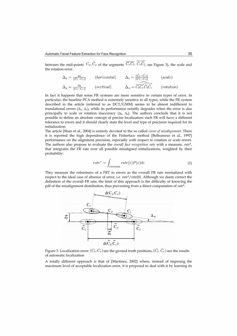
Automatic Facial Feature Extraction for Face Recognition 35
between the mid-points of the segments , see Figure 3), the scale and the rotation error.
In fact it happens that some FR systems are more sensitive to certain types of error. In particular, the baseline PCA method is extremely sensitive to all types, while the FR system described in the article (referred to as DCT/GMM) seems to be almost indifferent to translational errors ( x, y), while its performance notably degrades when the error is due principally to scale or rotation inaccuracy ( s, ). The authors conclude that it is not possible to define an absolute concept of precise localization: each FR will have a different tolerance to errors and it should clearly state the level and type of precision required for its initialization. The article [Shan et al., 2004] is entirely devoted to the so called curse of misalignment. There it is reported the high dependence of the Fisherface method [Belhumeur et al., 1997] performance on the alignment precision, especially with respect to rotation or scale errors. The authors also propose to evaluate the overall face recognition rate with a measure, rate*, that integrates the FR rate over all possible misaligned initializations, weighted by their probability:
(1)
They measure the robustness of a FRT to errors as the overall FR rate normalized with respect to the ideal case of absence of error, i.e. rate*/rate(0). Although we deem correct the definition of the overall FR rate, the limit of this approach is the difficulty of knowing the pdf of the misalignment distribution, thus preventing from a direct computation of rate*.
Figure 3. Localization error: are the ground truth positions, are the results of automatic localization
A totally different approach is that of [Martinez, 2002] where, instead of imposing the maximum level of acceptable localization error, it is proposed to deal with it by learning its
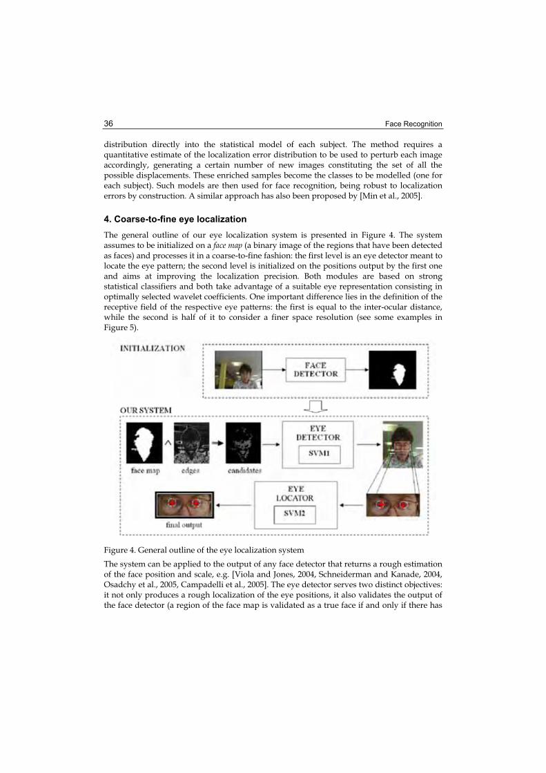
Face Recognition 36
distribution directly into the statistical model of each subject. The method requires a quantitative estimate of the localization error distribution to be used to perturb each image accordingly, generating a certain number of new images constituting the set of all the possible displacements. These enriched samples become the classes to be modelled (one for each subject). Such models are then used for face recognition, being robust to localization errors by construction. A similar approach has also been proposed by [Min et al., 2005].
4. Coarse-to-fine eye localization
The general outline of our eye localization system is presented in Figure 4. The system assumes to be initialized on a face map (a binary image of the regions that have been detected as faces) and processes it in a coarse-to-fine fashion: the first level is an eye detector meant to locate the eye pattern; the second level is initialized on the positions output by the first one and aims at improving the localization precision. Both modules are based on strong statistical classifiers and both take advantage of a suitable eye representation consisting in optimally selected wavelet coefficients. One important difference lies in the definition of the receptive field of the respective eye patterns: the first is equal to the inter-ocular distance, while the second is half of it to consider a finer space resolution (see some examples in Figure 5).
Figure 4. General outline of the eye localization system
The system can be applied to the output of any face detector that returns a rough estimation of the face position and scale, e.g. [Viola and Jones, 2004, Schneiderman and Kanade, 2004, Osadchy et al., 2005, Campadelli et al., 2005]. The eye detector serves two distinct objectives: it not only produces a rough localization of the eye positions, it also validates the output of the face detector (a region of the face map is validated as a true face if and only if there has

Automatic Facial Feature Extraction for Face Recognition 37
been at least an eye detection within it). In fact all face detectors manifest a certain false detection rate that must be dealt with.
Figure 5. Examples of eye patterns for the eye detector (first row) and locator (second row)
4.1 Wavelet selection
The difficulty intrinsic to the task of eye localization requires an accurate choice of a suitable representation of the eye pattern. It has been observed that the wavelet representation is more favorable than the direct representation as it leads to a smaller generalization error [Huang and Wechsler, 1999]. Haar-like wavelets permit to describe visual patterns in terms of luminance changes at different frequencies, at different positions and along different orientations.Before the wavelet decomposition, each eye patch undergoes an illumination normalization process (a contrast stretching operation) and is then reduced to 16×16 pixels.4 The decomposition is realized via an overcomplete bi-dimensional FWT (Fast Wavelet Transform) [Campadelli et al., 2006a] that produces almost four times as many coefficients with respect to the standard FWT. This redundancy is desirable as we want to increase the cardinality of the feature “vocabulary” before going through the selection procedure. In order to carry out the feature selection, we follow the idea proposed in [Oren et al., 1997] to apply a normalization step, which allows us to distinguish two sub-categories of wavelet coefficients: and . Both retain precious information: the first class gathers the coefficients that capture the edge structure of the pattern, while the second class contains the coefficients that indicate a systematic absence of edges (in a certain position, at a certain frequency and along a certain orientation). What is more important, the normalization step naturally defines a way to (separately) order the two categories, thus providing a way to assess the relative importance of the respective coefficients (for the technical details refer to [Campadelli et al., 2006b]). Once ordered the normalized coefficients, we define an error function to drive the selection process. We can measure the expressiveness of the coefficients by measuring how well they reconstruct the pattern they represent. We wish to find the set of optimal coefficients
(2)
4 Such a dimension represents a trade off between the necessity to maintain low the computational cost and to have sufficient details to learn the pattern appearance.

Face Recognition 38
where E is the mean eye pattern.5 U is the uniform pattern (with all pixels set to the mean luminance of E) and Ew is the reconstruction obtained by retaining the set w of the wavelet coefficients and . The first term of the objective function represents the error made by the reconstruction, while the second term intends to bound the amount of detail we are adding to the pattern representation (the value is a trade-off to balance between these two opposite goals). The ordering of the coefficients avoids to optimize over all the possible subsets of : w is incremented by iteratively adding new coefficients according to their ordering. We experimentally observed that the trend of the objective function is rather insensitive to variations of in the interval [0.5, 1]; we set it to 0.8. As it can be expected, the norm of the reconstruction maximally varies increasing the number of w+ retained, while it is almost unaffected by the number of selected w–. Due to this consideration, the selected
are such that they correspond to a local minimum of the objective function (2.), with the additional constraint .Figure 6 shows the coefficients selected for the pattern representation of each classifier. For the eye detector the process retains 95 wavelet coefficients that well characterize the general eye shape (the highest frequency coefficients are not considered). The representation associated with the eye locator keeps 334 coefficients, therefore the application of the second classifier is more costly than the first one.
Figure 6. From left to right: the mean eye pattern, its wavelet decomposition and the selected features (red contour) of the two eye patterns. High intensities correspond to strong edges, low intensities indicate uniform regions
4.2 Eye detection
The module for eye detection takes in a face map output by a generic face detector and produces a first, rough localization of the eye centers. Its core component is a strong statistical classifier that is capable of distinguishing the eye appearance from that of the other facial features; for this purpose we employ a binary Support Vector Machine (SVM), that is the state-of-the-art model for many classification tasks [Vapnik, 1995]. The classification is carried out on examples represented via a set of 95 selected wavelet filter responses, as described in the previous section. The training of the SVM has been carried out on a total of 13591 examples extracted from 1416 images: 600 belonging to the FERET database (controlled images of frontal faces), 416 to the BANCA database (to model different illumination conditions and the closed eyes), and 600 taken from a custom database containing many heterogenous and uncontrolled
5 Defined simply by averaging the gray levels of 2152 eye patterns.

Automatic Facial Feature Extraction for Face Recognition 39
pictures of various people (useful to model pose variations, non-neutral face expressions and random background examples). The positive class is built to contain eye examples cropped to a square of side equal to the inter-ocular distance. The negative class is populated by the other facial features (nose, mouth, chin, cheeks, forehead, etc.) and by some examples extracted from the background of images (respectively 3 and 2 for every positive). The definition of the two classes is driven by the notion that the eye detection module must be applied most of the time within the face region, therefore a negative example in this context is actually a facial feature distinct from the eyes. However, as face detectors sometimes detect some false positives, it is useful to enrich the definition of the negative class by adding random negative patterns. The machine is defined as follows: we employed a C-SVM (regulated by the error-penalization parameter C) based on the RBF kernel (parameterized by , which regulates the amplitude of the radial supports). The tuning of the two hyper-parameters Cand has been done in order to maximize the precision × recall6 on a test set of 6969 examples disjoint from the training set, but generated according to the same distribution. This procedure selected C = 6 and = 4.0 × 10⁻⁴, which yielded a SVM of 1698 support vectors (let us call it SVM1) and a 3.0% of misclassifications on the test set. This error can be considered an empirical estimate of the generalization error of the binary classifier. Once trained, the SVM1 is integrated into a pattern search strategy that avoids a multiscale scan: we infer the size of a hypothetical eye present in that region from the size of the face detector output.7 However, any face detector is subject to a certain error distribution on the size of its detections (either over-estimating or under-estimating the true face size), so the inferred eye scale cannot be fully trusted. We account for this uncertainty by considering a range of three scales; the evaluation of a candidate point P comes down to evaluating three examples centered in it: the one at the inferred scale (xP ), plus two examples (xP– and xP+ ) extracted in a way to account for an error distribution of the face size that is between half and twice the true size. This is a very reasonable requirement for a good face detector and permits to treat almost all of its outputs. If SVM1(x) = 0 is the equation of the decision function (hyperplane) separating the two classes, then we can treat the functional margin SVM1(x) as a “measure” of the confidence with which the SVM classifies the example x.Thus we define the function
as the strength of the candidate point P.Moreover, in order to make the search more efficient, we avoid an exhaustive scan of the candidate points: first comes the identification of points lying on edges, then they are subsampled with a step that depends on the scale of the face region;8 we consider as detections the points for which (P) > 0, and we group them according to their proximity in
6 If TP = true positives, FN = false negatives, FP = false positives
7 This relation has been estimated for each employed face detector and applied consistently. 8 The subsampling step is defined as , where the “radius” of a region is simply .

Face Recognition 40
the image;9 each group of point candidates is then represented by its centroid (the eye center) obtained weighting each point P with its (P). Ideally we should have just two eye centers detected for each face, however sometimes it happens that the eye classifier detects also one or more false positives. To deal with this, we introduce a selection criterion that exploits the margin of the classifier and assumes the substantial verticality of the face pose. Doing so, we manage to select the eye positions, and to discard the false detections, by choosing the couple of centers (ci, cj) that maximizes
where (ci)y is the y coordinate of the center ci. As we do not want to enforce the perfect verticality of the face, the square root at denominator is introduced to give more importance to the strength of the eye centers with respect to their horizontal alignment. Figure 7 visualizes the data flow of the eye detection module.
Figure 7. Eye detector outline
4.3 Eye localization
The module for eye localization is conceived to be applied in cascade to the eye detection one, when it is desirable a greater localization precision of the detected positions. The general architecture of this module is very similar to the previous one, therefore we can concentrate on the description of the main differences. While the eye detector must distinguish the global eye shape from that of other facial patterns, the eye locator must work at a much finer detail level: the goal here is to start from a rough localization and refine it by bringing it closer to the exact eye center location. Bearing in mind this objective, at this stage we consider a richer pattern representation (334 wavelet coefficients) that permits a finer spacing resolution. The positive examples
9 Two detections are “close”, and hence must be aggregated, if their Euclidean distance is smaller than five times the subsampling step. This multiple is not arbitrary, as it corresponds to about half the distance between the eye corners.

Automatic Facial Feature Extraction for Face Recognition 41
correspond to a smaller receptive field (half of the inter-ocular distance) and the negative examples are generated by small, random displacements of the subimages used for the extraction of the positive ones (10 negative examples for each positive). The C-SVM with RBF kernel is first tuned in the same way as before, selecting C = 1.35 and
= 3.6 × 10⁻⁴. The training is then carried on over 22647 examples, producing a SVM of 3209 support vectors (SVM2 from now on) that exhibits a misclassification rate of 2.5% on a test set of 11487 examples. The output of the eye detection module is used for the initialization of the eye localization module. The pattern search proceeds only in a small neighborhood of the starting locations, but this time we do an exhaustive scan as we do not want to loose spacial resolution. The search is done at only one scale, inferred averaging the three scales previously considered and weighting them according to their respective SVM1 margin (the factor is due to the smaller receptive field):
where
Finally the SVM2 evaluations are thresholded at 0, determining a binary map consisting of one or more connected regions. The refined eye center is found at the centroid of the connected region that weights the most according to the SVM2 margin. Figure 8 visualizes the data flow of the eye localization module.
Figure 8. Eye locator outline
We note here that the computational cost of each single SVM evaluation is linearly proportional to the number of support vectors. Therefore, in order to reduce the computational time of our application, it would be desirable to approximate the hyperplane associated to the SVM by reducing the number of its supports, without deteriorating its separation abilities. Some research has been devoted to optimal approximation techniques for support vector reduction, which usually require to specify aforetime the desired number of supports to retain at the end of the reduction process [Burges, 1996, Schölkopf et al., 1999]. However there is no general rule regarding how many vectors can be suppressed before compromising the performance of a SVM classifier; this quantity clearly depends on the difficulty of the classification task. Another approach consists in fixing a threshold on the maximum marginal difference of the old support vectors with respect to the new hyperplane [Nguyen and Ho, 2005]. This perspective is particularly interesting as it enables

Face Recognition 42
to specify a stop quantity that is no more arbitrary, on the contrary it allows to limit the oscillation of the decision surface.We have reimplemented the technique described in [Nguyen and Ho, 2005] and applied it only to the SVM2 because a reduction of this machine would be of great benefit with regards to the computational time: in fact it is composed of almost twice as many support vectors than the SVM1, and it is evaluated at many more candidate points. What is more, while a reduction of the SVM1 strongly influences the eye detection rate, a reduced SVM2 only degrades the localization precision, and in a much more progressive way. The results of the reduction experiments are given in the next section.
4.4 Eye localization results
The experiments have been carried out on images taken from the following datasets: XM2VTS, BANCA, FRGC v.1.0, BioID and FERET (see Appendix 8. for the full specification of the datasets composition). All these images depict one subject shot with vertical, frontal pose, eyes closed or open, presence or absence of spectacles; none of these images has been used for the training of the SVM classifiers. On color images (XM2VTS, BANCA, FRGC) the face detection has been carried out using the method in [Campadelli et al., 2005], while when the input images are gray scale (BioID, FERET), the detection is performed by a re-implementation of [Viola and Jones, 2001].
Figure 9. The cumulative distributions of eye detection and localization over different databases
The graphs in Figure 9 display the performance of the eye detector (SVM1), the eye locator (SVM2) and, when available, we report the performance achieved by the methods presented by [Hamouz et al., 2005] (denoted as “1 face on the output” in the original article) and [Cristinacce and Cootes, 2006] (Constrained Local Models, CLM). Regarding CLM, the curves plotted on the BioID and XM2VTS graphs have been extrapolated from the results kindly provided by the authors of the method.

Automatic Facial Feature Extraction for Face Recognition 43
The numbers reported in parenthesis on the graphs represent the Area Under the Curve (AUC), therefore they give a global estimation of the performance of each localization method over that particular dataset. Regarding eye detection, the SVM1 alone permits to achieve rates of 99.0%, 95.5%, 95.6%, 97.1% and 97.8% over the datasets BANCA, BioID, FERET, FRGC and XM2VTS respectively (deye 0.25). As expected, the addition of the second classifier greatly improves the precision of the detection and the curves are systematically above the rates declared by Hamouz et al. Regarding CLM, we note that it is very effective in localizing the eyes over the BioID database, while on the XM2VTS it achieves a lower rate.10
Also the works by [Jesorsky et al., 2001], [Ma et al., 2004b], [Tang et al., 2005] and [Niu et al., 2006] use the error measure deye in order to assess the quality of eye localization. The first work exhibits a localization performance that is lower than that reported by Hamouz et al. The second one presents a cumulative curve that looks similar to the performance of the SVM1 but it is obtained referring to a mix of databases with no intersection with the ones we considered, making impossible a direct comparison. The third paper reports results on the BioID, tabulating only the values corresponding to deye 0.1 and deye 0.25 (91.8% and 98.1% respectively), while omitting the curve behavior under this value. Finally, the last work presents results on XM2VTS and BioID; we do not report them in figure since the values are not clearly tabulated, however we note that the performance on XM2VTS is comparable to ours, while on the BioID their results are significantly better. Other works face the same problem, while adopting a different metrics. For instance [Wang et al., 2005] adopt a normalized mean error (not the maximum) and give an error of 2.67% on the entire FRGC. By adopting this measure on the considered FRGC subsets we observe an error of 3.21%. Analogously, [Fasel et al., 2005] provide the localization results on the BioID in terms of the mean relative error, this time expressed in iris units. Noting that the iris diameter is slightly shorter than the 20% of the inter-ocular distance, their measurement corresponds to a mean error (relative to the inter-ocular distance) of 0.04, while we report a mean relative error of 0.031. The method described by [Everingham and Zisserman, 2006] carries out the experiments on the FERET database: in the 90% of images the mean relative error is reported to be smaller or equal to 0.047, which is remarkable (for the same level of precision, on the FERET we count about the 81% of images). We also present in Figure 10 the histograms of x, y, s, (recall Sec. 3.) made by our eye localization module on all the datasets previously considered; for comparison, we report in Figure 11 the results of the CLM algorithm on the available datasets (BioID, XM2VTS). Referring to the FR algorithm DCT/GMM proposed by [Rodriguez et al., 2006], we observe that each error histogram generated by the coarse-to-fine technique is entirely included within the declared error tolerance (rotation error [-10°, 10°], translational error [-0.2, 0.2], scale error [0.8, 1.2]). In the spirit of their article, we conclude that our application would be appropriate for the initialization of DCT/GMM.
The speed was not the main focus of our research, giving that nowadays there exist dedicated architectures which would allow to obtain a real-time application. Running java interpreted code on a Pentium 4 with 3.2GHz, we report the computational time of the two
10 The authors attribute this behavior to the major similarity of BioID images to the images used to train CLM.
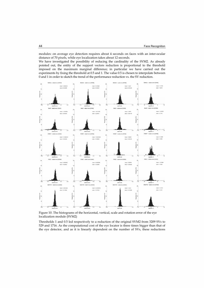
Face Recognition 44
modules: on average eye detection requires about 4 seconds on faces with an inter-ocular distance of 70 pixels, while eye localization takes about 12 seconds. We have investigated the possibility of reducing the cardinality of the SVM2. As already pointed out, the entity of the support vectors reduction is proportional to the threshold imposed on the maximum marginal difference; in particular we have carried out the experiments by fixing the threshold at 0.5 and 1. The value 0.5 is chosen to interpolate between 0 and 1 in order to sketch the trend of the performance reduction vs. the SV reduction.
Figure 10. The histograms of the horizontal, vertical, scale and rotation error of the eye localization module (SVM2)
Thresholds 1 and 0.5 led respectively to a reduction of the original SVM2 from 3209 SVs to 529 and 1716. As the computational cost of the eye locator is three times bigger than that of the eye detector, and as it is linearly dependent on the number of SVs, these reductions
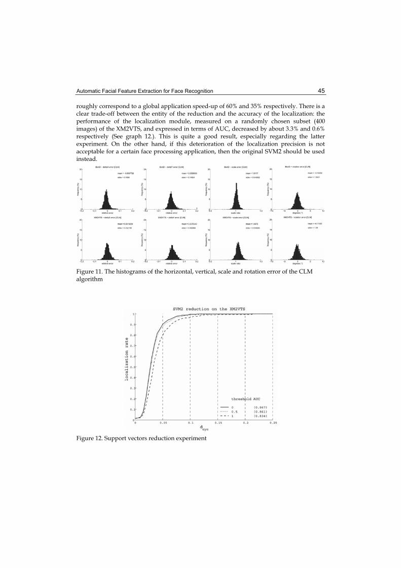
Automatic Facial Feature Extraction for Face Recognition 45
roughly correspond to a global application speed-up of 60% and 35% respectively. There is a clear trade-off between the entity of the reduction and the accuracy of the localization: the performance of the localization module, measured on a randomly chosen subset (400 images) of the XM2VTS, and expressed in terms of AUC, decreased by about 3.3% and 0.6% respectively (See graph 12.). This is quite a good result, especially regarding the latter experiment. On the other hand, if this deterioration of the localization precision is not acceptable for a certain face processing application, then the original SVM2 should be used instead.
Figure 11. The histograms of the horizontal, vertical, scale and rotation error of the CLM algorithm
Figure 12. Support vectors reduction experiment

Face Recognition 46
5. From eye centers to fiducial points
In this section we show how, given the eye centers, we derive a set of 27 characteristic points (fiducial points): three points on each eyebrow, the tip, the lateral extremes and the vertical mid-point of the nose, the eye and lip corners, their upper and lower mid-points, the mid-point between the two eyes, and four points on the cheeks (see Figure 13). This module has been conceived to work on still color images of good quality, acquired with uniform illumination, where the face is almost frontal and the subject assumes either a neutral or a slightly smiling expression. The method proceeds in a top-down fashion: given the eye centers, it derives the eye, nose and mouth subimages on the basis of simple geometrical considerations, and extracts the corresponding fiducial points (green points in Figure 13) as described in the following. Finally, in order to enrich the face description, further fiducial points (red points in Figure 13) are inferred on the basis of the position of the extracted points.
Figure 13. A face is described by 27 fiducial points: 13 are directly extracted from the image (in green), 14 are inferred from the former ones (in red)
5.1 Eyes
The eyes are described by a parametric model which is a simplified version (6 parameters instead of 11) of the deformable template proposed in [Yuille et al., 1992]. The eye model is made of two parabolas, representing the upper and lower eye arcs, and intersecting at the eye corners (see Figure 14); the model parameters, ,are: the model eye center coordinates (xt, yt), the eye upper and lower half-heights a and c,

Automatic Facial Feature Extraction for Face Recognition 47
the eye half-width b, and the rotation angle t expressing the rotation of the model with respect to the horizontal axis. The fundamental step to obtain good results is a very precise initialization of the template parameters. To this end, the eye center coordinates, (xc, yc), derived by the SVM2, are used as initial values for (xt, yt). In order to find a good initial estimate for the parameters a, b, c, we carried out a statistical study on 2000 images to evaluate the relation between the inter-ocular distance d and both the semi-width, b and the semi-height of the eye, a and c,obtaining very stable results: the mean values are 5.6 and 12 respectively, with small variance values (0.8 and 1.2), making these evaluations reliable and useful to set the initial values of the parameters a, b, c correspondingly. The last parameter, , is set initially to the estimated face tilt.
Figure 14. Deformable eye template
In order to adapt the generic template to a specific eye, we minimize an energy function Et
that depends on the template parameters (prior information on the eye shape) and on certain image characteristics (edges and the eye sclera). The characteristics are evaluated on the u plane of the CIE-Luv11 space, since in this color plane the information we are looking for (edges and eye sclera) are strengthened and clearer (see Figure 15 b,c). More precisely:
where:
1.2. ,
being Rw the upper and lower parabolas, and e the edge image obtained applying the Sobel filter to the eye subimage.
3. ,where Rw is the region enclosed between the two parabolas, and i is a weighted image called eye map, and determined as follows: • threshold the u plane with a global threshold:
th = 0.9 × max(u)
11 Uniform color space introduced by the CIE (Commission Internationale de l’Eclairage) to properly represent distances between colors [Wyszecki and Stiles, 1982].

Face Recognition 48
• adapt the threshold until the pixels set to 1 are symmetrically distributed around the eye center.
• for every pixel p
The function is optimized adopting a search strategy based on the steepest descent, as suggested in Yuille’s work; once obtained the eye contour description, we derive the two eye corners and the upper and lower mid-points straightforwardly (see Figure 15).
5.2 Nose
The nose is characterized by very simple and generic properties: the nose has a “base” the gray levels of which contrast significantly with the neighboring regions; moreover, the nose profile can be characterized as the set of points with the highest symmetry and high luminance values; therefore we can identify the nose tip as the point that lies on the nose profile, above the nose baseline, and that corresponds to the brightest gray level. These considerations allow to localize the nose tip robustly (see Figure 16).
Figure 15. Eye points search: a) eye subimage b) edge image c) eye map d) initial template position e) final template position f ) fiducial points
Figure 16. Examples of nose processing. The black horizontal line indicates the nose base; the black dots along the nose are the points of maximal symmetry along each row; the red line is the vertical axis approximating those points; the green marker indicates the nose tip
5.3 Mouth
Regarding the mouth, our goal is to locate its corners and its upper and lower mid-points. To this aim, we use a snake [Hamarneh, 2000] to determine the entire contour since we verified that they can robustly describe the very different shapes that mouths can assume. To make the snake converge, its initialization is fundamental; therefore the algorithm estimates the mouth corners and anchors the snake to them: first, we represent the mouth subimage in the YCbCr color space, and we apply the following transformation:
MM = (255 - (Cr - Cb)) Cr 2
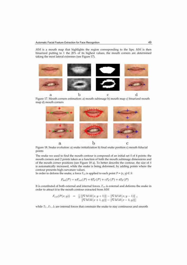
Automatic Facial Feature Extraction for Face Recognition 49
MM is a mouth map that highlights the region corresponding to the lips; MM is then binarized putting to 1 the 20% of its highest values; the mouth corners are determined taking the most lateral extremes (see Figure 17).
Figure 17. Mouth corners estimation: a) mouth subimage b) mouth map c) binarized mouth map d) mouth corners
Figure 18. Snake evolution: a) snake initialization b) final snake position c) mouth fiducial points
The snake we used to find the mouth contour is composed of an initial set S of 4 points: the mouth corners and 2 points taken as a function of both the mouth subimage dimensions and of the mouth corner positions (see Figure 18 a). To better describe the contour, the size of Sis automatically increased, while the snake is being deformed, by adding points where the contour presents high curvature values. In order to deform the snake, a force Ftot is applied to each point P = (x, y) S:
It is constituted of both external and internal forces. Fext is external and deforms the snake in order to attract it to the mouth contour extracted from MM
while TF , FF , IF are internal forces that constrain the snake to stay continuous and smooth

Face Recognition 50
where is the vector in P(x, y) normal to the snake. The algorithm adds points and deforms the snake until the global force Ftot is lower than a certain tolerance for a fixed number of consequent steps. Once obtained the mouth contour description, we derive the fiducial points straightforwardly. Figure 18 reports some results; we notice that the described method achieves good results both on closed and open mouths.
5.4 Evaluation of the fiducial points precision
In order to quantitatively evaluate the precision of the extracted fiducial points (FP), we adopt the error measure dFP that can be considered an extension of deye to a bigger set of features
where is the localized position of a fiducial point and P is the corresponding ground truth. Notice that dFP is a statistics different from deye as it averages the localization errors instead of taking their maximum. On one hand this is a less demanding criterion, however it is a more representative measure of a larger set of features. Unfortunately, such performance evaluation is rarely given in the related literature. As we have been provided with the localization output of the CLM method on the XM2VTS database, we are able to compare it with our own. On the 9 fiducial points that are common to both methods (eye corners, nose tip, mouth corners and mid-points), we obtain a dFP
equal to 0.051 while CLM achieves 0.056. Regarding solely our method, if we take into account also the 4 eye mid-points, the precision considerably improves to 0.045. The remaining 14 fiducial points are not considered for the performance evaluation because they are inferred from the other 13 and their precision is correlated. Furthermore, a disjoint analysis of the precision achieved over each fiducial point highlights that the nose tip is the most critical one (mean error of 0.07), while the points lying around the eyes are the most precisely determined (mean error of 0.03).
6. Face recognition experiment
We set up a simple face recognition experiment to investigate the behavior of two different FRTs when initialized on real outputs of our feature extraction method. The techniques, LAIV and CAS, have been chosen in such a way to represent two different processing paradigms: the former is based on local features, the latter treats the information at the global face level. For this experiment we do not consider any more the CSU baseline methods considered in Sec. 3. since they are not state-of-the-art FRTs, being their purpose only comparative. Instead, LAIV and CAS are very recent methods which are reported to score high recognition rates.

Automatic Facial Feature Extraction for Face Recognition 51
The experiment has two aims: to compare the absolute performance achieved by either method; to analyze the relative performance decay of each FRT in function of the eye localization precision.
LAIV-FRT: This technique is a feature-based FRT described in [Arca et al., 2006]. Given the eye positions, it uses the technique described in Sec. 5. to automatically locate the position of 27 fiducial points. Each fiducial point is characterized by extracting square patches centered in them and convolving those with the Gabor filter bank described in [Wiskott et al., 1999]. The resulting 40 coefficients are complex numbers, and the jet J is obtained by considering only the magnitude part. Thus, the face characterization consists of a jets vector of 40 × 27 real coefficients. The recognition task becomes the problem of finding a suitable similarity measure between jets. The LAIV technique introduces the idea of considering only the set of points for which the corresponding jets have high similarity. In particular, to recognize a test image t, it is compared one-to-one with each image i belonging to the gallery G, producing a similarity score, and it is recognized as the subject i* which obtained the highest score: • for each image i G and each fiducial point k = 0, .., 26, compute the similarity measure
between pairs of corresponding Jets:
where z = 0, ..., 39 and Jt,k is the Jet in the test image corresponding to the kth fiducial point.
• for each fiducial point k, order the values {Si,k} in descending order, and assign to each of them a weight wi,k as a function of its ordered position pi,k:
where , and c is a normalization factor. • for each gallery image i, the similarity score is obtained as a weighted average of the
pairwise jet similarity, limited to the set BestPoints of + 1 = 14 points with highest weight:
This technique gives better results than considering the average of all similarities, since it allows to discard wrong matches on single points: if some fiducial points are not precisely localized either in the test or in the gallery image, they will have low similarity measures and will not belong to the set BestPoints, so they will not be used for recognition. CAS-FRT: We consider here a custom reimplementation of the method proposed by [Zhang et al., 2005]; the authors have successively developed the technique in [Shan et al., 2006], which however requires an extremely long learning phase.
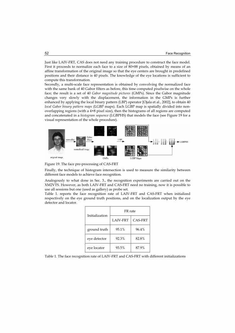
Face Recognition 52
Just like LAIV-FRT, CAS does not need any training procedure to construct the face model. First it proceeds to normalize each face to a size of 80×88 pixels, obtained by means of an affine transformation of the original image so that the eye centers are brought in predefined positions and their distance is 40 pixels. The knowledge of the eye locations is sufficient to compute this transformation. Secondly, a multi-scale face representation is obtained by convolving the normalized face with the same bank of 40 Gabor filters as before, this time computed pixelwise on the whole face; the result is a set of 40 Gabor magnitude pictures (GMPs). Since the Gabor magnitude changes very slowly with the displacement, the information in the GMPs is further enhanced by applying the local binary pattern (LBP) operator [Ojala et al., 2002], to obtain 40 local Gabor binary pattern maps (LGBP maps). Each LGBP map is spatially divided into non-overlapping regions (with a 4×8 pixel size), then the histograms of all regions are computed and concatenated in a histogram sequence (LGBPHS) that models the face (see Figure 19 for a visual representation of the whole procedure).
Figure 19. The face pre-processing of CAS-FRT
Finally, the technique of histogram intersection is used to measure the similarity between different face models to achieve face recognition.
Analogously to what done in Sec. 3., the recognition experiments are carried out on the XM2VTS. However, as both LAIV-FRT and CAS-FRT need no training, now it is possible to use all sessions but one (used as gallery) as probe set. Table 1. reports the face recognition rate of LAIV-FRT and CAS-FRT when initialized respectively on the eye ground truth positions, and on the localization output by the eye detector and locator.
FR rate Initialization
LAIV-FRT CAS-FRT
ground truth 95.1% 96.4%
eye detector 92.3% 82.8%
eye locator 93.5% 87.9%
Table 1. The face recognition rate of LAIV-FRT and CAS-FRT with different initializations

Automatic Facial Feature Extraction for Face Recognition 53
It can be noted that CAS-FRT performs better than LAIV-FRT (96.4% vs. 95.1%) when it is manually and precisely initialized, but its performance drops dramatically when an automatic eye localization method is used. On the contrary, LAIV-FRT proves to be more robust with respect to localization errors; indeed, it can overcome slight mis-initializations. It can be stated that LAIV-FRT behaves globally better than CAS-FRT as it is more robust in the spirit of Eq. (1). This difference in performance is probably due to the global nature of CAS initialization: if the eye centers estimation is mistaken, the error will propagate to the rest of the face regions due to the global affine transformation. Also in the case of LAIV-FRT the error affects the computation, but in a more local sense: first of all, this FRT relies on the measured inter-ocular distance to scale the Gabor filters, however the histogram of the scale error is quite narrow (see the third graph of the last row of Figure 10); secondly, a slightly wrong initialization of the employed templates is often recovered by the template matching algorithms. Anyways, even when a full recovery is not attained, the selection criterion of the BestPoints set allows to discard the unreliable fiducial points and LAIV-FRT still manages to recognize the face in a number of cases. On the other hand, it should be observed that the presence of the intermediate module described in Sec. 5., and the discard operated by the selection criterion, weaken the dependency between the eye localization precision and the recognition rate, so that the performance results on the different initializations are very similar. The same phenomenon explains the results of the experiment reported in Figure 2 regarding artificially perturbed manual annotations: all the considered CSU face recognition techniques start from a global representation of the face and hence are greatly affected by misalignments.
7. Conclusion
The subject of this chapter is the presentation of a novel method for the automatic and precise localization of facial features in 2D still images. The method follows the top-down paradigm and consists of subsequent steps to decompose the initial problem in increasingly easier tasks: assuming a rough localization of the face in the image, first comes the application of an eye detector with the aim of discriminating between real face regions and possible false positives. The accuracy of the detection is nearly optimal. Successively, an eye locator is applied on a small neighborhood of the detector output to improve the localization precision. Finally, the eye center positions are used to derive 27 facial fiducial points, either extracted directly from the image or inferred on the basis of simple geometrical considerations. The eye localization module has been extensively tested on five publicly available databases with different characteristics to remark its generality. In the overall, the results are comparable to or better than those obtained by the state-of-the-art methods. The performance evaluation is carried out according to two objective performance measures in order to favor the comparison with other techniques. Concerning the fiducial point localization, results on the XM2VTS show high precision. In the last years many research works have pointed out the importance of facial feature localization as the fundamental step for the initialization of other methods, mostly face recognition techniques. In general, not all types of error affect the subsequent processing in the same way: for instance scale errors usually affect a FR technique more than translational

Face Recognition 54
misalignment. Moreover, face recognition techniques manifest a different tolerance to the localization error depending on the nature of their initialization. We conducted some experiments which suggest that, as the localization precision decreases, the recognition rate decays more rapidly for those methods which start from a global face representation. However, since different FR techniques exhibit a different robustness to certain types and amount of error, there exists no absolute threshold for precise localization. The authors of face recognition techniques should investigate the robustness of their methods with respect to misalignments, in order to state the error tolerance that they assume when declaring the face recognition rate. Both the obtained localization results and the survey of recent eye localization techniques clearly show that we are far from perfect localization and there is still room for improvement.
8. Appendix: datasets
This appendix details the definition of the considered public databases, specifying for each of them which images have been used to carry out the experimental tests. In alphabetical order:• The [BANCA DB, web] of English people consists of three sections referred to as
Controlled, Adverse and Degraded. The latter is not considered as the images are particularly blurred, making the step of precise eye localization useless. Regarding the former:• Controlled: it consists of 2080 images each one representing one person placed in
front of the camera and standing on a uniform background. The database collects pictures of 52 people of different ethnic groups (Caucasian, Indians, Japanese, Africans, South-Americans), acquired in 4 different sessions (10 images per subject in each session). The illumination conditions vary from daylight to underexposed, while no evident chromatic alteration is present.
• Adverse: like the Controlled section it consists of 2080 images, each one representing one person placed in front of the camera and looking down as if reading, while in this section the background is non-uniform. The image quality and illumination are not very good.
The selected test set is composed of the first image of each subject in each section, for a total of 416 images.
• The [BioID DB, web] is formed of 1521 gray scale images of close-up faces. The number of images per subject is variable, as it is the background (usually cluttered like in an office environment). The tests reported in the previous sections refer to the whole database.
• The [FERET DB, web] database consists of 10 gray level images per person organized according to the out of plane rotation: 0°, ±15°, ±25°, ±40° or ±60°; regarding the sole frontal views the set contains two images per subject, one smiling, one with neutral expression.The considered test set consists of 1000 images randomly selected from the images with rotation up to ±15°.

Automatic Facial Feature Extraction for Face Recognition 55
• The [FRGC DB, web] database version 1.0 collects 5658 high resolution images of 275 subjects in frontal position, arranged in two sections: controlled and uncontrolled. The images are organized in subject sessions: each contains 4 images acquired in controlled conditions (uniform background and homogeneous illumination) and 2 in uncontrolled conditions (generic background and varying illumination conditions). In both conditions, half of the images represent the subject while smiling, the remaining half with neutral expression. The number of sessions varies from subject to subject, between 1 and 7. The considered test set is composed of both 473 controlled and 396 uncontrolled images. These numbers are obtained by taking, for each subject, the first controlled image of the first two sessions (when the second is present).
• The [XM2VTS DB, web] consists of 1180 high quality images of single faces acquired in frontal position and with homogeneous background; some of the subjects wear spectacles. The pictures are grouped into 4 sessions of 295 subjects each. The conducted tests refer to the whole database.
9. References
Arca, S., Campadelli, P., and Lanzarotti, R. (2006). A face recognition system based on automatically determined facial fiducial points. Pattern Recognition, 39(3):432–443. [Arca et al., 2006]
BANCA DB (web). Address: http://www.ee.surrey.ac.uk/Research/VSSP/banca/.[BANCA DB, web]
Belhumeur, P., Hespanha, J., and Kriegman, D. (1997). Eigenfaces vs. Fisherfaces: Recognition using class specific linear projection. IEEE Trans. Pattern Analysis and Machine Intelligence, 19(7):711–720. [Belhumeur et al., 1997]
Beveridge, J., Bolme, D., Draper, B., and Teixeira, M. (2005). The CSU face identification evaluation system. its purpose, features, and structure. Machine vision and applications, 16:128–138. [Beveridge et al., 2005]
BioID DB (web). Address: http://www.humanscan.de/support/downloads/facedb.php. [BioID DB, web]
Burges, C. (1996). Simplified Support Vector decision rules. Int’l Conf. Machine Learning,pages 71–77. [Burges, 1996]
Campadelli, P., Lanzarotti, R., and Lipori, G. (2005). Face localization in color images with complex background. Proc. IEEE Int’l Workshop on Computer Architecture for Machine Perception, pages 243–248. [Campadelli et al., 2005]
Campadelli, P., Lanzarotti, R., and Lipori, G. (2006a). Eye localization and face recognition. RAIRO - Theoretical Informatics and Applications, 40:123–139. [Campadelli et al., 2006a]
Campadelli, P., Lanzarotti, R., and Lipori, G. (2006b). Precise eye localization through a general-to-specific model definition. Proceedings of the British Machine Vision Conference, 1:187–196. [Campadelli et al., 2006b]
Cristinacce, D. and Cootes, T. (2006). Feature detection and tracking with constrained local models. Proc. the British Machine Vision Conf., 3:929–938. [Cristinacce and Cootes, 2006]

Face Recognition 56
Everingham, M. and Zisserman, A. (2006). Regression and classification approaches to eye localization in face images. Proceedings of the 7th International Conference on Automatic Face and Gesture Recognition (FG2006), pages 441–446. [Everingham and Zisserman, 2006]
Fasel, I., Fortenberry, B., and Movellan, J. (2005). A generative framework for real time object detection and classification. Computer Vision and Image Understanding, 98:182–210. [Fasel et al., 2005]
FERET DB (web). Address: http://www.itl.nist.gov/iad/humanid/feret/.[FERET DB, web] FRGC DB (web). Address: http://www.frvt.org/FRGC/.[FRGC DB, web] Gizatdinova, Y. and Surakka, V. (2006). Feature-based detection of facial landmarks from
neutral and expressive facial images. IEEE Trans. Pattern Analysis and Machine Intelligence, 28(1):135–139. [Gizatdinova and Surakka, 2006]
Hamarneh, G. (2000). Image segmentation with constrained snakes. Swedish Image Analysis Society Newsletter SSABlaskan, 8:5–6. [Hamarneh, 2000]
Hamouz, M., Kittler, J., Kamarainen, J., Paalanen, P., Kälviäinen, H., and Matas, J. (2005). Feature-based affine invariant localization of faces. IEEE Trans. Pattern Analysis and Machine Intelligence, 27(9):1490–1495. [Hamouz et al., 2005]
Huang, J. and Wechsler, H. (1999). Eye detection using optimal wavelet packets and radial basis functions (RBFs). Int’l Journal of Pattern Recognition and Artificial Intelligence,13(7):1009–1026. [Huang and Wechsler, 1999]
Jesorsky, O., Kirchberg, K., and Frischholz, R. (2001). Robust face detection using the Hausdorff distance. Lecture Notes in Computer Science, 2091:212 – 227. [Jesorsky et al., 2001]
Ji, Q., Wechsler, H., Duchowski, A., and Flickner, M. (2005). Special issue: eye detection and tracking. Computer Vision and Image Understanding, 98(1):1–3. [Ji et al., 2005]
Ma, Y., Ding, X., Wang, Z., and Wang, N. (2004a). Robust precise eye location under probabilistic framework. Proc. IEEE Int’l Conf. Automatic Face and Gesture Recognition, pages 339–344. [Ma et al., 2004a]
Ma, Y., Ding, X., Wang, Z., and Wang, N. (2004b). Robust precise eye location under probabilistic framework. Proc. IEEE Int’l Conf. Automatic Face and Gesture Recognition. [Ma et al., 2004b]
Martinez, A. (2002). Recognizing imprecisely localized, partially occluded, and expression variant faces from a single sample per class. IEEE Trans. Pattern Analysis and Machine Intelligence, 24(6):748–763. [Martinez, 2002]
Min, J., Bowyer, K. W., and Flynn, P. J. (2005). Eye perturbation approach for robust recognition of inaccurately aligned faces. Proc. of the Internationl Conf. Audio and Video based Biometric Person Authentication (AVBPA), LCNS 3546:41–50. [Min et al., 2005]
Nguyen, D. and Ho, T. (2005). An efficient method for simplifying Support Vector Machines. Proc. Int’l Conf. Machine learning, pages 617–624. [Nguyen and Ho, 2005]
Niu, Z., Shan, S., Yan, S., Chen, X., and Gao, W. (2006). 2D Cascaded AdaBoost for Eye Localization. Proc. of the 18th Internationl Conference on Pattern Recognition, 2:1216–1219. [Niu et al., 2006]
Ojala, T., Pietikäinen, M., and Mäenpää, T. (2002). Multiresolution grayscale and rotation invariant texture classification with local binary patterns. IEEE Transactions on Pattern Analysis and Machine Intelligence, 24(7):971–987. [Ojala et al., 2002]

Automatic Facial Feature Extraction for Face Recognition 57
Oren, M., Papageorgiou, C., Sinha, P., Osuna, E., and Poggio, T. (1997). Pedestrian detection using wavelet templates. In Proc. Computer Vision and Pattern Recognition, pages 193–199. [Oren et al., 1997]
Osadchy, M., Miller, M., and LeCun, Y. (2005). Synergistic face detection and pose estimation with energy-based models. In Saul, L. K., Weiss, Y., and Bottou, L., editors, Advances in Neural Information Processing Systems, volume 17, pages 1017–1024. MIT Press. [Osadchy et al., 2005]
Rodriguez, Y., Cardinaux, F., Bengio, S., and Mariéthoz, J. (2006). Measuring the performance of face localization systems. Image and Vision Computing, 24:882– 893. [Rodriguez et al., 2006]
Schneiderman and Kanade, T. (2004). Object detection using the statistics of parts. Int’l Journal of Computer Vision, 56(1):151–177. [Schneiderman and Kanade, 2004]
Schölkopf, B., Mika, S., Burges, C., Knirsch, P., Muller, K., Rätsch, G., and Smola, A. (1999). Input space vs. feature space in kernel-based methods. IEEE Trans. Neural Networks,10(5):1000–1017. [Schölkopf et al., 1999]
Shakhnarovich, G. and Moghaddam, B. (2004). Face recognition in subspaces. In Handbook of Face Recognition, Springer-Verlag. [Shakhnarovich and Moghaddam, 2004]
Shan, S., Chang, Y., Gao, W., and Cao, B. (2004). Curse of mis-alignment in face recognition: problem and a novel mis-alignment learning solution. Int’l Conf. Automatic Face and Gesture Recognition, pages 314–320. [Shan et al., 2004]
Shan, S., Zhang, W., Y.Su, Chen, X., and Gao, W. (2006). Ensemble of Piecewise FDA Based on Spatial Histograms of Local (Gabor) Binary Patterns for Face Recognition. IEEEProc. the 18th Int’l Conf. Pattern Recognition, ICPR 2006 Hong Kong. [Shan et al., 2006]
Song, J., Chi, Z., and Liu, J. (2006). A robust eye detection method using combined binary edge and intensity information. Pattern Recognition, 39(6):1110–1125. [Song et al., 2006]
Tang, X., Ou, Z., Su, T., Sun, H., and Zhao, P. (2005). Robust Precise Eye Location by AdaBoost and SVM Techniques. Proc. Int’l Symposium on Neural Networks, pages 93–98. [Tang et al., 2005]
Vapnik (1995). The nature of statistical learning theory. Springer. [Vapnik, 1995] Viola, P. and Jones, M. (2001). Rapid object detection using a boosted cascade of simple
features. Proc. IEEE Conf. Computer Vision and Pattern Recognition, 1:511–518. [Viola and Jones, 2001]
Viola, P. and Jones, M. (2004). Robust real time object detection. Int’l Journal of Computer Vision, 57(2):137–154. [Viola and Jones, 2004]
Wang, P., Green, M., Ji, Q., and Wayman, J. (2005). Automatic eye detection and its validation. Proc. IEEE Conf. Computer Vision and Pattern Recognition, 3:164ff. [Wang et al., 2005]
Wiskott, L., Fellous, J., Kruger, N., and von der Malsburg, C. (1999). Face recognition by elastic bunch graph matching. pages 355–396. CRC Press. [Wiskott et al., 1999]
Wyszecki, G. and Stiles, W. (1982). Color science: concepts and methods, quantitative data and formulae. John Wiley and Sons, New York, N.Y. [Wyszecki and Stiles, 1982]
XM2VTS DB (web). Address: http://www.ee.surrey.ac.uk/Research/VSSP/xm2vtsdb/.[XM2VTS DB, web]

Face Recognition 58
Yuille, A., Hallinan, P., and Cohen, D. (1992). Feature extraction from faces using deformable templates. Int’l journal of computer vision, 8(2):99–111. [Yuille et al., 1992]
Zhang, W., Shan, S., Gao,W., Chen, X., and Zhang, H. (2005). Local Gabor Binary Pattern Histogram Sequence (LGBPHS): A Novel Non-Statistical Model for Face Representation and Recognition. Proceedings of the Tenth IEEE International Conference on Computer Vision (ICCV), Beijing, China, pages 786 – 791. [Zhang et al., 2005]
Zhao, W., Chellappa, R., Phillips, P., and Rosenfeld, A. (2003). Face recognition: A literature survey. ACM, Computing Surveys, 35(4):399–458. [Zhao et al., 2003]
Zhou, Z. and Geng, X. (2004). Projection functions for eye detection. Pattern Recognition Journal, 37:1049–1056. [Zhou and Geng, 2004]
Zhu, Z. and Ji, Q. (2005). Robust real-time eye detection and tracking under variable lighting conditions and various face orientations. Computer Vision and Image Understanding,98:124–154. [Zhu and Ji, 2005]

4
Wavelets and Face Recognition
Dao-Qing Dai and Hong Yan Sun Yat-Sen (Zhongshan) University and City University of Hong Kong
China
1. Introduction
Face recognition has recently received significant attention (Zhao et al. 2003 and Jain et al. 2004). It plays an important role in many application areas, such as human-machine interaction, authentication and surveillance. However, the wide-range variations of human face, due to pose, illumination, and expression, result in a highly complex distribution and deteriorate the recognition performance. In addition, the problem of machine recognition of human faces continues to attract researchers from disciplines such as image processing, pattern recognition, neural networks, computer vision, computer graphics, and psychology. A general statement of the problem of machine recognition of faces can be formulated as follows: Given still or video images of a scene, identify or verify one or more persons in the scene using a stored database of faces. In identification problems, the input to the system is an unknown face, and the system reports back the determined identity from a database of known individuals, whereas in verification problems, the system needs to confirm or reject the claimed identity of the input face.The solution to the problem involves segmentation of faces (face detection) from cluttered scenes, feature extraction from the face regions, recognition or verification. Robust and reliable face representation is crucial for the effective performance of face recognition system and still a challenging problem. Feature extraction is realized through some linear or nonlinear transform of the data with subsequent feature selection for reducing the dimensionality of facial image so that the extracted feature is as representative as possible. Wavelets have been successfully used in image processing. Its ability to capture localized time-frequency information of image motivates its use for feature extraction. The decomposition of the data into different frequency ranges allows us to isolate the frequency components introduced by intrinsic deformations due to expression or extrinsic factors (like illumination) into certain subbands. Wavelet-based methods prune away these variable subbands, and focus on the subbands that contain the most relevant information to better represent the data. In this paper we give an overview of wavelet, multiresolution representation and wavelet packet for their use in face recognition technology.

Face Recognition 60
2. Introduction to wavelets
Wavelets are functions that satisfy certain mathematical requirements and are used in presenting data or other functions, similar to sines and cosines in the Fourier transform. However, it represents data at different scales or resolutions, which distinguishes it from the Fourier transform.
2.1 Continuous wavelet transform
Wavelets are formed by dilations and translations of a single function called mother wavelet so that the dilated and translated family
is a basis of . The normalization ensures that is independent of the scale parameter a and the position parameter b. The function is assumed to satisfy some admissibility condition, for example,
(1)
where is the Fourier transform of . The admissibility condition (1) implies
(2)
The property (2) motivates the name wavelet. The “diminutive” appellation comes from the fact that can be well localized with arbitrary fine by appropriate scaling. For any
, the continuous wavelet transformation (CWT) is defined as
However, in signal processing, we often use discrete wavelet transform (DWT) to represent a signal f(t) with translated version of a lowpass scaling function and the dilated and translated versions of mother wavelet (Daubechies, 1992).
where the functions and , form an orthonormal basis of .
The partial sum of wavelet can be interpreted as the approximation of fat the resolution 2j. The approximation of signals at various resolutions with orthogonal projections can be computed by multiresolution which is characterized by a particular discrete filter that governs the loss of information across resolutions. These discrete filters provide a simple procedure for decomposing and synthesizing wavelet coefficients at different resolutions (Mallat, 1999).

Wavelets and Face Recognition 61
where { hk }, { gk } are discrete filter sequences, they satisfy respectively
The two-channel filter bank method parallelly filters a signal by the lowpass filters h and highpass filter g followed by subsampling. The filter h removes the high frequencies and retains the low frequency components, the filter g removes the low frequencies and produces high frequency components. Together, they decompose the signal into different frequency subbands, and downsampling is used to keep half of the output components of each filter. For the wavelet transform, only the lowpass filtered subband is further decomposed.
2.2 Two-dimensional wavelet transform
The two-dimensional wavelet can also be constructed from the tensor product of one-dimensional and by setting:
where are wavelet functions. Their dilated and translated
family and forms an orthonormal basis of . For every , it can be represented as
Similar to one-dimensional wavelet transform of signal, in image processing, the approximation of images at various resolutions with orthogonal projections can also be computed by multiresolution which characterized by the two-channal filter bank that governs the loss of information across resolutions. The one-dimensional wavelet decomposition is first applied along the rows of the images, then their results are further decomposed along the columns. This results in four decomposed subimages L1, H1, V1, D1.
These subimages represent different frequency localizations of the original image which refer to Low-Low, Low-High, High-Low and High-High respectively. Their frequency components comprise the original frequency components but now in distinct ranges. In each iterative step, only the subimage L1 is further decomposed. Figure 1 (Top) shows a two-dimensional example of facial image for wavelet decomposition with depth 2. The wavelet transform can be interpreted as a multiscale differentiator or edge detector that represents the singularity of an image at multiple scales and three different orientations — horizontal, vertical, and diagonal (Choi & Baraniuk, 2003). Each image singularity is represented by a cascade of large wavelet coefficients across scale (Mallat, 1999). If the singularity is within the support of a wavelet basis function, then the corresponding wavelet
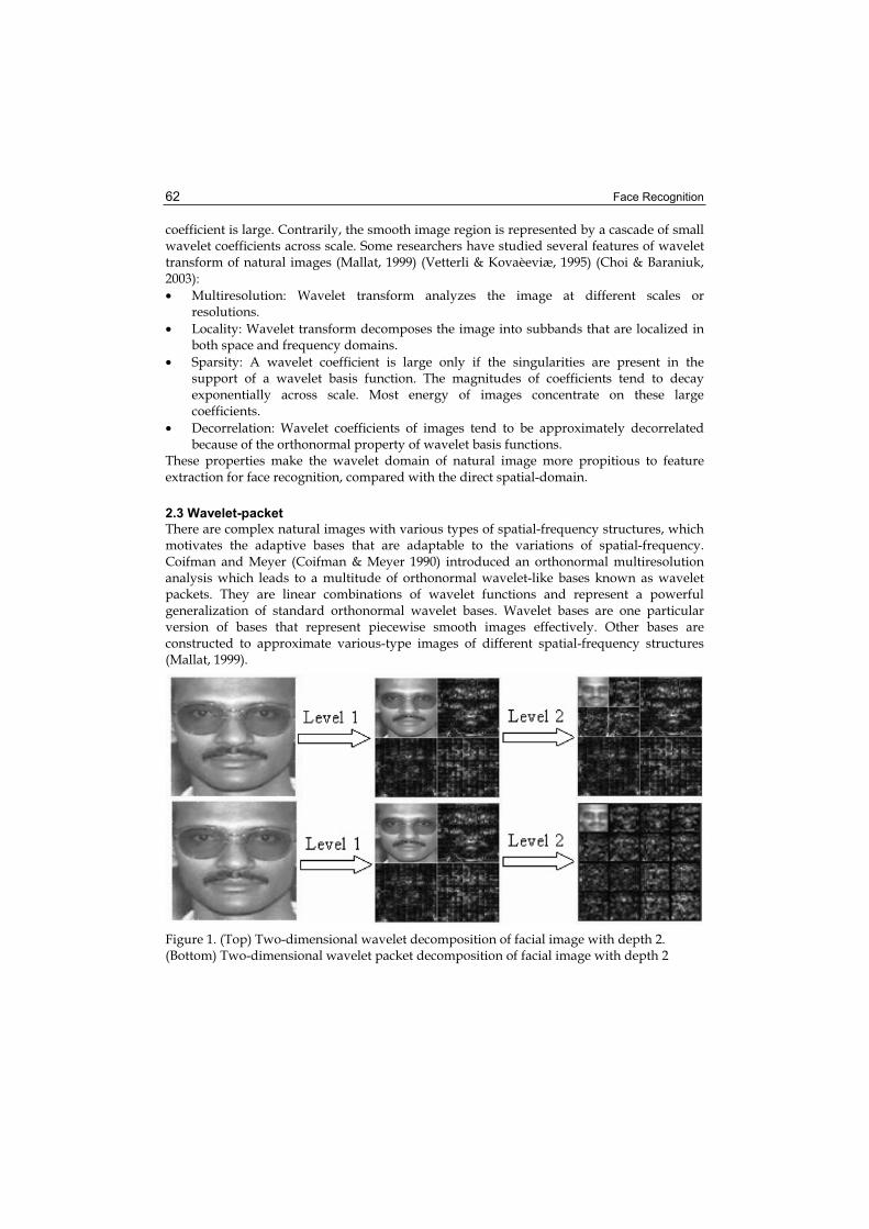
Face Recognition 62
coefficient is large. Contrarily, the smooth image region is represented by a cascade of small wavelet coefficients across scale. Some researchers have studied several features of wavelet transform of natural images (Mallat, 1999) (Vetterli & Kovaèeviæ, 1995) (Choi & Baraniuk, 2003):• Multiresolution: Wavelet transform analyzes the image at different scales or
resolutions.• Locality: Wavelet transform decomposes the image into subbands that are localized in
both space and frequency domains. • Sparsity: A wavelet coefficient is large only if the singularities are present in the
support of a wavelet basis function. The magnitudes of coefficients tend to decay exponentially across scale. Most energy of images concentrate on these large coefficients.
• Decorrelation: Wavelet coefficients of images tend to be approximately decorrelated because of the orthonormal property of wavelet basis functions.
These properties make the wavelet domain of natural image more propitious to feature extraction for face recognition, compared with the direct spatial-domain.
2.3 Wavelet-packet
There are complex natural images with various types of spatial-frequency structures, which motivates the adaptive bases that are adaptable to the variations of spatial-frequency. Coifman and Meyer (Coifman & Meyer 1990) introduced an orthonormal multiresolution analysis which leads to a multitude of orthonormal wavelet-like bases known as wavelet packets. They are linear combinations of wavelet functions and represent a powerful generalization of standard orthonormal wavelet bases. Wavelet bases are one particular version of bases that represent piecewise smooth images effectively. Other bases are constructed to approximate various-type images of different spatial-frequency structures (Mallat, 1999).
Figure 1. (Top) Two-dimensional wavelet decomposition of facial image with depth 2. (Bottom) Two-dimensional wavelet packet decomposition of facial image with depth 2

Wavelets and Face Recognition 63
As a generalization of the wavelet transform, the wavelet packet coefficients also can be computed with two-channel filter bank algorithm. The two-channel filter bank is iterated over both the lowpass and highpass branch in wavelet packet decomposition. Not only L1 is further decomposed as in wavelet decomposition, but also H1, V1, D1 are further decomposed. This provides a quad-tree structure corresponding to a library of wavelet packet basis and images are decomposed into both spatial and frequency subbands, as shown in Fig 1.
3. Preprocessing: Denoising
Denoising is an important step in the analysis of images (Donoho & Johnstone 1998, Starck et al. 2002). In signal denoising, a compromise has to be made between noise reduction and preserving significant signal details. Denoising with the wavelet transform has been proved to be effective, especially the nonlinear threshold-based denoising schemes. Wavelet Transform implements both low-pass and high-pass filters to the signal. The low-frequency parts reflect the signal information, and the high-frequency parts reflect the noise and the signal details. Thresholding to the decomposited high-frequency coefficients on each level can effectively denoise the signal. Generally, denoising with wavelet consists of three steps: • Wavelet Decomposition. Transform the noisy data into wavelet domain. • Wavelet Thresholding. Apply soft or hard thresholding to the high-frequency
coefficients, thereby suppress those coefficients smaller than certain amplitude. • Reconstruction. Transform back into the original domain. In the whole process, a suitable wavelet, an optimal decomposition level for the hierarchy and one appropriate thresholding function should be considered (Mallat 1999). But the choice of threshold is the most critical.
3.1 Wavelet Thresholding
Assuming the real signal f [n] of size N is contaminated by the addition of a noise. This noise is modeled as the realization of a random process W[n]. The observed signal is
The signal f is estimated by transforming the noisy data X with a decision operator Q. The resulting estimator is
The goal is to minimize the error of the estimation, which is measured by a loss function. The square Euclidean norm is a familiar loss function. The risk of the estimator of f is the average loss:
The noisy data
X = f + W (3)
is decomposed in a wavelet basis . The inner product of (3) with bm gives

Face Recognition 64
where .A diagonal estimator of f from (3) can be written
where m are thresholding functions. A wavelet thresholding is equivalent to estimating the signal by averaging it with a kernel that is locally adapted to the signal regularity. A filter bank of conjugate mirror filters decomposes a discrete signal in a discrete orthogonal wavelet basis. The discrete wavelets
are translated modulo modifications near the boundaries. The support of the signal is normalized to [0, 1] and has N samples spaced by N–1. The scale parameter 2j thus varies from 2L = N–1 up to 2J <1:
A thresholding estimator in this wavelet basis can be written
where T is a hard thresholding or a soft thresholding. A hard thresholding estimator is implemented with
A soft thresholding estimator is implemented with
The threshold T is generally chosen so that there is a high probability that it is just above the maximum level of the noise. When WB is a vector of independent Gaussian random variables of variance 2 , the maximum amplitude of the noise has a very high probability of being just below . So we often choose the threshold . In this case, the soft thresholding guarantees with a high probability that
. The estimator is at least as regular as f because its wavelet coefficients have a smaller amplitude. This is not true for the hard thresholding estimator, which leaves unchanged the coefficients above T , and which can therefore be larger than those of f because of the additive noise component. Face images with noise can be estimated by thresholding their wavelet coefficients. The image f [n1, n2] contaminated by a white noise is decomposed in a separable two-dimensional wavelet basis. Figure 2 (a) is the original image, Figure 2 (b) is the noise image. Figure 2 (c, d) are obtained with a hard thresholding and a soft thresholding in a Symmlet 4 wavelet basis.
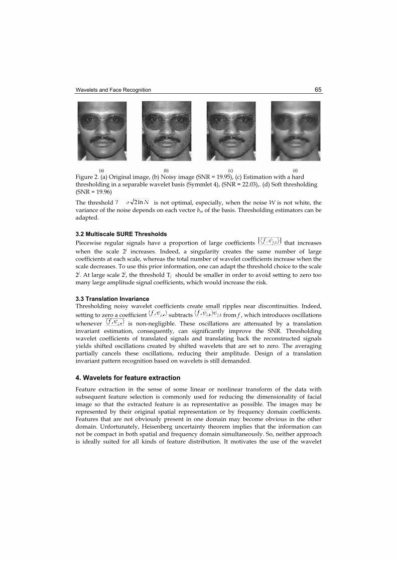
Wavelets and Face Recognition 65
Figure 2. (a) Original image, (b) Noisy image (SNR = 19.95), (c) Estimation with a hard thresholding in a separable wavelet basis (Symmlet 4), (SNR = 22.03),. (d) Soft thresholding (SNR = 19.96)
The threshold is not optimal, especially, when the noise W is not white, the variance of the noise depends on each vector bm of the basis. Thresholding estimators can be adapted.
3.2 Multiscale SURE Thresholds
Piecewise regular signals have a proportion of large coefficients that increases when the scale 2j increases. Indeed, a singularity creates the same number of large coefficients at each scale, whereas the total number of wavelet coefficients increase when the scale decreases. To use this prior information, one can adapt the threshold choice to the scale 2j. At large scale 2j, the threshold Tj should be smaller in order to avoid setting to zero too many large amplitude signal coefficients, which would increase the risk.
3.3 Translation Invariance
Thresholding noisy wavelet coefficients create small ripples near discontinuities. Indeed, setting to zero a coefficient subtracts from f , which introduces oscillations whenever is non-negligible. These oscillations are attenuated by a translation invariant estimation, consequently, can significantly improve the SNR. Thresholding wavelet coefficients of translated signals and translating back the reconstructed signals yields shifted oscillations created by shifted wavelets that are set to zero. The averaging partially cancels these oscillations, reducing their amplitude. Design of a translation invariant pattern recognition based on wavelets is still demanded.
4. Wavelets for feature extraction
Feature extraction in the sense of some linear or nonlinear transform of the data with subsequent feature selection is commonly used for reducing the dimensionality of facial image so that the extracted feature is as representative as possible. The images may be represented by their original spatial representation or by frequency domain coefficients. Features that are not obviously present in one domain may become obvious in the other domain. Unfortunately, Heisenberg uncertainty theorem implies that the information can not be compact in both spatial and frequency domain simultaneously. So, neither approach is ideally suited for all kinds of feature distribution. It motivates the use of the wavelet
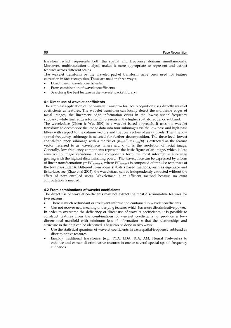
Face Recognition 66
transform which represents both the spatial and frequency domain simultaneously. Moreover, multiresolution analysis makes it more appropriate to represent and extract features across different scales. The wavelet transform or the wavelet packet transform have been used for feature extraction in face recognition. These are used in three ways: • Direct use of wavelet coefficients. • From combination of wavelet coefficients. • Searching the best feature in the wavelet packet library.
4.1 Direct use of wavelet coefficients
The simplest application of the wavelet transform for face recognition uses directly wavelet coefficients as features. The wavelet transform can locally detect the multiscale edges of facial images, the lineament edge information exists in the lowest spatial-frequency subband, while finer edge information presents in the higher spatial-frequency subband. The waveletface (Chien & Wu, 2002) is a wavelet based approach. It uses the wavelet transform to decompose the image data into four subimages via the low-pass and high-pass filters with respect to the column vectors and the row vectors of array pixels. Then the low spatial-frequency subimage is selected for further decomposition. The three-level lowest spatial-frequency subimage with a matrix of (nrow/8) x (ncol/8) is extracted as the feature vector, referred to as waveletface, where nrow x ncol is the resolution of facial image. Generally, low frequency components represent the basic figure of an image, which is less sensitive to image variations. These components form the most informative subimage gearing with the highest discriminating power. The waveletface can be expressed by a form of linear transformation: y= WTwavelet x, where WTwavelet x is composed of impulse responses of the low pass filter h. Different from some statistics based methods, such as eigenface and fisherface, see (Zhao et al 2003), the waveletface can be independently extracted without the effect of new enrolled users. Waveletface is an efficient method because no extra computation is needed.
4.2 From combinations of wavelet coefficients
The direct use of wavelet coefficients may not extract the most discriminative features for two reasons: • There is much redundant or irrelevant information contained in wavelet coefficients. • Can not recover new meaning underlying features which has more discriminative power. In order to overcome the deficiency of direct use of wavelet coefficients, it is possible to construct features from the combinations of wavelet coefficients to produce a low-dimensional manifold with minimum loss of information so that the relationships and structure in the data can be identified. These can be done in two ways: • Use the statistical quantum of wavelet coefficients in each spatial-frequency subband as
discriminative features. • Employ traditional transforms (e.g., PCA, LDA, ICA, AM, Neural Networks) to
enhance and extract discriminative features in one or several special spatial-frequency subbands.

Wavelets and Face Recognition 67
4.2.1 Use the statistical measures as discriminative features
The statistical measures, e. g., mean, variance, are usually helpful to represent features or characteristics of data, it is simple and requires less computation load. Garcia et al. (Garcia et al., 1998) present a wavelet-based framework for face recognition. Each face is described by a subset of subband filtered images containing wavelet coefficients after two-level wavelet packet transform. These coefficients characterize the face texture and a set of simple statistical measures are used to reduce dimensionality and characterize
textural information, which forms compact and meaningful feature vectors .After the extraction of all the vectors of the training set, only the components with a mean value above a predefined threshold are considered for feature vector formation. It is supposed that each component pair is independent from the other component pairs of the feature vector. Then, the Bhattacharrya distance between two feature vectors k and l is computed on a component-pair basis
in order to classify the face feature vectors into person classes. In fact, other statistical measures, e. g., other kinds of moments can be used in the above wavelet-based framework for face recognition. Moreover, the discrete density function of whole wavelet coefficients in each subband can be evaluated. The similarity measure of density function can be computed by some relative entropy, such as Kullback-Leibler divergence or J-divergence.
4.2.2 Employ traditional transform in special subbands
Generally, the wavelet coefficients are deficient to be good discriminative features, a further discriminant analysis is adopted to recover new meaningful underlying features which has more discriminative power. The traditional transforms (e.g., PCA, LDA, ICA, AM, Neural Networks) are very popular for their simplicity and practicality. They can be performed on one or several special spatial-frequency subbands which may be chosen by certain criterion. We (Feng et al. 2000) proposed a wavelet subband approach in using PCA for human face recognition. Three-level wavelet transform is adopted to decompose an image into different subbands with different frequency components. A midrange frequency subband is selected for PCA representation. The experiments show that it has low computation and higher accuracy, comparing with using original PCA directly in spatial domain. In (Dai & Yuen, 2006) we used a wavelet enhanced regularized discriminant analysis to solve the small sample size problem and applied it to human face recognition. We analyzed the role of the wavelet transform, low-pass filtering will reduce the dimension of input data but meanwhile increases the magnitude of the within-class covariance matrix so that the variation information plays too strong a role and the performance of the system will become poorer. It also overcomes the difficulty in solving a singular eigenvalue problem in traditional LDA. Moreover, a wavelet enhanced regularization LDA system for human face recognition is proposed to adequately utilize the information in the null space of withinclass scatter matrix (Dai & Yuen, 2003). Ekenel et al. (Ekenel & Sankur, 2005) introduced a ternary-architecture multiresolution face recognition system. They used the 2D discrete wavelet transform to extract multiple

Face Recognition 68
subband face images. These subband images contain coarse approximations of the face as well as horizontal, vertical and diagonal details of faces at various scales. Subsequently, The PCA or ICA features are extracted from these subbands. They exploit these multiple channels by fusing their information for improved recognition. Their experiments show that it has good performance, especially against illumination perturbations. In ( Zhang et al., 2004), they proposed a modular face recognition scheme by combining the techniques of wavelet subband representations and kernel associative memories. By the wavelet transform, face images are decomposed and the computational complexity is substantially reduced by choosing a lower spatial-frequency subband image. Then an kernel associative memory (KAM) model are built up for each subject, with the corresponding prototypical images without any counter examples involved. Multiclass face recognition is thus obtained by simply holding these associative memories. When a probe face is presented, the KAM model gives the likelihood that the probe is from the corresponding class by calculating the reconstruction errors or matching scores. Illumination compensation is always a problem important but difficult to solve in face recognition. The wavelet transform decomposes the data into different frequency ranges which allows us to isolate the frequency components introduced by illumination effects into certain subspaces. We can use the subspaces that do not contain these illumination-based frequency components to better represent our data, so as to eliminate the influence of the illumination changes, before a face image is recognized. In (Zhang et al., 2005), a face compensation approach based on wavelet and neural network is proposed. A rough linear illumination compensation was first performed for the given face image, which can only compensate the lower frequency features and the effect is limited. The higher frequency features are not be compensated. But it can reduce the learning pressure of the neural network, accelerate the convergent rate and improve the learning accuracy as well as the extensibility of the network. The method can compensates the different scale features of the face image by using the multi-resolution characteristic of the wavelet and the self-adaptation learning and good spread ability of BP neural network. Their experiments show that it can solve the problem of illumination compensation in the face recognition process.
4.3 Search local discriminant basis/coordinates in wavelet packet library
As a generalization of the wavelet transform, the wavelet packet not only offers us an attractive tool for reducing the dimensionality by feature extraction, but also allows us to create localized subbands of the data in both space and frequency domains. A wavelet packet dictionary provides an over-complete set of spatial-frequency localized basis functions onto which the facial images can be projected in a series of subbands. The main design problem for a wavelet packet feature extractor is to choose which subset of basis functions from the dictionary should be used. Most of the wavelet packet dictionary methods that have been proposed in the literature are based on algorithms which were originally designed for signal compression such as the best basis algorithm (Coifman & Wicherhauser, 1992), or the matching pursuit algorithm (Mallat & Zhang, 1993). Saito and Coifman introduced the local discriminant basis (LDB) algorithm based on a best basis paradigm, searching for the most discriminant subbands (basis) that illuminates the dissimilarities among classes from the wavelet packet dictionary (Coifman & Satio, 1994) (Satio & Coifman, 1995). It first decomposes the facial images in the wavelet packet dictionary, then facial image energies at all coordinates in each subband are accumulated for

Wavelets and Face Recognition 69
each class separately to form a spatial-frequency energy distribution per class on the subband. Then the difference among these energy distributions of each subband is measured by a certain “distance” function (e.g., Kullback-Leibler divergence), a complete local discriminant basis (LDB) is selected by the difference-measure function using the best basis algorithm (Coifman & Wicherhauser, 1992), which can represent the distinguishing facial features among different classes. After the basis is selected, the loadings of their coordinates are fed into a traditional classifier such as linear discriminant analysis (LDA) or classification tree (CT). Finally, the corresponding coefficients of probes are computed and fed to the classifier to predict their classes. Unfortunately, the energies may not be so indicative for discrimination sometimes, because not all coordinates in the LDB are powerful to distinguish different subjects. Many less discriminant coordinates may add up to a large discriminability for the LDB. An example of artificial problem was used to validate that it may be fail to select the right basis function as a discriminator (Saito & Coifman, 2002). So Saito and Coifman suggested a modified version of the LDB (MLDB) algorithm which uses the empirical probability distributions instead of the space-scale energy as their selection strategy to eliminate some less discriminant coordinates in each subband locally (Saito & Coifman, 2002). It estimates the probability density of each class in each coordinate in all subbands. Then the discriminative power of each subband is represented by the first N0 most discriminant coordinates in terms of the “distance” among the corresponding densities (e.g., Kullback-Leibler divergence among the densities). This information is then used for selecting a basis for classification as in original LDB algorithm. Although the MLDB algorithm may overcome some shortage of LDB, the selection of coordinates is only limited to each subband so that the coordinates in different subbands are still incomparable. Therefore, the MLDB algorithm gives an alternative to the original LDB. This LDB concept has become increasingly popular and has been applied to a variety of classification problems. Based on LDB idea, Kouzani et al. proposed a human face representation and recognition system based on the wavelet packet method and the best basis selection algorithm (Kouzani et al. 1997). An optimal transform basis, called the face basis, is identified for a database of the known face images. Then it is used to compress all known faces within the database in a single pass. For face recognition, the probe face image is transformed, and the compressed face is then compared against the database. The best filter and best wavelet packet decomposition level are also discussed there. Since features with good discriminant property may locate in different subbands, it is important to find them among all subbands instead of certain specific subbands. We proposed a novel local discriminant coordinates (LDC) method based on wavelet packet for face recognition to compensate for illumination, pose and expression variations (Liu et al. 2007). The method searches for the most discriminant coordinates from the wavelet packet dictionary, instead of the most discriminant basis as in the LDB algorithm. The LDC idea makes use of the scattered characteristic of best discriminant features. In the LDC method, the feature selection procedure is independent of subbands, and only depends on the discriminability of all coordinates, because any two coordinates in the wavelet packet dictionary are comparable for their discriminability which is computed by a maximum a posterior logistic model based on a dilation invariant entropy. LDC based feature extraction not only selects low frequency components, but also middle frequency components whose judicious combination with low frequency components can improve the performance of face recognition greatly.

Face Recognition 70
4.4 Robust issue
It is known that a good feature extractor of face recognition system is claimed to select as more as possible the best discriminant features which are not sensitive to arbitrary environmental variations. Nastar et al. (Nastar & Ayach, 1996) investigated the relationship between variations in facial appearance and their deformation spectrum. They found that facial expressions and small occlusions affect the intensity manifold locally. Under frequency-based representation, only high-frequency spectrum is affected. Moreover, changes in pose or scale of a face and most illumination variations affect the intensity manifold globally, in which only their low-frequency spectrum is affected. Only a change in face will affect all frequency components. So there are no special subbands whose all coordinates are not sensitive to these variations. In each subband, there may be only segmental coordinates have enough discriminant power to distinguish different person, the remainder may be sensitive to environmental changes, So some methods based on the whole subband may also use these sensitive features which maybe affect their performance for face recognition. Moreover, there may be no special subbands containing all the best discriminant features, because the features not sensitive to environmental variations are always distributed in different coordinates of different subbands locally. So methods based on the segmental subbands may lose some good discriminant features. Furthermore, in different subbands, the amount and distribution of best discriminant coordinates are always different. Many less discriminant coordinates in one subband may add up to a larger discriminability than another subband whose discriminability is added up with few best discriminant coordinates and residual small discriminant coordinates. So the few best discriminant coordinates may be discarded by some methods which search for the best discriminate subbands, but usually only the few best discriminant coordinates are needed.So the best discriminant information selection should be independent of their seated subbands, and only depends on their discriminability for face recognition. In addition, there may be some redundancy or collinearity in features which will affect the performance for face recognition. However, another limitation of using wavelet for face recognition is that the wavelet transform has no property of translation invariance. Mallat (Mallat, 1996) discussed that the wavelet representation not only contains spatial and frequency information, but also phase information. When the phase information varies with small translations, it will cause difficulties with matched filtering applications. For achieving translation invariance, it should contain some redundant information in the representing features.The wide-range variations of human face, due to pose, illumination, and expression, require the wavelet transform to extract features that are translation invariant and to a certain extent scale invariant. This constitutes a trade-off between the amount of possible invariance and the sparseness of the wavelet representation. So a robust wavelet feature extractor should select a best discriminant features group with appropriate redundancy or co-linearity. However, searching such a wavelet feature extractor is a difficult task and needs further research.

Wavelets and Face Recognition 71
5. Conclusion
Wavelets have been successfully used in image processing. Their ability to capture localized spatial-frequency information of image motivates their use for feature extraction. We give an overview of using wavelets in the face recognition technology. Due to limit of space the use of Gabor wavelets is not covered in this survey. Interested readers are referred to section 8.3 for references.
6. Acknowledgements
This project is supported in part by NSF of China (60175031, 10231040, 60575004), the Ministry of Education of China (NCET-04-0791), NSF of GuangDong (05101817) and the Hong Kong Research Grant Council(project CityU 122506).
7. References
Chien, J. T. & Wu, C. C. (2002). Discriminant waveletfaces and nearest feature classifiers for face recognition, IEEE Trans. Pattern Analysis and Machine Intelligence, Vol. 24, No. 12, (Dec. 2002) pp. 1644–1649.
Choi, H. & Baraniuk, R. G. (2003). Wavelet Statistical Models and Besov Spaces, In: Nonlinear Estimation and Classification, Denison, D. D.; Hansen, M. H., et al. (Eds.), pp. 9-29, Springer-Verlag, NewYork.
Coifman, R. R. & Meyer, Y. (1990). Orthonormal wavelet packet bases, Preprint. Coifman, R. R. & Wicherhauser, M. V. (1992). Entropy-based algorithm for best basis
selection, IEEE Trans. Infor. Theory, Vol. 38, No. 2, (March, 1992) pp. 713–718. Dai, D. Q. & Yuen, P. C. (2003). Wavelet-based 2-parameter regularized discriminant
analysis for face recognition, In: AVBPA 2003, LNCS 2688, J. Kittler and M.S. Nixon (Eds.), pp. 137–144, Springer-Verlag, Berlin Heidelberg.
Dai, D. Q. & Yuen, P. C. (2006). Wavelet based discriminant analysis for face recognition, Applied Mathematics and Computation, 175(April 2006), 307-318
Daubechies, I. (1992). Ten Lectures on Wavelets, SIAM, New York, 1992. Donoho D. L. & Johnstone I. M. (1998). Minimax estimation via wavelet shrinkage, Annals of
Statistics, 26 (3) (JUN 1998) pp. 879-921. Ekenel, H. K. & Sanker, B. (2005). Multiresolution face recognition, Image and Vision
Computing, Vol. 23, (May 2005) pp. 469–477. Feng, G. C., Yuen, P. C. & Dai, D. Q. (2000). Human face recognition using PCA on wavelet
subband, Journal of Electronic Imaging, Vol. 9, No. 2, (April 2000) pp. 226–233. Garcia, C., Zikos, G. & Tziritas, G. (1998). A wavelet-based framework for face recognition,
Proc of the Workshop on Advances in Facial Image Analysis and Recognition Technology, 5th European Conference on Computer Vision (ECCV'98) , pp. 84-92, Freiburg Allemagne.
Jain A. K., Ross R. & Prabhakar S. (2004) , An introduction to biometric recognition, IEEE Trans. on Circuits and Systems for Video Technology, Vol. 14, no. 1 (Jan. 2004), pp. 4-20.
Kouzani, A. Z., He, F. & Sammut, K. (1997). Wavelet packet face representation and recognition, IEEE Int Conf. Systems, Man, and Cybernetics, Vol. 2, (Oct. 1997) pp. 1614–1619.

Face Recognition 72
Liu C. C., Dai D. Q. & Yan H. (2007). Local discriminant wavelet packet coordinates for face recognition, Journal of Machine Learning Research, Vol. 8 (May 2007) 1165-1195.
Mallat, S. & Zhang, Z. (1993). Matching pursuit in a time_frequency dictionary, IEEE Transactions on Signal Processing, Vol. 41, pp. 3397–3415.
Mallat, S. (1996). Wavelets for a vision, Proc. IEEE, Vol. 84, No. 4, pp. 604-614. Mallat, S. (1999). A Wavelet Tour of Signal Processing, Academic Press (2nd Edition), ISBN : 0-
12-466606-X , San Diego. Nastar, C. & Ayach, N. (1996). Frequency-based nonrigid motion analysis, IEEE Trans.
Pattern Analysis and Machine Intelligence, Vol. 18, (Nov. 1996) pp. 1067–1079. Saito, N. & Coifman, R. R. (1994). Local discriminant bases, Proc. SPIE 2303, pp 2–14. Saito, N. & Coifman, R. R. (1995). Local discriminant bases and their applications, J. Math,
Imaging Vision, Vol. 5, No. 4, pp. 337–358. Saito, N., Coifman, R. R., Geshwind, F. B. & Warner, F. (2002). Discriminant feature
extraction using empirical probability density estimation and a local basis library, Pattern Recognition, Vol. 35, (Dec. 2002) pp. 2841–2852.
Starck J. L., Candes E. J. , Donoho D. L. (2002). The curvelet transform for image denoising, IEEE Transactions on Image Processing 11 (6)( JUN 2002) pp. 670-684
Vetterli, M. & Kovaèeviæ, J. (1995). Wavelets and Subband coding, Prentice Hall, Englewood Cliffs, NJ.
Zhang, B. L., Zhang, H. H. & Ge, S. S. (2004). Face recognition by applying wavelet subband representation and kernel associative memory, IEEE Trans. Neural Networks, Vol. 15, No. 1, (Jan 2004) pp. 166–177.
Zhang, Z. B., Ma, S. L. & Wu, D. Y. (2005). The application of neural network and wavelet in human face illumination compensation, Proc. Advances in Neural Networks, pp. 828– 835.
Zhao W., Chellappa R. Phillips P. J. & Rosenfeld A. (2003). Face recognition: A literature survey, ACM Comput. Surv. Vol. 35, no. 4, (Dec. 2003) pp. 399-459.
8. Further readings
8.1 Face detection
Huang, L. L. & Shimizu, A. (2006). A multi-expert approach for robust face detection, Pattern Recognition, Vol. 39, No. 9, (SEP 2006) pp. 1695-1703.
Liu, C. J. (2003). A Bayesian discriminating features method for face detection, IEEE Transactions on Pattern Analysis and Machine Intelligence, Vol. 25, No. 6, (JUN 2003) pp. 725-740.
Le, D. D. & Satoh, S. (2006). A multi-stage approach to fast face detection, IEICE Transactions on Information and Systems, E89D No. 7, (JUL 2006) pp. 2275-2285.
Shih, P. C. & Liu, C. J. (2006). Face detection using discriminating feature analysis and Support Vector Machine, Pattern Recognition, Vol. 39, No. 2, (FEB 2006) pp. 260-276.
Wang, J. W. & Chen, W. Y. (2006). Eye detection based on head contour geometry and wavelet subband projection, Optical Engineering, Vol. 45, No. 5, (MAY 2006).

Wavelets and Face Recognition 73
8.2 Face recognition
Bebis, G.; Gyaourova, A.; Singh, S. & Pavlidis, I. (2006). Face recognition by fusing thermal infrared and visible imagery, Image and Vision Computing, Vol. 24, No. 7, (JUL 2006) pp. 727-742.
Kwak, K. C. & Pedrycz, W. (2004). Face recognition using fuzzy integral and wavelet decomposition method, IEEE Transactions On Systems Man And Cybernetics Part B Cybernetics, Vol. 34, No. 4, (AUG 2004) pp. 1666-1675.
Kruger, V. & Sommer, G. (2002). Wavelet networks for face processing, Journal of the Optical Society of America A-Optics Image Science and Vision, Vol. 19, No. 6, (JUN 2002) pp. 1112-1119.
Li, B. & Liu, Y. H. (2002). When eigenfaces are combined with wavelets, Knowledge-Based Systems, Vol. 15, No. 5-6, JUL 2002 pp. 343-347.
Ngo, D. C. L.; Teoh, A. B. J. & Goh, A. (2006). Biometric hash: High-confidence face recognition, IEEE Transactions on Circuits and Systems for Video Technology, Vol. 16, No. 6 (JUN 2006) pp. 771-775.
Pal, H. S.; Ganotra, D. & Neifeld, M. A. (2005). Face recognition by using feature-specific imaging, Applied Optics, Vol. 44, No. 18, (JUN 2005) pp. 3784-3794.
Perlibakas, V. (2004). Face recognition using principal component analysis and wavelet packet decomposition, Informatica, Vol. 15, No. 2, pp. 243-250.
Rajwade, A. & Levine, M. D. (2006). Facial pose from 3D data, Image and Vision Computing,Vol. 24, No. 8, (AUG 2006) pp. 849-856.
Shih, F. Y. & Cheng, S. X. (2005). Improved feature reduction in input and feature spaces, Pattern Recognition, Vol. 38, No. 5, (MAY 2005) pp. 651-659. Wavelets and face recognition 17
Tay, D. B. H. (2002). Parametric Bernstein polynomial for least squares design for all other of 3-D wavelet filter banks, IEEE Transactions on Circuits and Systems I-Fundamental Theory and Applications, Vol. 49, No. 6, (JUN 2002) pp. 887-891.
Wijaya, S. L.; Savvides, M. & Kumar, B. V. K. V. (2005). Illumination-tolerant face verification of low-bit-rate JPEG2000 wavelet images with advanced correlation filters for handheld devices, Applied Optics, Vol. 44, No. 5, (FEB 2005) pp. 655-665.
8.3 Using Gabor wavelets
Arca, S.; Campadelli, P. & Lanzarotti, R. (2006). A face recognition system based on automatically determined facial fiducial points, Pattern Recognition, Vol. 39, No. 3, (MAR 2006) pp. 432-443.
Gokberk, B.; Irfanoglu, M. O.; Akarun, L. & Alpaydin, E. (2005). Selection of location, frequency, and orientation parameters of 2D Gabor wavelets for face recognition, Advanced Studies in Biometrics, Vol. 3161, pp. 138-146.
Jeon, I. J.; Nam, M. Y. & Rhee, P. K. (2005). Adaptive gabor wavelet for efficient object recognition, Knowledge-Based Intelligent Information and Engineering Systems, Part 2, Vol. 3682, pp. 308-318.
Kamarainen, J. K.; Kyrki, V. & Kalviainen, H. (2006). Invariance properties of Gabor filterbased features - Overview and applications, IEEE Transactions on Image Processing, Vol. 15, No. 5, (MAY 2006) pp. 1088-1099.

Face Recognition 74
Kim, D. S.; Jeon, I.; Lee, S. Y.; Rhee, P. K. & Chung, D. J. (2006). Embedded face recognition based on fast genetic algorithm for intelligent digital photography, IEEETransactions on Consumer Electronics, Vol. 52, No. 3, (AUG 2006) pp. 726-734.
Liu, C. J. & Wechsler, H. (2002). Gabor feature based classification using the enhanced Fisher linear discriminant model for face recognition, IEEE Transactions on Image Processing, Vol. 11, No. 4, (APR 2002) pp. 467-476.
Liu, C. J. & Wechsler, H. (2003). Independent component analysis of Gabor feature's for face recognition, IEEE Transactions on Neural Networks, Vol. 14, No. 4, (JUL 2003) pp. 919-928.
Liu, C. J. (2004). Gabor-based kernel PCA with fractional power polynomial models for face recognition, IEEE Transactions on Pattern Analysis and Machine Intelligence, Vol. 26, No. 5, (MAY 2004) pp. 572-581.
Shen, L. L. & Bai, L. (2006). A review on Gabor wavelets for face recognition, Pattern Analysis and Applications, Vol. 9(2-3)(Oct. 2006), pp. 273-292.
Shin, H. C.; Choi, H. C. & Kim, S. D. (2006). Directionally classified eigenblocks for localized feature analysis in face recognition, Optical Engineering, Vol. 45, No. 7, (JUL 2006).
Singh, R.; Vatsa, M. & Noore, A. (2005). Textural feature based face recognition for single training images, Electronics Letters, Vol. 41, No. 11, (MAY 2005) pp. 640-641.
Yan, S. C.; He, X. F.; Hu, Y. X.; Zhang, H. J.; Li, M. J. & Cheng, Q. S. (2004). Bayesian shape localization for face recognition using global and local textures, IEEE Transactions on Circuits and Systems for Video Technology, Vol. 14, No. 1, (JAN 2004) pp. 102-113.
Yu, J. G. & Bhanu, B. (2006). Evolutionary feature synthesis for facial expression recognition, Pattern Recognition Letters, Vol. 27, No. 11, (AUG 2006) pp. 1289-1298.
Yu, W. W.; Teng, X. L. & Liu, C. Q. (2006). Face recognition fusing global and local features, Journal of Electronic Imaging, Vol. 15, No. 1, (JAN-MAR 2006).
Zhang, H. H.; Zhang, B. L.; Huang, W. M. & Tian, Q. (2005). Gabor wavelet associative memory for face recognition, IEEE Transactions on Neural Networks, Vol. 16, No. 1, (JAN 2005) pp. 275-278.
Zheng, W. M.; Zhou, X. Y.; Zou, C. R. & Zhao, L. (2006). Facial expression recognition using kernel canonical correlation analysis (KCCA), IEEE Transactions on Neural Networks,Vol. 17, No. 1, (JAN 2006) pp. 233-238.

5
Image Compression Effects in Face Recognition Systems
Kresimir Delac, Mislav Grgic and Sonja Grgic University of Zagreb, Faculty of Electrical Engineering and Computing, Zagreb
Croatia
1. Introduction
With the growing number of face recognition applications in everyday life, image- and video-based recognition methods are becoming important research topic (Zhao et al., 2003). Effects of pose, illumination and expression are issues currently most studied in face recognition. So far, very little has been done to investigate the effects of compression on face recognition, even though the images are mainly stored and/or transported in a compressed format. Still-to-still image experimental setups are often researched, but only in uncompressed image formats. Still-to-video research (Zhou et al., 2003) mostly deals with issues of tracking and recognizing faces in a sense that still uncompressed images are used as a gallery and compressed video segments as probes. In this chapter we analyze the effects that standard image compression methods - JPEG (Wallace, 1991) and JPEG2000 (Skodras et al., 2001) - have on three well known subspace appearance-based face recognition algorithms: Principal Component Analysis - PCA (Turk & Pentland, 1991), Linear Discriminant Analysis - LDA (Belhumeur et al., 1996) and Independent Component Analysis - ICA (Bartlett et al., 2002). We use McNemar's hypothesis test (Beveridge et al., 2001; Delac et al., 2006) when comparing recognition accuracy in order to determine if the observed outcomes of the experiments are statistically important or a matter of chance. Following the idea of a reproducible research, a comprehensive description of our experimental setup is given, along with details on the choice of images used in the training and testing stage, exact preprocessing steps and recognition algorithms parameters setup. Image database chosen for the experiments is the grayscale portion of the FERET database (Phillips et al., 2000) and its accompanying protocol for face identification, including standard image gallery and probe sets. Image compression is performed using standard JPEG and JPEG2000 coder implementations and all experiments are done in pixel domain (i.e. the images are compressed to a certain number of bits per pixel and then uncompressed prior to use in recognition experiments). The recognition system's overall setup we test is twofold. In the first part, only probe images are compressed and training and gallery images are uncompressed (Delac et al., 2005). This setup mimics the expected first step in implementing compression in real-life face recognition applications: an image captured by a surveillance camera is probed to an existing high-quality gallery image. In the second part, a leap towards justifying fully compressed domain face recognition is taken by using compressed images in both training
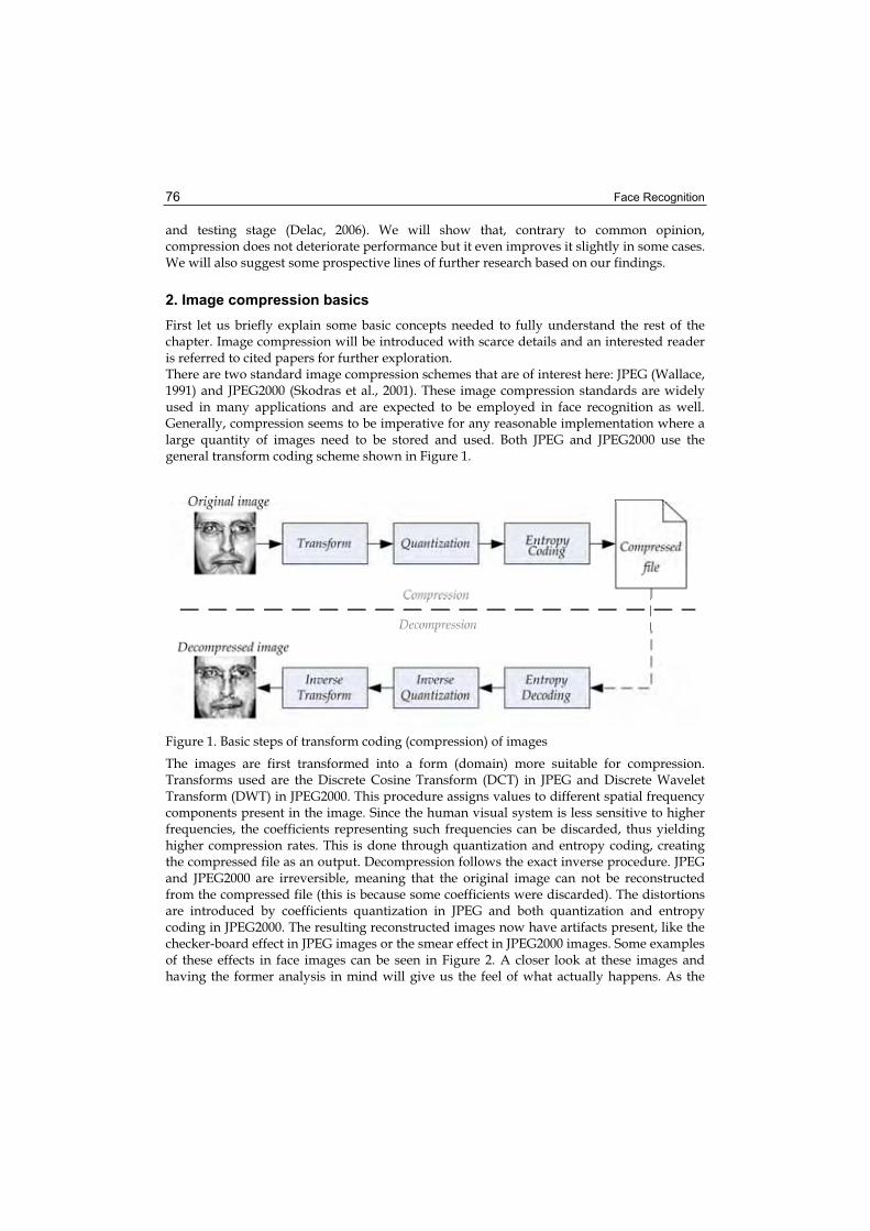
Face Recognition 76
and testing stage (Delac, 2006). We will show that, contrary to common opinion, compression does not deteriorate performance but it even improves it slightly in some cases. We will also suggest some prospective lines of further research based on our findings.
2. Image compression basics
First let us briefly explain some basic concepts needed to fully understand the rest of the chapter. Image compression will be introduced with scarce details and an interested reader is referred to cited papers for further exploration. There are two standard image compression schemes that are of interest here: JPEG (Wallace, 1991) and JPEG2000 (Skodras et al., 2001). These image compression standards are widely used in many applications and are expected to be employed in face recognition as well. Generally, compression seems to be imperative for any reasonable implementation where a large quantity of images need to be stored and used. Both JPEG and JPEG2000 use the general transform coding scheme shown in Figure 1.
Figure 1. Basic steps of transform coding (compression) of images
The images are first transformed into a form (domain) more suitable for compression. Transforms used are the Discrete Cosine Transform (DCT) in JPEG and Discrete Wavelet Transform (DWT) in JPEG2000. This procedure assigns values to different spatial frequency components present in the image. Since the human visual system is less sensitive to higher frequencies, the coefficients representing such frequencies can be discarded, thus yielding higher compression rates. This is done through quantization and entropy coding, creating the compressed file as an output. Decompression follows the exact inverse procedure. JPEG and JPEG2000 are irreversible, meaning that the original image can not be reconstructed from the compressed file (this is because some coefficients were discarded). The distortions are introduced by coefficients quantization in JPEG and both quantization and entropy coding in JPEG2000. The resulting reconstructed images now have artifacts present, like the checker-board effect in JPEG images or the smear effect in JPEG2000 images. Some examples of these effects in face images can be seen in Figure 2. A closer look at these images and having the former analysis in mind will give us the feel of what actually happens. As the
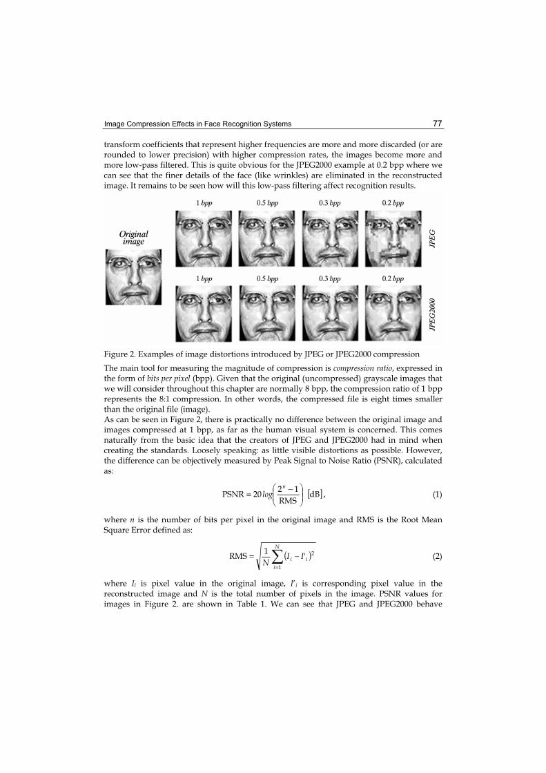
Image Compression Effects in Face Recognition Systems 77
transform coefficients that represent higher frequencies are more and more discarded (or are rounded to lower precision) with higher compression rates, the images become more and more low-pass filtered. This is quite obvious for the JPEG2000 example at 0.2 bpp where we can see that the finer details of the face (like wrinkles) are eliminated in the reconstructed image. It remains to be seen how will this low-pass filtering affect recognition results.
Figure 2. Examples of image distortions introduced by JPEG or JPEG2000 compression
The main tool for measuring the magnitude of compression is compression ratio, expressed in the form of bits per pixel (bpp). Given that the original (uncompressed) grayscale images that we will consider throughout this chapter are normally 8 bpp, the compression ratio of 1 bpp represents the 8:1 compression. In other words, the compressed file is eight times smaller than the original file (image). As can be seen in Figure 2, there is practically no difference between the original image and images compressed at 1 bpp, as far as the human visual system is concerned. This comes naturally from the basic idea that the creators of JPEG and JPEG2000 had in mind when creating the standards. Loosely speaking: as little visible distortions as possible. However, the difference can be objectively measured by Peak Signal to Noise Ratio (PSNR), calculated as:
[ ]dBRMS
1220PSNR −=n
log , (1)
where n is the number of bits per pixel in the original image and RMS is the Root Mean Square Error defined as:
( )=
−=N
iii 'II
N1
21RMS (2)
where Ii is pixel value in the original image, I’i is corresponding pixel value in the reconstructed image and N is the total number of pixels in the image. PSNR values for images in Figure 2. are shown in Table 1. We can see that JPEG and JPEG2000 behave

Face Recognition 78
similarly at moderate compression rates (1 bpp and 0.5 bpp). More apparent differences arise at higher compression rates (0.3 bpp and 0.2 bpp), where JPEG2000 is clearly superior.
1 bpp 0.5 bpp 0.3 bpp 0.2 bpp
JPEG 34.02 30.00 26.30 19.88
JPEG2000 35.96 30.28 28.12 25.96
Table 1. PSNR values in dB for images in Figure 2
Similar conclusions on JPEG and JPEG2000 efficiency can be found in (Grgic et al., 2001). Through using additional objective image quality measures it was shown that DCT-based and DWT-based compression yield similar results at lower compression rates. At higher compression rates, DWT-based compression retains rather high quality while DCT-based compression quality deteriorates rapidly. In (Ebrahimi et al., 2004) authors showed that there is no significant difference in the quality of JPEG and JPEG2000 compressed images at lower and moderate compression rates. JPEG2000 was determined to be superior at higher compression rates. In (Santa-Cruz et al., 2000) authors concluded that JPEG2000 is both subjectively and objectively superior to JPEG. In the literature review that follows, we will see how compression effects were tested in face recognition so far and what still remains to be done.
3. Related work
Before proceeding to related work review, one basic term should be clarified. It has to emphasized that all the experiments described in this chapter, including the ones in the following literature review, are conducted in pixel domain. This actually means that the images are compressed and then uncompressed prior to being used in the experiments. This way the actual influence that the distortion introduced by compression has on recognition rate is measured. There has been little investigation of the effects of image compression on face recognition systems do far. As will be seen, mostly JPEG compression is covered and mainly at a single compression ratio. In (Blackburn et al., 2001) the authors tried to measure the effects of image compression on face recognition systems by simulating the expected real-life setup: images of persons known to the system (gallery) were of high quality (non-compressed) and images of persons unknown to the system (probes) were taken in uncontrolled environment and compressed. Naturally, images were decompressed prior to recognition and thus we can say that experiments were conducted in the pixel domain. JPEG compression was used and face recognition system was tested using the FERET database and its dup1 (temporal changes) probe set. Images were compressed to 0.8, 0.4, 0.25 and 0.2 bpp. The authors conclude that compression does not affect recognition significantly across wide range of compression rates. Significant performance drop is noted at 0.2 bpp and below. Recognition rate is even slightly higher in some cases when using compressed images (compared to results using original images). Moon and Phillips (Moon & Phillips, 2001) tested the effects of standard JPEG compression and of a variant of wavelet compression with a PCA+L1 method. Probe images were in both cases compressed to 0.5 bpp, decompressed (so the experiments were conducted in pixel

Image Compression Effects in Face Recognition Systems 79
domain) and then geometrically normalized. The training set of images was uncompressed. FERET database was used along with its standard probe sets (only fb and dup1 in this experiment). Results indicate no performance drop for JPEG compression and a slight increase for wavelet compression. Whether this increase in recognition rate is significant or not is unclear. JPEG2000 compression effects were tested in (McGarry et al., 2004) as part of the development of the ANSI INCITS 385-2004 standard: "Face Recognition Format for Data Interchange" (ANSI, 2004), later to become an ISO/IEC IS 19794-5 standard: "Biometric Data Interchange Formats - Part 5: Face Image Data" (ISO, 2004). The experiment included compression at a compression rate of 10:1, as recommended in (ANSI, 2004; ISO, 2004). A commercial face recognition system was used for testing a vendor database. Again, since there are no details on the exact face recognition method used in the tested system and no details on a database used in experiments, it is difficult to make any comparisons to this work. In a similar setup as in previously described papers, it was determined that there is no significant performance drop when using compressed probe images. Based on their findings, the authors conjecture that compression rates higher than 10:1 could be used. In (Wat & Srinivasan, 2004) the authors test the effects of JPEG compression on PCA and LDA face recognition methods using the same experimental setup as in (Blackburn et al., 2001). Results are presented as a function of JPEG quality factor. This fact makes any comparison with these results very difficult since the same quality factor will yield different compression rates for different images, dependent upon the statistical properties of a given image. This is why we decided to used bits per pixel as a measure of compression ratio in our experiments. The authors used the FERET database and tested the standard probe sets against a standard gallery. Results indicate a slight increase in performance for the LDA method with the fc probe set. For all other probe sets and methods the results were practically the same as with uncompressed images. An initial detailed experiment of the effects of compression on face recognition was conducted in (Delac et al., 2005). We tested both JPEG and JPEG2000 compression effects on a wide range of subspace algorithm - metric combinations. Similar to other studies, we also concluded that compression does not affect performance significantly. We supported our conclusions with McNemar's hypothesis test. Some performance improvements were also noted, but none of them were statistically significant. Wijaya et al. in (Wijaya et al., 2005) performed face verification on images compressed to 0.5 bpp by JPEG2000 and showed that high recognition rates can be achieved using correlation filters. Their conclusion was also that compression does not adversely effect performance. We can see that the described experiments were mainly done in the same setup: training and gallery images are uncompressed and probe images are compressed to various compression ratios. Most authors conclude that compression does not affect recognition rate significantly, but these conclusions still need to be statistically confirmed. Most of these experiments are limited to a single compression rate and a single recognition method. We will try to address some of these shortcomings in the experiments presented in this chapter.
4. Experimental setups and results
4.1 Database and protocol
We use the standard FERET data set including the data partitions (subsets) for recognition tests, as described in (Phillips et al., 2000). The gallery consists of 1,196 images and there are

Face Recognition 80
four sets of probe images that are compared to the gallery images in recognition stage. The fb probe set contains 1,195 images of subjects taken at the same time as gallery images with the only difference being that the subjects were told to assume a different facial expression. The fc probe set contains 194 images of subjects under different illumination conditions. The dup1 (duplicate I) set contains 722 images taken anywhere between one minute and 1,031 days after the gallery image was taken, and dup2 (duplicate II) set is a subset of dup1containing 234 images taken at least 18 months after the gallery image was taken. All images in the data set are of size 384 × 256 pixels and grayscale.
4.2 Preprocessing
Original FERET images were first spatially transformed (to get the eyes at the predefined fixed points) based upon a ground truth file of the eye coordinates supplied with the original FERET data. All images were then cropped to 128 × 128 pixels (using the eyes coordinates) and an elliptical mask was used to further eliminate the background. Finally, image pixel values were histogram equalized to the range of values from 0 to 255. These preprocessing steps were carried out on all images prior to preforming the experiments (including compression).
4.3 Algorithms
Three well known appearance-based subspace face recognition algorithms were used to test the effects of compression: Principal Component Analysis - PCA (Turk & Pentland, 1991), Linear Discriminant Analysis - LDA (Belhumeur et al., 1996) and Independent Component Analysis - ICA (Bartlett et al., 2002). It is important to mention that we use ICA Architecture 2from (Bartlett et al., 2002) since ICA Architecture 1 was shown to be suboptimal for face identification tasks (Delac et al., 2005; Delac et al. 2006). For both LDA and ICA, a PCA dimensionality reduction was done as a preprocessing step. To train the PCA algorithm we used a subset of classes for which there were exactly three images per class. We found 225 such classes (different persons), so our training set consisted of 3 × 225 = 675 images (M = 675, c = 225). The effect that this percentage of overlap has on algorithm performance needs further exploration and will be part of our future work. PCA derived, in accordance with theory, M - 1 = 674 meaningful eigenvectors. We adopted the FERET recommendation and kept the top 40% of those, resulting in 270-dimensional PCA subspace W (40% of 674 = 270). It was calculated that 97.85% of energy was retained in those 270 eigenvectors. This subspace was used for recognition as PCA face space and as input to ICA and LDA (PCA was the preprocessing dimensionality reduction step). ICA yielded a 270-dimensional subspace, and LDA yielded only 224-dimensional space since it can, by theory, produce a maximum of c - 1 basis vectors. All of those were kept to stay close to the dimensionality of PCA and ICA spaces and thus make comparisons as fair as possible. Based on our previous findings in (Delac et al., 2005; Delac et al., 2006) we chose the following combinations of algorithms and metrics (one metric for each algorithm) to be used in these experiments: PCA+L1, LDA+COS and ICA+COS. These combinations yielded the highest recognition rates in our previous experiments.
4.4 Measurement methods
Performance of face recognition systems (algorithms, methods) will be presented as rank one recognition rate, as described in (Phillips et al., 2000). Let T represent the training set, G

Image Compression Effects in Face Recognition Systems 81
gallery and P probe set of images. T and G can be the same set but this is not a good testing practice. The actual performance of an algorithm is always rated relative to how well the images in P are matched to images in G. This is the basis of automatic face recognition. Intuitively, it is obvious that P and G should be disjoint; otherwise, the stated problem becomes trivial. We will use the identification scenario in our experiments. To calculate the recognition rate for a given probe set P, for each probe image Pi, we need to sort all the gallery images by decreasing similarity, yielding a list L = {L1, L2, ... , LK}, where K is the total number of subjects in the gallery (assuming that there is one image per subject, K also becomes the number of images and the size of the gallery). Now L1 is the gallery image most similar to the given probe image (according to the algorithm), L2 is the next closest match and expanding this to Lk being the kth closest gallery match. Rank one recognition rate answers a simple question: is the top match correct? If L1 (labeled as the closest gallery match to the given probe image) is really the correct answer, we say that the algorithm correctly recognized the probe image. In other words, the algorithm successfully recognizes a probe image if the probe image and the top ranked gallery image in L are of the same subject. This is called rank one recognition rate (RR) and can be formally defined over the whole set of probe images P as follows: let R1 denote the number of correctly recognized probe images in L at k = 1 and |P| be the probe set size, then:
PRRR 1= . (3)
A usual way to report rank one performance is to give it in a form of percentage. That way we actually say that some algorithm has e.g. 86% rank one recognition rate on a given gallery and probe set. Another possible formulation would be that there is 86% chance that the correct answer is the top match (the image L1).To measure the significance of the differences in performance at two different compression ratios, we will use McNemar's hypothesis test (Beveridge et al., 2001; Delac et al., 2006). We think that, when comparing recognition algorithms, it is important (yet often neglected) to answer the following question: when is the observed difference in performance statistically significant? Clearly, the difference in performance of 1% or 2% could be due to pure chance. However, we felt the need to investigate these intuitive presumptions using standard statistical hypothesis testing techniques. Generally, there are two ways of looking at the performance difference (Yambor et al., 2002): 1) determine if the difference (as seen over the entire set of probe images) is significant, 2) when the algorithms behave differently, determine if the difference is significant. As argued in (Yambor et al., 2002), the first way to evaluate performance difference fails to take the full advantage of the standard face recognition protocol, so we will focus on the second way. In order to perform this test we recorded which of the four possible outcomes, when comparing two algorithms A1 and A2 (SS – both successful, FF – both failed, FS – first one failed and the second one succeeded, SF – first one succeeded and the second one failed), is true for each probe image. Let NSS
represent the number of probe images for which SS outcome is true, NSF the number of probe images for which SF outcome is true, etc. We then formulated our hypotheses as: H0) the probability of observing SF is equal to the probability of observing FS; H1) the probability of observing SF is not equal to the probability of observing FS. H0 is the null hypothesis and H1 the alternative hypothesis.

Face Recognition 82
In case where one algorithm performs better than another algorithm, H0 can be rejected if the observed difference in performance of the compared algorithms is statistically significant. Therefore, H0 is tested by applying a one-tailed test. Suppose that Pr(SF) and Pr(FS) are the probabilities of observing SF and FS outcomes under H0. For example, if it appears that Pr(SF) > Pr(FS), i.e. A1 performs better than A2, then we calculate:
Pr (A1 better than A2 at least as many times as observed) = =
⋅−
n
Ni
n
SF)!in(!i
!n21 (4)
where n = NSF + NFS is the number of probe images for which only one algorithm incorrectly classify them. This probability is usually called p-value for rejecting H0 in favor of H1. H0 is rejected when the p-value is lower than some predefined threshold (usually = 0.05, i.e. 5%), and in this case we can conclude that the observed difference in performance of the compared algorithms is statistically significant.We will report the outcomes of McNemar's test in our results as " " when there is no statistically significant difference when using images at a given compression ratio compared to using original images, " " the recognition ratio is significantly worse than with original images and " " when the recognition ratio using compressed images is significantly higher than with original images. Another handy tool that can be used here is the Normalized Recognition Rate (NRR),defined as the ratio between recognition rate (RR) for compressed images and recognition rate for original images (Delac, 2006):
original
compressed
RRRR
NRR = . (5)
So, at a given bitrate (number of bits per pixel), if NRR = 1, the performance is the same as with original images, if NRR < 1, performance is worse, and if NRR > 1, performance is better then with original images. We will present NRR curves (NRR as a function of compression ratio) for some interesting results just as an example of their possible usage. Full analysis of the results with NRR is out of scope of this chapter.
4.5 Experiments
As stated before, most of the experiments presented in the literature so far use the scenario where only probe images are compressed. We will here try to perform another experiment where all the images are compressed to a given compression ratio. This will be a good foundation for possible new area in face recognition research - face recognition in compressed domain. Compressed domain means that instead of decompressing the compressed images and then using (distorted) pixel values as input to face recognition methods, transformed coefficients are used as inputs. The decoding process should be interrupted after the entropy decoding and the obtained coefficients (DCT or DWT) used as inputs to classification methods. This way it is possible to achieve large computational time saves by avoiding the inverse DCT or DWT.
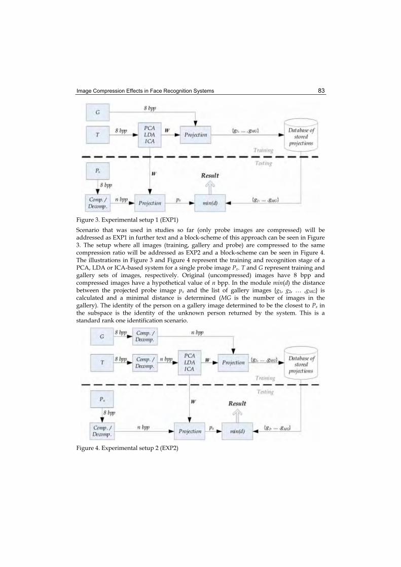
Image Compression Effects in Face Recognition Systems 83
Figure 3. Experimental setup 1 (EXP1)
Scenario that was used in studies so far (only probe images are compressed) will be addressed as EXP1 in further text and a block-scheme of this approach can be seen in Figure 3. The setup where all images (training, gallery and probe) are compressed to the same compression ratio will be addressed as EXP2 and a block-scheme can be seen in Figure 4. The illustrations in Figure 3 and Figure 4 represent the training and recognition stage of a PCA, LDA or ICA-based system for a single probe image Px. T and G represent training and gallery sets of images, respectively. Original (uncompressed) images have 8 bpp and compressed images have a hypothetical value of n bpp. In the module min(d) the distance between the projected probe image px and the list of gallery images {g1, g2, … ,gMG} is calculated and a minimal distance is determined (MG is the number of images in the gallery). The identity of the person on a gallery image determined to be the closest to Px in the subspace is the identity of the unknown person returned by the system. This is a standard rank one identification scenario.
Figure 4. Experimental setup 2 (EXP2)

Face Recognition 84
4.6 Results
The results for both experiments can be seen in Tables 2 through 9. The figures presented on tables represent rank one recognition rates. "McN" presents the result of McNemar's hypothesis test (result at a given compression ratio compared to the result using original uncompressed images). By looking at the results of McNemar’s test, we can immediately conclude that compression to 1 bpp and 0.5 bpp does not significantly influence the results in any method and/or experiment. This is consistent with previous studies and it additionally gives strong statistical basis for such a conclusion. In the following text we will give an analysis for each probe set in both experiments and present two possible real life applications of the conclusions drawn from this study.
fb JPEG Orig. 1 bpp 0.5 bpp 0.3 bpp 0.2 bpp RR 79,4 79,4 79,4 78,9 77,2 EXP1 McN - RR 79.4 78.9 79.4 79.0 75.4
PCA+L1EXP2
McN - RR 75.4 75.4 75.2 75.3 73.6 EXP1 McN - RR 75.4 75.5 75.5 74.5 72.6
LDA+COSEXP2
McN - RR 83.0 82.8 83.0 82.0 80.0 EXP1
McN - RR 83.0 83.1 83.0 82.2 75.6
ICA+COSEXP2
McN -
Table 2. The results for JPEG compression, fb probe set (" " - no statistically significant difference compared to using original images; " " - RR significantly worse than with original images; " " - RR significantly higher than with original images)
fc JPEG Orig. 1 bpp 0.5 bpp 0.3 bpp 0.2 bpp RR 47.9 46.4 45.9 47.9 44.3 EXP1
McN - RR 47.9 50.0 49.5 51.0 42.3
PCA+L1EXP2
McN - RR 11.3 11.3 11.3 11.3 10.8 EXP1
McN - RR 11.3 11.3 11.3 11.9 11.3
LDA+COSEXP2
McN - RR 68.6 68.0 67.5 69.6 66.5 EXP1
McN - RR 68.6 67.5 68.6 66.5 57.7
ICA+COSEXP2
McN -
Table 3. The results for JPEG compression, fc probe set

Image Compression Effects in Face Recognition Systems 85
dup1 JPEG Orig. 1 bpp 0.5 bpp 0.3 bpp 0.2 bpp RR 38.5 38.6 38.5 38.2 35.1 EXP1
McN - RR 38.5 39.2 39.2 38.8 35.7
PCA+L1EXP2 McN -
RR 35.6 35.6 35.3 35.8 33.8 EXP1McN - RR 35.6 35.6 35.3 35.7 33.4
LDA+COSEXP2
McN - RR 44.3 44.9 44.5 42.9 41.1 EXP1
McN - RR 44.3 45.3 44.5 43.6 36.4
ICA+COSEXP2
McN -
Table 4. The results for JPEG compression, dup1 probe set
dup2 JPEG Orig. 1 bpp 0.5 bpp 0.3 bpp 0.2 bpp RR 19.7 20.1 20.1 19.2 15.8 EXP1 McN - RR 19.7 20.5 21.4 19.2 17.2
PCA+L1EXP2
McN - RR 12.8 12.8 12.8 13.6 12.4 EXP1 McN - RR 12.8 13.2 13.2 12.4 13.2
LDA+COSEXP2
McN - RR 30.8 32.0 30.7 29.9 27.3 EXP1 McN - RR 30.8 31.2 30.3 31.2 24.8
ICA+COSEXP2
McN -
Table 5. The results for JPEG compression, dup2 probe set
fb JPEG2000 Orig. 1 bpp 0.5 bpp 0.3 bpp 0.2 bpp RR 79.4 79.4 79.6 79.1 78.6 EXP1 McN - RR 79.4 79.2 79.2 79.7 75.4
PCA+L1EXP2
McN - RR 75.4 75.4 75.3 75.2 75.0 EXP1 McN - RR 75.4 75.5 75.2 75.1 72.6
LDA+COSEXP2
McN - RR 83.0 83.1 83.1 83.0 83.4 EXP1 McN - RR 83.0 83.4 83.5 83.8 76.7
ICA+COSEXP2
McN -
Table 6. The results for JPEG2000 compression, fb probe set

Face Recognition 86
fc JPEG2000 Orig. 1 bpp 0.5 bpp 0.3 bpp 0.2 bpp RR 47.9 46.4 46.4 45.9 45.8 EXP1 McN - RR 47.9 51.0 51.5 52.6 42.3
PCA+L1EXP2
McN - RR 11.3 11.3 11.3 10.8 11.3 EXP1
McN - RR 11.3 11.3 11.3 10.8 11.3
LDA+COSEXP2
McN - RR 68.6 69.0 68.5 68.5 68.6 EXP1
McN - RR 68.6 67.0 67.0 64.4 56.2
ICA+COSEXP2
McN -
Table 7. The results for JPEG2000 compression, fc probe set
dup1 JPEG2000 Orig. 1 bpp 0.5 bpp 0.3 bpp 0.2 bpp RR 38.5 38.3 38.5 38.2 38.5 EXP1
McN - RR 38.5 38.8 38.9 38.0 35.7
PCA+L1EXP2 McN -
RR 35.6 35.6 35.5 35.4 35.1 EXP1McN - RR 35.6 35.5 35.5 35.3 33.4
LDA+COSEXP2 McN -
RR 44.3 44.7 44.5 44.5 44.3 EXP1McN - RR 44.3 45.0 43.8 42.4 35.5
ICA+COSEXP2
McN -
Table 8. The results for JPEG2000 compression, dup1 probe set
dup2 JPEG2000 Orig. 1 bpp 0.5 bpp 0.3 bpp 0.2 bpp RR 19.7 19.7 20.1 19.7 19.6 EXP1 McN - RR 19.7 20.5 19.7 18.8 17.9
PCA+L1EXP2
McN - RR 12.8 13.3 13.7 13.6 13.2 EXP1 McN - RR 12.8 13.2 13.7 13.7 13.2
LDA+COSEXP2
McN - RR 30.8 32.5 32.0 29.5 30.0 EXP1 McN - RR 30.8 32.5 30.8 29.1 22.7
ICA+COSEXP2
McN -
Table 9. The results for JPEG2000 compression, dup2 probe set

Image Compression Effects in Face Recognition Systems 87
5. Analysis
5.1 Different expressions (fb)
All methods exhibit great stability for both JPEG and JPEG2000 compression and in both EXP1 and EXP2 setups (Table 2 and Table 6). Even though there are a few recognition rate increases when the images are mildly compressed, none of those increases are statistically significant. If we take a look at the example of visual deformations introduced by compression (Figure 2), this level of stability is quite surprising. In spite of the fact that an image compressed to 0.3 bpp using JPEG is virtually unrecognizable and, on average, has PSNR = 25 dB, there seems to be no effect on face recognition performance. If we have a closer look at the results in Table 2 and Table 6, we can see that both JPEG and JPEG2000 do not significantly deteriorate performance until 0.2 bpp. At 0.2 bpp all recognition methods experience significant performance drop. We can conclude that, for the different expressions task, all compression ratios above 0.2 bpp are acceptable and can be used in a face recognition system. Unfortunately, rarely are such easy tasks (ideal imaging conditions and face images varying only in facial expressions) put before the systems designers and this is why we have to consider other possible influences on recognition accuracy as well (different illuminations and temporal changes). JPEG2000 seems to be more efficient (in terms of image quality) if an image is to be presented to a human operator that has to make a final decision about someone’s identity. This is an expected scenario in high confidence applications, like law enforcement applications. In such an application, a list of the most likely matches are presented to the user which now has to make the final choice. JPEG2000 images seem to be visually less distorted at higher compression rates and thus more appropriate for such uses. JPEG images can also be used, but at moderate or low compression rates (0.5 bpp and above). The overall rank one recognition rates for the fb probe set are above 75%, which was expected and is consistent with previous studies of the same face recognition algorithms in pixel domain (Delac et al., 2006; Bartlett et al., 2002; Yambor et al., 2002; Beveridge et al., 2001; Belhumeur et al., 1996). ICA+COS yielded highest recognition rates in both experiments. For JPEG - 83% at 0.5 bpp in EXP1 and 83.1% at 1 bpp in EXP2 and for JPEG2000 – 83.1% at 0.5 bpp in EXP1 and 83.8% at 0.3 bpp in EXP2. It is interesting to notice that overall best results was achieved at a surprisingly high compression of 0.3 bpp (≈ 26:1).
5.2 Different illumination (fc)
The results for the fc probe set in both experiments can be seen in Table 3 and 7 and Figure 5 and 6. If we take a look at the results of both experiments for JPEG compression (Table 3 and Figure 5), we can see that compression again does not deteriorate performance up to 0.3 bpp. Only at 0.2 bpp the differences become statistically significant. These results are mainly quite similar to the fb probe set results. However, there are some differences, namely, the statistically significant recognition rate improvement for PCA+L1 with JPEG compression at 0.3 bpp in EXP2, and consistent significant improvement for JPEG2000 compression at 1, 0.5 and 0.3 bpp in EXP2. Both mentioned differences are clearly visible in Figure 5 and 6. In those figures the NRR curves are shown as a function of compression rate (in bpp) for all experiments with the fc probe set (Figure 5 for JPEG and Figure 6 for JPEG2000 compression). As already mentioned, PCA+L1 exhibits some statistically significant improvements in these experiments and this is clearly visible as the curves in Figure 5 and 6
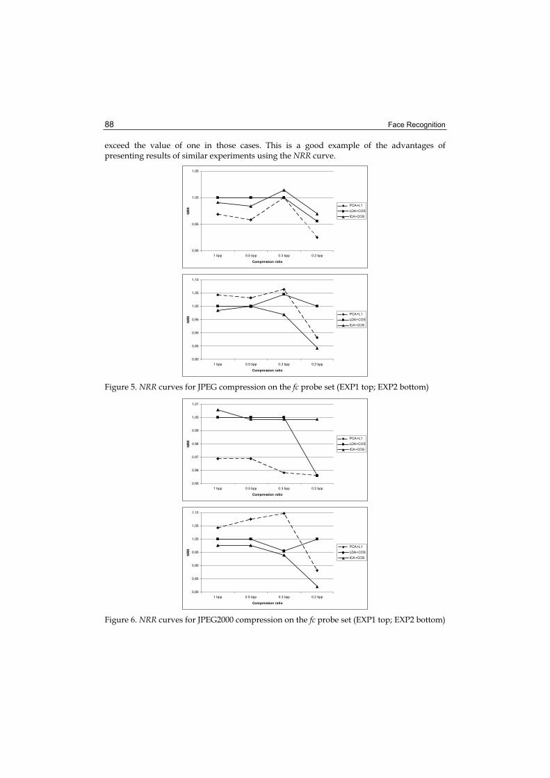
Face Recognition 88
exceed the value of one in those cases. This is a good example of the advantages of presenting results of similar experiments using the NRR curve.
0,90
0,95
1,00
1,05
1 bpp 0.5 bpp 0.3 bpp 0.2 bpp
Compression ratio
NR
R
PCA+L1
LDA+COS
ICA+COS
0,80
0,85
0,90
0,95
1,00
1,05
1,10
1 bpp 0.5 bpp 0.3 bpp 0.2 bpp
Compression ratio
NR
R
PCA+L1
LDA+COS
ICA+COS
Figure 5. NRR curves for JPEG compression on the fc probe set (EXP1 top; EXP2 bottom)
0,95
0,96
0,97
0,98
0,99
1,00
1,01
1 bpp 0.5 bpp 0.3 bpp 0.2 bpp
Compression ratio
NR
R
PCA+L1
LDA+COS
ICA+COS
0,80
0,85
0,90
0,95
1,00
1,05
1,10
1 bpp 0.5 bpp 0.3 bpp 0.2 bpp
Compression ratio
NR
R
PCA+L1
LDA+COS
ICA+COS
Figure 6. NRR curves for JPEG2000 compression on the fc probe set (EXP1 top; EXP2 bottom)

Image Compression Effects in Face Recognition Systems 89
Compression drastically improves the results for PCA+L1 algorithm in some cases. For LDA+COS and ICA+COS this effect is not that emphasized. One might actually expect even worse results for compression of images taken in different illumination conditions. The different illumination influences large portions of an image and sometimes even the whole image. This being so, it appears that illumination changes are represented by low frequencies in an image, thus low-pass filtering (such as JPEG or JPEG2000 compression) should not eliminate the differences between various images taken in different illumination conditions. However, in spite of this, all algorithms seem to be very stable across a wide range of compression rates and in both experimental setups. Nastar et al. (Nastar et al., 1997) showed that only the high-frequency spectrum is affected by changes in facial expression. They also conjecture that illumination changes mostly affect the whole image, thus being in the low-frequency part of the spectrum. It is interesting to notice that PCA+L1 yielded the highest recognition rates for both JPEG and JPEG2000 compression at a very high compression rate of 0.3 bpp. The effect that compression has on PCA+L1 results could be further explored by reconstructing the compressed images after projection to PCA subspace and comparing the reconstructed images to original images to capture the differences induced by compression. The overall best rank one recognition rates for the fc probe set are achieved by ICA+COS in both experiments. For JPEG - 69.6% at 0.3 bpp in EXP1 and 68.6% at 0.5 bpp in EXP2 and for JPEG2000 – 69% at 1 bpp in EXP1 and 67% at 1 and 0.5 bpp in EXP2.
5.3 Temporal changes (dup1 & dup2)
The results for probe sets that test the effect that aging of the subjects has on face recognition (dup1 and dup2) are shown in Tables 4, 5, 8 and 9. The trend of very stable results across a wide range of compression rates is still noticeable. Additionally, for these probe sets all three algorithms have statistically insignificant performance differences, even at 0.2 bpp. Slight (statistically insignificant) improvements are noticeable at almost all compression rates and for all algorithms. It appears that the low-pass filtering by compression contributes more to the overall stability of the results than to significant improvements. The overall best rank one recognition rates for the dup1 probe set are achieved by ICA+COS in both experiments. For JPEG - 44.9% at 1 bpp in EXP1 and 45.3% at 1 bpp in EXP2 and for JPEG2000 – 44.7% at 1 bpp in EXP1 and 45% at 1 bpp in EXP2. The overall best rank one recognition rates for the dup2 probe set are achieved by ICA+COS in both experiments. For JPEG - 32% at 1 bpp in EXP1 and 31.2% at 1 and 0.3 bpp in EXP2 and for JPEG2000 – 32.5% at 1 bpp in EXP1 and 32.5% at 1 bpp in EXP2. Mild compression of 8:1 (1 bpp) seems to be very effective at improving face recognition from images taken at different points in time. The removal of fine details, such as wrinkles and even facial hair, obviously makes images of the same person more similar.
5.4 Possible applications
We will now try to answer a question of where could the results and conclusions presented here be used in real life. We will describe two very basic applications. Firstly, as was previously hinted, the obvious use is in law enforcement applications. An image of an unknown subject is presented to the system, that image is compared to all the images known to the system. There can be hundreds of thousands of such images and any storage requirements save in such application is of crucial importance.

Face Recognition 90
Secondly, there has recently been an increased interest in using face recognition systems in mobile and handheld devices (Wijaya et al., 2005). In such applications the face of the subject is recorded using a camera mounted on a device and transaction/login is approved or rejected based on that image. Recognition is mostly done at the remote server side and images (or some extracted image features) are sent over a telecommunication network. If a device in question is a mobile phone, higher level image processing is usually computationally expensive so the whole image is sent. Cameras usually deliver images in an already compressed format and being able to use this feature and send a compressed file across the network would be a big advantage.
6. Conclusion
We can group the conclusions based on a level of compression and the probe sets into two parts: i) higher compression rates (0.5, 0.3 and in some cases even 0.2 bpp) seem to be suitable for recognizing faces with different expressions (fb probe set) and images taken in different illumination conditions (fc probe set); ii) lower compression rates (1 bpp) seem to be suitable for recognizing images taken at different points in time (dup1 and dup2 probe set). Taking this analysis into account, it seems that the current practice of deciding on the level of compression based on visual distortion of images is wrong. While the images compressed to 0.3 bpp are visually significantly distorted, the recognition results are in almost all experiments statistically indistinguishable from the results achieved by using uncompressed images. In many cases these results are slightly better and in some cases even significantly better than the ones achieved with uncompressed images. The correct criteria for selecting the optimal compression ratio would therefore be: the optimal compression rate is the one yielding the highest recognition rate at given circumstances (classification algorithm, task given etc.). It certainly seems reasonable to allow image compression up to 0.5 bpp (a 16:1 compression) for face recognition purposes. JPEG2000 compression seems to have less effect on recognition results than JPEG. Significant performance improvements are not as often as with JPEG, but all methods exhibit remarkable stability when JPEG2000 was used. This conclusion is similar to the one presented in (Schaefer, 2004), where the first comprehensive study of the influence of JPEG and JPEG2000 compression on content-based image retrieval was conducted. Schaefer concludes that JPEG2000 gives better results at higher compression rates than JPEG. From the experiments presented in this chapter in can be concluded that compression does not significantly influence face recognition performance up to 0.3 bpp. In other words, there seems to be no reason not to store images in the compressed format. 0.3 bpp corresponds to compression ratio of about 26:1. Even using a more moderate compression of 1 bpp or 0.5 bpp would be a great save in storage requirements while retaining high visual quality of the reconstructed images. As far as the usage scenario (only probe images are compressed or the whole systems works with compressed images) is concerned, no conclusion can be drawn as to which is more suitable. However, since the transition to fully compressed domain recognition seems plausible, in order to be able to directly compare the results in both domains, the second scenario (the whole systems works with compressed images at a given compression rate) should be used when experimenting.

Image Compression Effects in Face Recognition Systems 91
7. Acknowledgement
The work described in this chapter was conducted under the research project: "Intelligent Image Features Extraction in Knowledge Discovery Systems" (036-0982560-1643), supported by the Ministry of Science, Education and Sports of the Republic of Croatia. Portions of the research in this chapter use the FERET database of facial images collected under the FERET program. The authors would like to thank the FERET Technical Agent, the U.S. National Institute of Standards and Technology (NIST) for providing the FERET database.
8. References
ANSI INCITS 385-2004 (2004). Face Recognition Format for Data InterchangeBartlett, M.S.; Movellan, J.R. & Sejnowski, T.J. (2002). Face Recognition by Independent
Component Analysis, IEEE Trans. on Neural Networks, Vol. 13, No. 6, November 2002, pp. 1450-1464
Belhumeur, P.N.; Hespanha, J.P. & Kriegman, D.J. (1996). Eigenfaces vs. Fisherfaces: Recognition using Class Specific Linear Projection, Proc. of the 4th European Conference on Computer Vision, ECCV'96, 15-18 April 1996, Cambridge, UK, pp. 45-58
Beveridge, J.R.; She, K.; Draper, B.A. & Givens, G.H. (2001). A Nonparametric Statistical Comparison of Principal Component and Linear Discriminant Subspaces for Face Recognition, Proc. of the IEEE Conference on Computer Vision and Pattern Recognition, CVPR'01, Kaui, HI, USA, December 2001, pp. 535-542
Blackburn, D.M.; Bone, J.M. & Phillips, P.J. (2001). FRVT 2000 Evaluation Report, 2001, available at: http://www.frvt.org/FRVT2000/documents.htm
Delac, K.; Grgic, M. & Grgic, S. (2005). Effects of JPEG and JPEG2000 Compression on Face Recognition, Lecture Notes in Computer Science, Pattern Recognition and Image Analysis, Vol. 3687, 2005, pp. 136-145
Delac, K.; Grgic, M. & Grgic, S. (2006). Independent Comparative Study of PCA, ICA, and LDA on the FERET Data Set, International Journal of Imaging Systems and Technology,Vol. 15, No. 5, 2006, pp. 252-260
Delac, K. (2006). Face Recognition in Compressed Domain, PhD Thesis, University of Zagreb, Faculty of Electrical Engineering and Computing, 2006 (in Croatian)
Ebrahimi, F.; Chamik, M. & Winkler, S. (2004). JPEG vs. JPEG2000: An Objective Comparison of Image Encoding Quality, Proc. of SPIE, Vol. 5558, 2004, pp. 300-308
Grgic, S.; Grgic, M. & Zovko-Cihlar, B. (2001). Performance Analysis of Image Compression Using Wavelets, IEEE Trans. on Industrial Electronics, Vol. 28, Issue 3, 2001, pp. 682-695
ISO/IEC IS 19794-5 (2004). Biometric Data Interchange Formats - Part 5: Face Image Data McGarry, D.P.; Arndt, C.M.; McCabe, S.A. & D'Amato, D.P. (2004). Effects of compression
and individual variability on face recognition performance, Proc. of SPIE, Vol. 5404, 2004, pp. 362-372
Moon, H. & Phillips, P.J. (2001). Computational and Performance aspects of PCA-based Face Recognition Algorithms, Perception, Vol. 30, 2001, pp. 303-321

Face Recognition 92
Nastar, C.; Moghaddam, B. & Pentland A. (1997). Flexible Images: Matching and Recognition using Learned Deformations, Computer Vision and Image Understanding,Vol. 65, No. 2, 1997, pp. 179-191
Phillips, P.J.; Moon, H.; Rizvi, S.A. & Rauss P.J. (2000). The FERET Evaluation Methodology for Face-Recognition Algorithms, IEEE Transactions on Pattern Recognition and Machine Intelligence, Vol. 22, No. 10, October 2000, pp. 1090-1104
Santa-Cruz, D.; Ebrahimi, T.; Askelof, J. & Larsson, M. & Christopoulos, C.A. (2000). JPEG 2000 Still Image Coding versus Other Standards, Proc. of SPIE, Vol. 4115, 2000, pp. 446-454
Schaefer, G. (2004). JPEG2000 vs. JPEG from an Image Retrieval Point of View, Proc. International Conference on Image Processing, ICIP'04, Vol. 1, 24-27 October 2004, pp. 437-440
Skodras, A.; Christopoulos, C. & Ebrahimi T. (2001). The JPEG 2000 Still Image Compression Standard, IEEE Signal Processing Magazine, Vol. 18, No. 5, September 2001, pp. 36-58
Turk, M. & Pentland, A. (1991). Eigenfaces for Recognition, Journal of Cognitive Neuroscience,Vol. 3, No. 1, 1991, pp. 71-86
Wallace, G.K. (1991). The JPEG Still Picture Compression Standard, Communications of the ACM, Vol. 34, Issue 4, April 1991, pp. 30-44
Wat, K. & Srinivasan, S.H. (2004). Effect of Compression on Face Recognition, Proc. of the 5th International Workshop on Image Analysis for Multimedia Interactive Services, WIAMIS2004, , Lisboa, Portugal, 21-23 April 2004, pp. 1071-1074
Wijaya, S.L.; Savvides, M. & Vijaya Kumar B.V.K. (2005). Illumination-Tolerant Face Verification of Low-Bit-Rate JPEG2000 Wavelet Images with Advanced Correlation Filters for Handheld Devices. Journal of Applied Optics, Vol. 44, 2005, pp. 655-665
Yambor, W.S.; Draper, B. & Beveridge, J.R. (2002). Analyzing PCA-Based Face Recognition Algorithms: Eigenvector Selection and Distance Measures, Empirical Evaluation Methods in Computer Vision, Christensen H., Phillips J. (eds.), 2002, World Scientific Press, Singapore.
Zhao, W.; Chellastra, R.; Rosenfeld, A. & Phillips, P.J. (2003). Face Recognition: A Literature Survey, ACM Computing Surveys, Vol. 35, Issue 4, December 2003, pp. 399-458
Zhou, S.; Krueger, V. & Chellapa, R. (2003). Probabilistic Recognition of Human Faces from Video, Computer Vision and Image Understanding, Vol. 91, 2003, pp. 214-245

6
PCA and LDA based Neural Networks for Human Face Recognition
Alaa Eleyan and Hasan Demirel Eastern Mediterranean University
Northern Cyprus
1. Introduction
After 9/11 tragedy, governments in all over the world started to look more seriously to the levels of security they have at their airports and borders. Countries annual budgets were increased drastically to have the most recent technologies in identification, recognition and tracking of suspects. The demand growth on these applications helped researchers to be able to fund their research projects. One of most common biometric recognition techniques is face recognition. Although face recognition is not as accurate as the other recognition methods such as fingerprints, it still grabs huge attention of many researchers in the field of computer vision. The main reason behind this attention is the fact that the face is the conventional way people use to identify each others. Over the last few decades, a lot of researchers gave up working in the face recognition problem due to the inefficiencies of the methods used to represent faces. The face representation was performed by using two categories. The First category is global approachor appearance-based, which uses holistic texture features and is applied to the face or specific region of it. The second category is feature-based or component-based, which uses the geometric relationship among the facial features like mouth, nose, and eyes. (Wiskott et al., 1997) implemented feature-based approach by a geometrical model of a face by 2-D elastic graph. Another example of feature-based was done by independently matching templates of three facial regions (eyes, mouth and nose) and the configuration of the features was unconstrained since the system didn’t include geometrical model (Brunelli & Poggio, 1993). Principal components analysis (PCA) method (Sirovich & Kirby, 1987; Kirby & Sirovich, 1990) which is also called eigenfaces (Turk & Pentland, 1991; Pentland & Moghaddam, 1994) is appearance-based technique used widely for the dimensionality reduction and recorded a great performance in face recognition. PCA based approaches typically include two phases: training and classification. In the training phase, an eigenspace is established from the training samples using PCA and the training face images are mapped to the eigenspace for classification. In the classification phase, an input face is projected to the same eigenspace and classified by an appropriate classifier. Contrasting the PCA which encodes information in an orthogonal linear space, the linear discriminant analysis (LDA) method (Belhumeur et al., 1997; Zhao et al., 1998) which also known as fisherfaces method is another example of appearance-based techniques which encodes discriminatory information in a linear separable space of which bases are not necessarily orthogonal.

Face Recognition 94
In this chapter, two face recognition systems, one based on the PCA followed by a feedforward neural network (FFNN) called PCA-NN, and the other based on LDA followed by a FFNN called LDA-NN, are explained. The two systems consist of two phases which are the PCA or LDA feature extraction phase, and the neural network classification phase. The introduced systems provide improvement on the recognition performances over the conventional LDA and PCA face recognition systems. The neural networks are among the most successful decision making systems that can be trained to perform complex functions in various fields of applications including pattern recognition, optimization, identification, classification, speech, vision, and control systems. In FFNN the neurons are organized in the form of layers. The FFNN requires a training procedure where the weights connecting the neurons in consecutive layers are calculated based on the training samples and target classes. After generating the eigenvectors using PCA or LDA methods, the projection vectors of face images in the training set are calculated and then used to train the neural network. These architectures are called PCA-NN and LDA-NN for eigenfaces and fisherfaces methods respectively. The first part of the chapter introduces PCA and LDA techniques which provide theoretical and practical implementation details of the systems. Both of the techniques are explained by using wide range of illustrations including graphs, flowcharts and face images. The second part of the chapter introduces neural networks in general and FFNN in particular. The training and test phases of FFNN are explained in detail. Finally the PCA-NN and LDA-NN face recognition systems are explained and the performances of the respective methods are compared with conventional PCA and LDA based face recognition systems.
2. Principal Component Analysis
Principal component analysis or karhunen-loève transformation (Papoulis, 2002) is standard technique used in statistical pattern recognition and signal processing for data reduction and Feature extraction (Haykin, 1999). As the pattern often contains redundant information, mapping it to a feature vector can get rid of this redundancy and yet preserve most of the intrinsic information content of the pattern. These extracted features have great role in distinguishing input patterns. A face image in 2-dimension with size N × N can also be considered as one dimensional vector of dimension N2. For example, face image from ORL (Olivetti Research Labs) database with size 112 × 92 can be considered as a vector of dimension 10,304, or equivalently a point in a 10,304 dimensional space. An ensemble of images maps to a collection of points in this huge space. Images of faces, being similar in overall configuration, will not be randomly distributed in this huge image space and thus can be described by a relatively low dimensional subspace. The main idea of the principle component is to find the vectors that best account for the distribution of face images within the entire image space. These vectors define the subspace of face images, which we call “face space”. Each of these vectors is of length N2, describes an N × N image, and is a linear combination of the original face images. Because these vectors are the eigenvectors of the covariance matrix corresponding to the original face images, and because they are face-like in appearance, we refer to them as “eigenfaces”.

PCA and LDA based Neural Networks for Human Face Recognition 95
Let the training set of face images be Γ1,Γ2,….,ΓM , then the average of the set is defined by
1
1 M
nnM =
Ψ = Γ (1)
Each face differs from the average by the vector
i iΦ =Γ −Ψ (2)
This set of very large vectors is then subject to principal component analysis, which seeks a set of M orthonormal vectors, Um , which best describes the distribution of the data. The kth
vector, Uk , is chosen such that
( )2
1
1 M Tk k n
nU
Mλ
== Φ (3)
is a maximum, subject to 1,
0,
TI k Ik
if I kU U
otherwiseδ
== = (4)
The vectors Uk and scalars λk are the eigenvectors and eigenvalues, respectively of the covariance matrix
1
1 MT T
n nn
C AAM =
= Φ Φ = (5)
where the matrix A =[Φ1 Φ2....ΦM]. The covariance matrix C, however is N2 × N2 real symmetric matrix, and calculating the N2 eigenvectors and eigenvalues is an intractable task for typical image sizes. We need a computationally feasible method to find these eigenvectors.Consider the eigenvectors iv of ATA such that
Ti i iA Av vμ= (6)
Premultiplying both sides by A, we have
Ti i iAA Av Avμ= (7)
where we see that A iv are the eigenvectors and μi are the eigenvalues of C= A AT.Following these analysis, we construct the M × M matrix L= ATA, where Lmn=ΦmTΦn , and find the M eigenvectors, iv , of L. These vectors determine linear combinations of the Mtraining set face images to form the eigenfaces UI .
1
, 1,....,M
I Ik kk
U v I M=
= Φ = (8)
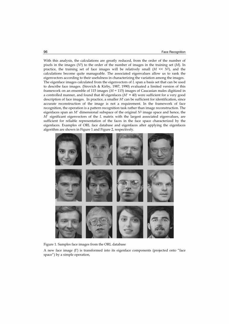
Face Recognition 96
With this analysis, the calculations are greatly reduced, from the order of the number of pixels in the images (N2) to the order of the number of images in the training set (M). In practice, the training set of face images will be relatively small (M << N2), and the calculations become quite manageable. The associated eigenvalues allow us to rank the eigenvectors according to their usefulness in characterizing the variation among the images. The eigenface images calculated from the eigenvectors of L span a basis set that can be used to describe face images. (Sirovich & Kirby, 1987, 1990) evaluated a limited version of this framework on an ensemble of 115 images (M = 115) images of Caucasian males digitized in a controlled manner, and found that 40 eigenfaces (M' = 40) were sufficient for a very good description of face images. In practice, a smaller M' can be sufficient for identification, since accurate reconstruction of the image is not a requirement. In the framework of face recognition, the operation is a pattern recognition task rather than image reconstruction. The eigenfaces span an M' dimensional subspace of the original N2 image space and hence, theM' significant eigenvectors of the L matrix with the largest associated eigenvalues, are sufficient for reliable representation of the faces in the face space characterized by the eigenfaces. Examples of ORL face database and eigenfaces after applying the eigenfaces algorithm are shown in Figure 1 and Figure 2, respectively.
Figure 1. Samples face images from the ORL database
A new face image (Γ) is transformed into its eigenface components (projected onto “face space”) by a simple operation,
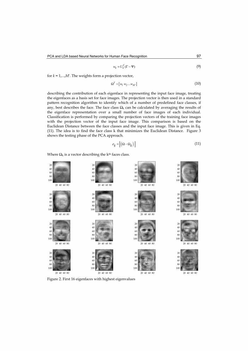
PCA and LDA based Neural Networks for Human Face Recognition 97
( )Tk kw U= Γ −Ψ (9)
for k = 1,...,M'. The weights form a projection vector,
[ ]1 2 '....TMw w wΩ = (10)
describing the contribution of each eigenface in representing the input face image, treating the eigenfaces as a basis set for face images. The projection vector is then used in a standard pattern recognition algorithm to identify which of a number of predefined face classes, if any, best describes the face. The face class Ωk can be calculated by averaging the results of the eigenface representation over a small number of face images of each individual. Classification is performed by comparing the projection vectors of the training face images with the projection vector of the input face image. This comparison is based on the Euclidean Distance between the face classes and the input face image. This is given in Eq. (11). The idea is to find the face class k that minimizes the Euclidean Distance. Figure 3 shows the testing phase of the PCA approach.
( )k kε = Ω −Ω (11)
Where Ωk is a vector describing the kth faces class.
20 40 60 80
20406080
100
20 40 60 80
20406080
100
20 40 60 80
20406080
100
20 40 60 80
20406080
100
20 40 60 80
20406080
100
20 40 60 80
20406080
100
20 40 60 80
20406080
100
20 40 60 80
20406080
100
20 40 60 80
20406080
100
20 40 60 80
20406080
100
20 40 60 80
20406080
100
20 40 60 80
20406080
100
20 40 60 80
20406080
100
20 40 60 80
20406080
100
20 40 60 80
20406080
100
20 40 60 80
20406080
100
Figure 2. First 16 eigenfaces with highest eigenvalues
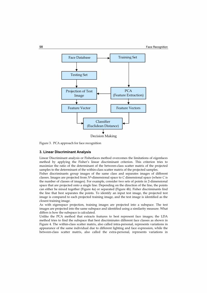
Face Recognition 98
Figure 3. PCA approach for face recognition
3. Linear Discriminant Analysis
Linear Discriminant analysis or Fisherfaces method overcomes the limitations of eigenfaces method by applying the Fisher’s linear discriminant criterion. This criterion tries to maximize the ratio of the determinant of the between-class scatter matrix of the projected samples to the determinant of the within-class scatter matrix of the projected samples. Fisher discriminants group images of the same class and separates images of different classes. Images are projected from N2-dimensional space to C dimensional space (where C is the number of classes of images). For example, consider two sets of points in 2-dimensional space that are projected onto a single line. Depending on the direction of the line, the points can either be mixed together (Figure 4a) or separated (Figure 4b). Fisher discriminants find the line that best separates the points. To identify an input test image, the projected test image is compared to each projected training image, and the test image is identified as the closest training image. As with eigenspace projection, training images are projected into a subspace. The test images are projected into the same subspace and identified using a similarity measure. What differs is how the subspace is calculated. Unlike the PCA method that extracts features to best represent face images; the LDA method tries to find the subspace that best discriminates different face classes as shown in Figure 4. The within-class scatter matrix, also called intra-personal, represents variations in appearance of the same individual due to different lighting and face expression, while the between-class scatter matrix, also called the extra-personal, represents variations in
Face Database
Testing Set
Projection of Test Image
Training Set
Feature Vector
PCA(Feature Extraction)
Feature Vectors
Classifier (Euclidean Distance)
Decision Making

PCA and LDA based Neural Networks for Human Face Recognition 99
appearance due to a difference in identity. By applying this method, we find the projection directions that on one hand maximize the distance between the face images of different classes on the other hand minimize the distance between the face images of the same class. In another words, maximizing the between-class scatter matrix Sb, while minimizing the within-class scatter matrix Sw in the projective subspace. Figure 5 shows good and bad class separation.
Figure 4. (a) Points mixed when projected onto a line. (b) Points separated when projected onto another line
Figure 5. (a) Good class separation. (b) Bad class separation
The within-class scatter matrix Sw and the between-class scatter matrix Sb are defined as
1 1
( )( )
N jCj j T
w i j i jj i
S μ μ= =
= Γ − Γ − (12)
Where Γij is the ith sample of class j, μj is the mean of class j, C is the number of classes, Nj is
the number of samples in class j.
1
( )( )C T
b j jj
S μ μ μ μ=
= − − (13)
(a)
between between
within within
(b)
(b)(a)
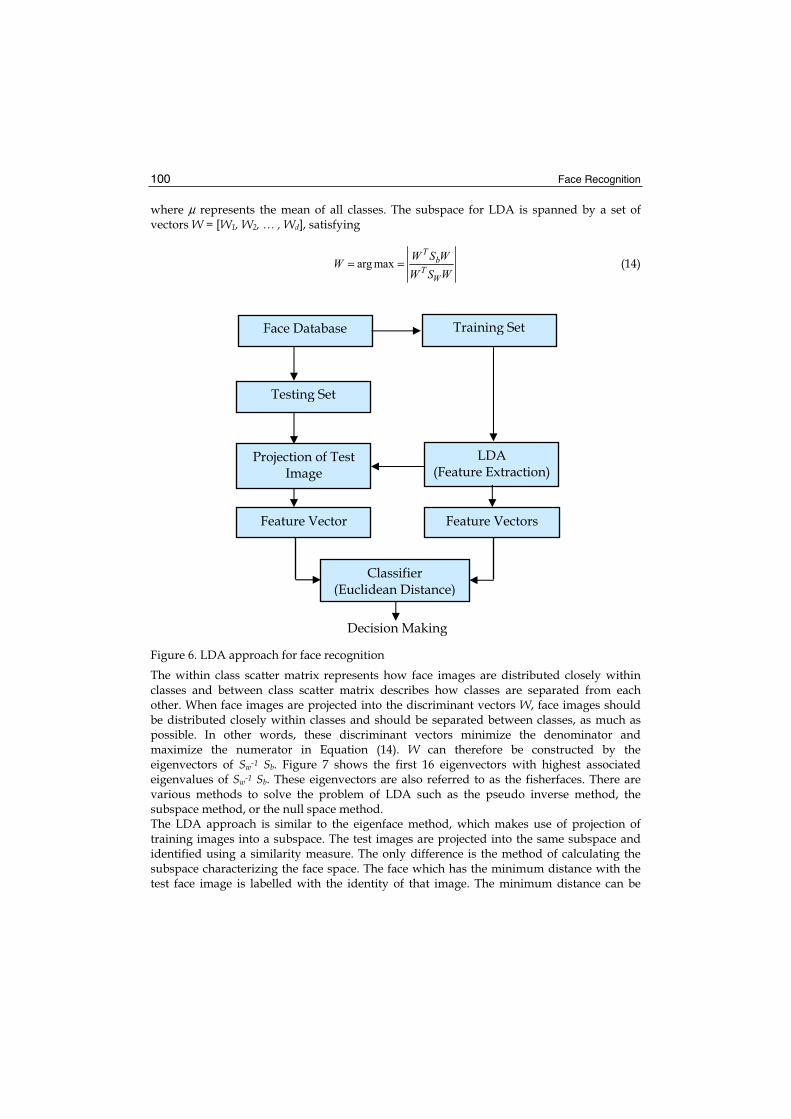
Face Recognition 100
where μ represents the mean of all classes. The subspace for LDA is spanned by a set of vectors W = [W1, W2, … , Wd], satisfying
arg maxTb
TW
W S WWW S W
= = (14)
Figure 6. LDA approach for face recognition
The within class scatter matrix represents how face images are distributed closely within classes and between class scatter matrix describes how classes are separated from each other. When face images are projected into the discriminant vectors W, face images should be distributed closely within classes and should be separated between classes, as much as possible. In other words, these discriminant vectors minimize the denominator and maximize the numerator in Equation (14). W can therefore be constructed by the eigenvectors of Sw-1 Sb. Figure 7 shows the first 16 eigenvectors with highest associated eigenvalues of Sw-1 Sb. These eigenvectors are also referred to as the fisherfaces. There are various methods to solve the problem of LDA such as the pseudo inverse method, the subspace method, or the null space method. The LDA approach is similar to the eigenface method, which makes use of projection of training images into a subspace. The test images are projected into the same subspace and identified using a similarity measure. The only difference is the method of calculating the subspace characterizing the face space. The face which has the minimum distance with the test face image is labelled with the identity of that image. The minimum distance can be
Face Database
Testing Set
Projection of Test Image
Training Set
Feature Vector
LDA(Feature Extraction)
Feature Vectors
Classifier (Euclidean Distance)
Decision Making

PCA and LDA based Neural Networks for Human Face Recognition 101
calculated using the Euclidian distance method as given earlier in Equation (11). Figure 6 shows the testing phase of the LDA approach.
20 40 60 80
20406080
100
20 40 60 80
20406080
100
20 40 60 80
20406080
100
20 40 60 80
20406080
100
20 40 60 80
20406080
100
20 40 60 80
20406080
100
20 40 60 80
20406080
100
20 40 60 80
20406080
100
20 40 60 80
20406080
100
20 40 60 80
20406080
100
20 40 60 80
20406080
100
20 40 60 80
20406080
100
20 40 60 80
20406080
100
20 40 60 80
20406080
100
20 40 60 80
20406080
100
20 40 60 80
20406080
100
Figure 7. First 16 Fisherfaces with highest eigenvalues
4. Neural Networks
Neural networks, with massive parallelism in its structure and high computation rates, provide a great alternative to other conventional classifiers and decision making systems. Neural networks are powerful tools that can be trained to perform a complex and various functions in computer vision applications, such as preprocessing (boundary extraction, image restoration, image filtering), feature extraction (extract transformed domain features), associative memory (storing and retrieving information), and pattern recognition.
4.1 Feedforward Neural Networks (FFNN)
FFNN is suitable structure for nonlinear separable input data. In FFNN model the neurons are organized in the form of layers. The neurons in a layer get input from the previous layer and feed their output to the next layer. In this type of networks connections to the neurons in the same or previous layers are not permitted. Figure 8 shows the architecture of the system for face classification.
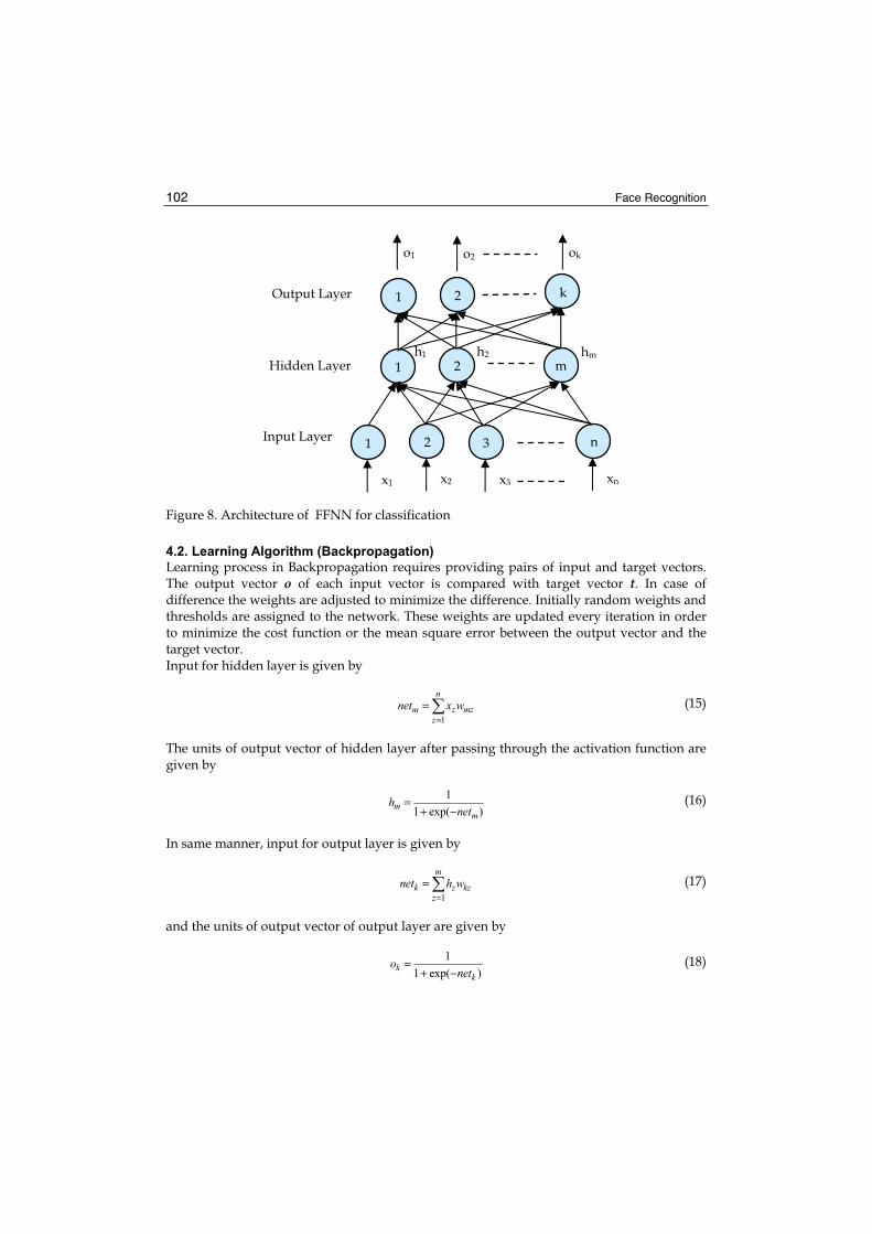
Face Recognition 102
Figure 8. Architecture of FFNN for classification
4.2. Learning Algorithm (Backpropagation)
Learning process in Backpropagation requires providing pairs of input and target vectors. The output vector o of each input vector is compared with target vector t. In case of difference the weights are adjusted to minimize the difference. Initially random weights and thresholds are assigned to the network. These weights are updated every iteration in order to minimize the cost function or the mean square error between the output vector and the target vector.Input for hidden layer is given by
1
n
m z mzz
net x w=
= (15)
The units of output vector of hidden layer after passing through the activation function are given by
1
1 exp( )m
mh
net=
+ − (16)
In same manner, input for output layer is given by
1
m
k z kzz
net h w=
= (17)
and the units of output vector of output layer are given by
1
1 exp( )k
ko
net=
+ − (18)
Output Layer
Hidden Layer
Input Layer 1
x1
2
x2
3
x3
n
xn
1 2 mhmh2h1
1 2 k
o1 o2 ok

PCA and LDA based Neural Networks for Human Face Recognition 103
For updating the weights, we need to calculate the error. This can be done by
2
1
1( )
2
k
i ii
E o t=
= − (19)
If the error is minimum than a predefined limit, training process will stop; otherwise weights need to be updated. For weights between hidden layer and output layer, the change in weights is given by
ij i jw hαδΔ = (20)
where α is a training rate coefficient that is restricted to the range [0.01,1.0], hj is the output of neuron j in the hidden layer, and δi can be obtained by
( ) (1 )i i i i it o o oδ = − − (21)
oi and ti represents the real output and target output at neuron i in the output layer respectively.Similarly, the change of the weights between hidden layer and output layer, is given by
ij Hi jw xβδΔ = (22)
where β is a training rate coefficient that is restricted to the range [0.01,1.0], xj is the output of neuron j in the input layer, and δHi can be obtained by
1
(1 )k
Hi i i j ijj
x x wδ δ=
= − (23)
xi is the output at neuron i in the input layer, and summation term represents the weighted sum of all δj values corresponding to neurons in output layer that obtained in equation (21). After calculating the weight change in all layers, the weights can simply updated by
( ) ( )ij ij ijw new w old w= + Δ (24)
5. Performance Analysis and Discussions
5.1. Training and Testing of Neural Networks
Two neural networks, one for PCA based classification and the other for LDA based classification are prepared. ORL face database is used for training and testing. The training is performed by n poses from each subject and the performance testing is performed by 10-nposes of the same subjects. After calculating the eigenfaces using PCA the projection vectors are calculated for the training set and then used to train the neural network. This architecture is called PCA-NN. Similarly, after calculation of the fisherfaces using the LDA, projection vectors are calculated for the training set. Therefore, the second neural network is trained by these vectors. This architecture is called LDA-NN (Eleyan & Demirel, 2005, 2006). Figure 9 shows the schematic diagram for the neural network training phase.
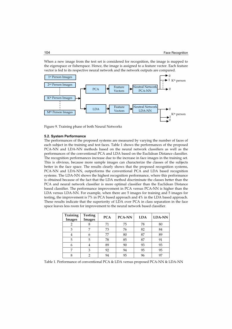
Face Recognition 104
When a new image from the test set is considered for recognition, the image is mapped to the eigenspace or fisherspace. Hence, the image is assigned to a feature vector. Each feature vector is fed to its respective neural network and the network outputs are compared.
Figure 9. Training phase of both Neural Networks
5.2. System Performance
The performances of the proposed systems are measured by varying the number of faces of each subject in the training and test faces. Table 1 shows the performances of the proposed PCA-NN and LDA-NN methods based on the neural network classifiers as well as the performances of the conventional PCA and LDA based on the Euclidean Distance classifier. The recognition performances increase due to the increase in face images in the training set. This is obvious, because more sample images can characterize the classes of the subjects better in the face space. The results clearly shows that the proposed recognition systems, PCA-NN and LDA-NN, outperforms the conventional PCA and LDA based recognition systems. The LDA-NN shows the highest recognition performance, where this performance is obtained because of the fact that the LDA method discriminate the classes better than the PCA and neural network classifier is more optimal classifier than the Euclidean Distance based classifier. The performance improvement in PCA versus PCA-NN is higher than the LDA versus LDA-NN. For example, when there are 5 images for training and 5 images for testing, the improvement is 7% in PCA based approach and 4% in the LDA based approach. These results indicate that the superiority of LDA over PCA in class separation in the face space leaves less room for improvement to the neural network based classifier.
TrainingImages
TestingImages PCA PCA-NN LDA LDA-NN
2 8 71 75 78 80 3 7 73 76 82 84 4 6 77 80 87 89 5 5 78 85 87 91 6 4 89 90 93 93 7 3 92 94 95 95 8 2 94 95 96 97
Table 1. Performance of conventional PCA & LDA versus proposed PCA-NN & LDA-NN
1st Person Images
2nd Person Images
Kth Person Images
Mth Person Images
PCA FeatureVectors
Neutral Network PCA-NN
LDAFeatureVectors
Neutral Network LDA-NN
01
0
Kth person
Kth person1
0
0

PCA and LDA based Neural Networks for Human Face Recognition 105
6. Conclusions
In this chapter, two face recognition systems, the first system based on the PCA preprocessing followed by a FFNN based classifier (PCA-NN) and the second one based on the LDA preprocessing followed by another FFNN (LDA-NN) based classifier, are introduced. The feature projection vectors obtained through the PCA and LDA methods are used as the input vectors for the training and testing of both FFNN architectures. The proposed systems show improvement on the recognition rates over the conventional LDA and PCA face recognition systems that use Euclidean Distance based classifier. Additionally, the recognition performance of LDA-NN is higher than the PCA-NN among the proposed systems.
2 3 4 5 6 7 8
70
75
80
85
90
95
100
Number of Training Faces
Recognitio
n R
ate
PCA
PCA-NN
LDA
LDA-NN
Figure 10. Recognition rate vs. number of training faces
7. References
Belhumeur, P.; Hespanha, J. & Kriegman, D. (1997). Eigenfaces vs. Fisherfaces: Recognition Using Class Specific Linear Projection. IEEE Transactions on Pattern Analysis and Machine Intelligence, Vol. 19, No. 7, (July 1997) 711-720, 0162-8828
Brunelli, R. & Poggio, T. (1993). Face recognition: Features versus Templates. IEEE Transactions on Pattern Analysis and Machine Intelligence, Vol. 15 No. 10, (Octuber 1993) 1042-1052, 0162-8828
Eleyan, A. & Demirel, H. (2005). Face Recognition System based on PCA and Feedforward Neural Networks, Proceedings of Computational Intelligence and Bioinspired Systems,pp. 935-942, 978-3-540-26208-4, Spain, June 2005, Springer-Verlag, Barcelona

Face Recognition 106
Eleyan, A. & Demirel, H. (2006). PCA and LDA Based Face Recognition Using Feedforward Neural Network Classifier, Proceedings of Multimedia Content Representation, Classification and Security, pp. 199-206, 978-3-540-39392-4, Turkey, September 2006, Springer-Verlag, Istanbul
Haykin, S. (1999). Neural Networks: A comprehensive foundation, Prentice Hall, 0-13-273350-1, New Jersey
Kirby, M. & Sirovich, L. (1990). Application of the Karhunen-Loeve Procedure for the Characterization of Human Faces, IEEE Transactions on Pattern Analysis and Machine Intelligence, Vol. 12 No. 1, (January 1990) 103-108, 0162-8828
Moghaddam, B. and Pentland, A. (1997). Probabilistic visual learning for object recognition,IEEE Transactions on Pattern Analysis and Machine Intelligence, Vol. 19 No. 7, (July 1997) 696-710, 0162-8828
Papoulis, A. & Pillai, U. (2002). Probability, random variables, and Stochastic Processes, McGraw-Hill, 0073660116, New York
Pentland, A.; Moghaddam, B. & Starner, T. (1994). Viewbased and modular eigenspaces for face recognition, In Proceedings of Computer Vision and Pattern Recognition, pp. 84–91, 0-8186-5825-8, USA, June 1994. IEEE Computer Society, Seattle
Sirovich, L. & Kirby, M. (1987). Low-Dimensional Procedure for the Characterization of Human Faces, Journal of the Optical Society of America A, Vol. 4(3), (March 1987), 519-524, 1084-7529
Turk, M. & Pentland, A. (1991). Eigenfaces for Recognition, Journal of Cognitive Neuroscience,Vol. 3, (1991) 71-86. 0898-929X
Wiskott, L.; Fellous, J. Krüger, N. & Malsburg, V. (1997). Face Recognition by Elastic Brunch Graph Matching. IEEE Transactions on Pattern Analysis and Machine Intelligence, Vol. 19 No. 7, (July 1997) 775-779, 0162-8828
Zhao, W.; Chellappa, R. & Nandhakumarm, N. (1998). Empirical performance analysis of linear discriminant classfiers. In Proceedings of Computer Vision and Pattern Recognition, pp. 164–169, 0-8186-5825-8, Canada, June 1998. IEEE Computer Society, Santa Barbara

7
Multi-View Face Recognition with Min-Max Modular Support Vector Machines
Zhi-Gang Fan and Bao-Liang Lu1
Department of Computer Science and Engineering, Shanghai Jiao Tong University Shanghai
China
1. Introduction
As a result of statistical learning theory, support vector machines (SVMs)[23] are effective classifiers for the classification problems. SVMs have been successfully applied to various pattern classification problems, such as handwritten digit recognition, text categorization and face detection, due to their powerful learning ability and good generalization ability. However, SVMs require to solve a quadratic optimization problem and need training time that are at least quadratic to the number of training samples. Therefore, many large-scale problems by using traditional SVMs are too hard to be solved. To overcome this difficulty, Lu and colleagues have proposed a min-max modular support vector machine (M3-SVM) and part-versus-part task decomposition method [16]. A very important advantage of M3-SVMs over traditional SVMs is that a two-class problem can be further decomposed into a series of two-class subproblems. The M3-network model [15] has been applied successfully to many real-world applications such as part-of-speech tagging [17], single-trial EEG signal classification [18], prediction of protein subcellular multi-locations [26], face recognition [2, 13] and text categorization [14]. The basic idea behind M3-network is the “divide and conquer” strategy. The task decomposition scheme of M3-network is based on class relations, and the instances in the same class can be further decomposed randomly [15], according to parallel hyperplanes [24], or prior knowledge [13]. The learning procedure of each subproblems is independent, and therefore parallel learning can be implemented easily. The combination strategy follows two principles, the minimization principle and the maximization principle [15]. We explore the use of M3-SVMs in multi-view face recognition. Multi-view face recognition is a more challenging task than frontal view face recognition. Face recognition techniques have been developed over the past few decades. But many of those existing face recognition techniques, such as Eigenfaces and Fisher-faces [22, 1], are only effective for frontal view faces. The difficulties of multi-view face recognition is obvious because of the complicated nonlinear manifolds existing in the data space. Using M3-SVMs, we can decompose the 1 To whom correspondence should be addressed. This work was supported in part by the National Natural Science Foundation of China under the grants NSFC 60375022 and NSFC 60473040, and The Microsoft Laboratory for Intelligent Computing and Intelligent Systems of Shanghai Jiao Tong University.

Face Recognition 108
whole complicated problem of multi-view face recognition into several relatively simpler two-class sub-problems. Every individual two-class sub-problem becomes less complicated than the original problem and it can be solved effectively. In addition, we use a SVM based discriminative feature selection (SVM-DFS) method [3] for feature selection in multi-view face recognition.
2. Part-Versus-Part Task Decomposition
For human beings, the only way to solve a complex problem is to divide it into smaller, more manageable subproblems. Breaking up a problem helps human beings deal with complex issues involved in its solution [18]. This “divide-and- conquer” strategy is also helpful to neural networks and machine learning approaches for dealing with complex learning problems. Our goal in this Section is to introduce a part-versus-part task decomposition method for training multi-class SVMs. Let be the given training data set for a K-class classification problem,
(1)
where is the input vector, is the set of training inputs, is the desired output, is the set of desired outputs, and L is the total number of training data. We have suggested that a K-class problem defined by (1) can be divided into K(K–1) = 2two-class subproblems [15], each of which is given by
(2)
where and are the training inputs belonging to class i and class j,respectively, i is the set of training inputs belonging to class i, Li denotes the number of
data in and .In this Chapter, the training data in a two-class subproblem are called positive training data if their desired outputs are +1. Otherwise, they are called negative training data. The two-class subproblems defined by (2) are called pair-wise classification in the machine learning literature [5,11]. We would like to emphasize that decomposition of a K-class problem into K(K–1) /2 two-class subproblems defined by (2) is unique for a given training data set because of the uniqueness of for i=1,...,K.Although the two-class subproblems defined by (2) are smaller than the original K-classproblem, this partition may not be adequate for parallel computation and fast learning. To speed up learning, all the large and imbalanced two-class subproblems should be further divided into relatively smaller and more balanced two-class subproblems. Assume that i is partitioned into Ni subsets in the form
(3)
where 1 Ni Li and .
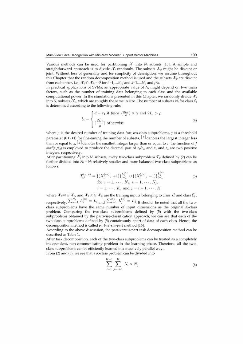
Multi-View Face Recognition with Min-Max Modular Support Vector Machines 109
Various methods can be used for partitioning i into Ni subsets [15]. A simple and straightforward approach is to divide i randomly. The subsets ij might be disjoint or joint. Without loss of generality and for simplicity of description, we assume throughout this Chapter that the random decomposition method is used and the subsets ij are disjoint from each other, i.e., ij ik = for i =1,...,K, j and k=1,...,Ni, and j k.In practical applications of SVMs, an appropriate value of Ni might depend on two main factors, such as the number of training data belonging to each class and the available computational power. In the simulations presented in this Chapter, we randomly divide i
into Ni subsets ij, which are roughly the same in size. The number of subsets Ni for class i
is determined according to the following rule:
(4)
where is the desired number of training data fort wo-class subproblems, is a threshold parameter (0< <1) for fine-tuning the number of subsets, denotes the largest integer less than or equal to z, denotes the smallest integer larger than or equal to z, the function of fmod(z1/z2) is employed to produce the decimal part of z1/z2, and z1 and z2 are two positive integers, respectively. After partitioning i into Ni subsets, every two-class subproblem ij defined by (2) can be further divided into Ni × Nj relatively smaller and more balanced two-class subproblems as follows:
(5)
where l (iu) iu and l (jv) jv are the training inputs belonging to class i and class j ,
respectively, and . It should be noted that all the two-class subproblems have the same number of input dimensions as the original K-class problem. Comparing the two-class subproblems defined by (5) with the two-class subproblems obtained by the pairwise-classification approach, we can see that each of the two-class subproblems defined by (5) containsonly apart of data of each class. Hence, the decomposition method is called part-versus-part method [16]. According to the above discussion, the part-versus-part task decomposition method can be described as Table 1. After task decomposition, each of the two-class subproblems can be treated as a completely independent, non-communicating problem in the learning phase. Therefore, all the two-class subproblems can be e ciently learned in a massively parallel way. From (2) and (5), we see that a K-class problem can be divided into
(6)

Face Recognition 110
two-class subproblems. The number of training data for each of the two-class subproblems is about
(7)
Since is independent of the number of classes K, the size of each of the two-class subproblems is much smaller than the original K-class problem for reasonable Ni
and Nj.
Step 1: Set the values of and .Step 2: Divide a K-class problem into two-class subproblems ij using (2). Step 3: If the sizes of all Tij are less than , then stop the procedure here. Otherwise, continue
with the following steps. Step 4: Determine the number of training input subsets Ni for i=1,...,K using (4).Step 5: Divide the training input set i into Ni subsets ij using (3). Step 6: Divide the two-class subproblem ij into Ni × Nj relatively smaller and simpler two
class subproblems using (5).
Table 1. The part-versus-part task decomposition method
3. Min-Max Modular Support Vector Machine
Before using M3-SVMs, for a K-class problem, we should divide the K-class problem into K(K 1)/2 two-class sub-problems according to one-against-one strategy or divide a K-class problem into K two-class subproblems according to one-against-all strategy. In this work, we use one-against-one strategy. The work procedure of M3-SVMs consists of three steps: task decomposition, SVMs training and module combination. First, every two-class problem is decomposed into relatively smaller two-class problems. Then, every smaller two-class SVM is trained. At last, all of the modules are integrated into a M3-SVM to obtain the finalsolutions to the original problem.
3.1 Support Vector Machine
Support vector machine is a machine learning technique that is well-founded in statistical learning theory. The SVM algorithm formulates the training problem as a problem that finds, among all possible separating hyperplanes, one hyperplane that maximizes the distance between the closest elements of the two classes. In practice, this is determined through solving a quadratic programming problem. SVMs have a general form of decision function for an input x as:
(8)
where i are Lagrange parameters obtained in the optimization step, yi are class labels, and K(·,·) is the kernel function. The kernel function can be various types. The linear kernel function is K(x,y)=x·y; the radial-basis function kernel function is
and the polynomial kernel function is K(x,y)=(x·y+1)n .

Multi-View Face Recognition with Min-Max Modular Support Vector Machines 111
3.2 Module Combination
After training, all the individual SVMs are integrated into aM3-SVM with the MIN unit and the MAX unit according to the following two combination principles: the minimization principle and the maximization principle [15,16]. Minimization Principle: Suppose a two-classproblem were divided into P relatively smallert wo-class subproblems, i for i=1,...,P, and also suppose that all the two-class subproblems have the same positive training data and di erent negative training data. If the P two-class subproblems are learned by the corresponding P individual SVMs, Mi for i=1,...,P, then the combination of the P trained SVMs with a MIN unit will produce the correct output for all the training inputs in , where the function of the MIN unit is to find a minimum value from its multiple inputs. The transfer function of the MIN unit is given by
(9)
where x denotes the input variable. Maximization Principle: Suppose a two-classproblem were divided into P relatively smaller two-class subproblems, i for i=1,...,P, and also suppose that all the two-class subproblems have the same negative training data and di erent positive training data. If the P two-class subproblems are learned by the corresponding P individua lSVMs, Mi for i=1,...,P, then the combination of the P trained SVMs with a MAX unit will produce the correct output for all the training input in , where the function of the MAX unit is to find a maximum value from its multiple inputs. The transfer function of the MAX unit is given by
(10)
For example, a two-class problems defined by (2) is further divided into N+ ×N relatively smaller two-class subproblems. After learning all of these two-class subproblems with SVMs, the trained N+ × N individual SVM modules are integrated into a M3-SVM with N+MIN units and one MAX unit as follows:
(11)
and
(12)
where denotes the transfer function of the trained SVM corresponding to the two-
class subproblem , and denotes the transfer function of a combination of NSVMs integrated by the MIN unit. Figure 1 illustrates the structure of a M3-SVM. Suppose that a 1-out-of-K scheme were used for output representation. Let Y denote the actual output vector of the M3-SVM for a K-class classification problem, and let denote the transfer function of the entire M3-SVM. We may then write
(13)

Face Recognition 112
According to the minimization and maximization principles, the SVMs, Mij (x) for i=1,...,K and j=i+1,...,K, and the corresponding inversions Mrs(x) for r=2,...,K and s=1,...,r
1, are integrated as
(14)
where i (x) for i=1,...,K denotes the discriminant function, which discriminates the patterns of class i from those of th eremaining classes, and the term denotes the inversion of Mri (x). It is easy to implement with Mri (x) and an INV unit. The function of the INV unit is to invert its single input; the transfer function of the INV unit is given by
(15)
where , , p ,and q are the upper and lower limits of input value input, and output, respectively. For example, and are set to +1 and -1, respectively, for support vector classifiers in the simulations below.
Figure 1. Structure of a M3-SVM consisting of N+ × N individual SVMs, N+ MIN units, and one MAX unit
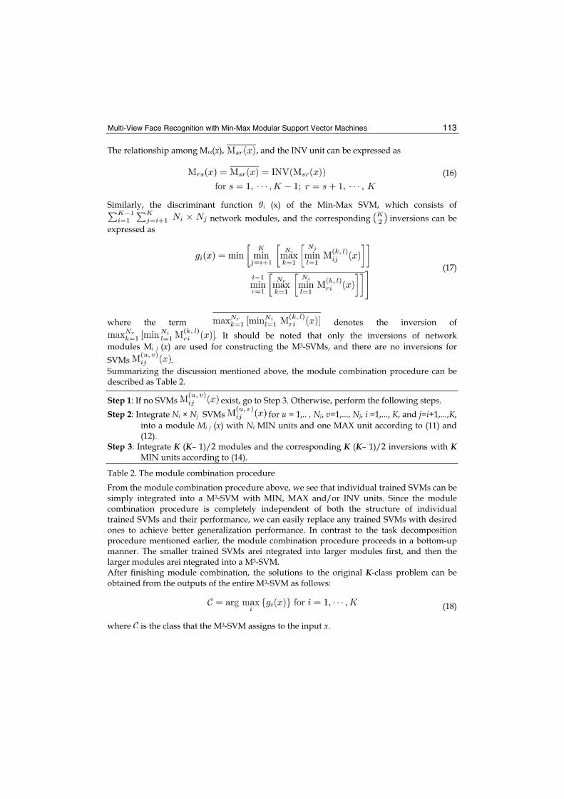
Multi-View Face Recognition with Min-Max Modular Support Vector Machines 113
The relationship among Mrs(x), , and the INV unit can be expressed as
(16)
Similarly, the discriminant function i (x) of the Min-Max SVM, which consists of network modules, and the corresponding inversions can be
expressed as
(17)
where the term denotes the inversion of . It should be noted that only the inversions of network
modules Mi j (x) are used for constructing the M3-SVMs, and there are no inversions for SVMs .Summarizing the discussion mentioned above, the module combination procedure can be described as Table 2.
Step 1: If no SVMs exist, go to Step 3. Otherwise, perform the following steps. Step 2: Integrate Ni × Nj SVMs for u = 1,.. , Ni, v=1,..., Nj, i =1,..., K, and j=i+1,...,K,
into a module Mi j (x) with Ni MIN units and one MAX unit according to (11) and (12).
Step 3: Integrate K (K– 1)/2 modules and the corresponding K (K– 1)/2 inversions with KMIN units according to (14).
Table 2. The module combination procedure
From the module combination procedure above, we see that individual trained SVMs can be simply integrated into a M3-SVM with MIN, MAX and/or INV units. Since the module combination procedure is completely independent of both the structure of individual trained SVMs and their performance, we can easily replace any trained SVMs with desired ones to achieve better generalization performance. In contrast to the task decomposition procedure mentioned earlier, the module combination procedure proceeds in a bottom-up manner. The smaller trained SVMs arei ntegrated into larger modules first, and then the larger modules arei ntegrated into a M3-SVM. After finishing module combination, the solutions to the original K-class problem can be obtained from the outputs of the entire M3-SVM as follows:
(18)
where is the class that the M3-SVM assigns to the input x.
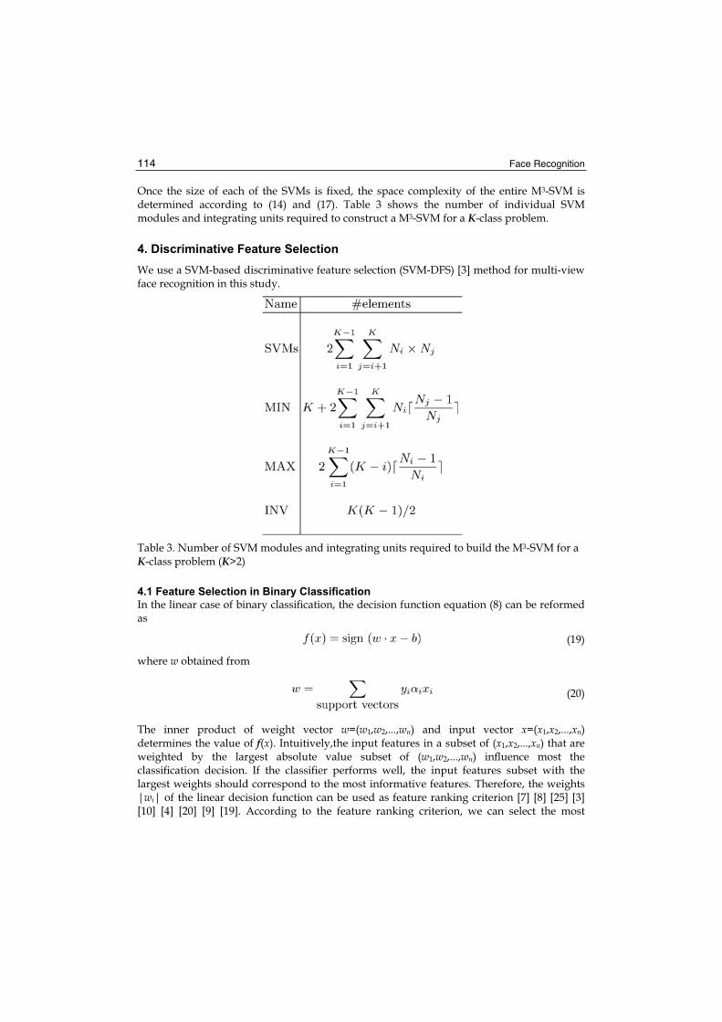
Face Recognition 114
Once the size of each of the SVMs is fixed, the space complexity of the entire M3-SVM is determined according to (14) and (17). Table 3 shows the number of individual SVM modules and integrating units required to construct a M3-SVM for a K-class problem.
4. Discriminative Feature Selection
We use a SVM-based discriminative feature selection (SVM-DFS) [3] method for multi-view face recognition in this study.
Table 3. Number of SVM modules and integrating units required to build the M3-SVM for a K-class problem (K>2)
4.1 Feature Selection in Binary Classification
In the linear case of binary classification, the decision function equation (8) can be reformed as
(19)
where w obtained from
(20)
The inner product of weight vector w=(w1,w2,...,wn) and input vector x=(x1,x2,...,xn)determines the value of f(x). Intuitively,the input features in a subset of (x1,x2,...,xn) that are weighted by the largest absolute value subset of (w1,w2,...,wn) influence most the classification decision. If the classifier performs well, the input features subset with the largest weights should correspond to the most informative features. Therefore, the weights |wi| of the linear decision function can be used as feature ranking criterion [7] [8] [25] [3] [10] [4] [20] [9] [19]. According to the feature ranking criterion, we can select the most

Multi-View Face Recognition with Min-Max Modular Support Vector Machines 115
discriminative features for the binary classification task. However, this way for feature ranking is a greedy method and we should look for more evidences for feature selection. Support vectors can be used as evidence for feature ranking [3] [10] [4], because support vectors can be used to count for di erent distributions of the features in the training data. Assume the distance between the optimal hyperplane and the support vectors is , the optimal hyperplane can be viewed as a kind of -margin separating hyperplane which is located in the center of margin ( , ). According to [23], the set of -margin separating hyperplanes has the VC dimension h bounded by the inequality
(21)
where R is the radius of a sphere which can bound the training vectors x X. Inequality (21) points out the relationship between margin and VC dimension: a larger means a smaller VC dimension. Therefore, in order to obtain high generalization ability, we should still maintain margin large after feature selection. However, because the dimensionality of original input space has been reduced after featur eselection, the margin is usually to shrink and what we can do is trying our best to make the shrink small to some extent. Therefore, in feature selection process, we should preferentially select the features which make more contribution to maintaining the margin large. This is another evidence for feature ranking. To realize this idea, a coe cient ck is introduced,
(22)
where SV+ denotes the support vectors belong to positive samples, SV– denotes the support vectors belong to negative samples, l+ denotes the number of SV+, l–denotes the number of SV–, and xi,k denotes the kth feature of support vector i in input space Rn. The larger ck
indicates that the kth feature of input space can make more contribution to maintaining the margin large. Therefore, ck can assist |wk| for feature ranking. The solution is that, combining the two evidences, we can order the features by ranking ck |wk|.In the nonlinear case of binary classification, a cost function J is computed on training samples for feature ranking. DJ(i) denotes the change in the cost function J caused by removing a given feature or, equivalently, by bringing its weight to zero. DJ(i) can be used as feature ranking criterion. In [7], DJ(i) is computed by expanding J in Taylor series to second order. At the optimum of J, the first order term can be neglected, yielding
(23)
where the change in weight corresponds to removing feature i.For the nonlinear SVMs with the nonlinear decision function f(x), the cost function J being minimized is
(24)

Face Recognition 116
where H is the matrix with elements yh yk K (xh,xk), is Lagrange parameter vector =( 1, 2,..., n), and v is a n dimensional vector of ones [7]. To compute the change in cost
function caused by removing input component i, one leaves the ’s unchanged and one recomputes matrix H. This corresponds to computing K(xh ( i), xk ( i)), yielding matrix H( i), where the notation ( i) means that component i has been removed. Thus, the feature ranking criterion for nonlinear SVMs is
(25)
Computation of DJ(i) is a little more expensive than that in the linear case. However, the change in matrix H must be computed for support vectors only, which makes it a ordable for small numbers of support vectors. For the convenience of representation, in both linear and nonlinear cases of binary classification, we denote feature ranking criterion as ri for the ith feature in the input space Rn. In linear case of binary classification, ri is
(26)
In nonlinear case of binary classification, ri is
(27)
Using feature ranking criterion ri, we can select most discriminative features for binary classification task.
4.2 Feature Selection in Multi-class Classification
In the case of multi-class classification, we use one-versus-all method for multi-class SVMs. Multi-class classification problem is much more di cult than the binary one especially when the data are of high dimensionality and the sample size is small. The classification accuracy appears to degrade very rapidly as the number of classes increases [12]. Therefore, feature selection in multi-class classification is more challenging than that in binary case. We should be more careful when extending feature selection from binary case to multi-class case. Using the statistical relationship between feature ranking and the multiple sub-models of multi-class SVMs, we propose the SVM-DFS method for features election. One-versus-all multi-class SVMs constructs K decision functions where K is the number of classes. The jth decision function fj (x) is constructed with all of the examples in the jth class with positive labels, and all other examples with negative labels. The fj (x) is a binary classification sub-model for discriminating the jth class from the all other classes. When fj (x)has the maximum value among all the sub-models, fj (x) has determined the classification result that the jth class is true. The ri j, calculated from fj (x), denotes the feature ranking criterion of the ith feature according to the binary classification sub-model fj (x). There are sure event E and impossible event Ø in probability theory. Let j denote the event that the jth class is true. According to probability theory, events 1, 2,..., k constitute a partition of the sample space
(28)

Multi-View Face Recognition with Min-Max Modular Support Vector Machines 117
and
(29)
P ( j) is the prior probability that the jth class is true. Define a random event Si as “the ithfeature is selected as discriminative feature”. Let P(Si| j) denote the conditional probability of Si given that j occurred. When event j occur, the jth binary classification sub-model fj (x)has the maximum value among all the sub-models and it is just uniquely e ective for determining the final classification result
(30)
on the premise that the fj (x) is correct. Under the condition that the jth binary classification sub-model fj (x) is e ective, we can calculate P(Si| j) through the feature ranking criterion rij
(31)
According to the theorem on the total probability, P(Si) can be calculated through P(Si| j)and P( j)
(32)
Then, P(Si) can be used as feature ranking criterion for the whole multi-class classification problem. The solution is that we can order the features by ranking P(Si) and select the features which have larger value of P(Si). In Table 4, we present an outline of the SVM-DFS algorithm. In the algorithm, T and Mt are two user defined constants. T is the number of the iteration steps. Usually, T should not be too small. Mt is the number of the features to be selected in the t iteration step. Mt can be evaluated by retraining the SVM classifiers with the Mt
selected features. Mt should be set to such a value that the margin i of each retrained SVM sub-model fi (x) is large enough
(33)
where w(i) denotes the weight vector of sub-model fi (x).According to [23],
(34)
where j(i) denotes Lagrange parameter of sub-model fi (x). Define a coe cient L:
(35)

Face Recognition 118
• Input: Training examples
X0 = {x1, x2,...xl} T
• Initialize: Indices for selected features: s=[1,2,...n]Train the SVM classifier using samples X0
• For t=1,...,T:1. Compute the ranking criteria P(Si) according to the trained SVMs 2. Order the features by decreasing P(Si), select the top Mt features, and eliminate the
other features 3. Updates by eliminating the indices which not belong to the selected features 4. Restrict training examples to selected feature indices
X=X0(:,s)
5. Train the SVM classifier using samples X • Outputs:
The small set of critical features and the final SVM classifier
Table 4. The outline of the SVM-DFS algorithm
We can use coe cient L to evaluate Mt. Mt should be set to such a value that the value of L is small enough. After the Mt discriminative features have been selected through SVM-DFS, the SVM models have to be retrained using the training data.
5. Experiments
We use the UMIST database [6], am ulti-view face database consisting of 575 gray-scale images of 20 subjects. Each of the subjects covers a wide range of poses from profile to frontal views. Figure 2 depicts some sample images of a subject in the UMIST database. This is a classification problem of 20 classes. The overall database is partitioned into two subsets: the training set and test set. The training set is composed of 240 images of 20 persons: 12 images per person are carefully chosen according to face poses. The remaining 335 images are used to form the test set. All input images are of size 112×92. We have used SVM-DFS discriminative feature selection method to reduce the dimensionality of feature space. All of the experiments were performed on a 3.0 GHz Pentium 4 PC with 1.0 GB RAM. After nonlinear dimensionality reduction [21], the distribution of face poses is shown in Figgure 3. From Figgure 3, we can see that the distribution of faces varies based on face poses. Following the observation from Figgure 3, we partition the set of training inputs for each class into four subsets by using the part-versus-part task decomposition strategy. As a result, the original 20-class classification problem has been decomposed into 3040 two-class subproblems. First, the origial 20-class classification problem has been decomposed into (20*(20-1))/2=190 two-class subproblems. Second, each two-class subproblem has been decomposed to 4*4=16 two-class subproblems. Therefore, the original problem has been decomposed into (20*(20-1))/2*4*4=3040 two-class subproblems. Every individual subproblem becomes less complicated than the original problem and it can be solved more effectively.
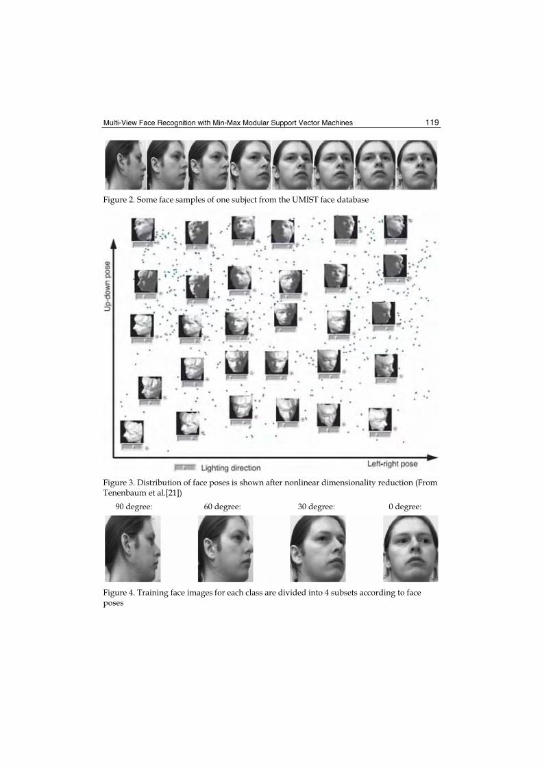
Multi-View Face Recognition with Min-Max Modular Support Vector Machines 119
Figure 2. Some face samples of one subject from the UMIST face database
Figure 3. Distribution of face poses is shown after nonlinear dimensionality reduction (From Tenenbaum et al.[21])
90 degree: 60 degree: 30 degree: 0 degree:
Figure 4. Training face images for each class are divided into 4 subsets according to face poses

Face Recognition 120
Training time (s) Methods No.
features Parallel Serial
Testtime (s)
Correct rate (%)
SVMs (rbf kernel)
300
200
150
100
30
25
25
20
0.862
0.748
0.703
0.685
13.588
12.654
11.865
11.269
1.522
0.976
0.757
0.478
92.8358
92.2388
90.1493
82.3881
M3-SVMs(rbfkernel)
300
200
150
100
20
15
10
10
0.531
0.447
0.386
0.359
15.273
13.413
12.587
12.165
1.647
1.215
0.873
0.526
93.1343
92.5373
91.3433
83.8806
Table 5. Test results on UMIST face database
To evaluate the e ectiveness of the proposed method, the multi-view face recognition problem was learned by both M3-SVMs and standard SVMs. The one-versus-all method is used for training the standard SVMs. A radial-basis function kernel for SVMs is used, the parameter C=10000, and is set to the optimal values. The experimental results are shown in Table 5. From Table 5, we can see that M3-SVMs can obtain better generalization performance than the standard SVMs when the original problem is decomposed into 3040 two-class subproblems, and meanwhile the training time can be reduced in a parallel way. The parallel training is to train all the sub-modules at the same time in parallel. And the serial training is to train all the individual modules one-by-one in serial. In parallel training way, M3-SVMs can make the training speed faster comparing to the standard SVMs. The results in Table 5 also indicate that even though in low feature space after discriminative feature selection, M3-SVMs are still more accurate than the standard SVMs.
6. Conclusions
We have applied the min-max modular support vector machine and the part-versus-part task decomposition method to dealing with multi-view face recognition problems. We have demonstrated that face pose information can be easily incorporated into the procedure of dividing a multi-view face recognition problem into a series of relatively easier two-class subproblems. We have performed some experiments on the UMIST database and compared with the standard support vector machines. The experimental results indicate that the min-max modular support vector machine can improve the accuracy of multi-view face recognition and reduce the training time. As a future work, we will perform experiments on large-scale face databases with various face poses. We believe that the min-max modular support vector machine with incorporating pose information into task decomposition will have more advantages over traditional support vector machines in both training time and recognition accuracy when a more number of training samples are available.

Multi-View Face Recognition with Min-Max Modular Support Vector Machines 121
7. References
Belhumeur, P., Hespanda, J., Kiregeman, D. Eigenfaces vs. Fisherfaces: Recognition Using Class Specific Linear Projection. IEEE Trans. Pattern Analysis and Machine Intelligence, vol. 19, no. 7, (1997) 711-720. [1]
Fan, Z. G., Lu, B. L. (2005). Multi-view Face Recognition with Min-Max Modular SVMs, Proc.ICNC '05, Lecture Notes in Computer Science, vol.3611, pp.396-399. [2]
Fan, Z. G., Lu, B. L. Fast Recognition of Multi-View Faces with Feature Selection, 10th IEEE International Conference on Computer Vision (ICCV'05), vol. 1, pp. 76-81, 2005. [3]
Fan, Z. G., Wang K. A., Lu, B. L. Feature Selection for Fast Image Classification with Support Vector Machines, Proc. ICONIP 2004 , LNCS 3316, pp. 1026-1031, 2004. [4]
Friedman, J. H., Another approach to polychotomous classification, Technical Report,(ftp://stat.stanford.edu/pub/friedman/poly.ps.Z), Stanford University, 1996. [5]
Graham, D.B., Allinson, N.M. Characterizing virtual eigensignatures for general purpose face recognition. In: Face Recognition: From Theory to Applications, NATO ASI Series F, Computer and Systems Sciences, vol. 163, (1998) 446-456. [6]
Guyon, I., Weston, J., Barnhill, S., Vapnik, V. Gene Selection for Cancer Classification using Support Vector Machines, Machine Learning, Vol. 46, pp. 389-422, 2002. [7]
Guyon, I., Elisseeff, A. An introduction to variable and feature selection, Journal of Machine Learning, Vol. 3, pp. 1157-1182, 2003. [8]
Guyon, I., Gunn, S. R., Ben-Hur, A., Dror, G. Result Analysis of the NIPS 2003 Feature Selection Challenge, NIPS 2004, 2004. [9]
Heisele, B., Serre, T., Prentice, S., Poggio, T. Hierarchical classification and feature reduction for fast face detection with support vector machine, Pattern Recognition, Vol. 36, pp. 2007-2017, 2003. [10]
Krebel, U., Pairwise classification and support vector machines, In B. SchÄolkopf, C. J. C. Burges, and A. J. Smola, editors, Advances in Kernal Methods {Support Vector Learning), pp. 255-268, Cambridge, MA, 1999, MIT Press. [11]
Li, T., Zhang, C., Ogihara, M. A comparative study of feature selection and multiclass classification methods for tissue classification based on gene expression, Bioinformatics, Vol. 20, No. 15, pp. 2429-2437, 2004. [12]
Lian, H. C., Lu, B. L., Takikawa, E, Hosoi, S. (2005). Gender Recognition Using a Min-Max Modular Support Vector Machine, Proc. ICNC'05, Lecture Notes in Computer Science,vol.3611, pp.438-441. [13]
Liu, F. Y., Wu, K., Zhao, H., Lu, B. L. (2005). Fast Text Categorization with Min-Max Modular Support Vector Machines, IJCNN '05, vol.1, pp570-575. [14]
Lu, B.L., Ito, M. Task decomposition and module combination based on class relations: a modular neural network for pattern classification. IEEE Transactions on Neural Networks, vol.10, (1999) 1244 -1256 [15]
Lu, B.L., Wang, K.A., Utiyama, M., Isahara, H. A part-versus-part method for massively parallel training of support vector machines. In: Proceedings of IJCNN '04, Budapast, July 25-29(2004) [16]
Lu, B. L., Ma, Q., Ichikawa, M., Isahara, H. (2003). E±cient Part-of-Speech Tagging with a Min-Max Modular Neural Network Model, Applied Intelligence, vol.19, pp.65-81. [17]

Face Recognition 122
Lu, B. L., Shin, J., Ichikawa, M. (2004). Massively Parallel Classification of Single-Trial EEG Signals Using a Min-Max Modular Neural Network, IEEE Trans. Biomedical Engineering, vol. 51, pp. 551-558. [18]
Mao, K. Z. Feature Subset Selection for Support Vector Machines Through Discriminative Function Pruning Analysis, IEEE Trans. Systems, Man, and Cybernetics, vol. 34, no. 1, 2004. [19]
Mladenic, D., Brank, J., Grobelnik, M., Milic-Frayling, N. Feature selection using linear classifier weights: interaction with classification models", Proceedings of the 27th annual international ACM SIGIR conference, Vol. 1, pp. 234-241, 2004. [20]
Tenenbaum, J. B., Silva, V. De, Langford, J. C., (2000). A global geometric framework for nonlinear dimensionality reduction. Science, Vol. 290, No. 5500, pp. 2319- 2323. [21]
Turk M., Pentland, A. Eigenfaces for Recognition. Journal of Cognitive Neuro-science, vol. 3, no. 1, (1991) 71-86 [22]
Vapnik, V. N. The Nature of Statistical Learning Theory. Springer-Verlag, New York (2000) [23] Wang, K. A., Zhao, H., Lu, B. L. (2005). Task Decomposition Using Geometric Relation for
Min-Max Modular SVMs, ISNN 2005, Lecture Notes in Computer Science, vol.3 496, pp. 887-892. [24]
Weston, J., Elisseeff, A., Schoelkopf, B., Tipping, M. Use of the zero norm with linear models and kernel methods, Journal of Machine Learning, Vol. 3, pp. 1439- 1461, 2003. [25]
Yang, Y., Lu, B. L. (2006). Prediction of Protein Subcellular Multi-Locations with a Min-Max Modular Support Vector Machined, in Proceedings of Third International Symposium on Neural Networks (ISNN 2006). [26]

8
Design, Implementation and Evaluation of Hardware Vision Systems dedicated
to Real-Time Face Recognition
Ginhac Dominique, Yang Fan and Paindavoine Michel LE2I - University of Burgundy
France
1. Introduction
Human face recognition is an active area of research spanning several disciplines such as image processing, pattern recognition, and computer vision. Different techniques can be used to track and process faces (Yang et al, 2001), e.g., neural networks approaches (Férand et al., 2001, Rowley et al., 1998), eigenfaces (Turk & Pentland, 1991), and the Markov chain (Slimane et al., 1999). Most researches have concentrated on the algorithms of segmentation, feature extraction, and recognition of human faces, which are generally realized by software implementation on standard computers. However, many applications of human face recognition such as human-computer interfaces, model-based video coding, and security control (Kobayashi, 2001, Yeh & Lee, 1999) need to be high-speed and real-time, for example, passing through customs quickly while ensuring security. Liu (1998) realized an automatic human face recognition system using the optical correlation technique after necessary preprocessing steps. Buhmann et al. (1994) corrected changes in lighting conditions with an analog VLSI silicon retina in order to increase the face recognition rate. Matsumoto & Zelinsky (2000) implemented in real time a head pose and gaze direction measurement system on the vision processing board Hitachi IP5000. For the last years, our laboratory has focused on face processing and obtained interesting results concerning face tracking and recognition by implementing original dedicated hardware systems. Our aim is to implement on embedded systems efficient models of unconstrained face tracking and identity verification in arbitrary scenes. The main goal of these various systems is to provide efficient robustness algorithms that only require moderated computation in order 1) to obtain high success rates of face tracking and identity verification and 2) to cope with the drastic real-time constraints. The goal of this chapter is to describe three different hardware platforms dedicated to face recognition. Each of them has been designed, implemented and evaluated in our laboratory. In a first part, we describe a real time vision system that allows the localization of faces and the verification of their identity. This embedded system is based on image processing techniques and the radial basis function (RBF) neural network approach. The robustness of this system has been evaluated quantitatively on real video sequences. We also describe three hardware implementations of our model on embedded systems based, respectively, on field programmable gate array (FPGA), zero instruction set computer (ZISC) chips, and

Face Recognition 124
digital signal processor (DSP) TMS320C62.We analyze the algorithm complexity and present results of hardware implementations in terms of resources used and processing speed. In a second part, we describe the main principles of a full-custom vision system designed in a classical 0.6 μm CMOS Process. The development of this specific vision chip is motivated by the fact that preliminary works have shown that simplified RBF networks gave interesting results but imposed a fast feature extraction to reduce the size of the input vectors of the RBF network. So, in order to unload a consequent calculation part of FPGA, we have decided to design an artificial retina embedding the extraction of input vectors of RBF network. For this purpose, a VLSI sensor is proposed to realize the image acquisition, to extract a window of interest in the whole image, to evaluate the RBF vectors as means values of consecutive pixels on lines and columns. A prototype based on this principle, has been designed, simulated and evaluated. In a third part, we describe a new promising approach based on a simple and efficient hardware platform that performs mosaicking of panoramic faces. Our objective is to study the panoramic face construction in real time. So, we built an original acquisition system composed of five standard cameras, which can take simultaneously five views of a face at different angles. Then, we chose an easily hardware-achievable algorithm, based on successive linear transformations, in order to compose a panoramic face from the five views. The method has been tested on a large number of faces. In order to validate our system, we also conducted a preliminary study on panoramic face recognition, based on the principal-component method. Experimental results show the feasibility and viability of our system. This rest of the chapter is organized as follows. Section II, III and IV describe the three systems designed by our team. In each of these sections, we present the principles of the system, the description of the hardware platform and the main simulated and experimental results. Finally, the last section presents conclusion and future works.
2. Real-time face tracking based on a RBF Neural Network
Face recognition is a very challenging research problem due to variations in illumination, facial expression and pose. It has received extensive attention during the past 20 years, not only because of the potential applications in fields such as Human Computer Interaction, biometrics and security, but also because it is a typical pattern recognition problem whose solution would help in solving other classification problems. The recognition technique used in this first embedded system is based on Radial Basis Function (RBF) networks. The RBF neural networks have been successfully applied to face recognition. Rosenblum et al. (1996) developed a system of human expressions recognition from motion based on RBF neural network architecture. Koh et al. (2002) performed an integrated automatic face detection and recognition system using the RBF networks approach. Howell & Buxton (1998) compared RBF networks with other neural network techniques on a face recognition task for applications involving identification of individuals using low-resolution video information. The RBF networks give performance errors of only 5%–9% on generalization under changes of orientation, scale, pose. Their main advantages are computational simplicity and robust generalization. Howell and Buxton showed that the RBF network provides a solution which can process test images in interframe periods on a low-cost processor. The simplicity and the robust generalization of the RBF networks approach, with its advantages due to the fact that it can be mapped directly into the existing neural networks chips lead us to elaborate our model using a RBF classifier.

Design, Implementation and Evaluation of Hardware Vision Systems dedicated to Real-Time Face Recognition 125
We chose three commercial embedded systems for hardware implementations of face tracking and identity verification. These systems are based, respectively, on most common electronic devices: FPGA, zero instruction set computer (ZISC) chips, and digital signal processor (DSP) TMS320C62. We obtained processing speeds of, respectively, for three implementations: 14 images/s, 25 images/s, and 4.8 images/s.
Figure 1. Radial basis function neural network
2.1 Description of the RBF model
The RBF neural network (Park & Sandberg, 1991) has a feedforward architecture with an input layer, a hidden layer, and an output layer as shown in Figure 1. The input layer of this network has N units for an N-dimensional input vector. The input units are fully connected to the hidden layer units, which are in turn connected to the J output layer units, where J is the number of output classes. RBF networks belong to the category of kernel networks. Each hidden node computes a kernel function on input data, and the output layer achieves a weighted summation of the kernel functions. Each node is characterized by two important associated parameters: 1), its center and 2) the width of the radial function. A hidden node provides the highest output value when the input vector is close to its center and this output value decreases as the distance from the center increases. Several distances can be used to estimate the distance from a center but the most common is the Euclidean distance d(x). The activation function of the hidden node is often a Gaussian function such that each hidden node is defined by two parameters: its center ci and the width of the radial function i.
)/)(( 22
exp)()( ixdii xfcxxd σ−=−= (1)
The training procedure undergoes a two-step decomposition: estimating ci and i and estimating the weights between the hidden layer and output layer. The estimation of these parameters is largely detailed in Yang & Paindavoine (2003).
2.2 Description and test of our model
Many face recognition algorithms require segmenting the face from the background, and subsequently extracting features such as eyes, nose, and mouth for further processing. We propose an integrated automatic face localization and identification model only using a classifier which responds to the question, “Does the input vector correspond or not the

Face Recognition 126
person to be verified?” The idea behind this is to simplify the model and reduce computation complexity in order to facilitate hardware implementations.
Figure 2. Structure of the face tracking and identity verification model
Figure 2 represents the structure of our model. The size of faces in the scene varies from 40 x 32 pixels to 135 x 108 pixels with four scales. The ratio between any two scales is fixed to 1.5 (Howel & Buxton, 1998).We first subsample the original scene and extract only the 40 x 32 windows in the 4 subsampled images. Each pre-processed 40 x 32 window is then fed to RBF network as an input vector. After the training procedure, the hidden nodes obtained are partially connected to the output layer. In fact, the hidden nodes associated with one person are only connected to the output node representing this class. This technique reduces data dependencies and is computationally more efficient (Koh et al., 2002). The decision stage yields the presence, position, identity and scale of the faces using the maximal output values of the RBF neural network. In order to evaluate and validate our model, we made experiments based on video sequences of 256 images. In all sequences, the scene size is 288 x 352 pixels and they are zero, one, two, or three different faces presented (see. Figure 4). We have decided to verify two persons in these sequences. The 12 same training faces (see Figure 3) are used in order to compare the different configurations of the model.
Figure 3. 2x12 learning faces
First, in order to simplify future hardware implementations, the first phase has consisted in reducing the input vectors length of the RBF network. In the preprocessing stage, we use first all pixels of each 40 x 32 window to compose the feature vectors. Each pixel represents one component of the vector. So, the input vectors of RBF neural network have 40 x 32 components. Second, we minimize the number of components in order to reduce the
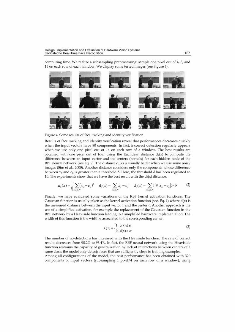
Design, Implementation and Evaluation of Hardware Vision Systems dedicated to Real-Time Face Recognition 127
computing time. We realize a subsampling preprocessing: sample one pixel out of 4, 8, and 16 on each row of each window. We display some tested images (see Figure 4).
Figure 4. Some results of face tracking and identity verification
Results of face tracking and identity verification reveal that performances decreases quickly when the input vectors have 80 components. In fact, incorrect detection regularly appears when we use only one pixel out of 16 on each row of a window. The best results are obtained with one pixel out of four using the Euclidean distance d2(x) to compute the difference between an input vector and the centers (kernels) for each hidden node of the RBF neural network (see Eq. 2). The distance d1(x) is usually better when we use some noisy images (Sim et al., 2000). Another distance considers only the components whose difference between xn and cn is greater than a threshold δ. Here, the threshold δ has been regulated to 10. The experiments show that we have the best result with the d0(x) distance.
( ) δ>−∀=−=−=≤≤≤≤≤≤
nnNnNn
nnNn
nn cxxcxxcxxd 1)(d)(d)(1
0
1
1
1
2
2 (2)
Finally, we have evaluated some variations of the RBF kernel activation functions. The Gaussian function is usually taken as the kernel activation function (see. Eq. 1) where d(x) is the measured distance between the input vector x and the center c. Another approach is the use of a simplified activation, for example the replacement of the Gaussian function in the RBF network by a Heaviside function leading to a simplified hardware implementation. The width of this function is the width associated to the corresponding center.
>≤
=σσ
d(x)0
d(x)1)(xf (3)
The number of no-detections has increased with the Heaviside function. The rate of correct results decreases from 98.2% to 93.4%. In fact, the RBF neural network using the Heaviside function restrains the capacity of generalization by lack of interactions between centers of a same class: the model only detects faces that are sufficiently close to training examples. Among all configurations of the model, the best performance has been obtained with 320 components of input vectors (subsampling 1 pixel/4 on each row of a window), using
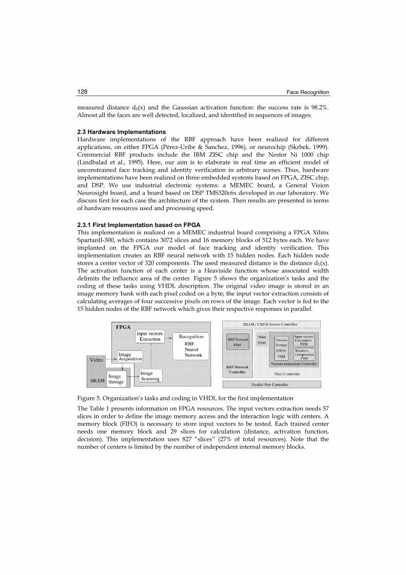
Face Recognition 128
measured distance d0(x) and the Gaussian activation function: the success rate is 98.2%. Almost all the faces are well detected, localized, and identified in sequences of images.
2.3 Hardware Implementations
Hardware implementations of the RBF approach have been realized for different applications, on either FPGA (Pérez-Uribe & Sanchez, 1996), or neurochip (Skrbek, 1999). Commercial RBF products include the IBM ZISC chip and the Nestor Ni 1000 chip (Lindbalad et al., 1995). Here, our aim is to elaborate in real time an efficient model of unconstrained face tracking and identity verification in arbitrary scenes. Thus, hardware implementations have been realized on three embedded systems based on FPGA, ZISC chip, and DSP. We use industrial electronic systems: a MEMEC board, a General Vision Neurosight board, and a board based on DSP TMS320c6x developed in our laboratory. We discuss first for each case the architecture of the system. Then results are presented in terms of hardware resources used and processing speed.
2.3.1 First Implementation based on FPGA
This implementation is realized on a MEMEC industrial board comprising a FPGA Xilinx SpartanII-300, which contains 3072 slices and 16 memory blocks of 512 bytes each. We have implanted on the FPGA our model of face tracking and identity verification. This implementation creates an RBF neural network with 15 hidden nodes. Each hidden node stores a center vector of 320 components. The used measured distance is the distance d1(x). The activation function of each center is a Heaviside function whose associated width delimits the influence area of the center. Figure 5 shows the organization’s tasks and the coding of these tasks using VHDL description. The original video image is stored in an image memory bank with each pixel coded on a byte; the input vector extraction consists of calculating averages of four successive pixels on rows of the image. Each vector is fed to the 15 hidden nodes of the RBF network which gives their respective responses in parallel.
Figure 5. Organization’s tasks and coding in VHDL for the first implementation
The Table 1 presents information on FPGA resources. The input vectors extraction needs 57 slices in order to define the image memory access and the interaction logic with centers. A memory block (FIFO) is necessary to store input vectors to be tested. Each trained center needs one memory block and 29 slices for calculation (distance, activation function, decision). This implementation uses 827 “slices” (27% of total resources). Note that the number of centers is limited by the number of independent internal memory blocks.
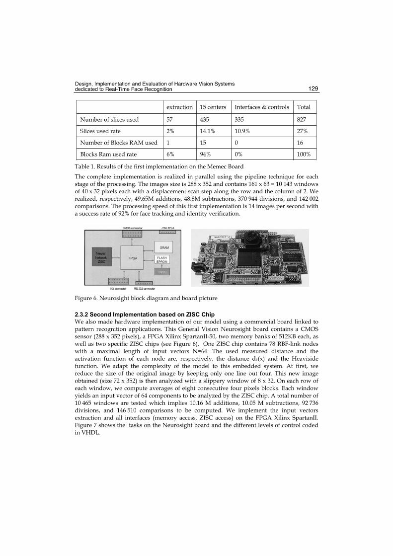
Design, Implementation and Evaluation of Hardware Vision Systems dedicated to Real-Time Face Recognition 129
extraction 15 centers Interfaces & controls Total
Number of slices used 57 435 335 827
Slices used rate 2% 14.1% 10.9% 27%
Number of Blocks RAM used 1 15 0 16
Blocks Ram used rate 6% 94% 0% 100%
Table 1. Results of the first implementation on the Memec Board
The complete implementation is realized in parallel using the pipeline technique for each stage of the processing. The images size is 288 x 352 and contains 161 x 63 = 10 143 windows of 40 x 32 pixels each with a displacement scan step along the row and the column of 2. We realized, respectively, 49.65M additions, 48.8M subtractions, 370 944 divisions, and 142 002 comparisons. The processing speed of this first implementation is 14 images per second with a success rate of 92% for face tracking and identity verification.
Figure 6. Neurosight block diagram and board picture
2.3.2 Second Implementation based on ZISC Chip
We also made hardware implementation of our model using a commercial board linked to pattern recognition applications. This General Vision Neurosight board contains a CMOS sensor (288 x 352 pixels), a FPGA Xilinx SpartanII-50, two memory banks of 512KB each, as well as two specific ZISC chips (see Figure 6). One ZISC chip contains 78 RBF-link nodes with a maximal length of input vectors N=64. The used measured distance and the activation function of each node are, respectively, the distance d1(x) and the Heaviside function. We adapt the complexity of the model to this embedded system. At first, we reduce the size of the original image by keeping only one line out four. This new image obtained (size 72 x 352) is then analyzed with a slippery window of 8 x 32. On each row of each window, we compute averages of eight consecutive four pixels blocks. Each window yields an input vector of 64 components to be analyzed by the ZISC chip. A total number of 10 465 windows are tested which implies 10.16 M additions, 10.05 M subtractions, 92 736 divisions, and 146 510 comparisons to be computed. We implement the input vectors extraction and all interfaces (memory access, ZISC access) on the FPGA Xilinx SpartanII. Figure 7 shows the tasks on the Neurosight board and the different levels of control coded in VHDL.
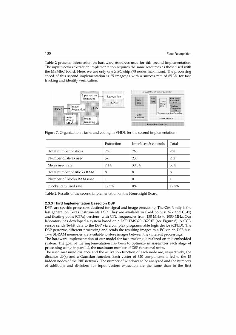
Face Recognition 130
Table 2 presents information on hardware resources used for this second implementation. The input vectors extraction implementation requires the same resources as those used with the MEMEC board. Here, we use only one ZISC chip (78 nodes maximum). The processing speed of this second implementation is 25 images/s with a success rate of 85.3% for face tracking and identity verification.
Figure 7. Organization’s tasks and coding in VHDL for the second implementation
Extraction Interfaces & controls Total
Total number of slices 768 768 768
Number of slices used 57 235 292
Slices used rate 7.4% 30.6% 38%
Total number of Blocks RAM 8 8 8
Number of Blocks RAM used 1 0 1
Blocks Ram used rate 12.5% 0% 12.5%
Table 2. Results of the second implementation on the Neurosight Board
2.3.3 Third Implementation based on DSP
DSPs are specific processors destined for signal and image processing. The C6x family is the last generation Texas Instruments DSP. They are available in fixed point (C62x and C64x) and floating point (C67x) versions, with CPU frequencies from 150 MHz to 1000 MHz. Our laboratory has developed a system based on a DSP TMS320 C6201B (see Figure 8). A CCD sensor sends 16-bit data to the DSP via a complex programmable logic device (CPLD). The DSP performs different processing and sends the resulting images to a PC via an USB bus. Two SDRAM memories are available to store images between the different processings. The hardware implementation of our model for face tracking is realized on this embedded system. The goal of the implementation has been to optimize in Assembler each stage of processing using, in parallel, the maximum number of DSP functional units. The used measured distance and the activation function of each node are, respectively, the distance d0(x) and a Gaussian function. Each vector of 320 components is fed to the 15 hidden nodes of the RBF network. The number of windows to be analyzed and the numbers of additions and divisions for input vectors extraction are the same than in the first
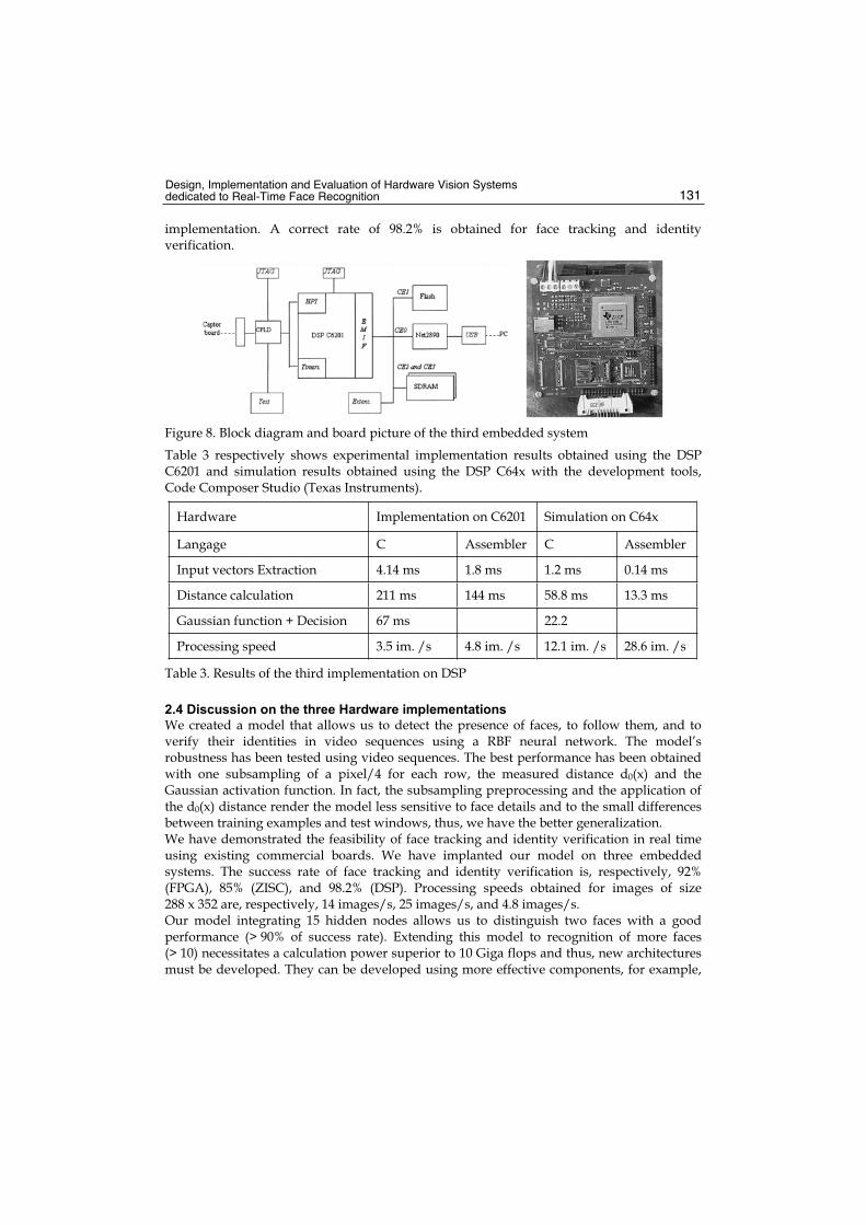
Design, Implementation and Evaluation of Hardware Vision Systems dedicated to Real-Time Face Recognition 131
implementation. A correct rate of 98.2% is obtained for face tracking and identity verification.
Figure 8. Block diagram and board picture of the third embedded system
Table 3 respectively shows experimental implementation results obtained using the DSP C6201 and simulation results obtained using the DSP C64x with the development tools, Code Composer Studio (Texas Instruments).
Hardware Implementation on C6201 Simulation on C64x
Langage C Assembler C Assembler
Input vectors Extraction 4.14 ms 1.8 ms 1.2 ms 0.14 ms
Distance calculation 211 ms 144 ms 58.8 ms 13.3 ms
Gaussian function + Decision 67 ms 22.2
Processing speed 3.5 im. /s 4.8 im. /s 12.1 im. /s 28.6 im. /s
Table 3. Results of the third implementation on DSP
2.4 Discussion on the three Hardware implementations
We created a model that allows us to detect the presence of faces, to follow them, and to verify their identities in video sequences using a RBF neural network. The model’s robustness has been tested using video sequences. The best performance has been obtained with one subsampling of a pixel/4 for each row, the measured distance d0(x) and the Gaussian activation function. In fact, the subsampling preprocessing and the application of the d0(x) distance render the model less sensitive to face details and to the small differences between training examples and test windows, thus, we have the better generalization. We have demonstrated the feasibility of face tracking and identity verification in real time using existing commercial boards. We have implanted our model on three embedded systems. The success rate of face tracking and identity verification is, respectively, 92% (FPGA), 85% (ZISC), and 98.2% (DSP). Processing speeds obtained for images of size 288 x 352 are, respectively, 14 images/s, 25 images/s, and 4.8 images/s. Our model integrating 15 hidden nodes allows us to distinguish two faces with a good performance (> 90% of success rate). Extending this model to recognition of more faces (> 10) necessitates a calculation power superior to 10 Giga flops and thus, new architectures must be developed. They can be developed using more effective components, for example,

Face Recognition 132
FPGA Virtex 5 series or DSP TMS320C64, thus allowing a very rapid processing speed and better performance of face tracking and identity verification.
3. Design of a CMOS sensor dedicated to the extraction of input vectors
A system capable of doing face localization and recognition in real time has many applications in intelligent man-machine interfaces and in other domains such as very low bandwidth video conferencing, and video e-mail. This section describes the main principles of a vision system, allowing to detect automatically the faces presence, to localize and to follow them in video sequences. The preliminary works, described in the previous section, have shown that RBF networks gave interesting results (Yang & Paindavoine, 2003) but imposed a fast feature extraction to reduce the size of the input vectors of the RBF network. So, the main goal of the current project is the development and the characterisation of a specific CMOS sensor able to realize the image acquisition, to extract a window of interest in the whole image and to evaluate means values of consecutive pixels on lines and columns. A first image sensor with electronic shutter has been integrated in a 0.6 μm digital CMOS technology. The pixel cell consists of four transistors and a photodiode. Each pixel measures 30 μm by 30 μm and has a fill factor of about 40%. Each selected pixel produces a current which is transferred to the column readout amplifiers and converted by a pipeline ADC to produce a digital output. The two analog and digital values are then multiplexed to the output of the sensor. This retina also includes a logic command in order to realize acquisition of subwindows with random size and position.
3.1 Overview of the Chip Architecture
An active pixel sensor (APS) is a detector array that has at least one active transistor within the pixel unit cell (Nakamura et al., 1997). Currently, active pixel sensor technology integrates electronic signal processing and control with smart camera function onto the same single chip as a high performance image sensor (Kemeny et al., 1997). CMOS image sensors with integrated signal processing have been implemented for a number of applications (Aw & Wooley, 1996). Most current CMOS sensors have been designed for video applications, and digital photography. Improvement continues to be made because current mode image sensors have several advantages for example, low power supply, smaller place, higher operation speed (Huang & Horsney, 2003, Tabet & Horsney, 2001). The following subsections describe the design of the image sensor using a standard 0.6 μm CMOS process. The design is based on the integration of four MOS transistors for each pixel, a column readout amplifier, a sequential control unit which includes variable input counters, decoders, multiplexers and finally an analog to digital converter. Results based on design and simulations are presented for each part of the circuit. The architecture of the proposed image sensor is shown in Figure 9. This figure first describes the core of the system represented by the m x m array of transistors active pixels. On the left, the second block, the row decoder is charged to send to each line of pixels the control signals allowing pixel resetting, shutter opening or closing, pixel readout, ... On the bottom of the circuit, the third block is made up of amplifiers, multiplexers and column decoders whose purpose is to detect, amplify and route the signal resulting from readout column to the output of the circuit. The automatic scan of the whole array of pixels or a

Design, Implementation and Evaluation of Hardware Vision Systems dedicated to Real-Time Face Recognition 133
subwindow of pixels is implemented by a sequential control unit which generates the internal signals to the row and column decoders. Finally, the analog output voltages are proportional to the grey scale intensity of the image. They are passed to an analog to digital converter (ADC) (as seen on the right of the block diagram). This ADC allows the conversion of analog values in digitals values which will be later processed by a DSP or a FPGA outside the chip.
Figure 9. Image Sensor Architecture
3.2 Design of the Active Pixel Sensor
We used a standard pixel as described in the left part of Figure 2 because it is a simple and stable design (Aw & Wooley, 1996, Coulombe et al., 2000). It consists of 3 PMOS transistors, a NMOS transistor for row access and a photodiode. m_1 is the shutter transistor, m_2 is the reset transistor, and the transistor m_3 acts as a transconductance buffer that converts the voltage at VPix into a current. The vertical column lines in the array are implemented using second-layer metal. First layer metal is used for the horizontal row lines. Third-layer metal is connected to Vss and covers all active areas of the pixel except the photodiodes.
Figure 10. Pixel circuit schematic and results of simulation
Prior to the image acquisition, m_1 and m_2 are on, resetting node VPhoto and VPix to the VReset
value. After reset, when m_1 is on and m_2 turned off, the charges generated by absorption of light are integrated onto the parasitic capacitances of the photodiode and the transistor

Face Recognition 134
m_3. So, during the exposure period, voltage is accumulated at node VPhoto and Vpix. At the end of the exposure period, the shutter is closed by turning off m_1. Consequently, the photosignal is stored as a voltage on node Vpix. Finally, during readout, the row access transistor m_4 is turned on, and the drain current of m_3 is fed via the column line to the column readout amplifier. The right part of Figure 10 shows the main waveforms (VPix,VPhoto, VShutter, VReset, VRow and VCol) obtained during the simulation of one pixel. The pixels in a row are reseted by holding both reset and shutter low, turning on m_1 and m_2. The voltages at nodes VPhoto and VPix are thereby reseted close to VReset.During exposure, reset goes high (m_2 turns off) while shutter is unchanged at a low value (m_1 remains on). So, the photocurrent can be integrated onto the parasitic capacitances at VPhoto and VPix. At the end of the exposure period, shutter is closed by turning off m_1 and it is cutting off the photocurrent into the node VPix. ICol can be read on the column bus when m_4 is turned on (row is high). The voltage at the drain of m_3 falls from Vdd to the bias voltage of the column line, and this change couples a small negative offset into node VPix.The drain current of m_3 is fed via the column line to the column readout amplifier.
Figure 11. Column amplifier schematic and simulation results
3.3 Design of the Column Amplifier
The Fig 11 represents the electronic schematic of the column amplifier. The design of this amplifier provides a low impedance for the column lines, converts the readout current from the selected pixel into a voltage that is proportional to the integrated photovoltage in the pixel. The concept of using current mirror amplifier column is to amplify signal by duplication at the column level. Amplification is achieved by designing a current mirror m_20 and m_24 with ratio W/Lm_20 = n x W/Lm_24. The transistors m_22 and m_23 are added to enhance the output impedance of the current mirror. The circuit including m_17, m_18,m_20 operates almost identically to a diode connected transistor, it is used to ensure that all the transistors bias voltages are matched to the output side (m_22, m_23, m_24). The transistors m_17, m_21 are used to bias the feedback circuit. The transistors m_26, m_27,m_28, m_29, and m_30 make up a differential unity gain amplifier. Once the current signal has been amplified by column current miroir amplifier, its output is suitable for any subsequent current mode image processing, either in continuous time or integration mode. In our case, these outputs will be used as inputs for the feature extracting architecture dedicated to the mean evaluation of consecutive pixels.

Design, Implementation and Evaluation of Hardware Vision Systems dedicated to Real-Time Face Recognition 135
The pixel with its column amplifier has been simulated for a large range of photodiode currents as seen on Figure 11. The output voltages are plotted as a function of input photocurrents. Good output linearity is observed, even at very low photocurrent.
3.4 Design of the Sequential Control Unit
A framework dedicated to the sequential readout of successive rows and columns has been designed. The system offers the availability to program the location and the size of any window of interest in the whole image. Advantages of a such technology are large: random access of any pixel or subwindow, increase of acquisition frequency, ... In our main goal of face tracking, these aspects are crucial because only windows of interest will be scanned by the sensor. Each line of pixels included in the subwindow follows the same sequence of reading but at different moments in order to multiplex the outputs. As seen previously, each pixel is controlled by 3 signals: reset, shutter, and select. The Figure 12 shows the readout sequence of 2 successive rows.
Figure 12. Timing diagram of the rows control signals
To implement the sequential control, we need counters with variable inputs: the first one for the starting position of the subwindow and the second one for its ending position. Our design is inspired by a 74HC163 counter from Philips Semiconductors. This circuit starts counting from a value which can be freely selected. It has been modified in order to add the second input corresponding to the stop value of the counting process. Associated with the counters, the control unit uses row decoders to active the pixels rows. The row decoder is adopted from (Baker et al., 1998). A long L MOS transistor is used to pull low the output of the decoder when that particular output is not selected. The result is that all decoder outputs are zero except for the output that is selected by the input address. Two inverters are used to drive the word line capacitance. Finally, a multiplexer is used to select and pass output voltages from the column amplifiers. We use a simple design based on pairs of transistors Nmos and Pmos.
3.5 Design of the Analog to Digital Converter
Most designs of video-rate analog to digital converters (ADC's) of 8 bit resolution are implemented through flash architectures and bipolar technologies (Lewis et al., 1992). In recent years, pipelined switched capacitor topologies have emerged as an approach to implement power efficient nyquist-rate ADCs that have medium-to-high resolution (10-13 bits) at medium-to high conversion rates (Thomson & Wooley, 2001). Here, we present a 8

Face Recognition 136
bit ADC operating at a 5 V supply that achieves a sample rate of about 20 Msamples/s. An experimental prototype of this converter has been implemented in a 0.6 μm CMOS process.
Figure 13. Pipeline ADC Architecture and Associated Circuit
Figure 13 shows the block diagram of a 1-bit per stage pipelined A/D converter. The pipelined ADC consists of N stages connected in series; two stages are only shown on the Figure 13. Each stage contains a sample and hold (S/H), a comparator, a subtractor and an amplifier with a gain of two. The pipelined ADC is an N-step converter, with 1 bit being converted per stage. The most significant bits are resolved by the first stages in the pipeline. The result of each stage is passed to the next stage in which the cycle is repeated. A pipeline stage is implemented by the conventional switched capacitor (Sonkusale et al., 2001) as shown in the Figure 13. Each stage consists of two capacitors C1 and C2 for which the values are nominally identical, an operational amplifier and a comparator. Each stage operates in two phases: a sampling phase and a multiplying phase. During the sampling phase φ1, the comparator produces a digital output Di. Di is equal to 1 if Vin > Vth and Di is 0 if Vin < Vth,where Vth is the threshold voltage defined as the mean value between Vrefp and Vrefn. Vrefp is defined as the positive reference voltage and Vrefn as a negative reference voltage. During the multiplying phase, C2 is connected to the output of the operational amplifier and C1 is connected to either the reference voltage Vrefp or Vrefn, depending on the bit value Di. If Di = 1, C1 is connected to Vrefp, resulting in the following remainder Vout(i) = 2 Vin (i) - DiVrefp.Otherwise, C1 is connected to Vrefn, giving an output voltage Vout(i) = 2 Vin (i) -
iD Vrefn.
Figure 14. Simulation of one stage A/D converter
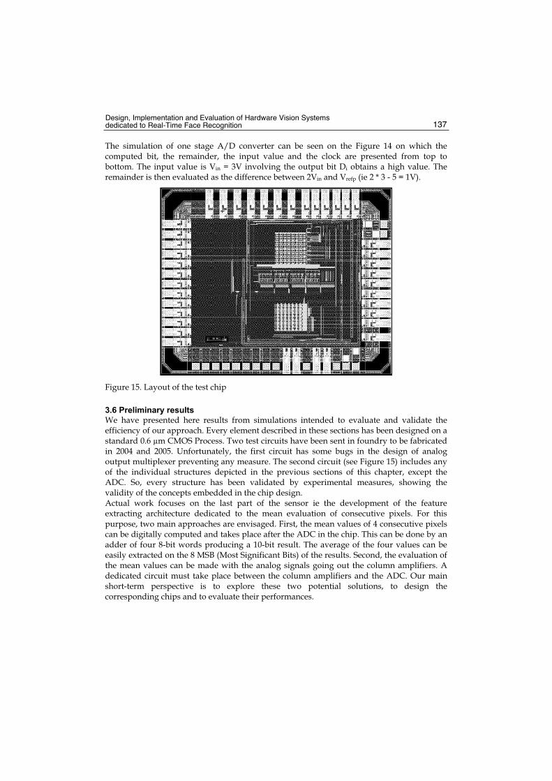
Design, Implementation and Evaluation of Hardware Vision Systems dedicated to Real-Time Face Recognition 137
The simulation of one stage A/D converter can be seen on the Figure 14 on which the computed bit, the remainder, the input value and the clock are presented from top to bottom. The input value is Vin = 3V involving the output bit Di obtains a high value. The remainder is then evaluated as the difference between 2Vin and Vrefp (ie 2 * 3 - 5 = 1V).
Figure 15. Layout of the test chip
3.6 Preliminary results
We have presented here results from simulations intended to evaluate and validate the efficiency of our approach. Every element described in these sections has been designed on a standard 0.6 μm CMOS Process. Two test circuits have been sent in foundry to be fabricated in 2004 and 2005. Unfortunately, the first circuit has some bugs in the design of analog output multiplexer preventing any measure. The second circuit (see Figure 15) includes any of the individual structures depicted in the previous sections of this chapter, except the ADC. So, every structure has been validated by experimental measures, showing the validity of the concepts embedded in the chip design. Actual work focuses on the last part of the sensor ie the development of the feature extracting architecture dedicated to the mean evaluation of consecutive pixels. For this purpose, two main approaches are envisaged. First, the mean values of 4 consecutive pixels can be digitally computed and takes place after the ADC in the chip. This can be done by an adder of four 8-bit words producing a 10-bit result. The average of the four values can be easily extracted on the 8 MSB (Most Significant Bits) of the results. Second, the evaluation of the mean values can be made with the analog signals going out the column amplifiers. A dedicated circuit must take place between the column amplifiers and the ADC. Our main short-term perspective is to explore these two potential solutions, to design the corresponding chips and to evaluate their performances.

Face Recognition 138
The next effort will be the fabrication of a real chip in a modern process such as a 130 nm CMOS technology. The main objective will be the design of a 256 x 256 pixel array with a pixel size of less than 10 μm x 10 μm. This chip will include all the necessary electronics allowing the extraction of parameters which can serve as inputs of a RBF neural network dedicated to face recognition.
4. Development of a fast panoramic face mosaicking and recognition system
Biometry is currently a very active area of research, which comprises several subdisciplines such as image processing, pattern recognition, and computer vision (Kung et al., 2005). The main goal of biometry is to build systems that can identify people from some observable characteristics such as their faces, fingerprints. Faces seem to have a particularly strong appeal for human users, in part because we routinely use facial information to recognize each other. Different techniques have been used to process faces such as neural network approaches (Howel & Buxton, 1998) eigenfaces (Turk & Pentland, 1991) and Markov chains (Slimane et al., 1999) As the recent DARPA-sponsored vendor test showed, most systems use frontal facial images as their input patterns (Phillips et al., 2003) As a consequence, most of these methods are sensitive to pose and lighting conditions. One way to override these limitations is to combine modalities (color, depth, 3-D facial surface, etc.) (Tsalakanidou et al., 2003, Hehser et al., 2003, Bowyer et al., 2004). Most 3-D acquisition systems use professional devices such as a travelling camera or a 3-D scanner (Hehser et al., 2003, Lu et al., 2004). Typically, these systems require that the subject remain immobile during several seconds in order to obtain a 3-D scan, and therefore these systems may not be appropriate for some applications, such as human-expression categorization using movement estimation, or real-time applications. Also, their cost can easily make these systems prohibitive for routine applications. In order to avoid using expensive and time-intensive 3-D acquisition devices, some face recognition systems generate 3-D information from stereo vision (Wang et al., 2003). Complex calculations, however, are needed in order to perform the required self-calibration and 2-D projective transformation (Hartly et al., 2003). Another possible approach is to derive some 3-D information from a set of face images, but without trying to reconstitute the complete 3-D structure of the face (Tsalakanidou et al., 2003). For the last ten years, our laboratory has worked on face processing and obtained results for 2-D face tracking and recognition. The goal of the present section is to describe a system that is simple and efficient and that also can potentially process 3-D faces in real time. Our method creates panoramic face mosaics, which give some 3-D surface information. The acquisition system is composed of five cameras, which together can obtain simultaneously five different views of a given face. One of its main advantages is easy setup and very low cost. This section is organized as follows. First, we describe our acquisition system. Then, we describe the method for creating panoramic face mosaics using successive linear transformations. Next, we present experimental results on panoramic face recognition. Finally, we conclude and explore possible follow-ups and improvements.
4.1 Acquisition system
Our acquisition system is composed of five Logitech 4000 USB cameras with a maximal resolution of 640 x 480 pixels. The parameters of each camera can be adjusted
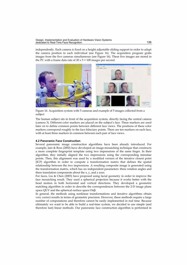
Design, Implementation and Evaluation of Hardware Vision Systems dedicated to Real-Time Face Recognition 139
independently. Each camera is fixed on a height adjustable sliding support in order to adapt the camera position to each individual (see Figure 16). The acquisition program grabs images from the five cameras simultaneous (see Figure 16). These five images are stored in the PC with a frame data rate of 20 x 5 = 100 images per second.
Figure 16. Acquisition system with 5 cameras and example of 5 images collected from a subject
The human subject sits in front of the acquisition system, directly facing the central camera (camera 3). Different color markers are placed on the subject’s face. These markers are used later on to define common points between different face views. The positions of these color markers correspond roughly to the face fiduciary points. There are ten markers on each face, with at least three markers in common between each pair of face views.
4.2 Panoramic Face Construction
Several panoramic image construction algorithms have been already introduced. For example, Jain & Ross (2002) have developed an image-mosaicking technique that constructs a more complete fingerprint template using two impressions of the same finger. In their algorithm, they initially aligned the two impressions using the corresponding minutiae points. Then, this alignment was used by a modified version of the iterative closest point (ICP) algorithm in order to compute a transformation matrix that defines the spatial relationship between the two impressions. A resulting composite image is generated using the transformation matrix, which has six independent parameters: three rotation angles and three translation components about the x, y, and z axes. For faces, Liu & Chen (2003) have proposed using facial geometry in order to improve the face mosaicking result. They used a spherical projection because it works better with the head motion in both horizontal and vertical directions. They developed a geometric matching algorithm in order to describe the correspondences between the 2-D image plane space QUV and the spherical surface space Oαβ.In general, the methods using nonlinear transformations and iterative algorithms obtain very correct results in terms of geometric precision. However, these methods require a large number of computations and therefore cannot be easily implemented in real time. Because ultimately we want to be able to build a real-time system, we decided to use simple (and therefore fast) linear methods. Our panoramic face construction algorithm is performed in
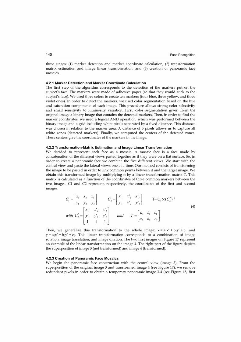
Face Recognition 140
three stages: (1) marker detection and marker coordinate calculation, (2) transformation matrix estimation and image linear transformation, and (3) creation of panoramic face mosaics.
4.2.1 Marker Detection and Marker Coordinate Calculation
The first step of the algorithm corresponds to the detection of the markers put on the subject’s face. The markers were made of adhesive paper (so that they would stick to the subject’s face). We used three colors to create ten markers (four blue, three yellow, and three violet ones). In order to detect the markers, we used color segmentation based on the hue and saturation components of each image. This procedure allows strong color selectivity and small sensitivity to luminosity variation. First, color segmentation gives, from the original image a binary image that contains the detected markers. Then, in order to find the marker coordinates, we used a logical AND operation, which was performed between the binary image and a grid including white pixels separated by a fixed distance. This distance was chosen in relation to the marker area. A distance of 3 pixels allows us to capture all white zones (detected markers). Finally, we computed the centers of the detected zones. These centers give the coordinates of the markers in the image.
4.2.2 Transformation-Matrix Estimation and Image Linear Transformation
We decided to represent each face as a mosaic. A mosaic face is a face made by concatenation of the different views pasted together as if they were on a flat surface. So, in order to create a panoramic face we combine the five different views. We start with the central view and paste the lateral views one at a time. Our method consists of transforming the image to be pasted in order to link common points between it and the target image. We obtain this transformed image by multiplying it by a linear transformation matrix T. This matrix is calculated as a function of the coordinates of three common markers between the two images. C1 and C2 represent, respectively, the coordinates of the first and second images:
111
'''
'''
)(CT'''
'''
222
111
321
321
*
2
1*
21
321
321
2
321
321
1
==
×=== −
cbacba
Tandyyyxxx
Cwith
Cyyyxxx
Cyyyxxx
C
(4)
Then, we generalize this transformation to the whole image: x = a1x’ + b1y’ + c1 and y = a2x’ + b2y’ + c2. This linear transformation corresponds to a combination of image rotation, image translation, and image dilation. The two first images on Figure 17 represent an example of the linear transformation on the image 4. The right part of the figure depicts the superposition of image 3 (not transformed) and image 4 (transformed).
4.2.3 Creation of Panoramic Face Mosaics
We begin the panoramic face construction with the central view (image 3). From the superposition of the original image 3 and transformed image 4 (see Figure 17), we remove redundant pixels in order to obtain a temporary panoramic image 3-4 (see Figure 18, first

Design, Implementation and Evaluation of Hardware Vision Systems dedicated to Real-Time Face Recognition 141
image). In order to eliminate redundant pixels, we create a cutting line that goes through two yellow markers. This panoramic image 3-4 temporarily becomes our target image. We repeat this operation for each view. First, image 2 is pasted on the temporary panoramic image 3-4 in order to obtain a new temporary panoramic image 2-3-4 (see Figure 18, second image). The corresponding transformation matrix is generated using three common violet markers. Then, we compute the transformation matrix that constructs image 2-3-4-5 (see Figure 18, third image) using two blue markers and one yellow marker. Finally, image 1 is pasted to the temporary panoramic image 2-3-4-5 with the help of two blue markers and one violet marker (see Figure 18, fourth image).
Figure 17. From left to right, Image 4 before and after the linear transformation, original image 3 and superposition of transformed image 4 and original image 3
Figure 18. Mosaicking results: image 3-4, image 2-3-4, image 2-3-4-5, and , image 1-2-3-4-5
Figure 19 displays some examples of the final panoramic face composition from five views. This composition preserves some of the face shape. For example, the chin of a human face possesses more curvature than other parts; therefore the bottom part of the panoramic face is composed of five views: 1, 2, 3, 4, and 5. On the other hand, three views (1, 3, and 5) suffice to compose the top part. Figure 19 shows final mosaic faces obtained after automatic contour cutting. For this, we first surround the panoramic face with a circle that passes by the extreme points of the ears in order to eliminate the background. Then, we replace segments of this circle by polynomial curves using extreme-point coordinates located with the help of the marker positions. Note that these ten markers allow us to link common points between five views. The coordinates of the markers are computed in the marker detection process and arranged in a table. Then, all ten markers are erased from all five views, using a simple image-processing technique (local smoothing). This table of marker coordinates is regenerated for each temporary panoramic image construction. The goal of marker elimination is to use panoramic faces for face recognition or 3-D face reconstruction. As compared to the method proposed by Liu & Chen (2003) panoramic faces obtained using our model are less precise in geometry. For example, Liu and Chen used a triangle mesh in order to represent a face. Each triangle possesses its own transformation parameters. In our system, a single transformation matrix is generated for a complete image. Liu and Chen have also established a statistical modeling containing the mean image and a number of “eigenimages” in order to represent the face mosaic. Our objective is to study an efficient and simple algorithm for later hardware implantations. Methods necessitating a large

Face Recognition 142
calculation volume and a large memory space are not adapted to embedded systems. In order to test and validate our panoramic face mosaicking algorithm, we propose, in the next sections, a study of face recognition based on the eigenface model proposed by Turk & Pentland (1991). With our method, we created a panoramic face database composed of 12 persons x 4 expressions x 2 sessions = 96 panoramic faces. The two acquisition sessions were performed over an interval of one month. The four expressions were: neutral, smile, deepened eyebrows, and eyes closed (see Figure 19). We implemented a face recognition procedure using this database.
Figure 19. Examples of panoramic faces
4.3 Face Recognition Description
Over the past 25 years, several face recognition techniques have been proposed, motivated by the increasing number of real-world applications and also by the interest in modelling human cognition. One of the most versatile approaches is derived from the statistical technique called principal component analysis (PCA) adapted to face images (Valentin et al., 1994). Such a approach has been used, for example, by Abdi (1988) and Turk & Pentland (1991) for face detection and identification. PCA is based on the idea that face recognition can be accomplished with a small set of features that best approximates the set of known facial images. Application of PCA for face recognition proceeds by first performing a PCA on a well-defined set of images of known human faces. From this analysis, a set of K principal components is obtained, and the projection of the new faces on these components is used to compute distances between new faces and old faces. These distances, in turn, are used to make predictions about the new faces. Technically, PCA on face images proceeds as follows. The K face images to be learned are represented by K vectors ak, where k is the image number. Each vector ak is obtained by concatenating the rows of the matrix storing the pixel values (here, gray levels) of the k’th face image. This operation is performed using the vec operation, which transforms a matrix into a vector (see Abdi et al. (1995) for more details).

Design, Implementation and Evaluation of Hardware Vision Systems dedicated to Real-Time Face Recognition 143
The complete set of patterns is represented by a I x K matrix noted A, where I represents the number of pixels of the face images and K the total number of images under consideration. Specifically, the learned matrix A can be expressed as A = P Δ QT where P is the matrix of eigenvectors of AAT, Q is the matrix of eigenvectors of ATA, and Δ is the diagonal matrix of singular values of A, that is, Δ=Λ1/2, with Λ, the matrix of eigenvalues of AAT and ATA. The left singular eigenvectors P can be rearranged in order to be displayed as images. In general, these images are somewhat facelike (Abdi, 1988) and they are often called eigenfaces. Given the singular vectors P, every face in the database can be represented as a weight vector in the principal component space. The weights are obtained by projecting the face image onto the left singular vectors, and this is achieved by a simple inner product operation: PROJx=XTPΔ-1 where x is a facial vector, corresponding to an example face in the training process or a test face in the recognition process. Therefore, when a new test image whose identification is required is given, its vector of weights also represents the new image. Identification of the test image is done by locating the image in the known face database whose weights have the smallest Euclidean distance from the weight of the test image. This algorithm, employed by Turk and Pentland is called the nearest neighbor classification rule.
4.4 Experimental results on Panoramic Face Recognition
For these first tests, panoramic faces were analyzed using the original 240x320-pixel image (spatial representation) without preprocessing. The database consisted of 12 persons x 4 expressions x 2 1sessions = 96 panoramic faces, and was divided into two subsets. One subset served as the training set, and the other subset as the testing set. As illustrated in Figure 19, all these panoramic faces possess a uniform background, and the ambient lighting varied according to the daylight. From the panoramic face database, one, two, three, or four images were randomly chosen for each individual in order to create the training set (number of patterns for learning per individual, p=1, 2, 3, 4). The rest of the panoramic faces were used in order to test the face recognition method. For example, when p=1, the total number of training examples is equal to 1 x 12 persons = 12, and the number of test samples for recognition is equal to 96 12=84. Therefore, for each individual, only one panoramic face is learned in order to recognize seven other images of this person. Several executions of our MATLAB program were run for each value of p, using randomly chosen training and testing sets. Then we computed the mean performance. Using the nearest neighbour classification rule, the panoramic face identity test is done by locating the closest image in the known face database. Therefore, the system can make only confusion errors (i.e., associating the face of one person with a test face of another). Correct panoramic face recognition rates go from 70 % when p=1 to 93.2% when p=4. We added a discriminant analysis stage in the face recognition process so as to determine the number of necessary eigenvectors. This analysis, called the jackknife (Yang & Robinson, 2001) reorders eigenvectors, not according to their eigenvalues, but according to their importance for identification. Specifically, we computed the ratio of the between-group inertia to the within-group inertia for each eigenvector. This ratio expresses the quality of the separation of the identity of the subject performed by this eigenvector. The eigenvector with the largest ratio performs the best identity separation, the eigenvector with the second largest ratio performs second best, etc. We observe that it suffices to use only 23

Face Recognition 144
eigenvectors to reach the maximum recognition rate (93.2%). Additional eigenvectors do not add to the quality of the identification. We also tested the frequential behavior of our recognition system. We can observe that the frequential spectra of a panoramic face are well centered at low frequencies. This allows us to apply a lowpass filter in order to reduce the size of the data set to process. Only 80 x 80 FFT amplitude values of low frequencies were used for the recognition system.
Figure 20. (a) original image, (b) original image with added Gaussian noise, (c) FFT image using the spectrum amplitude of (b) and the phase of (a) and (d) FFT image using the spectrum amplitude of (a) and the phase of (b)
We applied the same training and testing process as used in spatial representation. We obtain a better recognition rate with the frequential representation (97.5%) than with the spatial representation (93.2%). This advantage of the frequential representation is due to the fact that for face images, the spectrum amplitude is less sensitive to noise than the spectrum phase. We confirmed this interpretation by using a panoramic face image to which noise was added. Figure 20(a) shows a original panoramic face. Figure 20 (b) displays the same panoramic face image with added noise. We first obtained the FFTs of these two images and then their inverse FFTs in the two following manners: (1) using the spectrum amplitude of the noised image and the spectrum phase of the original image (see Figure 20-c) and (2) using the spectrum phase of the noised image and the spectrum amplitude of the original image (see Figure 20-d). These results show that the face obtained with the first configuration is closer to the original face than the face obtained with the second configuration. This confirms that the spectrum amplitude is less sensitive to noise than the spectrum phase.
4.5 Panoramic face recognition with negative samples
In order to evaluate the behavior of our system for unknown people, we added four people to the test database. These panoramic faces were obtained as described in Sec. 4.2. Table 4 displays the performance of different tests. In order to reject these unknown faces, we established a threshold of Euclidean distance. Because we are working on applications of typical access control, where confusion is more harmful than nonrecognition, we decided to use a severe acceptance threshold in order to reject intruders. Note that the acceptance threshold is constant for all tests. Efficiency is defined as follows: • Recognition: Correct recognition of a panoramic face. • Nonrecognition: A panoramic face has not been recognized. • Confusion: A panoramic face is confused with an intruder. These performance results are obtained using the frequential representation and show that performance declines in comparison with tests without negative samples.

Design, Implementation and Evaluation of Hardware Vision Systems dedicated to Real-Time Face Recognition 145
Num
ber o
f tr
aini
ngex
ampl
es p
er
indi
vidu
al p
Tota
l num
ber
of tr
aini
ng
exam
ples
Num
ber o
f ei
genv
ecto
rsus
ed
Num
ber o
f te
sts
for
reco
gniti
on
Non
reco
gniti
on
rate
(%)
Con
fusi
onra
te (%
)
Reco
gniti
on
rate
(%)
1 12 8 116 25.4 5.85 68.75 2 24 13 104 12.74 4 83.26 3 36 18 92 7.58 3.5 88.92 4 48 24 80 4.82 2.8 92.38
Table 4. Results of panoramic face recognition with negative samples
4.6 Discussion
In this section, we have proposed a fast and simple method for panoramic face mosaicking. The acquisition system consists of several cameras followed by a series of fast linear transformations of the images. The simplicity of the computations makes it possible to envisage real-time applications. In order to test the recognition performance of our system, we used the panoramic faces as input to a recognition system based on PCA. We tested two panoramic face representations: spatial and frequential. We found that a frequential representation gives the better performance, with a correct recognition rate of 97.46%, versus 93.21% for spatial representation. An additional advantage of the frequential representation is that it reduces the data volume to be processed and this further accelerates the calculation speed. We used negative samples for the panoramic face recognition system, and the correct recognition rate was 92.38%.Experimental results show that our fast mosaicking system provides relevant 3-D facial surface information for recognition application. The obtained performance is very close or superior to published levels (Howell & Buxton, 1998, Slimane et al., 1999, Tsalakanidou et al., 2003). In the future, we plan to simplify our acquisition system by replacing the markers with a structured light. We also hope to use our system without markers. For this, we will detect control points on faces (corners, points of maximum curvature, etc.). Another line of development is to improve the geometry quality of our panoramic face mosaic construction (Liu & Chen, 2003, Puech et al., 2001). For this, we will use realistic human face models. We are also exploring processing panoramic face recognition using other classifiers with more variable conditions.
5. Conclusions
In this chapter, we have presented three dedicated systems to face recognition developed by our research team since 2002. Our main objective was motivated by the implementation on embedded systems of efficient models of unconstrained face tracking and identity verification in arbitrary scenes. The main goal of these various systems is to provide efficient algorithms that only require few hardware in order to obtain high success rates of face recognition with high real time constraints. The first system is a real time vision system that allows us to localize faces in video sequences and verify their identity. These processes are image processing techniques and
Face Recognition 146
the radial basis function (RBF) neural network approach. The robustness of this system has been evaluated quantitatively on eight video sequences. We have also described three hardware implementations of our model on embedded systems based, respectively, on field programmable gate array (FPGA), zero instruction set computer (ZISC) chips, and digital signal processor (DSP). For each configuration, we have analyzed the algorithm complexity and present results of implementations in terms of resources and processing speed. The main results of these first implementations have highlighted the need of a dedicated hardware such as an artificial retina embedding low level image processing in order to extract input vectors of the RBF neural network. Such a system could unload a consequent calculation part of FPGA. So, the second part of the chapter was devoted to the description of the principles of an adequate CMOS sensor. For this purpose, a current mode CMOS active sensor has been designed using an array of pixels that are amplified by using current mirrors of column amplifiers. This circuit is simulated using Mentor GraphicsTMsoftware with parameters of a 0.6 μm CMOS process. The circuit is able to realise captures of subwindows at any location and any size in the whole image and computes mean values of adjacent pixels which can serve as inputs of the RBF network. In the last section of this chapter, we present some new results on a system that performs mosaicking of panoramic faces. Our objective was to study the feasibility of panoramic face construction in real time. We built a simple acquisition system composed of five standard cameras, which together can take simultaneously five views of a face at different angles. Then, we chose an easily hardware-achievable algorithm, consisting of successive linear transformations, in order to compose a panoramic face from these five views. In order to validate our system, we also conducted a preliminary study on panoramic face recognition, based on the principal-component method. Experimental results show the feasibility and viability of our system and allow us to envisage later a hardware implementation.
6. References
Abdi, H. (1988). A generalized approach for connectionist auto-associative memories: interpretation, implications and illustration for face processing, in Artificial Intelligence and Cognitive Sciences, J. Demongeot (Ed.), Manchester Univ. Press.
Abdi, H.; Valentin, D.; Edelman, B. & O’Toole, A. (1995). More about the difference between men and women: evidence from linear neural networks and the principal component approach, Perception vol 24, pp 539–562.
Aw, C. & Wooley, B. (1996) .A 128x128 pixel standard cmos image sensor with electronic shutter,. IEEE Journal of Solid State Circuits, vol. 31, no. 12, pp. 1922-1930.
Baker, R.; Li, H.; & Boyce; D. (1998). CMOS Circuit Design Layout and Simulation. New-York: IEEE Press.
Bowyer, K.; Chang, K. & Flynn, P. (2004). A survey of 3D and multi- modal 3D+2D face recognition, in Proc. Int. Conf. on Pattern Recognition (ICPR).
Buhmann, J.; Lades, M. & Eeckmann, F. (1994). Illumination-invariant face recognition with a contrast sensitive silicon retina, in Advances in Neural Information Processing Systems (NIPS). New York: Morgan Kaufmann, 1994, vol. 6, pp. 769–776.
Coulombe, J.; Sawan, M. & Wang, C. (2000).Variable resolution CMOS current mode active pixel sensor. in IEEE International Symposium on Circuits and Systems.
Férand, R.et al. (2001). A fast and accurate face detector based on neural networks, IEEETrans. Pattern Anal. Mach. Intell., vol. 23, pp. 42–53.

Design, Implementation and Evaluation of Hardware Vision Systems dedicated to Real-Time Face Recognition 147
Hartly, R. & Zisserman, A. (2003). Multiple View Geometry in Computer Vision, 2nd ed., Cambridge Univ. Press
Hehser, C.; Srivastava, A. & Erlebacher, G. (2003). A novel technique for face recognition using range imaging, in Proc. 7th Int. Symp. On Signal Processing and Its Applications.
Howell, A. & Buxton, H. (1998). Learning identity with radial basis function networks, Neurocomput., vol. 20, pp. 15–34.
Huang, Y. & Horsney, R. (2003). Current-mode cmos image sensor using lateral bipolar phototransistors,. IEEE Trans. on Electron Devices, vol. 50, no. 12, pp. 2570-2573.
Jain, A. & Ross, A. (2002). Fingerprint mosaicking, in Proc. IEEE Int. Conf. on Acoustics, Speech, and Signal Processing (ICASSP).
Kemeny, S.; Mathias, L. & Fossum, E. (1997). Multiresolution image sensor, IEEE Transactions on Circuit and System for Video Technology, vol. 7, no. 4, pp. 575-583.
Kobayashi, K. (2001). Mobile terminals and devices technology for the 21st century, Spec.Rev. Paper—New Start 21st Century: NEC Res. Develop., vol. 42, no. 1.
Koh, L.; Ranganath, S. & Venkatesh, Y. (2002). An integrated automatic face detection and recognition system, Pattern Recogn., vol. 35, pp. 1259–1273.
Kung, S.; Mak, M. & Lin S. (2005), Biometric Authentification: A Machine Learning Approach,Prentice-Hall, Upper Saddle River, NJ
Lewis, S.; Fetterman, H.; Gross, G.; Ramachandran, R. & Viswanathan T. (1992), .10-b 20-Msample/s analog-to-digital converter. IEEE Journal on Solid-States Circuits, vol. 27, no. 3, pp. 351-358.
Lindblad, T.et al. (1995). Implementating of the new zero instruction set computer (ZISC036) from IBM for a Higgs Search, Nucl. Instrum. Methods, vol. A357.
Liu, H. (1998). An automatic human face recognition system, Opt. Lasers Eng., vol. 30, pp. 305–314.
Liu, X. & Chen, T. (2003). Geometry-assisted statistical modeling for face mosaicing, in IEEE Int. Conf. on Image Processing (ICIP), Vol. 2, pp.883–886.
Lu, X.; Colbry, D. & Jain, A. (2004). Three-dimensional model based face recognition, in Proc. Int. Conf. on Pattern Recognition, pp. 362–366.
Matsumoto, Y. & Zelinsky, A. (2000). An algorithm for real-time stereo vision implementation of head pose and gaze direction measurement, in Proc. 4th IEEE Int. Conf. Automatic Face and Gesture Recognition, Grenoble, France, pp. 499–504.
Nakamura, J.; Pain, B; Nomoto, T.; Nakamura, T. & E. Fossum. (1997). Onfocal plane signal processing for current-mode active pixel sensors. IEEE Transaction on Electrons Devices, vol. 44, no. 10, pp. 1747-1758.
Park, I. & Sandberg, I. (1991). Universal approximation using radial basis function networks, Neural Computat., vol. 3, pp. 246–257.
Pérez-Uribe, A. & Sanchez, E. (1996). FPGA implementation of an adaptable- size neural network, in Proc. Int. Conf. Artificial Neural Networks ICANN’96, Bochum, Germany.
Phillips, P.; Grother, P.; Micheals, R.; Blackburn, D.; Tabassi, E. & Bone, J. (2003). Face recognition vendor test 2002, presented at IEEE International Workshop on Analysis and Modeling of Faces and Gestures (AMFG).
Puech, W.; Bors, A.; Pitas, I. & Chassery, J.-M. (2001). Projection distortion analysis for flattened image mosaicking from straight uniform generalized cylinders, Pattern Recogn. vol 34, pp 1657–1670.

Face Recognition 148
Rosenblum, M.; Yacoob, Y. & Davis, L. (1996). Human expression recognition from motion using a radial basis function network architecture, IEEE Trans. Neural Networks, vol. 7, pp. 1121–1138.
Rowley, H.; Baluja, S. & Kanade, T. (1998). Neural network-based face detection, IEEE Trans. Pattern Anal. Mach. Intell., vol. 20, pp. 23–38.
Sim, T.et al. (2000). Memory-based face recognition for visitor identification, in Proc. 4thIEEE Int. Conf. Automatic Face and Gesture Recognition, Grenoble, France, pp. 26–30.
Skrbek, M. (1999). Fast neural network implementation, Neural Network World, vol. 5, pp. 375–391.
Slimane, M.; Brouard, T.; Venturini, G. & Asselin de Beauville, J. P. (1999). Unsupervised learning of pictures by genetic hybridization of hidden Markov chain, SignalProcess. vol 16, no 6, 461–475.
Sonkusale, S.; Speigel, J. & Nagaraj, K. (2001) .Background digital error correction technique for pipelined ADC,. In Proc of IEEE ISCAS, vol 1, pp 408-411.
Tabet, M. & Hornsey, R. (2001). Cmos image sensor camera with focal plane edge detection,. in Canadian Conference on Electrical and Computer Engineering, vol. 2, pp. 1129-1133.
Thomson, D. & Wooley, B. (2001).A 15-b pipelined cmos _oating point a/d converter,. IEEE Journal on Solid-States Circuits, vol. 36, no. 2, pp. 299-303.
Tsalakanidou, F.; Tzovaras, D. & Strintzis, M. (2003). Use of depth and colour eigenfaces for face recognition, Pattern Recogn. Lett. vol 24, pp 1427–1435.
Turk, M. & Pentland, A. (1991). Eigenfaces for recognition, J. Cogn Neurosci,. vol 3, pp 71–86. Valentin, D.; Abdi, H.; O’Toole, A. & Cottrell, G. (1994). Connectionist models of face
processing: a survey, Pattern Recogn. vol 27, pp 1208–1230. Wang, J.; Venkateswarlu, R. & Lim, E. (2003). Face tracking and recognition from stereo
sequence, Comput. Sci. vol 2688, pp 145–153. Yang, F. & Paindavoine, M. (2003) , Implementation of a RBF neural network on embedded
systems: real time face tracking and identity verification, IEEE Trans. Neural Netw. vol 14, no 5, pp 1162–1175.
Yang, M.; Kriegman, D. & Ahuja, N. (2001). Detecting faces in images: A survey, IEEE Trans. Pattern Anal. Mach. Intell., vol. 23, pp. 42–53.
Yang, M. & Robinson D. (1986). Understanding and Learning Statistics by Computer, World Scientific, Singapore.
Yeh, Y. & Lee, C. (1999). Cost effective VLSI architectures and buffer size optimization for full search block matching algorithms, IEEE Trans. VLSI Syst., vol. 7, pp. 345–358,

9
Face and Gesture Recognition for Human-Robot Interaction
Dr. Md. Hasanuzzaman1 and Dr. Haruki Ueno2
1Department of Computer Science & Engineering, University of Dhaka 2National Institute of Informatics, The Graduate University for Advanced Studies, Tokyo
1Bangladesh, 2Japan
1. Introduction
This chapter presents a vision-based face and gesture recognition system for human-robot interaction. By using subspace method, face and predefined hand poses are classified from the three largest skin-like regions that are segmented using YIQ color representation system. In the subspace method we consider separate eigenspaces for each class or pose. Face is recognized using pose specific subspace method and gesture is recognized using the rule-based approach whenever the combinations of three skin-like regions at a particular image frame satisfy a predefined condition. These gesture commands are sent to robot through TCP/IP wireless network for human-robot interaction. The effectiveness of this method has been demonstrated by interacting with an entertainment robot named AIBO and a humanoid robot Robovie. Human-robot symbiotic systems have been studied extensively in recent years, considering that robots will play an important role in the future welfare society [Ueno, 2001]. The use of intelligent robots encourages the view of the machine as a partner in communication rather than as a tool. In the near future, robots will interact closely with a group of humans in their everyday environment in the field of entertainment, recreation, health-care, nursing, etc. In human-human interaction, multiple communication modals such as speech, gestures and body movements are frequently used. The standard input methods, such as text input via the keyboard and pointer/location information from a mouse, do not provide a natural, intuitive interaction between humans and robots. Therefore, it is essential to create models for natural and intuitive communication between humans and robots. Furthermore, for intuitive gesture-based interaction between human and robot, the robot should understand the meaning of gesture with respect to society and culture. The ability to understand hand gestures will improve the naturalness and efficiency of human interaction with robot, and allow the user to communicate in complex tasks without using tedious sets of detailed instructions. This interactive system uses robot eye’s cameras or CCD cameras to identify humans and recognize their gestures based on face and hand poses. Vision-based face recognition systems have three major components: image processing or extracting important clues (face pose and position), tracking the facial features (related position or motion of face and hand poses), and face recognition. Vision-based face recognition system varies along a number of

Face Recognition 150
dimensions: number of cameras, speed and latency (real-time or not), structural environment (restriction on lighting conditions and background), primary features (color, edge, regions, moments, etc.), etc. Multiple cameras can be used to overcome occlusion problems for image acquisition but this adds correspondence and integration problems. The aim of this chapter is to present a vision-based face and hand gesture recognition method. The scope of this chapter is versatile. Segmentation of face and hand regions from the cluttered background, generation of eigenvectors and feature vectors in training phase, classification of face and hand poses, recognizes the user and gesture. In this chapter we present a method for recognizing face and gestures in real-time combining skin-color based segmentation and subspace-based patterns matching techniques. In this method three larger skin like regions are segmented from the input images using skin color information from YIQ color space, assuming face and two hands may present in the images at the same time. Segmented blocks are filtered and normalized to remove noises and to form fixed size images as training images. Subspace method is used for classifying hand poses and face from three skin-like regions. If the combination of three skin-like regions at a particular frame matches with the predefined gesture then corresponding gesture command is generated. Gesture commands are being sent to robots through TCP-IP network and their actions are being accomplished according to user’s predefined action for that gesture. In this chapter we have also addressed multi directional face recognition system using subspace method. We have prepared training images in different illuminations to adapt our system with illumination variation. This chapter is organized as follows. Section 2 focuses on the related research regarding person identification and gesture recognition. In section 3 we briefly describe skin like regions segmentation, filtering and normalization techniques. Section 4 describes subspace method for face and hand poses classification. Section 5 presents person identification and gesture recognition method. Section 6 focuses on human-robot interaction scenarios. Section 7 concludes this chapter and focuses on future research.
2. Related Work
This section briefly describes the related research on computer vision-based systems that include the related research on person identification and gesture recognition systems. Numbers of approaches have been applied for the visual interpretation of gestures to implement human-machine interaction [Pavlovic, 1997]. Major approaches are focused on hand tracking, hand poster estimation or hand pose classification. Some studies have been undertaken within the context of particular application: such as using a finger as a pointer to control TV, or manipulated Augmented desks. There are large numbers of household machine that can take benefit from the intuitive gesture understanding, such as: Microwave, TV, Telephone, Coffee maker, Vacuum cleaner, Refrigerator, etc. The aged/disable people can access such kind of machine if its have intuitive gesture understanding interfaces. Computer vision supports a wide range of human tasks including, recognition, navigation, communication, etc. Using computer vision to sense and perceive the user in an HCI or HRI context is often called vision-based interaction or vision-based interface (VBI). In recent years, there has been increased research on practical vision-based interaction methods, due to availability of vision-based software, and inexpensive and fast enough computer vision related hardware components. As an example of VBI, hand pose or gesture recognition offers many promising approaches for human-machine interaction (HMI). The primary goal

Face and Gesture Recognition for Human-Robot Interaction 151
of the gesture recognition researches is to develop a system, which can recognize specific user and his/her gestures and use them to convey information or to control intelligent machine. Locating the faces and identifying the users is the core of any vision-based human-machine interface systems. To understand what gestures are, brief overviews of other gesturer researchers are useful.
2.1 Face Detection and Recognition
In the last few years, face detection and person identification attracts many researchers due to security concern; therefore, many interesting and useful research demonstrations and commercial applications have been developed. A first step of any face recognition or vision-based person identification system is to locate the face in the image. Figure 1 shows the example scenarios of face detection (partly of the images are taken from Rowley research paper [Rowley, 1997]). After locating the probable face, researchers use facial features (eyes, nose, nostrils, eyebrows, mouths, leaps, etc.) detection method to detect face accurately [Yang, 2000]. Face recognition or person identification compares an input face image or image features against a known face database or features databases and report match, if any. Following two subsections summarize promising past research works in the field of face detection and recognition.
2.1.1 Face Detection
Face detection from a single image or an image sequences is a difficult task due to variability in pose, size, orientation, color, expression, occlusion and lighting condition. To build a fully automated system that extracts information from images of human faces, it is essential to develop efficient algorithms to detect human faces. Visual detection of face has been studied extensively over the last decade. There are many approaches for face detection. Face detection researchers summarized the face detection work into four categories: template matching approaches, feature invariant approaches, appearance-based approaches and knowledge-based approaches [Yang, 2002]. Such approaches typically rely on a static background, so that human face can be detected using image differencing. Many researches also used skin color as a feature and leading remarkable face tracking as long as the lighting conditions do not varies too much [Dai, 1996], [Crowley, 1997]. Template Matching Approaches In template matching methods, a standard template image data set using face images is manually defined. The input image is compared with the template images and calculated correlation coefficient or/and minimum distances (Manhattan distance, Euclidian distance, Mahalanobis distance, etc.). The existence of face is determined using the maximum correlation coefficient value and/or minimal distance. For exact matching correlation coefficient is one and minimum distance is zero. This approach is very simple and easy to implement. But recognition result depends on the template images size, pose, orientation, shape and intensity. Sakai et. al. [Sakai, 1996] used several sub-templates for the eyes, nose, mouth and face contour to model a face which is defined in terms of line spaces. From the input images lines are extracted based on greatest gradient change and then matched against the sub-templates. The correlation between sub-images and contour templates are computed first to locate the probable location of faces. Then matching with the other sub-templates is performed at the probable face location.

Face Recognition 152
Tsukamoto et. al. [Tsukamoto, 1994] presents a qualitative model for face [QMF]. In their model each sample image is divided into N blocks and qualitative features (‘lightness’ and ‘edgeness’) are estimated for each block. This blocked template is used to estimate “faceness” at every position of an input image. If the faceness measure is satisfied the predefined threshold then the face is detected. We have developed a face detection method using the combination of correlation coefficient and Manhattan distance features, calculated from multiple face templates and test face image [Hasanuzzaman, 2004a]. In this method three larger skin-like regions are segmented first. Then segmented images are normalized to match with the size and type of the template images. Correlation coefficient is calculated using equation (1),
/t t tM Pα = (1) where, Mt is total number of matched pixels (white pixels with white pixels and black pixels with black pixels) with the tth template, Pt is total number of pixels in the tth template and t, is a positive number. For exact matching αt is 1, but for practical environment we have selected a threshold value for αt (0<αt 1) through experiment considering optimal matching.
(a) Single face detection
(b) Multiple faces detection Figure 1. Examples of face detection scenarios [Rowley, 1997]

Face and Gesture Recognition for Human-Robot Interaction 153
Minimum distance can be calculated by using equation (2),
1
{ | |}x y
t tI Gδ×
= − (2)
where, I(x,y) is the input image and G1(x,y), G2(x,y),----------,Gt(x,y) are template images. For exact matching δt is 0, but for practical environment we have selected a threshold value for δt through experiment considering optimal matching. If the maximum correlation coefficient and the minimum distance qualifier support corresponding specific threshold values then that segment is detected as face and the center position of the segment is use as the location of the face. Miao et. al. [Miao, 1999] developed a hierarchical template matching method for multi-directional face detection. At the first stage, an input image is rotated from -20º to +20º in step of 5º. A multi-resolution image hierarchy is formed and edges are extracted using Laplacian operator. The face template consists of the edges produced by six facial components: two eyebrows, two eyes, nose and mouth. Finally, heuristics are applied to determine the existence of face. Yuille et. al. [Yuille, 1992] used deformable template to model facial features that fit a priori elastic model to facial features. In this approach, facial features are described by parameterized template. An energy function is defined to link edges, peaks, and valleys in the input image to corresponding parameters in the template. The best fit of the elastic model is found by minimizing an energy function of the parameters. Feature Invariant Approaches There are many methods to detect facial features (mouth, eyes, eyebrows, lips, hair-line, etc.) individually and from their geometrical relations to detect the faces. Human face skin color and texture also used as features for face detection. The major limitations with these feature-based methods are that the image features are corrupted due to illumination, noise and occlusion problem. Sirohey proposed a face localization method from a cluttered background using edge map (canny edge detector) and heuristics to remove and group edges so that only the ones on the face contour are preserved [Sirohey, 1993]. An ellipse is then fit to the boundary between the head region and the background. Chetverikov et. al. [Chetverikov, 1993] presented face detection method using blobs and streaks. They used two black blobs and three light blobs to represent eyes, cheekbones and nose. The model uses streaks to represent the outlines of the faces, eyebrows and lips. Two triangular configurations are utilized to encode the spatial relationship among the blobs. A low resolution Laplacian image is generated to facilitate blob detection. Next, the image is scanned to find specific triangular occurrences as candidates. A face is detected if streaks are identified around the candidates. Human faces have a distinct texture that can be separated them from other objects. Augusteijn et. al. [Augusteijn, 1993] developed a method that infers the presence of face thorough the identification of face like templates. Human skin color has been proven to be an effective feature for face detections, therefore many researchers has used this feature for probable face detection or localization [Dai 1996], [Bhuiyan, 2003], [Hasanuzzaman 2004b]. Recently, many researchers are combining multiple features for face localization and detection and those are more robust than single feature based approaches. Yang and Ahuja [Yang, 1998] proposed a face detection method based on color, structure and geometry.

Face Recognition 154
Saber and Tekalp [Saber, 1998] presented a frontal view-face localization method based on color, shape and symmetry. Darrel et. al. [Darrel, 2000] integrated stereo, color and pattern detection method to track the person in real time. Appearance-Based Approaches Appearance-based methods use training images and learning approaches to learn from the known face images. These approaches rely on the statistical analysis and machine learning techniques to find the relevant characteristics of face and non-face images. There are many researchers using appearance-based methods.Turk et. al. [Turk, 1991] applied principal component analysis to detect and recognize face. From the training face images they generated the eigenfaces. Face images and non-face images are projected onto the eigenspaces; form feature vectors and clustered the images based on separation distance. To detect the presence of a face from an image frame, the distance between the known face space and all location in the images are calculated. If the minimum distance satisfied the faceness threshold values then the location is identified as face. These approaches are widely used by the many researchers. Knowledge-Based Approaches These methods use the knowledge of the facial features in top down approaches. Rules are used to describe the facial features and their relations. For example, a face is always consists of two eyes, one nose and a mouth. The relationship is defined using relative distances and positions among them. For example, the center of two eyes are align on the same line, the center points of two eyes and mouth form a triangular. Yang and Huang [Yang, 1994] used hierarchical knowledge-based method to detect face. In this method they used three layers of rules. At the first level, all possible face candidates are found by scanning a mask window (face template) over the input images, and applying a set of rules at each location. At the second level, histogram equalization and edge detection is performed on candidate faces. At the third level, using rules facial feature are detected individually and using the pre-knowledge of their relation, detect the actual faces. Kotropoulous [Kotropoulous, 1997] and other also presented rule-based face localization method.
2.1.2 Face Recognition
During the last few years face recognition has received significant attention from the researchers [Zhao, 2003] [Chellappa, 1995]. Research on automatic machine- based face recognition has started in the 1970s [Kelly 1970]. Figure 2 shows an example of face recognition scenario. The test face image (preprocessed) is matched with the face images of known persons in the database. If the face is sufficient close (nearest and support predefined threshold) to any one of the face classes, then corresponding person is identified, otherwise the person is unknown. Zhao [Zhao, 2003] et. al. have summarized the past recent researches on face recognition methods with three categories: Holistic matching methods, Feature-based matching methods and Hybrid methods. Holistic Methods These methods use the whole face region as the raw input for the recognition unit. One of the most widely used representations of the face recognition is eigenfaces, which are based on principal component analysis (PCA). The eigenface algorithm uses the principal component analysis (PCA) for dimensionality reduction and to find the vectors those are best account for the distribution of face images within the entire face image spaces. Using
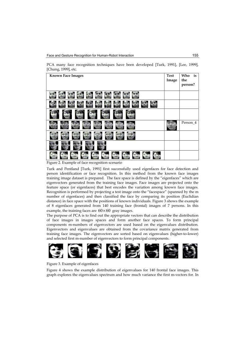
Face and Gesture Recognition for Human-Robot Interaction 155
PCA many face recognition techniques have been developed [Turk, 1991], [Lee, 1999], [Chung, 1999], etc.
Known Face Images Test Image
Who is theperson?
Person_4
Figure 2. Example of face recognition scenario
Turk and Pentland [Turk, 1991] first successfully used eigenfaces for face detection and person identification or face recognition. In this method from the known face images training image dataset is prepared. The face space is defined by the “eigenfaces” which are eigenvectors generated from the training face images. Face images are projected onto the feature space (or eigenfaces) that best encodes the variation among known face images. Recognition is performed by projecting a test image onto the “facespace” (spanned by the m number of eigenfaces) and then classified the face by comparing its position (Euclidian distance) in face space with the positions of known individuals. Figure 3 shows the example of 8 eigenfaces generated from 140 training face (frontal) images of 7 persons. In this example, the training faces are 60 60× gray images. The purpose of PCA is to find out the appropriate vectors that can describe the distribution of face images in images spaces and form another face spaces. To form principal components m-numbers of eigenvectors are used based on the eigenvalues distribution. Eigenvectors and eigenvalues are obtained from the covariance matrix generated from training face images. The eigenvectors are sorted based on eigenvalues (higher-to-lower) and selected first m-number of eigenvectors to form principal components.
Figure 3. Example of eigenfaces
Figure 4 shows the example distribution of eigenvalues for 140 frontal face images. This graph explores the eigenvalues spectrum and how much variance the first m-vectors for. In

Face Recognition 156
most cases the number of eigenvectors that account for variance somewhere in the 65%-90% range.Independent component analysis (ICA) is similar to PCA except that the distributions of the components are designed to be non-Gaussian. The ICA separates the high-order moments of the input in addition to the second order moments utilized in PCA. Bartlett et. al. [Bartlett, 1998] used ICA methods for face recognition and reported satisfactory recognition performance.Face recognition system using Linear Discriminant Analysis (LDA) or Fisher Linear Discriminant Analysis (FDA) has also been very successful. In Fisherface algorithm by defining different classes with different statistics, the images in the learning set are divided in the corresponding classes [Belhumeur, 1997]. Then, the techniques similar to those used in eigenface algorithm are applied for face classification or person identification.
Number of Eigenfaces Figure 4. Example of eigenvectors spectrum for 140 eigenfaces Feature-Based Matching Methods In these methods facial features such as the eyes, lips, nose and mouth are extracted first and their locations and local statistics (geometric shape or appearance) are fed into a structural classifier. Kanade developed one of the earliest face recognition algorithms based on automatic facial feature detection [Kanade, 1977]. By localizing the corner of the eyes, nostrils, etc., in frontal views, that system compares parameters for each face, which were compared (using Euclidian distance metric) against the parameters of known person faces. One of the most successful of these methods is the Elastic Bunch Graph Matching (EBGM) system [Wiskott, 1997]. Other well-known methods in these systems are Hidden Markov Model (HMM) and convolution neural network [Rowley, 1997]. System based on EBGM approach have been applied to face detection and extraction, pose estimation, gender classification, sketch image based recognition and general object recognition.
Var
ianc
e of
Eig
enva
lues

Face and Gesture Recognition for Human-Robot Interaction 157
Hybrid Approaches These approaches use both holistic and features based approaches. These methods are very similar to human perception consider whole image and features individually at a time. Chung et. al. [Chung, 1999] combined Gabor Wavelet and PCA based approaches for face recognition and reported better accuracy than each of individual algorithm. Pentland et. al.[Pentland, 1994] have used both global eigenfaces and local eigenfeatures (eigeneyes, eigenmouth and eigennose) for face recognition. This method is robust against face images with multiple views.
2.2 Gesture Recognition and Gesture-Based Interface
Gestures are expressive meaningful body motions i.e., physical movements of the hands, arms, fingers, head, face or other parts of the body with the intent to convey information or interact with the environment [Turk, 2000]. People all over the world use their hands, head and other parts of the body to communicate expressively. The social anthropologists Edward T. Hall claims 60% of all our communications are nonverbal [Imai, 2004]. Gestures are used for everything from pointing at a person or an object to change the focus of attention, to conveying information. From the biological and sociological perspective, gestures are loosely defined, thus, researchers are free to visualize and classify gestures as these fit. Biologists define “gesture” broadly, stating, “the notion of gesture is to embrace all kinds of instances where an individual engages in movements whose communicative intent is paramount, manifest and openly acknowledged” [Nespoulous, 1986]. Gestures associated with speech are referred to as gesticulation. Gestures, which function independently of speech, are referred to as autonomous gestures. Autonomous gestures can be organized into their own communicative language, such as American Sign Language (ASL). Autonomous gesture can also represent motion commands to use in communication and machine control. Researchers are usually concerned with gestures those are directed toward the control of specific object or the communication with a specific person or group of people. Gesture recognition is the process by which gestures made by the user are make known to the intelligence system. Approximately in the year 1992 the first attempts were made to recognize hand gestures from color video signals in real-time. It was the year, when the first frame grabbers for color video input were available, that could grab color images in real time. As color information improves segmentation and real time performance is a prerequisite for human-computer interaction, this obviously seems to be the start of development of gesture recognition. Two approaches are commonly used to recognize gestures, one is a gloved-base approach [Sturman, 1994] and another is a vision-based approach [Pavlovic, 1997].
2.2.1 Glove-Based Approaches
A common technique is to instrument the hand with a glove, which is equipped with a number of sensors, which provide information about hand position, orientation and flex of the fingers. The first commercially available hand tracker is the ‘Dataglove’ [Zimmerman, 1987]. The ‘Dataglove’ could measure each joint bend to an accuracy of 5 to 10 degrees, could classify hand pose correctly, but not the sideways movement of the fingers. The second hand tracker, ‘CyberGlove’ developed by Kramer [Kramer, 1989] uses strain gauges placed between the fingers to measure abduction as well as more accurate bend sensing.
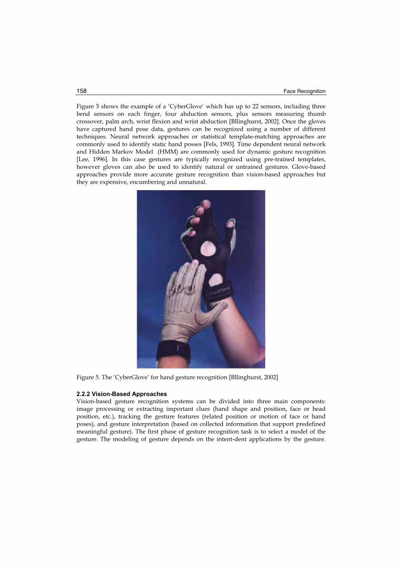
Face Recognition 158
Figure 5 shows the example of a ‘CyberGlove’ which has up to 22 sensors, including three bend sensors on each finger, four abduction sensors, plus sensors measuring thumb crossover, palm arch, wrist flexion and wrist abduction [Bllinghurst, 2002]. Once the gloves have captured hand pose data, gestures can be recognized using a number of different techniques. Neural network approaches or statistical template-matching approaches are commonly used to identify static hand posses [Fels, 1993]. Time dependent neural network and Hidden Markov Model (HMM) are commonly used for dynamic gesture recognition [Lee, 1996]. In this case gestures are typically recognized using pre-trained templates, however gloves can also be used to identify natural or untrained gestures. Glove-based approaches provide more accurate gesture recognition than vision-based approaches but they are expensive, encumbering and unnatural.
Figure 5. The ‘CyberGlove’ for hand gesture recognition [Bllinghurst, 2002]
2.2.2 Vision-Based Approaches
Vision-based gesture recognition systems can be divided into three main components: image processing or extracting important clues (hand shape and position, face or head position, etc.), tracking the gesture features (related position or motion of face or hand poses), and gesture interpretation (based on collected information that support predefined meaningful gesture). The first phase of gesture recognition task is to select a model of the gesture. The modeling of gesture depends on the intent-dent applications by the gesture.

Face and Gesture Recognition for Human-Robot Interaction 159
There are two different approaches for vision-based modeling of gesture: Model based approach and Appearance based approach. The Model based techniques are tried to create a 3D model of the user hand (parameters: Joint angles and palm position) [Rehg, 1994] or contour model of the hand [Shimada, 1996] [Lin, 2002] and use these for gesture recognition. The 3D models can be classified in two large groups: volumetric model and skeletal models. Volumetric models are meant to describe the 3D visual appearance of the human hands and arms. Appearance based approaches use template images or features from the training images (images, image geometry parameters, image motion parameters, fingertip position, etc.) which use for gesture recognition [Birk, 1997]. The gestures are modeled by relating the appearance of any gesture to the appearance of the set of predefined template gestures. A different group of appearance-based model uses 2D hand image sequences as gesture templates. For each gestures number of images are used with little orientation variations [Hasanuzzaman, 2004a]. Images of finger can also be used as templates for finger tracking applications [O’Hagan, 1997]. Some researchers represent motion history as 2D image and use it as template images for different actions of gestures. The majority of appearance-based models, however, use parameters (image eigenvectors, image edges or contour, etc.) to form the template or training images. Appearance based approaches are generally computationally less expensive than model based approaches because its does not require translation time from 2D information to 3D model. Once the model is selected, an image analysis stage is used to compute the model parameters from the image features that are extracted from single or multiple video input streams. Image analysis phase includes hand localization, hand tracking, and selection of suitable image features for computing the model parameters. Two types of cues are often used for gesture or hand localization: color cues and motion cues. Color cue is useful because human skin color footprint is more distinctive from the color of the background and human cloths [Kjeldsen, 1996], [Hasanuzzaman, 2004d]. Color-based techniques are used to track objects defined by a set of colored pixels whose saturation and values (or chrominance values) are satisfied a range of thresholds. The major drawback of color-based localization methods is that skin color footprint is varied in different lighting conditions and also the human body colors. Infrared cameras are used to overcome the limitations of skin-color based segmentation method [Oka, 2002]. The motion-based segmentation is done just subtracting the images from background [Freeman, 1996]. The limitation of this method is considered the background or camera is static. Moving objects in the video stream can be detected by inter frame differences and optical flow [Cutler, 1998]. However such a system cannot detect a stationary hand or face. To overcome the individual shortcomings some researchers use fusion of color and motion cues [Azoz, 1998]. The computation of model parameters is the last step of the gesture analysis phase and it is followed by gesture recognition phase. The type of computation depends on both the model parameters and the features that were selected. In the recognition phase, parameters are classified and interpreted in the light of the accepted model or the rules specified for the gesture interpretation. Two tasks are commonly associated with the recognition process: optimal partitioning of the parameter space and implementation of the recognition procedure. The task of optimal partitioning is usually addresses through different learning-from-examples training procedures. The key concern in the implementation of the

Face Recognition 160
recognition procedure is computation efficiency. A recognition method usually determines confidence scores or probabilities that define how closely the image data fits each model. Gesture recognition methods are divided into two categories: static gesture or hand poster and dynamic gesture or motion gesture. Static Gesture Static gesture (or pose gesture) recognition can be accomplished by using template matching, eigenspaces or PCA, Elastic Graph Matching, neural network or other standard pattern recognition techniques. Template matching techniques are the simple pattern matching approaches. It is possible to find out the most likely hand postures from an image by computing the correlation coefficient or minimum distance metrics with template images. Eigenspace or PCA is also used for hand pose classification similarly it used for face detection and recognition. Moghaddam and Pentland used eigenspaces (eigenhands) and principal component analysis not only to extract features, but also to estimate complete density functions for localization [Moghaddam, 1995]. In our previous research, we have used PCA for hand pose classification from three larger skin-like components that are segmented from the real-time images [Hasanuzzaman, 2004d]. Triesch et. al. [Triesch, 2002] employed the elastic graph matching techniques to classify hand posters against complex backgrounds. They represented hand posters by label graphs with an underlying two-dimensional topology. Attached to the nodes are jets, which are a sort of local image description based on Gabor filters. This approach can achieve scale-invariant and user invariant recognition and does not need hand segmentation. This approach is not view-independent, because it uses one graph for one hand posture. The major disadvantage of this algorithm is the high computational cost. Dynamic Gesture Dynamic gestures are considered as temporally consecutive sequences of hand or head or body postures in sequence of time frames. Dynamic gestures recognition is accomplished using Hidden Markov Models (HMMs), Dynamic Time Warping, Bayesian networks or other patterns recognition methods that can recognize sequences over time steps. Nam et. al.[Nam, 1996] used HMM methods for recognition of space-time hand-gestures. Darrel et. al.[Darrel, 1993] used Dynamic Time Warping method, a simplification of Hidden Markov Models (HMMs) to compare the sequences of images against previously trained sequences by adjusting the length of sequences appropriately. Cutler et. al. [Cutler, 1998] used a ruled-based system for gesture recognition in which image features are extracted by optical flow. Yang [Yang, 2000] recognizes hand gestures using motion trajectories. First they extract the two-dimensional motion in an image, and motion patterns are learned from the extracted trajectories using a time delay network.
2.2.3 Gesture-Based Interface
The first step in considering gesture-based interaction with intelligent machine is to understand the role of gesture in human-to-human communication. There are significant amount of researches on hand, arm and facial gesture recognition, to control robot or intelligent machine in recent years. This sub-section summarizes some promising existing gesture recognition system. Cohen et. al. [Cohen, 2001] described a vision-based hand gesture identifying and hand tracking system to control computer programs, such as browser of PowerPoint or any other applications. This method is based primarily on color matching and is performed in several distinct stages. After color-based segmentation,

Face and Gesture Recognition for Human-Robot Interaction 161
gestures are recognized using geometric configuration of the hand. Starner et. al. [Starner, 1998] proposed real-time American Sign Language (ASL) recognition using desk and wearable computer based video. The recognition method is based on the skin color information to extract hands poster (pose, orientation) and locate their position and motion. Using Hidden Markov Models (HMM) this system recognizes sign language words but vocabulary is limited to 40 words. Utsumi et. al. [Utsumi, 2002] detected predefined hand pose using hand shape model and tracked hand or face using extracted color and motion. Multiple cameras are used for data acquisition to reduce occlusion problem in their system. But in this process there incurs complexity in computations. Watanabe et. al. [Watanabe, 1998] used eigenspaces from multi-input image sequences for recognizing gesture. Single eigenspaces are used for different poses and only two directions are considered in their method. Hu [Hu, 2003] proposed hand gesture recognition for human-machine interface of robot teleoperation using edge features matching. Rigoll et. al. [Rigoll, 1997] used HMM-based approach for real-time gesture recognition. In their work, features are extracted from the differences between two consecutive images and target image is always assumed to be in the center of the input images. Practically it is difficult to maintain such condition. Stefan Waldherr et. al. proposed gesture-based interface for human and service robot interaction [Waldherr, 2000]. They combined template-based approach and Neural Network based approach for tracking a person and recognizing gestures involving arm motion. In their work they proposed illumination adaptation methods but did not consider user or hand pose adaptation. Torras has proposed robot adaptivity technique using neural learning algorithm [Torras, 1995]. This method is extremely time consuming in learning phase and has no way to encode prior knowledge about the environment to gain the efficiency.
3. Skin Color Region Segmentation and Normalization
Images containing faces and hand poses are essential for vision-based human-robot interaction. But still it is very difficult to segment face and hand poses in real time from the color images with cluttered background. Human skin color has been used and proven to be an effective feature in many application areas, from face detection to hand tracking. Since face and two hands may present in the images at a specific time in an image frame, three largest skins like regions are segmented from the input images using skin color information. Several color spaces have been utilized to label pixels as skin including RGB, HSV, YCrCb, YIQ, CIE-XYZ, CIE-LUV, etc. However, such skin color models are not effective where the spectrum of the light sources varies significantly. In this study YIQ (Y is luminance of the color and I, Q are chrominance of the color) color representation system is used for skin-like region segmentation because it is typically used in video coding and provides an effective use of chrominance information for modeling the human skin color [Bhuiyan, 2003], [Dai, 1996].
3.1 YIQ-Color Coordinate Based Skin-Region Segmentation
To detect human face or hand, it is assumed that the captured camera images are represented in the RGB color spaces. Each pixel in the images is represented by a triplet P=F(R,G,B). The RGB images taken by the video camera are converted to YIQ color representation system (for detail please refer to Appendix A). Skin color region is determined by applying threshold values ((Y_Low<Y<Y_High) && (I_Low<I<I_High) && Q_Low<Q<Q_High)) [Hasanuzzaman, 2005b].
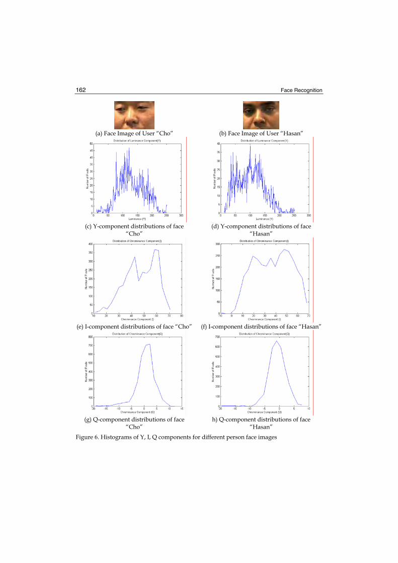
Face Recognition 162
(a) Face Image of User “Cho” (b) Face Image of User “Hasan”
(c) Y-component distributions of face “Cho”
(d) Y-component distributions of face “Hasan”
(e) I-component distributions of face “Cho” (f) I-component distributions of face “Hasan”
(g) Q-component distributions of face “Cho”
h) Q-component distributions of face “Hasan”
Figure 6. Histograms of Y, I, Q components for different person face images
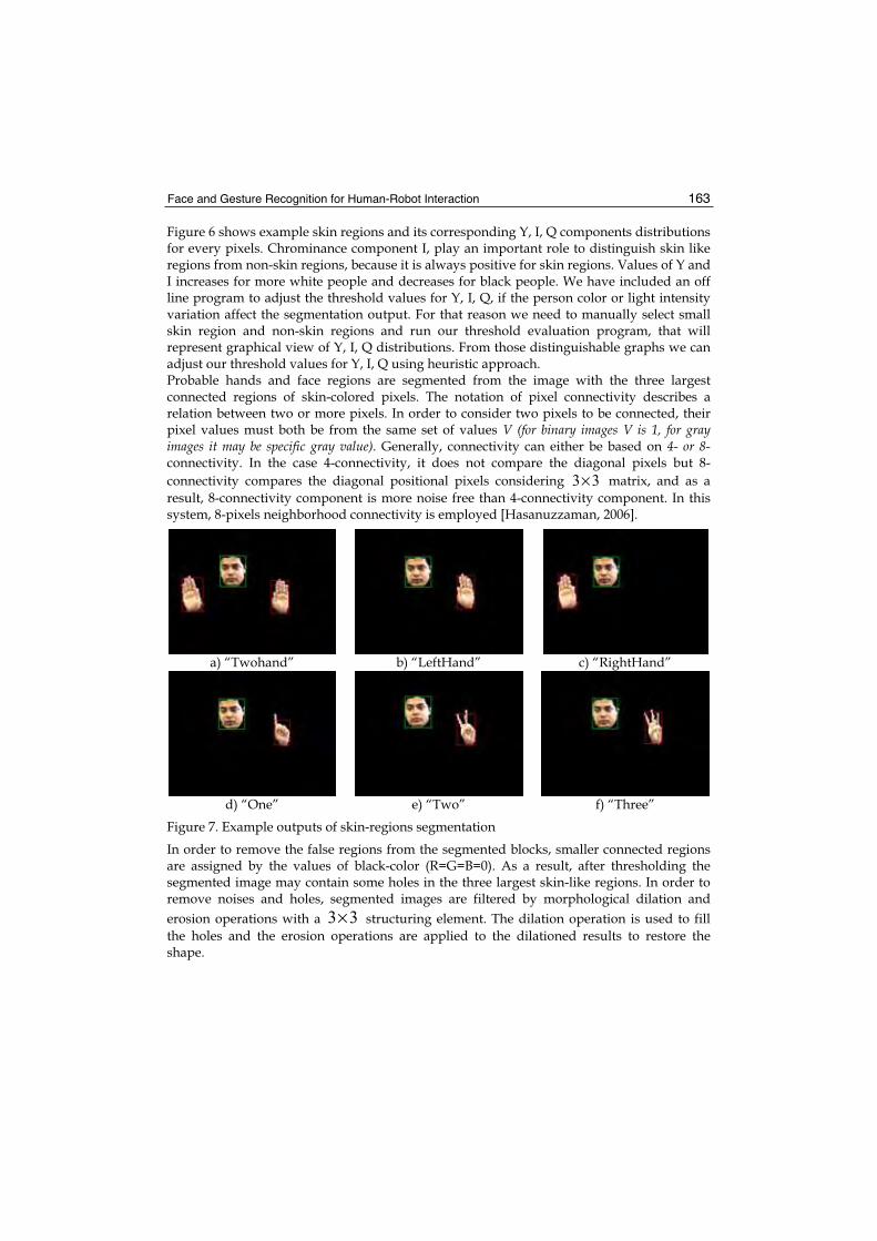
Face and Gesture Recognition for Human-Robot Interaction 163
Figure 6 shows example skin regions and its corresponding Y, I, Q components distributions for every pixels. Chrominance component I, play an important role to distinguish skin like regions from non-skin regions, because it is always positive for skin regions. Values of Y and I increases for more white people and decreases for black people. We have included an off line program to adjust the threshold values for Y, I, Q, if the person color or light intensity variation affect the segmentation output. For that reason we need to manually select small skin region and non-skin regions and run our threshold evaluation program, that will represent graphical view of Y, I, Q distributions. From those distinguishable graphs we can adjust our threshold values for Y, I, Q using heuristic approach. Probable hands and face regions are segmented from the image with the three largest connected regions of skin-colored pixels. The notation of pixel connectivity describes a relation between two or more pixels. In order to consider two pixels to be connected, their pixel values must both be from the same set of values V (for binary images V is 1, for gray images it may be specific gray value). Generally, connectivity can either be based on 4- or 8-connectivity. In the case 4-connectivity, it does not compare the diagonal pixels but 8-connectivity compares the diagonal positional pixels considering 3 3× matrix, and as a result, 8-connectivity component is more noise free than 4-connectivity component. In this system, 8-pixels neighborhood connectivity is employed [Hasanuzzaman, 2006].
a) “Twohand” b) “LeftHand” c) “RightHand”
d) “One” e) “Two” f) “Three”
Figure 7. Example outputs of skin-regions segmentation
In order to remove the false regions from the segmented blocks, smaller connected regions are assigned by the values of black-color (R=G=B=0). As a result, after thresholding the segmented image may contain some holes in the three largest skin-like regions. In order to remove noises and holes, segmented images are filtered by morphological dilation and erosion operations with a 3 3× structuring element. The dilation operation is used to fill the holes and the erosion operations are applied to the dilationed results to restore the shape.

Face Recognition 164
After filtering, the segmented skin regions are bounded by rectangular box using height and width information of each segment:
1 1( )M N× ,2 2( )M N× , and
3 3( )M N× . Figure 7 shows the example outputs of skin like region segmentation method with restricted background. If the user shirt’s color is similar to skin color then segmentation accuracy is very poor. If the user wears short sleeves or T-shirt then it needs to separate hand palm from arm. This system assumes the person wearing full shirt with non-skin color.
3.2 Normalization
Normalization is done to scale the image to match with the size of the training image and convert the scaled image to gray image [Hasanuzzaman, 2004a]. Segmented images are bounded by rectangular boxes using height and width information of each segment:
1 1( )M N× ,2 2( )M N× , and
3 3( )M N× . Each segment is scaled to be square
images with (60 60)× and converted it to as gray images (BMP image). Suppose, we have a
segment of rectangle [( , ) ( , )]l l h hP x y x y− we sample it to rectangle [(0,0) (60 60)]Q − ×using following expression,
( ) ( )( , ) ( , )
60 60
h l h lq qq ql lx x y yQ P x yy yx x− −= + + (3)
Each segment is converted as gray image (BMP image) and compared with template/training images to find the best match. Using the same segmentation and normalization methods training images and test images are prepared, that is why result of this matching approach is better than others who used different training/template image databases. Beside this, we have included training/template images creation functions in this system so that it can adapt with person and illumination changes. Figure 8 shows the examples of training images for five face poses and ten hand poses.
Figure 8. Examples of training images

Face and Gesture Recognition for Human-Robot Interaction 165
4. Face and Hand Pose Classification by Subspace method
Three larger skin like regions are segmented from the input images considering that two hands and one face may present in the input image frame at a specific time. Segmented areas are filtered, normalized and then compared with the training images for finding the best matches using pattern-matching method. Principal component analysis (PCA) method is a standard pattern recognition approach and many researchers use it for face and hand pose classification [Hasanuzzaman, 2004d]. The main idea of the principal component analysis (PCA) method is to find the vectors that best account for the distribution of target images within the entire image space. In the general PCA method, eigenvectors are calculated from training images that include all the poses or classes. But for classification a large number of hand poses for a large number of users, need large number of training datasets from which eigenvectors generation is tedious and may not be feasible for a personal computer. Considering these difficulties we have proposed pose-specific subspace method that partition the comparison area based on each pose. In pose-specific subspace method, training images are grouped based on pose and eigenvectors for each pose are generated separately. In this method one PCA is used for each pose [Hasanuzzaman, 2005b] [Hasanuzzaman, 2004c]. In the following subsection we have described the algorithm of pose-specific subspace method for face and hand pose classification, which is very similar to general PCA based algorithm.
Symbols Meanings
)(ijT Training images for ith class
)(imu mth Eigenvectors for ith class
)(ilΩ Weight vector for ith class
)(ikω Element of weight vector for ith class
iΦ Average image for ith class
)(ils lth Known image for ith class
ε Euclidean distance among weight vectors
)(ilε Element of Euclidean distance among weight vectors for ith class
Table 1. List of symbols used in subspace method Pose-Specific Subspace Method Subspace method offers an economical representation and very fast classification for vectors with a high number of components. Only the statistically most relevant features of a class are retained in the subspace representation. The subspace method is based on the extraction of the most conspicuous properties of each class separately as represented by a set of prototype sample. The main idea of the subspace method is similar to principal component

Face Recognition 166
analysis, is to find the vectors that best account for the distribution of target images within the entire image space. In subspace method target image is projected on each subspace separately. Table 1 summarizes the symbols that are used for describing pose-specific subspace method for face and hand poses classification. The procedure of face and hand pose classification using pose-specific subspace method includes following operations: (I) Prepare noise free version of predefined face and hand poses to form training images
( ) ( )ijT N N× , where j is number training images of ith class (each pose represent one class)
and j=1,2,…., M. Figure 8 shows the example training image classes: frontal face, right directed face, left directed face, up directed face, down directed face, left hand palm, right hand palm, raised index finger, raised index and middle finger to form “V” sign, raised index, middle and ring fingers, fist up, make circle using thumb and fore fingers, thumb up, point left by index finger and point right by index finger are defined as pose P1, P2, P3, P4, P5, P6, P7, P8, P9, P10, P11, P12, P13, P14 and P15 respectively.
(II) For each class, calculate eigenvectors ( )( )imu using Matthew Turk and Alex Pentland
technique [Turk, 1991] and chose k-number of eigenvectors ( )( )iku corresponding to the highest eigenvalues to form principal components for that class. These vectors for each class define the subspace of that pose [for detail please refer to Appendix B]. (III) Calculate corresponding distribution in k-dimensional weight space for the known training images by projecting them onto the subspaces (eigenspaces) of the corresponding class and determine the weight vectors ( )( )ilΩ , using equations (4) and (5).
( ) ( ) ( )( ) ( )i i T i
k l ik u sω = −Φ (4)
( )
1
( ) ( ) ( )
2[ , ,..., ]ii i i
l kω ω ωΩ = (5)
Where, average image of ith class 1
1i n
MT
M nΦ =
=and ( ) ( )i
ls N N× is lth known images of ith
class. (IV) Each segmented skin-region is treated as individual test input image, transformed into eigenimage components and calculated a set of weight vectors ( (i)) by projecting the input image onto each of the subspace as equations (4) and (5). (V) Determine if the image is a face pose or other predefined hand pose based on minimum Euclidean distance among weight vectors using equation (6) and (7),
( ) ( ) ( )|| ||i i il lε = Ω −Ω (6)
( )arg min{ }ijε ε= (7)
If ε is lower than predefined threshold then its corresponding pose is identified. For exact matching ε should be zero but for practical purposes this method uses a threshold value obtained from experiment. If the pose is identified then corresponding pose frame will be activated.

Face and Gesture Recognition for Human-Robot Interaction 167
5. Face and Gesture Recognition
A number of techniques have been developed to detect and recognize face and gesture. For secure or operator specific gesture-based human machine interaction, user identification or face recognition is important. The meaning of the gesture may differ from person to person based on their culture. Suppose according to his culture, user “Hasan” uses “ThumbUp” gesture to terminate an action of robot, whereas user “Cho” uses this gesture to repeat the previous action. In order to person specific gesture interpret (i.e., gesture is same but different meaning for different users) or person dependent gesture command generation we should map user, gesture and robot action.
5.1 Face Recognition
Face recognition is important for human-robot natural interaction and person dependent gesture command generation, i.e, gesture is same but different meaning for different persons. If any segment (skin-like region) is classified as a face, then it needs to classify the pattern, whether it belongs to a known person or not. The detected face is filtered in order to remove noises and normalized so that it matches with the size and type of the training image. The detected face is scaled to be a square image with 60 60× dimension and converted to be a gray image. This face pattern is classified using the eigenface method [Turk, 1991], whether it belongs to known person or unknown person. The face recognition method uses five face classes: frontal face (P1), right directed face (P2), left directed face (P3), up state face (P4) and down state face (P5) in training images as shown in Figure 8 (top row). The eigenvectors are calculated from the known persons face images for each face class and k-number of eigenvectors corresponding to the highest eigenvalues are chosen to form principal components for each class. For each class we have formed subspaces and projected known person face images and detected face image on those subspaces using equation (4) and (5). We get weight vectors for known person images and detected face images. The Euclidean distance is determined between the weight vectors generated from the training images and the weight vectors generated from the detected face by projecting them onto the eigenspaces using equation (6) and (7). If minimum Euclidian distance is lower than the predefined threshold then corresponding person is identified other wise result is unknown person [Hasanuzzaman, 2004c]. We have used face recognition output for human robot (‘Robovie’) greeting application. For example, if the person is known then robot say (“ Hi, person name,How are you?”) but for unknown person robot say (“I do not know you”). We found that the accuracy of frontal face recognition is better than up, down and more left right directed faces [Hasanuzzaman, 2004c]. In this person identification system we prefer frontal and a small left or right rotated faces. Figure 9 shows the sample outputs of face detection method. We have verified this face recognition method for 680 faces of 7 persons, where two are females. Table 2 shows the confusion matrix for the results of face recognition for 7-persons. The diagonal elements represent the correct recognition of corresponding persons. In this table, the 1st column represents the input image classes and other columns represent the recognition results. For example, among 136 face images of person “Hasan”, 132 are correctly recognized as “Hasan” and 4 are wrongly recognized as another person “Vuthi”.
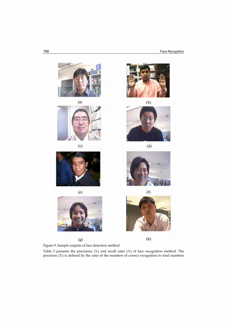
Face Recognition 168
Figure 9. Sample outputs of face detection method
Table 3 presents the precisions (%) and recall rates (%) of face recognition method. The precision (%) is defined by the ratio of the numbers of correct recognition to total numbers

Face and Gesture Recognition for Human-Robot Interaction 169
of recognition for each person faces. The recall rate (%) is defined by the ratio of the numbers of correct face recognition to total numbers of input faces for each person. In the case of person “Pattra” (Figure 9(d)), the precision of face recognition is very low because his face has one black spot.
Input Hasan Ishida Pattara Somjai Tuang Vuthi Cho Hasan(136) 132 0 0 0 0 4 0
Ishida(41) 0 41 0 0 0 0 0
Pattara(41) 0 0 38 3 0 0 0
Somjai(126) 0 0 5 118 3 0 0
Tuang(76) 0 0 0 10 66 0 0
Vuthi(103) 0 0 7 0 5 91 0
Cho(157) 0 0 0 0 0 0 157
Table 2. Confusion Matrix of face recognition
Person Precision (%) Recall (%) Hasan 100% 97.05% Ishida 100% 100%
Pattara 76% 92.68%
Somjai 90.07% 93.65% Tuang 89.18% 86.84% Vuthi 95.78% 88.34%
Cho 100% 100%
Table 3. Performance evaluation of face recognition method
5.2 Gesture Recognition
Gesture recognition is the process by which gestures made by the user are known to the system. Gesture components are the face and hand poses. Gestures are recognized using rule-based system according to predefined model with the combinations of the pose classification results of three segments at a particular image frame. For examples, if left hand palm, right hand palm and one face present in the input image then recognizes it as “TwoHand” gesture and corresponding gesture command generated. If one face and left hand open palm are present in the input image frame then recognized it as “LeftHand” gesture. Similarly others static gestures as listed in Table 4 are recognized. It is possible to recognize more gesture including new poses and new rules using this system. According to recognized gestures, corresponding gesture commands are generated and sent to interact with robot through TCP-IP network.
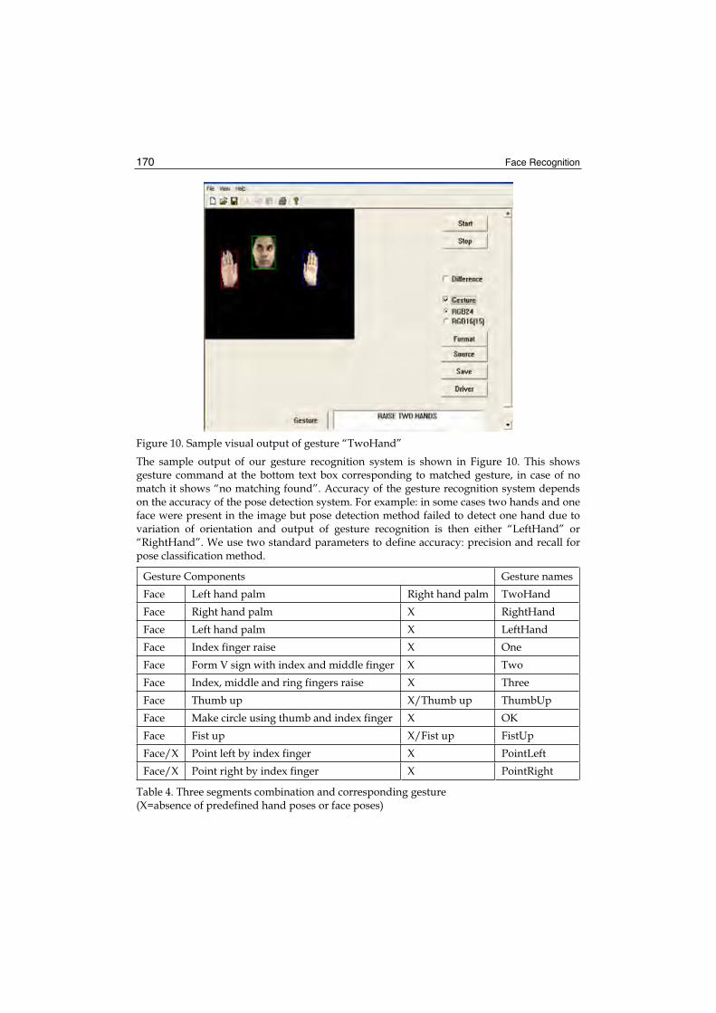
Face Recognition 170
Figure 10. Sample visual output of gesture “TwoHand”
The sample output of our gesture recognition system is shown in Figure 10. This shows gesture command at the bottom text box corresponding to matched gesture, in case of no match it shows “no matching found”. Accuracy of the gesture recognition system depends on the accuracy of the pose detection system. For example: in some cases two hands and one face were present in the image but pose detection method failed to detect one hand due to variation of orientation and output of gesture recognition is then either “LeftHand” or “RightHand”. We use two standard parameters to define accuracy: precision and recall for pose classification method.
Gesture Components Gesture names Face Left hand palm Right hand palm TwoHand Face Right hand palm X RightHand Face Left hand palm X LeftHand Face Index finger raise X One Face Form V sign with index and middle finger X Two Face Index, middle and ring fingers raise X Three Face Thumb up X/Thumb up ThumbUp Face Make circle using thumb and index finger X OK Face Fist up X/Fist up FistUp Face/X Point left by index finger X PointLeft Face/X Point right by index finger X PointRight
Table 4. Three segments combination and corresponding gesture (X=absence of predefined hand poses or face poses)
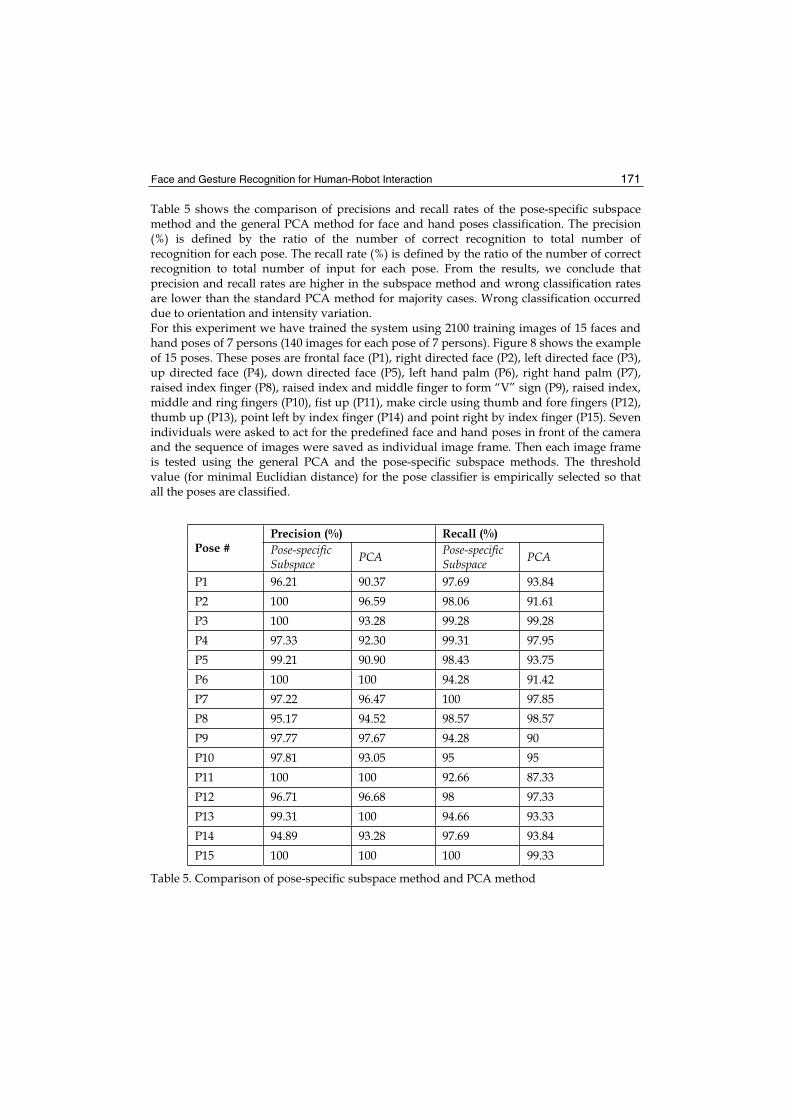
Face and Gesture Recognition for Human-Robot Interaction 171
Table 5 shows the comparison of precisions and recall rates of the pose-specific subspace method and the general PCA method for face and hand poses classification. The precision (%) is defined by the ratio of the number of correct recognition to total number of recognition for each pose. The recall rate (%) is defined by the ratio of the number of correct recognition to total number of input for each pose. From the results, we conclude that precision and recall rates are higher in the subspace method and wrong classification rates are lower than the standard PCA method for majority cases. Wrong classification occurred due to orientation and intensity variation. For this experiment we have trained the system using 2100 training images of 15 faces and hand poses of 7 persons (140 images for each pose of 7 persons). Figure 8 shows the example of 15 poses. These poses are frontal face (P1), right directed face (P2), left directed face (P3), up directed face (P4), down directed face (P5), left hand palm (P6), right hand palm (P7), raised index finger (P8), raised index and middle finger to form “V” sign (P9), raised index, middle and ring fingers (P10), fist up (P11), make circle using thumb and fore fingers (P12), thumb up (P13), point left by index finger (P14) and point right by index finger (P15). Seven individuals were asked to act for the predefined face and hand poses in front of the camera and the sequence of images were saved as individual image frame. Then each image frame is tested using the general PCA and the pose-specific subspace methods. The threshold value (for minimal Euclidian distance) for the pose classifier is empirically selected so that all the poses are classified.
Precision (%) Recall (%) Pose # Pose-specific
Subspace PCA Pose-specificSubspace PCA
P1 96.21 90.37 97.69 93.84 P2 100 96.59 98.06 91.61 P3 100 93.28 99.28 99.28 P4 97.33 92.30 99.31 97.95 P5 99.21 90.90 98.43 93.75 P6 100 100 94.28 91.42 P7 97.22 96.47 100 97.85 P8 95.17 94.52 98.57 98.57 P9 97.77 97.67 94.28 90 P10 97.81 93.05 95 95 P11 100 100 92.66 87.33 P12 96.71 96.68 98 97.33 P13 99.31 100 94.66 93.33 P14 94.89 93.28 97.69 93.84 P15 100 100 100 99.33
Table 5. Comparison of pose-specific subspace method and PCA method

Face Recognition 172
6. Implementation Scenarios
Our approach has been verified using a humanoid robot ‘Robovie’ and an entertainment robot ‘Aibo’. This section describes example scenarios, which integrates gestures commands and corresponding robot behaviors. For interaction with an ‘Aibo’ robot, a standard CCD video camera is attached to the computer (Image analysis and recognition PC) to capture the real-time images. In the case of ‘Robovie’ robot, its eyes cameras are used for capturing the real time images. Each captured image is digitized into a matrix of 320 240× pixels with 24-bit color. First, the system is trained using the known training images of predefined faces and hand poses of all known persons. All the training images are 60 60× pixels gray images. In the training phase, this system generates eigenvectors and feature vectors for the known users and hand poses. We have considered robot as a server and our PC as a client. Communication link has been established through TCP-IP protocol. Initially, we connected the client PC with robot server and then gestures recognition program was run in the client PC. The result of gesture recognition program generates gesture commands and sends to robot. After getting gesture command robot acted according to user predefined actions. We have considered for human-robot interaction that gesture command will be effective until robot finishes corresponding action for that gesture.
Figure 11. Human robot (‘Robovie’) interaction scenario
6.1 Example of Interaction with Robovie
Figure 11 shows the example of human interaction with a ‘Robovie’ robot [Hasanuzzaman, 2005b]. The user steps in front of the eyes camera and raises his two hands. The image analysis and recognition module recognizes the user as ‘Hasan’ and classifies the three poses as ‘FACE’, ‘LEFTHAND’, ‘RIGHTHAND’. This module sends gesture command

Face and Gesture Recognition for Human-Robot Interaction 173
according to gesture name and user name, and selected robot function will be activated. This system implements person-centric gesture-based human robot interaction. The same gesture can be used to activate different actions for different persons even the robot is same. The robot actions are mapped based on the gesture user relationships (“gesture-user-robot-action”) in the knowledge base. In this case, “Robovie” raises its two arms (as shown in Figure 11) and says “Raise Two Arms”. This system has considered that gesture command will be effective until the robot finishes corresponding action for that gesture. This method has been implemented on a ‘Robovie’ for the following scenarios:
User: “Hasan” comes in front of Robovie eyes camera, and the robot recognizes the user as Hasan.
Robot: “Hi Hasan, How are you?” (Speech)
Hasan: uses the gesture “ThumbUp”
Robot: “ Oh, sad, do you want to play now?” (Speech)
Hasan: uses the gesture “Ok”,
Robot: “Thanks!” (Speech)
Hasan: uses the gesture “TwoHand”
Robot: imitate user’s gesture “Raise Two Arms” as shown in Figure6.
Hasan: uses the gesture “FistUp” (stop the action)
Robot: Bye-bye (Speech).
User: “Cho” comes in front of Robovie eyes camera and robot recognizes the user as Cho.
Robot: “Hi Cho, How are you?” (Speech)
Cho: uses the gesture “ThumbUp”.
Robot: “ Oh, good, do you want to play now?” (Speech)
Cho: uses the gesture “Ok”.
Robot: “Thanks!” (Speech)
Cho: uses the gesture “LeftHand”
Robot: imitate user’s gesture (“Raise Left Arm”).
Cho: uses the gesture “TwoHand” (STOP)
Robot: Bye-bye (Speech)
The above scenarios show that same gesture is used for different meanings and several gestures are used for the same meanings for different persons. The user can design new actions according to his/her desires using ‘Robovie’.
6.2 Example of Interaction with Aibo
Figure 12 shows an example of human robot (‘Aibo’) interaction scenario. The system uses a standard CCD video camera for data acquisition. The user raises his index finger in front of the camera that is connected to gesture recognition PC. The image analysis and recognition module classifies the poses “FACE” and “ONE” (hand pose) and corresponding pose frames will be activated. Gestures are interpreted using three components. According to the predefined combination gesture is recognized as “One” and corresponding gesture frame is activated. The gesture recognition module recognizes the gesture is “One” and the face recognition module identifies the person as “Hasan”. The user selects ‘Aibo’ robot for the interaction. In this combination activates the ‘Aibo’ for playing action ‘STAND UP’.
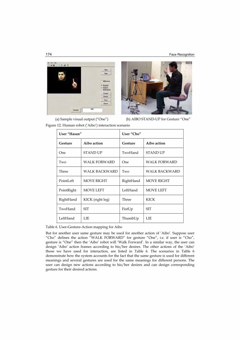
Face Recognition 174
(a) Sample visual output (“One”) (b) AIBO STAND-UP for Gesture “One”
Figure 12. Human robot (‘Aibo’) interaction scenario
User “Hasan” User “Cho”
Gesture Aibo action Gesture Aibo action
One STAND UP TwoHand STAND UP
Two WALK FORWARD One WALK FORWARD
Three WALK BACKWARD Two WALK BACKWARD
PointLeft MOVE RIGHT RightHand MOVE RIGHT
PointRight MOVE LEFT LeftHand MOVE LEFT
RightHand KICK (right leg) Three KICK
TwoHand SIT FistUp SIT
LeftHand LIE ThumbUp LIE
Table 6. User-Gesture-Action mapping for Aibo
But for another user same gesture may be used for another action of ‘Aibo’. Suppose user “Cho” defines the action “WALK FORWARD” for gesture “One”, i.e. if user is “Cho”, gesture is “One” then the ‘Aibo’ robot will ‘Walk Forward’. In a similar way, the user can design ‘Aibo’ action frames according to his/her desires. The other actions of the ‘Aibo’ those we have used for interaction, are listed in Table 6. The scenarios in Table 6 demonstrate how the system accounts for the fact that the same gesture is used for different meanings and several gestures are used for the same meanings for different persons. The user can design new actions according to his/her desires and can design corresponding gesture for their desired actions.

Face and Gesture Recognition for Human-Robot Interaction 175
7. Conclusions and future research
This chapter describes a real-time face and hand gesture recognition system using skin color segmentation and subspace method based pattern matching technique. This chapter also describes gesture-based human-robot interaction system using an entertainment robot named ‘Aibo’ and humanoid robot ‘Robovie’. In pose-specific subspace method, training images are grouped based on pose and eigenvectors for each pose are generated separately. In this method, one PCA is used for each pose. From the experimental result we have concluded that performance of pose-specific subspace method is better than general PCA method in the same environment. One of the major constrains of this system is that the background should be non-skin color substrate. If we used infrared camera then it is possible to overcome this problem just by a minor modification of our segmentation technique and other module will remain the same. Since the skin reflects near IR light nicely, active IR sources placed in proximity to the camera in combination with IR pass filter on the lens makes it easy to locate hands those are within the range of light sources. Considering the reduction of processing time, so far eigenvectors calculations are performed separately in off-line. The eigenvectors do not change during dynamic learning process. The user has to initiate this calculation function to change the eigenvectors or principal components. In future, if faster CPUs are available, these components are then possible to be integrated into on-line learning function. We could not claim that our system is more robust against new lighting condition and clutter background. Our hope is to make this face and gesture recognition system more robust and capable to recognize dynamic facial and hand gesture. Face and gesture recognition simultaneously will help us in future to develop person specific and secure human-robot interface. The ultimate goal of this research is to establish a symbiotic society for all of the distributed autonomous intelligent components so that they share their resources and work cooperatively with human beings.
8. Appendix
8.1 Appendix A: CONVERSION FROM RGB COLOR SPACE TO YIQ COLOR SPACE
This system uses skin-color based segmentation method for determining the probable face and hands areas in an image. There are several color coordinate systems, which have come into existence for a variety of reasons. The YIQ is a universal color space used by NTSC to transmit color images using the existing monochrome television channels without increasing the bandwidth requirements. In the YIQ color model a color is described by three attributes: luminance, hue and saturation. The capture color image is represented by the RGB color coordinate system at each pixel. The colors from RGB space are converted into the YIQ space. The YIQ produces a linear transform of RGB images, which generates Y representing luminance channel and I, Q representing two chrominance channels to carry color information. The transformation matrix for the conversion from RGB to YIQ is given below [Jain, 1995],
0.299 0.587 0.114
0.596 0.274 0.322
0.211 0.523 0.312
Y RI GQ B
= − −−

Face Recognition 176
Where R, G, and B are the red, green, and blue component values which exist in the range [0, 255]. Using the following equations we can converts the images from RGB color coordinates system to YIQ color coordinate system,
0.299 0.587 0.114Y R G B= + + (A.1)
0.596 0.274 0.322I R G B= − − (A.2)
0.211 0.523 0.312Q R G B= − + (A.3)
Images are being searched in YIQ space depending on the amount of color content of these dominant colors, that is, whether the skin color value is substantially present in an image or not. In order to segment face and hand poses in an image, the skin pixels are thresholded empirically. In this experiment, the ranges of threshold values are defined from the Y, I, Q histograms calculated for a selected skin region.
8.2 Appendix B: EIGENVECTORS CALCULATION
This section describes Eigenvectors calculation method from the training images. The major steps of the Eigenvectors calculation algorithm [Smith, 2002] [Turk, 1991] are, Step1: Read all the training images ( )iT N N× those are two-dimensional N by N gray images, where i=1,2, …., M.Step2: Convert each image into a column vector
2( ) ( )i iT N T N N= × (B.1)
Step3: Calculate the mean of all images
1
1
MTiM i
Ψ ==
(B.2)
Step4: Subtract the mean and form a big matrix with all the subtracted image data
i iTφ = −Ψ (B.3)
1 2 3[ , , ,......., ]MA φ φ φ φ= (B.4)
Step5: Calculate the Covariance of matrix ‘A’
TC AA= (B.5)
Step6: Calculate the Eigenvectors and Eigenvalues of the Covariance Matrix
k k ku Cuλ = (B.6)
Where, the vectors ku (non-zero) and scalar kλ are the Eigenvectors and Eigenvalues, respectively, of the Covariance matrix C. The relation between Eigenvectors and Eigenvalues of a Covariance matrix can be written using equation (B.7)

Face and Gesture Recognition for Human-Robot Interaction 177
2
1
1( )
MT
k k nn
uM
λ φ=
= (B.7)
Using MALAB function Eigenvectors and Eigenvalues can be calculated,
[ , ] ( )eigvec eigvalue eig C= (B.8)
Each Eigenvector is of length 2,N describe an N-by-N images and is a linear combination of the original image. Eigenvalues are the coefficient of Eigenvectors. The Eigenvectors are sorted based on Eigenvalues (higher to lower). According higher order of Eigenvalues k-numbers of Eigenvectors are chosen to form principal components.
9. References
L. Aryananda, Recognizing and Remembering Individuals: Online and Unsupervised Face Recognition for Humanoid Robot in Proceeding of IEEE/RSJ International Conference on Intelligent Robots and Systems (IROS 2002), Vol. 2, pp. 1202-1207, 2002. [Aryananda, 2002]
H. Asoh, S. Hayamizu, I. Hara, Y. Motomura, S. Akaho and T. Matsui, Socially Embedded Learning of the Office-Conversant Mobile Robot Iijo-2, in Proceeding of 15th International Joint-Conference on Artificial Intelligence (IJCAI’97), pp.880-885, 1997. [Asoh, 1997]
M. F. Augusteijn, and T.L. Skujca, Identification of Human Faces Through Texture-Based Feature Recognition and Neural Network Technology, in Proceeding of IEEE conference on Neural Networks, pp.392-398, 1993. [Augusteijn, 1993]
R. E. Axtell, Gestures: The Do’s and Taboos of Hosting International Visitors, John Wiley & Sons, 1990. [Axtell, 1990]
Y. Azoz, L. Devi, and R. Sharma, Reliable Tracking of Human Arm Dynamics by Multiple Cue Integration and Constraint Fusion, in Proceeding of IEEE Computer Society Conference on Computer Vision and Pattern Recognition (CVPR’98), pp. 905-910, 1998. [Azoz, 1998]
D. H. Ballard, Christopher M. Brown, Computer Vision, Prentic-Hall, INC., New Jersey, USA, 1982. [Ballard, 1982]
M. S Bartlett, H. M. Lades, and, T. Sejnowski, Independent Component Representation for Face Recognition in Proceedings of Symposium on Electronic Imaging (SPEI): Science and Technology, pp. 528-539, 1998. [Bartlett, 1998]
C. Bartneck, M. Okada, Robotic User Interface, in Proceeding of Human and Computer Conference (Hc-2001), Aizu, pp. 130-140, 2001. [Bartneck, 2001]
P.N. Belhumeur, J. P. Hespanha, and D. J. Kriegman, Eigenfaces vs. Fisherfaces: Recognition Using Class Specific Linear Projection IEEE Transaction on Pattern Analysis and Machine Intelligence (PAMI), Vol. 19, pp. 711-720, 1997. [Belhumeur, 1997]
M. A. Bhuiyan, V. Ampornaramveth, S. Muto, and H. Ueno, On Tracking of Eye For Human-Robot Interface, International Journal of Robotics and Automation, Vol. 19, No. 1, pp. 42-54, 2004. [Bhuiyan, 2004]

Face Recognition 178
M. A. Bhuiyan, V. Ampornaramveth, S. Muto, H. Ueno, Face Detection and Facial Feature Localization for Human-machine Interface, NII Journal, Vol.5, No. 1, pp. 25-39, 2003. [Bhuiyan, 2003]
M. Billinghurst, Chapter 14: Gesture-based Interaction, Human Input to Computer Systems: Theories, Techniques and Technologies, (ed. By W. Buxton), 2002. [Billinghurst, 2002]
L. Brethes, P. Menezes, F. Lerasle and J. Hayet, Face Tracking and Hand Gesture Recognition for Human-Robot Interaction, in Proceeding of International Conference on Robotics and Automation (ICRA 2004), pp. 1901-1906, 2004. [Brethes, 2004]
H. Birk, T. B. Moeslund, and C. B. Madsen, Real-time Recognition of Hand Alphabet Gesture Using Principal Component Analysis, in Proceeding of 10th Scandinavian Conference on Image Analysis, Finland, 1997. [Birk, 1997]
R. Chellappa, C. L. Wilson, and S. Sirohey, Human and Machine Recognition of faces: A survey, in Proceeding of IEEE, Vol. 83, No. 5, pp. 705-740, 1995. [Chellappa, 1995]
D. Chetverikov and A. Lerch, Multiresolution Face Detection, Theoretical Foundation of Computer Vision, Vol. 69, pp. 131-140, 1993. [Chetverikov, 1993]
K. Chung, S. C. Kee, and S. R. Kim, Face Recognition using Principal Component Analysis of Gabor Filter Reponses, in Proceedings of International Workshop on Recognition, Analysis and Tracking of Faces and Gestures in Real-time Systems, pp. 53-57, 1999. [Chung, 1999]
C. J. Cohen, G. Beach, G. Foulk, A Basic Hand Gesture Control System for PC Applications, in Proceedings of Applied Imagery Pattern Recognition Workshop (AIPR’01), pp. 74-79, 2001. [Cohen, 2001]
J. L. Crowley and F. Berard, Multi Modal Tracking of Faces for Video Communications, In Proceedings of IEEE Conference on Computer Vision and Pattern Recognition (CVPR’97), pp. 640-645, 1997. [Crowley, 1997]
R. Cutler, M. Turk, View-based Interpretation of Real-time Optical Flow for Gesture Recognition, in Proceedings of 3rd International Conference on Automatic Face and Gesture Recognition (AFGR’98), pp. 416-421, 1998. [Cutler, 1998]
Y. Dai and Y. Nakano, Face-Texture Model Based on SGLD and Its Application in Face Detection in a Color Scene, Pattern Recognition, Vol. 29, No. 6, pp.1007-1017, 1996. [Dai, 1996]
T. Darrel, G. Gordon, M. Harville and J. J Woodfill, Integrated Person Tracking Using Stereo, Color, and Pattern Detection, International Journal of Computer Vision, Vol. 37, No. 2, pp. 175-185, 2000. [Darrel, 2000]
T. Darrel and A. Pentland, Space-time Gestures, in Proceedings of IEEE International Conference on Computer Vision and Pattern recognition (CVPR’93), pp. 335-340, 1993. [Darrel, 1993]
J. W. Davis, Hierarchical Motion History Images for Recognizing Human Motion, in Proceeding of IEEE Workshop on Detection and Recognition of Events in Video(EVENT’01), pp.39-46, 2001. [Davis, 2001]
S. S. Fels, and G. E. Hinton, Glove-Talk: A neural Network Interface Between a Data-Glove and Speech Synthesizer, IEEE Transactions on Neural Networks, Vol. 4, pp. 2-8, 1993. [Fels, 1993]
The Festival Speech Synthesis System developed by CSTR, University of Edinburgh, http://www.cstr.ed.ac.uk/project/festival. [Festival, 1999]

Face and Gesture Recognition for Human-Robot Interaction 179
T. Fong, I. Nourbakhsh and K. Dautenhahn, A Survey of Socially Interactive Robots, Robotics and Autonomous System, Vol. 42(3-4), pp.143-166, 2003. [Fong, 2003]
W.T. Freeman, K. Tanaka, J. Ohta, and K. Kyuma, Computer Vision for Computer Games, in Proceedings of International Conference on Automatic Face and Gesture Recognition(AFGR’96), pp. 100-105, 1996. [Freeman, 1996]
M. Hasanuzzaman, T. Zhang, V. Ampornaramveth, and H. Ueno: Gesture-Based Human-Robot Interaction Using a Knowledge-Based Software Platform, International Journal of Industrial Robot, Vol. 33(1), 2006. [Hasanuzzaman, 2005a]
M. Hasanuzzaman, T. Zhang, V. Ampornaramveth, H. Gotoda, Y. Shirai, and H. Ueno, Knowledge-Based Person-Centric Human-Robot Interaction by Means of Gestures, International Journal of Information Technology, Vol. 4(4), pp. 496-507, 2005. [Hasanuzzaman, 2005b]
M. Hasanuzzaman, V. Ampornaramveth, T. Zhang, M. A. Bhuiyan, Y. Shirai, H. Ueno, Real-time Vision-based Gesture Recognition for Human-Robot Interaction, in Proceeding of IEEE International Conference on Robotics and Biomimetics (ROBIO’2004), China, pp. 379-384, 2004. [Hasanuzzaman, 2004a]
M. Hasanuzzaman, T. Zhang, V. Ampornaramveth, M.A. Bhuiyan, Y. Shirai, H. Ueno, Gesture Recognition for Human-Robot Interaction Through a Knowledge Based Software Platform, in Proceeding of IEEE International Conference on Image Analysis and Recognition (ICIAR 2004), LNCS 3211 (Springer-Verlag Berlin Heidelberg), Vol. 1, pp. 5300-537, Portugal, 2004. [Hasanuzzaman, 2004b]
M. Hasanuzzaman, V. Ampornaramveth, T. Zhang, M.A. Bhuiyan, Y. Shirai, H. Ueno, Face and Gesture Recognition Using Subspace Method for Human-Robot Interaction, Advances in Multimedia Information Processing - PCM 2004: in Proceeding of 5th Pacific Rim Conference on Multimedia, LNCS 3331 (Springer-Verlag Berlin Heidelberg) Vol. 1, pp. 369-376, Tokyo, Japan, 2004. [Hasanuzzaman, 2004c]
M. Hasanuzzaman, T. Zhang, V. Ampornaramveth, P. Kiatisevi, Y. Shirai, H. Ueno, Gesture-based Human-Robot Interaction Using a Frame-based Software Platform, in Proceeding of IEEE International Conference on Systems Man and Cybernetics (IEEE SMC’2004), Netherland, 2004. [Hasanuzzaman, 2004d]
[M. Hasanuzzaman, M.A. Bhuiyan, V. Ampornaramveth, T. Zhang, Y. Shirai, H. Ueno, Hand Gesture Interpretation for Human-Robot Interaction, in Proceeding of International Conference on Computer and Information Technology (ICCIT’2004), Bangladesh, pp. 149-154, 2004. Hasanuzzaman, 2004e]
C. Hu, Gesture Recognition for Human-Machine Interface of Robot Teleoperation, in Proceeding of International Conference on Intelligent Robots and Systems, pp. 1560-1565, 2003. [Hu, 2003]
[Huang, 1994] G. Yang, and T. S. Huang, Human Face Detection in Complex Background Pattern Recognition, Vol. 27, No. 1, pp. 53-63, 1994.
Gary Imai Gestures: Body Language and Nonverbal Communication,http://www.csupomona.edu/~tassi/gestures.htm, visited on June 2004. [Imai, 2004]
Robovie, http://www.mic.atr.co.jp/~michita/everyday-e/[Imai, 2000] A. K. Jain, Fundamental of Digital Image Processing, Prentice-Hall of India Private Limited,
New Delhi, 1995. [Jain, 1995]

Face Recognition 180
T. Kanade, Computer Recognition of Human Faces, Brikhauser Verlag, Basel and Stuttgart, ISR-47, pp. 1-106, 1977. [Kanade, 1977]
S. Kawato and J. Ohya, Real-time Detection of Nodding and Head-Shaking by Directly Detecting and Tracking the ‘Between-Eyes’, in Proceeding of IEEE International Conference on Automatic Face and Gesture Recognition (AFGR’2000), pp.40-45, 2000. [Kawato, 2000]
M. D. Kelly, Visual Identification of People by Computer, Technical report, AI-130, Stanford AI projects, Stanford, CA, 1970. [Kelly, 1970]
R. Kjeldsen, and K. Kender, Finding Skin in Color Images, in Proceedings of 2nd International Conference on Automatic Face and Gesture Recognition (AFGR’96), pp. 312-317, 1996. [Kjeldsen, 1996]
C. Kotropoulos and I. Pitas, Rule-based Face Detection in Frontal Views, in Proceeding of International Conference on Acoustics, Speech and Signal Processing, Vol. 4, pp. 2537-2540, 1997. [Kotropoulos, 1997]
J. Kramer, L. Larry Leifer, The Talking Glove: A Speaking Aid for Non-vocal Deaf and Deaf-blind Individuals, in Proceedings of 12th Annual Conference, RESNA (Rehabilitation Engineering & Assistive Technology), pp. 471-472, 1989. [Kramer, 1989]
S. J. Lee, S. B. Jung, J. W. Kwon, S. H. Hong, Face Detection and Recognition Using PCA, in Proceedings of IEEE Region 10th Conference (TENCON’99) pp. 84-87, 1999. [Lee, 1999]
C. Lee, and Y. Xu, Online, Interactive Learning of Gestures for Human/Robot Interfaces, in Proceedings of IEEE International Conference on Robotics and Automation (ICRA’96), Vol. 4, pp. 2982-2987, 1996. [Lee, 1996]
J. Lin, Y. Wu, and T. S Huang, Capturing Human Hand Motion in Image Sequences, in Proceeding of Workshop on Motion and Video Computing, Orlando, Florida, December, 2002. [Lin, 2002]
X. Lu, Image Analysis for Face Recognition-A Brief Survey, Personal notes, pp. 1-37, 2003. [Lu, 2003]
J. Miao, B. Yin, K. Wang, L. Shen, and X. Chen, A Hierarchical Multiscale and Multiangle System for Human Face Detection in a Complex Background Using Gravity-Centre Template, Pattern Recognition, Vol. 32, No. 7, pp. 1237-1248, 1999. [Miao, 1999]
Application Wizard: Microsoft Foundation Class, VideoIn, Microsoft Corp. [Microsoft] B. Moghaddam and A. Pentland, Probabilistic Visual Learning for Object Detection, in
Proceeding of 5th International Conference on Computer Vision, pp. 786-793, 1995. [Moghaddam, 1995]
Y. Nam and K. Y. Wohn, Recognition of Space-Time Hand-Gestures Using Hidden Markov Model, in Proceedings of ACM Symposium on Virtual Reality Software and Technology,pp. 51-58, 1996. [Nam, 1996]
J. L. Nespoulous, P. Perron, and A. Roch Lecours, The Biological Foundations of Gestures: Motor and Semiotic Aspects, Lawrence Erlbaum Associates, Hillsdale, New Jersey, 1986. [Nespoulous, 1986]
R. O’Hagan, Finger Track-A Robust and Real-Time Gesture Interface, in Proceeding of 10th Australian Joint Conference on Artificial Intelligence: Advance Topics in Artificial Intelligence, LNCS, Vol. 1342, pp. 475-484, 1997. [O’Hagan, 1997]
K. Oka, Y. Sato, and H. Koike, Real-Time Tracking of Multiple Finger-trips and Gesture Recognition for Augmented Desk Interface Systems, in Proceeding of International

Face and Gesture Recognition for Human-Robot Interaction 181
Conference in Automatic Face and Gesture Recognition (AFGR’02), pp. 423-428, Washington D.C, USA, 2002. [Oka, 2002]
D. W. Patterson, Introduction to Artificial Intelligence and Expert Systems, Prentice-Hall Inc., Englewood Cliffs, N.J, USA, 1990. [Patterson, 1990]
A. Pentland, B. Moghaddam, and T. Starner, View-based and Modular Eigenspaces for Face Recognition, in Proceeding of IEEE International Conference on Computer Vision and Pattern Recognition (CVPR’94), pp. 84-91, 1994. [Pentland, 1994]
V. I. Pavlovic, R. Sharma and T. S. Huang, Visual Interpretation of Hand Gestures for Human-Computer Interaction: A Review, IEEE Transactions on Pattern Analysis and Machine Intelligence (PAMI), Vol. 19, No. 7, pp. 677-695, 1997. [Pavlovic, 1997]
J. M. Rehg and T. Kanade, Digiteyes: Vision-based Hand Tracking for Human-Computer Interaction, in Proceeding of Workshop on Motion of Non-Rigid and Articulated Bodies,pp. 16-94, 1994. [Rehg, 1994]
G. Rigoll, A. Kosmala, S. Eickeler, High Performance Real-Time Gesture Recognition Using Hidden Markov Models, in Proceeding of International Gesture Workshop on Gesture and Sign Language in Human Computer Interaction, pp. 69-80, Germany, 1997. [Rigoll, 1997]
H. A. Rowley, S. Baluja and T. Kanade, Neural Network-Based Face Detection IEEE Transactions on Pattern Analysis and Machine Intelligence (PAMI), Vol. 23, No. 1, pp. 23-38, 1998. [Rowley, 1998]
E. Saber and A. M. Tekalp, Frontal-view Face Detection and Facial Feature Extraction Using Color, Shape and Symmetry Based Cost Functions, Pattern Recognition Letters, Vol. 17(8) pp.669-680, 1998. [Saber, 1998]
T. Sakai. M. Nagao and S. Fujibayashi, Line Extraction and Pattern Detection in a Photograph, Pattern Recognition, Vol. 1, pp.233-248, 1996. [Sakai, 1996]
N. Shimada, and Y. Shirai, 3-D Hand Pose Estimation and Shape Model Refinement from a Monocular Image Sequence, in Proceedings of VSMM’96 in GIFU, pp.23-428, 1996. [Shimada, 1996]
S. A. Sirohey, Human Face Segmentation and Identification, Technical Report CS-TR-3176, University of Maryland, pp. 1-33, 1993. [Sirohey, 1993]
L. I. Smith, A Tutorial on Principal Components Analysis, February 26, 2002. [Smith, 2002] T. Starner, J. Weaver, and Alex Pentland, Real-time American Sign Language Recognition
Using Desk and Wearable Computer Based Video, IEEE Transactions on Pattern Analysis and Machine Intelligence (PAMI), Vol. 20, No.12, pp. 1371-1375, 1998. [Starner, 1998]
D.J. Sturman and D. Zetler, A Survey of Glove-Based Input, IEEE Computer Graphics and Applications, Vol. 14, pp-30-39, 1994. [Sturman, 1994]
J. Triesch and C. V. Malsburg, Classification of Hand Postures Against Complex Backgrounds Using Elastic Graph Matching, Image and Vision Computing, Vol. 20, pp. 937–943, 2002. [Triesch, 2002]
A. Tsukamoto, C.W. Lee, and S. Tsuji, Detection and Pose Estimation of Human Face with Synthesized Image Models, in Proceeding of International Conference of Pattern Recognition, pp. 754-757,1994. [Tsukamoto, 1994]
C. Torras, Robot Adaptivity, Robotics and Automation Systems, Vol. 15, pp.11-23, 1995. [Torras, 1995]

Face Recognition 182
M. Turk and G. Robertson, Perceptual user Interfaces, Communication of the ACM, Vol. 43, No. 3, pp.32-34, 2000. [Turk, 2000]
M. Turk and A. Pentland, Eigenface for Recognition, Journal of Cognitive Neuroscience, Vol. 3, No.1, pp. 71-86, 1991. [Turk, 1991]
H. Ueno, Symbiotic Information System: Towards an Ideal Relationship of Human Beings and Information Systems, Technical Report of IEICE, KBSE2001-15: pp.27-34, 2001. [Ueno, 2001]
A. Utsumi, N. Tetsutani and S. Igi, Hand Detection and Tracking Using Pixel Value Distribution Model for Multiple-Camera-Based Gesture Interactions, in Proceeding of IEEE Workshop on Knowledge Media Networking (KMN’02), pp. 31-36, 2002. [Utsumi, 2002]
S. Waldherr, R. Romero, S. Thrun, A Gesture Based Interface for Human-Robot Interaction, Journal of Autonomous Robots, Kluwer Academic Publishers, pp. 151-173, 2000. [Waldherr, 2000]
T. Watanabe, M. Yachida, Real-time Gesture Recognition Using Eigenspace from Multi-Input Image Sequences, System and Computers in Japan, Vol. J81-D-II, pp. 810-821, 1998. [Watanabe, 1998]
L. Wiskott, J. M. Fellous, N. Kruger, and C. V. Malsburg, Face Recognition by Elastic Bunch Graph Matching, IEEE Transactions on Pattern Analysis and Machine Intelligence(PAMI), Vol. 19, No.7, pp. 775-779, 1997. [Wiskott, 1997]
M. H. Yang, D. J. Kriegman and N. Ahuja, Detection Faces in Images: A survey, IEEE Transactions on Pattern Analysis and Machine Intelligence (PAMI), Vol. 24, No. 1, pp. 34-58, 2002. [Yang, 2002]
M. H. Yang, Hand Gesture Recognition and Face Detection in Images, Ph.D Thesis,University of Illinois, Urbana-Champaign, 2000. [Yang, 2000]
J. Yang, R. Stiefelhagen, U. Meier and A. Waibel, Visual Tracking for Multimodal Human Computer Interaction, in Proceedings of ACM CHI’98 Human Factors in Computing Systems, pp. 140-147, 1998. [Yang, 1998]
G. Yang and T. S. Huang, Human Face Detection in Complex Background, Pattern Recognition, Vol. 27, No.1, pp.53-63, 1994. [Yang, 1994]
A. Yuille, P. Hallinan and D. Cohen, Feature Extraction from Faces Using Deformable Templates, International Journal of Computer Vision, Vol. 8, No. 2, pp 99-111, 1992. [Yuille, 1992]
W. Zhao, R. Chellappa, P. J. Phillips, and A. Rosenfeld, Face Recognition: A Literature Survey, ACM Computing Surveys, Vol. 35, No. 4, pp. 399-458, 2003. [Zhao, 2003]
T. Zimmerman, J. Lanier, C. Blanchard, S. Bryson, and Y. Harvil, A Hand Gesture Interface Device, in Proceedings of (CHI+GI)’87, pp. 189-192, 1987. [Zimmerman, 1987]

10
Modelling Uncertainty in Representation of Facial Features for Face Recognition
Hiremath P.S., Ajit Danti and Prabhakar C.J. Gulbarga University, Gulbarga; JNN College of Engineering, Shimoga & Kuvempu
University, Shimoga India
1. Introduction
Face is one of the important biometric identifier used for human recognition. The face recognition involves the computation of similarity between face images belonging to the determination of the identity of the face. The accurate recognition of face images is essential for the applications including credit card authentication, passport identification, internet security, criminal databases, biometric cryptosystems etc. Due to the increasing need for the surveillance and security related applications in access control, law enforcement, and information safety due to criminal activities, the research interest in the face recognition has grown considerably in the domain of the pattern recognition and image analysis. A number of approaches for face recognition have been proposed in the literature (Zhao et al. 2000), (Chellappa et al. 1995). Many researchers have addressed face recognition based on geometrical features and template matching (Brunelli and Poggio, 1993). There are several well known face recognition methods such as Eigenfaces (Turk and Pentland 1991), Fisherfaces (Belhumeur et al. 1997), (Kim and Kitter 2005), Laplacianfaces (He et al. 2005). The wavelet based Gabor function provide a favorable trade off between spatial resolution and frequency resolution (Gabor 1946). Gabor wavelets render superior representation for face recognition (Zhang, et al. 2005), (Shan, et al. 2004), (Olugbenga and Yang 2002). In recent survey, various potential problems and challenges in the face detection are explored (Yang, M.H., et al., 2002). Recent face detection methods based on data-driven learning techniques, such as the statistical modeling methods (Moghaddam and Pentland 1997), (Schneiderman, and Kanade, 2000), (Shih and Liu 2004), the statistical learning theory and SVM based methods (Mohan et al., 2001). Schneiderman and Kanade have developed the first algorithm that can reliably detect human faces with out-of-plane rotation and the first algorithm that can reliably detect passenger cars over a wide range of viewpoints (Schneiderman and Kanade 2000). The segmentation of potential face region in a digital image is a prelude to the face detection, since the search for the facial features is confined to the segmented face region. Several approaches have been used so far for the detection of face regions using skin color information. In (Wu, H.Q., et al., 1999), a face is detected using a fuzzy pattern matching method based on skin and hair color. This method has high detection rate, but it fails if the hair is not black and the face region is not elliptic. A face detection algorithm for color images using a skin-tone color model and facial features is

Face Recognition 184
presented in (Hsu et al. 2002). Face recognition can be defined as the identification of individuals from images of their faces by using a stored database of faces labeled with people’s identities. This task is complex and can be decomposed into the smaller steps of detection of faces in a cluttered background, localization of these faces followed by extraction of features from the face regions, and finally, recognition and verification. It is a difficult problem as there are numerous factors such as 3D pose, facial expression, hair style, make up etc., which affect the appearance of an individual’s facial features. In addition to these facial variations, the lighting, background, and scale changes also make this task even more challenging. Additional problematic conditions include noise, occlusion, and many other possible factors. Many methods have been proposed for face recognition within the last two decades. Among all the techniques, the appearance-based methods are very popular because of their efficiency in handling these problems (Chellappa et. al. 1995). In particular, the linear appearance based face recognition method known as eigenfaces (Turk &Pentland 1991) is based on the principal component analysis of facial image ensembles (Kirbi & Sirovich 1990). The defining characteristic of appearance-based algorithms is that they directly use the pixel intensity values in a face image as the features on which to base the recognition decision. The pixel intensities that are used as features are represented using single valued variables. However, in many situations same face is captured in different orientation, lighting, expression and background, which lead to image variations. The pixel intensities do change because of image variations. The use of single valued variables may not be able to capture the variation of feature values of the images of the same subject. In such a case, we need to consider the symbolic data analysis (SDA) (Bock & Diday 2000; Diday 1993), in which the interval-valued data are analyzed. Therefore, there is a need to focus the research efforts towards extracting features, which are robust to variations due to illumination, orientation and facial expression changes by representing the face images as symbolic objects of interval type variables (Hiremath & Prabhakar 2005). The representation of face images as symbolic objects (symbolic faces) accounts for image variations of human faces under different lighting conditions, orientation and facial expression. It also drastically reduces the dimension of the image space. In (Hiremath & Prabhakar 2005), a symbolic PCA approach for face recognition is presented, in which symbolic PCA is employed to compute a set of subspace basis vectors for symbolic faces and then project the symbolic faces into the compressed subspace. This method requires less number of features to achieve the same recognition rate as compared to eigenface method. The symbolic PCA technique, however, encodes only for second order statistics, i.e., pixel wise covariance among the pixels, and is insensitive to the dependencies of multiple (more than two) pixels in the patterns. As these second order statistics provide only partial information on the statistics of both natural images and human faces, it might become necessary to incorporate higher order statistics as well. The kernel PCA (Scholkopf et. al. 1998) is capable of deriving low dimensional features that incorporate higher order statistics. Higher order dependencies in an image include nonlinear relations among the pixel intensity values, such as the relationships among three or more pixels in an edge or a curve, which can capture important information for recognition. The kernel PCA is extended to symbolic data analysis as symbolic kernel PCA (Hiremath & Prabhakar 2006) for face recognition and the experimental results show improved recognition rate as compared to the symbolic PCA method. The extension of symbolic analysis to face recognition techniques using methods based on linear discriminant

Modelling Uncertainty in Representation of Facial Features for Face Recognition 185
analysis, two-dimensional discriminant analysis, Independent component analysis, factorial discriminant analysis and kernel discriminant analysis has been attempted in (Hiremath and Prabhakar Dec 2006, Jan 2006, Aug 2006, Sept 2006, 2007). It is quite obvious that the literature on face recognition is replete with a wide spectrum of methods addressing a broad range of issues of face detection and recognition. However, the objective of the study in the present chapter is the modeling of uncertainty in the representation of facial features, typically arising due to the variations in the conditions under which face images of a person are captured as well as the variations in the personal information such as age, race, sex, expression or mood of the person at the time of capturing the face image. Two approaches, namely, fuzzy-geometric approach and symbolic data analysis, for face recognition are considered for the modeling of uncertainty of information about facial features.
2. Fuzzy face Mode for Face Detection
In (Hiremath and Danti, Dec 2005), the detection of the multiple frontal human faces based on the facial feature extraction, using the fuzzy face model and the fuzzy rules, is proposed and it is described in this section. The input color image is searched for the possible skin regions using the skin color segmentation method. In which, 2D chromatic space CbCr using the sigma control limits on the chromatic components Cb and Cr, derived by applying the statistical sampling technique. Each potential face region is then verified for a face in which, initially, the eyes are searched and then the fuzzy face model is constructed by dividing the human facial area into quadrants by two reference lines drawn with respect to the eyes. Further, other facial features such as mouth, nose and eyebrows are searched in the fuzzy face model using the fuzzy rules and then face is detected by the process of defuzzification. Overview of this fuzzy-geometric approach is shown in the Figure 3.
2.1 Skin Color Segmentation
Face detection based on skin color is invariant of facial expressions, rotations, scaling and translation (Hsu et al. 2002). Human skin color, with the exception of very black complexion, is found in a relatively narrow color space. Taking advantage of this knowledge, skin regions are segmented using the skin color space as follows. Skin Color Space The YCbCr color model is used to build the skin color space. It includes all possible skin colors. We are able to extract more facial skin color regions excluding the non-skin regions. The skin color space uses only the chromatic color components Cb and Cr for skin color segmentation using the sigma control limits (Hiremath and Danti, Feb 2006). The procedure to build skin color space is described as following. The sample images are in RGB colors. The RGB color space represents colors with luminance information. Luminance varies from person to person due to different lighting conditions and hence luminance is not a good measure in segmenting the human skin color. The RGB image is converted into YCbCr color model in which luminance is partially separated (Jain A.K. 2001). Skin color space is developed by considering the large sample of facial skins cropped manually from the color face images of the multi racial people. Skin samples are then filtered using low pass filter (Jain 2001) to remove noises. The lower and

Face Recognition 186
upper control limits of the pixel values for the chromatic red and blue color components are determined based on one-and-half sigma limits using the equation (1).
= =×
=m
x
n
yi yxc
nm1 1
),()(
1μ , =
=k
iik
1
1 μμ , k
k
ii
=
−
= 1
2)( μμ
σ (1)
σμ 5.1−=lcl , σμ 5.1+=ucl
where iμ denote the mean of the chromatic color components of the thi sample image c(x,y)
of size m x n, where c denotes the color plane(i.e. red and blue). μ andσ denotes mean and standard deviation of the color components of the population of all the k sample images respectively. The lower and upper control limits, lcl and ucl of the chromatic color components of skin color, respectively, are used as threshold values for the segmentation of skin pixels as given below
≤≤≤≤=
,,0
),),((lcl&)),((lcl,1),(
br
OtherwiseuclyxCbuclyxCrif
yxP br (2)
where ),(),( yxCbandyxCr are the chromatic red and blue component values of the pixel at (x,y) in the red and blue planes of the test image respectively. Hence, the lower and upper sigma control limits lclr and uclr for red and lclb and uclb for blue colors, can transform a color image into a binary skin image P, such that the white pixels belong to the skin regions and the black pixels belong to the non skin region as shown in the Figure 1(b). In the computation of the lower and upper control limits, experimental results show that, in the σ3 limits, the probability of inclusion of non-skin pixels in the face area is high. On the
contrary, in the σ limits, the probability of omission of facial skin pixels in the face area is high. It is found that σ5.1 limits are the optimal limits, which yield a suitable trade off between the inclusion of facial skin pixels and the omission of non-skin pixels in the face area. In the experiments, the values of the mean μ and the standard deviationσ , and lower and upper control limits of the chromatic color components are quantified based on the several sample skin images of the multiracial people and are mentioned in the Table 1. The sigma control limits are flexible enough to absorb the moderate variations of lighting conditions in the image to some extent. The results of the skin color segmentation are shown in the Figure 1(b). The skin color segmentation leads to a faster face detection process as the search area for the facial features is comparatively less. The comparative analysis of the different skin color segmentation methods is shown in the Table 2.
Table 1. Statistical values for the skin color space
Color Component Mean )(μ Std. Dev. )(σ lcl ucl
Cb (Blue) 120 15 97.5 142.5
Cr (Red) 155 14 134 176
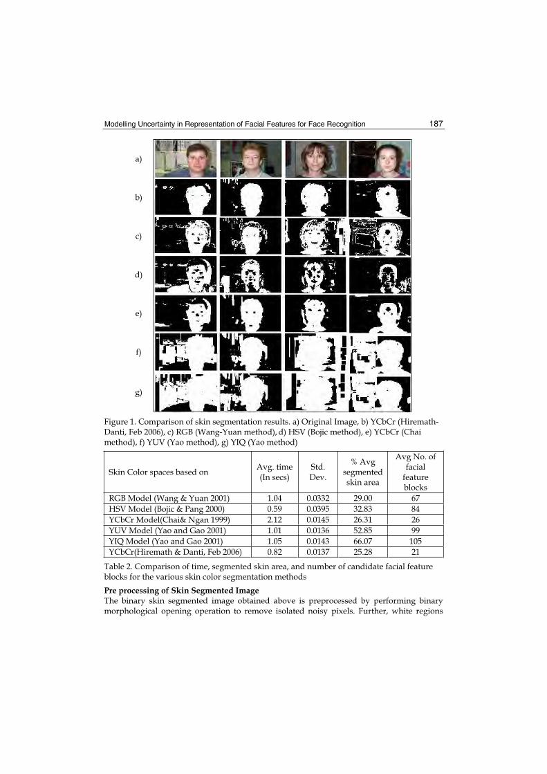
Modelling Uncertainty in Representation of Facial Features for Face Recognition 187
a)
b)
c)
d)
e)
f)
g)
Figure 1. Comparison of skin segmentation results. a) Original Image, b) YCbCr (Hiremath-Danti, Feb 2006), c) RGB (Wang-Yuan method), d) HSV (Bojic method), e) YCbCr (Chai method), f) YUV (Yao method), g) YIQ (Yao method)
Skin Color spaces based on Avg. time(In secs)
Std. Dev.
% Avg segmentedskin area
Avg No. of facial
featureblocks
RGB Model (Wang & Yuan 2001) 1.04 0.0332 29.00 67 HSV Model (Bojic & Pang 2000) 0.59 0.0395 32.83 84 YCbCr Model(Chai& Ngan 1999) 2.12 0.0145 26.31 26 YUV Model (Yao and Gao 2001) 1.01 0.0136 52.85 99 YIQ Model (Yao and Gao 2001) 1.05 0.0143 66.07 105 YCbCr(Hiremath & Danti, Feb 2006) 0.82 0.0137 25.28 21
Table 2. Comparison of time, segmented skin area, and number of candidate facial feature blocks for the various skin color segmentation methods Pre processing of Skin Segmented Image The binary skin segmented image obtained above is preprocessed by performing binary morphological opening operation to remove isolated noisy pixels. Further, white regions

Face Recognition 188
may contain black holes these black holes may be of any size and are filled completely. The binary skin image is labeled using the region labeling algorithm and their feature moments, such as center of mass ( yx, ), orientation θ , major axis length, minor axis length and area, are computed (Jain, A.K., 2001; Gonzalez, R.C., et al., 2002). By the observation of several face regions under analysis, it is found that the face regions are oriented in the range of °±45
degrees in the case of frontal view of the face images. Only such regions are retained in the binary skin image for further consideration. The remaining regions are considered as non face regions and are removed from the binary skin image. The observation of several real faces also revealed that the ratio of height to width of each face region is approximately 2, only such regions are retained. Further, though the skin regions of different sizes are successfully segmented, it is found that the potential facial features are miss-detected whenever the face area is less than 500 pixels. Hence, the regions, whose area is more than the 500 pixels are considered for the face detection process. The resulting binary skin image after the preprocessing and applying the above constraints is expected to contain potential face regions (Fig 2(a), (b)).
a) b) c)
Figure 2. Results of Skin color segmentation a) Original Image b) Potential face regions in gray scale image c) Sobel Filtered Binary image
2.2 Face Detection
Each potential face region in the binary image is converted into gray scale image as shown in Figure 2.(b) and then each face region is passed on to our fuzzy face model to decide whether the face is present in that region or not, by the process of facial feature extraction using the fuzzy rules (Hiremath & Danti Dec. 2005). The detailed face detection process, which detects multiple faces in an input image, is described in Figure 3.
Figure 3. Overview of the multiple face detection process
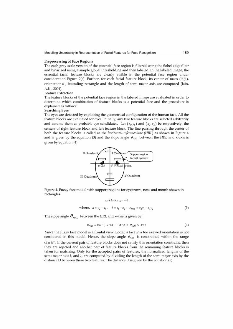
Modelling Uncertainty in Representation of Facial Features for Face Recognition 189
Preprocessing of Face Regions The each gray scale version of the potential face region is filtered using the Sobel edge filter and binarized using a simple global thresholding and then labeled. In the labeled image, the essential facial feature blocks are clearly visible in the potential face region under consideration Figure 2(c). Further, for each facial feature block, its center of mass ( yx, ),orientationθ , bounding rectangle and the length of semi major axis are computed (Jain, A.K., 2001). Feature Extraction The feature blocks of the potential face region in the labeled image are evaluated in order to determine which combination of feature blocks is a potential face and the procedure is explained as follows: Searching Eyes The eyes are detected by exploiting the geometrical configuration of the human face. All the feature blocks are evaluated for eyes. Initially, any two feature blocks are selected arbitrarily and assume them as probable eye candidates. Let ( 11, yx ) and ( 22, yx ) be respectively, the centers of right feature block and left feature block. The line passing through the center of both the feature blocks is called as the horizontal-reference-line (HRL) as shown in Figure 4 and is given by the equation (3) and the slope angle HRLθ between the HRL and x-axis is given by equation (4).
Figure 4. Fuzzy face model with support regions for eyebrows, nose and mouth shown in rectangles
0=++ HRLcbyax
where, 21122112 ,, yxyxcxxbyya HRL −=−=−= (3)
The slope angle HRLθ between the HRL and x-axis is given by:
2/2/,)/(tan 1 πθπθ ≤≤−−= −HRLHRL ba (4)
Since the fuzzy face model is a frontal view model, a face in a too skewed orientation is not considered in this model. Hence, the slope angle HRLθ is constrained within the range of 45± . If the current pair of feature blocks does not satisfy this orientation constraint, then they are rejected and another pair of feature blocks from the remaining feature blocks is taken for matching. Only for the accepted pairs of features, the normalized lengths of the semi major axis l1 and l2 are computed by dividing the length of the semi major axis by the distance D between these two features. The distance D is given by the equation (5).

Face Recognition 190
( ) ( )[ ] 2/1221
221 yyxxD −+−= (5)
Let 21 θθ and are the orientations of the above accepted feature blocks. The evaluation function EEye is computed using the equation (6) to check whether the current pair of features is a potential eye pair or not.
( ) ( ) ( ) ( )( )[ ]22
21
221
221 12.1exp HRLHRLEye llllE θθθθ −+−+−++−−= (6)
This evaluation function value ranges from 0 to 1 and it can be given the interpretation of a probability value. The constant 1.2 is the mean of the negative exponential distribution, which is determined empirically with respect to the sample images considered for experimentation to optimize higher detection rate with lower false detections. Hence, higher the evaluation value EEye higher is the probability of the two selected feature blocks to be eyes. If this evaluation value is greater than an empirical threshold value 0.7, then these two feature blocks are accepted as the potential eye pair candidate. Otherwise, this pair of blocks is rejected and another pair of feature blocks is selected. For potential eye pair candidate, the fuzzy face model is constructed and the other facial features are searched as follows.Construction of Fuzzy Face Model It is assumed that every human face is having the same geometrical configuration and the relative distances between the facial features are less sensitive to poses and expressions (Yang et al. 2002). The fuzzy face model is constructed with respect to the above potential eye candidates. A line perpendicular to the HRL at the mid point of the two eyes is called as vertical reference line (VRL). Let (p,q) be the mid point of the line segment joining the centers of the two eye candidates. Then the equation of the VRL is given by equation (7).
0=+− VRLcaybx (7)
These two reference lines (HRL and VRL) are used to partition the facial area into quadrants as shown in Figure 4. The vertical and horizontal distances of the facial features namely, eyebrows, nose and mouth are empirically estimated in terms of the distance D between the centers of the two eyes on the basis of the observations from several face images. The notations MouthNoseEyebrows VandVV , denote the vertical distances of the centers of eyebrows, nose and mouth from the HRL which are estimated as 0.3D, 0.6D and 1.0D respectively. The notations MouthNoseEyebrows HandHH , denote the horizontal distances of the centers of eyebrows, nose and mouth from the VRL which are estimated as 0.5D, 0.05D and 0.1Drespectively. The facial features are enclosed by the rectangles to represent the support regions, which confine the search area for facial features. This completes the construction of the fuzzy face model with respect to the selected potential eye pair candidate in the given face region as shown in Figure 4. Further, the fuzzy face model is used to determine which combination of the feature blocks is a face. Searching Eyebrows, Nose and Mouth The searching process proceeds to locate the other potential facial features, namely eyebrows, nose and mouth with respect to the above potential eye pair candidate. The support regions for eyebrows, nose and mouth are empirically determined using fuzzy rules as given in Table 3. Then these support regions are searched for facial features. For illustration, we take the left eyebrow feature as an example to search. Let a feature block K

Modelling Uncertainty in Representation of Facial Features for Face Recognition 191
be a potential left eyebrow feature. The horizontal distance hLeb and the vertical distance vLeb
of the centroid of the Kth feature from the VRL and HRL, respectively, are computed using the equation (8).
Vertical distances Horizontal distances Feature(j)
jvminjvmax jv jvσ
jhminjhmax jh jhσ
Eyebrows 0.02 0.38 0.2 0.06 0.24 0.65 0.45 0.07 Nose 0.30 0.90 0.6 0.10 -0.2 0.2 0.0 0.07
Mouth 0.45 1.35 0.9 0.15 -0.3 0.3 0.0 0.10
Table 3. Emperically determined distances of the facial features (normalized by D)
( ) 2/122 ba
cyaxbh VRLKKLeb
+
+−= and ( ) 2/122 ba
cybxav HRLKKLeb
+
++= , (8)
Treating Lebh and Lebv as the fuzzy quantities to represent the possible location of the potential left eyebrow feature, the fuzzy membership values
Lebhμ andLebvμ , respectively, are
defined using the trapezoidal fuzzy membership function (Hines & Douglas 1990). In particular, the membership function
Lebvμ is defined using the equation (9) and Table 3.
≥
≤≤−
−≤≤
≤≤−−
≤
=
)max(,0
)max(,)(max
)(max
)(,1
)(min,)min(
)min(
min,0
)(
LebLeb
LebLebLeb
LebLeb
Leb
LebLebLeb
LebLeb
LebLeb
Lebv
vvif
vvifv
vvvif
vvifvvv
vvif
vLeb
ββ
βα
αα
μ (9)
Similarly, the membership function Lebhμ is defined. The support region for the potential left
eyebrow feature is the set of values hLeb and vLeb whose fuzzy membership values are non-zero. The Figure 5(a) shows the graph of the trapezoidal fuzzy membership function
jvμ for
the vertical distance of the jth feature and the support region for the left eyebrow is shown in Figure 5(b). To evaluate Kth feature block in the support region for left eyebrow, the value of the evaluation function EK is given by the equation (10). The EK value ranges from 0 to 1 and represents the probability that the feature block K is a left eyebrow.
Figure 5. Trapezoidal fuzzy membership functionjvμ for the vertical distance of the jth facial
feature b) Support region for left eyebrow in the I quadrant of face model
Face Recognition 192
−−+
−−=
22
2/2.1exp
2/2.1exp
2
1
DHh
DVv
E EyebrowsLebEyebrowsLebK (10)
Similarly, evaluation value is computed for all the feature blocks present in that support region of the left eyebrow. The evaluation value ELeb is a fuzzy quantity represented by the set of EK values with their corresponding fuzzy membership values Kμ . The membership value Lebμ corresponding to ELeb is obtained by the min-max fuzzy composition rule (Klir & Yuan 2000) given by the equations (11) and (12). The feature block having the evaluation value ELeb with the corresponding Lebμ found in the support region of the left eyebrow is the potential left eyebrow feature with respect to the current pair of potential eye candidates.
( )KK vhK μμμ ,min= , for each K (11)
{ }KK
Leb μμ max= (12)
Similarly, the right eyebrow, nose and mouth are searched in their respective support regions determined by appropriately defining the membership functions for the fuzzy distances (horizontal and vertical) from the centroid of these facial features, and their fuzzy evaluation values are computed by applying the min-max fuzzy composition rule. The overall fuzzy evaluation E for the fuzzy face model is defined as the weighted sum of the fuzzy evaluation values of the potential facial features namely, for the eye, left eyebrow, right eyebrow, nose and mouth, respectively. The weights are adjusted to sum to unity as given in the equation (13). The membership value Eμ corresponding to E is obtained by the fuzzy composition rule as given by the equation (14).
bLebNoseMouthEye EEEEEE Re05.005.02.03.04.0 ++++= (13)
{ }bLebNoseMouthE Re,,,min μμμμμ = (14)
Above procedure is repeated for every potential eye pair candidate and get the set of fuzzy faces. These fuzzy faces are represented by the set of E values with their corresponding membership values Eμ . Finally, the most probable face is obtained by the defuzzification process as given by the equation (15).
{ }EE
E μμΩ∈
= maxmax (15)
Then the E value corresponding to maxEμ is the defuzzified evaluation value ED of the face. If there are more than one E value corresponding to maxEμ , the maximum among those values is the defuzzified evaluation value ED of the face. Finally, the potential eyes, eyebrows, nose and mouth features corresponding to the overall evaluation value ED
constitute the most probable face in the given face region, provided ED is greater than the empirical threshold value 0.7. Otherwise this face region is rejected. The face detection results are shown in Figure 6, where (a) display the feature extraction in which facial features are shown in bounding boxes (Jain 2001) and (b) shows detected face in rectangular box. (Hiremath P.S. & Danti A. Feb 2006). The above procedure is repeated for every potential face region to detect possible faces in the input image.

Modelling Uncertainty in Representation of Facial Features for Face Recognition 193
Figure 6. Results of Face Detection a) Facial Feature extraction b) Detected face in box
2.3 Experimental Results
The MATLAB 6.0 implementation of the above described procedure on Pentium IV @ 2.6 GHz yields the success rate of 96.16%. The average time taken to detect one face is about 0.78 sec, which depends on the size of the potential face region. The search area for the facial feature extraction is confined to only the total area covered by the support regions i.e. 0.67D2, (D is distance between eyes) which is considerably very small compared to that of the image size. This reduced search area leads to the reduction in the detection time to a great extent. Sample detection results are shown in Figure 7 and Figure 8 with detected faces enclosed in rectangular boxes. Due to the constraints of the face model, miss-detection occurs due to several reasons i.e. profile (side) view faces, abnormal lighting conditions, face occluded by hair, very small face sizes, face occluded by hand and too dark shadow on faces as shown in Figure 9. The comparison of different state of the art detectors proposed by (Shih and Liu 2004, we refer as S-L method) and (Schneiderman and Kanade 2000, we refer as S-K method) and (Hiremath and Danti, Dec. 2005, we refer as H-D method) is given in Table 4. It is observed that, fuzzy face model approach based on skin color segmentation (H-D method) is comparable to others in terms of detection rate and very low in both detection time and false detections.
Method Det.Rate (%)
False detection
Det. Time (secs) Dataset No. of
imagesNo. of faces
S-L method 98.2 2 notreported MIT-CMU 92 282
S-K method 94.4 65 5 MIT-CMU 125 483
H-D method 96.1 02 0.78 CIT, FERET, Internet 650 725
Table 4. Comparison of performance
Figure 7. Sample detection results for single as well as multiple human faces with sizes, poses, expressions and complex backgrounds
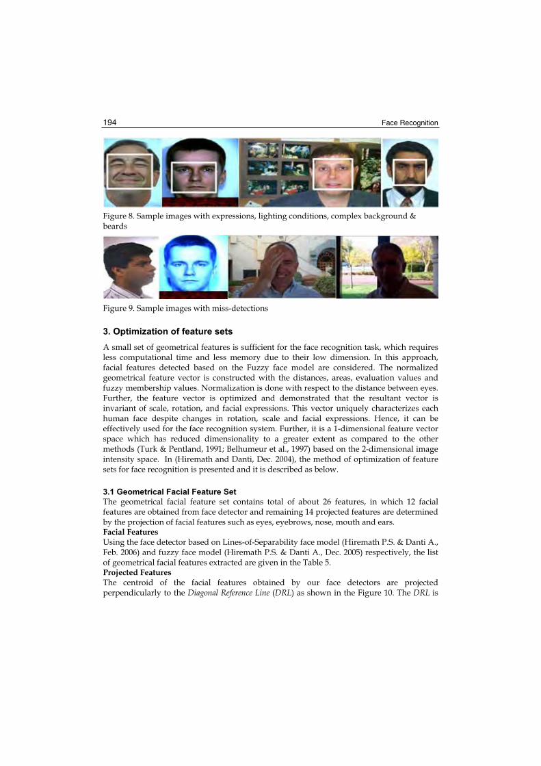
Face Recognition 194
Figure 8. Sample images with expressions, lighting conditions, complex background & beards
Figure 9. Sample images with miss-detections
3. Optimization of feature sets
A small set of geometrical features is sufficient for the face recognition task, which requires less computational time and less memory due to their low dimension. In this approach, facial features detected based on the Fuzzy face model are considered. The normalized geometrical feature vector is constructed with the distances, areas, evaluation values and fuzzy membership values. Normalization is done with respect to the distance between eyes. Further, the feature vector is optimized and demonstrated that the resultant vector is invariant of scale, rotation, and facial expressions. This vector uniquely characterizes each human face despite changes in rotation, scale and facial expressions. Hence, it can be effectively used for the face recognition system. Further, it is a 1-dimensional feature vector space which has reduced dimensionality to a greater extent as compared to the other methods (Turk & Pentland, 1991; Belhumeur et al., 1997) based on the 2-dimensional image intensity space. In (Hiremath and Danti, Dec. 2004), the method of optimization of feature sets for face recognition is presented and it is described as below.
3.1 Geometrical Facial Feature Set
The geometrical facial feature set contains total of about 26 features, in which 12 facial features are obtained from face detector and remaining 14 projected features are determined by the projection of facial features such as eyes, eyebrows, nose, mouth and ears. Facial FeaturesUsing the face detector based on Lines-of-Separability face model (Hiremath P.S. & Danti A., Feb. 2006) and fuzzy face model (Hiremath P.S. & Danti A., Dec. 2005) respectively, the list of geometrical facial features extracted are given in the Table 5. Projected Features The centroid of the facial features obtained by our face detectors are projected perpendicularly to the Diagonal Reference Line (DRL) as shown in the Figure 10. The DRL is

Modelling Uncertainty in Representation of Facial Features for Face Recognition 195
the line bisecting the first quadrant in the HRL-VRL plane and is a locus of point (x,y)equidistant from HRL and VRL. The equation of the DRL is given by:
0=++ CByAx , where the coefficients A, B, and C are given by: (16)
)(),(),( VRLHRL ccCbaBbaA −=+=−= (17)
Feature Description Feature Description EEyes Evaluation value of eyes ERear Evaluation value of right ear
ELebEvaluation value of left eyebrow E Overall evaluation value of the
face
ERebEvaluation value of right eyebrow Lebμ
Membership value of left eyebrow
ENose Evaluation value of nose bReμMembership value of right eyebrow
EMouth Evaluation value of mouth Noseμ Membership value of nose
ELear Evaluation value of left ear Mouthμ Membership value of mouth
Table 5. List of geometrical features extracted from face detectors
Figure 10. Projection of features on to DRLDistance Ratio Features The distance ratios are computed as described in the following. Let ),( KK yx be the centroid K of the kth feature (e.g. left eyebrow in the Figure 10). Let KP be the projection of point K on the DRL. Then, the following distances are computed:
22 BA
CByAxKP KKK
+
++= (Perpendicular distance) (18)
22 )()( KK yqxpMK −+−= (Radial distance) (19)
22KK KPMKMP −= (Diagonal distance) (20)

Face Recognition 196
KK
Leb MPKPR = (Distance ratio) (21)
The notation, LebR denote the distance ratio obtained by the projection of left eyebrow. Similarly the distance ratios arLearMouthNosebLe RandRRRRRR ReReRe ,,,,, are determined, respectively for left eye, right eye, right eyebrow, nose, mouth, left ear and right ear. Distance Ratio Features in Combination The distances of all the facial features along the DRL are used to compute the distance ratios for the combination of facial features as follows.
ye
LeyeyeLeye MP
MPR
ReRe2 = (Left Eye to Right Eye) (22)
b
LebbLeb MP
MPR
ReRe2 = (Left Eyebrow to Right Eyebrow) (23)
m
nMN MP
MPR =2 (Nose to Mouth) (24)
ar
LeararLear MP
MPR
ReRe2 = (Left Ear to Right Ear) (25)
Area Features The centroids of the eyes, eyebrows, nose and mouth are connected in triangles as shown in the Figure 11. The areas covered by the triangles are used to determine the area features. In Figure 11(a), e1 and e2 denote right and left eyes respectively; n and m denote nose and mouth respectively. The coordinates ),(,),(,),(,),( 44332211 yxandyxyxyx are the centroids of right eye, left eye, nose, and mouth respectively.
Figure 11. Triangular area features (a) Areas formed by eyes, nose, and mouth (b) Areas formed by eyebrows, nose, and mouth
The triangular area Aen formed by eyes and nose; and, the triangular area Aem formed by eyes and mouth are computed as given below.
)()(
)()(5.0
3232
3131
yyxxyyxx
Aen −−−−
= & )()(
)()(5.0
4242
4141
yyxxyyxx
Aem −−−−
= (26)
em
enEyes A
AA = (27)

Modelling Uncertainty in Representation of Facial Features for Face Recognition 197
Then the ratio of areas covered by eyes, nose and mouth is given by the equation (27). Similarly, in Figure 11(b), b1 and b2 denote right and left eyebrows respectively, and n and mdenote nose and mouth respectively. The coordinates ),(,),( 2211 yxyx , ),(),,( 4433 yxandyx are the centroids of right eyebrow, left eyebrow, nose, and mouth respectively. The triangular area Aebn formed by eyebrows and nose; and, the triangular area Aebm formed by eyebrows and mouth are computed as given below.
)()(
)()(5.0
3232
3131
yyxxyyxx
Aebn −−−−
= & )()(
)()(5.0
4242
4141
yyxxyyxx
Aebm −−−−
= (28)
ebm
ebnEyebrows A
AA = (29)
Then the ratio of areas covered by eyebrows, nose and mouth is given by the equation (29). The projected features are listed in the Table 6.
Feature Description Feature Description RLeye Distance ratio by left eye RRear Distance ratio by right ear RReye Distance ratio by right eye RLeye2Reye Distance ratio by left and right eyes RLeb Distance ratio by left
eyebrowRReb2Leb Distance ratio by left & right
eyebowsRReb Distance ratio by right
eyebrowRN2M Distance ratio by nose and mouth
RNose Distance ratio by nose RLear2Rear Distance ratio by left ear and right ear
RMouth Distance ratio by mouth AEyes Area ratio by eyes, nose and mouth RLear Distance ratio by left ear AEyebrows Area ratio by eyebrows, nose and
mouth
Table 6. List of projected features
Final geometrical features include 26 features, in which 12 features are from the Table 5 and 14 features are from the Table 6.
3.2 Optimization of Features Sets
Three subsets of features from 26 features in different combinations are considered for optimization. The subset A, B, C consist of 14, 6, 14 features, respectively as given below.
),,,,,
,,,,,,,(
Re222ReRe2
ReRe,Re
EyebrowsEyesarLearMNLebbyeLeye
arLearMouthNosebLebyeLeye
AARRRR
RRRRRRRRSubsetA = (30)
),,,,,( 22Re EyebrowsEyesMNLebbEyes AARREEBSubset = (31)
),,,,,
,,,,,,,,(
22Re
ReRe
EyebrowsEyesNoseMouthLebbMouth
NosebLebEyesMouthNosebLeb
AARREE
EEEECSubset μμμμ= (32)
The every feature subset is optimized by the maximal distances between the classes and minimal distances between the patterns of one class. Here each class represents one person

Face Recognition 198
and the different images of one person were considered as patterns. The effectiveness of every feature subset is determined by the evaluation function F as given below.
=
=
−
−
== k
iim
k
iid
m
d
MM
DM
DDF
1
2
1
2
)(
)(
wheren
f
M
n
jij
i== 1 ,
k
M
M
k
ii
m== 1 ,
1
)(
1
2
−
−
= =k
MM
D
k
iim
m
1
)(
1
2
−
−
= =n
fM
D
n
jiji
i ,k
D
M
k
ii
d== 1 ,
1
)(
1
2
−
−
= =
k
DM
D
k
iid
d (33)
where Mi and Di are mean and variance of the feature values fij for (j =1 to k) k images of the i-th person respectively, Mm and Md are mean of Mi and Di respectively. The F value is the ratio of the measures of dispersion of sample standard deviations and of the sample means of the feature values in the k sample images of a class. For illustration we have used ORL face database, which contain 40 subjects or classes and each of 10 variations. The Figure 12 shows the optimization of feature subsets in which F values along the y-axis are plotted for 40 classes along the x-axis. The lower F value indicates the stronger invariance property of the feature subset with respect to scale, rotation and facial expressions. In the Figure 12 it shows that the feature subset C is well optimized with the lowest F values compared to other subsets and, hence it corresponds to a better feature subset.
Figure 12. Optimization of subsets of features
Invariance Property The above feature Subset C is considered as the most optimized geometrical feature vector for face recognition and is invariant to scaling, rotation, and facial expressions, because the relative geometrical distances between the facial features such as eyes, nose, mouth, and eyebrows vary proportionally with respect to scaling, rotation, and facial expressions, and their feature values remain nearly constant. Hence the optimized feature vector characterizes each human face uniquely. The Figure 13 illustrates the invariance property of
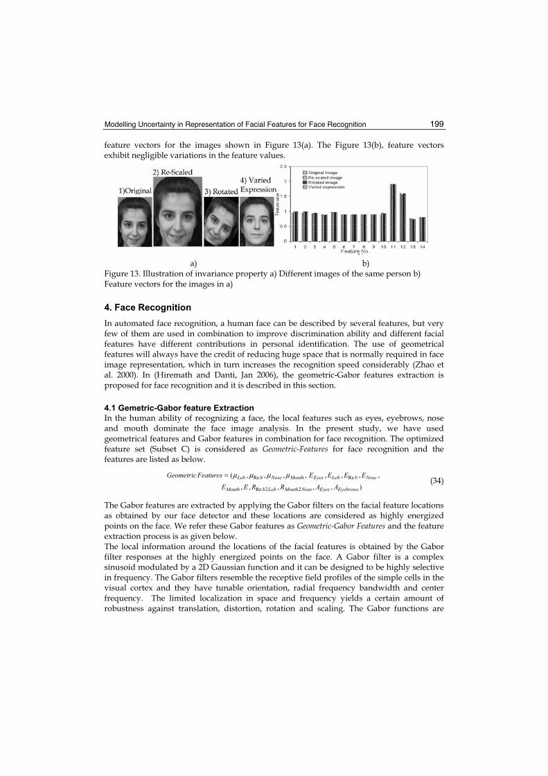
Modelling Uncertainty in Representation of Facial Features for Face Recognition 199
feature vectors for the images shown in Figure 13(a). The Figure 13(b), feature vectors exhibit negligible variations in the feature values.
a) b) Figure 13. Illustration of invariance property a) Different images of the same person b) Feature vectors for the images in a)
4. Face Recognition
In automated face recognition, a human face can be described by several features, but very few of them are used in combination to improve discrimination ability and different facial features have different contributions in personal identification. The use of geometrical features will always have the credit of reducing huge space that is normally required in face image representation, which in turn increases the recognition speed considerably (Zhao et al. 2000). In (Hiremath and Danti, Jan 2006), the geometric-Gabor features extraction is proposed for face recognition and it is described in this section.
4.1 Gemetric-Gabor feature Extraction
In the human ability of recognizing a face, the local features such as eyes, eyebrows, nose and mouth dominate the face image analysis. In the present study, we have used geometrical features and Gabor features in combination for face recognition. The optimized feature set (Subset C) is considered as Geometric-Features for face recognition and the features are listed as below.
),,,,,
,,,,,,,,(
22Re
ReRe
EyebrowsEyesNoseMouthLebbMouth
NosebLebEyesMouthNosebLeb
AARREE
EEEEFeaturesGeometric μμμμ= (34)
The Gabor features are extracted by applying the Gabor filters on the facial feature locations as obtained by our face detector and these locations are considered as highly energized points on the face. We refer these Gabor features as Geometric-Gabor Features and the feature extraction process is as given below. The local information around the locations of the facial features is obtained by the Gabor filter responses at the highly energized points on the face. A Gabor filter is a complex sinusoid modulated by a 2D Gaussian function and it can be designed to be highly selective in frequency. The Gabor filters resemble the receptive field profiles of the simple cells in the visual cortex and they have tunable orientation, radial frequency bandwidth and center frequency. The limited localization in space and frequency yields a certain amount of robustness against translation, distortion, rotation and scaling. The Gabor functions are

Face Recognition 200
generalized by Daugman (Daugman 1980) to the following 2D form in order to model the receptive fields of the orientation selective simple cells. The Gabor responses describe a small patch of gray values in an image I(x) around a given pixel x=(x,y)T. It is based on a wavelet transformation, given by the equation:
xdxxxIxR ii ′′−′= )()()( ψ (35)
This is a convolution of image with a family of Gabor kernels
−=−−
222
2 2
2
22
)(
σσ
σψ eee
kx xjk
xki
ii
i
, , where ==μ
μ
θθ
sin
cos
v
v
iy
ixi k
kkk
k (36)
Each iψ is a plane wave characterized by the vector ik enveloped by a Gaussian function,
where σ is the standard deviation of this Gaussian. The center frequency of thi filter is given by the characteristic wave vector ik , in which scale and orientation given by ),( μθvk .The first term in the Gabor kernel determines the oscillatory part of the kernel and the second term compensates for the DC value of the kernel. Subtracting the DC response, Gabor filter becomes insensitive to the overall level of illumination. The decomposition of an image into these states is called wavelet transform of the image given by equation (35). Convolving the input image with complex Gabor filters with 5 spatial frequencies )4,...0( =vand 8 orientations )7,...0( =μ will capture the whole frequency spectrum, both amplitude and phase, as shown in the Figure 14.
Figure 14. Gabor filters w.r.t. 5 Frequencies and 8 Orientations
In the Figure 15, an input face image (a), the highly energized points (b) and the amplitude of the responses (c) to the above Gabor filters are shown. Several techniques found in the literature for Gabor filter based face recognition consist of obtaining the response at grid points representing the entire facial topology using elastic graph matching for face coding (Kotropoulos et al. April 2000; Wiskott et al.1999; Duc et al. 1999), which generate the high dimensional Gabor feature vector. However, instead of using the graph nodes on entire face, we have utilized only the locations of the facial features such as eyes, eyebrows, nose, and mouth extracted by our face detector (Hiremath P.S. & Danti March 2005) as the highly energized face points (Figure 15(b)) and Gabor filter responses are obtained at these points only. This approach leads to reduced computational complexity and improved performance on account of the low dimensionality of the extended feature vector, which is demonstrated
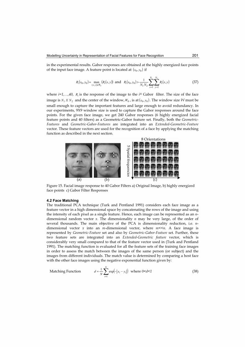
Modelling Uncertainty in Representation of Facial Features for Face Recognition 201
in the experimental results. Gabor responses are obtained at the highly energized face points of the input face image. A feature point is located at ( )00 , yx if
( ) ( )( )yxRyxR iWyx
i ,max,0),(
00∈
= and ( ) ( )= =
>1 2
1 121
00 ,1
,
N
x
N
yii yxR
NNyxR (37)
where i=1,…,40, iR is the response of the image to the ith Gabor filter. The size of the face image is 21 NXN and the center of the window, 0W , is at ( )00 , yx . The window size W must be small enough to capture the important features and large enough to avoid redundancy. In our experiments, 9X9 window size is used to capture the Gabor responses around the face points. For the given face image, we get 240 Gabor responses (6 highly energized facial feature points and 40 filters) as a Geometric-Gabor feature set. Finally, both the Geometric-Features and Geometric-Gabor-Features are integrated into an Extended-Geometric-Featurevector. These feature vectors are used for the recognition of a face by applying the matching function as described in the next section.
Figure 15. Facial image response to 40 Gabor Filters a) Original Image, b) highly energized face points c) Gabor Filter Responses
4.2 Face Matching
The traditional PCA technique (Turk and Pentland 1991) considers each face image as a feature vector in a high dimensional space by concatenating the rows of the image and using the intensity of each pixel as a single feature. Hence, each image can be represented as an n-dimensional random vector x. The dimensionality n may be very large, of the order of several thousands. The main objective of the PCA is dimensionality reduction, i.e. n-dimensional vector x into an m-dimensional vector, where m<<n. A face image is represented by Geometric-Feature set and also by Geometric-Gabor-Feature set. Further, these two feature sets are integrated into an Extended-Geometric feature vector, which is considerably very small compared to that of the feature vector used in (Turk and Pentland 1991). The matching function is evaluated for all the feature sets of the training face images in order to assess the match between the images of the same person (or subject) and the images from different individuals. The match value is determined by comparing a host face with the other face images using the negative exponential function given by:
Matching Function ( )=
−−=N
iii yx
Nd
1
exp1 where 0<d<1 (38)

Face Recognition 202
where xi and yi are the feature elements of the face images X and Y, respectively, N is the total number of elements of the feature. The results of the matching performance for the database faces using the Geometric-Feature set, the Geometric-Gabor-Feature set and the Extended-Geometric-Feature set are shown in the Figure 17(a), (b) and (c), respectively. The match value dEGF for an Extended-Geometric-Feature vector is determined by the average of the match values of Geometric dGF and Geometric-Gabor dGGF feature sets as given below:
[ ]GGFGFEGF ddd +=2
1 (39)
The match values are determined using the matching function. The horizontal axis represents the face number and the vertical axis represents the match between faces for that feature set. The value of the match is within the range [0,1] and can be given probability interpretation. The match is 1, when the host face is having highest match with that of the target faces and the match is zero, when the host face is having lowest match with that of the target faces. The performance of the features are analyzed by searching for target faces that match with the given host face. The targets are different images of the same person as the host. The analysis is based on the individual assessment of the two feature sets as well as the performance when both the feature sets are integrated into the extended feature vector.
4.3 Experimental Results
For experimentation, the ORL and MIT face databases, which are the publicly available benchmark databases for evaluation, are used. The ORL database consists of 400 images, in which there are 40 subjects (persons) and each having 10 variations i.e. varying expressions, poses, lighting conditions under homogeneous background. The MIT database consists of 432 images, in which there are 16 subjects and each having 27 variations i.e. different head tilts, scales and lighting conditions under moderate background. The experimentation is done with 40 face images, which consist of 10 subjects and each of 4 variations. To illustrate the analysis of experimental results, the Figure 16 depicts face no 21 as host face and face nos. 22, 23 and 24 as its target faces, i.e. these face images pertain to the same subject (person). Results of the match between the face 21 and the other 39 faces are shown in the Figs. 17 (a), (b) and (c) for the Geometric-Feature set, the Geometric-Gabor-Feature set and the Extended-Geometric-Feature vector, respectively. In the Figure 17(a), we observe that some of the non-target faces also yield a comparable match value as that of target faces leading to recognition errors, e.g. non-target face nos. 3, 26 and 27 have match values close to that of target faces no. 23. Further, many of the non-target faces have match values greater than 0.5 leading to the poor discrimination ability of the geometric feature set. Similar observations can be made in the Figure 17(b), but the discrimination ability of Geometric-Gabor feature set is found to be better than the geometric feature set. Only few non-target faces have match values greater than 0.4 and close to the target faces. However, still improved match results are found in case of the integrated feature vector combining geometric as well as Geometric-Gabor features and are depicted in Figure 17(c). All the non-target faces have their match values much less than 0.4 and are well discriminated from the target faces leading to enhanced recognition rate. The possibility of a good match of the non-target faces on individual feature sets have been reduced and such faces are well discriminated by the integration of both the feature sets as shown in the Figure 17(c). Similar discrimination results are reported when comparing the
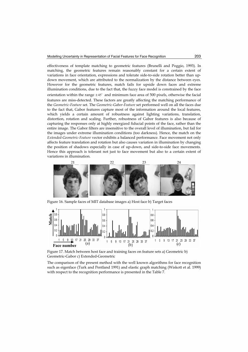
Modelling Uncertainty in Representation of Facial Features for Face Recognition 203
effectiveness of template matching to geometric features (Brunelli and Poggio, 1993). In matching, the geometric features remain reasonably constant for a certain extent of variations in face orientation, expressions and tolerate side-to-side rotation better than up-down movement, which are attributed to the normalization by the distance between eyes. However for the geometric features, match fails for upside down faces and extreme illumination conditions, due to the fact that, the fuzzy face model is constrained by the face orientation within the range 45± and minimum face area of 500 pixels, otherwise the facial features are miss-detected. These factors are greatly affecting the matching performance of the Geometric-Feature set. The Geometric-Gabor-Feature set performed well on all the faces due to the fact that, Gabor features capture most of the information around the local features, which yields a certain amount of robustness against lighting variations, translation, distortion, rotation and scaling. Further, robustness of Gabor features is also because of capturing the responses only at highly energized fiducial points of the face, rather than the entire image. The Gabor filters are insensitive to the overall level of illumination, but fail for the images under extreme illumination conditions (too darkness). Hence, the match on the Extended-Geometric-Feature vector exhibits a balanced performance. Face movement not only affects feature translation and rotation but also causes variation in illumination by changing the position of shadows especially in case of up-down, and side-to-side face movements. Hence this approach is tolerant not just to face movement but also to a certain extent of variations in illumination.
Figure 16. Sample faces of MIT database images a) Host face b) Target faces
Figure 17. Match between host face and training faces on feature sets a) Geometric b) Geometric-Gabor c) Extended-Geometric
The comparison of the present method with the well known algorithms for face recognition such as eigenface (Turk and Pentland 1991) and elastic graph matching (Wiskott et al. 1999) with respect to the recognition performance is presented in the Table 7.
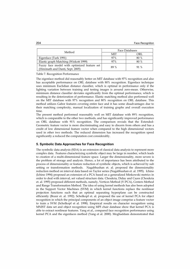
Face Recognition 204
Face Databases Method MIT ORL Eigenface (Turk 1991) 97% 80 % Elastic graph Matching (Wiskott 1999) 97% 80 % Fuzzy face model with optimized feature set (Hiremath and Danti, Sept. 2005) 89 % 91 %
Table 7. Recognition Performance
The eigenface method did reasonably better on MIT database with 97% recognition and also has acceptable performance on ORL database with 80% recognition. Eigenface technique uses minimum Euclidian distance classifier, which is optimal in performance only if the lighting variation between training and testing images is around zero-mean. Otherwise, minimum distance classifier deviates significantly from the optimal performance, which is resulting in the deterioration of performance. Elastic matching method also performed well on the MIT database with 97% recognition and 80% recognition on ORL database. This method utilizes Gabor features covering entire face and it has some disadvantages due to their matching complexity, manual localization of training graphs and overall execution time.The present method performed reasonably well on MIT database with 89% recognition, which is comparable to the other two methods, and has significantly improved performance on ORL database with 91% recognition. The comparison reveals that the Extended-Geometric feature vector is more discriminating and easy to discern from others and has a credit of low dimensional feature vector when compared to the high dimensional vectors used in other two methods. The reduced dimension has increased the recognition speed significantly a reduced the computation cost considerably.
5. Symbolic Data Approaches for Face Recognition
The symbolic data analysis (SDA) is an extension of classical data analysis to represent more complex data. Features characterizing symbolic object may be large in number, which leads to creation of a multi-dimensional feature space. Larger the dimensionality, more severe is the problem of storage and analysis. Hence, a lot of importance has been attributed to the process of dimensionality or feature reduction of symbolic objects, which is achieved by sub setting or transformation methods. Nagabhushan et. al. proposed the dimensionality reduction method on interval data based on Taylor series (Nagabhushan et. al. 1995). Ichino (Ichino 1994) proposed an extension of a PCA based on a generalized Minkowski metrics in order to deal with interval, set valued structure data. Choukria, Diday and Cazes (Choukria et. al. 1995) proposed different methods, namely, Vertices Method (V-PCA), Centers Method and Range Transformation Method. The idea of using kernel methods has also been adopted in the Support Vector Machines (SVM) in which kernel functions replace the nonlinear projection functions such that an optimal separating hyperplane can be constructed efficiently (Bozer et. al. 1992). Scholkopf et. al. proposed the use of kernel PCA for object recognition in which the principal components of an object image comprise a feature vector to train a SVM (Scholkopf et al. 1998). Empirical results on character recognition using MNIST data set and object recognition using MPI chair database show that kernel PCA is able to extract nonlinear features. Yang et al., compared face recognition performance using kernel PCA and the eigenfaces method (Yang et al. 2000). Moghaddam demonstrated that

Modelling Uncertainty in Representation of Facial Features for Face Recognition 205
kernel PCA performed better than PCA for face Recognition (Moghaddam 2002). Chengjun Liu extended kernel PCA method to include fractional power polynomial models for enhanced face recognition performance. (Chengjun Liu 2004). In (Hiremath and Prabhakar, 2006), an integrated approach based on symbolic data analysis and kernel PCA for face recognition is explored.
5.1 Symbolic Kernel PCA for Face Recognition
This section details the face recognition method using symbolic kernel PCA method (Hiremath and Prabhakar, 2006). In the training phase, firstly, the symbolic faces are constructed for a given face database images. Secondly, symbolic kernel PCA is applied to the symbolic faces in order to nonlinearly derive low dimensional interval type features that incorporate higher order statistics. In the classification phase, the test symbolic face is constructed for a given test face class in order to derive the symbolic kernel PCA interval-type features. Finally, a minimum distance classifier is employed for classification using appropriate symbolic dissimilarity measure. Construction of Symbolic Faces Consider the face images nΓΓΓ ,...,, 21 , each of size MN × , from a face image database. Let
{ }nΓΓ=Ω ,....,1 be the collection of n face images of the database, which are first order objects. Each object Ω∈Γl , ,,...,1 nl = is described by a feature vector ( )pYY
~,...,
~1 , of length
,NMp= where each component ,,...,1,~
pjYj = is a single valued variable representing the intensity values of the face image lΓ . An image set is a collection of face images of mdifferent subjects and each subject has different images with varying expressions, orientations and illuminations. The face images are arranged from right side view to left side view. Thus there are m number of second order objects (face classes) denoted by
{ }mcccF .,..,, 21= , each consisting of different individual images, Ω∈Γl , of a subject. The view range of each face class is partitioned into q sub face classes and each sub face class contains r number of images. The feature vector of thk sub face class k
ic of thi face class ic , where ,,,2,1 qk = is described by a vector of p interval variables pYY ,...,1 , and is of length NMp= .
The interval variable jY of thk sub face class kic of thi face class is described as:
],[)(kij
kij
kij xxcY = (40)
where kijx and k
ijx are minimum and maximum intensity values, respectively, among jth
pixels of all the images of sub face class kic . This interval incorporates variability of thj
feature inside the thk sub face class kic .
We denote, ( ) ( )( ) .,,1,,,1,,...,1 qkmicYcYX kip
ki
ki === (41)
The vector kiX of interval variables is recorded for thk sub face class k
ic of thi face class. This vector is called as symbolic face and is represented as:
( )kipki
kiX αα ,...,1= (42)

Face Recognition 206
where pjxxcYkij
kij
kij
kij ,...,1],,[)( ===α and ;,,1 qk = .,,2,1 mi = We represent the qm symbolic
faces by a ( pqm × ) matrix X consisting of qm row vectors kiX :
[ ] pqmkiXX ×= (43)
Extraction of Non Linear Interval Type Features Let us consider the matrix X containing qm symbolic faces pertaining to the given set Ω of
images belonging to m face classes. The centers ℜ∈Ckijx of the intervals ],,[
kij
kij
kij xx=α are
given by
2
kij
kijCk
ijxx
x+
= , where ,,,1 qk = .,...,1,...,1 pjandmi == (44)
The pqm× data matrix CX containing the centers ℜ∈Ckijx of the intervals kijα for qm
symbolic faces is given by:
pqm
Cki
C XX×
= (45)
Where the p-dimensional vectors =Ck
ipCki
Cki xxX ,,1 , ( )k
ipki
ki xxX ,,
1= and =
kip
ki
ki xxX ,,1
represent the centers, lower bounds and upper bounds of the qm symbolic faces kiX ,
respectively. Let Fp →ℜΦ : be a nonlinear mapping between the input space and the feature space. For kernel PCA, the nonlinear mapping, Φ , usually defines a kernel function. Let D represent the data matrix of centers of qm symbolic faces in the feature space:
ΦΦΦΦ= )(,),(,...),(,),( 11
11
Cqm
Cm
CqCXXXXD . Let qmqmK ×ℜ∈ define a kernel matrix by
means of dot product in the feature space:
( ))()( jiij XXK Φ⋅Φ= (46)
Assume the mapped data is centered. As described in (Scholkopf et al., 1998), the eigenvalues, qmλλλ ≥≥≥ ...21 , and the eigenvectors ,,...,, 21 qmVVV of kernel matrix K can be derived by solving the following equation:
,Λ=qmAKA with [ ]qmaaA ,...,1= , { }qmdiag λλ ,...,1=Λ (47)
where qmqmA ×ℜ∈ is an orthogonal eigenvector matrix, qmqm×ℜ∈Λ a diagonal eigen value matrix with diagonal elements in decreasing order. In order to derive the eigenvector matrix
[ ]qmVVVV ,...,, 21= of symbolic kernel PCA, first, A should be normalized such that
.,...,1,12 qmuauu ==λ The eigenvector matrix, V, is then derived as follows:
ADV T= (48)

Modelling Uncertainty in Representation of Facial Features for Face Recognition 207
A subspace is extracted from the qmp × dimensional space V by selecting qmS ≤ number of eigenvectors, which contain maximum variance and are denoted by
,,...,, 21 SVVV corresponding to eigenvalues ....21 Sλλλ ≥≥≥ The thv eigenvector of V is
denoted by ( )vpvv VVV ,,1= . Since, the symbolic face kiX is located between the lower bound
symbolic face kiX and upper bound symbolic face k
iX , it is possible to find thv interval
principal component ],[kiv
kiv WW of symbolic face k
iX defined by
><
Φ−Φ+Φ−Φ=0:0:
.)()(.)()(
vjvj Vjvj
Ckij
kij
Vjvj
Ckij
kij
kiv VxxVxxW (49)
><
Φ−Φ+Φ−Φ=0:0:
.)()(.)()(
vjvj Vjvj
Ckij
kij
Vjvj
Ckij
kij
kiv VxxVxxW (50)
where ,,,1 Sv = and qmxxji
Ckij
Ckij Φ=Φ
,
)()(. Let testc be the test face class, which contains face
images of same subject with different expression, lighting condition and orientation. The test face class testc is described by a feature vector testX termed as test symbolic face of pinterval variables pYY ,...,1 , and is of length NMp= . The interval variable jY of test symbolic face is described as ],[)( )()( jtestjtesttestj xxXY = ,where ,
)( jtestx and jtestx )( are minimum and
maximum intensity values, respectively, among jth pixels of all the images of test face class testc . This interval incorporates information of the variability of thj feature inside the
test face class testc . The lower bound of test symbolic face testX is described as ( )ptesttesttesttest xxxX
)(2)(1)()(,,,= . Similarly, the upper bound is described
as ( )ptesttesttesttest xxxX )(2)(1)( ,,,= . The thv interval principal component ],[ )()( vtestvtest WW of test
symbolic face testX is computed as:
><
Φ−Φ+Φ−Φ=0:
)()(
0:
)()()(.)()(.)()(
vjvj Vjvj
Cjtestjtest
Vjvj
Cjtestjtestvtest VxxVxxW (51)
><
Φ−Φ+Φ−Φ=0:
)()(
0:
)()()( .)()(.)()(
vjvj Vjvj
Cjtestjtest
Vjvj
Cjtestjtestvtest VxxVxxW (52)
where ,,,1 Sv = and2
)()()(
)(jtestjtestC
jtestxx
x+
=Φ .
5.2 Classification Rule
When test face class testc is presented to the symbolic kernel PCA classifier, low dimensional
symbolic kernel PCA interval type features ],[ )()( vtestvtest WW are derived. Let ],[kiv
kiv WW ,
i=1,2,..., m, and ,,,1 qk = be the symbolic kernel PCA interval type features of qm symbolic

Face Recognition 208
faces. The classifier applies the minimum distance rule for classification using symbolic dissimilarity measure :δ
itestkiv
kivvtestvtesti
kivk
ivvtestvtest ccWWWWWWWW ∈→= ],[],,[min],[],,[ )()()()(δδ (53)
The symbolic kernel PCA interval type feature vector ],[ )()( vtestvtest WW is classified as
belonging to the face class, ic , using appropriate symbolic dissimilarity measure .δ Twoclasses of kernel functions widely used in kernel classifiers are polynomial kernels and Gaussian kernels defined, respectively, as:
dyxyxk )(),( ⋅= (54)
−−=
2
2
2exp),(
σ
yxyxk , where .00, >>Ν∈ kandd σ (55)
5.3 Experimental Results
The symbolic kernel PCA method is experimented with the face images of the ORL face database, which composed of 400 images with ten different images for each of the 40 distinct subjects. All the images were taken against a dark homogeneous background with the subjects in an upright, frontal position, with tolerance for some tilting and rotation of up to about o20 from frontal view to left side view and right side view. In the training phase, each face class is partitioned into three sub face classes based on view range from right side view to left side view. Each sub face class will have three images and totally nine images of one subject are used for training purpose. Thus, we obtain the 120 symbolic faces. The symbolic kernel PCA is applied to obtain the non-linear interval type features from symbolic faces. The classification phase includes construction of test symbolic face for each trial using randomly selected three images from each face class and extraction of interval type features from test symbolic face. Further, a minimum distance classifier is employed for classification using symbolic dissimilarity measure. Figure 18(a) shows some typical images of one subject of ORL database and their corresponding view based arrangement. Figure 18(b) shows the constructed symbolic faces for face class shown in (a).
(a)
(b)
Figure 18. (a) Arrangement of faces images from right to left side view belonging to one subject of ORL database. (b) Three symbolic faces of face class shown in (a) and each symbolic face summarizes the variation of feature values through the images belonging to corresponding sub face class (each interval of symbolic face is centered for display purpose)

Modelling Uncertainty in Representation of Facial Features for Face Recognition 209
Performance of symbolic kernel PCA using symbolic dissimilarity measures Experimentation is done to compare performance of symbolic kernel PCA with polynomial kernel of degree one using symbolic dissimilarity measures. The recognition accuracy (%) of 64.50, 71.25 and 78.15 is observed in the experiments using symbolic dissimilarity measures (Bock & Diday 2000): Gowda and Diday, Ichino and Yaguchi and De Carvalho and Diday dissimilarity measures, respectively. Hence, De Carvalho and Diday dissimilarity measure is considered appropriate for face recognition using symbolic kernel PCA method.
-2.0 -1.5 -1.0 -0.5 0.0 0.5 1.0 1.5
-1.0
-0.5
0.0
0.5
1.0
1.5
Face class-1
Face class-2
Face class-3
Face class-4
Face class-5
Face class-6
Face class-7
Face class-8
PC
2
PC1
Figure 19. Rectangular representation of first two principal components of eight face classes Performance of symbolic kernel PCA with varying number of features Two popular kernels are used in the experimentation. One is the polynomial kernel (equation 5.15) and the other is Gaussian kernel (equation 5.16). Three methods, namely, conventional kernel PCA, eigenface method and symbolic kernel PCA method, are tested and compared. The minimum distance classifier is employed in the experiments. In the phase of model selection, the goal is to determine proper kernel parameters (i.e., the order dof the polynomial kernel and the width σ of the Gaussian kernel), the dimension of the projection subspace for each method. Since it is very difficult to determine these parameters, a stepwise selection strategy is adopted here. Specifically one has to fix the dimension and try to find the optimal kernel parameters for a given kernel function. Then, based on the chosen kernel parameters, the selection of the subspace sizes is performed. To determine the proper parameters for kernels, we use the global to local strategy. After globally searching over a wide range of the parameter space, we find a candidate interval where the optimal parameters might exist. Here, for the polynomial kernel, the candidate order interval is from 1 to 7 and, for the Gaussian kernel, the candidate width interval is from 0.5 to 12. Then, we try to find the optimal kernel parameters within these intervals. Figure 20 (a) and (b) show the recognition accuracy versus the variation of kernel parameters corresponding to conventional kernel PCA, and symbolic kernel PCA method with a fixed dimension of 30. From these figures, the optimal order of polynomial kernel is found to be three and the width of Gaussian kernel should be five for symbolic kernel PCA method. After determining the optimal kernel parameters, we set out to select the dimension of subspace.
Polynomial Kernel Gaussian Kernel MethodOrder Subspace Dimension Width Subspace Dimension
ConventionalKernel PCA 1 44 7 47
Symbolic Kernel PCA 3 35 5 44
Table 8. Optimal Parameters corresponding to each method with respect to two different kernels

Face Recognition 210
We depict the performance of each method over the variation of dimensions and present them in Figure 20(c) and (d). From these figures, the optimal subspace dimension can be chosen for each method with respect to different kernels. The optimal parameters for each method with respect to different kernels are listed in Table 8. After selection of optimal parameters for each method with respect to different kernels, all three methods are reevaluated using same set of training and testing samples. The number of features and recognition accuracy for the best case are shown in Table 9. The best performance of the symbolic kernel PCA method is better than the best performance of the conventional kernel PCA and eigenface method. We note that the symbolic kernel PCA method outperforms eigenface method and conventional kernel PCA in the sense of using small number of features. This is due to the fact that first few eigenvectors of symbolic kernel PCA method account for highest variance of training samples and these few eigenvectors are enough to represent image for recognition purposes. Hence, improved recognition results can be achieved at less computational cost by using symbolic kernel PCA method, by virtue of its low dimensionality.
Eigenface Symbolic Kernel PCA Conventional Kernel PCA Polynomial
KernelGaussian
KernelPolynomial
KernelGaussian
KernelRecognition
Rate (%) 78.11 91.15 90.25 84.95 81.35
Number of Features 47 35 44 44 47
Table 9. Comparison of symbolic kernel PCA Method using optimal parameters
Figure 20. Illustration of recognition rates over the variations of kernel parameters and subspace dimensions. a) order of polynomial kernel b) Width of Gaussian kernel c) Subspace dimension using polynomial kernel with optimal order d) Gaussian kernel with optimal width
The symbolic kernel PCA method is also superior in terms of computational efficiency for feature extraction. In the Table 10, CPU times (in seconds) required for feature extraction by different methods are presented. It is observed that the symbolic kernel PCA method is found to be faster.

Modelling Uncertainty in Representation of Facial Features for Face Recognition 211
Symbolic Kernel PCA Conventional Kernel PCA Eigenface Polynomial
KernelGaussian Kernel
PolynomialKernel
Gaussian Kernel
124 78 116 91 131 (CPU: Pentium 2.5GHz, RAM: 248 MB)
Table 10. The CPU Time(s) for feature extraction corresponding to each method
6. Symbolic Factorial Discriminant Analysis for Face Recognition
In the framework of symbolic data analysis (SDA), a generalization of the classical factorial discriminant analysis to symbolic objects is proposed in (Hiremath and Prabhakar, Sept. 2006), which is termed as symbolic factorial discriminant analysis (symbolic FDA). It consists of a symbolic-numerical-symbolic procedure for face recognition under variable lighting. In the first phase, the face images are represented as symbolic objects of interval type variables. The representation of a face images as symbolic faces results in coverage of image variations of human faces under different lighting conditions and also enormously reduces the dimension of the original image space without losing a significant amount of information. Symbolic FDA proceeds by a numerical transformation of the symbolic faces, using a suitable coding. Optimal quantification step of the coded variables is achieved by Non-Symmetrical Multiple Correspondence Analysis (NS-MCA) proposed by Verde and Lauro. This yields new factorial variables, which will be used as predictors in the analysis. In the second phase, we applied symbolic factorial discriminant analysis method on the centered factorial variables to extract interval type discriminating features, which are robust to variations due to illumination. This procedure is detailed as given below.
6.1 Construction of symbolic Faces
We construct the qm symbolic faces by a matrix E with size )( pqm× , consisting of row vectors ( ) ( )( ) ,,,1,,,1,,...,1 qkmicYcYS k
ipki
ki === as described in the section 5.1. The p-
dimensional vectors, ( )kip
ki
ki xxS ,,
1= and ),,( 1
kip
ki
ki xxS = represent the lower bounds and
upper bounds of the symbolic face kiS , respectively.
Coding of Symbolic Variables This phase performs a numerical transformation of the interval variables by means of dichotomic and non-linear functions. The coding values are collected in coding matrices that we denote by ).,...,1( pjX j = We adopt a fuzzy coding system in order to preserve as much as possible the numerical information of the original variables after their categorization. For this purpose, a interval type variable is transformed based on a fuzzy approach using special piece wise polynomial functions, such as B-Splines, as has been proposed by Van Rijeckevorsel and Verde (Bock & Diday 2000). In order to attain a reasonably small number of categories for the coded variables, typically low degree polynomials are used. By a B-Spline of degree one, or a semi linear transformation, the domain of each variable is split into two intervals and a fuzzy coding is performed by three semi linear functions, e.g.
321 ,, BBB . The threshold knots are chosen as the minimum and maximum values assumed by the variable and middle knot might be the average, median, or the semi range value of the variable. According to the B-Spline coding system, a symbolic face k
iS is coded as a unique

Face Recognition 212
row in the matrix jX corresponding to the values assumed by the B-Spline functions for the
value jY for a )).(()),(()),((: 321kij
kij
kij
ki SYBSYBSYBS Finally, a global coding matrix KNX × is
constructed by combining coded descriptors. It is also considered as a partitioned matrix built by juxtaposing p fuzzy coding matrices obtained in coding phase:
[ ]pj XXXX 1= (56)
here ,3gK = ( pg ≤ ) is the number of columns of jX of all transformed variables in the descriptions of the symbolic faces. The total number N of rows of X will be larger than the original number qm of symbolic faces. Quantification of symbolic variables After the coding of the variables in terms of fuzzy coding, we want to find a quantification of the coded variables. The optimal quantification of the K categories of the p descriptors is obtained as solution of the eigen equation:
ααα ωμω =′−′Δ′ − UGGNnGXXG
N x11 (57)
where qmNG × be the indicator matrix that identifies the different symbolic faces of the set E.
Under the ortho-normality constraints: ααww′ = 1 and αα ′′ ww = 0 for .αα ′≠ Here U is a matrix
with unitary elements, αμ and αω are the thα eigen value and eigenvector, respectively, of
the matrix in the brackets, and 1−Δx is the block diagonal matrix with diagonal
blocks ( ) 1−′ jj XX . New quantified variables associated with the thα factorial axis is computed as:
Nx GXX ℜ∈′Δ=Φ −
αα ω1 (58)
Extraction of Interval Type Features After having transformed the categorical predictors into optimal numerical variables, we can perform a classical FDA in order to look for a suitable subspace with optimum separation and, at the same time, obtaining a minimum internal dispersion of the corresponding symbolic faces. We denote by X~ matrix collecting the new variables
sΦΦΦ α1 of set E. The factorial discriminant axes are solutions of the eigen equation:
( ) ( )( ) ( ) ααα λ yyXHCCHCCHXXHX =′′′′ −− ~~~~ 11 (59)
where the column vectors of X~ are centered, and C is the indicator matrix that specifies the membership of each symbolic face to just one of the m classes ic . Here H is the diagonal matrix with diagonal elements equal to ( )miqmdi ,,1= , where id are the class sizes, and αλ
and αy are the thα eigen value and eigenvector, respectively, of the matrix in brackets. The eigenvectors of symbolic factorial discriminant analysis method can be obtained as:
qmqm YEV ′= (60)

Modelling Uncertainty in Representation of Facial Features for Face Recognition 213
where ),...,( 1 qmqm vvV = is the qmqm× matrix with columns qmvv ,...,1 and qmY is the qmP×matrix with corresponding eigenvectors ,,...,, 21 qmyyy as its columns. The thα eigenvector of V is denoted by ( )pvvv ααα ,,1= . A subspace is extracted by selecting L number of eigenvectors, which contain maximum variance and are denoted by
,,...,, 21 Lvvv corresponding to eigenvalues ....21 Lλλλ ≥≥≥ Since, the symbolic face kiS is
located between the lower bound symbolic face kiS and upper bound symbolic face k
iS , it is possible to find thα interval principal component ],[
ki
ki WW αα of symbolic face k
iS defined by
αα vSW ki
ki = (61)
αα vSWki
ki = (62)
6.2 Classification of Rule
Let testc be the test face class, which contains face images of same subject under varying illumination conditions. The test symbolic face testS is constructed for test face class testc .The lower bound of test symbolic face testS is described as ( )ptesttesttesttest xxxS
)(2)(1)()(,,,= .
Similarly, the upper bound is described as ( )ptesttesttesttest xxxS )(2)(1)( ,,,= . A matrix representation for the test symbolic face is obtained by the same coding system and the coded descriptors are collected in a global coding matrix )( 1
+++ = pXXX of
dimension ),( KN + . The quantification of the coded descriptors of test symbolic face is achieved by:
αα ωGXX x ′Δ=Φ −++ 1 (63)
where αω are the eigenvectors obtained as solutions of the equation (57). The thα interval
principal component ],[ )()( αα testtest WW of test symbolic face testS is computed as:
αα vSW testtest =)(
(64)
αα vSW testtest =)( (65)
Let ],[ki
ki WW αα , i=1,2,...,m, and ,,,1 qk = be the interval type features of qm symbolic faces.
The classifier applies the minimum distance rule for classification using De Carvalho and Diday symbolic dissimilarity measure δ (Bock & Diday 2000).
itest
ki
kitesttesti
ki
kitesttest
cc
WWWWWWWW
∈→
= αααααααα δδ ,[],,[min],[],,[ )()()()( (66)
The interval type feature vector ],[ )()( αα testtest WW is classified as belonging to the face class,
ic , using De Carvalho and Diday symbolic dissimilarity measure .δ

Face Recognition 214
6.3 Experimental Results
In order to demonstrate the effectiveness of symbolic factorial discriminant analysis method for face recognition under varying illumination conditions, we have conducted a number of experiments by using 4,050 image subset of the publicly available Yale Face Database B (Georghiades et. al. 2001). This subset contains 405 viewing conditions of 10 individuals in 9 poses acquired under 45 different point light sources and an ambient light. The pose variation is limited to only upto .1510 − The images from each pose were divided into four subsets ( )7750,25,12 and according to the angle θ between the direction of the light source and the optical axis of a camera. Subset 1(respectively 2, 3, 4) contains 70 (respectively 120, 120, 140) images per pose. In the experiments, images which were cropped and down-sampled to 6464× pixels by averaging are used. Actually, in order to remove any bias due to the scale and position of a face in each image from the recognition performance, they were aligned so that the locations of the eyes or the face center were the same. In Figure 21, we show images of an individual belonging to each subset. One can confirm that images vary significantly depending on the direction of the light source.
Figure 21. Images of an individual belonging to each subset: the angle θ between the light source direction and the optical axis lie ( ) ( ) ( ) ( )77,60and52,35,25,20,12,0 respectively
We have conducted several experiments to compare our algorithm with two other algorithms. In particular, we compared our algorithm with eigenfaces (Turk & Pentlad 1991) and kernel Fisher discriminant analysis algorithm (Yang et. al 2005). Eigenfaces is the defacto baseline standard by which face recognition algorithms are compared. In the present study, we have assumed that more probe images are available. The proposed method improves the recognition accuracy as compared to other algorithms by considering three probe images with wide variations in illuminations and pose for each trial. In all the experiments, simplest recognition scheme namely, a minimum distance classifier with symbolic dissimilarity measure is used. Variations in illumination and fixed pose The first set of face recognition experiments, where the illumination varies while pose remains fixed are conducted using 450 images (45 per face) for both training and testing. The goal of these experiments was to test the accuracy of this method. First, we used images belonging to subset 1 ( )12<θ as training images of each individual, and then tested other images )20( ≥θ .
Recognition error rates (%) MethodSubset 2 Subset 3 Subset 4
Symbolic FDA 0 0 4.3 Eigenfaces 7.6 22.50 60.90 KFDA 2.5 12.45 50.8
Table 11. Comparison of recognition error rates under variations in illuminations and fixed pose

Modelling Uncertainty in Representation of Facial Features for Face Recognition 215
In Table 11, we show the recognition error rates of different methods for each subset. The results show that the proposed method outperforms other methods when illumination varies while pose remains fixed. This is due to the fact that the first subset allows images with maximum intensity among images of the subsets and any possible intensity values lies within intervals constructed by using subset 1. Variations in illumination and pose Secondly, the experiments are conducted by using images taken under varying illumination conditions and poses, and confirmed the robustness of symbolic FDA method against variations due to slight changes in pose. In these experiments, the images in five poses instead of images in frontal pose only are used. The criteria used to select both training set and test set are same as like previous experiments but for five poses of each individual. In Table 12, the recognition error rates of symbolic FDA method and other two methods for each subset are given. The results show that the symbolic FDA method outperforms other methods for images with variations in illuminations and pose.
Recognition error rates (%) MethodSubset 2 Subset 3 Subset 4
symbolic FDA 0 0.5 5.5 Eigenfaces 3.8 15.7 25.65 KFDA 3.0 22.5 14.5
Table 12. Comparison of recognition error rates under variations in illuminations and pose
7. Conclusions
Face is a more common and important biometric identifier for recognizing a person in a non-invasive way. The face recognition involves identification of the facial features, namely, eyes, eyebrows, nose, mouth, ears, and their spatial interrelationships uniquely. The variability in the facial features of the same human face due to changes in facial expressions, illumination and poses shall not alter the face recognition. In the present chapter we have discussed the modeling of the uncertainty in information about facial features for face recognition under varying face expressions, poses and illuminations. There are two approaches, namely, fuzzy face model based on fuzzy geometric rules and symbolic face model based on extension of symbolic data analysis to PCA and its variants. The effectiveness of these approaches is demonstrated by the results of extensive experimentation using various face databases, namely, ORL, FERET, MIT-CMU and CIT. The fuzzy face model as well as symbolic face model are found to capture variability of facial features adequately for successful face detection and recognition.
8. References
Belhumeur, P.N., Hespanha, J.P., Kriegman, D.J. (1997), Eigenfaces vs. Fisherfaces: Recognition using class specific Linear Projection, IEEE Trans. on PAMI,vol.19(7),711-720.
Bock, H.H., Diday, E. (Eds.) (2000): Analysis of Symbolic Data. Springer Verlag.Bojic, N., and Pang, K.K., 2000, Adaptive skin segmentation for head and shoulder video
sequence, SPIE VCIP'2000, Perth, Australia

Face Recognition 216
Bozer, Guyon, Vapnik, (1992). A training algorithm for optimal margin classifiers. In Proc. of workshop on Computational Learning Theory, 144-152.
Brunelli, R., and Poggio, T., (1993), Face recognition: Features versus Templates, IEEE Trans.Pattern Analysis and Mach. Intell. Vol.15, pp.1042-1052
Chai, D., and Ngan, K.N., (1999), Face segmentation using skin color map in videophone applications, IEEE Trans. CSVT, Vol. 9(4), pp. 551-564
Chellappa, R., Wilson, C.L., Sirohey, S., (1995). Human and Machine Recognition of Faces: A Survey. Proc. IEEE 83 (5), 704-740.
Chengjun Liu, (2004) . Gabor Based Kernel PCA with Fractional Power Polynomial Models for Face Recognition, IEEE Trans. PAMI, vol-26, 572-581.
Choukria, Diday, Cazes (1995). Extension of the principal component analysis to interval data. Presented at NTTS’95: New Techniques and Technologies for statistics, Bonn
Diday, (1993).An introduction to symbolic data analysis. Tutorial at IV Conf. IFCS.Daugman, J.D., (1980), Two dimensional spectral analysis of cortical receptive field profiles,
Vision Research, Vol. 20, 847-856 Duc, B., Fisher, S., and Bigün, J., (1999), Face Authentication with Gabor Information on
Deformable Graphs, IEEE Transactions on Image Proc., vol. 8(4), 504-515. Phillips, P.J., Wechsler, H., Huang, J., and Rauss, P., (1998). The FERET database and
evaluation procedure for face recognition algorithms, Image and Vision Computing, 16, 295-306, http://www.nist.gov/humanid/feret
Gabor, D., (1946), Theory of Communications, Jr. of Inst. of Electrical Eng.,Vol.93, pp.429-557 Georghiades, A.S., P.N. Belhumeur, and D.J. Kriegman, (2001). From Few to Many:
Illumination Cone Models for Face Recognition under Variable Lighting and Pose, IEEE Trans. on PAMI, 23(6): p. 643-660.
Gonzalez R.C., Richard E., Woods.(2002). Digital Image Processing, Pearson Edu. 2nd Ed. Gowda, Diday,(1991). Symbolic clustering using a new dissimilarity measure. Patt.
Recognition, 24(6) He, X., Yan, S., Hu, Y., Niyogi, P., and Zhang, H-J., (March 2005), Face Recognition Using
Laplacianfaces, IEEE transaction s on PAMI, vol. 27(3), pp. 328-340 Hines, W.W., Douglas, C.M., (1990), Probability and statistics in Engineering and
Management Science, John Wiley and Sons, 3rd Ed Hiremath, P.S., and Ajit Danti, (Feb 2006), Detection of multiple faces in an image using skin
color information and Lines-of-Separability face model, International Journal of Pattern Recognition and Artificial Intelligence, Vol. 20(1), pp.39-69. World Scientific Publisher. (ISSN:0218-0014)
Hiremath, P.S., and Ajit Danti, (Jan 2006), Combining geometric and Gabor features for face recognition, Proceedings of the 7th Asian Conference on Computer Vision (ACCV-06, International Institute of Information Technology (IIIT), Hyderabad, India, pp. 140-149, Springer Verlag Publisher (LNCS 3851, ISBN 3-540-31219-6)
Hiremath, P.S., and Ajit Danti, (Dec 2005), Detection of Multiple Faces Based on Facial Features Using Fuzzy Face Model, Proceedings of the International Conference on Cognition and Recognition, COGREC-05, University of Mysore, Mysore, India, Allied Publisher (ISBN: 81-7764), pp.793-800.
Hiremath, P.S., and Ajit Danti, (Sept. 2005), Invariant geometrical feature vector for Face recognition, Vijnana Ganga, Journal of Science and Technology, Gulbarga University, Vol. 4, pp.64-72. (Silver Jubilee Special Issue)

Modelling Uncertainty in Representation of Facial Features for Face Recognition 217
Hiremath, P.S., and Ajit Danti, (March, 2005), A fuzzy rule based method for human face detection, Proceedings of National Conference on Vision, Graphics and Image Processing,Shimoga, India, 374-381
Hiremath, P.S., and Ajit Danti, (Dec. 2004), Optimized Geometrical Feature Vector for Face Recognition, Proceedings of the International Conference on Human Machine Interface,Indian Institute of Science, Bangalore, pp.309-320, Tata McGraw-Hill (ISBN 0 07-059757-X)
Hiremath, P.S., Prabhakar C.J.,(2007). Face Recognition using Symbolic KDA in the Framework of Symbolic Data Analysis, Int. Conf. on Advances in Patt. Recog. (ICAPR2007), ISI, Kolkata, World Scientific, pp.56-61.
Hiremath, P.S., Prabhakar, C.J.,(2006). Acquiring Non-linear Subspace for Face Recognition using Symbolic Kernel PCA method, Jr. of Symbolic Data Analysis, Vol.4(1), pp.15-26.’
Hiremath, P.S., Prabhakar, C.J. (Dec 2006). Face Recognition Technique using Symbolic Linear discriminant Analysis Method, Proc. Of Int. Conf. on Computer Vision, Graphics and Image Processing (ICVGIP 2006), Springer Verlag, pp. 641-649
Hiremath, P.S., Prabhakar, C.J. (Sept. 2006). Symbolic Factorial Discriminant Analysis for face recognition under variable lighting, Proc. Of Int. Conf. on visual Information Engineering, pp.26-28.
Hiremath, P.S., Prabhakar, C.J., (Aug. 2006). Independent Component Analysis of Symbolic Data for Face Recognition, Proc. Of Int. Conf. on Intelligent Systems and Control,pp.255-258.
Hiremath, P.S., Prabhakar, C.J.,(Jan 2006). Face Recognition Technique using Two-dimensional Symbolic Discriminant Analysis Algorithm, Proc. Of 3rd workshop on Computer Vision, Graphics and Image Processing, IIIT, Hyderabad, pp. 180-185.
Hiremath.P.S, Prabhakar.C.J, (2005), Face Recognition Technique using Symbolic PCA Method, Proc. Int. Conf. on Patt. Recog. & Machine Intel. Kolkata, 266-271, Springer Verlag.
Hsu, R.L., Abdel-Mottaleb, M., Jain, M., (2002), Face Detection in Color Images, IEEE Trans. on Pattern Analysis and Machine Intelligence, Vol. 24(5), pp. 696-706
Ichino, Yaguchi (1994): Generalized Minkowski metrics for mixed feature type data analysis, vol- (4). IEEE Trans. Systems Man Cybernet. 698-708.
Jain, A.K., (2001). Fundamentals of Digital Image Processing, Prentice Hall of India Pvt. Ltd. Kim, T-K., and Kittler, J., (March 2005), Locally Linear Discriminant Analysis for
Multimodally Distributed Classes for Face Recognition with a Single Model Image, IEEE trans. on PAMI, vol. 27, no. 3, pp. 318-327
Kirby, Sirovich (1990): Applications of the Karhunen–Loeve procedure for the characterization of human faces, v-12 (1). IEEE Trans. PAMI. 103-108.
Klir, G.J., and Yuan, B., (2000), Fuzzy sets and fuzzy logic, PHI, Pvt, Ltd, New Delhi Kotropoulos, C., Tefas, A., and Pitas, I., (April 2000), Frontal face authentication using
morphological elastic graph matching, IEEE Trans. Image Process., vol. 9(4), pp. 555–560
Moghaddam,(2002) Principal Manifolds and Probabilistic subspaces for Visual Recognition IEEE Trans. PAMI, vol-19, 780-788.
Moghaddam, B., and Pentland, A., (1997), Probabilistic visual learning for object representation, IEEE Transaction on PAMI, 19 (7), 696-710.

Face Recognition 218
Mohan, A., Papageorgiou, C., and Poggio, T., 2001, Example-based object detection in images by components. IEEE Trans. PAMI, 23(4), 349–361.
MIT face database is available at ftp://whitechapel.media.mit.edu/pub/images/ Nagabhushan, Gowda, Diday (1995): Dimensionality reduction of symbolic data, vol-16.
Pattern Recognition Letters, 219-223. Olugbenga, A., Yang, Y-H., (2002), Face Recognition approach based on rank correlation of
Gabor-Filtered images, Pattern Recognition, Vol. 35, pp. 1275-1289 Olivetti-Oracle Research labs (ORL) face database, AT&T laboratories, Cambridge, UK
http://www.cam-orl.co.uk/facedatabase.html Scholkopf and A.Smola, and K.Muller,(1998). Nonlinear Component Analysis as a kernel
Eigenvalue Problem, Neural Computation, vol.10, pp.1299-1319 Shan, S., Gao, W., Chang, Y., Cao, B., Yang, P., (2004), Review the strength of Gabor features
for face recognition from the angle of its robustness mis-alignment, Proceedings of the 17th International Conference on Pattern recognition (ICPR 04)
Shih, P. and Liu, C., (2004). Face detection using discriminating feature analysis and support vector machine in video, in Proc. Intl. conference on Pattern recognition, Cambridge.
Schneiderman, H., and Kanade, T., (June 2000). A statistical model for object detection applied to faces and cars, In Proc. IEEE Computer Society Conference on Computer Vision and Pattern Recognition,746–751.
Turk,M., & Pentland,A.,(1991), Eigenface for Recognition, Jr. of Cognitive Neuroscience,vol.3(1), pp. 71-86
Wang, Y., and Yuan, B., (2001), A novel approach for human face detection from color images under complex background, Pattern Recognition Vol. 34, pp. 1983-1992
Weber, M., Collection of color face images (CIT database) used as sample test images for experimentation and are available at the website http://www.vision.caltech.edu/Image_Datasets/faces/
Wiskott, L., Fellous, J.M., Krüger N., and Christoph von der Malsburg, (1999), Face Recognition by Elastic Graph Matching, In Intelligent Biometric Techniques in fingerprint and Face Recognition, CRC Press, Chapter 11, pp. 355-396
Wu, H.Q., Chen, M. Yachida, (1999). Face detection from color images using a fuzzy pattern matching method. IEEE Trans. on Pattern Analysis and Machine Intell. 21(6), 557-563.
Yang, Frangi, J Y Yang, D Zhang(2005), A Complete Kernel Fisher Discriminant Framework for Feature Extraction and Recognition, IEEE Trans. on PAMI, v-27, 230-242.
Yang, M.H., David J., Kriegman, Ahuja, N., (2002). Detecting Faces in Images: A Survey. IEEE Trans. Pattern Anal. Machine Intell. 24 (1), 34-58.
Yang, M.H., Ahuja, N. and Kriegman, D.,(2000). Face Recognition Using Kernel Eigenfaces, Proc. IEEE Int’l Conf. Image Processing.
Yao, H., and Gao, W., (2001),Face detection and location based on skin chrominance and lip chrominance transformation from color images, Pattern recognition, Vol. 34, pp.1555-1564
Zhang, H., Zhang, B., Huang, W., Tian, Q., (2005), Gabor wavelet associate memory for face recognition, IEEE Trans. on Neural Network, Vol. 16(1), pp. 275-278
Zhao, W., Chellappa, R., Rosenfeld, A. and Phillips, P.J., (2000), Face Recognition: A literature Survey, CVL Technical report, Center for automation Research, Univ. of Maryland

11
Intelligent Global Face Recognition
Adnan Khashman Near East University
Northern Cyprus
1. Introduction
Face recognition by humans is a natural process that we perform on daily basis. A quick glance at a face and we are able to recognize the face and, most of the time, name the person. Such a process occurs so quickly that we never think of what exactly we looked at in that face. Some of us may take a longer time while trying to name the person, however, the recognition of the familiar face is usually instantaneous. The complexity of a human face arises from the continuous changes in the facial features that take place over time. Despite these changes, we humans are still able to recognize faces and identify the persons. Of course, our natural recognition ability extends beyond face recognition, where we are equally able to quickly recognize patterns, sounds and smells. Unfortunately, this natural ability does not exist in machines, thus the need for artificially simulating recognition in our attempts to create intelligent autonomous machines. Face recognition by machines can be invaluable and has various important applications in real life, such as, electronic and physical access control, national defense and international security. Simulating our face recognition natural ability in machines is a difficult task, but not impossible. Throughout our life time, many faces are seen and stored naturally in our memories forming a kind of database. Machine recognition of faces requires also a database which is usually built using facial images, where sometimes different face images of a one person are included to account for variations in facial features. Current face recognition methods rely on: detecting local facial features and using them for face recognition or on globally analyzing a face as a whole. The first approach (local face recognition systems) uses facial features within the face such as (eyes, nose and mouth) to associate the face with a person. The second approach (global face recognition systems) uses the whole face for identifying the person. This chapter reviews some known existing face recognition methods and presents one case study of a recently developed intelligent face recognition system that uses global pattern averaging for facial data encoding prior to training a neural network using the averaged patterns.The development of intelligent systems that use neural networks is fascinating and has lately attracted more researchers into exploring the potential applications of such systems. The idea of simulating the human perceptions and modeling our senses using machines is great and may help humankind in medical advancement, space exploration, finding alternative energy resources or providing national and international security and peace. Intelligent systems are being increasingly developed aiming to simulate our perception of

Face Recognition 220
various inputs (patterns) such as images, sounds…etc. Biometrics is an example of popular applications for artificial intelligent systems. The development of an intelligent face recognition system requires providing sufficient information and meaningful data during machine learning of a face. This chapter presents a brief review of known face recognition methods such as Principal Component Analysis (PCA) (Turk & Pentland, 1991), Linear Discriminant Analysis (LDA) (Belhumeur et al., 1997) and Locality Preserving Projections (LPP) (He et al., 2005), in addition to intelligent face recognition systems that use neural networks (Khashman, 2006). There are many works emerging every year suggesting different methods for face recognition, however, these methods are appearance-based or feature-based methods that search for certain global or local representation of a face. The chapter will also provide one detailed case study on intelligent global face recognition system. In this case a neural network is used to identify a person upon presenting his/her face image. Global pattern averaging is used for face image preprocessing prior to training or testing the neural network. Averaging is a simple but efficient method that creates "fuzzy" patterns as compared to multiple "crisp" patterns, which provides the neural network with meaningful learning while reducing computational expense. Intelligent global face recognition considers a person’s face and its background and suggests that a quick human “glance” can be simulated in machines using image pre-processing and global pattern averaging, whereas, the perception of a “familiar” face can also be achieved by exposing a neural network to the face via training (Khashman, 2006). The chapter is organized as follows: section 1 contains an introduction to the chapter. Section 2 presents a review on problems and difficulties in face recognition. Section 3 describes known conventional face recognition methods and a selection of intelligent face recognition techniques. Section 4 presents in details our case study on intelligent global face recognition. Section 5 presents analysis and discussion of the results of implementing the work that is described in section 4. Finally, section 6 concludes this chapter and provides a discussion on the efficiency of intelligent face recognition by machines.
2. Problems with Face Recognition
The databases used in developing face recognition systems rely on images of human faces captured and processed in preparation for implementing the recognition system. The variety of information in these face images makes face detection difficult. For example, some of the conditions that should be accounted for, when detecting faces are (Yang et al., 2002): • Occlusion: faces may be partially occluded by other objects • Presence or absence of structural components: beards, mustaches and glasses • Facial expression: face appearance is directly affected by a person's facial expression • Pose (Out-of Plane Rotation): frontal, 45 degree, profile, upside down • Orientation (In Plane Rotation)::face appearance directly varies for different rotations
about the camera's optical axis • Imaging conditions: lighting (spectra, source distribution and intensity) and camera
characteristics (sensor response, gain control, lenses), resolution Face Recognition follows Face detection. Face recognition related problems include (Li & Jain, 2005): • Face localization

Intelligent Global Face Recognition 221
• Aim to determine the image position of a single face • A simplified detection problem with the assumption that an input image contains
only one face • Facial feature extraction (for local face recognition)
• To detect the presence and location of features such as eyes, nose, nostrils, eyebrow, mouth, lips, ears, etc
• Usually assume that there is only one face in an image • Face recognition (identification) • Facial expression recognition • Human pose estimation and tracking The above obstacles to face recognition have to be considered when developing face recognition systems. The following section reviews briefly some known face recognition methods.
3. Face Recognition Methods
With the increase in computational power and speed, many face recognition techniques have been developed over the past few decades. These techniques use different methods such as the appearance-based method (Murase & Nayar, 1995); where an image of a certain size is represented by a vector in a dimensional space of size similar to the image. However, these dimensional spaces are too large to allow fast and robust face recognition. To encounter this problem other methods were developed that use dimensionality reduction techniques (Belhumeur et al., 1997); (Levin & Shashua, 2002); (Li et al., 2001); (Martinez & Kak, 2001). Examples of these techniques are the Principal Component Analysis (PCA) (Turk & Pentland, 1991) and the Linear Discriminant Analysis (LDA) (Belhumeur et al., 1997).PCA is an eigenvector method designed to model linear variation in high-dimensional data. Its aim is to find a set of mutually orthogonal basis functions that capture the directions of maximum variance in the data and for which the coefficients are pairwise decorrelated. For linearly embedded manifolds, PCA is guaranteed to discover the dimensionality of the manifold and produces a compact representation. PCA was used to describe face images in terms of a set of basis functions, or “eigenfaces”. LDA is a supervised learning algorithm. LDA searches for the projection axes on which the data points of different classes are far from each other while requiring data points of the same class to be close to each other. Unlike PCA which encodes information in an orthogonal linear space, LDA encodes discriminating information in a linearly separable space using bases that are not necessarily orthogonal. It is generally believed that algorithms based on LDA are superior to those based on PCA. However, other work (Martinez & Kak, 2001) showed that, when the training data set is small, PCA can outperform LDA, and also that PCA is less sensitive to different training data sets. Another linear method for face analysis is Locality Preserving Projections (LPP) (He & Niyogi, 2003) where a face subspace is obtained and the local structure of the manifold is found. LPP is a general method for manifold learning. It is obtained by finding the optimal linear approximations to the eigenfunctions of the Laplace Betrami operator on the manifold. Therefore, though it is still a linear technique, it seems to recover important aspects of the intrinsic nonlinear manifold structure by preserving local structure. This led

Face Recognition 222
to a recently developed method for face recognition; namely the Laplacianface approach, which is an appearance-based face recognition method (He et al., 2005). The main difference between PCA, LDA, and LPP is that PCA and LDA focus on the global structure of the Euclidean space, while LPP focuses on local structure of the manifold, but they are all considered as linear subspace learning algorithms. Some nonlinear techniques have also been suggested to find the nonlinear structure of the manifold, such as Locally Linear Embedding (LLE) (Roweis & Saul, 2000). LLE is a method of nonlinear dimensionality reduction that recovers global nonlinear structure from locally linear fits. LLE shares some similar properties to LPP, such as a locality preserving character. However, their objective functions are totally different. LPP is obtained by finding the optimal linear approximations to the eigenfunctions of the Laplace Beltrami operator on the manifold. LPP is linear, while LLE is nonlinear. LLE has also been implemented with a Support Vector Machine (SVM) classifier for face authentification (Pang et al., 2005). Approaches that use the Eigenfaces method, the Fisherfaces method and the Laplacianfaces method have shown successful results in face recognition. However, these methods are appearance-based or feature-based methods that search for certain global or local representation of a face. None so far has considered modeling the way we humans recognize faces. One of the simplest methods for modelling our way of recognizing faces is neural network arbitration. This has been explored with the aim of developing face recognition systems that incorporate artificial intelligence using neural networks in order to provide an intelligent system for face recognition. The use of neural networks for face recognition has also been addressed by (Lu X. et al., 2003); (Zhang et al., 2004); (Pang et al., 2005); (Fan & Verma, 2005). More recently, Li et al. (Li G. et al., 2006) suggested the use of a non-convergent chaotic neural network to recognize human faces. Lu et al. (Lu K. et al., 2006) suggested a semi-supervised learning method that uses support vector machines for face recognition. Zhou et al. (Zhou et al., 2006) suggested using a radial basis function neural network that is integrated with a non-negative matrix factorization to recognize faces. Huang and Shimizu (Huang & Shimizu, 2006) proposed using two neural networks whose outputs are combined to make a final decision on classifying a face. Park et al. (Park et al., 2006) used a momentum back propagation neural network for face and speech verification. Many more face recognition methods that use artificial intelligence are emerging continually; however, one particular method; namely Intelligent Global Face Recognition, will be studied in this chapter, and is therefore presented in the following section.
4. Intelligent Face Recognition Using Global Pattern Averaging
One of our commonly referred five senses is “Seeing”. We see and perceive objects in different ways depending on our individuality. However, we share the ability to recognize objects or patterns quickly even though our experience of these objects is minimal. A quick “glance” onto a “familiar” face and recognition occurs. The following section presents our hypothesis where we aim to simulate our way of recognizing faces in machines using a neural network model.

Intelligent Global Face Recognition 223
4.1 Hypothesis of Simulating Glance and Familiarity
This case study presents an intelligent face recognition system that uses global pattern averaging of a face and its background and aims at simulating the way we see and recognize faces. This is based on the suggestion that a human “glance” of a face can be approximated in machines using pattern averaging, whereas, the “familiarity” of a face can be simulated by a trained neural network (Khashman, 2006). A real-life application will be presented using global averaging and a trained back propagation neural network to recognize the faces of 30 persons from our databases.
4.2 Databases and Method
One common problem with processing images is the large amount of data that is needed for meaningful results. Although neural networks have the advantage of parallel processing, there is still a need to pre-process images to reduce the amount of data while retaining meaningful information on the images. This is an important requirement for an efficient system that has low time and computational expense. There are 30 persons of various gender, ethnicity and age whose faces were to be recognized and thus their face images would be used as the database for the work presented within this case study. Each face has three different projections, which were captured while looking: Left (LL), Straight (LS) and Right (LR) as shown in Figure 1 resulting in 90 images that are used for implementing the intelligent system. Figures 2, 3 and 4 show these 90 images representing 30 persons looking straight (LS), right (LR) and left (LS) respectively. All original images are gray and of size (512x512) pixels. The images were compressed and their size reduced to 128x128 pixels. A window of size 100x100 pixels; that contains the face and its background, is then extracted and the data within this relatively smaller size image is used for training and eventually testing the neural network.
a- LR b- LS c- LL
Figure 1. Person 21 looking: a- right (LR) b- straight (LS) c- left (LL)
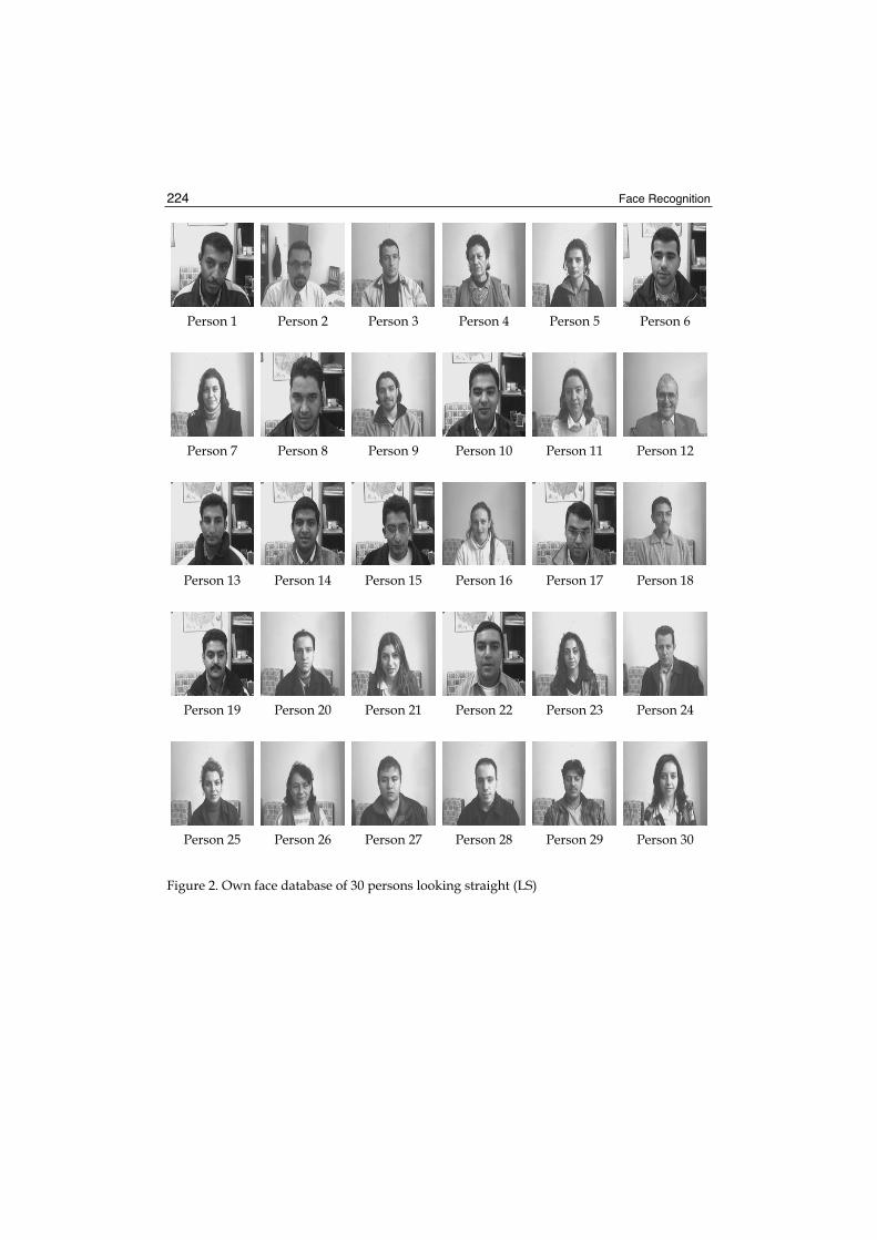
Face Recognition 224
Person 1 Person 2 Person 3 Person 4 Person 5 Person 6
Person 7 Person 8 Person 9 Person 10 Person 11 Person 12
Person 13 Person 14 Person 15 Person 16 Person 17 Person 18
Person 19 Person 20 Person 21 Person 22 Person 23 Person 24
Person 25 Person 26 Person 27 Person 28 Person 29 Person 30
Figure 2. Own face database of 30 persons looking straight (LS)

Intelligent Global Face Recognition 225
Person 1 Person 2 Person 3 Person 4 Person 5 Person 6
Person 7 Person 8 Person 9 Person 10 Person 11 Person 12
Person 13 Person 14 Person 15 Person 16 Person 17 Person 18
Person 19 Person 20 Person 21 Person 22 Person 23 Person 24
Person 25 Person 26 Person 27 Person 28 Person 29 Person 30
Figure 3. Own face database of 30 persons looking right (LR)

Face Recognition 226
Person 1 Person 2 Person 3 Person 4 Person 5 Person 6
Person 7 Person 8 Person 9 Person 10 Person 11 Person 12
Person 13 Person 14 Person 15 Person 16 Person 17 Person 18
Person 19 Person 20 Person 21 Person 22 Person 23 Person 24
Person 25 Person 26 Person 27 Person 28 Person 29 Person 30
Figure 4. Own face database of 30 persons looking left (LL)

Intelligent Global Face Recognition 227
4.3 Glance Simulation (Global Pattern Averaging)
The method used for presenting the images to the neural network is based on global pattern averaging, which provides the glance approximation. A face image of size 100x100 pixels is segmented and the values of the pixels within each segment are averaged. The result average values are then used as input data for the neural network. The averaging of the segments within an image reduces the amount of data required for neural network implementation thus providing a faster recognition system. This also provides flexible mathematical inputs for neural networks that simulate the quick glance of a human which is sufficient for pattern recognition. Global pattern averaging can be defined as follows:
( )= =
=l k
ilk
s
l
s
klkp
ssiPatAv1 1
,1 , (1)
where k and l are segment coordinates in the x and y directions respectively, i is the segment number, Sk and Sl are segment width and height respectively, Pi(k,l) is pixel value at coordinates k and l in segment i, PatAvi is the average value of pattern in segment i, that is presented to neural network input layer neuron i. The number of segments in each window (of size X*Y pixels) containing a face, as well as the number of neurons in the input layer is iwhere
i = -{0, 1, 2, …, n}, (2)
and
=lk sY
sXn . (3)
Segment size of 10x10 pixels (Sk = Sl = 10) has been used and average values representing the image were obtained, thus resulting in 100 average values in total (n = 100) that were used as the input to the neural network for both training and testing. Figure 5 shows an example of this pre-processing phase. The original 512x512 pixel image is reduced to 256x256 pixels and then to 128x128 pixels. This is followed by extracting a region of size 100x100 pixels that contains the face. The extracted region is then segmented (tiled) and averaged yielding a 10x10 pixel pattern that represents the original image.
Figure 5. Image pre-processing before neural network training or testing
Original Image Image Image Image Pattern (512x512) pixels (256x256) pixels (128x128) pixels (100x100) pixels (10x10)

Face Recognition 228
4.4 Familiarity Simulation (Neural Network Implementation)
The multilayer perceptron neural network, which was developed as part of this global face recognition system, is based on the back propagation learning algorithm, with a total number of three layers, comprising, input layer, hidden layer and output layer. The input layer has 100 neurons, each receiving an averaged value of the face image segments. The hidden layer consists of 99 neurons, whereas the output layer has 30 neurons according to the number of persons. Figure 6 shows the topology of this neural network and image data presentation to the input layer.
Figure 6. Global pattern averaging and neural network design
The approach within this case study is based on simulating the “glance” and “familiarity” of faces in humans. The glance effect is approximated via image pre-processing and global pattern averaging as described in (section 4.3), whereas, familiarity of a face is simulated by training the neural network using face images with different orientations. The implementation of a neural network consists of training and testing. In this work a total of 90 face images (corresponding to 30 persons) were used. For training the neural network 60 face images (looking left LL and looking right LR) were used. The 30 remaining face images (looking straight LS) were used for testing purposes where the system is expected to recognize the person looking straight at the camera by training it on face images looking left and right. This simulates the familiarity of a face in machines, even though the test images (looking straight) present a neural network with different pixel values as a result of the difference in the orientation of the face. A recognition system “sensitivity” feature was also developed as part of the neural network classification of input face images. Three levels of tolerance, namely Low (minimum 80% face resemblance), Medium (minimum 65% face resemblance) or High (minimum 50% face resemblance) can be used depending on the required level of accuracy. The results that are presented in the next section were obtained using Low tolerance (i.e. minimum 80% face resemblance).
1
Original Image (512x512) pixels
Input Layer
Averaged Image (10x10) pixels
30
2
3
98
99
100
1
2
99
Hidden Layer
Output Layer
1 PERSON
2

Intelligent Global Face Recognition 229
5. Results and Discussion
The back propagation neural network, within the intelligent system, learnt and converged after 4314 iterations and within 390 seconds, whereas the running time for the trained neural network after training and using one forward pass was 0.21 seconds. These time cost results were obtained using the following system configuration: 2.4 GHz PC with 256 MB of RAM using Windows XP operating system, C-language source code and Borland C++ compiler. Table 1 lists the final parameters of the successfully trained neural network. All training images (60 face images- looking left and right) were correctly recognized when used for testing the trained neural network yielding 100% recognition rate as would be expected. The recognition of the testing face images (30 face images – looking straight) indicates the success and robustness of this intelligent system, as these face images had not been presented to the neural network before. Additionally, the “look straight” face images have different orientation and, thus, different pixel values in comparison to the training face images “look left” and “look right” at similar coordinates. Testing the neural network using these different test images yielded a successful 96.67% recognition rate where 29 out of 30 faces were correctly identified.
Input Layer Nodes 100 Hidden Layer Nodes 99 Output Layer Nodes 30 Bias Neurons Value 1 Learning Rate 0.008 Momentum Rate 0.32 Minimum Error 0.002 Initial Random Weights Range -0.3 to +0.3 Iterations 4314 Training Time (seconds) 390 Generalization/Run Time (seconds) 0.21
Table 1. Trained neural network final parameters using global face data
Figure 7. Incorrect identification of Person 23 as person 21
Person 23 Person 21
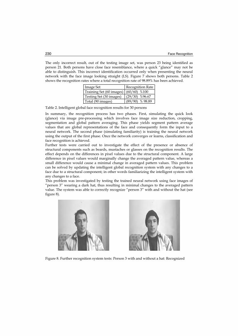
Face Recognition 230
The only incorrect result, out of the testing image set, was person 23 being identified as person 21. Both persons have close face resemblance, where a quick “glance” may not be able to distinguish. This incorrect identification occurred only when presenting the neural network with the face image looking straight (LS). Figure 7 shows both persons. Table 2 shows the recognition rates where a total recognition rate of 98.89% has been achieved.
Image Set Recognition RateTraining Set (60 images) (60/60) %100 Testing Set (30 images) (29/30) %96.67 Total (90 images) (89/90) % 98.89
Table 2. Intelligent global face recognition results for 30 persons
In summary, the recognition process has two phases. First, simulating the quick look (glance) via image pre-processing which involves face image size reduction, cropping, segmentation and global pattern averaging. This phase yields segment pattern average values that are global representations of the face and consequently form the input to a neural network. The second phase (simulating familiarity) is training the neural network using the output of the first phase. Once the network converges or learns, classification and face recognition is achieved. Further tests were carried out to investigate the effect of the presence or absence of structural components such as beards, mustaches or glasses on the recognition results. The effect depends on the differences in pixel values due to the structural component. A large difference in pixel values would marginally change the averaged pattern value, whereas a small difference would cause a minimal change in averaged pattern values. This problem can be solved by updating the intelligent global recognition system with any changes to a face due to a structural component; in other words familiarizing the intelligent system with any changes to a face. This problem was investigated by testing the trained neural network using face images of “person 3” wearing a dark hat, thus resulting in minimal changes to the averaged pattern value. The system was able to correctly recognize “person 3” with and without the hat (see figure 8).
Figure 8. Further recognition system tests: Person 3 with and without a hat: Recognized
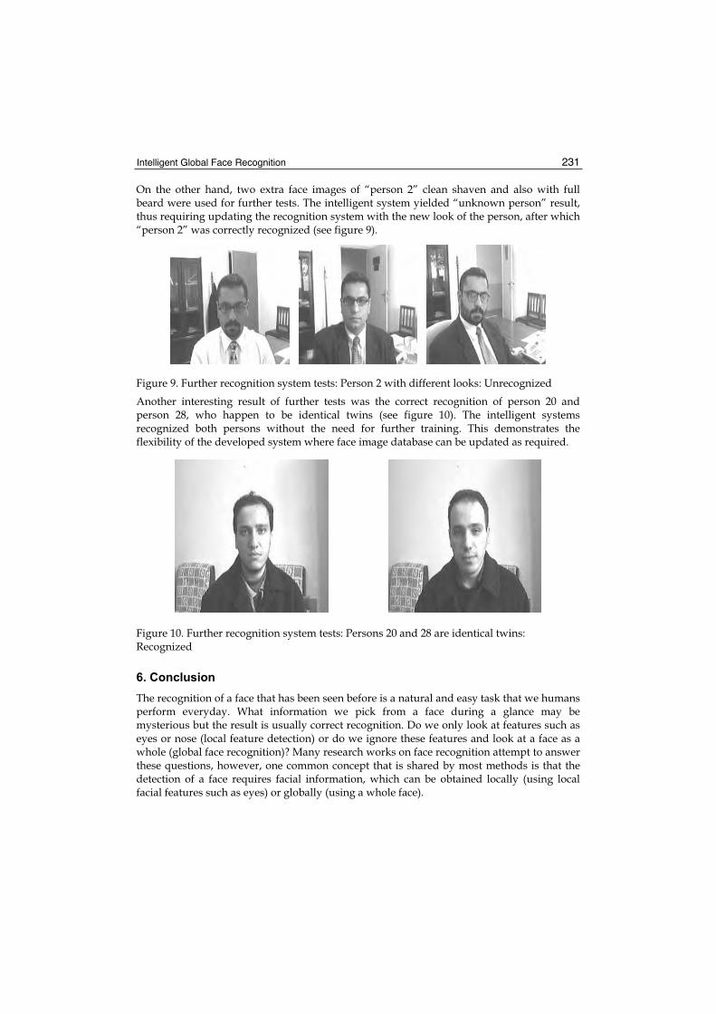
Intelligent Global Face Recognition 231
On the other hand, two extra face images of “person 2” clean shaven and also with full beard were used for further tests. The intelligent system yielded “unknown person” result, thus requiring updating the recognition system with the new look of the person, after which “person 2” was correctly recognized (see figure 9).
Figure 9. Further recognition system tests: Person 2 with different looks: Unrecognized
Another interesting result of further tests was the correct recognition of person 20 and person 28, who happen to be identical twins (see figure 10). The intelligent systems recognized both persons without the need for further training. This demonstrates the flexibility of the developed system where face image database can be updated as required.
Figure 10. Further recognition system tests: Persons 20 and 28 are identical twins: Recognized
6. Conclusion
The recognition of a face that has been seen before is a natural and easy task that we humans perform everyday. What information we pick from a face during a glance may be mysterious but the result is usually correct recognition. Do we only look at features such as eyes or nose (local feature detection) or do we ignore these features and look at a face as a whole (global face recognition)? Many research works on face recognition attempt to answer these questions, however, one common concept that is shared by most methods is that the detection of a face requires facial information, which can be obtained locally (using local facial features such as eyes) or globally (using a whole face).

Face Recognition 232
The diversity of the different methods and approaches is more evident when investigating the development of artificially intelligent face recognition systems. These intelligent systems aim to simulate the way we humans recognize faces, and the methods that are developed to achieve such an aim are as diverse as our natural individual perception of faces. This chapter presented a review of related works on face recognition in general and on intelligent global face recognition in particular. The presented case study is based on using global (complete face and background) data averaging and a neural network in order to simulate the human “glance” and face “familiarity”. The glance effect is approximated via image pre-processing and global pattern averaging. When we humans have a quick look (glance) at faces, we do not observe the detailed features but rather a general global impression of a face. This can be approximated by averaging the face image instead of searching for features within the face. The averaged patterns are representation of a face regardless of its expression or orientation. The quick glance is followed by familiarity with a face, which is simulated by training a neural network using face images with different orientations. The neural network within the intelligent system learnt to classify the faces within 390 seconds, whereas the running time for the trained neural network was 0.21 seconds. These time costs can be further reduced by using faster machines, which will inevitably occur in the near future. The implementation of the intelligent global face recognition system used 90 face images of 30 persons of different gender, age and ethnicity. A total recognition rate of 98.89% was obtained using 90 face images (combining training and testing images) of the 30 persons in different orientations. Only one person’s face image (looking straight) was mistaken for another person (looking straight too) as shown in Figure 7. The robustness and success of this face recognition system was further demonstrated by its quick run time (one neural network forward pass) of 0.21 seconds. Time cost was kept minimal through image-pre-processing and reduction of input/hidden layer neurons in the topology of the neural network. Further tests of the trained neural network within the intelligent system investigated the effects of the presence or absence of structural components such as beards or hats on the recognition results. The outcome of these tests suggests that some of the “familiar” faces may not be recognized if there is a drastic change on the face, this is due to the large difference in pixel values which would marginally change the averaged global pattern values. On the other hand, a small difference would cause a minimal change in averaged global pattern values, and thus would not affect the recognition results. This problem can be solved by updating the intelligent global recognition system with any changes to a face due to a structural component; in other words familiarizing the intelligent system with the new look of a person. Additionally, three levels of tolerance can be used when implementing the system that was presented in the case study. The choice of the tolerance level depends on the required level of accuracy: low tolerance (80% face resemblance), medium tolerance (65% face resemblance) or high tolerance (50% face resemblance). All results that were shown in the case study on intelligent global face recognition were obtained using the low tolerance classification, where a minimum of 80% face resemblance was required. This is believed to be a good resemblance ratio considering the neural network is trained using globally averaged patterns of faces and backgrounds.

Intelligent Global Face Recognition 233
Further work on intelligent global face recognition will investigate the acquisition of facial data using only left and right portfolios of a face. The developed neural network for this task would use different parameters obtained using other methods (e.g. edge detection) in order to associate the face with the person. Finally, despite successful implementations of artificial intelligent face recognition systems such as our case study, there are questions that are yet to be answered before we can completely trust a machine whose intelligence “evolves” in minutes in comparison with our natural intelligence that took thousands of years to evolve. There is no doubt that the advancement in technology provides us with the means to develop efficient artificially intelligent systems, however, the question remains: how intelligent are they really are?
7. References
Belhumeur, P.N. ; Hespanha, J.P. & Kriegman, D.J. (1997). Eigenfaces vs. Fisherfaces: Recognition Using Class Specific Linear Projection, IEEE Transactions (PAMI), Vol. 19, No. 7, (1997), (711-720)
Fan, X. & Verma, B. (2005). A Comparative Experimental Analysis of Separate and Combined Facial Features for GA-ANN based Technique, Proceedings of Conference on Computational Intelligence and Multimedia Applications, pp. 279-284
He, X. & Niyogi, P. (2003). Locality Preserving Projections, Proceedings of Conference on Advances in Neural Information Processing Systems
He, X. ; Yan, S. ; Hu, Y. ; Niyogi, P. & Zhang, H.J. (2005). Face Recognition Using Laplacianfaces, IEEE Transactions (PAMI), Vol. 27, No. 3, (2005), (328-340)
Huang, L.L. & Shimizu, A. (2006). Combining Classifiers for Robust Face Detection. In Lecture Notes in Computer Science, (116-121), 3972, Springer-Verlag
Khashman, A. (2006). Face Recognition Using Neural Networks and Pattern Averaging, In Lecture Notes in Computer Science, (98–103), 3972, Springer-Verlag
Levin, A. & Shashua, A. (2002). Principal Component Analysis over Continuous Subspaces and Intersection of Half-Spaces, In Proceedings of European Conf. Computer Vision.Vol. 3, (2002), pp. 635-650
Li, G. ; Zhang, J. ; Wang, Y. & Freeman, W.J. (2006). Face Recognition Using a Neural Network Simulating Olfactory Systems. In Lecture Notes in Computer Science, (93-97), 3972, Springer-Verlag
Li, S.Z. ; Hou, X.W. ; Zhang, H.J. & Cheng, Q.S. (2001). Learning Spatially Localized, Parts-Based Representation. In Proceedings of IEEE Conf. Computer Vision and Pattern Recognition, pp. 207-212
Li, S.Z. & Jain, A.K. (2005). Handbook Of Face Recognition, Springer-Verlag Lu, K. ; He, X. & Zhao, J. (2006). Semi-supervised Support Vector Learning for Face
Recognition. In Lecture Notes in Computer Science, (104-109), 3972, Springer-Verlag Lu, X. ; Wang, Y. & Jain, A.K. (2003). Combining Classifiers for Face Recognition, In IEEE
Conference on Multimedia & Expo, Vol. 3, pp. 13-16 Martinez, A.M. & Kak, A.C. (2001). PCA versus LDA. In IEEE Transactions (PAMI), Vol. 23,
No. 2, (2001), (228-233) Murase, H. & Nayar, S.K. (1995). Visual Learning and Recognition of 3-D Objects from
Appearance. In Journal of Computer Vision, Vol. 14, (1995), (5-24)

Face Recognition 234
Pang, S. ; Kim, D. & Bang, S.Y. (2005). Face Membership Authentication Using SVM Classification Tree Generated by Membership-Based LLE Data Partition. In IEEE Transactions on Neural Networks, Vol. 16, No. 2, (2005), (436-446)
Park, C. ; Ki, M. ; Namkung, J. & Paik, J.K. (2006). Multimodal Priority Verification of Face and Speech Using Momentum Back-Propagation Neural Network. In Lecture Notes in Computer Science, (140-149), 3972, Springer-Verlag
Roweis, S.T. & Saul, L.K. (2000). Nonlinear Dimensionality Reduction by Locally Linear Embedding. In Science, No. 290, (2323-2326)
Turk, M. & Pentland, A.P. (1991). Face Recognition Using Eigenfaces, In Proceedings of IEEE Conference on Computer Vision and Pattern Recognition, pp. 586-591
Yang, M.H. ; Kriegman, D.J. & Ahuja, N. (2002). Detecting Faces in Images: A Survey. In IEEE Transactions (PAMI), Vol. 24, No. 1, (2002), (34-58)
Zhang, B. ; Zhang, H. & Ge, S. (2004). Face Recognition by Applying Wavelet Subband Representation and Kernel Associative Memory. In IEEE Transactions on Neural Networks, Vol.15, (2004), (166-177)
Zhou, W. ; Pu, X. & Zheng, Z. (2006). Parts-Based Holistic Face Recognition with RBF Neural Networks. In Lecture Notes in Computer Science, (110-115), 3972, Springer-Verlag

12
Compact Parallel Optical Correlator for Face Recognition, and Its Application
Kashiko Kodate and Eriko Watanabe Faculty of Science, Japan Women’s University
Japan
1. Introduction
With the ongoing progress in information technology, the need for an accurate personal identification system based on recognizing biological characteristics is increasing demand for this type of security technology, rather than conventional systems that use ID cards or pin numbers. Of all physical features, the face is the most familiar and recognizable, and using it for identification purposes avoids the need for physical contact, thereby also avoiding potential psychological or physical resistance, such as that encountered when trying to obtain fingerprints for example. Face recognition has been studied since the 1970s, with extensive research into and development of the digital processing of facial images. A range of software is already on the market. As a simple and compact recognition system that satisfies the required performance levels, we have implemented a hybrid system based on the optical recognition principle, using a Fourier transform lens. In contrast to digital recognition, optical analog operations process two-dimensional images instantaneously in parallel using a lens-based Fourier transform function (Kodate Hashimoto, & Thapliya, 1999). In the 1960s, two methods were proposed; the VanderLugt Correlator proposed by VanderLugt ((a)Watanabe & Kodate, 2005), and the joint transform correlator (JTC) ( Kodate Inaba & Watanabe, 2002) by Weaver and Goodman. The optical correlator by the Institut national d’Optique in Canada gained the New Product Award at the 1999 Conference on lasers and Electro-optics and the Quantum Electronics and Laser Science Conference. In Japan the conventional JTC was practically implemented by the Hamamatsu Photonics Company for fingerprint image processing. The process speed of optical correlators has steadily improved, however, operational speed, practicality and recognition rate were not fully tested against the fast-improving digitized system. Against this background, the present group of authors has proposed a new scheme using a multi-beam, multi-channel parallel joint transform correlator (PJTC) as a means of making better use of spatial parallelism through the use of a diffraction-type multi-level zone-plate array (MLZP array) to extend a single channel JTC ((b)Watanabe & Kodate , 2005). Watanabe & Kodate , 2003). Features of the proposed system include extreme robustness, high recognition precision by its pre-processing and high reproducibility by its post-process. The compact and mobile versions are now assembled and named COPaC. Specifications: 20x24x43 cm 3.6 kg, analysis time of 6.6 faces/s ( Kodate Inaba& Watanabe, 2002).

Face Recognition 236
In an attempt to downsize the hard disk, LD is replaced as a light source with a multi-light source module constructed by vertical cavity surface emitting laser (VCSEL) array and MLZPA. In spite of the constraints of the Fourier-transform type process, the speed of an optically controlled, liquid crystal spatial light modulator was accelerated to 30 ms. It is very difficult to achieve optical correlation speeds shorter than 30 ms. In recent years, devices for optical information processing have been developed. Examples include Ferroelectrics liquid crystal special light modulator (FLC-SLM) and digital micromirror device (DMD) which can enhance the high-speed display (1 kHz-10 kHz), and herald the possibility of accelerating the systemic processing time. Furthermore, a novel holographic optical storage system that utilizes co-axial holography was demonstrated. The VLC is conducive to improvements in speed, given that it can dispense with the optically addressed SLM. In practice, however, comprehensive system design and implementation should be required to make the most of the theoretical potential. We implemented a fully automatic FARCO (dimensions: 33.0x30.5x17.8 cm³) ((a)Watanabe & Kodate, 2005), which achieved an operation speed of more than 4000 faces/s using four-channel processing. The correlation filter we used was more accurate than various correlation methods ((b)Watanabe & Kodate, 2005). Based on trial 1:N identification, FARCO achieved low error rates of 1% False acceptance rate (FAR) and 2.3% false rejection rate (FRR). The recognition time of FARCO is limited to about 1,000frame/s due to the date transfer speed and storage capacity of the random access memory (RAM) used to store digital reference images. The time of data transfer speed is converted from the digital data to optical image data in the optical system. Using the ability of parallel transformation as optical holographic memory, the recognition rate can be vastly improved. In addition, a large optical storage capacity allows us to increase the size of the reference database. A novel holographic optical storage system that utilizes co-axial holography has recently been demonstrated (Horimai & Tan, 2006). This process can produce a practical and small holographic optical storage system more easily than conventional off-Coaxial holographic system. At present, the system seems to be most promising for ultra high density volumetric optical storage In this chapter, we present the compact optical parallel correlator for face recognition, and its application. This is a product of lengthy processes, and long-term efforts to overcome several obstacles such as attaining precision in the optical correlation system, operational speed and downsizing. Crucial technologies applied in the system include our unique and extremely precise phase filter and high-speed optical devices that we have been perfecting over many years. Combined with these, a novel system structure and algorithm were proposed and tested in rigorous experiments. Section 2 addresses the basic principle of optical pattern recognition by optical Fourier transform and the importance of phase information in face image. In Section 3, the concept of an optical correlation system for facial recognition and dedicated algorithm is presented. Section 4 provides the design of the correlation filter and an evaluation and comparison of the correlation filters for FARCO, and also tests for evaluating the recognition system, and experimental results of 1:N identifications and so on. A highly precise algorithm using multiple database images for FARCO is introduced in Section 5. A constructed 3 dimentional (3-D) face model is discussed in Section 6. In Section 7, a high security facial recognition system using a cellular phone is presented. A super high-speed optical correlator that integrates an optical correlation technology used in FARCO (fast face-recognition optical correlator) and co-axial

Compact Parallel Optical Correlator for Face Recognition, and Its Application 237
holographic storage system is proposed. Section 9 discusses the future works and Section 10 concludes the chapter.
2. The Basic Principle of Optical Correlation
The optical implementation of pattern recognition can be accomplished with either Fourier domain complex matched filtering or spatial domain filtering. Correlators that use Fourier domain matched filtering are commonly known as VLC’s. The basic distinctions between them are that the VLC depends on Fourier-domain spatial filter synthesis (e.g., Fourier hologram). In other words the complex spatial detection of the VanderLugt arrangement is input scene independent. The basic optical setup of the VLC type of correlator is depicted in Fig. 1. A prefabricated Fourier-domain matched filter H (u,v) is needed in the VLC. This section describes the basic principle optical pattern recognition by optical Fourier transform. We also address the importance of phase information in the face image. Optical correlation is one pattern-matching method used for finding whether there is a correlation between images in the database and input images, using analogue calculation based on the parallelism of light. In this method, all the information of the images can be searched at the speed of light, to determine whether the images belong to the same person. The principle of optical setup was designed for Fourier-domain matched filter, which was applied to our face recognition system. Let us consider a thin convex lens of focal length f, illuminated by a laser beam. Output facial images set in the real space are Fourier-transformed in the spatial frequency plane. The complex conjugate of this Fourier-transformed image is stored in a matched filter, which is then to be positioned at the optical devices (Fig.1 (b)) and Fourier-transformed again. On the output plane, the correlation term and convolution term will be displayed. For a more detailed description of this setup, please refer to precedent literature (Goodman & Moeller, 2004. Hecht, 1998). This section describes the basic principle optical pattern recognition by optical Fourier transform. We also address the importance of phase information in the face image.
2.1 Importance of Phase Information
As shown in Fig. 2, 2-dimensional images in real space have amplitude information, which can be singled out by Fourier transformation into amplitude and phase information in spectrum space. The phase image is defined using absolute values of distribution. Where F is Fourier operator, where F (u, v) is phase distribution.
F(u,v) = | F(u, v)|exp[-j F(u,v)] (1)
Images, of which only phase was Fourier-transformed, can be defined by the following equation.
f (x,y) = F -1{( u,v)|exp[-j F(u,v)]} (2)
The intensity of the object is represented by amplitude F(u,v), while its phase information is displayed by F(u,v).
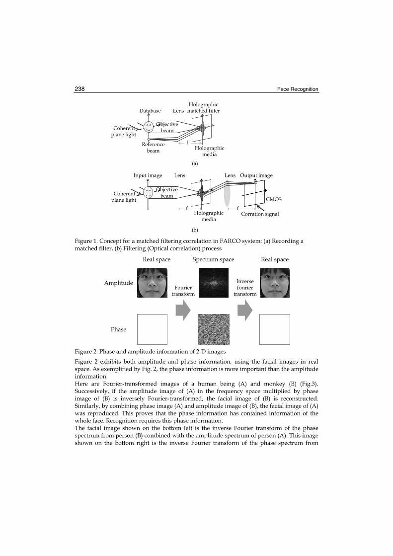
Face Recognition 238
Lens
LensLens
(a)
Database
ff
Coherentplane light
Coherentplane light
Holographicmatched filter
Corration signal
Objectivebeam
Objectivebeam
Input image Output image
Referencebeam Holographic
media
Holographicmedia
CMOS
f
(b)
Figure 1. Concept for a matched filtering correlation in FARCO system: (a) Recording a matched filter, (b) Filtering (Optical correlation) process
Real space Spectrum space
Fouriertransform
Inversefourier
transform
Real space
Phase
Amplitude
Figure 2. Phase and amplitude information of 2-D images
Figure 2 exhibits both amplitude and phase information, using the facial images in real space. As exemplified by Fig. 2, the phase information is more important than the amplitude information. Here are Fourier-transformed images of a human being (A) and monkey (B) (Fig.3). Successively, if the amplitude image of (A) in the frequency space multiplied by phase image of (B) is inversely Fourier-transformed, the facial image of (B) is reconstructed. Similarly, by combining phase image (A) and amplitude image of (B), the facial image of (A)was reproduced. This proves that the phase information has contained information of the whole face. Recognition requires this phase information. The facial image shown on the bottom left is the inverse Fourier transform of the phase spectrum from person (B) combined with the amplitude spectrum of person (A). This image shown on the bottom right is the inverse Fourier transform of the phase spectrum from
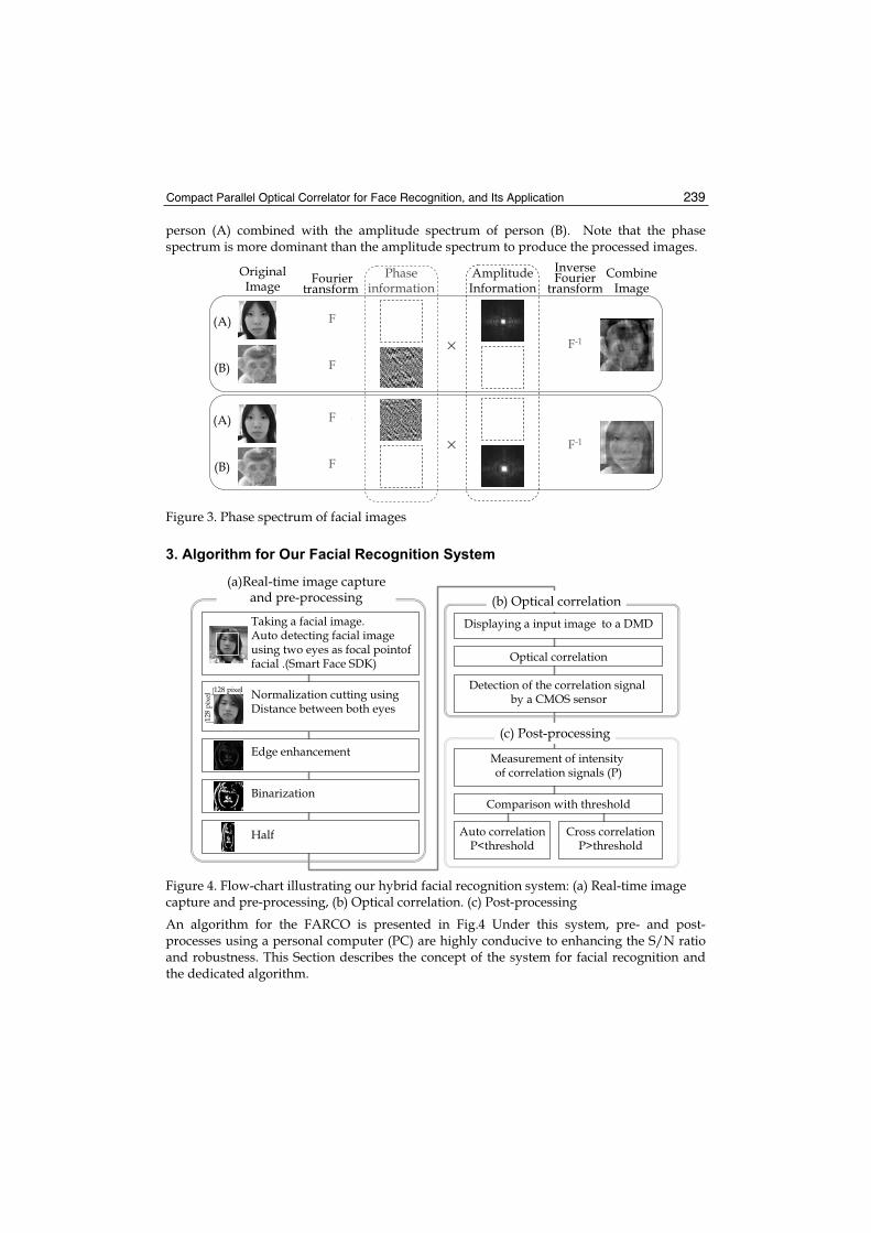
Compact Parallel Optical Correlator for Face Recognition, and Its Application 239
person (A) combined with the amplitude spectrum of person (B). Note that the phase spectrum is more dominant than the amplitude spectrum to produce the processed images.
F
FF-1
F
F
F-1
(A)
(A)
(B)
(B)
AmplitudeInformation
Phaseinformation
OriginalImage Fourier
transform
InverseFourier
transform Combine
Image
Figure 3. Phase spectrum of facial images
3. Algorithm for Our Facial Recognition System
Auto correlationP<threshold
128 pixel
128
pixe
l 128 pixel
128
pixe
l
Taking a facial image.Auto detecting facial image using two eyes as focal pointoffacial .(Smart Face SDK)
Displaying a input image to a DMD
Detection of the correlation signal by a CMOS sensor
Optical correlation
Measurement of intensity of correlation signals (P)
Comparison with threshold
Cross correlationP>threshold
Normalization cutting using Distance between both eyes
Edge enhancement
Binarization
Half
(a)Real-time image capture and pre-processing (b) Optical correlation
(c) Post-processing
Figure 4. Flow-chart illustrating our hybrid facial recognition system: (a) Real-time image capture and pre-processing, (b) Optical correlation. (c) Post-processing
An algorithm for the FARCO is presented in Fig.4 Under this system, pre- and post- processes using a personal computer (PC) are highly conducive to enhancing the S/N ratio and robustness. This Section describes the concept of the system for facial recognition and the dedicated algorithm.
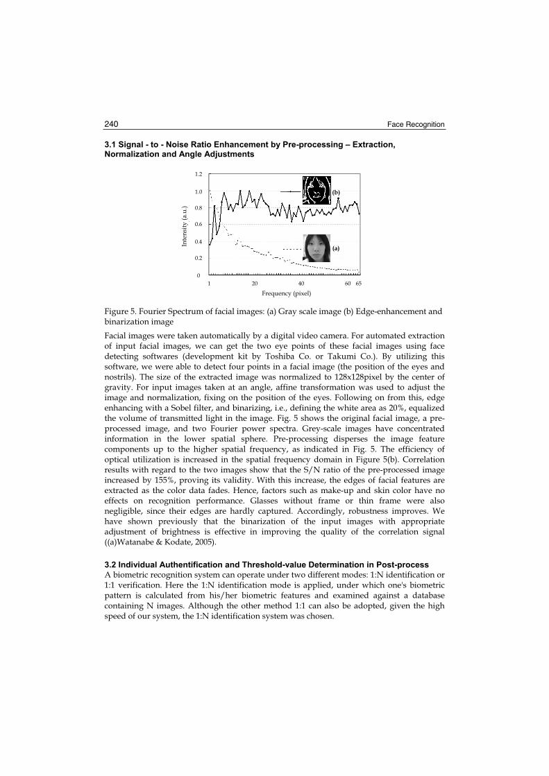
Face Recognition 240
3.1 Signal - to - Noise Ratio Enhancement by Pre-processing – Extraction, Normalization and Angle Adjustments
1 20 40 60 65
Frequency (pixel)
Inte
nsity
(a.u
.)
0
0.2
0.4
0.6
0.8
1.0
1.2
(a)
(b)
Figure 5. Fourier Spectrum of facial images: (a) Gray scale image (b) Edge-enhancement and binarization image
Facial images were taken automatically by a digital video camera. For automated extraction of input facial images, we can get the two eye points of these facial images using face detecting softwares (development kit by Toshiba Co. or Takumi Co.). By utilizing this software, we were able to detect four points in a facial image (the position of the eyes and nostrils). The size of the extracted image was normalized to 128x128pixel by the center of gravity. For input images taken at an angle, affine transformation was used to adjust the image and normalization, fixing on the position of the eyes. Following on from this, edge enhancing with a Sobel filter, and binarizing, i.e., defining the white area as 20%, equalized the volume of transmitted light in the image. Fig. 5 shows the original facial image, a pre-processed image, and two Fourier power spectra. Grey-scale images have concentrated information in the lower spatial sphere. Pre-processing disperses the image feature components up to the higher spatial frequency, as indicated in Fig. 5. The efficiency of optical utilization is increased in the spatial frequency domain in Figure 5(b). Correlation results with regard to the two images show that the S/N ratio of the pre-processed image increased by 155%, proving its validity. With this increase, the edges of facial features are extracted as the color data fades. Hence, factors such as make-up and skin color have no effects on recognition performance. Glasses without frame or thin frame were also negligible, since their edges are hardly captured. Accordingly, robustness improves. We have shown previously that the binarization of the input images with appropriate adjustment of brightness is effective in improving the quality of the correlation signal ((a)Watanabe & Kodate, 2005).
3.2 Individual Authentification and Threshold-value Determination in Post-process
A biometric recognition system can operate under two different modes: 1:N identification or 1:1 verification. Here the 1:N identification mode is applied, under which one's biometric pattern is calculated from his/her biometric features and examined against a database containing N images. Although the other method 1:1 can also be adopted, given the high speed of our system, the 1:N identification system was chosen.

Compact Parallel Optical Correlator for Face Recognition, and Its Application 241
The False Acceptance Rate denotes the probability that a biometric system will incorrectly identify an individual, or will fail to reject an impostor. For a positive (verification) system, it can be estimated from: (the number of false acceptances) / (the number of impostor verification attempts). Conversely, False Rejection Rate (FRR) is the probability that a biometric system will not identify an individual, or will fail to accept a person in the database. For a positive (verification) system, it can be estimated from: (the number of false rejections) / (the number of times it fails to verify). In practical application, the threshold value has to be customized by the application. The threshold value varies with its security level; depending on whether the system is designed to reject an unregistered person or permitting at least one registered person. We have to decide the optimum threshold value using the appropriate number of database images based on the biometrics guideline for each application. In this paper, the threshold value is fixed where FRR and FAR are lowest. We determined the sample number was according to the definition of one of the accuracy evaluation authorities, National Biometric Test Center (Japan). The error margin P in the sample number N was given by the following equation, under the reliability 95%.
N = 3/P (3)
For example, where P=0.01, 300 samples (i.e. persons) are required. The sample number determined was 300 persons; the facial images of 240 women (20-50 years old) were taken on the same day, while images of 60 men were pre-processed. One hundred and fifty were registered, while the second half was unregistered. The correlation value (where i is the entry number of test image and j is the reference number) is stored in a memory and the maximum value, Pi mCoaxial searched. Then, all the correlation values are normalized by Pi max.Here, we define the comparison value, which is used as threshold for 1:N identification, Ci by Equation(4). (Inaba Kodate & Watanabe, 2003)
Ci = Pij/Pimax–1/(N – 1) (4)
Using the devised correlation filters, simulation experiments were conducted under the assumption of 1:N identification.
4. Fast Face-Recognition Optical Correlator
We have developed a face recognition system named FARCO, which has three different configurations depending on its recognition rate shown in Fig.6. This is an improvement on one-to-one ID recognition system, which requires little calculation time. The FARCO system is a hybrid optical correlator that integrates an optical correlation technology and digital database. FARCO can be applied to several hundreds of images, with its operation speed of 1000 to 5000 faces per second. In order to correspond to greater demand, the S-FARCO (Super fast face-recognition optical correlator) system is used. The S-FARCO is equipped with a holographic optical memory, which could store and process information optically. This enables optical correlation without decoding information in the database, which greatly reduces processing time (more details in Section 8). This Section will present the correlation filter, its optical setup and experimental results focus on FARCO.
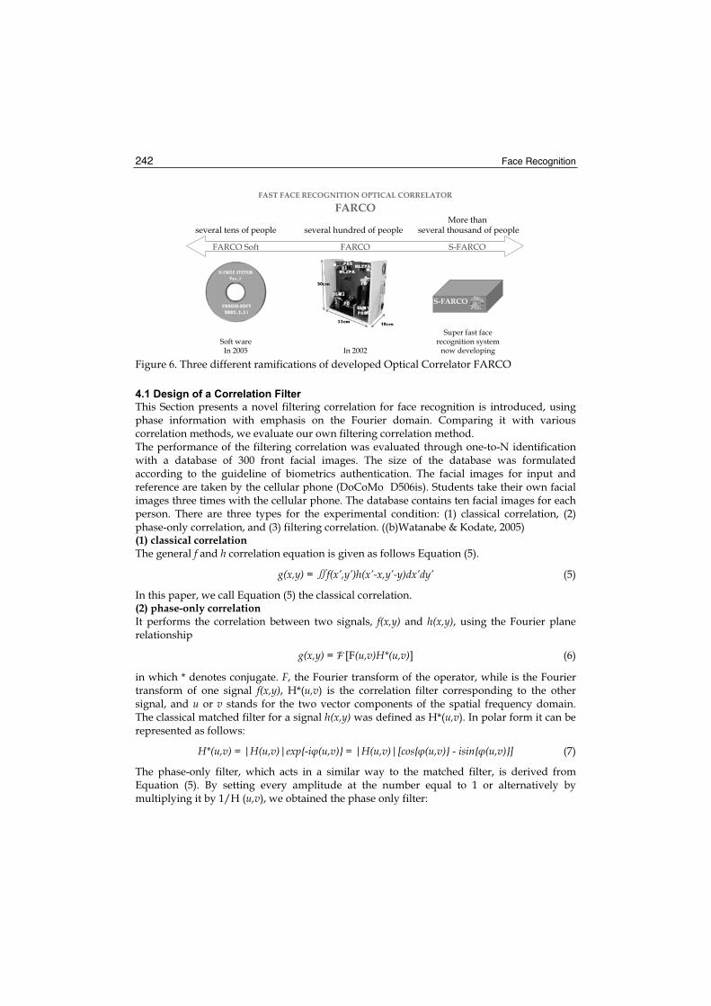
Face Recognition 242
several tens of people
Soft wareIn 2005
FARCO
In 2002
S-FARCO
FAST FACE RECOGNITION OPTICAL CORRELATOR
FARCO
several hundred of peopleMore than
several thousand of people
Super fast facerecognition system
now developing
FARCO Soft
S-FARCO
Figure 6. Three different ramifications of developed Optical Correlator FARCO
4.1 Design of a Correlation Filter
This Section presents a novel filtering correlation for face recognition is introduced, using phase information with emphasis on the Fourier domain. Comparing it with various correlation methods, we evaluate our own filtering correlation method. The performance of the filtering correlation was evaluated through one-to-N identification with a database of 300 front facial images. The size of the database was formulated according to the guideline of biometrics authentication. The facial images for input and reference are taken by the cellular phone (DoCoMo D506is). Students take their own facial images three times with the cellular phone. The database contains ten facial images for each person. There are three types for the experimental condition: (1) classical correlation, (2) phase-only correlation, and (3) filtering correlation. ((b)Watanabe & Kodate, 2005) (1) classical correlation The general f and h correlation equation is given as follows Equation (5).
g(x,y) = f(x’,y’)h(x’-x,y’-y)dx’dy’ (5)
In this paper, we call Equation (5) the classical correlation. (2) phase-only correlation It performs the correlation between two signals, f(x,y) and h(x,y), using the Fourier plane relationship
g(x,y) = F [F(u,v)H*(u,v)] (6)
in which * denotes conjugate. F, the Fourier transform of the operator, while is the Fourier transform of one signal f(x,y), H*(u,v) is the correlation filter corresponding to the other signal, and u or v stands for the two vector components of the spatial frequency domain. The classical matched filter for a signal h(x,y) was defined as H*(u,v). In polar form it can be represented as follows:
H*(u,v) = |H(u,v)|exp{-i (u,v)} = |H(u,v)|[cos{ (u,v)} - isin{ (u,v)}] (7)
The phase-only filter, which acts in a similar way to the matched filter, is derived from Equation (5). By setting every amplitude at the number equal to 1 or alternatively by multiplying it by 1/H (u,v), we obtained the phase only filter:
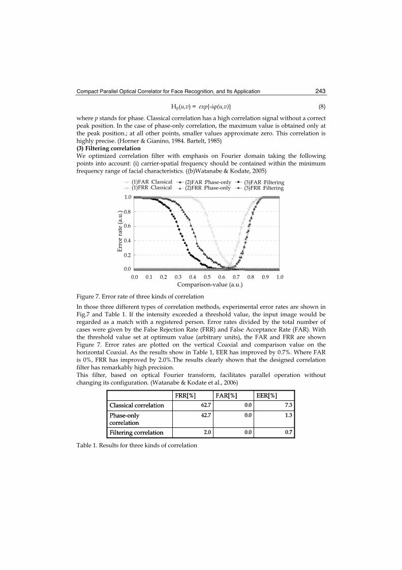
Compact Parallel Optical Correlator for Face Recognition, and Its Application 243
Hp(u,v) = exp{-i (u,v)} (8)
where p stands for phase. Classical correlation has a high correlation signal without a correct peak position. In the case of phase-only correlation, the maximum value is obtained only at the peak position.; at all other points, smaller values approximate zero. This correlation is highly precise. (Horner & Gianino, 1984. Bartelt, 1985) (3) Filtering correlation We optimized correlation filter with emphasis on Fourier domain taking the following points into account: (i) carrier-spatial frequency should be contained within the minimum frequency range of facial characteristics. ((b)Watanabe & Kodate, 2005)
(1)FAR Classical(1)FRR Classical
(2)FAR Phase-only(2)FRR Phase-only
(3)FAR Filtering(3)FRR Filtering
Comparison-value (a.u.)
Erro
r rat
e (a
.u.)
0.0 1.00.90.80.70.60.50.40.30.20.1
0.8
0.6
0.4
0.2
0.0
1.0
Figure 7. Error rate of three kinds of correlation
In those three different types of correlation methods, experimental error rates are shown in Fig.7 and Table 1. If the intensity exceeded a threshold value, the input image would be regarded as a match with a registered person. Error rates divided by the total number of cases were given by the False Rejection Rate (FRR) and False Acceptance Rate (FAR). With the threshold value set at optimum value (arbitrary units), the FAR and FRR are shown Figure 7. Error rates are plotted on the vertical Coaxial and comparison value on the horizontal Coaxial. As the results show in Table 1, EER has improved by 0.7%. Where FAR is 0%, FRR has improved by 2.0%.The results clearly shown that the designed correlation filter has remarkably high precision. This filter, based on optical Fourier transform, facilitates parallel operation without changing its configuration. (Watanabe & Kodate et al., 2006)
0.70.02.0Filtering correlation
1.30.042.7Phase-only correlation
7.30.062.7Classical correlationEER[%]FAR[%]FRR[%]
0.70.02.0Filtering correlation
1.30.042.7Phase-only correlation
7.30.062.7Classical correlationEER[%]FAR[%]FRR[%]
Table 1. Results for three kinds of correlation
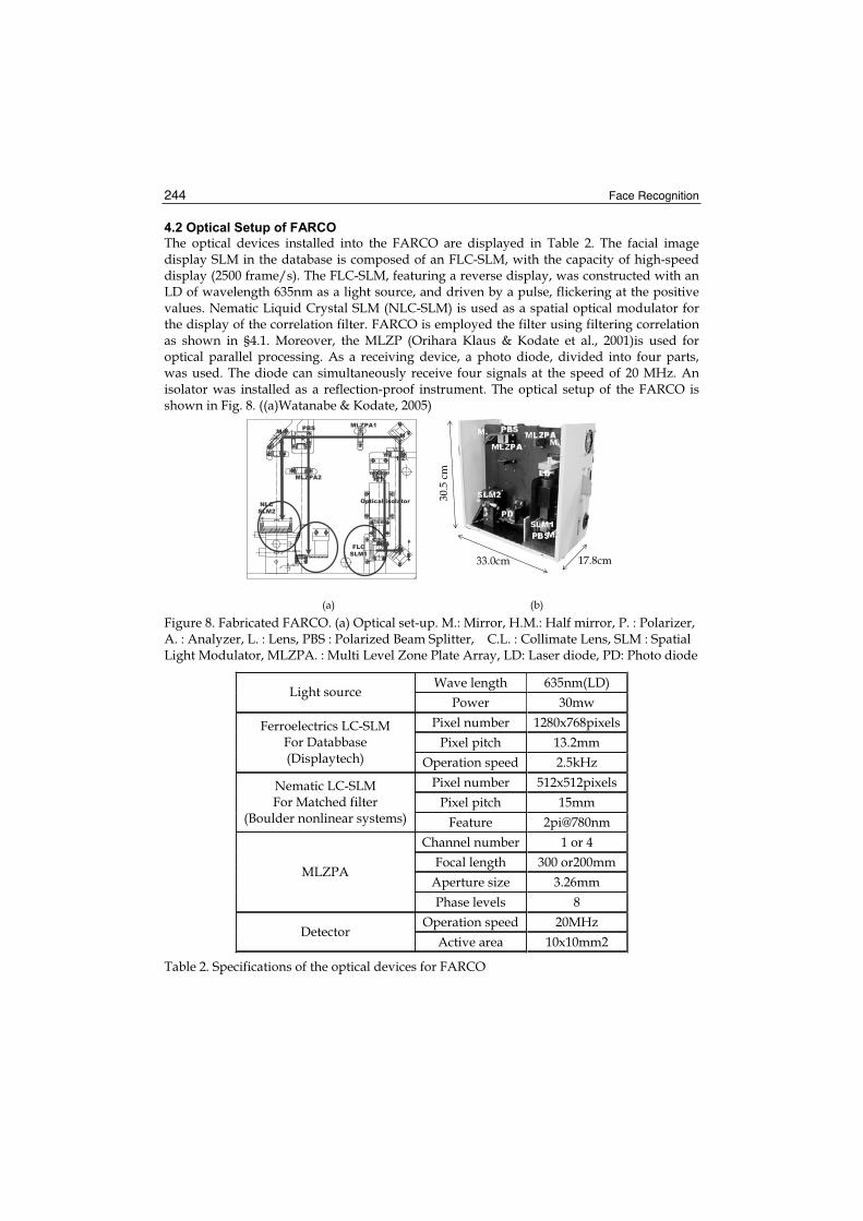
Face Recognition 244
4.2 Optical Setup of FARCO
The optical devices installed into the FARCO are displayed in Table 2. The facial image display SLM in the database is composed of an FLC-SLM, with the capacity of high-speed display (2500 frame/s). The FLC-SLM, featuring a reverse display, was constructed with an LD of wavelength 635nm as a light source, and driven by a pulse, flickering at the positive values. Nematic Liquid Crystal SLM (NLC-SLM) is used as a spatial optical modulator for the display of the correlation filter. FARCO is employed the filter using filtering correlation as shown in §4.1. Moreover, the MLZP (Orihara Klaus & Kodate et al., 2001)is used for optical parallel processing. As a receiving device, a photo diode, divided into four parts, was used. The diode can simultaneously receive four signals at the speed of 20 MHz. An isolator was installed as a reflection-proof instrument. The optical setup of the FARCO is shown in Fig. 8. ((a)Watanabe & Kodate, 2005)
33.0cm 17.8cm
30.5
cm
Optical isolator
FLCSLM1
NLCSLM2
MLZPA1
MLZPA2
PBS
PBS
1/2λ
M
MM
(a) (b)
Figure 8. Fabricated FARCO. (a) Optical set-up. M.: Mirror, H.M.: Half mirror, P. : Polarizer, A. : Analyzer, L. : Lens, PBS : Polarized Beam Splitter, C.L. : Collimate Lens, SLM : Spatial Light Modulator, MLZPA. : Multi Level Zone Plate Array, LD: Laser diode, PD: Photo diode
Wave length 635nm(LD) Light source
Power 30mw Pixel number 1280x768pixels
Pixel pitch 13.2mm Ferroelectrics LC-SLM
For Databbase (Displaytech) Operation speed 2.5kHz
Pixel number 512x512pixels Pixel pitch 15mm
Nematic LC-SLM For Matched filter
(Boulder nonlinear systems) Feature 2pi@780nm Channel number 1 or 4
Focal length 300 or200mm Aperture size 3.26mm
MLZPA
Phase levels 8 Operation speed 20MHz
DetectorActive area 10x10mm2
Table 2. Specifications of the optical devices for FARCO

Compact Parallel Optical Correlator for Face Recognition, and Its Application 245
4.3 Flowchart of FARCO System
A flow chart for optical correlation with the FARCO is presented in Fig. 9. Firstly, pre-processing was carried out within less than 200ms, covering the extraction of facial images through to the calculation of the correlation filter. On receiving final signals from the pre-process stage, NLC-SLM started up and showed the correlation filter obtained on the SLM in the correlator (see (2)-1 in Fig. 9). Initiated by the start-up signal from the NLC-SLM, the light pulse source begins to operate ((2)- 2, 3). Subsequently, the moment images in the database, stored in advance in an FLC-SLM board RAM of a control computer, are set for calculation, the instant correlation begins as each image is shown at the speed of 1000frame/s. Correlation signals through the filter were captured by a detector, and the recorded intensity is classified as a resemblance level ((2)- 4, 5). Each loop per optical correlation required 1 ms, although four parallel optical correlations with a parallel Fourier transform device, MLZP, only necessitate 4000 faces/s. In the final stage, post-processing the intensity values of these optical signals yielded final outcomes, i.e. recognition rates. In the case of the one-to-N identification experiment, Ci was calculated after N-loops, while values from every loop in the memory were recorded. Being used as an internal LAN on the university campus, this face recognition system is accessible to anyone with a camera and input software.
Figure 9. Flow chart of FARCO system
4.4 Experimental Results with FARCO
4.4.1 N identification with 4 channels
1:N identification experiments were conducted to examine the recognition performance of the FARCO, using the sample of 300 individual facial images. The FARCO system processes 1000 images per second by one channel. Thus it takes 0.15 seconds for the database with 150 registered person images. The ROC curve, acquired by the experiments with 4 channels, is shown in Fig. 10. This curve represents the FAR of 1.3% and the FRR of 2.6%, which is the lowest error rate of all with the FARCO. Relying on FAR values, the level of security system applicability varies. At the FAR below 1%, PC login and entry to communal houses are possible. With 1% FAR, FRR becomes 3.6%, which is within possible range of availability, in
1.Pre-Processing
2.Optical Correlator
(1)Displaying Filter image
Loop : j<N/channel
(2)Displaying the database image
(3)Optical Correlation
(4)Detecting correlation signals
(5)A/D converter
Loop : j<N/channel
3.Post-Processing
Trigsignal
Trigsignal

Face Recognition 246
compliance with the biometrics evaluation. Results of recognition experiments on a database containing over 4000 images are presented in Fig 11. This database has 80 people with 50 multiplex images per person. Operationalization at 4 ch enabled correlation with 4000 images.
0
1000
2000
1 51 101 151 201 251 301 351 401 451 501 551 601 651 701 751 801 851 901 951code number(a.u.)
corr
elat
ion inte
nsi
ty
(a.u
.)
0
1000
2000
1 51 101 151 201 251 301 351 401 451 501 551 601 651 701 751 801 851 901 951
code number(a.u.)
corr
elat
ion
inte
nsi
ty(a
.u.)
0
1000
2000
1 51 101 151 201 251 301 351 401 451 501 551 601 651 701 751 801 851 901 951code number(a.u.)
corr
elat
ion
inte
nsi
ty(a
.u.)
0
1000
2000
1 51 101 151 201 251 301 351 401 451 501 551 601 651 701 751 801 851 901 951 1001
code number(a.u.)
corr
elat
ion
iinte
nsi
tyl(a.
u.)
1ch
2ch
3ch
4ch
*
The sample of database images
Input image(code#1)
Registered number area of input image
(a)
(b)
correlation
Figure 10. Evaluation accuracy of FARCO according to the biometrics guideline with database images of 300 persons. The lowest error rates of the two values were recorded for 300 data, with FAR and FRR error rates of less than 1.3% and 2.6% respectively
0.001
0.01
0.1
1
0.001 0.01 0.1 1
FRR(a.u.)
FA
R(a
.u.)
FRR (a.u.)
FAR
(a.u
.)
0.001 10.01 0.1
0.001
0.01
0.1
1
Figure 11. Evaluation accuracy of FARCO according to biometrics guidline using 300 people database images

Compact Parallel Optical Correlator for Face Recognition, and Its Application 247
4.4.2 10 channel Experiment Results
We examined the correlation using multi-object reference images. When the correlation filter is applied to multi-object images, there are problems in that optical intensity is reflected by transmission intensity and diffraction angles. By using all 1280x768 pixels of SLM pixels, we can implement parallel operations of more than 10 channels. In this experiment, however, we designed and performed experiments limited to 10 parallels, for the sake of checking the accuracy of each channel. Fig.12 (c) illustrates 10 ch multi-object image auto-correlation intensity using the designed optical correlation filter. The sharp correlation value was acquired by 10ch as well as by 1ch. The design arrangements of multi-object images are based on reference ((b)Watanabe & Kodate , 2005). This result shows that we can implement 10,000 faces/s, if a 10ch photo detector array is installed in the FARCO system.
4.5 Experimental Recognition Results for Various Facial Images
(a) (b) (c) Figure 12. (a) Input images,(b) correlation filter, (d) correlation intensity 10ch
Illumination
30 lx Glasses with frame
Glasses no frame
Makeup1
Facial expression
Moving eye
Open mouth Subtlesmile
Accessory
Makeup
Normal Makeup2
Baby
With/without tube Before operation
After operation
Passage time
1st week 2nd week 3rd week 4th week 5th week
Different skin color
Normal
Figure 13. Input images example of successful recognition
Various facial images for input are shown in Fig.13. Facial images taken after a period of time, with glasses and various changed features (e.g. suntan and heavy make-up) can all be identified. Conventionally, the facial images of racially mixed persons, twins and infants have been regarded as the most difficult objects of all. However, the system has enabled these cases to be recognized as separate entities, enhancing its systemic robustness. The following two reasons may be considered responsible. Firstly, an edge-enhancement

Face Recognition 248
binarization as a pre-process breaks down the shape of facial images, regardless of make-up and different skin color, clearly delineating unchanged elements of the images. Secondly, the matched filter lies within the range of the spatial frequency codifying facial features. These results ascertained a considerably high recognition rate of the proposed algorithm, alongside high robustness. Making the most of the high-speed data processing capability of this device, even higher robustness can be achieved for various recognition conditions when registering many category data (e.g. multiplex data extracted from a three-dimensional model) for a single person.
5. Highly Precise Algorithm Using Multiple Database Images for FARCO
Section 6 applies this system to a temporal sequence of moving images. The multiplexed database is extracted from video data, and contains various images taken from different angles. Our experiments confirmed that temporal sequential images functioned effectively as part of the system. From the results, we conclude that this is a promising system for a variety of purposes such as security and medical safety, where a large number of images have to be handled at high speed( (a)Watanabe & Kodate et al., 2005). 5.1 Highly Precise Algorithm Using Multiple Database Images
Ci< Threshold
Unregisteredperson
Registered person
Optical Correlation
codei-l
C1=0.56 C =0.66
Ci=Calculation of minimum value Cim
1 2 l31 2 l3
L : the number of input images
i=
YES NO
N
ijj 1
imax
i
P1
P
CN 1
= −
=−
N : Number of databasePij:Intensity of correlation valuePimax:Maximum correlation signal
Comparison value
m1 2 m-1
Data1
Data5
DataN
The database images are of a variety of sizes and video camera angles.
Code#I temporal image sequence of input image group
Correlation value P1N=Data max
Figure 14. The face recognition algorithm for the FARCO employing a temporal image sequence
Now we have applied this system to a temporal sequence of moving images. The multiplexed database is extracted from video data, and contains various images taken from different angles. The algorithm for video recognition is shown in Fig.14. The database that registers N persons contains N x M images, where M is the number of times one person is multiplexed. The sequences of L input images are taken from the video camera, and for each

Compact Parallel Optical Correlator for Face Recognition, and Its Application 249
input image taken, correlation values were calculated. The highest correlation value is chosen among the M images of a single registrant. The normalized highest correlation values are averaged over all N registrants to derive the so-called “comparison value”. The lowest of the comparison values for a sequence of L input images is taken to compare against the pre-defined threshold to judge whether the person in the input images is one of the registrants or not. We carried out simulation experiments on the FARCO using 60 persons (30 registrants, 30 non-registrants), during a period of four weeks. The facial images taken during the first week were used as the database, and the images in the following weeks were compared with this database. Recognition results are shown in Fig.15. (y-Coaxial: recognition rate, x-Coaxial: the number of input facial images). In the case where 40 multiplexed images and 20 multiplexed input facial images were applied, a high recognition rate of 99.2% was used. In this experiment, increasing the number of database images M resulted in a higher recognition rate than increasing the number of input images L. Our experiments confirmed that temporal sequential images functioned effectively as part of the system. Thus this system is promising for a variety of purposes such as security and medical safety, where a large number of images have to be handled at high speed. We are currently developing the image search engine that integrates holographic memory and the optical correlation technology used in FARCO to achieve correlation times of less than 10us/frame. We will present this system in session 9.
59.359.3
88.7
93.393.3 99.2
The number ofdatabase images
Reco
gnit i
onr a
t e( %
)
The number of temporal image sequences for input image
1010
2020
3030
4040
Figure 15. Recognition results
6. Three Dimensional Facial Image Database Using 3-D Model
Taking advantage of FARCO’s fast data processing capability, we tested the robustness of the recognition system by registering the 3-D facial data of one person in this Section. We presented the process of constructing a 3-D facial image database based on laser-beam Sectioning technology( (b)Watanabe & Kodate et al., 2005).

Face Recognition 250
6.1 Application of the 3-D Face Model to FARCO
In applying this 3-D face model with angle information, the number of input categories inevitably increases.
6.2 2-D Database from 3-D Face Model
Photographs were taken at 10 degrees from the front (left and right) using 3-D digitizer,VIVID910, using its quick processing and precise measurement. Making the database from the 3D face model, 2D facial images (441 pictures for each of 10 persons, i.e. 4410) are clipped from part of the model shifting each by 1 degrees from top to bottom, and then from left to right (Fig. 16). These 2D facial images were then processed with a PC. The size of the facial image was normalized to 128x128 pixel by the center of gravity.
LeftRight
10degrees
10degrees
10 5 0 5 10
LeftRight
10degrees
10degrees
10 5 0 5 10
Down 10
Up 10
LeftRight
10degrees
10degrees
10 5 0 5 10
LeftRight
10degrees
10degrees
10 5 0 5 10
Down 10
Up 10
Three dimensional face model
Wire-frame model
Right model15
Left model15
composition
Photographs
Figure 16. An example of three dimensional face images
6.3 Experimental Results of Input Facial Images with Varying Angles
We conducted simulation experiments with FARCO using 10 persons using input images taken by a video from different angles, maximum 30 degrees. The database was composed of images taken from 49 directions, horizontal and relational directions in each within ±10 degrees per 1 degrees. An error rate of experimental results is shown in Fig.17. Where the intensity threshold value was 1050, and 0% EER was obtained. Hence, applying the 3D face model to the face database confirms the effectiveness of the system in searching for a person from a large database, in spite of difficult conditions with varying angles. On assessment, the 3D modeling system proved to be most effective

Compact Parallel Optical Correlator for Face Recognition, and Its Application 251
7. Construction of the Cellular Phone Face Recognition System
7.1 The Cellular Phone Face Recognition System
A cellular phone is applied in a wide range of mobile systems, including e-mail, internet, cameras and GPS. At Japan Women's University, the project entitled "Research and development of an educational content and delivery system among more than two universities for next-generation Internet" has been undertaken as a three-year plan, first requested by the Telecommunications Advancement Organization of Japan (TAO) in the fiscal year 2001, with the collaboration of Waseda University. Because the security of these e-learning systems is mostly based on ID cards and PIN numbers, unregistered persons can get access to the contents by imposture. Therefore, similar to other mobile systems, security levels should be heightened for this sort of e-learning system (Watanabe & Kodate. et al., 2006. Inaba Kodate & Watanabe, 2003.).
500 1000 1500
1.0
0.0
Erro
r rat
e (a
.u.)
0.8
0.6
0.4
0.2
Threshold of intensity (a.u.)
FRRFAR
Figure 17. Error rate dependences on threshold: (a) FAR for different images, (b) FRR for different images of same person and (c) false non-match rate for identical images
In this Section, we propose a high security facial recognition system using a cellular phone on the mobile network. Experimental results, which are tested on 30 women students over a period of three months and tested on 30 students each day, will be presented.
7.2 Structure of the System
The block diagram of the cellular phone face recognition system for lecture attendance is shown in Fig.18. This system consists of the FARCO soft for facial recognition, a control server for pre- and post-processing, and a camera-attached cellular phone.

Face Recognition 252
System user The control server Face recognition engine (FARCO or FARCO soft)
Online registration
Identification
After confirming the face image. It registers with ID.
Pre-processing of Face image.
Optical correlation
Reading of registration image from the database
preprocessing
Transfer to the facial image
Save of recognition log
Determined to the recognition result
It are saved as the database.
Java-application for attestation
Correlation signal
Download of a Java-appli
The Java-appli is started. Taking a picture of the
face image
The face image and ID are sent.
Recognition result
The Java-appli is started. Taking a picture of the
facial image
The face image and ID are sent.
Figure 18. Block diagram of cellular phone face recognition system
DownloadingJava-application Starting Java-application
Taking facial imageAcquiringA one-time-password
camera
Figure 19. Interface by Java-application

Compact Parallel Optical Correlator for Face Recognition, and Its Application 253
7.3 Operation of the System
7.3.1 Registration
The registration process using student’s facial images has four steps. First, the administrator sends students the URL of i-appli by e-mail. Second, the students connect to the URL and download the Java application for taking input images on their own cellular phone. Third, the students start up Java and take their facial images as a reference, then transmit them to the server with their student IDs, which are given beforehand. Fourth, the administrator checks if student IDs and images in the server match, and successively upload their facial images into the database.
7.3.2 Recognition
Step 1. Students start up the camera with Java application and take their own facial images. Step 2. The students transmit the image and ID, which is allocated at registration, back to the face image recognition server. Because the image and information are transferred on the https protocol, the privacy of the student is safely transmitted. Step 3. In the face recognition server, the position coordinates of both eyes and nostrils are extracted from the input images. After normalization on the basis of the coordinate to 128×128pixel, cutting, edge-enhancing and binarization are to be performed. Step 4. Subsequent to the FARCO Soft, the correlation signal intensity in proportion to the resemblance of the two images will be calculated. Step 5. Using the intensity level, in the face recognition server, it attempts to recognize the student’s face based on the threshold value, which is set beforehand. Step 6. If the student in question is recognized as a registered person, the server creates a once-only password and sends it with the recognition result to the student. Step 7. The student who acquired the password can log in using the password for the remote lecture contents server. In addition, the face recognition server controls the following: student registration, its database and recognition record. The administrator can check this information by a web browser. Facial images and registration times are recorded, which can help minimize identity fraud. Furthermore, the registration face images can be renewed by recorded face images. The four screens of i-appli are shown in Fig. 19.
7.4 Attendance Management System: Student-based Experiment
Assuming that the constructed system was used as a lecture attendance management system, we collected images of 30 students during three months. Photographing site and illumination were arbitrary except for its indoor condition, and the D505is and D506i (Mitsubishi Co.) were chosen for the cellular phone. Students take their own facial images with the cellular phone and transmitted them to the server. Images are in the jpeg format, and the size is 120x120pixel and 7kB. Two images acquired by the similar method before using this system were applied for each person as the registration image. In order to recognize the person without applying too much psychological burden on the students, we added input images for recognition as new reference image. As a result, the number of reference images amounted to 20 per student over three months. The input image is recognized by the intensity value of the correlation signal. If the intensity value exceeds a threshold value, input image would be that of the registered person and otherwise it would be the unregistered person. The values of error rate for three months are shown in Table 4. As a result, when threshold values were set at 507 (a.u.), we acquired considerably low error

Face Recognition 254
rates: 0 % as FAR and 2.0 % as FRR. This recognition system was tested on 300 students for each day. Experimental results of error rates against the threshold value of the intensity are shown in Fig. 20. The threshold value is set at 711 (a.u.). As a result, this system is deemed effective. In the future, it is necessary to devise a database, interface and pre-processing for the variation of the illumination, so that a more accurate system could be constructed. At present, an attempt is being made to package the mathematical software of FARCO and put it on the market.
8. Super High Speed FARCO Optical Correlator for Face Recognition Using co-axial Holographic System
The recognition time of FARCO is limited to several thousands frame/s due to the data transfer speed and to the storage capacity of the RAM used to store digital reference images. The time of data transfer speed is converting from the digital data to optical image data in optical system. Using the ability of parallel transformation as optical holographic memory, the recognition rate can be vastly improved. In addition, the large capacity of optical storage allows us to increase the size of the reference database. To combine the large storage capacity of an optical disk and the parallel processing capability of an optical correlator, an optical disk-based photorefractive correlator has been developed. It can achieve a high correlation rate without the need for a fast 2 Spatial Light Modulator (SLM). However, their systems have practical problems mainly due to their complexity. The reference beam for the read-out process is separated spatially with an on-Coaxial optical configuration, therefore spatial fluctuation of the storage media should then be strictly controlled, and a large and heavy system is indispensable, which, in turn, prevents the removability andinterchangeability of the media as well as the miniaturization of the system. Recently, a novel holographic optical storage system that utilizes holography was demonstrated. This scheme can realize practical and small holographic optical storage systems more easily than conventional off-Coaxial holographic systems. At present, their system seems to be most promising as ultra-high density volumetric optical storage. In this Section, we propose the optical correlator that integrates the optical correlation technology used in FARCO and a co-axial holographic storage system. Preliminary correlation experiments using the co-axial optical set-up show an excellent performance of high correlation peaks and low error rates.
2.02.99.9average00020th week005.015th week
3.33.313.310th week0010.05th week006.71st week
Third trial(%)
Second trial(%)
First trial (%)
2.02.99.9average00020th week005.015th week
3.33.313.310th week0010.05th week006.71st week
Third trial(%)
Second trial(%)
First trial (%)
Table 3. Error rate of face recognition experiment during 3 months
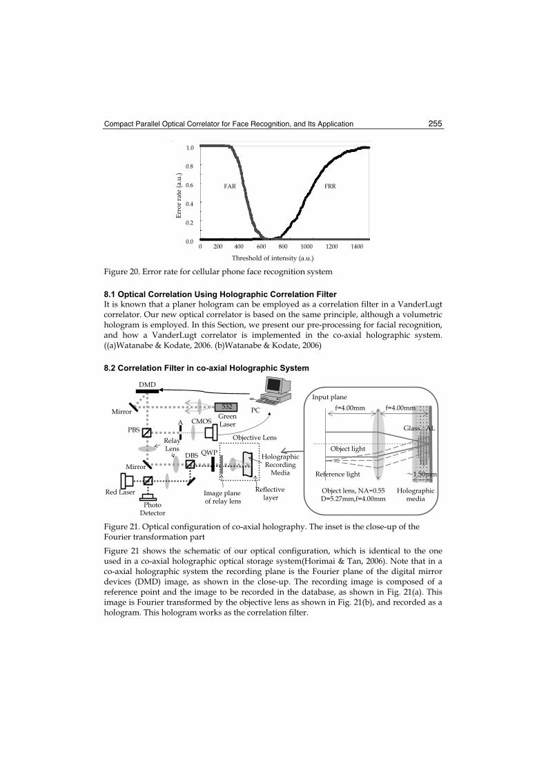
Compact Parallel Optical Correlator for Face Recognition, and Its Application 255
Threshold of intensity (a.u.)
1.0
0.0
Erro
r rat
e (a
.u.)
0.8
0.6
0.4
0.2
0 400 800 1200 14001000600200
FRRFAR
Figure 20. Error rate for cellular phone face recognition system
8.1 Optical Correlation Using Holographic Correlation Filter
It is known that a planer hologram can be employed as a correlation filter in a VanderLugt correlator. Our new optical correlator is based on the same principle, although a volumetric hologram is employed. In this Section, we present our pre-processing for facial recognition, and how a VanderLugt correlator is implemented in the co-axial holographic system. ((a)Watanabe & Kodate, 2006. (b)Watanabe & Kodate, 2006)
8.2 Correlation Filter in co-axial Holographic System
PC
DMD
Green LaserA CMOS
PBS
QWP
Objective Lens
Holographic Recording
Media
Reflectivelayer
532
Red Laser
PhotoDetector
DBSMirror
Relay Lens
Mirror
Image plane of relay lens
Reference light
Object light
f=4.00mm f=4.00mm
Holographicmedia
Object lens, NA=0.55D=5.27mm,f=4.00mm
Glass AL
Input plane
1.50mm
Figure 21. Optical configuration of co-axial holography. The inset is the close-up of the Fourier transformation part
Figure 21 shows the schematic of our optical configuration, which is identical to the one used in a co-axial holographic optical storage system(Horimai & Tan, 2006). Note that in a co-axial holographic system the recording plane is the Fourier plane of the digital mirror devices (DMD) image, as shown in the close-up. The recording image is composed of a reference point and the image to be recorded in the database, as shown in Fig. 21(a). This image is Fourier transformed by the objective lens as shown in Fig. 21(b), and recorded as a hologram. This hologram works as the correlation filter.
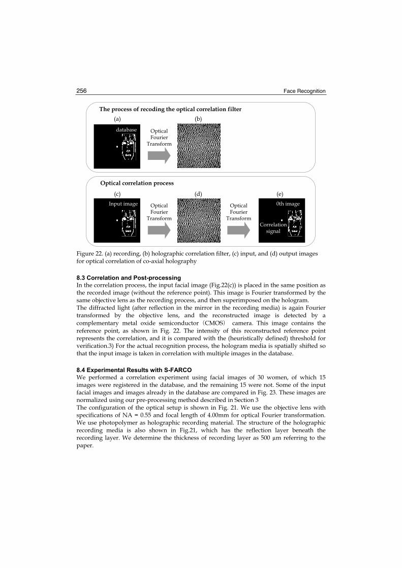
Face Recognition 256
The process of recoding the optical correlation filter
Optical correlation process
database OpticalFourier
Transform
Input image OpticalFourier
Transform
OpticalFourier
Transform
0th image
Correlationsignal
(a) (b)
(c) (d) (e)
Figure 22. (a) recording, (b) holographic correlation filter, (c) input, and (d) output images for optical correlation of co-axial holography
8.3 Correlation and Post-processing
In the correlation process, the input facial image (Fig.22(c)) is placed in the same position as the recorded image (without the reference point). This image is Fourier transformed by the same objective lens as the recording process, and then superimposed on the hologram. The diffracted light (after reflection in the mirror in the recording media) is again Fourier transformed by the objective lens, and the reconstructed image is detected by a complementary metal oxide semiconductor CMOS camera. This image contains the reference point, as shown in Fig. 22. The intensity of this reconstructed reference point represents the correlation, and it is compared with the (heuristically defined) threshold for verification.3) For the actual recognition process, the hologram media is spatially shifted so that the input image is taken in correlation with multiple images in the database.
8.4 Experimental Results with S-FARCO
We performed a correlation experiment using facial images of 30 women, of which 15 images were registered in the database, and the remaining 15 were not. Some of the input facial images and images already in the database are compared in Fig. 23. These images are normalized using our pre-processing method described in Section 3 The configuration of the optical setup is shown in Fig. 21. We use the objective lens with specifications of NA = 0.55 and focal length of 4.00mm for optical Fourier transformation. We use photopolymer as holographic recording material. The structure of the holographic recording media is also shown in Fig.21, which has the reflection layer beneath the recording layer. We determine the thickness of recording layer as 500 μm referring to the paper.
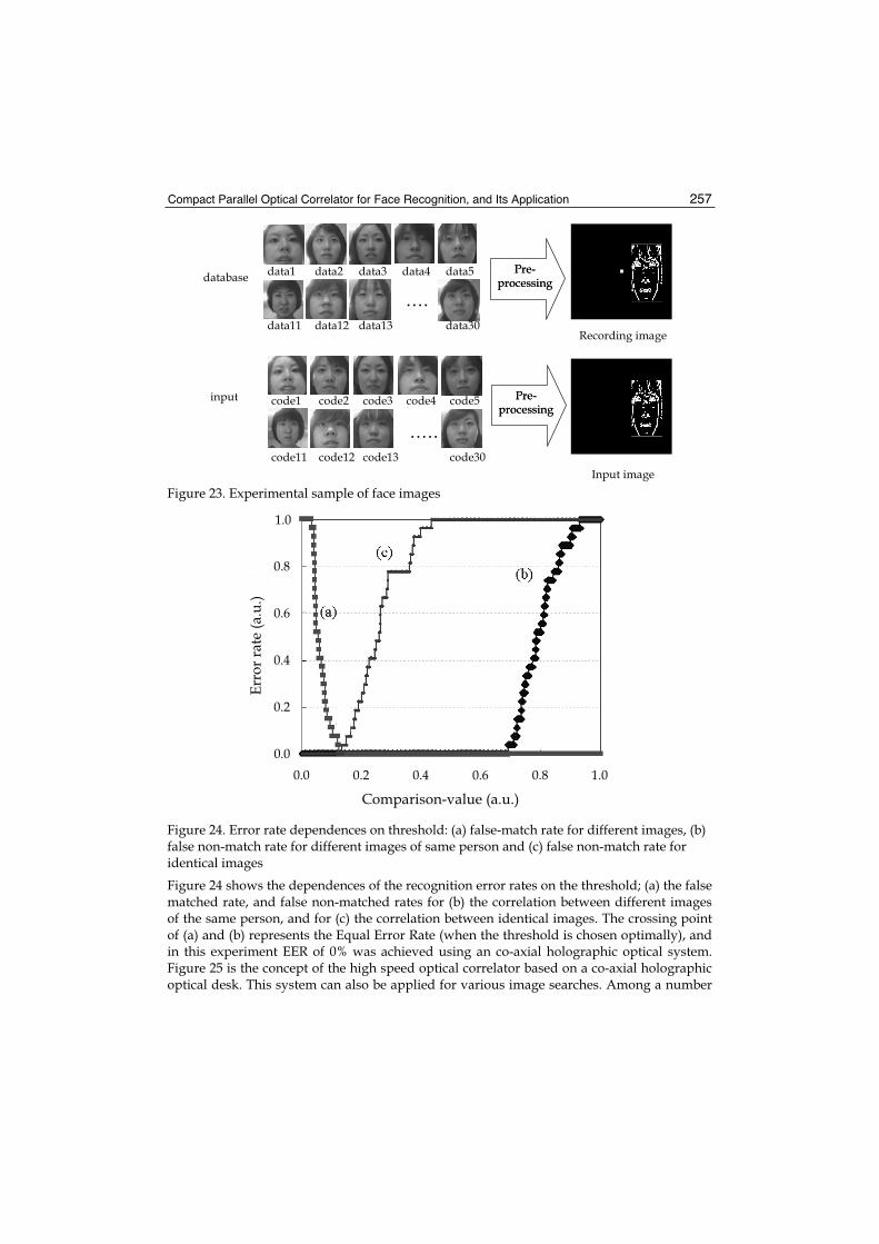
Compact Parallel Optical Correlator for Face Recognition, and Its Application 257
data1 data2 data3 data4 data5
data11 data12 data13 data30Recording image
databasePre-
processingPre-
processing
input
Input image
code1 code2 code3 code4 code5
code11 code12 code13 code30
Pre-processing
Pre-processing
Figure 23. Experimental sample of face images
Comparison-value (a.u.)
Erro
r rat
e (a
.u.)
0.0 1.00.80.60.40.2
0.8
0.6
0.4
0.2
0.0
1.0
Comparison-value (a.u.)
Erro
r rat
e (a
.u.)
0.0 1.00.80.60.40.2
0.8
0.6
0.4
0.2
0.0
1.0
Figure 24. Error rate dependences on threshold: (a) false-match rate for different images, (b) false non-match rate for different images of same person and (c) false non-match rate for identical images
Figure 24 shows the dependences of the recognition error rates on the threshold; (a) the false matched rate, and false non-matched rates for (b) the correlation between different images of the same person, and for (c) the correlation between identical images. The crossing point of (a) and (b) represents the Equal Error Rate (when the threshold is chosen optimally), and in this experiment EER of 0% was achieved using an co-axial holographic optical system. Figure 25 is the concept of the high speed optical correlator based on a co-axial holographic optical desk. This system can also be applied for various image searches. Among a number

Face Recognition 258
of large data storages, only the holographic storage can function not only as memory but also as calculator for e.g. inner product or correlation. We believe that our experimental results contribute to add the value and to broaden the application of holographic storage system. A practical image search system and the analysis of volumetric holographic storage as optical correlator will be reported in another paper. We expect optical correlation of 10 μs/frame, assuming 12,000 pages of hologram in one track rotating at 600 rpm. This means that it is possible to take correlation of more than 100,000 faces/s when applied to face recognition for example.(Fig.25)
High correlation signal at matched address.
Outputplane
DMD
Holographic optical disc
PBS
Image data is stored by matched filter
pattern.
Input data
Code#001
Database
Figure 25. Concept of optical correlator based on optical disc
Cellular phoneCellular phone
SchoolSchool
OfficeOffice
CameraHospital
CameraCameraHospital
Security camera
S-FARCOHomeHome
vast amountsof data
Facerecognition
S-FARCO
Figure 26. Outline of the ultra-fast face recognition server system

Compact Parallel Optical Correlator for Face Recognition, and Its Application 259
9. Future Works
We have proposed a network-style recognition server system based on FARCO. Excellent experimental results, shown in Section 9, proved a wide range of possible applications such as a server into Web and CCTV cameras for public safety. (Fig.26) With its high speed and compactness, these appliances can be used at hospital, school and in the office. Therefore, it has great potential for general use. As one recent example, online search engines such as Google can be counted as a possible venues for exploring potential. At the moment, these types of search engines operate only by keywords. Instead, we are proposing an application of our system to image-search, utilizing its small processing time. Under this image-to-image search, output images with high rate of correlation to the input image will be sieved out and sorted in order. At present, it is very difficult to establish such a system, due to the extremely high volume of the database loaded with images. However, to overcome these obstacles, we are developing a super high-speed and precision image search system using our proposed novel all-optical correlation methods as shown in this chapter.
10. Conclusions
This chapter provides an overview of the basic concept of optical correlation and then explains the significance of the phase information of images. Performance improved greatly by emphasizing the range of wave length on the Fourier plane. Optimizing the algorithms for the face recognition system based on optical correlation, our fast and highly-precise face recognition system, FARCO, was introduced. As an application, a cellular phone-based face recognition system was presented. It is used as an attendance management system for e-learning students at university. False match and false non-match rates are both remarkably low, less than 1 %. In addition, a holographic optical database was applied for a further reduction in processing time. The S-FARCO system was introduced and some prospects for its application were shown. In the future, all-optical correlation, as an ideal type of correlation optical computing, will be more closely examined and experimented on, not only for improving our face recognition system but also for developing image search and installing the system into robots for wider use.
11. Acknowledgements
The authors would like to express their heartfelt thanks to Mr. H. Koizumi of the Topcon Corporation for his collaboration in fabricating the FARCO. The FARCO project was also supported by a Grant-in-Aid for Scientific Research from the Japan Science and Technology Agency and by the Japan Science Technology Corporation (JST). We are indebted to Mr. H. Horimai of the OPTWARE Corporation for the development of the super high speed FARCO, this work being partly supported by a Grant for Practical Application of University R&D Results under the Matching Fund Method (R&D) of the New Energy and Industrial Technology Development Organization (NEDO) We would like to thank Ms. A. Kato, Ms. N. Arima, Ms. M. Ishikawa, Ms. M. Ohta, and all the research staff at Kodate Laboratory at the Faculty of Science, Japan Women’s University. In addition, this chapter refers to a number of articles based on research conducted by graduates of our laboratory.

Face Recognition 260
12. References
kodate, K. Hashimoto, A. & Thapliya, R. (1999). Binary Zone-Plate Array for a Parallel Joint Transform Correlator Applied to Face Recognition. Appl. Opt., Vol.38, No.14, (1999) pp. 2060-3067.
(a)Watanabe, E. & kodate, K. (2005). Implementation of a high-speed face recognition system that uses an optical parallel correlator. Appl. Opt., Vol.44, No.4, (2005) pp. 666-676.
kodate, K. Inaba, R. & Watanabe, E. (2002). Facial recognitiom by a compact parallel optical correlator. Meas. Sci.Technol., Vol.13, (2002.8) pp. 1756-1766.
(b)Watanabe, E. & kodate, K. (2005).Fast Face-Recognition Optical Parallel Correlator Using High Accuracy Correlation Filter. Opt.Rev., Vol.12, No.6, (2005.8) pp. 460-466.
Horner, J, L. & Gianino, D, P. (1984). Phase-only matched filtering. Appl. Opt., Vol.23, No.6, (1982) pp. 812-821.
Bartelt, O, H. (1985). Applications of the tandem component: an element with optimum light efficiency. Appl. Opt., Vol.24, No.22, (1985) pp. 3811.
Watanabe, E. & kodate, K. (2003). Multi-light source compact optical parallel correlator (MLCOPaC) for facial recognition using VCSEL array, Proceedings of SPIE 4829, pp. 208-209, chiba,(2003.11) .
Horimai, H. & Tan, X. (2006). Collinear technology for a holographic versatile disk. Appl. Opt., Vol.45, No.5, (2006) pp. 910-914.
Goodman, J. & Moeller, M. (2004). Introduction to Fourier Optics, Roberts & Company Publishers, 237-238, E, Colo, 0-07-114257-6, USA.
Hecht, E. (1998). Optics, Addison Wesley Longman Inc, 537-545, 0-201-30425-2, USA. Inaba, R. kodate, K. & Watanabe, E. (2003). Security applications of optical face recognition
system: Access control in e-learning. Opt.Rev., Vol.10, No.4, (2003) pp. 255-261. Watanabe, E. & kodate, K. et al.(2006). Highly-accurate face recognition using a novel
filtering correlation, Proceedings of 5th International Conference on Optics-photonics Design & Fabrication, pp.305-306, (2006.12) .
Orihara, Y. Klaus, W. & Kodate, K. et al.(2001). Optimization and Application of Hybrid-Level Binary Zone Plates. Appl. Opt., Vol.40, No.32, (2001) pp. 5877-5885.
(a)Watanabe, E. & kodate, K. et al.(2005). Constructing a safety and security system by medical applications of a fast face recognition optical parallel correlator, Proceedings of SPIE 6027, 60270H, (2005.8) Yunlong Sheng, Songlin Zhuang, Yimo Zhang.
(b)Watanabe, E. & kodate, K. et al.(2005). Constructing a three-dimensional face model by a stereo method and its application to optical parallel face recognition, Proceedings of SPIE 6027, 60270G, (2005.8) Yunlong Sheng, Songlin Zhuang, Yimo Zhang.
(a)Watanabe, E. & kodate, K. (2006).Optical Correlator for Face Recognition Using Collinear Holographic System. J.J.of App.Phy., Vol.45, No.8B, (2005.8) pp. 6759-6761.
(b)Watanabe, E. & kodate, K. (2006). High speed image search engine using collinear holography, Proceedings of SPIE 6245, pp. 147-154, orland,(2006.4) .

13
Human Detection and Gesture Recognition Based on Ambient Intelligence
Naoyuki Kubota Tokyo Metropolitan University
Japan
1. Introduction
Recently, various types of human-friendly robots such as pet robots, amusement robots, and partner robots, have been developed for the next generation society. The human-friendly robots should perform human recognition, voice recognition, and gesture recognition in order to realize natural communication with a human. Furthermore, the robots should coexist in the human environments based on learning and adaptation. However, it is very difficult for the robot to successfully realize these capabilities and functions under real world conditions. Two different approaches have been discussed to improve these capabilities and functions of the robots. One approach is to use conventional intelligent technologies based on various sensors equipped on a robot. As a result, the size of a robot becomes large. The other approach is to use ambient intelligence technologies of environmental systems based on the structured information available to a robot. The robot directly receives the environmental information through a local area network without measurement by the robot itself. In the following, we explain the current status of researches on sensor networks and interactive behavior acquisition from the viewpoint of ambient intelligence.
1.1 Ambient Intelligence
For the development of sensor network and ubiquitous computing, we should discuss the intelligence technologies in the whole system of robots and environmental systems. Here intelligence technologies related with measurement, transmission, modeling, and control of environmental information is called ambient intelligence. The concept of ambient intelligence was discussed by Hagras et.al. (Doctor et al., 2005). Their main aim is to improve the qualities of life based on computational artifacts, but we focus on the technologies for the co-existence of humans and robots in the same space. From the sensing point of view, a robot is considered as a movable sensing device, and an environmental system is considered as a fixed sensing device. If the environmental information is available from the environmental system, the flexible and dynamic perception can be realized by integrating environmental information. The research on wireless sensor networks combines three components of sensing, processing, and communicating into a single tiny device (Khemapech et al., 2005). The main roles of sensor networks are (1) environmental data gathering, (2) security monitoring, (3)

Face Recognition 262
and object tracking. In the environmental data gathering, the data measured at each node are periodically transmitted to a database server. While the synchronization of the measurement is very important to improve the accuracy of data in the environmental data gathering, an immediate and reliable emergency alert system is very important in the security monitoring. Furthermore, a security monitoring system does not need to transmit data to an emergency alert system, but the information on features or situations should be transmitted as fast as possible. Therefore, the basic network architecture is different between data gathering and security monitoring. On the other hand, the object tracking is performed through a region monitored by a sensor network. Basically, objects can be tracked by tagging them with a small sensor node. Radio frequency identification (RFID) tags are often used for the tracking system owing to low cost and small size. Sensor networks and ubiquitous computing have been incorporated into robotics. These researches are called network robotics and ubiquitous robotics, respectively (Kim et al., 2004). The ubiquitous computing integrates computation into the environment (Satoh, 2006). The ubiquitous computing is conceptually different from sensor networks, but both aim at the same research direction. If the robot can receive the environmental data through the network without the measurement by sensors, the size of the robot can be easily reduced and the received environmental data are more precise because the sensors equipped in the environment is designed suitable to the environmental conditions. On the other hand, network robots are divided into three types; visible robots, unconscious robots, and virtual robots (Kemmotsu, 2005). The role of visible robots is to act on users with their physical body. The role of unconscious robots is mainly to gather environmental data, and this kind of unconscious robot is invisible to users. A virtual robot indicates a software or agent in a cyber world. A visible robot can easily perceive objects by receiving object information from RFID tags, and this technology has been applied for the robot navigation and the localization of the self-position (Kulyukin et al., 2004). Hagras et al. developed iDorm as a multi-function space (Doctor et al., 2005). Furthermore, Hashimoto et al. proposed Intelligent Space (iSpace) in order to achieve human-centered services, and developed distributed intelligent network devices composed of color CCD camera including processing and networking units (Morioka & Hashimoto, 2004). A robot can be used not only as a human-friendly life-support system (Mori et al., 2005), but also as an interface connecting the physical world with the cyber world.
1.2 Interactive Behavioral Acquisition
In general, the behavioral acquisition used in robotics can be classified into supervised learning and self-learning (Figure1). The self-learning is defined as unsupervised learning performed by trial-and-error without exact target teaching signals for motion reproduction. Supervised learning in behavior acquisition is divided into social learning and error-based learning. For example, least mean square algorithms are applied for behavioral learning when exact target teaching signals are given to a robot. On the other hand, the observed data, instead of exact target teaching signals, are used in social leaning. The social learning is performed between two or more agents. Basically, social learning is divided into imitative learning, instructive learning, and collaborative learning (Morikawa et al., 2001). Imitation (Billard, 2002) is a powerful tool for gestural interaction among children and for teaching how to behave to children by parents. Furthermore, the imitation is often used for communication among children, and the gestures are useful to understand the intentions
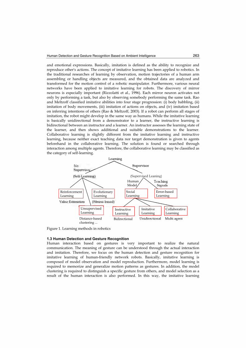
Human Detection and Gesture Recognition Based on Ambient Intelligence 263
and emotional expressions. Basically, imitation is defined as the ability to recognize and reproduce other's actions. The concept of imitative learning has been applied to robotics. In the traditional researches of learning by observation, motion trajectories of a human arm assembling or handling objects are measured, and the obtained data are analyzed and transformed for the motion control of a robotic manipulator. Furthermore, various neural networks have been applied to imitative learning for robots. The discovery of mirror neurons is especially important (Rizzolatti et al., 1996). Each mirror neuron activates not only by performing a task, but also by observing somebody performing the same task. Rao and Meltzoff classified imitative abilities into four stage progression: (i) body babbling, (ii) imitation of body movements, (iii) imitation of actions on objects, and (iv) imitation based on inferring intentions of others (Rao & Meltzoff, 2003). If a robot can perform all stages of imitation, the robot might develop in the same way as humans. While the imitative learning is basically unidirectional from a demonstrator to a learner, the instructive learning is bidirectional between an instructor and a learner. An instructor assesses the learning state of the learner, and then shows additional and suitable demonstrations to the learner. Collaborative learning is slightly different from the imitative learning and instructive learning, because neither exact teaching data nor target demonstration is given to agents beforehand in the collaborative learning. The solution is found or searched through interaction among multiple agents. Therefore, the collaborative learning may be classified as the category of self-learning.
ImitativeLearning
InstructiveLearning
ReinforcementLearning
EvolutionaryLearning
HumanModel
Error-basedLearning
Social Learning
(Supervised Leaning)
UnsupervisedLearning
BidirectionalDistance-basedclustering ...
CollaborativeLearning
Figure 1. Learning methods in robotics
1.3 Human Detection and Gesture Recognition
Human interaction based on gestures is very important to realize the natural communication. The meaning of gesture can be understood through the actual interaction and imitation. Therefore, we focus on the human detection and gesture recognition for imitative learning of human-friendly network robots. Basically, imitative learning is composed of model observation and model reproduction. Furthermore, model learning is required to memorize and generalize motion patterns as gestures. In addition, the model clustering is required to distinguish a specific gesture from others, and model selection as a result of the human interaction is also performed. In this way, the imitative learning

Face Recognition 264
requires various learning capabilities of model observation, model clustering, model selection, model reproduction, and model learning simultaneously. First of all, the robot detects a human based on image processing with a steady-state genetic algorithm (SSGA) (Syswerda, 1991). Next, a series of the movements of the human hand by image processing as model observation, or the hand motion pattern, is extracted by a spiking neural network (Gerstner, 1999). Furthermore, SSGA is used for generating a trajectory similar to the human hand motion pattern as model reproduction (Kubota, Nojima et al., 2006). In the following, we explain the methods for the human detection and gesture recognition based on ambient intelligence.
2. Partner Robots and Environmental System
We developed two different types of partner robots; a human-like robot called Hubot (Kubota, Nojima et al., 2006) and a mobile PC called MOBiMac (Kubota, Tomioka et al., 2006) in order to realize the social communication with humans. Hubot is composed of a mobile base, a body, two arms with grippers, and a head with pan-tilt structure. The robot has various sensors such as a color CCD camera, two infrared line sensors, a microphone, ultrasonic sensors, and touch sensors (Figure 2(a)). The color CCD camera can capture an image with the range of -30˚ and 30˚ in front of the robot. Two CPUs are used for sensing, motion control, and wireless network communication. The robot can take various behaviors like a human. MOBiMac is also composed of two CPUs used for PC and robotic behaviors (Figure 2(b)). The robot has two servo motors, four ultrasonic sensors, four light sensors, a microphone, and a CCD camera. The basic behaviors of these robots are visual tracking, map building, imitative learning (Kubota, 2005), human classification, gesture recognition, and voice recognition. These robots are networked, and share environmental data among each other. Furthermore, the environmental system based on a sensor network provides a robot with its environmental data measured by the equipped sensors. Human detection is one of the most important functions in the ambient intelligence space. The visual angle of the robot is very limited, while the environmental system is designed to observe the wide range of the environment. Therefore, human detection can be easily performed by the monitoring of the environmental system or by the cooperative search of several robots based on the ambient intelligence (Figure 3). In the following sections, we explain how to detect a human based on image processing.
(a) Hubot (b) MOBiMac
Figure 2. Hardware architecture of partner robots
sensors
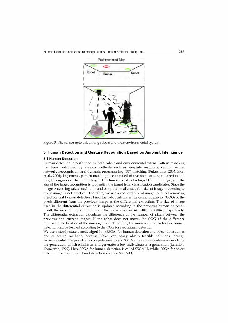
Human Detection and Gesture Recognition Based on Ambient Intelligence 265
Figure 3. The sensor network among robots and their environmental system
3. Human Detection and Gesture Recognition Based on Ambient Intelligence
3.1 Human Detection
Human detection is performed by both robots and envrionmental sytem. Pattern matching has been performed by various methods such as template matching, cellular neural network, neocognitron, and dynamic programming (DP) matching (Fukushima, 2003; Mori et al., 2006). In general, pattern matching is composed of two steps of target detection and target recognition. The aim of target detection is to extract a target from an image, and the aim of the target recognition is to identify the target from classification candidates. Since the image processing takes much time and computational cost, a full size of image processing to every image is not practical. Therefore, we use a reduced size of image to detect a moving object for fast human detection. First, the robot calculates the center of gravity (COG) of the pixels different from the previous image as the differential extraction. The size of image used in the differential extraction is updated according to the previous human detection result; the maximum and minimum of the image sizes are 640×480 and 80×60, respectively. The differential extraction calculates the difference of the number of pixels between the previous and current images. If the robot does not move, the COG of the difference represents the location of the moving object. Therefore, the main search area for fast human detection can be formed according to the COG for fast human detection. We use a steady-state genetic algorithm (SSGA) for human detection and object detection as one of search methods, because SSGA can easily obtain feasible solutions through environmental changes at low computational costs. SSGA simulates a continuous model of the generation, which eliminates and generates a few individuals in a generation (iteration) (Syswerda, 1999). Here SSGA for human detection is called SSGA-H, while SSGA for object detection used as human hand detection is called SSGA-O.

Face Recognition 266
Human skin and hair colors are extracted by SSGA-H based on template matching. Figure 4 shows a candidate solution of a template used for detecting a target. A template is composed of numerical parameters of gi,1H, gi,2H, gi,3H, and gi,4H. The number of individuals is G. One iteration is composed of selection, crossover, and mutation. The worst candidate solution is eliminated ("Delete least fitness" selection), and is replaced by the candidate solution generated by the crossover and the mutation. We use elitist crossover and adaptive mutation. The elitist crossover randomly selects one individual and generates an individual by combining genetic information from the randomly selected individual and the best individual. Next, the following adaptive mutation is performed to the generated individual,
gi , jH ← gi , j
H + α jH ⋅
fmaxH − fi
H
fmaxH − fmin
H+ β j
H ⋅N 0,1( ) (1)
where fiH is the fitness value of the ith individual, fmaxH and fminH are the maximum and minimum of fitness values in the population; N(0,1) indicates a normal random variable with a mean of zero and a variance of one; jH and jH are the coefficient (0< jH<1.0) and offset ( jH>0), respectively. In the adaptive mutation, the variance of the normal random number is relatively changed according to the fitness values of the population. Fitness value is calculated by the following equation,
fiH = CSkin
H + CHairH +η1
H ⋅CSkinH ⋅CHair
H −η2H ⋅COther
H (2)
where CSkinH, CHairH and COtherH indicate the numbers of pixels of the colors corresponding to human skin, human hair, and other colors, respectively; 1H and 2H are the coefficients ( 1H, 2H>0). Therefore, this problem results in the maximization problem. The iteration of SSGA-H is repeated until the termination condition is satisfied.
Figure 4. A template used for human detection in SSGA-H
3.2 Human Hand Detection
We proposed a method for human hand detection based on the finger color and edges (Kubota & Abe, 2006), but we assume the human uses objects such as balls and blocks for performing a gesture interacting with a robot. Because the main focus is the gesture recognition based on human hand motion and the exact human hand detection is out of scope in this chapter. Therefore, we focus on color-based object detection with SSGA-O based on template matching. The shape of a candidate template is generated by the SSGA-O. We assume the human uses objects such as balls and blocks for performing a gesture interacting with a robot. Figure 5 shows a candidate template used for detecting a target where the jth point gi,jO of the ith template is represented by (gi,1O+gi,jOcos(gi,j+1O),

Human Detection and Gesture Recognition Based on Ambient Intelligence 267
gi,2O+gi,jOsin(gi,j+1O)), i=1, 2, ... , n, j=3, ... , 2�m+2; Oi (=(gi,1O, gi,2O)) is the center of a candidate template on the image; n and m are the number of candidate templates and the searching points used in a template, respectively. Therefore, a candidate template is composed of numerical parameters of (gi,1O, gi,2O,... , gi,2m+2O). We used an octagonal template (m=8). The fitness value of the ith candidate template is calculated as follows.
fiO = CT arg et
O −ηO ⋅COtherO (3)
where O is the coefficient for penalty ( O>0); CTargetO and COtherO indicate the numbers of pixels of a target and other colors included in the template, respectively. The target color is selected according to the pixel color occupied mostly in the template candidate. Therefore, this problem also results in the maximization problem. The robot extracts human hand motion from the series of images by using SSGA-O where the maximal number of images is TG. The sequence of the hand positions is represented by G(t)=(Gx(t), Gy(t)) where t=1, 2, ... , TG.
Figure 5. A template used for object detection in SSGA-O
3.3 Human Hand Motion Extraction
Various types of artificial neural networks have been proposed to realize clustering, classification, nonlinear mapping, and control (Jang et al., 1997; Kuniyoshi & Shimozaki, 2003; Rumelhart et al., 1986). Basically, artificial neural networks are classified into pulse-coded neural networks and rate-coded neural networks from the viewpoint of abstraction level (Gerstner, 1999). A pulse-coded neural network approximates the dynamics with the ignition phenomenon of a neuron, and the propagation mechanism of the pulse between neurons. Hodgkin-Huxley model is one of the classic neuronal spiking models with four differential equations. An integrate-and-fire model with a first-order linear differential equation is known as a neuron model of a higher abstraction level. A spike response model is slightly more general than the integrate-and-fire model, because the spike response model can choose kernels arbitrarily. On the other hand, rate-coded neural networks neglect the pulse structure, and therefore are considered as neuronal models of the higher level of abstraction. McCulloch-Pitts and Perceptron are well known as famous rate coding models (Anderson & Rosenfeld, 1988). One important feature of pulse-coded neural networks is the capability of temporal coding. In fact, various types of spiking neural networks (SNNs) have been applied for memorizing spatial and temporal contexts. Therefore, we apply a SNN for memorizing several motion patterns of a human hand, because the human hand motion has specific dynamics. We use a simple spike response model to reduce the computational cost. First of all, the internal state hi(t) is calculated as follows;

Face Recognition 268
hi(t) = tanh hisyn(t)+ hi
ext (t)+ hiref (t)( ) (4)
Here hyperbolic tangent is used to avoid the bursting of neuronal fires, hiext(t) is the input to the ith neuron from the external environment, and hisyn(t) including the output pulses from other neurons is calculated by,
hisyn(t) = γ syn ⋅hi(t − 1)+ wj ,i ⋅hj
EPSP (t)j=1, j≠i
N
(5)
Furthermore, hiref(t) indicates the refractoriness factor of the neuron; wj,i is a weight coefficient from the jth to ith neuron; hjEPSP(t) is the excitatory postsynaptic potential (EPSP) of the jth neuron at the discrete time t; N is the number of neurons; syn is a temporal discount rate. The presynaptic spike output is transmitted to the connected neuron according to EPSP. The EPSP is calculated as follows;
hiEPSP(t) = κ npi(t − n)
n=0
T
(6)
where is the discount rate (0<k<1.0); pi(t) is the output of the ith neuron at the discrete time t; T is the time sequence to be considered. If the neuron is fired, R is subtracted from the refractoriness value in the following,
hiref (t) =
γ ref ⋅hiref (t − 1)− R if pi(t − 1) = 1
γ ref ⋅hiref (t − 1) otherwise
(7)
where ref is a discount rate. When the internal potential of the ith neuron is larger than the predefined threshold, a pulse is outputted as follows;
pi(t) =1 if hi
ref (t) ≥ qi
0 otherwise (8)
where qi is a threshold for firing. Here spiking neurons are arranged on a planar grid (Figure 6) and N=25. By using the value of a human hand position, the input to the ith neuron is calculated by the Gaussian membership function as follows;
hiext (t) = exp −
ci − G(t)2
2σ 2 (9)
where ci=(cx,i, cy,i) is the position of the ith spiking neuron on the image; � is a standard deviation. The sequence of pulse outputs pi(t) is obtained by using the human hand positions G(t). The weight parameters are trained based on the temporal Hebbian learning rule as follows,
wj ,i ← tanh γ wgt ⋅wj ,i +ξwgt ⋅hjEPSP (t − 1)⋅hi
EPSP (t)( ) (10)
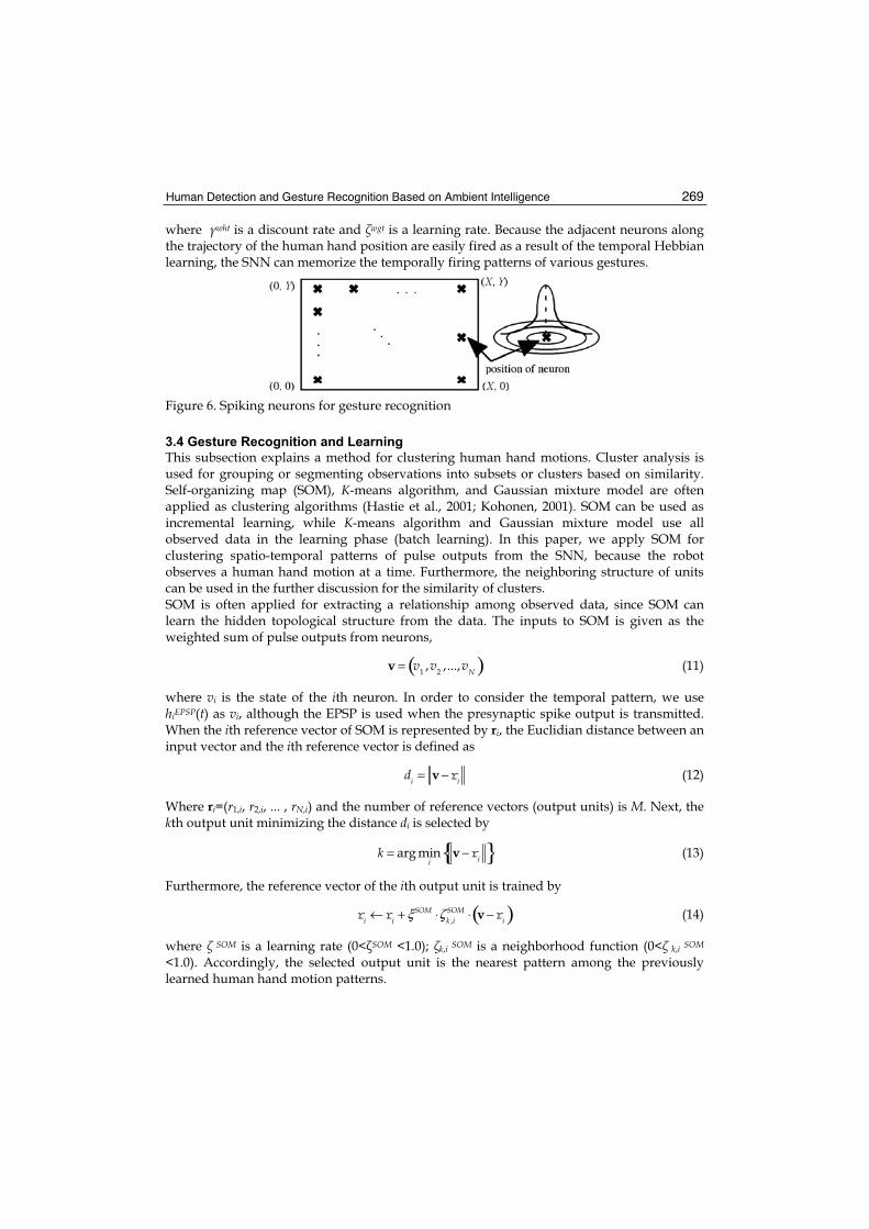
Human Detection and Gesture Recognition Based on Ambient Intelligence 269
where wht is a discount rate and wgt is a learning rate. Because the adjacent neurons along the trajectory of the human hand position are easily fired as a result of the temporal Hebbian learning, the SNN can memorize the temporally firing patterns of various gestures.
Figure 6. Spiking neurons for gesture recognition
3.4 Gesture Recognition and Learning
This subsection explains a method for clustering human hand motions. Cluster analysis is used for grouping or segmenting observations into subsets or clusters based on similarity. Self-organizing map (SOM), K-means algorithm, and Gaussian mixture model are often applied as clustering algorithms (Hastie et al., 2001; Kohonen, 2001). SOM can be used as incremental learning, while K-means algorithm and Gaussian mixture model use all observed data in the learning phase (batch learning). In this paper, we apply SOM for clustering spatio-temporal patterns of pulse outputs from the SNN, because the robot observes a human hand motion at a time. Furthermore, the neighboring structure of units can be used in the further discussion for the similarity of clusters. SOM is often applied for extracting a relationship among observed data, since SOM can learn the hidden topological structure from the data. The inputs to SOM is given as the weighted sum of pulse outputs from neurons,
v = v1 ,v2 ,...,vN( ) (11)
where vi is the state of the ith neuron. In order to consider the temporal pattern, we use hiEPSP(t) as vi, although the EPSP is used when the presynaptic spike output is transmitted. When the ith reference vector of SOM is represented by ri, the Euclidian distance between an input vector and the ith reference vector is defined as
di = v−ri (12)
Where ri=(r1,i, r2,i, ... , rN,i) and the number of reference vectors (output units) is M. Next, the kth output unit minimizing the distance di is selected by
k = arg mini
v−ri{ } (13)
Furthermore, the reference vector of the ith output unit is trained by
ri ←ri +ξSOM ⋅ζ k ,iSOM ⋅ v−ri( ) (14)
where SOM is a learning rate (0< SOM <1.0); k,i SOM is a neighborhood function (0< k,i SOM
<1.0). Accordingly, the selected output unit is the nearest pattern among the previously learned human hand motion patterns.

Face Recognition 270
4. Experiments
This section shows several experimental results of human detection and gesture recognition. We conducted several experiments of human detection by the environmental system and the robot (Kubota & Nishida, 2006; Sasaki & Kubota, 2006). Figures 7 and 8 show human detection results by SSGA-H from the ceiling view and from the robot view, respectively. The environmental system detects two people in the complicated background in Figure 7. In Figure 8 (a), first the robot used the high resolution of images to detect a walking human. Afterward, as the human gradually came toward the front of the robot, the robot used the lower resolution of images to reduce computational cost and detected the human (Figure 8 (b)).
Figure 7. Human detection results from the ceiling camera of the environmental system by SSGA-H
Figure 8. Human detection results from the robot by SSGA-H
We conducted several experiments of gesture recognition. The number of units used in SOM is 8. Figures 9 and 10 show examples of human hand motion and the learning of SNN, respectively. The human moves his hand from the upper left to the lower right through upper right on the human position. The EPSP based on spike outputs does not cover the human hand motion at the first trial (Figure 10 (a)), but after learning, the EPSP successfully covers the human hand motion based on the trained weight connections where the depth of color indicates the strength of weight connections between two neurons (Figure 10 (b)).
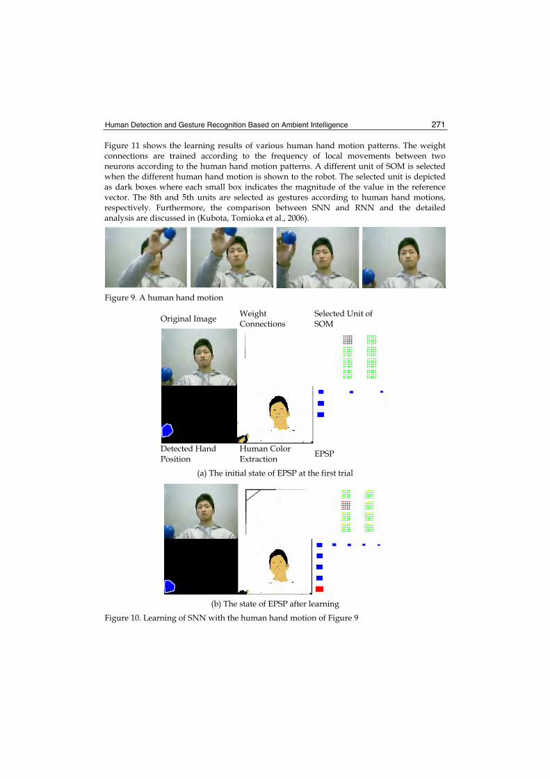
Human Detection and Gesture Recognition Based on Ambient Intelligence 271
Figure 11 shows the learning results of various human hand motion patterns. The weight connections are trained according to the frequency of local movements between two neurons according to the human hand motion patterns. A different unit of SOM is selected when the different human hand motion is shown to the robot. The selected unit is depicted as dark boxes where each small box indicates the magnitude of the value in the reference vector. The 8th and 5th units are selected as gestures according to human hand motions, respectively. Furthermore, the comparison between SNN and RNN and the detailed analysis are discussed in (Kubota, Tomioka et al., 2006).
Figure 9. A human hand motion
Original Image WeightConnections
Selected Unit of SOM
Detected Hand Position
Human Color Extraction EPSP
(a) The initial state of EPSP at the first trial
(b) The state of EPSP after learning
Figure 10. Learning of SNN with the human hand motion of Figure 9

Face Recognition 272
(a) A recognition result of human hand motion of the 8 figure; the 8th unit is selected.
A recognition result of the human hand motion from the left to right; the 5th unit is selected.
Figure 11. Gesture recognition by SNN and SOM after learning
5. Summary
This chapter introduced the methods for human detection and gesture recognition based on ambient intelligence. The experimental results show the effectiveness of the methods for human detection and gesture recognition, but we should use various types of sensory information in addition to visual images. We proposed the concept of evolutionary robot vision. The main sensory information is vision, but we can integrate and synthesize various types of sensory information for image processing. Possible sensory information to improve the performance is distance. We developed a 3D modeling method based on CCD cameras and a laser range finder with a small and compact pan-tilt mechanism. We intend to develop a gesture recognition method based on various types of sensory information. Furthermore, network robots based on ambient intelligece are an attractive approach to realize sophisticated services in the next generation society. One of attractive approaches is the SICE City project. The aim of SICE city project is to build up the methodology and concept in the city design to realize sophisticated services for residents based on measurement technology, network technology, control technology, and systems theory. We will discuss the applicability of human detection, human recognition, gesture recognition, and motion recognition based on ambient intelligence to human-friendly functions in the city design.

Human Detection and Gesture Recognition Based on Ambient Intelligence 273
6. Acknowledgment
The author would like to thank K.Nishida, T. Shimizu, and Y. Tomioka for all their help. This research is partially supported by grants-in-aid for scientific research on priority areas (B) 17700204 from Japan Society for the Promotion of Science.
7. References
Anderson, J. A. & Rosenfeld, E. (1988). Neurocomputing, The MIT Press, Cambridge, Massachusetts, US
Billard, A. (2002). Imitation, Handbook of Brain Theory and Neural Networks, Arbib, M. A., (Ed.), 566-569, MIT Press, Cambridge, Massachusetts, US
Doctor, F.; Hagras, H. & Callaghan, V. (2005). A type-2 fuzzy embedded agent to realise ambient intelligence in ubiquitous computing environments, Information Sciences,Vol.171, Issue 4, pp.309-334
Fukushima, K. (2003). Neural network model restoring partly occluded patterns, Knowledge-Based Intelligent Information and Engineering Systems, (7th International Conference, KES 2003), Part II, eds: V. Palade, R. J. Howlett, L. Jain, Berlin - Heidelberg: Springer-Verlag, pp. 131-138
Gerstner, W. (1999). Spiking neurons, Pulsed Neural Networks, Maass, W. & Bishop, C.M., (Ed.), 3-53, MIT Press, Cambridge, Massachusetts, US
Hastie, T.; Tibshirani, R. & Friedman, J. (2001). The Elements of Statistical Learning: Data Mining, Inference, and Prediction, Springer-Verlag, New York
Jang, J.-S.R.; Sun, C.-T. & Mizutani, E. (1997). Neuro-Fuzzy and Soft Computing, Prentice-Hall Inc.
Kemmotsu, K.; Tomonaka, T.; Shiotani, S.; Koketsu, Y. & Iehara, M. (2005). Recognizing human behaviors with vision sensors in network robot systems, Proceedings of The 1st Japan-Korea Joint Symposium on Network Robot Systems (JK-NRS2005)
Khemapech, I.; Duncan, I. & Miller, A. (2005). A survey of wireless sensor networks technology, Proceedings of The 6th Annual PostGraduate Symposium on The Convergence of Telecommunications, Networking and Broadcasting
Kim, J-H.; Kim, Y-D. & Lee, K-H. (2004). The third generation of robotics: ubiquitous robot, Proceedings of 2nd International Conference on Autonomous Robots and Agents(ICARA 2004), pp.1-12, Palmerston North, New Zealand
Kohonen, T. (2001). Self-Organizing Maps, 3rd Edition, Springer-Verlag, Berlin, Heidelberg Kubota, N. (2005). Computational Intelligence for Structured Learning of A Partner Robot
Based on Imitation, Information Science, No. 171, pp.403-429 Kubota, N. & Abe, M. (2006). Human hand detection for gestures recognition of a partner
robot, Proceedings of World Automation Congress (WAC) 2006, ifmip_214, Budapest, Hungary
Kubota, N. & Nishida, K. (2006). Cooperative perceptual systems for partner robots based on sensor network, International Journal of Computer Science and Network Security (IJCSNS), Vol. 6, No. 11, pp. 19-28, ISSN 1738-7906
Kubota, N.; Nojima, Y.; Kojima, F. & Fukuda, T. (2006). Multiple Fuzzy State-Value Functions for Human Evaluation through Interactive Trajectry Planning of a Partner Robot, Soft Computing, Vol.10, No.10 pp.891-901

Face Recognition 274
Kubota, N.; Tomioka, Y. & Abe, M. (2006). Temporal coding in spiking neural network for gestures recognition of a partner robot, Proceedings of Joint 3rd International Conference on Soft Computing and Intelligent Systems and 7th International Symposium on advanced Intelligent Systems (SCIS & ISIS 2006), pp. 737-742, Tokyo, Japan
Kulyukin, et al., (2004). RFID in robot-assisted indoor navigation for the visually impaired, Proceedings of 2004 IEEE/RSJ International Conference on Intelligent Robots and Systems (IROS 2004), pp. 1979-1984
Kuniyoshi, Y. & Shimozaki, M. (2003). A self-organizing neural model for context-based action recognition, Proceedings of IEEE EMBS Conference on Neural Engineering, pp. 442-445, Capri Island, Italy.
Mori, A.; Uchida, S.; Kurazume, R.; Taniguchi, R.; Hasegawa, T. & Sakoe, H. (2006). Early recognition and prediction of gestures, Proceedings of International Conference on Pattern Recognition, pp. 560-563, Hong Kong, China
Morikawa, K.; Agarwal, S.; Elkan, C. & Cottrell, G. (2001). A taxonomy of computational and social learning, Proceedings of Workshop on Developmental Embodied Cognition
Morioka, K. & Hashimoto, H. (2004). Appearance based object identification for distributed vision sensors in intelligent space, Proceedings of IEEE/RSJ International Conference on Intelligent Robots and Systems (IROS 2004), pp.199-204
Nolfi, S. & Floreano, D. (2000). Evolutionary Robotics: The Biology, Intelligence, and Technology of Self-Organizing Machines, The MIT Press, Cambridge, Massachusetts, US
Rao, R. P. N. & Meltzoff, A. N. (2003). Imitation leaning in infants and robots: towards probabilistic computational models, Proceedings of Artificial Intelligence and Simulation of Behaviors, pp. 4-14
Rumelhart, D. E.; McClelland, J. L. & the PDP Research Group. (1986). Parallel Distributed Processing: Explorations in the Microstructure of Cognition, Volumes 1, The MIT Press, Cambridge, Massachusetts, US
Sasaki, H. & Kubota, N. (2006). Map building and monitoring for environmental information gathering based on intelligent networked robots, Proceedings of Environmental Modelling and Simulation 2006, 556-070, ISBN 0-88986-619-8, St. Thomas, USVI, USA.
Satoh, I. (2006). Location-based services in ubiquitous computing environments, International Journal of Digital Libraries, ISNN 1432-1300
Syswerda, G. (1991) A study of reproduction in generational and steady-state genetic algorithms, Genetic Algorithms, Morgan Kaufmann Publishers Inc., San Mateo
14
Investigating Spontaneous Facial Action Recognition through
AAM Representations of the Face
Simon Lucey, Ahmed Bilal Ashraf and Jeffrey F. Cohn Carnegie Mellon University
USA
1. Introduction
The Facial Action Coding System (FACS) [Ekman et al., 2002] is the leading method for measuring facial movement in behavioral science. FACS has been successfully applied, but not limited to, identifying the differences between simulated and genuine pain, differences betweenwhen people are telling the truth versus lying, and differences between suicidal and non-suicidal patients [Ekman and Rosenberg, 2005]. Successfully recognizing facial actions is recognized as one of the “major” hurdles to overcome, for successful automated expression recognition. How one should represent the face for effective action unit recognition is the main topic of interest in this chapter. This interest is motivated by the plethora of work in existence in other areas of face analysis, such as face recognition [Zhao et al., 2003], that demonstrate the benefit of representation when performing recognition tasks. It is well understood in the field of statistical pattern recognition [Duda et al., 2001] given a fixed classifier and training set that how one represents a pattern can greatly effect recognition performance. The face can be represented in a myriad of ways. Much work in facial action recognition has centered solely on the appearance (i.e., pixel values) of the face given quite a basic alignment (e.g., eyes and nose). In our work we investigate the employment of the Active Appearance Model (AAM) framework [Cootes et al., 2001, Matthews and Baker, 2004] in order to derive effective representations for facial action recognition. Some of the representations we will be employing can be seen in Figure 1. Experiments in this chapter are run across two action unit databases. The Cohn- Kanade FACS-Coded Facial Expression Database [Kanade et al., 2000] is employed to investigate the effect of face representation on posed facial action unit recognition. Posed facial actions are those that have been elicited by asking subjects to deliberately make specific facial actions or expressions. Facial actions are typically recorded under controlled circumstances that include full-face frontal view, good lighting, constrained head movement and selectivity in terms of the type and magnitude of facial actions. Almost all work in automatic facial expression analysis has used posed image data and the Cohn-Kanade database may be the database most widely used [Tian et al., 2005]. The RU-FACS Spontaneous Expression Database is employed to investigate how these same representations affect spontaneous facialaction unit recognition. Spontaneous facial actions are representative of “real-world” facial

Face Recognition 276
actions. They typically occur in less controlled environments, with non-frontal pose, smaller face image size, small to moderate head movement, and less intense and often more complex facial actions. Spontaneous actions units are elicited indirectly from subjects through environmental variables (e.g., showing a subject something associated with happiness which then indirectly results in a smile). Although harder to collect and annotate, spontaneous facial actions are preferable to posed as they are representative of real world facial actions. Most automated facial action recognition systems have only been evaluated on posed facial action data [Donato et al., 1999, Tian et al., 2001] with only a small number of studies being conducted on spontaneous data [Braathen et al., 2001, Bartlett et al., 2005]. This study extends much of the earlier work we conducted in [Lucey et al., 2006]. We greatly expand upon our earlier work in a number of ways. First, we expand the number of AUs analyzed from 4, centered around the brow region, to 15, stemming from all regions of the face. Second, we investigate how representation affects both posed and spontaneous actions units by running our experiments across both kinds of datasets. Third, we report results in terms of verification performance (i.e., accept or reject that a claimed AU observation is that AU) rather than identification performance (i.e., determine out of a watchlist of AU combinations which class does this observation belong to?). The verification paradigm is preferable over identification as it provides a natural mechanism for dealing with simultaneously occurring AUs and is consistent with existing literature [Bartlett et al., 2005].
1.1 Background
One of the first studies into representations of the face, for automatic facial action recognition, was conducted by Donato et al. [1999]. Motivated by the plethora of work previously performed in the face recognition community, this study was restricted to 2-D appearance based representations of the face (e.g. raw pixels, optical flow, Gabor filters, etc.) as well as data-driven approaches for obtaining compact features (e.g. PCA, LDA, ICA, etc.). These appearance based approaches were broadly categorized into holistic, also referred to as monolithic, and parts-based representations. In the ensuing literature, appearance based approaches have continued to be popular as demonstrated by the recent feature evaluation paper by Bartlett et al. [2005]. A major criticism of purely appearance based approaches however, is their lack of shape registration. When “realworld” variation occurs, their lack of shape registration (i.e. knowledge of the position of the eyes, brow, mouth, etc.) makes normalizing for translation and rotation difficult to achieve. Model-based approaches offer an alternative to appearance based approaches for representing the face. Typical approaches have beenActive ShapeModels (ASMs) [Cootes et al., 2001] and Active Appearance Models (AAMs) [Cootes et al., 2001, Matthews and Baker, 2004] in which both appearance and shape can be extracted and decoupled from one another. Model-based approaches to obtaining representations, like those possible with AAMs, have an inherent benefit over purely appearance based representations in the sense they can account and attempt to normalize for many types of “real-world” variation.

Investigating Spontaneous Facial Action Recognition through AAM Representations of the Face 277
(a) (b) (c) Figure 1. This figure depicts the different levels of shape removal from the appearance. Column (a) depicts the initial scenario in which all shape and appearance is preserved. In (b) geometric similarity is removed from both the shape and appearance; and in (c) shape (including similarity) has been removed leaving the average face shape and what we refer to as the face image’s canonical appearance. Features derived from the representations in columns (b) and (c) are used in this paper for the task of facial action unit recognition
1.2 Scope
Contraction of the facialmuscles produces changes in the appearance and shape of facial landmarks (e.g., brows) and in the direction and magnitude of motion on the surface of the skin and in the appearance of transient facial features (e.g., wrinkles). It is due to the differing nature of these changes in face shape and appearance that we hypothesize that AAM derived representations could be beneficial to the task of automatic facial action recognition. The scope of this paper was restricted to the specific task of peak versus peak AU verification. Typically, when an AU is annotated there may be a time stamp noted for its onset (i.e., start), offset (stop) and/or peak (maximum intensity). For the Cohn-Kanade database, time stamps were provided for onset and peak AU intensity of each image sequence. For RU-FACS, time stamps were available for onset, peak, and offset. For both databases, AUs typically were graded for intensity, with A being the lowest grade intensity (i.e. ”trace” or barely visible; not coded in the original edition of FACS) and E being the highest [Ekman et al., 2002]. Only AUs of at least intensity B were employed in our experiments. Onset time stamps were assumed to be representative of a local AU 0 (i.e. neutral expression). AU 0 is employed later in our experiments in a normalization technique.

Face Recognition 278
The reliability of annotated action units was considered in selecting image sequences for analysis. If manual FACS coding is contaminated by error, the potential verification rate is proportionately reduced. For the Cohn-Kanade database, reliability of annotated AU was evaluated by independently scoring a random subset of the image sequences. Reliability for AU occurrence was moderate to high [Kanade et al., 2000]. We therefore used all available image sequences for analysis. For RU-FACS, reliability is not reported. In its absence, a certified FACS coder fromthe University of Pittsburgh verified all action units. Sequences for which manual FACS coding was not confirmed were excluded.
2. AAMs
In this section we describe active appearance models (AAMs). AAMs have been demonstrated to be an excellentmethod for aligning a pre-defined linear shapemodel, that also has linear appearance variation, to a previously unseen source image containing that object. AAMs typically fit their shape and appearance components through a gradientdescent fit, although other optimization approaches have been employed with similar results [Cootes et al., 2001]. To ensure a quality fit, for the datasets employed in this study, a subject-dependent AAM was created for each subject in each database. Keyframes taken from each subject were manually labeled in order to create the subjectdependent AAM. The residual frames for the subject were then aligned in an automated fashion using a gradient-descent AAM fit. Please see [Matthews and Baker, 2004] for more details on this approach.
2.1 AAM Derived Representations
The shape s of an AAM [Cootes et al., 2001] is a 2D triangulated mesh. In particular, s is a column vector containing the vertex locations of the mesh (see row 1, column (a), of Figure 1 for examples of this mesh). These vertex locations correspond to a source appearance image, fromwhich the shapewas aligned (see row 2, column (a), of Figure 1). AAMs allow linear shape variation. This means that the shape s can be expressed as a base shape s0 plus a linear combination of m shape vectors si :
(1)
where the coefficients p = (p1, . . . , pm)T are the shape parameters. These shape parameters can typically be divided into similarity parameters ps and object-specific parameters p0, such that pT = [psT, p0T ]. Similarity parameters are associated with the geometric similarity transform (i.e., translation, rotation and scale). The object-specific parameters, are the residual parameters associated with geometric variations associated with the actual object shape (e.g., the mouth opening, eyes shutting, etc.). Procrustes alignment [Cootes et al., 2001] is employed to estimate the base shape s0.A similarity normalized shape sn can be obtained by synthesizing a shape instance of s,using Equation 1, that ignores the similarity parameters of p. An example of this similarity normalized mesh can seen in row 1, column (b), of Figure 1. A similarity normalized appearance can then be synthesized by employing a piece-wise affine warp on each triangle patch appearance in the source image (see row2, column (b), of Figure 1) so the appearance contained within s now aligns with the similarity normalized shape sn. We shall refer to this

Investigating Spontaneous Facial Action Recognition through AAM Representations of the Face 279
as the face’s similarity normalized appearance an. A shape normalized appearance can then be synthesized by applying the same technique, but instead ensuring the appearance contained within s now aligns with the base shape s0. We shall refer to this as the face’s canonical appearance (see row 2, column (c), of Figure 1 for an example of this canonical appearance image) a0.
(a) (b) (c) Figure 2. This figure depicts a visualization of delta features for S-PTS (row 1), S-APP (row 2) and C-APP (row 3). The peak and neutral frames for these different features can be seen in columns (a) and (b) respectively. The delta features can be seen in column (c)
2.2 Features
Based on the AAM derived representations in Section 2.1 we define three representations: S-PTS: similarity normalized shape sn representation (see Equation 1) of the face and its facial
features. There are 74 vertex points in sn for both x- and y- coordinates, resulting in a raw 148 dimensional feature vector.
S-APP: similarity normalized appearance an representation. Due to the number of pixels in an
varying from image to image, we apply a mask based on s0 so that the same number of pixels (approximately 126, 000) are in an for each image.
C-APP: canonical appearance a0 representation where all shape variation has been removed from the source appearance except the base shape s0. This results in an approximately 126, 000 dimensional raw feature vector based on the pixel values within s0.
The naming convention S-PTS, S-APPand C-APP will be employed throughout the rest of this chapter.

Face Recognition 280
In previous work [Cohn et al., 1999, Lucey et al., 2006] it has been demonstrated that some formof subject normalization is beneficial in terms of recognition performance. The employment of delta features are a particularly useful method for subject normalization (see Figure 2). A delta feature x is defined as,
x = xpeak -– xneutral (2)
where xpeak is the feature vector taken at the peak time stamp for the current AU being verified. The xneutral feature vector is taken from a neutral time stamp for that same subject. The feature x is just notation for any generic feature, whether it stem from S- PTS S-APP orC-APP. The employment of delta features is advantageous as it can lessen the effect of subject-dependent bias during verification. A visualization of delta features can be seen in Figure 2 for S-PTS (row 1), S-APP (row 2) and C-APP (row 3).
3. Classifiers
Becausewe are dealingwith peak-to-peakAUverification,we explored two commonly [Donato et al., 1999, Bartlett et al., 2005] used classifiers for facial action recognition.
3.1 Support Vector Machine (SVM)
Support vector machines (SVMs) have been demonstrated to be extremely useful in a number of pattern recognition tasks including face and facial action recognition. This type of classifier attempts to find the hyper-plane that maximizes the margin between positive and negative observations for a specified class. A linear SVM classification decision is made for an unlabeled test observation x_ by,
(3)
where w is the vector normal to the separating hyperplane and b is the bias. Both w and bwere estimated so that they minimize the structural risk of a train-set. Typically, w is not defined explicitly, but through a linear sum of support vectors. As a result SVMs offer additional appeal as they allow for the employment of non-linear combination functions through the use of kernel functions such as the radial basis function (RBF), polynomial, sigmoid kernels. A linear kernel was used in our experiments throughout this chapter, however, due to its good performance, and ability to perform well in many pattern recognition tasks Hsu et al. [2005]. Please refer to [Hsu et al., 2005] for additional information on SVM estimation and kernel selection. Since SVMs are intrinsically binary classifiers, special steps must be taken to extend them to the multi-class scenario required for facial action recognition. In our work, we adhered to the “one-against-one” approach [Hsu et al., 2005] in which K(K - 1)/2 classifiers are constructed, where K are the number of AU classes, and each one trains data from two different classes. In classification we use a voting strategy, where each binary classification is considered to be a single vote. A classification decision is achieved by choosing the class with the maximum number of votes.

Investigating Spontaneous Facial Action Recognition through AAM Representations of the Face 281
3.2 Nearest Neighbor (NN)
Nearest neighbor (NN) classifiers are typically employed in scenarios where there are many classes, and there is a minimal amount of training observations for each class (e.g. face recognition); making them well suited for the task of facial action recognition. A NN classifier seeks to find of N labeled train observations the single closest observation to the unlabeled test observation x*; classifying x* as having the nearest neighbor’s label.
AU N P FAR FRR 1 141 93.35 20.57 0.882 94 97.09 7.45 1.814 154 88.98 28.57 2.755 77 93.35 16.88 4.706 111 88.98 24.32 7.037 108 88.98 34.26 4.299 50 98.75 10.00 0.23
12 113 96.88 7.08 1.9015 73 96.88 13.70 1.2317 153 95.63 3.92 4.5720 69 94.59 33.33 0.7323 43 95.01 44.19 1.1424 43 95.84 41.86 0.4625 293 98.13 3.07 0.0027 76 97.30 3.95 2.47
Average 94.65 19.54 2.28
Table 1. Verification results for similarity removed geometric shape S-PTS features. Results are depicted for each action unit (AU), with the number of positive examples (N), total percentage agreement between positive and negative labels (P), false accept rate (FAR), false reject rate (FRR)
When N is small the choice of distancemetric D(a, b) between observation points becomes especially important [Fukunaga, 1990]. One of themost common distancemetrics employed in face recognition and facial action recognition is the Mahalanobis distance,
(4)
where a and b are observation vectors being compared and W is a weightingmatrix. It is often advantageous to attempt to learn W from the train-set. Two common approaches to learn W are,Principal Component Analysis (PCA) attempts to find the K eigenvectors ,
corresponding to the K largest eigenvalues, of the train-set’s covariance matrix. These Keigenvectors can be thought of as the K largest modes of linear variation in the train-set. The weighting matrix can then be defined as W = VVT . Typically, K << N therebyconstraining the matching of a and b to a subspace where training observations have previously spanned.

Face Recognition 282
Linear Discriminant Analysis (LDA) attempts to find the K eigenvectors of SbSw -1 where Sb and Sw are the within- and between- class scatter matrices of the train-set. These K eigenvectors can be thought of as the K largest modes of discrimination in the train-set. Since SbSw-1 is not symmetrical, we must employ simultaneous diagonalization Fukunaga [1990] to find the solution. PCA is typically applied before LDA, especially if the dimensionality of the raw face representations is large, so as to minimize sample-size noise.
In our initial experiments we found no advantage in employing NN classifiers, based on either PCA or LDA subspaces, when compared to SVM classifiers. This result was consistent with our own previous work [Lucey et al., 2006] and other previous work in literature [Bartlett et al., 2005]. In the interests of succinctness we shall only be reporting verification results for SVM classifiers.
4 Experiments
4.1 Evaluation
Verification is performed by accepting a claimed action unit when its match-score is greater than or equal to Th and rejecting the claimed action unit when the match-score is less than Th, where Th is a given threshold. Verification performance is evaluated using twomeasures; being false rejection rate (FRR), where a true action unit is rejected against their own claim, and false acceptance rate (FAR), where an action unit is accepted as the falsely claimed action unit. The FAR and FRR measures increase or decrease in contrast to each other based on the threshold Th. In our experiments an optimized threshold Th* was learnt in conjunction with the SVM classifier that minimizes the total number of falsely classified training observations.
4.2 Posed Action Units
In our first set of experimentswe investigated howdifferent representations affected verification performance of a “posed” set of action units. The set of AUs employed for our verification performance were based off previous verification experiments conducted by Bartlett et al. [2004]. Verification results can be seen in Tables 1-3. We employed the Cohn-Kanade database for our experiments on posed action units. Due to the small size of the databases being employed for our evaluation, we employed a subject leave-one-out strategy [Duda et al., 2001] to maximize the amount of available training data. One can see that all three representations achieve reasonable verification performance in terms of FAR, FRR as well as the overall agreement in class labels for both types of error (P). Interestingly, however, the S-PTS+C-APP features in Table 3 obtain the best verification performance overall in comparison with the similarity normalized shape (S-PTS, Table 1) and appearance (S-APP, Table 2) features. The S-PTS+C-APP features are created by concatenating together the similarity normalized shape and the shape normalized (canonical) appearance. This result is intriguing as the S-APP features contain exactly the same information as the S-PTS+C-APP features. The major difference between the two results lies solely in the representation employed. This results demonstrates some of the inherent advantages in employing AAM based representations for facial action unit recognition.

Investigating Spontaneous Facial Action Recognition through AAM Representations of the Face 283
AU N P FAR FRR 1 141 93.56 19.86 0.88 2 94 96.47 10.64 1.81 4 154 92.31 16.88 3.36 5 77 92.10 28.57 3.96 6 111 88.98 23.42 7.30 7 108 89.61 32.41 4.02 9 50 98.75 12.00 0.00 12 113 97.30 7.96 1.09 15 73 95.63 24.66 0.74 17 153 96.05 5.23 3.35 20 69 96.05 27.54 0.00 23 43 94.59 51.16 0.91 24 43 95.22 48.84 0.46 25 293 95.22 4.78 4.79 27 76 97.71 10.53 0.74
Averag 94.64 21.63 2.23
Table 2. Verification results for similarity removed appearance S-APP features. Results are depicted for each action unit (AU), with the number of positive examples (N), total percentage agreement between positive and negative labels (P), false accept rate (FAR), false reject rate (FRR)
AU N P FAR FRR 1 141 95.43 14.18 0.59 2 94 96.26 10.64 2.07 4 54 91.68 21.43 2.14 5 77 94.18 19.48 3.22 6 111 91.06 20.72 5.41 7 108 90.44 28.70 4.02 9 50 98.75 10.00 0.23
12 113 97.09 7.08 1.63 15 73 97.51 10.96 0.98 17 153 96.26 3.92 3.66 20 69 95.84 26.09 0.49 23 43 95.84 37.21 0.91 24 43 96.67 30.23 0.68 25 293 98.34 2.73 0.00 27 76 97.09 6.58 2.22
Average 95.50 16.66 1.88
Table 3. Verification results for joint S-PTS+C-APP features. For these experiments the S-PTS and C-APP features were concatenated into a single feature vector. Results are depicted for each action unit (AU), with the number of positive examples (N), total percentage agreement between positive and negative labels (P), false accept rate (FAR), false reject rate (FRR)

Face Recognition 284
Observed 1 1+2 4 5
1 86.42 11.54 3.85 0.00 1+2 3.45 96.55 0.00 0.00
4 12.50 0.00 84.38 3.12 Act
ual
5 43.75 6.25 18.75 31.25
Table 4. Confusion matrix for the similarity normalized shape feature S-PTS, demonstrating good performance on AUs 1, 1+2 and 4, but poor performance on AU 5
When we compare these results to other verification experiments conducted in literature for facial action verification, most notably Bartlett et al. [2004] where experiments were carried out on the same database with the same set of AUs, our approach demonstrates improvement. Our algorithm compares favorably to their approach which reports a FAR =2.55% and a FRR = 33.06% compared to our leading verification performance of FAR =1.88% and a FRR = 16.66%. In both approaches a SVM was employed for classification with a subject leave-one-out strategy and a threshold Th* was chosen that minimizes the total number of falsely classified training observations. Bartlett et al.’s approach differed significantly to our own as they employed Gabor filtered appearance features that were then refined through a Adaboost feature selection process. We must note, however, there were slight discrepancies in the number of observations for each AU class which may also account for our differing performance.
4.3 Spontaneous Action Units
In our next set of experiments we investigated how AAM representations performed on “spontaneous” action units. At the time of publishing only a small number of AUs within the RU-FACS database were confirmed so we limited our spontaneous experiments to only the task of AU identification. In our experiments, we focus on two types of muscle action. Contraction of the frontalis muscle raises the brows in an arch-like shape (AU 1 in FACS) and produces horizontal furrows in the forehead (AU 1+2 in FACS). Contraction of the corrugator supercilii and depressor supercilii muscles draws the inner (i.e., medial) portion of the brows together and downward and causes vertical wrinkles to form or deepen between the brows (AU 4 in FACS). The levator palpebrae superioris (AU 5 in FACS) is associated with the raising of the upper eyelid. Because these action units and action unit combinations in the eye and brow region occur frequently during conversation and in expression of emotion, we concentrated on them in our experiments. In Table 4 we see the confusion matrix for the representation S-PTS. Interestingly the performance of the recognizer suffers mainly from the poor job it does on AU 5. Inspecting Table 5, however, for the S-APP appearance feature one can see this recognizer does a good job on AUs 1, 1+2 and 4, but does a better job on AU5 than S-PTS does. This may indicate that shape and appearance representations of the face may hold some complimentary information with regard to recognizing facial actions. The S-PTS+C-APP features were omitted from this evaluation as we wanted to evaluate the the advantages of shape versus appearance based representations.

Investigating Spontaneous Facial Action Recognition through AAM Representations of the Face 285
Observed 1 1+2 4 5 1 76.92 19.23 3.85 0
1+2 13.79 86.21 0 0 4 15.62 18.75 62.5 3.12 A
ctua
l
5 18.75 12.5 12.5 56.25
Table 5. Confusion matrix for the appearance feature 2DA, demonstrating reasonable performance on AUs 1, 1+2 and 4, but much better performance, with respect to S-APP, on AU 5
5. Discussion
In this paper we have explored a number of representations of the face, derived from AAMs, for the purpose of facial action recognition. We have demonstrated that a number of representations derived from the AAM are highly useful for the task of facial action recognition. A number of outcomes came from our experiments, • Employing a concatenated similarity normalized shape and shape normalized
(canonical) appearance (S-PTS+C-APP) is superior to either similarity normalized shape (S-PTS) or similarity normalized appearance (S-APP). This result also validates the employment of AAM type representations in facial action unit recognition.
• Comparable verification performance to [Bartlett et al., 2004] can be achieved using appearance and shape features stemming from a AAM representation.
• Shape features have a large role to play in facial action unit recognition. Based on our initial experiments the ability to successfully register the shape of the face can be highly beneficial in terms of AU recognition performance.
A major problem with the “spontaneous” action unit recognition component of this chapter stems from the marked amount of head movement in subjects. Additional work still needs to be done, with model based representations of the face, in obtaining adequate 3D depth information from the face. We believe further improvement in this aspect of model based representations of the face, could play large dividends towards the lofty goal of automatic ubiquitous facial action recognition.
6. References
M. Bartlett, G. Littlewort, C. Lainscsek, I. Fasel, and J.Movellan. Machine learningmethods for fully automatic recognition of facial expressions and facial actions. In IEEE International Conference on Systems, Man and Cybernetics, pages 592–597, October 2004.
M. S. Bartlett, G. Littlewort, M. Frank, C. Lainscsek, and J. I. Fasel, I.; Movellan. Recognizing Facial Expression: Machine Learning and Application to Spontaneous Behavior. In IEEE Conference on Computer Vision and Pattern Recognition (CVPR), volume 2, pages 568–573, June 2005.

Face Recognition 286
B. Braathen, M. S. Bartlett, G. Littlewort, and J. R. Movellan. First steps towards automatic recognition of spontaneous facial action units. In ACM Conference on Perceptual User Interfaces, 2001.
J. F. Cohn, A. Zlochower, J. Lien, and T. Kanade. Automated face analysis by feature point tracking has high concurrent validity with manual FACS coding. Psychophysiology,36:35–43, 1999.
T. Cootes, G. Edwards, and C. Taylor. Active appearance models. PAMI, 23(6):681–685, 2001. G. Donato, M. S. Bartlett, J. C. Hager, P. Ekman, and T. J. Sejnowski. Classifying Facial
Actions. IEEE Trans. PAMI, 21(10):979–984, October 1999. R. O. Duda, P. E. Hart, and D. G. Stork. Pattern Classification. John Wiley and Sons, Inc., New
York, NY, USA, 2nd edition, 2001. P. Ekman and E. Rosenberg. What the face reveals. Oxford, New York, 2nd edition, 2005. P. Ekman, W. V. Friesen, and J. C. Hager. Facial action coding system. Technical report,
Research Nexus, Network Research Information, Salt Lake City, UT, 2002. K. Fukunaga. Introduction to Statistical Pattern Recognition. Academic Press, 2nd edition, 1990. C. W. Hsu, C. C. Chang, and C. J. Lin. A practical guide to support vector classification.
Technical report, Department of Computer Science, National Taiwan University, 2005.
T. Kanade, J. F. Cohn, and Y. Tian. Comprehensive database for facial expression analysis. In IEEE International Conference on Automatic Face and Gesture Recognition (AFGR),pages 46–53, 2000.
S. Lucey, I.Matthews, C. Hu, Z. Ambadar, F. De la Torre, and J. Cohn. AAMderived face representations for robust facial action recognition. In IEEE International Conference on Automatic Face and Gesture Recognition (AFGR), pages 155–160, 2006.
I. Matthews and S. Baker. Active Appearance Models revisited. IJCV, 60(2):135–164, 2004. Y. Tian, T. Kanade, and J. Cohn. Recognizing action units of facial expression analysis. IEEE
Trans. on PAMI, 23:229–234, 2001. Y. Tian, J. F. Cohn, and T. Kanade. Facial expression analysis. In S. Z. Li and A. K. Jain,
editors, Handbook of face recognition, pages 247–276. Springer, New York, 2005. W. Zhao, R. Chellappa, P. J. Phillips, and A. Rosenfeld. Face recognition: A literature survey.
ACM Computing Surveys (CSUR), 35(4):399–458, December 2003.

15
Measuring External Face Appearance for Face Classification
David Masip1, Àgata Lapedriza2 and Jordi Vitrià2
1Universitat de Barcelona 2Universitat Autònoma de Barcelona
Spain
1. Introduction
Face classification can be defined as the problem of assigning a predefined label to an image or subpart of an image that contains one ore more faces. This definition comprises many sub disciplines in the visual pattern recognition field: (i) face detection, where the goal is to detect the presence of a face on an image, (ii) face recognition, where we assign an identifier label to the detected face, (iii) face verification, where the identity of the subject is given, and we should assure its truthfulness and (iv) gender recognition where the label male or femaleis assigned to each face image. The information source of a facial image can divided in two sets, depending on the zone of the face. The internal information is composed by the eyes, nose and mouth, while the external features are the regions of the hair, forehead, both laterals, ears, jaw line and chin. Traditionally, face recognition algorithms have used only the internal information of face images for classification purposes since these features can be easily extracted. In fact, most of these algorithms use the aligned thumbnails as an input for some feature extraction process that yields a final feature set used to train the classifier. Classic examples of this approach are the eigenfaces technique (Turk & Pentland, 1991), or the use of Fisher Linear Discriminant Analysis (Hespanha Belhumeur & Kriegman, 1997). Moreover, in the face classification field, there are a lot of security related applications where the reliability obtained by the internal features is essential: notice that the external information is more variable and easier to imitate. For this reason, the use of external features for these security-related tasks has often been ignored, given their changing nature. However, with the advances of technology in chip integration, small embedded computers are more integrated in our everyday life, favouring the appearance of new applications not directly related to security dealing with face classification, where the users do not make specific efforts to mislead the classifier. Typical examples are embedded camera-devices for human user-friendly interfaces, user profiling, or reactive marketing. In these cases we consider the external features as an extra source of information for improving the accuracies obtained using only internal features. Furthermore, notice that this consideration can be specially beneficial in natural and uncontrolled environments, where usually artefacts such as strong local illumination changes or partial occlusions difficult the classification task.

Face Recognition 288
The use of external features has been seldom explored in computational face classification. Although there exists a plethora of methods to find the center pixel of each eye in order to put in correspondence each face image, the external regions are more difficult to align given that:• External information does not have the same size in different persons. The hair volume
can differ considerably between subjects. Pixel values at certain position do not mean the same depending on the sample.
• There is a lack of alignment on the features, given that there are no points of reference between samples from different subjects, or even between the same subject with different hairstyle.
In this context, the main motivation of this chapter is to provide a set of techniques that allow an efficient extraction of the external features of facial images. Commonly the extraction of internal information is faced using bottom-up techniques. In the case of external features, this strategy is not suitable due to the problems mentioned above. We propose a new algorithm to follow a top-down procedure to extract the external information of facial images, obtaining an aligned feature vector that can be directly used for training any standard pattern recognition classifier. The chapter is organized as follows: in the next section we briefly review some psychological studies that support the usefulness of the external features in face classification in the normal human behaviour. Section 3 defines the feature extraction algorithm proposed for the external regions. Section 4 shows some results obtained in different face classification problems, using two publicly available face databases, and finally, section 5 concludes this chapter.
2. Motivation
In order to understand the human visual system’s proficiency at the task of recognizing faces, different psychological experiments have been performed (Sinha & Poggio, 2002), (Fraser et al., 1990), (Haig, 1986), (Bruce et al. 1999), (Ellis, 1986), (Young et al., 1986). The results showed internal features to be more useful than external ones for recognition of familiar faces. However, the two feature sets reverse in importance as resolution decreases and also for recognition of unfamiliar faces. Image resolution is an important factor to take into account when we try to characterize face recognition performance. Changes in the image information caused by increasing viewing distances, for instance, are very strong. See for example figure 1, where this fact is illustrated: comparing the internal features in low resolution of these faces we can see how difficult is to recognize them. However, when we add the external information the recognition task becomes easier. Understanding recognition under such adverse conditions is of great interest given their prevalence in the real world applications. Notice that many automated vision systems need to have the ability to interpret degraded images, since in several cases they are acquired in low resolution due both to hardware limitations and large viewing distances. For this reason, Jarudi and Sinha (Jarudi & Sinha, 2003) performed an study with thirty subjects, ranging in age from 18 to 38. They were randomly placed in four non-overlapping groups corresponding to four experiments:
• Experiment A: recognition using the internal features of the face placed in a row.
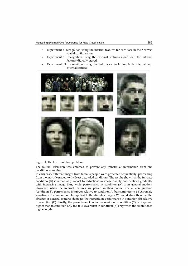
Measuring External Face Appearance for Face Classification 289
• Experiment B: recognition using the internal features for each face in their correct spatial configuration.
• Experiment C: recognition using the external features alone with the internal features digitally erased.
• Experiment D: recognition using the full faces, including both internal and external features.
Figure 1. The low resolution problem
The mutual exclusion was enforced to prevent any transfer of information from one condition to another. In each case, different images from famous people were presented sequentially, proceeding from the most degraded to the least degraded conditions. The results show that the full-face condition (D) is remarkably robust to reductions in image quality and declines gradually with increasing image blur, while performance in condition (A) is in general modest. However, when the internal features are placed in their correct spatial configuration (condition B), performance improves relative to condition A, but continues to be extremely sensitive to the amount of blur applied to the stimulus images. We can deduce then that the absence of external features damages the recognition performance in condition (B) relative to condition (D). Finally, the percentage of correct recognition in condition (C) is in general higher than in condition (A), and it is lower than in condition (B) only when the resolution is high enough.
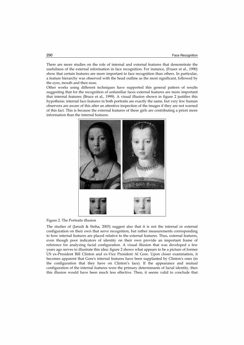
Face Recognition 290
There are more studies on the role of internal and external features that demonstrate the usefulness of the external information in face recognition. For instance, (Fraser et al., 1990) show that certain features are more important to face recognition than others. In particular, a feature hierarchy was observed with the head outline as the most significant, followed by the eyes, mouth and then nose.Other works using different techniques have supported this general pattern of results suggesting that for the recognition of unfamiliar faces external features are more important that internal features (Bruce et al., 1999). A visual illusion shown in figure 2 justifies this hypothesis: internal face features in both portraits are exactly the same, but very few human observers are aware of this after an attentive inspection of the images if they are not warned of this fact. This is because the external features of these girls are contributing a priori more information than the internal features.
Figure 2. The Portraits illusion
The studies of (Jarudi & Sinha, 2003) suggest also that it is not the internal or external configuration on their own that serve recognition, but rather measurements corresponding to how internal features are placed relative to the external features. Thus, external features, even though poor indicators of identity on their own provide an important frame of reference for analyzing facial configuration. A visual illusion that was developed a few years ago serves to illustrate this idea: figure 2 shows what appears to be a picture of former US ex-President Bill Clinton and ex-Vice President Al Gore. Upon closer examination, it becomes apparent that Gore's internal features have been supplanted by Clinton's ones (in the configuration that they have on Clinton’s face). If the appearance and mutual configuration of the internal features were the primary determinants of facial identity, then this illusion would have been much less effective. Then, it seems valid to conclude that
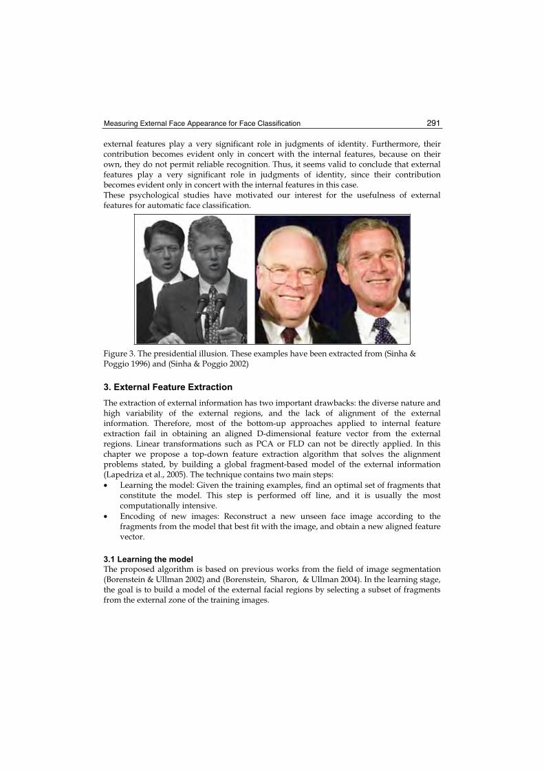
Measuring External Face Appearance for Face Classification 291
external features play a very significant role in judgments of identity. Furthermore, their contribution becomes evident only in concert with the internal features, because on their own, they do not permit reliable recognition. Thus, it seems valid to conclude that external features play a very significant role in judgments of identity, since their contribution becomes evident only in concert with the internal features in this case. These psychological studies have motivated our interest for the usefulness of external features for automatic face classification.
Figure 3. The presidential illusion. These examples have been extracted from (Sinha & Poggio 1996) and (Sinha & Poggio 2002)
3. External Feature Extraction
The extraction of external information has two important drawbacks: the diverse nature and high variability of the external regions, and the lack of alignment of the external information. Therefore, most of the bottom-up approaches applied to internal feature extraction fail in obtaining an aligned D-dimensional feature vector from the external regions. Linear transformations such as PCA or FLD can not be directly applied. In this chapter we propose a top-down feature extraction algorithm that solves the alignment problems stated, by building a global fragment-based model of the external information (Lapedriza et al., 2005). The technique contains two main steps: • Learning the model: Given the training examples, find an optimal set of fragments that
constitute the model. This step is performed off line, and it is usually the most computationally intensive.
• Encoding of new images: Reconstruct a new unseen face image according to the fragments from the model that best fit with the image, and obtain a new aligned feature vector.
3.1 Learning the model
The proposed algorithm is based on previous works from the field of image segmentation (Borenstein & Ullman 2002) and (Borenstein, Sharon, & Ullman 2004). In the learning stage, the goal is to build a model of the external facial regions by selecting a subset of fragments from the external zone of the training images.

Face Recognition 292
Image patches or fragments have been used as visual features in many recognition systems. These patches are normally extracted from images based on local properties such as similarity. A particulary useful set of features are the intermediate size image fragments, that arise in a natural way when searching for a set of features having as information as possible of the class (Ullman et al., 2002). Thus, intermediate sized image fragments are selected from a large set of candidates to represent a model of the class. This selected set is called here the Building Blocks.The learning model algorithm receives as input a training set C with images that should contain clearly visible and diverse enough external features. From this training set, we generate all the possible sub images Fi of predefined sizes and store them. This step is computationally demanding, and can be optimized by selecting fragments only from specific zones of the image. Figure 4 shows the suggested regions of interest selected in this chapter. These surrounding regions can be easily isolated with the information provided at the previous face detection step.
Figure 4. Interest’s regions of the external face features
Each fragment Fi is candidate to belong to the final model. Nevertheless, the size of the candidate set grows quadratically with the image dimensions, and the redundancy on the fragments is significant, being necessary a selection of the most representative fragments that account for the maximum diversity on the external regions. Given the facial set C and a large set of non face images C the goal is to find the fragments that are more representative of the external information of faces. The global selection criterion applied is to add to the model those fragments that can be found with high probability in face images but with low probability in non face images. The cross-correlation measure is used to determine wether a given Fragment Fi is similar to any part p from image I, and is defined as:
Fip
yxii
i
FyxFpyxpN
FpNCCσσ
−−= ,
)),()(),((1
),(

Measuring External Face Appearance for Face Classification 293
where N is the number of pixels in Fi, p and iF are the means of p and Fi respectively, and
p and Fi are their standard deviations. For each fragment Fi, we compute the maximum values of the normalized cross-correlation between Fi and each possible sub image p of I∈C ( )(CNCCi ), and in C ( )(CNCCi ).
Given a number of false positives α that can be tolerated for a fragment in C we can compute a threshold value iθ in order to assure that P( )(CNCCi )<α . This value can be used for determining wether a given fragment is present in an unseen image. Correlations below this treshold mean that not enough similarity has been found between the fragment and the image. Finally, the K fragments with highest P( )(CNCCi )>α are selected. These fragments have the highest probability to appear in the face set, and not to appear in the non face set (Borenstein & Ullman 2002, Sali & Ullman 1999) . The complete algorithm is detailed in Table 1. To ensure additional diversity on the fragment set we impose a geometrical constraint on the location of the fragments. The face image is divided in 3 independent regions: frontal part, left side and right side (see figure 4). The fragment selection process is run independently on each region, avoiding an important fragment concentration on small zones that would yield poor global reconstruction of new unseen images.
The algorithm takes as input: • The face images set C • The set C of non face images • The possible sizes of the fragments to analyze },..,{ 1 si SSS ∈
• The maximum number of fragments K that will be considered as buildingblocks.
• The predefined threshold of false positives α .1. For each fragment size iS
• Extract all the possible sub images iF of size iS from the set C using a sliding window procedure.
• Add each sub image to the candidate fragments set. • Calculate and store the normalized correlation between each
candidate fragment iS and each image from C and C .
2. Compute the threshold iθ for each fragment iF that allows at most an α false
positive ratio from the training set, (P( )(CNCCi )>iθ ) < α .
1. Compute the probability (frequency) of each fragment to describe elements from class C using the threshold
iθ , (P( )(CNCCi )>iθ ).
2. Select the K fragments with highest value P( )(CNCCi )>iθ .
Table 1. Building blocks learning algorithm

Face Recognition 294
3.2 Encoding the aligned External Information from new unseen images
Provided the learned fragment-based model of the external features, and supposing that the face detector has located a face in an image (internal features), the first step to extract the external face information is to cover the surrounding of the face area with the set of building blocks. To achieve this goal a function ),( iFINC is defined as the pixel coordinates where the maximum ),( iFpNCC for all the possible sub images Ip∈ is reached. Therefore, for each building block the place where the normalized cross-correlation value is maximum is computed, and then, the most appropriated covering is defined as an additive composition of the fragments that yields an optimal reconstruction of the surroundings of the detected internal face features. The main goal of the proposed technique is to obtain an aligned feature vector of the external information, which can be used as an input for any traditional classifier designed for learning the internal features. The following three steps perform the feature extraction: 1. Given a new unseen image x, we compute the normalized correlations between each
fragment composing the model and the area of the image that surrounds a face. We store also the position of the maximum correlation NC(I,Fi) for each fragment.
2. Using the optimal position for each fragment, a set of basis vectors B are constructed as follows: for each fragment an image of the same size as the original image is generated with the fragment set at the optimal position (obtained in the first step), and the rest of the pixels set to 0.
3. Given B, we find the coefficients S that best approximate the linear transform:
BSx ≈To compute the set of coefficients S we use the Non Negative Matrix Factorization (NMF) algorithm (Lee & Seung , 1999). The NMF algorithm fulfils the three constraints inherent to this problem: • The combination of coefficients must be additive, given that each fragment contributes
to the reconstruction of the external features. • The reconstruction error of the image external features using the fragments of the
model must be minimized, and the NMF minimizes the reconstruction error (Lee at al., 2000) in the mean squared error sense.
• The fragment set is diverse, given that is extracted from different subjects in order to model the variability of the problem. Therefore, only a small part of the fragments from the general model can be useful to reconstruct a specific face. This fact implies that the coefficients S must be sparse, and only a small part of the fragments of the model should be activated for each face.
There exist several implementations of the NMF algorithm, among them we have chosen the version developed by Patrick Hoyer (Hoyer 2004), fixing the bases matrix B to constraint the NMF to our model (Lapedriza et al., 2006). This implementation has the advantage that the sparseness coefficient can be adjusted, in order to allow or restrict the amount of fragments that take part on the reconstruction. Figure 5 shows an example of the whole feature extraction process. We use only the external regions marked to be put in correspondence with the fragment model. The reconstructed image is expressed as a linear combination between the fragments placed at the optimal position and the NMF weights. Notice that the reconstruction is not used for classification purposes. The NMF coefficients

Measuring External Face Appearance for Face Classification 295
encode the aligned feature vector that represents the external information of the face. Each feature represents the contribution of one fragment from the model in the reconstruction of the original external region.
Figure 5. Example of the reconstruction process of the external information. In the first sample the original image is plotted, and the regions where the external information is marked. Some of the fragments from the model are plotted at the optimal position under the NC criterion, and the feature extraction process is illustrated as a linear combination of this fragment-basis and a set of NMF coefficients. The resulting reconstructed image is shown.
4. Face Classification Experiments
To test this external feature extraction system we have performed different experiments, including gender, verification and subject recognition, using different classifiers. In this section we present some results showing that the proposed method allows to obtain significant information from the external zones of the face. Two publicly available databases have been used: the AR Face Database and FRGC (Face Recognition Grand Challenge, http://www.bee-biometrics.org/ ). The AR Face Database is composed of 26 face images from 126 different subjects (70 men and 56 women). The images have uniform white background. The database has from each person 2 sets of images, acquired in two different sessions, with the following structure: 1 sample of neutral frontal images, 3 samples with strong changes in the illumination, 2 samples with occlusions (scarf and glasses), 4 images combining occlusions and illumination changes, and 3 samples with gesture effects. One example of each type is plotted in figure 6.
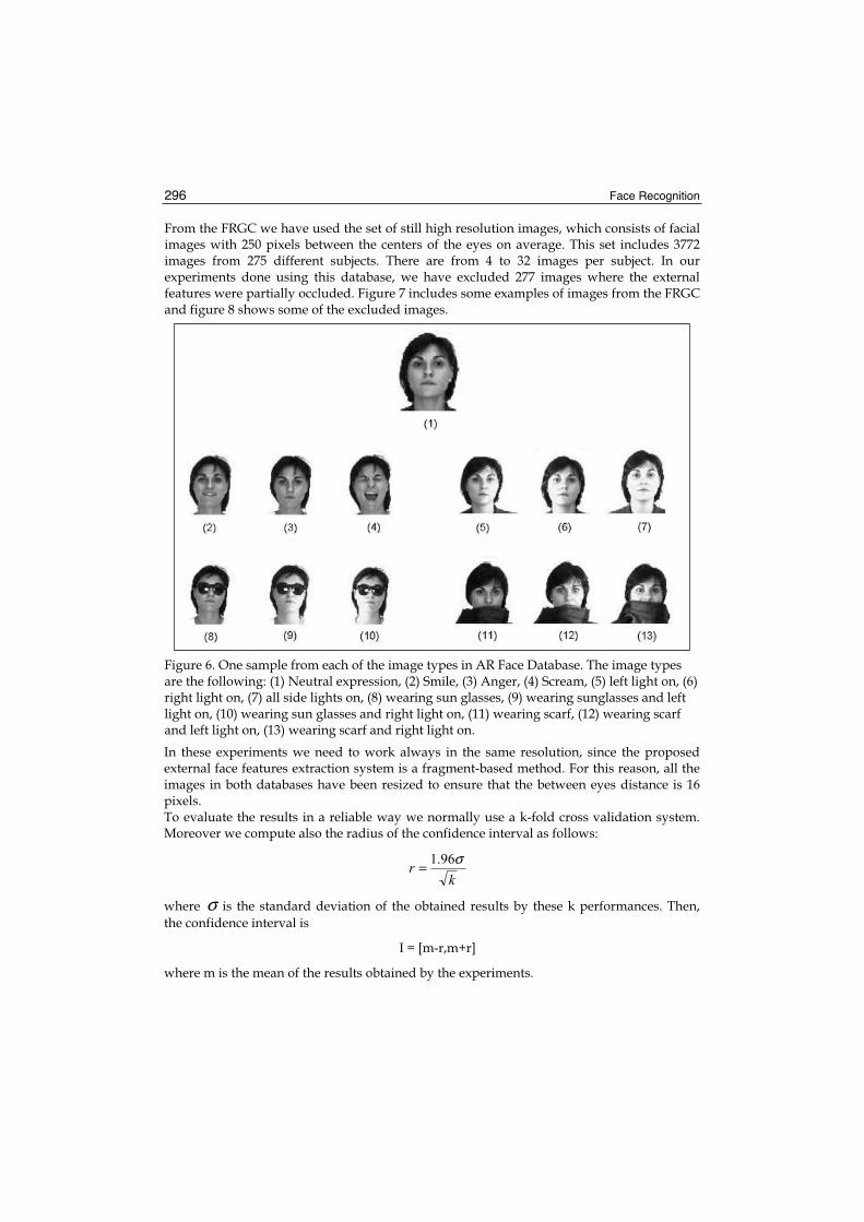
Face Recognition 296
From the FRGC we have used the set of still high resolution images, which consists of facial images with 250 pixels between the centers of the eyes on average. This set includes 3772 images from 275 different subjects. There are from 4 to 32 images per subject. In our experiments done using this database, we have excluded 277 images where the external features were partially occluded. Figure 7 includes some examples of images from the FRGC and figure 8 shows some of the excluded images.
Figure 6. One sample from each of the image types in AR Face Database. The image types are the following: (1) Neutral expression, (2) Smile, (3) Anger, (4) Scream, (5) left light on, (6) right light on, (7) all side lights on, (8) wearing sun glasses, (9) wearing sunglasses and left light on, (10) wearing sun glasses and right light on, (11) wearing scarf, (12) wearing scarf and left light on, (13) wearing scarf and right light on.
In these experiments we need to work always in the same resolution, since the proposed external face features extraction system is a fragment-based method. For this reason, all the images in both databases have been resized to ensure that the between eyes distance is 16 pixels.To evaluate the results in a reliable way we normally use a k-fold cross validation system. Moreover we compute also the radius of the confidence interval as follows:
kr σ96.1=
where σ is the standard deviation of the obtained results by these k performances. Then, the confidence interval is
I = [m-r,m+r]
where m is the mean of the results obtained by the experiments.
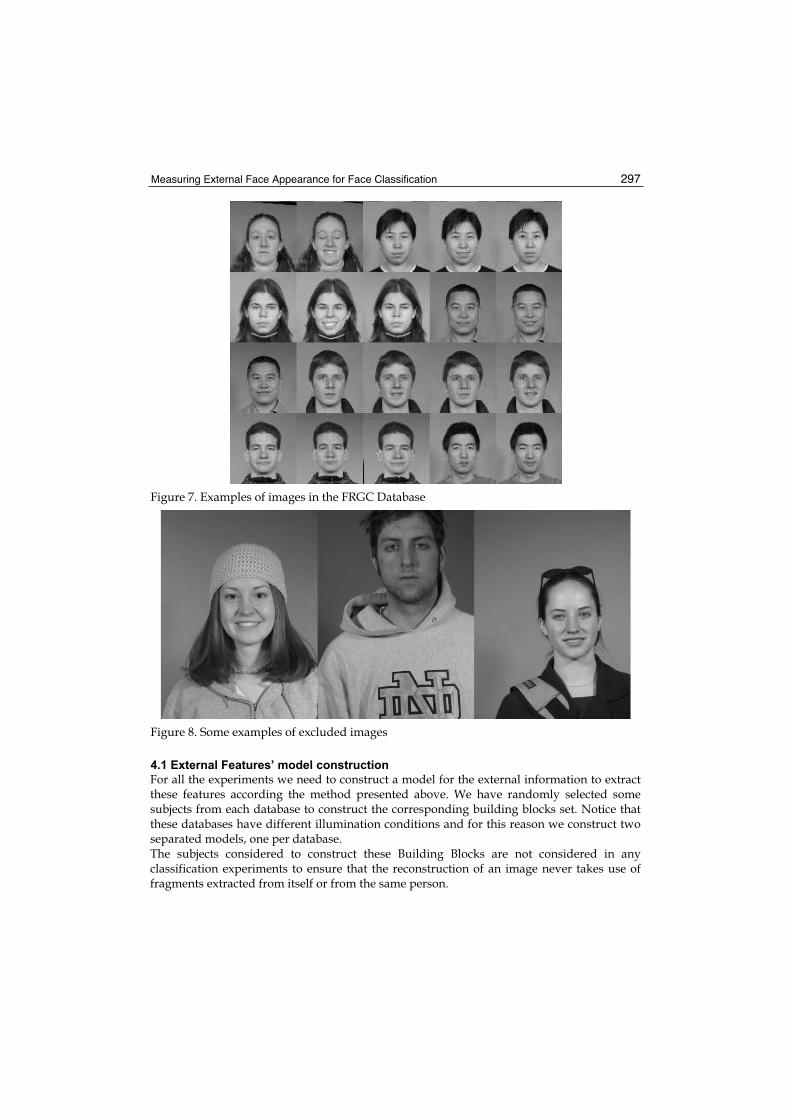
Measuring External Face Appearance for Face Classification 297
Figure 7. Examples of images in the FRGC Database
Figure 8. Some examples of excluded images
4.1 External Features’ model construction
For all the experiments we need to construct a model for the external information to extract these features according the method presented above. We have randomly selected some subjects from each database to construct the corresponding building blocks set. Notice that these databases have different illumination conditions and for this reason we construct two separated models, one per database. The subjects considered to construct these Building Blocks are not considered in any classification experiments to ensure that the reconstruction of an image never takes use of fragments extracted from itself or from the same person.

Face Recognition 298
The construction of the Building Blocks’ set follows the same protocol in both cases: • We use 80 face images from the database to extract the fragments, 40 male and 40
female.• We have automatically extracted 24 fragments of each image to construct the set of
candidate fragments and run the selection algorithm explained in section 3.1, using the parameters: α = 0.1 and K=200.
• A hundred of natural images (with no faces) extracted from the web have been selected for the C set.
4.2 Testing the external information
Here we present some results to show that the external face features contribute notably in face classification purposes. First we perform Gender recognition experiments, where the data set has been split in a training set containing the 90% of the samples and a test set with the remaining 10% from the FRGC Database. The presence of male and female samples on each set has been balanced.We have performed 50 iterations of the NMF algorithm. In these experiments we have used 5 different classifiers: Maximum Entropy, Support Vector Machines, Nearest Neighbour, Linear and Quadratic classifiers, and the accuracies have been computed in all cases as the mean of 100 repetitions (using a cross-validation strategy). The mean results of the 5 classifiers are shown in table 2.
Algorithm ME SVM NN Linear Quadratic
Accuracy 83.24 94.19 92.83 88.75 88.32
Confidence Interval 0.43 0.27 0.26 0.37 0.38
Table 2. Gender recognition experiment (FRGC)
To ensure the relevance of these external features we also perform two subject recognition experiments. In this case we have considered the same set of 2640 images as in the experiment described above. However, for the subject recognition experiment the data set has been organized as follows: a training set containing 10 randomly selected images from each subject and a test set with the remaining images. We have performed also a discriminant feature extraction on the encoded external information (NMF coefficients) and then have classified using the Nearest Neighbour (NN) . The used discriminant feature extraction technique is based on the Adaboost algorithm (Masip & Vitrià, 2005) and (Masip & Vitrià, 2006). The accuracy obtained with the NN classifier directly applied on the NMF coefficients was 43% while the best accuracy obtained using the NN classifier on the extracted features was obtained in dimensionality 315, having 56% of correctly classification. Note that these results are relevant taking into account that we consider more than 200 classes. Therefore, this shows that the external features contain enough relevant information for classification purposes.

Measuring External Face Appearance for Face Classification 299
4.3 Comparing external and internal features
To compare the contribution of external features and internal features in automatic face classification field, we perform gender recognition and subject verification experiments. First, we have selected 2210 images from the AR Face database, discarding subjects with missing images and balancing the presence of male and females. The error rates shown in this work were obtained repeating 100 times the next experimental protocol: data has been randomly split in a training and a testing set, we have used 90% of the data for training and 10% for testing; the splitting has been performed taking into account the person identity, so all samples from the same person must be in only one set to avoid person recognition instead of gender recognition. We perform the test using the maximum entropy classifier (ME). We have preformed the same gender classification experiments using only the internal features (1188 pixel values) and using only the external features (600 NMF coefficients) and the obtained rates are shown in table 3. The results obtained in the external case slightly better than the ones obtained with the internal features. This fact can be justified by the loss of information in the internal part of the face caused by the partial occlusions and the high local changes in the illumination (almost a half of the AR Face database images have occlusion artefacts, see figure 6).
ME (Confidence Interval)
Internal Features 80.4 (0.63)
External Features 82.8 (0.57)
Table 3. Gender recognition using the AR Face Database
On the other hand we have performed different subject verification experiments using internal and external features separately. The selection of the different data sets used in this experiment is based on the Sep96 FERET testing protocol (Phillips et al., 1996). In this protocol, two sets are distinguished: a target set (T), composed by the known facial images, and the query set (Q), including the unknown facial images to be identified. Two subsets should be selected from each of these sets: a gallery G⊂ T and a probe set P ⊂ Q. After this selection, the performance of the system is characterized by two statistics. The first is the probability of accepting a correct identity. This is referred as the verification probability, denoted by VP (also referred to as the hit rate in the signal detection literature). The second is the probability of incorrectly verifying a claim, that is called the false-alarm rate and is denoted by FP .We have used the LBDP (Masip & Vitrià, 2005) method to reduce the dimensionality of the data vectors, working after that in a 300-dimensionality vectorial space. We perform 2 the verification experiments using both FRGC and AR Face databases. The details of the sets used in these experiments are specified in table 4. They have been chosen following the scheme of the Lausanne Protocol configuration-1 (Kang & Taylor, 2002) and there are two kinds of subjects: clients (known by the system) and impostors (unknown by the system).
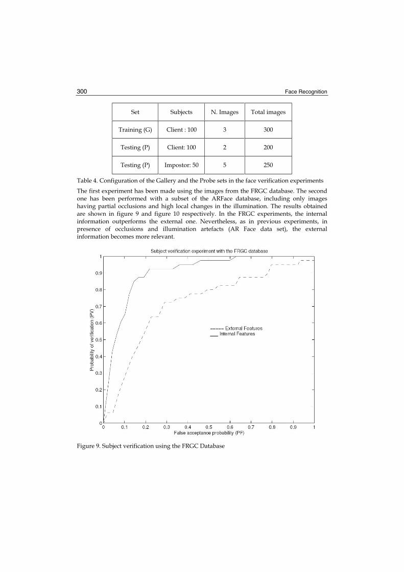
Face Recognition 300
Set Subjects N. Images Total images
Training (G) Client : 100 3 300
Testing (P) Client: 100 2 200
Testing (P) Impostor: 50 5 250
Table 4. Configuration of the Gallery and the Probe sets in the face verification experiments
The first experiment has been made using the images from the FRGC database. The second one has been performed with a subset of the ARFace database, including only images having partial occlusions and high local changes in the illumination. The results obtained are shown in figure 9 and figure 10 respectively. In the FRGC experiments, the internal information outperforms the external one. Nevertheless, as in previous experiments, in presence of occlusions and illumination artefacts (AR Face data set), the external information becomes more relevant.
Figure 9. Subject verification using the FRGC Database
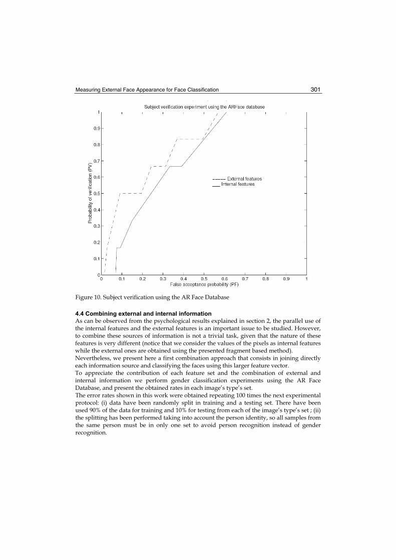
Measuring External Face Appearance for Face Classification 301
Figure 10. Subject verification using the AR Face Database
4.4 Combining external and internal information
As can be observed from the psychological results explained in section 2, the parallel use of the internal features and the external features is an important issue to be studied. However, to combine these sources of information is not a trivial task, given that the nature of these features is very different (notice that we consider the values of the pixels as internal features while the external ones are obtained using the presented fragment based method). Nevertheless, we present here a first combination approach that consists in joining directly each information source and classifying the faces using this larger feature vector. To appreciate the contribution of each feature set and the combination of external and internal information we perform gender classification experiments using the AR Face Database, and present the obtained rates in each image’s type’s set. The error rates shown in this work were obtained repeating 100 times the next experimental protocol: (i) data have been randomly split in training and a testing set. There have been used 90% of the data for training and 10% for testing from each of the image’s type’s set ; (ii) the splitting has been performed taking into account the person identity, so all samples from the same person must be in only one set to avoid person recognition instead of gender recognition.

Face Recognition 302
The results are detailed in figure 11. The best accuracy is marked with an ’*’, and the methods whose confidence intervals overlap with the best results are shown in boldface. Notice that the use of the combined feature vector (external and internal) obtains the best accuracies in almost all the cases, being the contribution of the external information more significant in presence of occlusion problems.
Figure 11. Gender recognition using the AR Face Database
5. Conclusion
In this chapter we introduce the importance of the external features in face classification problems, and propose a methodology to extract the external features obtaining an aligned feature set. The extracted features can be used as input to any standard pattern recognition classifier, as the classic feature extraction approaches dealing with internal face regions in the literature. The resulting scheme follows a top-down segmentation approach to deal with the diversity inherent to the external regions of facial images. The proposed technique is validated using two publicly available face databases in different face classification problems: gender recognition, face recognition and subject verification. In a first approach, we show that the external features encoded in the NMF coefficients yield enough useful information for classification purposes. Then we compare the information contributed by the external features and the internal features. Finally, the last step is to combine the information provided by the external and the internal features. We show that both kinds of information are complementary, providing and extra information cue that can improve the classification results in presence of occlusions and local changes in the illumination.
6. Future Work
The proposed method can be improved at three different levels: firstly the learning of the building blocks model could takes benefit from using some kind of normalization on the fragments generation. In particular, we propose the use of techniques of ridges and valleys detection to filter the images as a previous step on the feature extraction. In a second level, we plan to improve the selection of the fragments that compose the building blocs by adding a diversity measure that could model a larger rank of hairstyles. And in a third stage, we need to define a more robust combination rule of the internal and external

Measuring External Face Appearance for Face Classification 303
information. The use of ensembles of classifiers seems to be a natural continuation of this combination. For instance, the Adaboost (Freund & Schapire, 1996) algorithm can be studied for this purpose.
7. References
Borenstein, E. & Ullman, S. (2002) . Class-specific, top-down segmentation. Proceedings of the 7th European Conference on Computer Vision- Part II, pp 109-124, London, UK, 2002. Springer-Verlag.
Borenstein, E.; Sharon, E. & Ullman, S. (2004) Combining top-down and bottom-up segmentation. Proceedings of the 2004 Conference on Computer Vision and Pattern Recognition Workshop (CVPRW'04), pp 46, Washington, DC, USA, 2004. IEEE Computer Society.
Bruce, V.; Henderson, Z.; Greenwood, K.; Hancock, P. J. B.; Burton, A. M. & Miller, P. (1999) J. Exp. Psychol. Applied 5, 339-360.
Ellis, H.D. ; Shepherd, J.W. & Davies , G.M. (1979). Identification of familiar and unfamiliar faces from internal and external features: Some implications for theories of face recognition. Perception, 8:431–439, 1979.
Ellis, H. D. (1986). Face recall: A psychological perspective. Human Learning, 5, 1986. pp 189-196.
Fraser, I.H.; Craig, G.L. & Parker; D.M. (1990) Reaction time measures of feature saliency in schematic faces. Perception, 19, 1990, pp 661-673.
Freund, Y. & Schapire R. E. (1996). Experiments with a New Boosting Algorithm. Proceedings of the International Conference on Machine Learning. pp 148-156. Bari, July 1996. ISBN 1-55860-419-7, Morgan Kauffman.
Haig, N.D. (1986). Exploring recognition with interchanged facial features. Perception, 15, 1986, pp 235-247.
Hespanha, J.P; Belhumeur, P.N. & Kriegman, D.J. (1997). Eigenfaces vs fisherfaces: Recognition using class specific linear projection, IEEE Transactions on Pattern Analysis and Machine Intelligence, 19, 7 ,July 1997, 711-720.
Hoyer, P.O. (2004). Non-negative Matrix Factorization with sparseness constraints. Journal of Machine Learning Research 5. ,2004, pp 1457-1469.
Jarudi, I. N. & Sinha, P. (2003). Relative Contributions of Internal and External Features to Face Recognition. Technical Report 225. Massachusets Institute of Technology,Cambridge, MA., March 2003.
Kang T.H. & Taylor C.J. (2002). A Comparison of Face Verification Algorithms using Appearance Models. Proceedings of the 2nd Workshop on Biologically Motivated Computer Vision. vol 2, pp 477-486. Tübingen, Germany. November 2002. Springer Verlag.
Lapedriza, A.; Masip, D. & Vitrià J. (2005). Are External Face Features Useful for Automatic Face Classification?, Proceedings of the 2005 IEEE Computer Society Conference on Computer Vision and Pattern Recognition (CVPR'05) – Workshops. pp 151-159. June 2005. 0-7695-2372-2-3. San Diego, USA. IEEE Computer Society. Washington, DC, USA.
Lapedriza, A.; Masip, D. & Vitrià J. (2006). On the Use of External Face Features for Identity Verification, Journal of Multimedia. 1,4, July 2006, pp 11-20. ISSN : 1796-2048.

Face Recognition 304
Lee, D. & Seung , H. S. (1999). Learning the parts of objects with nonnegative matrix factorization, Nature, 401, July 1999, 788-791.
Lee, D. & Seung, H. S. (2000). Algorithms for Non-negative Matrix Factorization, Proceedings of Neural Information Processing Systems (NIPS), pp 556-562, (2000).
Martinez A. & Benavente, R. (1998). The AR Face database, Computer Vision Center, Tech. Rep. 24, June 1998.
Masip, D.; Kuncheva, L.I. & Vitrià, J. (2005). An ensemble-based method for linear feature extraction for two-class problems. Pattern Analysis and Applications, 8,3, pp 227-237 December 2005. Springer Verlag.
Masip, D. & Vitrià, J. (2006). Boosted discriminant projection for nearest neighbor classification. Pattern Recognition, 39, 2, February 2006, 164-170.
Peng W.; Matthew B.; Qiang Ji & Wayman J. (2005). Automatic Eye Detection and Its Validation, Proceedings of IEEE Workshop on Face Recognition Grand Challenge Experiments (with CVPR), June 2005, San Diego, CA.
Phillips P.J; Rauss, P.J & Der S.Z. (1996). FERET (Face Recognition Technology) Recognition Algorithm Development and Test Results. Technical report 995. Army Research Lab.October 1996.
Sali E. & Ullman S. (1999). Combining Class-Specific Fragments for Object Classification. Proceedings of the 10th Brittish Machine Vision Conference (BMVC), 1, 1999.
Sinha , P. & Poggio, T. I . (1996). Think I know that Face, Nature, 384, 6698, 1996, pp 404. Sinha, P. & Poggio, T. (2002) United we stand: The role of head-structure in face recognition.
Perception, 31(1):133, 2002. Turk, M. & Pentland A. (1991). Eigenfaces for recognition, Journal of Cognitive Neuroscience,
3, 1, March 1991, 71-86. Ullman, S.; Sali, E. & Vidal-Naquet, M. A. (2001). Fragment-Based Approach to Object
Representation and Classification. Proceedings of the 4th International Workshop on Visual Form, pp 85-102. May 2001.
Ullman, S.; Vidal-Naquet, M. & Sali E. (2002). Visual features of intermediate complexity and their use in classification , Nature Neuroscience, 5, 7, July 2002, 682-687.
Young, A.W.; Hay, D.C.; McWeeny, K.H.; Flude, B.M. & Ellis, A.W. (1986). Matching familiar and unfamiliar faces on internal and external features. Perception, 14, 1986, pp 737-746

16
Selection and Efficient Use of Local Features for Face and Facial Expression Recognition in a
Cortical Architecture
Masakazu Matsugu Canon Inc
Japan
1. Introduction
There are growing physiological and practical evidences that show usefulness of component (e.g., local feature) based approaches in generic object recognition (Matsugu & Cardon, 2004; Wolf et al., 2006; Mutch & Lowe, 2006; Serre et al., 2007) which is robust to variability in appearance due to occlusion and to changes in pose, size and illumination. It is no doubt clear that low level features such as edges are important and utilized in most of visual recognition tasks. However, there are only a few studies that address economical and efficient use of intermediate visual features for higher level cognitive function (Torralba et al., 2004; Opelt et al., 2006). In this chapter, inspired by cortical processing, we will address the problem of efficient selection and economical use of visual features for face recognition (FR) as well as facial expression recognition (FER). We demonstrate that by training our previously proposed (Matsugu et al., 2002) hierarchical neural network architecture (modified convolutional neural networks: MCoNN) for face detection (FD), higher order visual function such as FR and FER can be organized for shared use of such local features. The MCoNN is different from those previously proposed networks in that training is done layer by layer for intermediate as well as global features with resulting receptive field size of neurons being larger for higher layers. Higher level (e.g., more complex) features are defined in terms of spatial arrangement of lower level local features in a preceding layer. In the chapter, we will define a common framework for higher level cognitive function using the same network architecture (i.e., MCoNN) as substrate as follows. • In Section 2, we will demonstrate two examples of learning local features suitable for FD
in our MCoNN (Matsugu & Cardon, 2004). One approach is heuristic, supervised training by showing exemplar local features or patches of images, and the other is unsupervised training using SOM (self-organizing map) combined with supervised training in MCoNN.
• In the proposed framework, both FR and FER utilize common local features (e.g., corner like end-stop structures) learnt from exemplary image fragments (e.g., mouth corners, eye-corners) for FD. Specifically, in Section 3, spatial arrangement information of such local features is extracted implicitly for FR as feature vectors used in SVM classifiers (Matsugu et al., 2004). In the case of FER described in Section 4, spatial arrangement of

Face Recognition 306
common local features is used explicitly for rule-based analysis (Matsugu et al., 2003). We will show, by simulation, that learnt features for FD turn out to be useful for FR and FER as well.
2. Learning Local Features for Generic Object Detection
2.1 Modified convolutional neural network (MCoNN)
Convolutional neural networks (CoNN), with hierarchical feed-forward structure, consist of feature detecting (FD) layers, each of which followed with a feature pooling (FP) layer or sub-sampling layer. CoNN (LeCun and Bengio, 1995) as well as Neocognitrons (Fukushima, 1980) have been used for face detection (Matsugu et al., 2002; Osadchy et al., 2004) and recognition (Lawrence et al., 1995).
Figure 1. Modified convolutional neural network (MCoNN) architecture for facedetection
Proposed architecture in Figure 1 comes with the property of robustness in object recognition such as translation and deformation invariance as in well-known neocognitrons,which also have similar architecture. The MCoNN contains the same three properties as the original CoNN as well as Neocognitrons: local receptive fields, shared weights, and alternating feature detection/pooling mechanism to detect some intermediate (in the sense that local but not too simple) local features. Those properties are can be widely found in cortical structures (Serre et al., 2005). Feature pooling (FP) neurons perform either maximum value detection as in Riesenhuber & Poggio (1999) and Serre et al. (2007) or local averaging in their receptive fields of appropriate size. Our model (MCoNN) for face detection as shown in Figure 1 is different from traditional ones in many aspects. First, it has only FD modules in the bottom and top layers. The intermediate features detected in FD2 constitute a set of figural alphabets (Matsugu et al., 2002; Matsugu & Cardon, 2004). Local features in FD1 are used as bases of figural alphabets, which are used for eye or mouth detection. Face detecting module in the top layer is fed

Selection and Efficient Use of Local Features for Face and Facial Expression Recognition in a Cortical Architecture 307
with a set of outputs from facial component (e.g., such as eye, mouth) detectors as spatially ordered set of local features of intermediate complexity. Second, we do not train FP (or sub-sampling) layers (FP neurons perform either maximum value detection or local averaging in their receptive fields). Third, we use a detection result of skin color area as input to the face detection module in FD4. The skin area is obtained simply by thresholding of hue data of input image in the range of [-0.078,0.255] for the full range of [-0.5,0.5], which is quite broad indicating that skin color feature plays merely auxiliary part in the proposed system. Third, in our MCoNN model, in contrast to the original CoNN, local features to be detected in respective layers are pre-defined, and trained module by module (i.e., for each local feature class) for specifi category of local features; edge-like features in the first layer, and then in the second layer, corner-like structures (i.e., ‘<’ and ‘>’ end-stop), elongated blobs (i.e., upper part bright blob, and lower part bright blob) are detected. The second and third layers are composed of feature detecting layer and feature pooling layer as in original CoNN and Neocognitrons. Local features detected in the second layer constitute some alphabetical local features in our framework, and details will be explained in the next section. Eye and mouth features are detected in the third layer. Finally, a face is detected in the forth layer using outputs from the third layer and skin area data defined by some restricted range of hue and saturation values. The training proceeds as follows. As in (Matsugu et al., 2002, Mitarai et al., 2003), training of the MCoNN is performed module by module using fragment images as positive data extracted from publicly available database (e.g., Softpia Japan) of more than 100 persons. Other irrelevant fragment images extracted from background images are used as negative samples. In the first step, two FD layers from the bottom, namely FD1 with 8 modules and FD2 with 4 modules, are trained using standard back-propagation with intermediate local features (e.g., eye corners) as positive training data sets. Negative examples that do not constitute the corresponding feature category are also used as false data. Specifically, we trained the FD2 layer, the second from the bottom FD layer to form detectors of intermediate features, such as end-stop structures or blobs (i.e., end-stop structures for left and right side and two types of horizontally elongated blobs (e.g., upper part bright, lower part bright) with varying sizes, rotation (up to 30 deg. with rotation in-plane axis as well as head axis). These features for training are fragments extracted from face images. More complex local feature detectors (e.g., eye, mouth detectors, but not restricted to these) are trained in the third or fourth FD layer using the patterns extracted from transforms as in the FD2 layer. As a result of these training sequences, the top FD layer, FD4, learns to locate faces in complex scenes. The size of partial images for the training is set so that only one class of specific local feature is contained. The number of training data set is 14847 including face images and background image for FD4 module, 5290 for FD3, and 2900 for FD2.
2.2 Supervised learning of local features as figural alphabets in MCoNN
Selecting optimal local features for multi-class object detection (Papageorgiou et al, 1998) is a crucial step toward generic object recognition. Face detection, face recognition, and facial expression recognition are no exceptions. In Burl et al. (1995) and Weber et al. (2000), an interest point operator and a k-means clustering algorithm are used to extract and regroup high-level features for estimating the parameters of the underlying probabilistic model.
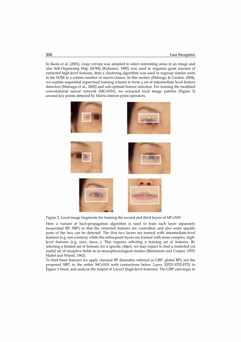
Face Recognition 308
In Ikeda et al. (2001), image entropy was adopted to select interesting areas in an image and also Self-Organizing Map (SOM) (Kohonen, 1985) was used to organize great amount of extracted high-level features, then a clustering algorithm was used to regroup similar units in the SOM to a certain number of macro-classes. In this section (Matsugu & Cardon, 2004), we explain sequential supervised training scheme to form a set of intermediate level feature detectors (Matsugu et al., 2002) and sub-optimal feature selection. For training the modified convolutional neural network (MCoNN), we extracted local image patches (Figure 2) around key points detected by Harris interest point operators.
Figure 2. Local image fragments for training the second and third layers of MCoNN
Here a variant of back-propagation algorithm is used to train each layer separately (sequential BP: SBP) so that the extracted features are controlled, and also some specific parts of the face can be detected. The first two layers are trained with intermediate-level features (e.g. eye-corners), while the subsequent layers are trained with more complex, high-level features (e.g. eyes, faces...). This requires selecting a training set of features. By selecting a limited set of features for a specific object, we may expect to find a restricted yet useful set of receptive fields as in neurophysiological studies (Blackmore and Cooper, 1970; Hubel and Wiesel, 1962). To find these features we apply classical BP (hereafter referred as GBP: global BP), not the proposed SBP, to the entire MCoNN with connections below Layer 2(FD1-FD2-FP2) in Figure 3 fixed, and analyze the output of Layer3 (high-level features). The GBP converges to

Selection and Efficient Use of Local Features for Face and Facial Expression Recognition in a Cortical Architecture 309
a local minimum, therefore the algorithm will tend to extract sub-optimal features to minimize the detection error. To examine the validity of our scheme of using MCoNN trained by GBP for generic object detection, we applied the MCoNN for face detection to the detection of bright-colored cars with significant variance in shape, illumination, size and orientation. The size of the images used for learning was 156 x 112, and 90 images were used for training and 10 images for validation. We aimed to find characteristic high-level features for the detection of this type of objects under particular view. In addition, it was necessary to tailor our model to be able to distinguish between cars and other rectangular objects. For this reason, we included a set of negative non-car examples, with similar rectangular shape but which were not cars.
2.3 Unsupervised learning of local features as figural alphabets in MCoNN
In this section (Matsugu & Cardon, 2004), we present an unsupervised feature extracting and clustering procedure, using an interest operator combined with a SOM. In contrast with Opelt et al. (2006), we do not use AdaBoost framework for this task. Instead, proposed method combines the advantages of both Weber et al. (2000) and Ikeda et al. (2001) by selecting a limited number of features and regrouping them using a topographic vector quantizer (SOM); acting like a vector quantizer and introducing a topographic relation at the same time. The obtained feature classes are self-organized, low-and intermediate-level features that are used to train the two first layers of the MCoNN and obtain a minimum set of alphabetical receptive fields. Those alphabets as in Opelt et al. (2006) considerably reduces the complexity of the network by decreasing the number of parameters and can be used for detection of different object classes (e.g. faces, cars,...). We also introduce a method to select optimal high-level features and illustrate it with the car detection problem. The whole network for face detection as well as car detection is described in the lower part of Figure 3. Some specific local fragments of image extracted a priori, by using the proposed method in this study, are used to train the first two layers of the MCoNN. First, we train the MCoNN to recognize only one feature (one output plane in FD2). A sequential back-propagation algorithm (Matsugu et al., 2002) is used for learning and weights are updated after each training pattern (fragments of images) is presented. A fixed number of 100 epochs has been used. For each training set, a different number of cell-planes in layer S1 have been tested. The network has essentially four distinct sets of layers: FD1, FD2-FP2, FD3-FP3, FD4 (FDk: the kth feature detecting layer; FPj: the jth feature pooling layer for subsampling). Layers FD3-FP3 and above are concerned with object specific feature detection. In order to limit the number of features to object-relevant features, an interest point operator is used. This operator selects corner-like features in the image. Having selected a restricted number of points using keypoint detector (Harris & Stephens, 1988; Lowe, 1999;Kadir & Brady, 2001; Csurka et al. 2004) we extract features around these points. These features are used as learning set for the SOM well suited for classifying and visualizing our feature set. It turned out that the illumination has a big influence on the classification of our features, so we have rescaled the feature set between -1 and 1 before applying the SOM. Each unit of the SOM defines a training set for the MCoNN. Once lower-level alphabetical feature detectors are formed, higher level feature detectors can be obtained from BP with connections between neurons below intermediate layers fixed. Since we are interested in low-level features to train the first two layers of the MCoNN, we
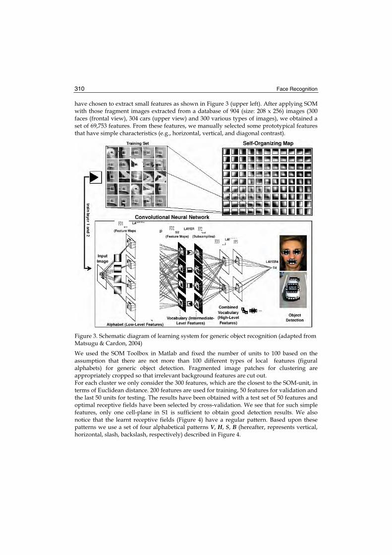
Face Recognition 310
have chosen to extract small features as shown in Figure 3 (upper left). After applying SOM with those fragment images extracted from a database of 904 (size: 208 x 256) images (300 faces (frontal view), 304 cars (upper view) and 300 various types of images), we obtained a set of 69,753 features. From these features, we manually selected some prototypical features that have simple characteristics (e.g., horizontal, vertical, and diagonal contrast).
Figure 3. Schematic diagram of learning system for generic object recognition (adapted from Matsugu & Cardon, 2004)
We used the SOM Toolbox in Matlab and fixed the number of units to 100 based on the assumption that there are not more than 100 different types of local features (figural alphabets) for generic object detection. Fragmented image patches for clustering are appropriately cropped so that irrelevant background features are cut out. For each cluster we only consider the 300 features, which are the closest to the SOM-unit, in terms of Euclidean distance. 200 features are used for training, 50 features for validation and the last 50 units for testing. The results have been obtained with a test set of 50 features and optimal receptive fields have been selected by cross-validation. We see that for such simple features, only one cell-plane in S1 is sufficient to obtain good detection results. We also notice that the learnt receptive fields (Figure 4) have a regular pattern. Based upon these patterns we use a set of four alphabetical patterns V, H, S, B (hereafter, represents vertical, horizontal, slash, backslash, respectively) described in Figure 4.
FD1FD2 FP2
FD3 FP3

Selection and Efficient Use of Local Features for Face and Facial Expression Recognition in a Cortical Architecture 311
We observe that some feature clusters in the SOM have a more complex aspect as shown in Figure 3. We claim that these more complex features can be detected using the simple receptive fields, described in the previous section. Considering for example the feature described in Figure 3, we see that this eye-corner type feature can be decomposed into two local alphabetical features (Figure 5). The usefulness of our alphabetical set appears when we want to detect, using a small number of receptive fields, a bit more higher-level features with more complex geometrical or textual structures. Let us consider the features used to detect a complete eye or a mouth (Matsugu et al., 2002). They can be decomposed to two horizontal, two slash and two back-slash components (Figure 6).
Figure 4. Alphabetical patterns obtained from SOM which are used for training McoNN. Resuling receptive fields of McoNN correspond to each feature detector
With a limited set of three fixed receptive fields H, S and B it turned out that we reach a detection rate of eye-corner comparable to that of using six learnt receptive fields. Our alphabetical set, being close to the optimal set of weights, therefore outperforms the learnt weights. We can extend these results for different types of complex features and construct a vocabulary set that can be recognized with H, V, S, and B. For illustration purposes, we have tested our alphabet with images from which features have been extracted. It turned out that we could detect, in the S2 layer, eye- and mouth-corners as well as the side mirrors of a car, using only three receptive fields (H, S and B).
Figure 5. Example (corner-like structure) of local feature extracted from local image patches of eye as a figural alphabet and its decomposition into three elementary features
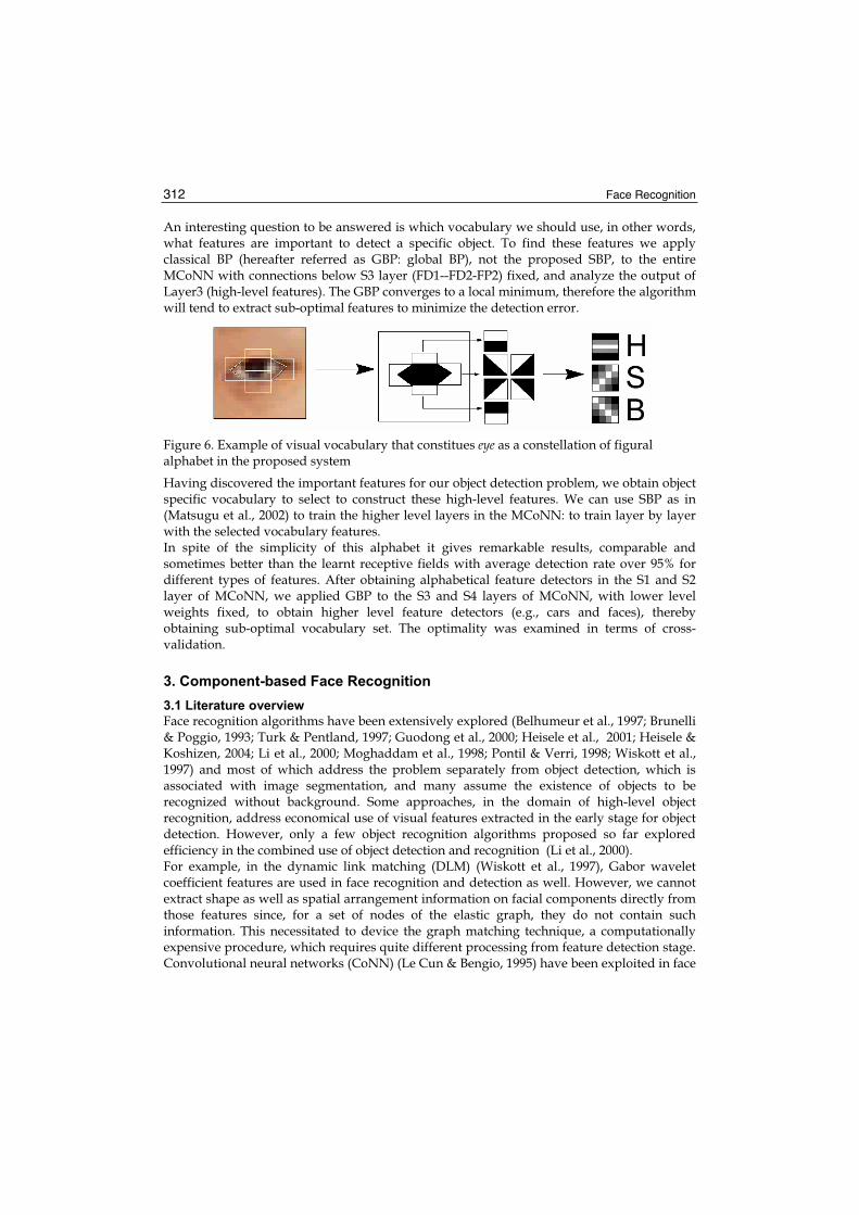
Face Recognition 312
An interesting question to be answered is which vocabulary we should use, in other words, what features are important to detect a specific object. To find these features we apply classical BP (hereafter referred as GBP: global BP), not the proposed SBP, to the entire MCoNN with connections below S3 layer (FD1--FD2-FP2) fixed, and analyze the output of Layer3 (high-level features). The GBP converges to a local minimum, therefore the algorithm will tend to extract sub-optimal features to minimize the detection error.
Figure 6. Example of visual vocabulary that constitues eye as a constellation of figural alphabet in the proposed system
Having discovered the important features for our object detection problem, we obtain object specific vocabulary to select to construct these high-level features. We can use SBP as in (Matsugu et al., 2002) to train the higher level layers in the MCoNN: to train layer by layer with the selected vocabulary features. In spite of the simplicity of this alphabet it gives remarkable results, comparable and sometimes better than the learnt receptive fields with average detection rate over 95% for different types of features. After obtaining alphabetical feature detectors in the S1 and S2 layer of MCoNN, we applied GBP to the S3 and S4 layers of MCoNN, with lower level weights fixed, to obtain higher level feature detectors (e.g., cars and faces), thereby obtaining sub-optimal vocabulary set. The optimality was examined in terms of cross-validation.
3. Component-based Face Recognition
3.1 Literature overview
Face recognition algorithms have been extensively explored (Belhumeur et al., 1997; Brunelli & Poggio, 1993; Turk & Pentland, 1997; Guodong et al., 2000; Heisele et al., 2001; Heisele & Koshizen, 2004; Li et al., 2000; Moghaddam et al., 1998; Pontil & Verri, 1998; Wiskott et al., 1997) and most of which address the problem separately from object detection, which is associated with image segmentation, and many assume the existence of objects to be recognized without background. Some approaches, in the domain of high-level object recognition, address economical use of visual features extracted in the early stage for object detection. However, only a few object recognition algorithms proposed so far explored efficiency in the combined use of object detection and recognition (Li et al., 2000). For example, in the dynamic link matching (DLM) (Wiskott et al., 1997), Gabor wavelet coefficient features are used in face recognition and detection as well. However, we cannot extract shape as well as spatial arrangement information on facial components directly from those features since, for a set of nodes of the elastic graph, they do not contain such information. This necessitated to device the graph matching technique, a computationally expensive procedure, which requires quite different processing from feature detection stage. Convolutional neural networks (CoNN) (Le Cun & Bengio, 1995) have been exploited in face

Selection and Efficient Use of Local Features for Face and Facial Expression Recognition in a Cortical Architecture 313
recognition and hand-written character recognition. In (Matsugu et al., 2001, 2002), we proposed a MCoNN model for robust face detection. SVM has also been used for face recognition (Guodong et al., 2000; Heisele et al., 2001; Heisele & Koshizen, 2004; Li et al., 2000; Pontil & Verri, 1998). In particular, in (Heisele et al., 2001; Heisele & Koshizen, 2004), SVM classification was used for face recognition in the component-based approach. This section, in the domain of face recognition as a case study for general object recognition with object detection, explores the direct use of intermediate as well as low level features obtained in the process of face detection. Specifically, we explore the combined use of our MCoNN and support vector machines (SVM), the former used for feature vector generation, the latter for classification. Proposed algorithm is one of component-based approaches (Heisele et al., 2001; Heisele & Koshizen, 2004) with appearance models represented by a set of local, area-based features. The direct use of intermediate feature distributions obtained in face detection, for face recognition, brings unified and economical process that involves simple weighted summation of signals, implemented both in face detection and recognition.
3.2 Proposed component based face recognition
Proposed face recognition system (Matsugu et al., 2004) utilizes intermediate features extracted from face detection system using MCoNN, which are fed to SVM for classification. This combination of MCoNN with SVM is similar in spirit to recent works by Serre et al. (2007) and Mutch & Lowe (2006). Figure 7 shows detailed structure of the MCoNN for face detection as well as face recognition. Here, we describe feature vectors and the procedure for their generation in face recognition. A feature vector, F, used in SVM for face recognition is an N dimensional vector, synthesized from a set of local output distributions, F1 (as shown in Figure 2(1)), in a module detecting edge-like feature in FD1 layer in addition to output distributions, F2, (as shown in Figure 2(2)) of two intermediate-level modules detecting eye and mouth in FD2 layer. Thus, F = (F1, F2) where F1 = (F11, …, F1m) and F2 = (F21, …, F2n) are synthesized vectors formed by component vectors, F1k (k=1, ..., m) and F2k (k=1, ..., n), respectively.Each component vector represents possibility or presence of specific class of local feature in an assigned local area. Dimension of a component vector is the area of a rectangular region as in Figure 9. Thus dimension of feature vector, N, is the total summation of respective dimensions of component vectors. In particular, F1 =(F11, F12, …, F1,15), and local areas, total number of assigned areas being 15 as in Figure 9 (1), for component vectors are set around eye, nose, and mouth, using the detected eye location from the MCoNN. F1 reflects shape information of eye, mouth, and nose. F2 = (F21, F22, F23), and each component vector reflects spatial arrangement of eye or eye and nose, etc., depending on how local areas in FD2 (e.g., positions and size) are set. The procedure for feature vector generation is summarized as follows. First, we define a set of local areas for FD1 as well as FD3 modules based on the CNN output in FD3 modules for eye and mouth detection. Positions of local areas in FD1 module are set around specific facial components (i.e., eyes, mouth) as illustrated in Figure 9 (1). The size of respective local areas in the output plane of FD1 module is set relatively small (e.g., 11 x 11) so that local shape information of figural alphabets can be retained in the output distribution, while the local area in the FD2 plane is relatively larger (e.g., 125 x 65) so that information concerning spatial arrangement of facial components (e.g., eye) is reflected in the distribution of FD2 outputs.

Face Recognition 314
FD1
FD2 FP2
FD3
FP3
FD4
First Layer
Second Layer Third Layer
Fourth Layer
Input Layer
FP4
FD4’
Input Image
Skin Area
Second Face
Detection
Modules
Figure 7. MCoNN for face recognition and facial expression recognition. Outputs from encircled modules in FD1 and FD2 layers are used for face recognition
Figure 8. Intermediate output from MCoNN (1):input image, (2) output example from FD1, (3) intermediate outputs from encircled modules of FD2 in Figure 7
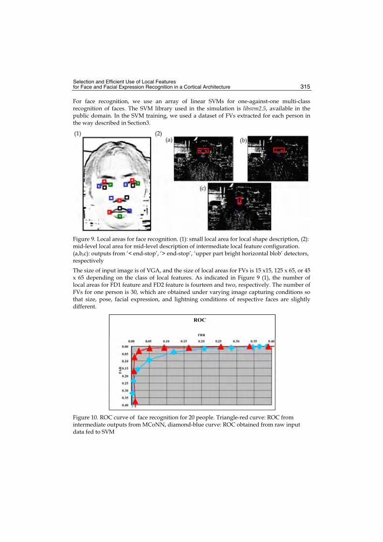
Selection and Efficient Use of Local Features for Face and Facial Expression Recognition in a Cortical Architecture 315
For face recognition, we use an array of linear SVMs for one-against-one multi-class recognition of faces. The SVM library used in the simulation is libsvm2.5, available in the public domain. In the SVM training, we used a dataset of FVs extracted for each person in the way described in Section3.
Figure 9. Local areas for face recognition. (1): small local area for local shape description, (2): mid-level local area for mid-level description of intermediate local feature configuration. (a,b,c): outputs from ‘< end-stop’, ‘> end-stop’, ‘upper part bright horizontal blob’ detectors, respectively
The size of input image is of VGA, and the size of local areas for FVs is 15 x15, 125 x 65, or 45 x 65 depending on the class of local features. As indicated in Figure 9 (1), the number of local areas for FD1 feature and FD2 feature is fourteen and two, respectively. The number of FVs for one person is 30, which are obtained under varying image capturing conditions so that size, pose, facial expression, and lightning conditions of respective faces are slightly different.
Figure 10. ROC curve of face recognition for 20 people. Triangle-red curve: ROC from intermediate outputs from MCoNN, diamond-blue curve: ROC obtained from raw input data fed to SVM

Face Recognition 316
Face image database used ofr training and testing is in-house DB (10 subjects, 1500 images) and PIE database (we used part of the DB: 15 subjects 60 images) by CMU. We compared results obtained from McoNN’s intermediate outputs with those obtained from raw data using the same local area as in Figure 9. ROC curves in Figure 10 obtained for in-house face database show that using intermediate outputs rather than raw data provide better performance. Using the same dataset, we compared our model with commercially available software which is based on DLM (Wiskott et al., 1997). The recognition rate turned out to be almost the same for the relative size of 0.8 to 1.2, while F.A.R. is slightly inferior to our model (i.e., F.A.R. is not perfectly zero), suggesting that our model involving much simpler operations equals to the performance of one of the best models (Matsugu et al., 2004).
4. Component-based Facial Expression Recognition
4.1 Literature overview
Facial expressions as manifestations of emotional states, in general, tend to be different among individuals. For example, smiling face as it appears may have different emotional implications for different persons in that ‘smiling face’, perceived by others, for some person does not necessarily represent truly smiling state for that person. Only a few algorithms (e.g., Ebine & Nakamura, 1999) have addressed robustness to such individuality in facial expression recognition. Furthermore, in order for facial expression recognition (FER) to be used for human-computer-interaction, for example, that algorithm must have good ability in dealing with variability of facial appearance (e.g., pose, size, and translation invariance). Most algorithms, so far, have addressed only a part of these problems (Wallis & Rolls, 1997). In this study, we propose a system for facial expression recognition that is robust to variability that originates from individuality and viewing conditions. Recognizing facial expression under rigid head movements was addressed by (Black & Yacoob, 1995). Neural network model that learns to recognize facial expressions from an optical flow field was reported in (Rosenblum et al., 1996). Rule-based system was reported in (Yacoob & Davis, 1996) and (Black & Yacoob, 1997), in which primary facial features were tracked throughout the image sequence. Recently, Fasel (2002) has proposed a model with two independent convolutional neural networks, one for facial expression and the other for face identity recognition, which are combined by an MLP.
4.2 Facial expression recognition using local features extracted by MCoNN
We show, in this section, proposed rule-based processing scheme to enhance subject independence in facial expression recognition. We found that some of lower level features extracted by the first FD layer of MCoNN for face detection as well as face recognition are also useful for facial expression recognition. Primary features used in our model are horizontal line segments made up of edge-like structures similar to step and roof edges (extracted by two modules in FD1 layer, circled in Figure 7 representing parts of eyes, mouth, and eyebrows. For example, changes in distance between end-stops (e.g., left-corner of left eye and left side end-stop of mouth) within facial components and changes in width of line segments in lower part of eyes or cheeks are detected to obtain saliency scores of a specific facial expression. Primary cues related to facial actions adopted in our facial analysis for the detection of smiling/laughing faces are as follows. 1. Distance between endpoints of eye and mouth gets shorter (lip being raised)
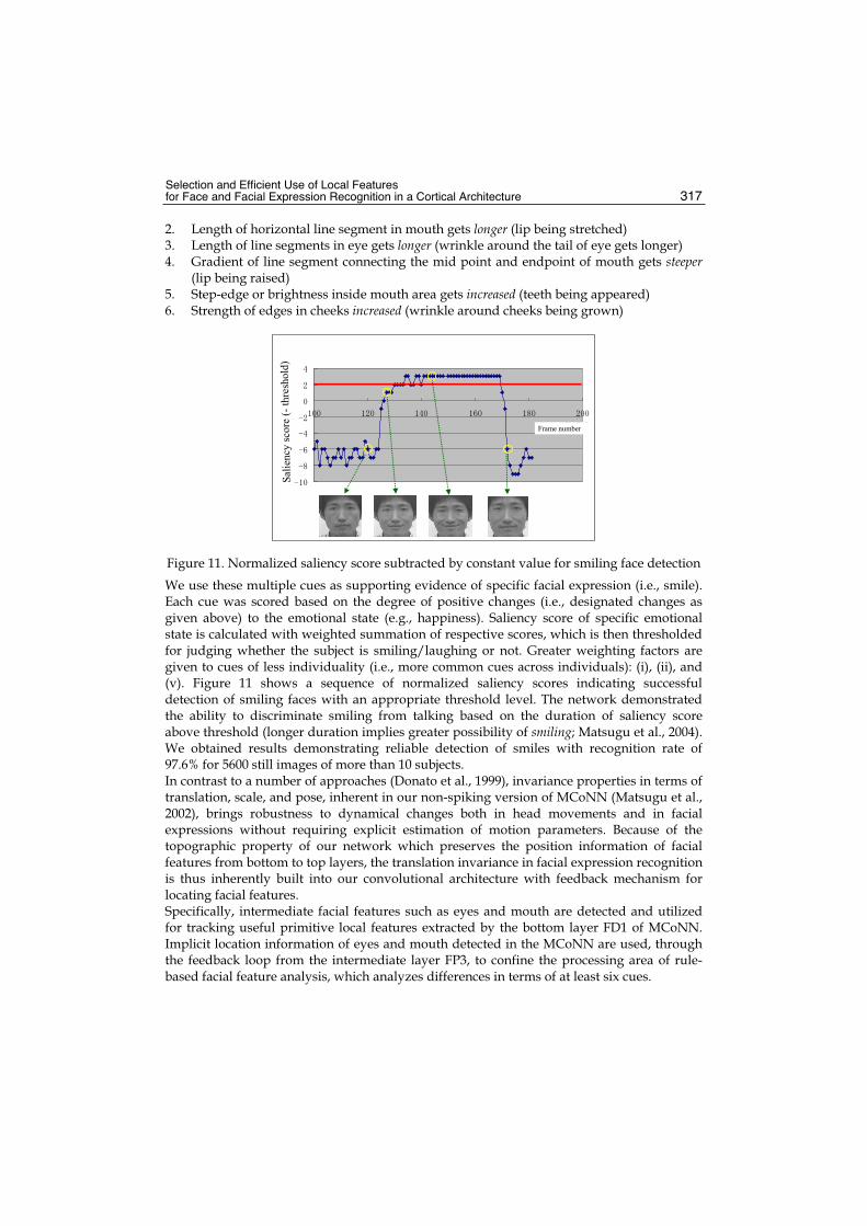
Selection and Efficient Use of Local Features for Face and Facial Expression Recognition in a Cortical Architecture 317
2. Length of horizontal line segment in mouth gets longer (lip being stretched) 3. Length of line segments in eye gets longer (wrinkle around the tail of eye gets longer) 4. Gradient of line segment connecting the mid point and endpoint of mouth gets steeper
(lip being raised) 5. Step-edge or brightness inside mouth area gets increased (teeth being appeared) 6. Strength of edges in cheeks increased (wrinkle around cheeks being grown)
Frame number
Sal
iency
score
(-th
resh
old
)
Figure 11. Normalized saliency score subtracted by constant value for smiling face detection
We use these multiple cues as supporting evidence of specific facial expression (i.e., smile). Each cue was scored based on the degree of positive changes (i.e., designated changes as given above) to the emotional state (e.g., happiness). Saliency score of specific emotional state is calculated with weighted summation of respective scores, which is then thresholded for judging whether the subject is smiling/laughing or not. Greater weighting factors are given to cues of less individuality (i.e., more common cues across individuals): (i), (ii), and (v). Figure 11 shows a sequence of normalized saliency scores indicating successful detection of smiling faces with an appropriate threshold level. The network demonstrated the ability to discriminate smiling from talking based on the duration of saliency score above threshold (longer duration implies greater possibility of smiling; Matsugu et al., 2004). We obtained results demonstrating reliable detection of smiles with recognition rate of 97.6% for 5600 still images of more than 10 subjects. In contrast to a number of approaches (Donato et al., 1999), invariance properties in terms of translation, scale, and pose, inherent in our non-spiking version of MCoNN (Matsugu et al., 2002), brings robustness to dynamical changes both in head movements and in facial expressions without requiring explicit estimation of motion parameters. Because of the topographic property of our network which preserves the position information of facial features from bottom to top layers, the translation invariance in facial expression recognition is thus inherently built into our convolutional architecture with feedback mechanism for locating facial features. Specifically, intermediate facial features such as eyes and mouth are detected and utilized for tracking useful primitive local features extracted by the bottom layer FD1 of MCoNN. Implicit location information of eyes and mouth detected in the MCoNN are used, through the feedback loop from the intermediate layer FP3, to confine the processing area of rule-based facial feature analysis, which analyzes differences in terms of at least six cues.

Face Recognition 318
It turned out that the system is quite insensitive to individuality of facial expressions with the help of the proposed rule-based processing using single but individual normal face. Because of the voting of scores for various cues in terms of differences of facial features in neutral and emotional states, individuality is averaged out to obtain subject independence.
5. Conclusion
In this chapter, we reviewed our previously proposed leaning methods (unsupervised and supervised) for appropriate and shared (economical) local feature selection and extraction for generic face related recognition. In particular, we demonstrated feasibility of our hierarchical, component based visual pattern recognition model, MCoNN, as an implicit constellation model in terms of convolutional operation of local feature, providing a substrate for generic object detection/recognition. Detailed simulation study showed that we can realize face recognition as well as facial expression recognition efficiently and economically with satisfactory performances by using the same set of local features extracted from the MCoNN for face detection.
6. Acknowledgement
We used a face database HOIP by Softpia Japan to train the network for face detection.
7. References
Belhumeur, P., Hesoanha, P. & Kriegman, D. (1997). Eigenfaces vs fisherfaces: recognition using class specific linear projection, IEEE Trans. on Pattern Analysis and Machine Intelligence, vol. 19, 711-720
Black, M. & Yacoob, Y. (1995). Tracking and recognizing rigid and non-rigid facial motions using local parametric models of image motion, Proc. IEEE Fifth Int. Conf. on Computer Vision, 374-381
Black, M. & Yacoob, Y. (1997). Recognizing Facial Expressions in Image Sequences Using Local Parameterized Models of Image Motion, Int. J. of Computer Vision, vol. 25, 23-48
Blackmore, C. & Cooper, G. E. (1970). Development of the brain depends on the visual environment, Nature, vol. 228, 477-478
Brunelli, R. & Poggio T. (1993). Face recognition: features versus templates, IEEE Trans. on Pattern Analysis and Machine Intelligence, vol. 15, 1042-1052
Burl, M., Leung, T. & Perona, P. (1995). Face localization via shape statistics, Proc. Intl. Workshop on Automatic Face and Gesture Recognition
Csurka, G., Dance, C. R., Fan, L., Willamowski, J. & Bray, C. (2004). Visual categorization with bags of keypoints, Proc. European Conf. On Computer Vision, Springer-Verlag, Berlin
Donato, G., Bartlett, M. S., Hager, J. C., Ekman, P. & Sejnowski, T. (1999). Classifying facial actions, IEEE Trans. Pattern Analysis and Machine Intelligence, vol.21, 974-989
Ebine, H. & Nakamura, O. (1999). The recognition of facial expressions considering the difference between individuality (in Japanese), Trans. IEE of Japan, vol.119-C, 474-481
Fasel, B. (2002). Robust face analysis using convolutional neural networks, Proc. Int. Conf. on Pattern Recognition
Fergus, R., Perona, P. & Zisserman, A. (2003). Object class recognition by unsupervised scale-invariant learning, Proc. IEEE Int. Conf. On Computer Vision and Pattern Recognition

Selection and Efficient Use of Local Features for Face and Facial Expression Recognition in a Cortical Architecture 319
Földiák, P. (1991). Learning invariance from transformation sequences, Neural Comput. vol. 3, 194-200
Fukushima, K. (1980). Neocognitron: a self-organizing neural networks for a mechanism of pattern recognition unaffected by shift in position. Biological Cybernetics vol. 36, 193-202
Guodong, G., Li, S. & Kapluk, C. (2000). Face recognition by support vector machines. Proc. IEEE International Conf. On Automatic Face and Gesture Recognition, 196-201
Harris, C. & Stephens, M. (1988). A combined corner and edge detector, Proc. Alvey Vision Conf. 147-151
Heisele, B., Ho, P. & Poggio, T. (2001). Face recognition with support vector machines: global versus component-based approach. Proc. International Conf. on Computer Vision, 688-694
Heisele, B. & Koshizen, T. (2004). Components for face recognition Proc. IEEE International Conf. on Automatic Face and Gesture Recognition
Hubel D. & Wiesel T. (1962). Receptive fields, binocular interaction and functional architecture in the cat’s visual cortex. Journal of Physiology vol. 160, 106-154
Ikeda, H., Kashimura, H., Kato, N. & Shimizu, M. (2001). A novel autonomous feature clustering model for image recognition, Proc. of the 8th International Conference on Neural Information Processing
Kadir, T. & Brady, M. (2001). Scale, saliency and image description, International Journal of Computer Vision, vol. 45, 83-105
Kohonen, T. (1985). Self-Organizing Maps. Springer-Verlag, Berlin Lawrence, S., Giles, G. L., Tsoi, A. C. & Back, A. D. (1995). Face recognition: a convolutional
neural network approach, IEEE Transactions on Neural Networks, vol. 8, 98-113 Le Cun, Y. & Bengio, T. (1995). Convolutional networks for images, speech, and time series,
In: Arbib, M.A. (ed.): The handbook of brain theory and neural networks, MIT Press, Cambridge, 255-258
Li, Y., Gong, S. & Liddel, H. (2000). Support vector regression and classification based multi-view face detection and recognition, Proc. IEEE International Conf. on Automatic Face and Gesture Recognition, 300-305
Lowe, D. (1999). Object recognition from local scale-invariant features, Proc. IEEE international Conf. On Computer Vision, 1150-1157
Matsugu, M. (2001). Hierarchical Pulse-coupled neural network model with temporal coding and emergent feature binding mechanism, Proc. International Joint Conf. on Neural Networks (IJCNN 2001), 802-807
Matsugu, M., Mori, K., Ishii, M. & Mitarai, Y. (2002). Convolutional spiking neural network model for robust face detection, Proc. International Conf. on Neural Information Processing (ICONIP 2002), 660-664
Matsugu, M., Mori, K., Mitarai, Y. & Kaneda, Y. (2003). Subject independent facial expression recognition with robust face detection, Neural Networks, vol. 16, 555-559
Matsugu, M. & Cardon , P. (2004) Unsupervised Feature Selection for Multi-class Object Detection Using Convolutional Neural Networks, Advances in Neural Networks- ISNN 2004, LNCS 3173, Springer-Verlag, Berlin, I-864-869
Matsugu, M., Mori, K. & Suzuki, T. (2004). Face recognition using SVM combined with CNN for face detection, Proc. International Conf. On Neural Information Processing (ICONIP 2004), LNCS 3316, 356-361, Springer-Verlag, Berlin

Face Recognition 320
Mitarai, Y.,Mori, K.& Matsugu, M. (2003). Robust face detection system based on convolutional neural networks using selective activation of modules (In Japanese), Proc. Forum in Information Technology, 191-193
Moghaddam, B., Wahid, W. & Pentland, A. (1998). Beyond eigenfaces: probabilistic matching for face recognition, Proc. IEEE International Conf. on Automatic Face and Gesture Recognition, 30-35
Mutch, J. & Lowe, D. G. (2006). Multiclass object recognition with sparse, localized features, Proc. IEEE Conf. On Computer Vision and Pattern Recognition
Opelt, A., Pinz, A. & Zisserman, A. (2006). Incremental learning of object detectors using a visual shape alphabet, Proc. IEEE Conf. On Computer Vision and Pattern Recognition
Osadchy, M., Miller, M.L. & Le Cun, Y. (2004). Synergetic face detection and pose estimation with energy-based models, Neural Information Processing
Papageorgiou, C. P., Oren, M. & Poggio, T. (1998). A general framework of object detection, Proc. IEEE International Conference on Computer Vision, 555-562
Pontil, M. & Verri, A. (1998). Support vector machines for 3-d object recognition, IEEE Trans.on Pattern Analysis and Machine Intelligence, vol. 20, 637-646
Riesenhuber, M. & Poggio, T. (1999). Hierarchicaal models of object recognition in cortex, Nature Neuroscience, vol. 2, 1019-1025
Rosenblum, M., Yacoob, Y. & Davis, L.S. (1996). Human expression recognition from motion using a radial basis function network architecture, IEEE Trans. Neural Networks, vol. 7, 1121-1138
Serre, T., Kouch, M., Cadieu, C., Knoblich, U., Kreiman, G. & Poggio, T. (2005). A theory of object recognition: computations and circuits in the feedforward path of the ventral stream in primate visual cortex, CBCL Memo, 259, MIT, Cambridge
Serre, T., Wolf, L., Bileschi, S., Riesenhuber, M. & Poggio, T. (2007). Robust object recognition with cortex-like mechanisms, IEEE Trans. on Pattern Analysis and Machine Intelligence, vol. 29, 411-426
Torralba, A., Murphy, K.P. & Freeman, W. T. (2004). Sharing features: efficient boosting procedures for multiclass object detection, Proc. IEEE Conf. On Computer Vision and Pattern Recognition
Turk, M. & Pentland, A. (1991). Face recognition using eigenfaces, Proc. IEEE Conf. On Computer Vision and Pattern Recognition, 586-591
Wallis, G. & Rolls, E.T. (1997). Invariant face and object recognition in the visual system, Prog. in Neurobiol. vol. 51, 167-194
Weber, M., Welling, M. & Perona, P. (2000). Unsupervised learning of models for recognition, Proc. of the 6th European Conference on Computer Vision
Wiskott, L., Fellous, J.-M., Krüger, N. & von der Malsburg, C. (1997). Face recognition by elastic bunch graph matching. IEEE Trans. on Pattern Analysis and Machine Intelligence, vol. 19, 775-779
Wolf, L., Bileschi, S. & Meyers, E. (2006). Perception strategies in hierarchical vision systems, Proc. IEEE Conf. On Computer Vision and Pattern Recognition
Yacoob, Y. & Davis, L. S. (1996). Recognizing human facial expression from long image sequences using optical flow, IEEE Trans. Pattern Analysis and Machine Intelligence,vol.18, 636-642
17
Image-based Subspace Analysis for Face Recognition
Vo Dinh Minh Nhat and SungYoung Lee Kyung Hee University
Korea
In classical statistical pattern recognition tasks, we usually represent data samples with n-dimensional vectors, i.e. data is vectorized to form data vectors before applying any technique. However in many real applications, the dimension of those 1D data vectors is very high, leading to the “curse of dimensionality“. The curse of dimensionality is a significant obstacle in pattern recognition and machine learning problems that involve learning from few data samples in a high-dimensional feature space. In face recognition, Principal component analysis (PCA) and Linear discriminant analysis (LDA) are the most popular subspace analysis approaches to learn the low-dimensional structure of high dimensional data. But PCA and LDA are based on 1D vectors transformed from image matrices, leading to lose structure information and make the evaluation of the covariance matrices high cost. In this chapter, straightforward image projection techniques are introduced for image feature extraction. As opposed to conventional PCA and LDA, the matrix-based subspace analysis is based on 2D matrices rather than 1D vectors. That is, the image matrix does not need to be previously transformed into a vector. Instead, an image covariance matrix can be constructed directly using the original image matrices. We use the terms “matrix-based“ and “image-based“ subspace analysis interchangeably in this chapter. In contrast to the covariance matrix of PCA and LDA, the size of the image covariance matrix using image-based approaches is much smaller. As a result, it has two important advantages over traditional PCA and LDA. First, it is easier to evaluate the covariance matrix accurately. Second, less time is required to determine the corresponding eigenvectors (Jian Yang et al., 2004). A brief of history of image-based subspace analysis can be summarized as follow. Based on PCA, some image-based subspace analysis approaches have been developed such as 2DPCA (Jian Yang et al., 2004), GLRAM (Jieping Ye, 2004), Non-iterative GLRAM (Jun Liu & Songcan Chen 2006; Zhizheng Liang et al., 2007), MatPCA (Songcan Chen, et al. 2005), 2DSVD (Chris Ding & Jieping Ye 2005), Concurrent subspace analysis (D.Xu, et al. 2005) and so on. Based on LDA, 2DLDA (Ming Li & Baozong Yuan 2004), MatFLDA (Songcan Chen, et al. 2005), Iterative 2DLDA (Jieping Ye, et al. 2004), Non-iterative 2DLDA (Inoue, K. & Urahama, K. 2006) have been developed until date. The main purpose of this chapter is to give you a generalized overview of those matrix-based approaches with detailed mathematical theory behind that. All algorithms presented here are up-to-date till Jan. 2007.

Face Recognition 322
1. Introduction
A facial recognition system is a computer-driven application for automatically identifying a person from a digital image. It does that by comparing selected facial features in the live image and a facial database. With the rapidly increasing demand on face recognition technology, it is not surprising to see an overwhelming amount of research publications on this topic in recent years. In this chapter we briefly review on linear subspace analysis (LSA), which is one of the fastest growing areas in face recognition research and present in detail recently developed image-based approaches.
Method Reference Section
PCA (M. Turk & A. Pentland 1991) 2.1 LDA (Belhumeur P.N., et al., 1997) 2.2
2DPCA (Jian Yang et al., 2004) MatPCA (Songcan Chen, et al. 2005) 3.1
2DLDA (Ming Li & Baozong Yuan 2004) MatFLDA (Songcan Chen, et al. 2005) 3.2
GLRAM (Jieping Ye, 2004) Concurrent subspace analysis (D.Xu, et al. 2005) 2DSVD (Chris Ding & Jieping Ye 2005)
4.1
Non-iterative GLRAM (Zhizheng Liang et al., 2007) 4.2 Iterative 2DLDA (Jieping Ye, et al. 2004) 4.3 Non-iterative 2DLDA (Inoue, K. & Urahama, K. 2006) 4.4
Table 1. Summary of these algorithms presented in this chapter
LSA has gained much attention in a wide range of problems arising in image processing, computer vision and especially pattern recognition. In LSA, the singular value decomposition (SVD) is usually the basic mathematical tool. The most popular LSA methods used in Face Recognition (FR) are Principal Component Analysis (PCA) and Linear Discriminant Analysis (LDA). PCA (M. Turk & A. Pentland 1991) is a subspace projection technique widely used for face recognition. It finds a set of representative projection vectors such that the projected samples retain most information about original samples. The most representative vectors are the eigenvectors corresponding to the largest eigenvalues of the covariance matrix. Unlike PCA, LDA (Belhumeur P.N., et al., 1997) finds a set of vectors that maximizes Fisher Discriminant Criterion. It simultaneously maximizes the between-class scatter while minimizing the within-class scatter in the projective feature vector space. While PCA can be called unsupervised learning techniques, LDA is supervised learning technique because it needs class information for each image in the training process. In above approaches, the image data first needs to be transformed into vectors before any further processing. Recently, two-dimensional PCA (2DPCA) and two-dimensional LDA (2DLDA) have been proposed in which image covariance matrices can be constructed directly using original image matrices. In contrast to the covariance matrices of traditional approaches (PCA and LDA), the size of the image covariance matrices using 2D approaches (2DPCA and 2DLDA) are much smaller. As a result, it is easier to evaluate the covariance matrices accurately, computation cost is reduced and the performance is also improved (Jian Yang et al., 2004). We categorize the existing techniques in image-based subspace analysis into two main categories. One category can be considered as a one-sided low-rank approximation

Image-based Subspace Analysis for Face Recognition 323
which includes 2DPCA (Jian Yang et al., 2004), MatPCA (Songcan Chen, et al. 2005), 2DLDA (Ming Li & Baozong Yuan 2004), and MatLDA (Songcan Chen, et al. 2005). The other is classified as two-sided low-rank approximation such as GLRAM (Jieping Ye, 2004), Non-iterative GLRAM (Jun Liu & Songcan Chen 2006; Zhizheng Liang et al., 2007), 2DSVD (Chris Ding & Jieping Ye 2005), Concurrent subspace analysis (D.Xu, et al. 2005), Iterative 2DLDA (Jieping Ye, et al. 2004), and Non-iterative 2DLDA (Inoue, K. & Urahama, K. 2006). Tabel 1. gives an summary of those algorithms presented. Basis notations used in this chapter are summarized in Table 2.
Notations Descriptions n
ix ∈ℜ the thi image point in vector form r c
iX×∈ℜ the thi image point in matrix form
iΠ the thi class of data points (both in vector and matrix form)
n dimension of ix
m dimension of reduced feature vector iy
r number of rows in iX
c number of columns in iX
N number of data samples
C number of classes
iN number of data samples in class iΠ
L transformation on the left side
R transformation on the right side
1l number of rows in iY
2l number of columns in iY
Table 2. Notations and Descriptions
2. Linear Subspace Analysis Introduction
In this section we briefly review about LSA which includes PCA and LDA. One approach to cope with the problem of excessive dimensionality of the image space is to reduce the dimensionality by combining features. Linear combinations are particularly attractive because they are simple to compute and analytically tractable. In effect, linear methods project the high-dimensional data onto a lower dimensional subspace. Suppose that we have N sample images 1 2{ , ,..., }Nx x x taking values in an n -dimensional image space. Let us
also consider a linear transformation mapping the original n -dimensional image space into an m -dimensional feature space, where m n< . The new feature vectors m
ky ∈ℜ are defined by the following linear transformation:

Face Recognition 324
( )Tk ky W x μ= − (1)
where 1,2,...,k N= , nμ ∈ is the mean of all samples, and n mW ×∈ℜ is a matrix with orthonormal columns. Atfer the linear transformation, each data point kx can be
represented by a feature vector mky ∈ℜ which is used for classification.
2.1 Principal Component Analysis - PCA
Different objective functions will yield different algorithms with different properties. PCA aims to extract a subspace in which the variance is maximized. Its objective function is as follows:
1 2[ ... ] arg max Topt m tW
W w w w W SW= = (2)
with the total scatter matrix is defined as
1
1( )( )
NT
t k kk
S x xN
μ μ=
= − − (3)
and1
1 N
iix
Nμ
=
= is the mean of all samples. The optimal projection 1 2[ ... ]opt mW w w w= is the
set of n-dimensional eigenvectors of tS corresponding to the m largest eigenvalues.
2.2 Linear Discriminant Analysis - LDA
While PCA seeks directions that are efficient for representation, LDA seeks directions that are efficient for discrimination. Assume that each image belongs to one of C classes
1 2{ , ,..., }CΠ Π Π . Let iN be the number of the samples in class ( 1, 2,..., )i i CΠ = ,
1
i
ixi
xN
μ∈Π
= be the mean of the samples in class iΠ . Then the between-class scatter matrix
bS is defined as
1
1( )( )
CT
b i i ii
S NN
μ μ μ μ=
= − − (4)
and the within-class scatter matrix wS is defined as
1
1( )( )
k i
CT
w k i k ii x
S x xN
μ μ= ∈Π
= − − (5)
In LDA, the projection optW is chosen to maximize the ratio of the determinant of the between-class scatter matrix of the projected samples to the determinant of the within-class scatter matrix of the projected samples, i.e.,

Image-based Subspace Analysis for Face Recognition 325
1 2arg max [ ... ]
Tb
opt W mTw
W S WW w w w
W S W= = (6)
where{ 1,2,..., }iw i m= is the set of generalized eigenvectors of bS and wS corresponding to
them largest generalized eigenvalues{ 1,2,..., }i i mλ = , i.e.,
1, 2,...,b i i w iS w S w i mλ= = (7)
3. One-sided Image-based Subspace Analysis
In previous section, we review the linear subspace analysis techniques which are based on 1D vectors. However, recently, (Yang et al., 2004) proposed a novel image representation and recognition technique, two-dimensional PCA (2DPCA). 2DPCA has many advantages over classical PCA. In classical PCA, an image matrix should be mapped into a 1D vector in advance. 2DPCA, however, can directly extract feature matrix from the original image matrix. This leads to that much less time is required for training and feature extraction. Further, the recognition performance of 2DPCA is better than that of classical PCA. Inspired by (Yang et al., 2004), a lot of algorithms have been developed based directly on matrix images. As mentioned, we cagetorize those image-based approaches into two main cagetories which are one-side low-rank approximation and two-sided low-rank approximation. In this section, we present two one-sided low-rank approximations which are 2DPCA and 2DLDA approaches.
3.1 Two-dimensional PCA (2DPCA)
As mentioned above, in 2D approach, the image matrix does not need to be previously transformed into a vector, so a set of N sample images is represented as 1 2{ , ,..., }NX X Xwith r c
iX×∈ℜ , which is a matrix space of size r c× . The total scatter matrix is defined as
1
1( ) ( )
NT
t i ii
G X M X MN =
= − − (8)
with1
1 Nr c
ii
M XN
×
=
= ∈ℜ is the mean image of all samples. r rtG
×∈ℜ is also called image
covariance (scatter) matrix. A linear transformation mapping the original r c× image space into an r m× feature space, where m c< . The new feature matrices r m
iY×∈ℜ are defined by
the following linear transformation:
( ) r mi iY X M W ×= − ∈ℜ (9)
where 1, 2,...,i N= and r mW ×∈ℜ is a matrix with orthogonal columns. In 2DPCA, the projection optW is chosen to maximize ( )T
ttr W GW . The optimal projection1 2[ ... ]opt mW w w w=

Face Recognition 326
with { 1,2,..., }iw i m= is the set of c -dimensional eigenvectors of tG corresponding to the m largest eigenvalues.
3.2 Two-dimensional LDA (2DLDA)
In 2DLDA, the between-class scatter matrix bS is re-defined as
1
1( ) ( )
CT
b i i ii
G N M M M MN =
= − − (10)
and the within-class scatter matrix wS is re-defined as
1
1( ) ( )
k i
CT
w k i k ii X C
G X M X MN = ∈
= − − (11)
with1
1 Nr c
ii
M XN
×
=
= ∈ℜ is the mean image of all samples and 1
k i
r ci k
Xi
M XN
×
∈Π
= ∈ℜ be
the mean of the samples in class ( 1.. )i i CΠ = . Similarly, a linear transformation mapping the original r c× image space into an r m× feature space, wherem c< . The new feature matrices r m
iY×∈ℜ are defined by the following linear transformation :
( ) r mi iY X M W ×= − ∈ℜ (12)
where 1, 2,...,i N= and c mW ×∈ℜ is a matrix with orthogonal columns. And the projection optW is chosen with the criterion same as that in (6). While the classical LDA must face to the singularity problem, we can see that 2DLDA overcomes this problem. We need to prove that 1
wG− exists, i.e. ( )wrank G c= . We have,
1
1( ) ( ) ( )
( ) * min( , )
k i
CT
w k i k ii X C
rank G rank X M X MN
N C r c= ∈
= − −
≤ −
(13)
The inequality in (13) holds because ( ) min( , )irank X r c= . So, in 2DLDA, wG is nonsingular when
( )*min( , )
min( , )
c N C r ccN Cr c
≤ −
⇔ ≥ + (14)
In real situation, (14) is always true, so wG is always nonsingular.

Image-based Subspace Analysis for Face Recognition 327
3.3 Classifier for 2DPCA and 2DLDA
After a transformation by 2DPCA or 2DLDA, a feature matrix is obtained for each image. Then, a nearest neighbor classifier is used for classification. Here, the distance between two arbitrary feature matrices iY and jY is defined by using Euclidean distance as follows:
2
1 1
( , ) ( ( , ) ( , ))k s
i j i ju v
d Y Y Y u v Y u v= =
= − (15)
Given a test sample tY , if ( , ) min ( , )t c t jjd Y Y d Y Y= , then the resulting decision is tY belongs to
the same class as cY .
4. Two-sided Image-based Subspace Analysis
4.1 Generalized Low Rank Approximations of Matrices (GLRAM)
In paper (Jieping Ye, 2004), Jieping considered the problem of computing low rank approximations of matrices which are based on a collection of matrices. By solving an optimization problem, which aims to minimize the reconstruction (approximation) error, they derive an iterative algorithm, namely GLRAM, which stands for the Generalized Low Rank Approximations of Matrices. GLRAM reduces the reconstruction error sequentially, and the resulting approximation is thus improved during successive iterations. Formally, they consider the following optimization problem
2
, , 1
1 2. . ,
mini
NT
i i FL R Y i
T T
X LY R
s t L L I R R I=
−
= = (16)
where 1r lL ×∈ℜ , 2c lR ×∈ℜ , 1 2l liY
×∈ℜ for 1..i N= , 1 1
1
l lI ×∈ℜ and 2 2
2
l lI ×∈ℜ are identity matrices, where 1l r≤ and 2l c≤ . Before showing how to solve above optimization problem, we briefly review some theorems that support the final iterative algorithm. Theorem 1. Let ,L R and 1{ }Ni iY = be the optimal solution to the minimization problem in Eq. (16). Then T
i iY L X R= for every i .Proof : By the property of the trace of matrices,
( )
( ) ( ) ( )
2
1 1
1 1 1
( )( )
2
N NT T T T
i i i i i iFi i
N N NT T T T
i i i i i ii i i
X LY R tr X LY R X LY R
tr X X tr YY tr LY R X
= =
= = =
− = − −
= + − (17)
Because ( )1
NT
i iitr X X
=
is a constant, the minimization in Eq. (16) is equivalent to minimizing
( ) ( )1 1
2N N
T T Ti i i i
i iE tr YY tr LY R X
= =
= − (18)

Face Recognition 328
By taking derivatives of (18) , and force it equal to zero
2 2 0T T Ti i
i
E Y R X LY
∂ = − =∂
(19)
we obtain Ti iY L X R= . This completes the proof of the theorem.
Theorem 2. Let ,L R and 1{ }Ni iY = be the optimal solution to the minimization problem in Eq. (16). Then ,L R solve the following optimization problem:
2
, , 1
1 2. . ,
maxi
NT
i FL R Y i
T T
L X R
s t L L I R R I=
= = (20)
Proof : From Theorem 1., Ti iY L X R= for every i , we obtain
( ) ( )
( ) ( )
( )
1 1
1 1
2
1 1
2
2
N NT T T
i i i ii i
N NT T T T T T
i i i ii iN N
T T T Ti i i F
i i
tr YY tr LY R X
tr L X RR X L tr LL X RR X
tr L X RR X L L X R
= =
= =
= =
−
= −
= − = −
(21)
Hence the minimization problem in Eq. (16) is equivalent to the maximization of
2
, , 1
1 2. . ,
maxi
NT
i FL R Y i
T T
L X R
s t L L I R R I=
= = (22)
To the best of our knowledge, there is no closed form solution for the maximization in Eq. (22). A key observation, which leads to an iterative algorith for the computation of ,L R , is stated in the following theorem: Theorem 3. Let ,L R and 1{ }Ni iY = be the optimal solution to the minimization problem in Eq. (). Then,(1) For a given R , L consists of the 1l eigenvectors of the matrix
1
NT T
L i ii
S X RR X=
= (23)
corresponding to the largest 1l eigenvalues.(2) For a given L , R consists of the 2l eigenvectors of the matrix
1
NT T
R i ii
S X LL X=
= (24)
corresponding to the largest 2l eigenvalues.

Image-based Subspace Analysis for Face Recognition 329
Proof : From the Theorem 2., the objective function in (22) can be re-written as
( )
( )
2
1 1
1
N NT T T T
i i iFi i
NT T T T
i i Li
L X R tr L X RR X L
tr L X RR X L tr L S L
= =
=
=
= = (25)
where1
NT T
L i ii
S X RR X=
= . Hence for a given R , 1r lL ×∈ℜ consists of the 1l eigenvectors of the
matrix LS corresponding to the largest 1l eigenvalues. Similarly, For a given L , 2c lR ×∈ℜ
consists of the 2l eigenvectors of the matrix 1
NT T
R i ii
S X LL X=
= corresponding to the largest 2l
eigenvalues. This completes the proof of the thereom. An iterative procedure for computing L and R can be presented as follow
Algorithm – GLRAM Step 0
Initialize (0)
1[ ,0]TL L I= = , and set 0k = .Step 1
Compute 2l eigenvectors 2( 1)
1{ }lR ki i
+=Φ of the matrix ( ) ( )
1
NT k k T
R i ii
S X L L X=
=
corresponding to the largest 2l eigenvalues and form2
( 1) ( 1) ( 1)
1[ .. ]k R k R klR + + += Φ Φ .
Step 2
Compute 1l eigenvectors 1( 1)
1{ }lL ki i
+=Φ of the matrix ( 1) ( 1)
1
Nk k T T
L i ii
S X R R X+ +
=
=
corresponding to the largest 1l eigenvalues and form1
( 1) ( 1) ( 1)
1[ .. ]k L k L klL + + += Φ Φ .
Step 3If ( 1)kL + , ( 1)kR + are not convergent then set increase k by 1 and go to Step 1, othervise proceed to Step 4.
Step 4Let * ( 1)kL L += , * ( 1)kR R += and compute * * *T
i iY L X R= for 1..i N= .
4.2 Non-iterative GLRAM
By further analyzing GLRAM, it is of interest to note that the objective function in Eq. (16) (Zhizheng Liang et al., 2007) has the lower and upper bound in terms of the covariance matrix. They also derive an effective solution for GLRAM which is a non-iterative solution. In the following, we first provide a lemma which is very useful for developing non-iterative GLRAM algorithm. Lemma 1. Let B be an m m× symmetric matrix and H be an m h× which satisties
T h hH H I ×= ∈ℜ . Then, for 1..i h= , we have
( ) ( ) ( )Tm h i i iB H BH Bλ λ λ− + ≤ ≤ (26)

Face Recognition 330
where ( )i Bλ denotes the thi largest eigenvalue of the matrix B .Proof of this lemma can be referenced in (Zhizheng Liang et al., 2007). From Lemma 1., the following corollary can be obtained Corollary 1. Let iw be the eigenvectors corresponding to the thi largest eigenvalue iλ of Band H be an m h× which satisties T h hH H I ×= ∈ℜ . Then,
1.. ( ) ..Tm h i m htr H BHλ λ λ λ− + + + ≤ ≤ + + (27)
and the second equality holds if H WQ= where 1[ .. ]hW w w= and Q is any h h× orthogonal matrix. Some following matrices are defined (Zhizheng Liang et al., 2007)
1
1
NTi i
iG X X
=
= (28)
2
1
NT
i ii
G X X=
= (29)
Let 1F consists of the eigenvectors of 2G corresponding to the first 2l largest eigenvalues and 2F consists of the eigenvectors of 1G corresponding to the first 1l largest eigenvalues. Next, we define
1 1 1
1
NT T
L i ii
H X F F X=
= (30)
1 2 2
1
NT T
R i ii
H X F F X=
= (31)
Let 1K consists of the eigenvectors of 1LH corresponding to the first 1l largest eigenvalues and 2K consists of the eigenvectors of 1RH corresponding to the first 2l largest eigenvalues. Applying Corollary 1., we can obtain the following theorem Theorem 4. Let 1d be the sum of the first 1l largest eigenvalues of 1LH and 2d be the sum of the first 2l largest eigenvalues of 1RH . In such a case, the value of Eq. (22) is equal to
1 2max{ , }d dProof : (a) Eq. (22) can be represented as
( )
( )
2
1 1
1
N NT T T T
i i iFi i
NT T T T
i i Li
L X R tr L X RR X L
tr L X RR X L tr L S L
= =
=
=
= = (32)
Applying Corollary 1. we have
( ) ( )1
TL L l
tr L S L tr S≤ (33)

Image-based Subspace Analysis for Face Recognition 331
Since
( )21 1
1
( ) ( )N
T T TL i i l
itr S tr X RR X tr R G R tr G
=
= = ≤ (34)
From Eq. (33) and Eq. (34), we can obtain
( ) ( )2
1
TL l
tr L S L tr G≤ (35)
Then it is not difficult to obtain 2 2
2
1 l lR FQ ×= where2 2
2
l lQ × is any orthogonal matrix. Substitute
2 2
2
1 l lR FQ ×= into LS and obtrain 1LH , we can have 1 1
1
1 l lL K Q ×= . Futhermore, it is straightforward to verify that the value of Eq. (22) is equal to 1d .(b) In the same way we can have
( ) ( )
( )
2
1 1 1
1
N N NT T T T T T T
i i i i iFi i i
NT T T T
i i i Ri
L X R tr L X RR X L tr R X LL X R
tr R X LL X R tr R S R
= = =
=
= =
= = (36)
Applying Corollary 1. we have
( ) ( )2
TR R l
tr R S R tr S≤ (37)
Since
( )12 2
1
( ) ( )N
T T TR i i l
itr S tr X LL X tr L G L tr G
=
= = ≤ (38)
From Eq. (37) and Eq. (38), we can obtain
( ) ( )1
2
TR l
tr R S R tr G≤ (39)
Then it is not difficult to obtain 1 1
1
2 l lL F Q ×= where1 1
1
l lQ × is any orthogonal matrix. Substitute
1 1
1
2 l lL F Q ×= into RS and obtrain 1RH , we can have 2 2
2
2 l lR K Q ×= . Futhermore, it is straightforward to verify that the value of Eq. (22) is equal to 2d . From (a) and (b), the theorem is proven. From this proof, it is not difficult to derive the non-iterative GLRAM as
Algorithm – Non-iterative GLRAM Step 1
Compute the matrices 1G and 2GStep 2
Compute eigenvectors of the matrices 1G and 2G , let 2 2
2
1 l lR FQ ×= and1 1
1
2 l lL F Q ×=Step 3
Compute eigenvectors of the matrices 1LH and 1RH , and obtain 1 1
1
1 l lL K Q ×=

Face Recognition 332
corresponding to R in step 2 and 2 2
2
2 l lR K Q ×= corresponding to L in step 2 and compute 1d , 2d
Step 4Choose ,R L corresponding to 1 2max{ , }d d , and compute T
i iY L X R=
4.3 Iterative 2DLDA
In (Jieping Ye, et al. 2004), he proposed a novel LDA algorithm, namely 2DLDA, which stands for 2-Dimensional Linear Discriminant Analysis. However, to distinguish with previous 2DLDA approach, we call this approach Iterative 2DLDA. Iterative 2DLDA aims to find the two-sided optimal transformations (projections L and R ) such that the class structure of the original high-dimensional space is preserved in the low-dimensional space. A natural similarity metric between matrices is the Frobenius norm. Under this metric, the (squared) within-class and between-class distances wD and bD can be computed as follows:
2
1
1
( )( )
i j
i j
C
w i j Fj X
CT
i j i jj X
D X M
tr X M X M
= ∈Π
= ∈Π
= −
= − − (40)
2
1
1
( )( )
C
b j j Fj
CT
j j jj
D N M M
tr N M M M M
=
=
= −
= − − (41)
In the low-dimensional space resulting from the linear transformations L and R , the with-in and between-class distances wD and bD can be computed as follows:
1
( ) ( )i j
CT T T
w i j i jj X
D tr L X M RR X M L= ∈Π
= − − (42)
1
( ) ( )C
T T Tb j j j
jD tr N L M M RR M M L
=
= − − (43)
The optimal transformations L and R would maximize ( , ) /b wF L R D D= . Let us define
( ) ( )i j
R T Tw i j i j
XS X M RR X M
∈Π= − − (44)
1
( ) ( )C
R T Tb j j j
jS N M M RR M M
=
= − − (45)

Image-based Subspace Analysis for Face Recognition 333
( ) ( )i j
L T Tw i j i j
XS X M LL X M
∈Π
= − − (46)
1
( ) ( )C
L T Tb j j j
jS N M M LL M M
=
= − − (47)
After defining those matrices we can derive the iterative 2DLDA algorithm as follow
Algorithm – Iterative 2DLDA Step 0
Initialize (0)
2[ ,0]TR R I= = , and set 0k = .Step 1
Compute( ) ( ) ( )( ) ( )
i j
R k k k T Tw i j i j
XS X M R R X M
∈Π
= − −
( ) ( ) ( )
1
( ) ( )C
R k k k T Tb j j j
jS N M M R R M M
=
= − −
Step 2Compute 1l eigenvectors 1( )
1{ }lL ki i=Φ of the matrix ( ) 1( )R k
wS− )(kR
bS and
form1
( ) ( ) ( )
1[ .. ]k L k L klL = Φ Φ .
Step 3Compute
( ) ( ) ( )( ) ( )i j
L k T k k Tw i j i j
XS X M L L X M
∈Π
= − −
( ) ( ) ( )
1
( ) ( )C
L k T k k Tb j j j
jS N M M L L M M
=
= − −
Step 4Compute 2l eigenvectors 2( )
1{ }lR ki i=Φ of the matrix ( ) 1( )L k
wS− )(kL
bS and
form1
( 1) ( ) ( )
1[ .. ]k R k R klR + = Φ Φ .
Step 5If ( )kL , ( 1)kR + are not convergent then set increase k by 1 and go to Step 1, othervise proceed to Step 6.
Step 6Let * ( )kL L= , * ( 1)kR R += and compute * * *T
i iY L X R= for 1..i N= .
4.4 Non-iterative 2DLDA
Iterative 2DLDA computes L and R in turn with the initialization (0)
2[ ,0]TR R I= = .Alternatively, we can consider another algorithm that computes and L and R in turn with the initialization (0)
1[ ,0]TL L I= = . By unifying them, in this subsection, we can select L and
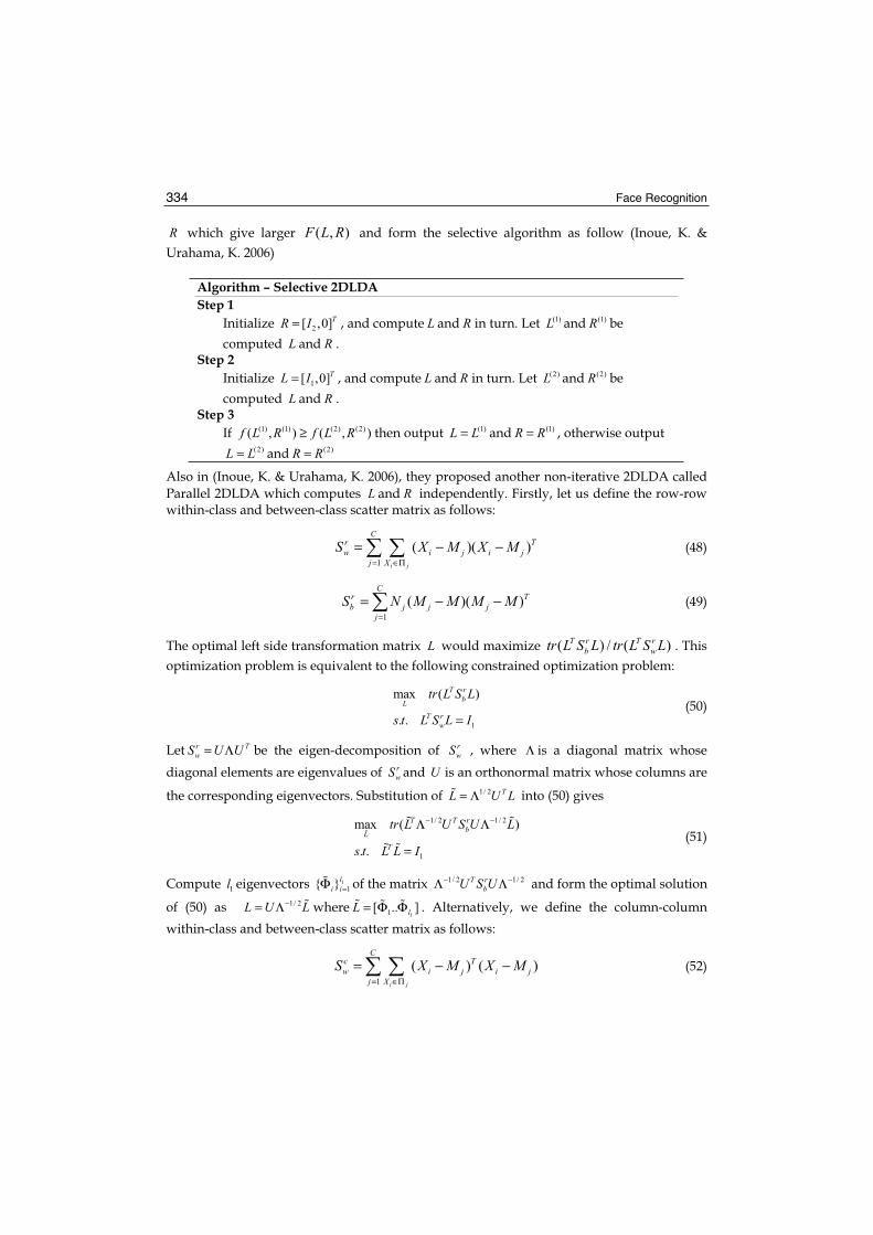
Face Recognition 334
R which give larger ( , )F L R and form the selective algorithm as follow (Inoue, K. & Urahama, K. 2006)
Algorithm – Selective 2DLDA Step 1
Initialize 2[ ,0]TR I= , and compute L and R in turn. Let (1)L and (1)R becomputed L and R .
Step 2Initialize 1[ ,0]TL I= , and compute L and R in turn. Let (2)L and (2)R becomputed L and R .
Step 3If (1) (1) (2) (2)( , ) ( , )f L R f L R≥ then output (1)L L= and (1)R R= , otherwise output
(2)L L= and (2)R R=
Also in (Inoue, K. & Urahama, K. 2006), they proposed another non-iterative 2DLDA called Parallel 2DLDA which computes L and R independently. Firstly, let us define the row-row within-class and between-class scatter matrix as follows:
1
( )( )i j
Cr Tw i j i j
j XS X M X M
= ∈Π
= − − (48)
1
( )( )C
r Tb j j j
jS N M M M M
=
= − − (49)
The optimal left side transformation matrix L would maximize ( ) / ( )T r T rb wtr L S L tr L S L . This
optimization problem is equivalent to the following constrained optimization problem:
1
max ( )
. .
T rbL
T rw
tr L S L
s t L S L I= (50)
Let r TwS U U= Λ be the eigen-decomposition of r
wS , where Λ is a diagonal matrix whose diagonal elements are eigenvalues of r
wS and U is an orthonormal matrix whose columns are
the corresponding eigenvectors. Substitution of 1/ 2 TL U L= Λ into (50) gives
1/ 2 1/ 2
1
max ( )
. .
T T rbL
T
tr L U S U L
s t L L I
− −Λ Λ
= (51)
Compute 1l eigenvectors 1
1{ }li i=Φ of the matrix 1/ 2 1/ 2T rbU S U− −Λ Λ and form the optimal solution
of (50) as 1/ 2L U L−= Λ where11[ .. ]lL = Φ Φ . Alternatively, we define the column-column
within-class and between-class scatter matrix as follows:
1
( ) ( )i j
Cc Tw i j i j
j XS X M X M
= ∈Π
= − − (52)

Image-based Subspace Analysis for Face Recognition 335
1
( ) ( )C
c Tb j j j
jS N M M M M
=
= − − (53)
The optimal left side transformation matrix R would maximize ( ) / ( )T c T cb wtr R S R tr R S R .
This optimization problem is equivalent to the following constrained optimization problem:
2
max ( )
. .
T cbR
T cw
tr R S R
s t R S R I= (54)
Let c TwS V V= Λ be the eigen-decomposition of c
wS , where Λ is a diagonal matrix whose diagonal elements are eigenvalues of c
wS and V is an orthonormal matrix whose columns are
the corresponding eigenvectors. Substitution of 1/ 2 TR V R= Λ into (54) gives
1/ 2 1/ 2
2
max ( )
. .
T T cbR
T
tr R V S V R
s t R R I
− −Λ Λ
= (55)
Compute 2l eigenvectors 2
1{ }li i=Ψ of the matrix 1/ 2 1/ 2T cbV S V− −Λ Λ and form the optimal solution
of (54) as 1/ 2R V R−= Λ where21[ .. ]lR = Ψ Ψ . The parallel 2DLDA can be described as follow
Algorithm – Parallel 2DLDA Step A1
Compute rwS and r
bSStep A2
Compute eigen-decomposition r TwS U U= Λ
Step A3 Compute the first 1l eigenvectors 1
1{ }li i=Φ of the matrix 1/ 2 1/ 2T rbU S U− −Λ Λ and
compute 1/ 2L U L−= Λ where11[ .. ]lL = Φ Φ
Step B1Compute c
wS and cbS
Step B2 Compute eigen-decomposition c T
wS V V= ΛStep B3
Compute the first 2l eigenvectors 2
1{ }li i=Ψ of the matrix 1/ 2 1/ 2T cbV S V− −Λ Λ and
compute 1/ 2R V R−= Λ where21[ .. ]lR = Ψ Ψ
Since the algorithm computes L and R independently, we can interchange Step A1,A2,A3,A4 and Step B1,B2,B3,B4.
5. Conclusions
In this chapter, we have shown the class of low-rank approximation algorithms based directly on image data. In general, those algorithms are reduced to a couple of eigenvalue

Face Recognition 336
problems of row-row and column-column covariance matrices. In contrast to those 1D approaches, the size of the image covariance matrix using image-based approaches is much smaller. As a result, it is easier to evaluate the covariance matrix accurately and less time is required to determine the corresponding eigenvectors. Some future work should be considered such as the relationship between 1D approaches and 2D approaches and an extension of those 2D approaches to higher tensors.
6. References
Belhumeur, P.N.; Hespanha, J.P. & Kriegman, D.J. (1997). Eigenfaces vs. Fisherfaces: recognition using class specific linear projection. Pattern Analysis and Machine Intelligence, IEEE Transactions on, Vol. 19, Issue 7, July 1997, pp. 711 - 720, ISSN 0162-8828
Chris Ding & Jieping Ye (2005). Two-dimensional Singular Value Decomposition (2DSVD) for 2D Maps and Images. Proc. SIAM Int'l Conf. Data Mining (SDM'05), pp. 32-43
D. Xu; S. Yan; L. Zhang; H. Zhang; Z. Liu & H. Shum (2005). Concurrent Subspace Analysis. IEEE Int. Conf. on Computer Vision and Pattern Recognition (CVPR), 2005
Inoue, K. & Urahama, K. (2006). Non-Iterative Two-Dimensional Linear Discriminant Analysis. Pattern Recognition, 2006. ICPR 2006. 18th International Conference on. Vol. 2, pp. 540- 543
Jian Yang; Zhang, D.; Frangi, A.F. & Jing-yu Yang (2004). Two-dimensional PCA: a new approach to appearance-based face representation and recognition. Pattern Analysis and Machine Intelligence, IEEE Transactions on, Vol. 26, Issue 1, Jan 2004, pp. 131- 137, ISSN 0162-8828
Jieping Ye (2004). Generalized low rank approximations of matrices. Proceedings of the twenty-first international conference on Machine learning, pp. 112, ISSN 1-58113-828-5
Jieping Ye; Ravi Janardan & Qi Li (2004). Two-Dimensional Linear Discriminant Analysis. Neural Information Processing Systems 2004
Jun Liu & Songcan Chen (2006). Non-iterative generalized low rank approximation of matrices. Pattern recognition letters, Vol. 27, No. 9, 2006, pp 1002-1008
M. Turk & A. Pentland (1991). Face recognition using eigenfaces. Proc. IEEE Conference on Computer Vision and Pattern Recognition, pp 586–591
Ming Li & Baozong Yuan (2004). A novel statistical linear discriminant analysis for image matrix: two-dimensional Fisherfaces. Signal Processing, 2004. Proceedings. ICSP '04. 2004 7th International Conference on
Songcan Chen; Yulian Zhu; Daoqiang Zhang; Yang Jing-Yu (2005). Feature extraction approaches based on matrix pattern : MatPCA and MatFLDA. Pattern recognition letters, Vol. 26, No. 8, 2005, pp. 1157-1167
Zhizheng Liang; David Zhang & Pengfei Shi (2007). The theoretical analysis of GLRAM and its applications. Pattern recognition, Vol. 40, Issue 3, 2007, pp 1032-1041
18
Nearest Feature Rules and Dissimilarity Representations for Face Recognition Problems
Mauricio Orozco-Alzate and Germán Castellanos-Domínguez Universidad Nacional de Colombia Sede Manizales
Colombia
1. Introduction
Over the last decade, face recognition has been a widely-studied area of research. It has been mainly motivated by a high and always increasing demand of reliable authentication and security systems, as well as by numerous medical-related and human-computer interaction applications; such as posture/gesture recognizers, intelligent multimodal systems and speech therapy software. In addition, a variety of dimensionality reduction techniques and classification rules have been treated. In particular, linear transformations for extracting non-facial or non-geometric features and non-parametric pattern classifiers have been widely employed in the so-called pixel-based approach, which consists in operating directly on the acquired image, without deriving facial features such as the distance between eyes or the area of the mouth. Face recognition is a particular problem of multi-class classification. In general, we are given a set of training objects { }NiX M
iii ,,1,|,),(: =∈= Rxx ω , each of them (pixels from a face image in our particular case) consisting of a M dimensional pattern xi and its label ∈ωi .In pixel-based face recognition problems, feature extraction and feature selection methods are applied in order to reduce the dimensionality. Such methods usually consist in a transformation ZX: →φ , such that )(: xz φ= .The eigenface representation is the simplest and widest used dimensionality reduction technique employed in pixel-based face recognition. It consists in the principal component analysis (PCA) or the Karhunen-Loève transform (KL), differing mainly at the structure of the covariance matrix. Let x be a vector formed by all the rows of an image, the prototype
faces are arranged on a matrix [ ]xx μxμxX −−= N1 , where [ ]=
==N
1n nN1E xxμx . Due to
the fact that the number of training faces N is often smaller than the face dimension d, it is more advisable to calculate the eigenvectors of the N×N covariance matrix XXX
T' = ,
instead of those of the d×d covariance matrix TXXX = . The eigenvectors wi corresponding to the p largest eigenvalues are called eigenfaces and determine a transformation matrix [ ]
pN21eigen wwwW = , where NNp ≤ is the number of principal components to be
considered in further procedures. A specific value for Np is selected according to some

Face Recognition 338
criterion, e.g. the information percentage on the eigenvalues. A feature point is transformed by
( )xμxWz −= Teigen (1)
This chapter is concerned with four subjects. The first one is a conceptual and experimental review of the nearest feature classifiers; some bibliographical remarks as well as theoretical and empirical conclusions are given. The second subject is a quantification of the computational complexity of the nearest feature rules, by using an economic model which takes into account a trade-off between classifier error and evaluation complexity. Complexities of these classifiers are estimated in terms of orders (big-oh notation) and measured in FLOPs. The study includes error-complexity curves and complexity costs, resembling a cost-benefit analysis. The third one corresponds to a face recognition task based on dissimilarity representations, which shows that normal density-based (Bayesian) classifiers constructed on such representations are an alternative approach to the direct application of the nearest neighbor rule. The last subject is aimed to present a conceptual discussion on the relationship between the nearest feature rules and dissimilarity representations, particularly the so-called generalized dissimilarity representations and their potential application to face recognition problems as well as to other applications. Some open and apparently promising issues to be considered for further research are also discussed in the concluding section.
2. The nearest feature classifiers
In classification theory, there is an approach completely independent of statistical knowledge or assumptions, the so-called distribution free classification, often referred to as nonparametric techniques. Such an approach includes classification algorithms which can be described without reference to probability distributions; i.e. without the assumption that the forms of the underlying densities are known (Duda et al., 2000). Nonparametric procedures can be roughly divided into two branches: firstly, methods for estimating the underlying density functions, including the Parzen-window method and the kn-nearest neighbor estimation; secondly, procedures for estimating directly the a posteriori probabilities such as the well-known k-nearest neighbor rule (k-NN) which, in spite of its simplicity, has been successfully used in a considerable variety of applications. Nonetheless, it requires a significant amount of storage and computational effort; such a problem can be partly solved by using the condensed nearest neighbor rule (CNN) (Hart, 1968). In addition, the k-NN classifier suffers of a potential loss of accuracy when a small set of prototypes is available. To overcome this shortcoming, the nearest feature classifiers were developed. They are also a type of nonparametric techniques, which are based on a measure of distance between the query point and the prototypes or a function calculated from them, such as a line, a plane or a space. In this work, we consider four different nearest feature rules: k-nearest-neighbor or k-NN, k-nearest-feature-line or k-NFL, k-nearest-feature-plane or k-NFP and nearest-feature-space or NFS. The two last ones were proposed in (Chien & Wu, 2002) as a complete geometric generalization of k-NFL. Before defining the nearest feature classifiers, a brief comment on notation is given. Consider a collection of training faces { }c
Niii nC,,1i,|,),(:Z ⋅=∈ω= Rzz , where C
denotes the number of classes and nc the number of objects per class. We assume, without

Nearest Feature Rules and Dissimilarity Representations for Face Recognition Problems 339
loss of generality, a transformed point z because a dimensionality reduction technique is usually applied before using a classifier; however, for the sake of notation simplicity, x and zwill be used indistinctly to denote a pattern. The nearest feature rules are defined as follows.
2.1 The k-Nearest-Neighbor Rule
The simplest nonparametric method for classification should be considered k-NN (Cover & Hart, 1967). This rule classifies z by assigning it the class label most frequently represented among the k nearest prototypes; i.e., by finding the k neighbors with the minimum distances between z and all prototype feature points {zci,1 c C,1 i nc}. For k=1, the rule can be written as follows:
( ) ( ),,dmin,d cini1C;c1icc
zzzz≤≤≤≤
= (2)
where d(z,zci)= z-zci is usually the Euclidean norm. In this case, the number of distance
calculations is =
=C
1c cnn .
2.2 The k-Nearest-Feature-Line
The k-nearest-feature-line rule, or k-NFL (Li & Lu, 1999), is an extension of the k-NN classifier. This method generalizes each pair of prototype feature points belonging to the same class, {zci,zcj} by a linear function c
ijL , which is called the feature line (see Figure 1). The line is
expressed by the span ( )cjcicij ,spL zz= . The query z is projected onto c
ijL as a point cijp . This
projection is computed as
),,( cicjcicij zzzzp −τ+= (3)
where τ=(z-zci)(z-zci)/ zcj-zci 2, which is called the position parameter. The classification of zis done by assigning it the class label most frequently represented among the k nearest feature lines, for k=1 that means:
( ) ( ),L,dminL,d cijji;nji,1C;c1
cji
c
zz≠≤≤≤≤
= (4)
where ( ) cij
cijL,d pzz −= . In this case, the number of distance calculations is
=−=
C
1c ccL 2/)1n(nn .
Figure 1. Feature line and projection point onto it

Face Recognition 340
2.3 The k-Nearest-Feature-Plane
The k-nearest-feature-plane rule, or k-NFP, is an extension of the k-NFL classifier. This classifier assumes that at least three linearly independent prototype points are available for each class. It generalizes three feature points {zci,zcj,zcm} of the same class by a feature plane
cijmF (see Figure 2); which is expressed by the span ( )cmcjci
cijm ,,spF zzz= . The query z is
projected onto cijmF as a point c
ijmp . The projection point can be calculated as follows:
,Tcijm
1cijm
Tcijm
cijm
cijm zZZZZp
−=
(5)
where [ ]cmcjcicijm zzzZ = . Considering k=1, the query point z is classified by assigning it the
class label , according to
( ) ( ),F,dminF,d cijmmji;nmj,i,1C;c1
cmji
c
zz≠≠≤≤≤≤
= (6)
where ( ) cijm
cijmF,d pzz −= . In this case, the number of distance calculations is
=−−=
C
1c cccF 6/)2n)(1n(nn .
Figure 2. Feature plane and projection point onto it
2.4 The Nearest-Feature-Space Rule
The nearest-feature-space rule, or NFS, extends the geometrical concept of k-NFP classifier. It generalizes the independent prototypes belonging to the same class by a feature space
( )ccn2c1c
c ,,,spS zzz= . The query point z is projected onto the C spaces as follows:
,Tc1
cTccc zZZZZp−
= (7)
where [ ]ccn2c1c
c zzzZ = . The query point z is classified by assigning it the class label ,according to
( ) ( ) c
Cc1
c
Cc1
c minS,dminS,d pzzz −==≤≤≤≤
(8)
The number of distance calculations is always equals to C.

Nearest Feature Rules and Dissimilarity Representations for Face Recognition Problems 341
2.5 Theoretical geometric differences
It was geometrically shown in (Chien & Wu, 2002) that the distance of z to cijmF is smaller
than that to the feature line. Moreover, the distance to the feature line is nearer compared with the distance to two prototype feature points. This relation can be written as follows:
( ) ( ) ( ) ( )( ) ( ) ( ) ( )( )cmcjcicmi
cjm
cij
cijm ,d,,d,,dminL,d,L,d,L,dminF,d zzzzzzzzzz ≤≤ (9)
In addition,
( ) ( )cijmCc1
c F,dminS,d zz≤≤
= (10)
In consequence, k-NFL classifier is supposed to capture more variations than k-NN, k-NFP should handle more variations of each class than k-NFL and NFS should capture more variations than k-NFP. So, it is expected that k-NFL performs better than k-NN, k-NFP is more accurate than k-NFL and NFS outperforms k-NFP.
2.6 Asymptotic behavior of the nearest feature rules
The problem of determining the error bound for the nearest feature rules can be addressed following the procedure to derive the error rate for the nearest neighbor rule; i.e. k-NN for k=1. The nearest feature rules are sub-optimal procedures as the k-NN rule; that is, they lead to an error rate greater than the minimum possible, the Bayes rate (Duda et al., 2000). In particular, for the k-NN rule with an unlimited number of prototypes, the error rate is never worse than twice the Bayes rate. In this sense, the infinite-sample conditional average probability of error P(e|x) and the unconditional average probability of error P(e) are analyzed to find their minimum possible values: P*(e|x) and P*(e) respectively. Values of P(e|x) and P(e) are related, through the density p(x), by
.dx)x(p)x|e(P)e(P = (11)
Let us define the m-th state of nature ωm(x) by )x|(Pmax)x|(P iim ω=ω . The probability of
error is minimized by the Bayes’ decision rule, minimizing P(e|x) for every x, thus
)x|(P1)x|e(*P mω−= , (12)
and
= dx)x(p)x|e(*P*P . (13)
Expression (13) is called the Bayes rate.A conditional probability of error P(e|x,x’) must be defined because the nearest neighbor rule depends on the samples, particularly on both the nearest prototype x’ to a test point x and on the point x itself. P(e|x) is obtained by averaging over x’
= 'dx)x|'x(p)'x,x|e(P)x|e(P . (14)

Face Recognition 342
In order to simplify the analysis of (14), the infinite-sample case, i. e. when n goes to infinity, is considered. In those conditions, the conditional density p(x’|x) approaches to a delta function centered at x:p(x’|x)→δ(x’-x) (See also (Duda et al., 2000) for a detailed demonstration). Now, an expression for P(e|x,x’) is derived as follows: Let (x1,θ1),(x2,θ2),…,(xn,θn) be n independently drawn labelled samples, where
{ }c1j ,, ωω∈θ for j=1,…,n. Suppose that a test point (x,θ) and its nearest training sample (xj’,θj’) are selected. Since the states of nature, when x and xj’ were drawn, are independent, we have
)'x|'(P)x|(P)'x,x|',(P jjjj θθ=θθ ; (15)
according to the nearest neighbor rule, an error is made if θ≠θj and, consequently, the conditional probability of error Pn(e|x,xj’) is given by
.)'x|(P)x|(P1
)'x,x|',(P1)'x,x|e(P
c
1ijii
c
1ijiijn
=
=
ωω−=
ω=θω=θ−= (16)
Substituting (16) in (14):
=
=∞→
ω−=
−δωω−=
c
1ii
2
c
1iiinn
)x|(P1
'dx)x'x()'x|(P)x|(P1)x|e(Plim (17)
In addition, if )e(PlimP nn ∞→= and using (11) and (17) we have
ω−=
=
=
=
=
∞→
∞→
∞→
dx)x(p)x|(P1
dx)x(p)x|e(Plim
dx)x(p)x|e(Plim
)e(PlimP
c
1ii
2
nn
nn
nn
(18)
Comparing (13) and (18), it can easily be seen that P* is a lower bound on P. In order to
calculate an upper bound, expression =
ωc
1i i2 )x|(P in (18) is examined to determine how it
is minimized. Such an expression can be rewritten as
= ≠
ω+ω=ωc
1i mii
2m
2i
2 )x|(P)x|(P)x|(P , (19)

Nearest Feature Rules and Dissimilarity Representations for Face Recognition Problems 343
and the bound for =
ωc
1i i2 )x|(P is found by minimizing the term
≠ω
mi i2 )x|(P , s.t.:
0)x|(P i ≥ω (20)
≠
=ω−=ωmi
mi )x|e(*P)x|(P1)x|(P (21)
=ω
c
1i i2 )x|(P is minimized if mj,i),x|(P)x|(P ji ≠∀ω=ω . Besides, from (21) we have:
=−
≠−=ω
mi)x|e(*P1
mi1c
)x|e(*P)x|(P i (22)
The following inequalities can be derived from the expressions above:
= −+−≥ω
c
1i
22
i2
1c)x|e(*P))x|e(*P1()x|(P (23)
and
= −−≤ω−
c
1ii
2 )x|e(*P1c
c)x|e(*P2)x|(P1 (24)
By substituting (24) in (18), it can be seen that P 2P*. Furthermore, a tight expression can be obtained by observing the variance of P*(e|x) (Duda et al., 2000):
[ ] [ ]0*Pdx)x(p)x|e(*P
dx)x(p*P)x|e(*Px|)e(*Pvar
22
2
≥−=
−=(25)
and, in consequence,
≥ 22 *Pdx)x(p)x|e(*P (26)
Using (24) and (26) in (18), we obtain the inequality:
−−≤≤ *P
1cc2*PP*P , (27)
which shows that the nearest neighbour error rate P in a multi-class (c classes) problem, having an infinite collection of training data, is always less than or equal to twice the Bayes rate. An elegant conclusion from (27) is given in (Duda et al., 2000): “at least half of the classification information in an infinite data set resides in the nearest neighbor”. Having an arbitrarily large number of prototypes, training or representation sets are fully informative and representative of the underlying processes. Since the nearest feature rules

Face Recognition 344
attempt to enrich the representation and, under the condition cited above, available prototypes are fully representative, we intuitively do not expect a difference between the asymptotic behavior of the k-NN rule and the asymptotic behavior of the nearest feature classifiers for the infinite-sample case. The finite-sample case cannot be addressed by using such a simple reasoning. In fact, questions such as how rapidly the performance converges to the asymptotic value have still not been solved for the k-NN rule (Duda et al., 2000).
3. Quantifying the Computational Complexity of the Nearest Feature Classifiers
This section is devoted to quantifying the computational complexity of the nearest feature classifiers, by using an economic model which takes into account a trade-off between classifier error and evaluation complexity. The model is applied to the face recognition problem, which is the framework where these classifiers were originally proposed. Classifiers are also studied by measuring them in orders, denoted by the Landau symbol O (big-oh notation).
3.1 Complexity of the Nearest Feature Classifiers
Due to, as mentioned above, the nearest feature classifiers are non-parametric, the number of samples in the training set (prototypes) has a strong influence on the evaluation complexity. Since in modern computer systems, additions and multiplications are comparable in complexity (de Ridder et al., 2002), we can consider that: • sum of two d-dimensional vectors costs d additions, therefore it has a complexity of d, • multiplication of two d-dimensional vectors costs d additions and d multiplications, so
it has a complexity of 2d, • a scalar-vector multiplication has a complexity of d, • multiplying a m×d matrix by a d×1 vector has a complexity of 2dm, • multiplying a m×d matrix by a d×m matrix has a complexity of m2(2d-1),• a m×m matrix inversion has a complexity of O(m3).Considering that Euclidean distance d(z1,z2) is used in all of them, whose complexity is 3d if z1 and z2 are d-dimensional, then we have: 1. k-NN: distances to all prototypes have to be calculated (2nd) and the minimum will
have to be stored in a sorted list of k nearest prototypes (n⋅log2k). The total complexity therefore is n(3d+log2k).
2. k-NFL: projection points onto lines (Eq. (3)) have to be calculated (14dnL) and also distances to all feature lines (2dnL). The minimum will have to be stored in a sorted list of k nearest prototypes (nL⋅log2k). In consequence, the total complexity is nL(16d+log2k).
3. k-NFP: projection points on planes (Eq. (5)) have to be calculated (nFO(30d+36)) and also distances to all feature planes (2dnF). The minimum will have to be stored in a sorted list of k nearest prototypes (nF⋅log2k). The total complexity therefore is nF(2d+log2k+O(30d+36)).
4. NFS: projection points on spaces (Eq. (7)) have to be calculated ( )( )( )3
c2cc n1d2ndn4C +++ and also distances to all feature spaces (2dC) and the
minimum will have to be found (C⋅log2C). Consequently, the total complexity is ( )( )Clogd2n1d2ndn4C 2
3c
2cc +++++ .

Nearest Feature Rules and Dissimilarity Representations for Face Recognition Problems 345
3.2 Error-Complexity Curves
Complexity can be empirically studied by exploring the error-complexity trade-off. As in a cost-benefit analysis, a series of experiments should be conducted, varying the number of prototypes in order to investigate the dependency of the performance on it. For feature extraction, the eigenface representation was applied (cf. Section 1). Obviously, computational complexity can be lowered by retaining as fewer eigenfaces as possible; nonetheless, 40 eigenfaces are sufficient for a very good description of the training set (Chin & Suter, 2004). We have used k=1 for all the classifiers; nonetheless, k could be optimized by the leave-one-out procedure. Data sets used here as examples are: • The AT&T (previously ORL) Database of Faces, with C=40, d=93×112 pixels which was
reduced up to d=40 and { }.5,4,3Cn ⋅∈• The Sheffield (previously UMIST) Face Database, with C=20, d=93×112 pixels which
was reduced up to d=40 and { }.9,7,5,3Cn ⋅∈Error e (in %, measured on an independent set of 5 examples per class) vs. computational complexity f (in FLOPs) for the AT&T database of faces is shown in Figure 3. Similarly, the error e (in %, measured on an independent set of 9 examples per class) vs. computational complexity f (in FLOPs) for the Sheffield Face Database is shown in Figure 4. In both cases the number of FLOPs corresponds to the classification of a single example z.
Figure 3. Classifier complexity f (in FLOPs) vs. e (in %) for the AT&T database of faces
When NFS is applied for three prototypes per class, it becomes k-NFP. It is noteworthy that performance could decline. In practice, k-NFP classifier is not advisable because its computational complexity becomes too high. If a sufficient number of prototypes is available, for example 5 or 9 prototypes per class for each database, the best choice would be k-NFL. Only in those cases where the number of prototypes is not large enough to cover variations for each object, the more expensive nearest feature classifiers should be used.
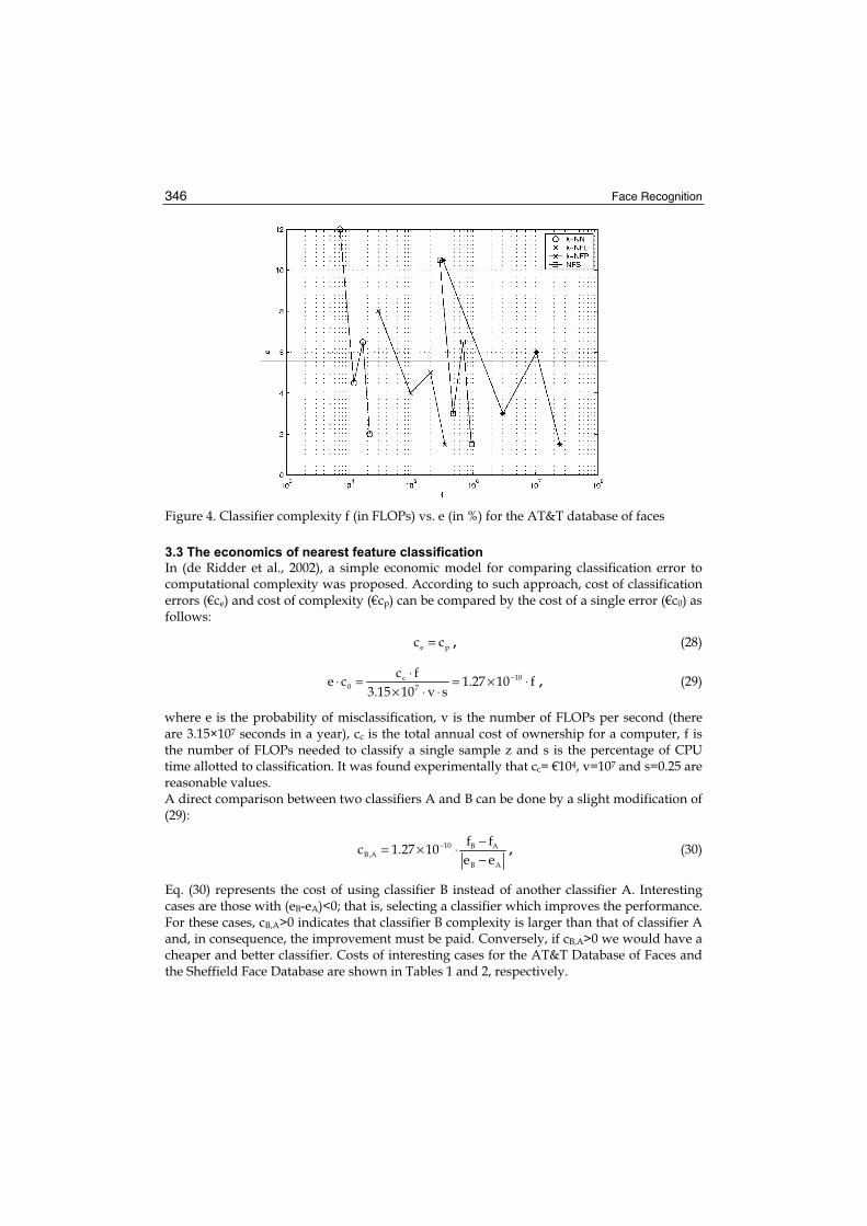
Face Recognition 346
Figure 4. Classifier complexity f (in FLOPs) vs. e (in %) for the AT&T database of faces
3.3 The economics of nearest feature classification
In (de Ridder et al., 2002), a simple economic model for comparing classification error to computational complexity was proposed. According to such approach, cost of classification errors (€ce) and cost of complexity (€cp) can be compared by the cost of a single error (€c0) as follows:
pe cc = , (28)
f1027.1sv1015.3
fcce 107
c0 ⋅×=
⋅⋅×⋅
=⋅ − , (29)
where e is the probability of misclassification, v is the number of FLOPs per second (there are 3.15×10⁷ seconds in a year), cc is the total annual cost of ownership for a computer, f is the number of FLOPs needed to classify a single sample z and s is the percentage of CPU time allotted to classification. It was found experimentally that cc= €104, v=107 and s=0.25 are reasonable values. A direct comparison between two classifiers A and B can be done by a slight modification of (29):
AB
AB10A,B ee
ff1027.1c−−⋅×= − , (30)
Eq. (30) represents the cost of using classifier B instead of another classifier A. Interesting cases are those with (eB-eA)<0; that is, selecting a classifier which improves the performance. For these cases, cB,A>0 indicates that classifier B complexity is larger than that of classifier A and, in consequence, the improvement must be paid. Conversely, if cB,A>0 we would have a cheaper and better classifier. Costs of interesting cases for the AT&T Database of Faces and the Sheffield Face Database are shown in Tables 1 and 2, respectively.

Nearest Feature Rules and Dissimilarity Representations for Face Recognition Problems 347
AClassifier k-NN k-NFL k-NFP NFS
B 3 prototypes per class k-NN — — — — k-NFL 0.0002 — — — k-NFP 0.0027 0.0068 — * NFS 0.0018 0.0044 * —
4 prototypes per class k-NN — — — — k-NFL 0.0007 — — — k-NFP 0.0143 0.0690 — * NFS 0.0037 0.0161 * —
5 prototypes per class k-NN — — — — k-NFL 0.0015 — * -0.0190 k-NFP 0.0558 * — 0.1438 NFS 0.0117 — — —
*: eB=eA; —: (eB - eA) > 0
Table 1. Economics of nearest feature classifiers. AT&T database of faces
AClassifier k-NN k-NFL k-NFP NFS
B 3 prototypes per class k-NN — — — — k-NFL 0.0001 — -0.0015 -0.0013 k-NFP 0.0027 — — * NFS 0.0024 — * —
5 prototypes per class k-NN — — — — k-NFL 0.0022 — — — k-NFP 0.0253 0.0368 — * NFS 0.0039 0.0048 * —
7 prototypes per class k-NN — — — * k-NFL 0.0016 — -0.1287 -0.0041 k-NFP 0.2623 — — 0.2452 NFS * — — —
9 prototypes per class k-NN — — — — k-NFL 0.0084 — * * k-NFP 0.6261 * — * NFS 0.0233 * * —
*: eB=eA; —: (eB - eA) > 0 Table 2. Economics of nearest feature classifiers. Sheffield face database
Face Recognition 348
k-NFP classifier is always the most expensive option. The cheaper solution which gives an acceptable error in comparison with the best possible performance is k-NFL; in fact, in several cases using k-NFL instead of other nearest feature classifier is a saving on the cost of error-complexity. In general, costs of preferring NFS are acceptable.
4. Dissimilarity-based face recognition
The concept of proximity is essential in learning processes. Identifying differences or, conversely, detecting shared commonalities are typically carried out by using a suitable proximity measure, often referred to as a dissimilarity. Such a proximity can be modelled in different ways, according to the nature of data; e.g. as a classical distance between vector representations or by using edit distances between structural descriptions, such as shapes or sequences. A wide-scope approach, the dissimilarity representation for pattern recognition (P kalska & Duin, 2005a), was proposed on the basis of such proximity measures. Statistical and structural learning techniques can be directly used with dissimilarity representations, naturally fitting for a variety of applications, e.g. face recognition problems. In addition, since dissimilarity measures are considered very general, they are not constrained to Euclidean or metric behaviors, neither to positive semidefinite structures as it is imposed beforehand in kernel methods. The aim of this Section is to review the practical foundations of the dissimilarity-based approach and to explore its application for a simple face recognition problem.
4.1 Dissimilarity representations
A dissimilarity representation of objects is based on their pairwise comparisons. Consider a representation set R:={p1,p2,…,pn} and a dissimilarity measure d. An object x is represented as a vector of the dissimilarities computed between x and the prototypes from R, i.e. D(x,R)=[d(x,p1),d(x,p2),…,d(x,pn)]. For a set T of N objects, it extends to an N×n dissimilarity matrix (P kalska et al., 2006):
( ) =
Nn3N2N1N
n3333231
n2232221
n1131211
N
3
2
1
n321
dddd
dddddddddddd
x
xxx
R,TD
pppp
(31)
where djk=D(xj,pk).For dissimilarities, the geometry is contained in the definition, giving the possibility to include physical background knowledge; in contrast, feature-based representations usually suppose a Euclidean geometry. Important properties of dissimilarity matrices, such as metric nature, tests for Euclidean behavior, transformations and corrections of non-Euclidean dissimilarities and embeddings, are discussed in (P kalska & Duin, 2005b). When the entire T is used as R, the dissimilarity representation is expressed as an N×Ndissimilarity matrix D(T,T). Nonetheless, R may be properly chosen by prototype selection procedures (P kalska et al., 2006).

Nearest Feature Rules and Dissimilarity Representations for Face Recognition Problems 349
4.2 Classifiers in dissimilarity spaces
Building a classifier in a dissimilarity space consists in applying a traditional classification rule, considering dissimilarities as features; that is, in practice, a dissimilarity-based classification problem is addressed as a traditional feature-based one. Even though the nearest neighbor rule is the reference method to discriminate between objects represented by dissimilarities, it suffers from a number of limitations. Previous studies (P kalska et al., 2001; P kalska & Duin, 2002; Paclík & Duin, 2003; P kalska et al., 2004; Orozco-Alzate et al., 2006) have shown that Bayesian (normal density based) classifiers, particularly the linear (LDC) and quadratic (QDC) normal based classifiers, perform well in dissimilarity spaces and, sometimes, offer a more accurate solution. For a 2-class problem, the LDC based on the representation set R is given by
( )( ) ( ) ( ) ( ))2(
)1()2()1(
1T
)2()1( PP
logC21R,xDRx,Df +−×+−= − mmmm (32)
and the QDC is derived as
( )( ) ( ) ( )( ) ( )=
− ++−×−−=2
1i 2
)1(
)2(
)1()i(
1)i(
T)i(
i
C
Clog
pp
log2)R,x(DCR,xD1Rx,Df mm (33)
where C is the sample covariance matrix, C(1) and C(2) are the estimated class covariance matrices, and m(1) and m(2) are the mean vectors, computed in the dissimilarity space D(T,R). P(1) and P(2) are the class prior probabilities. If C is singular, a regularized version must be used. In practice, the following regularization is suggested for λ=0.01 (P kalska et al., 2006):
( ) ( )CdiagC1Creg λ+λ−=λ (34)
Nonetheless, regularization parameter should be optimized in order to obtain the best possible results for the normal density based classifiers. Other classifiers can be used in dissimilarity spaces, usually by a straightforward implementation. Nearest mean linear classifiers, Fisher linear discriminants, support vector machines (SVMs), among others are particularly interesting for being used in generalized dissimilarity spaces. In addition, traditional as well as specially derived clustering techniques can be implemented for dissimilarity representations, see (P kalska & Duin, 2005c) for a detailed discussion.
4.3 Experimental results
As in Section 3.2, experiments were conducted on the AT&T and the Sheffield datasets, using 40 eigenfaces for an initial representation. Dissimilarity representations were constructed by calculating pairwise Euclidean distances on the eigenface representations. In order to compare different classifiers, the k-NN rule and the LDC and QDC classifiers built on the dissimilarity representations were used. Experiments were performed 25 times for randomly chosen training and test sets. Since in this study we are particularly interested in recognition accuracy rather than in computational complexity and storage requirements, the entire training set T has been used as the representation set R. Nonetheless, R may be properly reduced by prototype selection procedures (P kalska et al., 2006). Training and testing sets were generated by selecting equal partitions for the classes.

Face Recognition 350
Figures 5 and 6 present the results, in terms of classification errors as a function of the number of training objects randomly chosen. Figure 5 presents the results for the AT&T database; similarly, the results for the Sheffield dataset are shown in Figure 6. Standard deviations for averaged test error decrease rapidly, varying around 0.15 and 0.08 after at least 6 training objects per class are available; for clarity reasons, standard deviations are not given.
Figure 5. Average classification error as a function of the number of prototypes per class for the ORL database of faces
Figure 6. Average classification error as a function of the number of prototypes per class for the Sheffield database of faces
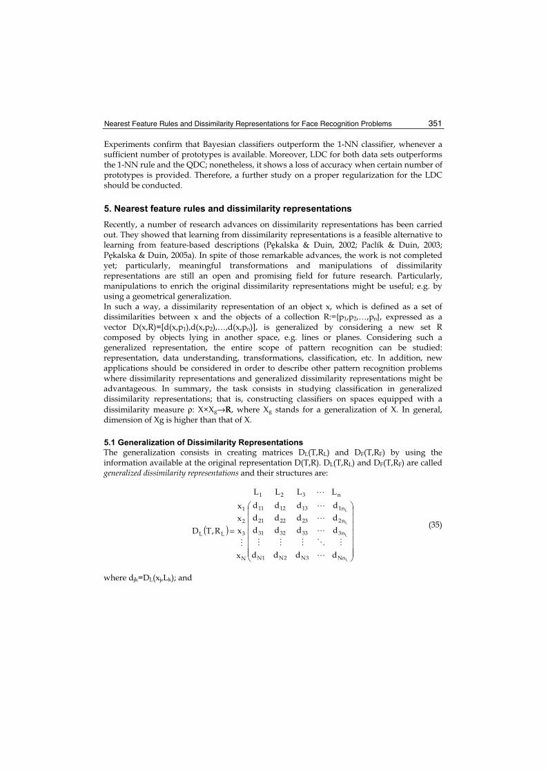
Nearest Feature Rules and Dissimilarity Representations for Face Recognition Problems 351
Experiments confirm that Bayesian classifiers outperform the 1-NN classifier, whenever a sufficient number of prototypes is available. Moreover, LDC for both data sets outperforms the 1-NN rule and the QDC; nonetheless, it shows a loss of accuracy when certain number of prototypes is provided. Therefore, a further study on a proper regularization for the LDC should be conducted.
5. Nearest feature rules and dissimilarity representations
Recently, a number of research advances on dissimilarity representations has been carried out. They showed that learning from dissimilarity representations is a feasible alternative to learning from feature-based descriptions (P kalska & Duin, 2002; Paclík & Duin, 2003; P kalska & Duin, 2005a). In spite of those remarkable advances, the work is not completed yet; particularly, meaningful transformations and manipulations of dissimilarity representations are still an open and promising field for future research. Particularly, manipulations to enrich the original dissimilarity representations might be useful; e.g. by using a geometrical generalization. In such a way, a dissimilarity representation of an object x, which is defined as a set of dissimilarities between x and the objects of a collection R:={p1,p2,…,pn}, expressed as a vector D(x,R)=[d(x,p1),d(x,p2),…,d(x,pn)], is generalized by considering a new set R composed by objects lying in another space, e.g. lines or planes. Considering such a generalized representation, the entire scope of pattern recognition can be studied: representation, data understanding, transformations, classification, etc. In addition, new applications should be considered in order to describe other pattern recognition problems where dissimilarity representations and generalized dissimilarity representations might be advantageous. In summary, the task consists in studying classification in generalized dissimilarity representations; that is, constructing classifiers on spaces equipped with a dissimilarity measure ρ: X×Xg→R, where Xg stands for a generalization of X. In general, dimension of Xg is higher than that of X.
5.1 Generalization of Dissimilarity Representations
The generalization consists in creating matrices DL(T,RL) and DF(T,RF) by using the information available at the original representation D(T,R). DL(T,RL) and DF(T,RF) are called generalized dissimilarity representations and their structures are:
( ) =
L
L
L
L
Nn3N2N1N
n3333231
n2232221
n1131211
N
3
2
1
LL
n321
dddd
dddddddddddd
x
xxx
R,TD
LLLL
(35)
where djk=DL(xj,Lk); and

Face Recognition 352
( ) =
F
F
F
F
Nn3N2N1N
n3333231
n2232221
n1131211
N
3
2
1
FF
n321
dddd
dddddddddddd
x
xxx
R,TD
FFFF
(36)
where djk=DF(xj, Fk).D(T, RL) and D(T, RF) are high dimensional matrices because the original representation set R is generalized by combining all the pairs (RL) and all the triplets (RF) of prototypes of the same class. In consequence, a suitable procedure for feature selection (dimensionality reduction) is needed in order to avoid the curse of the dimensionality. A dissimilarity matrix D(T,R)=(dij) is composed of C×C submatrices as follows:
( ) ,
DDD
DDD
DDD
RT,D
21
22221
11211
=
CCCC
C
C
(37)
where Dii and Dij, i j contain intraclass and interclass distances respectively. All the possible dissimilarities between objects are available but the original feature points are not. Nonetheless, it is possible to compute the distances to feature lines from the dissimilarities. The problem consists in computing the height of a scalene triangle as shown in Figure 7.
Figure 7. Height of a scalene triangle corresponding to the distance to a feature line
Let us define s=(djk+dij+dik)/2. Then, the area of the triangle is given by:
;)ds)(ds)(ds(sA ikijjk −−−= (38)
but we also know that area, assuming dij as base, is:
2hd
A ij= (39)
So, we can solve (38) and (39) for h, which is the distance to the feature line. The generalized dissimilarity representation in (35) is constructed by replacing each entry of D(T,RL) by the
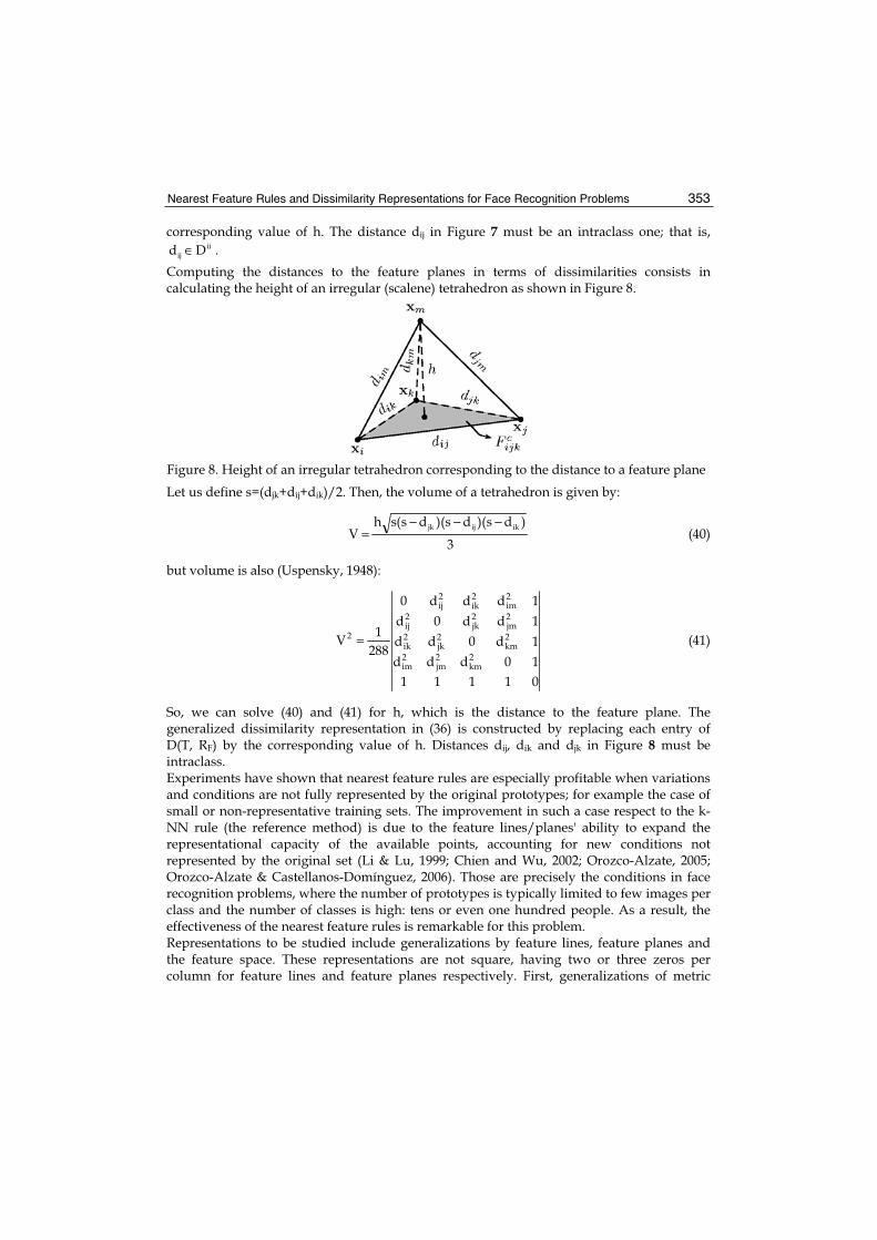
Nearest Feature Rules and Dissimilarity Representations for Face Recognition Problems 353
corresponding value of h. The distance dij in Figure 7 must be an intraclass one; that is, ii
ij Dd ∈ .Computing the distances to the feature planes in terms of dissimilarities consists in calculating the height of an irregular (scalene) tetrahedron as shown in Figure 8.
Figure 8. Height of an irregular tetrahedron corresponding to the distance to a feature plane
Let us define s=(djk+dij+dik)/2. Then, the volume of a tetrahedron is given by:
3
)ds)(ds)(ds(shV ikijjk −−−
= (40)
but volume is also (Uspensky, 1948):
0111110ddd1d0dd1dd0d1ddd0
2881V
2km
2jm
2im
2km
2jk
2ik
2jm
2jk
2ij
2im
2ik
2ij
2 = (41)
So, we can solve (40) and (41) for h, which is the distance to the feature plane. The generalized dissimilarity representation in (36) is constructed by replacing each entry of D(T, RF) by the corresponding value of h. Distances dij, dik and djk in Figure 8 must be intraclass. Experiments have shown that nearest feature rules are especially profitable when variations and conditions are not fully represented by the original prototypes; for example the case of small or non-representative training sets. The improvement in such a case respect to the k-NN rule (the reference method) is due to the feature lines/planes' ability to expand the representational capacity of the available points, accounting for new conditions not represented by the original set (Li & Lu, 1999; Chien and Wu, 2002; Orozco-Alzate, 2005; Orozco-Alzate & Castellanos-Domínguez, 2006). Those are precisely the conditions in face recognition problems, where the number of prototypes is typically limited to few images per class and the number of classes is high: tens or even one hundred people. As a result, the effectiveness of the nearest feature rules is remarkable for this problem. Representations to be studied include generalizations by feature lines, feature planes and the feature space. These representations are not square, having two or three zeros per column for feature lines and feature planes respectively. First, generalizations of metric

Face Recognition 354
representations will be considered because the generalization procedure requires constructing triangles and tetrahedrons and, as a consequence, generalizing non-metric dissimilarity representations might produce complex numbers when solving equations for heights. To construct classifiers based on generalized dissimilarity representations, we should proceed similarly as dissimilarity-based classifiers are built. That is, using a training set T and a representation set R containing prototype examples from T. Prototype lines or planes considered will be selected by some prototype selection procedure; classifiers should be built on D(T,RL) and D(T,RF). Different sizes for the representation set R must be considered. Enriching the dissimilarity representations implies a considerable number of calculations. The number of feature lines and planes grows rapidly as the number of prototypes per class increases; in consequence, computational effort may become high, especially if a generalized representation is computed for an entire set. When applying traditional statistical classifiers to dissimilarity representations, dissimilarities to prototypes may be treated as features. As a result, classifiers built in enriched dissimilarity spaces are also subject to the curse of dimensionality phenomenon. In general, for generalized dissimilarity representations Dg(T,Rg), the number of training objects is small relative to the number of prototype lines or planes.According to the two reasons above, it is important to use dimensionality reduction techniques —feature extraction and feature selection methods— before building classifiers in generalized dissimilarity representations. Systematic approaches for prototype selection such as exhaustive search and the forward selection process lead to an optimal representation set; however, they require a considerable number of calculations. Consequently, due to the increased dimensionality of the enriched representations, the application of a systematic prototype selection method will be computationally expensive. Nonetheless, it has been shown that non-optimal and computationally simple procedures such as Random and RandomC may work well (P kalska et al., 2006).
6. Conclusion
In this chapter, we presented a series of theoretical and experimental considerations regarding the nearest feature rules and dissimilarity representations for face recognition problems, analyzed separately as well as a combined approach. Firstly, a study about the asymptotic behavior of the nearest feature classifiers was conducted, following the well-known procedure derived for the k-NN rule. We concluded that, if an arbitrarily large number of samples is available, there is no significant difference between k-NN and its geometric generalizations: the nearest feature rules. Moreover, as for k-NN, it is not possible to say something general about the asymptotic behavior in the finite-sample case. It might be possible to perform an analysis for specific distributions; perhaps without loss of generality. Consequently, further conceptual considerations and experiments are required. Quantifying the computational complexity of classifiers is very important in the selection of a particular algorithm. Complexity of algorithms is usually measured in terms of orders; nonetheless, such an approach is not precise. An evaluation of the error-complexity trade-off for the nearest feature classifiers has been presented in Section 3. We have also studied the complexity of nearest feature classifiers, in terms of the number of additions and multiplications associated to their evaluation, as well as through error-complexity curves and a comparative study considering error and complexity. It was shown that k-NFP is too

Nearest Feature Rules and Dissimilarity Representations for Face Recognition Problems 355
expensive for practical applications and that k-NFL and NFS are better options to overcome the representational limitations of k-NN. Even though nearest feature rules are well-performing classifiers, their computational complexity is too high. If there is a maximum acceptable response delay for the particular application and a considerable number of prototypes is available, an effective way to overcome this shortcoming might be to use parallel computation. We have explored and tested a dissimilarity-based strategy for face recognition. Two simple classification problems were conducted: the classic ORL database and the Sheffield data set. Dissimilarity representation was derived by applying the eigenface transformation and, afterwards, the Euclidean distance between the eigenface representations. Such a representation allowed us for using traditional statistical decision rules, particularly normal density based classifiers. The 1-NN rule was employed as a reference for performance comparison. Those experiments confirm that Bayesian classifiers outperform the 1-NN classifier, when a sufficient number of prototypes is provided. The LDC constructed for both the ORL and the Sheffield problems, always outperforms the 1-NN rule; however, LDC shows a loss of accuracy when certain number of prototypes is provided. Therefore, a further study on a proper regularization for the LDC should be conducted in order to obtain an improvement of this classifier. Finally, an approach to combine the nearest feature rules and dissimilarity representations was proposed. There are several ways to use the nearest feature rules for enriching a given dissimilarity representation. To begin with, we suggested considering generalizations by feature lines and feature planes, restricted to metric dissimilarities in order to avoid complex numbers when solving equations for heights. However, such a restriction can be overcome by using Euclidean embeddings. In addition, combined classifiers seem to be an option because a new and extended representation can be constructed by combining the original and the generalized ones. As a result, there are several fundamental and applied research problems to be faced in future research work.
7. References
Chien, J.-T. and Wu, C.-C. (2002). Discriminant waveletfaces and nearest feature classifiers for face recognition. IEEE Trans. Pattern Anal. Machine Intell., 24(12):1644–1649.
Chin, T. and Suter, D. (2004). A study of the eigenface approach for face recognition. Technical report, Monash University.
Cover, T. M. and Hart, P. E. (1967). Nearest neighbor pattern classification. IEEE Trans. Inform. Theory, IT-13(1):21–27.
de Ridder, D., P kalska, E., and Duin, R. (2002). The economics of classification: Error vs. complexity. In Proceedings of the 16th 16th International Conference on Pattern Recognition, volume 2, pages 244–247, Quebec, Canada.
Duda, R. O., Hart, P. E., and Stork, D. G. (2000). Pattern Classification. Wiley-Interscience, 2 edition.
Hart, P. E. (1968). The condensed nearest neighbor rule. IEEE Transactions on Information Theory, IT-14(3):515–516.
Li, S. Z. and Lu, J. (1999). Face recognition using the nearest feature line method. IEEE Trans. Neural Networks, 10(2):439–443.

Face Recognition 356
Orozco-Alzate, M. (2005). Selección de características wavelet para clasificación de señales 1-D y 2-D usando algoritmos genéticos. Master's thesis, Universidad Nacional de Colombia Sede Manizales.
Orozco-Alzate, M. and Castellanos-Domínguez, C. G. (2006). Comparison of the nearest feature classifiers for face recognition. Machine Vision and Applications, 17(5):279–285.
Orozco-Alzate, M., García-Ocampo, M. E., Duin, R. P. W., and Castellanos-Domínguez, C. G. (2006). Dissimilarity-based classification of seismic volcanic signals at Nevado del Ruiz volcano. Earth Sciences Research Journal, 10(2):57-65.
Paclík, P. and Duin, R. P. W. (2003). Dissimilarity-based classification of spectra: computational issues. Real Time Imaging, 9:237–244.
P kalska, E. and Duin, R. P. W. (2002). Dissimilarity representations allow for building good classifiers. Pattern Recognition Lett., 23:943–956.
P kalska, E. and Duin, R. P. W. (2005a). The Dissimilarity Representation for Pattern Recognition: Foundations and Applications. World Scientific, Singapore.
P kalska, E. and Duin, R. P. W. (2005b). The Dissimilarity Representation for Pattern Recognition: Foundations and Applications, chapter 3: Characterization of dissimilarities, pages 89–145. World Scientific.
P kalska, E. and Duin, R. P. W. (2005c). The Dissimilarity Representation for Pattern Recognition: Foundations and Applications, chapter 7: Further data exploration, pages 289–332. World Scientific.
P kalska, E., Duin, R. P. W., Günter, S., and Bunke, H. (2004). On not making dissimilarities Euclidean. In Proceedings of Structural and Statistical Pattern Recognition, pages 1143–1151, Lisbon, Portugal.
P kalska, E., Duin, R. P. W., and Paclík, P. (2006). Prototype selection for dissimilarity-based classifiers. Pattern Recognition, 39:189–208.
P kalska, E., Paclík, P., and Duin, R. P. W. (2001). A generalized kernel approach to dissimilarity based classification. J. Mach. Learn. Res., 5:175–211.
Uspensky, J. V. (1948). Theory of Equations. McGraw-Hill.

19
Improving Face Recognition by Video Spatial Morphing
Armando Padilha, Jorge Silva, Raquel Sebastião University of Porto, Faculty of Engineering
Portugal
1. Introduction
The focus of this chapter is in the problem of using technology to grant access to restricted areas by authorised persons, hereafter called ‘clients’, and to deny access to unauthorised or unidentified persons, the so called ‘impostors’. Conventional methods, such as magnetic or smart cards, user/password login and others, are being progressively recognised as insecure due to their many shortcomings, like the possibility of being lost, damaged or forged. Other methods, particularly those based on biometrics, are being increasingly used as they allow the verification of an individual’s identity on the basis of precise and careful measures of biological and physiological characteristics, such as fingerprints, hand and palm print geometry, iris and retina patterns, voice and face recognition. Automatic face recognition has very much progressed in the last few years, making its use practical in experimental or commercial systems. However, further research is still needed to make these systems more robust, reliable and less dependant on special constraints, particularly those imposed on the data acquisition process. In order to be as flexible as possible, current face recognition systems must use a large database of facial views for each client, so that distinct poses and emotional states can be accommodated, as well as other short-term variations in appearance caused by cosmetics or beard size, and by the use of various accessories such as spectacles or earrings. These multiple views are intended to increase the individual’s recognition rate for the capture of a single facial test image. The large dimension of the faces database induces a number of problems, namely the requirement for more storage, the increased computing time for recognition and decision, and the need for more complex classifiers. In an attempt to cope with the above problems we have devised an alternative approach, essentially consisting in keeping a much smaller facial image database, and in testing for valid matches a number of images extracted from a video fragment acquired during the person’s path in direction to the protected entrance. The main advantages to be expected from this approach can be summarised as: (a) the size of the reference face database is substantially reduced, as a single image or a small number of images for each individual are kept, (b) the clients are not subject to much discomfort when building the database, as a single neutral view (for each relevant appearance) is

Face Recognition 358
required, (c) the training and updating of the database is performed much faster, as the total number of images is reduced, and (d) no special pose is normally required from the client, as the system relies on the fact that only one or a few valid matches of the images from the video sequence suffice for positive identification. The overall system concept can be briefly described in the following terms:
The reference face database is built by using a single image of each individual, in a frontal pose and with a neutral expression, or by adding a few other such images, one for each possible aspect (e.g., with or without glasses, beard, make-up); Each image from the video sequence (possibly under-sampled) is paired with its horizontal reflection, and a morphed image version is produced which emulates the frontal pose of the individual, using an underlying 3-D model; The matching between each morphed image from the sequence and every reference image in the database is performed by using an appropriate technique; When a pre-specified number of the images in an individual’s sequence is matched to a certain reference image and no match is found to other reference images, the individual is assumed to be correctly identified; In an authentication context, when an impostor presents itself to the system claiming a false identity, the match rejection should occur for all morphed images of the sequence.
In our implementation both the database images and the video images were subject to some form of pre-processing, the morphing technique used is View Morphing (as proposed by Seitz, see Section 3 below) and the image matching process is based on a transformation that uses Independent Component Analysis. The remainder of the chapter is organised as follows: (a) the next section details the image and video acquisition and pre-processing, (b) then the View Morphing methodology is explained in a separate section, (c) which is followed by another one detailing the application of the Independent Component Analysis methodology, (d) and by an implementation and results section, divided in two sub-sections dealing separately with the authentication of clients and the rejection of impostors, (e) which precedes the final section devoted to the conclusions and suggestions for further research.
2. Image and Video Acquisition and Processing
We constructed a database with a single view for each individual. The face images were captured in a frontal pose to the camera, with a neutral expression and with a background as homogenous as possible, for a total of 22 subjects. The database still images were taken with an off-the-shelf digital camera. In order to get the test images, a short video sequence was captured by the same camera, in a movie mode, during the individual’s approach path to the camera, and then 3 images were selected from each video. This small number of images was chosen for practical reasons. The test image acquisition process ensures that virtually no restrictions are imposed on the subjects, and enables the use of more than one camera in practical situations. One negative issue that must be stressed is that the images extracted from the video are often of poor quality as fixed focus and zoom factor were set in the camera, which means that these images may display a very small facial area and that they may also be slightly blurred. The original database image and one of the extracted images from the video are shown in Figure 1.

Improving Face Recognition by Video Spatial Morphing 359
Figure 1. Original database image (2288 × 1712 resolution) and one image extracted from the video (640 × 480 pixels)
An area of interest, containing essentially the facial visual information, is extracted from each of these images and converted to a standard size. The video capture process is shown in Figure 2.
Figure 2. Image extraction from the video sequence and area of interest resizing
Having in mind the need for fast processing in an online system, on one hand, and the benefits of improving image contrast and normalisation, on the other, image pre-processing was performed over all captured images, using a combination of a photometric transformation to reduce the effects of brightness variation among different images, with a geometric normalisation to help the comparability of images by allowing some degree of distortion. All images, both from the database and from the video fragment, are subject to a manual extraction of the area of interest and then converted to a standard resolution of 128 × 128 pixels, using bi-cubic interpolation. The result of this process is shown in Figure 3. Moreover, the images are subject to histogram equalisation, so that comparable contrast is achieved throughout the whole image dataset. Pre- and post- equalised images are shown in Figure 4.
.
Resize the facial area to 128x128 pixels
Facial area extraction
Selection of 3 images
Video Sequence

Face Recognition 360
Figure 3. Areas of interest of database (left) and video (right) images, resized to 128 × 128
DatabaseImage
Image extracted
fromvideo
sequence
Figure 4. Effects of histogram equalisation
Then, a geometric correction is performed on all images, such that a normalised rendering is achieved. Basically, a planar image transformation is performed such that the eyes’ centres and the midpoint of the horizontal line segment joining the corners of the lips are moved to fixed co-ordinates in the 128 × 128 grid. This transformation uses bilinear interpolation. Then, the images are horizontally cropped from both sides, reducing the image resolution to 128 × 81 pixels. Note that this geometric transformation, when applied to the video test images, is in fact performed after the view-morphing step described in the next section. Figure 5 shows the results of the geometric normalisation.
Figure 5. Results after geometric normalisation (database: left; view-morphed video: right)
HistogramEqualisation
HistogramEqualisation
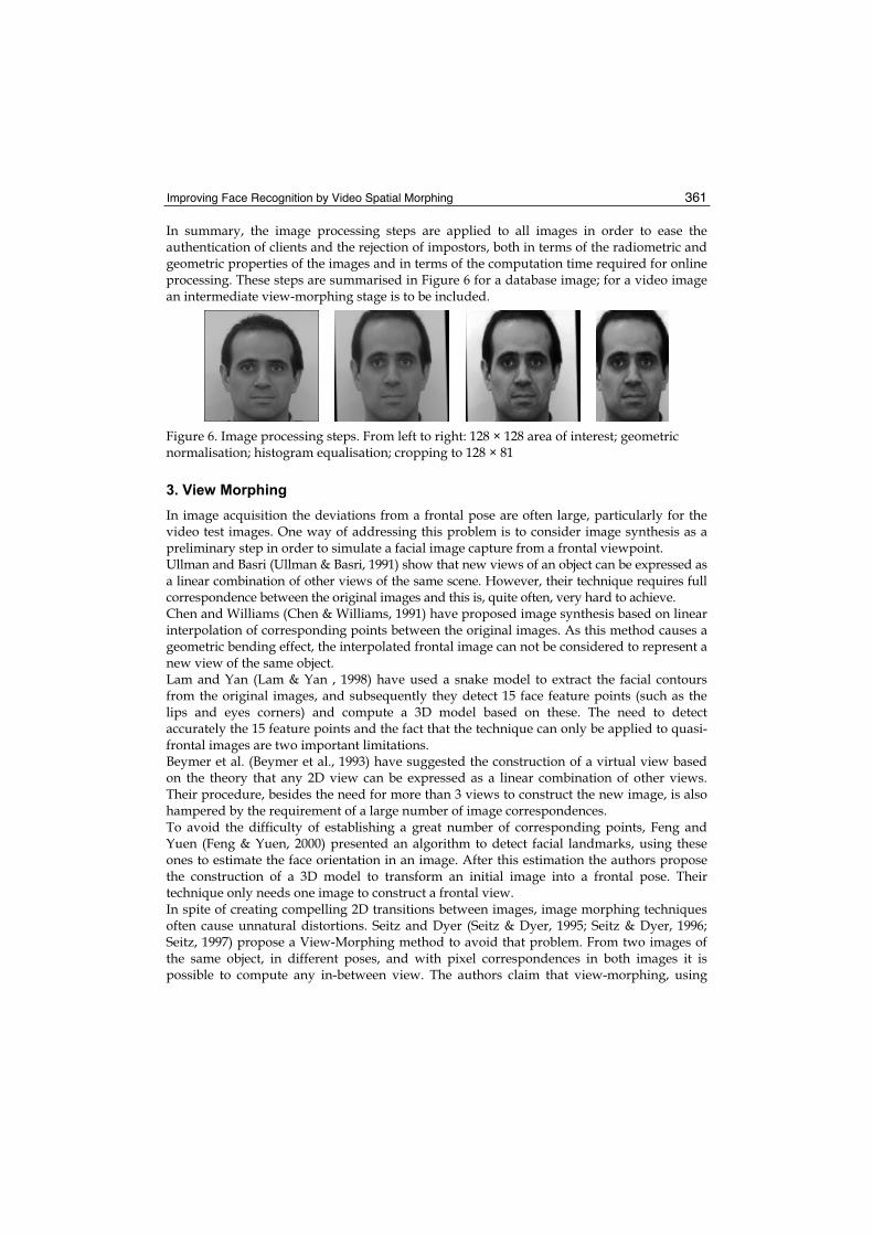
Improving Face Recognition by Video Spatial Morphing 361
In summary, the image processing steps are applied to all images in order to ease the authentication of clients and the rejection of impostors, both in terms of the radiometric and geometric properties of the images and in terms of the computation time required for online processing. These steps are summarised in Figure 6 for a database image; for a video image an intermediate view-morphing stage is to be included.
Figure 6. Image processing steps. From left to right: 128 × 128 area of interest; geometric normalisation; histogram equalisation; cropping to 128 × 81
3. View Morphing
In image acquisition the deviations from a frontal pose are often large, particularly for the video test images. One way of addressing this problem is to consider image synthesis as a preliminary step in order to simulate a facial image capture from a frontal viewpoint. Ullman and Basri (Ullman & Basri, 1991) show that new views of an object can be expressed as a linear combination of other views of the same scene. However, their technique requires full correspondence between the original images and this is, quite often, very hard to achieve. Chen and Williams (Chen & Williams, 1991) have proposed image synthesis based on linear interpolation of corresponding points between the original images. As this method causes a geometric bending effect, the interpolated frontal image can not be considered to represent a new view of the same object. Lam and Yan (Lam & Yan , 1998) have used a snake model to extract the facial contours from the original images, and subsequently they detect 15 face feature points (such as the lips and eyes corners) and compute a 3D model based on these. The need to detect accurately the 15 feature points and the fact that the technique can only be applied to quasi-frontal images are two important limitations. Beymer et al. (Beymer et al., 1993) have suggested the construction of a virtual view based on the theory that any 2D view can be expressed as a linear combination of other views. Their procedure, besides the need for more than 3 views to construct the new image, is also hampered by the requirement of a large number of image correspondences. To avoid the difficulty of establishing a great number of corresponding points, Feng and Yuen (Feng & Yuen, 2000) presented an algorithm to detect facial landmarks, using these ones to estimate the face orientation in an image. After this estimation the authors propose the construction of a 3D model to transform an initial image into a frontal pose. Their technique only needs one image to construct a frontal view. In spite of creating compelling 2D transitions between images, image morphing techniques often cause unnatural distortions. Seitz and Dyer (Seitz & Dyer, 1995; Seitz & Dyer, 1996; Seitz, 1997) propose a View-Morphing method to avoid that problem. From two images of the same object, in different poses, and with pixel correspondences in both images it is possible to compute any in-between view. The authors claim that view-morphing, using

Face Recognition 362
basic principles of projective geometry and image geometric interpolation yields a more realistic transition that preserves the underlying 3D geometry. This technique works by pre-warping two images prior to computing a morph and then by post-warping the interpolated images. Because no knowledge of 3D shape is required the technique may be applied to photographs and drawings, as well as rendered scenes. Xiao and Shah (Xiao & Shah, 2004) present an effective image-based approach without the explicit use of a 3D model. Based on the view-morphing methods, they propose a novel technique to synthesize a virtual view in a 2D space. Starting by establishing and refining corresponding feature points between each pair of images they determine the epipolar geometry for each pair and extract the trifocal plane by trifocal tensor computation. After marking a small number of feature lines, the correct dense disparity maps are obtained by using a triocular-stereo algorithm developed by them. Finally, after self-calibration of the three cameras, they can generate an arbitrary novel view, synthesized by the tri-view morphing algorithm. For our work we have developed a view-morphing algorithm closely following the Seitz and Dyer method. The view-morphing technique is shape-preserving, thus creating intermediate views that resemble the effect of rigid motion transformations in 3D. The intermediate images can be closer to any one of the two extreme images, this being controlled by a single transformation parameter.
Figure 7. The pre-warping, morphing, and post-warping stages of the view-morphing technique (adapted from Seitz, 1997)
For non-parallel original views, i.e. images obtained by cameras with non-parallel optical axes, the first step is to backproject those views into a single plane where they become parallel. This is done by using the adequate projection matrices, whose construction details are beyond the scope of this document. Considering Figure 7, the original images I0 and I1 are backprojected
C1
x
y
Î0
Î1
ÎS
C0
CS
I0
I1
IS
x
y
x
y
P
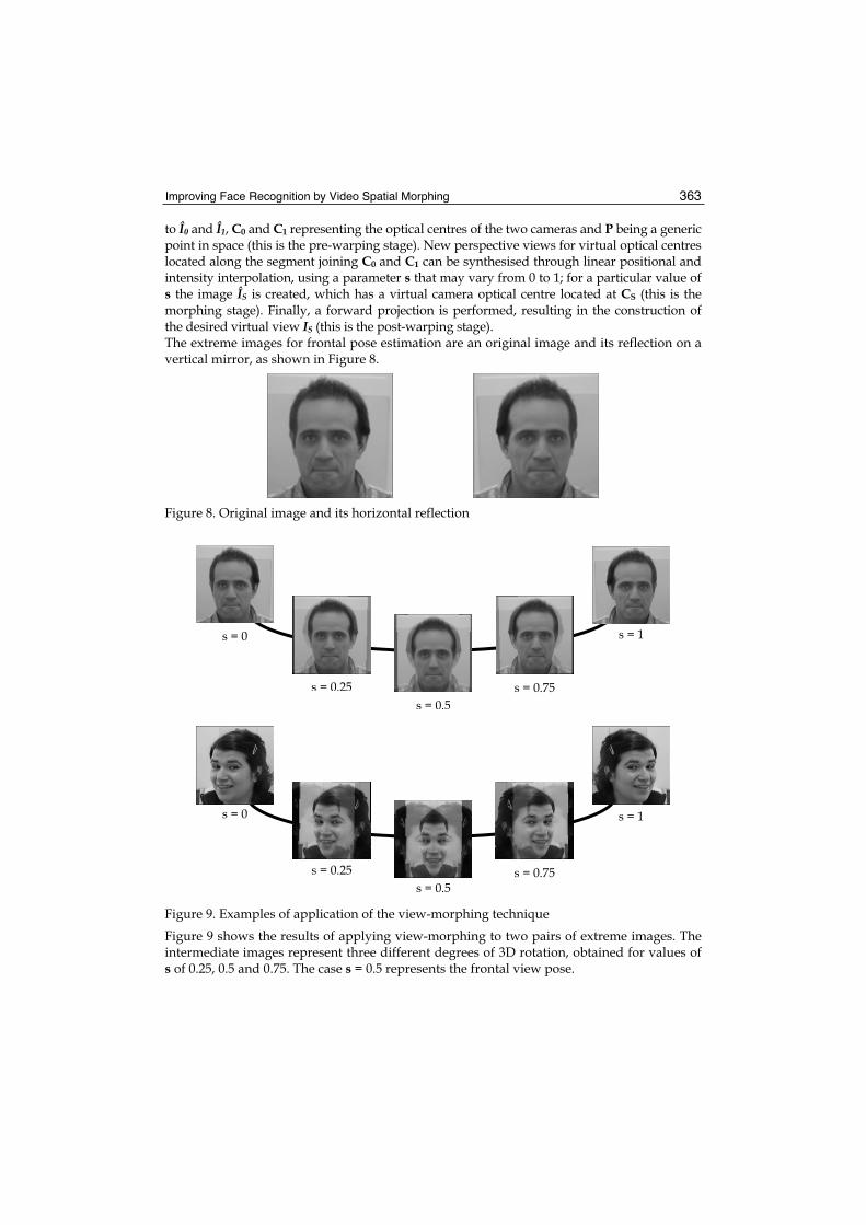
Improving Face Recognition by Video Spatial Morphing 363
to Î0 and Î1, C0 and C1 representing the optical centres of the two cameras and P being a generic point in space (this is the pre-warping stage). New perspective views for virtual optical centres located along the segment joining C0 and C1 can be synthesised through linear positional and intensity interpolation, using a parameter s that may vary from 0 to 1; for a particular value of s the image ÎS is created, which has a virtual camera optical centre located at CS (this is the morphing stage). Finally, a forward projection is performed, resulting in the construction of the desired virtual view IS (this is the post-warping stage). The extreme images for frontal pose estimation are an original image and its reflection on a vertical mirror, as shown in Figure 8.
Figure 8. Original image and its horizontal reflection
Figure 9. Examples of application of the view-morphing technique
Figure 9 shows the results of applying view-morphing to two pairs of extreme images. The intermediate images represent three different degrees of 3D rotation, obtained for values of s of 0.25, 0.5 and 0.75. The case s = 0.5 represents the frontal view pose.
s = 0
s = 0.25s = 0.5
s = 0.75
s = 1
s = 0
s = 0.25 s = 0.5
s = 0.75
s = 1

Face Recognition 364
Observe in Figure 9 that while the original male image is not far from a frontal view, the original female image is quite far from a frontal pose. As a consequence, a significant part of the synthesized views of the male individual is subjectively correct, whereas for the female individual only a small vertical strip of the image is satisfactory. The aforementioned problem is due to the practical implementation of the method, where only a few corresponding points in the original and reflected image were established, namely located on the eyes, nose and mouth, so that a very inaccurate extrapolation results in the outer vertical regions of the images.
4. Independent Component Analysis
Image recognition has been the objective of numerous studies and investigations in several scientific disciplines, giving rise to many different approaches of which we will only briefly review a few. Given the large data volumes present in image analysis, it is necessary to simplify the data by reducing its dimensionality. This goal can be reached through varied robust and efficient techniques, carrying out linear transformations that transform the data to a new co-ordinate system. The following representation, a linear statistical model, describes the observed data ( x ) through a mixing process (represented by matrix A ) that depends on the latent variables or sources s :
x As= (1)
However, in most problems the mixing matrix A is unknown. So, the independent variables must be recovered by a separation process (W is the separation matrix):
s W x= (2)
There are a lot of available methods to use for this purpose, namely second and higher order methods. Principal Component Analysis (PCA) and Common Factor Analysis (CFA) are methods that approximate the intrinsic structure of image data up to its second order statistics, assuming data gaussianity, and thus find a data representation using only the information in the covariance matrix. These methods are easier to implement than the higher order techniques (Hyvärinen, 1999). Nevertheless, the goal of many signal processing problems (such as speech enhancement, telecommunications and medical signal processing) is to reduce the information redundancy by exploiting the statistical structure of the data that is beyond second order. Independent Component Analysis (ICA) and Projection Pursuit (PP) are techniques that examine thoroughly the higher-order statistical structure in the data. Addressing higher-order statistical dependencies, these methods allow the separation of multivariate signals into additive sub-components, assuming the mutual statistical independence of the non-gaussian source signals (blind source separation is a special case of this), which is a much stronger condition than uncorrelatedness. Many authors have been using PCA for face recognition (Bartlett et al., 1998; Bartlett et al., 2002; Draper et al., 2003; Fortuna et al., 2002; Torres et al., 2000; Turk & Pentland, 1991). PCA consists in finding the principal components of the distribution of faces. These components are the eigenvectors of the covariance matrix of the database of facial images, each one accounting for a different amount of the variation among the images, such that the greatest

Improving Face Recognition by Video Spatial Morphing 365
variance of the data lies on the first co-ordinate (first principal component), the second greatest variance on the second co-ordinate, and so on. Each face can then be represented as a linear combination of the eigenfaces (eigenvectors) or approximated using only the “largest” eigenfaces, ordered according to the associated eigenvalues. (PCA is useful as a pre-processing step for other methods, as it reduces data dimensionality by keeping higher-order principal components and ignoring lower-order ones). Common Factor Analysis is used to explain variability among observed random variables, modelling those as linear combinations of a smaller number of unobserved random variables called factors. This method allows the identification of the relationships between data items and shows the similarities and differences between them. Simply stated, Projection Pursuit is a kind of statistical technique which involves finding the most “interesting” possible projections in multidimensional data. In the context of face recognition, ICA and NMF (Non-Negative Matrix Factorization) were analysed in (Rajapakse & Wyse, 2003). Both approaches yield a sparse representation of localized features (from human faces) and the authors discuss the strengths and weaknesses of each one. For use in face recognition, J. Yang et al. (Yang et al., 2004) developed a new Kernel Fisher Discriminant analysis (KFD) algorithm, called Complete KFD (CKFD), which is claimed to be simpler and more powerful than the existing KFD algorithms. There are also studies comparing the use of Spatial-Temporal Networks (STN) and Conditional Probability Networks (CPN) in human face recognition (A. Fernández-Caballero et al., 2001). These authors evaluate both techniques by testing, without any kind of pre-processing, 16 image faces with 6 different poses and expressions for each one. The results obtained with CPN slightly outperform those with STN. A simple application of Independent Component Analysis (ICA) is the “cocktail party problem”, where the underlying speech signals (sources) are separated from the mixed data consisting of people talking simultaneously in a room (a blind source separation problem). Many authors (Bartlett et al., 1998; Bartlett et al., 2002; Draper et al., 2003; Fortuna et al., 2002) have compared face recognition results under PCA and ICA, generally claiming that ICA provides better performance. Te-Won Lee and colleagues (Lee et al., 2000; Lee & Lewicki, 2002) apply ICA to find statistically significant structures in images construed by classes of image types, such as text overlapping with natural scenes, or the natural scene itself composed by diverse structures or textures. Developing what they called the ICA mixture model, the authors mould up the underlying image with a mixture model that can capture the different types of image textures in classes, categorizing the data into several mutually exclusive classes and assuming that the data in each class are generated by a linear combination of independent, non-Gaussian sources, as is the case with ICA. Jung et al. (Jung et al., 2001), in the context of basic brain research and medical diagnosis and treatment, apply ICA to analyse electroencephalographic (EEG), magnetoencephalographic (MEG) and functional magnetic resonance imaging (fMRI) recordings. Removing artefacts and separating/recovering sources of the brain signals from these recordings, ICA allows the identification of different types of generators of the EEG and its magnetic counterpart (the MEG) and can be used to analyse hemodynamic signals from the brain recorded by the fMRI. In general terms, ICA is a statistical method that finds the independent components (or sources) by maximizing the statistical independence of the estimated components, according

Face Recognition 366
to equation (1). Mutual Information and non-gaussianity (measured by kurtosis or by approximations to negentropy) are popular criteria for measuring statistical independence of signals. Typical algorithms for ICA use centring and whitening as pre-processing steps in order to reduce the complexity of the problem for the actual iterative algorithm. The Newton method, the gradient ascent method, Infomax and FastICA are possible algorithms for ICA (Hyvärinen, 1999; Hyvärinen & Oja, 2000; Hyvärinen et al., 2001). The ICA representation can be constructed under architectures I and II. The former considers images as random variables and pixels as observations, the second treats pixels as random variables and images as observations (Bartlett et al., 1998; Bartlett et al., 2001). Architecture II produces more global features while architecture I produces spatially localized features that are mostly influenced by small parts of the image, leading to better object recognition results. Based on reasons given in (Sebastião, 2006b) and detailed in (Sebastião, 2006a), we constructed the ICA representation considering architecture I and implemented it by the FastICA algorithm, using ( ) = tanh( )g y y as the objective function. The data, X , is first centred, i.e. made zero-mean, according to the following equation:
= −cX X μ (3)
where μ represents the data mean. Then the data is whitened (or sphered), meaning it is normalised with respect to the variance. The sphering matrix, V , is defined by the eigenvalues and eigenvectors matrices of the covariance matrix:
12- T=V ED E (4)
where E is the eigenvectors and D is the eigenvalues matrix of the covariance matrix .The data matrix X with zero-mean and covariance matrix equal to the identity matrix is obtained by the following transformation:
CX=VX =VAs=As (5)
where A is an orthogonal matrix. Thus, the problem of finding an arbitrary matrix A in the model given by equation (1) is reduced to the simpler problem of finding an orthogonal matrix A . For convenience the data matrix X will be renamed to X , in the sequel. The evaluation/comparison of the two image representations, one pertaining to the training set (the still database images) and the other to the test set (the view-morphed images extracted from the video sequence), was measured by the cosine distance, as suggested by Bartlett et al. (Bartlett et al., 1998):
( ) ( ) ( )( ) ( )
test train
test train
, 1T
T
j id i j
j i⋅
= −X XX X
(6)
where ( )test jX and ( )trainT iX represent the row vectors j and i of matrices testX and train
TX ,respectively.
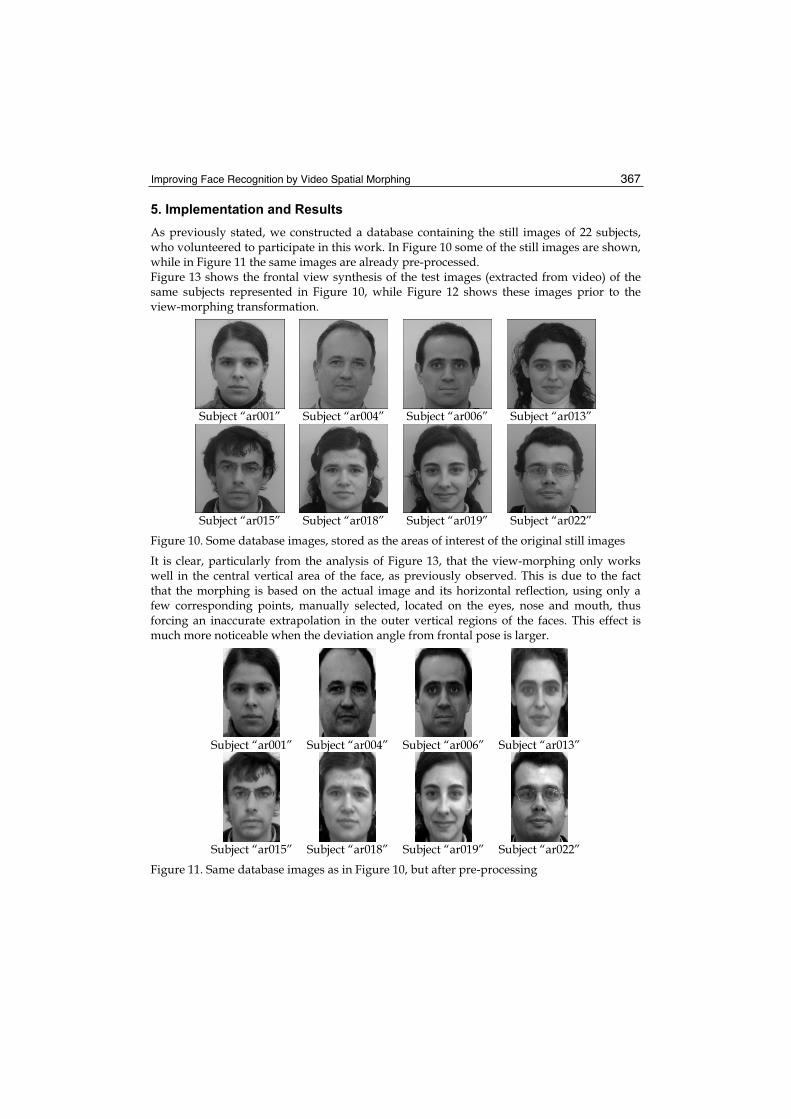
Improving Face Recognition by Video Spatial Morphing 367
5. Implementation and Results
As previously stated, we constructed a database containing the still images of 22 subjects, who volunteered to participate in this work. In Figure 10 some of the still images are shown, while in Figure 11 the same images are already pre-processed. Figure 13 shows the frontal view synthesis of the test images (extracted from video) of the same subjects represented in Figure 10, while Figure 12 shows these images prior to the view-morphing transformation.
Subject “ar001” Subject “ar004” Subject “ar006” Subject “ar013”
Subject “ar015” Subject “ar018” Subject “ar019” Subject “ar022” Figure 10. Some database images, stored as the areas of interest of the original still images
It is clear, particularly from the analysis of Figure 13, that the view-morphing only works well in the central vertical area of the face, as previously observed. This is due to the fact that the morphing is based on the actual image and its horizontal reflection, using only a few corresponding points, manually selected, located on the eyes, nose and mouth, thus forcing an inaccurate extrapolation in the outer vertical regions of the faces. This effect is much more noticeable when the deviation angle from frontal pose is larger.
Subject “ar001” Subject “ar004” Subject “ar006” Subject “ar013”
Subject “ar015” Subject “ar018” Subject “ar019” Subject “ar022” Figure 11. Same database images as in Figure 10, but after pre-processing
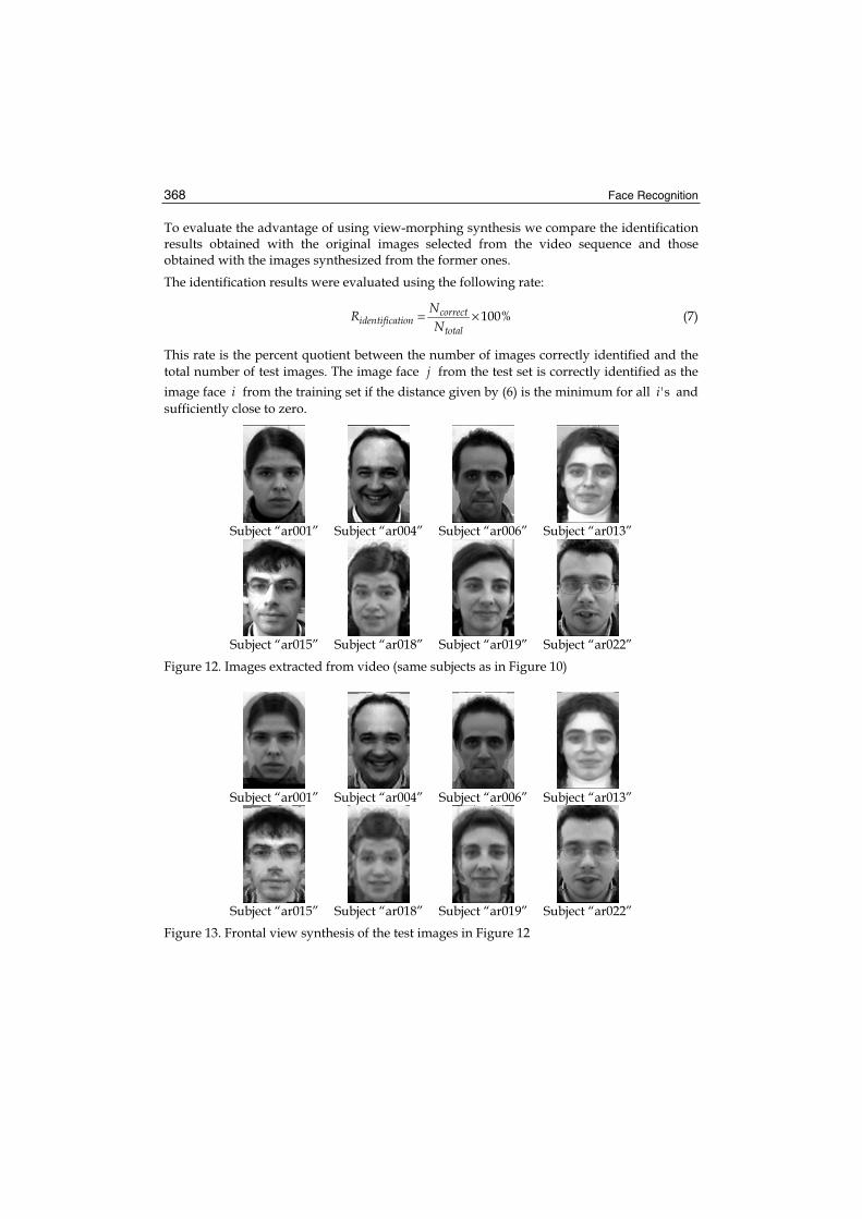
Face Recognition 368
To evaluate the advantage of using view-morphing synthesis we compare the identification results obtained with the original images selected from the video sequence and those obtained with the images synthesized from the former ones.
The identification results were evaluated using the following rate:
100%correctidentification
total
NRN
= × (7)
This rate is the percent quotient between the number of images correctly identified and the total number of test images. The image face j from the test set is correctly identified as the image face i from the training set if the distance given by (6) is the minimum for all 'si and sufficiently close to zero.
Subject “ar001” Subject “ar004” Subject “ar006” Subject “ar013”
Subject “ar015” Subject “ar018” Subject “ar019” Subject “ar022”
Figure 12. Images extracted from video (same subjects as in Figure 10)
Subject “ar001” Subject “ar004” Subject “ar006” Subject “ar013”
Subject “ar015” Subject “ar018” Subject “ar019” Subject “ar022” Figure 13. Frontal view synthesis of the test images in Figure 12

Improving Face Recognition by Video Spatial Morphing 369
To authenticate subjects we define a threshold for each individual using the distances of each face of subject i , selected from the video sequence, to all the representations in the training set. This threshold, for each individual, is given by:
i i iT = μ − σ (8)
where
( ) ( )
( )
images imagesind indN NN N 2k k i
k 1 j 1 k 1 j 1i i
images ind images ind
d i, j d i, j
andN N N .N 1= = = =
− μ
μ = σ =⋅ −
(9)
with imagesN 3= (3 frames from a video fragment) and indN 22= (total number of images
in the database). Moreover, a subject is authenticated if the distances between the representation of at least two of the three selected test images and the subject’s training set representation are lower than the threshold value. Comparing the identification results obtained with the view-morphed images and those obtained with the original images from the video sequence, we get the following rates:
Video Images View-morphed Images
Identification rate - identificationR 32 100%66
× 35 100%66
×
Table 1. Identification rates obtained for the video images and the view-morphed images
These results support the advantage of synthesizing frontal images with the view-morphing method, to achieve individual identification, even in the experimental case where the view-morphing synthesis is hampered by the uneven location of the corresponding points. The authentication of a subject takes approximately 8 seconds with code far from optimised, including full training of the database and test (using a 2.8 GHz Pentium 4 processor with 1.00 GB of RAM).
With the aim of improving image quality as well as the recognition rate, image pre-processing was applied to all images, using a photometric transformation and a geometric normalisation, as explained in section 2. Some of the pre-processed view-morphed images are shown below, in Figure 14.
Table 2 compares the identification results obtained with the view-morphed images without and with pre-processing.
Without pre-processing
With pre- processing
Identification rate - identificationR 35 100%66
× 40 100%66
×
Table 2. Identification rates obtained for the view-morphed images, with and without pre-processing

Face Recognition 370
Subject “ar001” Subject “ar004” Subject “ar006” Subject “ar013”
Subject “ar015” Subject “ar018” Subject “ar019” Subject “ar022” Figure 14. Sample pre-processed and view-morphed images (video frames)
The above results suggest that one should use the pre-processed view-morphed images to get the best identification results. This way, the database is formed by the pre-processed images in frontal and neutral pose, and every image extracted from the video fragments is also subject to the full pre-processing stage.
5.1 Authentication of Clients
To authenticate clients we use a simple criterion, namely: at least two of the three test images from a video fragment must be correctly identified (meaning that the identity announced by the client gives the correct match in the database – a distance smaller than the respective threshold). The thresholds that allow the decision are associated to each individual, as previously defined, so that if we want to add a new subject to the database or to remove another one it is necessary to perform a full training test in order to establish the new threshold value for each subject. Considering the above criterion, a full authentication test was conducted and an authentication rate (defined similarly to the identification rate) was computed in two situations: (a) test images without the geometric transformation step, and (b) test images with the geometric transformation step. Table 3 presents the results achieved.
Without geometric transformation
With geometric transformation
Authentication rate - authenticationR
15 100%22
× 22 100%22
×
Table 3. Authentication rates obtained for the full set of view-morphed images, with and without geometric transformation
The results in Table 3 stress the importance of the geometric transformation. On the other hand, the fact that an entirely correct authentication rate could be achieved should not be overstated. In fact, the decision thresholds definition was designed for the best performance with the existing test images (22 × 3 = 66 images), but it is not guaranteed that similar results would be achieved for other test images.

Improving Face Recognition by Video Spatial Morphing 371
Training Set
ar001 ar004 ar015 ar018 ar019 ar022
I1 I2 I3 I1 I2 I3 I1 I2 I3 I1 I2 I3 I1 I2 I3 I1 I2 I3 ar001 0,26 0,14 0,18 0,85 0,75 0,69 0,37 0,30 0,26 0,43 0,36 0,41 0,47 0,39 0,44 0,52 0,57 0,47
ar002 0,55 0,56 0,61 0,71 0,66 0,67 0,64 0,64 0,61 0,83 0,82 0,62 0,92 0,80 0,85 0,97 0,99 0,64
ar003 0,49 0,49 0,52 0,84 0,79 0,94 0,65 0,31 0,30 0,18 0,23 0,48 0,24 0,20 0,42 0,42 0,41 0,55
ar004 0,55 0,60 0,58 0,31 0,32 0,19 0,81 1,00 0,95 0,84 0,70 0,61 0,59 0,73 0,45 0,53 0,45 0,46
ar005 0,27 0,29 0,32 0,61 0,59 0,47 0,38 0,54 0,51 0,48 0,44 0,32 0,49 0,42 0,27 0,32 0,45 0,19
ar006 0,33 0,33 0,43 0,54 0,47 0,37 0,61 0,62 0,60 0,71 0,67 0,57 0,55 0,54 0,31 0,49 0,49 0,32
ar007 0,27 0,18 0,25 0,68 0,59 0,54 0,45 0,41 0,36 0,36 0,34 0,39 0,37 0,25 0,25 0,32 0,37 0,33
ar008 0,60 0,60 0,63 0,31 0,33 0,37 0,71 0,71 0,63 0,54 0,46 0,64 0,54 0,42 0,30 0,42 0,48 0,32
ar009 0,30 0,32 0,38 1,01 0,90 0,83 0,26 0,22 0,27 0,48 0,54 0,50 0,65 0,46 0,58 0,66 0,74 0,57
ar010 0,35 0,26 0,35 0,88 0,76 0,69 0,49 0,32 0,28 0,49 0,42 0,49 0,52 0,41 0,44 0,59 0,65 0,49
ar011 0,37 0,42 0,40 0,66 0,69 0,66 0,31 0,42 0,40 0,37 0,42 0,41 0,46 0,31 0,31 0,42 0,54 0,24
ar012 0,32 0,38 0,29 0,77 0,67 0,74 0,54 0,56 0,51 0,48 0,48 0,33 0,42 0,44 0,47 0,46 0,48 0,38
ar013 0,57 0,60 0,63 0,72 0,72 0,85 0,66 0,49 0,45 0,19 0,22 0,59 0,19 0,16 0,34 0,35 0,31 0,49
ar014 0,42 0,45 0,46 0,96 0,85 0,99 0,47 0,32 0,33 0,27 0,34 0,43 0,42 0,32 0,58 0,53 0,57 0,65
ar015 0,47 0,43 0,52 1,16 1,08 1,03 0,28 0,08 0,15 0,39 0,52 0,46 0,65 0,49 0,62 0,61 0,76 0,67
ar016 0,37 0,30 0,33 0,98 0,96 0,84 0,20 0,22 0,18 0,40 0,41 0,46 0,54 0,38 0,48 0,60 0,68 0,50
ar017 0,26 0,23 0,22 0,81 0,65 0,67 0,45 0,41 0,39 0,36 0,32 0,32 0,41 0,35 0,42 0,37 0,46 0,44
ar018 0,53 0,51 0,52 0,89 0,86 0,98 0,50 0,29 0,24 0,09 0,11 0,45 0,23 0,16 0,40 0,33 0,37 0,52
ar019 0,54 0,50 0,53 0,66 0,64 0,82 0,60 0,42 0,39 0,18 0,23 0,51 0,24 0,13 0,36 0,32 0,35 0,49
ar020 0,45 0,45 0,43 0,86 0,80 0,91 0,57 0,36 0,33 0,29 0,29 0,51 0,31 0,27 0,47 0,46 0,44 0,55
ar021 0,32 0,27 0,30 0,52 0,44 0,41 0,42 0,65 0,62 0,53 0,57 0,29 0,57 0,47 0,30 0,30 0,42 0,22
Test
Set
ar022 0,45 0,42 0,44 0,63 0,62 0,67 0,53 0,43 0,44 0,31 0,31 0,44 0,37 0,25 0,33 0,24 0,36 0,20
T= μ- 0,28 0,50 0,27 0,27 0,26 0,32 Table 4. Distances among the ICA representations of the view-morphed test images of some subjects and the representations of the training set formed by the database pre-processed images

Face Recognition 372
However, note also that, in practice, it is possible to extract much more than only three images from each video sequence, which will possibly increase the number of correct matches. In fact, it is in the essence of the adopted approach that the increased number of test images, while necessarily generating many false negatives which are un-consequential, will augment the probability of detecting a few true positives in the case where the identification should occur.Table 4 shows the distances between the ICA representations of the view-morphed images of some subjects and the representations of the training set formed by the database pre-processed images. The analysis of the distances between all of the ICA representations of the test set and all the representations of the training set, led us to verify that, with a control system constructed under the conditions previously established, all the clients are correctly authenticated, giving an authentication rate of 100%.
5.2 Rejection of impostors
We have also performed a sort of “leave-one-out” tests to evaluate the capacity and the accuracy that this system could have to automatically reject the access of impostors (subjects announcing themselves with a false identity). This type of tests consists on the construction of a training set with n 1− subjects (in our case, 21), and then evaluating the differences and similarities between the ICA representations of this set and the representations of the test set formed by the images of the subject that was left out. This procedure is repeated until all the individuals of the database have been left out. Considering that subject j is left out, a training set with the remaining subjects is constructed. The distances between the ICA representations of the j subject images and the representations of the training set allows the definition of a threshold given by:
2i i iT = μ − σ (10)
where iμ and iσ can be obtained by using equation (9) with imagesN 3= and indN 21= .
In this way, the impostors will be (wrongly) authenticated if the distances between the representation of at least two of the three selected images and a representation of any subject on the training set are lower than the threshold value given by equation (10). Table 5 shows the results obtained. With these results we can conclude that, using the threshold given by equation (10), no impostor can gain access. The previously mentioned computer takes about 12 seconds to construct the training set and to evaluate an impostor authentication. These results are valid considering each one of the 22 subjects as an impostor and the training set formed by the other 21. Aside from these results, it can also be observed that considering these 21 training sets and the threshold defined by equation (8), all the clients (the 21 individuals that formed the training sets) are correctly authenticated.
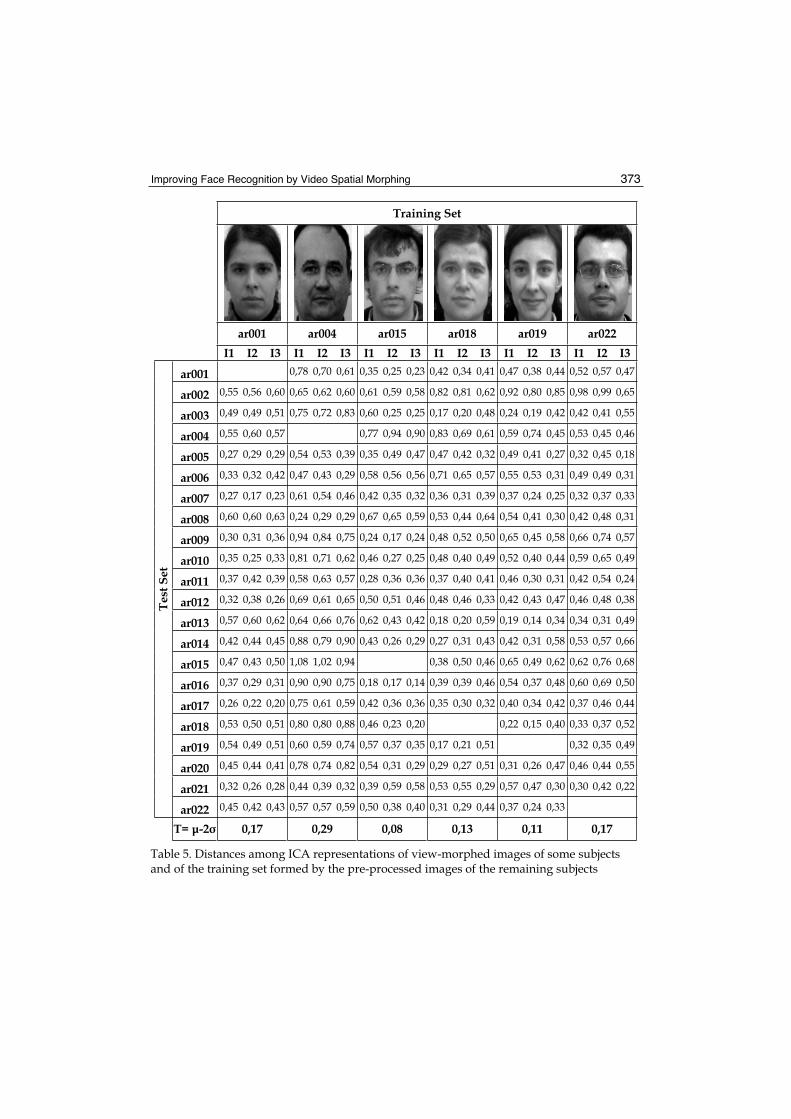
Improving Face Recognition by Video Spatial Morphing 373
Training Set
ar001 ar004 ar015 ar018 ar019 ar022 I1 I2 I3 I1 I2 I3 I1 I2 I3 I1 I2 I3 I1 I2 I3 I1 I2 I3
ar001 0,78 0,70 0,61 0,35 0,25 0,23 0,42 0,34 0,41 0,47 0,38 0,44 0,52 0,57 0,47
ar002 0,55 0,56 0,60 0,65 0,62 0,60 0,61 0,59 0,58 0,82 0,81 0,62 0,92 0,80 0,85 0,98 0,99 0,65
ar003 0,49 0,49 0,51 0,75 0,72 0,83 0,60 0,25 0,25 0,17 0,20 0,48 0,24 0,19 0,42 0,42 0,41 0,55
ar004 0,55 0,60 0,57 0,77 0,94 0,90 0,83 0,69 0,61 0,59 0,74 0,45 0,53 0,45 0,46
ar005 0,27 0,29 0,29 0,54 0,53 0,39 0,35 0,49 0,47 0,47 0,42 0,32 0,49 0,41 0,27 0,32 0,45 0,18
ar006 0,33 0,32 0,42 0,47 0,43 0,29 0,58 0,56 0,56 0,71 0,65 0,57 0,55 0,53 0,31 0,49 0,49 0,31
ar007 0,27 0,17 0,23 0,61 0,54 0,46 0,42 0,35 0,32 0,36 0,31 0,39 0,37 0,24 0,25 0,32 0,37 0,33
ar008 0,60 0,60 0,63 0,24 0,29 0,29 0,67 0,65 0,59 0,53 0,44 0,64 0,54 0,41 0,30 0,42 0,48 0,31
ar009 0,30 0,31 0,36 0,94 0,84 0,75 0,24 0,17 0,24 0,48 0,52 0,50 0,65 0,45 0,58 0,66 0,74 0,57
ar010 0,35 0,25 0,33 0,81 0,71 0,62 0,46 0,27 0,25 0,48 0,40 0,49 0,52 0,40 0,44 0,59 0,65 0,49
ar011 0,37 0,42 0,39 0,58 0,63 0,57 0,28 0,36 0,36 0,37 0,40 0,41 0,46 0,30 0,31 0,42 0,54 0,24
ar012 0,32 0,38 0,26 0,69 0,61 0,65 0,50 0,51 0,46 0,48 0,46 0,33 0,42 0,43 0,47 0,46 0,48 0,38
ar013 0,57 0,60 0,62 0,64 0,66 0,76 0,62 0,43 0,42 0,18 0,20 0,59 0,19 0,14 0,34 0,34 0,31 0,49
ar014 0,42 0,44 0,45 0,88 0,79 0,90 0,43 0,26 0,29 0,27 0,31 0,43 0,42 0,31 0,58 0,53 0,57 0,66
ar015 0,47 0,43 0,50 1,08 1,02 0,94 0,38 0,50 0,46 0,65 0,49 0,62 0,62 0,76 0,68
ar016 0,37 0,29 0,31 0,90 0,90 0,75 0,18 0,17 0,14 0,39 0,39 0,46 0,54 0,37 0,48 0,60 0,69 0,50
ar017 0,26 0,22 0,20 0,75 0,61 0,59 0,42 0,36 0,36 0,35 0,30 0,32 0,40 0,34 0,42 0,37 0,46 0,44
ar018 0,53 0,50 0,51 0,80 0,80 0,88 0,46 0,23 0,20 0,22 0,15 0,40 0,33 0,37 0,52
ar019 0,54 0,49 0,51 0,60 0,59 0,74 0,57 0,37 0,35 0,17 0,21 0,51 0,32 0,35 0,49
ar020 0,45 0,44 0,41 0,78 0,74 0,82 0,54 0,31 0,29 0,29 0,27 0,51 0,31 0,26 0,47 0,46 0,44 0,55
ar021 0,32 0,26 0,28 0,44 0,39 0,32 0,39 0,59 0,58 0,53 0,55 0,29 0,57 0,47 0,30 0,30 0,42 0,22
Test
Set
ar022 0,45 0,42 0,43 0,57 0,57 0,59 0,50 0,38 0,40 0,31 0,29 0,44 0,37 0,24 0,33
T= μ-2 0,17 0,29 0,08 0,13 0,11 0,17
Table 5. Distances among ICA representations of view-morphed images of some subjects and of the training set formed by the pre-processed images of the remaining subjects

Face Recognition 374
6. Conclusion
This work addressed the applicability of Independent Component Analysis to face recognition through image analysis, namely to the facial authentication problem. We defined and tested the main functionality of a potentially automatic vision system. In fact, some aspects of the process have been performed manually, but it is well known and the literature clearly documents successful automated methods for those operations. The main purpose of the system is to validate the clients’ access to restricted areas and to avoid the entrance of impostors, using as few restrictions on the environment as possible, and causing virtually no discomfort on the clients, both by not forcing them to multiple image acquisitions in the database construction phase, and by allowing them to walk naturally (with no specific pose for image capture) in the direction of the entrance. The results obtained have demonstrated the usefulness of the image pre-processing steps described and of the view-morphing techniques to generate virtual frontal views from slightly lateral images of the individuals. The identification of clients was 100% accurate, although it can be observed from the tables in the text that the robustness of the method is not high, as there is a significant number of “near” false-positives. On the other hand, the tests for the rejection of impostors have also proved that this most important goal could be successfully achieved for the data available. Nevertheless, because the two experiments were conducted separately, there are limits to the usability of the results, as is implied by the fact that the computation of the thresholds for identification and for rejection resulted different (that is, one and two standard deviations from mean). This indicates that further work must be done to counter this obvious limitation. One must take into consideration, however, that the building of the database was not thoroughly addressed, as timing constraints in the development phase of the work forced this process to be done very fast. The experience in analysing the results shows that test images of much higher quality can be acquired with only a minor investment in using one or two standard video cameras, and in setting up an adequate illumination and environment conditioning system, in particular to avoid specular reflections in the field of view.Also, the view-morphing point-correspondence problem was solved by manually setting the correspondences and, as previously pointed out, using only a small number of feature points located on a relatively narrow vertical strip of the faces. More accurate methods for matching pairs of points in an image and its reflection can be used in an automatic mode, not only for feature points but also for other points apart from the vertical symmetry line of the face, using epipolar geometry. As a final conclusion, one can say that the results achieved so far are quite encouraging and that the ideas for improving the methodology are well founded and promise a good outcome.

Improving Face Recognition by Video Spatial Morphing 375
7. References
Bartlett, M.; Lades, H. & Sejnowski, T. (1998). Independent Component Representations for Face Recognition, Proceedings of the SPIE Symposium on Electronic Imaging: Science and Technology; Human Vision and Electronic Imaging III, Vol. 3299, pp. 528-539, ISBN 9780819427397, California, July 1998, SPIE Press
Bartlett, M.; Movellan, J. & Sejnowski, T. (2002). Face Recognition by Independent Component Analysis, IEEE Transactions on Neural Networks, Vol. 13, No. 6, November 2002, pp. 1450-1464, ISSN 1045-9227
Beymer, D.; Shashua, A. & Poggio, T. (1993). Example based image analysis and synthesis, In A. I. Memo 1431, C. B. C. L: Paper No. 80, Artificial Intelligence Laboratory, MIT (November 1993)
Chen, S. & Williams, L. (1993). View Interpolation for Image Synthesis, Proceedings of the 20th Annual Conference on Computer Graphics and Interactive Techniques, pp. 279-288, ISBN 0-89791-601-8, California, August 1993, ACM Press, New York
Draper, B.; Baek, K.; Bartlett, M. & Beveridge, J. (2003). Recognizing faces with PCA and ICA, Computer Vision and Image Understanding, Vol. 91, No. 1-2, July 2003, pp. 115-137, ISSN 1077-3142
Feng, G. & Yuen, P. (2000). Recognition of Head-&-Shoulder Face Image Using Virtual Frontal-View Image, IEEE Transactions on Systems, Man, and Cybernetics-Part A: Cybernetics, Vol. 30, No. 6, November 2000, pp. 871-883, ISSN 1083–4427
Fernández-Caballero, A.; Gómez, F.; Moreno, J. & Fernández, M. (2001). Redes STN y CPN para el Reconocimiento de Rostros, Technical Report (in Spanish), Department of Computer Science, University of Castilla-La Mancha, 2001
Fortuna, J; Schuurman, D. & Capson, D (2002). A Comparison of PCA and ICA for Object Recognition Under Varying Illumination, Proceedings of the 16th International Conference on Pattern Recognition (ICPR’02), Vol. 3, pp. 11-15, ISBN 0-7695-1695-X, Canada, August 2002, IEEE Computer Society, Washington DC
Hyvärinen, A. (1999). Survey on Independent Component Analysis, Neural Computing Surveys, Vol. 2, 1999, pp. 94-128, ISSN 1093-7609
Hyvärinen, A. & Oja, E. (2000). Independent Component Analysis: Algorithms and Applications, Neural Networks, Vol. 13, No. 4-5, May-June 2000, pp. 411-430, ISSN 0893-6080
Hyvärinen, A.; Karhunen, J. & Oja, E. (2001). Independent Component Analysis, John Wiley & Sons, ISBN 978-0-471-40540-5, New York
Jung, T.-P.; Makeig, S; Mckeown, M.; Bell, A.; Lee, T.-W. & Sejnowski, T. (2001). Imaging Brain Dynamics Using Independent Component Analysis (Invited Paper). Proceedings of the IEEE, Vol. 89, No. 7, July 2001, pp. 1107-1122, ISSN 0018-9219
Lam, K. & Yan, H. (1998). An Analytic-to-Holistic Approach for Face Recognition Based on a Single Frontal View, IEEE Transactions on Pattern Analysis and Machine Intelligence,Vol. 20, No. 7, July 1998, pp. 673-686, ISSN 0162-8828
Lee, T.-W.; Lewicki, M. & Sejnowski, T. (2000). ICA mixture models for unsupervised classification with non-Gaussian classes and automatic context switching in blind signal separation, IEEE Transactions on Pattern Analysis and Machine Intelligence, Vol. 22, No. 10, October 2000, pp. 1078–1089, ISSN 0162-8828

Face Recognition 376
Lee T.-W. & Lewicki, M. (2002). Unsupervised Image Classification, Segmentation, and Enhancement Using ICA Mixture Models. IEEE Transactions on Image Processing,Vol. 11, No. 3, March 2002, pp. 270–279, ISSN 1057-7149
Rajapakse, M. & Wyse, L. (2003). NMF vs ICA for Face Recognition, Proceedings of the 3rd International Symposium on Image and Signal Processing and Analysis, pp. 605-610, ISBN 953-184-061-X, Italy, September 2003, IEEE Computer Society Press
Sebastião, R. (2006a). Autenticação de Faces a partir da Aquisição de Sequências de Imagens, MSc thesis (in Portuguese), Faculdade de Ciências e Faculdade de Engenharia da Universidade do Porto, Porto, Janeiro 2006
Sebastião, R.; Silva, J. & Padilha, A. (2006b). Face Recognition from Spatially-Morphed Video Sequences, Proceedings of International Conference on Image Analysis and Recognition,pp. 365-374, ISBN 3-540-44894-2, Póvoa de Varzim, September 2006, Springer LNCS 4142, Berlin
Seitz, S. & Dyer, C. (1995). Physically-valid View Synthesis by Image Interpolation, Proceedings of IEEE Workshop on Representations of Visual Scenes, pp. 18-25, ISBN 0-8186-7122-X, Massachusetts, June 1995, IEEE Computer Society Press
Seitz, S. & Dyer, C. (1996). View Morphing, Proceedings of the 23rd Annual Conference on Computer Graphics and Interactive Techniques (SIGGRAPH’96), pp. 21-30, ISBN 0-89791-746-4, New Orleans, August 1996, ACM Press, New York
Seitz, S. (1997). Image-Based Transformation of Viewpoint and Scene Appearance, PhD Thesis, University of Wisconsin–Madison, Madison, 1997
Torres, L.; Lorente, L. & Vila, J. (2000). Automatic Face Recognition of Video Sequences Using Self-eigenfaces, International Symposium on Image/video Communication over Fixed and Mobile Networks, Rabat, Morocco, April 2000
Turk, M. & Pentland, A. (1991). Eigenfaces for Recognition, Journal of Cognitive Neuroscience,Vol. 3, No. 1, Winter 1991, pp. 71–86
Ullman, S. & Basri, R. (1991). Recognition by Linear Combination of Models, IEEE Transactions on Pattern Analysis and Machine Intelligence, Vol. 13, No. 10, October 1991, pp. 992-1006, ISSN 0162-8828
Xiao, J. & Shah, M. (2004). Tri-view Morphing, Computer Vision and Image Understanding, Vol. 96, No. 3, December 2004, pp. 345-366, ISSN 1077-3142
Yang, J.; Frangia A. & Yang, J.-y. (2004). A new kernel Fisher discriminant algorithm with application to face recognition, Neurocomputing, Vol. 56, January 2004, pp. 415-421, ISSN 0925-2312
20
Machine Analysis of Facial Expressions
Maja Pantic 1 and Marian Stewart Bartlett 21 Computing Department, Imperial College London,
2 Inst. Neural Computation, University of California 1 UK, 2 USA
1. Human Face and Its Expression
The human face is the site for major sensory inputs and major communicative outputs. It houses the majority of our sensory apparatus as well as our speech production apparatus. It is used to identify other members of our species, to gather information about age, gender, attractiveness, and personality, and to regulate conversation by gazing or nodding. Moreover, the human face is our preeminent means of communicating and understanding somebody’s affective state and intentions on the basis of the shown facial expression (Keltner & Ekman, 2000). Thus, the human face is a multi-signal input-output communicative system capable of tremendous flexibility and specificity (Ekman & Friesen, 1975). In general, the human face conveys information via four kinds of signals. (a) Static facial signals represent relatively permanent features of the face, such as the bony
structure, the soft tissue, and the overall proportions of the face. These signals contribute to an individual’s appearance and are usually exploited for person identification.
(b) Slow facial signals represent changes in the appearance of the face that occur gradually over time, such as development of permanent wrinkles and changes in skin texture. These signals can be used for assessing the age of an individual. Note that these signals might diminish the distinctness of the boundaries of the facial features and impede recognition of the rapid facial signals.
(c) Artificial signals are exogenous features of the face such as glasses and cosmetics. These signals provide additional information that can be used for gender recognition. Note that these signals might obscure facial features or, conversely, might enhance them.
(d) Rapid facial signals represent temporal changes in neuromuscular activity that may lead to visually detectable changes in facial appearance, including blushing and tears. These (atomic facial) signals underlie facial expressions.
All four classes of signals contribute to person identification, gender recognition, attractiveness assessment, and personality prediction. In Aristotle’s time, a theory was proposed about mutual dependency between static facial signals (physiognomy) and personality: “soft hair reveals a coward, strong chin a stubborn person, and a smile a happy person”. Today, few psychologists share the belief about the meaning of soft hair and strong chin, but many believe that rapid facial signals (facial expressions) communicate emotions (Ekman & Friesen, 1975; Ambady & Rosenthal, 1992; Keltner & Ekman, 2000) and personality traits (Ambady & Rosenthal, 1992). More specifically, types of messages

Face Recognition 378
communicated by rapid facial signals include the following (Ekman & Friesen, 1969; Pantic et al., 2006): (a) affective / attitudinal states and moods,1 e.g., joy, fear, disbelief, interest, dislike, stress, (b) emblems, i.e., culture-specific communicators like wink, (c) manipulators, i.e., self-manipulative actions like lip biting and yawns, (d) illustrators, i.e., actions accompanying speech such as eyebrow flashes, (e) regulators, i.e., conversational mediators such as the exchange of a look, head nodes
and smiles.
1.1 Applications of Facial Expression Measurement Technology
Given the significant role of the face in our emotional and social lives, it is not surprising that the potential benefits from efforts to automate the analysis of facial signals, in particular rapid facial signals, are varied and numerous (Ekman et al., 1993), especially when it comes to computer science and technologies brought to bear on these issues (Pantic, 2006). As far as natural interfaces between humans and computers (PCs / robots / machines) are concerned, facial expressions provide a way to communicate basic information about needs and demands to the machine. In fact, automatic analysis of rapid facial signals seem to have a natural place in various vision sub-systems, including automated tools for tracking gaze and focus of attention, lip reading, bimodal speech processing, face / visual speech synthesis, and face-based command issuing. Where the user is looking (i.e., gaze tracking) can be effectively used to free computer users from the classic keyboard and mouse. Also, certain facial signals (e.g., a wink) can be associated with certain commands (e.g., a mouse click) offering an alternative to traditional keyboard and mouse commands. The human capability to “hear” in noisy environments by means of lip reading is the basis for bimodal (audiovisual) speech processing that can lead to the realization of robust speech-driven interfaces. To make a believable “talking head” (avatar) representing a real person, recognizing the person’s facial signals and making the avatar respond to those using synthesized speech and facial expressions is important. Combining facial expression spotting with facial expression interpretation in terms of labels like “did not understand”, “disagree”, “inattentive”, and “approves” could be employed as a tool for monitoring human reactions during videoconferences, web-based lectures, and automated tutoring sessions. Attendees’ facial expressions will inform the speaker (teacher) of the need to adjust the (instructional) presentation. The focus of the relatively recently initiated research area of affective computing lies on sensing, detecting and interpreting human affective states and devising appropriate means for handling this affective information in order to enhance current HCI designs (Picard, 1997). The tacit assumption is that in many situations human-machine interaction could be improved by the introduction of machines that can adapt to their users (think about computer-based advisors, virtual information desks, on-board computers and navigation systems, pacemakers, etc.). The information about when the existing processing should be 1 In contrast to traditional approach, which lists only (basic) emotions as the first type of messages conveyed by rapid facial signals (Ekman & Friesen, 1969), we treat this type of messages as being correlated not only to emotions but to other attitudinal states, social signals, and moods as well. We do so becuase cues identifying attitudinal states like interest and boredom, to those underlying moods, and to those disclosing social signaling like empathy and antipathy are all visualy detectable from someone’s facial expressions (Pantic et al., 2005, 2006).

Machine Analysis of Facial Expressions 379
adapted, the importance of such an adaptation, and how the processing/reasoning should be adapted, involves information about the how the user feels (e.g. confused, irritated, frustrated, interested). As facial expressions are our direct, naturally preeminent means of communicating emotions, machine analysis of facial expressions forms an indispensable part of affective HCI designs (Pantic & Rothkrantz, 2003; Maat & Pantic, 2006). Automatic assessment of boredom, fatigue, and stress, will be highly valuable in situations where firm attention to a crucial but perhaps tedious task is essential, such as aircraft and air traffic control, space flight and nuclear plant surveillance, or simply driving a ground vehicle like a truck, train, or car. If these negative affective states could be detected in a timely and unobtrusive manner, appropriate alerts could be provided, preventing many accidents from happening. Automated detectors of fatigue, depression and anxiety could form another step toward personal wellness technologies. Automating such assessment becomes increasingly important in an aging population to prevent medical practitioners from becoming overburdened. Monitoring and interpreting facial signals can also provide important information to lawyers, police, security, and intelligence agents regarding deception and attitude. Automated facial reaction monitoring could form a valuable tool in law enforcement, as now only informal interpretations are typically used. Systems that can recognize friendly faces or, more importantly, recognize unfriendly or aggressive faces and inform the appropriate authorities represent another application of facial measurement technology.
1.2 Outline of the Chapter
This chapter introduces recent advances in machine analysis of facial expressions. It first surveys the problem domain, describes the problem space, and examines the state of the art. Then it describes several techniques used for automatic facial expression analysis that were recently proposed by the authors. Four areas will receive particular attention: face detection, facial feature extraction, facial muscle action detection, and emotion recognition. Finally, some of the scientific and engineering challenges are discussed and recommendations for achieving a better facial expression measurement technology are outlined.
2. Automatic Facial Expression Analysis: Problem Space and State of the Art
Because of its practical importance explained above and the theoretical interest of cognitive and medical scientists (Ekman et al., 1993; Young, 1998; Cohen, 2006), machine analysis of facial expressions attracted the interest of many researchers. However, although humans detect and analyze faces and facial expressions in a scene with little or no effort, development of an automated system that accomplishes this task is rather difficult.
2.1 Level of Description: Action Units and Emotions
Two main streams in the current research on automatic analysis of facial expressions consider facial affect (emotion) detection and facial muscle action (action unit) detection. For exhaustive surveys of the related work, readers are referred to: Samal & Iyengar (1992) for an overview of early works, Tian et al. (2005) and Pantic (2006) for surveys of techniques for detecting facial muscle actions, and Pantic and Rothkrantz (2000, 2003) for surveys of facial affect recognition methods.

Face Recognition 380
Figure 1. Prototypic facial expressions of six basic emotions: anger, surprise, sadness, disgust, fear, and happiness
These two streams stem directly from two major approaches to facial expression measurement in psychological research (Cohn, 2006): message and sign judgment. The aim of message judgment is to infer what underlies a displayed facial expression, such as affect or personality, while the aim of sign judgment is to describe the “surface” of the shown behavior, such as facial movement or facial component shape. Thus, a brow furrow can be judged as “anger” in a message-judgment and as a facial movement that lowers and pulls the eyebrows closer together in a sign-judgment approach. While message judgment is all about interpretation, sign judgment attempts to be objective, leaving inference about the conveyed message to higher order decision making. As indicated by Cohn (2006), most commonly used facial expression descriptors in message judgment approaches are the six basic emotions (fear, sadness, happiness, anger, disgust, surprise; see Figure 1), proposed by Ekman and discrete emotion theorists, who suggest that these emotions are universally displayed and recognized from facial expressions (Keltner & Ekman, 2000). This trend can also be found in the field of automatic facial expression analysis. Most facial expressions analyzers developed so far target human facial affect analysis and attempt to recognize a small set of prototypic emotional facial expressions like happiness and anger (Pantic et al., 2005a). Automatic detection of the six basic emotions in posed, controlled displays can be done with reasonably high accuracy. However detecting these facial expressions in the less constrained environments of real applications is a much more challenging problem which is just beginning to be explored. There have also been a few tentative efforts to detect cognitive and psychological states like interest (El Kaliouby & Robinson, 2004), pain (Bartlett et al., 2006), and fatigue (Gu & Ji, 2005). In sign judgment approaches (Cohn & Ekman, 2005), a widely used method for manual labeling of facial actions is the Facial Action Coding System (FACS; Ekman & Friesen, 1978, Ekman et al., 2002). FACS associates facial expression changes with actions of the muscles that produce them. It defines 44 different action units (AUs), which are considered to be the smallest visually discernable facial movements (e.g, see Figure 2). FACS also provides the rules for recognition of AUs’ temporal segments (onset, apex and offset) in a face video. Using FACS, human coders can manually code nearly any anatomically possible facial display, decomposing it into the AUs and their temporal segments that produced the display. As AUs are independent of interpretation, they can be used for any higher order decision making process including recognition of basic emotions (Ekman et al., 2002), cognitive states like (dis)agreement and puzzlement (Cunningham et al., 2004), psychological states like suicidal depression (Heller & Haynal, 1997) or pain (Williams, 2002; Craig et al., 1991), and social signals like emblems (i.e., culture-specific interactive signals like wink), regulators (i.e., conversational mediators like nod and smile), and illustrators
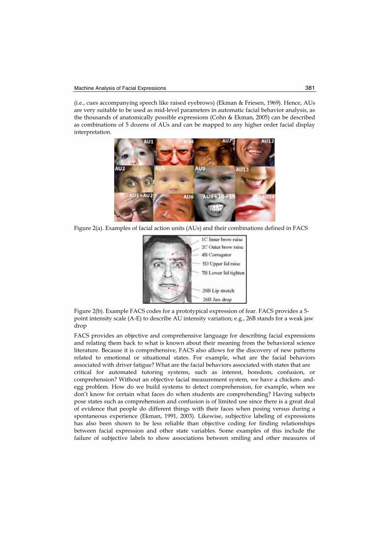
Machine Analysis of Facial Expressions 381
(i.e., cues accompanying speech like raised eyebrows) (Ekman & Friesen, 1969). Hence, AUs are very suitable to be used as mid-level parameters in automatic facial behavior analysis, as the thousands of anatomically possible expressions (Cohn & Ekman, 2005) can be described as combinations of 5 dozens of AUs and can be mapped to any higher order facial display interpretation.
Figure 2(a). Examples of facial action units (AUs) and their combinations defined in FACS
Figure 2(b). Example FACS codes for a prototypical expression of fear. FACS provides a 5-point intensity scale (A-E) to describe AU intensity variation; e.g., 26B stands for a weak jaw drop
FACS provides an objective and comprehensive language for describing facial expressions and relating them back to what is known about their meaning from the behavioral science literature. Because it is comprehensive, FACS also allows for the discovery of new patterns related to emotional or situational states. For example, what are the facial behaviors associated with driver fatigue? What are the facial behaviors associated with states that are critical for automated tutoring systems, such as interest, boredom, confusion, or comprehension? Without an objective facial measurement system, we have a chicken- and-egg problem. How do we build systems to detect comprehension, for example, when we don’t know for certain what faces do when students are comprehending? Having subjects pose states such as comprehension and confusion is of limited use since there is a great deal of evidence that people do different things with their faces when posing versus during a spontaneous experience (Ekman, 1991, 2003). Likewise, subjective labeling of expressions has also been shown to be less reliable than objective coding for finding relationships between facial expression and other state variables. Some examples of this include the failure of subjective labels to show associations between smiling and other measures of

Face Recognition 382
happiness, and it was not until FACS coding was introduced that a strong relationship was found, namely that expressions containing an eye region movement in addition to the mouth movement (AU12+6) were correlated with happiness, but expressions just containing the mouth smile (AU12) did not (Ekman, 2003). Another example where subjective judgments of expression failed to find relationships which were later found with FACS is the failure of naive subjects to differentiate deception and intoxication from facial display, whereas reliable differences were shown with FACS (Sayette et al., 1992). Research based upon FACS has also shown that facial actions can show differences between those telling the truth and lying at a much higher accuracy level than naive subjects making subjective judgments of the same faces (Frank & Ekman, 2004). Objective coding with FACS is one approach to the problem of developing detectors for state variables such as comprehension and confusion, although not the only one. Machine learning of classifiers from a database of spontaneous examples of subjects in these states is another viable approach, although this carries with it issues of eliciting the state, and assessment of whether and to what degree the subject is experiencing the desired state. Experiments using FACS face the same challenge, although computer scientists can take advantage of a large body of literature in which this has already been done by behavioral scientists. Once a database exists, however, in which a state has been elicited, machine learning can be applied either directly to image primitives, or to facial action codes. It is an open question whether intermediate representations such as FACS are the best approach to recognition, and such questions can begin to be addressed with databases such as the ones described in this chapter. Regardless of which approach is more effective, FACS provides a general purpose representation that can be useful for many applications. It would be time consuming to collect a new database and train application-specific detectors directly from image primitives for each new application. The speech recognition community has converged on a strategy that combines intermediate representations from phoneme detectors plus context-dependent features trained directly from the signal primitives, and perhaps a similar strategy will be effective for automatic facial expression recognition. It is not surprising, therefore, that automatic AU coding in face images and face image sequences attracted the interest of computer vision researchers. Historically, the first attempts to encode AUs in images of faces in an automatic way were reported by Bartlett et al. (1996), Lien et al. (1998), and Pantic et al. (1998). These three research groups are still the forerunners in this research field. The focus of the research efforts in the field was first on automatic recognition of AUs in either static face images or face image sequences picturing facial expressions produced on command. Several promising prototype systems were reported that can recognize deliberately produced AUs in either (near-) frontal view face images (Bartlett et al., 1999; Tian et al., 2001; Pantic & Rothkrantz, 2004a) or profile view face images (Pantic & Rothkrantz, 2004a; Pantic & Patras, 2006). These systems employ different approaches including expert rules and machine learning methods such as neural networks, and use either feature-based image representations (i.e., use geometric features like facial points; see section 5) or appearance-based image representations (i.e., use texture of the facial skin including wrinkles and furrows; see section 6). One of the main criticisms that these works received from both cognitive and computer scientists, is that the methods are not applicable in real-life situations, where subtle changes in facial expression typify the displayed facial behavior rather than the exaggerated changes that typify posed expressions. Hence, the focus of the research in the field started to shift to

Machine Analysis of Facial Expressions 383
automatic AU recognition in spontaneous facial expressions (produced in a reflex-like manner). Several works have recently emerged on machine analysis of AUs in spontaneous facial expression data (Cohn et al., 2004; Bartlett et al., 2003, 2005, 2006; Valstar et al., 2006). These methods employ probabilistic, statistical, and ensemble learning techniques, which seem to be particularly suitable for automatic AU recognition from face image sequences (Tian et al., 2005; Bartlett et al., 2006).
2.2 Posed vs. Spontaneous Facial Displays
The importance of making a clear distinction between spontaneous and deliberately displayed facial behavior for developing and testing computer vision systems becomes apparent when we examine the neurological substrate for facial expression. There are two distinct neural pathways that mediate facial expressions, each one originating in a different area of the brain. Volitional facial movements originate in the cortical motor strip, whereas the more involuntary, emotional facial actions, originate in the subcortical areas of the brain (e.g. Meihlke, 1973). Research documenting these differences was sufficiently reliable to become the primary diagnostic criteria for certain brain lesions prior to modern imaging methods (e.g. Brodal, 1981.) The facial expressions mediated by these two pathways have differences both in which facial muscles are moved and in their dynamics (Ekman, 1991; Ekman & Rosenberg, 2005). Subcortically initiated facial expressions (the involuntary group) are characterized by synchronized, smooth, symmetrical, consistent, and reflex-like facial muscle movements whereas cortically initiated facial expressions are subject to volitional real-time control and tend to be less smooth, with more variable dynamics (Rinn, 1984; Ekman & Rosenberg, 2005). However, precise characterization of spontaneous expression dynamics has been slowed down by the need to use non-invasive technologies (e.g. video), and the difficulty of manually coding expression intensity frame-by-frame. Thus the importance of video based automatic coding systems. Furthermore, the two pathways appear to correspond to the distinction between biologically driven versus socially learned facial behavior (Bartlett et al., 2006). Researchers agree, for the most part, that most types of facial expressions are learned like language, displayed under conscious control, and have culturally specific meanings that rely on context for proper interpretation (Ekman, 1989). Thus, the same lowered eyebrow expression that would convey “uncertainty” in North America might convey ”no” in Borneo (Darwin, 1872/1998). On the other hand, there are a limited number of distinct facial expressions of emotion that appear to be biologically wired, produced involuntarily, and whose meanings are similar across all cultures; for example, anger, contempt, disgust, fear, happiness, sadness, and surprise (see section 2.1). There are also spontaneous facial movements that accompany speech. These movements are smooth and ballistic, and are more typical of the subcortical system associated with spontaneous expressions (e.g. Rinn, 1984). There is some evidence that arm-reaching movements transfer from one motor system when they require planning to another when they become automatic, with different dynamic characteristics between the two (Torres & Anderson, 2006). It is unknown whether the same thing happens with learned facial displays. An automated system would enable exploration of such research questions. As already mentioned above, few works have been recently reported on machine analysis of spontaneous facial expression data (Cohn et al., 2004; Bartlett et al., 2003, 2005, 2006; Valstar et al., 2006). Except of the method for discerning genuine from fake facial expressions of pain described in section 7.3, the only reported effort to automatically discern spontaneous

Face Recognition 384
from deliberately displayed facial behavior is that of Valstar et al. (2006). It concerns an automated system for distinguishing posed from spontaneous brow actions (i.e. AU1, AU2, AU4, and their combinations). Conforming with the research findings in psychology, the system was built around characteristics of temporal dynamics of brow actions and employs parameters like speed, intensity, duration, and the occurrence order of brow actions to classify brow actions present in a video as either deliberate or spontaneous facial actions.
2.3 Facial Expression Configuration and Dynamics
Automatic recognition of facial expression configuration (in terms of AUs constituting the observed expression) has been the main focus of the research efforts in the field. However, both the configuration and the dynamics of facial expressions (i.e., the timing and the duration of various AUs) are important for interpretation of human facial behavior. The body of research in cognitive sciences, which argues that the dynamics of facial expressions are crucial for the interpretation of the observed behavior, is ever growing (Basilli, 1978; Russell & Fernandez-Dols, 1997; Ekman & Rosenberg, 2005; Ambadar et al., 2005). Facial expression temporal dynamics are essential for categorization of complex psychological states like various types of pain and mood (Williams, 2002). They represent a critical factor for interpretation of social behaviors like social inhibition, embarrassment, amusement, and shame (Keltner, 1997; Costa t al., 2001). They are also a key parameter in differentiation between posed and spontaneous facial displays (Ekman & Rosenberg, 2005). For instance, spontaneous smiles are smaller in amplitude, longer in total duration, and slower in onset and offset time than posed smiles (e.g., a polite smile) (Ekman, 2003). Another study showed that spontaneous smiles, in contrast to posed smiles, can have multiple apexes (multiple rises of the mouth corners – AU12) and are accompanied by other AUs that appear either simultaneously with AU12 or follow AU12 within 1s (Cohn & Schmidt, 2004). Similarly, it has been shown that the differences between spontaneous and deliberately displayed brow actions (AU1, AU2, AU4) is in the duration and the speed of onset and offset of the actions and in the order and the timing of actions’ occurrences (Valstar et al. 2006). In spite of these findings, the vast majority of the past work in the field does not take dynamics of facial expressions into account when analyzing shown facial behavior. Some of the past work in the field has used aspects of temporal dynamics of facial expression such as the speed of a facial point displacement or the persistence of facial parameters over time (e.g., Zhang & Ji, 2005; Tong et al., 2006; Littlewort et al., 2006). However, only three recent studies analyze explicitly the temporal dynamics of facial expressions. These studies explore automatic segmentation of AU activation into temporal segments (neutral, onset, apex, offset) in frontal- (Pantic & Patras, 2005; Valstar & Pantic, 2006a) and profile-view (Pantic & Patras, 2006) face videos. The works of Pantic & Patras (2005, 2006) employ rule-based reasoning to encode AUs and their temporal segments. In contrast to biologically inspired learning techniques (such as neural networks), which emulate human unconscious problem solving processes, rule-based techniques are inspired by human conscious problem solving processes. However, studies in cognitive sciences, like the one on “thin slices of behavior” (Ambady & Rosenthal, 1992), suggest that facial displays are neither encoded nor decoded at an intentional, conscious level of awareness. They may be fleeting changes in facial appearance that we still accurately judge in terms of emotions or personality even from very brief observations. In turn, this finding suggests that learning techniques inspired by human unconscious problem solving may be more suitable for facial expression recognition than

Machine Analysis of Facial Expressions 385
those inspired by human conscious problem solving (Pantic et al., 2005a). Experimental evidence supporting this assumption for the case of prototypic emotional facial expressions was recently reported (Valstar & Pantic, 2006b). Valstar & Pantic (2006a) also presented experimental evidence supporting this assumption for the case of expression configuration detection and its temporal activation model (neutral onset apex offset) recognition.
2.4 Facial Expression Intensity, Intentionality and Context Dependency
Facial expressions can vary in intensity. By intensity we mean the relative degree of change in facial expression as compared to a relaxed, neutral facial expression. In the case of a smile, for example, the intensity of the expression can be characterized as the degree of upward and outward movement of the mouth corners, that is, as the degree of perceivable activity in the Zygomaticus Major muscle (AU12) away from its resting, relaxed state (Duchenne, 1862/1990; Ekman & Friesen, 1978). It has been experimentally shown that the expression decoding accuracy and the perceived intensity of the underlying affective state vary linearly with the physical intensity of the facial display (Hess et al., 1997). Hence, explicit analysis of expression intensity variation is very important for accurate expression interpretation, and is also essential to the ability to distinguish between spontaneous and posed facial behavior discussed in the previous sections. While FACS provides a 5-point intensity scale to describe AU intensity variation and enable manual quantification of AU intensity (Ekman et al. 2002; Figure 2(b)), fully automated methods that accomplish this task are yet to be developed. However, first steps toward this goal have been made. Some researchers described changes in facial expression that could be used to represent intensity variation automatically (Essa & Pentland, 1997; Kimura & Yachida, 1997; Lien et al., 1998), and an effort toward implicit encoding of intensity was reported by Zhang & Ji (2005). Automatic coding of intensity variation was explicitly compared to manual coding in Bartlett et al. (2003a; 2006). They found that the distance to the separating hyperplane in their learned classifiers correlated significantly with the intensity scores provided by expert FACS coders. Rapid facial signals do not usually convey exclusively one type of messages but may convey any of the types (e.g., blinking is usually a manipulator but it may be displayed in an expression of confusion). It is crucial to determine which type of message a shown facial expression communicates since this influences the interpretation of it (Pantic & Rothkrantz, 2003). For instance, squinted eyes may be interpreted as sensitivity of the eyes to bright light if this action is a reflex (a manipulator), as an expression of disliking if this action has been displayed when seeing someone passing by (affective cue), or as an illustrator of friendly anger on friendly teasing if this action has been posed (in contrast to being unintentionally displayed) during a chat with a friend, to mention just a few possibilities. To interpret an observed facial signal, it is important to know the context in which the observed signal has been displayed – where the expresser is (outside, inside, in the car, in the kitchen, etc.), what his or her current task is, are other people involved, and who the expresser is. Knowing the expresser is particularly important as individuals often have characteristic facial expressions and may differ in the way certain states (other than the basic emotions) are expressed. Since the problem of context-sensing is extremely difficult to solve (if possible at all) for a general case, pragmatic approaches (e.g., activity/application- and user-centered approach) should be taken when learning the grammar of human facial behavior (Pantic et al., 2005a, 2006). However, except for a few works on user-profiled interpretation of facial expressions like those of Fasel et al. (2004) and Pantic & Rothkrantz (2004b), virtually all existing automated

Face Recognition 386
facial expression analyzers are context insensitive. Although machine-context sensing, that is, answering questions like who is the user, where is he or she, and what is he or she doing, has witnessed recently a number of significant advances (Nock et al., 2004, Pantic et al. 2006), the complexity of this problem makes context-sensitive facial expression analysis a significant research challenge.
2.5 Facial Expression Databases and Ground Truth
To develop and evaluate facial behavior analyzers capable of dealing with different dimensions of the problem space as defined above, large collections of training and test data are needed (Pantic & Rothkrantz, 2003; Pantic et al., 2005a; Tian et al., 2005; Bartlett et al., 2006).Picard (1997) outlined five factors that influence affective data collection: (a) Spontaneous versus posed: Is the emotion elicited by a situation or stimulus that is
outside the subject's control or the subject is asked to elicit the emotion? (b) Lab setting versus real-world: Is the data recording taking place in a lab or the emotion
is recorded in the usual environment of the subject? (c) Expression versus feeling: Is the emphasis on external expression or on internal feeling? (d) Open recording versus hidden recording: Is the subject aware that he is being recorded? (e) Emotion-purpose versus other-purpose: Does the subject know that he is a part of an
experiment and the experiment is about emotion? A complete overview of existing, publicly available datasets that can be used in research on automatic facial expression analysis is given by Pantic et al. (2005b). In general, there is no comprehensive reference set of face images that could provide a basis for all different efforts in the research on machine analysis of facial expressions. Only isolated pieces of such a facial database exist. An example is the unpublished database of Ekman-Hager Facial Action Exemplars (Ekman et al., 1999). It has been used by several research groups (e.g., Bartlett et al., 1999; Tian et al., 2001) to train and test their methods for AU detection from frontal-view facial expression sequences. Another example is JAFFE database (Lyons et al., 1999), which contains in total 219 static images of 10 Japanese females displaying posed expressions of six basic emotions and was used for training and testing various existing methods for recognition of prototypic facial expressions of emotions (Pantic et al., 2003). An important recent contribution to the field is the Yin Facial Expression Database (Yin et al., 2006), which contains 3D range data for prototypical expressions at a variety of intensities. The Cohn-Kanade facial expression database (Kanade et al., 2000) is the most widely used database in research on automated facial expression analysis (Tian et al., 2005; Pantic et al., 2005a). This database contains image sequences of approximately 100 subjects posing a set of 23 facial displays, and contains FACS codes in addition to basic emotion labels. The release of this database to the research community enabled a large amount of research on facial expression recognition and feature tracking. Two main limitations of this facial expression data set are as follows. First, each recording ends at the apex of the shown expression, which limits research of facial expression temporal activation patterns (onset apex offset). Second, many recordings contain the date/time stamp recorded over the chin of the subject. This makes changes in the appearance of the chin less visible and motions of the chin difficult to track. To fill this gap, the MMI facial expression database was developed (Pantic et al., 2005b). It has two parts: a part containing deliberately displayed facial expressions and a part

Machine Analysis of Facial Expressions 387
containing spontaneous facial displays. The first part contains over 4000 videos as well as over 600 static images depicting facial expressions of single AU activation, multiple AU activations, and six basic emotions. It has profile as well as frontal views, and was FACS coded by two certified coders. The second part of the MMI facial expression database contains currently 65 videos of spontaneous facial displays, that were coded in terms of displayed AUs and emotions by two certified coders. Subjects were 18 adults 21 to 45 years old and 11 children 9 to 13 years old; 48% female, 66% Caucasian, 30% Asian and 4% African. The recordings of 11 children were obtained during the preparation of a Dutch TV program, when children were told jokes by a professional comedian or were told to mimic how they would laugh when something is not funny. The recordings contain mostly facial expressions of different kinds of laughter and were made in a TV studio, using a uniform background and constant lighting conditions. The recordings of 18 adults were made in subjects’ usual environments (e.g., home), where they were shown segments from comedies, horror movies, and fear-factor series. The recordings contain mostly facial expressions of different kinds of laughter, surprise, and disgust expressions, which were accompanied by (often large) head motions, and were made under variable lighting conditions. Although the MMI facial expression database is the most comprehensive database for research on automated facial expression analysis, it still lacks metadata for the majority of recordings when it comes to frame-based AU coding. Further, although the MMI database is probably the only publicly available dataset containing recordings of spontaneous facial behavior at present, it still lacks metadata about the context in which these recordings were made such the utilized stimuli, the environment in which the recordings were made, the presence of other people, etc. Another database of spontaneous facial expressions was collected at UT Dallas (O’Toole et al., 2005). Similarly to the second part of the MMI facial expression database, facial displays were elicited using film clips. In the case of the UT Dallas database, however, there is no concurrent measure of expression content beyond the stimulus category. Yet, since subjects often do not experience the intended emotion and sometimes experience another one (e.g., disgust or annoyance instead of humor), concurrent measure of expression content beyond the stimulus category is needed. In other words, as in the case of the second part of the MMI facial expression database, coding in terms of displayed AUs and emotions independently of the stimulus category is needed. Mark Frank, in collaboration with Javier Movellan and Marian Bartlett, has collected a dataset of spontaneous facial behavior in an interview paradigm with rigorous FACS coding (Bartlett et al. 2006). This datased, called the RU-FACS Spontaneous Expression Dataset, consists of 100 subjects participating in a ’false opinion’ paradigm. In this paradigm, subjects first fill out a questionnaire regarding their opinions about a social or political issue. Subjects are then asked to either tell the truth or take the opposite opinion on an issue where they rated strong feelings, and convince an interviewer they are telling the truth. Interviewers were retired police and FBI agents. A high-stakes paradigm was created by giving the subjects $50 if they succeeded in fooling the interviewer, whereas if they were caught they were told they would receive no cash, and would have to fill out a long and boring questionnaire. In practice, everyone received a minimum of $10 for participating, and no one had to fill out the questionnaire. This paradigm has been shown to elicit a wide range of emotional expressions as well as speech-related facial expressions. This dataset is particularly challenging both because of speech-related mouth movements, and also because

Face Recognition 388
of out-of-plane head rotations which tend to be present during discourse. Subjects faces were digitized by four synchronized Dragonfly cameras from Point Grey (frontal, two partial profiles at 30 degrees, and one view from below). Two minutes of each subject’s behavior is being FACS coded by two certified FACS coders. FACS codes include the apex frame as well as the onset and offset frame for each action unit (AU). To date, 33 subjects have been FACS-coded. This dataset will be made available to the research community once the FACS coding is completed. With the exception of these problems concerned with acquiring valuable data and the related ground truth, another important issue is how does one construct and administer such a large facial expression benchmark database. Except of the MMI facial expression database (Pantic et al., 2005b), which was built as a web-based direct-manipulation application, allowing easy access and easy search of the available images, the existing facial expression databases are neither easy to access nor easy to search. In general, once the permission for usage is issued, large, unstructured files of material are sent. Other related questions are the following. How does one facilitate reliable, efficient, and secure inclusion of objects constituting this database? How could the performance of a tested automated system be included into the database? How should the relationship between the performance and the database objects used in the evaluation be defined? Pantic et al. (2003, 2005a, 2005b) emphasized a number of specific, research and development efforts needed to address the aforementioned problems. Nonetheless, note that their list of suggestions and recommendations is not exhaustive of worthwhile contributions.
3. Face Detection
The first step in facial information processing is face detection, i.e., identification of all regions in the scene that contain a human face. The problem of finding faces should be solved regardless of clutter, occlusions, and variations in head pose and lighting conditions. The presence of non-rigid movements due to facial expression and a high degree of variability in facial size, color and texture make this problem even more difficult. Numerous techniques have been developed for face detection in still images (Yang et al., 2002; Li & Jain, 2005). However, most of them can detect only upright faces in frontal or near-frontal view. The efforts that had the greatest impact on the community (as measured by, e.g., citations) include the following. Rowley et al. (1998) used a multi-layer neural network to learn the face and non-face patterns from the intensities and spatial relationships of pixels in face and non-face images. Sung and Poggio (1998) proposed a similar method. They used a neural network to find a discriminant function to classify face and non-face patterns using distance measures. Moghaddam and Pentland (1997) developed a probabilistic visual learning method based on density estimation in a high-dimensional space using an eigenspace decomposition. The method was applied to face localization, coding and recognition. Pentland et al. (1994) developed a real-time, view-based and modular (by means of incorporating salient features such as the eyes and the mouth) eigenspace description technique for face recognition in variable pose. Another method that can handle out-of-plane head motions is the statistical method for 3D object detection proposed by Schneiderman and Kanade (2000). Other such methods, which have been recently proposed, include those of Huang and Trivedi (2004) and Wang and Ji (2004). Most of these methods emphasize statistical learning techniques and use appearance features.

Machine Analysis of Facial Expressions 389
Arguably the most commonly employed face detector in automatic facial expression analysis is the real-time face detector proposed by Viola and Jones (2004). This detector consists of a cascade of classifiers trained by AdaBoost. Each classifier employs integral image filters, also called “box filters,” which are reminiscent of Haar Basis functions, and can be computed very fast at any location and scale. This is essential to the speed of the detector. For each stage in the cascade, a subset of features is chosen using a feature selection procedure based on AdaBoost. There are several adapted versions of the Viola-Jones face detector and the one that is employed by the systems discussed in detail in this chapter was proposed by Fasel et al. (2005). It uses GentleBoost instead of AdaBoost. GentleBoost uses the continuous output of each filter rather than binarizing it. A description of Gentle Boost classification can be found in Friedman et al. (2000).
4. Facial Feature Extraction
After the presence of a face has been detected in the observed scene, the next step is to extract the information about the displayed facial signals. The problem of facial feature extraction from regions in the scene that contain a human face may be divided into at least three dimensions (Pantic & Rothkrantz, 2000): (a) Is temporal information used? (b) Are the features holistic (spanning the whole face) or analytic (spanning subparts of the
face)?(c) Are the features view- or volume based (2D/3D)? Given this glossary and if the goal is face recognition, i.e., identifying people by looking at their faces, most of the proposed approaches adopt 2D holistic static facial features. On the other hand, many approaches to automatic facial expression analysis adopt 2D analytic spatio-temporal facial features (Pantic & Rothkrantz, 2003). This finding is also consistent with findings from psychological research suggesting that the brain processes faces holistically rather than locally whilst it processes facial expressions locally (Bassili, 1978). What is, however, not entirely clear yet is whether information on facial expression is passed to the identification process to aid person recognition or not. Some experimental data suggest this (Martinez, 2003; Roark et al., 2003). For surveys of computer vision efforts aimed at face recognition, the readers are referred to: Zhao et al. (2003), Bowyer (2004), and Li and Jain (2005). Most of the existing facial expression analyzers are directed toward 2D spatiotemporal facial feature extraction, including the methods proposed by the authors and their respective research teams. The usually extracted facial features are either geometric features such as the shapes of the facial components (eyes, mouth, etc.) and the locations of facial fiducial points (corners of the eyes, mouth, etc.) or appearance features representing the texture of the facial skin including wrinkles, bulges, and furrows. Typical examples of geometric-feature-based methods are those of Gokturk et al. (2002), who used 19 point face mesh, of Chang et al. (2006), who used a shape model defined by 58 facial landmarks, and of Pantic and her collegues (Pantic & Rothkrantz, 2004; Pantic & Patras, 2006; Valstar & Pantic, 2006a), who used a set of facial characteristic points like the ones illustrated in Figure 3. Typical examples of hybrid, geometric- and appearance-feature-based methods are those of Tian et al. (2001), who used shape-based models of eyes, eyebrows and mouth and transient features like crows-feet wrinkles and nasolabial furrow, and of Zhang and Ji (2005), who

Face Recognition 390
used 26 facial points around the eyes, eyebrows, and mouth and the same transient features as Tian et al (2001). Typical examples of appearance-feature-based methods are those of Bartlett et al. (1999, 2005, 2006) and Guo and Dyer (2005), who used Gabor wavelets, of Anderson and McOwen (2006), who used a holistic, monochrome, spatial-ratio face template, and of Valstar et al. (2004), who used temporal templates. It has been reported that methods based on geometric features are often outperformed by those based on appearance features using, e.g., Gabor wavelets or eigenfaces (Bartlett et al., 1999). Certainly, this may depend on the classification method and/or machine learning approach which takes the features as input. Recent studies like that of Pantic & Patras (2006), Valstar and Pantic (2006a), and those presented in this chapter, show that in some cases geometric features can outperform appearance-based ones. Yet, it seems that using both geometric and appearance features might be the best choice in the case of certain facial expressions (Pantic & Patras, 2006).Few approaches to automatic facial expression analysis based on 3D face modelling have been recently proposed. Gokturk et al. (2002) proposed a method for recognition of facial signals like brow flashes and smiles based upon 3D deformations of the face tracked on stereo image streams using a 19-point face mesh and standard optical flow techniques. The work of Cohen et al. (2003) focuses on the design of Bayesian network classifiers for emotion recognition from face video based on facial features tracked by a method called Piecewise Bezier Volume Deformation tracking (Tao & Huang, 1998). This tracker employs an explicit 3D wireframe model consisting of 16 surface patches embedded in Bezier volumes. Cohn et al. (2004) focus on automatic analysis of brow actions and head movements from face video and use a cylindrical head model to estimate the 6 degrees of freedom of head motion (Xiao et al., 2003). Baker and his colleagues developed several algorithms for fitting 2D and combined 2D+3D Active Appearance Models to images of faces (Xiao et al., 2004; Gross et al., 2006), which can be used further for various studies concerning human facial behavior. 3D face modeling is highly relevant to the present goals due to its potential to produce view-independent facial signal recognition systems. The main shortcomings of the current methods concern the need of a large amount of manually annotated training data and an almost always required manual selection of landmark facial points in the first frame of the input video based on which the face model will be warped to fit the face. Automatic facial feature point detection of the kind explained in section 5 offers a solution to these problems.
5. Geometric Facial Feature Extraction and Tracking
5.1 Facial Characteristic Point Detection
Previous methods for facial feature point detection can be classified as either texture-based methods (modeling local texture around a given facial point) or texture- and shape-based methods (regarding the constellation of all facial points as a shape, which is learned from a set of labeled faces, and trying to fit the shape to any unknown face). A typical texture-based method is that of Holden & Owens (2002), who used log-Gabor wavelets, while a typical texture- and shape-based method is that of Chen et al. (2004), who applied AdaBoost to determine facial feature point candidates for each pixel in an input image and used a shape model as a filter to select the most possible position of feature points. Although these detectors can be used to localize 20 facial characteristic points illustrated in Figure 3, which are used by the facial expression analyzers developed by Pantic and her team (e.g., Pantic & Patras, 2006; Valstar & Pantic, 2006a), none performs the detection with
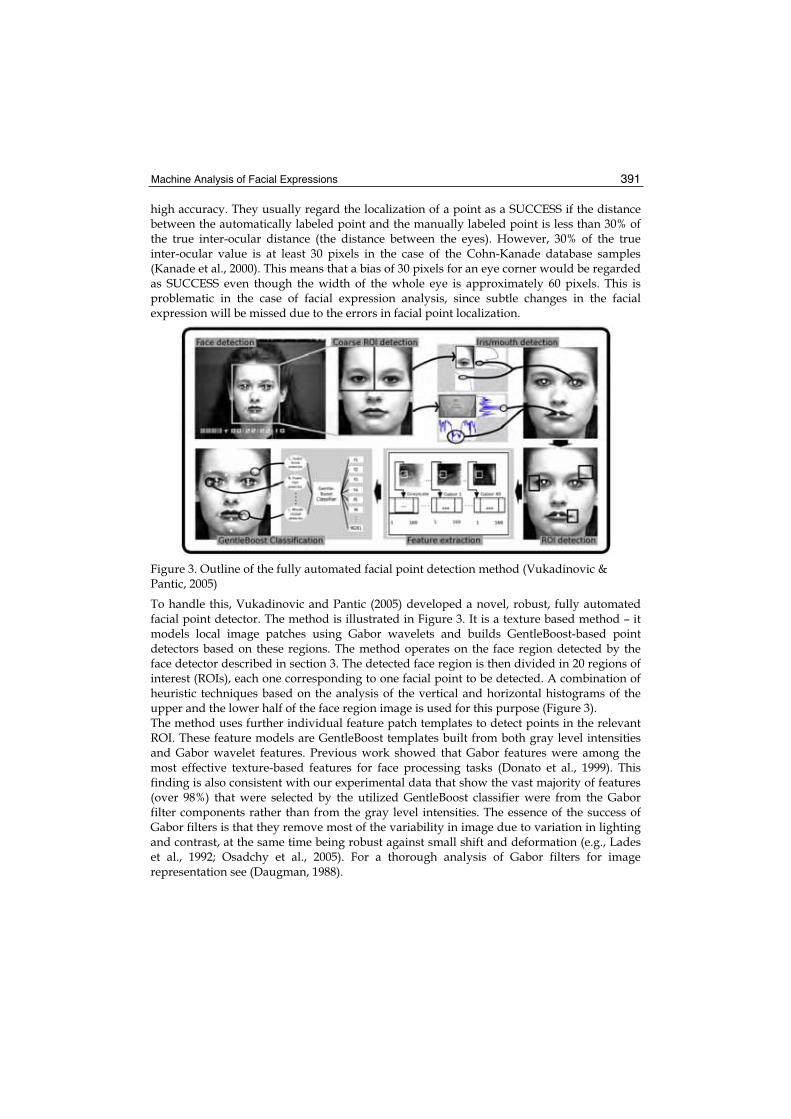
Machine Analysis of Facial Expressions 391
high accuracy. They usually regard the localization of a point as a SUCCESS if the distance between the automatically labeled point and the manually labeled point is less than 30% of the true inter-ocular distance (the distance between the eyes). However, 30% of the true inter-ocular value is at least 30 pixels in the case of the Cohn-Kanade database samples (Kanade et al., 2000). This means that a bias of 30 pixels for an eye corner would be regarded as SUCCESS even though the width of the whole eye is approximately 60 pixels. This is problematic in the case of facial expression analysis, since subtle changes in the facial expression will be missed due to the errors in facial point localization.
Figure 3. Outline of the fully automated facial point detection method (Vukadinovic & Pantic, 2005)
To handle this, Vukadinovic and Pantic (2005) developed a novel, robust, fully automated facial point detector. The method is illustrated in Figure 3. It is a texture based method – it models local image patches using Gabor wavelets and builds GentleBoost-based point detectors based on these regions. The method operates on the face region detected by the face detector described in section 3. The detected face region is then divided in 20 regions of interest (ROIs), each one corresponding to one facial point to be detected. A combination of heuristic techniques based on the analysis of the vertical and horizontal histograms of the upper and the lower half of the face region image is used for this purpose (Figure 3). The method uses further individual feature patch templates to detect points in the relevant ROI. These feature models are GentleBoost templates built from both gray level intensities and Gabor wavelet features. Previous work showed that Gabor features were among the most effective texture-based features for face processing tasks (Donato et al., 1999). This finding is also consistent with our experimental data that show the vast majority of features (over 98%) that were selected by the utilized GentleBoost classifier were from the Gabor filter components rather than from the gray level intensities. The essence of the success of Gabor filters is that they remove most of the variability in image due to variation in lighting and contrast, at the same time being robust against small shift and deformation (e.g., Lades et al., 1992; Osadchy et al., 2005). For a thorough analysis of Gabor filters for image representation see (Daugman, 1988).
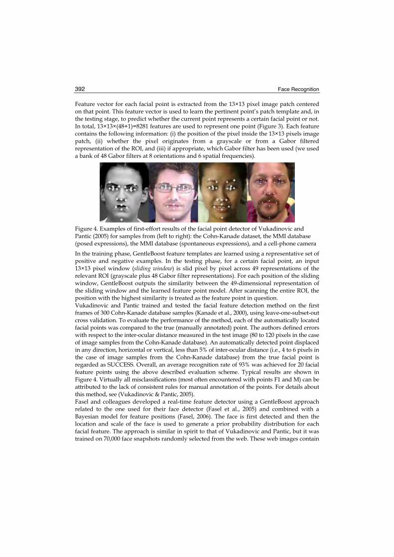
Face Recognition 392
Feature vector for each facial point is extracted from the 13×13 pixel image patch centered on that point. This feature vector is used to learn the pertinent point’s patch template and, in the testing stage, to predict whether the current point represents a certain facial point or not. In total, 13×13×(48+1)=8281 features are used to represent one point (Figure 3). Each feature contains the following information: (i) the position of the pixel inside the 13×13 pixels image patch, (ii) whether the pixel originates from a grayscale or from a Gabor filtered representation of the ROI, and (iii) if appropriate, which Gabor filter has been used (we used a bank of 48 Gabor filters at 8 orientations and 6 spatial frequencies).
Figure 4. Examples of first-effort results of the facial point detector of Vukadinovic and Pantic (2005) for samples from (left to right): the Cohn-Kanade dataset, the MMI database (posed expressions), the MMI database (spontaneous expressions), and a cell-phone camera
In the training phase, GentleBoost feature templates are learned using a representative set of positive and negative examples. In the testing phase, for a certain facial point, an input 13×13 pixel window (sliding window) is slid pixel by pixel across 49 representations of the relevant ROI (grayscale plus 48 Gabor filter representations). For each position of the sliding window, GentleBoost outputs the similarity between the 49-dimensional representation of the sliding window and the learned feature point model. After scanning the entire ROI, the position with the highest similarity is treated as the feature point in question. Vukadinovic and Pantic trained and tested the facial feature detection method on the first frames of 300 Cohn-Kanade database samples (Kanade et al., 2000), using leave-one-subset-out cross validation. To evaluate the performance of the method, each of the automatically located facial points was compared to the true (manually annotated) point. The authors defined errors with respect to the inter-ocular distance measured in the test image (80 to 120 pixels in the case of image samples from the Cohn-Kanade database). An automatically detected point displaced in any direction, horizontal or vertical, less than 5% of inter-ocular distance (i.e., 4 to 6 pixels in the case of image samples from the Cohn-Kanade database) from the true facial point is regarded as SUCCESS. Overall, an average recognition rate of 93% was achieved for 20 facial feature points using the above described evaluation scheme. Typical results are shown in Figure 4. Virtually all misclassifications (most often encountered with points F1 and M) can be attributed to the lack of consistent rules for manual annotation of the points. For details about this method, see (Vukadinovic & Pantic, 2005). Fasel and colleagues developed a real-time feature detector using a GentleBoost approach related to the one used for their face detector (Fasel et al., 2005) and combined with a Bayesian model for feature positions (Fasel, 2006). The face is first detected and then the location and scale of the face is used to generate a prior probability distribution for each facial feature. The approach is similar in spirit to that of Vukadinovic and Pantic, but it was trained on 70,000 face snapshots randomly selected from the web. These web images contain

Machine Analysis of Facial Expressions 393
greater pose and lighting variation than typical posed expression datasets, and were selected so that the machine learning systems could learn to be robust to such variations, and perform well in the less controlled image conditions of practical applications. When tested on such snapshots, the system obtains a median error of less than 0.05 interocular distance for eye positions, 0.06 for the nose tip, and 0.07 for the mouth center. For the strictly frontal subset of these web snapshots, which still contain substantial lighting variation, median error was 0.04, 0.045, and 0.05 interocular distance for eye, nose, and mouth position. This system could be combined with an approach such as that of Vukadinovic and Pantic to provide more robust initialization for the additional facial feature points.
5.2 Facial Point Tracking
Contractions of facial muscles induce movements of the facial skin and changes in the appearance of facial components such as the eyebrows, nose, and mouth. Since motion of the facial skin produces optical flow in the image, a large number of researchers have studied optical flow tracking (Pantic & Rothkrantz, 2000; 2003; Tian et al., 2005). The optical flow approach to describing face motion has the advantage of not requiring a facial feature extraction stage of processing. Dense flow information is available throughout the entire facial area, regardless of the existence of facial components, even in the areas of smooth texture such as the cheeks and the forehead. Because optical flow is the visible result of movement and is expressed in terms of velocity, it can be used to represent directly facial actions. One of the first efforts to utilize optical flow for recognition of facial expressions was the work of Mase (1991). Thereafter, many other researchers adopted this approach (Pantic & Rothkrantz, 2000; 2003; Tian et al., 2005). Standard optical flow techniques (e.g., Lucas & Kanade, 1981; Shi & Tomasi, 1994; Barron et al., 1994) are also most commonly used for tracking facial feature points. DeCarlo and Metaxas (1996) presented a model-based tracking algorithm in which a face shape model and motion estimation are integrated using optical flow and edge information. Gokturk et al. (2002) track the points of their 19-point face mesh on the stereo image streams using the standard Lucas-Kanade optical flow algorithm (Lucas & Kanade, 1981). To achieve facial feature point tracking Lien et al. (1998), Tian et al. (2001), and Cohn et al. (2004) used the standard Lucas-Kanade optical flow algorithm too. To realize fitting of 2D and combined 2D+3D Active Appearance Models to images of faces, Xiao et al. (2004) use an algorithm based on an "inverse compositional" extension to the Lucas-Kanade algorithm. To address the limitations inherent in optical flow techniques such as the accumulation of error and the sensitivity to noise, occlusion, clutter, and changes in illumination, several researchers used sequential state estimation techniques to track facial feature points in image sequences. Both, Zhang and Ji (2005) and Gu and Ji (2005) used facial point tracking based on a Kalman filtering scheme, which is the traditional tool for solving sequential state problems. The derivation of the Kalman filter is based on a state-space model (Kalman, 1960), governed by two assumptions: (i) linearity of the model and (ii) Gaussianity of both the dynamic noise in the process equation and the measurement noise in the measurement equation. Under these assumptions, derivation of the Kalman filter leads to an algorithm that propagates the mean vector and covariance matrix of the state estimation error in an iterative manner and is optimal in the Bayesian setting. To deal with the state estimation in nonlinear dynamical systems, the extended Kalman filter was proposed, which is derived through linearization of the state-space model. However, many of the state estimation

Face Recognition 394
problems, including human facial expression analysis, are nonlinear and quite often non-Gaussian too. Thus, if the face undergoes a sudden or rapid movement, the prediction of features positions from Kalman filtering will be significantly off. To handle this problem, Zhang and Ji (2005) and Gu and Ji (2005) used the information about the IR-camera detected pupil location together with the output of Kalman filtering to predict facial features positions in the next frame of an input face video. To overcome these limitations of the classical Kalman filter and its extended form in general, particle filters wereproposed. For an extended overview of the various facets of particle filters see (Haykin & de Freitas, 2004). The facial points tracking schemes employed by facial expression analyzers proposed by Pantic and colleagues (e.g., Pantic & Patras, 2006; Valstar & Pantic, 2006a) are based upon particle filtering. The main idea behind particle filtering is to maintain a set of solutions that are an efficient representation of the conditional probability p( |Y ), where is the state of a temporal event to be tracked given a set of noisy observations Y = {y1,…, y¯, y} up to the current time instant. This means that the distribution p( |Y ) is represented by a set of pairs {( sk , πk)} such that if sk is chosen with probability equal to πk , then it is as if sk was drawn from p( |Y). By maintaining a set of solutions instead of a single estimate (as is done by Kalman filtering), particle filtering is able to track multimodal conditional probabilities p( |Y ) , and it is therefore robust to missing and inaccurate data and particularly attractive for estimation and prediction in nonlinear, non-Gaussian systems. In the particle filtering framework, our knowledge about the a posteriori probability p( |Y ) is updated in a recursive way. Suppose that at a previous time instance we have a particle-based representation of the density p( ¯|Y ¯ ) , i.e., we have a collection of K particles and their corresponding weights (i.e. {(sk ¯,πk¯)} ). Then, the classical particle filtering algorithm, so-called Condensation algorithm, can be summarized as follows (Isard & Blake, 1998). 1. Draw K particles sk¯ from the probability density that is represented by the collection
{(sk¯, k¯)}.2. Propagate each particle sk¯ with the transition probability p( | ¯ ) in order to arrive at
a collection of K particles sk.3. Compute the weights k for each particle as k = p(y |sk ) and then normalize so that k
k = 1. This results in a collection of K particles and their corresponding weights {(sk, k)}, which is an approximation of the density p( |Y ).The Condensation algorithm has three major drawbacks. The first one is that a large amount of particles that result from sampling from the proposal density p( |Y¯ ) might be wasted because they are propagated into areas with small likelihood. The second problem is that the scheme ignores the fact that while a particle sk = sk1, sk2,…, skN might have low likelihood, it can easily happen that parts of it might be close to the correct solution. Finally, the third problem is that the estimation of the particle weights does not take into account the interdependences between the different parts of the state .Various extensions to classical Condensation algorithm have been proposed and some of those were used to track facial features. For example, Pitt and Shepard (1999) introduced Auxiliary Particle Filtering, which addresses the first drawback of the Condensation algorithm by favoring particles that end up in areas with high likelihood when propagated with the transition density p( | ¯ ). Pantic and Patras employed this algorithm to track facial characteristic points in either face-profile- (Pantic & Patras, 2006) or in frontal-face

Machine Analysis of Facial Expressions 395
image sequences (Pantic & Patras, 2005). To address the third drawback of the Condensation algorithm for the case of simultaneous tracking of facial components (eyes, eyebrows, nose, and mouth), Su et al. (2004) combined it with spatial belief propagation in order to enforce (pre-learned) spatial correlations between parameterizations of facial components. The extension to the Condensation algorithm used by Valstar and Pantic (2006a) for facial point tracking is the so-called Particle Filtering with Factorized Likelihoods (PFFL) proposed in (Patras & Pantic, 2004) combined with a robust color-based observation model (Patras & Pantic, 2005). This algorithm addresses the aforementioned problems inherent in the Condensation algorithm by extending the Auxiliary Particle Filtering to take into account the interdependences between the different parts of the state . More specifically, the PFFL tracking scheme assumes that the state can be partitioned into sub-states i (which, in our case, correspond to the different facial points), such that = 1, …, n . The density p( | ¯ ),that captures the interdependencies between the locations of the facial features is estimated using a set of training data and a kernel-based density estimation scheme. As the collection of training data in question, four sets of annotated data were used containing the coordinates of facial salient points belonging to four facial components: eyebrows, eyes, nose-chin, and mouth (Patras & Pantic, 2004; Valstar & Pantic, 2006a). The underlying assumption is that correlations between the points belonging to the same facial components are more important for facial expression recognition than correlations between the points belonging to different facial components. This is consistent with psychological studies that suggest that: a) the brain processes facial expressions locally/ analytically rather than holistically whilst it identifies faces holistically (Bassili, 1978), and b) dynamic cues (expressions) are computed separately from static cues (facial proportions) (Humphreys et al., 1993). This dataset is based on 66 image sequences of 3 persons (33% female) showing 22 AUs that the facial expression analyzer proposed by Valstar and Pantic (2006a) is able to recognize. The utilized sequences are from the MMI facial expression database, part 1 (posed expressions), and they have not been used to train and test the performance of the system as a whole. Typical results of the PFFL, applied for tracking color-based templates of facial points in image sequences of faces in frontal-view are shown in Figure 5.
Figure 5. Example of first-effort results of the PFFL tracking scheme of Patras and Pantic (2004, 2005) for samples from the Cohn-Kanade dataset (1st row) and the MMI database (posed expressions) (2nd row)

Face Recognition 396
6. Appearance-based Facial Features and Emotion Recognition
6.1 Appearance-based Facial Features
Most computer vision researchers think of motion when they consider the problem of facial expression recognition. An often cited study by Bassili (1978) shows that humans can recognize facial expressions above chance from motion, using point-light displays. However, the role of appearance-based texture information in expression recognition is like the proverbial elephant in the living room2. In contrast to the Bassili study in which humans were barely above chance using motion without texture, humans are nearly at ceiling for recognizing expressions from texture without motion (i.e. static photographs). Appearance-based features include Gabor filters, integral image filters (also known as box-filters, and Haar-like filters), features based on edge-oriented histograms and those based on Active Appearance Models (Edwards et al., 1998). This set also includes spatio-temporal features like motion energy images (Essa & Pentland, 1997) and motion history images (Valstar et al., 2004), and learned image filters from independent component analysis (ICA), principal component analysis (PCA), and local feature analysis (LFA). Linear discriminant analysis (e.g., fisherfaces) is another form of learned appearance-based feature, derived from supervised learning, in contrast to the others mentioned above, which were based on unsupervised learning from the statistics of large image databases. A common reservation about appearance-based features for expression recognition is that they are affected by lighting variation and individual differences. However, machine learning systems taking large sets of appearance-features as input, and trained on a large database of examples, are emerging as some of the most robust systems in computer vision. Machine learning combined with appearance-based features has been shown to be highly robust for tasks of face detection (Viola & Jones, 2004; Fasel et al., 2005), feature detection (Vukadinovic & Pantic, 2005; Fasel, 2006), and expression recognition (Littlewort et al., 2006). Such systems also don’t suffer from issues of initialization and drift, which are major challenges for motion tracking. The importance of appearance-based features for expression recognition is emphasized by several studies that suggest that appearance-based features may contain more information about facial expression than displacements of a set of points (Zhang et al., 1998; Donato et al., 1999), although the findings were mixed (e.g., Pantic & Patras, 2006). In any case, reducing the image to a finite set of feature displacements removes a lot of information that could be tapped for recognition. Ultimately, combining appearance-based and motion-based representations may be the most powerful, and there is some experimental evidence that this is indeed the case (e.g., Bartlett et al., 1999). Bartlett and colleagues (Donato et al., 1999) compared a number of appearance-based representations on the task of facial action recognition using a simple nearest neighbor classifier. They found that Gabor wavelets and ICA gave better performance than PCA, LFA, Fisher’s linear discriminants, and also outperformed motion flow field templates. More recent comparisons included comparisons of Gabor filters, integral image filters, and edge-oriented histograms (e.g., Whitehill & Omlin, 2006), using SVMs and AdaBoost as the classifiers. They found an interaction between feature-type and classifier, where AdaBoost performs better with integral image filters, while SVMs perform better with Gabors. The difference may be attributable to the fact that the pool of integral image filters was much
2 Something so large that people fail to remark on it.

Machine Analysis of Facial Expressions 397
larger. AdaBoost performs feature selection and does well with redundancy, whereas SVMs were calculated on the full set of filters and don’t do well with redundancy. Additional comparisons will be required to tease these questions apart.
Figure 6. Outline of the real-time expression recognition system of Littlewort et al. (2006)
6.2 Appearance-based Facial Affect Recognition
Here we describe the appearance-based facial expression recognition system developed by Bartlett and colleagues (Bartlett et al., 2003; Littlewort et al., 2006). The system automatically detects frontal faces in the video stream and codes each frame with respect to 7 dimensions: neutral, anger, disgust, fear, joy, sadness, surprise. The system operates in near-real-time, at about 6 frames per second on a Pentium IV. A flow diagram is shown in Figure 6. The system first performs automatic face and eye detection using the appearance-based method of Fasel et al. (2005) (see section 3). Faces are then aligned based on the automatically detected eye positions, and passed to a bank of appearance-based features. A feature selection stage extracts subsets of the features and passes them to an ensemble of classifiers which make a binary decision about each of the six basic emotions plus neutral.
Feature selection LDA SVM (linear)None 44.4 88.0 PCA 80.7 75.5 Adaboost 88.2 93.3
Table 1. Comparison of feature-selection techniques in the appearance-based expression recognition system of Littlewort et al (2006). Three feature selection options are compared using LDA and SVMs as the classifier
Kernel Adaboost SVM AdaSVM LDApca
Linear 90.1 88.0 93.3 80.7 RBF 89.1 93.3
Table 2. Comparison of classifiers in the appearance-based expression recognition system of Littlewort et al (2006). AdaSVM: Feature selection by AdaBoost followed by classification with SVM’s. LDApca: Linear Discriminant analysis with feature selection based on principle component analysis, as commonly implemented in the literature

Face Recognition 398
Littlewort et al. (2006) carried out empirical investigations of machine learning methods applied to this problem, including comparison of recognition engines and feature selection techniques. The feature selection techniques compared were (1) Nothing, (2) PCA, and (3) Feature selection by AdaBoost. When the output of each feature is treated as the weak classifier, AdaBoost performs feature selection, such that each new feature is the one that minimizes error, contingent on the set features that were already selected. These feature selection techniques were compared when combined with three classifiers: SVM-AdaBoost, and Linear Discriminant Analysis (LDA). The system was trained on the Cohn-Kanade dataset, and tested for generalization to new subjects using cross-validation. Results are shown in Tables 1 and 2. Best results were obtained by selecting a subset of Gabor filters using AdaBoost and then training SVMs on the outputs of the filters selected by AdaBoost. The combination of AdaBoost and SVMs enhanced both speed and accuracy of the system. The system obtained 93% accuracy on a 7-alternative forced choice. This is the highest accuracy to our knowledge on the Cohn-Kanade database, which points to the richness of appearance-based features in facial expressions. Combining this system with motion tracking and spatio-temporal analysis systems such as those developed by Pantic & Patras (2005) and Cohn et al. (2004) is a promising future direction for this research.
7. Facial Muscle Action Detection
As already mentioned in section 2.1, two main streams in the current research on automatic analysis of facial expressions consider facial affect (emotion) detection and facial muscle action detection such as the AUs defined in FACS (Ekman & Friesen, 1978; Ekman et al., 2002). This section introduces recent advances in automatic facial muscle action coding.
Figure 7. Outline of the AU recognition system of Valstar and Pantic (2006a)
Although FACS provides a good foundation for AU-coding of face images by human observers, achieving AU recognition by a computer is not an easy task. A problematic issue is that AUs can occur in more than 7000 different complex combinations (Scherer & Ekman, 1982), causing bulges (e.g., by the tongue pushed under one of the lips) and various in- and

Machine Analysis of Facial Expressions 399
out-of-image-plane movements of permanent facial features (e.g., jetted jaw) that are difficult to detect in 2D face images. Historically, the first attempts to encode AUs in images of faces in an automatic way were reported by Bartlett et al. (1996), Lien et al. (1998), and Pantic et al. (1998). These three research groups are still the forerunners in this research field. This section summarizes the recent work of two of those research groups, namely that of Pantic and her colleagues (section 7.1) and that of Bartlett and her colleagues (section 7.2). An application of automatic AU recognition to facial behavior analysis of pain is presented in section 7.3.
7.1 Feature-based Methods for Coding AUs and their Temporal Segments
Pantic and her colleagues reported on multiple efforts aimed at automating the analysis of facial expressions in terms of facial muscle actions that constitute the expressions. The majority of this previous work concerns geometric-feature-based methods for automatic FACS coding of face images. Early work was aimed at AU coding in static face images (Pantic & Rothkrantz, 2004) while more recent work addressed the problem of automatic AU coding in face video (Pantic & Patras, 2005, 2006; Valstar & Pantic, 2006a, 2006b). Based upon the tracked movements of facial characteristic points, as discussed in section 5, Pantic and her colleagues mainly experimented with rule-based (Pantic & Patras, 2005, 2006) and Support Vector Machine based methods (Valstar & Pantic, 2006a, 2006b) for recognition of AUs in either near frontal-view (Figure 7) or near profile-view (Figure 8) face image sequences.
Figure 8. Outline of the AU recognition system of Pantic and Patras (2006)
As already mentioned in section 2, automatic recognition of facial expression configuration (in terms of AUs constituting the observed expression) has been the main focus of the research efforts in the field. In contrast to the methods developed elsewhere, which thus focus onto the problem of spatial modeling of facial expressions, the methods proposed by Pantic and her colleagues address the problem of temporal modeling of facial expressions as well. In other words, these methods are very suitable for encoding temporal activation patterns (onset apex offset) of AUs shown in an input face video. This is of importance

Face Recognition 400
for there is now a growing body of psychological research that argues that temporal dynamics of facial behavior (i.e., the timing and the duration of facial activity) is a critical factor for the interpretation of the observed behavior (see section 2.2). Black and Yacoob (1997) presented the earliest attempt to automatically segment prototypic facial expressions of emotions into onset, apex, and offset components. To the best of our knowledge, the only systems to date for explicit recognition of temporal segments of AUs are the ones by Pantic and colleagues (Pantic & Patras, 2005, 2006; Valstar & Pantic, 2006a, 2006b). A basic understanding of how to achieve automatic AU detection from the profile view of the face is necessary if a technological framework for automatic AU detection from multiple views of the face is to be built. Multiple views was deemed the most promising method for achieving robust AU detection (Yacoob et al., 1998), independent of rigid head movements that can cause changes in the viewing angle and the visibility of the tracked face. To address this issue, Pantic and Patras (2006) proposed an AU recognition system from face profile-view image sequences. To the best of our knowledge this is the only such system to date. To recognize a set of 27 AUs occurring alone or in combination in a near profile-view face image sequence, Pantic and Patras (2006) proceed under two assumptions (as defined for video samples of the MMI facial expression database, part one; Pantic et al., 2005b): (1) the input image sequence is non-occluded (left or right) near profile-view of the face with possible in-image-plane head rotations, and (2) the first frame shows a neutral expression. To make the processing robust to in-image-plane head rotations and translations as well as to small translations along the z-axis, the authors estimate a global affine transformation for each frame and based on it they register the current frame to the first frame of the sequence. In order to estimate the global affine transformation, they track three referential points. These are (Figure 8): the top of the forehead (P1), the tip of the nose (P4), and the ear canal entrance (P15). These points are used as the referential points because of their stability with respect to non-rigid facial movements. The global affine transformation is estimated as the one that minimizes the distance (in the least squares sense) between the -basedprojection of the tracked locations of the referential points and these locations in the first frame of the sequence. The rest of the facial points illustrated in Figure 8 are tracked in frames that have been compensated for the transformation . Changes in the position of the facial points are transformed first into a set of mid-level parameters for AU recognition. These parameters are: up/down(P) and inc/dec(PP’). Parameter up/down(P) = y(Pt1) – y(Pt),where y(Pt1) is the y-coordinate of point P in the first frame and y(Pt) is the y-coordinate of point P in the current frame, describes upward and downward movements of point P.Parameter inc/dec(PP’) = PP’t1 – PP’t, where PP’t1 is the distance between points P and P’ in the first frame and PP’t is the distance between points P and P’ in the current frame, describes the increase or decrease of the distance between points P and P’. Further, an AU can be either in: (a) the onset phase, where the muscles are contracting and the appearance of the face
changes as the facial action grows stronger, or in (b) the apex phase, where the facial action is at its apex and there are no more changes in
facial appearance due to this particular facial action, or in (c) the offset phase, where the muscles are relaxing and the face returns to its neutral
appearance, or in (d) the neutral phase, where there are no signs of activation of this facial action.

Machine Analysis of Facial Expressions 401
Often the order of these phases is neutral-onset-apex-offset-neutral, but other combinations such as multiple-apex facial actions are also possible. Based on the temporal consistency of mid-level parameters, a rule-based method of Pantic and Patras encodes temporal segments (onset, apex, offset) of 27 AUs occurring alone or in combination in the input face videos. E.g., to recognize the temporal segments of AU12, the following temporal rules are used:
IF (up/down(P7) > AND inc/dec(P5P7) ) THEN AU12-pIF AU12-p AND {([up/down(P7)]t > [up/down(P7)]t-1 ) THEN AU12-onsetIF AU12-p AND {( | [up/down(P7)]t – [up/down(P7)]t-1 | ) THEN AU12-apexIF AU12-p AND {([up/down(P7)]t < [up/down(P7)]t-1 ) THEN AU12-offset
The meaning of these rules is as follows. P7 should move upward, above its neutral-expression location, and the distance between points P5 and P7 should increase, exceeding its neutral-expression length, in order to label a frame as an “AU12 onset”. In order to label a frame as “AU12 apex”, the increase of the values of the relevant mid-level parameters should terminate. Once the values of these mid-level parameters begin to decrease, a frame can be labeled as “AU12 offset”. Since no other facial expression database contains images of faces in profile view, the method for AU coding in near profile-view face video was tested on MMI facial expression database only. The accuracy of the method was measured with respect to the misclassification rate of each “expressive” segment of the input sequence (Pantic & Patras, 2006). Overall, for 96 test samples, an average recognition rate of 87% was achieved sample-wise for 27 different AUs occurring alone or in combination in an input video. For recognition of up to 22 AUs occurring alone or in combination in an input frontal-face image sequence, Valstar and Pantic (2006a) proposed a system that detects AUs and their temporal segments (neutral, onset, apex, offset) using a combination of Gentle Boost learning and Support Vector Machines (SVM). To make the processing robust to in-image-plane head rotations and translations as well as to small translations along the z-axis, the authors estimate a global affine transformation for each frame and based on it they register the current frame to the first frame of the sequence. To estimate , they track three referential points. These are: the nasal spine point (N, calculated as the midpoint between the outer corners of the nostrils H and H1, see Figure 7) and the inner corners of the eyes (B and B1, see Figure 7). The rest of the facial points illustrated in Figure 7 are tracked in frames that have been compensated for the transformation . Typical tracking results are shown in Figure 5. Then, for all characteristic facial points Pi depicted in Figure 7, where i = [1 : 20], they compute two the displacement of Pi in y- and x-direction for every frame t.Then, for all pairs of points Pi and Pj, where i j and i,j = [1 : 20], they compute in each frame the distances between the points and the increase/decrease of the distances in correspondence to the first frame. Finally, they compute the first time derivative df /dt of all features defined above, resulting in a set of 1220 features per frame. They use further Gentle Boost (Friedman et al., 2000) to select the most informative features for every class c ∈ C, where C = {AU1, AU2, AU4, AU5, AU6, AU7, AU43, AU45, AU46, AU9, AU10, AU12, AU13, AU15, AU16, AU18, AU20, AU22, AU24, AU25, AU26, AU27}. An advantage of feature selection by Gentle Boost is that features are selected depending on the features that have been already selected. In feature selection by Gentle Boost, each feature is treated as a weak classifier. Gentle Boost selects the best of those classifiers and then boosts the weights using the training examples to weight the errors more. The next feature is selected as the one that gives the best performance on the errors of the previously selected

Face Recognition 402
features. At each step, it can be shown that the chosen feature is uncorrelated with the output of the previously selected features. As shown by Littlewort et al. (2006), when SVMs are trained using the features selected by a boosting algorithm, they perform better. To detect 22 AUs occurring alone or in combination in the current frame of the input sequence (i.e., to classify the current frame into one or more of the c ∈ C), Valstar and Pantic use 22 separate SVMs to perform binary decision tasks using one-versus-all partitioning of data resulting from the feature selection stage. More specifically, they use the most informative features selected by Gentle Boost for the relevant AU (i.e., the relevant c ∈ C) to train and test the binary SVM classifier specialized in recognition of that AU. They use radial basis function (RBF) kernel employing a unit-width Gaussian. This choice has been influenced by research findings of Bartlett et al. (2006) and Littlewort et al. (2006), who provided experimental evidence that Gaussian RBF kernels are very well suited for AU detection, especially when the SVM-based classification is preceded by an ensemble-learning-based feature selection. As every facial action can be divided into four temporal segments (neutral, onset, apex, offset), Valstar and Pantic consider the problem to be a four-valued multi-class classification problem. They use a one-versus-one approach to multi-class SVMs (mc-SVMs). In this approach, for each AU and every pair of temporal segments, a separate sub-classifier specialized in the discrimination between the two temporal segments is trained. This results in i i = 6 sub-classifiers that need to be trained (i = [1 : C – 1], C = {neutral, onset, apex, offset}). For each frame t of an input image sequence, every sub-classifier returns a prediction of the class c ∈ C, and a majority vote is cast to determine the final output ct of the mc-SVM for the current frame t. To train the sub-classifiers, Valstar and Pantic apply the following procedure using the same set of features that was used for AU detection (see equations (1)–(5) above). For each classifier separating classes ci, cj ∈ C they apply Gentle Boost, resulting in a set of selected features Gi,j. They use Gi,j to train the sub-classifier specialized in discriminating between the two temporal segments in question (ci, cj ∈ C).The system achieved average recognition rates of 91% and 97% for samples from the Cohn-Kanade facial expression database (Kanade et al., 2000) and, respectively, the MMI facial expression database (Pantic et al. 2005b), 84% when trained on the MMI and tested on the Cohn-Kanade database samples, and 52% when trained on the MMI database samples and tested on the spontaneous-data-part of the MMI database. Experiments concerning recognition of facial expression temporal activation patterns (onset
apex offset) were conducted on the MMI database only, since the sequences in the Cohn-Kanade database end at the apex. On average, 95% of temporal patterns of AU activation were detected correctly by their system. The system successfully detected the duration of most AUs as well, with a shift of less than 2 frames in average. However, for AU6 and AU7, the measurement of the duration of the activation was over 60% off from the actual duration. It seems that human observers detect activation of these AUs not only based on the presence of a certain movement (like an upward movement of the lower eyelid), but also based on the appearance of the facial region around the eye corner (like the crow feet wrinkles in the case of AU6). Such an appearance change may be of a different duration from the movement of the eyelid, resulting in an erroneous estimation of AU duration by the system that takes only facial movements into account. As mentioned above, using both geometric and appearance features might be the best choice in the case of such AUs.
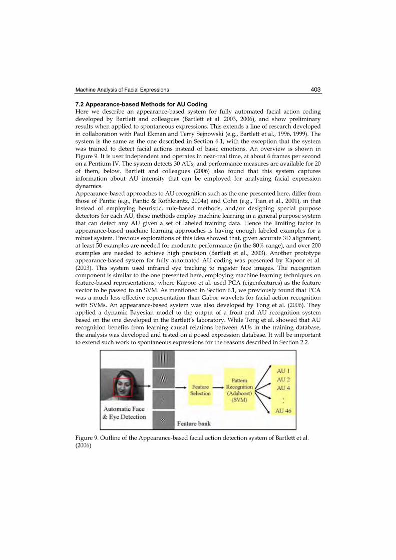
Machine Analysis of Facial Expressions 403
7.2 Appearance-based Methods for AU Coding
Here we describe an appearance-based system for fully automated facial action coding developed by Bartlett and colleagues (Bartlett et al. 2003, 2006), and show preliminary results when applied to spontaneous expressions. This extends a line of research developed in collaboration with Paul Ekman and Terry Sejnowski (e.g., Bartlett et al., 1996, 1999). The system is the same as the one described in Section 6.1, with the exception that the system was trained to detect facial actions instead of basic emotions. An overview is shown in Figure 9. It is user independent and operates in near-real time, at about 6 frames per second on a Pentium IV. The system detects 30 AUs, and performance measures are available for 20 of them, below. Bartlett and colleagues (2006) also found that this system captures information about AU intensity that can be employed for analyzing facial expression dynamics. Appearance-based approaches to AU recognition such as the one presented here, differ from those of Pantic (e.g., Pantic & Rothkrantz, 2004a) and Cohn (e.g., Tian et al., 2001), in that instead of employing heuristic, rule-based methods, and/or designing special purpose detectors for each AU, these methods employ machine learning in a general purpose system that can detect any AU given a set of labeled training data. Hence the limiting factor in appearance-based machine learning approaches is having enough labeled examples for a robust system. Previous explorations of this idea showed that, given accurate 3D alignment, at least 50 examples are needed for moderate performance (in the 80% range), and over 200 examples are needed to achieve high precision (Bartlett et al., 2003). Another prototype appearance-based system for fully automated AU coding was presented by Kapoor et al. (2003). This system used infrared eye tracking to register face images. The recognition component is similar to the one presented here, employing machine learning techniques on feature-based representations, where Kapoor et al. used PCA (eigenfeatures) as the feature vector to be passed to an SVM. As mentioned in Section 6.1, we previously found that PCA was a much less effective representation than Gabor wavelets for facial action recognition with SVMs. An appearance-based system was also developed by Tong et al. (2006). They applied a dynamic Bayesian model to the output of a front-end AU recognition system based on the one developed in the Bartlett’s laboratory. While Tong et al. showed that AU recognition benefits from learning causal relations between AUs in the training database, the analysis was developed and tested on a posed expression database. It will be important to extend such work to spontaneous expressions for the reasons described in Section 2.2.
Figure 9. Outline of the Appearance-based facial action detection system of Bartlett et al. (2006)

Face Recognition 404
Here we show performance of the system of Bartlett et al. (2006) for recognizing facial actions in posed and spontaneous expressions (Figure 10). The system was trained on both the Cohn-Kanade and Ekman-Hager datasets. The combined dataset contained 2568 training examples from 119 subjects. Performance presented here was for training and testing on 20 AUs. Separate binary classifiers, one for each AU, were trained to detect the presence of the AU regardless of the co-occurring AUs. Positive examples consisted of the last frame of each sequence which contained the expression apex. Negative examples consisted of all apex frames that did not contain the target AU plus neutral images obtained from the first frame of each sequence, for a total of 2568-N negative examples for each AU.
Figure 10. System performance (area under the ROC) for the AU detection system of Bartlett et al. (2006): (a) posed facial actions (sorted in order of detection performance), and (b) spontaneous facial actions (performance is overlayed on the posed results of (a); there were no spontaneous examples of AU 27 in this sample)

Machine Analysis of Facial Expressions 405
We first report performance for generalization to novel subjects within the Cohn-Kanade and Ekman-Hager databases. Generalization to new subjects was tested using leave-one-subject-out cross-validation in which all images of the test subject were excluded from training. The system obtained a mean of 91% agreement with human FACS labels. Overall percent correct can be an unreliable measure of performance, however, since it depends on the proportion of targets to non-targets, and also on the decision threshold. In this test, there was a far greater number of non-targets than targets, since targets were images containing the desired AU (N), and non-targets were all images not containing the desired AU (2568-N). A more reliable performance measure is area under the ROC (receiver-operator characteristic curve, or A’). This curve is obtained by plotting hit rate (true positives) against false alarm rate (false positives) as the decision threshold varies. A is equivalent to percent correct in a 2- alternative forced choice task, in which the system must choose which of two options contains the target on each trial. Mean A for the posed expressions was 92.6. A correlation analysis was performed in order to explicitly measure the relationship between the output margin and expression intensity. Ground truth for AU intensity was measured as follows: Five certified FACS coders labeled the action intensity for 108 images from the Ekman-Hager database, using the A-E scale of the FACS coding manual, where A is lowest, and E is highest. The images were four upper-face actions (1, 2, 4, 5) and two lower-face actions (10, 20), displayed by 6 subjects. We first measured the degree to which expert FACS coders agree with each other on intensity. Correlations were computed between intensity scores by each pair of experts, and the mean correlation was computed across all expert pairs. Correlations were computed separately for each display subject and each AU, and then means were computed across display subjects. Mean correlation between expert FACS coders within subject was 0.84.
Action unit 1 2 4 5 10 20 MeanExpert-Expert .92 .77 .85 .72 .88 .88 .84 SVM-Expert .90 .80 .84 .86 .79 .79 .83
Table 3. Correlation of SVM margin with intensity codes from human FACS experts
Correlations of the automated system with the human expert intensity scores were next computed. The SVMs were retrained on the even-numbered subjects of the Cohn-Kanade and Ekman-Hager datasets, and then tested on the odd-numbered subjects of the Ekman-Hager set, and vice versa. Correlations were computed between the SVM margin and the intensity ratings of each of the five expert coders. The results are shown in Table 3. Overall mean correlation between the SVM margin and the expert FACS coders was 0.83, which was nearly as high as the human-human correlation of .84. Similar findings were obtained using an AdaBoost classifier, where the AdaBoost output, which is the likelihood ratio of target/ nontarget, correlated positively with human FACS intensity scores (Bartlett et al., 2004). The system therefore is able to provide information about facial expression dynamics in terms of the frame-by-frame intensity information. This information can be exploited for deciding the presence of an AU and decoding the onset, apex, and offset. It will also enable studying the dynamics of facial behavior. As explained in section 2, enabling investigations into the dynamics of facial expression would allow researchers to directly address a number of questions key to understanding the nature of the human emotional and expressive systems, and their roles interpersonal interaction, development, and psychopathology.
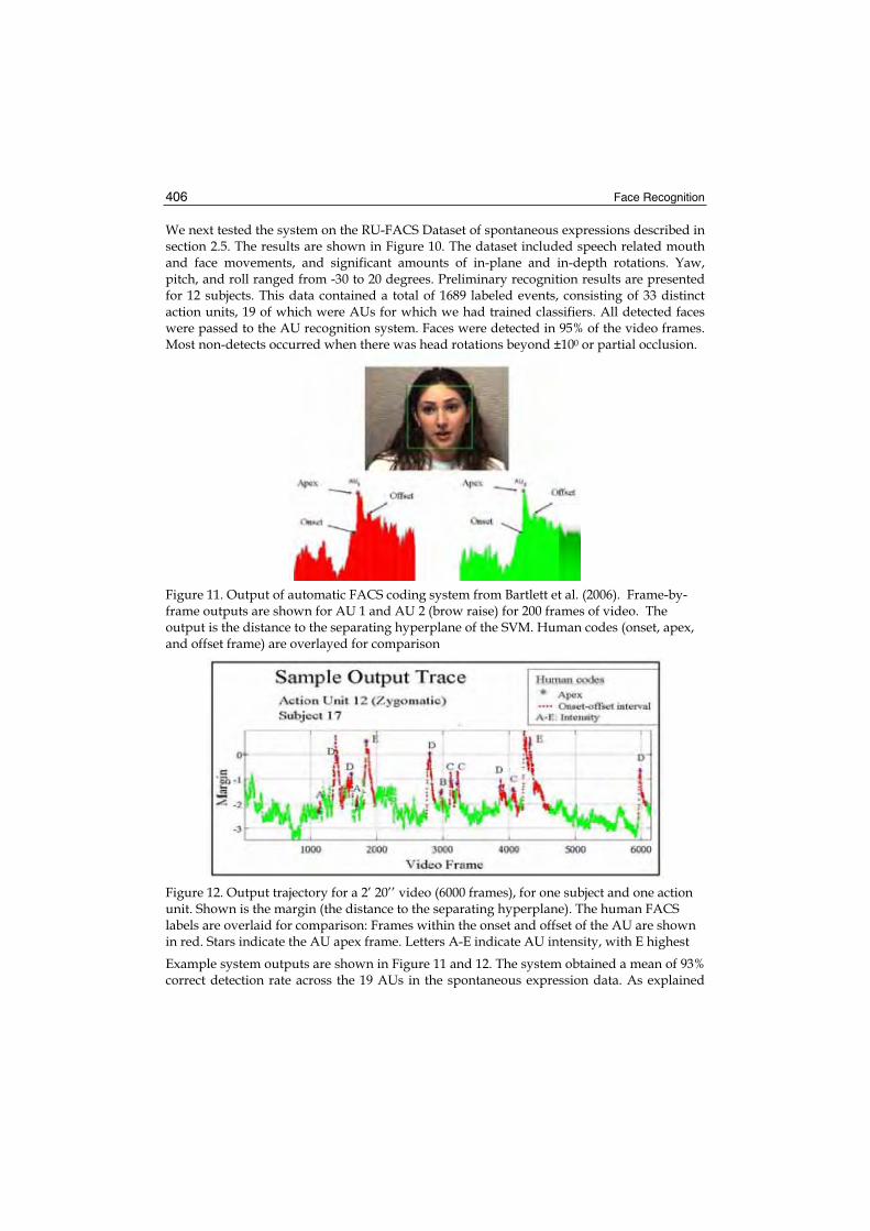
Face Recognition 406
We next tested the system on the RU-FACS Dataset of spontaneous expressions described in section 2.5. The results are shown in Figure 10. The dataset included speech related mouth and face movements, and significant amounts of in-plane and in-depth rotations. Yaw, pitch, and roll ranged from -30 to 20 degrees. Preliminary recognition results are presented for 12 subjects. This data contained a total of 1689 labeled events, consisting of 33 distinct action units, 19 of which were AUs for which we had trained classifiers. All detected faces were passed to the AU recognition system. Faces were detected in 95% of the video frames. Most non-detects occurred when there was head rotations beyond ±100 or partial occlusion.
Figure 11. Output of automatic FACS coding system from Bartlett et al. (2006). Frame-by-frame outputs are shown for AU 1 and AU 2 (brow raise) for 200 frames of video. The output is the distance to the separating hyperplane of the SVM. Human codes (onset, apex, and offset frame) are overlayed for comparison
Figure 12. Output trajectory for a 2’ 20’’ video (6000 frames), for one subject and one action unit. Shown is the margin (the distance to the separating hyperplane). The human FACS labels are overlaid for comparison: Frames within the onset and offset of the AU are shown in red. Stars indicate the AU apex frame. Letters A-E indicate AU intensity, with E highest
Example system outputs are shown in Figure 11 and 12. The system obtained a mean of 93% correct detection rate across the 19 AUs in the spontaneous expression data. As explained

Machine Analysis of Facial Expressions 407
above, however, percent correct can be misleading when there are unequal numbers of targets and nontargets. Mean area under the ROC for the spontaneous action units was .75 (and thus percent correct on a 2-alternative forced choice would be 75%). This figure is nevertheless encouraging, as it shows that fully automated systems can indeed get a signal about facial actions, despite generalizing from posed to spontaneous examples, and despite the presence of noise from speech and out-of-plane head rotations. As with the posed expression data, the SVM margin correlated positively with AU intensity in the spontaneous data (Figure 12). Mean correlation of AU 12 with FACS intensity score was .75, and the mean over eight AUs tested was 0.35.
7.3 Automatic Detection of Pain
The automated AU recognition system described above was applied to spontaneous facial expressions of pain (Littlewort et al., 2006b). The task was to differentiate faked from real pain expressions using the automated AU detector. Human subjects were videotaped while they submerged their hand in a bath of water for three minutes. Each subject experienced three experimental conditions: baseline, real pain, and posed pain. In the real pain condition, the water was 3 degrees Celsius, whereas in the baseline and posed pain conditions the water was 20 degrees Celsius. The video was coded for AUs by both human and computer. Our initial goal was to correctly determine which experimental condition is shown in a 60 second clip from a previously unseen subject. For this study, we trained individual AU classifiers on 3000 single frames selected from three datasets: two posed expression sets, the Cohn-Kanade and the Ekman-Hager datasets, and the RU-FACS dataset of spontaneous expression data. We trained linear SVM for each of 20 AUs, in one versus all mode, irrespective of combinations with other AUs. The output of the system was a real valued number indicating the distance to the separating hyperplane for each classifier. Applying this system to the pain video data produced a 20 channel output stream, consisting of one real value for each learned AU, for each frame of the video. This data was further analyzed to predict the difference between expressions of real pain and fake pain. The 20-channel output streams were passed to another set of three SVMs, trained to detect real pain, fake pain, and baseline. In a preliminary analysis of 5 subjects tested with cross-validation, the system correctly identified the experimental condition (posed pain, real pain, and baseline) for 93% of samples in a 3-way forced choice. The 2-way performance for fake versus real pain was 90%. This is considerably higher than the performance of naive human observers, who are near chance for identifying faked pain (Hadjistavropoulos et al., 1996).
8. Challenges, Opportunities and Recommendations
Automating the analysis of facial signals, especially rapid facial signals (facial expressions) is important to realize more natural, context-sensitive (e.g., affective) human-computer interaction, to advance studies on human emotion and affective computing, and to boost numerous applications in fields as diverse as security, medicine, and education. This chapter introduced recent advances in machine analysis of facial expressions and summarized the recent work of two forerunning research groups in this research field, namely that of Pantic and her colleagues and that of Bartlett and her colleagues. In summary, although most of the facial expression analyzers developed so far target human facial affect analysis and attempt to recognize a small set of prototypic emotional

Face Recognition 408
facial expressions like happiness and anger (Pantic et al., 2005a), some progress has been made in addressing a number of other scientific challenges that are considered essential for realization of machine understanding of human facial behavior. First of all, the research on automatic detection of facial muscle actions, which produce facial expressions, witnessed a significant progress in the past years. A number of promising prototype systems have been proposed recently that can recognize up to 27 AUs (from a total of 44 AUs) in either (near-) frontal view or profile view face image sequences (section 7 of this chapter; Tian et al. 2005). Further, although the vast majority of the past work in the field does not make an effort to explicitly analyze the properties of facial expression temporal dynamics, a few approaches to automatic segmentation of AU activation into temporal segments (neutral, onset, apex, offset) have been recently proposed (section 7 of this chapter). Also, even though most of the past work on automatic facial expression analysis is aimed at the analysis of posed (deliberately displayed) facial expressions, a few efforts were recently reported on machine analysis of spontaneous facial expressions (section 7 of this chapter; Cohn et al., 2004; Valstar et al., 2006; Bartlett et al., 2006). In addition, exceptions from the overall state of the art in the field include a few works towards detection of attitudinal and non-basic affective states such as attentiveness, fatigue, and pain (section 7 of this chapter; El Kaliouby & Robinson, 2004; Gu & Ji, 2004), a few works on context-sensitive (e.g., user-profiled) interpretation of facial expressions (Fasel et al., 2004; Pantic & Rothkrantz, 2004b), and an attempt to explicitly discern in an automatic way spontaneous from volitionally displayed facial behavior (Valstar et al., 2006). However, many research questions raised in section 2 of this chapter remain unanswered and a lot of research has yet to be done. When it comes to automatic AU detection, existing methods do not yet recognize the full range of facial behavior (i.e. all 44 AUs defined in FACS). For machine learning approaches, increasing the number of detected AUs boils down to obtaining labeled training data. To date, Bartlett’s team has means to detect 30 AUs, and do not yet have sufficient labeled data for the other AUs. In general, examples from over 50 subjects are needed. Regarding feature tracking approaches, a way to deal with this problem is to look at diverse facial features. Although it has been reported that methods based on geometric features are usually outperformed by those based on appearance features, recent studies like that of Pantic & Patras (2006), Valstar and Pantic (2006a), and those presented in this chapter, show that this claim does not always hold. We believe, however, that further research efforts toward combining both approaches are necessary if the full range of human facial behavior is to be coded in an automatic way. Existing methods for machine analysis of facial expressions discussed throughout this chapter assume that the input data are near frontal- or profile-view face image sequences showing facial displays that always begin with a neutral state. In reality, such assumption cannot be made. The discussed facial expression analyzers were tested on spontaneously occurring facial behavior, and do indeed extract information about facial behavior in less constrained conditions such as an interview setting (e.g., Bartlett et al., 2006; Valstar et al, 2006). However deployment of existing methods in fully unconstrained environments is still in the relatively distant future. Development of robust face detectors, head-, and facial feature trackers, which will be robust to variations in both face orientation relative to the camera, occlusions, and scene complexity like the presence of other people and dynamic background, forms the first step in the realization of facial expression analyzers capable of handling unconstrained environments.

Machine Analysis of Facial Expressions 409
Consequently, if we consider the state of the art in face detection and facial feature localization and tracking, noisy and partial data should be expected. As remarked by Pantic and Rothkrantz (2003), a facial expression analyzer should be able to deal with these imperfect data and to generate its conclusion so that the certainty associated with it varies with the certainty of face and facial point localization and tracking data. For example, the PFFL point tracker proposed by Patras and Pantic (2004, 2005) is very robust to noise, occlusion, clutter and changes in lighting conditions and it deals with inaccuracies in facial point tracking using a memory-based process that takes into account the dynamics of facial expressions. Nonetheless, this tracking scheme is not 100% accurate. Yet, the method proposed by Valstar and Pantic (2006a), which utilizes the PFFL point tracker, does not calculate the output data certainty by propagating the input data certainty (i.e., the certainty of facial point tracking). The only work in the field that addresses this issue is that of Pantic and Rothkrantz (2004a). It investigates AU recognition from static face images and explores the use of measures that can express the confidence in facial point localization and that can facilitate assessment of the certainty of the performed AU recognition. Another way of generating facial-expression-analysis output such that the certainty associated with it varies in accordance to the input data is to consider the time-instance versus time-scale dimension of facial behavior (Pantic & Rothkrantz, 2003). By considering previously observed data (time scale) with respect to the current data (time instance), a statistical prediction and its probability might be derived about both the information that may have been lost due to malfunctioning / inaccuracy of the camera (or a part of facial expression analyzer) and the currently displayed facial expression. Probabilistic graphical models, like Hidden Markov Models (HMM) and Dynamic Bayesian Networks (DBN) are well suited for accomplishing this (Pantic et al., 2005a). These models can handle noisy features, temporal information, and partial data by probabilistic inference. It remains unresolved, however, how the grammar of facial behavior can be learned (in a human-centered manner or in an activity-centered manner) and how this information can be properly represented and used to handle ambiguities in the observation data (Pantic et al., 2005a). Another related issue that should be addressed is how to include information about the context (environment, user, user’s task) in which the observed expressive behavior was displayed so that a context-sensitive analysis of facial behavior can be achieved. These aspects of machine analysis of facial expressions form the main focus of the current and future research in the field. Yet, since the complexity of these issues concerned with the interpretation of human behavior at a deeper level is tremendous and spans several different disciplines in computer and social sciences, we believe that a large, focused, interdisciplinary, international program directed towards computer understanding of human behavioral patterns (as shown by means of facial expressions and other modes of social interaction) should be established if we are to experience true breakthroughs in this and the related research fields.
9. References
Ambadar, Z., Schooler, J. & Cohn, J.F. (2005). Deciphering the enigmatic face: The importance of facial dynamics in interpreting subtle facial expressions. Psychological Science, Vol. 16, No. 5, pp. 403-410.

Face Recognition 410
Ambady, N. & Rosenthal, R. (1992). Thin Slices of Expressive Behavior as Predictors of Interpersonal Consequences: A Meta-Analysis. Psychological Bulletin, Vol. 111, No. 2, pp. 256-274.
Anderson, K. & McOwan, P.W. (2006). A Real-Time Automated System for Recognition of Human Facial Expressions. IEEE Trans. Systems, Man, and Cybernetics – Part B, Vol. 36, No. 1, pp. 96-105.
Barron, J., Fleet, D. & Beauchemin, S. (1994). Performance of optical flow techniques. J. Computer Vision, Vol. 12, No. 1, pp. 43-78.
Bartlett, M.S., Hager, J. C., Ekman, P. & Sejnowski, T.J. (1999). Measuring facial expressions by computer image analysis. Psychophysiology, Vol. 36, No. 2, pp. 253-263.
Bartlett, M.S., Littlewort, G., Braathen, B., Sejnowski, T.J., & Movellan, J.R. (2003a). A prototype for automatic recognition of spontaneous facial actions. Advances in Neural Information Processing Systems, Vol. 15, pp. 1271-1278.
Bartlett, M.S., Littlewort, G., Fasel, I. & Movellan, J.R. (2003b). Real time face detection and expression recognition: Development and application to human-computer interaction, Proc. CVPR Workshop on Computer Vision and Pattern Recognition for Human-Computer Interaction, p. 6.
Bartlett, M.S., Littlewort, G., Frank, M.G., Lainscsek, C., Fasel, I. & Movellan, J. (2005). Recognizing facial expression: machine learning and application to spontaneous behavior, Proc. IEEE Int’l Conf. Computer Vision and Pattern Recognition, pp. 568-573.
Bartlett, M.S., Littlewort, G., Frank, M.G., Lainscsek, C., Fasel, I. & Movellan, J. (2006). Fully automatic facial action recognition in spontaneous behavior, Proc. IEEE Conf. Automatic Face & Gesture Recognition, pp. 223-230.
Bartlett, M., Littlewort, G., Lainscsek, C., Fasel, I. & Movellan, J. (2004). Machine learning methods for fully automatic recognition of facial expressions and facial actions, Proc. IEEE Int’l Conf. Systems, Man and Cybernetics, Vol. 1, pp. 592-597.
Bartlett, M.S., Viola, P.A., Sejnowski, T.J., Golomb, B.A., Larsen, J., Hager, J.C. & Ekman, P. (1996). Classifying facial actions, Advances in Neural Information Processing Systems 8,pp. 823-829.
Bassili, J.N. (1978). Facial motion in the perception of faces and of emotional expression. J. Experimental Psychology, Vol. 4, No. 3, pp. 373-379.
Black, M. & Yacoob, Y. (1997). Recognizing facial expressions in image sequences using local parameterized models of image motion. Computer Vision, Vol. 25, No. 1, pp. 23-48.
Bowyer, K.W. (2004). Face Recognition Technology – Security vs. Privacy. IEEE Technology and Society Magazine, Vol. 23, No. 1, pp. 9-19.
Brodal, A. (1981). Neurological anatomy: In relation to clinical medicine. Oxford University Press, New York, USA.
Chang, Y., Hu, C., Feris, R. & Turk, M. (2006). Manifold based analysis of facial expression. J.Image & Vision Computing, Vol. 24, No. 6, pp. 605-614.
Chen, L., Zhang, L., Zhang, H. & Abdel-Mottaleb, M. (2004). 3D Shape Constraint for Facial Feature Localization using Probabilistic-like Output, Proc. IEEE Int'l Workshop Analysis and Modeling of Faces and Gestures, pp. 302-307.
Cohen, I., Sebe, N., Garg, A., Chen, L.S. & Huang, T.S. (2003). Facial expression recognition from video sequences – temporal and static modelling. Computer Vision and Image Understanding, Vol. 91, pp. 160-187.
Cohen, M.M. (2006). Perspectives on the Face, Oxford University Press, Oxford, UK:

Machine Analysis of Facial Expressions 411
Cohn, J.F. (2006). Foundations of human computing: Facial expression and emotion, Proc.ACM Int’l Conf. Multimodal Interfaces, pp. 233-238.
Cohn, J.F. & Ekman, P. (2005). Measuring facial actions, In: The New Handbook of Methods in Nonverbal Behavior Research, Harrigan, J.A., Rosenthal, R. & Scherer, K., (Eds.), pp. 9-64, Oxford University Press, New York, USA.
Cohn, J.F., Reed, L.I., Ambadar, Z., Xiao, J. and Moriyama, T. (2004). Automatic analysis and recognition of brow actions in spontaneous facial behavior, Proc. IEEE Int’l Conf. Systems, Man & Cybernetics, pp. 610-616.
Cohn, J.F. & Schmidt, K.L. (2004). The timing of facial motion in posed and spontaneous smiles. J. Wavelets, Multi-resolution & Information Processing, Vol. 2, No. 2, pp. 121-132.
Costa, M., Dinsbach, W., Manstead, A.S.R. & Bitti P.E.R. (2001). Social presence, embarrassment, and nonverbal behaviour. J. Bonverbal Behaviour, Vol. 25., No. 4, pp. 225-240.
Craig, K., Hyde, S.A. & Patrick, C.J. (1991). Genuine, suppressed, and faked facial behavior during exacerbation of chronic low back pain. Pain, Vol. 46, pp. 161–172.
Cunningham, D.W., Kleiner, M., Wallraven, C. & Bülthoff, H.H. (2004). The components of conversational facial expressions, Proc. ACM Int’l Symposium on Applied Perception in Graphics and Visualization, pp. 143-149.
Darwin, C. (1872/1998). The expression of the emotions in man and animals, Oxford University Press, New York, USA.
Daugman, J. (1988). Complete discrete 2D Gabor transform by neural networks for image analysis and compression. IEEE Trans. Acoustics, Speech, and Signal Processing, Vol. 36, pp. 1169-1179.
DeCarlo, D. & Metaxas, D. (1996). The integration of optical flow and deformable models with applications to human face shape and motion estimation, Proc. IEEE Int’l Conf. Computer Vision and Pattern Recognition, pp. 231-238.
Donato, G., Bartlett, M.S., Hager, J.C., Ekman, P. & Sejnowski, T.J. (1999). Classifying facial actions. IEEE Trans. Pattern Analysis and Machine Intelligence, Vol. 21, No. 10, pp. 974-989.
Duchenne de Bologne, G.B. (1862/1990). Mechanisme de la Physionomie Humaine, Jules Renouard Libraire, Paris, France, 1862. (Translation: The Mechanism of Human Facial Expression, Cambridge University Press, New York, USA, 1990).
Edwards, G.J., Cootes, T.F. & Taylor, C.J. (1998). Face Recognition Using Active Appearance Models, Proc. European Conf. Computer Vision, Vol. 2, pp. 581-695.
Ekman, P. (1991). Telling Lies: Clues to Deceit in the Marketplace, Politics, and Marriage. W.W. Norton, New York, USA.
Ekman, P. (2003). Darwin, deception, and facial expression. Annals New York Academy of sciences, Vol. 1000, pp. 205-221.
Ekman, P. (1989). The argument and evidence about universals in facial expressions of emotion. In: Psychological methods in criminal investigation and evidence, Raskin, D.C., (Ed.), pp. 297–332, Springer, New York, USA.
Ekman, P. & Friesen, W.V. (1969). The repertoire of nonverbal behavior. Semiotica, Vol. 1, pp. 49-98.
Ekman, P. & Friesen, W.V. (1975). Unmasking the face, Prentice-Hall, New Jersey, USA.

Face Recognition 412
Ekman, P. & Friesen, W.V. (1978). Facial Action Coding System, Consulting Psychologist Press, Palo Alto, USA.
Ekman, P., Friesen, W.V. & Hager, J.C. (2002). Facial Action Coding System, A Human Face, Salt Lake City, USA.
Ekman, P., Hager, J.C., Methvin, C.H. & Irwin, W. (1999). Ekman-Hager Facial Action Exemplars (unpublished), Human Interaction Lab, University of California, San Francisco, USA.
Ekman, P., Huang, T.S., Sejnowski, T.J. & Hager, J.C., (Eds.), (1993). NSF Understanding the Face, A Human Face eStore, Salt Lake City, USA, (see Library).
Ekman, P. & Rosenberg, E.L., (Eds.), (2005). What the face reveals: Basic and applied studies of spontaneous expression using the FACS, Oxford University Press, Oxford, UK.
El Kaliouby, R. & Robinson, P. (2004). Real-Time Inference of Complex Mental States from Facial Expressions and Head Gestures, Proc. IEEE Int’l Conf. Computer Vision and Pattern Recognition, Vol. 3, p. 154.
Essa, I. & Pentland, A. (1997). Coding, analysis, interpretation, and recognition of facial expressions. IEEE Trans. Pattern Analysis and Machine Intelligence, Vol. 19, No. 7, pp. 757-763.
Fasel, B., Monay, F. & Gatica-Perez, D. (2004). Latent semantic analysis of facial action codes for automatic facial expression recognition, Proc. ACM Int’l Workshop on Multimedia Information Retrieval, pp. 181-188.
Fasel, I.R. (2006). Learning Real-Time Object Detectors: Probabilistic Generative Approaches. PhD thesis, Department of Cognitive Science, University of California, San Diego, USA.
Fasel, I.R., Fortenberry, B. & Movellan, J.R. (2005). A generative framework for real time object detection and classification. Int'l J Computer Vision and Image Understanding,Vol. 98, No. 1, pp. 181-210.
Frank, M.G. & Ekman, P. (2004). Appearing truthful generalizes across different deception situations. Journal of personality and social psychology, Vol. 86, pp. 486–495.
Friedman, J., Hastie, T. & Tibshirani, R. (2000). Additive logistic regression: a statistical view of boosting. The Annals of Statistics, Vol. 28, No 2, pp. 337-374.
Gokturk, S.B., Bouguet, J.Y., Tomasi, C. & Girod, B. (2002). Model-based face tracking for view independent facial expression recognition, Proc. IEEE Int’l Conf. Face and Gesture Recognition, pp. 272-278.
Gross, R., Matthews, I. & Baker, S. (2006). Active appearance models with occlusion. J. Image & Vision Computing, Vol. 24, No. 6, pp. 593-604.
Gu, H. & Ji, Q. (2004). An automated face reader for fatigue detection, Proc. IEEE Int’l Conf. Face and Gesture Recognition, pp. 111-116.
Gu, H. & Ji, Q. (2005). Information extraction from image sequences of real-world facial expressions. Machine Vision and Applications, Vol. 16, No. 2, pp. 105-115.
Guo, G. & Dyer, C.R. (2005). Learning From Examples in the Small Sample Case – Face Expression Recognition. IEEE Trans. Systems, Man, and Cybernetics – Part B, Vol. 35, No. 3, pp. 477-488.
Hadjistavropoulos, H.D., Craig, K.D., Hadjistavropoulos, T. & Poole, G.D. (1996). Subjective judgments of deception in pain expression: Accuracy and errors. Pain, Vol. 65, pp. 247-254.
Haykin, S. & de Freitas, N., (Eds.), (2004). Special Issue on Sequential State Estimation. Proceedings of the IEEE, vol. 92, No. 3, pp. 399-574.

Machine Analysis of Facial Expressions 413
Heller, M. & Haynal, V. (1997). Depression and suicide faces. In: What the Face Reveals,Ekman, P. & Rosenberg, E., (Eds.), pp. 339-407, Oxford University Press, New York, USA.
Hess, U., Blairy, S. & Kleck, R.E. (1997). The intensity of emotional facial expressions and decoding accuracy. J. Nonverbal Behaviour, Vol. 21, No. 4, pp. 241-257.
Holden, E. & Owens, R. (2002). Automatic Facial Point Detection, Proc. Asian Conf. Computer Vision, vol. 2, pp 731-736.
Huang, K.S. & Trivedi, M.M. (2004). Robust Real-Time Detection, Tracking, and Pose Estimation of Faces in Video Streams, Proc. IEEE Int’l Conf. Pattern Recognition, Vol. 3, pp. 965-968.
Humphreys, G.W., Donnelly, N. & Riddoch, M.J. (1993). Expression is computed separately from facial identity and it is computed separately for moving and static faces – Neuropsychological evidence. Neuropsychologia, Vol. 31, pp. 173-181.
Isard, M. & Blake, A. (1998). Condensation - conditional density propagation for visual tracking. J. Computer Vision, Vol. 29, No. 1, pp. 5-28.
Kalman, R.E. (1960). A new approach to linear filtering and prediction problems. Trans. ASME J. Basic Eng., Vol. 82, pp. 35-45.
Kanade, T., Cohn, J.F. & Tian, Y. (2000). Comprehensive database for facial expression analysis, Proc. IEEE Int’l Conf. Face and Gesture Recognition, pp. 46-53.
Kapoor, A., Qi Y. & Picard, R.W. (2003). Fully automatic upper facial action recognition, Proc. IEEE Int’l Workshop on Analysis and Modeling of Faces and Gestures, pp. 195-202.
Keltner, D. (1997). Signs of Appeasement: Evidence for distinct displays of embarrassment, amusement, and shame, In: What the Face Reveals, Ekman, P. & Rosenberg, E., (Eds.), pp. 133-160, Oxford University Press, New York, USA.
Keltner, D. & Ekman, P. (2000). Facial Expression of Emotion, In: Handbook of Emotions, Lewis, M. & Haviland-Jones, J.M., (Eds.), pp. 236-249, Guilford Press, New York, USA.
Kimura, S. & Yachida, M. (1997). Facial expression recognition and its degree estimation, Proc. IEEE Int’l Conf. Computer Vision and Pattern Recognition, pp. 295-300.
Lades, M., Vorbruggen, J.C., Buhmann, J., Lange, J., von der Malsburg, C., Wurtz, R.P. & Konen, W. (1992). Distortion Invariant Object Recognition in the Dynamik Link Architecture. IEEE Transactions on Computers, Vol. 42, No. 3, pp. 300-311.
Li, S.Z. & Jain, A.K., (Eds.), (2005). Handbook of Face Recognition, Springer, New York, USA. Lien, J.J.J., Kanade, T., Cohn, J.F. & Li, C.C. (1998). Subtly different facial expression
recognition and expression intensity estimation, Proc. IEEE Int’l Conf. Computer Vision and Pattern Recognition, pp. 853-859.
Littlewort, G., Bartlett, M.S., Fasel, I., Susskind, J. & Movellan, J. (2006). Dynamics of facial expression extracted automatically from video. J. Image & Vision Computing, Vol. 24, No. 6, pp. 615-625.
Littlewort, G., Bartlett, M.S. & Lee, K. (2006b). Faces of Pain: Automated measurement of spontaneous facial expressions of genuine and posed pain, Proc. 13th Joint Symposium on Neural Computation, p. 1.
Lucas, B.D. & Kanade, T. (1981). An iterative image registration technique with an application to stereo vision, Proc. Conf. Artificial Intelligence, pp. 674-679.
Lyons, M.J.; Budynek, J. &Akamatsu, S. (1999). Automatic classification of single facial images. IEEE Trans. Pattern Analysis and Machine Intelligence, Vol. 21, No. 12, pp. 1357-1362.

Face Recognition 414
Maat, L. & Pantic, M. (2006). Gaze-X: Adaptive affective multimodal interface for single-user office scenarios, Proc. ACM Int’l Conf. Multimodal Interfaces, pp. 171-178.
Martinez, A. M. (2003). Matching expression variant faces. Vision Research, Vol. 43, No. 9, pp. 1047-1060.
Mase, K. (1991). Recognition of facial expression from optical flow. IEICE Transactions, Vol. E74, No. 10, pp. 3474-3483.
Meihlke, A. (1973). Surgery of the facial nerve. Saunders, Philadelphia, USA. Moghaddam, B. & Pentland, A. (1997). Probabilistic Visual Learning for Object Recognition.
IEEE Trans. Pattern Analysis and Machine Intelligence, Vol. 19, No. 7, pp. 696-710. Nock, H.J., Iyengar, G. & Neti, C. (2004). Multimodal processing by finding common cause.
Communications of the ACM, Vol. 47, No. 1, pp. 51-56. O’Toole, A.J., Harms, J., Snow, S.L., Hurst, D.R., Pappas, M.R., Ayyad, J.H. & Abdi, H.
(2005). A video database of moving faces and people. IEEE Transactions on Pattern Analysis and Machine, Vol. 27, No. 5, pp. 812–816.
Osadchy, M., Jacobs, D.W. & Lindenbaum, M. (2005). On the equivalence of common approaches to lighting insensitive recognition, Proc. IEEE Int’l Conf. Computer Vision, pp. 1721-1726.
Pantic, M. (2006). Face for Ambient Interface. Lecture Notes in Artificial Intelligence, vol. 3864, pp. 35-66.
Pantic, M. & Patras, I. (2005). Detecting facial actions and their temporal segments in nearly frontal-view face image sequences, Proc. IEEE Int'l Conf. on Systems, Man and Cybernetics, pp. 3358-3363.
Pantic, M. & Patras, I. (2006). Dynamics of facial expression: Recognition of facial actions and their temporal segments from face profile image sequences. IEEE Trans. on Systems, Man and Cybernetics - Part B, Vol. 36, No. 2, pp. 433-449.
Pantic, M., Pentland, A., Nijholt, A. & Huang, T. (2006). Human Computing and machine understanding of human behaviour: A Survey, Proc. ACM Int’l Conf. Multimodal Interfaces, pp. 239-248.
Pantic, M. & Rothkrantz, L.J.M. (2000). Automatic Analysis of Facial Expressions – The State of the Art. IEEE Trans. Pattern Analysis and Machine Intelligence, Vol. 22, No. 12, pp. 1424-1445.
Pantic, M. & Rothkrantz, L.J.M. (2003). Toward an Affect-Sensitive Multimodal Human-Computer Interaction. Proceedings of the IEEE, Spec. Issue on Human-Computer Multimodal Interface, Vol. 91, No. 9, pp. 1370-1390.
Pantic, M. & Rothkrantz, L.J.M. (2004a). Facial action recognition for facial expression analysis from static face images. IEEE Trans. on Systems, Man and Cybernetics - Part B, Vol. 34, No. 3, pp. 1449-1461.
Pantic, M. & Rothkrantz, L.J.M. (2004b). Case-based reasoning for user-profiled recognition of emotions from face images, Proc. IEEE Int’l Conf. Multimedia & Expo, pp. 391-394.
Pantic, M., Rothkrantz, L.J.M. & Koppelaar, H. (1998). Automation of non-verbal communication of facial expressions, Proc. Conf. Euromedia, pp. 86-93.
Pantic, M., Sebe, N., Cohn, J.F. & Huang, T. (2005a). Affective Multimodal Human-Computer Interaction, Proc. ACM Int'l Conf. on Multimedia, pp. 669-676.
Pantic, M., Valstar, M.F., Rademaker, R. & Maat, L. (2005b). Web-based database for facial expression analysis, Proc. IEEE Int’l Conf. Multimedia and Expo, pp. 317-321. (www.mmifacedb.com)

Machine Analysis of Facial Expressions 415
Patras, I. & Pantic, M. (2004). Particle filtering with factorized likelihoods for tracking facial features, Proc. IEEE Int'l Conf. Face and Gesture Recognition, pp. 97-102.
Patras, I. & Pantic, M. (2005). Tracking deformable motion, Proc. IEEE Int'l Conf. on Systems, Man and Cybernetics, pp. 1066-1071.
Pentland, A., Moghaddam, B. & Starner, T. (1994). View-Based and Modular Eigenspaces for Face Recognition, Proc. Conf. Computer Vision and Pattern Recognition, pp. 84-91.
Picard, R.W. (1997). Affective Computing, MIT Press, Cambridge, USA. Pitt, M.K. & Shephard, N. (1999). Filtering via simulation: auxiliary particle filtering. J. Amer.
Stat. Assoc., Vol. 94, pp. 590-599. Rinn, W. E. (1984). The neuropsychology of facial expression: A review of the neurological
and psychological mechanisms for producing facial expressions. Psychological Bulletin, Vol. 95, No. 1, pp. 52–77.
Roark, D.A., Barret, S.E., Spence, M.J., Abdi, H. & O’Toole, A.J. (2003). Psychological and neural perspectives on the role of motion in face recognition. Behavioral and cognitive neuroscience reviews, Vol. 2, No. 1, pp. 15-46.
Rowley, H., Baluja, S. & Kanade, T. (1998). Neural Network-Based Face Detection. IEEE Trans. Pattern Analysis and Machine Intelligence, Vol. 20, No. 1, pp. 23-38.
Russell, J.A. & Fernandez-Dols, J.M., (Eds.), (1997). The Pshychology of Facial Expression,Cambridge University Press, New York, USA.
Samal, A. & Iyengar, P.A. (1992). Automatic recognition and analysis of human faces and facial expressions: A survey. Pattern Recognition, Vol. 25, No. 1, pp. 65-77.
Sayette, M.A., Smith, D.W., Breiner, M.J. & Wilson, G.T. (1992). The effect of alcohol on emotional response to a social stressor. Journal of Studies on Alcohol, Vol. 53, pp. 541–545.
Scherer, K.R. & Ekman, P., (Eds.), (1982). Handbook of methods in non-verbal behavior research.Cambridge University Press, Cambridge, USA.
Schneiderman, H. & Kanade, T. (2000). A statistical model for 3D object detection applied to faces and cars, Proc. Conf. Computer Vision and Pattern Recognition, pp. 746-751.
Shi, J. & Tomasi, C. (1994). Good features to track, Proc. IEEE Int’l Conf. Computer Vision and Pattern Recognition, pp. 593-600.
Su, C., Zhuang, Y., Huang, L. & Wu, F. (2004). A Two-Step Approach to Multiple Facial Feature Tracking: Temporal Particle Filter and Spatial Belief Propagation, Proc. IEEE Int'l Conf. Face and Gesture Recognition, pp. 433-438.
Sung, K.K. & Poggio, T. (1998). Example-Based Learning for View-Based Human Face Detection. IEEE Trans. Pattern Analysis and Machine Intelligence, Vol. 20, No. 1, pp. 39-51.
Tao, H. & Huang, T.S. (1998). Connected vibrations – a model analysis approach to non-rigid motion tracking, Proc. IEEE Int’l Conf. Computer Vision and Pattern Recognition,pp. 735-740.
Tian, Y.L., Kanade, T. & Cohn, J.F. (2001). Recognizing action units for facial expression analysis. IEEE Trans. Pattern Analysis and Machine Intelligence, Vol. 23, No. 2, pp. 97-115.
Tian, Y.L., Kanade, T. & Cohn, J.F. (2005). Facial Expression Analysis, In: Handbook of Face Recognition, Li, S.Z. & Jain, A.K., (Eds.), pp. 247-276, Springer, New York, USA.
Tong, Y., Liao, W. & Ji, Q. (2006). Inferring facial action units with causal relations, Proc. IEEE Int’l Conf. Computer Vision and Pattern Recognition, pp. 1623-1630.

Face Recognition 416
Torres, E. & Andersen, R. (2006). Space-time separation during obstacle-avoidance learning in monkeys. J. Neurophysiology, Vol. 96, pp. 2613-2632.
Valstar, M.F. & Pantic, M. (2006a). Fully automatic facial action unit detection and temporal analysis, Proc. IEEE Int’l Conf. Computer Vision and Pattern Recognition, Vol. 3, p. 149.
Valstar, M.F. & Pantic, M. (2006b). Biologically vs. logic inspired encoding of facial actions and emotions in video, Proc. IEEE Int'l Conf. Multimedia and Expo.
Valstar, M.F., Pantic, M., Ambadar, Z. & Cohn, J.F. (2006). Spontaneous vs. posed facial behavior: Automatic analysis of brow actions, Proc. ACM Int'l Conf. Multimodal Interfaces, pp. 162-170.
Valstar, M., Pantic, M. & Patras, I. (2004). Motion History for Facial Action Detection from Face Video, Proc. IEEE Int’l Conf. Systems, Man and Cybernetics, Vol. 1, pp. 635-640.
Viola, P. & Jones, M. (2004). Robust real-time face detection. J. Computer Vision, Vol. 57, No. 2, pp. 137-154.
Vukadinovic, D. & Pantic, M. (2005). Fully automatic facial feature point detection using Gabor feature based boosted classifiers, Proc. IEEE Int'l Conf. Systems, Man and Cybernetics, pp. 1692-1698.
Wang, P. & Ji, Q. (2004). Multi-View Face Detection under Complex Scene based on Combined SVMs, Proc. IEEE Int’l Conf. Pattern Recognition, Vol. 4, pp. 179-182.
Williams, A.C. (2002). Facial expression of pain: An evolutionary account. Behavioral & Brain Sciences, Vol. 25, No. 4, pp. 439-488.
Whitehill, J. & Omlin, C. 2006). Haar Features for FACS AU Recognition, Proc. IEEE Int’l Conf. Face and Gesture Recognition, 5 pp.
Xiao, J., Baker, S., Matthews, I. & Kanade, T. (2004). Real-time Combined 2D+3D Active Appearance Models, Proc. IEEE Int’l Conf. Computer Vision and Pattern Recognition,pp. 535-542.
Xiao, J., Moriyama, T., Kanade, T. & Cohn, J.F. (2003). Robust full-motion recovery of head by dynamic templates and re-registration techniques. Int’l J. Imaging Systems and Technology, Vol. 13, No. 1, pp. 85-94.
Yacoob, Y., Davis, L., Black, M., Gavrila, D., Horprasert, T. & Morimoto, C. (1998). Looking at People in Action, In: Computer Vision for Human-Machine Interaction, Cipolla, R. & Pentland, A., (Eds.), pp. 171-187, Cambridge University Press, Cambridge, UK.
Yang, M.H., Kriegman, D.J. & Ahuja, N. (2002). Detecting faces in images: A survey. IEEE Trans. Pattern Analysis and Machine Intelligence, Vol. 24, No. 1, pp. 34-58.
Yin, L., Wei, X., Sun, Y., Wang, J. & Rosato, M. (2006). A 3d facial expression database for facial behavior research, Proc. IEEE Int’l Conf. Face and Gesture Recognition, pp. 211-216.
Young, A.W., (Ed.), (1998). Face and Mind, Oxford University Press, Oxford, UK. Zhang, Y. & Ji, Q. (2005). Active and dynamic information fusion for facial expression
understanding from image sequence. IEEE Trans. Pattern Analysis & Machine Intelligence, Vol. 27, No. 5, pp. 699-714.
Zhang, Z., Lyons, M., Schuster, M. & Akamatsu, S. (1998). Comparison Between Geometry-based and Garbor-Wavelet- based Facial Expression Recognition Using Multi-layer Perceptron, Proc. IEEE Int’l Conf. Face and Gesture Recognition, pp. 454-459.
Zhao, W., Chellappa, R., Rosenfeld, A. & Phillips, P.J. (2003). Face Recognition – A literature survey. ACM Computing Surveys, Vol. 35, No. 4, pp. 399-458.
21
3D Face Recognition
Theodoros Papatheodorou and Daniel Rueckert Department of Computing, Imperial College London
UK
1. Introduction
The survival of an individual in a socially complex world depends greatly on the ability to interpret visual information about the age, sex, race, identity and emotional state of another person based on that person’s face. Despite a variety of different adverse conditions (varying facial expressions and facial poses, differences in illumination and appearance), humans can perform face identification with remarkable robustness without conscious effort.Face recognition research using automatic or semi-automatic techniques emerged in the 1960s, and especially in the last two decades it has received significant attention. One reason for this growing interest is the wide range of possible applications for face recognition systems. Another reason is the emergence of affordable hardware, such as digital photography and video, which have made the acquisition of high-quality and high-resolution images much more ubiquitous. Despite this growing attention, the current state-of-the-art face recognition systems perform well when facial images are captured under uniform and controlled conditions. However, the development of face recognition systems that work robustly in uncontrolled situations is still an open research issue. Even though there are various alternative biometric techniques that perform very well today, e.g. fingerprint analysis and iris scans, these methods require the cooperation of the subjects and follow a relatively strict data acquisition protocol. Face recognition is much more flexible since subjects are not necessarily required to cooperate or even be aware of being scanned and identified. This makes face recognition a less intrusive and potentially more effective identification technique. Finally, the public’s perception of the face as a biometric modality is more positive compared to the other modalities (Hietmeyer, 2000).
1.1 Challenges for face recognition
The face is a three-dimensional (3D) object. Its appearance is determined by the shape as well as texture of the face. Broadly speaking, the obstacles that a face recognition systemmust overcome are differences in appearance due to variations in illumination, viewing angle, facial expressions, occlusion and changes over time. Using 2D images for face recognition, the intensities or colours of pixels represent all the information that is available and therefore, any algorithm needs to cope with variation due to illumination explicitly. The human brain seems also to be affected by illumination in performing face recognition tasks (Hill et al., 1997). This is underlined by the difficulty of identifying familiar faces when lit from above (Johnston et al., 1992) or from different

Face Recognition 418
directions (Hill and Bruce, 1996). Similarly it has been shown that faces shown in photographic negatives had a detrimental effect on the identification of familiar faces (Bruce and Langton, 1994). Further studies have shown that the effect of lighting direction can be a determinant of the photographic negative effect (Liu et al., 1999). As a result, positive faces, which normally appear to be top-lit, may be difficult to recognize in negative partly because of the accompanying change in apparent lighting direction to bottom-lit. One explanation for these findings is that dramatic illumination or pigmentation changes interfere with the shape-from-shading processes involved in constructing representations of faces. If the brain reconstructs 3D shape from 2D images, it remains a question why face recognition by humans remains viewpointdependent to the extent it is. One of the key challenges for face recognition is the fact that the difference between two images of the same subject photographed from different angles is greater than the differences between two images of different subjects photographed from the same angle. It has been reported that recognition rates for unfamiliar faces drop significantly when there are different viewpoints for the training and test set (Bruce, 1982). More recently, however, there has been debate about whether object recognition is viewpoint-dependent or not (Tarr and Bulthoff, 1995). It seems that the brain is good at generalizing from one viewpoint to another as long as the change in angle is not extreme. For example, matching a profile viewpoint to a frontal image is difficult, although the matching of a three-quarter view to a frontal seems to be less difficult (Hill et al., 1997). There have been suggestions that the brain might be storing a view-specific prototype abstraction of a face in order to deal with varying views (Bruce, 1994). Interpolation-based models (Poggio and Edelman, 1991), for example, support the idea that the brain identifies faces across different views by interpolating to the closest previously seen view of the face. Another key challenge for face recognition is the effect of facial expressions on the appearance of the face. The face is a dynamic structure that changes its shape non-rigidly since muscles deform soft tissue and move bones. Neurophysiologic studies have suggested that facial expression recognition happens in parallel to face identification (Bruce, 1988). Some case studies in prosopagnostic patients show that they are able to recognize expressions even though identifying the actor remains a near-impossible task. Similarly, patients who suffer from organic brain syndrome perform very poorly in analyzing expressions but have no problems in performing face recognition. However, the appearance of the face also changes due to aging and people’s different lifestyles. For example, skin becomes less elastic and more loose with age, the lip and hair-line often recedes, the skin color changes, people gain or lose weight, grow a beard, change hairstyle etc. This can lead to dramatic changes in the appearance of faces in images. A final challenge for face recognition is related to the problem of occlusions. Such occlusions can happen for a number of reasons, e.g. part of the face maybe occluded and not visiblewhen images are taken from certain angles or because the subject grew a beard, is wearing glasses or a hat.
2. From 2D to 3D face recognition
2D face recognition is a much older research area than 3D face recognition research and broadly speaking, at the present, the former still outperforms the latter. However, the wealth of information available in 3D face data means that 3D face recognition techniques

3D Face Recognition 419
might in the near future overtake 2D techniques. In the following we examine some of the inherent differences between 2D and 3D face recognition.
2.1 Advantages and disadvantages of 3D face recognition
As previously discussed, face recognition using 2D images is sensitive to illumination changes. The light collected froma face is a function of the geometry of the face, the albedo of the face, the properties of the light source and the properties of the camera. Given this complexity, it is difficult to develop models that take all these variations into account. Training using different illumination scenarios as well as illumination normalization of 2D images has been used, but with limited success. In 3D images, variations in illumination only affect the texture of the face, yet the captured facial shape remains intact (Hesher et al., 2003).Another differentiating factor between 2D and 3D face recognition is the effect of pose variation. In 2D images effort has been put into transforming an image into a canonical position (Kim and Kittler, 2005). However, this relies on accurate landmark placement and does not tackle the issue of occlusion. Moreover, in 2D this task is nearly impossible due to the projective nature of 2D images. To circumvent this problem it is possible to store different views of the face (Li et al., 2000). This, however, requires a large number of 2D images from many different views to be collected. An alternative approach to address the pose variation problem in 2D images is either based on statistical models for view interpolation (Lanitis et al., 1995; Cootes et al., 1998) or on the use of generative models (Prince and Elder, 2006). Other strategies including sampling the plenoptic function of a face using lightfield techniques (Gross et al., 2002). Using 3D images, this view interpolation can be simply solved by re-rendering the 3D face data with a new pose. This allows a 3D morphable model to estimate the 3D shape of unseen faces from non-frontal 2D input images and to generate 2D frontal views of the reconstructed faces by re-rendering (Blanz et al., 2005). Another pose-related problem is that the physical dimensions of the face in 2D images are unknown. The size of a face in 2D images is essentially a function of the distance of the subject from the sensor. However, in 3D images the physical dimensions of the face are known and are inherently encoded in the data. In contrast to 2D images, 3D images are better at capturing the surface geometry of the face. Traditional 2D image-based face recognition focuses on high-contrast areas of the face such as eyes, mouth, nose and face boundary because low contrast areas such as the jaw boundary and cheeks are difficult to describe from intensity images (Gordon, 1992). 3D images, on the other hand, make no distinction between high- and low-contrast areas. 3D face recognition, however, is not without its problems. Illumination, for example, may not be an issue during the processing of 3D data, but it is still a problem during capturing. Depending on the sensor technology used, oily parts of the face with high reflectance may introduce artifacts under certain lighting on the surface. The overall quality of 3D image data collected using a range camera is perhaps not as reliable as 2D image data, because 3D sensor technology is currently not as mature as 2D sensors. Another disadvantage of 3D face recognition techniques is the cost of the hardware. 3D capturing equipment is getting cheaper and more widely available but its price is significantly higher compared to a high-resolution digital camera. Moreover, the current computational cost of processing 3D data is higher than for 2D data.

Face Recognition 420
Finally, one of the most important disadvantages of 3D face recognition is the fact that 3D capturing technology requires cooperation from a subject. As mentioned above, lens or laserbased scanners require the subject to be at a certain distance from the sensor. Furthermore, a laser scanner requires a few seconds of complete immobility, while a traditional camera can capture images from far away with no cooperation from the subjects. In addition, there are currently very few high-quality 3D face databases available for testing and evaluation purposes. Those databases that are available are of very small size compared to 2D face databases used for benchmarking.
3. An overview of 3D face recognition
Despite some early work in 3D face recognition in the late 1980s (Cartoux et al., 1989) relatively few researchers have focused on this area during the 1990s. By the end of the last decade interest in 3D face recognition was revived and has increased rapidly since then. In the following we will review the current state-of-the-art in 3D face recognition. We have divided 3D face recognition techniques broadly into three categories: surface-based, statistical and model-based approaches.
3.1 Surface-based approaches
Surface-based approaches use directly the surface geometry that describes the face. These approaches can be classified into those that extract either local and global features of the surface (e.g. curvature), those that are based on profile lines, and those which use distance-based metrics between surfaces for 3D face recognition.
3.1.1 Local methods
One approach for 3D face recognition uses a description of local facial characteristics based on Extended Gaussian Images (EGI) (Lee and Milios, 1990). Alternatively the surface curvature can be used to segment the facial surfaces into features that can be used for matching (Gordon, 1992). Another approach is based on 3D descriptors of the facial surface in terms of their mean and Gaussian curvatures (Moreno et al., 2003) or in terms of distances and the ratios between feature points and the angles between feature points (Lee et al., 2005). Another locally-oriented technique is based on using point signatures, an attempt to describe complex free-form surfaces, such as the face (Chua and Jarvis, 1997). The idea is to form a representation of the neighbourhood of a surface point. These point signatures can be used for surface comparisons by matching the signatures of data points of a “sensed” surface to the signatures of data points representing the model’s surface (Chua et al., 2000). To improve the robustness towards facial expressions, those parts of the face that deform non-rigidly (mouth and chin) can be discarded and only other rigid regions (e.g. forehead, eyes, nose) are used for face recognition. In a similar approach this approach has been extended by fusing extracted 3D shape and 2D texture features (Wang et al., 2002). Finally, hybrid techniques that use both local and global geometric surface information can be employed. In one such approach local shape information, in the form of Gaussian-Hermite moments, is used to describe an individual face along with a 3D mesh representing the whole facial surface. Both global and local shape information are encoded as a combined vector in a low-dimensional PCA space, and matching is based on minimum distance in that space (Xu et al., 2004).

3D Face Recognition 421
3.1.2 Global methods
Global surface-based methods are methods that use the whole face as the input to a recognition system. One of the earliest systems is based on locating the face’s plane of bilateral symmetry and to use this for aligning faces (Cartoux et al., 1989). The facial profiles along this plane are then extracted and compared. Faces can also be represented based on the analysis of maximum and minimum principal curvatures and their directions (Tanaka et al., 1998). In these approaches the entire face is represented as an EGI. Another approach uses EGIs to summarize the surface normal orientation statistics across the facial surface (Wong et al., 2004). A different type of approach is based on distance-based techniques for face matching. For example, the Hausdorff distance has been used extensively for measuring the similarity between 3D faces (Ackermann, B. and Bunke, H., 2000; Pan et al., 2003). In addition, several modi- fied versions of the Hausdorff distance metric have been proposed (Lee and Shim, 2004; Russ et al., 2005). Several other authors have proposed to perform face alignment using rigid registration algorithms such as iterative closest point algorithm (ICP) Besl and McKay (1992). After registration the residual distances between faces can be measured and used to define a similarity metric (Medioni and Waupotitsch, 2003). In addition, surface geometry and texture can be used jointly for registration and similarity measurement in the registration process, and measures not only distances between surfaces but also between texture (Papatheodorou and Rueckert, 2004). In this case each point on the facial surface is described by its position and texture. An alternative strategy is to use a fusion approach for shape and texture (Maurer et al., 2005). In addition to texture, other surface characteristics such as the shape index can be integrated into the similarity measure (Lu et al., 2004). An important limitation of these approaches is the assumption that the face does not deform and therefore a rigid registration is sufficient to align faces. This assumption can be relaxed by allowing some non-rigid registration, e.g. using thin-plate splines (TPS) (Lu and Jain, 2005a).Another common approach is based on the registration and analysis of 3D profiles and contours extracted from the face (Nagamine et al., 1992; Beumier and Acheroy, 2000; Wu et al., 2003). The techniques can also be used in combination with texture information (Beumier and Acheroy, 2001).
3.2 Statistical approaches
Statistical techniques such as Principal Component Analysis (PCA) are widely used for 2D facial images. More recently, PCA-based techniques have also been applied to 3D face data (Mavridis et al., 2001; Hesher et al., 2003; Chang et al., 2003; Papatheodorou and Rueckert, 2005). This idea can be extended to include multiple features into the PCA such as colour, depth and a combination of colour and depth (Tsalakanidou et al., 2003). These PCA-based techniques can also be used in conjunction with other classification techniques, e.g. embed-ded hidden Markov models (EHMM) (Tsalakanidou et al., 2004). An alternative approach is based on the use of Linear Discriminant Analysis (LDA) (G¨okberk et al., 2005) or Independent Component Analysis (ICA) (Srivastava et al., 2003) for the analysis of 3D face data.All of the statistical approaches discussed so far do not deal with the effects of facial expressions. In order to minimize these effects, several face representations have been developed which are invariant to isometric deformations, i.e. deformations which do not

Face Recognition 422
change the geodesic distance between points on the facial surface. One such approach is based on flattening the face onto a plane to form a canonical image which can be used for face recognition (Bronstein et al., 2003, 2005). These techniques rely on multi-dimensional scaling (MDS) to flatten complex surfaces onto a plane (Schwartz et al., 1989). Such an approach can be combined with techniques such as PCA for face recognition (Pan et al., 2005).
3.3 Model-based approaches
The key idea of model-based techniques for 3D face recognition is based on so-called 3D morphable models. In these approaches the appearance of the model is controlled by the model coefficients. These coefficients describe the 3D shape and surface colours (texture), based on the statistics observed in a training dataset. Since 3D shape and texture are independent of the viewing angle, the representation depends little on the specific imaging conditions (Blanz and Vetter, 1999). Such a model can then be fitted to 2D images and the model coefficients can be used to determine the identity of the person (Blanz et al., 2002). While this approach is fairly insensitive to the viewpoint, it relies on the correct matching of the 3D morphable model to a 2D image that is computationally expensive and sensitive to initialization. To tackle these diffi- culties, component-based morphable models have been proposed (Huang et al., 2003; Heisele et al., 2001). Instead of using statistical 3D face models it is also possible to use generic 3D face models. These generic 3D face models can then be made subject-specific by deforming the generic face model using feature points extracted from frontal or profile face images (Ansari and Abdel- Mottaleb, 2003a,b). The resulting subject-specific 3D face model is then used for comparison with other 3D face models. A related approach is based on the use of an annotated face model (AFM) (Passalis et al., 2005). This model is based on an average 3D face mesh that is annotated using anatomical landmarks. This model is deformed non-rigidly to a new face, and the required deformation parameters are used as features for face recognition. A similar model has been used in combination with other physiological measurements such as visible spectrum maps (Kakadiaris et al., 2005). A common problem of 3D face models is caused by the fact that 3D capture systems can only capture parts of the facial surface. This can be addressed by integrating multiple 3D surfaces or depth maps from different viewpoints into a more complete 3D face model which is less sensitive to changes in the viewpoint (Lu and Jain, 2005b). Instead of using 3D capture systems for the acquisition of 3D face data, it is also possible to construct 3D models from multiple frontal and profile views (Yin and Yourst, 2003).

3D Face Recognition 423
Table 1. Overview Of Techniques
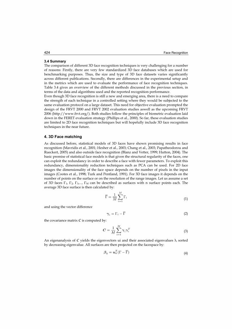
Face Recognition 424
3.4 Summary
The comparison of different 3D face recognition techniques is very challenging for a number of reasons: Firstly, there are very few standardized 3D face databases which are used for benchmarking purposes. Thus, the size and type of 3D face datasets varies significantly across different publications. Secondly, there are differences in the experimental setup and in the metrics which are used to evaluate the performance of face recognition techniques. Table 3.4 gives an overview of the different methods discussed in the previous section, in terms of the data and algorithms used and the reported recognition performance. Even though 3D face recognition is still a new and emerging area, there is a need to compare the strength of each technique in a controlled setting where they would be subjected to the same evaluation protocol on a large dataset. This need for objective evaluation prompted the design of the FRVT 2000 and FRVT 2002 evaluation studies aswell as the upcoming FRVT 2006 (http://www.frvt.org/). Both studies follow the principles of biometric evaluation laid down in the FERET evaluation strategy (Phillips et al., 2000). So far, these evaluation studies are limited to 2D face recognition techniques but will hopefully include 3D face recognition techniques in the near future.
4. 3D Face matching
As discussed before, statistical models of 3D faces have shown promising results in face recognition (Mavridis et al., 2001; Hesher et al., 2003; Chang et al., 2003; Papatheodorou and Rueckert, 2005) and also outside face recognition (Blanz and Vetter, 1999; Hutton, 2004). The basic premise of statistical face models is that given the structural regularity of the faces, one can exploit the redundancy in order to describe a face with fewer parameters. To exploit this redundancy, dimensionality reduction techniques such as PCA can be used. For 2D face images the dimensionality of the face space depends on the number of pixels in the input images (Cootes et al., 1998; Turk and Pentland, 1991). For 3D face images it depends on the number of points on the surface or on the resolution of the range images. Let us assume a set of 3D faces 1, 2, 3,..., M can be described as surfaces with n surface points each. The average 3D face surface is then calculated by:
(1)
and using the vector difference
(2)
the covariance matrix C is computed by:
(3)
An eigenanalysis of C yields the eigenvectors ui and their associated eigenvalues i sorted by decreasing eigenvalue. All surfaces are then projected on the facespace by:
(4)

3D Face Recognition 425
where k = 1, ...,m. In analogy to active shape models in 2D (Cootes et al., 1995), every 3D surface can then be described by a vector of weights T = [ 1, 2, ..., m], which dictates how much each of the principal eigenfaces contributes to describing the input surface. The value of m is application and data-specific, but in general a value is used such that 98% of the population variation can be described. More formally (Cootes et al., 1995):
(5)
The similarity between two faces A and B can be assessed by comparing the weights A and B which are required to parameterize the faces. We will use two measurements for
measuring the distance between the shape parameters of the two faces. The first one is the Euclidean distance which is defined as:
(6)
In addition it is also possible calculated the distance of a face fromthe feature-space (Turk and Pentland, 1991). This effectively calculates how “face”-like the face is. Based on this, there are four distinct possibilities: (1) the face is near the feature-space and near a face class (the face is known), (2) the face is near the feature-space but not near a face class (face is unknown), (3) the face is distant from the feature-space and face class (image not a face) and finally (4) the face distant is from feature-space and near a face class (image not a face). This way images that are not faces can be detected. Typically case (3) leads to false positives in most recognition systems. By computing the sample variance along each dimension one can use the Mahalanobis distance to calculate the similarity between faces (Yambor et al., 2000). In the Mahalanobis space, the variance along each dimension is normalized to one. In order to compare the shape parameters of two facial surfaces, the difference in shape parameters is divided by the corresponding standard deviation :
(7)
5. Construction of 3D statistical face models using registration
A fundamental problem when building statistical models is the fact that they require the determination of point correspondences between the different shapes. The manual identification of such correspondences is a time consuming and tedious task. This is particularly true in 3D where the amount of landmarks required to describe the shape accurately increases dramatically compared to 2D applications.
5.1 The correspondence problem
The key challenge of the correspondence problem is to find points on the facial surface that correspond, anatomically speaking, to the same surface points on other faces (Beymer and Poggio, 1996). It is interesting to note that early statistical approaches for describing faces

Face Recognition 426
did not address the correspondence problem explicitly (Turk and Pentland, 1991; Kirby and Sirovich, 1990).
Anatomical points landmarked Points Landmark Description
Glabella Area in the center of the forehead between the eyebrows, above the nose which is slightly protruding (1 landmark).
Eyes Both the inner and outer corners of the eyelids are landmarked (4 landmarks).
NasionThe intersection of the frontal and two nasal bones of the human skull where there is a clearly depressed area directly between the eyes above the bridge of the nose (1 landmark).
Nose tip The most protruding part of the nose (1 landmark). Subnasal The middle point at the base of the nose (1 landmark).
Lips Both left and right corners of the lips aswell as the top point of the upper lip and the lowest point of the lower lip (4 landmarks).
Gnathion The lowest and most protruding point on the chin (1 landmark).
Table 2. The 13 manually selected landmarks chosen because of their anatomical distinctiveness
The gold standard to establish correspondence is by using manually placed landmarks to mark anatomically distinct points on a surface. As this can be a painstaking and error-prone process, several authors have proposed to automate this by using a template with annotated landmarks. This template can be then registered to other shapes and the landmarks can be propagated to these other shapes (Frangi et al., 2002; Rueckert et al., 2003). Similarly, techniques such as optical flow can be used for registration. For example, correspondences between 3D facial surfaces can be estimated by using optical flow on 2D textures to match anatomical features to each other Blanz and Vetter (1999). Some work has been done on combining registration techniqueswith a semi-automatic statistical technique, such as active shape models, in order to take advantage of the strengths of each (Hutton, 2004). Yet another approach defines an objective function based on minimum description length (MDL) and thus treats the problem of correspondence estimation as an optimization problem (Davies, 2002). Another way of establishing correspondence between points on two surfaces is by analyzing their shape. For example, curvature information can be used to find similar areas on a surface in order to construct 3D shape models (Wang et al., 2000). Alternatively, the surfaces can be decimated in such a way that eliminates points from areas of low curvature. High curvature areas can then assumed to correspond to each other and are thus aligned (Brett and Taylor, 1998; Brett et al., 2000).
5.2 Landmark-based registration
One way of achieving correspondences is by using landmarks that are manually placed on 3D features of the face. The landmarks should be placed on anatomically distinct points of the face in order to ensure proper correspondence. However, parts of the face such as the cheeks are difficult to landmark because there are no uniquely distinguishable anatomical points across all faces. It is important to choose landmarks that contain both local feature information (eg. the size of the mouth and nose) as well as the overall size of the face (eg. the location of the eyebrows). Previous work on 3D face modelling for classification has shown
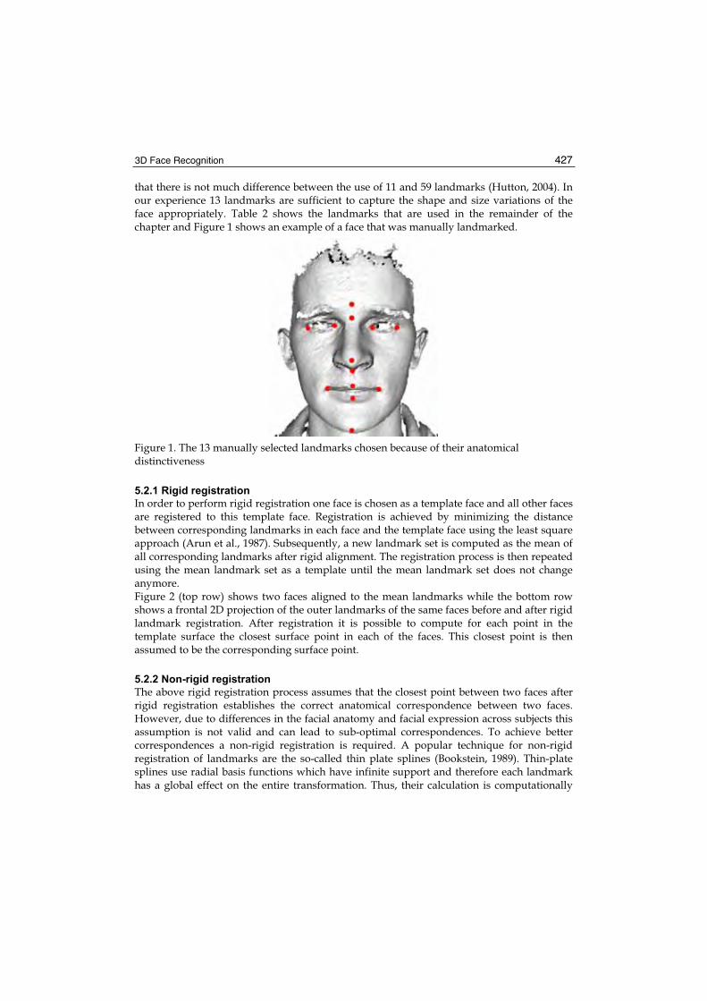
3D Face Recognition 427
that there is not much difference between the use of 11 and 59 landmarks (Hutton, 2004). In our experience 13 landmarks are sufficient to capture the shape and size variations of the face appropriately. Table 2 shows the landmarks that are used in the remainder of the chapter and Figure 1 shows an example of a face that was manually landmarked.
Figure 1. The 13 manually selected landmarks chosen because of their anatomical distinctiveness
5.2.1 Rigid registration
In order to perform rigid registration one face is chosen as a template face and all other faces are registered to this template face. Registration is achieved by minimizing the distance between corresponding landmarks in each face and the template face using the least square approach (Arun et al., 1987). Subsequently, a new landmark set is computed as the mean of all corresponding landmarks after rigid alignment. The registration process is then repeated using the mean landmark set as a template until the mean landmark set does not change anymore. Figure 2 (top row) shows two faces aligned to the mean landmarks while the bottom row shows a frontal 2D projection of the outer landmarks of the same faces before and after rigid landmark registration. After registration it is possible to compute for each point in the template surface the closest surface point in each of the faces. This closest point is then assumed to be the corresponding surface point.
5.2.2 Non-rigid registration
The above rigid registration process assumes that the closest point between two faces after rigid registration establishes the correct anatomical correspondence between two faces. However, due to differences in the facial anatomy and facial expression across subjects this assumption is not valid and can lead to sub-optimal correspondences. To achieve better correspondences a non-rigid registration is required. A popular technique for non-rigid registration of landmarks are the so-called thin plate splines (Bookstein, 1989). Thin-plate splines use radial basis functions which have infinite support and therefore each landmark has a global effect on the entire transformation. Thus, their calculation is computationally

Face Recognition 428
inefficient. Nevertheless, thin-plate splines have been widely used in medical imaging as well as for the alignment of 3D faces using landmarks (Hutton, 2004).
Figure 2. Rigid registration of faces using landmarks. The top rowshows the two faces aligned to the mean landmarks. The bottom row shows a frontal 2D projection of the outer landmarks of the same faces before and after registration
An alternative approach for the non-rigid registration of 3D faces is to use a so-called free-form deformation (FFD) (Sederberg and Parry, 1986) which can efficiently model local deformations. B-spline transformations, contrary to thin-plate splines, have local support, which means that each control point influences a limited region. Furthermore, the computational complexity of calculating a B-spline is significantly lower than a thin-plate spline. In the following, a nonrigid registration algorithm for landmarks based on multi-resolution B-splines is proposed. Lee et al. described a fast algorithm for interpolating and approximating scattered data using a coarse-to-fine hierarchy of control lattices in order to generate a sequence of bicubic B-spline function whose sum approximates the desired interpolation function (Lee et al., 1997). We adopt this approach in order to calculate an optimal free-form deformation for two given sets of 3D landmarks. A rectangular grid of control points is initially defined (Figure 3) as a bounding box of all landmarks. The control points of the FFD are deformed in order to precisely align the facial landmarks. Between the facial landmarks the FFD provides a smooth interpolation of the deformation at the landmarks. The transformation is defined by a nx × ny × nz grid of control point vectors lmn with uniform spacing :
(8)

3D Face Recognition 429
where and and where Bi, Bj , Bk represent the B-spline basis functions which define the contribution of each control point based on its distance from the landmark (Lee et al., 1996, 1997):
Figure 3. A free-formdeformation and the corresponding mesh of control points
Given a moving point set (source) and a fixed point set , the algorithm estimates a set of displacement vectors d = p – q
associated with the latter. The output is an array of displacement vectors lmn for the control points which provides a least squares approximation of the displacement vectors. Since B-splines have local support, each source point pe is affected by the closest 64 control points. The displacement vectors of the control points associated with this source point can be denoted as ijk:
(9)
where wijk = Bi(r) Bj(s) Bk(t) and i, j, k = 0, 1, 2, 3. Because of the locality of B-splines, the spacing of control points has a significant impact on the quality of the least squares approximation and the smoothness of the deformation: Large control point spacings lead to poor approximations and high smoothness whereas small control point spacings lead to good approximations but less smoothness. To avoid these problems, a multilevel version of the B-spline approximation is used (Lee et al., 1997). In this approach an initial coarse grid is used initially and then iteratively subdivided to enable closer and closer approximation between

Face Recognition 430
two point sets. Before every subdivision of the grid the current transformation T is applied to points p and the displacement vectors d are recomputed.
5.3 Surface-based registration
A drawback of the registration techniques discussed in the previous section is the need for landmarks. The identification of landmarks is a tedious and time-consuming step which typically requires a human observer. This introduces inter- and intra-observer variability into the landmark identification process. In this section we will focus on surface-based registration techniques which do not require landmarks.
5.3.1 Rigid registration
The most popular approach for surface registration is based on the iterative closest point (ICP)algorithm (Besl and McKay, 1992): Given two facial surfaces, i.e. a moving face A = {ai} and a fixed (template) face B = {bi}, the goal is to estimate the optimal rotation R and translation tthat best aligns the faces. The function to be minimized is the mean square difference function between the corresponding points on the two faces:
(10)
where pointswith the same index correspond to each other. The correspondence is established by looping over each point a on face A and finding the closest point, in Euclidean space, on face B:
(11)
This process is repeated until the optimal transformation is found. As before it is possible after this registration to compute for each point in the template surface the closest surface point in each of the faces. This closest point is then assumed to be the corresponding surface point.
5.3.2 Non-rigid registration
As before, rigid surface registration can only correct for difference in pose but not for differences across the facial anatomy and expression of different subjects. Thus, the correspondences obtained fromrigid surface registration are sub-optimal. This is especially pronounced in areas of high curvature where the faces might differ significantly, such as around the lips or nose. As a result the correspondence established between surface points tends to be incorrect. In this section we propose a technique for non-rigid surface registration which aims to improve correspondences between surfaces. Given surfaces A and B, made up of two point sets a and b, the similarity function that we want to minimize is:
(12)
where T nonrigid is a non-rigid transformation. A convienient model for such a non-rigid transformation is the FFD model described in eq. (8). Once more one can assume that the

3D Face Recognition 431
correspondence between surface points is unknown. In order to pair points on two surfaces to each other, just as with ICP, one can assume that corresponding points will be closer to each other than non-corresponding ones. A distance metric d is defined between an individual source point a and a target shape B:
(13)
Using this distance metric the closest point in B from all points in A is located. Let Y denote the resulting set of closest points and C the closest point operator:
(14)
After closest-point correspondence is established, the point-based non-rigid registration algorithm can be used to calculate the optimal non-rigid transformation Tnonrigid. This is represented here by the operator . In order for the deformation of the surfaces to be smooth, a multi-resolution approach was adopted, where the control point grid of the transformation is subdivided iteratively to provide increasing levels of accuracy. The non-rigid surface registration algorithm is displayed in Listing 1.
Listing 1 The non-rigid surface registration algorithm. 1: Start with surfaces A and a target point set B.2: Set subdivision counter k = 0, A(0) = A and reset Tnonrigid.3: repeat4: Find the closest points between A and B by: Y (k) = C (A(k), B)5: Compute the ideal non-rigid transformation to align Y (k) and A(0) by:
(see section 5.2.2).
6: Apply the transformation: 7: until k equals user-defined maximum subdivisions limit
Figure 4 shows a colour map of the distance between two faces after rigid and non-rigid surface registration. It can be clearly seen that the non-rigid surface registration improves the alignment of the faces when compared to rigid surface registration. Similarly, non-rigid surface registration also better aligns the facial surfaces than non-rigid landmark registration:Figure 5 (a) shows a color map of the distance between two paces after landmark-based registration. Notice that the areas near the landmarks (eyes, mouth, nose, chin) are much better aligned than other areas. Figure 5 (b) shows a colour map after surface-based registration. In this case the registration has reduced the distances between faces in all areas and provides a better alignment.
6. Evaluation of 3D statistical face models
To investigate the impact of different registration techniques for correspondence estimation on the quality of the 3D model for face recognition, we have constructed a 3D statistical face model using 150 datasets (University of Notre Dame, 2004). These datasets were acquired using a Minolta VIVID 910 camera which uses a structured light sensor to scan surfaces. A typical face consists of about 20,000 points. Figure 6 shows an example face.

Face Recognition 432
(a) (b) Figure 4. Two faces after (a) rigid and (b) non-rigid surface registration. The colour scale indicates the distance between the closest surface points
(a) (b) Figure 5. Two faces after (a) rigid landmark registration and (b) rigid landmark registration followed by non-rigid surface registration. The colour scale indicates the distance between the closest surface points
Figure 6. Example of a Notre Dame dataset
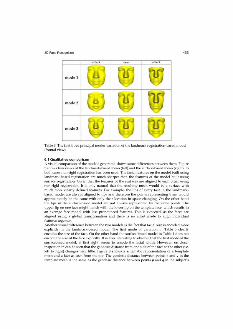
3D Face Recognition 433
Table 3. The first three principal modes variation of the landmark registration-based model (frontal view)
6.1 Qualitative comparison
A visual comparison of the models generated shows some differences between them. Figure 7 shows two views of the landmark-based mean (left) and the surface-based mean (right). In both cases non-rigid registration has been used. The facial features on the model built using landmark-based registration are much sharper than the features of the model built using surface registration. Given that the features of the surfaces are aligned to each other using non-rigid registration, it is only natural that the resulting mean would be a surface with much more clearly defined features. For example, the lips of every face in the landmark-based model are always aligned to lips and therefore the points representing them would approximately be the same with only their location in space changing. On the other hand the lips in the surface-based model are not always represented by the same points. The upper lip on one face might match with the lower lip on the template face, which results in an average face model with less pronounced features. This is expected, as the faces are aligned using a global transformation and there is no effort made to align individual features together. Another visual difference between the two models is the fact that facial size is encoded more explicitly in the landmark-based model. The first mode of variation in Table 3 clearly encodes the size of the face. On the other hand the surface-based model in Table 4 does not encode the size of the face explicitly. It is also interesting to observe that the first mode of the surfacebased model, at first sight, seems to encode the facial width. However, on closer inspection in can be seen that the geodesic distance from one side of the face to the other (i.e. left to right) changes very little. Figure 8 shows a schematic representation of a template mesh and a face as seen from the top. The geodesic distance between points x and y in the template mesh is the same as the geodesic distance between points p and q in the subject’s

Face Recognition 434
face. In other words the “height” and the “width” of the template face that is used to resample a facial surface does not change significantly. What does change and is therefore encoded in the first principal component of the ICP-based model is the “depth” (protrusion) of the template face.
Table 4. The first three principal modes variation of the surface-based registration model (frontal view)
Figure 7. Comparison of the mean face from the landmark-based model mean (left) and a surface-based model mean (right)

3D Face Recognition 435
Figure 8. Once the faces are registered using surface the closest points are selected. The geodesic distance between points x and y in the template mesh and p and q in the subject’s face remains relatively unchanged
6.2 Quantitative comparison
The differences of the visual aspects of the 3D statistical face models do not necessarily describe the quality of the face models. To assess the model quality more quantitatively, several generic objective measures such as generalisability, specificity and compactness can be used.
6.2.1 Generalization ability
The generalization ability of a face model is its ability to represent a face that is not part of the training set. This is of importance, as the model needs to be able to generalize to unseen examples. Otherwise the model is overfitting to the training set. Generalization ability can be measured using leave-one-out reconstruction (Davies, 2002; Hutton, 2004). First, a face model built using datasets { } and leaving one face i out. Then, the left-out face is projected into the facespace defined by u. This facespace is created using the remaining 149 faces:
(15)
The face i is then reconstructed using its face parameters s generating a surface i (s):
(16)
where s is the number of shape parameters . The average square approximation error between the original face i and the reconstructed i can be measured as:
(17)
This process is repeated for all faces. For a more robust assessment of the model, the generalization ability was measured as a function of the number s of shape parameters .The mean square approximation error is the generalization ability score

Face Recognition 436
(18)
where M is the total number of faces used. For two models X and Y, if GX (s) GY (s) for all sand GX(s)<GY(s) for some s, then the generalization ability of model X is better than that of model Y . In this case s is the number of shape parameters that are used to build the left-out face. In order to assess the differences between the models’ generalization scores, the standard error of each model has to be calculated (Spiegel and Stephens, 1998):
(19)
where M is the total number of faces used to build the model and is the sample standard deviation of G(s) defined as:
(20)
Figure 9. The Generalization ability of the landmark-based and surface-based models. Note that in the graph the better a model generalizes to unseen examples the lower its generalization scores are. The error bars are computed as shown in eq. 19 and they show a relatively small standard error in G(s) which allows us to safely conclude that the differences in the generalization scores of the two models are significant
As can be seen in Figure 9 the 3D statistical model built using surface registration has greater capacity to explain unseen examples than the model built using landmark

3D Face Recognition 437
registration. In particular, this is most obvious when only a few parameters (between 1 to 30) are used to encode each face.
6.2.2 Specificity
Specificity measures the ability of the face model to generate face instances that are similar to those in the training set. To test the specificity N randomfaces were generated as a function of s, the number of face parameters . The generated faces are then compared to the closest faces in the training set:
(21)
For two models X and Y , if SX(s) SY (s) for all s and SX(s) < SY (s) for some s then method Xbuilds a more specific model than method Y . Once again the standard error of each model has to be calculated in order to be able to assess whether the differences between the two models are significant:
(22)
To calculate the specificity 500 random faces were generated. Figure 10 shows that the model built using surface registration is also significantly more specific than the model built using landmark registration.
6.2.3 Compactness
Compactness measures the ability of the model to reconstruct an instance with as few parameters as possible. A compact model is also one that has as little variance as possible, and it is described as a plot of the cumulative covariance matrix:
(23)
To assess the significance of the differences, the standard error in C(s) is calculated once again. The standard deviation in the ith mode is given by (Spiegel and Stephens, 1998):
(24)
where i is the ith eigenvalue of the covariance matrix. The standard error is then given by:
(25)
Figure 11 shows that the model built using surface registration is significantly more compact than the model built using landmark registration.

Face Recognition 438
Figure 10. The specificity scores of the landmark-based and surface-based models. Small standard error in S(s) (as shown fromthe error bars) also allows for us to conclude safely that the difference in specificity scores is indeed significant
Figure 11. The compactness scores of the landmark-based and surface-based models. The standard error bars indicate the likely error of C(s) allowing one once more to conclude that there is significant difference between the compactness scores of the two models

3D Face Recognition 439
6.3 Application to face recognition
The differences in the statistical models describe some visual aspects of the 3D face and do not necessarily describe their ability to performface recognition. In order to assess the quality of the model-building methods for face recognition, we measured performance in three tasks: verification, open-set identification and closed-set identification as proposed in the FERET evaluation protocol (Phillips et al., 2000). Because of the small number of datasets (150 subjects × 2 samples per subject) we decided not to split the data into three groups as in the FERET protocol in order to perform open-set identification subjects. Instead we divided the subjects into two pools, the gallery set and the probe set . The first group comprises of faces that are known to the system and are referred to as the gallery . The other set is the probe set , containing different biometric samples of the same subjects contained in the gallery set. To perform open-set identification we need to calculate the False Acceptance (PFA) and Correct Detection and Identification (PDI) rate. The PFA is calculated by:
(26)
This means that for every face in we check if there is any face in other than the face belonging to the same subject that would cause a false alarm, given a threshold . The PDI is defined as:
(27)
The open set identification is plotted agains the PDI rate when PFA = 1 – PDI . The second measure reported is the rank 1 rate. The cumulative count in this case is given by:
(28)
The closed-set identification for rank 1, PI (1), is the fraction of probes at rank 1 and is described by:
(29)
For calculating the verification rate we use the round-robin method (Phillips et al., 2004), which is designed for two groups and :
(30)
where is set to a value so that PFA = 1%. In all experiments, all faces in the probe and gallery sets are projected into the facespace and their parameters are used for similarity comparisons as described in Section 4. Using the Euclidean metric to measure similarities between the faces, rank 1 identification as well as verification was performed to describe the task-specific effectiveness of the models. Figure 12 shows the rank 1 rates of the various models. The difference between them is clear as the surface-based models perform significantly better than the landmark-based models,

Face Recognition 440
achieving rank 1 rates of 100%. Figure 13 shows the verification rates of the various models. Again, the surface-based models outperform the landmark-based models. Finally, the open-set identification rates for the different models are shown in Figure 14.
Figure 12. Rank 1 (PI (1)) rates of the various 3D statistical face models
Figure 13. Verification rates of the various 3D statistical face models

3D Face Recognition 441
Figure 14. Open-set identification rates of the various 3D statistical face models
7. Disscussion and Conclusions
This chapter has provided an overview of 3D face recognition techniques. In particular we have shown that 3D statistical face models are well suited for 3D face recognition. A key challenge in the construction of these statistical models is the estimation of correspondences across the faces in the training set. The quality of these correspondences can be directly linked to the quality of the model for task-specific applications such as face recognition. Our results have shown that surface-based registration techniques produce much better models than landmark-based registration techniques in terms of their face recognition performance. The models built using surface-based registration are also more specific, compact and generalizes better to unseen examples. In principle it should also be possible to construct 3D face models which are optimal in some sense, e.g. with regard to a certain performance metric in face recognition. This would entail an optimization of the correspondences across all faces (e.g. by using a groupwise registration algorithm (Cootes et al., 2004)) in such a way that the resulting model produces the best possible face recognition performance. Finally, the 3D statistical face models discussed so far include only shape information. Of course texture is also a very important aspect of the face and should be included into the 3D statistical face model (similarily to the 3D morphable face model (Blanz and Vetter, 1999)).

Face Recognition 442
8. References
Ackermann, B. and Bunke, H., t. . C. (2000). In 15th International Conference on Pattern Recogni- tion, pages 809–813.
Ansari, A. and Abdel-Mottaleb, M. (2003a). 3D face modelling using two orthogonal views and a generic face model. In International Conference on Multimedia and Expo, pages 289–292.
Ansari, A. and Abdel-Mottaleb, M. (2003b). 3D face modelling using two views and a generic face model with application to 3D face recognition. In IEEE Conference on Advanced Video and Signal Based Surveillance, pages 37–44.
Arun, K., Huang, T., and S.D., B. (1987). Least squares fitting of two 3D point sets. IEEETransactions on Pattern Analysis and Machine Intelligence, 9(5):698–700.
Besl, P. and McKay, N. (1992). A method for registration of 3D shapes. IEEE Transactions on Pattern Analysis and Machine Intelligence, 14(2):239–256.
Beumier, C. and Acheroy, M. (2000). Automatic 3D face authentication. Image and Vision Computing, 18(4):315–321.
Beumier, C. and Acheroy, M. (2001). Face verification from 3D and grey level clues. Pattern Recognition Letters, 22:1321–1329.
Beymer, D. and Poggio, T. (1996). Image representations for visual learning. Science,272:1905–1909.
Blanz, V., Grother, P., Phillips, J., and Vetter, T. (2005). Face recognition based on frontal views generated fromnon-frontal images. In IEEE Conference on Computer Vision and Pattern Recognition (CVPR), pages 454–461.
Blanz, V., Romdhani, S., and Vetter, T. (2002). Face identification across different poses and illuminations with a 3D morphable model. In International Conference on Automatic Face and Gesture Recognition, pages 202–207.
Blanz, V. and Vetter, T. (1999). A morphable model for the synthesis of 3D faces. In SIGGRAPH, pages 187–194.
Bookstein, F. L. (1989). Principal warps: thin-plate splines and the decomposition of deformations. IEEE Transactions on Pattern Analysis and Machine Intelligence,11(6):567–585.
Brett, A., Hill, A., and Taylor, C. (2000). A method of automatic landmark generation for automated 3D PDM construction. Image and Vision Computing, 18:739–748.
Brett, A. and Taylor, C. (1998). A method of automatic landmark generation for automated 3D PDMconstruction. In 9th BritishMachine Vision Conference Proceedings, pages 914–923. Springer.
Bronstein, A., Bronstein,M., and Kimmel, R. (2003). Expression-invariant 3D face recognition. In International Conference on Audio- and Video-Based Person Authentication, pages 62– 70.
Bronstein, A., Bronstein, M., and Kimmel, R. (2005). Three-dimensional face recognition. In- ternational Journal of Computer Vision, 64:5–30.
Bruce, V. (1982). Visual and non-visual coding processes in face recognition. British Journal of Psychology, 73:105–116.
Bruce, V. (1988). Recognizing faces. Lawrence Erlbaum Associates. Bruce, V. (1994). Stability from variation: the case of face recognition. Quarterly Journal of
Experimental Psychology, 47(1):5–28.

3D Face Recognition 443
Bruce, V. and Langton, S. (1994). The use of pigmentation and shading information in recognising the sex and identities of faces. Perception, 23:803–822.
Cartoux, J., LaPreste, J., and Richetin, M. (1989). Face authentication or recognition by profile extraction from range images. In Workshop on Interpretation of 3D Scenes, pages 194– 199.
Chang, K., Bowyer, K., and Flynn, P. (2003). Face recognition using 2D and 3D facial data. In Multimodal User Authentication Workshop, pages 25–32.
Chua, C., Han, F., and Ho, Y. (2000). 3D human face recognition using point signature. In International Conference on Face and Gesture Recognition, pages 233–238.
Chua, C. and Jarvis, R. (1997). Point signatures - a new representation for 3D object recognition. International Journal of Computer Vision, 25(1):63–85.
Cootes, T., Edwards, G., and Taylor, C. (1998). Active appearance models. In EuropeanConference of Computer Vision (ECCV), pages 484–498.
Cootes, T., Marsland, S., Twining, C., Smith, K., and Taylor, C. (2004). Groupwise diffeomorphic non-rigid registration for automatic model building. In European Conference on Computer Vision (ECCV), pages 316–27.
Cootes, T., Taylor, C., Cooper, D., and Graham, J. (1995). Active shape models - their training and application. Computer Vision and Image Understanding, 61:18–23.
Davies, R. (2002). Learning Shape: Optimal Models for Analysing Natural Variability. PhD thesis, University of Manchester.
Frangi, A., Rueckert, D., Schnabel, J., and Niessen, W. (2002). Automatic construction of multiple-object three-dimensional statistical shape models: Application to cardiac modeling. IEEE Transactions on Medical Imaging, 21(9):1151–1166.
G¨okberk, B., Salah, A., and Akarun, L. (2005). Rank-based decision fusion for 3D shape-based face recognition. In International Conference on Audio- and Video-based Biometric Person Authentication, pages 1019–1028.
Gordon, G. (1992). Face recognition based on depth and curvature features. In IEEEComputer Vision and Pattern Recognition (CVPR), pages 808–810.
Gross, R., Matthews, I., and Baker, S. (2002). Eigen light-fields and face recognition across pose. In International Conference on Automatic Face and Gesture Recognition.
Heisele, B., Serre, T., Pontil, M., and Poggio, T. (2001). Component-based face detection. In IEEE Conference on Computer Vision and Pattern Recognition (CVPR), pages 657–662.
Hesher, C., Srivastava, A., and Erlebacher, G. (2003). A novel technique for face recognition using range imaging. In International Symposium on Signal Processing and Its Applications, pages 201–204.
Hietmeyer, R. (2000). Biometric identification promises fast and secure processing of airline passengers. The International Civil Aviation Organization Journal, 55(9):10–11.
Hill, H. and Bruce, V. (1996). Effects of lighting on matching facial surfaces. Journal of Experimental Psychology: Human Perception and Performance, 22:986–1004.
Hill, H., Schyns, P., and Akamatsu, S. (1997). Information and viewpoint dependence in face recognition. Cognition, 62:201–202.
Huang, J., Heisele, B., and Blanz, V. (2003). Component-based face recognition with 3D morphable models. In International Conference on Audio- and Video-Based Person Authentication.
Hutton, T. (2004). Dense Surface Models of the Human Face. PhD thesis, University College London.

Face Recognition 444
Johnston, A., Hill, H., and Carman, N. (1992). Recognizing faces: effects of lighting direction, inversion and brightness reversal. Perception, 21:365–375.
Kakadiaris, I., Passalis, G., Theoharis, T., Toderici, G., Konstantinidis, I., and Murtuza, N. (2005). Multimodal face recognition: combination of geometry with physiological information. Number 2, pages 1022 – 1029.
Kim, T. and Kittler, J. (2005). Locally linear discriminant analysis for multimodally distributed classes for face recognition. IEEE Transactions on Pattern Analysis and Machine Intelligence, 27(3):318–327.
Kirby, M. and Sirovich, L. (1990). Application of the Karhunen-Lo´eve procedure for the characterization of human faces. IEEE Transactions on Pattern Analysis and Machine Intelligence, 12(1):103–108.
Lanitis, A., Taylor, C., and Cootes, T. (1995). Automatic face identification systemusing flexible appearance models. Image and Vision Computing, 13(5):393–401.
Lee, J. andMilios, E. (1990). Matching range images of human faces. In InternationalConference on Computer Vision (ICCV), pages 722–726.
Lee, S., Wolberd, G., Chwa, K., and Shin, S. (1996). Image metamorphosis with scattered feature constraints. IEEE Transactions on Visualization and Computer Graphics,2(4):337– 354.
Lee, S.,Wolberd, G., and Shin, S. (1997). Scattered data interpolationwith multilevel B-splines. IEEE Transactions on Visualization and Computer Graphics, 3(3):228–244.
Lee, Y. and Shim, J. (2004). Curvature-based human face recognition using depth-weighted hausdorff distance. In International Conference on Image Processing, pages 1429–1432.
Lee, Y., Song, H., Yang, U., Shin, H., and Sohn, K. (2005). Local feature based 3D face recognition. In International Conference on Audio- and Video-based Biometric Person Authentication, pages 909–918.
Li, Y., Gong, S., and Lidell,H. (2000). Support vector regression and classification based multiview face detection and recognition. In International Conference on Face and Gesture Recognition, pages 300–305.
Liu, C., Collin, C., Burton, A., and Chaurdhuri,A. (1999). Lighting direction affects recognition of untextured faces in photographic positive and negative. VisionResearch, 39:4003– 4009.
Lu, X., Colbry,D., and Jain, A. (2004). Matching 2.5D scans for face recognition. In International Conference on Pattern Recognition, pages 362–366.
Lu, X. and Jain, A. (2005a). Deformation analysis for 3D face matching. In IEEE Workshop on Applications of Computer Vision, pages 362–366.
Lu, X. and Jain, A. (2005b). Intergrating range and texture information for 3D face recognition. In 7th IEEE Workshop on Applications of Computer Vision, pages 155–163.
Maurer, T., Guigonis, D., Maslov, I., Pesenti, B., Tsaregorodtsev, A., West, D., and Medioni, G. (2005). Performance of geometrix activeidtm 3D face recognition engine on the frgc data. In IEEE Workshop on Face Recognition Grand Challenge Experiments.
Mavridis, N., Tsalakanidou, F., Pantazis, D., Malasiotis, S., and Strintzis, M. (2001). The hiscore face recognition application: Affordable desktop face recognition based on a novel 3D camera. In International Conference on Augmented Virtual Environments and 3D Images, pages 157–160.
Medioni, G. and Waupotitsch, R. (2003). Face recognition and modeling in 3D. In IEEEInternational Workshop on Analysis and Modeling of Faces and Gestures, pages 232–233.

3D Face Recognition 445
Moreno, A., Sanchez, A., Velez, J., and Diaz, F. (2003). Face recognition using 3D surfaceextracted descriptors. In Irish Machine Vision and Image Processing Conference.
Nagamine, T., Uemura, T., and Masuda, I. (1992). 3D facial image analysis for human identi- fication. In International Conference on Pattern Recognition, pages 324–327.
Pan, G.,Han, S.,Wu, Z., andWang, Y. (2005). 3D face recognition using mapped depth images. pages 175–175.
Pan, G., Wu, Z., and Pan, Y. (2003). Automatic 3D face verification from range data. pages 193–196.
Papatheodorou, T. and Rueckert, D. (2004). Evaluation of automatic 3D face recognition using surface and texture registration. In International Conference on Automated Face and Gesture Recognition, pages 321–326.
Papatheodorou, T. and Rueckert, D. (2005). Evaluation of 3 D face recognition using reg- istration and PCA. In Audio- and Video-based Biometric Person Authentication, pages 997–1009.
Passalis, G., Kakadiaris, I., Theoharis, T., Toderici, G., and Murtuza, N. (2005). Evaluation of 3D face recognition in the presence of facial expressions: an annotated deformable model approach. pages 1022 – 1029.
Phillips, J., Grother, P., and Michaels, R. (2004). Handbook of Face Recognition. Springer-Verlag.
Phillips, J., Moon, H., Rizvi, S., and Rauss, P. (2000). The FERET evaluation methodology for face-recognition algorithms. IEEE Transactions on Pattern Analysis and Machine Intelligence, 22(10):1090–1104.
Poggio, T. and Edelman, S. (1991). A network that learns to recognize 3D objects. Nature,343:263–266.
Prince, S. and Elder, J. (2006). Tied factor analysis for face recognition across large pose changes. In British Machine Vision Conference.
Rueckert, D., Frangi, A. F., and Schnabel, J. A. (2003). Automatic construction of 3-D statistical deformation models of the brain using nonrigid registration. IEEE Transactions on Medical Imaging, 22(8):1014–1025.
Russ, T., Koch, M., and Little, C. (2005). A 2D range hausdorff approach for 3D face recognition. In Computer Vision and Pattern Recognition, pages 1429–1432.
Schwartz, E., Shaw, A., and Wolfson, E. (1989). A numerical solution to the generalized mapmaker’s problem: flattening nonconvex polyhedral surfaces. IEEE Transactions on Pattern Analysis and Machine Intelligence, 11(9):1005–1008.
Sederberg, T. and Parry, S. (1986). Free-form deformation of solid geometric models. In Proceedings of the 13th Annual Conference on Computer Graphics and Interactive Techniques, pages 151–160.
Spiegel, M. and Stephens, L. (1998). Schaum’s Outline of Statistics. Schaum. Srivastava, A., Liu, X., and Hesher, C. (2003). Face recognition using optimal linear
components of face images. Journal of Image and Vision Computing, 24(3):291–299. Tanaka, H., Ikeda, M., and Chiaki, H. (1998). Curvature-based face surface recognition using
spherical correlation principal directions for curved object recognition. In International Conference on Automated Face and Gesture Recognition, pages 372–377.
Tarr, M. and Bulthoff, H. (1995). Is human object recognition better described by geon structural descriptions or by multiple views. Journal of Experimental Psychology,21:71–86.

Face Recognition 446
Tsalakanidou, F., Malassiotis, S., and Strintzis, M. (2004). Integration of 2D and 3D images for enhanced face authentication. In International Conference on Automated Face and Gesture Recognition, pages 266–271.
Tsalakanidou, F., Tzocaras, D., and Strintzis, M. (2003). Use of depth and colour eigenfaces for face recognition. Pattern Recognition Letters, 24:1427–1435.
Turk,M. and Pentland, A. (1991). Eigenfaces for recognition. Journal for Cognitive Neuroscience, 3(1):71–86.
University of Notre Dame (2002-2004). University of notre dame biometrics database distribution. http://www.nd.edu/ cvrl/UNDBiometricsDatabase.html.
Wang, Y., Chua, C., and Ho, Y. (2002). Facial feature detection and face recognition from 2D and 3D images. Pattern Recognition Letters, 23:1191–1202.
Wang, Y., Peterson, B., and Staib, L. (2000). Shape-based 3D surface correspondence using geodesics and local geometry. In IEEE Conference on Computer Vision and Pattern Recog- nition (CVPR), pages 644–651.
Wong, H., Chueng, K., and Ip, H. (2004). 3D head model classification by evolutionary optimization of the extended gaussian image representation. Pattern Recognition,37(12):2307–2322.
Wu, Y., Pan, G., and Wu, Z. (2003). Face authentication based on multiple profiles extracted fromrange data. In Audio- and Video-Based Biometric Person Authentication, pages 515– 522.
Xu, C.,Wang, Y., Tan, T., and Quan, L. (2004). Automatic 3D face recognition combining global geometric features with local shape variation information. In International Conference on Automated Face and Gesture Recognition, pages 308–313.
Yambor, W., Draper, B., and Beveridge, J. (2000). Empirical Evaluation Techniques in Computer Vision. Wiley.
Yin, L. and Yourst, M. (2003). 3D face recognition based on high-resolution 3D face modeling from frontal and profile views. In ACM Workshop on Biometric Methods and Applications, pages 1–8.

22
Multi-Modal Human Verification Using Face and Speech
Changhan Park1 and Joonki Paik2
1Advanced Technology R&D Center, Samsung Thales Co., Ltd., 2Graduate School of Advanced Imaging Science, Multimedia, and Film Chung-Ang University, Seoul
Korea
1. Introduction
Human biometric characteristics are unique, so it can hardly be duplicated (Kong et al. 2005). Such information includes; facial, speech, hands, body, fingerprints, and gesture to name a few. Face detection and recognition techniques are proven to be more popular than other biometric features based on efficiency and convenience (Kriegman et al. 2002; Liu et al. 2002). It can also use a low-cost personal computer (PC) camera instead of expensive equipments, and require minimal user interface. Face authentication has become a potential a research field related to face recognition. Face recognition differs from face authentication because the former has to determine the identity of an object, while the latter needs to verify the claimed identity of a user. Speech (Gu and Thomas 1999) is one of the basic communications, which is better than other methods in the sense of efficiency and convenience. Each a single biometric information, however, has its own limitation. For this reason, we present a multimodal biometric verification method to reduce false acceptance rate (FAR) and false rejection rate (FRR) in real-time. There have been many approaches for extracting meaningful features. Those include principal component analysis (PCA) (Rowley et al. 1998), neural networks (NN) (Rowley et al. 1998), support vector machines (SVM) (Osuna et al. 1997), hidden markov models (HMM) (Samaria and Young 1994), and linear discriminant analysis (LDA) (Belhumeur et al. 1997). In this chapter, we use the PCA algorithm with unsupervised learning to extract the face feature. We also use the HMM algorithm for extracting speech feature with supervised learning. This chapter is organized as follows: Section 2 and 3 describe feature extraction of face and speech using the PCA and HMM algorithms, respectively. Section 4 presents the design and structure of the proposed system. Section 5 presents experimental, and Section 6 concludes the paper with future research topics.
2. Face Extraction and Recognition
In this section, the proposed face extraction and recognition method will be presented. The proposed method can deal with both gray and color images. Depending on the type of images, an additional preprocessing step may be included so that facial features can be detected more easily.

Face Recognition 448
2.1 Face feature extraction and recognition
The proposed face feature extraction and recognition method is shown in Figure 1. The proposed method makes a new edge image using a 13×9 template in the face image. It can also estimate the face poses and normalize the size of detected face to 60×60. The normalized image is stored in multimodal database, and it trains the PCA module. The face recognition module distinguishes an input image from trained images.
Figure 1. Face feature extraction and recognition process
2.2 Face detection and building database using multi-layered relative edge map
In order to detect a face region and estimate face elements, we use the multi-layered relative edge map which can provide better result than just color-based methods (Kim et al. 2004). Such directional blob template can be determined according to the face size. More specifically, the template is defined so that the horizontal axis is longer than the vertical axis as shown in Figure 2(a). The central pixel of a template in a HW × image is defined as
( )xcc yxP ,= , which is created by averaging a 3×3 region. By using a ffff hw × directional
template for face components, the average intensity DirI of 8-neighborhood pixels is calculated on the central pixel, cP . As a result, cI , the brightness value at cP , and the brightness difference value can be obtained. The principal direction,
prd , and its magnitude,
|| prd , are also determined along the direction including the biggest brightness difference as
shown in Figure 2(b). N NENW
S SESW
EW
ffw
ffh
(a) (b) Figure 2. (a) Directional template (b) New direction for edge map

Multi-Modal Human Verification Using Face and Speech 449
Figure 3 shows the result of face separation by using the multi-layered relative edge map (MLREM) and with this result we make the face database.
(a) (b) (c)
Figure 3. (a) An input image, (b) the correspondingly created MLREM, and (c) the normalized database (60×60)
2.3 Unsupervised PCA and singular value decomposition (SVD)
In the process of PCA for pose estimation we compute covariance matrix C and its eigenvectors from training sets. Let Nxxx ,,, 21
be N training face vectors. By definition, C can then be estimated as (Zhang et al. 1997),
[ ]=
==N
k
Tkk
T XXN
XXEC1
1 . (1)
The training data set are packed into the following matrix
[ ]NxxxX ,,, 21= . (2)
The estimate of C can be approximately written as
TXXN
C 1= . (3)
To estimate the eigenvectors of C , we only need to find the eigenvectors of TXX . Even for images of moderate size, however, this is computational by complex. From the fundamental linear algebra (Sirivich and Kirby 1987), the eigenvectors of TXX can be found from eigenvectors of XX T , which are much easier to obtain. Suppose the rank of X is r , Nr ≤ .X has a SVD such as
=
=r
k
Tkkk vuX
1
λ , (4)
where kλ , ku , and kv respectively represent, singular values, left, and right singular vectors of X . ku and kv have the following relationship.
kk
k Xvuλ1= . (5)
Hence, we can easily find eigenface ku after finding kv . Recognized face classified using
( )=
−=m
iii trd
1
2 , where ir and it represent input pattern, pattern of train face, respectively.

Face Recognition 450
3. Speech Analysis and Feature Extraction
Speech recognition is classified into two categories in the sense of feature extraction method. One is to extract a linguistic information in speech signal, and the other is to extract an eigen specific of a speaker from speech signal (Rabiner and Juang 1998). The former performs extraction using the Mel-frequency cepstral coefficient (MFCC) based on the sense of hearing for human, and the latter extracts it with using the linear predictive coefficient (LPC) based on the sense of human speech. We adopt the latter because an individual has its own sense of speech. The LPC processing for speech recognition is shown as Figure 4. A simulation result of LPC in the proposed method is shown as Figure 5.
Figure 4. LPC processing for speech recognition
Figure 5. A simulation of LPC coefficient of 12th for Korean (open door)
3.1 HMM for speech recognition and verification
Speech verification calculates the cumulative distances with reference pattern when the test pattern is input. The reference patterns should be made in advance, and it can represent each speaker. This is classified in the pattern matching method that recognizes the pattern with calculated minimal cumulative distances and HMM. The HMM measures similarity

Multi-Modal Human Verification Using Face and Speech 451
with input pattern after modeling the speech signal statistically by extracting the feature from various speech waveforms. Training and verification for speech are shown in Figure 6. And the proposed method can solve following three problems:
(i) Evaluation problem: Given can observation sequence { }ToooO ,,, 21= and the model ),,( πλ BA= , (where, A represents transition probability, Boutput probability, and π initial probability), how to calculate ( )λ|OP - (it can be solved by using forward and backward algorithm.)
(ii) Learning problem: How to estimate the model parameter given { }ToooO ,,, 21= - (It can be solved by using Baum-Welch re-estimation.)
(iii) Decoding (recognition) problem: Given a model, how to get the best state sequence { }tqqqq ,,, 21= of { }ToooO ,,, 21= , where q represents the state sequence of model, t time. - (It can be solved by using the Viterbi algorithm.), where O represents specific vector for each frame.
Figure 6. Feature extraction and verification for speech

Face Recognition 452
4. Proposed Multimodal Biometric System
The proposed multimodal biometric recognition technique, can solve the fundamental limitations inherit to single biometric verification. The proposed verification system consists of the input, the learning, and the verification module. The input image of size 320×240 comes into the system in real-time together with the speech. In the learning module, the face image is trained under the PCA framework, and the speech is trained with HMM. Feature extraction is also accomplished in the learning module. The verification module validates the recognized data from the image and speech by using fuzzy logic. Personal information made is saved in the form of a code book, and used for verification and rejection.
4.1 Personal verification using multimodal biometric
In this subsection, we present a personal verification method as shown in Figure 6. The proposed method first detects the face area in an input image. The face verification module compares the detected face with the pre-stored code book of personal information. The speech verification module extracts and recognizes the end-point of speech, and authenticates it after comparing with the code book. Decision processes of face and speech use the proposed fuzzy logic algorithm. If the face and speech verification results coincide, there in no further processing. Otherwise the fuzzy logic is used to solve the mismatch problem. Therefore, if the face and speech is same to the personal information of the code book verification is accepted. Otherwise, it is rejected. The entire verification process is shown in Figure 7.
Figure 7. The entire verification process
4.2 Code book of personal face and speech information
In this subsection, the proposed personal information code book is described as shown in Figure 8. The face feature extraction block is trained by using the PCA algorithm with ten

Multi-Modal Human Verification Using Face and Speech 453
different images per single person. Each an individual probability information projects the data to the original image. Figure 9 shows a set of registered face images. The speech feature extraction block is trained by using the HMM algorithm with ten iterations per single person.
Figure 8. Created personal code book
Figure 9. Some images of registered person
4.3 Proposed fuzzy logic for improved verification
In this subsection, we present a decision method for the face and speech to be certificated using fuzzy logic. The proposed method extracts the candidate lists of recognized face images and speech as shown in Figure 10. In the face, F1 compares three images of the same person with an extracted face candidate. F2 and F3 respectively represent the cases with two and one images. For speech verification, S1 compares three speeches of the same person with an extracted candidate speaker. S2 and S3 respectively represent the cases with two and one speeches. Also, if the extracted candidate of face and speech is same, it is F0&S0 as shown in Figure 10. The verification of face and speech uses Mamdni's fuzzy inference (Manoj et al. 1998).
Figure 10. Fuzzy inference engine
The input fuzzy engine contains the recognized probability classified as shown in Figure 10, where ( )3,2,1,0&0,1,2,3 SSSSFFFFβ represents the coefficient of recognized probability. The basis rule is given as
0.0
5.0
0.1
)(
SPEECHisOThenCOMPLETEisRPIf
FACE
θ, (6)

Face Recognition 454
where { }3,2,1,0&0,1,2,3 SSSSFFFFR ∈ , and θO represents a pre-specificed threshold. The input membership function of fuzzy inference engine is shown in Figure 11. Finally, the predicted human verification result can be stored by using the Singleton’s fuzzifier, the product inference engine, and the average defuzzifier as
( ) ( ) ( )321max 131213 SFF OSOFOFP +++= . (7)
Figure 11. Input membership function of fuzzy engine
5. Experimental results
The proposed multimodal, biometric human recognition system is shown in Figure 12, which shows the result of face and speech extraction. Figure 13 shows the result of registered personal verification. Figure 14 shows the result of non registered person rejection.
(a) face detection and registration (b) speech detection and registration
Figure 12. The process to recognize face and speech
(a) person verification (b) person verification Figure 13. Accepted results
0.5
1.0 FACE COMPLETE SPEECH
0 0.5xPmax Pmax

Multi-Modal Human Verification Using Face and Speech 455
Figure 14. Rejected result for face and speech
The experimental result for the verification rate using the proposed method is summarized in Table 1. An experimental result of FAR given in Table 1 corresponds to 0.01%. In this case, the FAR can accept a person out of 100. Table 2 shows the result of the verification rate and FAR for the proposed method. As shown in Table 2, the proposed method can reduce FAR to 0.0001% and the impersonation to one person out of 10,000. Figure 15 shows that the proposed method can further reduce the equal error rate (EER).
verification rates(%) FAR(%) TestDB male female male female
face 98.5 0.01
speaker 97.37 0.01
Table 1. Verification rates of male and female
Test DB verification rate(%) FAR(%)
face & speaker 99.99 0.0001
Table 2. Verification rate of the proposed method
Figure 15. Error rate of the proposed method
6. Conclusions
In this chapter, we present a human verification method using combined face and speech information in order to improve the problem of single biometric verification. Single biometric verification has the fundamental problems of high FAR and FRR. So we present a

Face Recognition 456
multimodal, biometric human verification method to improve the verification rate and reliability in real-time. We use PCA for face recognition and HMM for speech recognition for real-time personal verification. As a result the proposed verification method can provides stable verification rate, and it overcomes the limitation of a single mode system. Based on the experimental results, we show that FRR can be reduced down to 0.0001% in the human multimodal interface method using both face and speech information.
7. References
Belhumeur, P.; Hespanha, J. and Kriegman, D. (1997) Eigenfaces vs fisherfaces: recognition using class specification linear projection. IEEE Transactions on Pattern Analysis and Machine Intelligence, Vol. 19, No. 7, (July 1997) Page(s) :711-720, 0162-8828.
Gu, Y. ; Thomas, T. (1999). A hybrid score measurement for HMM-based speaker verification. Proceedings of IEEE International Conference Acoustics, Speech, and Signal Processing, Vol. 1. pp. 317-320, March 1999.
Kim, Y. ; Park, C. and Paik, J. (2004). A new 3D active camera system for robust face recognition by correcting pose variation. Proceedings of International Conference Circuits and Systems, pp. 1482-1487, August 2004.
Kong, S.; Heo, J., Abidi, B., Paik, J., and Abidi, M. (2005). Recent advances in visual and infrared face recognition - A review. Computer Vision and Image Understanding, Vol. 97, No. 1, (January 2005) Page(s) :103-135, 1077-3142.
Kriegman, D.; Yang, M. and Ahuja, N. (2002). Detecting faces in images: a survey. IEEETransactions on Pattern Analysis and Machine Intelligence, Vol. 24, No. 1, (January 2002) Page(s) :34-58, 0162-8828.
Liu, X. ; Chen, T. and Kumar, V. (2002). On modeling variations for face authentication. Proceedings of International Conference Automatic Face and Gesture Recognition, pp. 369-374, May 2002.
Manoj, T.; Leena, J. and Soney, R. (1998). Knowledge representation using fuzzy petri nets-revisited. IEEE Transactions on Knowledge and Data Engineering, Vol. 10, No. 4, (August 1998) Page(s) :666-667, 1041-4347.
Osuna, E. ; Freund, R. and Girosi, F. (1997). Training support vector machines: an application to face detection. Proceeding of IEEE Conference Computer Vision and Pattern Recognition, pp. 130-136, 1997.
Rabiner, L.; Juang, B. (1998). Fundamentals of speech recognition, Prentice-Hall, 1993. Rowley, H. ; Baluja, S. and Kanade, T. (1998). Neural network-based face detection. IEEE
Transactions on Pattern Analysis and Machine Intelligence, Vol. 20, No. 1, (January 1998) Page(s) :203-208, 0162-8828.
Samaria, F. ; Young, S. (1994). HMM based architecture for face identification. Image and Vision Computing, Vol. 12, No. 8, (October 1994) Page(s) ;537-543, 0262-8856.
Sirivich, L. ; Kirby, M. (1987). Low-dimensional procedure for the characterization of human faces. Journal Optical Society of America A: Optics, Image Science, and Vision, Vol. 4, No. 3, (March 1987) Page(s):519-524.
Zhang, J. ; Yan, Y. and Lades, M. (1997). Face recognition: eigenface, elastic matching, and neural nets. Proceedings of IEEE, Vol. 85, No. 9, pp. 1423-1435, September 1997.

23
Face Recognition Using Optimized 3D Information from Stereo Images
Changhan Park1 and Joonki Paik2
1Advanced Technology R&D Center, Samsung Thales Co., Ltd., 2Graduate School of Advanced Imaging Science, Multimedia, and Film Chung-Ang University, Seoul
Korea
1. Introduction
Human biometric characteristics are unique, so it can not be easily duplicated [1]. Such information includes; facial, hands, torso, fingerprints, etc. Potential applications, economical efficiency, and user convenience make the face detection and recognition technique an important commodity compared to other biometric features [2], [3]. It can also use a low-cost personal computer (PC) camera instead of expensive equipments, and require minimal user interface. Recently, extensive research using 3D face data has been carried out in order to overcome the limits of 2D face detection and feature extraction [2], which includes PCA [3], neural networks (NN) [4], support vector machines (SVM) [5], hidden markov models (HMM) [6], and linear discriminant analysis (LDA) [7]. Among them, PCA and LDA methods with self-learning method are most widely used [3]. The frontal face image database provides fairly high recognition rate. However, if the view data of facial rotation, illumination and pose change is not acquired, the correct recognition rate remarkably drops because of the entire face modeling. Such performance degradation problem can be solved by using a new recognition method based on the optimized 3D information in the stereo face images. This chapter presents a new face detection and recognition method using optimized 3D information from stereo images. The proposed method can significantly improve the recognition rate and is robust against object’s size, distance, motion, and depth using the PCA algorithm. By using the optimized 3D information, we estimate the position of the eyes in the stereo face images. As a result, we can accurately detect the facial size, depth, and rotation in the stereo face images. For efficient detection of face area, we adopt YCbCr color format. The biggest object can be chosen as a face candidate among the candidate areas which are extracted by the morphological opening for the Cb and Cr components [8]. In order to detect the face characteristics such as eyes, nose, and mouth, a pre-processing is performed, which utilizes brightness information in the estimated face area. For fast processing, we train the partial face region segmented by estimating the position of eyes, instead of the entire face region. Figure 1. shows the block diagram of proposed algorithm. This chapter is organized as follows: Section 2 and 3 describe proposed stereo vision system and pos estimation for face recognition, respectively. Section 4 presents experimental, and section 5 concludes the chapter.
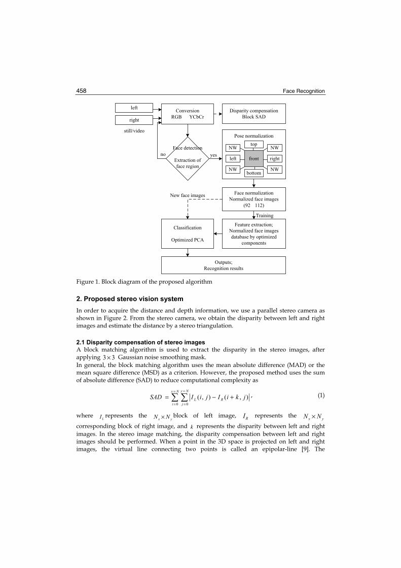
Face Recognition 458
left
right
still/video
Conversion
RGB YCbCr
Disparity compensation
Block SAD
Pose normalization
Face normalization
Normalized face images
(92 112)
NW NWtop
left rightfront
NW NWbottom
Feature extraction;
Normalized face images
database by optimized
components
Outputs;
Recognition results
Classification
Optimized PCA
Face detection
Extraction of
face region
yesno
New face images
Training
Figure 1. Block diagram of the proposed algorithm
2. Proposed stereo vision system
In order to acquire the distance and depth information, we use a parallel stereo camera as shown in Figure 2. From the stereo camera, we obtain the disparity between left and right images and estimate the distance by a stereo triangulation.
2.1 Disparity compensation of stereo images
A block matching algorithm is used to extract the disparity in the stereo images, after applying 33× Gaussian noise smoothing mask. In general, the block matching algorithm uses the mean absolute difference (MAD) or the mean square difference (MSD) as a criterion. However, the proposed method uses the sum of absolute difference (SAD) to reduce computational complexity as
=
=
=
=
+−=Nx
i
Ny
jRL jkiIjiISAD
0 0
),(),( , (1)
whereLI represents the
yx NN × block of left image, RI represents the yx NN ×
corresponding block of right image, and k represents the disparity between left and right images. In the stereo image matching, the disparity compensation between left and right images should be performed. When a point in the 3D space is projected on left and right images, the virtual line connecting two points is called an epipolar-line [9]. The

Face Recognition Using Optimized 3D Information from Stereo Images 459
corresponding blocks of the stereo images are matched on the epipolar-line with the same x-coordinate. The modified block matching algorithm based on 4×4 block is used for fast processing as shown in Figure 3.
Figure 2. Structure of a parallel stereo camera
Figure 3. Disparity compensation of stereo images
The proposed block matching algorithm can remove unnecessary operations and the performance of the proposed block matching algorithm is as good as the one of the global searching algorithm. The process of the proposed algorithm is as following. First, SAD is calculated at each row and then the minimum value of SAD at the corresponding row is obtained as
+−==
=
=
=k
Nx
k
Ny
jRL
RMIN jkiIjiIMINSAD
0 0
),(),( , (2)
Finally, the minimum SAD of entire image can be obtained as
= RMINMIN SADMINSAD . (3)

Face Recognition 460
Also, the disparity value between left and right images can be calculated as [2]
ktrightright −∗ = , ktleftleft +
∗ = . (4)
2.2 Scaling of the face images according to the distance
320×240 RGB color images including face region are used as an input image. For fast processing and reducing the effect for illumination changes, the RGB input image is converted to YCbCr image. By defining the color range for Asian’s face skin as
]127,77[=CbR and ]173,133[=CrR , a color-based image segmentation [10] is performed as
[ ] [ ]∈∩∈=
,0
),(),(,1),(
otherwiseRyxCrRyxCbif
yxS CrCb . (5)
By using the camera characteristics as given in Table 1, the distance can be measured as
][1080.86 3 mxx
bfDrl
××−
= , (6)
where b represents the width between cameras, f represents the focal length, and xl and xr
respectively represent the distances of left and right images. Also, the constant of 86.80×10³ represents the effective distance per pixel.
Item Characteristic Camera setting method binocular Camera setting width 65( )
Camera focus length(f) 3.6( )
Size 1 pixel 7.2×5.6( )Resolution width 512(dots)
Table 1. Camera’s component elements
For the 320x240 input images, the maximum distance of the disparity, rl xx − is equal to 320, and the minimum distance is equal to 1. The scaling according to the change of distance [11] is performed as
=1100
00
00
1
'
'
yx
ss
yx
y
x, (7)
where 'x , 'y represent the position after scaling processing, xs ,ys represent the scaling
factor, and x , y represent the current position. From the obtained distance in (6), the scaling factor of face image can be calculated as
( ) distdistdistx AVBV /×= , (8)
where distB , distV , and distA , and represent the basic distance, the established value by distance, and the obtained distance, respectively.
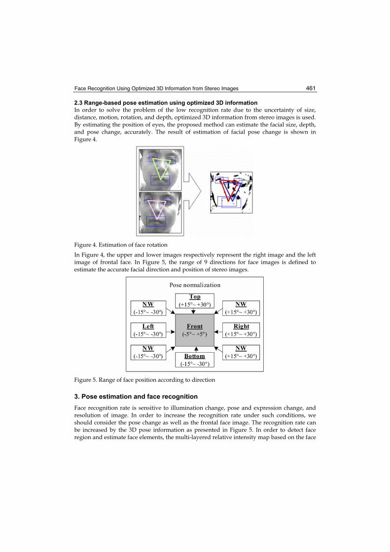
Face Recognition Using Optimized 3D Information from Stereo Images 461
2.3 Range-based pose estimation using optimized 3D information
In order to solve the problem of the low recognition rate due to the uncertainty of size, distance, motion, rotation, and depth, optimized 3D information from stereo images is used. By estimating the position of eyes, the proposed method can estimate the facial size, depth, and pose change, accurately. The result of estimation of facial pose change is shown in Figure 4.
Figure 4. Estimation of face rotation
In Figure 4, the upper and lower images respectively represent the right image and the left image of frontal face. In Figure 5, the range of 9 directions for face images is defined to estimate the accurate facial direction and position of stereo images.
Figure 5. Range of face position according to direction
3. Pose estimation and face recognition
Face recognition rate is sensitive to illumination change, pose and expression change, and resolution of image. In order to increase the recognition rate under such conditions, we should consider the pose change as well as the frontal face image. The recognition rate can be increased by the 3D pose information as presented in Figure 5. In order to detect face region and estimate face elements, the multi-layered relative intensity map based on the face

Face Recognition 462
characteristics is used, which can provide better result than the method using only color images. The proposed directional blob template can be determined according to the face size. In detail, to fit for the ratio of the horizontal and vertical length of eyes, the template should be defined so that the length of horizontal axis is longer than that of vertical one as shown in Figure 6 (a). The central pixel of a template in a HW × image is defined as
),( ccc yxP = . By using ffff HW × directional template for face components, the average
intensity DirI of 8-neighborhood pixels is calculated in the central pixel, cP . As a result, the
brightness value at cP , CI and the brightness difference value can be obtained. The
principal direction, prd , and its magnitude, prd , are determined as the direction including
the biggest brightness difference as shown in Figure 6 (b).
dpr
dnorm dDiag2dDiag1
(a) Directional template (b) New direction for map
Figure 6. Directional template for estimation of position for eyes and mouth
Figure 7 shows the result of the face region divided by the multi-layered relative intensity map. We can build the database including 92×112 face images at each direction. The directional range of face image can be classified into 9 groups as shown in Figure 6.
Figure 7. Face area division of multi-layered relative intensity map

Face Recognition Using Optimized 3D Information from Stereo Images 463
The classified images are trained by PCA algorithm using optimized 3D information component. The block diagram of the proposed optimized PCA algorithm is shown in Figure 8.
Figure 8. The block diagram of PCA algorithm
4. Experimental Results
For the experiment, we extracted 50 to 400 stereo pairs of face images of size 320 240. Figure 9 shows the matching result of the left and the right images captured in the distance of 43cm. Composed image shows Figure 9(c) which initializes 20 10 block in Figure 9(a), and is searched in the limited region of Figure 9(b). The disparity can be found in the most left and the top regions as shown in Figure 9(c). Facial pose estimation is performed with 9 directional groups at 100cm by using the proposed system as shown in Figure 10.
(a) left image (b) right image (c) matched image
Figure 9. The matching result of a stereo image pair
Figure 10. Detection results at stereo face images
Figs. 12 show the 92×112 scaled versions of the images captured at different distances. The scaling ratio of the captured face images was determined with respect to the reference image

Face Recognition 464
captured at the distance of 100cm. The scaling up ratios are respectively 1.2, 1.5, and 2.0 at the distances of 120cm, 150cm, and 200cm, while the scaling up ratios are 0.4 and 0.5 at the distances of 30cm and 50cm. The scaling factors were determined by experiment. Figs.13 show the samples of stereo image pairs used as input images. Figs. 14 show the some result images recognized by the proposed algorithm. The proposed algorithm can recognize the face as well as the pose of the face under pose changes.
(a) Left images
(b) Right images Figure 11. The scaled version of the face images captured at the distance of 30, 50, 100, 120, 150, and 200cm
Figure 12. The samples of the input stereo image pairs
Figure 13. Various pose of the result images recognized by the proposed algorithm
In Table 2, the recognition rate is compared according to the distance. As shown in the Table 2, the highest recognition rate can be obtained at the reference distance of 100cm. After training 200 stereo images, the recognition rates of the proposed methods were compared to

Face Recognition Using Optimized 3D Information from Stereo Images 465
those of the existing methods with respect to 120 test images. The recognition rate of the proposed method based on optimized 3D information is provided in Figure 14. Experiment 1 and 2 respectively used frontal face images and images with various pose change. Figure 14 shows that the recognition rate using the conventional PCA or HMM drops in inverse proportion to the distance. From the experiments, the proposed method can increase the recognition rate.
Recognition rate according to distance (%) No. of trainingimages (L/R)
No. of testimages
30(cm)
50(cm)
100(cm)
120(cm)
150(cm)
200(cm)
200/200 120 90.00 93.33 95.83 91.67 90.00 87.50
Table 2. The recognition rate according to the distance
55
60
65
70
75
80
85
90
95
100
30cm 50cm 100cm 120cm 150cm 200cm
distance (cm)
reco
gn
itio
n r
ate
Experiment-1
Experiment-2
Experiment-3
HMM
Figure 14. Recognition rates versus distance comparison for the proposed and various existing methods
5. Conclusions
This paper proposed a new range-based face detection and recognition method using optimized 3D information from stereo images. The proposed method can significantly improve the recognition rate and is robust against object’s size, distance, motion, and depth using the PCA algorithm. The proposed method uses the YCbCr color format for fast, accurate detection of the face region. The proposed method can acquire more robust information against scale and rotation through scaling the detected face image according to the distance change. Experiments were performed in the range of 30~200cm and we could get the recognition rate up to 95.8% according to the scale change. Also, we could get the high recognition rate of 98.3% according to the pose change. Experimental results showed that the proposed method can increase the low recognition rate of the conventional 2D-based algorithm.

Face Recognition 466
6. References
M. Yang, D. Kriegman, and N. Ahuja, Detecting faces in images: a survey, IEEE Trans. Pattern Analysis, Machine Intelligence, vol. 24, no. 1, pp. 34-58, January 2002. [1]
C. Park, I. Paek, and J. Paik, Improved face recognition using extended modular principal component analysis, Proc. Int. Symposium, Visual Computing, LNCS, vol. 4291. pp. 599-607, November 2006. [2]
Z. Sun, G. Bebis, X. Yuan, and S. J. Louis, Genetic feature subset selection for gender classification: A comparison study, Proc. 6th IEEE Workshop Applications of Computer Vision (WACV 2002), pp. 165-170. December 2002. [3]
H. Rowley, S. Baluja, and T. Kanade, Neural Network-based face detection, IEEE Trans. Pattern Analysis, Machine Intelligence, vol. 20, no. 1, pp. 203-208, January 1998. [4]
E. Osuna, R. Freund, and F. Girosi, Training support vector machines: An application to face detection, Proc. IEEE Computer Vision, Pattern Recognition, pp. 130-136, June 1997. [5]
F. Samaria and S. Young, HMM based architecture for face identification, Image, Vision Computing, vol. 12, no. 8, pp. 537-543, October 1994. [6]
P. Belhumeur, J. Hespanha, and D. Kriegman, Eigenfaces vs fisherfaces: Recognition using class specification linear projection, IEEE Trans. Pattern Analysis, Machine Intelligence, vol. 19, no. 7, pp. 711-720, July 1997. [7]
B. McLindin, Baselining illumination variables for improved facial recognition system performance, Proc. 4th EURASIP Conf., Video/Image Processing, Multimedia Communications, vol. 1, pp. 417-422, July 2003.[8]
L. Chen and W. Lin, Visual surface segmentation from stereo, Image, Vision Computing, vol. 15, no. 2, pp. 95-106, February 1997. [9]
D. Chai and K. Ngan, Face segmentation using skin-color map in videophone applications, IEEE Trans. Circuits, Systems for Video Technology, vol. 9, no. 4, pp. 551-564, June 1999, [10]
O. Faugeras, Three-Dimensional Computer Vision, 4th edition, MIT Press, 2001. [11] W. IJsselsteijn, H. Ridder, and J. Vliegen, Subjective evaluation of stereoscopic images:
effects of camera parameters and display duration, IEEE Trans. Circuits, Systems for Video Technology, vol. 10, no. 2, pp. 225-233, March 2000. [12]

24
Far-Field, Multi-Camera, Video-to-Video Face Recognition
Aristodemos Pnevmatikakis and Lazaros Polymenakos Athens Information Technology
Greece
1. Introduction
Face recognition on still images has been extensively studied. Given sufficient training data (many gallery stills of each person) and/or high resolution images, the 90% recognition barrier can be exceeded, even for hundreds of different people to be recognized (Phillips et al., 2006). Face recognition on video streams has only recently begun to receive attention (Weng et al., 2000; Li et al., 2001; Gorodnichy, 2003; Lee et al., 2003; Liu and Chen, 2003; Raytchev and Murase, 2003; Aggarval et al., 2004; Xie et al., 2004; Stergiou et al., 2006). Video-to-video face recognition refers to the problem of training and testing face recognition systems using video streams. Usually these video streams are near-field, where the person to be recognized occupies most of the frame. They are also constrained in the sense that the person looks mainly at the camera. Typical such video streams originate from video-calls and news narration, where a person’s head and upper torso is visible. A much more interesting application domain is that of the far-field unconstrained video streams. In such streams the people are far from the camera, which is typically mounted on a room corner near the ceiling. VGA-resolution cameras in such a setup can easily lead to quite small faces – down to less than ten pixels between the eyes (Stiefelhagen et al., 2007), contrasted to over two hundred pixels in many of the latest face recognition evaluations (Phillips et al., 2006). Also, the people go about their business, almost never facing the camera directly. As a result, faces undergo large pose, expression and lighting variations. Part of the problem is alleviated by the use of multiple cameras; getting approximately frontal faces is more probable with four cameras at the corners of a room than with a single one. The problem is further alleviated by the fact that the goal is not to derive a person’s identity from a single frame, but rather from some video duration. Faces to be recognized are collected from a number of frames; the person identity is then established based on that collection of faces. Far-field unconstrained video-to-video face recognition needs to address the following challenges: • Detection, tracking and segmentation of the faces from the video streams, both for
system training and recognition. • Selection of the most suitable faces to train the system and to base the recognition upon. • The face recognition algorithm needs to cope with very small faces, with unconstrained
pose, expression and illumination, and also with inaccurate face framing. • Fusion of the individual decisions on faces, to provide the identity of the person given
some time interval.

Face Recognition 468
In section 2 of this chapter we will present the state-of-the-art in video-to-video face recognition, mostly near-field with people moving towards the camera. In section 3 we will address all the before-mentioned challenges of video-to-video face recognition, by analyzing the tradeoffs of different face segmentation approaches, face recognition methods and decision fusion strategies. We will base our analysis on a publicly available database of videos, built by the partners of the CHIL project (Waibel et al., 2004) and already used in the CLEAR 2006 evaluations (Stiefelhagen et al., 2007). This database offers recordings at five different sites, 26 individuals, two different gallery video lengths and four different probe video lengths.
2. Algorithms and databases for video-to-video face recognition
Video-to-video face recognition is split into two tasks. Firstly stills containing faces are extracted from the gallery and probe videos, generating the gallery and probe stills. Then, traditional still-to-still face recognition is applied, with one addition: the goal is the recognition of a person throughout the complete probe video, i.e. using all the probe stills coming from it. Hence, apart from recognition, the video-to-video face recognition task has some sort of face detection/tracking and utilization of temporal information embedded in it. Even though video-to-video face recognition is a relatively new field, many algorithms can be found in the literature. These algorithms differ on the face detection, the way the face recognizer utilizes temporal information, as well as on the video databases they are tested with.These algorithms are categorized regarding the way temporal information is used, to report people identities per probe video and not per extracted probe still. There are algorithms based on post-decision fusion (Xie et al., 2004; Stergiou et al., 2006), while others embed the use of temporal information within the face recognizer (Weng et al., 2000; Li et al., 2001; Lee et al., 2003; Liu and Chen, 2003; Raytchev and Murase, 2003; Aggarval et al., 2004). An exception to this categorization can be found in (Gorodnichy, 2003), where temporal information is only utilized in face detection, to provide the best still to attempt recognition. The subjects are approaching the camera, allowing for a coarse-to-fine face detection scheme.Xie et al. employ post-decision methods (Xie et al., 2004). Their classifier is a polynomial correlation filter bank with non-linear output combination. It operates on faces extracted using template matching in a head region found by motion. Since the videos they employ are near-field, such a detector suffices. Weng et al. are concerned with the computational burden of training in a batch mode from many and long gallery videos and propose an iterative tree building algorithm for on-line training (Weng et al., 2000). They do not address face detection at all. Their approach falls a bit short of the nearest neighbour classifier and is a good candidate when the amount of data prohibits batch training. Another graph-based approach is (Raytchev and Murase, 2003), where face sequences act as nodes and node attraction and repulsion are defined in the sequence proximity matrix. Two clustering algorithms are introduced that can lead to unsupervised face recognition. Li et al. utilize a pose estimator to fit a multi-view dynamic face model on the video frames (Li et al., 2001). This gives pose invariant textures. Kernel discriminant analysis of those textures yields identity surfaces. Trajectories are defined on these surfaces using gallery videos, and are compared with those from probe videos for recognition. Lee et al. split the

Far-Field, Multi-Camera, Video-to-Video Face Recognition 469
gallery stills extracted from the videos of each person into pose manifolds (Lee et al., 2003). They then use the temporal information to learn the transition probabilities between those pose manifolds and to handle occlusions. Face detection is again not addressed. They show their approach to be superior to temporal voting across the 20 last extracted probe stills. Unlike other video-to-video face recognition methods, they report performance on a per still, not video probe basis, which does not reflect the goal of such algorithms. Liu and Chen use temporal information in gallery face sequences to train Hidden Markov Models (HMMs) (Liu and Chen, 2003). The probe face sequences are analyzed with each of the trained HMMs, to yield the person identity based on maximum likelihood scores. Face sequences are manually extracted from the videos. They show enhanced performance compared to post decision fusion using voting. Aggarval et al. use temporal information to learn ARMA pose variation models from gallery and probe face sequences (Aggarval et al., 2004). They then employ model matching criteria to associate a gallery model to each probe one. Face detection is again not addressed. All the above algorithms perform face detection and recognition independently. Zhou et al. on the other hand perform face tracking and recognition jointly in a particle filtering framework by adding an identity variable in the state vector and demanding identity consistency across time. In (Zhou et al., 2003) they show good performance employing the extracted probe stills as appearance models for tracking, while in (Zhou et al., 2004) they improve tracking robustness for moderate pose changes and occlusions using adaptive appearance and state transition models. The various databases used for video-to-video face recognition are characterized by the number of individuals, the degree of pose and illumination variations, the recording conditions (far, medium or near field), the duration of the gallery and probe videos and the number of probe videos. Some things are common in these databases. The number of different people to be recognized is much smaller than the still-to-still face recognition databases. While in the latest Face Recognition Grand Challenge (Philips et al., 2006) there are thousands of different individuals, all video-to-video face recognition algorithms are tested on video databases of 10 to 33 individuals. The only exception is (Weng et al., 2000), which employs 143 individuals. There is no significant temporal separation between gallery and probe videos; the difficulty of the task stems from the fact that there is action depicted in the videos, that results to gross pose, expression and illumination changes and the lower quality images, as the resolution of the faces is typically much smaller than the one found in still-to-still face recognition databases. Most of the algorithms are tested with videos taken indoors. Exceptions can be found in some experiments of (Zhou et al., 2003) and in (Raytchev and Murase, 2003). In most cases the recording conditions are near-field: The faces occupy a significant part of the image, either during the whole of the video (Weng et al., 2000; Li at al., 2001; Liu and Chen, 2003) or towards the end of it as the people are walking towards the camera (Gorodnichy, 2003; Raytchev and Murase, 2003; Zhou et al., 2003; Xie et al., 2004). The only truly far-field video recordings known to the authors are those collected by the partners of the CHIL project (Waibel et al., 2004) and already used in the Classification of Events, Activities and Relationships (CLEAR 2006) evaluations (Stiefelhagen et al., 2007). Unfortunately, many of the algorithms in the field are only tested on custom built video databases, which are not publicly available, or for which not all the necessary data are reported. Unlike still-to-still face recognition, there have been no evaluations for its video-to-video counterpart. The single exception are the CLEAR 2006 and
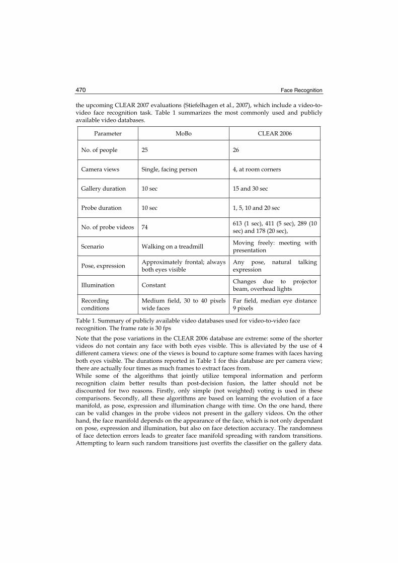
Face Recognition 470
the upcoming CLEAR 2007 evaluations (Stiefelhagen et al., 2007), which include a video-to-video face recognition task. Table 1 summarizes the most commonly used and publicly available video databases.
Parameter MoBo CLEAR 2006
No. of people 25 26
Camera views Single, facing person 4, at room corners
Gallery duration 10 sec 15 and 30 sec
Probe duration 10 sec 1, 5, 10 and 20 sec
No. of probe videos 74 613 (1 sec), 411 (5 sec), 289 (10 sec) and 178 (20 sec),
Scenario Walking on a treadmill Moving freely: meeting with presentation
Pose, expression Approximately frontal; always both eyes visible
Any pose, natural talking expression
Illumination Constant Changes due to projector beam, overhead lights
Recordingconditions
Medium field, 30 to 40 pixels wide faces
Far field, median eye distance 9 pixels
Table 1. Summary of publicly available video databases used for video-to-video face recognition. The frame rate is 30 fps
Note that the pose variations in the CLEAR 2006 database are extreme: some of the shorter videos do not contain any face with both eyes visible. This is alleviated by the use of 4 different camera views: one of the views is bound to capture some frames with faces having both eyes visible. The durations reported in Table 1 for this database are per camera view; there are actually four times as much frames to extract faces from. While some of the algorithms that jointly utilize temporal information and perform recognition claim better results than post-decision fusion, the latter should not be discounted for two reasons. Firstly, only simple (not weighted) voting is used in these comparisons. Secondly, all these algorithms are based on learning the evolution of a face manifold, as pose, expression and illumination change with time. On the one hand, there can be valid changes in the probe videos not present in the gallery videos. On the other hand, the face manifold depends on the appearance of the face, which is not only dependant on pose, expression and illumination, but also on face detection accuracy. The randomness of face detection errors leads to greater face manifold spreading with random transitions. Attempting to learn such random transitions just overfits the classifier on the gallery data.

Far-Field, Multi-Camera, Video-to-Video Face Recognition 471
The effect of these errors is even more pronounced on far-field viewing conditions and unconstrained people movement, where face detection is much harder. All these algorithms have not been tested on such videos. For this reason, we have chosen the post-decision fusion scheme in (Stergiou et al., 2006) for the far-field, unconstrained video-to-video face recognition system detailed in the next section.
3. Proposed face recognition system
In this section we analyze the different options for video-to-video face recognition using the CLEAR 2006 database. We present different solutions for all the detection and recognition subtasks and we investigate their effect on recognition rate. For the reasons discussed in section 2 we choose a post-decision fusion scheme to utilize the temporal information in the video streams.
3.1 Face detection for gallery and probe generation
The CLEAR 2006 database comes with a set of annotations (Stiefelhagen et al., 2007). The face bounding box is marked every 1sec, while the centers of the eyes every 200ms. The lower frequency of the face annotations is due to the severe difficulty of this kind f annotation. Hence the first option for face detection is to simply use these labels to extract the faces. The labels are linearly interpolated to provide the eyes of the person in each frame. Should two eyes exist, the face is cropped, normalized and added to the probe or gallery. Normalization accounts for face geometry and illumination changes. First the marked eyes are positioned on specific coordinates on a 34 by 42 template that contains mostly the face for approximately frontal views of the people. This is a big template for most of the faces; it is selected to favor upsampling of the small faces to downsampling of the large ones. No deliberate perturbation of the eye positions is carried out to alleviate the effect of eye labeling errors (Lee et al., 2003; Ekenel and Pnevmatikakis, 2006). Such an approach is very important for small galleries, and has been applied in the past on still-to-video face recognition on data similar to those of the CLEAR2006 (Ekenel and Pnevmatikakis, 2006), but the rich gallery of this dataset is enough to randomize the errors and alleviate their effect. Then the intensity is made zero-mean, unit variance. Although more aggressive normalization techniques exist to account for illumination changes (Pnevmatikakis & Polymenakos, 2005), these also degrade performance under pose and expression changes (Pnevmatikakis & Polymenakos, 2005). Hence the mild normalization approach is taken here, to provide some immunity to illumination changes without degrading performance under pose changes too much. The normalized gallery images extracted for one person are shown in Figure 1. Evidently there are problems with the accuracy of the interpolated labels, or the 200 ms labels themselves, that lead to scaling errors, shifting and rotation of the faces. Such effects can be from minor up to major, leading to image segments that are definitely not faces (end of row four, beginning of row five). Also, there are pose variations, both left-right (even extreme profile with only one eye visible – row five) and up-down. Finally note the large resolution changes; there are faces where details are visible, and others that are a blur due to the upsampling to bring them to a standard size (contrast the level of detail in the two last rows). The gross resolution variation present in the probe videos is apparent in the histogram of eye distances shown in Figure 2.

Face Recognition 472
Figure 1. Gallery faces cropped from the 15 sec gallery videos, using all four cameras, for one person
100
101
102
0
0.5
1
1.5
2
2.5x 10
4
Eye distance (pixels)
His
togra
m
Figure 2. Histogram of the eye distances of the faces segmented from the probe videos using the manual annotations. The video-to-video face recognition system has to cope with eye distances of 4 to 28 pixels

Far-Field, Multi-Camera, Video-to-Video Face Recognition 473
When the view is not approximately frontal, then the template might include other parts of the head, or even background. Such views are not wanted, and some means for automatically discarding them is needed. Note at this point that automatic selection of faces is a prerequisite only for the probe videos. But it is not only cumbersome to manually filter the gallery stills; such a selection can cause mismatches between the automatically selected probe stills and the manually selected gallery stills. For both these reasons an automatic mechanism for the selection of faces is utilized. This mechanism employs a measure of frontality, based on the supplied face bounding boxes and eye positions. Frontal views should have both eyes symmetrically positioned around the vertical face axis. This symmetry is enumerated in the frontality measure. The measure can unfortunately be inaccurate for two reasons. The first has to do with the provided label files: eye positions are provided every 200 ms, while face bounding boxes every 1 sec, causing larger errors due to interpolation. The second reason has to do with the positioning of the head: when it is not upright, then the major axis of the face does not coincide with the central vertical axis of the face bounding box. Nevertheless, employing the proposed frontality measure rids the system from most of the non-frontal faces at the expense of missing some frontal but tilted ones. As for the threshold on frontality, this should not be too strict to diminish the training and testing data. It is set to 0.1 for all training durations and testing durations up to 10 sec. For testing durations of 20 sec, it is doubled, as the abundance of images in this case allows for a stricter threshold. A final problem with the application of the frontality threshold is that there are some testing segments for which both eyes are never visible. This leads to empty segments. These profile faces can in principle be classified by face recognizers trained on profile faces, but such classifiers have not been implemented in the scope of these experiments. The still gallery and probe sets generated using the face annotations are summarized in Table 2.
Face cropping method Interpolated hand-annotated eye centers Viola-Jones detector
Face normalization De-rotation using the eye centers, scaling to 42 by 34 pixels
No de-rotation, scaling to 48 by 36 pixels
Length (sec) 15 30 15 30 Min 47 56 118 251 Average 241 517 428 886
Gallery stills per person
Max 613 1213 890 1696 Length (sec) 1 5 10 20 1 5 10 20 Min 0 0 0 0 1 2 19 81 Average 16 78 148 301 25 127 226 515 Max 60 282 479 930 90 348 793 1406
Probestills per video
Empty videos 13% 3.4% 1.7% 1.1% 0 0 0 0
Table 2. Summary of the gallery and probe still sets generated from the CLEAR 2006 videos using either the provided face annotations or the trained cascaded detector
Basing the gallery and probe generation of video-to-video face recognition on annotations is not good practice. Annotations and expensive and inaccurate, both because it is difficult to label facial features on far-field recordings, and because interpolation is needed, as the

Face Recognition 474
frames are annotated sparsely. Also, actual systems have to be fully automatic. Hence a face detector is needed. As multiple people are present in the frames, and the faces are tiny compared to the frame size, the natural choice for a detector is the boosted cascade of simple features (Viola and Jones, 2001). Although many improvements on the original algorithm have been proposed (Li and Zhang, 2004; Schneiderman, 2004), we opted to stick to the original version that uses AdaBoost and its implementation in OpenCV (Bradski, 2005), as this is publicly available. Although a trained cascade of simple classifiers is already provided with OpenCV, it is not suitable for our needs as the faces in our far-field recordings are too small. That detector has very high miss rate. A more suitable detector is thus trained. To do so we use 6,000 positive samples (images with marked faces), 20,000 negative samples (images with no human or animal face present), an aspect ratio of 3/4, minimum feature size 0, 99.9% hit rate, 50% false alarm, tilted features, non-symmetric faces and gentle AdaBoost learning (Bradski, 2005). We run the cascaded classifier on all the frames of the gallery and probe videos, and we collect the faces. Note that due to the existence of many people in the frames, the labels are still needed to tell apart the person under consideration from the other meeting participants. If any detection exists close to the provided face bounding box, then it is selected as the face of interest. The temporally subsampled gallery images for the same person shown in Figure 1 are shown in Figure 3.
Figure 3. Temporally subsampled gallery faces automatically cropped from the 15 sec gallery videos, using all four cameras, for one person

Far-Field, Multi-Camera, Video-to-Video Face Recognition 475
Comparing the faces in Figure 1 and 3, it is evident that using the automatic detection scheme we get more faces, but less accurately framed than with the face annotations. Also, there is no attempt to geometrically normalize the faces based on the eye positions, nor any filtering of profile faces. The statistics of the automatically extracted gallery and probe stills are also shown in Table 2.
3.2 Classification
For classification the gallery faces are vectorized by rearranging the intensities of their pixels into a vector, e.g. by reading the intensities in a column-wise fashion. The mean vector is subtracted, yielding zero-mean vectors, to be used for the training of the classifiers. The classifiers employed are of the linear subspace projection family. Both Principal Components Analysis (PCA) (Turk and Pentland, 1991) and Linear Discriminant Analysis (LDA) (Belhumeur et al., 1997) are employed to build unsupervised and supervised projection matrices respectively. PCA aims at transforming the training vectors so that their projections in lower-dimensional spaces has maximum scatter. This guarantees optimality in terms of minimum squared error of the representation of the original vectors in any lower-dimensional space (Duda et al., 2000). The determination of the transformation matrix does not require any class information, hence it is unsupervised. Although the optimality in representation does not offer any guarantee for optimality in classification, the use of PCA has led to the successful Eigenface face recognition method (Turk and Pentland, 1991). The dimension D of the recognition subspace onto which the training vectors are projected is a parameter of the method, to be determined empirically. Suppressing some of the dimensions along which the scatter of the projected vectors is smallest not only increases the speed of the classification, but also seems to be suppressing variability that is irrelevant to the recognition, leading to increased performance. LDA on the other hand aims at maximizing the between-class scatter under the constraint of minimum within-class scatter of the training vectors, effectively minimizing the volume of each class in the recognition space, while maximizing the distance between the classes (Duda et al., 2000). The dimensions of the LDA subspace is − 1K , where K is the number of classes. The determination o the LDA projection matrix requires class information, hence it is supervised. LDA suffers from ill-training (Martinez and Kak, 2001), when the training vectors do not represent well the scatter of the various classes. Nevertheless, given sufficient training, its use in the Fisherfaces method (Belhumeur et al., 1997) has led to very good results. LDA is better for large faces with accurate eye labels (Rentzeperis et al., 2006), but PCA is more robust as face size and eye labeling accuracy drop. LDA is robust to illumination changes (Belhumeur et al., 1997). PCA can be made more robust to illumination changes if some of the eigenvectors corresponding to the largest eigenvalues are excluded from the projection matrix, but this reduces the robustness of PCA under eye misalignment errors. At far-field viewing conditions, resolution is low and the accurate determination of the eye position is very difficult, even for human annotators. To demonstrate the difficulties the far-field viewing conditions impose on face recognition, a comparison of the error rate of PCA, PCA without the three eigenvectors correspond=ding to the three largest eigenvalues (PCA w/o 3) and LDA is carried out in Figure 4, for different face resolutions and eye alignment accuracies. Note that the database used for these experiments is not the video database of CLEAR 2006, but HumanScan (Jesorsky et al., 2001) that offers very large faces which can be
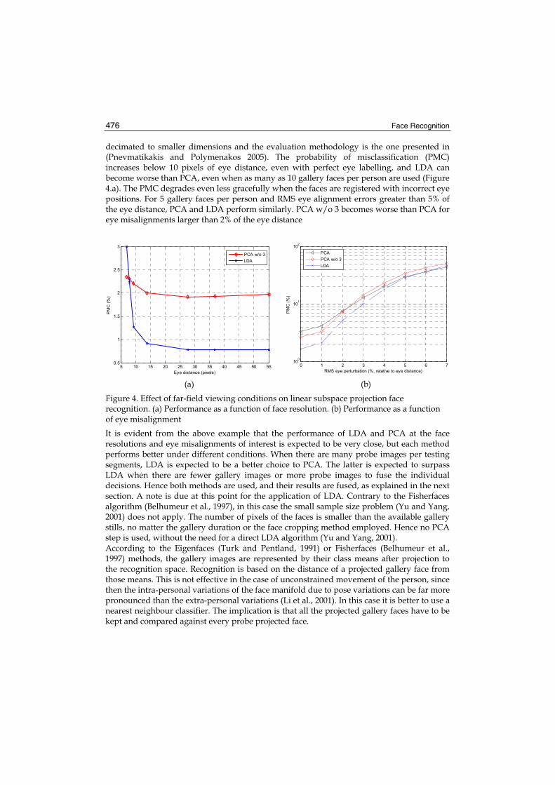
Face Recognition 476
decimated to smaller dimensions and the evaluation methodology is the one presented in (Pnevmatikakis and Polymenakos 2005). The probability of misclassification (PMC) increases below 10 pixels of eye distance, even with perfect eye labelling, and LDA can become worse than PCA, even when as many as 10 gallery faces per person are used (Figure 4.a). The PMC degrades even less gracefully when the faces are registered with incorrect eye positions. For 5 gallery faces per person and RMS eye alignment errors greater than 5% of the eye distance, PCA and LDA perform similarly. PCA w/o 3 becomes worse than PCA for eye misalignments larger than 2% of the eye distance
0 1 2 3 4 5 6 710
0
101
102
RMS eye perturbation (%, relative to eye distance)
PM
C (
%)
PCA
PCA w/o 3
LDA
(a) (b)
Figure 4. Effect of far-field viewing conditions on linear subspace projection face recognition. (a) Performance as a function of face resolution. (b) Performance as a function of eye misalignment
It is evident from the above example that the performance of LDA and PCA at the face resolutions and eye misalignments of interest is expected to be very close, but each method performs better under different conditions. When there are many probe images per testing segments, LDA is expected to be a better choice to PCA. The latter is expected to surpass LDA when there are fewer gallery images or more probe images to fuse the individual decisions. Hence both methods are used, and their results are fused, as explained in the next section. A note is due at this point for the application of LDA. Contrary to the Fisherfaces algorithm (Belhumeur et al., 1997), in this case the small sample size problem (Yu and Yang, 2001) does not apply. The number of pixels of the faces is smaller than the available gallery stills, no matter the gallery duration or the face cropping method employed. Hence no PCA step is used, without the need for a direct LDA algorithm (Yu and Yang, 2001). According to the Eigenfaces (Turk and Pentland, 1991) or Fisherfaces (Belhumeur et al., 1997) methods, the gallery images are represented by their class means after projection to the recognition space. Recognition is based on the distance of a projected gallery face from those means. This is not effective in the case of unconstrained movement of the person, since then the intra-personal variations of the face manifold due to pose variations can be far more pronounced than the extra-personal variations (Li et al., 2001). In this case it is better to use a nearest neighbour classifier. The implication is that all the projected gallery faces have to be kept and compared against every probe projected face.
5 10 15 20 25 30 35 40 45 50 550.5
1
1.5
2
2.5
3
Eye distance (pixels)
PM
C (
%)
PCA w/o 3
LDA
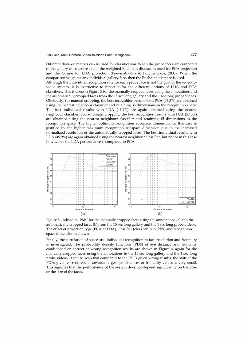
Far-Field, Multi-Camera, Video-to-Video Face Recognition 477
Different distance metrics can be used for classification. When the probe faces are compared to the gallery class centres, then the weighted Euclidian distance is used for PCA projection and the Cosine for LDA projection (Pnevmatikakis & Polymenakos, 2005). When the comparison is against any individual gallery face, then the Euclidian distance is used. Although the individual recognition rate for each probe face is not the goal of the video-to-video system, it is instructive to report it for the different options of LDA and PCA classifiers. This is done in Figure 5 for the manually cropped faces using the annotations and the automatically cropped faces from the 15 sec long gallery and the 1 sec long probe videos. Obviously, for manual cropping, the best recognition results with PCA (46.5%) are obtained using the nearest neighbour classifier and retaining 35 dimensions in the recognition space. The best individual results with LDA (44.1%) are again obtained using the nearest neighbour classifier. For automatic cropping, the best recognition results with PCA (57.5%) are obtained using the nearest neighbour classifier and retaining 45 dimensions in the recognition space. The higher optimum recognition subspace dimension for this case is justified by the higher maximum recognition subspace dimension due to the increased normalized resolution of the automatically cropped faces. The best individual results with LDA (49.9%) are again obtained using the nearest neighbour classifier, but notice in this case how worse the LDA performance is compared to PCA.
101
102
103
38
39
40
41
42
43
44
45
46
47
Indiv
idual re
cognitio
n r
ate
(%
)
Subspace dimensions
PCA center
PCA NN
LDA center
LDA NN
101
102
103
49
50
51
52
53
54
55
56
57
58
Indiv
idual re
cognitio
n r
ate
(%
)
Subspace dimensions
PCA NN
LDA NN
(a) (b)
Figure 5. Individual PMC for the manually cropped faces using the annotations (a) and the automatically cropped faces (b) from the 15 sec long gallery and the 1 sec long probe videos. The effect of projection type (PCA or LDA), classifier (class centre or NN) and recognition space dimension is shown
Finally, the correlation of successful individual recognition to face resolution and frontality is investigated. The probability density functions (PDF) of eye distance and frontality conditioned on correct or wrong recognition results are shown in Figure 6, again for the manually cropped faces using the annotations in the 15 sec long gallery and the 1 sec long probe videos. It can be seen that compared to the PDFs given wrong results, the shift of the PDFs given correct results towards larger eye distances or frontality values is very small. This signifies that the performance of the system does not depend significantly on the pose or the size of the faces.
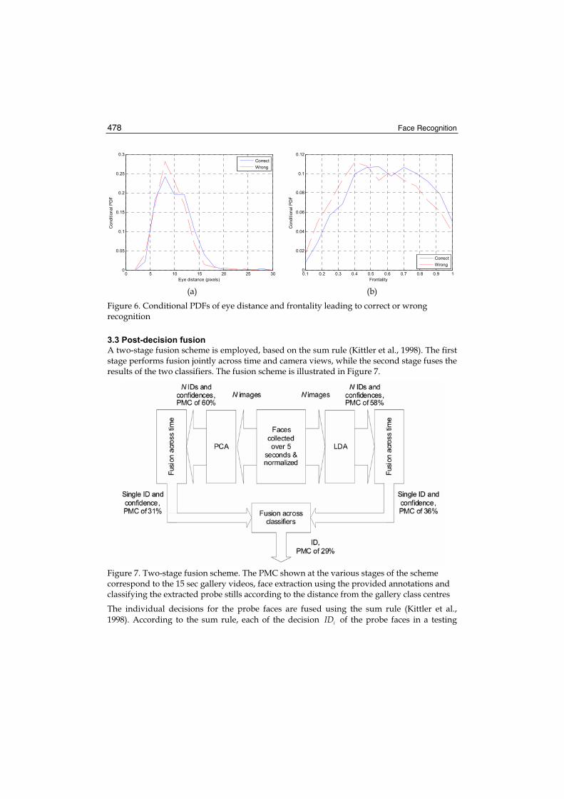
Face Recognition 478
0 5 10 15 20 25 300
0.05
0.1
0.15
0.2
0.25
0.3
Eye distance (pixels)
Conditio
nal P
DF
Correct
Wrong
0.1 0.2 0.3 0.4 0.5 0.6 0.7 0.8 0.9 10
0.02
0.04
0.06
0.08
0.1
0.12
Frontality
Conditio
nal P
DF
Correct
Wrong
(a) (b)
Figure 6. Conditional PDFs of eye distance and frontality leading to correct or wrong recognition
3.3 Post-decision fusion
A two-stage fusion scheme is employed, based on the sum rule (Kittler et al., 1998). The first stage performs fusion jointly across time and camera views, while the second stage fuses the results of the two classifiers. The fusion scheme is illustrated in Figure 7.
Figure 7. Two-stage fusion scheme. The PMC shown at the various stages of the scheme correspond to the 15 sec gallery videos, face extraction using the provided annotations and classifying the extracted probe stills according to the distance from the gallery class centres
The individual decisions for the probe faces are fused using the sum rule (Kittler et al., 1998). According to the sum rule, each of the decision iID of the probe faces in a testing

Far-Field, Multi-Camera, Video-to-Video Face Recognition 479
segment casts a vote that carries a weight iw . The weights iw of every decision such as =iID k are summed to yield the weights kW of each class:
=
=: i
k ii ID k
W w (1)
where = 1, ,k K and K is the number of classes. Then the fused decision based on the Nindividual identities is:
( ) ( )= arg maxNk
kID W (2)
The weight iw in the sum rule for the i-th decision is the sixth power of the ratio of the second-minimum distance (1)
id over the minimum distance (1)id :
=6(2)
(1)i
ii
dwd
(3)
This choice for weight reflects the classification confidence: If the two smallest distances from the class centers are approximately equal, then the selection of the identity leading to the smallest distance is unreliable. In this case the weight is close to unity, weighting down the particular decision. If on the other hand the minimum distance is much smaller than the second-minimum, the decision is heavily weighted as the selection of the identity is reliable. The sixth power allows for a few very confident decisions to be weighted more then many less confident ones. The suitability of the proposed weights is demonstrated in Figure 8, where the conditional cumulative density functions (CDF) of the weights, conditioned on correct or wrong recognition are shown for the manually cropped faces using the annotations and the automatic detection scheme, in the 15 sec long gallery and the 1 sec long probe videos. It is evident from Figure 8 that the probability of wrong recognition diminishes as the proposed weight increases, hence they can be used in a weighted voting scheme. The fused recognition rate of PCA increases from the 71.7% obtained by majority voting, to 72.8% obtained by using the proposed weighted voting scheme. Also, the weights for the faces cropped using the automatic detection scheme are more suitable than those of the manual: The CDFs given wrong decisions are practically the same, while the CDF given correct decisions for the automatic scheme is shifted to larger weights compared to that for manual cropping. Hence, not only the individual recognition rates for the automatic scheme are higher (see Figure 5), but in addition it is expected that the gain due to fusion will be higher. Indeed, fusing the individual PCA results on the manually cropped probes from the 1 sec long videos, we obtain a recognition rate of 53.8%, with a relative increase from the individual rate of 15.7%. On the other hand, fusing the individual PCA results on the automatically cropped probes, we obtain a recognition rate of 72.8%, with a relative increase from the individual rate of 26.5%. The decisions ( )PCAID and ( )LDAID of the PCA and the LDA classifiers are again fused using the sum rule to yield the reported identity. For this fusion, the class weights kW of equation (1) are used instead of the distances in equation (3). Setting:

Face Recognition 480
[ ] ( )
[ ]≡ =≡
1
2
best matching classsecond-best matching class
Nk IDk
(4)
the weights of the PCA and LDA decisions become:
= 1
2
( )
( )
ik
i ik
Ww
W, { }∈ PCA, LDAi (5)
Then the fused PCA/LDA decision is:
( )
( )
≥=
<
PCAPCA LDA
LDAPCA LDA
if
if
ID w wID
ID w w (6)
100
101
0
0.1
0.2
0.3
0.4
0.5
0.6
0.7
0.8
0.9
1
Weight
Conditio
nal P
DF
Correct, manual
Correct, VJ
Wrong, manual
Wrong, VJ
Figure 8. Conditional cumulative density functions of the weights, conditioned on correct or wrong recognition are shown for the manually cropped faces using the annotations and the automatic detection scheme, in the 15 sec long gallery and the 1 sec long probe videos. The weights from the PCA classifier are used
3.4 Performance
The performance of the video-to-video face recognition system described in this section is presented next. This system using the manual annotations for gallery and probe still generation and classification based on the distance from projected gallery class centres has been evaluated in CLEAR 2006. Performance can be significantly boosted using the nearest neighbour classifier, especially for the 30 sec long gallery videos. An even greater
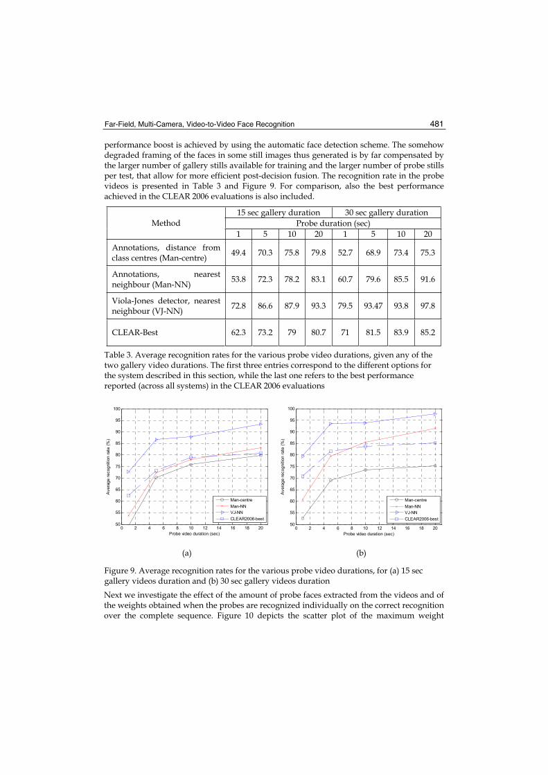
Far-Field, Multi-Camera, Video-to-Video Face Recognition 481
performance boost is achieved by using the automatic face detection scheme. The somehow degraded framing of the faces in some still images thus generated is by far compensated by the larger number of gallery stills available for training and the larger number of probe stills per test, that allow for more efficient post-decision fusion. The recognition rate in the probe videos is presented in Table 3 and Figure 9. For comparison, also the best performance achieved in the CLEAR 2006 evaluations is also included.
15 sec gallery duration 30 sec gallery duration Probe duration (sec) Method
1 5 10 20 1 5 10 20 Annotations, distance from class centres (Man-centre) 49.4 70.3 75.8 79.8 52.7 68.9 73.4 75.3
Annotations, nearest neighbour (Man-NN) 53.8 72.3 78.2 83.1 60.7 79.6 85.5 91.6
Viola-Jones detector, nearest neighbour (VJ-NN) 72.8 86.6 87.9 93.3 79.5 93.47 93.8 97.8
CLEAR-Best 62.3 73.2 79 80.7 71 81.5 83.9 85.2
Table 3. Average recognition rates for the various probe video durations, given any of the two gallery video durations. The first three entries correspond to the different options for the system described in this section, while the last one refers to the best performance reported (across all systems) in the CLEAR 2006 evaluations
0 2 4 6 8 10 12 14 16 18 2050
55
60
65
70
75
80
85
90
95
100
Probe video duration (sec)
Avera
ge r
ecognitio
n r
ate
(%
)
Man-centre
Man-NN
VJ-NN
CLEAR2006-best
0 2 4 6 8 10 12 14 16 18 2050
55
60
65
70
75
80
85
90
95
100
Probe video duration (sec)
Avera
ge r
ecognitio
n r
ate
(%
)
Man-centre
Man-NN
VJ-NN
CLEAR2006-best
(a) (b)
Figure 9. Average recognition rates for the various probe video durations, for (a) 15 sec gallery videos duration and (b) 30 sec gallery videos duration
Next we investigate the effect of the amount of probe faces extracted from the videos and of the weights obtained when the probes are recognized individually on the correct recognition over the complete sequence. Figure 10 depicts the scatter plot of the maximum weight
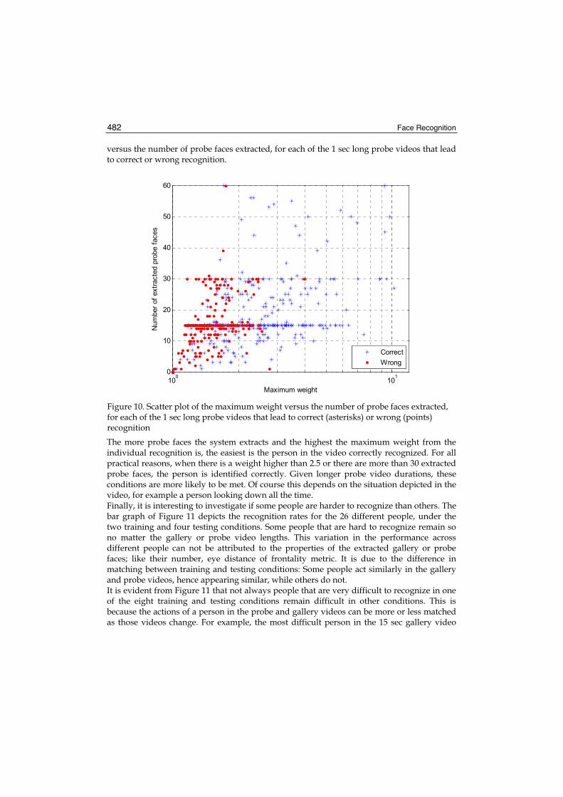
Face Recognition 482
versus the number of probe faces extracted, for each of the 1 sec long probe videos that lead to correct or wrong recognition.
100
101
0
10
20
30
40
50
60
Maximum weight
Num
ber
of
extr
acte
d p
robe f
aces
Correct
Wrong
Figure 10. Scatter plot of the maximum weight versus the number of probe faces extracted, for each of the 1 sec long probe videos that lead to correct (asterisks) or wrong (points) recognition
The more probe faces the system extracts and the highest the maximum weight from the individual recognition is, the easiest is the person in the video correctly recognized. For all practical reasons, when there is a weight higher than 2.5 or there are more than 30 extracted probe faces, the person is identified correctly. Given longer probe video durations, these conditions are more likely to be met. Of course this depends on the situation depicted in the video, for example a person looking down all the time. Finally, it is interesting to investigate if some people are harder to recognize than others. The bar graph of Figure 11 depicts the recognition rates for the 26 different people, under the two training and four testing conditions. Some people that are hard to recognize remain so no matter the gallery or probe video lengths. This variation in the performance across different people can not be attributed to the properties of the extracted gallery or probe faces; like their number, eye distance of frontality metric. It is due to the difference in matching between training and testing conditions: Some people act similarly in the gallery and probe videos, hence appearing similar, while others do not. It is evident from Figure 11 that not always people that are very difficult to recognize in one of the eight training and testing conditions remain difficult in other conditions. This is because the actions of a person in the probe and gallery videos can be more or less matched as those videos change. For example, the most difficult person in the 15 sec gallery video

Far-Field, Multi-Camera, Video-to-Video Face Recognition 483
and 1 sec probe videos, is easier than people 2 and 7 in the 10 sec probe videos, and easier than people 2-6, 8, 10 and 14 in the 30 sec gallery video.
0 5 10 15 20 2530
40
50
60
70
80
90
100
Person no.
Recognitio
n r
ate
(%
)
(a)
0 5 10 15 20 2530
40
50
60
70
80
90
100
Person no.
Recognitio
n r
ate
(%
)
(b)Figure 11. Per person recognition rates for the different durations of the probe videos (grouped) and for the 15 sec (a) or 30 sec (b) long gallery videos. The people are sorted by ascending recognition rate for the 1 sec long probe and the 15 sec long gallery videos
Finally, there is a large deviation in recognition performance in the 15 sec gallery video and 1 sec probe videos. This drops somewhat for longer probe and gallery videos. This is demonstrated in Figure 12, where the standard deviation of the recognition rate across the 26 different people is depicted for the four probe video durations and the two gallery video durations. Hence increasing the probe or gallery durations tend to make performance across different people both better and more uniform.

Face Recognition 484
0 2 4 6 8 10 12 14 16 18 204
6
8
10
12
14
16
18
Probe video duration (sec)
Sta
ndard
devia
tion o
f re
cognitio
n r
ate
acro
ss p
eople
15 sec gallery
30 sec gallery
Figure 12. Standard deviation of the recognition rate across the 26 different people for the four probe video durations and the two gallery video durations. Performance across the different people is more uniform as the durations increase
4. Conclusion and possible extensions
In this chapter we have presented the tradeoffs in video-to-video face recognition, applied on far-field, unconstrained recordings. We have demonstrated that given long probe video durations the performance of a system based on a frontal Viola-Jones face detector, linear subspace projection and nearest neighbour classifier more or less solves the problem, with average recognition rates above 95%. In applications where long probe videos are impractical, performance is still low (recognition rates of 74% or 80% for 1 sec probe and 15 sec or 30 sec gallery video durations), especially given that the number of people are limited to the modest number of 26. To further enhance performance, there are some possible system enhancements: • Multiple face detectors can be trained, including poses other than frontal. Also, face
detection can be coupled with a probabilistic tracker based on particle filtering (Zhou et al., 2004) or a deterministic tracker based on colour histograms using CAMShift (Bradski, 1998). This will provide more stills, capturing more pose variations.
• Other distance metrics (weighted Euclidian, cosine) can be used for nearest neighbour classification.
• Modelling of face sequences, similar to the exemplar approach of (Zhou et al., 2003), to automatically detect outliers that are not smooth pose transitions, but rather face detector errors. The cleaner face sequences thus obtained can be used to model pose transitions, allowing more efficient utilization of temporal information than weighted voting (Weng et al., 2000; Li et al., 2001; Lee et al., 2003; Liu and Chen, 2003; Aggarval et al., 2004).

Far-Field, Multi-Camera, Video-to-Video Face Recognition 485
5. Acknowledgements
This work is sponsored by the European Union under the integrated project CHIL, contract number 506909.
6. References
Aggarwal, G.; Roy-Chowdhury, A.K. & Chellappa, R. (2004). A System Identification Approach for Video-based Face Recognition, Proceedings of International Conference on Pattern Recognition, Cambridge, UK, Aug. 2004
Belhumeur, P.; Hespanha, J. & Kriegman, D. (1997). Eigenfaces vs. Fisherfaces: Recognition Using Class Specific Linear Projection. IEEE Transactions on Pattern Analysis and Machine Intelligence, 19, 7, 711-720
Bradski, G. (1998). Computer Vision Face Tracking for Use in a Perceptual User Interface. Intel Technology Journal, 2
Bradski, G.; Kaehler, A. & Pisarevsky, V. (2005). Learning-Based Computer Vision with Intel's Open Source Computer Vision Library. Intel Technology Journal, 9
Duda, R.; Hart, P. & Stork, D. (2000). Pattern Classification. Wiley-Interscience, New York Ekenel, H. & Pnevmatikakis, A. (2006). Video-Based Face Recognition Evaluation in the
CHIL Project – Run 1, Proceedings of IEEE Conference on Automatic Face and Gesture Recognition, pp. 85-90, Southampton, UK, Apr., 2006
Gorodnichi, D. (2003). Facial Recognition in Video. In: AVBPA 2003, Lecture Notes in Computer Science 2688, Kittler, J. & Nixon, M.S. (Ed.), 505-514, Springer-Verlag, Berlin Heidelberg
Jesorsky, O.; Kirchberg, K. & Frischholz, R. (2001). Robust Face Detection Using the Hausdorff Distance. In Bigun, J. & Smeraldi, F. (ed.), Audio and Video based Person Authentication, 90-95, Springer-Verlag, Berlin Heidelberg
Kittler, J.; Hatef, M.; Duin, R.P.W. & Matas, J. (1998). On combining classifiers. IEEE Transactions on Pattern Analysis and Machine Intelligence, 20, 3, 226–239
Lee, K.-C..; Ho, J.; Yang, M.-H. & Kriegman, D. (2003). Video-based face recognition using probabilistic appearance manifolds. Proceedings of IEEE Conference on Computer Vision and Pattern Recognition, 1, pp. 313-320, Madison, Wisconsin, USA, June 2003
Li, Y.; Gong, S. & Liddell, H. (2001). Video-Based Online Face Recognition Using Identity Surfaces. Proceedings of IEEE ICCV Workshop on Recognition, Analysis, and Tracking of Faces and Gestures in Real-Time Systems, pp. 40-46, Vancouver, Canada, July 2001
Li, S.-Z. & Zhang, Z.Q. (2004). FloatBoost Learning and Statistical Face Detection. IEEETransactions on Pattern Analysis and Machine Intelligence, 26, 9, 1112-1123
Liu, X.. & Chen, T. (2003). Video-based face recognition using adaptive hidden markov models. Proceedings of IEEE Conference on Computer Vision and Pattern Recognition, 1,pp. 340-345, Madison, Wisconsin, USA, June 2003
Martínez , A. & Kak, A. (2001). PCA versus LDA. IEEE Transactions on Pattern Analysis and Machine Intelligence, 23, 2, 228-233
Phillips, J.; Flynn, P.; Scruggs, T.; Boyer, K. & Worek, W. (2006). Preliminary Face Recognition Grand Challenge Results. Proceedings of IEEE Conference on Automatic Face and Gesture Recognition, pp. 15-21, Southampton, UK, Apr., 2006

Face Recognition 486
Pnevmatikakis, A. & Polymenakos, L. (2005). A testing methodology for face recognition algorithms. In: MLMI 2005, Lecture Notes in Computer Science 3869, Renals, S. & Bengio, S. (Ed.), 218-229, Springer-Verlag, Berlin Heidelberg
Raytchev, B. & Murase, H. (2003). Unsupervised recognition of multi-view face sequences based on pairwise clustering with attraction and repulsion. Computer Vision and Image Understanding, 91, 22-52
Rentzeperis, E.; Stergiou, A.; Pnevmatikakis, A. & Polymenakos, L. (2006). Impact of Face Registration Errors on Recognition. Artificial Intelligence Applications and Innovations,Peania, Greece, June 2006
Schneiderman, H. (2004). Feature-Centric Evaluation for Efficient Cascaded Object Detection. Proceedings of IEEE Conference on Computer Vision and Pattern Recognition,Washington, DC, USA, June 2004
Stergiou, A.; Pnevmatikakis, A. & Polymenakos, L. (2007). A Decision Fusion System across Time and Classifiers for Audio-visual Person Identification. In: CLEAR 2006, Lecture Notes in Computer Science 4122, Stiefelhagen, R. & Garofolo, J. (Ed.), 218-229, Springer-Verlag, Berlin Heidelberg
Stiefelhagen, R.; Bernardin, K., Bowers, R., Garofolo, J., Mostefa, D. & Soundararajan, P. (2007). The CLEAR 2006 Evaluation. In: CLEAR 2006, Lecture Notes in Computer Science 4122, Stiefelhagen, R. & Garofolo, J. (Ed.), 218-229, Springer-Verlag, Berlin Heidelberg
Turk, M. & Pentland, A. (1991). Eigenfaces for Recognition. J. Cognitive Neuroscience, 3, 71-86 Viola, P. & Jones, M. (2001). Rapid Object Detection using a Boosted Cascade of Simple
Features. Proceedings of IEEE Conference on Computer Vision and Pattern Recognition,p. 511, Hawaii, Dec. 2001
Waibel, A.; Steusloff, H. & Stiefelhagen, R. (2004). CHIL: Computers in the Human Interaction Loop, 5th International Workshop on Image Analysis for Multimedia Interactive Services, Lisboa, Portugal, April 21-23, 2004
Weng, J.; Evans, C.H. & Hwang, W.-S. (2000). An Incremental Learning Method for Face Recognition under Continuous Video Stream. Proceedings of IEEE Conference on Automatic Face and Gesture Recognition, pp. 251-256, Grenoble, France, March 2000
Xie, C.; Vijaya Kumar, B. V. K.; Palanivel, S. & B. Yegnanarayana (2004). A Still-to-Video Face Verification System Using Advanced Correlation Filters. In: ICBA 2004, Lecture Notes in Computer Science 3072, Zhang, D. & Jain, A.K. (Ed.), 102-108, Springer-Verlag, Berlin Heidelberg
Yu, H. & Yang, J. (2001). A direct LDA algorithm for high-dimensional data with application to face recognition. Pattern Recognition, 34, 2067–2070
Zhou, S.; Krueger, V. & Chellappa, R. (2003). Probabilistic recognition of human faces from video. Computer Vision and Image Understanding, 91, 7, 214-245
Zhou, S.; Chellappa, R. & Moghaddam, B. (2004). Visual tracking and recognition using appearance-adaptive models in particle filters. IEEE Transactions on Image Processing, 13, 11, 1491-1506
25
Facing Visual Tasks Based on Different Cognitive Architectures
Marcos Ruiz-Soler and Francesc S. Beltran Universidad de Málaga and Universitat de Barcelona
Spain
1. Introduction
Today’s technology has produced machines that imitate and even exceed many human abilities. Nobody is surprised when a calculator does highly complex mathematical computations or an electronic chess program beats a renowned chess master. Any computer can store and retrieve detailed information about very different topics and establish a multitude of complex relations. However, in spite of recent spectacular advances, robotics has not yet been able to reproduce with the same efficiency some basic tasks every human being can do effortlessly, such as understanding contextual images and moving in complex physical spaces. The apparent simplicity of understanding images and walking may be an obstacle when it comes to judging the real complexity of these tasks. But even now, after many ingenious attempts to solve the problems inherent to these perceptual and motor processes, technology has still not been able to recreate levels similar to those of a human being. We therefore think it is of interest to review what we know about human beings and try to learn about this very efficient biological system. This chapter will examine the results of research on humans to come up with some valuable suggestions for designs of artificial systems for face recognition. We will begin with a quick review of the contributions made in two main areas of face-recognition research in the last thirty years: image properties and perceptual tasks. The analysis of both will lead us to explore some internal characteristics of the system (cognitive architecture) that are not usually considered: the representational format of visual information and kinds of flow processing. Based on these factors, we will make some suggestions about the direction future research efforts should take in the field of face recognition.
2. Looking outside: from image properties to visual tasks
2.1 Image properties and spatial frequencies
Given the fact that any image, whether of a human face or any other visual object, can be described in terms of spatial frequencies (SFs) (i.e. it can be described as the sum of a set of sinusoidal grids with different frequencies and orientations), psychophysical research into contrast detection and adaptation to specific SFs has proven that our perceptual system analyses visual input on multiple scales and frequencies (see De Valois & De Valois, 1988;

Face Recognition 488
Graham, 1989). It is therefore generally agreed that spatial filtering is the basic mechanism for extracting visual information from luminance contrasts in early visual processes (see Legge & Gu, 1989; Marr & Hildreth, 1980; Marshall et al., 1996; and Morgan, 1992). In light of all this, one of the main approaches in face-perception research involves manipulating the SF bands in the luminance spectrum of images and observing how these changes affect the performance of visual tasks. Two main questions were asked when investigating the role of SFs in face perception: (1) What range of SFs is necessary to recognize a face? and (2) in what order are low spatial frequencies (LSFs) and high spatial frequencies (HSFs) integrated in face perception and how does this order affect recognition? Studies done to answer the first question mainly used a masking approach, while studies to answer the second question used a microgeneticapproach. Unfortunately, definitive results were not found because the results obtained to answer the first question showed that an extensive range of SFs seems to play a role in recognition; and the results obtained to answer the second question showed that the order of integration does not always point towards the same length of time or order of integration. The results of the studies designed to determine what range of SFs is necessary to recognize a face indicated that recognition decreases when images contain only SFs below about 8 cycles/fw (between 6 and 9 cycles/fw), and that the elimination of the SF range between 8 and 16 cycles/fw produces greater disruption than the elimination of SFs outside this range. Hence, the information contained in a small medium range of SFs contributes more to the face-recognition process than the information contained in all the other SFs (Costen et al., 1994, 1996; Näsänen, 1999; Parker & Costen, 1999). However, though all these results indicated that privileged information can be found in medium-range SFs, the role of the SFs outside that range should not be overlooked. The same studies that identified the optimal medium range of SFs also showed acceptable performance by subjects when SFs above and below the medium range were used. Images of faces made with SFs centred at 50.15 cycles/fw or 2.46 cycles/fw (which is extraordinarily far from the medium range) showed a recognition efficiency only 15% lower than the efficiency when recognizing images of faces made with medium-range SFs (Parker & Costen, 1999). Moreover, the tails obtained in the sensitivity function for images of faces indicated that an extensive range of SFs contributes to recognition (Näsänen, 1999). Given all these results, the conclusion was reached that the idea of a “critical range” of SFs for face recognition should be replaced with the notion of an “optimal range” of SFs for face recognition: a preferred, but not exclusive, tendency to use the information contained in a given range of SFs. The results of the studies designed to determine in what order low spatial frequencies (LSFs) and high spatial frequencies (HSFs) are integrated in face perception and how this order affects recognition appeared to contradict each other: some favoured the hypothesis of anisotropic integration, whereas others pointed to a third interaction factor that might explain why one order of integration is used instead of another. This factor could be the focus of attention and/or the complexity of the stimulus (Bachmann & Kahusk, 1997; Hoeger, 1997, respectively). In summary, all these results indicated that the critical question for predicting subjects’ performance, after the first integrative stage from LSFs to HSFs, is: which SFs provide the information required to solve the on-going task?

Facing Visual Tasks Based on Different Cognitive Architectures 489
2.2 Visual tasks and face perception
Research into face perception using spatial filtering has shown that one of the aspects most analysed are the physical properties of images. In the masking approach, the spatial effects of face representation were the main ones studied, whereas in the microgenetic approach, the focus was primarily on the temporal effects of face representation. But, as discussed above, no conclusive results were found. This may have been due to the different tasks used in face-perception research. It is therefore necessary to differentiate between them as a first step towards clarifying research results. All of them can easily be grouped into five categories: 1. Detection. This consists of distinguishing between face visual stimuli and similar visual stimuli. A detection task asks the viewer of a visual stimulus: “Is x a face?” (e.g. Kuehn & Jolicoeur, 1994; Purcell et al., 1996). 2. Discrimination. This consists of distinguishing perceptually between pairs of faces, either following a holistic or analytical strategy. A discrimination task asks the following question: “Is x the same face as y?” The level of complexity in this task depends on the level of similarity of the faces compared, one or more components of which are usually manipulated by computer software (such as the eyes, mouth, nose, hair, chin, etc.) or orientation (frontal, profile or ¾). Examples of this can be found in Bradshaw & Wallace (1971) or Sergent (1984). 3. Categorization. This consists of answering the question: “Does this face belong to the category x?” It is a classification with two modalities: automatic and controlled. Automatic categorization involves classifying a face into a well-learned conceptual category, which demands very little effort. Categorization by sex or race belongs to this group. It has been employed in research about perceptual discrimination based on gender (Bruce et al., 1993; Burton et al., 1993; Brown & Perrett, 1993; Bruce & Langton, 1994; Chronicle et al., 1995;) and to study the so-called “race effect”. Controlled categorization involves classifying a face into a major category for the subject’s goals; it is conscientiously carried out and could admit very different levels of complexity. This category can include judgements about facial emotions, dispositional attributions (e.g. he/she looks intelligent) and situational attributions (e.g. she/he looks doubtful). This task has been used in research into social cognition. 4. Recognition. This consists of deciding if a face has been seen before. It is assumed that any known or familiar face will be recognized, and that other faces shown during a controlled projection will also be recognized. Therefore, a task like this demands an answer to the question: “Have you seen face x before?”. 5. Identification. This involves establishing a biunivocal assignation between one face and one specific person. An identification task asks the question: Who does face x belong to? (or simply: “Who is he/she?”). The identification task is usually carried out by naming, but an answer such as “It is the face of the president’s wife” is also a form of identification. This is the most specific form of face perception. From a general perspective, all these tasks can be considered specific cases of categorization, ranging from the broadest category (“It is a face”) to the most specific one (“It is Marc’s face”). Therefore, the cognitive resources required are very different, depending on the level required by the task. As a result, Morrison & Schyns (2001) pointed out that the mechanisms of categorization can modulate the use of different scales, depending on the presence of task-dependent, diagnostic information.

Face Recognition 490
2.3 Interaction between images and tasks: the diagnosticity approach
The varying importance of SFs depending on task demands was described by Schyns (1998). It is well known that one object can be put into different categories, depending on the categorization criteria used. For example, a car can be categorized by trademark, model, power, colour, etc.; and a human face can be categorized by sex, race, expression, attraction, etc. According to Schyns’ proposal, the information required to place the same object in one category or another will change depending on the categorization criterion chosen or, in other words, categorization/recognition processes can be characterized as an interaction of task constraints and object information. Task constraints are related to the information needed to place the perceptual object in the category required by the task. For example, given the question: “Is this object a car?”, it will be necessary to find certain visual information, such as wheels, rear-view mirrors, a steering wheel, etc., before providing an answer. Object information is related to the informative-perceptual structure available for placing the perceptual object in the category demanded by the task. If it is possible to observe wheels, rear-view mirrors, a steering wheel, etc. in the image of the object, the necessary information is available for categorization and to answer the question. Therefore, given a specific perceptual task, a group of visual characteristics of the object becomes particularly useful (diagnostic), since it provides the information required to place the object in the category that resolves the task. Information about objects is organized in categories, which are then organized in a hierarchy where it is possible to distinguish three levels (Rosch et al., 1976): the basic level(e.g. a car or a face), the subordinate level (e.g. a BMW Z8 or Claudia Schiffer) and thesuperordinate level (e.g. a vehicle or a head), where the basic level plays a role of primal access(Biederman, 1987) or entry point (Jolicoeur et al., 1984) in the hierarchical system. The categorization process at the superordinate level requires more functional information than perceptual information, while at the subordinate level it requires supplementary perceptual information. Thus, the subordinate level represents maximum informativity and minimum distinctiveness, while the subordinate level represents maximum distinctiveness and minimum informativity. The basic level is on an intermediate level between informativity and distinctiveness, and this provides a compromise solution between accuracy in categorization at a more general level and predictive power at a more specific level (Murphy & Lassaline, 1998), which explains its critical role as primal access in the hierarchy. Nevertheless, requirements of informativity and distinctiveness are not uniform for every category, but depend on the subject’s level of expertise and history of learning. Therefore, in categorization processes where the subject’s expertise skills are at a maximum, as in the case of face recognition, perceptual cues must be diagnostic for the task (sufficient), they cannot overlap with other categories (unique) and they must have sufficient perceptual salience (significant). Therefore, the information I perceive when I see a face will be very different if I have to recognize the face of someone of a different race among people attending a conference, or if I have to recognize the face of a family member among a group of people, or if I have to recognize my partner’s face in a shopping centre. In the first case, the colour of the skin or the shape of the eyes can be maximally diagnostic, while in the second and third cases, the configurational properties will probably be maximally diagnostic for recognition. Oliva & Schyns (1997) found that when the already integrated early perceptual representation is formed, it may be used flexibly in a top-controlled manner permitting selective use of LSFs or HSFs depending on how “diagnostic” they are for the task. Taking

Facing Visual Tasks Based on Different Cognitive Architectures 491
this into account, although the possible importance of task demands in face perception has been explicitly affirmed by several researchers (e.g., Costen et al., 1996; McSorley & Findlay, 1999; and Sergent, 1986, 1994), we suggest that a key question for determining the role SFs play in face perception is not really which SFs are necessary or in which sequential order they are integrated, but rather how LSFs and HSFs are made use of in face perception depending on the demands of the task involved. Therefore, the role of different SFs is critically modulated by the subject’s visual task and it is only when there is no specific visual task that the mandatory aspects of SF processing work by default. When the results of the research in face perception carried out in the last thirty years are examined from the diagnosticity approach, it is possible to see that some contradictions disappear. And this is due to the fact that the questions “Which SFs are critical?” and “Which SFs are integrated?” lose their meaning in an isolated context and have to be considered within the frame of the demands of the task at hand. The questions must then be transformed into “which SFs are diagnostic for recognition/identification of an image?” (Ruiz-Soler & Beltran, 2006).
3. Looking inside: the importance of the functional cognitive architecture
How can it be explained that the same visual task can be solved using different SFs? The observed fact that certain perceptual tasks can be solved using different SFs (Sergent, 1985) makes it necessary to include another factor to explain these data. We believe that, together with image properties and task demands, we must include another explanatory factor: the subject’s characteristics (observer), characteristics that affect individual differences in two areas: (1) the mental representation for faces (something conditioned by the familiarity level or expertise level in relation to them) and (2) the preferential strategy for visual processing (something conditioned by the subject’s hemispheric dominance or cognitive style). What is the empirical evidence for considering mental representation a new explanatory factor? With regard to mental representation, memory research using faces as stimuli has reported a different codification of them depending on the previous knowledge level (Liu et al., 2000; O’Toole et al., 1992). Moreover, research into experts and novices using stimuli with perceptual characteristics very similar to faces (complex, symmetrical, 3D, intersimilars, etc.) have proved the existence of different mental representations (Coin et al., 1992; Harvey & Sinclair, 1985; Millward & O’Toole, 1986). With regard to the processing strategy, research taking into account hemispheric cerebral dominance (Keenan et al., 1989, 1990 and, in particular, Ivry & Robertson, 1998) can be considered, as well as some other research designed to study the development of expert skills in perceptual discrimination (Gauthier & Tarr, 1997; Gauthier et al., 1998; Gauthier et al., 1999; Gauthier & Logothetis, 2000) and the reinterpretation of data from specific research in visual perception. Results point to processing linked to cognitive styles, where some subjects are basically analytical (field-independence subjects) and others are basically holistic (field-dependence subjects), a circumstance that we could re-conceptualize as subjects who preferentially process HSFs and subjects who preferentially process LSFs. Though some previous studies have not shown the relationships between these two aspects (Bruce, 1998), this is a field that we have begun to explore, after creating some procedure controls, by classifying field-dependence subjects, but not merely as those who are excluded from the group of field-independence subjects, as is usually done (Ruiz-Soler et al., 2000).

Face Recognition 492
4. Looking everywhere: new directions in face-recognition research
In this chapter, we have seen how a great deal of research has shown that image properties and task requirements are two interacting factors. We have also seen that the representational format of the information and the preferential processing mode are relevant factors in face perception. What does all this contribute to the design of artificial face-recognition systems? Looking outside shows that the most important information in an image is none other than the information that is most diagnostic (sufficient, unique and significant) for the task at hand. Looking inside shows that we should probably have several representational formats (based on LSFs and HSFs) and a number of different information systems (coarse-to-fine and fine-to-coarse) to come up with a very flexible, efficient system (at least as flexible and efficient as a human being). Designing systems that access representational formats with fine information or that merely use HSFs to process tasks that do not require such fine information (e.g. detection) means having a very inefficient system because it will use much more processing resources than are strictly necessary. But designing systems that have only one representational format or a single processing mode means losing the possibility of performing many of the tasks inherent to face recognition.
5. References
Bachmann, T. & Kahusk, N. (1997). The effects of coarseness of quantization, exposure duration, and selective spatial attention on the perception of spatially quantized (“blocked”) visual images. Perception, 26, 1181-1196.
Biederman, I. (1987). Recognition-by-components: A theory of human image understanding.Psychological Review, 94, 115-145.
Bradshaw, J. L. & Wallace, G. (1971). Models for the processing and identification of faces. Perception & Psychophysics, 9, 433-448.
Brown, E. & Perrett, D. (1993). What gives a face its gender? Perception, 22, 829-840. Bruce, V. (1998, December). Personal communication. Bruce, V., Burton, A. M., Hanna, E., Healey, P., Mason, O., Coombes, A., Fright, R., &
Linney, A. (1993). Sex discrimination: how do we tell the difference between male and female faces? Perception, 22, 131-152.
Bruce, V., Langton, S., (1994). The use of pigmentation and shading information in recognising the sex and identities of faces. Perception 23 (7), 803–822.
Burton, A. M., Bruce, V. & Dench, N. (1993). What’s the difference between men and women? Evidence from facial measurement. Perception, 22, 153-176.
Coin, Ch., Versace, R., & Tiberghien, G. (1992). Role of spatial frequencies and exposure duration in face processing: potential consequences on the memory format of facial representations. Cahiers de Psychologie Cognitive, 1, 79-98.
Costen, N. P., Parker, D. M. & Craw, I. (1994). Spatial content and spatial quantization effects in face recognition. Perception, 23, 129-146.
Costen, N. P., Parker, D. M. & Craw, I. (1996). Effects of high-pass and low-pass spatial filtering on face identification. Perception & Psychophysics, 58, 602-612.
Chronicle, E. P., Chan, M. Hawkings, C., Mason, K., Smethurst, K., Stallybrass, K., Westrope, K. & Wright, K. (1995). You can tell by the nose -- judging sex from an isolated facial feature. Perception, 24, 969-973.
De Valois, R.L. & De Valois, K.K. (1988). Spatial vision. New York: Oxford University Press

Facing Visual Tasks Based on Different Cognitive Architectures 493
Gauthier, I. & Logothetis, N. (2000). Is face recognition not so unique after all?. Journal of Cognitive Neuropsychology.
Gauthier, I. & Tarr, M.J. (1997). Becoming a “Greeble” expert: Exploring mechanisms for face recognition. Vision Research, 37 (12), 1673-1682.
Gauthier, I., Tarr, M.J., Anderson, A.W., Skudlarski, P., & Gore, J.C. (1999). Activation of the middle fusiform “face area” increases with expertise in recognizing novel objects. Nature Neuroscience, 2 (6), 568-573.
Gauthier, I., Williams, P., Tarr, M.J., & Tanaka, J.W. (1998). Training “Greeble” experts: A framework for studying expert object recognition processes. Vision Research, 38,2401-2428.
Graham, N.V.S. (1989). Visual pattern analyzers. New York: Oxford University Press. Harvey, L.O. & Sinclair, G.P. (1985). On the quality of visual imagery. Investigative
Ophthalmology & Visual Science, Suppl. 26, 281 Hoeger, R. (1997). Speed of processing and stimulus complexity in low-frequency and high-
frequency channels. Perception, 26, 1039-1045. Ivry, R.B. & Robertson, L. (1998). The two sides of perception. Massachusetts, NJ: The MIT
Press. Jolicoeur, P., Gluck, M., & Kosslyn, S. M. (1984). Pictures and names: Making the connexion.
Cognitive Psychology, 19, 31-53. Keenan, P.A., Witman, R. & Pepe, J. (1989). Hemispheric assymetry in the processing of high
and low spatial frequencies: A facial recognition task. Brain & Cognition, 11, 229-237. Keenan, P.A., Whitman, R. & Pepe, J. (1990). Hemyspheric assymetry in the processing of
high and low spatial frequencies: A facial recognition task erratum. Brain & Cognition, 13, 130
Kuehn, S.M. & Jolicoeur, P. (1994). Impact of quality of image, orientation, and similarity of the stimuli on visual search for faces. Perception, 23, 95-122.
Legge, G.E. & Gu, Y. (1989). Stereopsis and contrast. Vision Research, 29, 989-1004. Liu, Ch-H., Collin, Ch., Rainville, S. & Chaudhuri, A. (2000). The effects of spatial frequency
overlap on face recognition. Journal of Experimental Psychology: Human Perception and Performance, 26, 956-979.
Marr, D. & Hildreth, E.C. (1980). Theory of edge detection. Proceedings of the Royal Society of London B, 207, 187-217.
Marshall, J.A., Burbeck, C.A., Ariely, J.P., Rolland, J.P. & Martin, K.E. (1996). Occlusion edge blur: A cue to relative visual depth. Journal of the Optical Society of America A, 13,681-688.
McSorley, E. & Findlay, J. M. (1999). An examination of a temporal anisotropy in the visual integration of spatial frequencies. Perception, 28, 1031-1050.
Millward, R.B. & O’Toole, A. (1986). Recognition memory transfer between spatial-frequency analyzed faces. In H.D. Ellis, M.A. Jeeves, F. Newcombe & A. Young (Eds.), Aspects of face processing (pp. 34-44). Dordrech, The Netherlands: Martinus Nijhoff.
Morgan, M.J. (1992). Spatial filtering precedes motion detection. Nature, 355, 344-346. Morrison, D.J. & Schyns, P.G. (2001). Usage of spatial scales for the categorization of faces,
objects, and scenes. Psychonomic Bulletin & Review, 8 (3), 454-469.

Face Recognition 494
Murphy, G. L., & Lasaline, M .E. (1998). Hierarchical structure in concepts and the basic level of categorization. In K. Lamberts, D. R. Shanks, et al. (Eds.) Knowledge,Concepts and Categories: Studies in Cognition (pp. 93-131). Cambridge, Massachussett: MIT Press.
Näsänen, R. (1999). Spatial frequency bandwidth used in the recognition of facial images. Vision Research, 39, 3824-3833.
Oliva, A. & Schyns, P. (1997). Coarse blobs or fine edges? Evidence that information diagnosticity changes the perception of complex visual stimuli. Cognitive Psychology, 34, 72-107.
O’Toole, A., Millward, R.B. & Anderson, J.A. (1988). A physical system approach to recognition memory for spatially transformed faces. Neural Networks, 1, 179-199.
Parker, D.M. & Costen, N.P. (1999). One extreme or the other or perhaps the golden mean? Issues of spatial resolution in face processing. Current Psychology: Development, Learning, Personality, Social, 18 (1), 118-127.
Purcell, D.G., Stewart, A.L. & Skov, R.B. (1996). It takes a confounded face to pop out of a crowd. Perception, 25, 1091-1108.
Rosch, E., Mervis, C. B., Gray, W. D., Johnson, D. M., & Boyes-Braem, P. (1976). Basic objects in natural categories. Cognitive Psychology, 8, 382-352
Ruiz-Soler, M. & Beltran, F.S. (2006). Face perception: An integrative review of the role of spatial frequencies. Psychological Research ,70, 273-292.
Ruiz-Soler, M., López, E., Pelegrina, M., Videra, A. & Wallace, A. (2000, July). Face recognition and response criterion: Moderating effects of cognitive style. Paper presented at XXVII International Congress of Psychology, Stockholm, Sweden.
Schyns, P. G. (1998). Diagnostic recognition: task constraints, object information and their interactions. Cognition, 67, 147-179.
Sergent, J. (1986). Microgenesis in face perception. In H.D. Ellis, M.A. Jeeves, F. Newcombe & A. Young (Eds.), Aspects of face processing (pp. 17-73). Dordrecht, The Netherlands: Martinus Nijhoff.
Sergent, J. (1994). Brain-imaging studies of cognitive functions. Trends in Neurosciences, 17 (6), 221-227.
Sergent, J. (1984). An investigation into component and configural process underlying face perception. British Journal of Psychology, 75, 221-242.

26
Frequency Domain Face Recognition
Marios Savvides, Ramamurthy Bhagavatula, Yung-hui Li and Ramzi Abiantun
Department of Electrical and Computer Engineering, Carnegie Mellon University United States of America
1. Introduction
In the always expanding field of biometrics the choice of which biometric modality or modalities to use, is a difficult one. While a particular biometric modality might offer superior discriminative properties (or be more stable over a longer period of time) when compared to another modality, the ease of its acquisition might be quite difficult in comparison. As such, the use of the human face as a biometric modality presents the attractive qualities of significant discrimination with the least amount of intrusiveness. In this sense, the majority of biometric systems whose primary modality is the face, emphasize analysis of the spatial representation of the face i.e., the intensity image of the face. While there has been varying and significant levels of performance achieved through the use of spatial 2-D data, there is significant theoretical work and empirical results that support the use of a frequency domain representation, to achieve greater face recognition performance. The use of the Fourier transform allows us to quickly and easily obtain raw frequency data which is significantly more discriminative (after appropriate data manipulation) than the raw spatial data from which it was derived. We can further increase discrimination through additional signal transforms and specific feature extraction algorithms intended for use in the frequency domain, so we can achieve significant improved performance and distortion tolerance compared to that of their spatial domain counterparts. In this chapter we will review, outline, and present theory and results that elaborate on frequency domain processing and representations for enhanced face recognition. The second section is a brief literature review of various face recognition algorithms. The third section will focus on two points: a review of the commonly used algorithms such as Principal Component Analysis (PCA) (Turk and Pentland, 1991) and Fisher Linear Discriminant Analysis(FLDA) (Belhumeur et al., 1997) and their novel use in conjunction with frequency domain processed data for enhancing face recognition ability of these algorithms. A comparison of performance with respect to the use of spatial versus processed and un-processed frequency domain data will be presented. The fourth section will be a thorough analysis and derivation of a family of advanced frequency domain matching algorithms collectively known as Advanced Correlation Filters (ACFs). It is in this section that the most significant discussion will occur as ACFs represent the latest advances in frequency domain facial recognition algorithms with specifically built-in distortion tolerance. In the fifth section we present results of more recent research done involving ACFs and face recognition. The final

Face Recognition 496
section will be detail conclusions about the current state of face recognition including further future work to pursue for solving the remaining challenges that currently exist.
2. Face Recognition
The use of facial images as a biometric stems naturally from human perception where everyday interaction is often initiated by the visual recognition of a familiar face. The innate ability of humans to discriminate between faces to an amazing degree causes researchers to strive towards building computer automated facial recognition systems that hope to one day autonomously achieve equal recognition performance. The interest and innovation in this area of pattern recognition continues to yield much innovation and garner significant publicity. As a result, face recognition (Chellappa et al., 1995; Zhao et al., 2003) has become one of the most widely researched biometric applications for which numerous algorithms and research work exists to bring the work to a stage where it can be deployed. Much initial and current research in this field focuses on maximizing separability of facial data through dimensionality reduction. One of the most widely known of such algorithms is that of PCA also commonly referred to as Eigenfaces (Turk and Pentland, 1991). The basic algorithm was modified in numerous ways (Grudin, 2000; Chen et al., 2002, Savvides et al., 2004a, 2004b; Bhagavatula & Savvides, 2005b) to further develop the field of face recognition using PCA variants for enhanced dimensionality reduction with greater discrimination. PCA serves as one of the universal benchmark baseline algorithms for face recognition. Another family of dimensionality reduction algorithms is based on LDA (Fisher, 1936). When applied to face recognition, due to the high-dimensionality nature of face data, this approach is often referred to as Fisherfaces (Belhumeur et al., 1997). In contrast to Eigenfaces,Fisherfaces seek to maximize the relative between-class scatter of data samples from different classes while minimizing within-class scatter of data samples from the same class. Numerous reports have exploited this optimization to advance the field of face recognition using LDA (Swets, D.L. & Weng, J., 1996; Etemad & Chellappa, 1996; Zhao et al. 1998, 1999). Another actively researched approach to face recognition is that of ACFs. Initially applied in the general field of Automatic Target Recognition (ATR), ACFs have also been effectively applied and modified for face recognition applications. Despite their capabilities, ACFs are still less well known than the above mentioned algorithms in the field of biometrics. Due to this fact most significant work concerning ACFs and face recognition comes from the contributions of a few groups. Nonetheless, these contributions are numerous and varied ranging from general face recognition (Savvides et al., 2003c, 2004d; Vijaya Kumar et al., 2006) large scale face recognition (Heo et al., 2006; Savvides et al., 2006a, 2006b), illumination tolerant face recognition (Savvides et al., 2003a, 2003b, 2004a, 2004e, 2004f), multi-modal face recognition (Heo et al., 2005), to PDA/cell-phone based face recognition (Ng et al., 2005). However, regardless of the algorithm, face recognition is often undermined by the caveat of limited scope with regards to recognition accuracy. Although performance may be reported over what is considered a challenging set of data, it does not necessarily imply its applicability to real world situations. The aspect of real world situations that is most often singled out is that of scale and scope. To this end, large scale evaluations of face recognition algorithms are becoming more common as large scale databases are being created to fill this need. One of the first and most prominent of such evaluations is the Face Recognition Technology (FERET) database (Phillips et al., 2000) which ran from 1993 to 1997 in an effort to develop face recognition algorithms for use in security, intelligence, and law enforcement.

Frequency Domain Face Recognition 497
Following FERET, the Face Recognition Vendor Test (FRVT) (Phillips et al., 2003) was created to evaluate commercially available face recognition systems. Since its conception in 2000, FRVT has been repeated and expanded to include academic groups in 2002 and 2006 to continue evaluation of modern face recognition systems. Perhaps the most widely known and largest evaluation as of yet is the Face Recognition Grand Challenge (FRGC) (Phillips et al., 2005) in which participants from both industry and academia were asked to develop face recognition algorithms to be evaluated against the largest publicly available database. Such evaluations have served to better simulate the practical real-world operational scenarios of face recognition.
3. Subspace Modelling Methods
Image data, and particularly facial image data is typically represented in a very high dimensional space, thus a significant amount of data needs to be processed requiring significant computation and memory. In this case, we try to reduce the overall dimensionality of the data by projecting it onto a lower dimensional space that still captures most of the variability and discrimination. Several techniques have been proposed for the latter option such PCA, and Fisher Discriminant Analysis (FLDA) (Belhumeur et al., 1997).
3.1 Principal Component Analysis
PCA is among the most widely used dimensionality reduction technique. It enables us to extract a lower dimensional subspace that represents the principal directions of variations of the data with controlled loss of information. Also known as the Karhunen Loeve Transform(KLT) or Hotelling Transform, its application in face recognition is most commonly known as Eigenfaces.The aim of PCA is to find the principal directions of variation within a given set of data. Let X denote a d × N matrix containing N data samples of dimension d vectorized along each column. PCA looks for <k d principal components projections such that the projected data
has maximum variance. In other words, we look for the d unit norm direction vectors that maximize the variance of the projected data or equivalently best describe the data. These projection vectors form an orthogonal basis that best represent the data in a least-squared error sense. The variance is defined as
( ) ( )( )
( )( )
= T
2T T
TT
T
Var Vary x
= E x - μ
= E x - μ x - μ
=
(1)
such that =T 1 , and is defined as
( )( )Tx μ x μEΣ = − − (2)
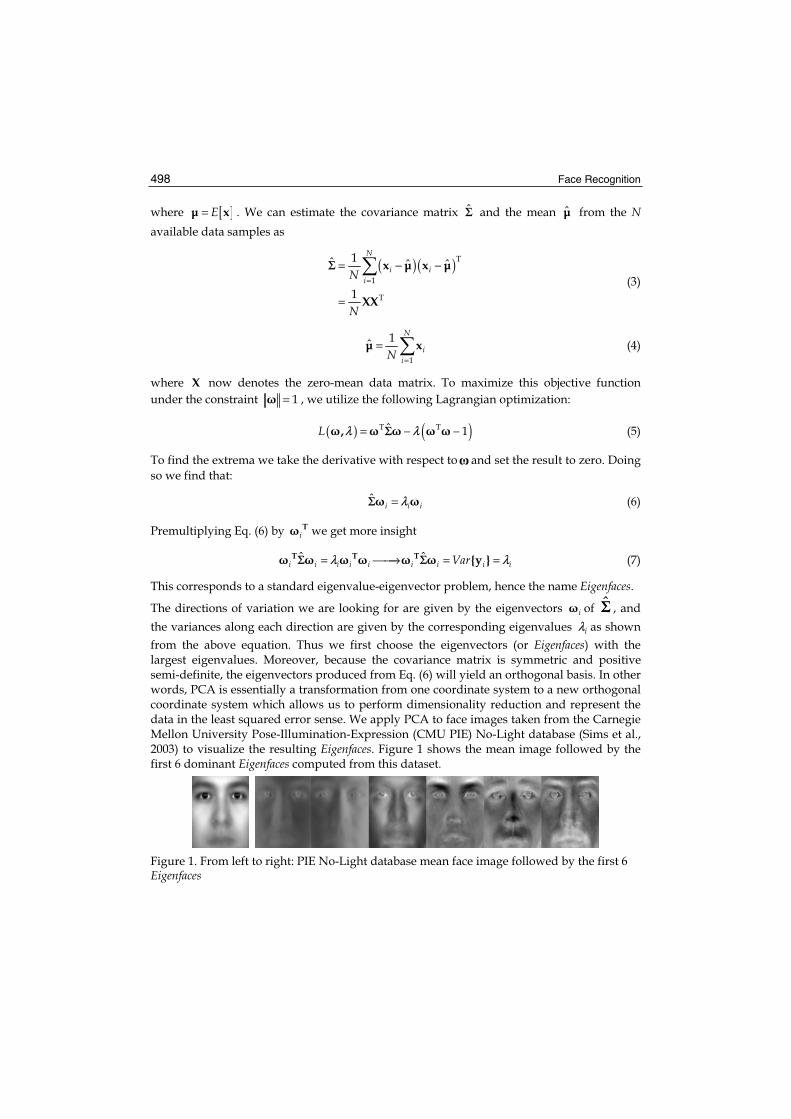
Face Recognition 498
where [ ]μ xE= . We can estimate the covariance matrix Σ and the mean μ from the Navailable data samples as
( )( )T
1
T
1
1
ˆ ˆ ˆx μ x μ
XX
N
i iiN
N
Σ=
= − −
=
(3)
1
1μ xN
iiN =
= (4)
where X now denotes the zero-mean data matrix. To maximize this objective function under the constraint = 1 , we utilize the following Lagrangian optimization:
( ) ( )= − −T T 1ˆ,L λ λΣ (5)
To find the extrema we take the derivative with respect to and set the result to zero. Doing so we find that:
=ˆi i iλΣ (6)
Premultiplying Eq. (6) by Ti we get more insight
= ⎯⎯→ = =T T Tˆ ˆ {y }i i i i i i i i iVarλ λΣ Σ (7)
This corresponds to a standard eigenvalue-eigenvector problem, hence the name Eigenfaces.
The directions of variation we are looking for are given by the eigenvectors i of ˆ , and the variances along each direction are given by the corresponding eigenvalues iλ as shown from the above equation. Thus we first choose the eigenvectors (or Eigenfaces) with the largest eigenvalues. Moreover, because the covariance matrix is symmetric and positive semi-definite, the eigenvectors produced from Eq. (6) will yield an orthogonal basis. In other words, PCA is essentially a transformation from one coordinate system to a new orthogonal coordinate system which allows us to perform dimensionality reduction and represent the data in the least squared error sense. We apply PCA to face images taken from the Carnegie Mellon University Pose-Illumination-Expression (CMU PIE) No-Light database (Sims et al., 2003) to visualize the resulting Eigenfaces. Figure 1 shows the mean image followed by the first 6 dominant Eigenfaces computed from this dataset.
Figure 1. From left to right: PIE No-Light database mean face image followed by the first 6 Eigenfaces
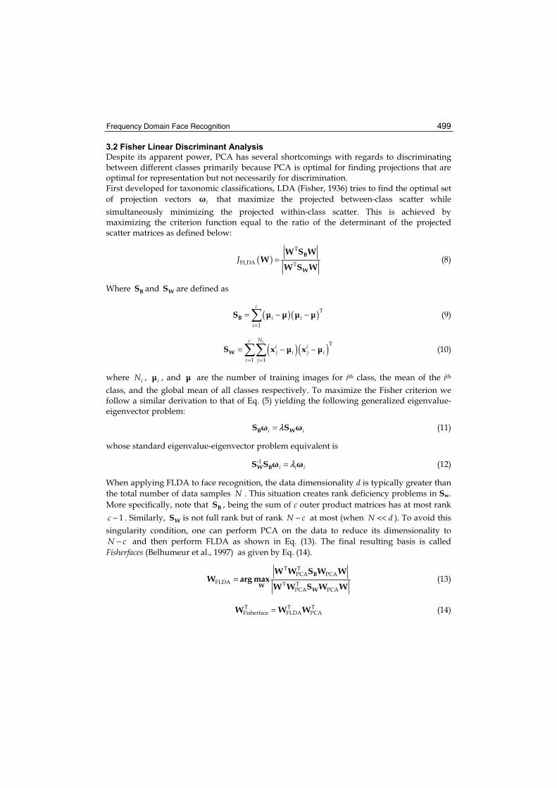
Frequency Domain Face Recognition 499
3.2 Fisher Linear Discriminant Analysis
Despite its apparent power, PCA has several shortcomings with regards to discriminating between different classes primarily because PCA is optimal for finding projections that are optimal for representation but not necessarily for discrimination. First developed for taxonomic classifications, LDA (Fisher, 1936) tries to find the optimal set of projection vectors i that maximize the projected between-class scatter while simultaneously minimizing the projected within-class scatter. This is achieved by maximizing the criterion function equal to the ratio of the determinant of the projected scatter matrices as defined below:
( )T
FLDA T
B
W
W S WW
W S WJ = (8)
Where BS and WS are defined as
( )( )T
1BS μ μ μ μ
c
i ii=
= − − (9)
( )( )T
1 1WS x μ x μ
iNci ij i j i
i j= =
= − − (10)
where iN , μi , and μ are the number of training images for ith class, the mean of the ith
class, and the global mean of all classes respectively. To maximize the Fisher criterion we follow a similar derivation to that of Eq. (5) yielding the following generalized eigenvalue-eigenvector problem:
B WS Si iλ= (11)
whose standard eigenvalue-eigenvector problem equivalent is
=-1W BS S i i iλ (12)
When applying FLDA to face recognition, the data dimensionality d is typically greater than the total number of data samples N . This situation creates rank deficiency problems in Sw.More specifically, note that BS , being the sum of c outer product matrices has at most rank
1c − . Similarly, WS is not full rank but of rank N c− at most (when <<N d ). To avoid this singularity condition, one can perform PCA on the data to reduce its dimensionality to N c− and then perform FLDA as shown in Eq. (13). The final resulting basis is called Fisherfaces (Belhumeur et al., 1997) as given by Eq. (14).
=T T
PCA PCAFLDA T T
PCA PCA
B
WW
W W S W WW arg max
W W S W W (13)
T T TFisherface FLDA PCAW W W= (14)

Face Recognition 500
3.3 Frequency Domain Extensions
It has been shown (Oppenheim et al., 1980) that phase information of an image holds the most salient information. In (Hayes et al., 1981), it is shown that one can reconstruct the original signal up to a scale factor given only phase information of the signal. This concept was exploited in face recognition to improve performance over standard algorithms (Savvides et al., 2004b). Figure 2 shows images of two different subjects; each image is split in Fourier domain between magnitude and phase. Figure 2 shows that when the first subject’s Fourier magnitude spectrum is coupled with the second subject’s Fourier phase spectrum, the resulting image in spatial domain shows significantly more similarity to the second subject compared to the first subject.
(a) (b) (c) (d) Figure 2. (a) Original image of first subject (b) Original image of second subject (c) Spatial domain image synthesized from combination of Fourier magnitude spectrum of first subject with Fourier phase spectrum of second subject (d) Spatial domain image synthesized from combination of Fourier magnitude spectrum of second subject with Fourier phase spectrum of first subject
However, performing PCA in the frequency domain alone does not constitute any breakthrough, this is because the eigenvectors obtained in the frequency domain are merely the Fourier transform of their spatial domain counterparts. We begin this derivation by defining the standard 2-D Discrete Fourier Transform (DFT) pair which is fundamental to the rest of our discussion. Given an 2-D discrete input signal [ ],x m n of size M × N we denote
its Fourier transform as [ ],X k l whose Fourier transform pair is defined as follows:
[ ] [ ]
[ ] [ ]
[ ] [ ]
1
2 2 ln1 1
0 0i2 i2 ln1 1
0 0
1
, ,
, ,
, ,
F
Fi km iM N
M N
m nkmM N
M N
k l
x m n X k l
X k l x m n e e
x m n X k l e eMN
−
− −− −
= =− −
= =
⎯⎯→←⎯⎯
=
=
(15)
where 1i = − , operator F is defined as the forward DFT, and the operator 1F− is the inverse DFT.
The estimated covariance matrix of the data in Fourier domain ˆf is given by Eq. (16)
where F is the d × d Fourier transform matrix containing the DFT basis vectors. The estimated covariance matrix of the data in Fourier domain is given as
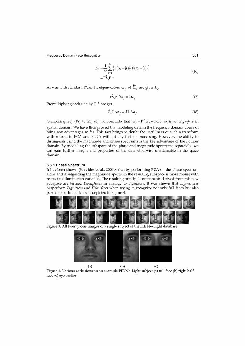
Frequency Domain Face Recognition 501
( ){ } ( ){ }1
1
1
ˆ ˆ ˆF x μ F x μ
ˆF F
N
f i ii
s
NΣ
Σ
+
=−
= − −
=
(16)
As was with standard PCA, the eigenvectors f of ˆf are given by
1ˆF Fs f fλΣ − = (17)
Premultiplying each side by 1F− we get
1 1ˆ F Fs f fλΣ − −= (18)
Comparing Eq. (18) to Eq. (6) we conclude that 1Fs f−= where s is an Eigenface in
spatial domain. We have thus proved that modeling data in the frequency domain does not bring any advantages so far. This fact brings to doubt the usefulness of such a transform with respect to PCA and FLDA without any further processing. However, the ability to distinguish using the magnitude and phase spectrums is the key advantage of the Fourier domain. By modelling the subspace of the phase and magnitude spectrums separately, we can gain further insight and properties of the data otherwise unattainable in the space domain.
3.3.1 Phase Spectrum
It has been shown (Savvides et al., 2004b) that by performing PCA on the phase spectrum alone and disregarding the magnitude spectrum the resulting subspace is more robust with respect to illumination variation. The resulting principal components derived from this new subspace are termed Eigenphases in analogy to Eigenfaces. It was shown that Eigenphasesoutperform Eigenfaces and Fisherfaces when trying to recognize not only full faces but also partial or occluded faces as depicted in Figure 4.
Figure 3. All twenty-one images of a single subject of the PIE No-Light database
(a) (b) (c) Figure 4. Various occlusions on an example PIE No-Light subject (a) full face (b) right half-face (c) eye section

Face Recognition 502
(a) (b) Figure 5. Rank-1 identification rates obtained by Eigenphases, Eigenfaces, and Fisherfaces for two different experiments each using different types of partial faces. (a) right half face (b) eye-section face
In this work, comparisons between Rank-1 identification rates obtained from Eigenphases,Eigenfaces, and Fisherfaces are made when using whole and partial faces. Training is done on multiple subsets of the PIE database while testing is performed over the whole database. Fifteen different training subsets each representing different types of illumination with the first seven having the most or harshest illumination variation with the remaining eight containing near frontal lighting which are considered the most neutral lighting conditions. Figure 5 depicts the recognition rates obtained with the three different methods using half-faces and eye-sections. These results show that not only do Eigenphases outperform Eigenfaces and Fisherfaces for all experiments by a wide margin, but they also demonstrate minimal performance degradation for half-faces and eye-section faces. This added occlusion robustness is a very attractive property in real-world applications where missing data and poor data quality are common problems.
3.3.2 Magnitude Spectrum
In contrast, if PCA is performed on the magnitude spectrum only, it has been shown (Bhagavatula & Savvides, 2005a) that the resulting subspace holds many advantages over spatial subspaces. Using the Olivetti Research Laboratory (ORL) database, which is noted for significant pose variation, it was shown that the Fourier Magnitude Principal Component Analysis (FM-PCA) subspace yielded higher recognition rates across a range of experiments. These experiments included varying the number of training images whose comparison to spatial domain PCA or Eigenfaces is illustrated in Figure 6 (a). It was also shown that FM-PCA is more robust to noise as demonstrated in Figure 6 (b). This was verified by corrupting the testing images with varying levels of Additive White Gaussian Noise (AWGN). In similar fashion, it was demonstrated that Fourier Magnititude Fisher Linear Discriminant Analysis (FM-FLDA) clusters data better than traditional Fisherfaces with decreased within-class scatter and increased between-class scatter. FM-FLDA yields higher recognition rates for varying image sizes and resolutions in comparison to spatial FLDA or Fisherfaces as tabulated in Table 1.
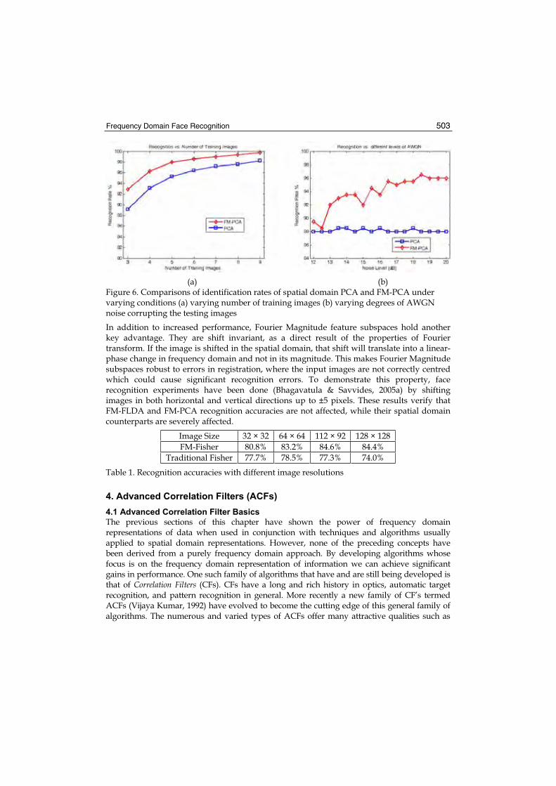
Frequency Domain Face Recognition 503
(a) (b) Figure 6. Comparisons of identification rates of spatial domain PCA and FM-PCA under varying conditions (a) varying number of training images (b) varying degrees of AWGN noise corrupting the testing images
In addition to increased performance, Fourier Magnitude feature subspaces hold another key advantage. They are shift invariant, as a direct result of the properties of Fourier transform. If the image is shifted in the spatial domain, that shift will translate into a linear-phase change in frequency domain and not in its magnitude. This makes Fourier Magnitude subspaces robust to errors in registration, where the input images are not correctly centred which could cause significant recognition errors. To demonstrate this property, face recognition experiments have been done (Bhagavatula & Savvides, 2005a) by shifting images in both horizontal and vertical directions up to ±5 pixels. These results verify that FM-FLDA and FM-PCA recognition accuracies are not affected, while their spatial domain counterparts are severely affected.
Image Size 32 × 32 64 × 64 112 × 92 128 × 128FM-Fisher 80.8% 83.2% 84.6% 84.4%
Traditional Fisher 77.7% 78.5% 77.3% 74.0%
Table 1. Recognition accuracies with different image resolutions
4. Advanced Correlation Filters (ACFs)
4.1 Advanced Correlation Filter Basics
The previous sections of this chapter have shown the power of frequency domain representations of data when used in conjunction with techniques and algorithms usually applied to spatial domain representations. However, none of the preceding concepts have been derived from a purely frequency domain approach. By developing algorithms whose focus is on the frequency domain representation of information we can achieve significant gains in performance. One such family of algorithms that have and are still being developed is that of Correlation Filters (CFs). CFs have a long and rich history in optics, automatic target recognition, and pattern recognition in general. More recently a new family of CF’s termed ACFs (Vijaya Kumar, 1992) have evolved to become the cutting edge of this general family of algorithms. The numerous and varied types of ACFs offer many attractive qualities such as

Face Recognition 504
shift invariance, normalized outputs, and noise tolerance. Their derivations require some knowledge in such fields as linear algebra, signal processing, and detection and estimation theory. We will assume that readers will have sufficient background in these fields and only elucidate on background information when is necessary. We will also now limit our discussion to two-dimensional applications which include facial recognition using grayscale imagery. To begin the discussion we define a few fundamental terms and conventions that will be used repeatedly for the span of this section. The application of a CF or ACF to an input image will yield a correlation plane. The centre or origin of correlation plane will be considered to be the spatial position (0, 0). Analysis of the correlation plane to some metric of performance or confidence will usually involve calculation and identification of the largest value or peak in the correlation plane.. The simplest CF is the Matched Filter (MF), commonly used in applications such as communication channels and radar receivers where the goal is detecting a known signal in additive noise. The concept of noise is a very important aspect of pattern recognition problems. To characterize noise we define the quantitative measure of Power Spectral Density (PSD). Using this characterization of noise the MF is developed with the goal of maximizing the Signal-to-Noise-Ratio (SNR). Fundamentally this is equivalent to describing a filter whose application to an input signal will minimize the effect of specific type of noise while maximizing the output value when presented with the desired input signal. We will not develop the MF, however multiple other sources provide detailed derivations for varying applications and should be consulted for more information. We will use this fundamental concept of maximizing the response of the desired signal or pattern and minimizing the effects of noise as a guideline in our derivation of ACFs. One of the fundamental differences between typical CFs and ACFs is the ability to synthesize ACFs from multiple instances of training data or in the case of face recognition, multiple facial images and by doing so, to be able to recognize all instances which are present in the training data. The desire or hope here is that the training data sufficiently represents or captures the potential distortion or variation that might be presented to the recognition system. With respect to face recognition systems this is an extremely desirable quality because the human face is subject to numerous variations both intrinsic and extrinsic. By allowing such variations to be at least partially represented through the use of representative training data we can increase both performance and robustness of face recognition systems.
4.2 Correlation Basics
Before we can derive any ACF we must first lay the framework of correlation with respect to 2D imagery. The standard definition of discrete 2-D correlation between an input 2-D signal
( )x m, n and a 2-D filter ( )h m, n resulting in 2D correlation output plane ( )y m, n is as follows:
( ) ( ) ( )
( ) ( )
( ) ( )nm, lkhk, lx
k, lhlk, nmx
m, nhm, nxm, ny
k l
k l
−−=
++=
⊗=
∞
∞=
∞
∞=
∞
∞=
∞
∞=
- -
- -
(19)

Frequency Domain Face Recognition 505
We will only consider the case of discrete correlation as this is the case of interest in face recognition systems although the analog domain provides some desirable qualities and generalizations. However, for our purposes the desired properties of both correlation and the Fourier transform are present in the discrete domain. Using the Fourier transform and its properties as discussed previously we can express Eq. (19) in the frequency domain as
( ) ( ) ( )( ) ( ){ }1 *
y m, n x m, n h m, n
F X k, l H k, l−
= ⊗
= ⋅ (20)
where ( )X k, l and ( )H k, l are the 2-D Fourier transforms of ( )x m, n and ( )h m, n respectively.
The symbols 1F− , ⋅ , and * represent the inverse Fourier transform, the element by element (point to point) multiplication of the two 2-D signals, and the element by element conjugation respectively. Correlation in the frequency domain is vastly preferred to correlation in the spatial domain with regards to the number computational floating point operations required.
4.3 Synthetic Discriminant Functions
One of the first ACFs to incorporate such a composite design is the Synthetic Discriminant Function filter (Hester & Casasent, 1980). The design of the Synthetic Discriminant Function(SDF) filter is that the filter is created such that it yields a correlation plane whose output at the origin yields a pre-specified value. By introducing such a constraint on the output we not only allow for normalized comparisons but also a degree of discrimination into our filters. This framework refers to the ability to use a single filter to recognize different patterns or classes with sufficient discrimination as opposed to using a single filter for each class or image sample (as with the case of MFs). For example, in a two class problem we would like to design a filter yields an output value of 1 for class 1 while yielding an output value of 0 for class 2. We can achieve this by constraining the correlation plane outputs (at the origin) to be 1 for all training data from class 1 and 0 for all training data from class 2. Our derivation of the SDF filter begins with an outline of the basic variables and problem definition. Let us assume that we have N facial training images ( )ix m, n of size d1 × d2. Define
ui to be the output value of the correlation plane ( )iy m, n ; that is the result of applying the
filter ( )h m, n to the training image ( )ix m, n . Please note that the output value of the correlation plane is considered to be the value of the correlation plane at the origin or equivalently ( )0, 0iy . Thus we can define the following equation,
( ) ( ) ( ) Nim, nhm, nxyud
m
d
niii ≤≤==
= =
100,1 2
1 1
, (21)
The above equation explicitly demonstrates the correlation operation and the constraint on the correlation plane output value at the origin. However, for convenience we can rewrite the above equation into a more compact vector format. Suppose we take a training image ( )ix m, n (of dimensions d1 x d2) and place its entries (vectorize) from left to right and
top to bottom into a column vector xi of length d = d1 x d2 and similarly for ( )h m, n intocolumn vector h whose length is also d. We can now express Eq. (21) in the following form,
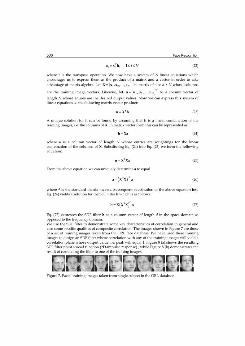
Face Recognition 506
Niu ii ≤≤= 1T ,hx (22)
where T is the transpose operation. We now have a system of N linear equations which encourages us to express them as the product of a matrix and a vector in order to take advantage of matrix algebra. Let [ ]1 2X x ,x , , xN= be matrix of size d × N whose columns
are the training image vectors. Likewise, let [ ]T1 2u u ,u , ,uN= be a column vector of
length N whose entries are the desired output values. Now we can express this system of linear equations as the following matrix vector product:
hXu T= (23)
A unique solution for h can be found by assuming that h is a linear combination of the training images, i.e. the columns of X. In matrix vector form this can be represented as
Xah = (24)
where a is a column vector of length N whose entries are weightings for the linear combination of the columns of X. Substituting Eq. (24) into Eq. (23) we form the following equation:
Tu X Xa= (25)
From the above equation we can uniquely determine a to equal
( ) 1Ta X X u-
= (26)
where -1 is the standard matrix inverse. Subsequent substitution of the above equation into Eq. (24) yields a solution for the SDF filter h which is as follows:
( ) 1Th X X X u-
= (27)
Eq. (27) expresses the SDF filter h as a column vector of length d in the space domain as opposed to the frequency domain. We use the SDF filter to demonstrate some key characteristics of correlation in general and also some specific qualities of composite correlation. The images shown in Figure 7 are those of a set of training images taken from the ORL face database. We have used these training images to design an SDF filter whose correlation with any of the training images will yield a correlation plane whose output value, i.e. peak will equal 1. Figure 8 (a) shows the resulting SDF filter point spread function (2D-impulse response) , while Figure 8 (b) demonstrates the result of correlating the filter to one of the training images.
Figure 7. Facial training images taken from single subject in the ORL database
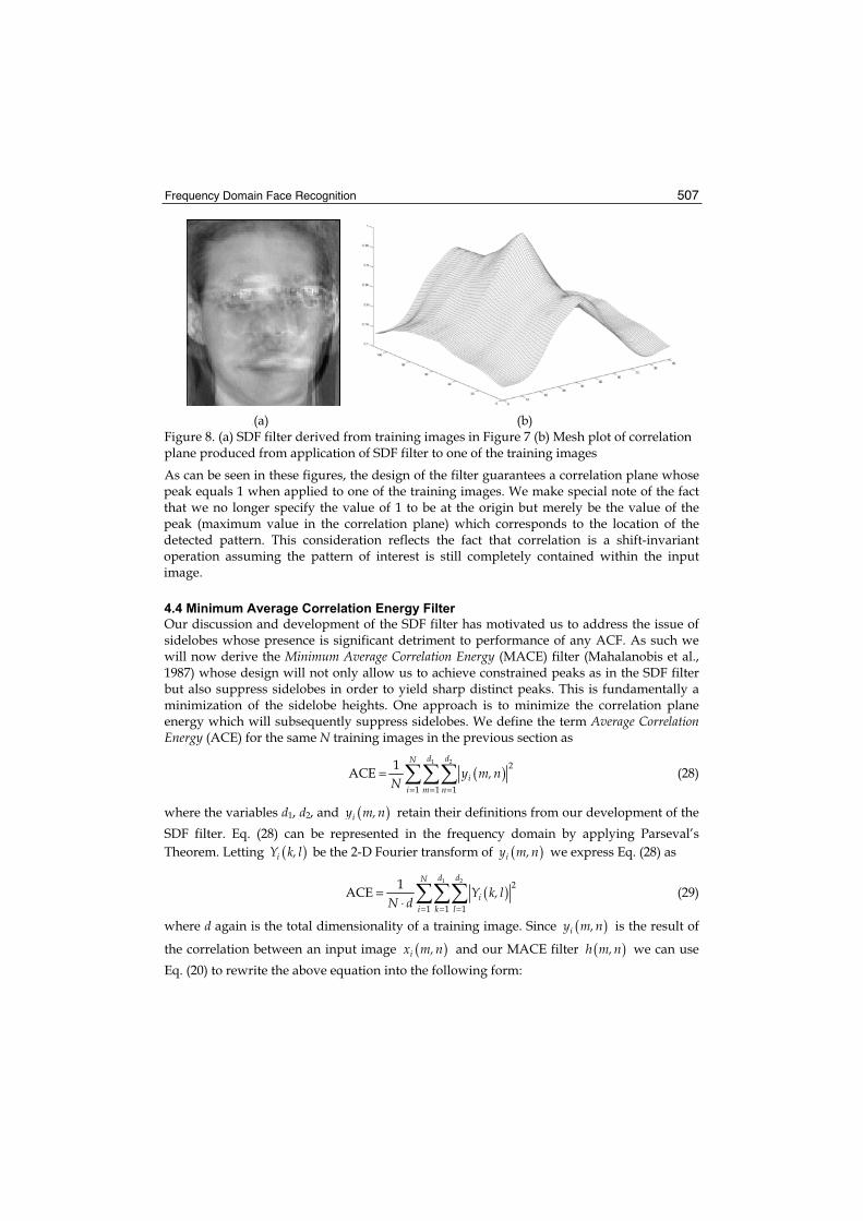
Frequency Domain Face Recognition 507
.(a) (b) Figure 8. (a) SDF filter derived from training images in Figure 7 (b) Mesh plot of correlation plane produced from application of SDF filter to one of the training images
As can be seen in these figures, the design of the filter guarantees a correlation plane whose peak equals 1 when applied to one of the training images. We make special note of the fact that we no longer specify the value of 1 to be at the origin but merely be the value of the peak (maximum value in the correlation plane) which corresponds to the location of the detected pattern. This consideration reflects the fact that correlation is a shift-invariant operation assuming the pattern of interest is still completely contained within the input image.
4.4 Minimum Average Correlation Energy Filter
Our discussion and development of the SDF filter has motivated us to address the issue of sidelobes whose presence is significant detriment to performance of any ACF. As such we will now derive the Minimum Average Correlation Energy (MACE) filter (Mahalanobis et al., 1987) whose design will not only allow us to achieve constrained peaks as in the SDF filter but also suppress sidelobes in order to yield sharp distinct peaks. This is fundamentally a minimization of the sidelobe heights. One approach is to minimize the correlation plane energy which will subsequently suppress sidelobes. We define the term Average Correlation Energy (ACE) for the same N training images in the previous section as
( )1 2 2
1 1 1
1ACEd dN
ii m n
y m, nN = = =
= (28)
where the variables d1, d2, and ( )iy m, n retain their definitions from our development of the SDF filter. Eq. (28) can be represented in the frequency domain by applying Parseval’s Theorem. Letting ( )iY k, l be the 2-D Fourier transform of ( )iy m, n we express Eq. (28) as
( )1 2 2
1 1 1
1ACEd dN
ii k l
Y k, lN d = = =
=⋅
(29)
where d again is the total dimensionality of a training image. Since ( )iy m, n is the result of
the correlation between an input image ( )ix m, n and our MACE filter ( )h m, n we can use Eq. (20) to rewrite the above equation into the following form:

Face Recognition 508
( ) ( )1 2 2 2
1 1 1
1ACEd dN
ii k l
X k, l H k, lN d = = =
=⋅
(30)
It should be noted that it is at this point in the derivation where the role of the frequency domain representations of both the data and the filter are fundamental to the filter design. Later ACF designs will also utilize the quantitative measure of ACE along with other such measures. For now let us to proceed to again represent Eq. (30) in matrix vector form. Let hbe a column vector of length d whose elements are taken from ( )H k, l and Xi be a diagonal
matrix of size d × d whose non-zero elements are taken from ( )iX k, l . Using these frequency domain terms we can express Eq. (30) as
( )( )1
1ACE h X X hN
i iiN d
+ ∗
=
=⋅
(31)
where the symbol + indicates the conjugate transpose. We can compress this expression further by defining a new diagonal matrix D of size d × d as follows:
1
1D X XN
i iiN d
∗
=
=⋅
(32)
This allows us to express the quantity of ACE in very concise manner as
Dhh+=ACE (33)
Our goal in the design of the MACE filter is the minimization of the ACE of the training images while still satisfying the peak constraints we have specified. To accomplish this we must express these constraints in the frequency domain as well. Due to the fact that inner products in the frequency domain (at the origin only) are equivalent to inner products in the spatial domain, we can rewrite the peak constraints expressed in Eq. (23) as
uhX ⋅=+ d (34)
where X is a matrix of size d × N whose columns are the vector representations of the FTs of the training images. Thus, the filter h which minimizes Eq. (33) while satisfying the constraints expressed in Eq. (34) is our MACE filter. This constrained optimization can be solved using Lagrange multipliers, which can be found in the original paper (Mahalanobis et al., 1987), which yield the final solution to the frequency domain filter h:
( ) 11 1h D X X D X u−− + −= (35)
The notation and form of the solution allows for simple and efficient calculation of the filter in column vector form from which a simple reshaping operation can be done to recover the 2-D frequency domain filter of size d1 × d2. Correlation of the filter with an input image now requires one less Fourier transform as the filter is already represented and stored in the

Frequency Domain Face Recognition 509
frequency domain. Using the same training images from our derivation of the SDF filter we can create a MACE filter whose output correlation planes will not contain the problematic sidelobes. Visualizing the point spread function of the MACE filter itself does not reveal much insight without more significant analysis, but the goals of ACE minimization and constrained peaks are achieved as shown in Figure 9. Not only is the peak equal to 1 as specified, but the sidelobes are drastically suppressed when compared to those in the SDF filter’s correlation plane in Figure 8 (b). Noise tolerance can be built in as discussed in the next section.
Figure 9. Mesh plot of correlation plane produced from application of MACE filter to one of the training images
4.5 Minimum Variance Synthetic Discriminant Function
Through our derivations of the SDF and MACE filters we have shown that in order to achieve high discriminative ability in our filters we must be able to control the correlation plane through constraints and sidelobe energy minimizations. However, in any practical application we must always take into consideration the factor of noise introduced from varying sources. Whether it is sensor noise or noise caused by background clutter, the presence of noise can have significant impact on any face recognition system. As such we would like to introduce into our ACF designs some degree of noise tolerance. Let us formalize the problem with the following equation:
( )T T Tx v h x h v hu
+ = += + δ
(36)
where x is an image vector and v is the additive noise vector whose responses to the filter vector h are u and δ respectively. The variations in the outputs of our filter are due to δand therefore δ is the quantity we wish to suppress. For the rest of the derivation we will assume that our noise processes are stationary. We will also assume that our noise is zero mean without any loss of generality. To suppress the effect of variation in our filter outputs due to noise we aim to minimize the variance of the output noise term δ . Denote this variance as the Output Noise Variance (ONV) whose definition is

Face Recognition 510
{ }( ){ }{ }
{ }
2
2T
T T
T T
T
ONV
v h
h vv h
h vv h
h Ch
E
E
E
E
=
=
=
=
=
δ
(37)
where C is the covariance matrix of the input noise. We take note of the independence of ONV from the image vector x which implies that its definition is identical for all images of interest. Let us now consider the training images we used in developing the SDF filter whose derivation focused on achieving certain constraints placed on output peak values. We would now like to not only achieve those same constraints expressed in Eq. (23) but also minimize the ONV amongst our training images. This formulation lends itself to the use of Lagrange minimization almost identical to that used in the formulation of the MACE filter to yield the following filter solution:
( ) 11 1h C X X C X u−− + −= (38)
The above filter is referred to as the Minimum Variance Synthetic Discriminant Function(MVSDF) filter (Vijaya Kumar, 1986). While the MVSDF filter does achieve minimum ONV amongst its training images, it does not suppress ACE and as such suffers from unsuppressed sidelobes. In later ACF designs we will show how to achieve an optimal tradeoff between ONV and ACE minimization in order to provide varying degrees of simultaneous noise tolerance and sidelobe suppression.
4.6 Maximum Average Correlation Height Filter
All of the ACFs we have described to this point have been designed with some constraint or optimization in mind that is meant to introduce distortion tolerance into our filters. However, this is but one way and perhaps not the best way to create distortion tolerance. There is no formalized relationship between the constraints we have described so far and the degree of distortion tolerance incorporated into the filter. A more intuitive approach is to remove these constraints to allow for more solutions. In essence this is akin to generalizing the solution space which will hopefully contain solutions to non-training images. This would result in a greater degree of distortion tolerance when compared to ACFs derived using hard constraints. To address the issue of distortion tolerance it is necessary to first quantize the amount of distortion present in a set of filtered images. To this end we define the Average Similarity Measure (ASM) over a set of N filtered images ( )iy m, n as
( ) ( )( )N
2
1
1ASM ii m n
y m, n y m, nN =
= − (39)

Frequency Domain Face Recognition 511
where we define ( )y m, n as the average image whose exact definition is
( ) ( )1
1 N
jj
y m, n y m, nN =
= (40)
ASM is a measure of the average variation amongst a set of correlation surfaces. As was with previous ACFs we recognize the fact that the above spatial domain equation is equivalently expressed in the frequency domain by applying Parseval’s theorem. Let
( )iY k, l be the 2D-Fourier transform of ( )iy m, n and ( )Y k, l be the 2D-Fourier transform
of ( )y m, n . Also, because we are primarily concerned with the frequency domain let us
express ( )iY k, l and ( )Y k, l as the column vectors yi and y respectively. Eq. (39) is equivalently represented in the frequency domain as
( ) ( )1 2N 2
1 1 1N
2
1
1ASM
1 y y
d d
ii k l
ii
Y k, l Y k, lN d
N d
= = =
=
= −⋅
= −⋅
(41)
We must now introduce the filter itself into this metric to allow for optimization with respect to the filter coefficients. Let us consider the ASM over a set of correlation surfaces which are the result of filtering a set N training images ( )ix m, n with the filter ( )h m, n . As such let us express the Fourier transforms of the ith training image and the filter as
( )iX k, l and ( )H k, l respectively. Also, define ( )X k, l , the average Fourier transform of the N training images, as
( ) ( )1
N
ii
X k, l X k, l=
= (42)
We proceed by representing ( )iX k, l , ( )X k, l , ( )H k, l as column vectors xi , x , and h
respectively. Let us now define the diagonal matrices Xi and X whose non-zero elements are taken respectively from xi and x . Using these matrices we can express yi and y as
y X hi i∗= (43)
y X h∗= (44)
Substituting the above equations in to Eq. (41) we have the following equivalent expression:
( )( )
N 2
1N
1
1ASM
1
X h X h
h X X X X h
h Sh
ii
i ii
N d
N d
∗ ∗
=
∗+
=+
= −⋅
= − −⋅
=
(45)

Face Recognition 512
where the diagonal matrix S is defined as
( )( )N
1
1S X X X Xi iiN d
∗
=
= − −⋅
(46)
We have now expressed the distortion metric of ASM as a function of the filter and the training images. However, while minimizing distortion we also wish to maximize the filter’s response to authentic patterns/faces. Unlike the MACE filter we have no constraint on the peak value and thus our desire is to maximize the correlation peak value over the entire set of training images i.e., maximize the average peak value. We denote this quantity by the measure of Average Correlation Height (ACH) whose definition is
( )
( )
( ) ( )
1 2
1 2
1
1 1 1
1 1 1
1ACH 0, 0
1 ,
1 , ,
N
ii
d dN
ii k l
d dN
ii k l
yN
Y k lN d
X k l H k lN d
=
= = =
∗
= = =
=
=⋅
=⋅
(47)
whose matrix vector formulation utilizing previously defined vectors xi , x , and h is
1
1ACH x h
x h
N
iiN
+
=+
=
=
(48)
While our immediate goal is to suppress ASM while maximizing ACH it is of course also desirable to suppress ONV as defined earlier. This simultaneous minimization maximization problem lends itself to a Rayleigh quotient representation as follows:
( )
( )
2
2
2
ACHASM+ONV
h
m h
h Sh h Ch
m h
h S C h
J
+
+ +
+
+
=
=+
=+
(49)
The filter h that maximizes this ratio is the dominant eigenvector of ( )-1S C mm++ which is
( )-1h S C m= +α (50)
where α is a normalizing coefficient. The above filter solution is termed the Maximum Average Correlation Height (MACH) filter (Mahalanobis et al., 1994). The MACH filter is often used in ATR applications where its tolerance for noise and distortion addresses the issue of

Frequency Domain Face Recognition 513
sensor noise and background clutter while maintaining the ability to resolve sharp and distinct correlation peaks necessary for accurate target detection and recognition. These same issues are paralleled in many face recognition applications and as such the same characteristics of the MACH filter are desired.
4.7 Optimal Tradeoff Filters
We have thus far developed ACFs whose derivation incorporate different desirable qualities such as the MACE filter’s ability to resolve sharp correlation peaks, or the MVSDF filter’s tolerance for noise. However, while these filter solutions provide these attractive properties they inherently create deficiencies in other aspects. For example, the MACE filter while being able to resolve sharp peaks, has little tolerance for noise while the MVSDF filter’s tolerance for noise is offset by its relative inability to generate sharp correlation peaks. The fundamental issue concerning these particular ACFs is their singular focus on optimality with respect to one aspect of distortion. Depending on the application, a more preferred approach might be to design a filter whose optimality in these varying aspects is variable. In other words, we desire a filter which maintains a tradeoff between peak sharpness and noise tolerance. Termed Optimal Tradeoff (OT) filters, we will not go through the complete derivation in the interest of conciseness and its similarity to previous derivations. The OT filter counterpart for the MACE and MVSDF filter is referred to as the Optimal Tradeoff Synthetic Discriminant Function (OTSDF) filter (Vijaya Kumar, 1994). It is obtained by minimizing a weighted sum of ACE and ONV which are the metrics for the MACE and MVSDF filters respectively. The resulting filter solution is
( ) ( )11 1h D C X X D C X u
−− −+= + +α β α β (51)
where α and β are non-negative constants that can be varied to achieve a desired amount of performance with respect to noise and peak sharpness while all other variables retain their definitions from previous sections. In order better constrain the relationship between the tradeoff between noise tolerance and peak sharpness we constrain the relationship between α and β with the following:
2 2 1+ =α β (52)
This constraint is a result of the quadratic nature of the filter solution (Vijaya Kumar, 1994) Allowing us to rewrite Eq. (51) as function of α alone in the following manner:
( ) ( )11 1
1 1h D C X X D C X u−− −
+= + − + −2 2α α α α (53)
Since α is non-negative, we can vary the amount of noise tolerance and peak sharpness in the filter by varying α between 0 and 1. If we were to set α to 0, then Eq. (53) reduces to the MVSDF filter solution in Eq. (38) while and α of 1 yields the MACE filter solution of Eq. (35). By choosing values of α in this range we are essentially creating a filter which is a weighted combination of the MACE and MVSDF filters. Typically α is set close to 1 in order to maintain sharp peaks while incorporating a small degree of noise tolerance. Most experiments concerning the effect of α on filter performance have supported this notion.

Face Recognition 514
(a) (b)
(c) (d) Figure 10. Mesh plots of correlation planes produced from application of OTSDF filter expecting AWGN of SNR 20 dB to a training image with varying values of α (a) 0=α (b)
0.33=α (c) 0.67=α (d) 1.00=α
However, one must take into account the type and degree of noise the filter is being designed to accommodate for. In many applications Additive White Gaussian Noise (AWGN) is the standard form of noise for which depending on its magnitude or equivalently its SNR can be negligible. However, when the magnitude of the noise is non-negligible we can observe the effect of α paremeter upon the filter design and any subsequent correlation planes. Figure 10 demonstrates this aspect of the OTSDF filter by presenting the correlations of one of the training images with four OTSDF filters each designed with different values of α and expecting AWGN of SNR 20 dB. The most noticeable change between the correlation planes is the relative strength of the sidelobes throughout the correlation plane. Since the MACH filter is often thought of as the unconstrained version of the MACE filter, we call the MACH filter’s OT filter the Unconstrained Optimal Tradeoff Synthetic Discriminant Function (UOTSDF) filter (Vijaya Kumar, 1994). The solution to the UOTSDF filter is

Frequency Domain Face Recognition 515
( ) 1h D C S m−= + +α β γ (54)
where α , β , and γ are tradeoff parameters for ACE, ONV, and ASM respectively while all other variables retain their previous definitions. Though there exists a quadratic relationship between these parameters we often choose to fix at least one parameter while optimizing the others with respect to performance.
4.8 Performance Measures
When considering the use of correlation in pattern recognition and in particular face recognition applications it becomes necessary to define a metric by which to quantify the “goodness” or “correctness” of a correlation. A simple and sometimes effective way to quantize a match is to take the largest value in a correlation plane and threshold it to yield a match or no-match decision. This approach works well when there is relatively small variation in the data such that the variance in the value of the correlation peak is small. This assumption is of course is an idealization and, with particular focus on face recognition, a poor one. The value of the correlation peak will vary in the presence of intensity changes and noise in non-negligible amounts and as such a strict threshold cannot be expected to be a reliable performance measure. When considering such ACFs as the MACE and OTSDF filters a more appropriate measure is that of peak sharpness since these filters are designed to suppress the sidelobes adjacent to peaks. This relationship can be quantized by the Peak-to-Sidelobe Ratio (PSR) which for a particular peak is defined as
( ) area
area
peak valuePSR
−=
μσ
(55)
where areaμ and areaσ are the mean and standard deviation respectively of some small area or neighborhood around but not including the peak. Similarly the MACH and UOTSDF filters are designed to maximize the value of the peak relative to the rest of correlation plane also. Thus a similar but alternate performance measure would be one that measured the magnitude of difference between the peak and the rest of the correlation plane. Using the metric of Peak-to-Correlation Energy (PCE) we can quantify this difference as
( ) plane
plane
peak valuePCE
−=
μσ
(56)
where planeμ and planeσ are the mean and standard deviation respectively of the entire correlation plane excluding the peak. Both PSR and PCE can be used with any ACF but the optimal measure often depends on the application. In most situations where the resolution or size of the target is relatively constant as is the case with many face recognition applications, PSR is a sufficient measure. On the other hand, algorithms that use multi-resolution techniques might benefit more from PCE. Regardless, both measures still require a threshold to determine a match or no-match decision although in contrast with a strict threshold on the peak value alone, a threshold on PSR or PCE values is far more normalized and predictable.

Face Recognition 516
5. Face Recognition Using Advanced Correlation Filters
5.1 Face to Sketch Correlation
One of the primary issues in many face recognition systems is that of illumination variation. An innumerable number of changing factors determine the exact nature of the illumination a face may be subject to at any given time. As such, the span of illumination variation is vast and often of non-negligible magnitude. In order for a face recognition system to objectively make the claim that it is capable of unrestricted field deployment it must be able to compensate for any type of illumination variation. One approach to this issue is to re-train the recognition system each time it is presented with a new environment or situation where the illumination has varied from previously known conditions. This can be costly both in terms of time and money and most of the time, this is not feasible or possible to capture all possible lighting conditions (especially when outdoors) so as a result this is not done in practice. Another approach is to incorporate some sort of illumination-preprocessing algorithm in order to compensate for varying illuminations. This method is much preferred to the former due to its hopefully broader and more effective application. Nonetheless, deriving such a preprocessing stage is in itself challenging given the degree of illumination compensation one is attempting to achieve. One of the more novel approaches to this problem involves using eigenanalysis and ACFs to reconstruct and recognize images respectively using a different representation of the face (Li et al., 2006). The relative uniqueness of this approach can be traced to the fact that it utilizes both traditional facial images coupled with corresponding facial sketches thsat are similar to those found in law enforcement. Consider the field of law enforcement applications where one of the most commonly used tools is that of a police sketch which is used to to help identify suspect criminals. Although visual surveillance equipment is present in many everyday environments, they are often of low quality and are not optimal for enrolling police sketches. To this end, the role of the witness becomes exceptionally important as a source of more reliable evidence. The police sketch allows the witness’ recollection of a suspect to manifest itself as a piece of visual evidence. Nonetheless the usefulness of the previously mentioned surveillance equipment should not be discounted. In many high security locations, continuous video surveillance is present and provides us with some record of people who have passed through those monitored locations. However, due to factors such as time of day and physical setup of the surveillance equipment, the exact lighting conditions which illuminate the faces of the passing people can vary. The issue now becomes one of recognizing the suspect in the surveillance data using the witness’ police sketch as the template. This kind of question can be categorized as robust face recognition for illumination variation. However this application is different from the normal face recognition scenario; where the enrollment gallery image is a real face image, as in this case the enrollment gallery image for finding the suspect from surveillance video is a police sketch of the suspect’s face. Of course there are strong similarities and high correlations between the real face images and the corresponding police sketch image. If one can capture the correlation between these two representations of same person, and describe those correlations in a useful mathematical form, then it will be very useful for finding a solution to this problem. In literature, there are two main types of approaches proposed for this kind of face-sketch dual space modeling problem. Both methodologies utilize eigenanalysis to form a basis for representing the face-sketch dual space, similar to how eigenanalysis is used in PCA and Eigenface applications. However, these two methodologies differ in the way of how they

Frequency Domain Face Recognition 517
form the eigen-subspace and how they capture the correlation between the two subspaces (i.e., face and sketch subspace). The first approach tries to construct the PCA subspace for both the face and sketch images separately, by transforming all the training data (which are real face images) into corresponding sketch images, and then perform classification in sketch space (Tang et al., 2002), this approach may face issues in practice as images with illumination variation will generate sketches with artifacts. The second approach to this problem tries to reconstruct the original face image from the given sketch image using a hybrid-eigenspace representation, and then perform classification using ACFs (Li et al., 2006). In the next few paragraphs, we will look at more details of this algorithm. The key idea us that a face recognition system, which takes surveillance footage, typically is subject to variable and unknown illumination artifacts and will not be able to synthesize good sketch images (corresponding to the illumination distorted face image) on the fly due illumination variation artifacts. These artifacts will be enhanced and significantly affect the resulting automatically generated sketch image. which will in turn ultimately affect recognition performance. In our proposed approach we reconstruct what the person ‘looks-like’ from the sketch image and then use this reconstructed image as the gallery enrollment image in the face recognition system which can recognize the person under the presence of illumination variations (as demonstrated with example experiments on the PIE database). We can use three stages to describe this algorithm: the training stage, the synthesis stage, and the recognition stage. Assume the training data has N face images and their corresponding N sketch images. We denote the ith face image as fi , and the ith sketch image as si where = …1 2 , , ,i N . By appending each face image with its corresponding sketch counterpart, we can form a new subspace, which is called “hybrid-subspace” in (Li et al., 2006). Then we can describe all of the training data in the following matrix form:
1
1
fh
s
D f fD =D s s
m
m
…=…
(57)
where each fi and si are column vectors, and fD consists of the face data matrix, and sDas the corresponding sketch data matrix. Our next step is to derive an orthonormal basis that represents our combined face data. Therefore, standard PCA is performed on the hybrid data matrix hD . We first remove the mean of the data by computing μf and μs:
=
=1
1fμ f
N
iiN
(58)
=
=1
1sμ s
N
iiN
(59)
…=…
1
1
f f m f
s f m f
X f - μ f - μX =X s - μ s - μ
(60)
Then the covariance matrix is defined as: 1 T= XXN
(61)
Face Recognition 518
Once we have , we perform eigenanalysis to derive its eigenvectors and eigenvalues:
h h h= (62)
where 1h m= … such that i is the ith eigenvector of , and ( )1h mdiagΛ = …
such that i represents the ith eigenvalue. Because every single column in hD contains a face image and its corresponding sketch images, each i can be interpreted as consisting of two components as follows:
sf,
ss,= i
ii
(63)
We can call sf,i as “pseudo-eigenface” and ss,i as “pseudo-eigensketch”, because they represent the variations in face and sketch subspace, respectively. The reason we add “pseudo” in front of “eigenface” and “eigensketch” is because the orthogonality is no longer preserved when the i vector is partitioned into two parts. The set of i vectors form an orthogonal basis, however neither sf or ss do. Therefore, one should not use the standard projection method to compute the projection coefficients, as one would do in standard PCA case. Instead, one should use “pseudo-inverse” method to derive projection coefficients, and this is exactly what is proposed in hybrid-subspace method. Given a probe sketch image ps , the pseudo-inverse procedure is performed to find the optimal projection coefficient:
T -1ss ss ss pP = ( ) s (64)
By using this projection coefficient in the subspace spanned by sf , one can reconstruct the face image in pseudo-eigenface subspace, as described in following equation:
Treconstructed sfI = P (65)
Hence, a new face image is hallucinated from the given sketch image. A few examples of the face images and their corresponding sketch images, probe sketch images and the reconstructed (hallucinated) face images are shown in Figure 11. We can see that the reconstructed face images preserved most of the characteristics from the original face images, which exhibit the effectiveness of the hybrid-subspace method. However, there are also some discrepancies between the original face images and the reconstructed ones. The differences are mostly the level of intensity around the forehead and cheek. This is because from a sketch it is not possible to extract the color of the face, that is meta-data which is given by the victim and can easily be added to this model. We have shown in previous sections that ACFs have significant illumination tolerance which shows that when test images have different level of illumination than training images, ACFs can successfully achieve high recognition rate without the need to re-train the classifiers. Therefore, ACFs are one of the best candidates of the possible pattern recognition classifiers used in this application. The performance of ACF is reported to be significantly much higher, when compared to traditional approach of nearest-neighbor method (1-NNM), with exactly the same reconstruction steps used in face reconstruction (hallucination) stage, as shown in Figure 12.

Frequency Domain Face Recognition 519
Figure 11. Examples from CMU PIE database (first row) example face images in training database (second row) corresponding sketch images with respect to the first row (third row) given probe sketch images (fourth row) reconstructed (hallucinated) face images based on the hybrid-subspace approach
(a) (b) Figure 12. Experimental rank-1 identification rate results of hybrid-subspace method (a) Results from CMU PIE Light database: OTSDF and 1-NNM, using 8th and 11th image of all the subjects to train hybrid-subspace while using sketch of 20th image, and testing against all images (b) Results from CMU PIE No-Light database: OTSDF and 1-NNM, using 7th and 10th
image of all the subjects to train hybrid-subspace while using sketch of 19th image, and testing against all images
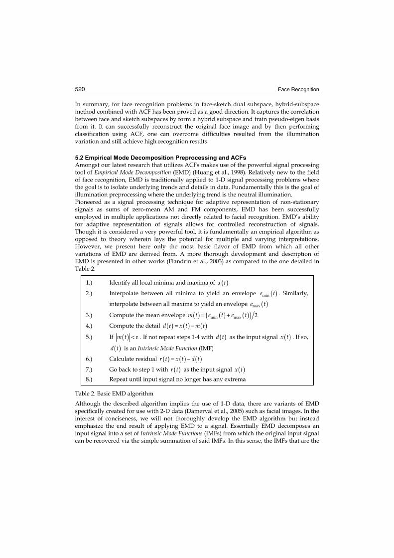
Face Recognition 520
In summary, for face recognition problems in face-sketch dual subspace, hybrid-subspace method combined with ACF has been proved as a good direction. It captures the correlation between face and sketch subspaces by form a hybrid subspace and train pseudo-eigen basis from it. It can successfully reconstruct the original face image and by then performing classification using ACF, one can overcome difficulties resulted from the illumination variation and still achieve high recognition results.
5.2 Empirical Mode Decomposition Preprocessing and ACFs
Amongst our latest research that utilizes ACFs makes use of the powerful signal processing tool of Empirical Mode Decomposition (EMD) (Huang et al., 1998). Relatively new to the field of face recognition, EMD is traditionally applied to 1-D signal processing problems where the goal is to isolate underlying trends and details in data. Fundamentally this is the goal of illumination preprocessing where the underlying trend is the neutral illumination. Pioneered as a signal processing technique for adaptive representation of non-stationary signals as sums of zero-mean AM and FM components, EMD has been successfully employed in multiple applications not directly related to facial recognition. EMD’s ability for adaptive representation of signals allows for controlled reconstruction of signals. Though it is considered a very powerful tool, it is fundamentally an empirical algorithm as opposed to theory wherein lays the potential for multiple and varying interpretations. However, we present here only the most basic flavor of EMD from which all other variations of EMD are derived from. A more thorough development and description of EMD is presented in other works (Flandrin et al., 2003) as compared to the one detailed in Table 2.
Table 2. Basic EMD algorithm
Although the described algorithm implies the use of 1-D data, there are variants of EMD specifically created for use with 2-D data (Damerval et al., 2005) such as facial images. In the interest of conciseness, we will not thoroughly develop the EMD algorithm but instead emphasize the end result of applying EMD to a signal. Essentially EMD decomposes an input signal into a set of Intrinsic Mode Functions (IMFs) from which the original input signal can be recovered via the simple summation of said IMFs. In this sense, the IMFs that are the
1.) Identify all local minima and maxima of ( )x t
2.) Interpolate between all minima to yield an envelope ( )mine t . Similarly,
interpolate between all maxima to yield an envelope ( )maxe t
3.) Compute the mean envelope ( ) ( ) ( )( )min max 2m t e t e t= +
4.) Compute the detail ( ) ( ) ( )d t x t m t= −
5.) If ( )m t < . If not repeat steps 1-4 with ( )d t as the input signal ( )x t . If so,
( )d t is an Intrinsic Mode Function (IMF)
6.) Calculate residual ( ) ( ) ( )r t x t d t= −
7.) Go back to step 1 with ( )r t as the input signal ( )x t8.) Repeat until input signal no longer has any extrema

Frequency Domain Face Recognition 521
result of application of EMD to a signal can be thought of as a series of basis signals for the input signal. Using EMD as a preprocessing tool, we can decompose facial images into their IMFs or basis images of which a few will contain the majority of illumination effects. Reconstruction of the original facial image sans these illumination-variant IMFs will yield a more illumination-neutral image from which more accurate recognition can be performed (Bhagavatula & Savvides, 2007).
(a) (b) Figure 13. Result of EMD preprocessing on an image taken from the PIE No-Lights face database (a) Prior to EMD preprocessing (b) After EMD preprocessing
Figure 14. IMFs created from applying EMD to the face image in Figure 13 (a)
As Figure 13 demonstrates, EMD preprocessing is capable of removing cast shadow effects while retaining the majority of useful information. Although the image in Figure 13 (b) appears discolored, it is a far better image to perform face recognition on than the original image presented in Figure 13 (a). To further illustrate this point we present in Figure 14 the IMFs decomposed from the image in Figure 13 (a). Taking note of the last IMF, we can clearly see the overall effect of the cast shadow in this IMF and can intuitively appreciate the effect of reconstructing the facial image minus this particular IMF. We show in Figure 15 the average performance of ACFs prior to and after EMD preprocessing on the Carnegie Mellon University Pose-Illumination-Expression (CMU PIE) No-Lights face database (Sims et al, 2003). Our results indicate that although ACFs perform exceedingly well even under illumination-variant conditions, their performance does benefit from some illumination normalization as is provided by EMD preprocessing. These results not only underscore the power of ACFs but also that of EMD which as signal decomposition tool which effectively yields AM and FM components of a signal is also a frequency domain processing technique. With both these algorithms available to us, we are capable of achieving significantly accurate face recognition in illumination-variant conditions.

Face Recognition 522
Figure 15. Average EERs comparing performance of ACFs prior to and after EMD preprocessing
6. Conclusions and Future Work
We have shown through the course of this chapter that the Fourier or frequency domain of facial data contains significantly more useful information when processed than its spatial counterpart. The simple coupling of standard algorithms such as Eigenfaces and Fisherfaceswith frequency domain representation of phase and magnitude spectrums, can result in noticeable improvements in performance as we have shown for pose and illumination tolerance. Evolving our intuition about the frequency domain leads us to the group of algorithms collectively referred as ACFs. Primarily originating from frequency domain interpretations of data, ACFs allow for significant discriminative ability while providing other attractive qualities such as shift invariance, noise tolerance, and graceful degredation. As the presented results indicate, ACFs are capable of performing highly accurate face recognition in varying and challenging circumstances. In particular, the presented work also demonstrates the compatibility of ACFs with other algorithms allowing them to be easily integrated into most face recognition systems. Frequency domain related algorithms, particularly ACFs, still hold much potential in advancing the area of face recognition and biometrics in general. Our proposed future work spans the broad horizon of face recognition including but not limited to improved general face recognition, large scale applications, improved illumination tolerance, hardware implementations, and privacy issues. The last area mentioned holds great significance in today’s digital world. Although biometrics are gaining popularity as a reliable and secure method of authentication and identification, they are as susceptible to loss as typical ciphers or passwords. Represented as digital data, a biometric template can be stolen and as an almost unique identifier of a person cannot be replaced. To this end, cancellable biometrics are being developed to allow re-usability and re-issuement of biometrics using encryption type methods and performing the recognition in the encrypted domain. ACFs easily integrate into the scheme of cancellable biometrics (Jain & Uludag, 2003; Savvides et al.,

Frequency Domain Face Recognition 523
2004c, 2004e; Ratha et al., 2006). This research is amongst the most pressing as widespread acceptance of face recognition is contingent on allaying these privacy concerns. Face recognition research and technology has made significant progress over the last decade. Advances in recognition algorithms have enabled some headway into commercially viable systems. However, performance is still considered lacking with respect to the need for reliable and accurate identification. Our research into frequency domain algorithms is but one of many approaches to this problem. However, unlike other approaches, ours’ is relatively unique and offers a great potential for improvement with the designed distortion tolerance and shift-invariance. We intend to continue with our research in frequency domain face recognition exploiting and analyzing all aspects of the frequency content of useful for identifying human faces.
7. References
Bhagavatula, R. & Savvides, M. (2005a) Eigen and Fisher-Fourier spectra for shift invariant pose-tolerant face recognition. Proceedings of International Conference on Advances in Pattern Recognition, 2005, pp. II-351 - II-359, Bath (UK), Aug. 2005, Springer
Bhagavatula, R. & Savvides, M. (2005b) PCA vs. automatically pruned wavelet-packet PCA for illumination tolerant face recognition. Proceedings of IEEE Workshop on Automatic Identification Advanced Technologies, 2005, pp. 69 - 74, Buffalo, NY (USA), Oct. 2005, IEEE
Bhagavatula, R. & Savvides, M. (2007) Empirical mode decomposition for removal of specular reflections and cast shadow effects. Proceedings of SPIE Defense and Security Symposium, 2007, (pending publication), Orlando, FL (USA), April 2007, SPIE
Belhumeur, P.N.; Hespanha, J.P. & Kreigman, D.J. (1997) Eigenfaces vs. Fisherfaces: recognition using class specific linear projection. IEEE Transactions on Pattern Analysis and Machine Intelligence, Vol. 19, No. 7, July 1997, pp. 711 - 720
Chen, T.; Hsu, Y.J.; Liu, X. & Whang, W. (2002) Principle component analysis and its variants for biometrics. Proceedings of IEEE International Conference on Image Processing, 2002, pp. I-61 - I-64, Rochester, NY (USA), Sept. 2002, IEEE
Chellappa, R.; Wilson, C.L. & Sirohey, S. (1995) Human and machine recognition of faces: a survey. Proceedings of the IEEE, Vol. 83, No. 5, May 1995, pp. 705 - 741
Damerval, C.; Meignen, S. & Perrier, V. (2005) A fast algorithm for bidimensional EMD. IEEE Signal Processing Letters, Vol. 12, No. 10, Oct. 2005, pp. 701 - 704
Flandrin, P.; Goncalves, P. & Rilling, G. (2003) On empirical mode decomposition and its algorithms. Proceedings of IEEE-EURASIP Workshop on Nonlinear Signal and Image Processing, 2003, Grod-Trieste (Italy), June 2003, IEEE
Fisher, R. (1936). The use of multiple measures in taxonomic problems. Ann. Eugenics, Vol. 7, 1936, pp. 179-188
Grudin, M.A. (2000) On internal representation in face recognition systems. Pattern Recognition, Vol. 33, No. 7, 2000, pp. 1161 - 1177
Hayes, M.H; Lim, J.S & Oppenheim, A.V (1980) Signal reconstruction from phase or magnitude. IEEE Transactions on Acoustics and Signal Processing, Vol. 28, Dec 1980, pp 672 - 680

Face Recognition 524
Huang, N.E.; Shen, Z.; Long, S.R.; Wu, M.L.; Shih, H.H.; Zheng, Q.; Yen, N.C.; Tung C.C., & Liu, H.H. (1998) The empirical mode decomposition and Hilbert spectrum for nonlinear and non-stationary time series analysis. Proceedings Royal Society London,Vol. 454, 1998, pp. 903 - 995
Heo, J.; Savvides, M. & Vijaya Kumar, B.V.K. (2005) Performance evaluation of face recognition using visual and thermal imagery with advanced correlation filters. Proceedings IEEE International Conference on Computer Vision and Pattern Recognition, 2005, pp. III-9 - III-14, San Diego, CA (USA), June 2005, IEEE
Heo, J.; Savvides, M.; Abiantun, R.; Xie, C. & Vijaya Kumar, B.V.K. (2006) Face recognition with kernel correlation filters on a large scale database. Proceedings of IEEE International Conference on Acoustics, Speech and Signal Processing, 2006, pp. II-181 - II-184, Toulouse (France), May 2006, IEEE
Hester, C. & Casasent, D. (1980) Multivariant technique for multiclass pattern recognition. Applied Optics, Vol. 19, No. 11, June 1980, pp.1758 - 1761
Jain, A.K. & Uludag, U. (2003) Hiding biometric data. IEEE Transactions on Pattern Analysis and Machine Intelligence, Vol. 25, No. 11, Nov. 2003, pp. 1494 - 1498
Li, Y.; Savvides, M. & Vijaya Kumar, B.V.K. (2006). Illumination tolerant face recognition using a novel face from sketch synthesis approach and advanced correlation filters. Proceedings of IEEE International Conference on Acoustics, Speech and Signal Processing, 2006, pp. II-357 - II-360, Toulouse (France), May 2006, IEEE
Mahalanobis, A.; Vijaya Kumar, B.V.K. & Casasent, D. (1987). Minimum average correlation energy filters. Applied Optics, Vol. 26, Issue 17, Sept., 1987, pp. 3633 - 3640
Mahalanobis, A.; Vijaya Kumar, B.V.K.; Song, S.; Sims, S.R.F. & Epperson, J.F. (1994). Unconstrained correlation filters. Applied Optics, Vol. 33, No. 17, June 1994, pp. 3751 - 3759
Ng, C.K.; Savvides, M. & Khosla, P.K. (2005) Real-time face verification on a cell-phone using advanced correlation filters. Proceedings of IEEE Workshop on Automatic Identification Advanced Technologies, 2005, pp. 57 - 62, Buffalo, NY (USA), Oct. 2005, IEEE
Oppenheim, A.V & Lim, J.S. (1981). The importance of phase in signals. Proceedings of the IEEE Vol. 69, No. 5, May 1981, pp 529 - 541
Phillips, P.J.; Moon, H.; Rizvi, S.A. & Rauss P.J. (2000) The FERET evaluation methodology for face-recognition algorithms. IEEE Transactions on Pattern Analysis and Machine Intelligence, Vol. 22, No. 10, Oct. 2000, pp. 1090 - 1104
Phillips, P.J.; Grother, P.; Micheals, R.; Blackburn, D.M.; Tabassi, E. & Bone, M. (2003) Face recognition vendor test 2002. Proceedings of IEEE International Workshop on Analysis and Modeling of Faces and Gestures, 2003, pp. 44, Nice (France), Oct. 2003, IEEE
Phillips, P.J.; Flynn, P.J.; Scruggs, T.; Bowyer, K.W.; Chang, J.; Hoffman, K.; Marques, J.; Min, J. & Worek, W. (2005) Overview of the face recognition grand challenge. Proceedings of IEEE International Conference on Computer Vision and Pattern Recognition, 2005, pp. I-947 - I-954, San Diego, CA (USA), June 2005, IEEE
Ratha, N.; Connell, J.; Bolle, R.N. & Chikkerur, S. (2006) Cancelable biometrics: a case study in fingerprints. Proceedings of IEEE International Conference on Pattern Recognition, 2006, pp. IV-370 - IV-373, Hong Kong (China), Aug. 2006, IEEE

Frequency Domain Face Recognition 525
Savvides, M.; Vijaya Kumar, B.V.K. & Khosla P.K. (2002) Two-class minimax distance transform correlation filter. Applied Optics, Vol. 31, No. 32, Nov. 2002, pp. 6829 - 6840
Savvides, M. & Vijaya Kumar (2003a) Illumination normalization using logarithm transforms for face authentication. Proceedings of International Conference on Advances in Pattern Recognition, 2003, pp. 549 - 556, Guildford (UK), June 2003, Springer
Savvides, M. & Vijaya Kumar (2003b) Quad phase minimum average correlation energy filters for reduced memory illumination tolerant face authentication. Proceedings of International Conference on Advances in Pattern Recognition, 2003, pp. 19 - 26, Guildford (UK), June 2003, Springer
Savvides, M.; Venkataramani & Vijaya Kumar, B.V.K. (2003c) Incremental updating of advanced correlation filters for biometric authentication systems. Proceedings of IEEE International Conference on Multimedia and Expo, 2003, pp. III-229 - III-232, Baltimore, MD (USA), July 2003, IEEE
Savvides, M.; Vijaya Kumar, B.V.K. & Khosla, P.K. (2004a) “Corefaces“ - robust shift invariant PCA based correlation filter for illumination tolerant face recognition. Proceedings of IEEE International Conference on Computer Vision and Pattern Recognition, 2004, pp. II-834 - II-841, Washington, DC (USA), July 2004, IEEE
Savvides, M.; Vijaya Kumar, B.V.K. & Khosla, P.K. (2004b) Eigenphases vs. Eigenfaces. Proceedings of IEEE International Conference on Pattern Recognition, 2004, pp. III-810 - III-813, Cambridge (UK), Aug. 2004, IEEE
Savvides, M. & Vijaya Kumar, B.V.K. (2004c) Cancellable biometric filters for face recognition. Proceedings of IEEE International Conference on Pattern Recognition, 2004,pp. III-922 - III-925, Cambridge (UK), Aug. 2004, IEEE
Savvides, M.; Vijaya Kumar, B.V.K. & Khosla P.K. (2004d) Robust shift invariant biometric identification from partial face images. Proceedings of SPIE Defense and Security Symposium, 2004, pp. 124 - 135, Orlando, FL (USA), Aug. 2004, SPIE
Savvides, M.; Vijaya Kumar, B.V.K. & Khosla, P.K. (2004e) Authentication invariant cancellable correlation filters for illumination tolerant face recognition. Proceedings of SPIE Defense and Security Symposium, 2004, pp. 156 - 163, Orlando, FL (USA), Aug. 2004, SPIE
Savvides, M.; Vijaya Kumar, B.V.K. & Khosla P.K. (2004f) Illumination tolerant face recognition using advanced correlation filters trained from a single image. Presented at the Biometrics Consortium, 2004, Crystal City, VA (USA), 2004
Savvides, M.; Heo, J.; Abiantun, R.; Xie, C. & Vijaya Kumar, B.V.K. (2006a) Class dependent kernel discrete cosine transform features for enhanced holistic face recognition in FRGC-II. Proceedings of IEEE International Conference on Acoustics, Speech and Signal Processing, 2006, pp. II-185 - II-188, Toulouse (France), May 2006, IEEE
Savvides, M.; Heo, J.; Abiantun, R.; Xie, C. & Vijaya Kumar, B.V.K. (2006b) Partial and holistic face recognition on FRGC-II data using support vector machines. Proceedings of IEEE International Conference on Computer Vision and Pattern Recognition, 2006, pp. 48 - 53, New York, NY (USA), June 2006, IEEE
Sim, T.; Baker, S. & Bsat, M. (2003) The CMU pose, illumination, and expression database. IEEE Transactions on Pattern Analysis and Machine Intelligence, Vol. 25, No. 12, Dec. 2003, pp. 1615 - 1618

Face Recognition 526
Swets, D.L. & Weng, J. (1996) Discriminant analysis and eigenspace partition tree for face and object recognition from view. Proceedings of IEEE International Conference on Automatic Face and Gesture Recognition, 1996, pp. 192 - 197, Killington, VT (USA), Oct. 1996, IEEE
Tang, X. & Wang X. (2002). Face photo recognition using sketch. Proceedings of IEEE International Conference on Image Processing, 2002, pp. I-257 - I-260, Rochester, NY (USA), Sept. 2002, IEEE
Turk, M.A. & Pentland, A.P. (1991) Face recogntion using eigenfaces. Proceedings of IEEE International Conference on Computer Vision and Pattern Recognition, 1991, pp. 589 - 591, June 1991, IEEE
Vijaya Kumar, B.V.K. (1986). Minimum variance synthetic discriminant functions. Journal of the Optical Society of America, Vol. 3, No. 10, Oct. 1986, pp. 1579 - 1584
Vijaya Kumar, B.V.K. (1992). Tutorial survey of composite filter designs for optical correlators. Applied Optics, Vol. 31, No. 23, Aug. 1992, pp. 4773 - 4801
Vijaya Kumar, B.V.K.; Carlson, D. & Mahalanobis, A. (1994). Optimal tradeoff synthetic discriminant function (OTSDF) filters for arbitrary devices. Optics Letters, Vol. 19, No. 19, Oct. 1994, pp. 1556 - 1558
Vijaya Kumar, B.V.K.; Mahalanobis, A. & Juday, R. (2005) Correlation Pattern Recognition,Cambridge University Press, 13 978-0-521-57103-6, New York, NY (USA)
Vijaya Kumar, B.V.K.; Savvides, M. & Xie, C. (2006) Correlation pattern recognition for face recognition. Proceedings of the IEEE, Vol. 94, No. 11, Nov. 2006, pp 1963 - 1976
Yang, J.; Zhang, D.; Frangi, A.F. & Yang, J. (2004) Two-dimensional PCA: a new approach to appearance-based face recognition and recognition, IEEE Transactions on Pattern Analysis and Machine Intelligence, Vol. 26, Issue 1, Jan. 2004, pp. 131 - 137
Zhao, W.; Chellappa, R. & Krishnaswamy, A. (1998) Discriminant analysis of princpal components for face recognition. Proceedings of IEEE International Conference on Automatic Face and Gesture Recognition, 1998, pp 336 - 341, Nara (Japan), April 1998, IEEE
Zhao, W.; Chellappa, R. & Phillips, P.J. (1999) Subspace linear discriminant analysis for face recognition. Technical Report CAR-TR-914, 1999
Zhao, W.; Chellappa, R.; Phillips, P.J. & Rosenfield, A. (2003) Face recognition: a literature survey. Association for Computer Machinery Computing Surveys, Vol. 35, No. 4, Dec. 2003, pp. 399 - 458
27
From Canonical Face to Synthesis – An Illumination Invariant Face Recognition
Approach
Tele Tan Curtin University of Technology
Australia
1. Introduction
The need to further develop robust face recognition techniques to meet real world requirements is still an open research challenge. It is widely understood that the two main contributions of poor recognition performances are that caused by variations in face pose and lighting. We will deal with the problem of illumination in this chapter. Approaches addressing the illumination-related problems can be broadly classified into two categories; feature-based approach and exemplar- or appearance- based approach. Feature-based approaches aim to define a feature space that exhibits some broad invariance over the lighting variations. Examples of these are (Adini & Ullman, 1997), (Belhumeur et al., 1997) and (Yang et al., 2004) which uses different image representations like 2D Gabor-like filters, first and second derivatives of the image, and the logarithmic transformation. Although these features may exhibit intensity immunity, none of these are found to be reliable to cope with significantly large variations in illumination changes (Manjunath et al.1992) (Yang et al., 2004). Exemplar- or appearance- based approaches use a set of sample images taken of a class object (in this case a face) as a basis to compute an intermediary image. The intermediate image can then be used either directly as the probe image or be used to synthesize novel views of the face under different lighting conditions (Mariani, 2002). For example, (Riklin-Raviv & Shashua, 2001) reported a method to compute the Quotient Image from a small sample of bootstrap images representing a minimum of two class objects. The illumination invariant signature of the Quotient Image enables an analytic generation of the novel image space with varying illumination. However, this technique is highly dependent on the types of bootstrap images used which has the undesirable effect of generating diversely looking Quotient Images even from the same person. (Sim & Kanade, 2001) used a statistical shape-from-shading model to estimate the 3D face shape from a single image. The 3D recovery model is based on the symmetric shape-from-shading algorithm proposed by (Zhao & Chellappa, 1999). They used the 3D face model to synthesize novel faces under new illumination conditions using computer graphics algorithms. The approach produce high recognition rate on the illumination subset of the CMU PIE database (Sim et al., 2003). However, it was not evident how their synthesis technique can cope with extreme illumination conditions (Sim & Kanade, 2001). (Debevec et al., 2000) presented a method to

Face Recognition 528
acquire the reflectance field of a human face and use these measurements to render the face under arbitrary changes in lighting and viewpoint. However, the need to generate a large sample of images using the light stage is unfeasible for face recognition purposes. A parameter-free method of estimating the bi-directional reflectance distribution of a subject’s skin was proposed by (Smith et al., 2004). They estimated the radiance function by exploiting differential geometry and making use of the Gauss map from the surface onto a unit sphere. They demonstrated the approach by applying it to the re-rendering of faces with different skin reflectance models. As in (Riklin-Raviv & Shashua, 2001) and (Mariani, 2002), we address the problem of class-based image synthesis and recognition with varying illumination conditions. We define an ideal class as a collection of 3D objects that have approximately the same shape but different albedo functions. For recognition purposes, we can broadly assume all human faces to belong to a certain class structure. This assumption was similarly adopted by (Riklin-Raviv & Shashua, 2001) and (Mariani, 2002). Our approach is based on the dual recovery of the canonical face model and lighting models given a set of images taken with varying lighting conditions and from a minimum of two distinct subjects within the class. The canonical image is equivalent to the reflectance field of the face that is invariant to illumination. The lighting model is the image representation of the ambient lighting independent of the face input. We will first formulate the problem with an over-determined set of equations and propose a method in solving them over every pixel location in the image. We will demonstrate the quality of the recovered canonical face for generating novel appearances using both subjective and objective measures.
2. The Illumination Model
The intensity of reflected light at a point on a surface is the integral over the hemisphere above the surface of a light function L times a reflectance function R. The pixel equation at point (x,y,z) can be expressed as
ttRzyxtLzyxI
t
dddd),,,(),,,,,,(),,( λφθλφθλφθ
λθ φ
= (1)
wherex,y,z = the co-ordinate of the point on the surface φ and θ = azimuth and yaw angle from the z axis respectively t and λ = time and wavelength of the light source
This equation is computationally too complex to solve in many real-time applications. We need to make further simplification of the equation without significantly affecting the goal of our work. Firstly, z, t and λ can be eliminated because we are dealing with the projected intensity value of a 3D point onto a single frame grey scale digital image. Additionally, if one considers fixing the relative location of the camera and the light source, θ and φ both become constants and the reflectance function collapses to point (x, y) in the image plane. This is a valid condition since we assume the camera to be positioned directly in front of the human subject at all times. Therefore, the first-order approximation of equation (1) for a digital image I(x,y) can be further written as:
I(x,y) R(x,y) L(x,y) (2)

From Canonical Face to Synthesis – An Illumination Invariant Face Recognition Approach 529
where R(x,y) is the reflectance and L(x,y) is the illumination at each image sample point (x,y).Our approach is to use exemplar images taken over different fixed lighting directions to recover both the reflectance model and illumination source at the same time. It is not the scope of this work to accurately model the skin reflectance property according to specificity like the melanin content of the skin, skin haemoglobin concentration and level of perspirations. These are important for visually accurate skin rendering application but less so for face recognition purposes.
3. Computing the Canonical Face and the Illumination Models
In our case, only the measured intensity images are available. Therefore, there are twice as many unknown data (RHS) as there are known data (LHS) making equation (2) ill-posed. The reflectance surface essentially comprises the combination of the reflectance property associated with the pigmentation of the skin, mouth, eyes and artifacts like facial hair. We define the reflectance model as the canonical face and represent it as a grey level intensity image. We will formulate the dual recovery technique for the canonical faces and illumination models given a set of intensity images Iij(x,y) Rj(x,y) Li(x,y), where i and j are indices to the collection of bootstrap1 faces taken from M distinct persons (j = 1, ..., M) and N different lighting directions (i = 1, ..., N).
3.1 Defining and Solving the Systems of Equations
As explained in the previous section, equation (2) has more unknown terms than known. In order to make the equation solvable in a least square sense, we need to introduce additional measurements thus making the system of equations over determined. We further note that the bootstrap image, Iij(x,y) has two variable components. They are the reflectance component which is unique to the individual person and the illumination model which is dependent on the lighting source and direction. Suppose we have M distinct persons which we use in the bootstrap collection (i.e. Rj, j = 1, …, M) and N spatially distributed illumination sources whose direction with respect to the person is fixed at all instances (i.e. Li, i = 1, …, N), we will have therefore a total of MxN known terms and M+N unknown terms. These over-determined systems of equations can be solved by selecting any values of M and N that are greater than 1. For example, if we use M persons from the bootstrap collection, and collect N images for each person by varying the illumination, we get the following system of equations;
Ii1(x,y) R1(x,y) Li(x,y) (3)
IiM(x,y) RM(x,y) Li(x,y)
where i = 1,…,N. The terms on the left hand side of these equations are the bootstrap images from the M number of persons. If the illuminations used to generate these bootstrap images are the same, the illumination models, Li will be common for every person as is reflected in equation (3).
1 The bootstrap collection comprises of face sample images taken of various person over multiple
illumination directions, the relative location of which are fixed.
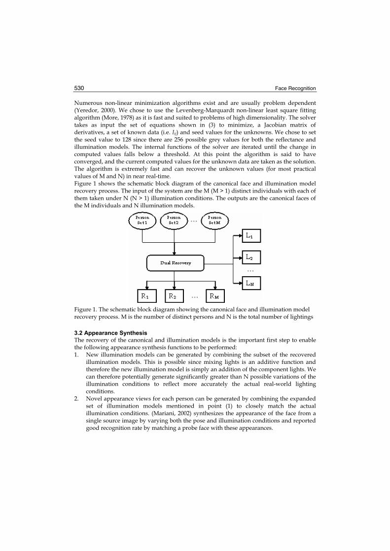
Face Recognition 530
Numerous non-linear minimization algorithms exist and are usually problem dependent (Yeredor, 2000). We chose to use the Levenberg-Marquardt non-linear least square fitting algorithm (More, 1978) as it is fast and suited to problems of high dimensionality. The solver takes as input the set of equations shown in (3) to minimize, a Jacobian matrix of derivatives, a set of known data (i.e. Iij) and seed values for the unknowns. We chose to set the seed value to 128 since there are 256 possible grey values for both the reflectance and illumination models. The internal functions of the solver are iterated until the change in computed values falls below a threshold. At this point the algorithm is said to have converged, and the current computed values for the unknown data are taken as the solution. The algorithm is extremely fast and can recover the unknown values (for most practical values of M and N) in near real-time. Figure 1 shows the schematic block diagram of the canonical face and illumination model recovery process. The input of the system are the M (M > 1) distinct individuals with each of them taken under N (N > 1) illumination conditions. The outputs are the canonical faces of the M individuals and N illumination models.
Figure 1. The schematic block diagram showing the canonical face and illumination model recovery process. M is the number of distinct persons and N is the total number of lightings
3.2 Appearance Synthesis
The recovery of the canonical and illumination models is the important first step to enable the following appearance synthesis functions to be performed: 1. New illumination models can be generated by combining the subset of the recovered
illumination models. This is possible since mixing lights is an additive function and therefore the new illumination model is simply an addition of the component lights. We can therefore potentially generate significantly greater than N possible variations of the illumination conditions to reflect more accurately the actual real-world lighting conditions.
2. Novel appearance views for each person can be generated by combining the expanded set of illumination models mentioned in point (1) to closely match the actual illumination conditions. (Mariani, 2002) synthesizes the appearance of the face from a single source image by varying both the pose and illumination conditions and reported good recognition rate by matching a probe face with these appearances.
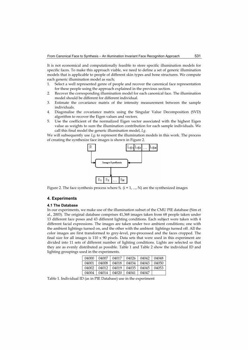
From Canonical Face to Synthesis – An Illumination Invariant Face Recognition Approach 531
It is not economical and computationally feasible to store specific illumination models for specific faces. To make this approach viable, we need to define a set of generic illumination models that is applicable to people of different skin types and bone structures. We compute each generic illumination model as such; 1. Select a well represented genre of people and recover the canonical face representation
for these people using the approach explained in the previous section. 2. Recover the corresponding illumination model for each canonical face. The illumination
model should be different for different individual. 3. Estimate the covariance matrix of the intensity measurement between the sample
individuals. 4. Diagonalise the covariance matrix using the Singular Value Decomposition (SVD)
algorithm to recover the Eigen values and vectors. 5. Use the coefficient of the normalized Eigen vector associated with the highest Eigen
value as weights to sum the illumination contribution for each sample individuals. We call this final model the generic illumination model, Lg.
We will subsequently use Lgi to represent the illumination models in this work. The process of creating the synthesize face images is shown in Figure 2.
Figure 2. The face synthesis process where Si (i = 1, ..., N) are the synthesized images
4. Experiments
4.1 The Database
In our experiments, we make use of the illumination subset of the CMU PIE database (Sim et al., 2003). The original database comprises 41,368 images taken from 68 people taken under 13 different face poses and 43 different lighting conditions. Each subject were taken with 4 different facial expressions. The images are taken under two ambient conditions; one with the ambient lightings turned on, and the other with the ambient lightings turned off. All the color images are first transformed to grey-level, pre-processed and the faces cropped. The final size for all images is 110 x 90 pixels. Data sets that were used in this experiment are divided into 11 sets of different number of lighting conditions. Lights are selected so that they are as evenly distributed as possible. Table 1 and Table 2 show the individual ID and lighting groupings used in the experiments.
04000 04007 04017 04026 04042 0404804001 04008 04018 04034 04043 0405004002 04012 04019 04035 04045 0405304004 04014 04020 04041 04047
Table 1. Individual ID (as in PIE Database) use in the experiment
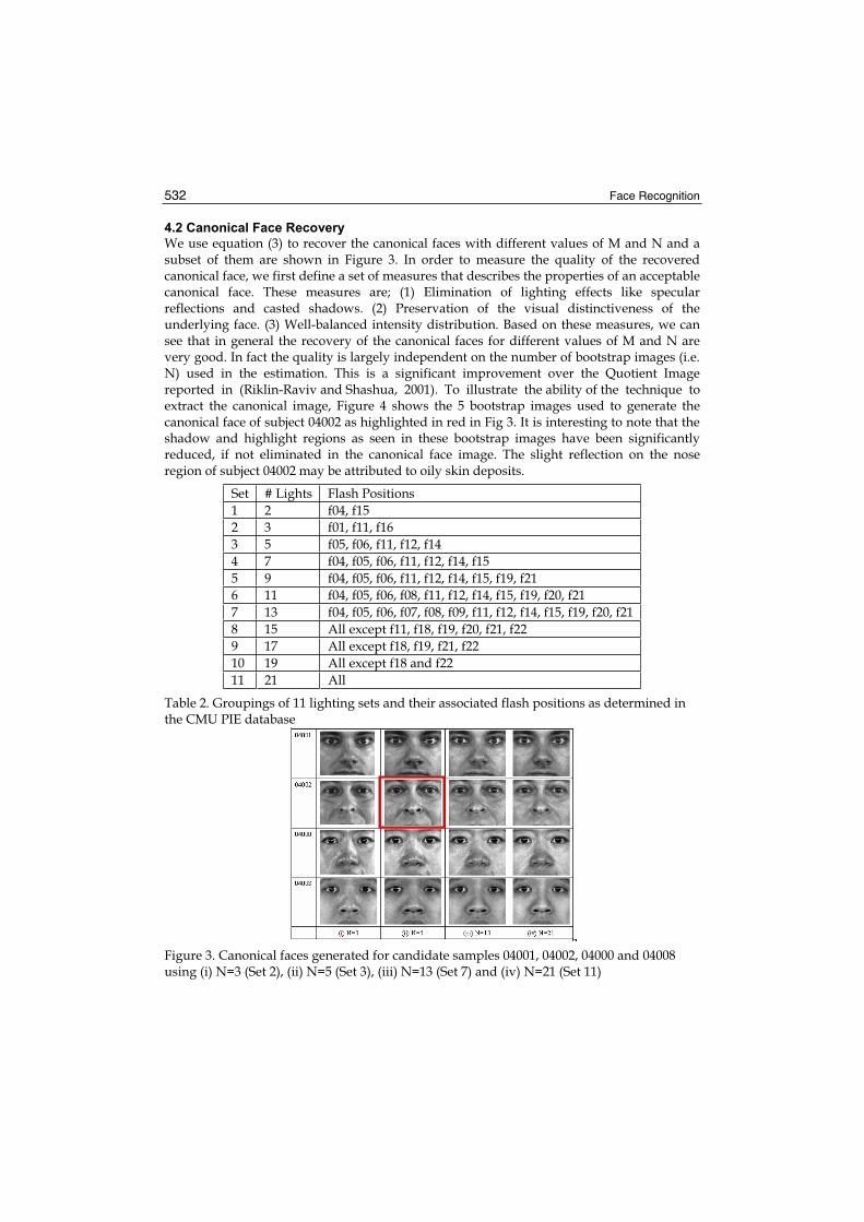
Face Recognition 532
4.2 Canonical Face Recovery
We use equation (3) to recover the canonical faces with different values of M and N and a subset of them are shown in Figure 3. In order to measure the quality of the recovered canonical face, we first define a set of measures that describes the properties of an acceptable canonical face. These measures are; (1) Elimination of lighting effects like specular reflections and casted shadows. (2) Preservation of the visual distinctiveness of the underlying face. (3) Well-balanced intensity distribution. Based on these measures, we can see that in general the recovery of the canonical faces for different values of M and N are very good. In fact the quality is largely independent on the number of bootstrap images (i.e. N) used in the estimation. This is a significant improvement over the Quotient Image reported in (Riklin-Raviv and Shashua, 2001). To illustrate the ability of the technique to extract the canonical image, Figure 4 shows the 5 bootstrap images used to generate the canonical face of subject 04002 as highlighted in red in Fig 3. It is interesting to note that the shadow and highlight regions as seen in these bootstrap images have been significantly reduced, if not eliminated in the canonical face image. The slight reflection on the nose region of subject 04002 may be attributed to oily skin deposits.
Set # Lights Flash Positions 1 2 f04, f15 2 3 f01, f11, f16 3 5 f05, f06, f11, f12, f14 4 7 f04, f05, f06, f11, f12, f14, f15 5 9 f04, f05, f06, f11, f12, f14, f15, f19, f21 6 11 f04, f05, f06, f08, f11, f12, f14, f15, f19, f20, f21 7 13 f04, f05, f06, f07, f08, f09, f11, f12, f14, f15, f19, f20, f21 8 15 All except f11, f18, f19, f20, f21, f22 9 17 All except f18, f19, f21, f22 10 19 All except f18 and f22 11 21 All
Table 2. Groupings of 11 lighting sets and their associated flash positions as determined in the CMU PIE database
Figure 3. Canonical faces generated for candidate samples 04001, 04002, 04000 and 04008 using (i) N=3 (Set 2), (ii) N=5 (Set 3), (iii) N=13 (Set 7) and (iv) N=21 (Set 11)
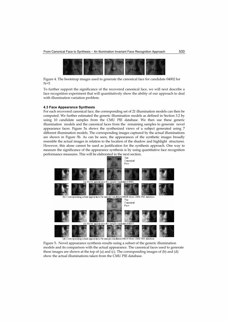
From Canonical Face to Synthesis – An Illumination Invariant Face Recognition Approach 533
Figure 4. The bootstrap images used to generate the canonical face for candidate 04002 for N=5
To further support the significance of the recovered canonical face, we will next describe a face recognition experiment that will quantitatively show the ability of our approach to deal with illumination variation problem.
4.3 Face Appearance Synthesis
For each recovered canonical face, the corresponding set of 21 illumination models can then be computed. We further estimated the generic illumination models as defined in Section 3.2 by using 10 candidate samples from the CMU PIE database. We then use these generic illumination models and the canonical faces from the remaining samples to generate novel appearance faces. Figure 5a shows the synthesized views of a subject generated using 7 different illumination models. The corresponding images captured by the actual illuminations are shown in Figure 5b. As can be seen, the appearances of the synthetic images broadly resemble the actual images in relation to the location of the shadow and highlight structures. However, this alone cannot be used as justification for the synthesis approach. One way to measure the significance of the appearance synthesis is by using quantitative face recognition performance measures. This will be elaborated in the next section.
Figure 5. Novel appearance synthesis results using a subset of the generic illumination models and its comparison with the actual appearance. The canonical faces used to generate these images are shown at the top of (a) and (c). The corresponding images of (b) and (d) show the actual illuminations taken from the CMU PIE database.
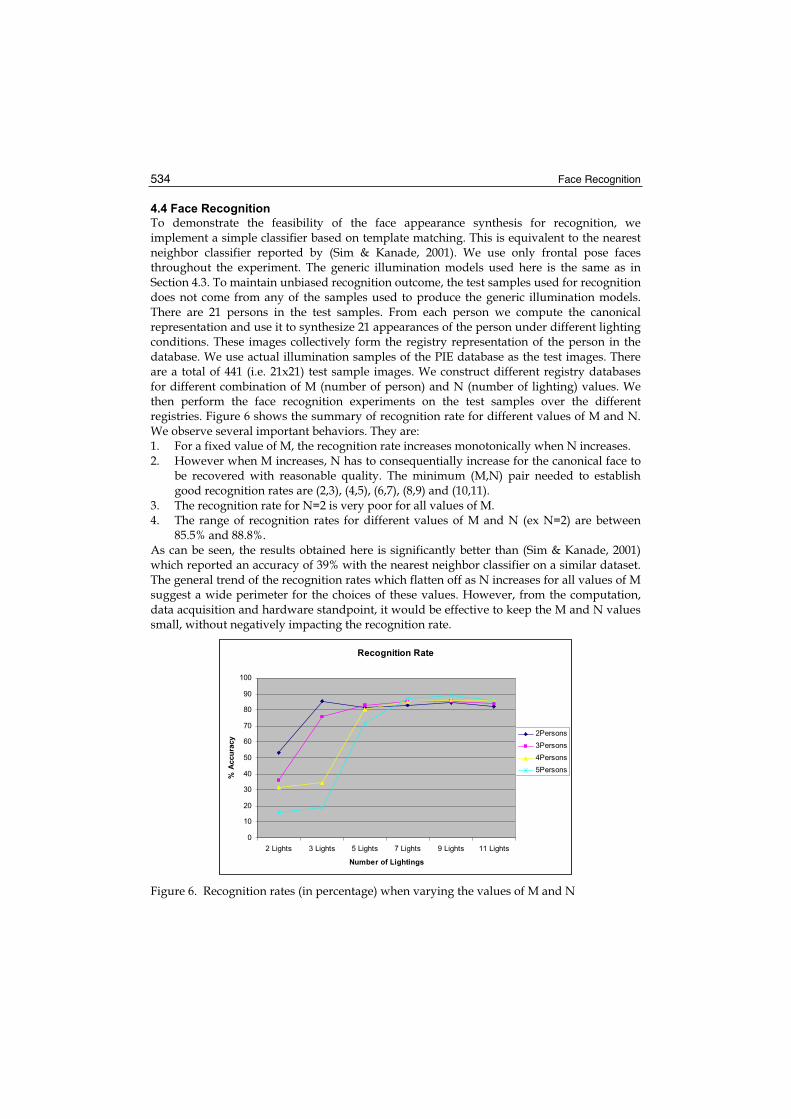
Face Recognition 534
4.4 Face Recognition
To demonstrate the feasibility of the face appearance synthesis for recognition, we implement a simple classifier based on template matching. This is equivalent to the nearest neighbor classifier reported by (Sim & Kanade, 2001). We use only frontal pose faces throughout the experiment. The generic illumination models used here is the same as in Section 4.3. To maintain unbiased recognition outcome, the test samples used for recognition does not come from any of the samples used to produce the generic illumination models. There are 21 persons in the test samples. From each person we compute the canonical representation and use it to synthesize 21 appearances of the person under different lighting conditions. These images collectively form the registry representation of the person in the database. We use actual illumination samples of the PIE database as the test images. There are a total of 441 (i.e. 21x21) test sample images. We construct different registry databases for different combination of M (number of person) and N (number of lighting) values. We then perform the face recognition experiments on the test samples over the different registries. Figure 6 shows the summary of recognition rate for different values of M and N. We observe several important behaviors. They are: 1. For a fixed value of M, the recognition rate increases monotonically when N increases. 2. However when M increases, N has to consequentially increase for the canonical face to
be recovered with reasonable quality. The minimum (M,N) pair needed to establish good recognition rates are (2,3), (4,5), (6,7), (8,9) and (10,11).
3. The recognition rate for N=2 is very poor for all values of M. 4. The range of recognition rates for different values of M and N (ex N=2) are between
85.5% and 88.8%. As can be seen, the results obtained here is significantly better than (Sim & Kanade, 2001) which reported an accuracy of 39% with the nearest neighbor classifier on a similar dataset. The general trend of the recognition rates which flatten off as N increases for all values of M suggest a wide perimeter for the choices of these values. However, from the computation, data acquisition and hardware standpoint, it would be effective to keep the M and N values small, without negatively impacting the recognition rate.
Recognition Rate
0
10
20
30
40
50
60
70
80
90
100
2 Lights 3 Lights 5 Lights 7 Lights 9 Lights 11 Lights
Number of Lightings
% A
ccu
racy
2Persons
3Persons
4Persons
5Persons
Figure 6. Recognition rates (in percentage) when varying the values of M and N

From Canonical Face to Synthesis – An Illumination Invariant Face Recognition Approach 535
5. Discussion
The results obtained using the canonical face recovery algorithm is very encouraging. We have shown that the minimum number of illumination specified bootstrap images (i.e. N) needed to generate a stable canonical face ranges between 3 and 5. This makes good hardware design sense as an elaborate light stage setup (Sim et al., 2003) (Debevec et al., 2000) becomes unnecessary. Currently we are fabricating a low-cost portable light array module used to implement the canonical face recovery. Depending on the role, this lighting module can be embedded into the different stages of the face recognition system. For example, the module can be introduced during the registration stage where the objective is to capture a good quality neutral image of the subject (i.e. its canonical representation) to be registered into the system irregardless of the ambient lighting condition. Another possible use is to incorporate it into the image capture system at the front end of the recognition system. This will ensure that the picture taken and used for matching will not be affected again by external light sources. Besides using the images captured by the lighting module as described here, we can explore using shape-from-shading techniques to recover the 3D shape of the face (Zhao and Chellappa, 1999). The range information will be an added boost to improve on the illumination rendering quality as well as for recognition. Although the illumination models recovered using the CMU PIE database generates 21 different variations they are inadequate as some important lighting directions (i.e. especially those coming from the top) are glaringly missing. We will next consider using computer graphics tools to develop a virtual light stage that has the ability to render any arbitrary lighting conditions on a 3D face. These new variations can then be used to extract finer quality illumination models which in turn can be use to synthesis more realistic novel appearance views. Finally, we will explore how the systems of canonical face recovery and appearance synthesis can play a further role in enhancing the performances of illumination challenged real world analysis systems. One possible use of this would be in the area of improving data acquisition for dermatology-based analysis where maintaining colour integrity of the image taken is extremely important.
6. Conclusion
We have developed an exemplar-based approach aim at recovering the canonical face of a person as well as the lighting models responsble for the input image. The recovery is not dependent on the number of person (i.e. M) and number of lighting positions (i.e. N). In fact, we have demonstrated that a low value of M=2 and N=2 are in fact adequate for most cases to achieve a good recovery outcome. The canonical face can either be use as a probe face for recognition or use as a base image to generate novel appearance models under new illumination conditions. We have shown subjectively that the canonical faces recovered with this approach are very stable and not heavily dependent on the types and numbers of the bootstrap images. The strength of the view synthesis algorithm based on the canonical face was further demonstrated by a series of face recognition tests using the CMU PIE images which yielded a 2.3 times recognition improvement over the existing technique.

Face Recognition 536
7. Acknowledgement
We would like to thank the Robotics Institute, Carnegie Mellon University for providing the PIE database images.
8. References
Adini Y. and Ullman S. (1997). Face Recognition: the Problem of Compensating for Changes in Illumination Direction, in Proc. of IEEE Trans. on PAMI. Vol. 19, No. 7, pp. 721-732.
Belhumeur P., Hespanha J. and Kriegman D. (1997). Eigenfaces vs. Fisherfaces: Recognition Using Class Specific Linear Projection, in Proc. of IEEE Trans. on Pattern Analysis and Machine Intelligence. Vol. 19, No. 7, pp. 711-720.
Debevec P., Hawkins T., Tchou C., Sarokin W., and Sagar M. (2000). Acquiring the Reflectance Field of a Human Face, in Proc. of SIGGRAPH 2000, pp. 145-156.
Manjunath B., Chellappa R. and Malsburg C. (1992). A feature based approach to face recognition, in Proc. of IEEE Computer Society. Confr. On Computer Vision and Pattern Recognition, pp. 373-378.
Mariani R., (2002). A Face Location and Recognition System Based on Tangent Distance, Multimodal Interface for Human-Machine Communication, Vol. 48. Ed. Yuen P., Tang Y. and Wang P., World Scientific, pp 3-31.
More J. (1978). The Levenberg-Marquardt Algorithm: Implementation and Theory, in G. Watson, Ed, Lecture Notes in Mathematics, Springer Verlag, pp. 105-116.
Riklin-Raviv T. and Shashua A. (2001). The Quotient Image: Class based Re-rendering and Recognition with Varying Illuminations, in Proc. of IEEE Trans. on PAMI. Vol. 23, No. 2, pp. 129-139.
Sim T. and Kanade T. (2001). Combining Models and Exemplars for Face Recognition: an Illumination Example, in Proc. of Workshop on Models versus Exemplars in Computer Vision, Dec.
Sim T., Baker S. and Bsat M. (2003). The CMU Pose, Illumination and Expression Database, in Proc. of IEEE Trans. on PAMI, Vol. 25, No. 12, pp. 1615-1618.
Smith W., Robles-Kelly A. and Hancock E. (2004). Skin Reflectance Modelling for Face Recognition, in Proc. of the Int’l Confr. on Pattern Recognition, pp. 210-213.
Yang P., Shan S., Gao W., Li S. and Zhang D. (2004). Face recognition using Ada-boosted Gabor features, FG 2004, pp. 356-360.
Yeredor A. (2000). The Extended Least Squares Criterion: Minimisation Algorithms and Applications, IEEE Trans. on Signal Processing, Vol. 49, No. 1, pp. 74-86.
Zhao W. and Chellappa R. (1999). Robust Face Recognition using Symmetric Shape-from-Shading, Technical Report CARTR-919, Centre for Automation Research, University of Maryland, College Park, MD.
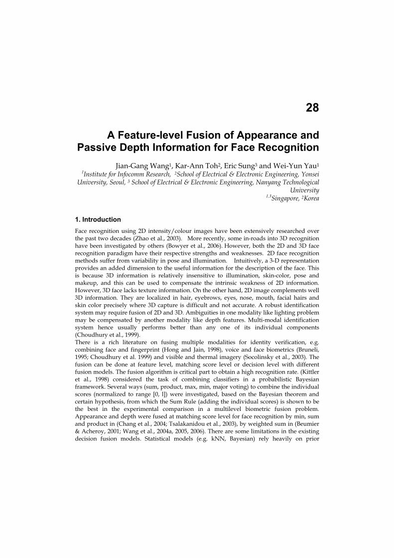
28
A Feature-level Fusion of Appearance and Passive Depth Information for Face Recognition
Jian-Gang Wang1, Kar-Ann Toh2, Eric Sung3 and Wei-Yun Yau11Institute for Infocomm Research, 2School of Electrical & Electronic Engineering, Yonsei
University, Seoul, 3 School of Electrical & Electronic Engineering, Nanyang Technological University
1,3Singapore, 2Korea
1. Introduction
Face recognition using 2D intensity/colour images have been extensively researched over the past two decades (Zhao et al., 2003). More recently, some in-roads into 3D recognition have been investigated by others (Bowyer et al., 2006). However, both the 2D and 3D face recognition paradigm have their respective strengths and weaknesses. 2D face recognition methods suffer from variability in pose and illumination. Intuitively, a 3-D representation provides an added dimension to the useful information for the description of the face. This is because 3D information is relatively insensitive to illumination, skin-color, pose and makeup, and this can be used to compensate the intrinsic weakness of 2D information. However, 3D face lacks texture information. On the other hand, 2D image complements well 3D information. They are localized in hair, eyebrows, eyes, nose, mouth, facial hairs and skin color precisely where 3D capture is difficult and not accurate. A robust identification system may require fusion of 2D and 3D. Ambiguities in one modality like lighting problem may be compensated by another modality like depth features. Multi-modal identification system hence usually performs better than any one of its individual components (Choudhury et al., 1999). There is a rich literature on fusing multiple modalities for identity verification, e.g. combining face and fingerprint (Hong and Jain, 1998), voice and face biometrics (Bruneli, 1995; Choudhury et al. 1999) and visible and thermal imagery (Socolinsky et al., 2003). The fusion can be done at feature level, matching score level or decision level with different fusion models. The fusion algorithm is critical part to obtain a high recognition rate. (Kittler et al., 1998) considered the task of combining classifiers in a probabilistic Bayesian framework. Several ways (sum, product, max, min, major voting) to combine the individual scores (normalized to range [0, l]) were investigated, based on the Bayesian theorem and certain hypothesis, from which the Sum Rule (adding the individual scores) is shown to be the best in the experimental comparison in a multilevel biometric fusion problem. Appearance and depth were fused at matching score level for face recognition by min, sum and product in (Chang et al., 2004; Tsalakanidou et al., 2003), by weighted sum in (Beumier & Acheroy, 2001; Wang et al., 2004a, 2005, 2006). There are some limitations in the existing decision fusion models. Statistical models (e.g. kNN, Bayesian) rely heavily on prior

Face Recognition 538
statistical assumptions which can depart from reality; Linear models (e.g. weighted sum, LDA) are limited to linear decision hyper-surfaces; Nonlinear models (e.g. Neural Networks, RBF, SVM) involves nonlinear optimization. Moreover, the learning process could be very tedious and time consuming. Multivariate Polynomial (MP) provides an effective way to describe complex nonlinear input-output relationship since it is tractable for optimization, sensitivity analysis, and predication of confidence intervals. With appropriate incorporation of certain decision criteria into the model output, MP can be used for pattern analysis and could be a fusion model to overcome the limitations of the existing decision fusion models. However, the full MP has dimension explosion problem for large dimension and high order system. The MP model can be considered a special example of kernel ridge regression (KRR) (Taylor & Cristianini, 2004). Instead of using the kernel trick to handle the computational difficulty of MP, we consider the use of a reduced multivariate polynomial model. In this chapter, we proposed to use an extended Reduced Multivariate Polynomial Model (RMPM) (Toh et al., 2004; Tran et al., 2004) to fuse appearance and depth information for face recognition where simplicity and ease of use are our major concerns. RMPM is found to be particullary suitable for problems with small number of features and large number of examples. In order to apply RMPM to face recognition problem, principle component analysis (PCA) is used for dimension reduction and feature extraction and a two-stage PCA+RMPM is proposed for face recognition. Furthermore, the RMPM was extended in order to cater for the new-user registration problem. We report a stage of development on fusing the 2D and 3D information, catering for on-line new user registration. This issue of new user registration is non-trivial since current available techniques require large computing effort on static database. Based on a recent work by (Toh et al., 2004), a recursive formulation for on-line learning of new-user parameters is presented in this chapter (Tran et al., 2004). The performance of the face recognition system where appearance and depth images are fused will be reported. There are three main techniques for 3D facial surface capture. The first is by passive stereo using at least two cameras to capture a facial image and using a computational matching method. The second is based on structured lighting, in which a pattern is projected on a face and the 3D facial surface is calculated. Finally, the third is based on the use of laser range-finding systems to capture the 3D facial surface. The third technique has the best reliability and resolution while the first has relatively poor robustness and accuracy. Existing 3D or 3D plus 2D (Lu & Jain, 2005; Chang et al., 2003, 2005; Tsalakanidou et al., 2003; Wang et al. 2004a) face recognition techniques assume the use of active 3D measurement for 3D face image capture. However, the active methods employ structured illumination (structure projection, phase shift, gray-code demodulation, etc) or laser scanning, which are not desirable in many applications. The attractiveness of passive stereoscopy is its non-intrusive nature which is important in many real-life applications. Moreover, it is low cost. This serves as our motivation to use passive stereovision as one of the modalities of fusion and to ascertain if it can be sufficiently useful in face recognition (Wang et al., 2005, 2006). Our experiments to be described later will justify its use. (Gordon, 1996) presented a template-based recognition method involving curvature calculation from range data. (Beumier C. & Acheroy M., 1998, 2001) proposed two 3D difference methods based on surface matching and profile matching. (Beumier & Acheroy, 1998) extended the method proposed in (Gordon, 1996) by performing face recognition

A Feature-level Fusion of Appearance and Passive Depth Information for Face Recognition 539
using the similarity of the central and lateral profiles from the 3D facial surface. The system is designed for security applications in which the individuals are cooperative. Structured light was used to obtain the facial surface. However, the drawback of a structured light system is its bulkiness and its limited field of depth constrained by the capabilities of the camera and projector lens. Both (Gordon, 1996) and (Beumier & Acheroy, 2001) realized that the performance of the 3D facial features based face recognition depends on the 3D resolution. (Lee & Milios, 1990) proposed a method based on extend Gaussian image for matching graph of range images. A method to label different components of human faces for recognition was proposed by (Yacoob & Davis, 1994). (Chua et al., 2000) described a technique based on point signature, a representation for free form surfaces. (Blanz & Vetter, 2003, 1999) used a 3D morphable model to tackle variation of pose and illumination in face recognition, in which the input was a 2D face image. 3D face recognition is one of the three main contenders for improving face recognition algorithms in ″The Face Recognition Grand Challenge (FRGC)″ (WWWc). While 3D face recognition research dates back to before 1990, algorithms that combine results from 3D and 2D data did not appear until about 2000. (Beumier & Acheroy, 2001) also investigated the improvement of the recognition rate by fusing 3D and 2D information. The error rate was 2.5% by fusing 3D and gray level using a database of 26 subjects. Recently (Pan et. al., 2003) used the Hausdorff distance for feature alignment and matching for 3D recognition. More recently, (Chang et. al., 2003, 2004, 2005) applied PCA with 3D range data along with 2D image for face recognition. A Minolta Vivid 900 range scanner, which employs laser-beam light sectioning technology to scan workpieces using a slit beam, was used for obtaining 2D and 3D images. (Chang et. al. 2004) investigated the comparison and combination of 2D, 3D and IR data for face recognition. Based on PCA representations of face images, they reported 100% recognition rate when the three modalities are combined on a database of 191 subjects. (Tsalakanidou et al., 2003) developed a system to verify the improvement of the face recognition rate by fusing depth and colour eigenfaces on XM2VTS database, PCA is adopted to extract features. The 3D models in XM2VTS database are built using an active stereo system provided by Turing Institute (WWWa). By fusing the appearance and depth Fisherfaces, (Wang et al., 2004a) showed the gain in the recognition rate when the depth information is used. Recently, (Wang et al., 2006) developed a face recognition system by fusing 2D and passive 3D information based on a novel Bilateral Two-dimensional Linear Discriminant Analysis (B2DLDA). A good survey on 3D, 3D plus 2D face recognition can be found in (Bowyer et al., 2006). Thanks to the technical progress in 3D capture/computing, an affordable real-time passive stereo system has become available. In this paper, we set out to find if present-day passive stereovision in combination with 2D appearance images can match up to other methods that rely on active depth data. Our main objective is to investigate into combining appearance and depth face images to improve the recognition rate. We show that present-day passive stereoscopy, though less robust and accurate, is a viable alternative to 3D face recognition. The SRI Stereo engine (WWWb) that outputs a high range resolution (≤ 0.33 mm) was used in our applications. The entire face detection, tracking, pose estimation and face recognition steps are described and investigated. A hybrid face and facial feature detection/tracking approach is proposed that collects near-frontal views for face recognition. Our face detection/tracking approach automatically initializes without user intervention and can be re-initialized automatically if tracking of the 3D face pose is lost. Comparisons with the

Face Recognition 540
existing methods (SVM, KNN) are also provided in this chapter. The proposed RMPM method can yield compariable results with SVM. It is clear that computation load of the RMPM is much lower than SVM. The rest of the chapter is organized as follows. Fusion of appearance and depth information is discussed in Section 2. Section 3 presents some issues related to stereo face recognition system. Section 4 discusses the experiment on XM2VTs and the implementation of the algorithm on a stereo vision system. Section 5 concludes the work with recommendation for future enhancements to the system.
2. Fusing Appearance and Depth Information
As discussed in section 1, we aim to improve the recognition rate by combining appearance and depth information. The manner of the combination is crucial to the performance of the system. The criteria for this kind of combination is to fully make use of the advantages of the two sources of information to optimize the discriminant power of the entire system. The degree to which the results improve performance is dependent on the degree of correlation among individual decisions. Fusion of decisions with low correlation can dramatically improve the performance. In this chapter, a novel method using the RMPM has been developed for face recognition. A new feature is formed by concatenting the feature of an appearance image and the feature of a depth/disparity image. A RMPM is trained by using the combined 2D and 3D features. We will show that The RMPM can be easily formulated into recursive learning fashion for online applications. In Section 2.1 and 2.2, we briefly discuss the RMPM and the auto-update algorithm of the RMPM for new user registration in face recognition. The face recognition based on the RMPM will be discussed in section 2.3. The new-user registration is discussed in Section 2.4.
2.1 Multivariate polynomial regression
The general multivariate polynomial model can be expressed as
lnl
nnK
ii xxxg 21
21
1
),(=
= αα x (1)
where the summation is taken over all nonnegative integers lnnn ,,, 21 for which
rnnn l ≤+++ 21 with r being the order of approximation. [ ]TKααα ,,, 21= isthe parameter vector to be estimated and x denotes the regressor vector
Tlxxx ],,,[ 21 containing l inputs. K is the total number of terms in g(α, x).
Without loss of generality, consider a second-order bivariate polynomial model (r = 2 and l= 2) given by
g(α,x)=αTp(x) (2)

A Feature-level Fusion of Appearance and Passive Depth Information for Face Recognition 541
where T][ 654321 αααααα= and Txxxxxx ]1[)( 2
221
2
121=xp . Given m data points with m>K (K = 6 here) and using the least-squares error minimization objective given by
][][)],([),( 2
1
PyPyx −−=−==
Ti
m
ii xgys (3)
the parameter vector α can be estimated from
yPPPTT 1)( −= (4)
where Km×ℜ∈P denotes the Jacobian matrix of p(x):
=2
,2,2,1
2
,1,2,1
2
1,21,21,1
2
1,11,21,1
1
1
mmmmmm xxxxxx
xxxxxxP (5)
and [ ]Tmyyy ,,, 21=y is the known interface vector from training data. In (5), the first and second subscripts of the matrix elements, xj, k (j = 1,2, k = 1,…m) indicate the number of the inputs and the number of instances, respectively. It is noted here that (4) involves computation of the inverse of a matrix, the problem of multicollinearity may arise if some linear dependence among the elements of x are present. A simple way to improve numerical stability is to perform a weight decay regularization using the following error objective:
TTm
iii bPyPybxgyxs +−−=+−=
=
][][)],([),(2
1
2 (6)
where2⋅ denotes the l2-norm and b is a regularization constant.
Minimizing the new objective function (6) results in
yPIPPTT b 1)( −+= (7)
where Km×ℜ∈P , 1×ℜ∈ my and I is a (K×K) identity matrix. This addition of a bias term into the least-squares regression model is also termed as ridge regression (Neter et al., 1996).
2.2 Reduced Multivariate Polynomial Model
To significantly reduce the huge number of terms in the above multivariate polynomials, a reduced model (Toh et al., 2004) was proposed as:
=
−
===+
= =
⋅+++=r
k
kl
jj
Tk
kl
jj
r
kkrl
kj
r
k
l
jjkRM xxxxg
2
1
1111 1
,0 ))(()(),( ααααx
l, r ≥ 2 (8)

Face Recognition 542
where xj , j = 1, 2,…l, are the polynomial inputs, {α} are the weighting coefficients to be estimated, and l, r correspond to input-dimension and order of system respectively. The number of terms in this model is: k = 1+r+l(2r-1).Comparing with existing classifiers, RMPM has some advantages as follows: (1) Number of parameters (polynomial coefficients) increases linearly with model-order and input-dimension, i.e. no dimension explosion as in the case of full multivariate polynomials; (2) Nonlinear decision hyper-surface mapping; (3) Fast single-step least-squares optimal computation which is linear in parameter space, tractable for optimization, sensitivity analysis, and prediction of confidence intervals; (4) Good classification accuracy: comparable to SVM, Neural Networks, RBF, Nearest-Neighbor, Decision Trees (Toh et al. 2004).
2.3 Face recognition
RMPM is found to be particullary suitable for problems with small number of features and large number of examples (Toh et al., 2004). It is known that the face space is very large. In order to apply RMPM to face recognition problem, dimension reduction is necessary. In this paper, principle component analysis (PCA) is used for dimension reduction and feature extraction and a two-stage PCA+RMPM is proposed for face recognition. Learning. PCA is applied to appearance and depth images, respectively. In this chapter, the fusion of the appearance and depth information is completed at feature level, this can be done by concatenating the eigenface features of the appearance and depth images. The learning algorithm of a RMPM can be expressed as
])[,( __ depthEigenappearanceEigen WWrRM=P (9)
where r is the order of the RMPM, WEigen_appearance and WEigen_depth are eigenface features of the appearance and depth/disparity images respectively. The parameters of the RMPM can then be learned from the training samples using (7). Testing. A probe face, FT, is identified as a face of the gallery if the output element of the reduced model classifier (appearance and depth), PTα, is the maximum (and ≥0.5) among the all faces in the training gallery.
2.4 New user registration
New user registion is an important problem for an online biometric authentication system. Although it can be done offline where the system are re-trained on the new training set, an automatic online user registration is an interesting research topic. The efficiency is the major concern of online registration. In this chapter, we extend the RMPM by adding an efficient user registration capability. We will discuss this extension as follows. We set the learning matrix, PT, as follows: the initial value of an element in learning matrix is set to be 1 if the sample corresponds to the indicated subject, else it is set to be 0. According to the definition of RMPM classifier, a face FT is determined to be a new user (not a previously registered user) if
Maximum(PT(FT)α) <0.5. (10)
Assume we have n face images in the original training set. A new training set is formed by adding a new user, fnew which is detected based on the above rule, to the original database.

A Feature-level Fusion of Appearance and Passive Depth Information for Face Recognition 543
Assum Snew and Sold are the sum of the faces of the training samples in the new traing set and the original training set respectively, we have
Snew =Sold+fnew (11)
and the (small sample) mean of the new training set will be
mnew = Snew/(n+1) (12)
The new eigenfaces can be computed using mnew.Let fi be the vector of all polynomial terms in (8) which is applied to the i-th samples. Assuming the parameters of RM are represented as t when a new user is registered and are represented as t-1 when the new user is not resigtred. [ ]Tt21 f,f,fFT = . Let
)( IPPM bTt += , then (7) becomes
tTtt yPM 1−= (13)
Next we have (Tran et al., 2004) :
Ttttt ffMM += −1 (14)
tttTtt
Tt yfyPyP += −− 11 (15)
Finally, the new estimate αt can be calculated using the previous estimate αt-1 the inversion of Mt-1 and the new training data {ft, yt}, we have
)( 1
1
1 −−
− −+= tTtttttt fyfMλ (16)
Based on (14) to (16), the parameters of RMPM can be computed automatically when a new user arrives.
3. Stereo Face Recognition System
The proposed algorithm is evaluated using XM2VTS database and an inhouse database which was collected by a stereo vision system. In this section, we discuss the stereo vision system. We proposed a hybrid approach to detect and track head/face in real-time. The signal flow diagram is shown in Fig. 1. The output of a stereo vision system (WWWb) is a set containing three images: left image, right image and disparity image. It should be noted that the left image and the disparity image are fully registered. This means that we can detect facial features from either left image or disparity image depending upon which is more easy. For instance, we can detect nose tip from the disparity image and eye corners from the left image. In our approach, by combining disparity and intensity images, either the head or the face/3D pose is tracked automatically. The head is tracked if face features are not available, e.g. when the person is far away from the stereo head or when the face is in the profile view. The face are tracked once the facial features, such as the nostrils, eyebrows, eyes and mouth are found. Disparity maps of the face are obtained at frame rate using commercially available stereo software, e.g. SRI International Small Vision System (SVS) (WWWb). The range data of a person is extracted from the disparity map by assuming the person of interest

Face Recognition 544
is the nearest object to the camera. A novel method is proposed where the head is separated from the connected head-and-shoulder component using morphological watersheds. The head contour is modeled as an ellipse, which can be least-squares fitted to points obtained in the watershed segmentation. The eye corners, mouth corners are extracted using SUSAN corner detector; the nose tip is detected in the disparity image by a template metching. Using the calibrated parameters of the vision system, the head pose can be estimated using a EM enhanced vanishing point, formed by the eye lines and mouth line, based method (Wang & Sung, 2007).
3.1 Face detection
Proper face detection is important for accurate face recognition. The task includes locating the face, extracting facial features and consistent image normalization. Although the face detection and tracking with a single camera is a well explored topic, the use of the stereo technology for this purpose has now become an important interest (Morency et al. 2002; Daniel 2002; Rafael et al., 2005). The availability of commercial hardware to resolve low-level problems with stereoscopic cameras, as well as lower prices for these types of systems, turns them into an appealing sensor with which intelligent systems could be developed. The use of stereo vision provides a higher grade of information that bring several advantages when developing face recognition system. On one hand, the information regarding disparities becomes more invariable to illumination changes than the images provided by a single camera, this being a very advantageous factor for the background segmentation. Furthermore, the possibility to know the distance to the person could be of great assistance for the tracking as well as for a better analysis of their gestures.
Figure 1. Flowchart of the head/face tracking algorithm
SRI Stereo engine
Disparity image
Person-of-interest extraction
Separate the head from the
head-and-shoulder component
Pose estimation
Facial Feature extraction
within the head/face contour
Left image Right image
Are the features
available? Head contour tracking
Face contour tracking Frontal
view?
Is there a person in
front of the stereo head?
no
yes
yes
yes
no
Face recognition
no
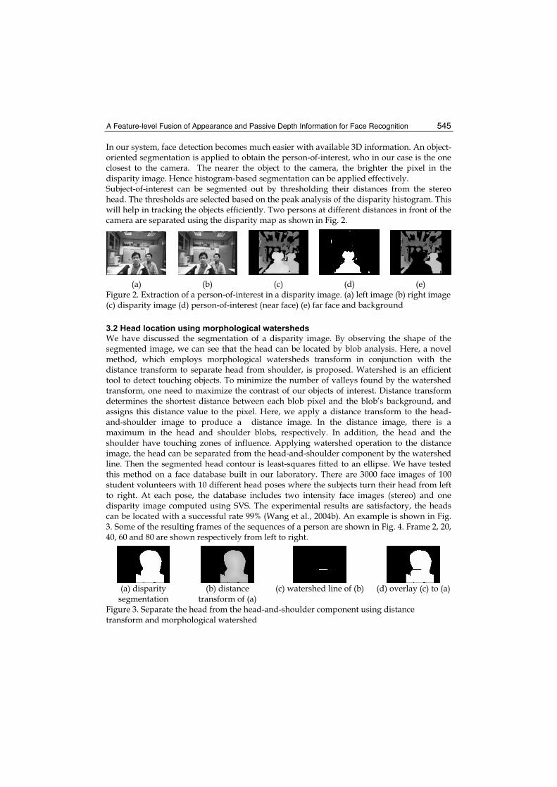
A Feature-level Fusion of Appearance and Passive Depth Information for Face Recognition 545
In our system, face detection becomes much easier with available 3D information. An object-oriented segmentation is applied to obtain the person-of-interest, who in our case is the one closest to the camera. The nearer the object to the camera, the brighter the pixel in the disparity image. Hence histogram-based segmentation can be applied effectively. Subject-of-interest can be segmented out by thresholding their distances from the stereo head. The thresholds are selected based on the peak analysis of the disparity histogram. This will help in tracking the objects efficiently. Two persons at different distances in front of the camera are separated using the disparity map as shown in Fig. 2.
(a) (b) (c) (d) (e) Figure 2. Extraction of a person-of-interest in a disparity image. (a) left image (b) right image (c) disparity image (d) person-of-interest (near face) (e) far face and background
3.2 Head location using morphological watersheds
We have discussed the segmentation of a disparity image. By observing the shape of the segmented image, we can see that the head can be located by blob analysis. Here, a novel method, which employs morphological watersheds transform in conjunction with the distance transform to separate head from shoulder, is proposed. Watershed is an efficient tool to detect touching objects. To minimize the number of valleys found by the watershed transform, one need to maximize the contrast of our objects of interest. Distance transform determines the shortest distance between each blob pixel and the blob’s background, and assigns this distance value to the pixel. Here, we apply a distance transform to the head-and-shoulder image to produce a distance image. In the distance image, there is a maximum in the head and shoulder blobs, respectively. In addition, the head and the shoulder have touching zones of influence. Applying watershed operation to the distance image, the head can be separated from the head-and-shoulder component by the watershed line. Then the segmented head contour is least-squares fitted to an ellipse. We have tested this method on a face database built in our laboratory. There are 3000 face images of 100 student volunteers with 10 different head poses where the subjects turn their head from left to right. At each pose, the database includes two intensity face images (stereo) and one disparity image computed using SVS. The experimental results are satisfactory, the heads can be located with a successful rate 99% (Wang et al., 2004b). An example is shown in Fig. 3. Some of the resulting frames of the sequences of a person are shown in Fig. 4. Frame 2, 20, 40, 60 and 80 are shown respectively from left to right.
(a) disparity segmentation
(b) distance transform of (a)
(c) watershed line of (b) (d) overlay (c) to (a)
Figure 3. Separate the head from the head-and-shoulder component using distance transform and morphological watershed

Face Recognition 546
Figure 4. Head contours of a sequence face images; first row: disparity images; second row: the heads are located by the distance transform and watershed operation; third row: the elliptical head contours. From left to right: frame 2, 20, 40, 60, 80 respectively.
Although the algorithm works well, the watershed line may not incidentally correspond to the neck. Fortunately, this can be detected by checking the eccentricity of the elliptical head. The eccentricity is assumed 1.2 in our experiment. If the watershed is found not to correspond to the neck, i.e. the difference between the ratio of the elliptical head and the assumed one is significant, a candidate head will be placed below the vertically maxima of the silhouette, in a manner similar to (Darrell et al., 2000), and will be refined in the feature tracking stage. (Daniel 2002) proposed a alternative stereo head detection approah. A simple human-torso model is used besides the depth.
3.3 Feature extraction
Many of the existing feature extraction methods are based on artificial template matching. An artificial template is a small rectangular intensity image that contains, for example, an eye corner, where the corner is located in the centre of the template. The image region, which best matches the artificial template is extracted from current image. The problem with artificial template matching is that it fails when it is applied to images that are different from those that were used to generate the artificial image. Recently, the SUSAN (Smallest Univalue Segment Assimilating Nucleus) operator (Smith & Brady, 1997) was found to be an efficient facial feature extraction tool (Hess & Martinez, 2004; Wu et al., 2001; Gu et al., 2001). We adopt the method in our approach where the eye and mouth corners can be located using the SUSAN corner detector. In order to apply the corner detector, we need to establish a rectangular search region for the mouth and two rectangular regions for the left and right eyes respectively. These initial search regions for eye and mouth are found by our method in (Wang & Sung, 1999, 2000). The mouth corners and eye corners were extracted with a reliability of 90% and an average position error of 2.25 pixels. The size of the head is about 50×60 in a 154×114 image. The ground truth of the positions of the eye and mouth corners are found by manually measuring them.

A Feature-level Fusion of Appearance and Passive Depth Information for Face Recognition 547
3.4 Head/Face tracking
(Birchfield, 1998) presented an algorithm for tracking a person’s head. The head’s projection onto the image plane is modeled as an ellipse whose position and size are continually updated by a local search combining the output of a module concentrating on the intensity gradient around the ellipse’s perimeter with that of another module focusing on the color histogram of the ellipse’s interior. Since these two modules have roughly orthogonal failure modes, they serve to complement one another. Extensive experimentation shows the algorithm’s robustness with respect to full 360-degree out-of-plane rotation, up to 90-degree tilting, severe but brief occlusion, arbitrary camera movement, and multiple moving people in the background. We adopted Birchfield’s method to track head/face.
3.5 Pose estimation
As we are using stereo camera, we can compute the pose from the 3D coordinates of the feature points directly, like that by (Matsumoto & Zelinsky, 2000). However, it is found that the pose is quite sensitive to the coordinates’ errors. The head pose can be computed using three feature points, e.g. two eye corners and one mouth corners. Hence, we can get different pose estimations based on different three-point feature groups. We found the result is not stable even if the mean pose of some different poses (e.g. 5 poses can be computed from two eye corners and two mouth corners) is computed. Instead of computing the pose directly based on the 3D coordinates of the feature points, we adopted a robust EM enhanced vanishing point based pose estimetion method (Wang & Sung, 2007) in this chapter. The novel approach assumes the full perspective projection camera model. Our approach employs general prior knowledge of face structure and the corresponding geometrical constraints provided by the location of a certain vanishing point to determine the pose of human faces. To achieve this, eye-lines, formed from the far and near eye corners, and mouth-line of the mouth corners are assumed parallel in 3D space. Then the vanishing point of these parallel lines found by the intersection of the eye-line and mouth-line in the image can be used to infer the 3D orientation and location of the human face. In order to deal with the variance of the facial model parameters, e.g. the ratio between the eye-line and the mouth-line, an EM framework is applied to update the parameters. We first compute the 3D pose using some initially learnt parameters (such as ratio and length) and then adapt the parameters statistically for individual persons and their facial expressions by minimising the residual errors between the projection of the model features points and the actual features on the image. In doing so, we assume every facial feature point can be associated to each of features points in 3D model with some a posteriori probability. The expectation step of the EM algorithm provides an iterative framework for computing the aposterori probabilities using Gaussian mixtures defined over the parameters.
3.6 Normalizations of appearance and disparity images
A face is detected and tracked using stereo vision as the person moves in front of the stereo camera. The frontal face pose is automatically searched and detected from the captured appearance and depth images. These images are subsequently used for face recognition. Using the image coordinates of the two eye centers the image is rotated and scaled to occupy a fixed size array of pixels (88 × 64). In the stereo vision system, the coordinates of pixel are consistent with the coordinates in the left image. The feature points, two eye centers can hence be located in the disparity image. The tip of the nose can be detected in the

Face Recognition 548
disparity image using template matching of (Gordon, 1996). From coplanar stereo vision principle, we have,
d′ = Bf /d (17)
where d′ represents the depth, d is the disparity, B is the baseline and f is the focal length of the calibrated stereo camera. Hence we can compute the depth image from a disparity image with (17). The depth image can be normalized using the depth of the nose tip, i.e. the nose tip of every subject is translated to the same point in 3D relative to the sensor. After that, the depth image is further normalized by the two eye centers. Problems with the 3D data are alleviated to some degree by preprocessing to fill in holes (a region where there is missing 3D data during sensing) and spikes. We adopt the method in (Chang et al., 2004) to detect the spike, and then remove the holes by linear interpolation of missing values from good values around the edges of the hole.
4. Experiments
We evaluate our algorithm on XM2VTS database (Masser et al., 1999) and a large face detabase collected using stereo vision system described in section 3. The purpose is to show the gain in the recognition rate when the depth information is used.
4.1 Experiment on XM2VTS database
The XM2VTS database consists of color frontal, color profile and 3D VRML models of 295 subjects (Masser et al., 1999). The following tests were conducted for performance evaluation. The main reason for adopting this database is that 3D VRML model of those subjects are provided on top of the 2D face images, and this 3D model can be used to generate the depth map for our algorithm.
Figure 5. 3D VRML face models consisting of triangles
Generation of depth images. Depth image is an image where the intensity of a pixel represents the depth of the correspondent point with respect to the 3D VRML model coordinate system. 3D VRML model of a face in XM2VTS database is displayed in Fig 5. There are about 4000 points in a 3D face model to represent the face. The face surface is triangulated with these points. In order to generate a depth image, a virtual camera is placed in front of the 3D VRML model, see Fig. 6. The coordinate system of the camera is defined as follows: the image plane is defined as the X-Y plane and the Z-axis is along the optical axis of the camera and pointing toward the frontal object. The initial plane of Yc-Zc is positioned parallel to Ym-Xm plane of the 3D VRML model. The projective image can be obtained using the perspective transform matrix of the camera. Zc coincides with Zm; however in reverse directions. Xc is parallel to Xm and Yc parallel is to Ym; however they are with reverse directions.
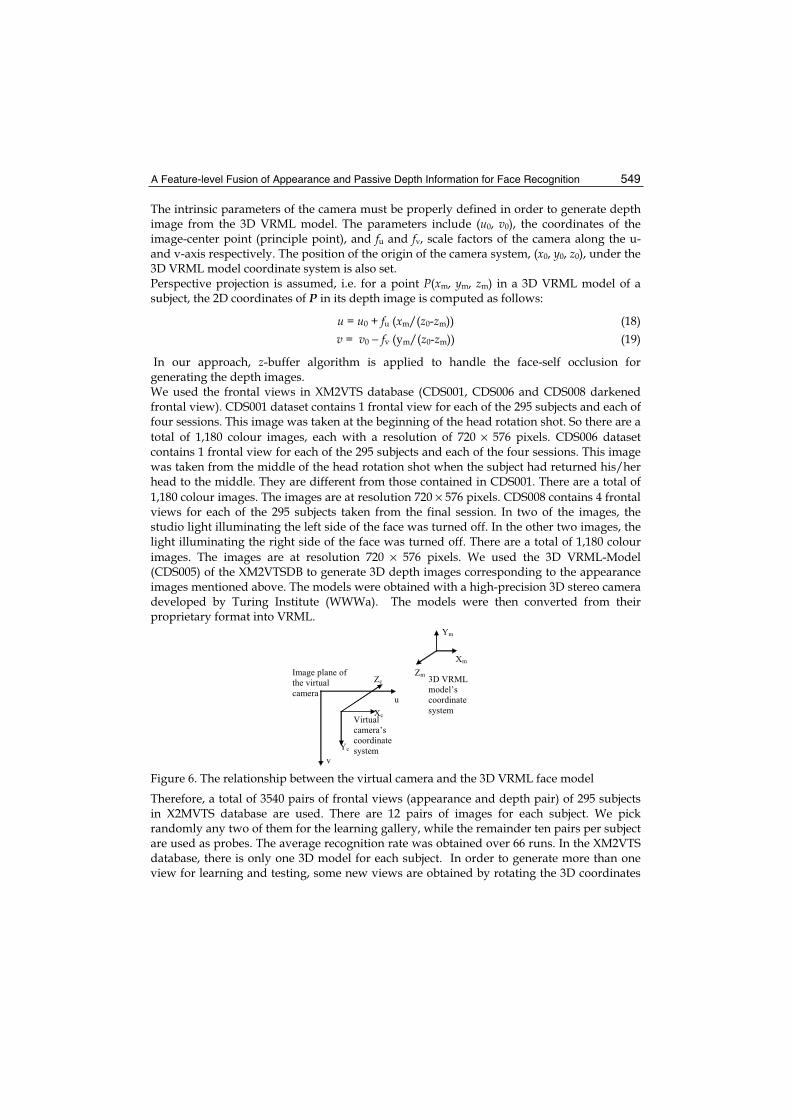
A Feature-level Fusion of Appearance and Passive Depth Information for Face Recognition 549
The intrinsic parameters of the camera must be properly defined in order to generate depth image from the 3D VRML model. The parameters include (u0, v0), the coordinates of the image-center point (principle point), and fu and fv, scale factors of the camera along the u- and v-axis respectively. The position of the origin of the camera system, (x0, y0, z0), under the 3D VRML model coordinate system is also set. Perspective projection is assumed, i.e. for a point P(xm, ym, zm) in a 3D VRML model of a subject, the 2D coordinates of P in its depth image is computed as follows:
u = u0 + fu (xm/(z0-zm)) (18) v = v0 − fv (ym/(z0-zm)) (19)
In our approach, z-buffer algorithm is applied to handle the face-self occlusion for generating the depth images. We used the frontal views in XM2VTS database (CDS001, CDS006 and CDS008 darkened frontal view). CDS001 dataset contains 1 frontal view for each of the 295 subjects and each of four sessions. This image was taken at the beginning of the head rotation shot. So there are a total of 1,180 colour images, each with a resolution of 720 × 576 pixels. CDS006 dataset contains 1 frontal view for each of the 295 subjects and each of the four sessions. This image was taken from the middle of the head rotation shot when the subject had returned his/her head to the middle. They are different from those contained in CDS001. There are a total of 1,180 colour images. The images are at resolution 720 × 576 pixels. CDS008 contains 4 frontal views for each of the 295 subjects taken from the final session. In two of the images, the studio light illuminating the left side of the face was turned off. In the other two images, the light illuminating the right side of the face was turned off. There are a total of 1,180 colour images. The images are at resolution 720 × 576 pixels. We used the 3D VRML-Model (CDS005) of the XM2VTSDB to generate 3D depth images corresponding to the appearance images mentioned above. The models were obtained with a high-precision 3D stereo camera developed by Turing Institute (WWWa). The models were then converted from their proprietary format into VRML.
Xm
Ym
Zm
Xc
Yc
Zc
u
v
3D VRML
model’s
coordinate
system Virtual
camera’s
coordinate
system
Image plane of
the virtual
camera
Figure 6. The relationship between the virtual camera and the 3D VRML face model
Therefore, a total of 3540 pairs of frontal views (appearance and depth pair) of 295 subjects in X2MVTS database are used. There are 12 pairs of images for each subject. We pick randomly any two of them for the learning gallery, while the remainder ten pairs per subject are used as probes. The average recognition rate was obtained over 66 runs. In the XM2VTS database, there is only one 3D model for each subject. In order to generate more than one view for learning and testing, some new views are obtained by rotating the 3D coordinates

Face Recognition 550
of VRML model away the frontal (about the Ym axes) by some degrees. In our experiments, the new views obtained at ±1°, ±3°, ±5°, ±7°,±9°,±11°.Some of the normalized face image samples in XM2VTS database are shown in Fig. 7, where appearance face images are shown in Fig. 7(a) and the correspondent depth images are shown in Fig. 7(b). The resolution of the images is 88 × 64. We can see significant changes in illumination, expressions, hair, and eye glasses/no eyeglasses due to longer time lapse (four months) in photograph taking. The first 40 Eigenfaces of 2D and 3D training samples are shown in Fig. 8.
(a) Normalized appearance face images, the column 1-4: images in CDS001; column 5-8: images in CDS006; column 9-12: images in CDS008
(b) Normalized depth images corresponding to (a) Figure 7. Some normalized samples (appearance and corresponding depth images) from XM2VTS database
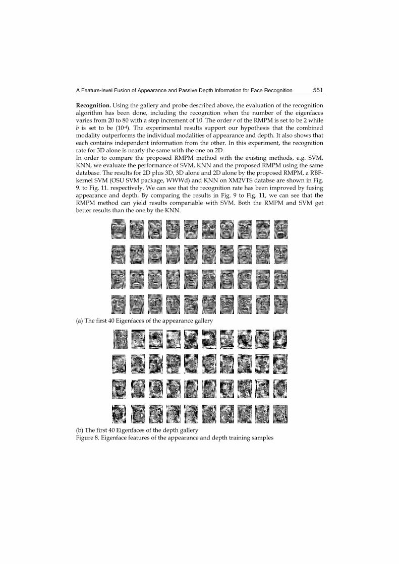
A Feature-level Fusion of Appearance and Passive Depth Information for Face Recognition 551
Recognition. Using the gallery and probe described above, the evaluation of the recognition algorithm has been done, including the recognition when the number of the eigenfaces varies from 20 to 80 with a step increment of 10. The order r of the RMPM is set to be 2 while b is set to be (10-4). The experimental results support our hypothesis that the combined modality outperforms the individual modalities of appearance and depth. It also shows that each contains independent information from the other. In this experiment, the recognition rate for 3D alone is nearly the same with the one on 2D. In order to compare the proposed RMPM method with the existing methods, e.g. SVM, KNN, we evaluate the performance of SVM, KNN and the proposed RMPM using the same database. The results for 2D plus 3D, 3D alone and 2D alone by the proposed RMPM, a RBF-kernel SVM (OSU SVM package, WWWd) and KNN on XM2VTS databse are shown in Fig. 9. to Fig. 11. respectively. We can see that the recognition rate has been improved by fusing appearance and depth. By comparing the results in Fig. 9 to Fig. 11, we can see that the RMPM method can yield results compariable with SVM. Both the RMPM and SVM get better results than the one by the KNN.
(a) The first 40 Eigenfaces of the appearance gallery
(b) The first 40 Eigenfaces of the depth gallery Figure 8. Eigenface features of the appearance and depth training samples

Face Recognition 552
4.2 Experiment on stereo vision system
Encouraged by the good performance of the recognition algorithm on XM2VTS database, we implemented the algorithms on a stereo vision system. We aim at identifying a face by fusing disparity/depth and intensity information from a binocular stereo vision system (WWWb), which outputs the disparity/range information automatically in real-time. The existing 3D face recognition techniques assume the use of active 3D measurement for 3D face image capture. However, active methods employ structured illumination (structure projection, phase shift, etc) or laser scanning, which is not desirable in many applications. In this paper, we use passive stereo to obtain 3D face images and a face recognition using appearance and depth is presented. A major problem of using passive stereo is its low accuracy, and thus no passive method for 3D face recognition has been reported. Thanks to the technical progress in 3D capture/computing, an affordable real-time stereo system is now available by which one can get a comparable resolution of 3D data in real-time. In this paper, we used SRI stereo head (WWWb), in which the stereo process interpolates disparities to 1/16 pixels. Both internal and external parameters are calibrated by an automatic calibration procedure. The disparity change, Δd is (1/16)×7.5 μm = 0.46875 μm. Here a pixel size of 7.5 μm. We used MAGA-D stereo head, where the baseline, B, is 9cm, the focus length, f, is 16mm, Hence, when the distance from the subject to the stereo head, s,is 1m, the range resolution, i.e. the smallest change in range that is discernable by the stereo geometry,
Δr = (s2/Bf)Δd = (1m2/(90mm×16mm))×0.46875μm×10-3 = 0.3255 mm
The range resolution is high enough for our face recognition applications, a fact verified by our experiments. The SRI Small Vision System outputs the disparity/range information automatically in real-time. The size of the left image, right image and disparity image is 320 × 240. In our experiments, the distance between the person-of-interest to the camera is about 1m to 1.5m. At this distance, the size of the face region is big enough and the disparity image is good with 16 mm lens. We calibrate the camera within this distance range in order that a good disparity image can be obtained as the distance between the person to the camera is within the distance range. In our experiments, the entire face detection, tracking, feature extraction, pose estimation and recognition can be performed in real time at 15 frames per second on a P4 3.46Ghz, 1G memory PC. When a subject is found to be a new user by the system, i.e. when the output of the reduced model is less than 0.5, the user will be registered by the system automatically. Using the above-mentioned system, a database is built to include 116 subjects. There are 12 pairs of images (appearance and depth) for each subject. The face images are captured over a period of six months. Some normalized appearance and disparity images are shown in Fig. 12. We pick randomly any two of them for the learning gallery, while the remainder ten pairs per subject are used as probes. The average recognition rate was obtained over 66 runs. We use the same parameters for RMPM on XM2VTS database, i.e. the order of the RMPM, r, is set to be 2. b is set to be (10-4). The new users that are not included in the database can be registered automatically using the method described in Section 2.4. The recognition results for 2D plus 3D, 3D alone and 2D alone by using the proposed RMPM, SVM and KNN are given in Fig. 13 to Fig. 15 respectively. We can see that the RMPM method can yield results comparable with SVM.
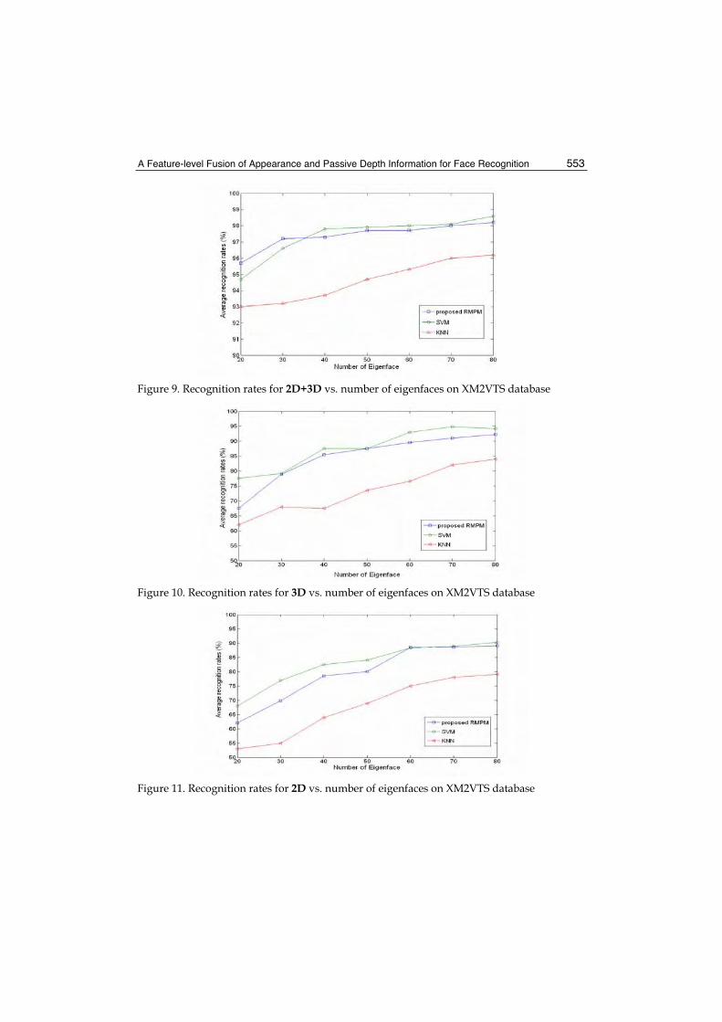
A Feature-level Fusion of Appearance and Passive Depth Information for Face Recognition 553
Figure 9. Recognition rates for 2D+3D vs. number of eigenfaces on XM2VTS database
Figure 10. Recognition rates for 3D vs. number of eigenfaces on XM2VTS database
Figure 11. Recognition rates for 2D vs. number of eigenfaces on XM2VTS database

Face Recognition 554
5. Conclusion
In this paper, we contributed a stereo face recognition formulation which combines appearance and disparity/depth at feature level. We showed that the present-day passive stereovision in combination with 2D appearance images can match up to other methods which rely on active depth data. A Reduced Multivariate Polynomial Model was adopted to fuse the appearance and disparity images. RMPM is extended so that the problem of new-user registration can be overcome. We evaluated the performance of such fusion on XM2VTS face database. The evaluation results, which included results from appearance alone, depth alone and fusion of them respectively, using XM2VTS database, showed improvement of recognition rate from combining 3D information and 2D information. The performance using fused depth and appearance was found to be the best among the three tests. Furthermore, we implemented the algorithm on a real-time stereo vision system where near-frontal views were selected from stereo sequence for recognition. The evaluation results, which included results from appearance alone, depth alone and fusion of them respectively, using a database collected by the stereo vision system also showed improvement of the recognition rate by combining 3D information and 2D information. The RMPM can yield comparable results with SVM while the computation load of the RMPM is much lower than SVM.
Figure 12. Normalized appearance and disparity images from the stereo vision system
The face recognition approach is anticipated to be useful for some on-line applications, such as visitor identification, ATM, and HCI. Prior to such implementations in physical systems, the performance of the system should be investigated on data with larger pose variance in terms of the verification accuracy. This is our future work. In addition, new dimension reduction method could be investigated in the future work.

A Feature-level Fusion of Appearance and Passive Depth Information for Face Recognition 555
Figure 13. Recognition rates for 2D+3D vs. number of eigenfaces on our database
Figure 14. Recognition rates for 3D vs. number of eigenfaces on our database
Figure 15. Recognition rates for 2D vs. number of eigenfaces on our database

Face Recognition 556
6. References
Beumier C. & Acheroy M. (1998). Automatic face verification from 3D surface, Proceedings of British Machine Vision Conference, pp. 449-458.
Beumier C. & Acheroy M. (2001). Face verification from 3D and grey level clues, Pattern Recognition Letters, Vol. 22, 1321-1329.
Birchfield, S. (1998). An elliptical head tracking using intensity gradients and color histograms, Proceedings IEEE International Conference on Computer Vision and Pattern Recognition, Santa Barbara, California, pp. 232-237.
Blanz V. & Vetter T. (1999). A Morphable Model for the Synthesis of 3D Faces, Proceedings of SIGGRAPH, pp. 187-194.
Blanz V. & Vetter T. (2003). Face Recognition Based on Fitting a 3D Morphable Model, IEEE Transactions on Pattern Analysis and Machine Intelligence, Vol. 25, No. 9, 1063-1074.
Bowyer K. W.; Chang K. & P. Flynn (2006). A survey of approaches and challenges in 3D and multimodal 3D + 2D face recognition, Computer Vision and Image Understanding,Vol. 101, 1-15.
Bruneli R. & Falavingna D. (1995). Person identification using multiple cues, IEEE Transactions on Pattern Analysis and Machine Intelligence, Vol. 17, No. 10, 955-966.
Chang K.; Bowyer K.; Flynn P. (2003). Face Recognition Using 2D and 3D Facial Data, IEEE International Workshop on Analysis and Modeling of Faces and Gestures, Nice, France, pp. 187-194.
Chang K.; Bowyer K. & Flynn P., (2004). Multi-biometrics using facial appearance, shape and temperature, Proceedings of IEEE International Conference on Automatic Face and Gesture Recognition, pp. 43-48.
Chang K.; Bowyer K. & Flynn P. (2005). An Evaluation of Multimodal 2D+3D Face Biometrics, IEEE Transactions on Pattern Analysis and Machine Intelligence, Vol. 27, No. 4, 619-624.
Chellappa R.; Wilson C.L. & Sirohey S. (1995). Human and machine recognition of faces, Proceedings of the IEEE, Vol. 83, No. 5, 705-740.
Choudhury T.; Clarkson B.; Jebara T. & Pentland A. (1999). Multimodal person recognition using unconstrained audio and video, Proceedings International Conference on Audio and Video Based Person Authentication, pp.176-181.
Chua C. S.; Han F. & Ho Y. K. (2000). 3D face recognition using point signature, Proceedings of IEEE International Conference on Automatic Face and Gesture Recognition, pp. 233-238.
Daniel B. R. & Martin H. (2002).Head Tracking Using Stereo Machine Vision and Applications, Vol. 13, 164–173
Darrell T.; Gordon G.; Harville M. & Woodell J. (2000). Integrated person tracking using stereo, color and pattern detection, International Journal of Computer Vision, Vol. 37, No. 2, 175-185.
Gordon G. (1996). Face Recognition Based on Depth Maps and Surface Curvature, Proceedings of IEEE International Conference on Automatic Face and Gesture Recognition, pp.176-181.
Gu H.; Su G. & Du C. (2001). Feature points extraction from face, Proceedings of Conference on Image and Vision Computing, pp. 154-158.

A Feature-level Fusion of Appearance and Passive Depth Information for Face Recognition 557
Hess M. & Martinez M. (2004). Facial feature extraction based on the smallest univalue segment assimilating nucles (susan) algorithm, Proceedings of Picture Coding Symposium, San Franscisco, California.
Hong L. & Jain A.(1998). Integrating faces and fingerprints for person identification, IEEE Trans. on Pattern Analysis and Machine Intelligence, Vol. 20, No. 12, 1295–1307.
Kittler J.; Hatef M.; Duin R. P.W. & Matas J. (1998). On combining classifiers, IEEE Trans. on Pattern Analysis and Machine Intelligence, Vol. 20, No. 3, 226-239.
Lee J. C. & Milios E. (1990). Matching range Images of human faces, Proceedings of. IEEE International Conference on Computer Vision, pp. 722-726.
Lu X. & Jain A. K. (2005). Deformable analysis for 3D face matching, Proceedings of 7th IEEE Workshop on Applications of Computer Vision, pp. 99-104.
Masser K.; Matas J.; Kittler J.; Luettin J. & Maitre G. (1999). XM2VTSDB: The extended M2VTS Database, Proceedings of AVBPA, pp. 72-77.
Matsumoto Y. & Zelinsky A. (2000). An algorithm for real-time stereo vision implementation of head pose and gaze direction measurement. Proceedings IEEE International Conference on Automatic Face and Gesture Recognition, pp.499-505.
Morency L.-P.; Rahimi A.; Checka N. & Darrell T. (2002). Fast Stereo-Based Head Tracking for Interactive Environments, Proceedings of IEEE International Conference on Automatic Face and Gesture Recognition, pp. 375-380.
Neter J.; Kutner M. H.; Nachtsheim C. J. & Wasserman W. (1996). Applied Linear Regression Models, third ed.
Pan G.; Wu Y. & Wu Z. (2003). Investigating profile extraction from range data for 3D recognition, Proceedings of IEEE International Conference on Systems, Man and Cybernetics, pp. 1396-1399.
Rafael M.-S.; Eugenio A.; Miguel G.-S. & Antonio G. (2005). People detection and tracking through stereo vision for human-robot interaction. Proceedings of the Mexican International Conference on Artificial Intelligence, Lectures Notes on Artificial Intelligence 3789, Ed. Springer, pp. 337-346.
Smith S. M. & Brady J. M. (1997). SUSAN-A new approach to low level image processing, International Journal of Computer Vision, Vol. 23, 45-78.
Socolinsky D.A.; Selinger A. & Neuheisel J.D. (2003). Face recognition with visible and thermal infrared imagery, Computer Vision and Image Understanding, Volumn 91, Issue 1-2, 72 – 114.
Taylor S. & Cristianini N. (2004). Kernel methods for pattern analysis, Cambridge University Press.
Toh K.-A. ; Tran Q.-L. & Srinivasan D. (2004). Benchmarking a reduced multivariate polynomial pattern classifier, IEEE Transactions on PAMI, Vol. 26, No. 6, 740-755.
Tran Q.-L.; Toh K.-A. & Srinivasan D. (2004). Adaptation to changes in multimodal biometric authentication, Proceedings of the 2004 IEEE Conference on Cybernetics and Intelligent Systems, pp.981-985.
Tsalakanidou F.; Tzovaras D. & StrintzisAfzal M. G. (2003). Use of depth and colour eigenfaces for face recognition, Pattern Recognition Letters, Volume 24, Issues 9-10, 1427-1435
Wang J.-G. & Sung E. (1999). Frontal-view face detection and facial feature extraction using color and morphological operations, Pattern Recognition Letters, Vol. 20, 1053-1068.

Face Recognition 558
Wang J.-G. & Sung E. (2000). Morphology-based front-view facial contour detection, In: Proceedings of IEEE International Conference on Systems, Man and Cybernetics,Nashville, Tennessee, USA, 8-11 October 2000.
Wang J.-G. ; Kong H. & Venkateswarlu R. (2004a). Improving face recognition rates by combining color and depth Fisherfaces,″ Proceedings of 6th Asian Conference on Computer Vision, pp.126-131.
Wang J.-G.; Lim E. T. & Venkateswarlu R. (2004b). Stereo face detection/tracking and recognition, Proceedings of IEEE International Conference on Image Processing, pp. 638-644.
Wang J.-G.; Toh K.-A. & Venkateswarlu R. (2005). Fusion of appearance and depth information for face recognition, Proceedings of 5th International Conference on Audio- and Video–Based Biometric Person Authentication, pp. 919-928.
Wang J.-G.; Kong H. & Yau W.-Y. (2006). Bilateral Two Dimensional Linear Discriminant Analysis for Stereo Face Recognition. Proceedings of IEEE International Conference on Pattern Recognition, pp.429-432
Wang J.-G.; Sung E. (2007). EM Enhancement of 3D Head Pose Estimated by Point at Infinity, Image and Vision Computing, Special issue of HCI'04 Workshop on Computer Vision in Human-Computer Interaction, Lew Michael S. et al. (eds), to appear.
Wu H.; Inada J.; Shioyama T.; Chen Q. & Simada T. (2001). Automatic Facial Feature Points Detection with SUSAN Operator, Proceedings of Scandinavian Conference on Image Analysis, pp. 257-263.
WWWa. Turing Institute: http://www.turing.gla.ac.ukWWWb. Videre Design, MEGA-D Megapixel Digital Stereo Head,
http://users.rcn.com/mclaughl.dnai/sthmdcs.htm WWWc. The Face Recognition Grand Challenge, http://www.frvt.org/FRGC/ WWWd. OSU SVM package, http://svm.sourceforge.net/download.shtml Yacoob Y. & Davis L. S. (1994). Labeling of human faces components from range data,
CVGIP: Image Understanding, Vol. 60, No. 2, 168-178. Zhao W.; Chellappa R.; Rosenfeld A. & Phillips P. J. (2003). Face Recognition: A Literature
Survey, ACM Computing Surveys, 399-458.


