112
Facility Location and Network Design With Congestion Costs and Interdependency Gilberto de Miranda Junior 05/25/2004

Facility Location and Network Design
With Congestion Costs and
Interdependency
Gilberto de Miranda Junior
05/25/2004


To my parents, my wife and my daughter.


Abstract
In this work we develop mathematical programming formulations for locationmodels, congested network design models and the integration of both. Locationand network design problems arise in several applications of Computer Sci-ence, Engineering and Economy. Nowadays, these problems can not be solvedefficiently, what is our major motivation. Established the relevance of theseproblems, we try to expand their solution frontiers, rewriting them with theaid of flow formulations and using a Benders decomposition framework. Ourmain goal is to deal with large scale mixed integer programming problems as theQuadratic Assignment Problem, the Uncapacitated Hub Location Problem andlarge scale mixed integer nonlinear programming problems. Extensive computa-tional experiments were carried out. The output data is analyzed and discussed,becoming possible to evaluate the quality of the proposed approach
v


Contents
Abstract v
1 Problem Context and Motivation 1
1.1 The Location of Economic Activities . . . . . . . . . . . . . . . . 11.2 The Local Access Network Design . . . . . . . . . . . . . . . . . 21.3 Facility Location and Network Design . . . . . . . . . . . . . . . 3
2 Assignment Problems 5
2.1 Theory and Background . . . . . . . . . . . . . . . . . . . . . . . 52.2 The Linear Assignment Problem . . . . . . . . . . . . . . . . . . 72.3 The Quadratic Assignment Problem . . . . . . . . . . . . . . . . 8
2.3.1 Alternative Problem Formulations, Linearizations and Bounds 92.3.2 Flow Formulations for QAP . . . . . . . . . . . . . . . . . 112.3.3 A Brief Computational Experiment . . . . . . . . . . . . . 12
2.4 Benders Decomposition of the Problem . . . . . . . . . . . . . . . 162.4.1 Subproblems . . . . . . . . . . . . . . . . . . . . . . . . . 232.4.2 Enhancing the Benders Decomposition Algorithm with
Flow Equilibrium Constraints . . . . . . . . . . . . . . . . 242.5 Computational Experiments Using Enhanced Benders Decompo-
sition . . . . . . . . . . . . . . . . . . . . . . . . . . . . . . . . . . 262.6 Concluding Remarks . . . . . . . . . . . . . . . . . . . . . . . . . 28
3 The Placement of Electronics with Thermal Effects 33
3.1 Introduction . . . . . . . . . . . . . . . . . . . . . . . . . . . . . . 333.2 Thermal Modeling and Temperature Penalty Costs . . . . . . . . 34
3.2.1 Maximum Temperature and Penalty Costs . . . . . . . . 353.3 Computational Experiments . . . . . . . . . . . . . . . . . . . . . 38
3.3.1 Experiment Description . . . . . . . . . . . . . . . . . . . 383.3.2 Numerical Results . . . . . . . . . . . . . . . . . . . . . . 41
3.4 Concluding Remarks . . . . . . . . . . . . . . . . . . . . . . . . . 42
4 The Local Access Network Design With Congestion Costs 47
4.1 Introduction . . . . . . . . . . . . . . . . . . . . . . . . . . . . . . 474.2 Multi-commodity Flow Formulation . . . . . . . . . . . . . . . . 49
vii

4.2.1 Variables and Parameters . . . . . . . . . . . . . . . . . . 504.2.2 Mixed Integer Nonlinear Program . . . . . . . . . . . . . 504.2.3 Theoretical Properties of the Linear and the Concave Ver-
sions . . . . . . . . . . . . . . . . . . . . . . . . . . . . . . 514.2.4 Convexification of Leasing and Congestion Costs . . . . . 52
4.3 Benders Decomposition of the Problem . . . . . . . . . . . . . . . 534.3.1 Problem Manipulations . . . . . . . . . . . . . . . . . . . 534.3.2 Subproblems . . . . . . . . . . . . . . . . . . . . . . . . . 564.3.3 Master Problem . . . . . . . . . . . . . . . . . . . . . . . 594.3.4 Algorithm . . . . . . . . . . . . . . . . . . . . . . . . . . . 604.3.5 Avoiding Cycles . . . . . . . . . . . . . . . . . . . . . . . 61
4.4 Computational Results . . . . . . . . . . . . . . . . . . . . . . . . 624.5 Conclusions . . . . . . . . . . . . . . . . . . . . . . . . . . . . . . 66
5 Integrating Facility Location and Network Design 69
5.1 Problem Description . . . . . . . . . . . . . . . . . . . . . . . . . 695.2 Mathematical Programming Formulations . . . . . . . . . . . . . 71
5.2.1 Improving the Design of the Local Access Network . . . . 745.2.2 Generalized Model Including Hub Transshipment and Net-
work Design . . . . . . . . . . . . . . . . . . . . . . . . . . 775.3 Computational Experiences . . . . . . . . . . . . . . . . . . . . . 78
5.3.1 Benders Decomposition for the p-Hub Median Problemand the Uncapacitated Hub Location Problem . . . . . . 78
5.3.2 The Integrated Model: QAP + Local Access NetworkDesign With Congestion Costs . . . . . . . . . . . . . . . 81
5.3.3 Testing the Hub Transshipment Network Design Model . 815.4 Concluding Remarks . . . . . . . . . . . . . . . . . . . . . . . . . 82
6 Conclusions and Future Work 87
6.1 Contributions . . . . . . . . . . . . . . . . . . . . . . . . . . . . . 876.1.1 The Quadratic Assignment Problem . . . . . . . . . . . . 876.1.2 The Placement of Electronics With Thermal Effects . . . 886.1.3 The Local Access Network Design With Congestion Costs 886.1.4 Integrating Facility Location and Network Design . . . . . 88
6.2 Hints for Future Work . . . . . . . . . . . . . . . . . . . . . . . . 89

List of Figures
2.1 Different representations of assignments. . . . . . . . . . . . . . . 52.2 Perfect matching in a bipartite graph and corresponding network
flow model. . . . . . . . . . . . . . . . . . . . . . . . . . . . . . . 62.3 Comparison of linear programming bounds for both formulations. 172.4 Comparison of lp computing times for both formulations. . . . . 182.5 Comparison of mip computing times for both formulations. . . . 192.6 Comparison of mip computing times for both formulations. . . . 202.7 Comparison of mip computing times for both formulations. . . . 212.8 Comparison of mip computing times for both formulations. . . . 222.9 An example of automatic construction of a feasible solution for
the dual subproblem. . . . . . . . . . . . . . . . . . . . . . . . . . 232.10 Evolution of computing times with p/q ratio. . . . . . . . . . . . 292.11 Evolution of computing times with p/q ratio. . . . . . . . . . . . 302.12 Evolution of computing times with p/q ratio. . . . . . . . . . . . 31
3.1 QAP instance and Finite Volume Grid representation. . . . . . . 363.2 The penalty overheating cost function, for a threshold tempera-
ture of 85 Celsius. . . . . . . . . . . . . . . . . . . . . . . . . . . 373.3 Evolution of bounds during the method execution. . . . . . . . . 393.4 Number of Benders iterations versus p/q cost reason. . . . . . . . 443.5 Execution time [s] versus p/q cost reason. . . . . . . . . . . . . . 443.6 Temperature field for ste36a placement solution without over-
heating penalty. . . . . . . . . . . . . . . . . . . . . . . . . . . . . 453.7 Temperature field for ste36a placement solution considering over-
heating penalty. . . . . . . . . . . . . . . . . . . . . . . . . . . . . 45
4.1 The tree network design problem. . . . . . . . . . . . . . . . . . . 484.2 An example of convexified integrated leasing and congestion cost
function. . . . . . . . . . . . . . . . . . . . . . . . . . . . . . . . . 54
5.1 Hub-and-spoke system with different kinds of local access networks. 705.2 Possible routes for the commodity ij for a given x = xh. . . . . . 735.3 A city partitioned in regions . . . . . . . . . . . . . . . . . . . . . 845.4 A feasible solution . . . . . . . . . . . . . . . . . . . . . . . . . . 85
ix


List of Tables
2.1 Linear programming bounds for both formulations under com-parison and respective computing times. . . . . . . . . . . . . . . 13
2.2 Problem dimensions for test instances, number of integer andcontinuous variables, p/q ratio and a comparison of integer mixedprogramming computing times. . . . . . . . . . . . . . . . . . . . 14
2.3 Problem dimensions for test instances, number of integer andcontinuous variables, p/q ratio and a comparison of mixed integerprogramming computing times. . . . . . . . . . . . . . . . . . . . 15
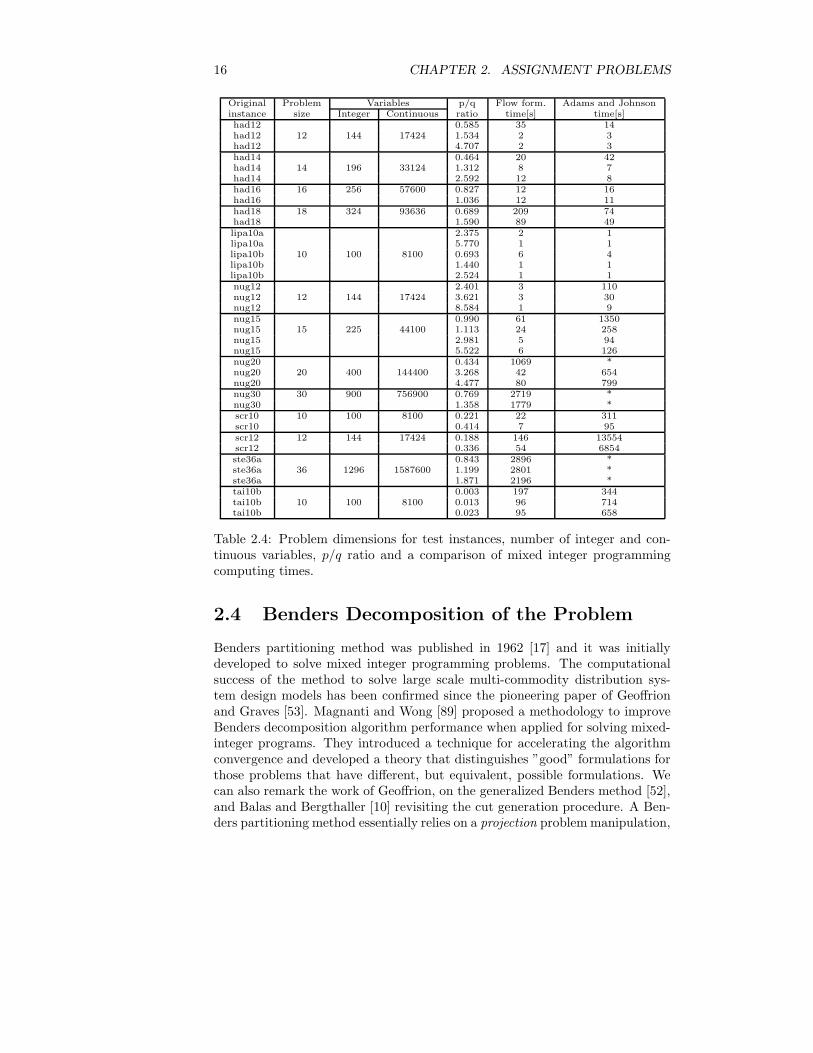
2.4 Problem dimensions for test instances, number of integer andcontinuous variables, p/q ratio and a comparison of mixed integerprogramming computing times. . . . . . . . . . . . . . . . . . . . 16
2.5 Problem dimensions for test instances, number of integer andcontinuous variables, p/q ratio and computing times for Bendersdecomposition. . . . . . . . . . . . . . . . . . . . . . . . . . . . . 26
2.6 Problem dimensions for test instances, number of integer andcontinuous variables, p/q ratio and computing times for Bendersdecomposition. . . . . . . . . . . . . . . . . . . . . . . . . . . . . 27
2.7 Problem dimensions for test instances, number of integer andcontinuous variables, p/q ratio and computing times for Bendersdecomposition and flow formulation. . . . . . . . . . . . . . . . . 28
2.8 Evolution of computing times for Benders algorithm and the flowformulation . . . . . . . . . . . . . . . . . . . . . . . . . . . . . . 30
2.9 Evolution of computing times for Benders algorithm and the flowformulation . . . . . . . . . . . . . . . . . . . . . . . . . . . . . . 31
2.10 Solution of larger instances using the Benders algorithm. . . . . . 32
3.1 Thermo-physical properties for the thermal model. . . . . . . . . 363.2 Test instances for computational experiments. . . . . . . . . . . . 403.3 Results for computational experiments - first set. . . . . . . . . . 413.4 Results for computational experiments - second set. . . . . . . . 423.5 Results for computational experiments - third set. . . . . . . . . 43
4.1 Network Dimensions for Test Problems. . . . . . . . . . . . . . . 634.2 Average computing time, number of Benders iterations and num-
ber of cycle avoiding constraints for experiments 1 to 5. . . . . . 65
xi

4.3 Average computing time, number of Benders iterations, Nonlin-ear/linear gap and number of different arcs for experiments 1 to5. . . . . . . . . . . . . . . . . . . . . . . . . . . . . . . . . . . . . 66
4.4 Computing time, number of Benders iterations, number of cycleavoiding constraints for experiment 6. . . . . . . . . . . . . . . . 67
4.5 Computing time, number of Benders iterations, and Nonlinear/lineargap for experiment 6. . . . . . . . . . . . . . . . . . . . . . . . . . 68
5.1 Benders decomposition for the p-Hub Median Problem. . . . . . 795.2 Benders decomposition for the Uncapacitated Hub Location Prob-
lem. . . . . . . . . . . . . . . . . . . . . . . . . . . . . . . . . . . 805.3 Computational results for the integrated model. . . . . . . . . . . 815.4 Report for a brief experiment using the Hub Transshipment Net-
work Design model. . . . . . . . . . . . . . . . . . . . . . . . . . . 82

Chapter 1
Problem Context and
Motivation
1.1 The Location of Economic Activities
There are important areas of economic analysis in which progress depends ofmethods for solving or analyzing problems for efficient allocation of indivisibleresources. There are practical decision problems that we can cite. For instance,to determine suitable numbers of machine tools of various kinds within a plant,or to define the number of channel capacities and frequencies in telecommuni-cation networks.
Furthermore, indivisibilities in the more highly specialized human or ma-terial factors of production are always at the root of increasing returns to thescale of production. They can arise within the plant or firm, or in relation witha cluster of firms. Strong interest in the effects of indivisibilities comes from thefact that: if industry increasing returns to scale persist at a production levelthat sizes the total demand in the respective market, we do not have perfectcompetition and the efficiency of a price system in allocating resources is re-duced. Summarizing, the location theory of economic activities is dependent onthe indivisibilities of human and material resources to better explain the reality.This was preconceived by Koopmans and Beckmann [77]. These indivisibilities,by the way, are responsible for some of the greatest mathematical challengesthat Mathematical Programming and Computer Science have been facing in thelatest 45 years.
It is possible to describe a huge list of practical applications of locationproblems. Among them, the best location of producers in a multi-commoditytransportation network, the best location of warehouses and plants, given thelocation of his customers and suppliers, the best location of points of inflowor outflow in transportation networks. On the highly competitive economicsystem created by globalization, it is unnecessary to point out that every singlecost component is important: in one side the minimization of production (fixed
1

2 CHAPTER 1. PROBLEM CONTEXT AND MOTIVATION
or operational)costs improves any organization survivability, at the other sideimproves the quality of the provided services, maximizing social benefits.
All the systems that have ”hub-and-spoke” features are candidates to loca-tional studies. In a major scale, we can think about the location of private andpublic facilities to improve the quality of service, and thus quality of life, for agiven population. In this context, the facility that we are talking about can begenerally called a server, an indivisible resource that is responsible for locallyprovide access to some kind of commodity for final customers and which is con-nected with other facilities by a transportation network. The commodity beingtransported from and to these servers can be water, fuel and other petroleumsub-products, electrical energy in power transmission networks, data and othersignals in telecommunication and computer networks. The servers can be merelyconcentrators or complex base stations, depending on the commodity and thetransportation technology associated.
Several researchers are dealing with location problems. The work and re-search conducted around Assignment Problems, which are some of the simplestapproaches to give answers to location theorists, is intensively increasing. Thework of Koopmans and Beckmann[77] is a landmark for location theory. Forsome traditional surveys on this subject, we suggest the work of Motzkin [99],Losch [82], Kuhn [79], Mills [98], Samuelson [121] and Heffley [61]. On the lastyears, deserve attention the work of Beasley [14], Christofides and Beasley [36],Franca and Luna [45], Mateus and Luna [92], Aikens [2] and Mateus and Thizy[94]. Assignment problems are being studied more recently by Burkard [23],Balas and Saltzman[11], Burkard and Cela [27], Burkard, Cela, Pardalos andPitsoulis [28], Cela [26], Anstreicher [4], Anstreicher and Brixius [5], Anstreicher,Brixius, Goux and Linderoth [6].
1.2 The Local Access Network Design
Once defined the location of the servers, the question on how to design the localaccess network, that the final customer will use to access a server, naturallyarises. The quality of the local access network, in some cases, is representativeof a great amount of the total cost. Network design problems have found wideapplication in computer networks and telecommunication systems, exploring is-sues of topological design, routing and capacity assignment [21, 47, 93]. Thehierarchical organization of telephone and computer networks plays a majorrole, inasmuch as optimized levels of customers concentration enables substan-tial economies of scale of increasing transmission bandwidth. Cost minimizationis the objective of most of these operations research models, the main differenceamong the models being the hierarchical level of network design, typically con-cerning backbones or local access networks. In this work we have consideredthe local access network design problem with congestion costs. The local accessnetwork design problem consists of linking a supply node to its demand nodessatisfying their demand at minimal total cost. The problem presents heteroge-neous terminals, and there are also Steiner or transshipment nodes. Each arc

1.3. FACILITY LOCATION AND NETWORK DESIGN 3
of the network has three associated costs: a linear variable operational cost de-pending on the flow through the arc, a fixed cost associated with the installationof the arc and a non-linear congestion cost that penalize flows close to implicitcapacities. This problem can be viewed as a generalization of the Steiner treeproblem on a directed graph [85]. In fact, if we neglect variable and congestioncosts at the arcs we will have basically the Steiner problem, and in this sensewe are treating a NP-Hard problem, for which some computational strategieshave been devised [87, 128, 75, 83, 67, 68]. On the other hand, if we neglectfixed and congestion costs on the arcs we have the single source transshipmentproblem, which can be solved easily [40].
As one can see, it is possible to use this approach to deal with any kind ofnetwork flow problem that has a single source tree as optimal solution. Thenetwork design problem associated with centralized computer networks and themultiparty multicast tree construction problem are good examples. The last onehas been treated with the aid of heuristics [69], but on the two versions pointedby the literature, the Single Source Tree Networks - where we have a true rootof the multi-party multicasting tree - and the Core Based Tree Networks - wherea single node, the core, is chosen to play a role as the tree root - it is possibleto adjust the data to make the model treatment to accomplish the nature ofthe problem. The provision of multi-point connections is one of most importantservices that will be required in future broadband communication networks thatsupport distributed multimedia applications. Multimedia video-conference ap-plications, for instance, require that audio and video be transmitted to multipleconference participants simultaneously. This requires that an efficient multi-cast capability be provided by the underlying network. Beyond problems intelecommunications and centralized computer networks, this approach is usefulto deal also with petrochemical products distribution networks, water distri-bution networks, and many other local access networks (distributing energy,material resources or signals and data) under mild assumptions.
1.3 Facility Location and Network Design
Network location models have been used extensively to analyze and determinethe location of facilities. Classical network models include the location set cov-ering problem [124], the maximum covering location problem [37] and p-medianand p-center problems [60].
In addition to these, the uncapacitated facility location problem[78] has beentreated in its own right and is also known as simple plant location problem andwarehouse location problem. All these models locate facilities on a given network.However, the topology of the underlying network may have profound impact onfacility location. Models that integrates the tasks of facility location and networkdesign has being presented by Melkote and Daskin [97], [96], Berger et. al. [18],Berman, Ingco and Odoni [19] and Campbell [34]. In this kind of problems, a setof nodes is given that represents the demand nodes, as well as candidate facilitylocations, and a set of uncapacitated links. Each link has a fixed construction

4 CHAPTER 1. PROBLEM CONTEXT AND MOTIVATION
cost as well as a per unit transportation cost, and each node is associated witha fixed charge for building an uncapacitated facility at that node. The objectiveis to find the network design and the set of facility locations that minimize thetotal system cost (fixed + operational). This model is reported to be used inthe design of pipeline distribution systems, inter-modal transportation systems,power transmission networks and all the hub location problems (that arises invarious transportation contexts, and simultaneously address where to locate thehubs and how to design the hub-level network and the access level network).
These models, however, deals with problems were the background assign-ment problem is always a linear one. This means firstly, that no distinction ismade between the links used to interconnect facilities and links used to establishthe local access network. Here, the location does not present interdependency:the definition of a site for one server does not influence the possible assignmentsfor the others. As one can see, none of these two features is much realistic. Inmany problems involving location of facilities (or servers) and the design of thetwo underlying networks: the transportation network (established between fa-cilities) and the local access network there are hierarchical considerations to bemade. Usually, the technology used to implement the transportation network(larger link capacities and higher traffic velocity) is even different from thatused for local access network problems (smaller link capacities and lower trafficvelocity).
In this work we present a formulation that solves the integrated network de-sign/facility location problem adding two features: hierarchical solution, whichconstitutes a coherent way to detach the two problems, ensuring mathematicalconsistency, enabling the use of parallel/distributed computing as a way to solvelarger instances, and the accomplishment of interdependency in the assignmentof servers to locations. To treat the local access network cost component weincorporate a non-linear effect: the congestion cost and capacity expansion costtrade-off, as suggested by Luna and Mahey [84]. The application frameworkselected here is the Tree Network Design for Centralized Computer Networks,Local Access Telecommunication Networks and Multicast Multiparty Tree Net-works. For the location problem, each server can be viewed as a computationalresource center, a switching center or the different multicast multiparty serversthat are interconnecting the participants.

Chapter 2
Assignment Problems
2.1 Theory and Background
Assignment problems deal with the question of how to assign n items (jobs,students)to n other items (machines, tasks). Their underlying structure is an assignmentwhich is nothing else than a bijective mapping φ between two finite sets of nelements. In the optimization problem where we are looking for a best possibleassignment, we have to optimize some objective function which depends on theassignment φ. Assignments can be represented in different ways. The bijectivemapping between two finite sets V and W can be represented in a straightfor-ward way as a perfect matching in a bipartite graph G = (V, W ; E), where thevertex sets V and W have, each one, n vertices. Edge (k, i) ∈ E is an edge ofthe perfect matching if, and only if, i = φ(k).
After characterizing the sets V and W we get a representation of an assign-ment as a permutation. Every permutation φ of the set N = 1, ..., n correspondsin an unique way to a permutation matrix Xφ = (xki) with xki = 1 for i = φ(k)and xki = 0 for i 6= φ(k). This matrix Xφ can be viewed as adjacency matrix ofthe the bipartite graph G representing the perfect matching, see Figure (2.1).
0 1 0 00 0 0 10 0 1 01 0 0 0
1
2
3
4
1
2
3
4
Xϕ =
1 2 3 42 4 3 1
ϕ =
Figure 2.1: Different representations of assignments.
The set of all assignments (permutations) of n items will be denoted by Sn
5

6 CHAPTER 2. ASSIGNMENT PROBLEMS
and has n! elements. This set can be described by the following constraintscalled assignment constraints.
n∑
k=1
xki = 1 , ∀ i = 1, ..., n (2.1)
n∑
i=1
xki = 1 , ∀ k = 1, ..., n (2.2)
xki ∈ 0, 1 , ∀ k, i = 1, ..., n. (2.3)
The set of all matrices X = (xki) fulfilling the assignment constraints will bedenoted by Xn. When we replace the conditions xki ∈ 0, 1 in (2.3) by xki ≥ 0,we get a doubly stochastic matrix [24]. The set of all doubly stochastic matricesforms the assignment polytope PA. Birkhoff [20] showed that the assignmentscorrespond uniquely to the vertices of PA. Thus every doubly stochastic matrixcan be written as convex combination of permutation matrices.
Theorem 2.1.1 (Birkhoff [20]) The vertices of the assignment polytope corre-sponds uniquely to permutation matrices.
Network flows offer another choice of modeling assignments. Let G =(V, W ; E) be a bipartite graph with |V | = |W | = n. We embed G in thenetwork N = (N, A, c) with node set N , arc set A and arc capacities c. Thenode set N consists of a source s, a sink t and the vertices of V ∪W , see Figure(2.2).
1
2
3
4
1´
2´
3´
4´
111
1
111
1
1
2
3
4
1´
2´
3´
4´
Figure 2.2: Perfect matching in a bipartite graph and corresponding networkflow model.
The source is connected to every node in V by a directed arc of capacity1, every node in W is connected to the sink by a directed arc of capacity 1,and every arc in E is directed from V to W and supplied with infinite capacity.The maximum network flow problem asks for a flow with maximum value z(f).Obviously, a maximum integral flow in the special network constructed abovecorresponds to a matching with maximum cardinality. A cut in the network Nis a subset C of the node set N with s ∈ C and t /∈ C. The value of u(C) isdefined as

2.2. THE LINEAR ASSIGNMENT PROBLEM 7
u(C) =∑
x∈C, y/∈C, (x,y)∈A
c(x, y) (2.4)
where c(x, y) is the capacity of the arc (x, y).Ford and Fulkerson’s famous Max Flow - Min Cut Theorem [44] states that
the value of a maximum flow equals minimum cut value. Such a theorem canbe directly translated into the Konig Matching Theorem [76]. Given a bipartitegraph G, a vertex cover (cut) in G is a subset of its vertices such that everyedge is incident with at least one vertex in the set.
Theorem 2.1.2 (Konig Matching Theorem [76]) In a bipartite graph, the min-imum number of vertices in a vertex cover equals the maximum cardinality of amatching.
Let us now formulate this theorem in terms of 0-1 matrices. Given a bipartitegraph G = (V, W ; E) with |V | = |W | = n, we define 0-adjacency matrix Σ of Gas a (nxn) matrix Σ = (ςij) by
ςij =
0 if (i, j) ∈ E1 if (i, j) /∈ E
(2.5)
A zero cover is a subset of the rows and columns of matrix Σ which containsall 0 elements. A row (column) which is an element of a zero-cover is called acovered row (covered column). Now we get
Theorem 2.1.3 There exists an assignment φ with ςiφ(i) = 0 for all i = 1, ..., n,if and only if the minimum zero cover has n elements.
Since a maximum matching corresponds uniquely to a maximum flow inthe corresponding network N , we can construct a zero-cover in the 0-adjacencymatrix Σ by means of a minimum cut C in this network: if node i ∈ V ofthe network does not belong to the cut C, then the row i is an element of thezero-cover. Analogously, if node j ∈ W of the network belongs to the cut C,then column j is an element of the zero-cover.
2.2 The Linear Assignment Problem
A relatively simple problem in the allocation of indivisible resources, which isa direct application of the matching of two sets, is the task of creating a oneto one association of the elements in each set. In the context we present, theallocations of a set of plants to a set of candidate sites. There are a variety ofpractical decision problems for which this is an adequate characterization. Dueto our underlying interest in location theory, we we will discuss the problem herein terms of assigning facilities to locations. Each facility, still on the drawingboard, is supposed to be capable of achieving a given expected profit in eachlocation, different locations having different suitabilities for a given economic

8 CHAPTER 2. ASSIGNMENT PROBLEMS
activity. The problem is then to find an assignment that makes the profitattainable from the location of facilities as large as possible.
It is clear that this problem is fully defined by its mathematical formula-tion, given below, independently of the locational interpretation. It is useful toremember that this approach gives an artificial picture of locational problemswhen compared with the complexities and degrees of freedom that can be foundin reality. Any kind of rule to subdivide land or allowing the building of morethan one plant is not explored, for instance. Other variables like productiontechnology and resource availability are also ignored.
The profitability for the n2 possible plant location pairs are represented as asquare matrix; the element aki representing the fixed profit expected from theassignment of facility k to location i. If we choose to use a matrix X = (xki)to represent the assignment, a linear integer program for the problem can beobtained with the aid of equations (2.1) - (2.3), resulting
max p =
n∑
k=1
n∑
i=1
akixki (2.6)
subject to (2.1) - (2.3)This linear integer program has n2 integer variables, and would be a very
difficult one, if the linear relaxation of the integrality constraints would notcreate a set of doubly stochastic matrices. These matrices satisfy the assignmentconstraints, and from Theorem 2.1.1, these assignments correspond uniquelyto the vertices of the associated polytope. This means that, the associatedlinear program has the same solution as the former integer program, which is avery comfortable property. In fact, Burkard [24] shows that linear assignmentproblems can be solved by only adding, subtracting and comparing the costcoefficients (see the Hungarian Method [79]).
However, if one needs a major level of detail, and requires a better descriptionof reality, it is necessary to improve the model by adding more realistic effectsand relationships.
2.3 The Quadratic Assignment Problem
The assumption that the profit obtainable from an economic activity at somelocation does not depend on the uses of other locations is quite inadequate andunrealistic in most practical situations. There are direct, physical, interactionsbetween different production processes. The mere fact that scarce resourcesneed to be utilized for the transportation of intermediate commodities betweenfacilities appears to be sufficient to indicate the unsuitability of the linear modelto describe the reality. In order to improve our capabilities of modeling the worldof locational decisions, we introduce now the Quadratic Assignment Problem.Considering two sets of n facilities and n locations, and the installation prof-itability matrix A = (aki), as defined for the linear assignment problem, we

2.3. THE QUADRATIC ASSIGNMENT PROBLEM 9
express the intertransportation cost, given a matrix B = (bkl) of demands ofintermediate commodities between facilities k and l, and a matrix C = (cij) ofcosts of transportation per unit of flow between the locations i and j, as
q =∑
(k,l)
∑
(i,j)
bklxkicijxlj (2.7)
We must observe that the transportation cost is independent of the facilityassignment and the total demand of intermediate commodities is independentof location assignment. So, the quadratic assignment problem can be stated (inthe profitability version)as p − q:
max
n∑
k=1
n∑
i=1
akixki −n
∑
i=1
n∑
j=1
n∑
k=1
n∑
l=1
cijxkibklxlj (2.8)
subject to (2.1) - (2.3)
The Quadratic Assignment Problem (QAP) remains among the most com-plex combinatorial optimization problems. The inherent difficulty for solvingQAP is also reflected by its computational complexity. Sahni and Gonzalez[120] showed that QAP is NP − Hard and that even finding an approximatesolution within some constant factor from the optimal value cannot be done inpolynomial time. Recently it has been shown that even local search is hard insome instances, as can be seen in [29] and [107].
2.3.1 Alternative Problem Formulations, Linearizations and
Bounds
There are different, but equivalent, mathematical formulations for QAP whichstress different structural characteristics of the problem and lead to differentsolution approaches. In the form of an integer quadratic program, as statedabove, it is very difficult to devise solution strategies. So it is useful to developtechniques to rewrite QAP as an integer linear program.
In the last forty-five years, many researchers working on QAP have proposedmethods for linearizing the quadratic term in the objective function by introduc-ing additional variables. The work of Lawler [80] is a fundamental linearization,deriving the well known Gilmore-Lawler Bound (GLB) and an entire family ofcorrelated linearizations. The research of Kaufman and Broeckx [73], Frieze andYadegar [46] and more recently Adams and Johnson [1], Hahn and Grant [59]and Ramakrishnan et al. [115] are extremely important on this matter. For amore complete survey on QAP affairs, see [24], [29], [11], [25], [27], [61], [13],[28] and [6]. The linearization of Adams and Johnson is reputed to dominate allthe others [1] (excepting Hahn and Grant [59]), and is a mixed integer programwith n2 binary variables, n4 − 2n3 + n2 continuous variables, and n4 − n2 + 2nconstraints, as presented here:

10 CHAPTER 2. ASSIGNMENT PROBLEMS
maxn
∑
k=1
n∑
i=1
akixki −n
∑
k=1
n∑
l=1
n∑
i=1
n∑
j=1
dkiljykilj (2.9)
subject to (2.1) - (2.3) and:
n∑
j=1
ykilj = xki , ∀i, k, l = 1, ..., n, i 6= j, k 6= l (2.10)
n∑
l=1
ykilj = xki , ∀i, j, k = 1, ..., n, i 6= j, k 6= l (2.11)
ykilj = yljki , ∀i, j, k, l = 1, ..., n, i 6= j, k 6= l, (2.12)
ykilj ≥ 0 , ∀i, j, k, l = 1, ..., n, i 6= j, k 6= l (2.13)
Closely related to some linearizations are the polyhedral studies performedby Barvinok [12], Junger and Kaibel [70],[71] and Padberg and Rijal [106], de-signed to derive the QAP polytope for use with Branch-and-Cut methods. Thisfamily of linearizations usually produces strong linear programming relaxations,being on the other hand very difficult to solve. If the good linear programminglower bounds are desirable to obtain success in a Branch-and-Cut framework,the excessive computational cost to solve the programs is really a problem.Even the work of Junger and Kaibel [70],[71], over the linearization of Adamsand Johnson[1] demands considerable computational efforts to attain substan-tial results.
Otherwise, many authors have chosen to work with QAP in its originalquadratic form. Writing QAP trace formulation, we have:
max tr(A − CXBT )XT (2.14)
subject to:
X ∈ Xn. (2.15)
The trace formulation was used by Finke, Burkard and Rendl [43] to intro-duce the eigenvalue bounds, a stronger class of lower bounds when compared tobounds obtained via mixed integer linear programming. The eigenvalue lowerbounds are, however, very expensive in terms of computational time and dete-riorate quickly when lower levels of the Branch-and-Bound tree are searched.Requirements for a good bound are not to be so hard to compute, be easilyevaluated for subsets of the problem which occur after some branching, and, ofcourse, to be tight. Recently, the work of Anstreicher et al. [5] about bounds forQAP is based on Semi-Definite Programming relaxations, and these new boundsare reported to be superior to all the other bounds available from QAP litera-ture. Solutions for large (and hard) QAPLIB instances as ste36a, ste36b andnug30 to optimality were obtained by Anstreicher et al. using a ComputationalGrid [6].

2.3. THE QUADRATIC ASSIGNMENT PROBLEM 11
2.3.2 Flow Formulations for QAP
Starting with the aid of a flow formulation involving the intermediate flowsbetween facilities and denoting by fkl
ij the flow from location i to location j sentfrom facility k to facility l, one can write:
max
n∑
k=1
n∑
i=1
akixki −n
∑
i=1
n∑
j=1
n∑
k=1
n∑
l=1
cijfklij (2.16)
subject to (2.1) - (2.3) and:
bklxki +
n∑
j=1
fklji = bklxli +
n∑
j=1
fklij , ∀ i, k, l = 1, ..., n (2.17)
fklii = 0 , ∀ i, k, l = 1, ..., n (2.18)
fklij ≥ 0 , ∀ i, j, k, l = 1, ..., n (2.19)
This was the first technique proposed to linearize QAP, due to Koopmansand Beckmann [77], and it works just like the other ones: introducing addi-tional variables and constraints. However, this linearization is very weak, sinceconstraints (2.17) can be satisfied with zero flows between facilities. The linearprogramming relaxation yields then a trivial solution, consequently producinglow quality linear programming lower bounds.
Instead of working with the linearized Koopmans and Beckmann formula-tion, (2.16) - (2.19), we suggest to rewrite constraints (2.17) into two equivalentsets, representing the flow balance at the source and sink points for each com-modity kl:
maxn
∑
k=1
n∑
i=1
akixki −∑
(i,j),i6=j
∑
(k,l),k 6=l
cijfklij (2.20)
subject to (2.1) - (2.3) and:
−n
∑
j=1
fklij = −bklxki , ∀ i, k, l = 1, ..., n, i 6= j , k 6= l (2.21)
n∑
i=1
fklij = bklxlj , ∀ j, k, l = 1, ..., n, i 6= j , k 6= l (2.22)
fklij ≥ 0 , ∀ i, j, k, l = 1, ..., n, i 6= j , k 6= l (2.23)
The above flow formulation imply nonzero flows and is able to produce bet-ter linear programming bounds when compared to the original Koopmans andBeckmann formulation. It is also well suited to the decomposition method pre-sented in the next section, having n2 binary variables, n4 − 2n3 +n2 continuous

12 CHAPTER 2. ASSIGNMENT PROBLEMS
variables, and n4−n2 +2n constraints. In fact, this formulation is not so strongas the formulation of Adams and Johnson [1], and it is possible to observe someweakness of the linear programming bounds as the problem size increases. Onthe other hand, this flow formulation is very easy to solve. The idea here is toobtain a well balanced mixed integer programming formulation, which sustaina reasonable linear programming lower bound, being not so difficult to solve asthe other ones.
Pursuing this objective, one can add a new family of constraints to the aboveflow formulation that can make it easier. If the facility k is located at the site iand the facility l is placed at the site j, constraints (2.21) and (2.22) ensure thatthe flows from i to j and from j to i equal the demands for the intermediatecommodities bkl and blk. So, if xki = 1 and xlj = 1 then −fkl
ij = −bkl and
−f lkji = −blk, or simply, for bkl 6= 0:
1
bklfkl
ij = 1 , ∀ i, j, k, l = 1, ..., n, i 6= j , k 6= l
1
blkf lk
ji = 1 , ∀ i, j, k, l = 1, ..., n, i 6= j , k 6= l
yielding:
1
bklfkl
ij =1
blkf lk
ji , ∀ i, j, k, l = 1, ..., n, i 6= j , k 6= l
and implying:
blk fklij = bklf
lkji , ∀ i, j, k, l = 1, ..., n, i 6= j , k 6= l (2.24)
These seemingly innocuous constraints are the key to balance the flow for-mulation stated above, equations (2.20) - (2.23), ensuring reasonable linear pro-gramming bounds and yet producing very easy linear programs. In fact, forthe symmetric instances one set of flow balance equations, (2.21) or (2.22) canbe dismissed. In order to try out all these formulations, comparing linear pro-gramming lower bounds and mixed integer programming solution time, a set ofcomputational experiments was carried out.
2.3.3 A Brief Computational Experiment
At this point it is useful to discover how the flow formulation will behave, whenup against some well documented instances from the literature, available inQAPLIB. In this initial experiment, an implementation using ILOG CPLEX7.0 Concert Technology for Adams and Johnson linearization and our flow for-mulation was produced. These experiments were carried out in a SUN BLADE100 workstation, equipped with one 500 MHz processor and 1 Gbyte of RAMmemory. The QAPLIB instances selected to make part of the test, with sizes

2.3. THE QUADRATIC ASSIGNMENT PROBLEM 13
n varying from 6 to 30, are shown in Tables 2.1, 2.2, 2.3 and 2.4. We are alsosolving purely pseudo-random instances, in the same range of sizes. These ran-dom instances are not Koopmans and Beckmann instances, since they do notsustain the triangular inequality, and are represented by names beginning withrpqa plus the size of the instance.
In Table 2.1, we show a comparison between linear programming boundsobtained by the flow formulation and Adams and Johnson linearization. Indespite of the little degeneracy observed in our bounds, they are achieved ata low computing cost. Checking the instances with the higher bounds, it ispossible to note that the flow formulation bounds improve quality when dealingwith sparse demand matrices. This is not really a surprise, since Heffley [61] hasconcluded that the presence of sparse demand matrices could lead to integralassignments, when using Koopmans and Beckmann linearization. Because theflow formulation is in some sense derived from Koopmans and Beckmann model,we may expect that this property must be common to both. At this point, it isnecessary to remark that in real life applications, one can expect sparse demandmatrices instead of dense ones, as the problem size increases. In Figures (2.3)and (2.4) we have the obtained results in graphical form.
QAPLIB Flow Formulation Bound Adams and Johnson Bound Integerinstance lp bound time[s] Quality lp bound time[s] Quality Optimalchr12a 8593.12 1 0.900 9552 725 1.000 9552chr12b 7184 1 0.737 9742 508 1.000 9742chr12c 10042.7 1 0.900 11156 1068 1.000 11156chr15a 8621.94 4 0.871 9513 30146 0.961 9896chr15c 9504 4 1.000 9504 3622 1.000 9504had12 894 17 0.541 1621.54 2533 0.982 1652had14 1300.5 62 0.477 2666.12 14778 0.979 2724lipa10a 318.8 4 0.674 473 50 1.000 473nug12 348 10 0.602 522.89 6597 0.905 578nug15 621 86 0.540 1041 131923 0.905 1150nug5 49 1 0.980 50 0 1.000 50nug6 72 0 0.837 86 1 1.000 86nug7 118 0 0.797 148 3 1.000 148nug8 154 1 0.720 203.5 17 0.951 214scr10 21958 2 0.816 26873.1 269 0.998 26922scr12 25474 5 0.811 29827.3 4555 0.950 31410tai10a 47953.3 3 0.355 131098 160 0.971 135028tai10b 855788 1 0.723 1176140 248 0.994 1183760tai5a 10747 0 0.833 12902 0 1.000 12902tai6a 21427.8 1 0.728 29432 1 1.000 29432tai7a 31730.1 0 0.588 53976 1 1.000 53976tai8a 41952.2 1 0.541 77502 7 1.000 77502tai9a 41816 2 0.442 93501 37 0.988 94622
Table 2.1: Linear programming bounds for both formulations under comparisonand respective computing times.
It is time now to confront the flow formulation and Adams and Johnsonlinearization. To make our tests a little bit more realistic, we are setting prof-itabilities to install a facility in a given location. These terms are of capitalimportance, since they accomplish the heterogeneities of the environment, andtranslates the relation of the system under design to the external world (exter-nal world connections, location of external markets, policy of ground occupa-

14 CHAPTER 2. ASSIGNMENT PROBLEMS
tion, competition for locations and other interferences). They also serve as apoint of connection with the well established location theory, linear by principle.The idea here is to verify the assumption that, as the p/q ratio increases, ourmodel becomes more competitive. In this context, and since linear profitabil-ity matrices are not available on the instances of QAPLIB, we include linearprofitabilities p = (
∑
(k,i) aki) varying from 0 to 10 times the magnitude of the
quadratic transportation cost component q = (∑
(i,j)
∑
(k,l) cijfklij ), defining the
linear/quadratic ratio p/q. These linear profitabilities were generated randomlywith the aid of the standard pseudo-random number generator implemented onthe GNU C compiler GCC version 3.0. It may also be observed that becausethe problems contained in QAPLIB are purely quadratic, there are no differenceestablished between cost and demand matrices. This is not of real importancewhen dealing with formulations based on Lawler’s linearization (since they pre-multiply bkl and cij), but the flow formulation is not adapted to deal with zerotransportation costs. This was responsible for some additional effort to rebuildthe instances in a coherent way.
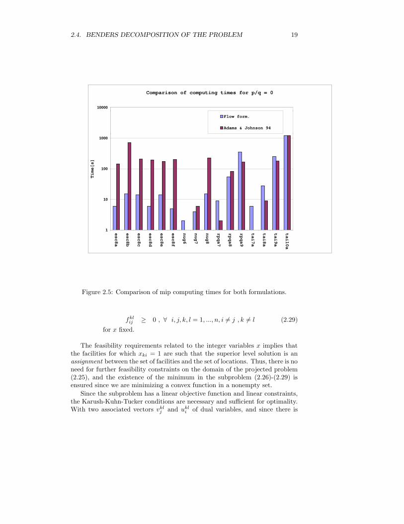
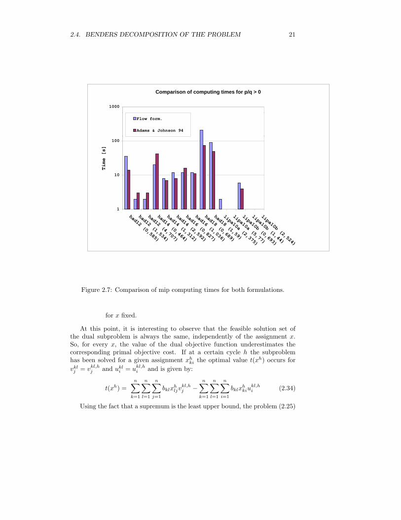
Tables 2.2, 2.3 and 2.4 presents the p/q ratio, and the computing times forthe flow formulation and Adams and Johnson [1] linearization (2.9) - (2.13).The entries on Tables 2.2, 2.3 and 2.4 assigned with ∗ are describing instancesnot solved in 24 hours of computation. In order to provide a better insight onanalysis, we have plotted these results on Figures (2.5), (2.6), (2.7) and (2.8),in logarithmic scale.
Original Problem Variables p/q Flow form. Adams and Johnsoninstance size Integer Continuous ratio time[s] time[s]esc8a 0 6 146esc8b 0 15 710esc8c 8 64 3136 0 14 207esc8d 0 6 196esc8e 0 14 176esc8f 0 5 202nug6 6 36 900 0 2 1nug7 7 49 1764 0 4 6nug8 8 64 3136 0 15 227rpqa7 7 49 1764 0 9 2rpqa8 8 64 3136 0 55 83rpqa9 9 81 5184 0 348 166tai7a 7 49 1764 0 6 1tai8a 8 64 3136 0 28 9tai9a 9 81 5184 0 247 178tai10a 10 100 8100 0 1197 1218
Table 2.2: Problem dimensions for test instances, number of integer and con-tinuous variables, p/q ratio and a comparison of integer mixed programmingcomputing times.
From Tables 2.2, 2.3 and 2.4, we can realize that the linear term on theobjective function is responsible for an expressive reduction of the computingtimes, sometimes of an order of magnitude. Beyond this, the flow formulationappears to balance two desirable qualities: a not so poor linear programmingbound, easy to solve.

2.3. THE QUADRATIC ASSIGNMENT PROBLEM 15
Original Problem Variables p/q Flow form. Adams and Johnsoninstance size Integer Continuous ratio time[s] time[s]chr12a 0.426 4 584chr12a 0.796 3 629chr12b 12 144 17424 0.383 5 516chr12b 0.592 3 492chr12c 0.314 3 803chr12c 0.662 4 1217chr15a 0.631 16 14209chr15a 0.856 6 10125chr15b 15 225 44100 0.726 36 77071chr15b 1.817 14 60452chr15c 0.944 19 3872chr15c 0.807 9 3058chr18a 0.564 116 *chr18a 18 324 93636 1.304 41 *chr18b 0.455 21 *chr18b 1.864 7 *chr20a 1.047 76 *chr20a 2.028 28 *chr20b 20 400 144400 0.824 47 *chr20b 1.702 10 *chr20c 1.056 108 *chr22a 0.304 138 *chr22a 22 484 213444 0.744 19 *chr22b 0.293 96 *chr22b 1.341 18 *
Table 2.3: Problem dimensions for test instances, number of integer and con-tinuous variables, p/q ratio and a comparison of mixed integer programmingcomputing times.
In fact, for the problems with linear installation profitabilities, for someinstances it is possible to find the integer optimal solution using our flow formu-lation before the completion of the linear programming solution of Adams andJohnson [1] formulation. The only class of test instances in which the flow for-mulation was defeated was for the instances had ∗ ∗, just those that has some ofthe poorest linear programming bounds. In despite of that, the flow formulationlack of performance decreases as the ratio p/q grows.
These observations clearly suggest the existence of an equilibrium point be-tween the bound quality and the cost to compute it. The natural conclusion hereis that Adams and Johnson formulation is so hard to solve that his good linearprogramming bounds are overcomed by the large computing times required toobtain them. Even in some purely quadratic instances it is possible to defeatAdams and Johnson computing times, as observed in Table 2.2.
We must also consider the solution of the modified versions of the instancesnug30 and ste36a, reported until now only by Anstreicher et al. [6], using largescale parallel computing. For certain conditions of the p/q ratio, these problemscould be solved in computing times not superior to one hour, as reported inTable 2.4.
Based on the former discussion and on the good solution times acquiredby our flow formulation, we introduce a Benders decomposition scheme for theproblem.
16 CHAPTER 2. ASSIGNMENT PROBLEMS
Original Problem Variables p/q Flow form. Adams and Johnsoninstance size Integer Continuous ratio time[s] time[s]had12 0.585 35 14had12 12 144 17424 1.534 2 3had12 4.707 2 3had14 0.464 20 42had14 14 196 33124 1.312 8 7had14 2.592 12 8had16 16 256 57600 0.827 12 16had16 1.036 12 11had18 18 324 93636 0.689 209 74had18 1.590 89 49lipa10a 2.375 2 1lipa10a 5.770 1 1lipa10b 10 100 8100 0.693 6 4lipa10b 1.440 1 1lipa10b 2.524 1 1nug12 2.401 3 110nug12 12 144 17424 3.621 3 30nug12 8.584 1 9nug15 0.990 61 1350nug15 15 225 44100 1.113 24 258nug15 2.981 5 94nug15 5.522 6 126nug20 0.434 1069 *nug20 20 400 144400 3.268 42 654nug20 4.477 80 799nug30 30 900 756900 0.769 2719 *nug30 1.358 1779 *scr10 10 100 8100 0.221 22 311scr10 0.414 7 95scr12 12 144 17424 0.188 146 13554scr12 0.336 54 6854ste36a 0.843 2896 *ste36a 36 1296 1587600 1.199 2801 *ste36a 1.871 2196 *tai10b 0.003 197 344tai10b 10 100 8100 0.013 96 714tai10b 0.023 95 658
Table 2.4: Problem dimensions for test instances, number of integer and con-tinuous variables, p/q ratio and a comparison of mixed integer programmingcomputing times.
2.4 Benders Decomposition of the Problem
Benders partitioning method was published in 1962 [17] and it was initiallydeveloped to solve mixed integer programming problems. The computationalsuccess of the method to solve large scale multi-commodity distribution sys-tem design models has been confirmed since the pioneering paper of Geoffrionand Graves [53]. Magnanti and Wong [89] proposed a methodology to improveBenders decomposition algorithm performance when applied for solving mixed-integer programs. They introduced a technique for accelerating the algorithmconvergence and developed a theory that distinguishes ”good” formulations forthose problems that have different, but equivalent, possible formulations. Wecan also remark the work of Geoffrion, on the generalized Benders method [52],and Balas and Bergthaller [10] revisiting the cut generation procedure. A Ben-ders partitioning method essentially relies on a projection problem manipulation,

2.4. BENDERS DECOMPOSITION OF THE PROBLEM 17
Comparison of LP bounds.
0
0,1
0,2
0,3
0,4
0,5
0,6
0,7
0,8
0,9
1
chr12a
chr12b
chr12c
chr15a
chr15c
had12
had14
lipa10a
nug12
nug15
nug5
nug6
nug7
nug8
scr10
scr12
tai10a
tai10b
tai5a
tai6a
tai7a
tai8a
tai9a
Bound Quality
Flow form.
Adams & Johnson 94
Figure 2.3: Comparison of linear programming bounds for both formulations.
that is then followed by the solution strategies of dualization, outer linearizationand relaxation.
Starting with the flow formulation described by equations (2.20) - (2.23),from the viewpoint of mathematical programming we can conceive a projectionof the problem onto the space of the assignment variables x, thus resulting thefollowing implicit problem to be solved at a superior level:
min −n
∑
k=1
n∑
i=1
akixki + t(x) (2.25)
subject to (2.1)-(2.3)
where t(x) is calculated by the following problem to be solved at an inferior

18 CHAPTER 2. ASSIGNMENT PROBLEMS
Comparison of LP computing times
1
10
100
1000
10000
100000
chr12a
chr12b
chr12c
chr15a
chr15c
had12
had14
lipa10a
nug12
nug15
nug5
nug6
nug7
nug8
scr10
scr12
tai10a
tai10b
tai5a
tai6a
tai7a
tai8a
tai9a
Time[s]
Flow form.
Adams & Johnson 94
Figure 2.4: Comparison of lp computing times for both formulations.
level:
t(x) = min
n∑
i=1
n∑
j=1
n∑
k=1
n∑
l=1
cijfklij (2.26)
subject to:
−n
∑
j=1
fklij = −bklxki , ∀ i, k, l = 1, ..., n, i 6= j , k 6= l (2.27)
n∑
i=1
fklij = bklxlj , ∀ j, k, l = 1, ..., n, i 6= j , k 6= l (2.28)
2.4. BENDERS DECOMPOSITION OF THE PROBLEM 19
Comparison of computing times for p/q = 0
1
10
100
1000
10000
esc8a
esc8b
esc8c
esc8d
esc8e
esc8f
nug6
nug7
nug8
rpqa7
rpqa8
rpqa9
tai7a
tai8a
tai9a
tai10a
Time[s]
Flow form.
Adams & Johnson 94
Figure 2.5: Comparison of mip computing times for both formulations.
fklij ≥ 0 , ∀ i, j, k, l = 1, ..., n, i 6= j , k 6= l (2.29)
for x fixed.
The feasibility requirements related to the integer variables x implies thatthe facilities for which xki = 1 are such that the superior level solution is anassignment between the set of facilities and the set of locations. Thus, there is noneed for further feasibility constraints on the domain of the projected problem(2.25), and the existence of the minimum in the subproblem (2.26)-(2.29) isensured since we are minimizing a convex function in a nonempty set.
Since the subproblem has a linear objective function and linear constraints,the Karush-Kuhn-Tucker conditions are necessary and sufficient for optimality.With two associated vectors vkl
j and ukli of dual variables, and since there is

20 CHAPTER 2. ASSIGNMENT PROBLEMS
Comparison of computing times for p/q > 0
1
10
100
1000
10000
100000
chr12a (0,426)
chr12a (0,796)
chr12b (0,383)
chr12b (0,592)
chr12c (0,314)
chr12c (0,662)
chr15a (0,631)
chr15a (0,856)
chr15b (0,726)
chr15b (1,817)
chr15c (0,807)
chr15c (0,944)
Time [s]
Flow form.
Adams & Johnson 94
Figure 2.6: Comparison of mip computing times for both formulations.
no duality gap for any x which forms an assignment, the optimal value of thesubproblem can be written as:
t(x) = max
n∑
k=1
n∑
l=1
n∑
j=1
bklxljvklj −
n∑
k=1
n∑
l=1
n∑
i=1
bklxkiukli (2.30)
subject to:
vklj − ukl
i ≤ cij , ∀ i, j, k, l = 1, ..., n, i 6= j, k 6= l (2.31)
vklj ∈ R , ∀ j, k, l = 1, ..., n, i 6= j, k 6= l (2.32)
ukli ∈ R , ∀ i, k, l = 1, ..., n, i 6= j, k 6= l (2.33)
2.4. BENDERS DECOMPOSITION OF THE PROBLEM 21
Comparison of computing times for p/q > 0
1
10
100
1000
had12 (0,585)
had12 (1,534)
had12 (4,707)
had14 (0,464)
had14 (1,312)
had14 (2,592)
had16 (0,827)
had16 (1,036)
had18 (0,689)
had18 (1,59)
lipa10a (2,375)
lipa10a (5,77)
lipa10b (0,693)
lipa10b (1,44)
lipa10b (2,524)
Time [s]
Flow form.
Adams & Johnson 94
Figure 2.7: Comparison of mip computing times for both formulations.
for x fixed.
At this point, it is interesting to observe that the feasible solution set ofthe dual subproblem is always the same, independently of the assignment x.So, for every x, the value of the dual objective function underestimates thecorresponding primal objective cost. If at a certain cycle h the subproblemhas been solved for a given assignment xh
ki the optimal value t(xh) occurs for
vklj = vkl,h
j and ukli = ukl,h
i and is given by:
t(xh) =
n∑
k=1
n∑
l=1
n∑
j=1
bklxhljv
kl,hj −
n∑
k=1
n∑
l=1
n∑
i=1
bklxhkiu
kl,hi (2.34)
Using the fact that a supremum is the least upper bound, the problem (2.25)

22 CHAPTER 2. ASSIGNMENT PROBLEMS
Comparison of computing times for p/q > 0
1
10
100
1000
10000
100000
nug12 (2,401)
nug12 (3,621)
nug12 (8,584)
nug15 (0,99)
nug15 (1,113)
nug15 (2,981)
nug15 (5,522)
nug20 (3,268)
nug20 (4,477)
scr10 (0,221)
scr10 (0,414)
scr12 (0,188)
scr12 (0,336)
tai10b (0,003)
tai10b (0,013)
tai10b (0,023)
Time [s]
Flow form.
Adams & Johnson 94
Figure 2.8: Comparison of mip computing times for both formulations.
is equivalent to the master problem:
min −n
∑
k=1
n∑
i=1
akixki + η (2.35)
subject to (2.1) - (2.3) and:
η ≥n
∑
k=1
n∑
l=1
n∑
j=1
bklxljvkl,hj −
n∑
k=1
n∑
l=1
n∑
i=1
bklxkiukl,hi , ∀h (2.36)
2.4. BENDERS DECOMPOSITION OF THE PROBLEM 23
1
2
3
4
5
6
1
2
3
4
5
6
= u kli + c ijv kl
j
= u kli + c ijv kl
j
= u kli + c ijv kl
j
= u kli + c ijv kl
j
= u kli + c ijv kl
j
= u kli + c ijv kl
j
ukli
Locations jLocations i
− cu = v klj
kli
− cu = v klj
kli
− cu = v klj
kli
− cu = v klj
kli
− cu = v klj
kli
= M
ji
ji
ji
ji
ji
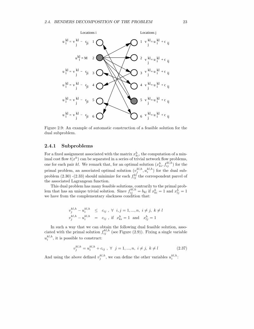
Figure 2.9: An example of automatic construction of a feasible solution for thedual subproblem.
2.4.1 Subproblems
For a fixed assignment associated with the matrix xhki, the computation of a min-
imal cost flow t(xh) can be separated in a series of trivial network flow problems,
one for each pair kl. We remark that, for an optimal solution (xhki, f
kl,hij ) for the
primal problem, an associated optimal solution (vkl,hj , ukl,h
i ) for the dual sub-
problem (2.30) -(2.33) should minimize for each fklij the correspondent parcel of
the associated Lagrangean function.This dual problem has many feasible solutions, contrarily to the primal prob-
lem that has an unique trivial solution. Since fkl,hij = bkl if xh
ki = 1 and xhlj = 1
we have from the complementary slackness condition that:
vkl,hj − ukl,h
i ≤ cij , ∀ i, j = 1, ..., n, i 6= j, k 6= l
vkl,hj − ukl,h
i = cij , if xhki = 1 and xh
lj = 1
In such a way that we can obtain the following dual feasible solution, asso-ciated with the primal solution fkl,h
ij (see Figure (2.9)). Fixing a single variable
ukl,hi , it is possible to construct:
vkl,hj = ukl,h
i + cij , ∀ j = 1, ..., n, i 6= j, k 6= l (2.37)
And using the above defined vkl,hj , we can define the other variables ukl,h
i :
24 CHAPTER 2. ASSIGNMENT PROBLEMS
ukl,hi = maxj , j 6=i [vkl,h
j − cij ] , ∀ i = 1, ..., n , i 6= j , k 6= l (2.38)
The systematic evaluation of the dual variables with meaningful values is aclue for an efficient implementation. Here, the two series of dual variables can beinterpreted as price information. Each variable vkl,h
j represents the commodityprice after flowing from facility k to facility l, if facility l is placed at location j.The variables ukl,h
i represents the commodity price before flowing from facilityk to facility l, if facility k is placed at location i.
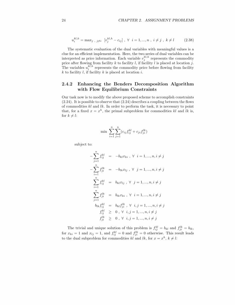
2.4.2 Enhancing the Benders Decomposition Algorithm
with Flow Equilibrium Constraints
Our task now is to modify the above proposed scheme to accomplish constraints(2.24). It is possible to observe that (2.24) describes a coupling between the flowsof commodities kl and lk. In order to perform the task, it is necessary to pointthat, for a fixed x = xh, the primal subproblem for commodities kl and lk is,for k 6= l:
min
n∑
i=1
n∑
j=1
(cijfklij + cjif
lkji )
subject to:
−n
∑
j=1
fklij = −bklxki , ∀ i = 1, ..., n, i 6= j
−n
∑
i=1
f lkji = −blkxlj , ∀ j = 1, ..., n, i 6= j
n∑
i=1
fklij = bklxlj , ∀ j = 1, ..., n, i 6= j
n∑
j=1
f lkji = blkxki , ∀ i = 1, ..., n, i 6= j
blkfklij = bklf
lkji , ∀ i, j = 1, ..., n, i 6= j
fklij ≥ 0 , ∀ i, j = 1, ..., n, i 6= j
f lkji ≥ 0 , ∀ i, j = 1, ..., n, i 6= j
The trivial and unique solution of this problem is fklij = bkl and f lk
ji = blk,
for xki = 1 and xlj = 1, and fklij = 0 and f lk
ji = 0 otherwise. This result leads
to the dual subproblem for commodities kl and lk, for x = xh, k 6= l:

2.4. BENDERS DECOMPOSITION OF THE PROBLEM 25
max bkl(
n∑
j=1
xljvklj −
n∑
i=1
xkiukli ) + blk(
n∑
i=1
xkivlki −
n∑
j=1
xljulkj )
subject to:
vklj + blkλkl
ij − ukli ≤ cij , ∀ i, j = 1, ..., n , i 6= j
vlki − bklλ
klij − ulk
j ≤ cji , ∀ i, j = 1, ..., n , i 6= j
vklj ∈ R , ∀ j = 1, ..., n, i 6= j
ukli ∈ R , ∀ i = 1, ..., n, i 6= j
Fixing at a reference value a single variable ukli and also a single variable
ulkj , making λkl
ij = 0 for i and j such that xhki = 1 and xh
lj = 1, it is possible towrite:
vkl,hj = ukl,h
i + cij , ∀ j = 1, ..., n
vlk,hi = ulk,h
j + cji , ∀ i = 1, ..., n
Using the above defined vkl,hj and vlk,h
i , we have for ukli and ulk
j :
ukl,hi − blkλkl,h
ij ≥ vkl,hj − cij , ∀ i, j = 1, ..., n, i 6= j
ulk,hj + bklλ
kl,hij ≥ vlk,h
i − cji , ∀ i, j = 1, ..., n, i 6= j
We must remark that, an enough high value of λklij can eventually increase
the value of ukl,hi while eventually decreasing the value of ulk,h
j . The idea hereis to decrease the value of any component of vector u as far as possible, butnever increasing the value of another component. Constructing a consistent dualsolution we have to fix, for instance, all the components of vector λh ≥ 0 as highas possible, while maintaining the idea of never increasing of any component ofvector uh:
ukl,hi = maxj , j 6=i [vkl,h
j − cij ] , ∀ i = 1, ..., n , i 6= j
And determining λkl,hij in such way that:
λkl,hij = 0 for index j that maximizes vkl,h
j − cij
λkl,hij =
1
blk(ukl,h
i − vkl,hj + cij) , ∀ i, j = 1, ..., n, i 6= j
After this step, we have a way to reduce some values of the origin prices ufor commodity lk:
26 CHAPTER 2. ASSIGNMENT PROBLEMS
ulk,hj = maxi , i6=j [vlk,h
i − bklλkl,hij − cji] , ∀ i = 1, ..., n, i 6= j
Now, we are ready to try out our decomposition algorithm over a set ofinstances, object of the next section.
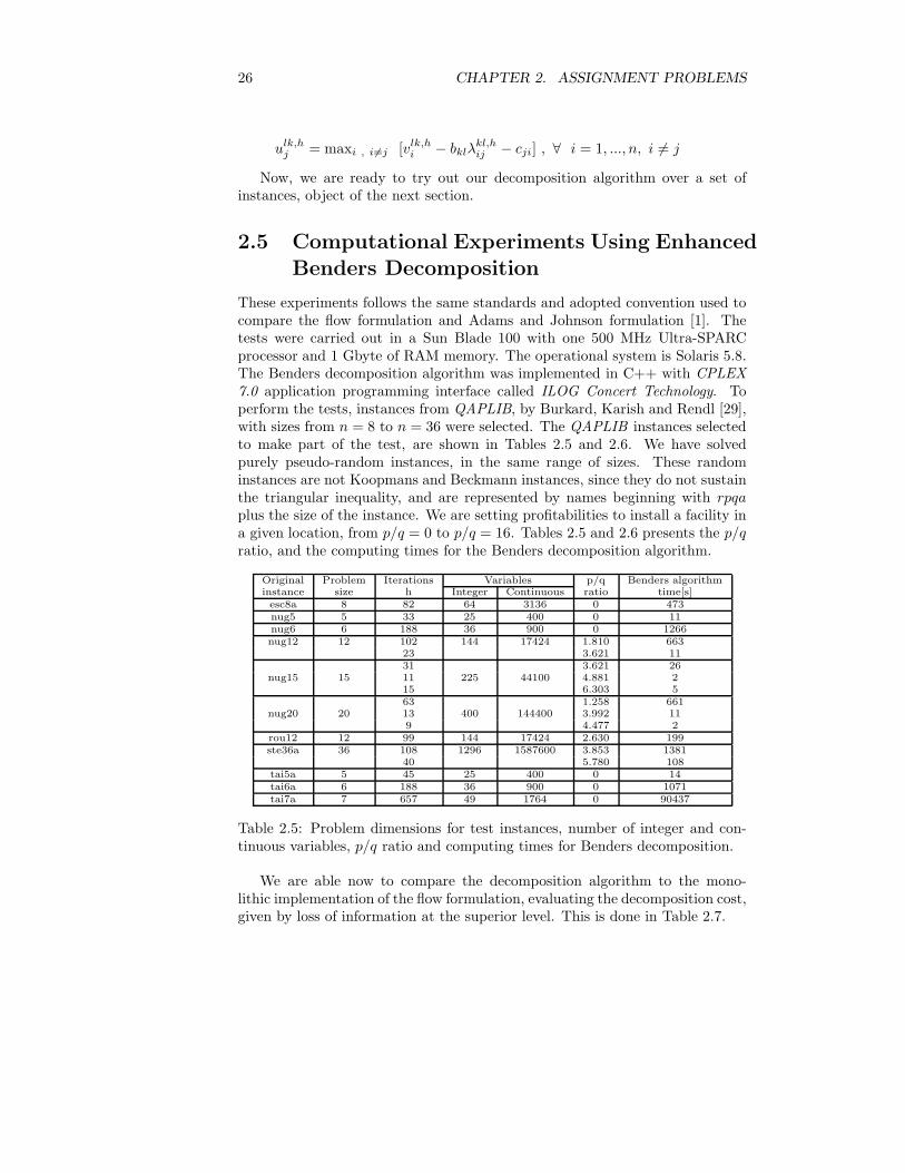
2.5 Computational Experiments Using Enhanced
Benders Decomposition
These experiments follows the same standards and adopted convention used tocompare the flow formulation and Adams and Johnson formulation [1]. Thetests were carried out in a Sun Blade 100 with one 500 MHz Ultra-SPARCprocessor and 1 Gbyte of RAM memory. The operational system is Solaris 5.8.The Benders decomposition algorithm was implemented in C++ with CPLEX7.0 application programming interface called ILOG Concert Technology. Toperform the tests, instances from QAPLIB, by Burkard, Karish and Rendl [29],with sizes from n = 8 to n = 36 were selected. The QAPLIB instances selectedto make part of the test, are shown in Tables 2.5 and 2.6. We have solvedpurely pseudo-random instances, in the same range of sizes. These randominstances are not Koopmans and Beckmann instances, since they do not sustainthe triangular inequality, and are represented by names beginning with rpqaplus the size of the instance. We are setting profitabilities to install a facility ina given location, from p/q = 0 to p/q = 16. Tables 2.5 and 2.6 presents the p/qratio, and the computing times for the Benders decomposition algorithm.
Original Problem Iterations Variables p/q Benders algorithminstance size h Integer Continuous ratio time[s]esc8a 8 82 64 3136 0 473nug5 5 33 25 400 0 11nug6 6 188 36 900 0 1266nug12 12 102 144 17424 1.810 663
23 3.621 1131 3.621 26
nug15 15 11 225 44100 4.881 215 6.303 563 1.258 661
nug20 20 13 400 144400 3.992 119 4.477 2
rou12 12 99 144 17424 2.630 199ste36a 36 108 1296 1587600 3.853 1381
40 5.780 108tai5a 5 45 25 400 0 14tai6a 6 188 36 900 0 1071tai7a 7 657 49 1764 0 90437
Table 2.5: Problem dimensions for test instances, number of integer and con-tinuous variables, p/q ratio and computing times for Benders decomposition.
We are able now to compare the decomposition algorithm to the mono-lithic implementation of the flow formulation, evaluating the decomposition cost,given by loss of information at the superior level. This is done in Table 2.7.

2.5. COMPUTATIONAL EXPERIMENTS USING ENHANCED BENDERS DECOMPOSITION27
Instance Problem Iterations Variables p/q Benders algorithmname size h Integer Continuous ratio time[s]
40 2.395 6737 2.412 56102 2.490 84247 2.667 9453 2.680 136
rpqa16 16 33 256 57600 2.701 5319 2.752 1220 4.158 1215 4.400 620 4.508 1217 4.583 874 3.261 82140 4.483 12442 4.496 14636 4.598 10131 4.731 7230 4.771 63
rpqa25 25 21 625 360000 5.194 3021 5.381 2911 5.767 626 5.801 4015 5.816 1120 6.071 2215 6.377 1121 3.037 5
rpqa9 9 6 81 5184 7.594 05 11.071 03 15.189 0
Table 2.6: Problem dimensions for test instances, number of integer and con-tinuous variables, p/q ratio and computing times for Benders decomposition.
Tables 2.8 and 2.9 presents an evolution of the computing times for Bendersdecomposition algorithm and for our monolithic implementation. These resultsare plotted in Figures (2.10), (2.11) and (2.12).
As one can see, the computing times for the flow formulation monolithicimplementation are sometimes better than those obtained by Benders decom-position scheme. The exception occurs on the situations that we deal with thelarger instances, with higher p/q ratios. This effect is due to the master problemstrengthening, that accelerates the lower bound progression.
We can sustain that high p/q ratios better describe the cost structure ofreal large scale implementations, and that the linear parcel, that represents theprofitability of a given location, can be considered in some cases more importantthan the transportation costs, from the economic point of view. This is speciallytrue when we think in location theory, since the linear term gives the profitabilityof a location for an economic activity. The economic equilibrium condition isso found for p/q = 1, and all situations where p/q > 1 capture liquid profit forthe considered optimal location for at least one activity. It is necessary to makeclear that our objective, when we start to develop the decomposition scheme,was to go were no one has gone before: proceed with the solution of largerinstances. This is impossible without decomposition since, for instances of sizebeyond 40, CPLEX crashes down due to lack of computer memory.
In fact, for large p/q ratios, it is possible to solve larger instances, without use

28 CHAPTER 2. ASSIGNMENT PROBLEMS
Original Problem Iterations Variables p/q Benders algorithm Flow form.instance size h Integer Continuous ratio time[s] time[s]chr12a 55 1.571 196 3chr12b 12 31 144 17424 2.555 59 4chr12c 81 2.374 736 4chr15a 142 1.383 3349 8chr15c 15 76 225 44100 2.191 1283 3chr15b 28 3.268 27 4nug15 15 9 225 44100 1.894 2 7nug20 20 30 400 144400 3.267 35 61nug30 30 44 900 756900 1.889 188 1236chr18a 18 68 324 93636 2.407 201 16chr18b 3 21.40 0 11chr20a 9 10.82 2 19chr20a 5 8.948 0 18chr20a 4 3.871 1 18chr20a 38 4.266 56 26chr20a 20 50 400 144400 4.728 99 20chr20b 4 10.75 0 20chr20b 4 6.854 1 20chr20b 15 4.069 6 20chr20b 45 2.268 65 22chr22a 22 69 484 213444 2.265 425 34had12 12 13 144 17424 2.531 4 3had14 14 25 196 33124 2.591 19 13had16 16 9 256 57600 1.035 2 12
Table 2.7: Problem dimensions for test instances, number of integer and contin-uous variables, p/q ratio and computing times for Benders decomposition andflow formulation.
of massive parallel computing, as can be seen in Table 2.10 where the computingwhere limited to 36 hours.
We are considering these results very expressive, since there is no solutionreport in the literature for any instance of size beyond 36, considering anyavailable formulation or algorithm. Since any extension of a NP-hard problemis also NP-hard, the addition of information about the external environment,trough the linear profitabilities, do not makes QAP easier, in a theoretical pointof view. This fact is confirmed by the computing times observed for the largerinstances (Table 2.10).
2.6 Concluding Remarks
On the cases where we can define or compute heterogeneous profitabilities, it ispossible to solve large instances of QAP , without an excessive computationalcost or the use of massive parallel computing. This conclusion has its founda-tions on the pioneer work of Koopmans and Beckmann and also on the workof Heffley, many years later. The inclusion of heterogeneous profits for locationis a natural step when considering location theory, and can introduce externalenvironment influence on the location decision process, being more realistic.
Once established this, the new flow formulation has proved to unify desirablequalities for a good mathematical programming implementation: be easy tosolve, giving good linear programming bounds. These two qualities are directly

2.6. CONCLUDING REMARKS 29
Evolution of computing times
0
5
10
15
20
2 4 6 8 10
p/q ratio
Time [s]
nug12 - flow
nug12 - Benders
nug15 - flow
nug15 - Benders
Figure 2.10: Evolution of computing times with p/q ratio.
responsible for the good computing times achieved, and also for the solution oflarger instances at reasonable cost, until now obtainable only trough the use ofcomputational grids.
For the instances of size beyond 40, the Benders decomposition algorithmappears to be the best choice to find an exact solution, avoiding excessive spaceand time complexity, if we observe some conditions about the cost structure.
For future work, it is necessary to better explore the equilibrium betweenbound quality and cost of computation, detecting when and how to merge easyto compute and stronger and hard to compute formulations for a given problem.

30 CHAPTER 2. ASSIGNMENT PROBLEMS
Evolution of computing times
0
20
40
60
80
100
120
2 3 4 5 6 7 8 9 10
p/q ratio
Time [s]
had16 - flow
had16 - Benders
had18 - flow
had18 - Benders
Figure 2.11: Evolution of computing times with p/q ratio.
p/q ratio 0 1 2 4Instance flow Benders flow Benders flow Benders flow Bendersnug12 * * 5 101 2 2 1 1nug15 * * 7 129 7 23 5 0nug20 * * 139 30751 55 13 52 8had14 * * 16 4 5 1 5 1had16 * * 12 27781 22 130 11 3had18 * * 31 3595 39 18 24 1chr15a * * 6 511 7 32 5 4chr15b * * 35 748 6 45 3 22chr15c * * 19 469 5 37 2 89chr18a * * 40 * 7 16 6 4ste36a * * 2821 * 2196 * 1971 952
Table 2.8: Evolution of computing times for Benders algorithm and the flowformulation
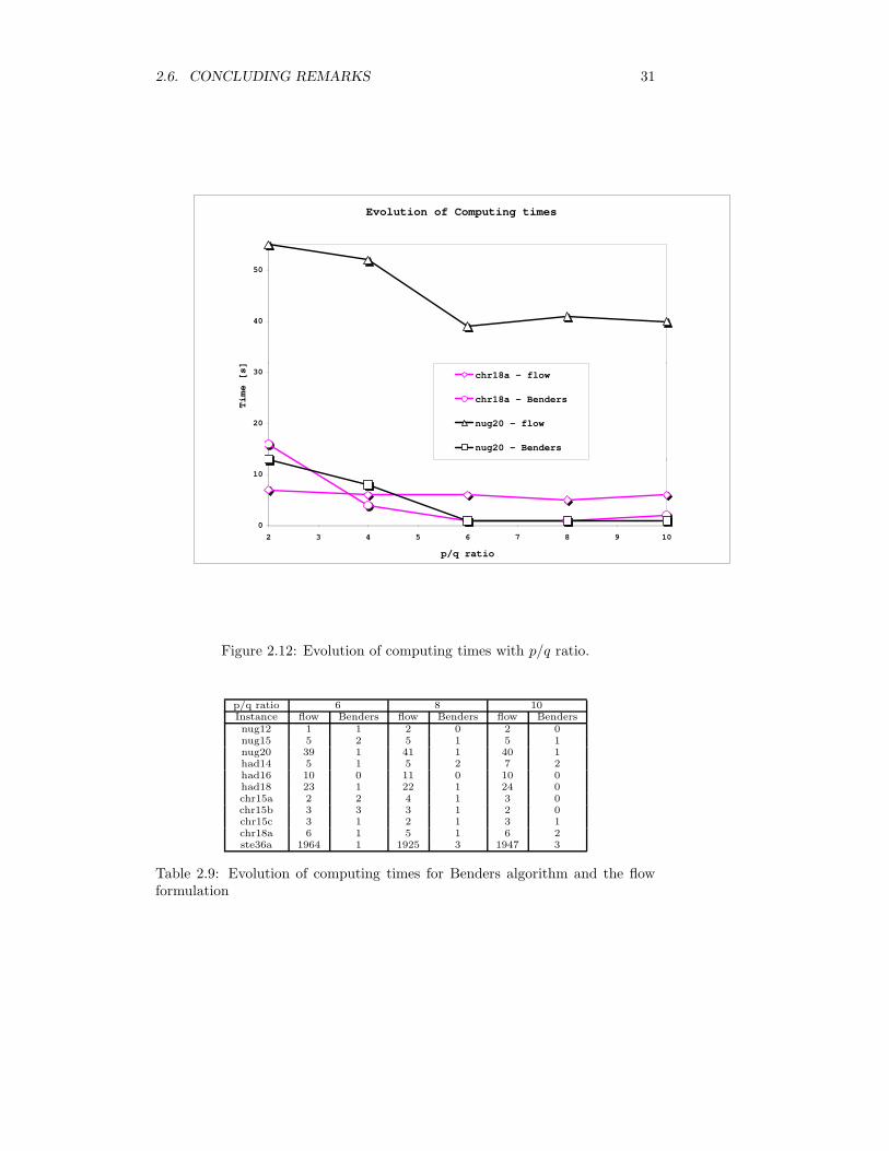
2.6. CONCLUDING REMARKS 31
Evolution of Computing times
0
10
20
30
40
50
2 3 4 5 6 7 8 9 10
p/q ratio
Time [s]
chr18a - flow
chr18a - Benders
nug20 - flow
nug20 - Benders
Figure 2.12: Evolution of computing times with p/q ratio.
p/q ratio 6 8 10Instance flow Benders flow Benders flow Bendersnug12 1 1 2 0 2 0nug15 5 2 5 1 5 1nug20 39 1 41 1 40 1had14 5 1 5 2 7 2had16 10 0 11 0 10 0had18 23 1 22 1 24 0chr15a 2 2 4 1 3 0chr15b 3 3 3 1 2 0chr15c 3 1 2 1 3 1chr18a 6 1 5 1 6 2ste36a 1964 1 1925 3 1947 3
Table 2.9: Evolution of computing times for Benders algorithm and the flowformulation
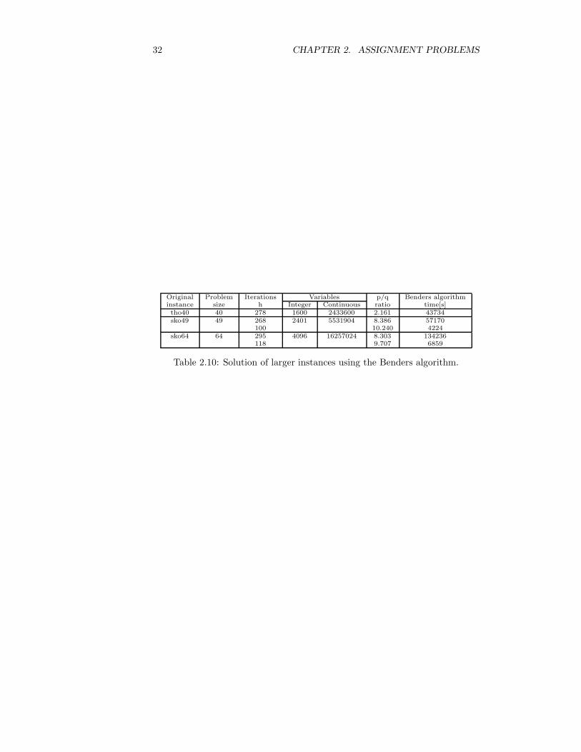
32 CHAPTER 2. ASSIGNMENT PROBLEMS
Original Problem Iterations Variables p/q Benders algorithminstance size h Integer Continuous ratio time[s]tho40 40 278 1600 2433600 2.161 43734sko49 49 268 2401 5531904 8.386 57170
100 10.240 4224sko64 64 295 4096 16257024 8.303 134236
118 9.707 6859
Table 2.10: Solution of larger instances using the Benders algorithm.
Chapter 3
The Placement of
Electronics with Thermal
Effects
3.1 Introduction
Nowadays, all the electronic and micro-electronic devices are migrating fromcontrolled environment places (laboratories, offices) to the direct applicationones (our houses, cars, and even clothes). This fact introduces a new elementin the product reliability equation: the capability of maintaining design con-ditions during operation. The engineers and designers are now facing a newchallenge: how to protect the most vulnerable parts of this kind of componentagainst damage on the application environments? They are dealing with hightemperatures, atmospheric residues, mechanical interference and vibration. Isit possible to create products which are just designed for maximum efficiencyand ignore these operational conditions? The answer seems to be no. In fact,reliability is a well known component of the quality function deployment.
It is important to remark that the heat transfer efficiency is a strong con-straint when designing more powerful computing machinery. This is a majorreason for the recent efforts on dealing with thermal problems on the micro-electronic domain, as can be seen in Lorente, Wechsatol and Bejan [81], Zuo,Hoover and Phillips [131], Visser and Kock [126] and Rocha, Lorente and Bejan[117]. The work of Wechsatol et al. [127] is a good reference on how networkflow models can be used to design an optimized distribution coolant network forelectronics systems. Several efforts have been done to obtain solutions that com-promise electronic components placement and temperature profiles, see Huanget al. [66], [65], [64] for MCM (Multi Chip Modules) design, and Queipo [113],[112]. For a more complete survey on the electronics cooling matter, we suggestto read Burmann et al. [30], Boyalakuntla and Murthy [22], Tucker [125], Ros-
33
34CHAPTER 3. THE PLACEMENT OF ELECTRONICS WITH THERMAL EFFECTS
ales et al. [118], EYK, Wen and Choo [100], Craig et al. [39] and Queipo et al.[111].
In order to overcome the problem, we must have a computer optimizationalgorithm which is capable of solving combinatorial placement problems in anefficient manner. It must be powerful enough to deal with the secondary met-ric — the thermal component. The exact optimization methods are not wellsucceeded in dealing with real size instances and the heat transfer associatedproblem is nonlinear and non-convex, although. In this work we design a Ben-ders decomposition based algorithm that is capable to solve exactly the place-ment problem keeping good solutions for the maximum temperature rising onthe surface board. The proposed algorithm is a heuristic. The models devel-oped by Queipo [113] and Huang [65] and our approach are very similar, butinstead of dealing with the thermal-placement combined problem with the aidof metaheuristcs, we are proposing a performance guarantee heuristic.
In section 3.2, the thermal model is developed and the temperature penaltyfunction is considered, being appreciated aspects involving the use of FiniteVolume Method [108] to solve the Energy Conduction Equation and the con-cerning boundary conditions. In section 3.3, the computational experimentsand the corresponding results are shown, where the test instances are viewed ina detailed way, resuming some concluding remarks and giving hints for futurework.
On the placement design of electronic boards, one needs to place n elec-tronic components to n established locations in a printed circuit card, buildingthe complete electronic board. As proposed by Steinberg (see [29]), it is inter-esting to minimize the distance among components which has greater levels ofinteractivity and energy or data flow, in order to avoid excessive signal delays.This is a location problem which can be modeled as an instance of the QAP. Onthe other hand, if all the major heat sources are put together, one can create aso called “hot-spot” on the board: a specific region of high energy dissipationthat causes usual heat sinks to present low efficiency. Then it becomes necessaryto investigate the sensitivity of optimal placement solution, when a new qualitycriterion is introduced: the maximal surface temperature.
3.2 Thermal Modeling and Temperature Penalty
Costs
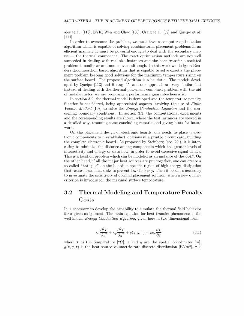
It is necessary to develop the capability to simulate the thermal field behaviorfor a given assignment. The main equation for heat transfer phenomena is thewell known Energy Conduction Equation, given here in two-dimensional form:
κz∂2T
∂z2+ κy
∂2T
∂y2+ g(z, y, τ) = ρcp
∂T
∂τ(3.1)
where T is the temperature [oC], z and y are the spatial coordinates [m],g(z, y, τ) is the heat source volumetric rate discrete distribution [W/m3], τ is

3.2. THERMAL MODELING AND TEMPERATURE PENALTY COSTS 35
the time [s], κ is the thermal conductivity [W/(oC · m)], ρ is the characteris-tic density [kg/m3] of the system and cp is the constant pressure specific heat[kJ/(oC · kg)]. This second order partial differential equation is subject in eachlateral side to the following boundary conditions:
−κzAz∂T
∂z|z=z1
= hconv1 Az(T − T∞)
−κzAz∂T
∂z|z=z2
= hconv2 Az(T − T∞) (3.2)
−κyAy∂T
∂y|y=y1
= hconv3 Ay(T − T∞)
−κyAy∂T
∂y|y=y2
= hconv4 Ay(T − T∞)
and to an initial condition like:
T |τ=τ0= T0 (3.3)
Here, hconvi , for each i = 1, 2, 3, 4, is the convective heat transfer coefficient
[W/(oC ·m2)] at each corresponding boundary. The natural and forced convec-tive heat transfer over the horizontal surface is included as a general negativesource term packed in g(z, y, τ), having the same form of (3.2), approximatingthe combined heat transfer coefficient by:
hconvsurface =
κ
L· 0.664 Re1/2 Pr1/3 (3.4)
where Re is the associated Reynolds Number, Pr is the Prandtl Number and Lis a fluid flow geometry dependent length [m]. To obtain good solutions for thismodel, we can use a simple version of the Finite Volume Technique [108]. In ourdiscretization, we are using a mesh nine times the size of the test instance (Fig-ure (3.1)). Only the two-dimensional isotropic steady state situation is underanalysis. The Central Difference Interpolating Scheme was adopted, and an av-erage heat source term in each volume is used to accomplish the discrete natureof heat source distribution. Since steady state heat conduction usually presentsgood solution properties for the associated Finite Volume equation set, we cannot observe numerical diffusion, instabilities or other numerical degradation atthis level of grid resolution. All the thermo-physical properties used to describethe thermal model are given in Table 3.1 (the boundary convective conditionswas chosen as typical values in electronics equipments [16], [123]).
3.2.1 Maximum Temperature and Penalty Costs
When solved, the thermal model (equations (3.1)-(3.4)) can determine the high-est temperature over the electronics board under investigation. It is interesting

36CHAPTER 3. THE PLACEMENT OF ELECTRONICS WITH THERMAL EFFECTS
Table 3.1: Thermo-physical properties for the thermal model.Environment Temperature 25 oCTotal Dissipated Power 120 WLateral Board Dimension (L) 0.20 mThermal Conductivity (Glass Fiber - Epoxy) 5.9 · 10−1 W/(m · K)Lateral Convective Heat Transfer Coefficients 1.0 · 10−4W/(m2 · K)
Finite Volum Grid
1 2 3 4 5 6
2
3
4
5
6
0.20 m.
Figure 3.1: QAP instance and Finite Volume Grid representation.
to remark that, for each fixed assignment x given by the master problem (2.35)-(2.36), see chapter 2, a different temperature field and maximum temperaturemust be found. Since the source term g(z, y, τ) is given by the power dissipa-tion of each electronic component being assigned to a given location, it is nottrivial to obtain analytical solution for (3.1)-(3.4), considering the discrete na-ture of the power source distribution over the board (in fact, this singularity isthe reason for the adoption of a Finite Volume technique). Beyond this, sincethe maximum temperature is not obtained explicitly, it is very difficult to es-tablish a function correlating the maximum temperature and the assignment x,becoming virtually impossible to ensure mathematical properties like convexity,discarding approaches via generalized Benders decomposition [52].
It is necessary to point that the maximum temperature over the electronicsboard under study is an important design variable, since it determines partially

3.2. THERMAL MODELING AND TEMPERATURE PENALTY COSTS 37
the reliability of the project on the application environment. If this tempera-ture is very high, an entire new cooling system for the electronics board canbe necessary, enhancing costs. Once defined a threshold, based on the designoperational conditions, we can conceive a penalty function. This function wouldbe responsible for taking into account the costs associated with maximum tem-peratures beyond the design established threshold, comprehending additionalmaintenance, cooling and environmental costs, for instance. In this case, wechoose to use the following function to play this role:
cTempraise =
0 , for Tmax < Tthreshold
µ(Tmax − Tthreshold)2 , for Tmax ≥ Tthreshold
(3.5)
0 20 40 60 80 100 120 140 160 180 200
0
100
200
300
400
500
600
700
Max. Temp. [Celsius]
Additional Cost [$]
Figure 3.2: The penalty overheating cost function, for a threshold temperatureof 85 Celsius.
Where cTempraise is the cost [$] associated with temperature raising Tmax beyond
the threshold Tthreshold, and µ is an estimative of additional cost unit per Celsiusdegree [$/oC2] (see Figure (3.2)). Unfortunately, even constructing (3.5) as aconvex function of Tmax, we remark that Tmax is not smooth or continuous,considering the assignment variables x. But, this also means that the Paretooptimal solution for the combined problem is always between the following twobounds: the lower-bound, given by the placement problem optimal solution,and the upper-bound, given by the placement problem optimal solution addedto the associated thermal cost component.

38CHAPTER 3. THE PLACEMENT OF ELECTRONICS WITH THERMAL EFFECTS
We can conceive now a performance guarantee heuristic to determine goodsolutions for the both point of views: thermal performance and placement cost.On the search for the optimal placement, we can examine the thermal costcomponent for each assignment solution, keeping the best upper bound. Whenthe optimal placement solution is found, we just choose the lowest total cost(the best upper bound), combining placement and thermal cost components.
Defining the combined thermal-placement problem lower bound as the opti-mal solution for QAP,
LB = QAPoptimal (3.6)
and the combined thermal-placement problem upper bound as the optimal so-lution for QAP plus the associated overheating penalty,
UB = QAPoptimal + cTempraise (3.7)
we can then pick the best feasible solution found
BEST = (QAP + cTempraise )best. (3.8)
At this point we remark that the performance guarantee of a heuristic algo-rithm for a minimization problem is α (α ≥ 1) if the algorithm is guaranteed todeliver a solution ϕ whose value is at most α times the optimal value: ϕ ≤ αϕ∗.Since we do not have the value of the global minimum for the combined thermal-placement problem (ϕ∗), we can only provide the following indirect relation:
LB ≤ ϕ∗, BEST ≤ αLB, BEST ≤ αϕ∗ where α = UB/LB.
This is true because cTempraise ≥ 0 by construction, and it is now possible to
define the optimality gap as:
GAP =BEST − LB
LB. (3.9)
An illustration of this method is depicted in Figure (3.3).
3.3 Computational Experiments
3.3.1 Experiment Description
When designing our computational experiments, we are interested on makingour test instances realistic. Following this objective, we can observe that therelationship between the system (the electronic board, in this case) and theapplication environment (external world connections, internal space restrictions,other interferences) has the same importance as the interrelations among thesystem components, being even more important sometimes.
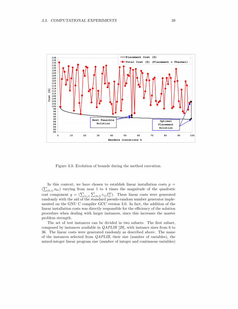
3.3. COMPUTATIONAL EXPERIMENTS 39
80828486889092949698
100102104106108110112114116118120122124126128130132134136138
0 10 20 30 40 50 60 70 80 90 100
Benders iterations h
Cost [$]
Placement Cost ($)
Total Cost ($) (Placement + Thermal)
Optimal Placement Solution
Best Feasible Solution
Figure 3.3: Evolution of bounds during the method execution.
In this context, we have chosen to establish linear installation costs p =(∑
(k,i) aki) varying from near 1 to 4 times the magnitude of the quadratic
cost component q = (∑
(i,j)
∑
(k,l) cijfklij ). These linear costs were generated
randomly with the aid of the standard pseudo-random number generator imple-mented on the GNU C compiler GCC version 3.0. In fact, the addition of thelinear installation costs was directly responsible for the efficiency of the solutionprocedure when dealing with larger instances, since this increases the masterproblem strength.
The set of test instances can be divided in two subsets. The first subset,composed by instances available in QAPLIB [29], with instance sizes from 6 to36. The linear costs were generated randomly as described above. The nameof the instances selected from QAPLIB, their size (number of variables), themixed-integer linear program size (number of integer and continuous variables)

40CHAPTER 3. THE PLACEMENT OF ELECTRONICS WITH THERMAL EFFECTS
and the Finite Volume grid size are shown in Table 3.2. The second subsetof test instances is also shown in Table 3.2, and it is composed by entirelyrandomly generated test instances, with sizes from 9 to 36. It is also possible tosee in Table 3.2 the component disposition over the electronics board surface.The column for component distribution shows how the n components are beingdisposed over the surface board. It is necessary to point that the thermo-physicalproperties and the board dimension are not being changed from one instance toanother. In this sense, when the instance size increases, we are just placing alarger number of smaller components.
Table 3.2: Test instances for computational experiments.Name Size Integer Variables Continuous Variables Fin. Vol. grid Component Distributionnug06 6 36 1296 54 3 × 2tail06 6 36 1296 54 3 × 2nug08 8 64 4096 72 3 × 2tail08 8 64 4096 72 4 × 2esc08a 8 64 4096 72 4 × 2esc08b 8 64 4096 72 4 × 2esc08c 8 64 4096 72 4 × 2esc08d 8 64 4096 72 4 × 2esc08e 8 64 4096 72 4 × 2esc08f 8 64 4096 72 4 × 2tail09 9 81 6561 81 3 × 3tail10 10 100 10000 90 5 × 2lipa10a 10 100 10000 90 5 × 2lipa10b 10 100 10000 90 5 × 2rou10 10 100 10000 90 5 × 2scr10 10 100 10000 90 5 × 2nug12 12 144 20736 108 4 × 3tail12a 12 144 20736 108 4 × 3rou12 12 144 20736 108 4 × 3scr12 12 144 20736 108 4 × 3nug20 20 400 160000 180 5 × 4ste36a 36 1296 1679616 324 6 × 6ste36b 36 1296 1679616 324 6 × 6rpqa9 9 81 6561 81 3 × 3rpqa16 16 256 65536 144 4 × 4rpqa25 25 625 390625 225 5 × 5rpqa36 36 1296 1679616 324 6 × 6
The intensity of each component heat source is a relative inter-activity mea-surement, defined as having a direct reason with the energy/information flowmatrix given on the instance under analysis, plus a small pseudo-random parcel.The heat sources were also adjusted to ensure physical consistency, resulting ontemperature ranges typically observed in electronics equipments. As the size ofthe instance is increased, the heat sources are redistributed in such way that thesame temperature ranges can be observed. We choose 85o Celsius as threshold,since we are designing an electronic board. The board under study is probablyused as host for semi-conductive devices as microchips, and over this temper-ature, must experience some performance loss. Referential values for the heatsource ranges and temperature threshold used here are available in [16] and[123]. The adopted value for the parameter µ in equation (3.5) was 5.

3.3. COMPUTATIONAL EXPERIMENTS 41
3.3.2 Numerical Results
Our computational experiments were carried out in a Sun Blade 100 Work-station equipped with a 500 MHz Ultra-SPARC processor and 1 Giga byte ofRAM memory, running Solaris 5.8. The Benders decomposition algorithm wasimplemented in C++, using ILOG CPLEX 7.0 Concert Technology applicationprogramming interface, on the solution of the master problem. Table 3.3 showsthe obtained results for the first set of tests, for the linear/quadratic cost ratiop/q kept between 1 and 2. This table lists instance name, instance size, numberof Benders iterations h, linear/quadratic cost ratio p/q for the optimal solution,Gap(%) as defined by equation (3.9) and the execution time. Tables 3.4 and3.5 points, respectively, to the second and the third sets of experiments. Forall these tables, the entries marked by ”*” could not be solved in 24 hours ofcomputing.
Table 3.3: Results for computational experiments - first set.Name Size h Optimal p/q cost ratio Gap (%) Time [s]nug06 6 9 1.25 0 10tail06 6 8 0.95 0 11nug08 8 12 1.13 8.3 120tail08 8 10 1.49 2.5 117esc08a 8 3 1.36 0 118esc08b 8 5 1.08 1.5 103esc08c 8 4 0.99 0.5 115esc08d 8 4 1.13 4.3 106esc08e 8 5 1.15 9.7 98esc08f 8 4 1.33 6.4 123tail09 9 20 1.18 12.1 305tail10 10 16 1.45 10.5 419lipa10a 10 30 1.34 5.4 383lipa10b 10 31 1.24 0.7 372rou10 10 32 1.19 8.2 385scr10 10 33 1.15 11.8 369nug12 12 37 1.45 33.1 521tail12a 12 26 1.14 25.6 483rou12 12 40 1.05 18.6 454scr12 12 30 1.12 30.5 427nug20 20 112 1.26 24.3 6019ste36a 36 * * * *ste36b 36 * * * *rpqa9 9 42 0.98 12.9 358rpqa16 16 105 1.61 15.4 464rpqa25 25 148 1.18 16.1 3348rpqa36 36 * * * *
It is possible to note in these three tables that the gap between solutions canbe responsible for a great amount of the total cost. Remembering that the heatsource distribution is partially randomly generated, we can observe that thereis no relation between the optimality gap and the size of the instance. This isalso true for the ratio p/q. Otherwise, the number of Benders iterations and thesolution time apparently reduces as the ratio p/q increases, as plotted in Figures(3.4) and (3.5) for the instances nug12 and nug20. In order to compare the dif-

42CHAPTER 3. THE PLACEMENT OF ELECTRONICS WITH THERMAL EFFECTS
Table 3.4: Results for computational experiments - second set.Name Size h Optimal p/q cost ratio Gap (%) Time [s]nug06 6 7 2.12 1.1 10tail06 6 8 2.87 0.8 12nug08 8 9 2.44 0.5 30tail08 8 5 2.72 0.7 109esc08a 8 3 2.6 2.1 32esc08b 8 4 2.94 0.6 64esc08c 8 2 2.55 0.9 86esc08d 8 2 2.46 0.7 7esc08e 8 2 2.24 1.7 42esc08f 8 4 2.11 1.3 35tail09 9 11 2.01 0.4 105tail10 10 12 2.57 0.6 296lipa10a 10 15 2.62 5.4 374lipa10b 10 16 2.63 0.3 340rou10 10 20 2.66 12.5 333scr10 10 16 2.05 11.8 298nug12 12 26 2.18 8.8 160tail12a 12 26 2.82 14.9 282rou12 12 22 2.64 11.3 351scr12 12 13 2.45 4.7 187nug20 20 60 2.85 8.3 981ste36a 36 237 2.58 22.1 1876ste36b 36 213 2.79 19.4 1381rpqa9 9 19 2.47 2.7 358rpqa16 16 54 2.23 12.3 464rpqa25 25 74 2.83 21.1 821rpqa36 36 348 2.76 28.7 2971
ference between only placement solutions and penalizing overheating solutions,Figures (3.6) and (3.7) show the temperature field over the board in both situa-tions. They correspond to the best solution for the instance ste36a consideringoverheating cost, and the temperature field for optimal QAP solution of ste36a.As we can see, the method was capable to find a solution that has a total costlower than optimal QAP solution. This solution designs a system that is colderthan the first one.
3.4 Concluding Remarks
In this paper, an approach to solve the electronic board design problem, de-scribed as a quadratic assignment problem instance, has been presented. An-other important quality solution criterion was under analysis: the maximaltemperature over the board surface. Methods to study the thermal field be-havior were discussed. The Benders decomposition algorithm was used as asolution technique to the proposed problem. The presented results report thatoverheating can respond for a great amount of the total cost, when considered.
It is interesting to remark that other quantities — depending on the selectedapplication — could be used as secondary quality criteria for the solution. Also,depending on other design parameters, many of other kinds of information could

3.4. CONCLUDING REMARKS 43
Table 3.5: Results for computational experiments - third set.Name Size h Optimal p/q cost ratio Gap (%) Time [s]nug06 6 2 3.02 0.1 4tail06 6 3 3.76 1.2 6nug08 8 3 3.29 9.0 2tail08 8 5 3.21 12.1 6esc08a 8 4 3.92 10.1 5esc08b 8 2 3.07 3.1 15esc08c 8 3 3.69 3.1 10esc08d 8 3 3.78 10.1 1esc08e 8 3 3.43 5.2 23esc08f 8 2 3.29 8.1 5tail09 9 5 3.16 7.0 77tail10 10 12 3.72 11.0 170lipa10a 10 10 3.42 17.3 124lipa10b 10 11 3.94 4.3 115rou10 10 12 3.21 5.6 162scr10 10 14 3.86 14.1 187nug12 12 16 3.55 3.0 93tail12a 12 12 3.48 2.2 105rou12 12 14 3.42 21.2 261scr12 12 8 3.84 12.1 119nug20 20 13 3.26 27.3 195ste36a 36 118 3.81 15.3 1379ste36b 36 147 3.99 27.2 1130rpqa9 9 8 3.27 5.4 14rpqa16 16 34 3.11 17.2 35rpqa25 25 53 3.75 21.2 379rpqa36 36 242 3.22 20.1 1234
be considered for this particular problem: for instance, the average and minimaltemperatures over the board.
For future work, it can be noted that a lot of real life problems can beviewed as instances of quadratic assignment problems and that it is sometimespossible to propose other quality criteria for the solution. Nowadays, this kindof solutions is valuable, since the environmental impact of any kind of largescale human implementation has becoming more important. It is desirable tohave the lower transport cost for intermediate commodities in the design of aregional industrial complex, and to take into account the dispersion of heavyindustrial atmospheric residues. There is no doubt that air quality is a greatpart of quality of life, and that environmental concerns must be in the top of thelist of all modern industrial management. One could still deal with the noiselevel of machinery on the low plant layout design.

44CHAPTER 3. THE PLACEMENT OF ELECTRONICS WITH THERMAL EFFECTS
0
20
40
60
80
100
120
1.2 1.7 2.2 2.7 3.2 3.7p/q cost ratio
Ben
der
s it
erat
ion
s
nug12
nug20
Figure 3.4: Number of Benders iterations versus p/q cost reason.
0
1000
2000
3000
4000
5000
6000
1.2 1.7 2.2 2.7 3.2 3.7p/q cost ratio
Exe
cuti
on
tim
e [s
]
nug12
nug20
Figure 3.5: Execution time [s] versus p/q cost reason.

3.4. CONCLUDING REMARKS 45
Figure 3.6: Temperature field for ste36a placement solution without overheatingpenalty.
Figure 3.7: Temperature field for ste36a placement solution considering over-heating penalty.

46CHAPTER 3. THE PLACEMENT OF ELECTRONICS WITH THERMAL EFFECTS

Chapter 4
The Local Access Network
Design With Congestion
Costs
4.1 Introduction
The tree network design problem consists of linking a supply node to its demandnodes to satisfy demands at minimal total cost. The problem may includeSteiner or transshipment nodes. Each arc of the network has three associatedcosts: a variable operational cost depending on the flow through the arc, anonlinear congestion cost that penalizes flows close to implicit capacities and afixed cost for setting up the physical connection represented by the arc.
This problem can be viewed as a generalization of the Steiner tree problemon a directed graph [85]. In fact, if we neglect variable costs at the arcs wewill have basically the Steiner problem, and in this sense we are treating aNP-hard problem, for which some computational strategies have been devised[87, 128, 67, 68, 75, 83]. On the other hand, if we neglect fixed costs on the arcswe have the single source transshipment problem, which can be solved easily[40].
As one can see, it is possible to use models for this problem to deal with anynetwork flow problem which has a single source tree as optimal solution. Thenetwork design problem associated with centralized computer networks and themulti-party multicast tree construction problem are good examples. The lastone has been treated with the aid of heuristics [69], but on the two versionstreated in the literature, the Single Source Tree Networks - where we have a trueroot of the multi-party multicasting tree - and the Core Based Tree Networks- where a single node, the core, is chosen to play a role as the tree root - it ispossible to accomplish the data to make the model faithful to the nature of theproblem. To make a survey on correlated research work, we refer to [58], [122]
47

48CHAPTER 4. THE LOCAL ACCESS NETWORK DESIGN WITH CONGESTION COSTS
and [72]. Congestioned computer networks are studied in the work of Ferreiraand Luna [42].
The provision of multi-point connections is one of most important servicesthat will be required in future broadband communication networks which sup-port distributed multimedia applications. Multimedia video-conferencing appli-cations, for example, requires that audio and video be transmitted to multipleconference participants simultaneously. This requires that an efficient multi-cast capability be provided by the underlying network. An illustration of theproblem is depicted in Figure 4.1.
Figure 4.1: The tree network design problem.
An alternative class of tree network design problems is related to the mini-mal spanning tree, where a central node has to be linked to all the remaindernodes in the network at minimal cost. These problems have been studied byauthors such as Gavish [47, 48, 49] and Gouveia [57]. This class of problemsincludes the capacitated and degree constrained minimal spanning tree prob-lems, and some routing and scheduling problems. In most of these problems allthe terminals have identical characteristics, and a single line type can be usedfor connecting the terminals. When the network has heterogeneous terminals,in the sense that they generate different amounts of traffic, and line costs thatare dependent of the line capacities we have the Telepak problem. In [48] Gav-ish proposes one-flow formulations for these problems and applies Lagrangean

4.2. MULTI-COMMODITY FLOW FORMULATION 49
relaxation with the sub-gradient optimization procedure to solve the degree con-strained minimal spanning tree problem, also solving the capacitated minimalspanning tree problem by Benders decomposition. In [49] a new formulation ofthe capacitated minimal spanning tree problem is presented as a zero-one in-teger programming problem and a combination of a sub-gradient optimizationprocedure and an augmented Lagrangean-based procedure is used to generatetight lower bounds. The original paper of Rothfarb and Goldstein [119] formu-lates the Telepak problem as a single commodity flow problem, and Gavish [48]shows that it can also be considered as a capacitated minimal spanning treeproblem. Several heuristics have been developed for the problem by Goldstein[56] and Chandy and Russel [35]. Gavish [50] presented a mixed-integer math-ematical programming formulation of the problem for a general cost structure.Hochbaum and Segev [63] propose two Lagrangean relaxations for the prob-lem and apply the sub-gradient optimization algorithm to approximate the bestLagrangean multipliers.
In the context of telecommunication systems the local access network de-sign problem corresponds to setting up a topology on an urban street networkthat minimizes the total cost of cables and underground piping infrastructurenecessary to link a switching center and its subscribers. Each subscriber grouphas a known demand and it is supposed that the switching center is able tosupply all subscribers demands. For each arc, the fixed cost is represented bythe underground infrastructure and the flow dependent cost is represented bythe cables to be installed in each arc. An optimal solution to this problem is atree with root at the switching center. Local access networks with aerial cablescan also be dealt with this formulation, and the fixed cost in such a case caninclude pole rents.
In a modern framework of applications, such as the multi-party multicast treeconstruction cited above, the fixed cost can be seen as a bandwidth leasing cost,due to the allocation of large capacity links used by multicasting participants.The variable costs, in this case, depends on data flow level and congestionlevel observed during the operation. The output is a low cost spanning treerepresenting the final computer conference configuration.
In Section 4.2 a mathematical programming formulation of the problem willbe presented. In Section 4.3 Benders decomposition is applied to the problem.The proposed solution was implemented and experimental results are reportedin Section 4.4. Section 4.5 closes this chapter with final remarks and conclusions.
4.2 Multi-commodity Flow Formulation
Consider a directed connected graph G(V, E), where V denotes the set of nodes,and E is a collection of arcs representing pairs of nodes between which a directtransmission link can be installed. Suppose we have an origin node o (the localhub or switching center) that must be linked to a number of |K| demand nodes(offices), each of them with a commodity flow requirement of dk where k ∈ Kand K ⊆ V . With appropriate structural, operational, leasing and congestion

50CHAPTER 4. THE LOCAL ACCESS NETWORK DESIGN WITH CONGESTION COSTS
costs, the problem is to find a minimal cost arborescence that links the switchingcenter to all the spatially distributed offices. It should be stressed that all flowsoriginate at a root node, i.e. the switching center or the server in a computernetwork.
4.2.1 Variables and Parameters
Define the variables:
xij =
1 if a directed transmission link is placed in arc (i, j)0 if not;
fijk : flow destined to demand node k, passing through arc (i, j);
gij : total flow of all commodities passing through arc (i, j).And also define the parameters:bij : fixed (structural) cost to install a directed transmission link in arc (i, j);
we suppose bij = β dij where dij is the distance (in meters) between i and j,and β is the linkage structural cost per meter.
cijk : variable (operational) cost to transmit one unit of commodity k througharc (i, j); we suppose cijk = γk dij , ∀k ∈ K.
The model allows variable costs to be dependent on both the commodity andthe arc. If the variable cost is independent from the commodity, we can makeγk = γ, ∀k. We also assume that, for each arc (i, j), is given an increasingfunction τij(gij) of the total flow passing through the arc. The leasing andcongestion cost function of the model is assumed to be separable with respectto arcs, and each parcel τij(gij) is intended to integrate quality of service andexpansion costs on arc (i, j). Quality of service is typically an increasing functionwhich measures congestion on the arc where commodities are considered ascompetitive users of a limited resource.
4.2.2 Mixed Integer Nonlinear Program
The mathematical model M is:
min∑
(i,j)∈E
[bijxij + τij(gij) +∑
k∈K
cijkfijk ] (4.1)
subject to:∑
k∈K
fijk − gij ≤ 0 , ∀(i, j) ∈ E (4.2)
−∑
(o,j)∈E
fojk = −dk , for node o and ∀k ∈ K (4.3)
∑
(i,k)∈E
fikk = dk , ∀k ∈ K (4.4)

4.2. MULTI-COMMODITY FLOW FORMULATION 51
∑
(i,j)∈E
fijk −∑
(j,l)∈E
fjlk = 0 , ∀j ∈ V − o and j 6= k and ∀k ∈ K (4.5)
fijk ≤ dk xij , ∀(i, j) ∈ E and ∀k ∈ K (4.6)
fijk ≥ 0 , ∀(i, j) ∈ E and ∀k ∈ K (4.7)
gij ≥ 0 , ∀(i, j) ∈ E (4.8)
xij ∈ 0, 1 , ∀(i, j) ∈ E (4.9)
The objective function (4.1) has three terms: the first one accounts for thetotal fixed cost of activating the arcs; the second term is a measure of leasing andcongestion costs related with the use of the arcs; and the third term is associatedwith the operational cost of sending flows of all commodities from the sourcenode to the demand nodes through the arcs. Constraints (4.2) account for thetotal flow of all the commodities passing through each arc (i, j). Constraints(4.3) ensure that the total flow of commodity k that originates from the sourcenode is equal to the demand of node k and constraints (4.4) impose that thetotal flow of commodity k arriving at demand node k is equal to its demand,dk. Constraints (4.5) ensure, for each commodity, the flow conservation for eachSteiner node of that commodity. The x and f coupling constraints (4.6) ensurethat no flow is allowed on arc (i, j) unless the fixed cost bij is paid. The factthat the flow of any commodity through an arc is not negative is guaranteedby constraints (4.7). Finally, constraints (4.9) state that the variables xij arebinary.
4.2.3 Theoretical Properties of the Linear and the Con-
cave Versions
It is important to note that the continuous relaxation of model M, that we callhere MLin, generates a quasi-integral polytope. A quasi-integral polytope is onein which the edges of the convex hull of its integer points are also edges of thepolytope itself [62]. This means that there exists a path through extreme integerpoints that finds the optimal integer solution, if it exists.
Another important theoretical property is that, for τij(gij) = 0, β = 0 anddk = 1, ∀k ∈ K the model is reduced to the multi-commodity flow formulationof the Steiner problem in directed graphs, as presented by Maculan and others[38, 129, 88, 55]. As a result, the strong formulation given by the objectivefunction (4.1) and constraints (4.3) to (4.9) also includes as particular case thelinear programming formulation for the shortest directed spanning tree problem,also introduced by Maculan [86]. All these theoretical properties can help tounderstand why, in many instances of this particular case, a linear programmingrelaxation of model M can automatically lead to optimal integral solutions.
Another related result concerns to the single source concave cost flow prob-lem, where τij(gij) is a concave cost function of the flow gij passing through thearc (i, j), with bij = 0 and cijk = 0 for every commodity k. For this particu-lar problem, it can be shown that a tree topology is associated to an optimalsolution for the problem [114].

52CHAPTER 4. THE LOCAL ACCESS NETWORK DESIGN WITH CONGESTION COSTS
4.2.4 Convexification of Leasing and Congestion Costs
As we can see in [51], to use the generalized Benders decomposition procedure,the Benders subproblem must be a convex one. The function choosed here torepresent congestion costs is the well known Kleinrock’s delay function, pre-sented by Gerla and Kleinrock in [54]. The possibility of capacity expansion ineach network link is accomplished with the aid of leasing costs for each capacity,remembering that the installation cost of first level of capacity is treated as afixed cost. In the framework of modern telecommunications systems or Internetmulti-party multicasting applications, the capacity expansion of a link can beseen as an upgrade of the bandwidth which can be made available for a groupof customers.
To manage this important feature together with the necessity of convexityin the Benders subproblem, we adopt here a convexification technique proposedin [84]. The cost function is assumed to be separable with respect to arcs and isintended to integrate quality of service (on the arc) and expansion cost. Qualityof service is typically an increasing function which measures congestion on thearc where commodities are considered as competitive users of a limited resource.
Let π1ij and π2
ij be the fixed costs of expanding the arc, to respectively,
capacities q1ij and q2
ij , τ0ij(gij), τ1
ij(gij) and τ2ij(gij) being the correspondent
congestion cost functions before and after expansions. Then, the integrated arccost function is defined on [0, q2
ij ] by:
σij(gij) = minτ0ij(gij), τ
1ij(gij) + π1
ij , τ2ij(gij) + π2
ij (4.10)
The univariate congestion functions τ 0ij(gij), τ1
ij(gij) and τ2ij(gij) are increas-
ing, proper convex, differentiable functions and depend, respectively, on the arccapacities q0
ij , q1ij and q2
ij (such that q0ij < q1
ij < q2ij). The derivatives τ0′
ij (gij),
τ1′
ij (gij) and τ2′
ij (gij) are increasing. We assume also the following hypothesis onthese functions:
τ0ij(0) = τ1
ij(0) = τ2ij(0) = 0 (4.11)
τ2ij(gij) < τ1
ij(gij) < τ0ij(gij), ∀gij ∈ (0, q2
ij) (4.12)
τ2′
ij (gij) < τ1′
ij (gij) < τ0′
ij (gij), ∀gij ∈ (0, q2ij) (4.13)
τ0′
ij (q0ij) ≥ Ω and τ1′
ij (q1ij) ≥ Ω and τ2′
ij (q2ij) ≥ Ω (4.14)
Observations:
1. Relation (4.11) trivially says that a null congestion cost results from a nullflow.
2. Relation (4.12) means that the congestion cost decreases when capacity isadded to an arc.
3. Relation (4.13) means that the marginal cost in an arc also decreases withthe addition of capacity.
4.3. BENDERS DECOMPOSITION OF THE PROBLEM 53
4. As the congestion increases with the flow, we force the derivative at thesaturation level to be greater than a given high value Ω in relation (4.14).
Figure 4.2 illustrates the integrated arc cost function σij(gij), as it is con-structed on the basis of the congestion functions τ 0
ij and τ1ij and τ2
ij and of the
fixed expansion cost π1ij and π2
ij . Remark that, from the properties (4.11-4.12),
when gij increases from 0, initially σij(gij) assumes the value of τ0ij(gij). Be-
cause of (4.13) the difference between the congestion costs τ 0ij(gij) and τ1
ij(gij)
increases until reaching the value π1ij , when a break-even point gij = ξ1 appears
with neither loss nor gain for expanding capacity. For gij > ξ1, it becomes moreeconomical to expand the arc capacity and the integrated function σij(gij) as-sumes the value of τ1
ij(gij) + π1ij , and for gij > ξ2, it is more economical to
expand arc capacity for q2ij and the function assumes the value of τ 2
ij(gij) + π2ij .
The values of the break-even points ξ1 and ξ2 are implicit in the solution ofthe equations τ0
ij(ξ1) = τ1ij(ξ1) + π1
ij and τ1ij(ξ2) = τ2
ij(ξ2) + π2ij . Figure 4.2 also
shows the convex hull function τij(gij) and the tangent points gij0 and gij2 of the
unique supporting line of σij on [0, q2ij ], in such a way that τ0′
ij (gij0) = τ2′
ij (gij2).The idea is that, for each specific class of convex functions satisfying properties(4.11-4.14), we can determine gij0, ξ1, ξ2 and gij2, thus characterizing explicitlythe convex hull, τij(gij), of the integrated function of congestion and expansioncosts, σij(gij). It results that problem MBend is a convex program for a fixednetwork topology, given by x, in such a way that we can conceive a Bendersdecomposition strategy to solve it.
4.3 Benders Decomposition of the Problem
Benders partitioning method was published in 1962 [17] and was initially devel-oped to solve mixed integer programming problems. The computational successof the method to solve large scale multi-commodity distribution system designmodels has been confirmed since the pioneering paper of Geoffrion and Graves[53]. Magnanti and Wong [89] proposed a methodology to improve Bendersdecomposition algorithm performance when applied to solve mixed-integer pro-grams. They introduced a technique for accelerating the algorithm convergenceand developed a theory that distinguishes ”good” formulations amongst dif-ferent, but equivalent, possible formulations. In [90] Benders decomposition isapplied to solve the uncapacitated network design problem and adapted to be asefficient as possible, when solving problems with undirected arcs. Now we spe-cialize the method to cope with nonlinear congestion costs and discrete capacityassignment. This is done as an application of generalized Benders decomposition[51] for an adequate variant of model M .
4.3.1 Problem Manipulations
Benders partitioning method essentially relies on a projection problem manipu-lation, that is then followed by the solution strategies of dualization, outer lin-

54CHAPTER 4. THE LOCAL ACCESS NETWORK DESIGN WITH CONGESTION COSTS
0 2 4 6 8 10 120
1
2
3
4
5
6
7
8
9
10
11
Tota
l Lin
k C
ost [d
olla
rs]
Total Amount of flow [Gbits/second]
The Convexified Resulting Integrated Cost Function
b ij
q 0
q 1
q 2
Figure 4.2: An example of convexified integrated leasing and congestion costfunction.
earization and relaxation. From the viewpoint of mathematical programmingwe can conceive a projection of problem M onto the space of the topologicalvariables x, thus resulting in the following implicit problem to be solved at asuperior level:
minx∈X
∑
(i.j)∈E
bij xij + v(x) (4.15)
where X = x | for x fixed there exist feasible flows satisfying (4.2) − (4.8)and where v(x) is calculated by the following problem to be solved at an inferiorlevel:
v(x) = min(f,g)∈G
∑
(i,j)∈E
[τij(gij) +∑
k∈K
cijkfijk ] subject to (4.6) for x fixed (4.16)
where G = (f, g) | f ≥ 0 and g ≥ 0 satisfying (4.2) − (4.5).The flow feasibility requirement related to a topological variable x ∈ X
implies that the components for which xij = 1 include an arborescence rooted

4.3. BENDERS DECOMPOSITION OF THE PROBLEM 55
at the origin o and destined to every demand node k ∈ K. Thus, there is noneed for further feasibility constraints on the domain of the projected problem(4.15), and the existence of the minimum in the subproblem (4.16) is assuredsince we are minimizing a convex function in a nonempty compact set.
Since the subproblem has a convex differentiable objective function and lin-ear constraints, the Karush-Kunh-Tucker conditions are necessary and sufficientfor optimality and the problem is amenable to dualization techniques [51]. Withan associated vector λ ≥ 0 of dual variables, the idea is to dualize the subprob-lem with respect to the coupling constraints (4.6). Since there is no duality gap,for any x ∈ X the optimal value of the subproblem 4.16 can be given by
v(x) = maxλ≥0
[ min(f,g)∈G
∑
(i,j)∈E
[τij(gij)+∑
k∈K
cijkfijk +∑
k∈K
λijk(fijk−dkxij)] (4.17)
or
v(x) = maxλ≥0
[∑
(i,j)∈E
∑
k∈K
−λijkdkxij + (4.18)
min(f,g)∈G
∑
(i,j)∈E
[τij(gij) +∑
k∈K
(cijk + λijk)fijk ]
The whole problem (4.15) is then equivalent to
minx∈X
∑
(i.j)∈E
bijxij + maxλ≥0
[∑
(i,j)∈E
∑
k∈K
−λijkdkxij+ (4.19)
min(f,g)∈G
∑
(i,j)∈E
[τij(gij) +∑
k∈K
(cijk + λijk)fijk ]
or, using the fact that a supremum is the least upper bound, problem (4.1) to(4.9) is equivalent to the master problem
mint,x∈X
∑
(i.j)∈E
bij xij + t (4.20)
subject to:
t ≥∑
(i,j)∈E
∑
k∈K
−λijk dk xij + (4.21)
min(f,g)∈G
∑
(i,j)∈E
[τij(gij) +∑
k∈K
(cijk + λijk)fijk ] for all λ ≥ 0
Generalized Benders decomposition solves problem (4.20)-(4.22) by the strat-egy of relaxation, i. e., ignoring all but a few constraints (4.22). If at a certain
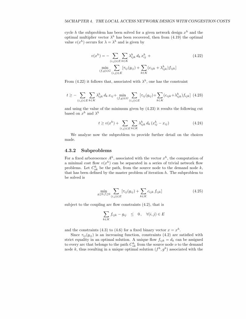
56CHAPTER 4. THE LOCAL ACCESS NETWORK DESIGN WITH CONGESTION COSTS
cycle h the subproblem has been solved for a given network design xh and theoptimal multiplier vector λh has been recovered, then from (4.19) the optimalvalue v(xh) occurs for λ = λh and is given by
v(xh) = −∑
(i,j)∈E
∑
k∈K
λhijk dk xh
ij + (4.22)
min(f,g)∈G
∑
(i,j)∈E
[τij(gij) +∑
k∈K
(cijk + λhijk)fijk ]
From (4.22) it follows that, associated with λh, one has the constraint
t ≥ −∑
(i,j)∈E
∑
k∈K
λhijk dk xij+ min
(f,g)∈G
∑
(i,j)∈E
[τij(gij)+∑
k∈K
(cijk+λhijk)fijk ] (4.23)
and using the value of the minimum given by (4.23) it results the following cutbased on xh and λh
t ≥ v(xh) +∑
(i,j)∈E
∑
k∈K
λhijk dk (xh
ij − xij) (4.24)
We analyze now the subproblem to provide further detail on the choicesmade.
4.3.2 Subproblems
For a fixed arborescence Ah, associated with the vector xh, the computation ofa minimal cost flow v(xh) can be separated in a series of trivial network flowproblems. Let Ch
ok be the path, from the source node to the demand node k,that has been defined by the master problem of iteration h. The subproblem tobe solved is
ming≥0,f≥0
∑
(i,j)∈E
[τij(gij) +∑
k∈K
cijk fijk ] (4.25)
subject to the coupling arc flow constraints (4.2), that is
∑
k∈K
fijk − gij ≤ 0 , ∀(i, j) ∈ E
and the constraints (4.3) to (4.6) for a fixed binary vector x = xh.Since τij(gij) is an increasing function, constraints (4.2) are satisfied with
strict equality in an optimal solution. A unique flow fijk = dk can be assignedto every arc that belongs to the path Ch
ok from the source node o to the demandnode k, thus resulting in a unique optimal solution (fh, gh) associated with the

4.3. BENDERS DECOMPOSITION OF THE PROBLEM 57
arborescence xh. The construction of an associated optimal multiplier vector canbe started with the dualization of the subproblem with respect to the couplingconstraints (4.2). With the correspondent dual variables θ ≥ 0, the optimalvalue v(xh) can be computed as
v(xh) = maxθ≥0
d(θ) (4.26)
where the dual function d(θ) is evaluated inducing the inherent separability ofeach commodity flows, since
d(θ) = ming≥0,f≥0
∑
(i,j)∈E
[τij(gij) +∑
k∈K
cijk fijk ] +∑
(i,j)∈E
θ(∑
k∈K
fijk − gij)
and so
d(θ) =∑
k∈K
minfk≥0
∑
(i,j)∈E
(cijk + θij)fijk +∑
(i,j)∈E
mingij≥0
(τij(gij) − θijgij) (4.27)
where each fk refers to the vector of commodity k flows that is feasible in thecorrespondent constraints (4.3) to (4.6) for x = xh.
We remark that, for an optimal solution (fh, gh) for the primal problem(4.25)-(4.2), an associated optimal solution θh for the dual problem (4.26) shouldminimize for each gij ∈ E the corresponding parcel of the Lagrangean functionin (4.27), what implies
θhij = τ ′(gh
ij) ∀(i, j) ∈ E (4.28)
As a consequence of fixing this unique optimal vector θh, we can now statein detail the primal-dual linear programming pair to be solved separately foreach commodity k ∈ K for any given xh.
Primal subproblem for commodity k when x = xh
min∑
(i,j)∈E
(cijk + θhij)f
hijk (4.29)
subject to:
−∑
(o,j)∈E
fhojk = −dk for the root o (4.30)
∑
(i,k)∈E
fhikk = dk (4.31)
∑
(i,j)∈E
fhijk −
∑
(j,l)∈E
fhjlk = 0 ∀j ∈ V − o and j 6= k (4.32)
−fhijk ≥ −dk xh
ij ∀(i, j) ∈ E (4.33)
fhijk ≥ 0 ∀(i, j) ∈ E (4.34)

58CHAPTER 4. THE LOCAL ACCESS NETWORK DESIGN WITH CONGESTION COSTS
The trivial and unique solution of the problem is:
fhijk =
dk if (i, j) ∈ Chok ⊆ Ah
0 otherwise(4.35)
Dual subproblem for commodity k when x = xh
The dual problem associated with the subproblem given by the objective func-tion (4.29) and constraints (4.30), (4.31), (4.32), (4.33) and (4.34) is:
maxph,λh≥0
dk(phkk − ph
ok −∑
(i,j)∈E
xhij λh
ijk) (4.36)
subject to:
phjk − ph
ik − λhijk ≤ cijk + θh
ij ∀(l, j) ∈ E (4.37)
This dual problem has many feasible solutions, contrarily to the primal prob-lem that has a unique trivial solution. Since fh
ijk = dk > 0 ∀(i, j) ∈ Chok ⊆ Ah
we have from the complementary slackness condition that:
phjk − ph
ik − λhijk = cijk + θh
ij ∀(i, j) ∈ Chok ⊂ Ah (4.38)
in such a way that we can construct, associated with the primal solution xh,the following dual feasible solution:
phok = 0 ∀k ∈ K, for the origin node o (4.39)
phjk = ph
ik + cijk + θhij , ∀(i, j) ∈ Ch
ok ⊂ Ah (4.40)
phik = p0
ik, ∀i ∈ V − V h (4.41)
λhijk = 0, ∀(i, j) ∈ Ch
ok ⊂ Ah (4.42)
λhijk = ph
jk − phik − cijk − θh
ij , ∀(i, j) ∈ E − Ah (4.43)
such that phjk − ph
ik > cijk + θhij
λhijk = 0, ∀(i, j) ∈ E − Ah such that ph
jk − phik ≤ cijk (4.44)
The systematic evaluation of the dual variables with meaningful commodityvalues is a clue for an efficient implementation. Here the two series of dualvariables can be interpreted as price information. Each variable ph
ik representsthe price of establishing communication k (k ∈ K) from the origin node o untilnode i (i ∈ V ) in iteration h (h = 1...H). On the other hand, each variable λh
ijk
gives for commodity k the value of an additional unit of capacity at arc (i, j) ∈ E.The dual variable λh
ijk evaluates for commodity k the maximal reduction in theoperational and leasing and congestion costs that could be gained with theintroduction of arc (i, j) in the solution. In the case of transportation systems,

4.3. BENDERS DECOMPOSITION OF THE PROBLEM 59
it can also be understood as a tax to be paid with the use of arc (i, j) in orderto maintain the distribution agents with no positive profit. Remark that thedual solution set (4.37) represents spatial prices for which there is no positiveprofit for any distribution agent that pays the cost cijk + θh
ij to ship commodityk through arc (i, j).
4.3.3 Master Problem
With the objective of producing a feasible solution from the master problem ofthe Benders decomposition method we have added some redundant constraintsto the model M. We call this extended model MBend. The new constraints tryto impose that the arcs implied by a solution to the master problem constitutea tree from the origin node o to all the demand nodes k ∈ K. Nevertheless,these constraints alone are not sufficient to guarantee this. For some probleminstances, a solution to the master problem can imply cycles in the generatedtopology and our algorithm treats this special situation accordingly. The re-dundant constraints are the following:
∑
(o,j)∈E
xoj ≥ 1 , for node o (4.45)
∑
(i,k)∈E
xik = 1 , ∀k ∈ K (4.46)
∑
(l,j)∈E
xlj −∑
(i,l)∈E
xil ≥ 0 , ∀l ∈ V − K − o (4.47)
∑
(i,l)∈E
xil ≥
∑
(l,j)∈E
xlj
∑
(l,j)∈E
1, ∀l ∈ V − K − o (4.48)
xij + xji ≤ 1 , ∀(i, j) ∈ E (4.49)
Constraint (4.45) imposes that at least one arc leaves the origin node. Con-straints (4.46) establish that only one arc arrives at each demand node. Con-straints (4.47) ensure that the number of arcs leaving a Steiner node is notsmaller than the number of arcs arriving at it. Constraints (4.48) express thefact that if at least one arc leaves node l, then at least one arc enters node l.Constraints (4.49) avoid the occurrence of cycles involving two arcs.
The master problem consists of searching for x variables with the followingobjective function:
min∑
(i,j)∈E
bijxij + t (4.50)
subject to the Benders cut constraints

60CHAPTER 4. THE LOCAL ACCESS NETWORK DESIGN WITH CONGESTION COSTS
t ≥ v(xh) −∑
(i,j)∈E
∑
k∈K
λhijk dk xij h = 0, 1, 2, ..., H (4.51)
and the constraints (4.45), (4.46), (4.47), (4.48), (4.49) and (4.9).We remark that the Benders cut constraint (4.51) results from (4.24) and
from the fact that∑
(i,j)∈E
∑
k∈K λhijk dk xh
ij = 0, since, by construction, at any
Benders cycle h, for any arc i, j ∈ E, either xhij = 0 or, from (4.42), λh
ijk = 0
for xhij = 1. The parameter H + 1 evaluates the number of cuts that can be
taken into account at each Benders iteration. For given h and k the number ofconstraints (4.51) provide a lower bound on the cost of the flow that leaves theorigin node to the demand node k. The variable t that appears in the objectivefunction (4.50) is the best known lower bound on the sum of operational costwith leasing and congestion costs.
4.3.4 Algorithm
The implemented Benders decomposition algorithm is presented below. Firstthe shortest path from the origin node to all the demand nodes and the minimumspanning tree of a reduced graph are computed. These two feasible solutions areused to initialize the dual variables. Next, in each cycle, one master problemand a series of subproblems are solved until the difference between the lowerand the upper bound becomes small enough, for a given tolerance parameter.The steps of the algorithm are the following:
1. Use Dijkstra’s algorithm to find the shortest path from the origin o toevery node of the network. Let E0 be the arcs of the arborescence thatcontains the shortest paths to all the nodes and let T (V 0, A0) be thecorresponding arborescence that links the origin o to all demand nodesk ∈ K (x0
ij = 1 ∀(i, j) ∈ A0 and x0ij = 0 ∀(i, j) ∈ E − A0). Make
p0ok = 0 ∀k ∈ K , for the origin node o
p0jk = p0
ik + cijk + θ0ij ∀(i, j) ∈ A0, ∀k ∈ K
p0jk = p0
ik + cijk ∀(i, j) ∈ E0 − A0, ∀k ∈ K
λ0ijk = 0 ∀(i, j) ∈ E0, ∀k ∈ K
Compute the cost associated with T (V 0, A0) (the sum of the fixed costof the arcs in A0 plus the sum of the variable costs for sending the flowrequirement of each commodity k from the origin o to the demand nodek). This value gives an initial upper bound, UB =
∑
(i,j)∈A0 bijx0ij +
∑
k∈k dkp0kk , and (x0, f0) is an incumbent solution. Also, the shortest
paths solution provides the minimal total variable cost among all possiblearborescences, and thus we can use it to initialize a lower bound, LB =∑
k∈k dkp0kk .
4.3. BENDERS DECOMPOSITION OF THE PROBLEM 61
2. Use Prim’s algorithm to find a minimal spanning tree in a reduced graphthat contains only the origin and the demand nodes k ∈ K. This re-duced graph is constructed as proposed by Mehlhorn in [95] using a singleshortest-path computation. Let T (V 1, A1) be the associated Steiner ar-borescence, that is contained in the original graph G(V, E), and that linksthe origin o to all demand nodes k ∈ K (x1
ij = 1 ∀(i, j) ∈ A1 and x1ij =
0 ∀(i, j) ∈ E − A1). C1ok is the set of the arcs in the path from the origin
to the demand node k through A1. Set the iteration counter h = 1.
3. Compute the values of the dual variables as indicated by the equations(4.39)-(4.44). A new value for the upper bound is calculated and if thisvalue is less than the current upper bound then the current upper boundis updated. Add a new cut to the master problem.
4. Solve the master problem. It provides a lower bound for the problem.If the upper bound is close enough to the lower bound, for the giventolerance, then stop.
5. Solve the subproblem. To solve it, initially verify if the arcs selected inthe master problem imply an arborescence from the origin to all demandnodes. If yes, set h = h + 1, let T (V h, Ah) be the arborescence that linksthe origin o to all demand nodes k ∈ K, contained in the original graphG(V, E), let Ch
ok be the set of the arcs in the path from the origin to thedemand node k through Ah, and go to step 3. Else, the topological solutionof the master problem is infeasible in the subproblem in the sense that itgenerates a cycle. In this case, the cycle is identified and a constraints toavoid it is added to the master problem model and no new lower bound isgenerated. To identify the cycle in the path from the origin to a demandnode, a backward search from the demand node is executed until a nodeis repeated. Let n be this node. A cycle avoiding constraint is generatedconsidering the arcs from the demand node to n in both directions. Thesum of the variables xij corresponding to these arcs must not be greaterthan the number of arcs from the demand node to n (considering only onedirection of the arcs and the second time that n is found). After the cycleavoiding constraints are added, the master problem must again be solved,then go to step 4.
4.3.5 Avoiding Cycles
As it was explained earlier, the model MBend uses the constraints (4.45 - 4.49) toaccomplish the necessity of computing a feasible solution at the higher (masterproblem) level which, in this case, is a tree. We use this redundant constraintsto guarantee the feasibility of flow balance and avoid to use type 2 cuts inBenders decomposition (extremal rays). However, depending on the demandvector structure and on the network connectivity level, constraints (4.45 - 4.49)are not powerful enough to ensure the calculation of a structural solution whichprevents cycles in the source/demand path.

62CHAPTER 4. THE LOCAL ACCESS NETWORK DESIGN WITH CONGESTION COSTS
This explains the use, just in case, of the strategy described on step 5 of thealgorithm given in the last subsection. This strategy is no more but the inclusionof a type 2 cut, and the consequent loss of one master problem iteration, justto ensure feasibility. Depending on the instance to be solved, this strategy maybe responsible for unnecessary computational effort.
To deal with this, we devise an alternative strategy, which preserves the flowbalance at the higher level without the necessity of constraints (4.45 - 4.49).This approach just uses the link between variables fijk and gij , as implied byconstraint (4.2), to construct a new master problem. Instead of working onlyin the space of topological variables x, in this new formulation we work in thespace of both the x and g variables, in such a way that the model is able toavoid cycles because it sustains the flow balance. We call this model MMBend,and the new master problem is plotted below.
min∑
(i,j)∈E
bijxij + t (4.52)
subject to:
−∑
(o,j)∈E
goj = −∑
k∈K
dk (4.53)
∑
(i,k)∈E
gik −∑
(k,j)∈E
gkj = dk , ∀k ∈ K (4.54)
∑
(i,j)∈E
gij −∑
(j,l)∈E
gjl = 0 , ∀j ∈ V − K − o (4.55)
gij ≤∑
k∈K
dk xij , ∀(i, j) ∈ E (4.56)
gij ≥ 0 , ∀(i, j) ∈ E (4.57)
xij ∈ 0, 1 , ∀(i, j) ∈ E (4.58)
and the Benders Cut:
t ≥ v(xh) −∑
(i,j)∈E
∑
k∈K
λhijk dk xij h = 0, 1, 2, ..., H (4.59)
With this model, we force the flow balance at the master level, with con-straints (4.53)-(4.57), and guarantee the feasibility on the structural variables x.On the other hand, the number of variables being treated by the master problemincreases by |E|. This is also onerous, but, for larger amounts of products beingshipped, may justify the alternative decomposition strategy.
4.4 Computational Results
Computational tests were carried out in a Sun Blade 100 with a 500 MHzUltra-SPARC processor and 1 Gbyte of RAM memory. The operational system

4.4. COMPUTATIONAL RESULTS 63
is Solaris 5.8. The Benders decomposition algorithm was implemented in C withGLPK 3.1 [91] application programming interface.
Table 4.1 shows the dimensions of the networks and of the correspondingmixed integer programming formulations for the tested problems. The testproblems can be divided into three classes: the first class contains problemsthat are Euclidean graphs randomly generated using a procedure similar tothat presented in [3]. This procedure has been used extensively for creatingtesting instances of the Steiner problem. The second class was based in dataobtained from a geographical information system and uses realistic costs anddistances based on different locations of Brazil. The third class of problemsrefers to some of Beasley’s graphs [15] for Steiner Problems. We have chosen asthe origin node the first demand node of each selected Beasley’s graph, and wehave assigned one unit of flow for each of the remainder demand nodes. Theseproblem instances were selected to perform a direct extension of the work ofRandazzo and Luna [116].
Problem Number of Variables in Model MNumber |V | |E| |K| β/γ Integer Continuous
1 12 36 3 1 36 1082 16 30 4 1 30 1203 16 60 4 1 60 2404 20 60 3 1 60 1805 25 80 4 1 80 3206 30 90 5 1 90 450
CLASS 7 35 100 6 1 100 6001 8 40 110 7 1 110 770
9 46 120 8 1 120 96010 50 130 8 1 130 104011 55 140 8 1 140 112012 60 150 9 1 150 135013 65 170 10 1 170 170014 70 200 12 1 200 240015 80 220 12 1 220 264016 10 21 8 10 21 16817 12 26 10 10 26 26018 14 31 12 10 31 37219 16 36 14 10 36 504
CLASS 20 18 40 16 10 40 6402 21 20 48 18 10 48 864
22 21 52 19 10 52 98823 22 55 20 10 55 1 10024 24 47 22 10 47 1 03425 25 50 20 10 50 1 000B1 50 126 8 10 126 1 008B2 50 126 12 10 126 1 512
CLASS B5 50 200 12 10 200 2 4003 B6 50 200 24 10 200 4 800
B16 100 200 16 10 200 3 200
Table 4.1: Network Dimensions for Test Problems.
Six different experiments were conducted to verify the algorithm performanceand to determine the behavior of the solutions founded as the network loadincreases. In order to create the arc cost function for the problem instancespresented in Table 4.1, six levels of implicit capacities were proposed (q0
ij , ..., q6ij),
and five expansion costs also (π1ij , ..., π
5ij). The implicit capacity level q0
ij wasdefined ad hoc and capacity levels 1 to 5 were produced just doubling the arc

64CHAPTER 4. THE LOCAL ACCESS NETWORK DESIGN WITH CONGESTION COSTS
capacity at each expansion level. Indexing the implicit capacity level by l,wehave
ql+1ij = 2 ql
ij , ∀i, j ∈ E , l = 0, ..., 5 (4.60)
The capacity expansion costs (π1ij , ..., π
5ij) were proposed in a non-increasing
realistic way, enabling scale economies for higher capacity levels. Another re-striction imposed over the expansion costs determines that their sum cannot begreater than 50% of the fixed arc instalation cost bij .
The main difficulty in this phase of our work was the unavailability of otherpopular methods for solving mixed integer nonlinear programs. This makesa comparison of optimal methods hard to obtain. We so choose to comparebetween linear and nonlinear versions of the test instances. The linear versionswere obtained setting the congestion costs equal to zero. This little exercise isable to shows us how different are the linear and nonlinear solutions.
The gap between linear and nonlinear solutions was defined by
GAP = 100
(
Optimumnonlinear − Optimumlinear
Optimumlinear
)
(4.61)
In our first experiment, the demand vector of each instance was chosento guarantee a low level of network load, leading to arc flows below the firstimplicit capacity level. The computational effort was due to the execution ofthe 30 problem instances proposed in Table 4.1 using the formulations MBend,MMBend and a linear run obtained setting congestion costs equal to zero.
To produce the second experiment, all demand vectors were multiplied by afactor of two, and this process was repeated six times, in order to generate datafor all the six experiments under focus. With this policy, we have incrementedthe total network load beyond a factor of twelve. With each of the 30 probleminstances being tested for six different levels of network load, using formulationsMBend, MMBend and the linear version, we have 540 different runs.
However, the first five experiments has presented an analogous behavior,always deriving the same optimal structure for linear an nonlinear instances.Beyond this, the gap observed between linear and nonlinear results was almostthe same for experiments 1 to 5, as well as the numbers of Benders iterationsand the computing times.
For the gap between nonlinear and linear solutions, this can be explained bythe following effect: allowing six levels of expansion for the implicit capacities,the tangent point gij0 used to define the unique supporting line (convex hull) ofthe integrated arc cost function is located very near to zero. In this case, evensmall arc flows are computed with the aid of the linear portion of the convexapproximation. Combining the effect described above with the economies ofscale suggested by the existent relationship between parameters β and γ, itis possible to conclude that we are always obtaining as optimal solution anarborescence that is very much like the shortest path tree or the minimumspanning tree. This tendency is repeated until the network load level becomescloser to the maximum installed capacity q5
ij , where the congestion costs become
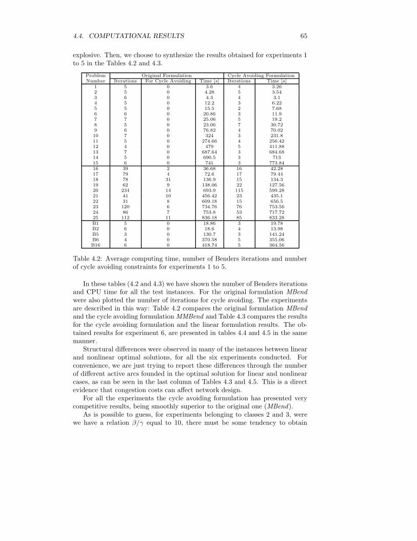
4.4. COMPUTATIONAL RESULTS 65
explosive. Then, we choose to synthesize the results obtained for experiments 1to 5 in the Tables 4.2 and 4.3.
Problem Original Formulation Cycle Avoiding FormulationNumber Iterations For Cycle Avoiding Time [s] Iterations Time [s]
1 5 0 3.6 4 3.262 5 0 4.28 5 3.543 6 0 4.3 4 3.14 5 0 12.2 3 6.225 5 0 15.5 2 7.686 6 0 20.86 3 11.97 7 0 25.06 5 19.28 5 0 23.06 7 30.729 6 0 76.82 4 70.0210 7 0 324 3 231.811 5 0 274.66 4 256.4212 4 0 479 5 411.8813 7 0 687.64 3 684.6814 5 0 690.5 3 71315 6 0 741 3 773.8416 39 2 36.68 16 42.2817 79 4 72.6 17 79.4418 78 31 136.9 15 134.319 62 9 138.06 22 127.5620 234 14 693.9 115 599.2821 41 10 456.42 23 435.122 31 8 609.18 15 656.523 120 6 734.76 76 753.5624 86 7 753.8 53 717.7225 112 11 836.18 85 833.28B1 5 0 18.86 3 19.78B2 6 0 18.6 4 13.98B5 3 0 130.7 3 141.24B6 4 0 370.58 5 355.06B16 6 0 418.74 5 364.56
Table 4.2: Average computing time, number of Benders iterations and numberof cycle avoiding constraints for experiments 1 to 5.
In these tables (4.2 and 4.3) we have shown the number of Benders iterationsand CPU time for all the test instances. For the original formulation MBendwere also plotted the number of iterations for cycle avoiding. The experimentsare described in this way: Table 4.2 compares the original formulation MBendand the cycle avoiding formulation MMBend and Table 4.3 compares the resultsfor the cycle avoiding formulation and the linear formulation results. The ob-tained results for experiment 6, are presented in tables 4.4 and 4.5 in the samemanner.
Structural differences were observed in many of the instances between linearand nonlinear optimal solutions, for all the six experiments conducted. Forconvenience, we are just trying to report these differences through the numberof different active arcs founded in the optimal solution for linear and nonlinearcases, as can be seen in the last column of Tables 4.3 and 4.5. This is a directevidence that congestion costs can affect network design.
For all the experiments the cycle avoiding formulation has presented verycompetitive results, being smoothly superior to the original one (MBend).
As is possible to guess, for experiments belonging to classes 2 and 3, werewe have a relation β/γ equal to 10, there must be some tendency to obtain

66CHAPTER 4. THE LOCAL ACCESS NETWORK DESIGN WITH CONGESTION COSTS
Problem Cycle Avoiding Formulation Linear Results Nonlinear/linear Number ofNumber Iterations Time [s] Iterations Time [s] GAP (%) Different Arcs
1 4 3.26 5 3.3 24.742 22 5 3.54 6 2.92 25.94 43 4 3.1 4 3.28 15.386 34 3 6.22 5 7.08 26.096 25 2 7.68 5 7.86 25.91 36 3 11.9 5 14.34 25.25 37 5 19.2 7 18.58 24.818 48 7 30.72 7 25.42 24.532 39 4 70.02 4 72.68 16.912 310 3 231.8 5 217.4 24.764 511 4 256.42 7 244.12 25.138 312 5 411.88 4 432.8 26.65 313 3 684.68 7 618.76 25.824 614 3 713 5 700.8 24.642 415 3 773.84 5 789.4 25.012 216 16 42.28 19 45.32 26.23 517 17 79.44 18 82.44 24.96 418 15 134.3 19 118 25.784 419 22 127.56 27 118.48 24.456 220 115 599.28 116 573.52 34.728 321 23 435.1 28 416.58 25.63 622 15 656.5 21 621.88 25.896 523 76 753.56 77 799.96 16.188 324 53 717.72 56 763 25.558 225 85 833.28 93 854.94 24.434 6B1 3 19.78 5 18.96 25.788 6B2 4 13.98 6 15.98 14.788 5B5 3 141.24 3 160.98 24.948 5B6 5 355.06 3 358.18 34.822 3B16 5 364.56 3 367.58 25.954 6
Table 4.3: Average computing time, number of Benders iterations, Nonlin-ear/linear gap and number of different arcs for experiments 1 to 5.
solutions that are essentially the minimum spanning trees (higher fixed costs).This tendency is reversed only for the last experiment, were the congestion costcomponent becomes more expressive, justifying the adoption of solutions thatare more similar to the shortest path tree.
Among the 30 problems, those who belongs to class 2 were the more difficultto solve. This can be explained by the use of denser networks and demandvectors, and by the presence of alternative optimal solutions. In this case,the Benders decomposition algorithm spends a long time testing equal costsolutions, before advance for a better upper bound. The solution times for allthe tested instances is acceptable, if we remember that we are solving a mixedinteger nonlinear program. In practice, our approach render a nonlinear problemwith congestion costs as much difficult as the standard linear programmingversion [116].
4.5 Conclusions
We have presented a multi-commodity flow formulation for the local access net-work design problem with congestion costs. We have studied an exact method tosolve the problem, based on generalized Benders decomposition. We have also

4.5. CONCLUSIONS 67
Problem Original Formulation Cycle Avoiding FormulationNumber Iterations For Cycle Avoiding Time [s] Iterations Time [s]
1 6 0 4.6 7 3.42 5 0 4.8 7 4.43 11 0 5.5 7 3.44 6 0 12.9 4 5.85 5 0 16.5 2 7.56 10 0 22.4 3 11.87 11 0 27 6 19.68 4 0 24.2 9 30.99 10 0 78.6 4 69.710 9 0 325.5 3 231.511 7 0 275.7 6 255.512 8 0 480.3 5 412.213 12 0 687.3 2 685.414 6 0 689.3 5 712.715 9 0 742.3 6 774.716 41 4 37.2 18 41.317 82 4 73.7 18 79.418 80 40 137.9 16 13519 65 12 139.7 25 127.820 234 16 694.7 117 599.921 46 11 457.7 24 438.522 34 10 607.3 16 656.123 120 8 735.1 77 74624 85 7 754.4 57 717.625 115 12 837.4 89 833.2B1 6 0 20.1 3 19.5B2 6 0 20.6 7 14.4B5 4 0 131.8 5 140.6B6 9 0 383.2 5 354.2B16 8 0 420.2 6 365.9
Table 4.4: Computing time, number of Benders iterations, number of cycleavoiding constraints for experiment 6.
confirmed the possibility of exactly solving such problems with free softwaremathematical programming packages, and for this purpose we have a surpris-ingly good alternative to commercial softwares.
Yet the computational experiments have been limited, our experience sug-gests that a certain number of these modeling and solution strategies can beapplied to the frequently occurring problems where the congestion cost compo-nent is important. Our conclusion is that generalized Benders decompositionemerges as a good method, being enough robust to deal with mixed integernonlinear programs of this type. The relevance of this type of model is nowincreasing because emerging Internet services requires larger bandwidth in thelocal access network and also because applications concerning multi-party mul-ticasting tree construction should take into account congestion costs.
Another question for investigation is the generation of approximate solutionsby heuristics with the objective of adding cuts to the Benders master problem ina preprocessing phase (in the current implementation our preprocessing phaseonly includes the solution of a shortest path problem and a minimal spanningtree problem). These new cuts might reduce the total number of Benders cycles,but the necessary time to solve each master problem might be increased sincethe master problem would have more constraints. The trade off between thesetwo aspects should be better evaluated.

68CHAPTER 4. THE LOCAL ACCESS NETWORK DESIGN WITH CONGESTION COSTS
Problem Cycle Avoiding Formulation Linear Results Nonlinear/linear Number ofNumber Iterations Time [s] Iterations Time [s] GAP (%) Different Arcs
1 7 3.4 4 3.3 71.32 32 7 4.4 8 3 37.57 53 7 3.4 3 4.5 55.54 34 4 5.8 6 7.7 33.94 35 2 7.5 6 7.5 57.13 36 3 11.8 6 15.3 57.05 37 6 19.6 7 19.3 81.2 58 9 30.9 9 25.2 60.19 49 4 69.7 4 72.9 42.26 310 3 231.5 6 218.8 58.68 611 6 255.5 8 245.5 32.55 312 5 412.2 4 434.1 58.4 313 2 685.4 7 619.4 42.55 714 5 712.7 4 701.6 35.01 515 6 774.7 8 790.1 59.89 216 18 41.3 21 46.1 57.95 517 18 79.4 17 84.1 73.9 518 16 135 19 117.3 77.74 419 25 127.8 26 119.8 56.3 320 117 599.9 117 574.1 77.29 421 24 438.5 29 416.9 61.68 722 16 656.1 21 622 63.77 523 77 746 79 801 37 424 57 717.6 58 764 34.91 325 89 833.2 95 854.7 76.39 6B1 3 19.5 7 20.3 55.25 6B2 7 14.4 6 15.1 83.27 5B5 5 140.6 4 162.9 42.75 5B6 5 354.2 5 357.9 39.59 4B16 6 365.9 3 369.3 39.3 7
Table 4.5: Computing time, number of Benders iterations, and Nonlinear/lineargap for experiment 6.

Chapter 5
Integrating Facility
Location and Network
Design
5.1 Problem Description
As already pointed in chapter one, the main goal of this work is to deal with acombination of local access network design and facility location under a QAPcharacterization. Our motivation is the design of a system involving two levels:the higher level, typically the server-to server network, in which we are dealingwith the task of choosing the optimal location of all servers, and the lower level,typically the client-server access network, in which we are dealing with the taskof choosing the optimal network design (naturally, including congestion costs).These two problems cannot be solved in a separated way: the choice of a serverlocation has impact on the maximum quality of the service provided to the finalcustomers. On the other hand, the local access network cost can influence thechoice of a location for a server. See Figures (5.3) and (5.4).
Problems that involve network design and facility location arise in very differ-ent application areas. The design of ”Hub-and-Spoke Systems” is a fundamentalstone for optimized air traffic, and can also be applied in the field of third partlogistic provision. A survey about hub-and-spoke systems must include the workof O’Kelly [101] [102] [105] [104], O’Kelly and Skorin-Kapov [103], Aykin [7] [8][9], Zapfel and Wasner [130], Drezner and Wesolowsky [41], Campbel [32] [33][31] and Pirkul et al. [109] [110]. For network design/location models we advicethe work of Daskin and Melkote [97] [96].
We are searching for the best location of servers which minimize the totalsystem cost. In this first approach we will make the assumption that the server-to-server network is technologically different of the local access network. Thisassumption is consistent with reality if we are talking about telecommunication
69

70CHAPTER 5. INTEGRATING FACILITY LOCATION AND NETWORK DESIGN
HUBS
CLIENTS
Figure 5.1: Hub-and-spoke system with different kinds of local access networks.
networks, where the the local access network is usually made of coper cablebased electronics, and the server-to-server network is optical. This assumptionis also well applied to transportation networks, where the local access networkis composed by urban streets and avenues and the server-to-server network ismade up of highways. This separation is reasonable since the capacities andflows associated with each level are different in some orders of magnitude andare treated in different ways.
In the literature survey discussed above, it is clear that one can have allkinds of local access networks (star trees, spanning trees, Steiner trees andrings) as we can see in Figure (5.1) [74]. However, the most commonly usedmodel for the local access network infra-structure is the star tree. This can beexplained since the first field of application of hub-and-spoke models was forair traffic optimization. The fundamental assumptions of these models arisefrom the special features of this kind of application. For example, a given flownever passes across more than two hubs, and there is not activation cost for agiven link. These assumptions are well suited for air traffic and even for sometransportation systems, but not for telecommunications systems and for third-party logistics systems. The first integer-mixed quadratic programming modelsfor hub-and-spoke systems were proposed by Aykin [8] and O’Kelly [102]. Morerecent models (and linearizations) were covered by Campbell in [33]. The bestsuited to our former integer programming toolkit are the p-Hub Median Problem,were the number of hubs to locate is fixed, and the Uncapacitated Hub LocationProblem, were we do not know the number of hubs to locate a priori. We are

5.2. MATHEMATICAL PROGRAMMING FORMULATIONS 71
able now to discuss the formulation and the decomposition scheme for severalof these models.
5.2 Mathematical Programming Formulations
To associate the local access network design problem with the quadratic assign-ment problem, our location model, a first approach is to imagine a city/state/countryto be target of our experiment. Points that are origins or destinations of someflow of commodities are dispersed over this region, that also contains some can-didate sites to locate the hubs (or servers) that will concentrate the traffic andre-route it from its origin to the correct destination. This is depicted in Figure(5.3).
On the traditional hub-and-spoke models, it is necessary to deal with theclient-server assignment. This task can be done in reasonable time because thelocal access network model is as simpler as possible (the star tree structure).This means that there is no additional costs to route flows from the clients tothe corresponding server as in a multi-connected congested network. For thiskind of models, a pair of clients i, j ∈ I is interconnected by a hub-and-spokestructure that can contain one or two hubs (servers) k, l ∈ K. The integer-mixedquadratic programing formulations usually multiply two client-hub assignment0−1 variables to design the interconnection between i and j, and the linearizedversions just replace the product xikxlj by a variable fijkl that describes theflow between origin i and destination j being routed trough the pair of hubskl. A cost matrix cijkl is constructed adding the costs to interconnect client iand hub k, plus the cost to flow from hub k to hub l and finally to client j:cijkl = cik + ckl + clj . If the number of hubs to locate is given, we have thep-Hub Median Problem, that we are writing as close to QAP as possible, as aflow formulation:
min∑
k∈K
akxk +∑
i∈I
∑
j∈I
∑
k∈K
∑
l∈K
cijklfijkl (5.1)
subject to:∑
k∈K
xk = p (5.2)
∑
k∈K
fijkl ≤ wijxl , ∀i, j ∈ I, i 6= j , l ∈ K (5.3)
∑
l∈K
fijkl ≤ wijxk , ∀i, j ∈ I, i 6= j , k ∈ K (5.4)
∑
k∈K
∑
l∈K
fijkl = wij (5.5)
fijkl ≥ 0 , ∀i, j ∈ I, k, l ∈ K (5.6)
xk ∈ 0, 1 ∀k ∈ K (5.7)

72CHAPTER 5. INTEGRATING FACILITY LOCATION AND NETWORK DESIGN
If we just know the maximum number of possible hubs |K|, we have theUncapacitated Hub Location Problem:
min∑
k∈K
akxk +∑
i∈I
∑
j∈I
∑
k∈K
∑
l∈K
cijklfijkl (5.8)
subject to:∑
k∈K
xk ≤ |K| (5.9)
∑
k∈K
fijkl ≤ wijxl , ∀i, j ∈ I, i 6= j , l ∈ K (5.10)
∑
l∈K
fijkl ≤ wijxk , ∀i, j ∈ I, i 6= j , k ∈ K (5.11)
∑
k∈K
∑
l∈K
fijkl = wij (5.12)
fijkl ≥ 0 , ∀i, j ∈ I, i 6= j , k, l ∈ K (5.13)
xk ∈ 0, 1 ∀k ∈ K (5.14)
As these problems are written close to the QAP , we can use all the structureof QAP decomposition to find a Benders decomposition scheme for them. ForP-Hub Median Problem (Equations (5.1)-(5.7)), fixing the structural variablesx at a given iteration h, the primal subproblem in f can be written as:
min∑
i∈I
∑
j∈I
∑
k∈K
∑
l∈K
cijklfijkl (5.15)
subject to:∑
k∈K
fijkl ≤ wijxhl , ∀i, j ∈ I, i 6= j , l ∈ K (5.16)
∑
l∈K
fijkl ≤ wijxhk , ∀i, j ∈ I, i 6= j , k ∈ K (5.17)
∑
k∈K
∑
l∈K
fijkl = wij (5.18)
fijkl ≥ 0 , ∀i, j ∈ I, i 6= j , k, l ∈ K (5.19)
If a dual variable λij is associated with constraint (5.18) for each commodityij, a set of dual variables υijk is associated with constraints (5.17) and a set ofdual variables νijl is associated with constraints (5.16), the dual subproblem forthe commodity ij is:
max
[
wijλij −∑
l∈K
wijxhl νijl −
∑
k∈K
wijxhkυijk
]
(5.20)
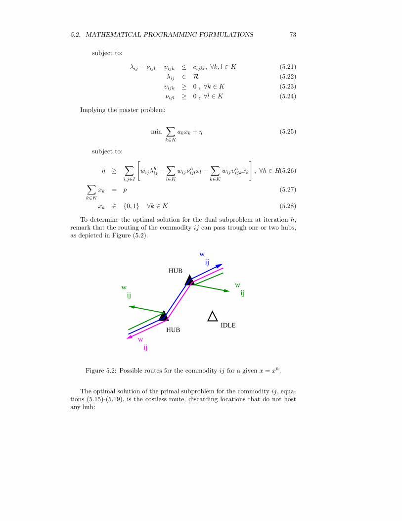
5.2. MATHEMATICAL PROGRAMMING FORMULATIONS 73
subject to:
λij − νijl − υijk ≤ cijkl , ∀k, l ∈ K (5.21)
λij ∈ R (5.22)
υijk ≥ 0 , ∀k ∈ K (5.23)
νijl ≥ 0 , ∀l ∈ K (5.24)
Implying the master problem:
min∑
k∈K
akxk + η (5.25)
subject to:
η ≥∑
i,j∈I
[
wijλhij −
∑
l∈K
wijνhijlxl −
∑
k∈K
wijυhijkxk
]
, ∀h ∈ H(5.26)
∑
k∈K
xk = p (5.27)
xk ∈ 0, 1 ∀k ∈ K (5.28)
To determine the optimal solution for the dual subproblem at iteration h,remark that the routing of the commodity ij can pass trough one or two hubs,as depicted in Figure (5.2).
w ij
w ij
IDLE
HUB
HUB
w ij
w ij
Figure 5.2: Possible routes for the commodity ij for a given x = xh.
The optimal solution of the primal subproblem for the commodity ij, equa-tions (5.15)-(5.19), is the costless route, discarding locations that do not hostany hub:

74CHAPTER 5. INTEGRATING FACILITY LOCATION AND NETWORK DESIGN
wij · min(k,l)
cijkl|yhk = yh
l = 1
(5.29)
The dual variables computation with economical interpretation (meaningfulvalues) is a clue for an efficient implementation. Here, λij is the highest possibleprice difference between i and j and υijk and νijl are additional taxes paid toroute the flow ij trough hubs k and l. Using the complementary slackness, theoptimal dual solution for commodity ij is given by:
λhij = min(k,l)
cijkl|yhk = yh
l = 1
(5.30)
υhijk = 0, if yh
k = 1 (5.31)
υhijk = max
0, maxl
λhij − cijkl
, if yhk = 0 (5.32)
νhijl = 0, if yh
l = 1 (5.33)
νhijl = max
0, maxk
λhij − cijkl
, if yhl = 0 (5.34)
To adapt our decomposition scheme to the Uncapacitated Hub Location Prob-lem, we must observe that the master problem does not have information aboutthe flow constraints. To determine only feasible solutions when decomposing theUncapacitated Hub Location Problem it is necessary to add a single constraint inx to the master problem ensuring the installation of at least one hub, replacingthe fixed number of hubs to locate by a maximum number of possible hubs:
min∑
k∈K
akxk + η (5.35)
subject to:
η ≥∑
i,j∈I
[
wijλhij −
∑
l∈K
wijνhijlxl −
∑
k∈K
wijυhijkxk
]
, ∀h ∈ H(5.36)
∑
k∈K
xk ≤ |K| (5.37)
∑
k∈K
xk ≥ 1 (5.38)
xk ∈ 0, 1 ∀k ∈ K (5.39)
5.2.1 Improving the Design of the Local Access Network
The former hub-and-spoke formulations deal with the client-server interconnec-tion cost in a very simple way. This is not interesting in some applications wherethe major costs are just in the local access network. In fact, traditional hub-and-spoke models optimize the client-server assignment while solving a quadratic

5.2. MATHEMATICAL PROGRAMMING FORMULATIONS 75
location model. However, to improve the treatment of the local access networkalso dealing with the client-hub assignment it is not easy. Our idea here is todetach the two network levels, optimizing the local access network and solvingthe associated quadratic location problem in a separated way.
It is natural to suppose that the city/state/country under study is dividedin a set of regions. This kind of partitioning, as suggested by Figure (5.3), canbe induced by a series of different factors like ground occupation policy, popula-tional density, geographical interference and other social, politic and economiccriteria. The installation of at least a server per region in ensured and natural.Inside each region, there exists a set of candidate locations to host the server,that are interconnected each other and to the final customers by a potentiallocal access network. The role of the server is to deal with the local access de-mands an concentrate all the traffic, correctly addressing it to the other regionsin the city/state/country.
We define Ik ⊂ I as the set of all candidate sites for the location of server k.To implement this partitioning scheme, we define a binary matrix P that haspki = 1 if the site i can host the server k and pki = 0, otherwise.
To overcome the local access network design problem, let us consider firstthe graph G = (V, E) that represents the potential local access network for agiven region, as suggested in Figure (5.3). We are making the assumption thateach region is self-contained, what means that we are not considering the arcsof the potential local access network that interconnect one region to another Ifinside this particular region we have |Ik| candidate sites to host a server, thelocal access network design problem with congestion costs will be solved |Ik |times, each one considering a different candidate site i ∈ Ik as the origin offlow. This task will be performed with the aid of the methods and algorithmstreated in chapter 4. Since this is not expensive, and also can be carried outusing parallel computing, we will assume that can be done in reasonable time.
Now, given all the optimal local access network design costs, for each servercandidate location, we will use them to define a linear server installation costmatrix A = (aki). This matrix has as many lines as servers and as many columnsas the sum of all the candidate sites of all servers, having the same dimensionsof P . The integration of the two levels of design is ensured by the incorporationof the local access network costs into aki.
We are now capable to adapt our models and algorithms for QAP to work onthis problem. Modifying equations (2.20)-(2.23) for our network design/facilitylocation model, we remember that there are some candidate sites for a facility,but only one possible facility for each location. We can now re-write the QAPmodel as:
min∑
k∈K
∑
i∈Ik
akixki +∑
(i,j)∈E
∑
k∈K,l∈K,k 6=l
cijfklij (5.40)
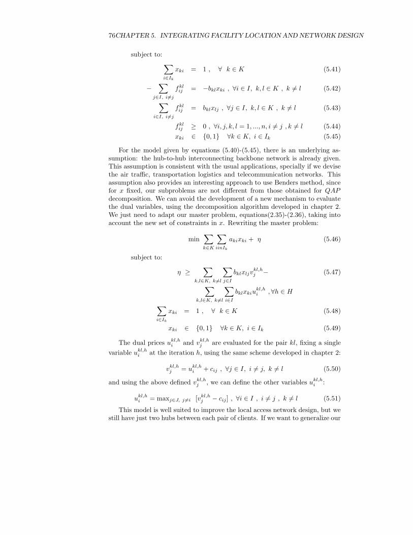
76CHAPTER 5. INTEGRATING FACILITY LOCATION AND NETWORK DESIGN
subject to:
∑
i∈Ik
xki = 1 , ∀ k ∈ K (5.41)
−∑
j∈I, i6=j
fklij = −bklxki , ∀i ∈ I, k, l ∈ K , k 6= l (5.42)
∑
i∈I, i6=j
fklij = bklxlj , ∀j ∈ I, k, l ∈ K , k 6= l (5.43)
fklij ≥ 0 , ∀i, j, k, l = 1, ..., n, i 6= j , k 6= l (5.44)
xki ∈ 0, 1 ∀k ∈ K, i ∈ Ik (5.45)
For the model given by equations (5.40)-(5.45), there is an underlying as-sumption: the hub-to-hub interconnecting backbone network is already given.This assumption is consistent with the usual applications, specially if we devisethe air traffic, transportation logistics and telecommunication networks. Thisassumption also provides an interesting approach to use Benders method, sincefor x fixed, our subproblems are not different from those obtained for QAPdecomposition. We can avoid the development of a new mechanism to evaluatethe dual variables, using the decomposition algorithm developed in chapter 2.We just need to adapt our master problem, equations(2.35)-(2.36), taking intoaccount the new set of constraints in x. Rewriting the master problem:
min∑
k∈K
∑
iinIk
akixki + η (5.46)
subject to:
η ≥∑
k,l∈K, k 6=l
∑
j∈I
bklxljvkl,hj − (5.47)
∑
k,l∈K, k 6=l
∑
i∈I
bklxkiukl,hi , ∀h ∈ H
∑
i∈Ik
xki = 1 , ∀ k ∈ K (5.48)
xki ∈ 0, 1 ∀k ∈ K, i ∈ Ik (5.49)
The dual prices ukl,hi and vkl,h
j are evaluated for the pair kl, fixing a single
variable ukl,hi at the iteration h, using the same scheme developed in chapter 2:
vkl,hj = ukl,h
i + cij , ∀j ∈ I, i 6= j, k 6= l (5.50)
and using the above defined vkl,hj , we can define the other variables ukl,h
i :
ukl,hi = maxj∈J, j 6=i [vkl,h
j − cij ] , ∀i ∈ I , i 6= j , k 6= l (5.51)
This model is well suited to improve the local access network design, but westill have just two hubs between each pair of clients. If we want to generalize our

5.2. MATHEMATICAL PROGRAMMING FORMULATIONS 77
model, we must obtain scale-economies when designing this system, sometimesusing alternative routes to address flow for a given origin-destination pair. Thisfeature can be accomplished if we rewrite the above formulation, in such a waythat becomes possible to route flows trough more than two hubs.
5.2.2 Generalized Model Including Hub Transshipment
and Network Design
The first logical step to generalize our network design location model is to enabletransshipment between servers. Transshipment can be particularly interesting ifwe set up congestion costs between hubs. Rewriting constraints (5.42) and (5.43)as a single transshipment constraint, we can overcome the task. It is necessaryto remark that in this case we will not observe trivial solutions when writingQAP with a transshipment constraint [77], since each facility is constrained toits own region:
min∑
k∈K
∑
i∈Ik
akixki +∑
i∈I
∑
j∈I
∑
k∈K
∑
l∈K
γdijfklij (5.52)
subject to:
∑
j∈I
fklji −
∑
j∈I
fklij = bklxlipli − bklxkipki , ∀i ∈ I, k, l ∈ K (5.53)
∑
i∈Ik
xki = 1 , ∀k ∈ K (5.54)
fklij ≥ 0 , ∀i, j ∈ I, k, l ∈ K (5.55)
xki ∈ 0, 1 , ∀k ∈ K, i ∈ Ik (5.56)
The key for the above formulation is the set of constraints (5.53), that usesthe matrix P to create conditions for nodes and arcs outside regions k and l tobe used for transshipment of the commodity kl. Here, the matrix D is a distancematrix established between all the candidate sites of all regions, and γ is a costper unit flow per distance for transportation. From our experience on QAP , wecan see that one set of assignment constraints is not necessary, since a serverof a given region can not be located outside this region. We must observe alsothat this formulation (that includes transshipment) is derived from the originalKoopmans and Beckmann formulation for QAP , and has o(n2m2)+o(n2)+o(n)variables and o(nm2) + o(n) constraints. We remark that local access networkcontributes with the majority of the cost. Since the existence of linear costsmakes QAP more suitable to solve, once defined the server locations all thatremains is a multicommodity minimum cost flow problem.
If it is necessary to design the backbone, we can add network design at theupper level. Introducing the variables yij that decide the installation of the arcij, it is possible to rewrite Equations (5.52)-(5.56) as:
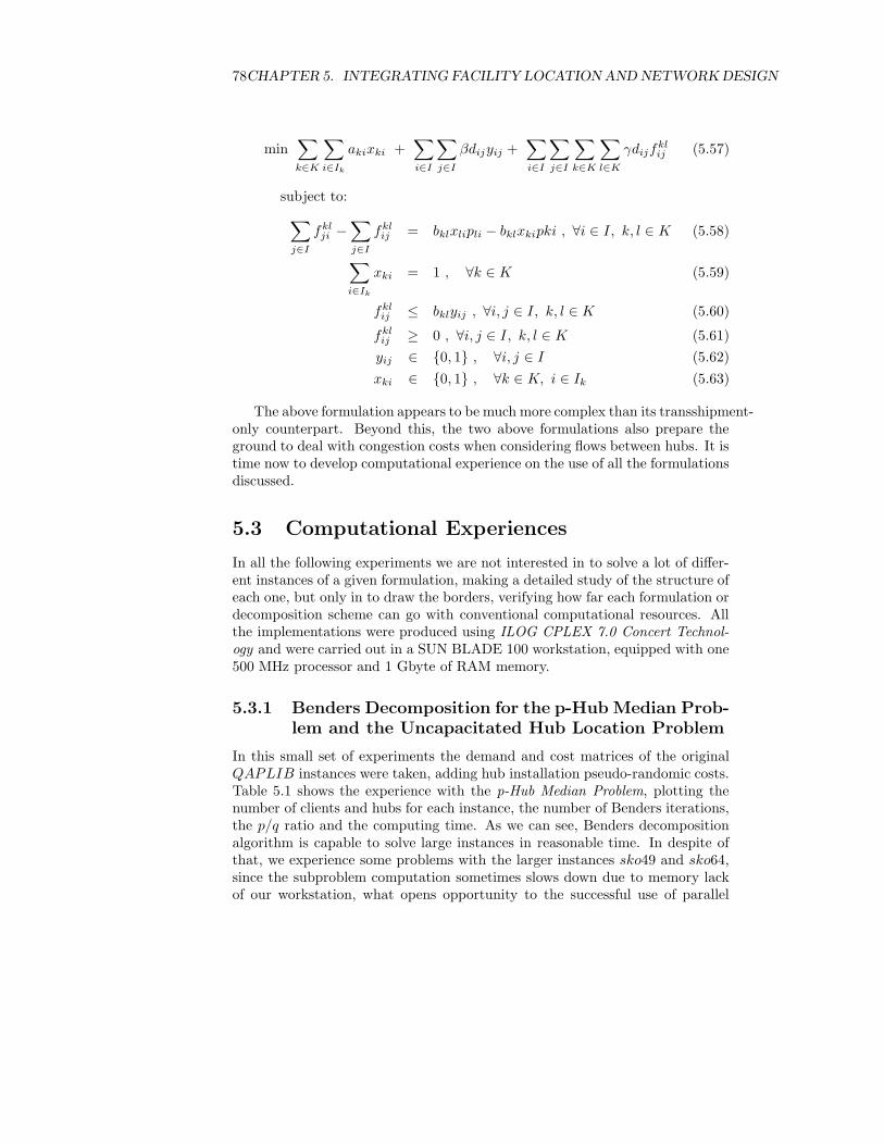
78CHAPTER 5. INTEGRATING FACILITY LOCATION AND NETWORK DESIGN
min∑
k∈K
∑
i∈Ik
akixki +∑
i∈I
∑
j∈I
βdijyij +∑
i∈I
∑
j∈I
∑
k∈K
∑
l∈K
γdijfklij (5.57)
subject to:
∑
j∈I
fklji −
∑
j∈I
fklij = bklxlipli − bklxkipki , ∀i ∈ I, k, l ∈ K (5.58)
∑
i∈Ik
xki = 1 , ∀k ∈ K (5.59)
fklij ≤ bklyij , ∀i, j ∈ I, k, l ∈ K (5.60)
fklij ≥ 0 , ∀i, j ∈ I, k, l ∈ K (5.61)
yij ∈ 0, 1 , ∀i, j ∈ I (5.62)
xki ∈ 0, 1 , ∀k ∈ K, i ∈ Ik (5.63)
The above formulation appears to be much more complex than its transshipment-only counterpart. Beyond this, the two above formulations also prepare theground to deal with congestion costs when considering flows between hubs. It istime now to develop computational experience on the use of all the formulationsdiscussed.
5.3 Computational Experiences
In all the following experiments we are not interested in to solve a lot of differ-ent instances of a given formulation, making a detailed study of the structure ofeach one, but only in to draw the borders, verifying how far each formulation ordecomposition scheme can go with conventional computational resources. Allthe implementations were produced using ILOG CPLEX 7.0 Concert Technol-ogy and were carried out in a SUN BLADE 100 workstation, equipped with one500 MHz processor and 1 Gbyte of RAM memory.
5.3.1 Benders Decomposition for the p-Hub Median Prob-
lem and the Uncapacitated Hub Location Problem
In this small set of experiments the demand and cost matrices of the originalQAPLIB instances were taken, adding hub installation pseudo-randomic costs.Table 5.1 shows the experience with the p-Hub Median Problem, plotting thenumber of clients and hubs for each instance, the number of Benders iterations,the p/q ratio and the computing time. As we can see, Benders decompositionalgorithm is capable to solve large instances in reasonable time. In despite ofthat, we experience some problems with the larger instances sko49 and sko64,since the subproblem computation sometimes slows down due to memory lackof our workstation, what opens opportunity to the successful use of parallel

5.3. COMPUTATIONAL EXPERIENCES 79
Original Number of Number of Number of Benders p/qinstance clients hubs flow variables iterations cost ratio Time[s]
nug7 7 2 2058 8 0.000 0nug7 2 4 0.252 0nug7 2 3 0.504 0nug7 2 3 0.756 0nug7 5 3 6.784 0nug12 12 1 19008 6 0.009 0nug12 2 6 0.102 0nug12 2 4 0.306 0nug12 3 26 0.000 3nug12 3 5 0.172 0nug12 3 4 0.343 0nug12 3 3 0.515 0nug12 3 3 0.859 0nug12 4 22 0.000 2nug12 4 3 0.317 0nug12 4 3 0.951 0nug12 4 3 1.585 0nug12 6 3 5.862 1nug15 15 3 47250 72 0.000 24nug15 3 12 0.108 1nug15 3 8 0.137 0nug15 3 7 0.205 0nug15 4 7 0.285 1nug15 4 5 0.358 0nug15 5 6 0.396 0nug15 6 3 0.511 0nug20 20 1 152000 9 0.067 1nug20 3 8 0.123 1nug20 4 9 0.220 0nug20 5 13 0.088 1nug20 5 9 0.175 1nug20 5 8 0.263 0nug20 5 7 0.312 1nug20 5 7 0.312 0nug20 6 6 0.406 1nug20 7 3 0.544 0nug30 30 3 783000 105 0.013 93nug30 3 53 0.027 25nug30 4 45 0.047 19nug30 4 30 0.071 10nug30 5 24 0.093 8ste36a 36 2 1632960 54 0.034 43sko49 49 6 5647152 133 0.053 482sko49 6 38 0.107 75sko64 64 6 16515072 72 3.340 408
Table 5.1: Benders decomposition for the p-Hub Median Problem.
computing. In Table 5.2 we have the experiments with the Uncapacitated HubLocation Problem, showing the same parameters emphasized in Table 5.1.
We believe that rewrite these classical hub-and-spoke models as flow formu-lations was decisive when considering the performance of the Benders algorithm.We also believe that these flow formulations can be enhanced, granting the so-lution of very large instances with the aid of parallel computing.

80CHAPTER 5. INTEGRATING FACILITY LOCATION AND NETWORK DESIGN
Original Number of Number of Number of Benders p/qinstance clients hubs flow variables iterations cost ratio Time [s]had12 12 8 19008 14 0.219 1had14 14 8 35672 5 0.089 0had14 8 3 0.148 1had16 16 12 61440 9 0.051 0had16 12 7 0.062 0had16 12 6 0.071 0had16 12 4 0.109 0had18 18 12 99144 7 0.056 1had18 12 7 0.058 0nug7 7 1 2058 5 0.165 2nug7 2 6 0.252 0nug7 3 6 0.252 1nug7 4 6 0.252 1nug7 7 7 0.277 0nug12 12 2 19008 7 0.102 0nug12 6 8 0.172 1nug12 7 12 0.190 1nug12 8 8 0.172 1nug12 9 8 0.172 0nug12 10 7 0.053 0nug12 10 6 0.071 1nug12 10 5 0.080 0nug12 10 5 0.106 0nug12 10 11 0.136 1nug12 10 3 0.150 0nug12 10 9 0.205 0nug12 10 15 0.399 0nug15 15 6 47250 8 0.216 1nug15 7 6 0.066 0nug15 7 6 0.070 0nug15 10 8 0.062 1nug15 10 6 0.079 0nug15 10 6 0.083 0nug15 10 23 0.188 2nug15 10 33 0.296 2nug15 10 3 0.413 0nug30 30 6 783000 6 0.089 2nug30 6 5 0.118 2nug30 6 11 0.227 3nug30 6 7 0.325 2nug30 10 8 0.101 2nug30 10 8 0.118 2nug30 10 6 0.130 1nug30 10 12 0.358 4nug30 10 14 0.399 4nug30 10 12 0.432 3sko49 49 6 5647152 14 0.250 26sko49 10 14 0.250 26sko49 30 112 0.000 341sko49 30 9 0.169 16sko49 30 8 0.187 14sko49 30 13 0.267 24sko49 30 5 0.312 8sko49 49 14 0.165 25sko49 49 13 0.202 24sko64 64 49 16515072 4 0.396 18sko64 49 3 0.792 11ste36a 36 10 1632960 15 0.437 8ste36a 18 9 0.483 5ste36a 18 9 0.640 4ste36a 18 9 0.644 5
Table 5.2: Benders decomposition for the Uncapacitated Hub Location Problem.

5.3. COMPUTATIONAL EXPERIENCES 81
5.3.2 The Integrated Model: QAP + Local Access Net-
work Design With Congestion Costs
We report now our experiences with the integrated model, described in section5.2.1. The solution of the integrated model must be made in two phases: firstevaluating the local access costs as suggested in chapter 4, and then, embeddingthe local access costs on the aki coefficients, solving the model given by equations(5.40)-(5.45) in his decomposed form. The solved instances are purely pseudo-randomic, do not sustaining the triangular inequality, and are represented bynames beginning with net plus the size of K and the size of I . They wereproduced in a realistic way, ensuring that costs to install infrastructure arealways equal or superior to operational costs, with the aid of a generator writtenin C++ and compiled with GNU GCC 3.0.
Table 5.3 shows the number of severs (hubs), the total number of possible lo-cations and consequently the number of flow variables, the number of iterationsof Benders algorithm, the p/q cost ratio and the computing times.
Problem Number of Possible Number of Benders p/qname servers locations flow variables iterations cost ratio Time[s]net624 6 24 17424 7 1.711 0net824 8 24 32448 30 2.537 3net1030 10 30 81300 161 1.361 137net1030 10 30 81300 4 7.843 0net1236 12 36 171504 7 8.061 1net1248 12 48 304704 3 1.835 1net1260 12 60 475920 26 1.582 6net1260 12 60 475920 3 15.820 1net1560 15 60 756900 70 1.668 33net2060 20 60 1369200 14 2.490 5net20100 20 100 3802000 114 2.423 181net20100 20 100 3802000 15 4.847 23net20100 20 100 3802000 3 121.166 2net30150 30 150 19579500 54 4.685 391net40200 40 200 62408000 85 5.316 2177
Table 5.3: Computational results for the integrated model.
As we can see, the computational experiments have been quite limited, butthe Benders decomposition scheme is able to obtain solutions for very largeinstances. Since the growing of the flow variables is really explosive in thisformulation, limiting the size of problems that are solvable inside the computermain memory, parallel computing is a reasonable alternative to the solution oflarger instances.
5.3.3 Testing the Hub Transshipment Network Design Model
The instances solved here are also purely pseudo-randomic. These randomicinstances do not sustain the triangular inequality, and are represented by namesbeginning with rnet plus the size of K and the size of I . They were producedin a realistic way, ensuring that costs to install infrastructure (servers and arcsinterconnecting them) are always superior to operational costs.

82CHAPTER 5. INTEGRATING FACILITY LOCATION AND NETWORK DESIGN
In Table 5.4, we show the obtained results for the experience with model(5.57)-(5.63). This table shows the numbers of variables (integer and continu-ous), the quality of the linear programming bound and the solution time. Table5.4 shows that the linear programming relaxation is very strong. This can beexplained by two reasons: the location problem uses linear installation costs,what induces indivisible locations (see chapter 2), and for a fixed server loca-tion, what remains is a multicommodity network design problem, having anextremely strong formulation (see [116]). On the other hand, the linear pro-grams generated by this location/network design model are very hard to solve,what explains the large computing times. It was also not possible to solve prob-lems beyond 15 severs and 45 candidate sites, since CPLEX always crashesdown due to lack of memory beyond these values. This fact suggests that theuse of Benders decomposition for this problem is straightforward and must addsolution power, if well developed.
problem Number of Variables Bound Install. Network Costs Optimal Computingname Integer Continuous Quality Cost (ND + OC) Cost Time[s]
net624.dat 24 20736 0.954 369 17821 18190 6net824.dat 24 36864 0.977 3744 33207 37113 12net824.dat 0.955 468 33369 33837 9net1030.dat 0.959 457 55648 56105 46net1030.dat 0.997 27609 61438 89047 36net1030.dat 30 90000 1 218970 80183 326153 19net1030.dat 0.941 175176 106171 379747 200net1030.dat 0.926 175176 98798 345974 108net1030.dat 0.992 109485 90017 252002 644net1030.dat 0.987 109485 81485 229970 42net1030.dat 0.96 109485 80183 216668 28net1030.dat 0.963 31968 65460 117828 882net1030.dat 0.914 29438 62433 105771 97net1030.dat 0.98 27609 61503 91352 45net1030.dat 0.912 27609 61114 89047 37net1236.dat 36 186624 0.965 252768 165929 563697 20760net1236.dat 0.929 242112 146485 451597 2967net1236.dat 0.961 235088 137776 403464 109net1236.dat 0.925 227632 130608 359054 36net1236.dat 0.945 35994 110298 146292 265net1236.dat 0.969 753 94189 94942 537net1248.dat 48 331776 0.917 71392 81069 152461 70net1545.dat 45 455625 0.993 44949 100938 145887 292
Table 5.4: Report for a brief experiment using the Hub Transshipment NetworkDesign model.
5.4 Concluding Remarks
The obtained results concerning location/network design problems with inter-dependence on the location of serves are very expressive. Future improvementsof the Benders decomposition algorithms of this chapter will make possible tosolve very larger instances at reasonable time, if we use parallel computing,specially on the field of interacting hub facilities systems design.
The task of integration of the models of local access network design andfacility location with interdependency, using a QAP framework, was well ac-

5.4. CONCLUDING REMARKS 83
complished. The produced flow formulation can handle with large instances atreasonable cost.
Our Benders decomposition algorithms are robust enough to deal with largescale hard to solve mixed integer programming problems, designing very com-plex systems.
It is always important to remember that our local access network is capac-itated in this case, computing congestion costs, what ensures the quality ofservice maintenance for the final customer.
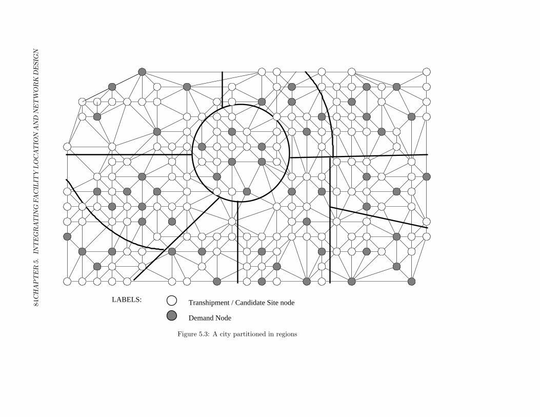
84C
HA
PT
ER
5.
INT
EG
RAT
ING
FA
CIL
ITY
LO
CAT
ION
AN
DN
ET
WO
RK
DE
SIG
N
LABELS: Transhipment / Candidate Site node
Demand Node
Figure 5.3: A city partitioned in regions

5.4
.C
ON
CLU
DIN
GR
EM
AR
KS
85
LABELS: Transhipment / Candidate Site node
Server−to−Server Network
Client−Server Network
Server
Demand Node
Figure 5.4: A feasible solution

86CHAPTER 5. INTEGRATING FACILITY LOCATION AND NETWORK DESIGN

Chapter 6
Conclusions and Future
Work
6.1 Contributions
6.1.1 The Quadratic Assignment Problem
On the cases where we can define or compute heterogeneous profitabilities, it ispossible to solve large instances of QAP , without an excessive computationalcost or the use of massive parallel computing. This conclusion has its founda-tions on the pioneer work of Koopmans and Beckmann and also on the workof Heffley, many years later. The inclusion of heterogeneous profits for locationis a natural step when considering location theory, and can introduce externalenvironment influence on the location decision process.
Once established this, the new flow formulation has proved to unify desirablequalities for a good mathematical programming implementation: be easy tosolve and to grant good linear programming bounds. These two qualities aredirectly responsible for the good computing times achieved, and also for thesolution of large instances at reasonable cost, until now obtainable only troughthe use of computational grids.
For the instances of size beyond 40, the Benders decomposition algorithmappears to be a good choice to find an exact solution, avoiding excessive spaceand time complexity, if we observe some conditions about the cost structure, asmentioned in chapter 2.
The new flow formulation and the associated Benders decomposition schemeare original contributions of this work. There is no solution report for instancesof QAP from n = 30 to 64, without the aid of computational grids, even forp/q > 0. The current literature of this problem do not address p/q 6= 0, loosingthe QAP application framework.
87

88 CHAPTER 6. CONCLUSIONS AND FUTURE WORK
6.1.2 The Placement of Electronics With Thermal Effects
As a subproduct of the solution of large QAP instances, we could derive a per-formance guarantee heuristic for the electronics placement with thermal effects.
The approach of the specific literature for this problem is with the aid ofmeta-heuristics, as Genetic Algorithms and Simulated Annealing. This factmakes the performance guarantee heuristic presented in chapter 3 another orig-inal contribution of this work.
It is interesting to point that other quantities — depending on the selectedapplication — could be used as secondary quality criteria for the solution. Also,depending on other design parameters, a lot of other kinds of information couldbe considered for this particular problem. For instance, the maximal temper-ature over an electronics board or the minimal dispersion of heavy industrialatmospheric residues.
6.1.3 The Local Access Network Design With Congestion
Costs
We have also presented a multi-commodity flow formulation for the local ac-cess network design problem with congestion costs. We have studied an exactmethod to solve the problem, based on generalized Benders decomposition. Wehave also confirmed the possibility of exactly solving such problems with freesoftware mathematical programming packages, and for this purpose we have asurprisingly good alternative to commercial softwares.
Yet the computational experiments have been limited in chapter 4, our expe-rience suggests that a certain number of these modeling and solution strategiescan be applied to the frequently occurring problems where the congestion costcomponent is important. Our conclusion is that generalized Benders decompo-sition emerges as a good method, since it is enough robust to deal with mixedinteger nonlinear programs. The relevance of this type of model is now increas-ing because emerging Internet services requires larger bandwidth in the localaccess network and also because applications concerning multi-party multicast-ing tree construction should take into account congestion costs.
Once established the importance of the congestion costs, the solution of thegenerated nonlinear mixed-integer programs is already an original contributionof this work.
6.1.4 Integrating Facility Location and Network Design
The obtained results concerning location/network design problems with inter-dependence on the location of serves are very expressive, as pointed in chapter5. Future improvements of the Benders decomposition algorithms of chapter 5will make possible to solve very large instances at reasonable time, if we useparallel computing, specially on the field of interacting hub facilities systemsdesign.

6.2. HINTS FOR FUTURE WORK 89
The task of integration of the models of local access network design andfacility location with interdependency, using a QAP framework, was well ac-complished. The produced flow formulation can handle with large instances atreasonable cost.
Our Benders decomposition algorithms are robust enough to deal with largescale hard to solve mixed integer programming problems, designing very com-plex systems.
It is always important to remember that our local access network is capac-itated in this case, computing congestion costs, what ensures the quality ofservice maintenance for the final customer.
6.2 Hints for Future Work
We are about to obtain expressive results concerning location/network designproblems with interdependency on the location of facilities. The future develop-ment of a Benders decomposition algorithm of this problem will make possibleto solve large instances at reasonable computational cost.
It is also important to remember that our local access network is capacitated,and on the solution of network design at this level, we are computing congestioncosts, ensuring the quality of service maintenance for the final customer.
For future work, when considering QAP , it is necessary to better explore theequilibrium between bound quality and cost of computation, detecting when andhow to merge easy to compute and stronger and hard to compute formulationsfor a given problem.
In the field of QAP applications, it can be noted that a lot of real lifeproblems can be viewed as instances of quadratic assignment problems andthat it is sometimes possible to propose other quality criteria for the solution.Nowadays, this kind of solution is valuable, since the environmental impact ofany kind of large scale human implementation has becoming more important. Itis desirable to have the lower transport cost for intermediate commodities in thedesign of a regional industrial complex, and to take into account the dispersionof heavy industrial atmospheric residues. There is no doubt that air quality isa great part of quality of life, and that environmental concerns must be in thetop of the list of all modern industrial management. One could still deal withthe noise level of machinery on the low plant lay-out design.
About local access network design, another question for investigation is thegeneration of approximate solutions by heuristics with the objective of addingcuts to the Benders master problem in a preprocessing phase (in the currentimplementation our preprocessing phase only includes the solution of a shortestpath problem and a minimal spanning tree problem). These new cuts mightreduce the total number of Benders cycles, but the necessary time to solve eachmaster problem might be increased since the master problem would have moreconstraints. The trade off between these two aspects should be better evaluated.
Concerning the formulations and decomposition schemes presented in chap-ter 5, additional computational experience is necessary. The investigation of

90 CHAPTER 6. CONCLUSIONS AND FUTURE WORK
the cost trade offs for hub-and spoke systems is very important and must adda comprehensive picture of this complex kind of system. It is also interestingto compare the monolithic implementation of traditional hub-and-spoke modelsand the decomposed versions. The development of a well suited decompositionscheme for the Hub Transshipment Network Design model can add solutionpower, making possible to solve large instances.

Bibliography
[1] H.P. Adams and T. Johnson. Improved linear programming bounds for thequadratic assignment problem. DIMACS Series in Discrete Mathematicsand Theoretical Computer Science, 16:43–77, 1994.
[2] C.H. Aikens. Facility location models for distribution planning. EuropeanJournal of Operations Research, 22:263–279, 1985.
[3] Y.P. Aneja. An integer linear programming approach to Steiner problemin graphs. Networks, 10:167–178, 1980.
[4] K.M. Anstreicher. Eigenvalue bounds versus semidefinite relaxationsfor the quadratic assignment problem. SIAM Journal of Optimization,11:254–265, 2001.
[5] K.M. Anstreicher and N.W. Brixius. A new bound for the quadratic as-signment problem based on convex quadratic programming. MathematicalProgramming Series A, 89:341–357, 2001.
[6] K.M. Anstreicher, N.W. Brixius, J.P. Goux, and J. Linderoth. Solvinglarge quadratic assignment problems on computational grids. Mathemat-ical Programming Series B, 91:563–588, 2001.
[7] T. Aykin. On the location of hub facilities. Transportation Science,22:155–157, 1988.
[8] T. Aykin. A quadratic integer program for the location of interacting hubfacilities. European Journal of Operations Research, 46:409–411, 1990.
[9] T. Aykin. Lagrangian relaxation based approaches to capacitated hub-and-spoke network design problem. European Journal of Operational Re-search, 79:501–523, 1994.
[10] E. Balas and C. Bergthaller. Benders method revisited. Journal of Com-putational and Applied Mathematics, 9(1):3–12, 1983.
[11] E. Ballas and M.J. Saltzman. An algorithm for the tree-index assignmentproblem. Operations Research, 39:150–161, 1991.
91

92 BIBLIOGRAPHY
[12] A. I. Barvinok. Computational complexity of orbits in representations ofsymmetric groups. Adv. Soviet. Math., 9:161–182, 1992.
[13] M.S. Bazaraa and H.D. Sherali. Benders partitioning scheme applied toa new formulation of the quadratic assignment problem. Naval ResearchLogistics Quarterly, 12:29–41, 1980.
[14] J.E. Beasley. An algorithm for solving large capacitated warehouse lo-cation problems. European Journal of Operations Research, 33:314–325,1988.
[15] J.E. Beasley. An sst-based algorithm for the Steiner problem in graphs.Networks, 19:1–16, 1989.
[16] A. Bejan, G. Tsatsaronis, and M. Moran. Thermal Design and Optimiza-tion. Interscience, 1st edition, 1995.
[17] J. F. Benders. Partitioning procedures for solving mixed integer variablesprogramming problems. Numerische Methematik, 4:238–252, 1962.
[18] R.T. Berger, C.R. Coullard, and M.S. Daskin. Modeling and solving lo-cation routing problems with route-length constraints. TransportationScience, 1996.
[19] O. Berman, D.I. Ingco, and A.R. Odoni. Improving the location of min-isum facilities through network modification. The Annals of OperationsResearch, 40:1–16, 1992.
[20] G. Birkhoff. Tres observaciones sobre el algebra lineal. Rev Univ. Nac.Tucuman, A(5):147–151, 1946.
[21] R.R. Boorstyn and H. Frank. Large-scale network topological optimiza-tion. IEEE Transactions on Communications, COM-25:29–47, 1977.
[22] D.S. Boyalakuntla and J.Y. Murthy. Hierarquical compact models forsimulation of electronic chip packages. IEEE Transactions on Componentsand Packaging Technologies, 25(4):629–634, 2002.
[23] R. E. Burkard. Discrete Location Theory: Locations with spatial inter-actions: the quadratic assignment problem, volume 1. Wiley and Sons, 1edition, 1991.
[24] R.E. Burkard. Selected topics on assignment problems. Technical Report175, Techinshe Universitat Graz, Austria, November 1999.
[25] R.E. Burkard and E. Cela. Heuristics for biquadratic assignment problemand their computational comparison. European Journal of OperationsResearch, 83:283–300, 1995.
[26] R.E.. Burkard and E. Cela. The quadratic assignment problem: theoryand algorithms. Kluwer Academic Publishers, 1(1), 1998.
BIBLIOGRAPHY 93
[27] R.E. Burkard and E. Cela. Linear assignment problems and extensions.Handbook of Combinatorial optimization, 4(1):221–300, 1999.
[28] R.E. Burkard, E. Cela, P. Pardalos, and L.S. PItsoulis. The quadraticassignment problem. Handbook of Combinatorial optimization, 3(1):241–339, 1998.
[29] R.E. Burkard, S. Karisch, and F. Rendl. QAPLIB - A quadratic assign-ment problem library. European Journal of Operations Research, 17:115–119, 1991.
[30] P. Burmann, A. Raman, and S.V. Garimella. Dynamics and topologyoptimization for piezoeletric fans. IEEE Transactions on Componentsand Packaging Technologies, 25(4):592–600, 2002.
[31] J. F. Campbell, G. Stiehr, A. T. Ernst, and M. Krishnamoorthy. Solvinghub arc location problems on a cluster of workstations. Parallel Comput-ing, 29:555–574, 2003.
[32] J.F. Campbell. Continuous and discrete demand hub location problems.Transportation Research B, 27B(6):473–482, 1993.
[33] J.F. Campbell. Integer programming formulations of discrete hub locationproblems. European Journal of Operations Research, 72:387–405, 1994.
[34] J.F. Campbell. A survey of network hub location. Studies in LocationalAnalysis, 6:31–49, 1994.
[35] M. Chandy and K. M. Rusell. The design of multipoint linkages ina teleprocessing tree network. IEEE Transactions on Communications,COM-21:1062–1066, 1972.
[36] N. Christofides and J.E. Beasley. Extensions to a lagrangean relaxationapproach for the capacitated warehouse location problem. European Jour-nal of Operations Research, 12:19–28, 1983.
[37] R. Church and C. ReVelle. The maximal covering location problem. Re-gional Science Association Papers, 32:101–118, 1974.
[38] A. Claus and N. Maculan. Une nouvelle formulation du probeme de Steinersur un graphe. Technical Report 280, Centre de Recherche sur les Trans-ports, Universite de Montreal, Canada, 1983.
[39] K.J. Craig, D.J. Kock, and P. Gauche. Minimization of heat sink massusinf CFD and mathematical optimization. Journal of Electronics Manu-facturing, 121(3):143–147, 1999.
[40] G. Dantzig. Linear Programming and Extensions. Princeton UniversityPress, 1962.

94 BIBLIOGRAPHY
[41] Z. Drezner and G.O. Wesolowsky. Network design: Selection and designof links and facility location. Transportation Research Part A, 37:241–256,2003.
[42] R.P.M. Ferreira and H. P. L. Luna. Discrete capacity and flow assign-ment algorithms with performance guarantee. Computer Communica-tions, 26:1056–1069, May 2003.
[43] G. Finke, R.E.. Burkard, and F. Rendl. Quadratic assignment problems.Annals of Discrete Mathematics, 31:61–82, 1987.
[44] L.R. Ford and D.R. Fulkerson. Maximal flow through a network. CanadianJournal of Mathematics, 8:399–404, 1956.
[45] P.M. Franca and H.P.L. Luna. Solving stochastic transportation-locationproblems by generalized Benders decomposition. Transportation Science,16:113–126, 1982.
[46] A.M. Frieze and L. Yadegar. On the quadratic assignment problem. Dis-crete Applied Mathematics, 5:89–98, 1983.
[47] B. Gavish. Topological design of centralized computer networks - formu-lations and algorithms. Networks, 12:355–377, 1982.
[48] B. Gavish. Formulations and algorithms for the capacitated minimal di-rected tree. Journal of the ACM, 30:118–132, 1983.
[49] B. Gavish. Augmented Lagrangean based algorithms for centralized net-work design. IEEE Transactions on Communications, COM-33:1247–1257, 1985.
[50] B. Gavish. Topological design of telecommunication networks - Localaccess design methods. Annals of Operations Research, 33:17–71, 1991.
[51] A. M. Geoffrion. Generalized Benders decomposition. Journal of Opti-mization Theory And Applications, 10:237–260, 1972.
[52] A.M. Geoffrion. Generalized Benders decomposition. Journal of Opti-mization Theory and Applications, 10(4):237–260, 1972.
[53] A.M. Geoffrion and G.W. Graves. Multicomodity distribution systemdesign by Benders decomposition. Management Science, 20:822–844, 1974.
[54] M. Gerla and L. Kleinrock. On the topological design of distributed com-puter networks. IEEE Transactions on Communications, 25:48–60, 1977.
[55] M. X. Goemans and Y.-S. Mying. A catalogue of Steiner tree formulations.Networks, 23:19–28, 1993.
[56] M. C. Goldstein. Design of long-distance telecommunication networks -the Telepak problem. IEEE Transactions on Circuit Theory, CT-20:186–192, 1973.

BIBLIOGRAPHY 95
[57] L. Gouveia. A comparison of directed formulations for the capacitatedminimal spanning tree problem. Telecommunication Systems, 1:51–76,1993.
[58] K.S.S. Gupta and P.K. Srimani. Core-based tree with forwarding regions(cbt-fr); a protocol for reliable multicasting in ad hoc networks. Journalof Parallel and Distributes Computing, 61:1249–1277, 2001.
[59] P. Hahn and T. Grant. Lower bounds for the quadratic assignment prob-lem based upon a dual formulation. Operations Research, 46(6):912–922,1998.
[60] S.L. Hakimi. Optimum location of switching centers and the absolutecenters and medians of a graph. Operations Research, 12:450–459, 1964.
[61] D.R. Heffley. The quadratic assignment problem: A note. Econometrica,40(6):1155–1163, 1972.
[62] J. Hellstrand, T. Larsson, and A. Migdalas. A characterization of the unca-pacitated network design polytope. Operations Research Letters, 12:159–163, 1992.
[63] D.S. Hochbaum and A. Segev. Analysis of a flow problem with fixedcharges. Networks, 19:291–312, 1989.
[64] Y.J. Huang and S.L. Fu. Thermal placement design for mcm applications.Journal of Electronic Packaging, 122(2):115–120, 2000.
[65] Y.J. Huang, S.L. Fu, S.L. Jen, and M.H. Guo. Fuzzy thermal modelingfor mcm placement. Microelectronics Journal, 32(10):836–868, 2001.
[66] Y.J. Huang, M.H. Guo, and S.L. Fu. Reliability and routability consider-ation for mcm placement. Microelectronics Reliability, 42(1):83–91, 2002.
[67] F. K. Hwang and D. S. Richards. Steiner tree problems. Networks, 22:55–89, 1992.
[68] F. K. Hwang, D.S. Richards, and P. Winter. The Steiner Tree Problem.North-Holland, 1992.
[69] P. J. Juell, D. Brekke, and R. Vetter. A multicast tree constructionsalgorithm for large multiparty conferences. Telecommunication Systems,17:299–321, 2001.
[70] M. Junger and V. Kaibel. On the SAQP polytope. SIAM Journal ofOptimization, 11:444–463, 2000.
[71] M. Junger and V. Kaibel. Box-inequalities for quadratic assignment poly-topes. Math. program. Ser. A, 91:175–197, 2001.

96 BIBLIOGRAPHY
[72] D. Katanyutaveetip. Real-time optimal multicast routing. ComputerCommunications, 2002. Article in Press.
[73] L. Kaufman and F. Broeckx. An algorithm for the quadratic assignmentproblem using Benders decomposition. European Journal of OperationsResearch, 2:204–211, 1978.
[74] J.G. Klincewicz. Hub location in backbone/tributary network design: areview. Location Science, 6:307–335, 1998.
[75] T. Koch and A. Martin. Solving Steiner tree problems in graphs to opti-mality. Networks, 32:207–232, 1998.
[76] D. Konig. Graphok es matrixok. Mat. Fiz. Lapok, 38:116–119, 1931.
[77] T.C. Koopmans and M. Beckmann. Assignment problems and the locationof economic activities. Econometrica, 25:53–76, 1957.
[78] A.A. Kuehn and M.J. Hamburger. A heuristic program for locating ware-houses. Management Science, 9:643–666, 1963.
[79] H. W. Kuhn. The hungarian method for the assignment problem. NavalResearch Logistics Quarterly, 2:83–98, 1955.
[80] E.L. Lawler. The quadratic assignment problem. Management Science,9:586–599, 1963.
[81] S. Lorente, W. Wechsatol, and A. Bejan. Optimization of tree shapedflow distribution structures over a disc disc-shaped area. Int. Journal ofEnergy Research, 27(8):715–723, 2003.
[82] A. Losch. The Economics of Location. New Haven, 1 edition, 1954. Trans-lated from German edition 1944.
[83] A. Lucena and J. E. Beasley. A branch and cut algorithm for the Steinerproblem in graphs. Networks, 31:39–59, 1998.
[84] H. P. L. Luna and P. Mahey. Bounds for global optimization of capacityexpansion and flow assignment problems. Operations Research Letters,26:211–216, 2000.
[85] H.P.L. Luna, N. Ziviani, and R.M.B. Cabral. The telephonic switchingcentre network problem: Formalization and computational experience.Discrete Applied Mathematics, 18:199–210, 1987.
[86] N. Maculan. A new linear programming formulation for the shortest s-directed spanning tree problem. Journal of Combinatorics, Information& Systems Sciences, 11:53–56, 1986.
[87] N. Maculan. The Steiner problem in graphs. Annals of Discrete Mathe-matics, 31:185–212, 1987.

BIBLIOGRAPHY 97
[88] N. Maculan, D. Arpin, and S. Nguyen. Le probleme de Steiner sur ungraphe oriente: Formulations et relaxations. Matematica Aplicada e Com-putacional, 7:109–118, 1988.
[89] T. L. Magnanti and R. T. Wong. Accelerating Benders decomposition: Al-gorithmic enhancement and model selection criteria. Operations Research,29(3):464–483, 1981.
[90] T.L. Magnanti, P. Mirchandani, and R.T. Wong. Tailoring Benders de-composition for uncapacitated network design. Mathematical Program-ming Study, 26:112–154, 1986.
[91] A. Makhorin. GLPK - The GNU linear programming kit. TechnicalReport 1, Moskow Aviation Institute, Moscow, Russia, 2001. available inhttp://www.gnu.org/glpk.
[92] G.R. Mateus and H.P.L Luna. Decentralized decision-making and capaci-tated facility location. The Annals of Regional Science, 26:361–377, 1992.
[93] G.R. Mateus, H.P.L. Luna, and A.B. Sirihal. Heuristics for distributionnetwork design in telecommunication. Journal of Heuristics, 6(SpecialNumber on Telecommunications):131–148, 2000.
[94] G.R. Mateus and J.M. Thizy. Exact sequential choices of locations in anetwork. Annals of Operations Research, 86:199–219, 1999.
[95] K. Mehlhorn. A faster approximation algorithm for the Steiner problemin graphs. Information Processing Letters, 27:125–128, 1988.
[96] S. Melkote and M.S. Daskin. Capacitated facility location/network designproblems. European Journal of Operations Research, 129:481–495, 2001.
[97] S. Melkote and M.S. Daskin. An integrated model of facility location andtransportation network design. Trasportation Research Part A, 35:515–538, 2001.
[98] E.S. Mills. The efficiency of spatial competition. The Regional ScienceAssociation Papers, 25:71–82, 1970.
[99] T.S. Motzkin. The assignment problem. In Proceedings of Symposia inApplied Mathematics, Numerical Analysis. McGraw-Hill, 1956.
[100] E.Y.K. Ng, C.P. Tso, Z.M. Wen, and K.F. Choo. Numerical simulation offlow and conjugate heat transfer in a microchannel for electronics cooling.Journal of Electronics Manufacturing, 9(2):141–153, 1999.
[101] M. O’Kelly. The location of interacting hub facilities. TransportationScience, 20:92–106, 1986.

98 BIBLIOGRAPHY
[102] M. O’Kelly. A quadratic integer program for the location of interact-ing hub facilities. European Journal of Operational Research, 32:393–404,1986.
[103] M. O’Kelly, D. Bryan, , D. Skorin-Kapov, and J. Skorin-Kapov. Hubnetwork design and multiple allocation: A computational study. LocationScience, 4:125–138, 1986.
[104] M. O’Kelly and M.W. Horner. Embedding economies of scale concepts forhub network design. Journal of Transport Geography, 9:255–265, 2001.
[105] M. O’Kelly and H.L. Miller. The hub network design problem. Journalof Transport Geography, 2(1):31–40, 1994.
[106] M.W. Padberg and M.P. Rijal. Loacation, Scheduling, Design and IntegerProgramming. Kluwer Academic Publishers, Boston, 1 edition, 1996.
[107] P. Pardalos, F. Rendl, and H. Wolkowickz. The quadratic assignmentproblem: a survey of recent developments. DIMACS Series on DiscreteMathematics and Computer Science, 16:1–42, 1994.
[108] S.V. Patankar. Numerical Heat Transfer and Fluid Flow. HemispherePublishing Corporation, 1st. edition, 1980.
[109] H. Pirkul and J. Current. The hierarquical network design problemwith transshipment facilities. European Journal of Operational Research,52:338–347, 1991.
[110] H. Pirkul and D.A. Schiling. An efficient procedure for designing singleallocation hub and spoke systems. Management Science, 44:235–242, 1998.
[111] N.V. Queipo, R. Devarakonda, and J.A.C. Humphrey. Genetic algorithmsfor thermosciences research - application to the optimized cooling of elec-tronic components. Int. Journal of Heat and Mass Transfer, 37(6):893–908, 1994.
[112] N.V. Queipo and G.F. Gil. Multiobjective optimal placement of con-vectively cooled electronic components on printed wiring boards. IEEETransactions on Components Packaging and Manufacturing Technology,21(1):142–153, 1998.
[113] N.V. Queipo and G.F. Gil. Multiobjective optimal placement of convec-tively and condutively cooled electronic components on printed wiringboards. Journal of Electronic Packaging, 122(2):152–159, 2000.
[114] M. Queiroz and C. Humes. The projected pairwise multicommodity flowpolyhedron. Applied Mathematics Letters, 14(4):443–448, May 2001.
[115] K.G. Ramakrishnan, M.G.C. Resende, B. Ramachandran, and J.F. Penky.Tight QAP Bounds Via Linear Programming. World Scientific PublishingCo., Singapore, 1 edition, 2002.

BIBLIOGRAPHY 99
[116] C.D. Randazzo and H.P.L. Luna. A comparison of optimal methods forlocal access uncapacitated network design. The Annals of Operations Re-search, 106:263–286, 2001.
[117] L.A.O. Rocha, S. Lorente, and A. Bejan. Constructal design for cooling adisc-shaped area by conduction. Int. Journal of Heat and Mass Transfer,45(8):1643–1652, 2002.
[118] J.L. Rosales, A. Ortega, and J.A.C. Humphrey. A numerical simulation ofthe convective heat transfer in confined channel flow past square cylinders:comparison of inline and offset tandem pairs. Int. Journal of Heat andMass Transfer, 44(3):587–603, 2001.
[119] B. Rothfarb and M. C. Goldstein. The one-terminal Telepak problem.Operations Research, 19:156–169, 1971.
[120] S. Sahni and T. Gonzalez. P-complete approximation problems. Journalof Association of Computing Machinery, 23:555–565, 1976.
[121] P.A. Samuelsom. Spatial price equilibrium and linear programming.American Economic Review, 42:284–303, 1952.
[122] L. Schwiebert and R. Chintalapati. Improved fault recovery for core basedtrees. Computer Communications, 23:816–824, 2000.
[123] D.S. Steinberg. Cooling Techniques for Electronic Equipment. Inter-science, 2nd edition, 1991.
[124] C. Toregas, R. Swain, C. ReVelle, and L. Bergmann. The location ofemergency service facilities. Operations Research, 19:1363–1373, 1971.
[125] P.G Tucker. Models aid the analisys of electronics cooling. Microwavesand RF, 40(6):95–96, 2001.
[126] J.A. Visser and Kock D.J. Optimization of heat sink mass using theDYNAMIC-Q numerical optimization. Communications in NumericalMethods in Engineering, 18(10):721–727, 2002.
[127] W. Wechsatol, S. Lorente, and A. Bejan. Optimal tree-shaped networksfor fluid flow in a disc disc-shaped body. Int. Journal of Heat and MassTransfer, 45(25):4911–4924, 2002.
[128] P. Winter. Steiner problem in networks: a survey. Networks, 17:129–167,1987.
[129] R.T. Wong. A dual ascent algorithm for the Steiner problem in directedgraphs. Mathematical Programming, 28:271–287, 1984.
[130] G. Zapfel and M. wasner. Planning and optimization of hub-and-spoketransportations networks of cooperative third-party logistics providers.International Journal of Production Economics, 78:207–220, 2002.
100 BIBLIOGRAPHY
[131] Z.J. Zuo, L.R. Hoover, and A.L. Phillips. Advanced thermal architeturefor cooling of high power electronics. IEEE Transactions on Componentsand Packaging Technologies, 25(4):629–634, 2002.


