19
Factor Analysis Advanced Financial Accounting II Åbo Akademi School of Business
| Date post: | 06-Sep-2018 |
| Category: |
Documents |
| Upload: | truongtuyen |
| View: | 220 times |
| Download: | 0 times |

Factor Analysis
Advanced Financial Accounting II
Åbo Akademi School of Business

Factor analysis
A statistical method used to describe variability among observed variables in terms of fewer unobserved variables called factors
The observed variables are modeled as linear combinations of the factors plus error terms
The information gained about the interdependen-cies can be used later to reduce the set of variables in a dataset
Related to principal component analysis (PCA) PCA performs a variance-maximizing rotation of the variable
space, i.e. takes into account all variability in the variables
Factor analysis estimates how much of the variability is due to common factors
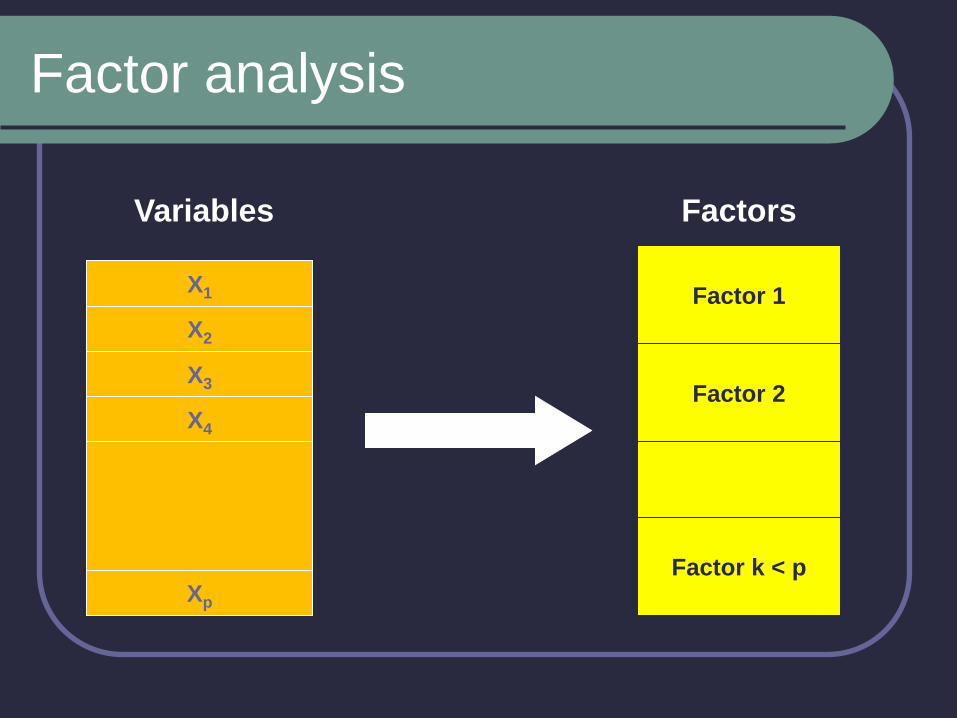
Factor analysis
X1
X2
X3
X4
Xp
Variables
Factor 1
Factor 2
Factor k < p
Factors

Factor analysis - an example:
Financial ratios
DSales
DAssets
EBIT-%
ROI
CR
Variables
Growth
Profitability
Solidity
Factors
ROE
CF/Sales
Equity Ratio
QR

Types/purposes of factor analysis
Exploratory factor analysis Used to uncover the underlying structure of a
relatively large set of variables
A priori assumption is that any indicator may be associated with any factor
No prior theory, factor loadings are used to intuit the factor structure of the data
Confirmatory factor analysis Seeks to determine if the number of factors and the
loadings of the measured variables on them confirm to what is expected on the basis of a pre-established theory

Factor analysis with SPSS
Analyze
⇒ Dimension Reduction
⇒ Factor
Extraction method, several alternatives e.g. Principal Components (the most common)
Maximum Likelihood
Number of factors Statistically defined (based on eigenvalues)
Used defined (Fixed) when prior assumption on factor structure
Rotation in order to extract a clearer factor pattern, several alternatives, e.g. Varimax
Oblimin

Confirmatory Factor analysis - an example:
Financial Ratios for Finnish listed companies
9 variables
DSales, DAssets, EBIT-%, ROI, ROE, Cash
Flow(Operations)/Sales, Equity Ratio, Quick Ratio
Current Ratio
Fixed number of factors: 3
Predefined assumption on three factors: Growth,
Profitability and Solidity
Extraction method: Principal Components
Analysis
Rotation method: Varimax
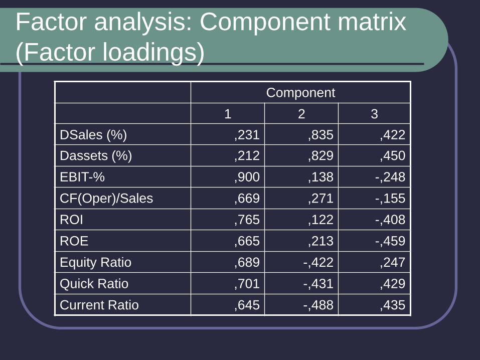
Factor analysis: Component matrix
(Factor loadings)
Component
1 2 3
DSales (%) ,231 ,835 ,422
Dassets (%) ,212 ,829 ,450
EBIT-% ,900 ,138 -,248
CF(Oper)/Sales ,669 ,271 -,155
ROI ,765 ,122 -,408
ROE ,665 ,213 -,459
Equity Ratio ,689 -,422 ,247
Quick Ratio ,701 -,431 ,429
Current Ratio ,645 -,488 ,435
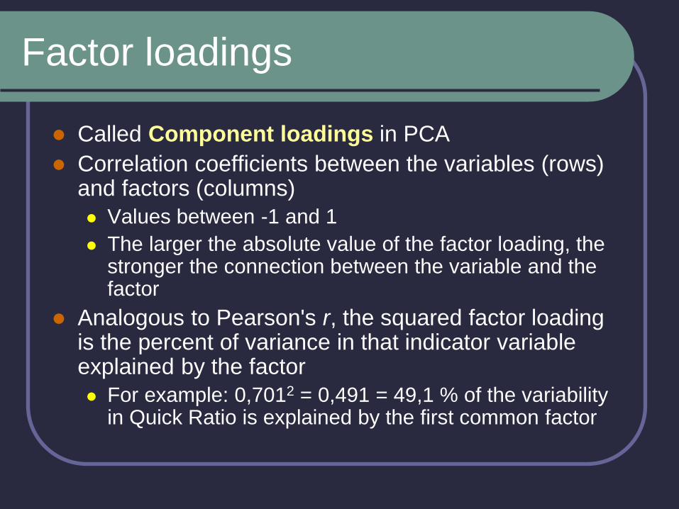
Factor loadings
Called Component loadings in PCA
Correlation coefficients between the variables (rows) and factors (columns)
Values between -1 and 1
The larger the absolute value of the factor loading, the stronger the connection between the variable and the factor
Analogous to Pearson's r, the squared factor loading is the percent of variance in that indicator variable explained by the factor
For example: 0,7012 = 0,491 = 49,1 % of the variability in Quick Ratio is explained by the first common factor

Interpreting the factor loadings and
rotating the loadings matrix
A common problem in interpreting the unrotated factor loadings matrix is that all the most significant loadings are concentrated in one or two first factors
One way to obtain more interpretable results is to rotate the solution
The most common rotation method is Varimax rotation
An orthogonal rotation (Rotated factors uncorrelated)
Maximizes the variance of the squared loadings of a factor on all the variables in the matrix
Each factor will tend to have either large or small loadings of any particular variable
Yields results that make it as easy as possible to identify each variable with a single factor

Factor analysis: Varimax-rotated
component matrix
Component
1 2 3
DSales (%) ,132 -,055 ,953
DAssets (%) ,100 -,048 ,960
EBIT-% ,869 ,344 ,128
CF(Oper)/Sales ,671 ,183 ,248
ROI ,875 ,177 ,003
ROE ,834 ,037 ,031
Equity Ratio ,274 ,795 -,086
Quick Ratio ,173 ,911 ,011
Current Ratio ,111 ,911 -,042

Factor analysis - an example: Financial ratios
for Finnish listed companies
The three pre-assumed factors – Growth, Profitability and Solidity - may be clearly identified in the rotated component matrix
For example Growth is represented by component 3 combining the major part of ratios DSales and DAssets with minor influences from the other seven variables
In the same manner Profitability is represented by component 1 and Solidity by component 2
The component matrix may be further transformed into a Component score coefficient matrix to be used to create new ratios describing the factors

Factor analysis: Communalities
Initial Extraction
DSales (%) 1,000 ,928
DAssets (%) 1,000 ,934
EBIT-% 1,000 ,890
CF(Oper)/Sales 1,000 ,545
ROI 1,000 ,766
ROE 1,000 ,698
Equity Ratio 1,000 ,715
Quick Ratio 1,000 ,861
Current Ratio 1,000 ,843

Communalities
The communalities for a variable are computed by
taking the sum of the squared loadings for that
variable
May be interpreted as multiple R2 values for
regression models predicting the variables of interest
from the factors
The sum of the squared factor loadings for all factors
for a given variable (row) is the variance in that
variable accounted for by all the factors For example 86.1 % of the variation in Quick Ratio is explained by
the three common factors, 13.9 % is left unexplained

Communalities...
One assessment of how well the model is doing can
be obtained from the communalities
Values close to one indicate that the model explains
most of the variation for the variables
Adding up the communality values for individual
variables gives the Total communality of the model
In the example case we have total communality of 7.182
Dividing total communality by the number of variables
gives the percentage of variation explained in the
model
In the example case 7.182/9 = 79.8 %

SPSS: Total Variance Explained
Compo-
nent
Initial Eigenvalues Extraction Sums of Squared
Loadings
Total % of
Variance
Cumulative
%
Total % of
Variance
Cumulative
%
1 3,765 41,832 41,832 3,765 41,832 41,832
2 2,139 23,764 65,595 2,139 23,764 65,595
3 1,277 14,184 79,780 1,277 14,184 79,780
4 ,708 7,871 87,651
... ... ... ...
9 ,103 1,143 100,000
Total variance
explained by the
three factor model
79.78 %
Even an Explorative Factor
Analysis with the default
eigenvalue limit 1,0 in SPSS
would have resulted in extractíng
three factors

Factor analysis: Computing factor
scores
The observed nine ratios for Alma Media 2005 were
DSales - 0.3846
DAssets - 0.2580
EBIT-% 0.1480
Cash Flow(Oper.)/Sales 0.1179
ROI 0.2610
ROE 0.2840
Equity Ratio 0.5201
Quick Ratio 1.7119
Current Ratio 2.9000

Factor analysis: Computing factor scores…
The nine variables may be summarized in three new
variables Profitability, Solidity and Growth by
multiplying the observed ratio values with component
scores:
Profitability = -0.053 × (-0.3846) - 0.071 × (-
0.2580) + 0.314 × 0.1480 + 0.240 × 0.1179 + 0.360
× 0.2610 + 0.374 × 0.2840 - 0.025 × 0.5201- 0.108
× 1.7119 - 0.129 × 2.9000 = -0.129
Solidity = 1.230
Growth = - 0.189
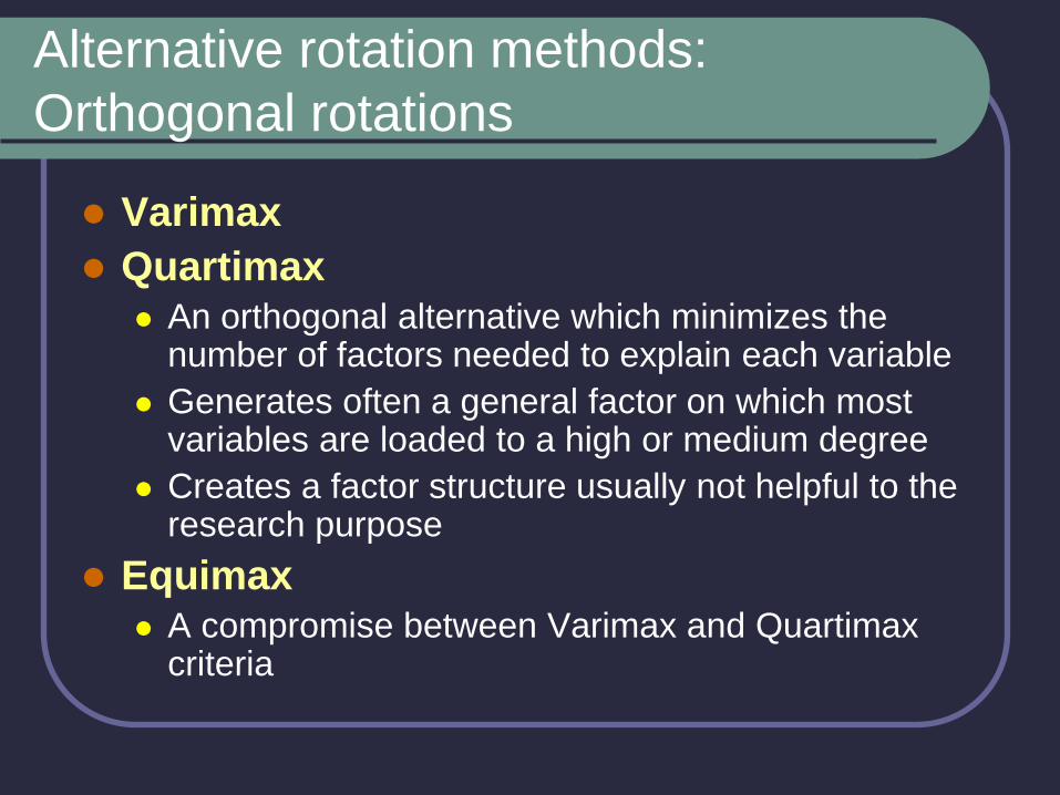
Alternative rotation methods:
Orthogonal rotations
Varimax
Quartimax An orthogonal alternative which minimizes the
number of factors needed to explain each variable
Generates often a general factor on which most variables are loaded to a high or medium degree
Creates a factor structure usually not helpful to the research purpose
Equimax A compromise between Varimax and Quartimax
criteria


