1

Factor Graphs for Quantum ProbabilitiesHans-Andrea Loeliger and Pascal O. Vontobel

Abstract—A factor-graph representation of quantum-mechani-

cal probabilities (involving any number of measurements) is

proposed. Unlike standard statistical models, the proposed rep-

resentation uses auxiliary variables (state variables) that are

not random variables. All joint probability distributions are

marginals of some complex-valued function q, and it is demon-

strated how the basic concepts of quantum mechanics relate to

factorizations and marginals of q.

Index Terms—Quantum mechanics, factor graphs, graphi-

cal models, marginalization, closing-the-box operation, quantum

coding, tensor networks.

I. INTRODUCTION

Factor graphs [2]–[4] and similar graphical notations [5]–[8] are widely used to represent statistical models with manyvariables. Factor graphs have become quite standard in codingtheory [9], but their applications include also communications[10], signal processing [11], [12], combinatorics [13], andmuch more. The graphical notation can be helpful in variousways, including the elucidation of the model itself and thederivation of algorithms for statistical inference.

In this paper, we show how quantum mechanical probabil-ities (including, in particular, joint distributions over severalmeasurements) can be expressed in factor graphs that are fullycompatible with factor graphs of standard statistical modelsand error correcting codes. This is not trivial: despite being astatistical theory, quantum mechanics does not fit into standardstatistical categories and it is not built on the Kolmogorov ax-ioms of probability theory. Existing graphical representationsof quantum mechanics such as Feynman diagrams [14], tensordiagrams [15]–[18], and quantum circuits [19, Chap. 4] do notexplicitly represent probabilities, and they are not compatiblewith “classical” graphical models.

Therefore, this paper is not just about a graphical notation,but it offers a perspective of quantum mechanics that has not(as far as we know) been proposed before.

In order to introduce this perspective, recall that statisticalmodels usually contain auxiliary variables (also called hiddenvariables or state variables), which are essential for factoriz-ing the joint probability distribution. For example, a hiddenMarkov model with primary variables Y1, . . . , Yn

is definedby a joint probability mass function of the form

p(y1, . . . , yn, x0, . . . , xn

) = p(x0)

nY

k=1

p(yk

, xk

|xk�1), (1)

H.-A. Loeliger is with the Department of Information Technology and Elec-trical Engineering, ETH Zurich, Switzerland. Email: loeliger@isi.ee.ethz.ch.

P. O. Vontobel is with the Department of Information Engineering, TheChinese University of Hong Kong. Email: pascal.vontobel@ieee.org.

This paper was presented in part at the 2012 IEEE Int. Symp. on Informa-tion Theory [1].

Copyright (c) 2017 IEEE. Personal use of this material is permitted.However, permission to use this material for any other purposes must beobtained from the IEEE by sending a request to pubs-permissions@ieee.org.

where X0, X1, . . . , Xn

are auxiliary variables (hidden vari-ables) that are essential for the factorization (1). More gen-erally, the joint distribution p(y1, . . . , yn) of some primaryvariables Y1, . . . , Yn

is structured by a factorization of the jointdistribution p(y1, . . . , yn, x0, . . . , xm

) with auxiliary variablesX0, . . . , Xm

and

p(y1, . . . , yn) =X

x0,...,xm

p(y1, . . . , yn, x0, . . . , xm

), (2)

where the sum is over all possible values of X0, . . . , Xm

.(For the sake of exposition, we assume here that all variableshave finite alphabets.) However, quantum-mechanical jointprobabilities cannot, in general, be structured in this way.

We now generalize p(y1, . . . , yn, x0, . . . , xm

) in (2) to anarbitrary complex-valued function q(y1, . . . , yn, x0, . . . , xm

)

such that

p(y1, . . . , yn) =X

x0,...,xm

q(y1, . . . , yn, x0, . . . , xm

). (3)

The purpose of q is still to enable a nice factorization, forwhich there may now be more opportunities. Note that theconcept of marginalization carries over to q; in particular,all marginals of p(y1, . . . , yn) (involving any number ofvariables) are also marginals of q. However, the auxiliaryvariables X0, . . . , Xm

are not, in general, random variables,and marginals of q involving one or several of these variablesare not, in general, probability distributions.

We will show that this generalization allows natural repre-sentations of quantum-mechanical probabilities involving anynumber of measurements. In particular, the factor graphs ofthis paper will represent pertinent factorizations of complex-valued functions q as in (3).

This paper is not concerned with physics, but only with thepeculiar joint probability distributions that arise in quantummechanics. However, we will show how the basic conceptsand terms of quantum mechanics relate to factorizations andmarginals of suitable functions q. For the sake of clarity, wewill restrict ourselves to finite alphabets (with some excep-tions, especially in Appendix B), but this restriction is notessential. Within this limited scope, this paper may even beused as a self-contained introduction to the pertinent conceptsof quantum mechanics.

To the best of our knowlege, describing quantum proba-bilities (and, indeed, any probabilities) by explicitly using afunction q as in (3) is new. Nonetheless, this paper is, ofcourse, related to much previous work in quantum mechanicsand quantum computation. For example, quantum circuits asin [19, Chap. 4] have natural interpretations in terms of factorgraphs as will be demonstrated in Sections V-B and VIII.Our factor graphs are also related to tensor diagrams [15]–[18], [20], see Sections II-B and Appendix A. Also related

2

is the very recent work by Mori [21]. On the other hand,quantum Bayesian networks (see, e.g., [22]) and quantumbelief propagation (see, e.g., [23]) are not immediately relatedto our approach since they are not based on (3) (and they lackProposition 1 in Section II). Finally, we mention that the factorgraphs of this paper are used in [24] for estimating the infor-mation rate of certain quantum channels, and iterative sum-product message passing in such factor graphs is consideredin [25].

The paper is structured as follows. Section II reviews factorgraphs and their connection to linear algebra. In Section III,we express elementary quantum mechanics (with a singleprojection measurement) in factor graphs; we also demonstratehow the Schrodinger picture, the Heisenberg picture, and evenan elementary form of Feynman path integrals are naturallyexpressed in terms of factor graphs. Multiple and more gen-eral measurements are discussed in Section IV. Section Vaddresses partial measurements, decompositions of unitaryoperators (including quantum circuits), and the emergence ofnon-unitary operators from unitary interactions. In Section VI,we revisit measurements and briefly address their realizationin terms of unitary interactions, and in Section VII, wecomment on the origin of randomness. In Section VIII, wefurther illustrate the use of factor graphs by an elementaryintroduction to quantum coding. Section IX concludes themain part of the paper.

In Appendix A, we offer some additional remarks on theprior literature. In Appendix B, we briefly discuss the Wigner–Weyl representation, which leads to an alternative factor-graphrepresentation. In Appendix C, we outline the extension ofMonte Carlo methods to the factor graphs of this paper.

This paper contains many figures of factor graphs thatrepresent some complex function q as in (3). The main figuresare Figs. 14, 25, 38, and 47; in a sense, the whole paper isabout explaining and exploring these four figures.

We will use standard linear algebra notation rather thanthe bra-ket notation of quantum mechanics. The Hermitiantranspose of a complex matrix A will be denoted by AH 4

= AT,where AT is the transpose of A and A is the componentwisecomplex conjugate. An identity matrix will be denoted by I .The symbol “/” denotes equality of functions up to a scalefactor.

II. ON FACTOR GRAPHS

A. BasicsFactor graphs represent factorizations of functions of several

variables. We will use Forney factor graphs1 (also called nor-mal factor graphs) as in [3], [4], [11], where nodes (depictedas boxes) represent factors and edges represent variables. Forexample, assume that some function f(x1, . . . , x5) can bewritten as

f(x1, . . . , x5) = f1(x1, x2, x5)f2(x2, x3)f3(x3, x4, x5). (4)

1Factor graphs as in [2] represent variables not by edges, but by variablenodes. Adapting Proposition 1 for such factor graphs is awkward.

Henceforth in this paper, “factor graph” means “Forney factor graph”; thequalifier “Forney” (or “normal”) will sometimes be added to emphasize thatthe distinction matters.

f1

x1

x2f2

x3f3

x4

x5

Fig. 1. Factor graph (i.e., Forney factor graph) of (4).

X0

Y1

X1

Y2

X2

Y3

X3

Fig. 2. Factor graph of the hidden Markov model (1) for n = 3.

f1

x1

x2f2

x3f3

x4

x5 g

Fig. 3. Closing boxes in factor graphs.

The corresponding factor graph is shown in Fig. 1.In this paper, all variables in factor graphs take values

in finite alphabets (with some exceptions, especially in Ap-pendix B) and all functions take values in C.

The factor graph of the hidden Markov model (1) is shownin Fig. 2. As in this example, variables in factor graphs areoften denoted by capital letters.

The Forney factor-graph notation is intimately connectedwith the idea of opening and closing boxes [4], [11], [26].Consider the dashed boxes in Fig. 3. The exterior function ofsuch a box is defined to be the product of all factors insidethe box, summed over all its internal variables. The exteriorfunction of the inner dashed box in Fig. 3 is

g(x2, x4, x5)4=

X

x3

f2(x2, x3)f3(x3, x4, x5), (5)

and the exterior function of the outer dashed box is

f(x1, x4)4=

X

x2,x3,x5

f(x1, . . . , x5). (6)

The summations in (5) and (6) range over all possible valuesof the corresponding variable(s).

Closing a box means replacing the box with a singlenode that represents the exterior function of the box. Forexample, closing the inner dashed box in Fig. 3 replaces thetwo nodes/factors f2(x2, x3) and f3(x3, x4, x5) by the singlenode/factor (5); closing the outer dashed box in Fig. 3 replacesall nodes/factors in (4) by the single node/factor (6); and

3

pX

g

Fig. 4. Factor graph of E[g(X)] according to (8).

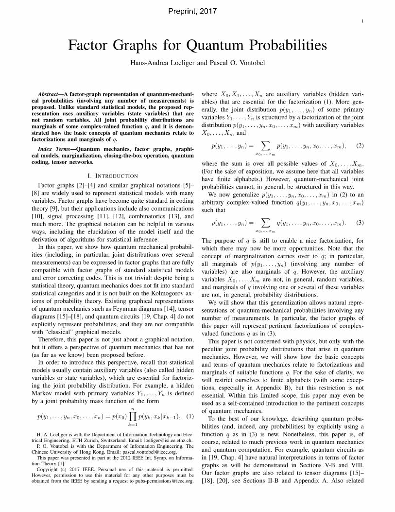
closing first the inner dashed box and then the outer dashedbox replaces all nodes/factors in (4) by

X

x2,x5

f1(x1, x2, x5)g(x2, x4, x5) = f(x1, x4). (7)

Note the equality between (7) and (6), which holds in general:

Proposition 1. Closing an inner box within some outer box(by summing over the internal variables of the inner box) doesnot change the exterior function of the outer box. 2

This simple fact is the pivotal property of Forney factorgraphs. Closing boxes in factor graphs is thus compatiblewith marginalization both of probability mass functions andof complex-valued functions q as in (3), which is the basis ofthe present paper.

Opening a box in a factor graph means the reverse operationof expanding a node/factor into a factor graph of its own.

A half edge in a factor graph is an edge that is connectedto only one node (such as x1 in Fig. 1). The exterior functionof a factor graph2 is defined to be the exterior function ofa box that contains all nodes and all full edges, but all halfedges stick out (such as the outer box in Fig. 3). For example,the exterior function of Fig. 1 is (6). The partition sum3 of afactor graph is the exterior function of a box that contains thewhole factor graph, including all half edges; the partition sumis a constant.

The exterior function of Fig. 2 is p(xn

, y1, . . . , yn), and itspartition sum equals one.

Factor graphs can also express expectations: the partitionsum (and the exterior function) of Fig. 4 is

E[g(X)] =

X

x

p(x)g(x), (8)

where p(x) is a probability mass function and g is an arbitraryreal-valued (or complex-valued) function.

The equality constraint function f= is defined as

f=(x1, . . . , xn

) =

⇢1, if x1 = · · · = x

n

0, otherwise. (9)

The corresponding node (which is denoted by “=”) can serveas a branching point in a factor graph (cf. Figs. 21–24): onlyconfigurations with x1 = . . . = x

n

contribute to the exteriorfunction of any boxes containing these variables.

A variable with a fixed known value will be marked by asolid square as in Figs. 12 and 23.

2What we here call the exterior function of a factor graph, is called partitionfunction in [29]. The term “exterior function” was first used in [30].

3What we call here the partition sum has often been called partitionfunction.

x

A

r y

B

r z

AB

Fig. 5. Factor-graph representation of matrix multiplication (11). The smalldot denotes the variable that indexes the rows of the corresponding matrix.

A

rA

rB

rFig. 6. Factor graph of tr(A) (left) and of tr(AB) = tr(BA) (right).

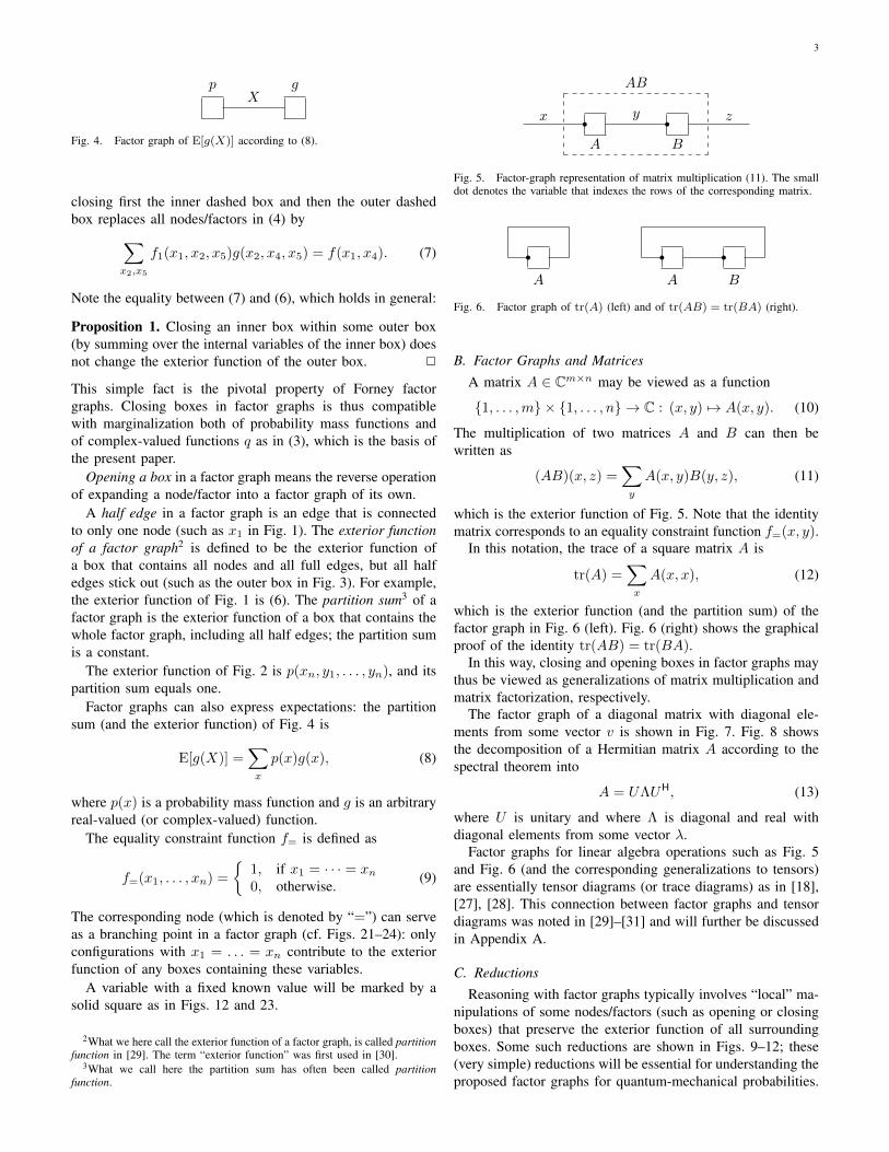
B. Factor Graphs and MatricesA matrix A 2 Cm⇥n may be viewed as a function

{1, . . . ,m}⇥ {1, . . . , n} ! C : (x, y) 7! A(x, y). (10)

The multiplication of two matrices A and B can then bewritten as

(AB)(x, z) =X

y

A(x, y)B(y, z), (11)

which is the exterior function of Fig. 5. Note that the identitymatrix corresponds to an equality constraint function f=(x, y).

In this notation, the trace of a square matrix A is

tr(A) =

X

x

A(x, x), (12)

which is the exterior function (and the partition sum) of thefactor graph in Fig. 6 (left). Fig. 6 (right) shows the graphicalproof of the identity tr(AB) = tr(BA).

In this way, closing and opening boxes in factor graphs maythus be viewed as generalizations of matrix multiplication andmatrix factorization, respectively.

The factor graph of a diagonal matrix with diagonal ele-ments from some vector v is shown in Fig. 7. Fig. 8 showsthe decomposition of a Hermitian matrix A according to thespectral theorem into

A = U⇤UH, (13)

where U is unitary and where ⇤ is diagonal and real withdiagonal elements from some vector �.

Factor graphs for linear algebra operations such as Fig. 5and Fig. 6 (and the corresponding generalizations to tensors)are essentially tensor diagrams (or trace diagrams) as in [18],[27], [28]. This connection between factor graphs and tensordiagrams was noted in [29]–[31] and will further be discussedin Appendix A.

C. ReductionsReasoning with factor graphs typically involves “local” ma-

nipulations of some nodes/factors (such as opening or closingboxes) that preserve the exterior function of all surroundingboxes. Some such reductions are shown in Figs. 9–12; these(very simple) reductions will be essential for understanding theproposed factor graphs for quantum-mechanical probabilities.

4

v

=

Fig. 7. Factor graph of a diagonal matrix with diagonal vector v. The nodelabeled “=” represents the equality constraint function (9).

�=

U

r

UH

r

A

Fig. 8. Factor graph of decomposition (13) according to the spectral theorem.

D. Complex Conjugate PairsA general recipe for constructing complex functions q with

real and nonnegative marginals as in (3) is illustrated inFig. 13, where all factors are complex valued. Note that thelower dashed box in Fig. 13 mirrors the upper dashed box:all factors in the lower box are the complex conjugates of thecorresponding factors in the upper dashed box. The exteriorfunction of the upper dashed box is

g(y1, y2, y3)4=

X

x1,x2

g1(x1, y1)g2(x1, x2, y2)g3(x2, y3) (14)

and the exterior function of the lower dashed box isX

x

01,x

02

g1(x01, y1) g2(x

01, x

02, y2) g3(x

02, y3) = g(y1, y2, y3).

(15)If follows that closing both boxes in Fig. 13 yields

g(y1, y2, y3)g(y1, y2, y3) = |g(y1, y2, y3)|2, (16)

which is real and nonnegative.All factor graphs for quantum-mechanical probabilities that

will be proposed in this paper (except in Appendix B) arespecial cases of this general form. With two parts that arecomplex conjugates of each other, such representations mightseem redundant. Indeed, one of the two parts could certainly bedepicted in some abbreviated form; however, as mathematicalobjects subject to Proposition 1, our factor graphs must containboth parts. (Also, the Monte Carlo methods of Appendix Cwork with samples where x0

k

6= xk

.)

III. ELEMENTARY QUANTUM MECHANICSIN FACTOR GRAPHICS

A. Born’s RuleWe begin with an elementary situation with a single mea-

surement as shown in Fig. 14. In this factor graph, p(x) is

... = =

...

Fig. 9. A two-variable equality constraint (i.e., an identity matrix) can bedropped or addded.

= = =

Fig. 10. A half edge out of an equality constraint node (of any degree) canbe dropped or added.

A�1

r=

A

r = =

Fig. 11. A regular square matrix A multiplied by its inverse reduces to anidentity matrix (i.e., a two-variable equality constraint).

=

x=

x

x

Fig. 12. A fixed known value (depicted as a small solid square) propagatesthrough, and thereby eliminates, an equality constraint.

g

g1X1

g2X2

g3

Y1 Y2 Y3

g

g1

X 01

g2

X 02

g3

Fig. 13. Factor graph with complex factors and nonnegative real marginal(16).

5

p(x)

X=

U

rBH

r

UH

rB

r=

Y

p(y|x)

Fig. 14. Factor graph of an elementary quantum system.

x

U

rBH

rx

UH

rB

r =

Y

Fig. 15. Dashed box of Fig. 14 for fixed X = x. The partition sum of thisfactor graph equals one.

x

U

rBH

r y

x

UH

rB

r y H

Fig. 16. Derivation of (18) and (19).

p(x)

X=

U

rBH

r

UH

rB

r=

Y

⇢ f=

Fig. 17. Regrouping Fig. 14 into a density matrix ⇢ and an equality constraint.

p(x)

X=

U

rBH

r

UH

rB

r=

y

⇢ B(·, y)B(·, y)H

Fig. 18. Fig. 17 for fixed Y = y.

a probability mass function, U and B are complex-valuedunitary M ⇥M matrices, and all variables take values in theset {1, . . . ,M}. The matrix U describes the unitary evolutionof the initial state X . The matrix B defines the basis for theprojection measurement whose outcome is Y (as will furtherbe discussed below). The exterior function of the dashed boxis p(y|x), which we will examine below; with that box closed,the factor graph represents the joint distribution

p(x, y) = p(x)p(y|x). (17)

We next verify that the dashed box in Fig. 14 can indeedrepresent a conditional probability distribution p(y|x). Forfixed X = x, this dashed box turns into (all of) Fig. 15 (seeFig. 12). By the reductions from Figs. 10 and 11, closingthe dashed box in Fig. 15 turns it into an identity matrix. Itfollows that the partition sum of Fig. 15 is I(x, x) = 1 (i.e.,the element in row x and column x of an identity matrix),thus complying with the requirement

Py

p(y|x) = 1.It is then clear from (17) that the partition sum of Fig. 14

equals 1.For fixed X = x and Y = y, the dashed box in Fig. 14

turns into Fig. 16, and p(y|x) is the partition sum of thatfactor graph. The partition sum of the upper part of Fig. 16 isB(·, y)HU(·, x), where U(·, x) is column x of U and B(·, y) iscolumn y of B. The partition sum of the lower part of Fig. 16is U(·, x)HB(·, y). Therefore, the partition sum of Fig. 16 isthe product of these two terms, i.e.,

p(y|x) =��B(·, y)HU(·, x)

��2 (18)

=

��B(·, y)H ��2 , (19)

where 4= U(·, x) is the quantum state (or the wave function).

With a little practice, the auxiliary Figs. 15 and 16 need notactually be drawn and (18) can be directly read off Fig. 14.

B. Density MatrixConsider Figs. 17 and 18, which are regroupings of Fig. 14.

The exterior function of the left-hand dashed box in thesefigures is the density matrix ⇢ of quantum mechanics, whichcan be decomposed into

⇢ =

X

x

p(x)U(·, x)U(·, x)H (20)

(cf. Fig. 8) and which satisfies

tr(⇢) =X

x

p(x) tr�U(·, x)U(·, x)H

�(21)

=

X

x

p(x) tr�U(·, x)HU(·, x)

�(22)

=

X

x

p(x) k(U(·, x)k2 (23)

=

X

x

p(x) (24)

= 1. (25)

The exterior function of the right-hand dashed box in Fig. 17is an identity matrix (i.e., an equality constraint function),as is obvious from the reductions of Figs. 10 and 11. It is

6

p(x)

X=

U

rBH

r

UH

rB

r=

Y

g(y)

p(y)

Fig. 19. Factor graph of expectation (29).

p(x)

X=

U

rBH

r

UH

rB

r=

Y

g(y)

⇢ O

Fig. 20. Factor graph of expectation (30) with general Hermitian matrix O.

then obvious (cf. Fig. 6) that the partition sum of Fig. 17 istr(⇢), which equals 1 by (25). (But we already established inSection III-A that the partition sum of Figs. 14 and 17 is 1.)

The exterior function of the right-hand dashed box in Fig. 18(with fixed Y = y) is the matrix B(·, y)B(·, y)H. From Fig. 14,we know that the partition sum of Fig. 18 is

Px

p(x, y) =

p(y). Using Fig. 6, this partition sum can be expressed as

p(y) = tr

�⇢B(·, y)B(·, y)H

�(26)

= tr

�B(·, y)H⇢B(·, y)

�(27)

= B(·, y)H⇢B(·, y). (28)

Plugging (20) into (28) is, of course, consistent with (18).

C. Observables

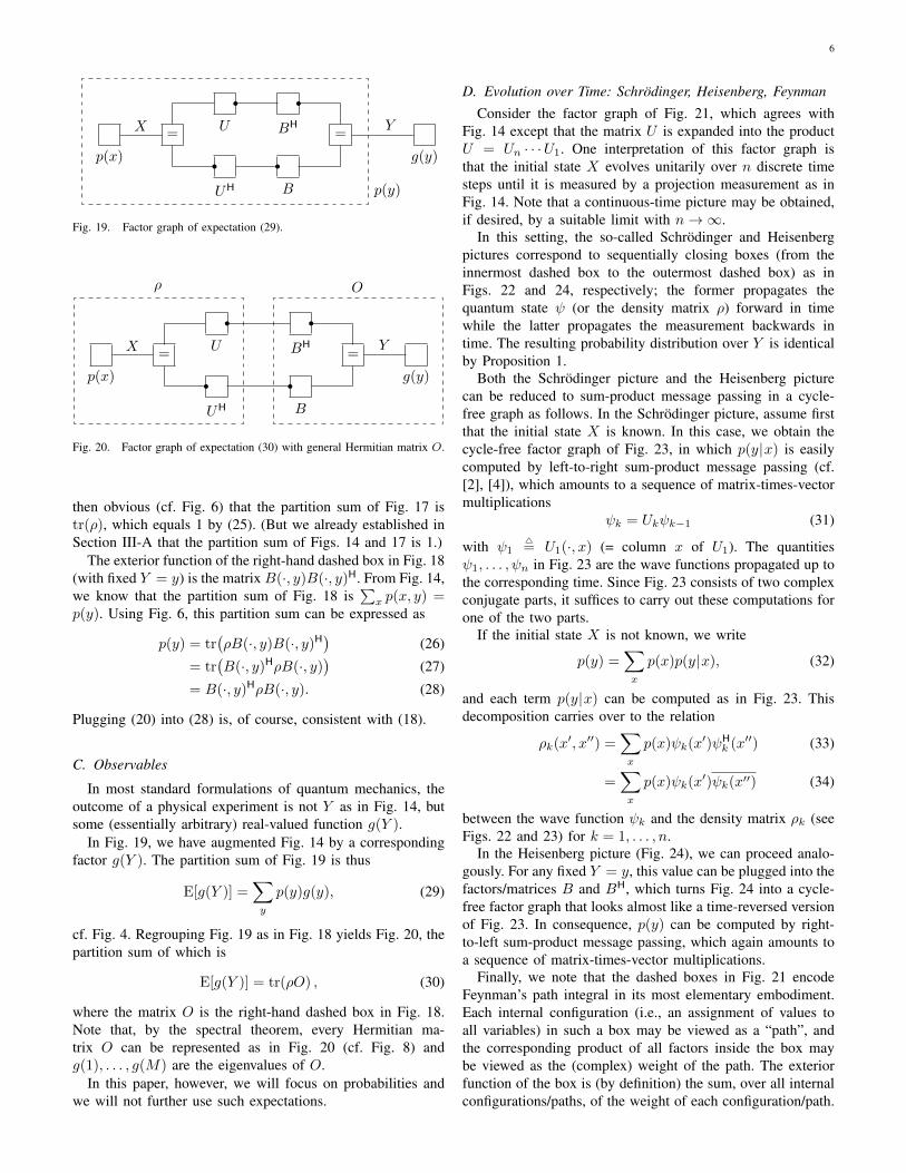
In most standard formulations of quantum mechanics, theoutcome of a physical experiment is not Y as in Fig. 14, butsome (essentially arbitrary) real-valued function g(Y ).

In Fig. 19, we have augmented Fig. 14 by a correspondingfactor g(Y ). The partition sum of Fig. 19 is thus

E[g(Y )] =

X

y

p(y)g(y), (29)

cf. Fig. 4. Regrouping Fig. 19 as in Fig. 18 yields Fig. 20, thepartition sum of which is

E[g(Y )] = tr(⇢O) , (30)

where the matrix O is the right-hand dashed box in Fig. 18.Note that, by the spectral theorem, every Hermitian ma-trix O can be represented as in Fig. 20 (cf. Fig. 8) andg(1), . . . , g(M) are the eigenvalues of O.

In this paper, however, we will focus on probabilities andwe will not further use such expectations.

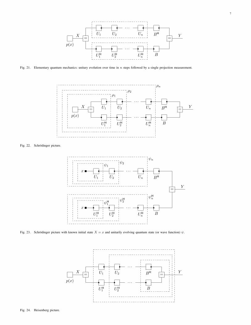
D. Evolution over Time: Schrodinger, Heisenberg, FeynmanConsider the factor graph of Fig. 21, which agrees with

Fig. 14 except that the matrix U is expanded into the productU = U

n

· · ·U1. One interpretation of this factor graph isthat the initial state X evolves unitarily over n discrete timesteps until it is measured by a projection measurement as inFig. 14. Note that a continuous-time picture may be obtained,if desired, by a suitable limit with n ! 1.

In this setting, the so-called Schrodinger and Heisenbergpictures correspond to sequentially closing boxes (from theinnermost dashed box to the outermost dashed box) as inFigs. 22 and 24, respectively; the former propagates thequantum state (or the density matrix ⇢) forward in timewhile the latter propagates the measurement backwards intime. The resulting probability distribution over Y is identicalby Proposition 1.

Both the Schrodinger picture and the Heisenberg picturecan be reduced to sum-product message passing in a cycle-free graph as follows. In the Schrodinger picture, assume firstthat the initial state X is known. In this case, we obtain thecycle-free factor graph of Fig. 23, in which p(y|x) is easilycomputed by left-to-right sum-product message passing (cf.[2], [4]), which amounts to a sequence of matrix-times-vectormultiplications

k

= Uk

k�1 (31)

with 14= U1(·, x) (= column x of U1). The quantities

1, . . . , n

in Fig. 23 are the wave functions propagated up tothe corresponding time. Since Fig. 23 consists of two complexconjugate parts, it suffices to carry out these computations forone of the two parts.

If the initial state X is not known, we write

p(y) =X

x

p(x)p(y|x), (32)

and each term p(y|x) can be computed as in Fig. 23. Thisdecomposition carries over to the relation

⇢k

(x0, x00) =

X

x

p(x) k

(x0) H

k

(x00) (33)

=

X

x

p(x) k

(x0)

k

(x00) (34)

between the wave function k

and the density matrix ⇢k

(seeFigs. 22 and 23) for k = 1, . . . , n.

In the Heisenberg picture (Fig. 24), we can proceed analo-gously. For any fixed Y = y, this value can be plugged into thefactors/matrices B and BH, which turns Fig. 24 into a cycle-free factor graph that looks almost like a time-reversed versionof Fig. 23. In consequence, p(y) can be computed by right-to-left sum-product message passing, which again amounts toa sequence of matrix-times-vector multiplications.

Finally, we note that the dashed boxes in Fig. 21 encodeFeynman’s path integral in its most elementary embodiment.Each internal configuration (i.e., an assignment of values toall variables) in such a box may be viewed as a “path”, andthe corresponding product of all factors inside the box maybe viewed as the (complex) weight of the path. The exteriorfunction of the box is (by definition) the sum, over all internalconfigurations/paths, of the weight of each configuration/path.

7

p(x)

X=

U1

rU2

r . . .

Un

rBH

r

UH1

rUH2

r . . .

UHn

rB

r=

Y

Fig. 21. Elementary quantum mechanics: unitary evolution over time in n steps followed by a single projection measurement.

p(x)

X=

U1

rU2

r . . .

Un

rBH

r

UH1

rUH2

r . . .

UHn

rB

r =

Y

⇢1⇢2

⇢n

Fig. 22. Schrodinger picture.

x

U1

rU2

r . . .

Un

rBH

r 1 2

n

x

UH1

rUH2

r . . .

UHn

rB

r H1

H2

Hn

=

Y

Fig. 23. Schrodinger picture with known initial state X = x and unitarily evolving quantum state (or wave function) .

p(x)

X=

U1

rU2

r . . .

BH

r

UH1

rUH2

r . . .

B

r =

Y

Fig. 24. Heisenberg picture.

8

p(x0)

X0=

U0

r X1

UH0

r X 01

Y1

˜X1

U1

r X2

˜X 01

UH1

r X 02

Y2

˜X2

=

˜X 02

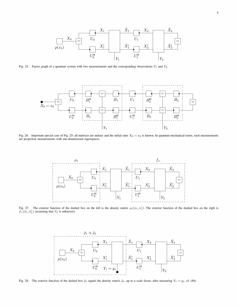
Fig. 25. Factor graph of a quantum system with two measurements and the corresponding observations Y1 and Y2.

X0 = x0

=

U0

rBH

1

r=

B1

rU1

rBH

2

r=

B2

r=

UH0

rB1

r=

Y1

BH1

rUH1

rB2

r=

Y2

BH2

r

Fig. 26. Important special case of Fig. 25: all matrices are unitary and the initial state X0 = x0 is known. In quantum-mechanical terms, such measurementsare projection measurements with one-dimensional eigenspaces.

p(x0)

X0=

U0

r X1

UH0

r X 01

Y1

˜X1

U1

r X2

˜X 01

UH1

r X 02

Y2

˜X2

=

˜X 02

⇢1 f=

Fig. 27. The exterior function of the dashed box on the left is the density matrix ⇢1(x1, x01). The exterior function of the dashed box on the right is

f=(x1, x01) (assuming that Y2 is unknown).

p(x0)

X0=

U0

r X1

UH0

r X 01

Y1 = y1

˜X1

U1

r X2

˜X 01

UH1

r X 02

Y2

˜X2

=

˜X 02

⇢1 / ⇢1

Fig. 28. The exterior function of the dashed box ⇢1 equals the density matrix ⇢1, up to a scale factor, after measuring Y1 = y1, cf. (40).

9

IV. MULTIPLE AND MORE GENERAL MEASUREMENTS

We now turn to multiple and more general measurements.Consider the factor graph of Fig. 25. In this figure, U0 and U1

are M ⇥M unitary matrices, and all variables except Y1 andY2 take values in the set {1, . . . ,M}. The two large boxes inthe figure represent measurements, as will be detailed below.The factor/box p(x0) is a probability mass function over theinitial state X0. We will see that this factor graph (with suitablemodeling of the measurements) represents the joint probabilitymass function p(y1, y2) of a general M -dimensional quantumsystem with two observations Y1 and Y2. The generalizationto more observed variables Y1, Y2, . . . is obvious.

The unitary matrix U0 in Fig. 25 represents the developmentof the system between the initial state and the first mea-surement according to the Schrodinger equation; the unitarymatrix U1 in Fig. 25 represents the development of the systembetween the two measurements.

In the most basic case, the initial state X0 = x0 is knownand the measurements look as shown in Fig. 26, where thematrices B1 and B2 are also unitary (cf. Fig. 14). In this case,the observed variables Y1 and Y2 take values in {1, . . . ,M}as well. Note that the lower part of this factor graph isthe complex-conjugate mirror image of the upper part (as inFig. 13).

In quantum-mechanical terms, measurements as inFig. 26 are projection measurements with one-dimensionaleigenspaces (as in Section III).

A very general form of measurement is shown in Fig. 29.In this case, the range of Y

k

is a finite set Yk

, and for eachyk

2 Yk

, the factor Ak

(xk

, xk

, yk

) corresponds to a complexsquare matrix A

k

(yk

) (with row index xk

and column indexxk

) such thatX

yk2Jk

Ak

(yk

)

HAk

(yk

) = I, (35)

cf. [19, Chap. 2]. A factor-graphic interpretation of (35)is given in Fig. 30. Condition (35) is both necessary andsufficient for Proposition 2 (below) to hold. Measurements asin Fig. 26 are included as a special case with Y

k

= {1, . . . ,M}and

Ak

(yk

) = Ak

(yk

)

H= B

k

(·, yk

)Bk

(·, yk

)

H, (36)

where Bk

(·, yk

) denotes the yk

-th column of Bk

. Note that,for fixed y

k

, (36) is a projection matrix.Measurements will further be discussed in sections V-A

and VI.It is clear from Section II-D that the exterior function of

Fig. 25 (with measurements as in Fig. 26 or as in Fig. 29)is real and nonnegative. We now proceed to analyze thesefactor graphs and to verify that they yield the correct quantum-mechanical probabilities p(y1, y2) for the respective class ofmeasurements. To this end, we need to understand the exteriorfunctions of the dashed boxes in Fig. 27. We begin with thedashed box on the right-hand side of Fig. 27.

Proposition 2 (Don’t Mind the Future). Closing the dashedbox on the right-hand side in Fig. 27 (with a measurement asin Fig. 26 or as in Fig. 29, but with unknown result Y2 of themeasurement) reduces it to an equality constraint function. 2

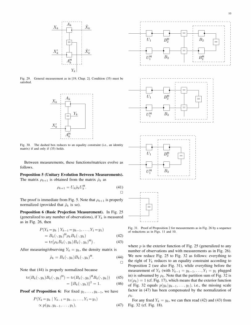
Proof: For measurements as in Fig. 26, the proof amountsto a sequence of reductions according to Figs. 10 and 11, asillustrated in Fig. 31.

For measurements as in Fig. 29, the key step is the reductionof Fig. 30 to an equality constraint, which is equivalent to thecondition (35). ⌅

Proposition 2 guarantees, in particular, that a future mea-surement (with unknown result) does not influence present orpast observations. The proposition clearly holds also for theextension of Fig. 25 to any finite number of measurementsY1, Y2, . . . and can then be applied recursively from right toleft.

We pause here for a moment to emphasize this point: it isobvious from Figs. 25 and 26 (generalized to n measurementsY1, . . . , Yn

) that, in general, a measurement resulting in somevariable Y

k

affects the joint distribution of all other variablesY1, . . . , Yk�1, Yk+1, . . . , Yn

(both past and future) even if theresult Y

k

of the measurement is not known. By Proposition 2,however, the joint distribution of Y1, . . . , Yk�1 is not affectedby the measurement of Y

k

, . . . , Yn

provided that no measure-ment results are known.

Proposition 3 (Proper Normalization). The factor graph ofFig. 25 (with measurements as in Fig. 26 or as in Fig. 29)represents a properly normalized probability mass function,i.e., the exterior function p(y1, y2) is real and nonnegative andP

y1,y2p(y1, y2) = 1. 2

In particular, the partition sum of Fig. 25 equals 1. Again, theproposition clearly holds also for the extension of Fig. 25 toany finite number of measurements Y1, Y2, . . .

Proof of Proposition 3: Apply reductions according toProposition 2 recursively from right to left in Fig. 25, followedby the final reduction

Px0

p(x0) = 1. ⌅Consider now the dashed boxes on the left in Figs. 27

and 28, which correspond to the density matrix before andafter measuring Y1, respectively. A density matrix ⇢ is definedto be properly normalized if

tr(⇢) = 1. (37)

The dashed box left in Fig. 27 is properly normalized(tr(⇢1) = 1) by (25). Proper normalization of ⇢

k

for k > 1

follows from Propositions 5–7 below.Consider next the dashed box in Fig. 28, which we will call

⇢1; it is not a properly normalized density matrix:

Proposition 4 (Trace of the Past).

tr(⇢1) = p(y1); (38)

more generally, with k measurements Y1 = y1, . . . , Yk

= yk

inside the dashed box, we have

tr(⇢k

) = p(y1, . . . , yk). (39)2

The proof is immediate from Propositions 2 and 3 (general-ized to an arbitrary number of measurements). The properlynormalized post-measurement density matrix is then

⇢k

4= ⇢

k

/p(y1, . . . , yk). (40)

10

Xk

Akq ˜X

k

=

Yk

X 0k

AHk

q ˜X 0k

Fig. 29. General measurement as in [19, Chap. 2]. Condition (35) must besatisfied.

Xk

Akq

=

Yk

X 0k

AHk

qFig. 30. The dashed box reduces to an equality constraint (i.e., an identitymatrix) if and only if (35) holds.

Between measurements, these functions/matrices evolve asfollows.

Proposition 5 (Unitary Evolution Between Measurements).

The matrix ⇢k+1 is obtained from the matrix ⇢

k

as

⇢k+1 = U

k

⇢k

UHk

. (41)2

The proof is immediate from Fig. 5. Note that ⇢k+1 is properly

normalized (provided that ⇢k

is so).

Proposition 6 (Basic Projection Measurement). In Fig. 25(generalized to any number of observations), if Y

k

is measuredas in Fig. 26, then

P (Yk

=yk

| Yk�1=y

k�1, . . . , Y1=y1)

= Bk

(·, yk

)

H⇢k

Bk

(·, yk

) (42)= tr

�⇢k

Bk

(·, yk

)Bk

(·, yk

)

H�. (43)

After measuring/observing Yk

= yk

, the density matrix is

⇢k

= Bk

(·, yk

)Bk

(·, yk

)

H. (44)2

Note that (44) is properly normalized because

tr(Bk

(·, yk

)Bk

(·, yk

)

H) = tr(B

k

(·, yk

)

HBk

(·, yk

)) (45)= kB

k

(·, yk

)k2 = 1. (46)

Proof of Proposition 6: For fixed y1, . . . , yk�1, we have

P (Yk

=yk

| Yk�1=y

k�1, . . . , Y1=y1)

/ p(yk

, yk�1, . . . , y1), (47)

U1

rBH

2

r=

B2

r=

UH1

rB2

r=

BH2

r

U1

rBH

2

r=

=

UH1

rB2

r=

U1

rBH

2

r=

UH1

rB2

r

=

Fig. 31. Proof of Proposition 2 for measurements as in Fig. 26 by a sequenceof reductions as in Figs. 11 and 10.

where p is the exterior function of Fig. 25 (generalized to anynumber of observations and with measurements as in Fig. 26).We now reduce Fig. 25 to Fig. 32 as follows: everything tothe right of Y

k

reduces to an equality constraint according toProposition 2 (see also Fig. 31), while everything before themeasurement of Y

k

(with Yk�1 = y

k�1, . . . , Y1 = y1 pluggedin) is subsumed by ⇢

k

. Note that the partition sum of Fig. 32 istr(⇢

k

) = 1 (cf. Fig. 17), which means that the exterior functionof Fig. 32 equals p(y

k

|yk�1, . . . , y1), i.e., the missing scale

factor in (47) has been compensated by the normalization of⇢k

.For any fixed Y

k

= yk

, we can then read (42) and (43) fromFig. 32 (cf. Fig. 18).

11

⇢k

Xk

BHk

r=

X 0k

Bk

r=

Yk

Fig. 32. Proof of Proposition 6: the exterior function equals (42) and (43).

⇢k

Xk

BHk

r yk

X 0k

Bk

r yk

⇢k

yk

Bk

r ˜Xk

yk

BHk

r ˜X 0k

/ ⇢k

Fig. 33. Proof of Proposition 6: post-measurement density matrix ⇢k .

x0

U0

r X1

1

x0

UH0

r X 01

H1

⇢1

Fig. 34. Quantum state 1.

We now turn to the post-measurement density matrix ⇢k

.For a measurement Y

k

= yk

as in Fig. 26, the dashed boxin Fig. 28 looks as in Fig. 33, which decomposes into twounconnected parts as indicated by the two inner dashed boxes.The exterior function of the left-hand inner dashed box inFig. 33 is the constant (42); the right-hand inner dashed boxequals (44). ⌅

In the special case of Fig. 26, with known initial stateX0 = x0, the matrix ⇢

k

factors as

⇢k

(xk

, x0k

) = k

(xk

) k

(x0k

), (48)

or, in matrix notation,

⇢k

= k

Hk

, (49)

where k

is a column vector of norm 1. For k = 1, wehave 1(x1) = U0(x1, x0), as shown in Fig. 34. The post-measurement density matrix ⇢

k

factors analoguously, as isobvious from (44) or from Fig. 33. In quantum-mechanicalterms,

k

is the quantum state (cf. Section III). The probability

⇢k

Xk

Ak r

=

Yk

˜Xk

X 0k

AHk

r=

Fig. 35. Proof of Proposition 7: normalization.

⇢k

Xk

Ak ryk

˜Xk

X 0k

AHk

ryk

˜X 0k

=

Fig. 36. Proof of Proposition 7: probability (52).

⇢k

Xk

Ak ryk

˜Xk

X 0k

AHk

ryk

˜X 0k

/ ⇢k

Fig. 37. Proof of Proposition 7: post-measurement density matrix ⇢k .

(42) can then be expressed as

P (Yk

= y | Yk�1 = y

k�1, . . . , Y1 = y1)

= Bk

(·, y)H k

Hk

Bk

(·, y) (50)= kB

k

(·, y)H k

k2. (51)

Proposition 7 (General Measurement). In Fig. 25 (general-ized to any number of observations), if Y

k

is measured as inFig. 29, then

P (Yk

=yk

| Yk�1=y

k�1, . . . , Y1=y1)

= tr

�A

k

(yk

)⇢k

Ak

(yk

)

H�. (52)

After measuring/observing Yk

= yk

, the density matrix is

⇢k

=

Ak

(yk

)⇢k

Ak

(yk

)

H

tr(Ak

(yk

)⇢k

Ak

(yk

)

H)

(53)

2

Proof: The proof is parallel to the proof of Proposition 6.

12

p(x0)

X0=

U0

rr

BH1

r=

B1

r

UH0

r B1

r=

Y1

BH1

rU1

rr

BH2

r=

B2

r

UH1

rr B2

r=

Y2

BH2

rU2

r

UH2

rr

=

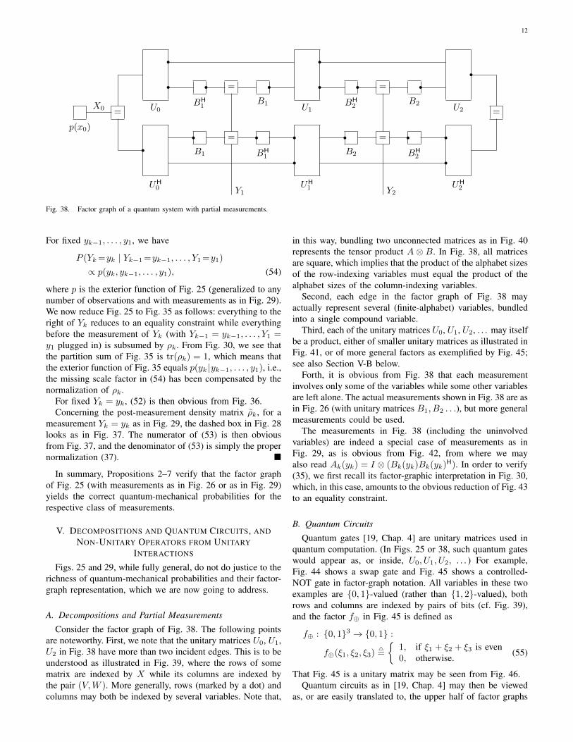
Fig. 38. Factor graph of a quantum system with partial measurements.

For fixed yk�1, . . . , y1, we have

P (Yk

=yk

| Yk�1=y

k�1, . . . , Y1=y1)

/ p(yk

, yk�1, . . . , y1), (54)

where p is the exterior function of Fig. 25 (generalized to anynumber of observations and with measurements as in Fig. 29).We now reduce Fig. 25 to Fig. 35 as follows: everything to theright of Y

k

reduces to an equality constraint while everythingbefore the measurement of Y

k

(with Yk�1 = y

k�1, . . . , Y1 =

y1 plugged in) is subsumed by ⇢k

. From Fig. 30, we see thatthe partition sum of Fig. 35 is tr(⇢

k

) = 1, which means thatthe exterior function of Fig. 35 equals p(y

k

|yk�1, . . . , y1), i.e.,

the missing scale factor in (54) has been compensated by thenormalization of ⇢

k

.For fixed Y

k

= yk

, (52) is then obvious from Fig. 36.Concerning the post-measurement density matrix ⇢

k

, for ameasurement Y

k

= yk

as in Fig. 29, the dashed box in Fig. 28looks as in Fig. 37. The numerator of (53) is then obviousfrom Fig. 37, and the denominator of (53) is simply the propernormalization (37). ⌅

In summary, Propositions 2–7 verify that the factor graphof Fig. 25 (with measurements as in Fig. 26 or as in Fig. 29)yields the correct quantum-mechanical probabilities for therespective class of measurements.

V. DECOMPOSITIONS AND QUANTUM CIRCUITS, ANDNON-UNITARY OPERATORS FROM UNITARY

INTERACTIONS

Figs. 25 and 29, while fully general, do not do justice to therichness of quantum-mechanical probabilities and their factor-graph representation, which we are now going to address.

A. Decompositions and Partial MeasurementsConsider the factor graph of Fig. 38. The following points

are noteworthy. First, we note that the unitary matrices U0, U1,U2 in Fig. 38 have more than two incident edges. This is to beunderstood as illustrated in Fig. 39, where the rows of somematrix are indexed by X while its columns are indexed bythe pair (V,W ). More generally, rows (marked by a dot) andcolumns may both be indexed by several variables. Note that,

in this way, bundling two unconnected matrices as in Fig. 40represents the tensor product A ⌦ B. In Fig. 38, all matricesare square, which implies that the product of the alphabet sizesof the row-indexing variables must equal the product of thealphabet sizes of the column-indexing variables.

Second, each edge in the factor graph of Fig. 38 mayactually represent several (finite-alphabet) variables, bundledinto a single compound variable.

Third, each of the unitary matrices U0, U1, U2, . . . may itselfbe a product, either of smaller unitary matrices as illustrated inFig. 41, or of more general factors as exemplified by Fig. 45;see also Section V-B below.

Forth, it is obvious from Fig. 38 that each measurementinvolves only some of the variables while some other variablesare left alone. The actual measurements shown in Fig. 38 are asin Fig. 26 (with unitary matrices B1, B2 . . .), but more generalmeasurements could be used.

The measurements in Fig. 38 (including the uninvolvedvariables) are indeed a special case of measurements as inFig. 29, as is obvious from Fig. 42, from where we mayalso read A

k

(yk

) = I ⌦ (Bk

(yk

)Bk

(yk

)

H). In order to verify

(35), we first recall its factor-graphic interpretation in Fig. 30,which, in this case, amounts to the obvious reduction of Fig. 43to an equality constraint.

B. Quantum CircuitsQuantum gates [19, Chap. 4] are unitary matrices used in

quantum computation. (In Figs. 25 or 38, such quantum gateswould appear as, or inside, U0, U1, U2, . . . ) For example,Fig. 44 shows a swap gate and Fig. 45 shows a controlled-NOT gate in factor-graph notation. All variables in these twoexamples are {0, 1}-valued (rather than {1, 2}-valued), bothrows and columns are indexed by pairs of bits (cf. Fig. 39),and the factor f� in Fig. 45 is defined as

f� : {0, 1}3 ! {0, 1} :

f�(⇠1, ⇠2, ⇠3)4=

⇢1, if ⇠1 + ⇠2 + ⇠3 is even0, otherwise. (55)

That Fig. 45 is a unitary matrix may be seen from Fig. 46.Quantum circuits as in [19, Chap. 4] may then be viewed

as, or are easily translated to, the upper half of factor graphs

13

X r V

W

Fig. 39. Matrix with row index X and columns indexed by the pair (V,W ).(E.g., X takes values in {0, 1, 2, 3} while V and W are both binary.)

A

r

B

r

A⌦B

Fig. 40. Tensor product of matrices A and B.

qqAAAAA q�

����

qFig. 41. Decomposition of a unitary matrix into smaller unitary matrices.Line switching as in the inner dashed box is itself a unitary matrix, cf. Fig. 44.

BHk r

=

Bk r

Ak

=

Yk

Bk

r=

BHk

rAH

k

Fig. 42. Measurements in Fig. 38 as a special case of Fig. 29.

Xk,1

Xk,2

BHk r

=

Bk r

=

Yk

= =

Bk

r=

BHk

rX 0k,2

X 0k,1

f=

Fig. 43. The exterior function of the dashed box isf=

�(xk,1, xk,2), (x0

k,1, x0k,2)

�= f=(xk,1, x0

k,1)f=(xk,2, x0k,2).

r@@@r �

��

Fig. 44. Swap gate.

r=

r �

Fig. 45. Controlled-NOT gate.

r= =

r � �=

r=

r=

Fig. 46. Proof that Fig. 45 is unitary: the exterior functions left and rightare equal.

14

as in Fig. 38. (However, this upper half cannot, by itself,properly represent the joint probability distribution of severalmeasurements.)

C. Non-unitary Operators from Unitary InteractionsUp to now, we have considered systems composed from

only two elements: unitary evolution and measurement. (Therole and meaning of the latter continues to be debated, see alsoSection VI.) However, a natural additional element is shownin Fig. 47, where a primary quantum system interacts oncewith a secondary quantum system.

(The secondary quantum system might be a stray particlethat arrives from “somewhere”, interacts with the primarysystem, and travels off to somewhere else. Or, with exchangedroles, the secondary system might be a measurement apparatusthat interacts once with a particle of interest.)

Closing the dashed box in Fig. 47 does not, in general,result in a unitary operator. Clearly, the exterior function ofthe dashed box in Fig. 47 can be represented as in Fig. 48,which may be viewed as a measurement as in Fig. 29 withunknown result Y . Conversely, it is a well-known result thatany operation as in Fig. 48, subject only to the condition

X

y

E(y)HE(y) = I (56)

(corresponding to (35) and Fig. 30), can be represented asa marginalized unitary interaction as in Fig. 47, cf. [19,Box 8.1]).

It seems natural to conjecture that classicality emerges outof such marginalized unitary interactions, as has been proposedby Zurek [33], [34] and others.

Finally, we mention some standard terminology associatedwith Fig. 48. For fixed Y = y, E(y) is a matrix, and thesematrices in Fig. 48 are called Kraus operators (cf. the operator-sum representation in [19, Sec. 8.2.3]). The exterior functionof the dashed box in Fig. 48, when viewed as a matrix withrows indexed by (

˜X, ˜X 0) and columns indexed by (X,X 0

), iscalled Liouville superoperator; when viewed as a matrix withrows indexed by (X, ˜X) and columns indexed by (X 0, ˜X 0

), itis called Choi matrix (see, e.g., [18]).

VI. MEASUREMENTS RECONSIDERED

Our tour through quantum-mechanical concepts followedthe traditional route where “measurement” is an unexplainedprimitive. However, based on the mentioned correspondencebetween Fig. 48 and Fig. 47, progress has been made inunderstanding measurement as interaction [35], [36].

There thus emerges a view of quantum mechanics funda-mentally involving only unitary transforms and marginaliza-tion. This view is still imperfectly developed (cf. [36]), butthe basic idea can be explained quite easily.

A. Projection MeasurementsThe realization of a projection measurement by a unitary

interaction is exemplified in Fig. 49. As will be detailed below,Fig. 49 (left) is a unitary interaction as in Fig. 47 while Fig. 49

X

r˜Xr

r rp(⇠)

⇠=

r rX 0 r

r˜X 0

=

Fig. 47. Two quantum systems interact unitarily. (All unlabeled boxes areunitary matrices.) The resulting exterior function of the dashed box can berepresented as in Fig. 48.

XE r ˜X

Y

X 0

EH

r ˜X 0

Fig. 48. Factor graph of a general quantum operation using Kraus operators.Such an operation may be viewed as a measurement (as in Fig. 29) withunknown result Y .

(right) is a projection measurement (with unknown result ⇣).We will see that the exterior functions of Fig. 49 (left) andFig. 49 (right) are equal.

All variables in Fig. 49 (left) take values in the set{0, . . . ,M�1} (rather than in {1, . . . ,M}) and the box la-beled “�” generalizes (55) to

f� : {0, . . . ,M�1}3 ! {0, 1} :

f�(⇠1, ⇠2, ⇠3)4=

⇢1, if (⇠1 + ⇠2 + ⇠3) mod M = 0

0, otherwise. (57)

We first note that the two inner dashed boxes in Fig. 49(left) are unitary matrices, as is easily verified from Fig. 46.Therefore, Fig. 49 (left) is indeed a special case of Fig. 47.

The key step in the reduction of Fig. 49 (left) to Fig. 49(right) is shown in Fig. 50, which in turn can be verified asfollows: the product of the two factors in the box in Fig. 50(left) is zero unless both

⇠ + ⇣ + ˜⇠ = 0 mod M (58)

and⇠ + ⇣ 0 + ˜⇠ = 0 mod M, (59)

which is equivalent to ⇣ = ⇣ 0 and (58). For fixed ⇠ and ⇣,(58) allows only one value for ˜⇠, which proves the reductionin Fig. 50.

15

X

BH

r=

B

r ˜X

p(⇠)

⇠=

�

�

=

X 0 Br=

BHr ˜X 0

rr

rr

=

X

BH

r=

B

r ˜X

⇣

=

⇣ 0

X 0 Br=

BHr ˜X 0

Fig. 49. Projection measurement (with unitary matrix B) as marginalized unitary interaction. Left: unitary interaction as in Fig. 47; the inner dashed boxesare unitary (cf. Fig. 45). Right: resulting projection measurement (with unknown result ⇣). The exterior functions left and right are equal.

�

⇣

⇠ ˜⇠�

⇣ 0

=

⇣

=

⇣ 0

Fig. 50. Proof of the reduction in Fig. 49.

X

BH

r=

B

r ˜X

=

⇣

p(y|⇣)

Y

X 0 Br=

BHr ˜X 0

Fig. 51. Observing the post-measurement variable ⇣ in Fig. 49 (right) via a(classical) “channel” p(y|⇣).

The generalization from fixed ⇠ to arbitrary p(⇠) is straight-forward.

We have thus established that the (marginalized) unitary in-teraction in Fig. 49 (left) acts like the projection measurementin Fig. 49 (right) and thereby creates the random variable ⇣.

Moreover, projection measurements are repeatable, i.e., re-peating the same measurement (immediately after the first

measurement) leaves the measured quantum system un-changed. (In fact, this property characterizes projection mea-surements.) Therefore, the random variable ⇣ is an objec-tive property of the quantum system after the measure-ment/interaction; it can be cloned, and it can, in principle,be observed, either directly or via some “channel” p(y|⇣),as illustrated in Fig. 51. The conditional-probability factorp(y|⇣) allows, in particular, that ⇣ is not fully observable,i.e., different values of ⇣ may lead to the same observationY = y.

B. General Measurements

A very general form of (indirect) measurement is shown inFig. 52, which is identical to Fig. 47 except for the observablevariable Y . The figure is meant to be interpreted as follows.Some primary quantum system (with variables X,X 0, ˜X, ˜X 0)interacts once with a secondary quantum system, which inturn is measured by a projection measurement as in Fig. 51.It is not difficult to verify (e.g., by adapting the procedure in[19, Box 8.1]) that an interaction as in Fig. 52 can realize anymeasurement as in Fig. 29.

VII. RANDOM VARIABLES RECONSIDERED

Up to Section V-B, all random variables were either part ofthe initial conditions (such as X0 in Fig. 38) or else created bymeasurements (such as Y1 and Y2 in Fig. 38). In Section VI,we have outlined an emerging view of quantum mechanicswhere measurements are no longer undefined primitives, butexplained as unitary interactions.

We now re-examine the creation of random variables in thissetting. We find that, fundamentally, random variables are notcreated by interaction, but by the end of it. The mechanismis illustrated in Fig. 53: a quantum system with potentiallyentangled variables (X,X 0

) and (⇠, ⇠0) splits such that (X,X 0)

and (⇠, ⇠0) do not interact in the future. In this case, (⇠, ⇠0) canbe marginalized away by closing the dashed box in Fig. 53,which amounts to forming the density matrix ⇢(x, x0

) as a

16

X

r˜Xr

p(⇠)

⇠=

r rX 0 r ˜X 0

rBH

r=

Br=

B

r=

BHr⇣

p(y|⇣)

Y

Fig. 52. General measurement as unitary interaction and marginalization. The matrix B and the unlabeled solid boxes are unitary matrices. The part withthe dashed edges is redundant.

p(x0)

X0=

r X

r

rX 0

⇠

=

⇠0

⇢(x, x0)

r=

r

Fig. 53. Marginalization over ⇠ turns ⇠ into a random variable. (The unlabeled boxes are unitary matrices.)

p(x0)

X0=

...rr

r...

r⇠1

=

...

@@@@

��

��

...

⇠2

=

......

@@@@

��

��

......

⇠3

=

...

...

. . .

Fig. 54. Stochastic process without measurement. The rectangular boxes are unitary operators.

17

⇢codeX1

X 01

�

...

Xn

X 0n

�

˜X1

˜X 01

...

˜Xn

˜X 0n

Y1 · · · Ym

=

=

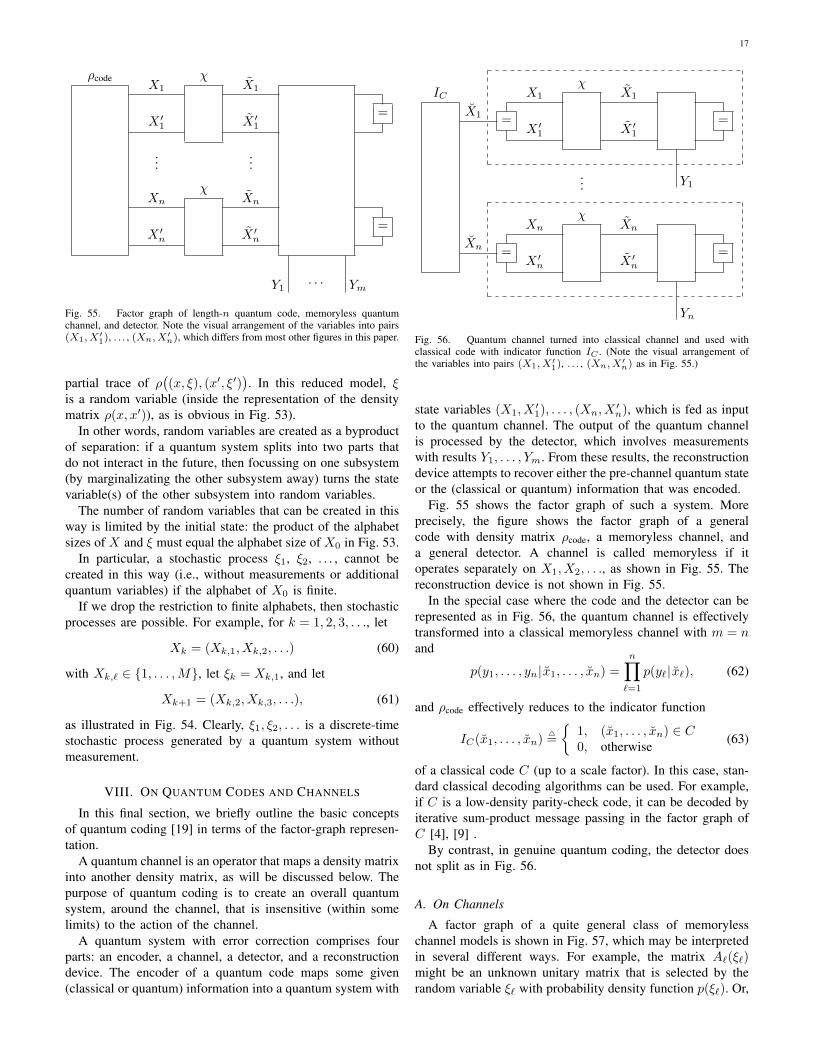
Fig. 55. Factor graph of length-n quantum code, memoryless quantumchannel, and detector. Note the visual arrangement of the variables into pairs(X1, X0

1), . . . , (Xn, X0n), which differs from most other figures in this paper.

partial trace of ⇢�(x, ⇠), (x0, ⇠0)

�. In this reduced model, ⇠

is a random variable (inside the representation of the densitymatrix ⇢(x, x0

)), as is obvious in Fig. 53).In other words, random variables are created as a byproduct

of separation: if a quantum system splits into two parts thatdo not interact in the future, then focussing on one subsystem(by marginalizating the other subsystem away) turns the statevariable(s) of the other subsystem into random variables.

The number of random variables that can be created in thisway is limited by the initial state: the product of the alphabetsizes of X and ⇠ must equal the alphabet size of X0 in Fig. 53.

In particular, a stochastic process ⇠1, ⇠2, . . . , cannot becreated in this way (i.e., without measurements or additionalquantum variables) if the alphabet of X0 is finite.

If we drop the restriction to finite alphabets, then stochasticprocesses are possible. For example, for k = 1, 2, 3, . . ., let

Xk

= (Xk,1, Xk,2, . . .) (60)

with Xk,`

2 {1, . . . ,M}, let ⇠k

= Xk,1, and let

Xk+1 = (X

k,2, Xk,3, . . .), (61)

as illustrated in Fig. 54. Clearly, ⇠1, ⇠2, . . . is a discrete-timestochastic process generated by a quantum system withoutmeasurement.

VIII. ON QUANTUM CODES AND CHANNELS

In this final section, we briefly outline the basic conceptsof quantum coding [19] in terms of the factor-graph represen-tation.

A quantum channel is an operator that maps a density matrixinto another density matrix, as will be discussed below. Thepurpose of quantum coding is to create an overall quantumsystem, around the channel, that is insensitive (within somelimits) to the action of the channel.

A quantum system with error correction comprises fourparts: an encoder, a channel, a detector, and a reconstructiondevice. The encoder of a quantum code maps some given(classical or quantum) information into a quantum system with

IC

˘X1

˘Xn

...

=

X1

X 01

�

Xn

X 0n

�

=

˜X1

˜X 01

Y1

˜Xn

˜X 0n

Yn

=

=

Fig. 56. Quantum channel turned into classical channel and used withclassical code with indicator function IC . (Note the visual arrangement ofthe variables into pairs (X1, X0

1), . . . , (Xn, X0n) as in Fig. 55.)

state variables (X1, X 01), . . . , (Xn

, X 0n

), which is fed as inputto the quantum channel. The output of the quantum channelis processed by the detector, which involves measurementswith results Y1, . . . , Ym

. From these results, the reconstructiondevice attempts to recover either the pre-channel quantum stateor the (classical or quantum) information that was encoded.

Fig. 55 shows the factor graph of such a system. Moreprecisely, the figure shows the factor graph of a generalcode with density matrix ⇢code, a memoryless channel, anda general detector. A channel is called memoryless if itoperates separately on X1, X2, . . ., as shown in Fig. 55. Thereconstruction device is not shown in Fig. 55.

In the special case where the code and the detector can berepresented as in Fig. 56, the quantum channel is effectivelytransformed into a classical memoryless channel with m = nand

p(y1, . . . , yn|x1, . . . , xn

) =

nY

`=1

p(y`

|x`

), (62)

and ⇢code effectively reduces to the indicator function

IC

(x1, . . . , xn

)

4=

⇢1, (x1, . . . , xn

) 2 C0, otherwise (63)

of a classical code C (up to a scale factor). In this case, stan-dard classical decoding algorithms can be used. For example,if C is a low-density parity-check code, it can be decoded byiterative sum-product message passing in the factor graph ofC [4], [9] .

By contrast, in genuine quantum coding, the detector doesnot split as in Fig. 56.

A. On ChannelsA factor graph of a quite general class of memoryless

channel models is shown in Fig. 57, which may be interpretedin several different ways. For example, the matrix A

`

(⇠`

)

might be an unknown unitary matrix that is selected by therandom variable ⇠

`

with probability density function p(⇠`

). Or,

18

X`

A`

(⇠`

)r ˜X`

p(⇠`

)

⇠`

=

X 0`

A`

(⇠`

)

H

r ˜X 0`

�

Fig. 57. Factor graph of a general channel model (for use in Fig. 55).The node/factor p(⇠`) may be missing.

X`

A` r ˜X

`

X 0`

AH`

r ˜X 0`

�

Fig. 58. Simplified version of Fig. 57 for fixed ⇠`.

in an other interpretation, Fig. 57 without the node/factor p(⇠`

)

is a general operation as in Fig. 48.Many quantum coding schemes distinguish only between

“no error” in position ` (i.e., A`

(⇠`

) = I) and “perhapssome error” (where A

`

(⇠`

) is arbitrary, but nonzero); no otherdistinction is made and no prior p(⇠

`

) is assumed. For theanalysis of such schemes, Fig. 57 can often be replaced bythe simpler Fig. 58. In such an analysis, it may be helpfulto express the (fixed, but unknown) matrix A

`

in Fig. 58 insome pertinent basis. For example, any matrix A 2 C2⇥2 canbe written as

A =

3X

k=0

wk

�k

(64)

with w0, . . . , w3 2 C and where �0, . . . ,�3 are the Paulimatrices

�04=

✓1 0

0 1

◆, (65)

�14=

✓0 1

1 0

◆, (66)

�24=

✓0 �ii 0

◆, (67)

and�3

4=

✓1 0

0 �1

◆. (68)

The matrices �0, . . . ,�3 are unitary and Hermitian, and theyform a basis of C2⇥2.

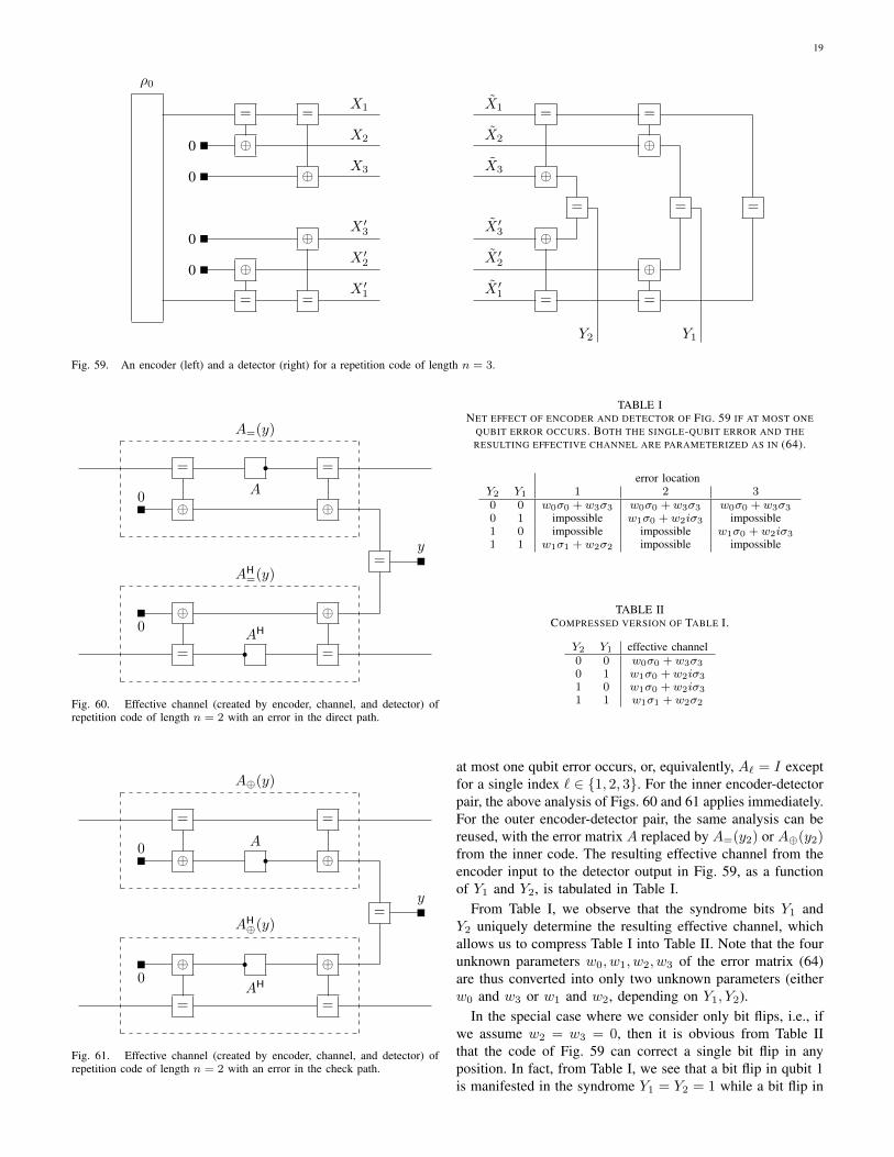
B. Repetition Codes of Length 2 and 3Fig. 59 (left) shows the factor graph of an encoder of a

simple code of length n = 3. All variables in this factor graphare binary, and the initial density matrix ⇢0 is arbitrary. Notethat this encoder can be realized with two controlled-not gates(cf. Fig. 45) and two ancillary qubits with fixed initial statezero.

A detector for this code is shown in Fig. 59 (right). Thisdetector can be realized with two controlled-not gates and twoqubit measurements. The unitary part of this detector invertsthe unitary part of the encoder, and the measured bits Y1

and Y2 (henceforth called syndrome bits) correspond to theancillary qubits in the encoder.

The code of Fig. 59 is not very useful in itself, but it sufficesto demonstrate some basic ideas of quantum coding and itfurther illustrates the use of factor graphs. Moreover, once thissimple code is understood, it is easy to proceed to the Shorcode [19], which can correct an arbitrary single-qubit error.

The encoder-detector pair of Fig. 59 may be viewed astwo nested encoder-detector pairs for a repetition code oflength n = 2: the inner encoder-detector pair produces thesyndrome bit Y2, and the outer encoder-detector pair producesthe syndrome bit Y1.

Therefore, we now consider the net effect of the encoder,the channel, and the detector of a repetition code of lengthn = 2 as shown in Figs. 60 and 61. We assume that at mostone qubit error occurs, either in the direct path (as in Fig. 60)or in the check path (as in Fig. 61). This single potential erroris a general nonzero matrix A 2 C2⇥2 (as in Fig. 58) withrow and column indices in {0, 1}.

For fixed Y = y, the net effect of the encoder, the channel,and the detector amounts to a matrix A=(y) or A�(y) corre-sponding to the dashed boxes in Figs. 60 and 61, respectively.

If A = I (i.e., if there is no error), we necessarily haveY = 0 and A=(0) = A�(0) = I . For general nonzero A,parameterized as in (64), we have

A=(0) =

✓A(0, 0) 0

0 A(1, 1)

◆(69)

= w0�0 + w3�3, (70)

i.e., the projection of A onto the space spanned by �0 and �3,and

A=(1) =

✓0 A(0, 1)

A(1, 0) 0

◆(71)

= w1�1 + w2�2, (72)

i.e., the projection of A onto the space spanned by �1 and �2.Moreover,

A�(0) = A=(0), (73)

and

A�(1) =

✓A(1, 0) 0

0 A(0, 1)

◆(74)

= �1A=(1) (75)= w1�0 + w2i�3. (76)

We now return to Fig. 59, which we consider as two nestedencoder-detector pairs as in Figs. 60 and 61. We assume that

19

⇢0

= =

X1

0 � X2

0 � X3

0 �X 0

3

0 �X 0

2

= =

X 01

˜X1= =

˜X2 �˜X3 �

=

Y2

=

Y1

=

˜X 03 �

˜X 02 �

˜X 01

= =

Fig. 59. An encoder (left) and a detector (right) for a repetition code of length n = 3.

=

A

r=

0

� �

A=(y)

=

y

0

� �

=

AHr=

AH=(y)

Fig. 60. Effective channel (created by encoder, channel, and detector) ofrepetition code of length n = 2 with an error in the direct path.

= =

0

�A r �

A�(y)

=

y

0

�AH

r �

= =

AH�(y)

Fig. 61. Effective channel (created by encoder, channel, and detector) ofrepetition code of length n = 2 with an error in the check path.

TABLE INET EFFECT OF ENCODER AND DETECTOR OF FIG. 59 IF AT MOST ONE

QUBIT ERROR OCCURS. BOTH THE SINGLE-QUBIT ERROR AND THERESULTING EFFECTIVE CHANNEL ARE PARAMETERIZED AS IN (64).

error locationY2 Y1 1 2 30 0 w0�0 + w3�3 w0�0 + w3�3 w0�0 + w3�30 1 impossible w1�0 + w2i�3 impossible1 0 impossible impossible w1�0 + w2i�31 1 w1�1 + w2�2 impossible impossible

TABLE IICOMPRESSED VERSION OF TABLE I.

Y2 Y1 effective channel0 0 w0�0 + w3�30 1 w1�0 + w2i�31 0 w1�0 + w2i�31 1 w1�1 + w2�2

at most one qubit error occurs, or, equivalently, A`

= I exceptfor a single index ` 2 {1, 2, 3}. For the inner encoder-detectorpair, the above analysis of Figs. 60 and 61 applies immediately.For the outer encoder-detector pair, the same analysis can bereused, with the error matrix A replaced by A=(y2) or A�(y2)from the inner code. The resulting effective channel from theencoder input to the detector output in Fig. 59, as a functionof Y1 and Y2, is tabulated in Table I.

From Table I, we observe that the syndrome bits Y1 andY2 uniquely determine the resulting effective channel, whichallows us to compress Table I into Table II. Note that the fourunknown parameters w0, w1, w2, w3 of the error matrix (64)are thus converted into only two unknown parameters (eitherw0 and w3 or w1 and w2, depending on Y1, Y2).

In the special case where we consider only bit flips, i.e., ifwe assume w2 = w3 = 0, then it is obvious from Table IIthat the code of Fig. 59 can correct a single bit flip in anyposition. In fact, from Table I, we see that a bit flip in qubit 1is manifested in the syndrome Y1 = Y2 = 1 while a bit flip in

20

= = H = =

X1

�0

X2

�0

X3

0

� H = =

X4

�0

X5

�0

X6

� H = =

X7

�0

X8

�0

X9

Fig. 62. Encoder of the Shor code. The figure shows only the upper half ofthe factor graph.

qubit 2 or in qubit 3 has no effect on the resulting effectivechannel, except for an irrelevant scale factor. However, wewish to be able to deal with more general errors.

C. Correcting a Single Error: The Shor CodeFig. 62 shows an encoder of the Shor code [19]. The

figure shows only the upper half of the factor graph (i.e.,the quantum circuit). The nodes labeled “H” represent thenormalized Hadamard matrix

H4=

1p2

✓1 1

1 �1

◆, (77)

which is symmetric and unitary and satisfies H�1 = �3H ,and H�2 = ��2H . Note that this encoder uses four copies ofthe encoder in Fig. 59: three independent inner encoders areglued together with an outer encoder.

As a detector, we use the obvious generalization of Fig. 59(right), i.e., the mirror image of the encoder.

This encoder-detector pair is easily analyzed using theresults of Section VIII-B. For this analysis, we assume that atmost a single qubit error occurs (i.e., A

`

6= I for at most oneindex ` 2 {1, . . . , 9}). In consequence, two of the three innerencoder-detector pairs are error-free and reduce to an identitymatrix. The remaining inner encoder-detector pair is describedby Table II. The multiplication by H both in the encoder andin the detector changes Table II to Table III. Note that theresulting effective channel is either of the form a�0 + b�1 orc�2 + d�3, and the detector knows which case applies.

The outer encoder-detector pair thus sees an error in atmost one position, and the potential error is described byTable II, except that the underlying channel is not (64), but asin Table III. Revisiting Table II accordingly yields Table IV,which describes the net effect of the outer encoder-detectorpair. In any case, the resulting effective channel is of theform ↵�

k

for some nonzero ↵ 2 C and some (known)k 2 {0, 1, 2, 3}. In other words, the effective channel (from

TABLE IIIEFFECTIVE CHANNEL OF TABLE II

WITH PRE- AND POST-MULTIPLICATION BY H .

Y2 Y1 effective channel0 0 w0�0 + w3�10 1 w1�0 + w2i�11 0 w1�0 + w2i�11 1 w1�3 � w2�2

TABLE IVNET EFFECT OF ENCODER (AS IN FIG. 62) AND MIRROR-IMAGE DETECTOR

OF SHOR CODE, ASSUMING THAT AT MOST ONE QUBIT ERROR OCCURS.“INNER CODE” REFERS TO THE INNER ENCODER-DETECTOR PAIR WITH

THE POTENTIAL ERROR.

outer detector effect of inner codeY2 Y1 a�0 + b�1 c�2 + d�30 0 a�0 d�30 1 b�0 ci�31 0 b�0 ci�31 1 b�1 c�2

encoder input to detector output) is fully determined by the 8syndrome bits, up to an irrelevant scale factor. In consequence,the (arbitrary) original quantum state can exactly be restored.

IX. CONCLUSION

We have proposed factor graphs for quantum-mechanicalprobabilities involving any number of measurements, both forbasic projection measurements and for general measurements.Our factor graphs represent factorizations of complex-valuedfunctions q as in (3) such that the joint probability distributionof all random variables (in a given quantum system) is amarginal of q. Therefore (and in contrast to other graphicalrepresentations of quantum mechanics), our factor graphs arefully compatible with standard statistical models. We have alsointerpreted a variety of concepts and quantities of quantummechanics in terms of factorizations and marginals of suchfunctions q. We have further illustrated the use of factor graphsby an elementary introduction to quantum coding.

In Appendix A, we offer some additional remarks on theprior literature. In Appendix B, we derive factor graphs forthe Wigner–Weyl representation. In Appendix C, we point outthat the factor graphs of this paper are amenable (at least inprinciple) to Monte Carlo algorithms.

We hope that our approach makes quantum-mechanicalprobabilities more accessible to non-physicists and furtherpromotes the exchange of concepts and algorithms betweenphysics, statistical inference, and error correcting codes in thespirit of [5], [26], [37].

Finally, we mention that the factor graphs of this paper havebeen used in [24] for estimating the information rate of certainquantum channels, and iterative sum-product message passingin such factor graphs is considered in [25].

21

���HHH

v w���HHH

Fig. 63. Tensor network notation. Left: bra (row vector); right: ket (columnvector). Note that the meaning of the symbol depends on its orientation onthe page.

APPENDIX AADDITIONAL REMARKS ABOUT RELATED WORK

A. Tensor NetworksWith hindsight, the factor graphs of this paper are quite

similar to tensor networks [16]–[18], [20], which have recentlymoved into the heart of theoretical physics [37].

Tensor networks (and related graphical notation) have beenused to represent the wave function | i of several entangledspins at a given time. In general, the resulting states are calledtensor network states (TNS), but depending on the structureof the tensor network, more specialized names like matrixproduct states (MPS), tree tensor states (TTS), etc., are used.A very nice overview of this line of work is given in thesurvey paper by Cirac and Verstraete [16], which also explainsthe connection of TNS to techniques like the density matrixrenormalization group (DMRG), the multiscale entanglementrenormalization ansatz (MERA), and projected entangled pairstates (PEPS).

If such tensor diagrams are used to represent quantities likeh | i or h |�2�4| i (see, e.g., Fig. 2 in [16]), they havetwo conjugate parts, like the factor graphs in the present paper(Fig. 13, etc.).

It should be noted, however, that the graphical conventionsof tensor networks differ from factor graphs in this point: themeaning of a tensor network diagram frequently depends onits orientation on the page (see, e.g., [18]), and exchanging leftand right amounts to a Hermitian transposition, as illustratedin Fig. 63.

B. Quantum Bayesian Networks and Quantum Belief Propa-gation

Whereas the present paper uses conventional Forney fac-tor graphs (with standard semantics and algorithms), variousauthors have proposed modified graphical models or specific“quantum algorithms” for quantum mechanical quantities [22],[38], [39]. Such graphical models (or algorithms) are notcompatible with standard statistical models; they are not basedon (3) and they lack Proposition 1.

C. Keldysh FormalismThere are some high-level similarities between the graphical

models in the present paper and some diagrams that appearin the context of the Keldysh formalism (see, e.g., [40]); inparticular, both have “two branches along the time axis.”

However, there are also substantial dissimilarities: first,the diagrams in the Keldysh formalism also have a thirdbranch along the imaginary axis; second, our factor graphsare arguably more explicit than the diagrams in the Keldyshformalism.

D. Normal Factor Graphs, Classical Analytical Mechanics,and Feynman Path Integrals

In [41], it is shown how Forney factor graphs (= normal fac-tor graphs) can be used for computations in classical analyticalmechanics. In particular, it is shown how to represent theaction S(x) of a trajectory x and how to use the stationary-sumalgorithm for finding the path where the action is stationary.

It is straightforward to modify the factor graphs in [41] inorder to compute, at least in principle, Feynman path integrals,where exp

�i

~S(x)�

is integrated over a suitable domain ofpaths x: essentially by replacing the function nodes f( · )in [41] by exp

�i

~f( · )�, and by replacing the stationary-sum

algorithm by standard sum-product message passing [4].

APPENDIX BWIGNER–WEYL REPRESENTATION

The Wigner–Weyl representation of quantum mechanicsexpresses the latter in terms of the “phase-space” coordinatesq and p (corresponding to the position and the momentum,respectively, of classical mechanics). When transformed intothis representation, the density matrix turns into a real-valuedfunction.

So far in this paper, all variables were assumed to takevalues in some finite set without any structure. However, theWigner–Weyl representation requires that both the originalcoordinates X and X 0 and the new coordinates p and qcan be added and subtracted and admit a Fourier transformas in (81) and (85) below. In the following, we assumeX

k

, X 0k

,pk

,qk

2 RN for all k.In a factor graph with continuous variables, the exterior

function of a box is defined by integrating over the internalvariables, i.e., the sum in (5) and (6) is replaced by an integral.Moreover, the equality constraint function (9) becomes

f=(x1, . . . , xn

) = �(x1 � x2) · · · �(xn�1 � xn

), (78)

where � is the Dirac delta. Finally, matrices (cf. Section II-B)are generalized to operators, i.e., the sums in (11) and (12)are replaced by integrals.

The transformation to the Wigner–Weyl representation usesan operator W that will be described below. Factor graphs forthe Wigner–Weyl representation may then be obtained fromthe factor graphs in Sections III–V by a transformation as inFig. 64. The example in this figure is a factor graph as inFig. 25 with a single measurement, but the generalization toany number of measurements is obvious. Starting from theoriginal factor graph (top in Fig. 64), we first insert neutralfactors (identity operators) factored as I = WW�1 as shownin Fig. 64 (middle); clearly, this manipulation does not changep(y). We then regroup the factors as in Fig. 64 (bottom), whichagain leaves p(y) unchanged. The Wigner–Weyl factor graph isthen obtained by closing the dashed boxes in Fig. 64 (bottom).(The Wigner–Weyl representation has thus been obtained as a“holographic” factor graph transform as in [29], [30].)

The operator W encodes the relations

X = q� s (79)X 0

= q+ s (80)

22

⇢

r X0

X 00

U r

UH

rX1

X 01

Y

X2

X 02

=

⇢

r X0

X 00

W W�1

I

U r

UH

r W W�1

I

X1

X 01

Y

X2

X 02

W W�1

I

=

⇢

rW

initial state µW

q0

p0W�1

U r

UH

r W

evolution

q1

p1W�1

Y

W

measurement

q2

p2W�1

=

termination

Fig. 64. Wigner–Weyl transform of a quantum factor graph with W as defined in Fig. 65. Top: quantum system with a single measurement yielding Y .Middle: inserting neutral factors (identity operators) I = WW�1 does not change the exterior function p(y). Bottom: closing the dashed boxes yields thefactor graph of the Wigner–Weyl representation. The termination box reduces to an empty box.

X

X 0

q

sFr p

W

q

pF�1r s

X

X 0

W�1

Fig. 65. Factor graphs of Wigner–Weyl transformation operator W (left) and its inverse (right). The unlabeled box inside W represents the factor (82); theunlabeled box inside W�1 represents the factor (84).

23

and the Fourier transform with kernel

F(s,p) =

✓1

⇡~

◆N

e(i/~)2pTs. (81)

For the purpose of this paper, ~ (the reduced Planck constant)is an arbitrary positive scale factor.

The factor-graph representation of the operator W (shownleft in Fig. 65) consists of two factors: the first factor is

��x� (q� s)

���x0 � (q+ s)

�, (82)

which encodes the contraints (79) and (80); the second factoris the Fourier kernel (81).

The factor-graph representation of W�1 (right in Fig. 65)consists of the inverse Fourier transform kernel

F�1(s,p) = e(�i/~)2pTs (83)

and the factor

��q� 1

2

(x+ x0)

���s� 1

2

(�x+ x0)

�. (84)

Closing the “initial state” box in Fig. 64 yields the function

µW

(q,p) =

Z 1

�1

✓1

⇡~

◆N

e(i/~)2pTs⇢(q� s,q+ s) ds (85)

for q = q0 and p = p0, which is easily seen to be real (since⇢(x, x0

) = ⇢(x0, x)).Closing the “termination” box in Fig. 64 yields the function

Z 1

�1

Z 1

�1

Z 1

�1e(�i/~)2pTs �

�q� 1

2

(x+ x0)

�

��s� 1

2

(�x+ x0)

��(x� x0

) dx0 dx ds

=

Z 1

�1e(�i/~)2pTs�(s) ds (86)

= 1. (87)

The termination box thus reduces to an empty box and can beomitted.

APPENDIX CMONTE CARLO METHODS

Let f(x1, . . . , xn

) be a nonnegative real function of finite-alphabet variables x1, . . . , xn

. Many quantities of interest instatistical physics, information theory, and machine learningcan be expressed as a partition sum

Zf

4=

X

x1,...,xn

f(x1, . . . , xn

) (88)

of such a function f . The numerical computation of suchquantities is often hard. When other methods fail, good resultscan sometimes be obtained by Monte Carlo methods [43]–[45].A key quantity in such Monte Carlo methods is the probabilitymass function

pf

(x1, . . . , xn

)

4= f(x1, . . . , xn

)/Zf

. (89)

An extension of such Monte Carlo methods to functions fthat can be negative or complex was outlined in [46]. However,only the real case (where f can be negative) was addressed insome detail in [46]. We now substantiate the claim from [46]

that complex functions q as represented by the factor graphsof this paper can be handled as in the real case.

We will use the abbreviation x4= (x1, . . . , xn

), and,following [46], we define

Z|f |4=

X

x

|f(x)| (90)

and the probability mass function

p|f |(x)4=

|f(x)|Z|f |

(91)

Note that p|f | inherits factorizations (and thus factor graphs)from f . This also applies to more general distributions of theform

p(x; ⇢) / |f(x)|⇢ (92)

for 0 < ⇢ < 1.For the real case, the gist of the Monte Carlo methods of

[46] is as follows:1) Generate a list of samples x(1), . . . , x(K) either from

p|f |(x), or from a uniform distribution over x, or froman auxiliary distribution p(x; ⇢) as in (92).

2) Estimate Z (and various related quantities) from sumssuch as X

k:f(x(k))>0

f(x(k)) (93)

and X

k:f(x(k))<0

f(x(k)), (94)

or X

k:f(x(k))>0

1

f(x(k))

(95)

and X

k:f(x(k))<0

1

f(x(k))

, (96)

or, more generally,X

k:f(x(k))>0

f(x(k))

⇢1

f(x(k))

⇢2(97)

and X

k:f(x(k))<0

f(x(k))

⇢1

f(x(k))

⇢2(98)

The idea is always that the sampling probability equals thedenominator (up to a scale factor), which results in simpleexpectations for these sums. (The quantities (97) and (98) arenot actually mentioned in [46], but they arise from translatingmulti-temperature Monte Carlo methods (cf. [44], [45]) to thesetting of [46].)

Note that Step 1 above (the generation of samples) general-izes immediately to the complex case; our issue here is Step 2,where the generalization is less obvious.

Recall now that all factor graphs in Sections III–V representfunctions with the structure

q(x, x0, y) = g(x, y)g(x0, y) (99)

24

as in Fig. 13. But any such function satisfies

q(x, x0, y) = q(x0, x, y). (100)

Under any of the probability distributions in Step 1 above, aconfiguration (x, x0, y) then has the same probability as theconjugate configuration (x0, x, y) (i.e., (x, x0, y) and (x0, x, y)are so-called antithetic variates). We can thus double the list ofsamples in Step 1 by adding all the conjugate configurations.For the augmented list of samples, the sum (93) becomes

X

k:f(x(k))+f(x(k))>0

f(x(k)) + f(x(k)

), (101)

and the sums (94)–(98) can be handled analogously.

ACKNOWLEDGMENT

The material of this paper has been developing over along time. Its beginnings have benefitted from discussions,mostly long ago, with Niclas Wiberg, Justin Dauwels, FrankKschischang, and Nikolai Nefedov. More recently, we haveprofited from discussions with Ali Al-Bashabsheh, G. DavidForney, Jr., and Yongyi Mao. We also thank the reviewers of[1] and Alexey Kovalev for pointing out pertinent work in thephysics literature.

REFERENCES

[1] H.-A. Loeliger and P. O. Vontobel, “A factor-graph representation ofprobabilities in quantum mechanics,” Proc. 2012 IEEE Int. Symp. onInformation Theory, Cambridge, MA, USA, July 1–6, 2012, pp. 656–660.

[2] F. R. Kschischang, B. J. Frey, and H.-A. Loeliger, “Factor graphs and thesum-product algorithm,” IEEE Trans. Inf. Theory, vol. 47, pp. 498–519,Feb. 2001.

[3] G. D. Forney, Jr., “Codes on graphs: normal realizations,” IEEE Trans.Inf. Theory, vol. 47, no. 2, pp. 520–548, 2001.

[4] H.-A. Loeliger, “An introduction to factor graphs,” IEEE Sig. Proc. Mag.,Jan. 2004, pp. 28–41.

[5] M. Mezard and A. Montanari, Information, Physics, and Computation.Oxford University Press, 2009.

[6] M. I. Jordan, “Graphical models,” Statistical Science, vol. 19, no. 1,pp. 140–155, 2004.

[7] Ch. M. Bishop, Pattern Recognition and Machine Learning. New York:Springer Science+Business Media, 2006.

[8] D. Koller and N. Friedman, Probabilistic Graphical Models. Cambridge,MA, MIT Press, 2009.

[9] T. Richardson and R. Urbanke, Modern Coding Theory. CambrideUniversity Press, 2008.

[10] H. Wymeersch, Iterative Receiver Design. Cambridge University Press,2007.

[11] H.-A. Loeliger, J. Dauwels, Junli Hu, S. Korl, Li Ping, and F. R. Kschi-schang, “The factor graph approach to model-based signal processing,”Proceedings of the IEEE, vol. 95, no. 6, pp. 1295–1322, June 2007.

[12] H.-A. Loeliger, L. Bruderer, H. Malmberg, F. Wadehn, and N. Zalmai,“On sparsity by NUV-EM, Gaussian message passing, and Kalmansmoothing,” Information Theory & Applications Workshop, La Jolla, CA,Jan. 31 – Feb. 5, 2016.

[13] P. O. Vontobel, “The Bethe permanent of a non-negative matrix,” IEEETrans. Inf. Theory, vol. 59, pp. 1866–1901, Mar. 2013.

[14] M. Veltman, Diagrammatica: The Path to Feynman Diagrams. Cam-bridge Lecture Notes in Physics, 1994.

[15] Z.-C. Gu, M. Levin, and X.-G. Wen, “Tensor-entanglement renormal-ization group approach as a unified method for symmetry breaking andtopological phase transitions,” Phys. Rev. B, vol. 78, p. 205116, Nov.2008.

[16] J. I. Cirac and F. Verstraete, “Renormalization and tensor product statesin spin chains and lattices,” J. Phys. A: Math. and Theor., vol. 42,no. 504004, pp. 1–34, 2009.

[17] B. Coecke, “Quantum picturalism,” Contemporary Phys., vol. 51, no. 1,pp. 59–83, 2010.

[18] C. J. Wood, J. D. Biamonte, and D. J. Cory, “Tensor networks andgraphical calculus for open quantum systems,” Quantum Informationand Computation, vol. 15, pp. 759-811, 2015.

[19] M. A. Nielsen and I. L. Chuang, Quantum Computation and QuantumInformation. Cambridge University Press, 2000.

[20] G. Chiribella, G. M. D’Ariano, and P. Perinotti, “Probabilistic theorieswith purification,” Phys. Review A, vol. 81, 2010, pp. 062348-1–062348-40.

[21] R. Mori, “Holographic transformation, belief propagation and loopcalculus for generalized probabilistic theories,” Proc. 2015 IEEE Int.Symp. on Information Theory, Hong Kong, China, June 14–19, 2015.

[22] R. R. Tucci, “Quantum information theory – a quantum Bayesian netperspective,” arXiv:quant-ph/9909039v1, 1999.

[23] M. S. Leifer and D. Poulin, “Quantum graphical models and beliefpropagation,” Annals of Physics, vol. 323, no. 8, pp. 1899–1946, Aug.2008.

[24] M. X. Cao and P. O. Vontobel, “Estimating the information rate of achannel with classical input and output and a quantum state,” Proc. IEEEInt. Symp. Inf. Theory, Aachen, Germany, June 25–30, 2017. Extendedversion available from https://arxiv.org/abs/1705.01041.

[25] M. X. Cao and P. O. Vontobel, “Double-edge factor graphs: definition,properties, and examples,” submitted to 2017 IEEE Information TheoryWorkshop, May 2017. Available from https://arxiv.org/abs/1706.00752.

[26] P. O. Vontobel and H.-A. Loeliger, “On factor graphs and electricalnetworks,” in Mathematical Systems Theory in Biology, Communication,Computation, and Finance, J. Rosenthal and D. S. Gilliam, eds., IMAVolumes in Math. & Appl., Springer Verlag, 2003, pp. 469–492.

[27] P. Cvitanovic, Group Theory: Birdtracks, Lie’s, and Exceptional Groups.Princeton Univ. Press, 2008.

[28] E. Peterson, “Unshackling linear algebra from linear notation,”arXiv:0910.1362, 2009.

[29] G. D. Forney, Jr., and P. O. Vontobel, “Partition functions of normalfactor graphs,” Information Theory & Applications Workshop, La Jolla,CA, USA, Feb. 6–11, 2011.

[30] A. Al-Bashabsheh and Y. Mao, “Normal factor graphs and holographictransformations,” IEEE Trans. Inf. Theory, vol. 57, no. 2, pp. 752–763,Feb. 2011.

[31] A. Al-Bashabsheh, Y. Mao, and P. O. Vontobel, “Normal factor graphs:a diagrammatic approach to linear algebra,” Proc. IEEE Int. Symp. Inf.Theory, St. Petersburg, Russia, Jul. 31–Aug. 5, 2011, pp. 2178–2182.

[32] K. Kraus, States, Effects and Operations. Lecture Notes in Physics.Berlin: Springer-Verlag, 1983.

[33] W. H. Zurek, “Decoherence, einselection, and the quantum origins ofthe classical,” Rev. Mod. Phys., vol. 75, no. 3, pp. 715–775, July 2003.

[34] W. H. Zurek, “Quantum Darwinism,” Nature Physics, vol. 5, pp. 181–188, March 2009.

[35] H.-P. Breuer and F. Petruccione, Open Quantum Systems. Oxford Uni-versity Press, New York, NY, 2002.

[36] M. Schlosshauer, “Decoherence, the measurement problem, and interpre-tations of quantum mechanics,” Rev. Mod. Phys., vol. 76, pp. 1267–1305,Oct. 2004.

[37] R. Cowen, “Space, time, entanglement,” Nature, vol. 527, pp. 290–293,Nov. 2015.

[38] M. G. Parker, “Quantum factor graphs,’ Ann. Telecomm. vol. 56, no. 7–8, pp. 472–483, 2001.

[39] M. S. Leifer, D. Poulin, “Quantum graphical models and belief propa-gation,” Ann. Phys., vol. 323, no. 8, pp. 1899–1946, 2008.

[40] R. van Leeuwen, N. E. Dahlen, G. Stefanucci, C.-O. Almbladh, andU. van Barth, “Introduction to the Keldysh formalism,” Lect. NotesPhys., vol. 706, pp. 33–59, 2006.

[41] P. O. Vontobel, “A factor-graph approach to Lagrangian and Hamiltoniandynamics,” Proc. IEEE Int. Symp. Information Theory, St. Petersburg,Russia, Jul. 31 – Aug. 5, 2011, pp. 2183–2187.

[42] R. P. Feynman and A. R. Hibbs, Quantum Mechanics and Path Integrals.New York: McGraw-Hill, 1965.

[43] D. J. C. MacKay, “Introduction to Monte Carlo methods,” in Learningin Graphical Models, M. I. Jordan, ed., Kluwer Academic Press, 1998,pp. 175–204.

[44] R. M. Neal, Probabilistic Inference Using Markov Chain Monte CarloMethods, Techn. Report CRG-TR-93-1, Dept. Comp. Science, Univ. ofToronto, Sept. 1993.

[45] M. Molkaraie and H.-A. Loeliger, “Monte Carlo algorithms for thepartition function and information rates of two-dimensional channels,”IEEE Trans. Inf. Theory, vol. 59, no. 1, pp. 495–503, Jan. 2013.

25

[46] M. Molkaraie and H.-A. Loeliger, “Extending Monte Carlo methodsto factor graphs with negative and complex kernels,” Proc. 2012 IEEEInformation Theory Workshop, Lausanne, Switzerland, Sept. 3–7, 2012,pp. 367–371.