Factor Substitution and Technical Change in the U.S. Dairy Processing and Manufacturing Industry Wei Zhang Department of Agricultural and Resource Economics University of California, Davis [email protected]Julian M. Alston Department of Agricultural and Resource Economics University of California, Davis [email protected]Selected Paper prepared for presentation at the Agricultural & Applied Economics Association’s 2013 AAEA & CAES Joint Annual Meeting, Washington, DC, August 4–6, 2013 Copyright 2013 by Wei Zhang and Julian M. Alston. All rights reserved. Readers may make verbatim copies of this document for non-commercial purposes by any means, provided that this copyright notice appears on all such copies.
Transcript
Factor Substitution and Technical Change in the U.S. Dairy Processing and
Factor Substitution and Technical Change in the U.S. Dairy Processing and
Manufacturing Industry
July 2013
Preliminary draft. Please do not cite without permission.
Carbon-pricing policies, implemented or in discussion, mainly cover the energy industry.
Most manufacturing industries, except a few energy-intensive industries, will be affected only
through increases in factor prices, especially energy prices. When assessing the effects of carbon-
pricing policies on manufacturing industries, it is important therefore to measure the induced sub-
stitution between factors, especially between energy and other inputs, under current technology,
and to evaluate the long-run potential for energy-saving technical changes.
This paper models and measures factor demand relationships and the rate and biases of
technical changes in the U.S. dairy processing and manufacturing industry. We focus on the sub-
stitution between energy and other inputs—in particular milk, as well as capital, labor, and other
processing materials—with a view to evaluating impacts of carbon pricing policies. However, the
estimates are pertinent to other uses, in particular to measuring the elasticity of demand for farm
milk used in processing and manufacturing.
Using annual data from 1958 to 2009, this research estimates the cost structure of three
dairy processing and manufacturing industries—the processing of fluid and frozen dairy products,
the manufacturing of butter and dry dairy products, and cheese manufacturing. Based on the
estimates from two functional forms—the translog and the generalized Leontief (GL), we found that
factor demands of the industries are relatively inelastic: the own-price elasticities of demand for
capital, labor, energy, and other processing materials are in the range of −0.2 to −0.8, and the own-
price elasticity of demand for milk is about −0.1. Estimates of the cross-prices elasticities indicate
1
that capital and energy are used in fixed proportions. Labor is estimated to be a complement of
energy, but most of the estimates of cross-price elasticities are not statistically significant. Milk
and other materials are estimated to be substitutes for energy, but only the cross-price elasticites
from the translog specification are statistically significant. Across other factors, capital and labor
are estimated to be substitutes, labor and milk are estimated to be complements, and materials
and other factors are estimated to be substitutes.
The estimated rate of technical change is small, implying that technical change is not a
driving force in altering the cost structure of the dairy industry. Estimates from both specifications
indicate that technical change has been capital-using and labor-saving. The cost share of capital
has been increasing by about 1-4% per year and the cost share of labor has been decreasing by
about 2% per year. For other inputs, biases of technical change are small in magnitude.
The rest of the paper is organized as follows. We first briefly discuss the definition and the
measurement of technical change. Section 2 summarizes some distinctive features of the U.S. dairy
processing and manufacturing industry. We discuss conceptually how these features may affect
factor demand and technical change in this industry. We present an econometric model and derive
measures of the rate and biases of technical change in section 3. Then, We review the existing
studies on factor demand relationships of food processing industry in section 4. In section 5, we
describe the data used in empirical implementation, and discuss the measurement of capital in
detail. Section 6 reports the estimates from two empirical specifications and provides supporting
evidence using the growth accounting method. Section 7 reports estimates from two robustness
checks: instrumental-variable estimation and estimation with short-run capital fixity. The last
section concludes the paper.
1 Technical Change
Technical change captures the change in output not accounted for by changes in inputs and their
composition. One can perceive technical change as a shift in the isoquant map such that any output
quantity may be produced with smaller amounts of at least one input. Four approaches have been
commonly used to measure technical change—growth accounting, the index number approach, the
2
distance function approach, and the econometric approach. Feng and Serletis (2008) provided a
brief review of these approaches. We mainly apply an econometric approach in my analysis of the
U.S. dairy manufacturing industry. Supporting evidence is provided using the growth accounting
method.
Solow (1957) was one of the first to suggest using a production function to measure the
rate of technical progress. In the production function approach, also called a primal approach, we
directly investigate the relationship between the quantity of an output and quantities of inputs. In
particular, if we specify a production function as Q(x, T ), where Q is a nondecreasing and quasi-
concave function of a vector of input quantities x, and T denotes the state of technology, technical
change is defined as ∂Q(x,T )∂T , measuring changes in the maximum amount of output resulting from
a change in T , while holding the quantities of inputs fixed.
Technical change can also be measured using a cost function approach. The idea underlying
a cost-function measure of technical change is that, if a given output quantity can be produced
with less inputs when technical change has occurred, that output quantity can by definition be
produced at a lower cost (Morrison Paul, 1999, Chapter 2). Define a cost function as C(Q,w, T ),
which represents the lowest production cost possible for any particular Q, given a vector of input
prices w, and state of technology, T . C is nondecreasing inQ, and concave and linearly homogeneous
in w (Mas-Colell, Whinston, and Green, 1995, Chapter 5). Technical change refers to the changes
in costs resulting from a change in T while holding Q and w fixed, i.e., ∂C(Q,w,T )∂T .
If technical change is factor neutral, reducing the required quantities of all inputs in propor-
tion, the results can be envisioned as a radial contraction of the isoquant map towards the origin.
However, as the isoquant map shifts, other production characteristics can also change, reflected as
“twists” in the curves. If technical change is biased, changes across inputs are disproportional. Note
that technical change may reduce the use of all inputs and the biases of technical change reflect
relative changes in input use. For example, if technical change is energy-saving, it implies that the
reduction in the use of energy is larger than the average reduction in inputs. A formal expression
for the concept of technical change bias was first introduced by Binswanger (1974). Define sj as
the share of input j in total costs.∂sj∂T measures changes in the cost share of input j attributed to
3
changes in the state of technology, while holding relative input prices and output constant.
2 The U.S. Dairy Manufacturing Industry
The U.S. dairy processing and manufacturing industry is characterized by some distinctive features
in production, policy, and industrial organization. In this section, we discuss conceptually how
these features may affect factor demand and technical change in this industry.
First, the dairy processing and manufacturing industry is a multi-product industry, pro-
ducing various products, such as fluid milk, butter, cheese, milk powder, and ice cream, using a
particular input: milk. Milk consists of three basic components: butterfat, solids-not-fat, and water.
Protein and lactose constitute solids-not-fat. Different dairy products have different compositions
of the primary components of milk—butterfat and solids-not-fat. For example, butter for the U.S.
market contains 80% butterfat. Consequently, products can be complements in production, such
as butter and nonfat dry milk, or substitutes, such as fluid milk and cheese. Reflecting the rela-
tions among products as substitutes or complements, the marginal cost of producing one product
generally depends on the quantities produced of all products. Moreover, different dairy products
have different energy intensities. For example, the average cost of energy—natural gas, fuel oil, and
electricity—used to produce one pound of nonfat dry milk was more than 3.5 times of that used to
produce one pound of cheese for California manufacturers in 2010 (CDFA, 2012). In the face of an
increase in energy price, a manufacturer may reduce the production of energy-intensive products,
such as nonfat dry milk.
Using information about the dairy processing and manufacturing industry in California, we
investigated whether it is appropriate to model the industry as a multi-product industry. California
has more than 120 dairy processors and manufacturers (CDFA, 2011). Table 1 summarizes the
production portfolios of some manufacturers. Even though some firms produce more than one
product, most fluid milk processors and cheese makers are specialized. Butter is mainly produced
in conjunction with dry products. Among manufacturers of frozen dairy products, about half of
them produce only frozen products, but more than one-third of them also produce fluid products.
In this analysis, we treat butter and dry dairy products as joint products. Given that butter
4
is produced with butterfat and dry dairy products are produced mainly using the solids-not-fat
component of milk, we treat this industry as a single-product industry, assuming that butter and
dry dairy products are produced in fixed proportions.
Second, the U.S. dairy industry is highly influenced by government policies. Factor demand
by the dairy manufacturing industry is directly influenced by milk marketing orders. Currently, ten
federal milk marketing orders are in place and California maintains its own milk marketing order
(USDA, 2007). In 2010, the federal and California milk marketing orders received 163,919 million
pounds of producer milk, more than 85% of the U.S. milk production (USDA, 2010; CDFA, 2010).
Milk marketing orders establish minimum prices, based on ultimate utilization, that processors and
manufacturers of dairy products must pay for market-grade milk.1
Third, cooperatives play a significant role in the dairy processing and manufacturing in-
dustry. In 2007, cooperatives produced 71% of U.S. production of butter and over 95% of U.S.
production of nonfat and skim milk powders (Ling, 2007). Unlike profit-maximizing firms, cooper-
atives have to process the total supply of their members. Facing an increase in energy price, even
if cooperatives want to reduce their production of nonfat dry milk, the constraint of processing all
milk supply limits their ability to change the composition of products. Even so, it is reasonable to
assume that a cooperative minimizes production cost for a given quantity of output.
In view of the characteristics of the dairy processing and manufacturing industry, it is
reasonable to apply a cost-function framework to estimate the factor demand relationships and
technical change in the industry. In the next section, we discuss the reasons for using a cost-
function approach rather than alternative approaches in this instance.
3 Econometric Model
Duality theory establishes the equivalence of measuring technical change using either a production-
function or a cost-function approach. The appropriate approach to use for empirical analysis
depends on the characteristics of the problem to be addressed, and the availability of data. In
1Market grade milk is also called “Grade A” milk, which can be used for both fluid and manufactured dairyproducts. Manufacturing grade (Grade B) milk can be used only for manufactured dairy products.
5
empirical applications, one often considers the following strengths and weaknesses of the two ap-
proaches. First, the cost function approach assumes that a firm minimizes production cost subject
to a given output quantity, while the production function approach does not impose any behavioral
assumption other than that inputs are combined efficiently.2 Second, estimation of a cost function
can be problematic when the production process is stochastic (Pope and Just, 1996), and especially
when input demand is also stochastic (Moschini, 2001). Third, the production function approach
can suffer from simultaneity. If the supposedly exogenous quantities of inputs are determined si-
multaneously with the quantity of output. Fourth, estimates based on duality do not utilize all
available information and are statistically inefficient (Mundlak, 1996).
The behavioral assumption of cost minimization is likely to be satisfied for the dairy process-
ing and manufacturing industry. As mentioned above, cost minimization is a reasonable assumption
for cooperatives. Unlike the production of crops, where the uncertainties of yield and input use
can lead to inconsistent estimates of parameters of input demand functions, the production process
for dairy products is highly deterministic and continuous. For cooperatives, the opportunity of
choosing quantities of inputs and outputs simultaneously is even limited.
Input prices are assumed to be exogenous in a basic cost-function setup. This is likely to
be violated when an industry is a sole demander of one input: milk. However, the existence of milk
marketing orders and large farm cooperatives make it plausible to assume that dairy processors
and manufacturers are price takers in the market for their primary input. Under minimum prices
of milk set by milk marketing orders, processors and manufacturers are limited to exercise market
power. This assumption was adopted by Cakir and Balagtas (2012) to estimate the market power
of milk marketing cooperatives. Thus, we are not particularly concerned with the endogeneity of
the price of farm milk in a cost function. Section 3.7 reports estimates from instrumental-variable
estimation for a robustness check.
Based on the arguments just presented, we use a cost function framework to estimate factor
demand relationships and technical change in the U.S. dairy processing and manufacturing industry.
Alternative approaches can be used to specify technology in a cost function, such as in-
2Profit maximization is often incorporated in a production-function framework to generate the estimating system.
6
corporating technology variables (Fulginiti and Perrin, 1993; Celikkol and Stefanou, 1999). Many,
including Binswanger (1974) and more recently, Feng and Serletis (2008), have used a time-trend
variable. Instead of specifying technology variables explicitly, Jin and Jorgenson (2010) suggested
including latent variables in a cost function. For the present analysis, we represent technology using
a time-trend variable, but We may pursue the latent-variable approach in future work.
Assuming constant returns to scale and factor market equilibrium, we specify the average
(unit) cost function as C = C(w, t), where t is a time-trend variable, representing shifts of the
function attributed to technical change. With this model, we can derive that
(1)d lnC(w, t)
d t=∑j
∂ lnC
∂ lnwj
d lnwj
d t+∂ lnC
∂t=∑j
ηCjd lnwj
d t+ ηCt,
where ηCj = ∂ lnC∂ lnwj
is the elasticity of average cost with respect to input price wj , with j ∈
{K,L,E,M,O} representing inputs capital, labor, energy, milk and other processing materials,
and ηCt = ∂ lnC∂t measures proportional changes in the average cost of production over time after
accounting for changes in input prices. All of the elasticities can be calculated from estimates of
the parameters of the cost function. The total derivative of the logarithm of factor price wj with
respect to the time-trend variable,d lnwj
dt , is simply the proportional change in wj between the
previous and current time period.
In addition to the effects of technical change on the cost of dairy production, we are also
interested in evaluating the effects of the driving forces on the demand for energy by the dairy
manufacturing industry. Applying Shephard’s lemma to the cost function yields a system of input
demand functions: x(w, t). Similar to (1), we can decompose the change in the demand for energy
(xE) into
(2)d lnxE(w, t)
d t=∑j
∂ lnxE∂ lnwj
d lnwj
d t+∂ lnxE∂t
=∑j
ηEjd lnwj
d t+ ηEt,
where ηEj = ∂ lnxE∂ lnwj
is the elasticity of the demand for energy with respect to the price of input
j,∑
j ηEjd lnwj
d t measures the change in the demand for energy attributed to factor substitution,
and ηEt = ∂ lnxE∂t measures proportional changes in the demand for energy over time, capturing the
7
effect of technical change on the demand for energy.
Following Binswanger (1974), we define the technical change bias for energy as:
(3) BE =∂sE∂t
= sE
(∂ lnxE∂t
− ∂ lnC
∂t
)= sE (ηEt − ηCt) ,
where sE = xEwEC is the cost share of energy. BE < 0 if ηEt < ηCt: technical change is energy-saving
if the proportional reduction in the use of energy resulting from technical change, ηEt, is greater
than the average proportional reduction in all inputs, ηCT . Similarly, BE = 0 implies that technical
change is energy-neutral, and BE > 0 implies it is energy-using.
4 Previous Estimates
The number of empirical studies on the substitution between energy and other inputs has grown
rapidly since the mid-1970s, after the first oil crisis. In this section, we summarize empirical findings
regarding the U.S. food processing industry.
Huang (1991) estimated the demand for labor, capital, and energy in the U.S. food-
manufacturing industry using data for the years between 1971 and 1986. Most of the data were
complied from the Annual Survey of Manufactures. He used a translog specification of the cost
function. A time trend was initially included as a proxy for technical progress but was dropped
in estimation because of multicollinearity. The estimates of the elasticity of demand for labor and
capital with respect to energy price are respectively −0.076 and 0.299.
Goodwin and Brester (1995) examined structural change in the U.S. food and kindred
products manufacturing industry in the 1980s and how the structural change had affected factor
demand relationships. They also used a translog factor demand system and applied a multivariate
gradual switching system to detect structural changes. Quarterly data from 1972 to 1990 for
the cost of producing all products in the food and kindred products sector were collected from
the Department of Commerce. In addition to labor, capital and energy, this study includes food
materials and other inputs in the specification of the cost function. Their results indicate that a
significant gradual structural change began in 1980. The estimates of the elasticity of demand for
8
labor, capital, food materials, and other inputs with respect to the price of energy are respectively
0.066,−0.030,−0.001, and 0.008 before 1980, and −0.069, 0.145, 0.022, and 0.012 after 1980.
Morrison Paul and MacDonald (2003) studied a similar question as Goodwin and Brester
(1995) with an emphasis on the links between farm commodity prices and food costs. They esti-
mated a system of product-pricing and input-demand equations derived from a generalized Leontief
cost function. In the empirical specification, they included a vector of variables to represent tech-
nical change—a time trend, a dummy indicating years after 1982, and a capital equipment to
structures ratio. They used the productivity database of the National Bureau of Economic Re-
search (NBER) for industries in the U.S. food-processing sector from 1972 to 1992. Supplementary
data were taken from the Census of Manufactures to distinguish three types of materials used in
the food-processing sector—agricultural materials, food materials and other. They found that the
elasticity of demand for agricultural materials with respect to the price of energy was 0.028 from
1972 to 1982, and 0.034 from 1982 to 1992.
5 Discussion of Data
This section first discusses how we construct output data and input data, other than capital. Then,
we review briefly the theoretical justifications of the measurement of capital stock, rental rate, and
service flow, and explain the construction of relevant measures in my estimation.
5.1 Construction of Output and Input Data
Multiple data sources are used in this analysis. We obtained annual industry-level data on revenue,
factor expenditures, and price deflators for output and various inputs from the Manufacturing
Productivity Database of the NBER (Bartelsman and Gray, 1996; Becker, Gray, and Marvakov,
2013). To obtain a more accurate estimate of revenue, we use data from the Annual Survey of
Manufactures (ASM) to adjust the value of shipments in the database for changes in inventories
of finished products, and work in process. We use total payroll as a measure of the cost of labor.
Energy expenditure comprises the cost of purchased fuels and electric energy.
The NBER database covers all 6-digit 1997 North American Industry Classification System
9
(NAICS) manufacturing industries from 1958 to 2009. Most of the data are collected by the ASM
and the Census of Manufactures. The database has been used in a wide range of studies, such as
Griliches and Lichtenberg (1984); Bartelsman, Caballero, and Lyons (1994); Morrison (1997). More
recently, Kahn and Mansur (2013) used the database to measure the electricity intensity and the
labor-capital ratio of manufacturing industries, and Greenstone, List, and Syverson (2011) used the
industry-specific price deflators of the database in a plant-level analysis. In this analysis, we use
data on five dairy processing and manufacturing industries from the NBER database—Fluid Milk
(311513), Dry, Condensed, and Evaporated Dairy Product Manufacturing (311514), and Ice Cream
and Frozen Dessert Manufacturing (311520).
We aggregated across products to define the three dairy industries included in the analysis—
fluid-frozen, butter-dry, and cheese. We merged the data for Creamery Butter Manufacturing
(311512) and Dry, Condensed, and Evaporated Dairy Product Manufacturing (311514), and treat
this industry as a single-product industry, assuming that butter and dry dairy products are pro-
duced in fixed proportions. This industry is referred to as the butter-dry industry in the rest of the
analysis. We also merged Fluid Milk Manufacturing (311511) and Ice Cream and Frozen Dessert
Manufacturing (311520) for two reasons. First, the frozen dairy products industry has a small
market share, less than 10% measured by either the value of output or the quantity of milk used.
Second, the Fluid Milk Manufacturing industry in the NBER database actually includes some soft
dairy products, such as sour cream and yogurt (U. S. Census Bureau, 2007). Manufacturers of soft
and frozen dairy products face the same price of milk set by milk marketing orders (USDA, 2007),
even though processors of fluid dairy products face a different price. we refer to this industry as
the fluid-frozen industry hereafter. The Fisher Index formula is used to construct price deflators
for output and inputs of the butter-dry industry and the fluid-frozen industry.
Data on prices and quantities of milk were obtained from the United States Department of
Agriculture (USDA). Processors and manufacturers of dairy products of different classes, as defined
in the federal and regional milk marketing orders, face different prices of milk. The average price
of farm milk used for products other than fluid products is used as the price of milk for both the
10
cheese industry and the butter-dry industry (USDA, 2007, 2011).3 A weighted average of the prices
of milk used for fluid products and other products is used as a measure of the price of milk for the
fluid-frozen industry.4 Data on the utilization of milk were extracted from multiple issues of Milk
Production, Disposition, and Income, and of Dairy Products Annual Summary (USDA, 1964–1999,
2000–2006). We match the utilization of milk and the NAICS definitions of the dairy industries
in the NBER database to calculate the quantities of milk used in the three industries in the final
analysis.
5.2 Measurement of Capital
A measure of capital stock can be constructed in one of two main ways. First, it can be constructed
by counting the current stock of capital assets with some appropriate weighting of components. This
is often called the physical inventory method. This method is usually infeasible because of the lack
of data. Second, a measure of capital stock can be constructed by adding up real investment
in capital goods across time. This is the perpetual inventory method, which is used more often.
The perpetual inventory method measures the stock of capital by adding up investment in capital
goods over time, allowing for inflation in prices for new investment, depreciation, maintenance,
obsolescence and anything else that alters the usefulness of a dollar’s worth of capital investment
over time (Morrison Paul, 1999).
In combining service flows from various types of capital, implicit rental prices of each type
of asset are used as weights. Implicit rental price can be viewed as a “user cost” of capital, which
reflects the implicit rate of return to capital, the rate of depreciation, capital gains, and taxes
(Bureau of Labor Statistics, 1983). The use of implicit rental prices as weights is based on the
principle that inputs of capital services should be combined with weights that reflect their marginal
productivity (Jorgenson and Griliches, 1967). The rental price can be defined as
(4) ρt = Ptit + Ptδt −∆Pt,
3USDA (2007) reports the price of milk used for fluid products, the blend price of farm milk, the quantity of milkused for fluid products, and the total receipt of farm milk by the federal milk marketing orders. The blend price offarm milk does not include over-order payments.
4The weights used in calculating the price of milk for the fluid-frozen industry are the shares of the quantity ofmilk used for fluid products and frozen dairy products.
11
where ρt is the rental price, Pt is the price of new capital, it is the nominal interest rate, δt is
the rate of economic depreciation, and ∆Pt represents the appreciation of the price of new capital
resulting from inflation or other economic changes.
Capital input is measured as the flow of services derived from the stock of capital. Using a
Fisher index, which is a discrete approximation of a Divisia index, the quantity of capital services
in year t, xt, is computed as (Andersen, Alston, and Pardey, 2012)
(5)xtxt−1
=
N∑i=1
ρi,t−1Ki,t
N∑i=1
ρi,t−1Ki,t−1
1/2
N∑i=1
ρi,tKi,t
N∑i=1
ρi,tKi,t−1
1/2
,
where ρi,t is the rental price of capital asset i in year t, and Kit is the stock of capital asset i in year
t. The aggregate rental price is then calculated as an implicit (nominal) price index, by dividing the
total rental value in each periodN∑i=1
ρi,tKi,t by the quantity index of service flows for that period,
xt.
5.3 Construction of Capital Data
We considered more than one method for measuring the rental value of capital (capital expenditure).
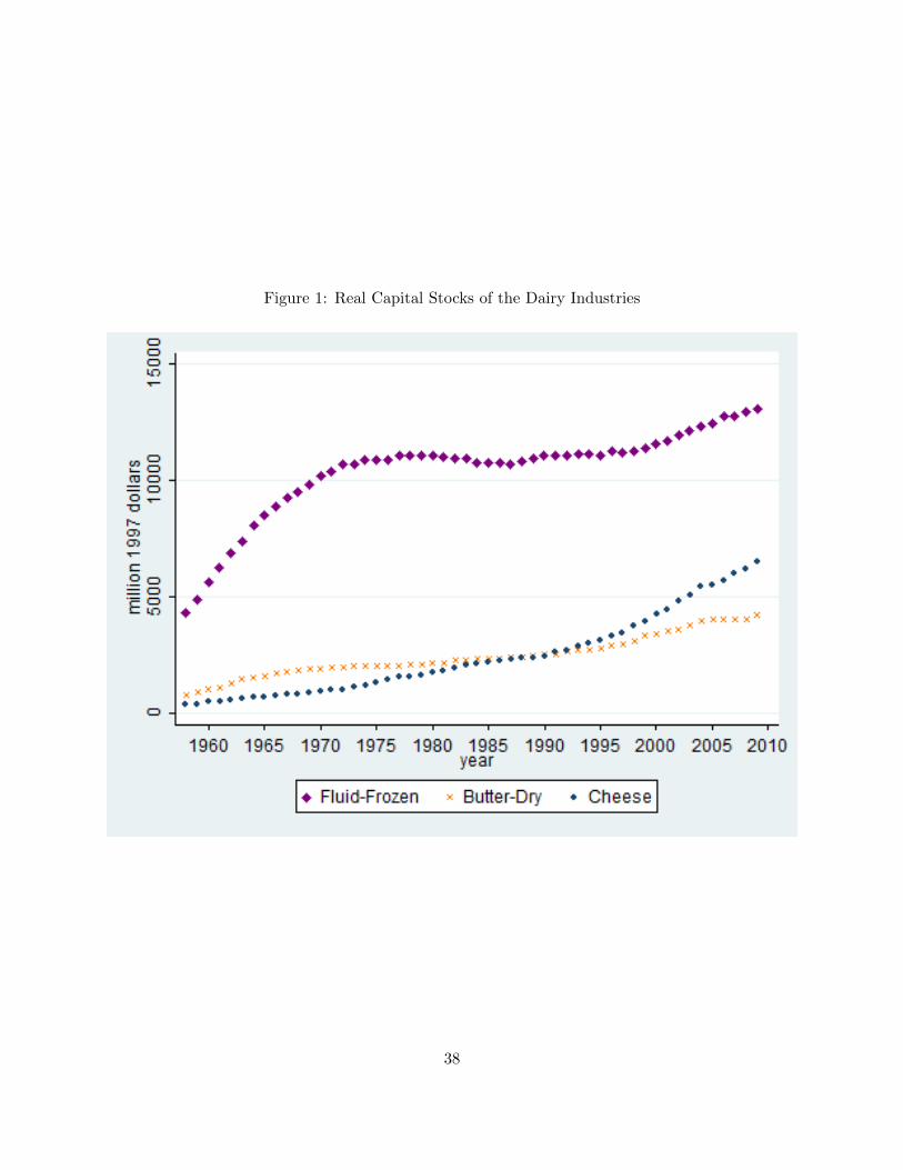
First, we constructed a measure of capital expenditure using data in the NBER database on capital
stocks. The NBER database includes data on real capital stocks of equipment and structures,
which are constructed using the data on net capital stocks from the Federal Reserve Board (FRB)
(Bartelsman and Gray, 1996; Becker, Gray, and Marvakov, 2013). The FRB data on net capital
stock are constructed using a perpetual inventory model (Mohr and Gilber, 1996). Figure 1 plots
real capital stocks for the three dairy industries. The capital stock of the fluid-frozen dairy industry
is much larger than those of the other two industries.
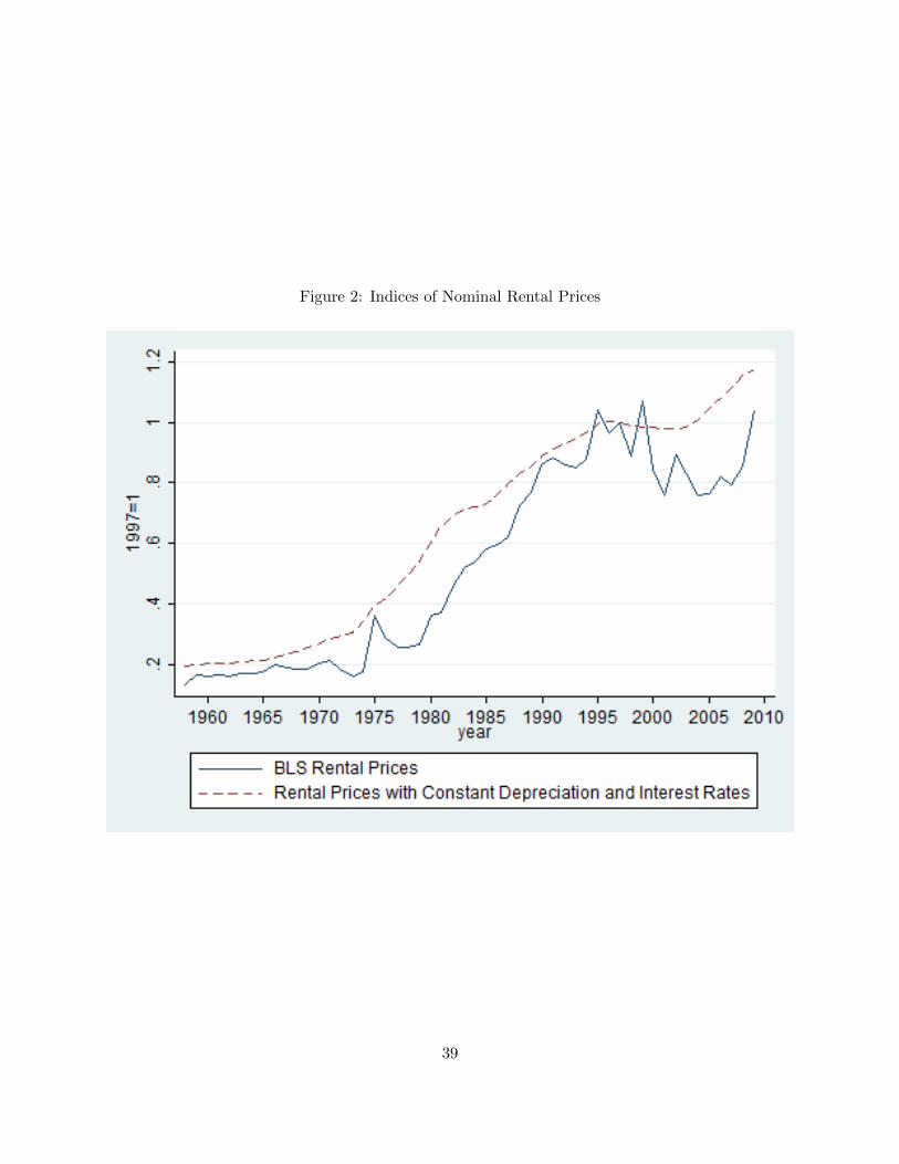
Estimates of nominal rental prices were obtained from the Bureau of Labor Statistics (BLS).
The BLS estimates of rental prices take account of the nominal rates of return to capital assets, the
nominal rates of economic depreciation, and revaluation of assets. Rental prices are also adjusted
for the effects of taxes (Bureau of Labor Statistics, 2006, 2007). In constructing the rental prices,
12
BLS computes an “internal rate of return,” it in equation (4), using data on property income taken
from the National Income Production Account (NIPA) (Jorgenson and Griliches, 1967). The BLS
assumed a hyperbolic depreciation pattern to compute δt, such that assets lose efficiency at a slow
rate early in their life and at a much faster rate as they age (Dean and Harper, 1998). We use the
estimates of the rental prices of structures and equipment for the food and beverage and tobacco
industry. Then, the rental price of capital is constructed as a weighted average of rental prices of
structures and equipment, using industry-specific structure and equipment stocks as weights.
In addition to using the rental prices from the BLS, we also considered constructing rental
rates under simplifying assumptions: 1) the rate of economic appreciation of new asset prices is
the same as the rate of general inflation, 2) a constant geometric rate of depreciation, and 3) a
constant real interest rate. Under these assumptions, equation (4) becomes ρt = Pt(r + δ), where
r is the real interest rate (equal to the nominal interest rate i minus the rate of general inflation).
Using an average service life of 25 years and assuming that an asset is retired when its productive
efficiency falls below 15%, we calculated that δ = 0.07.5 r is assumed to be 0.03. The NBER
database includes nominal price indices for new investment in equipment and structures (Pt). we
computed rental prices, ρt, according to ρt = Pt(r + δ).
Figure 2 plots nominal rental prices obtained from the BLS and those constructed under
the above simplifying assumptions. The two series trace each other relatively well, but the BLS
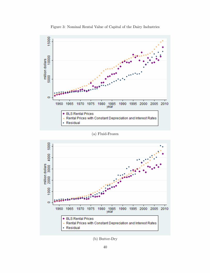
rental prices are more volatile. With the data on real capital stocks from the NBER database and
rental rates of capital either obtained from BLS or calculated by myself, we constructed measures
of capital service flows and rental expenditure. We also calculated capital rental expenditure as
the residual that exhausts the value of output. Figure 3 plots the three different measures of rental
expenditure for each dairy industry. For the butter-dry industry and the cheese industry, the
differences among the different measures of rental expenditure are relatively small. For the fluid-
frozen industry, the two measures of capital expenditure constructed using the NBER measure of
5The Bureau of Economic Analysis (BEA) uses geometric depreciation when estimating capital input. The meanservice life of equipment is assumed to be 20 years for the food industry (NAICS: 311) and the mean service life ofstructures for manufacturing industry is assumed to be 31 years (Bureau of Labor Statistics, 2006). BEA estimatesthe geometric depreciation rates by dividing “declining balance” parameters by estimates of the service lives of assets.The “declining balance” parameters used by BEA are respectively 1.65 for equipment and 0.91 for structures (Bureauof Labor Statistics, 2006). Thus, the depreciation rates for equipment and structure are respectively 0.08 and 0.03.
13
capital stock deviate significantly from the residual measure of capital expenditure. This is mainly
driven by the measure of capital stock of the fluid-frozen dairy industry in the NBER database.
In the estimation, we assume constant returns to scale and use as the rental expenditure
of capital the residual that exhausts the value of output. We estimated the models using both
measures of rental prices and the results are not qualitatively different. The reported results are
obtained using the BLS rental prices. Table 2 summarizes the cost shares of inputs for each industry
over the sample period. The cost shares of capital have been increasing, especially during the 1990s,
and the shares of labor have been decreasing, especially for the fluid-frozen dairy industry.
6 Empirical Implementation
This section first introduces the flexible functional forms that we use in econometric estimation,
and then investigates technical change using the growth accounting method. We summarize some
of the econometric results in the last subsection.
6.1 Functional Forms
We consider two locally flexible functional forms in the empirical analysis: the generalized Leontief
(GL) (Diewert, 1971) and the translog (Christensen, Jorgenson, and Lau, 1973). Locally flexible
functional forms provide a second-order approximation to an arbitrary twice continuously differen-
tiable function (see chapter 5 of Chambers (1988) for an introduction to flexible functional forms).
A GL cost function is a generalized version of a cost function based on a fixed proportions pro-
duction function. One advantage of the GL functional form is that it allows analytical imputation
of quasi-fixed input and thus is particularly useful for approximation of a restricted (variable) cost
function. The specific GL functional form used in this analysis was used by Morrison Paul (2001)
and Morrison Paul and MacDonald (2003).6 A translog form is an extension of the Cobb-Douglas
functional form; it is a second- instead of first- order log-linear function. One implication of the
translog functional form is that, since it is defined in logarithms, computations of some elasticities
6This particular GL functional form is referred to as a generalized Leontief-quadratic form by Morrison Paul(2001). Unlike a traditional GL functional form, this form allows zero values for inputs and outputs.
14
depend only on the parameter estimates rather than being a function of data. Neither of the func-
tional forms imposes curvature conditions directly. Violations can be checked at each data point
(Gallant and Golub, 1984). The GL form tends empirically to generate fewer curvature violations
than the translog in a model of restricted cost function (Morrison Paul, 1999, Chapter 11). Caves
and Christensen (1980) have shown that the GL has satisfactory local properties when substitution
among inputs is low.
Under the maintained assumption of constant returns to scale, the average cost function
for the GL functional form is specified as equation (6).
C(w, t) =∑i
βiIi +∑i
Ii∑j
βijwj +∑j
∑k
βjkw12j w
12k + t
∑i
Ii∑j
βijtwj + βttt2∑j
wj .(6)
Subscripts j and k denote inputs, and Ii with i ∈ {1, 2, 3} denote the fluid-frozen, butter-dry,
and cheese industries respectively. We estimate the model using pooled data of the three dairy
industries. Industry dummy variables for intercepts are included in all of the estimating equations.
We also allow the coefficient of the time-trend variable to vary by industry to capture different rates
of technical change among the three industries. The other parameters, βjk, representing factor
demand relationships, are held constant for the three industries. Applying Shephard’s lemma to
equation (6) yields input-output demand equations, which are the demand functions for inputs per
unit of output for the GL model. For example, the input-output demand equation for energy is
(7)xEy
=∑i
βiEIi +∑k 6=E
βEkw12k w− 1
2E + t
∑i
βiEtIi + βttt2.
The average cost function for the translog functional form is specified as:
lnC(w, t) =∑i
αiIi +∑i
Ii∑j
αij lnwj + 12
∑j
∑k
αjk lnwj lnwk
+ t∑i
αitIi + t∑i
Ii∑j
αijt lnwj .
(8)
Applying Shephard’s lemma to equation (8) yields input cost share equations for the translog model.
15
For example, the energy share equation is
(9) sE =∑i
αiEIi +∑k
αEk lnwk + t∑i
αiEtIi.
When using a GL functional form, the estimating system consists of the average cost func-
tion and input-output demand equations for capital, labor, energy, milk, and other processing
materials. Linear homogeneity of the cost function in input prices is satisfied with this specific
GL functional form. When using a translog functional form, we estimate a system of equations
consisting of the average cost function and cost share equations. Linear homogeneity of the cost
function is accomplished by normalizing the average cost and the prices of capital, labor, energy,
and milk by the price of other materials.
6.2 Growth Accounting
Before estimating the cost function model, we investigate technical change using a growth account-
ing method. Growth accounting was first suggested by Solow (1957). The underlying idea of growth
accounting with a cost function is that the changes in the cost of production after accounting for
changes in output quantity and input prices—the residual—can be attributed to technical change.
Specifically,
(10)d lnTC
d t=
d lnQ
d t+∑j
12(sjt−1 + sjt)
d lnwj
d t+ residual,
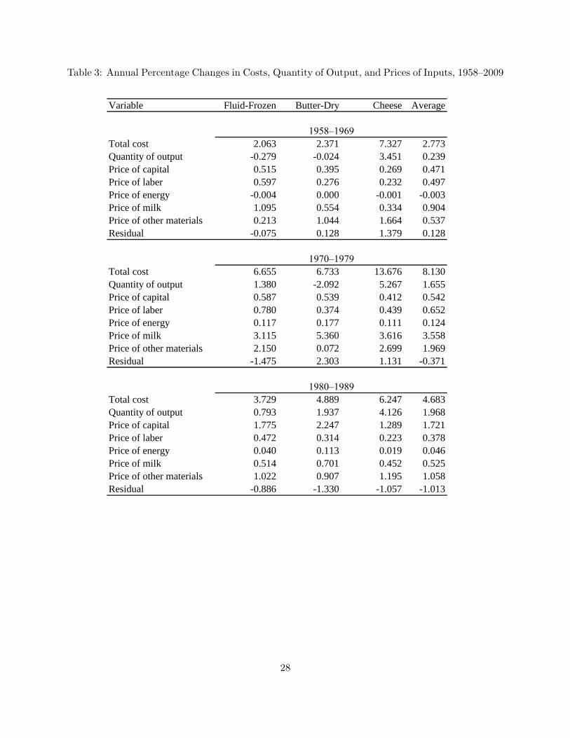
where sjt is the total cost share of input j in year t. Table (3) presents the annual percentage
changes in the total cost of production, output quantity, and the share-weighted changes in input
prices for each dairy industry. Residuals are calculated according to equation (10). The residuals
are generally small. Negative residuals can be seen for all three dairy industries during the 1980s
and the 2000s, with annual average 1% reductions in costs of production during the two decades.
However, this residual measure may embody other effects on the cost of production, such as changes
in output composition, and input and output quality, as well as technical progress.
16
6.3 Results
We first estimate the econometric models using seemingly unrelated regressions (SUR). In addition
to linear homogeneity, symmetry of the Hessian matrix is imposed. The majority of the parameter
estimates are statistically significant. Parameter estimates that are not individually statistically
significant are jointly significant. See Appendix A for details.
Table 4 presents the price elasticities of factor demand at the mean of sample data for each
dairy industry. Standard errors are in parentheses. Elasticity estimates are nonlinear functions
of model parameters, so the standard errors are obtained by applying the bootstrap method with
replacement for 1,000 iterations (Eakin, McMillen, and Buono, 1990; Krinsky and Robb, 1991).
Most of the estimates are statistically significant, except for some of the estimates related to energy.
The estimates from the two functional forms generally differ, but most of them are similar such
that the economic implications of the two models are the same.
For the fluid-frozen dairy industry, the GL estimates of the own-price elasticities of demand
for capital, labor, energy, milk, and other processing materials are respectively -0.50,-0.30, -0.24,
-0.10, and -0.37. The corresponding estimates from the translog specification are all larger in
magnitude, especially for labor and energy, but are all inelastic. For the butter-dry industry,
the GL estimates of the own-price elasticities of demand for capital, labor, energy, milk, and
other processing materials are respectively -0.47,-0.67, -0.20, -0.09, and -0.62. The corresponding
estimates from the translog specification are similar, except that the demand for energy is estimated
to be more elastic, with an own-price elasticity of −0.73. Estimates from the two functional forms
differ the most for the cheese industry. The own-price elasticities of demand for capital, labor,
energy, milk, and other processing materials are respectively −0.83,−0.67,−0.30,−0.10, and −0.28
from the GL specification, and are respectively −0.43,−0.41,−0.61,−0.16, and −0.44 from the
translog specification. In summary, the demands for inputs by the dairy industries are all inelastic.
The estimates indicate that the own-price elasticity of demand for capital is between −0.43 and
−0.83, for labor is between −0.30 and −0.67, for energy is between −0.20 and −0.73, for milk is
between −0.09 and −0.16, and for other processing materials is between −0.28 and −0.62. The
demand for milk is the least elastic. The cost share of milk averaged 0.32 to 0.61 over the sample
17
period for the three dairy industries.
The estimates of the cross-price elasticities vary across industries, but imply similar sub-
stitute or complementary relationships. Capital and energy are estimated to be used in fixed
proportions, except that they may be complements in the production of cheese. Labor and energy
are estimated to be complements, but the estimates of the cross-price elasticities between labor and
energy are not statistically significantly different from zero. Estimates from both functional forms
imply that milk and energy, and materials and energy are substitutes, but only the estimates from
the translog specification are statistically significant. Based on the estimates from the translog
specification, a 10% increase in the price of energy would lead to a 0.3% decrease in the demand
for milk, and a 0.1% decrease in the demand for other processing materials. Across other factors,
capital and materials are estimated to be substitutes for labor and milk, and each other, except that
capital may be a complement for milk in the production of cheese; labor and milk are estimated to
be complements. A 10% increase in the price of milk would lead to a 2–5% decrease in the demand
for labor, and a 1–2% increase in the demand for other processing materials.
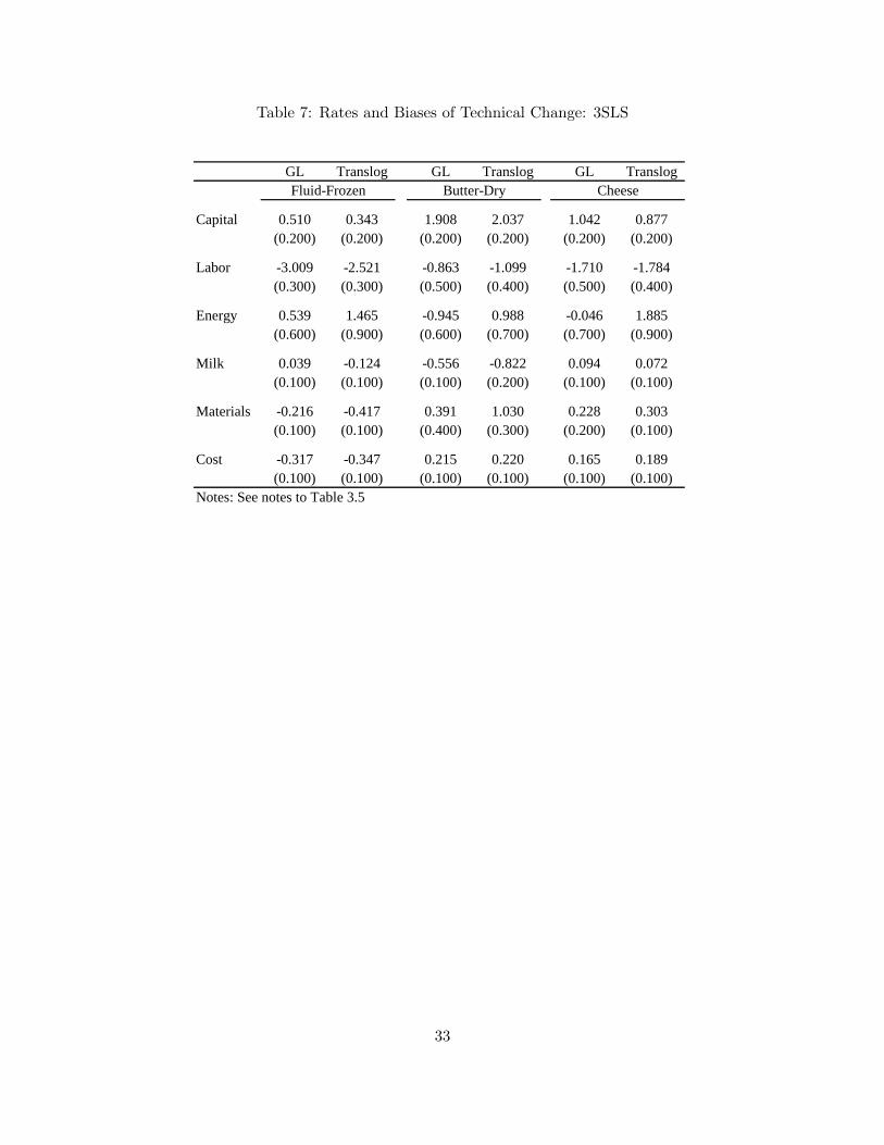
Table 5 summarizes the elasticities of the average cost and input demands with respect
to the time-trend variable. The dairy processing and manufacturing industries did not experience
much technical progress in the sample period, indicated by the small estimates of ηCt. This result is
also supported by the growth accounting exercise conducted above. Estimates from both functional
forms imply that technical change has been capital-using and labor-saving for all three industries,
which is very plausible given the movements of the relative price of capital to labor. To put the
estimates into perspective, we calculate the term ηjt − ηCt in the definition of technical change
bias, which measures the relative change in the cost shares of factors holding factor prices constant.
The cost share of capital increased by 0.7% per year for the fluid-frozen industry and the cheese
industry, and by 1.8% per year for the butter-dry industry. The cost share of labor decreased by
about 2.0% per year for the fluid-frozen and the cheese industry, and about 1.0% for the butter-dry
industry. For the other inputs, biases of technical change are relatively small. Estimates from the
GL specification indicate that technical change has been energy-using for fluid-frozen industry, and
energy-saving for butter-dry and for cheese manufacturing, but none of the estimates is statistically
18
significant at a reasonable level. The translog specification indicates that technical change has been
energy-using for all three dairy industries, and statistically significant for cheese manufacturing.
The cost share of energy has been increasing by 1.7% per year for the cheese industry.
7 Robustness Checks
In addition to the estimates reported in the previous section, we also conducted instrumental-
variable estimation of the models, and considered short-run capital fixity. This section summarizes
some of the results for robustness checks.
7.1 Instrumental Variable Estimation
As mentioned in section 2, we are not particularly concerned with the endogeneity of explanatory
variables in this analysis, since the dairy processing and manufacturing industry is not a significant
player in the markets of most of its inputs and the price of farm milk is established by milk marketing
orders. For a robustness check, we provide estimates of the elasticities from instrumental-variable
estimation using three-state least squares (3SLS). We use a set of instrumental variables: the price of
corn, cow inventory per capita, population, gross domestic product per capita, corporate income tax
rate, personal labor income tax rate, and the price of oil. We also estimated the model with various
sets of instruments, but the elasticity estimates are closely similar across different combinations of
instruments. Table (6) summarizes the estimated price elasticities of factor demand at the mean of
the data for each of the three dairy processing and manufacturing industries and Table (7) presents
the estimates of the elasticities of the average cost and input demands with respect to the time-
trend variable. Comparing the estimates from Table (6) and Table (4), and from Table (7) and
Table (5), none of the estimates is qualitatively different from the SUR estimates.
7.2 Capital Fixity
A cost model should be specified in terms of true economic value. If markets are working perfectly,
market price is an appropriate estimate of the economic value of an input. When it is not the
case, shadow values should be used. When short-run fixity of capital causes a deviation between its
19
market price and economic value, and hence a violation of Shephard’s lemma, it is more appropriate
to incorporate capital quantity into a cost function and to include an implicit optimization equation
of capital in the estimation system (Morrison, 1988; Chun and Nadiri, 2008).
With capital fixity taken into consideration, the (restricted) average cost function of the GL
functional form is specified as equation (11) and the input-output demand for energy is specified
as equation (12).
C =∑i
βiIi +∑i
Ii∑j
βijwj +∑j
∑k
βjkw12j w
12k + +xK
∑i
βiKIi∑j
wj
+ t∑i
Ii∑j
βijtwj + (βttt2 + βKKx
2K + βtKtxK)
∑j
wj ,
(11)
xEy
=∑i
βiEIi +∑k 6=E
βEkw12k w− 1
2E + xK
∑i
βiKIi + t∑i
βiEtIi + βttt2 + βKKx
2K + βtKtxK .(12)
At equilibrium, the optimal quantity of capital services is determined by the condition that the
rental rate of capital is equal to the magnitude of the reduction in variable cost resulting from
an additional unit of capital input. Using wK to denote the rental rate of capital, this condition
implies that wK = − ∂C∂xK
in equilibrium. When using a GL functional form, the equilibrium
condition implies the estimating equation (13):
(13) −wK =∑i
βiKIi∑j
wj + (2βKKxK + βtKt)∑j
wj .
Similarly, the restricted cost function of the translog functional form is specified as equation
(14), the cost share of energy is specified as equation (15), and the equilibrium condition for capital
20
input is equation (16):
lnC =∑i
αiIi +∑i
Ii∑j
αij lnwj + 12
∑j
∑k
αjk lnwj lnwk
+ lnxK∑i
αiKIi + lnxK∑j
αjK lnwj + t∑i
αitIi
+ t∑i
Ii∑j
αijt lnwj + t lnxK∑i
αiKtIi + 12αKK(lnxK)2 + 1
2αttt2,
(14)
sE =∑i
αiEIi +∑k
αEk lnwk + αEK lnxK + t∑i
αiEtIi,(15)
−sK =∑i
αiKIi +∑j
αjK lnwj + αKK lnxK + t∑i
αiKtIi.(16)
Table 8 summarizes the GL estimates of the cross-price elasticities in the short run (SR)
when the quantity of capital service is fixed and in the long run (LR) when capital input can change.
These estimates are calculated at the mean of the sample data for each of the three industries. The
LR demands for inputs other than labor are more elastic than what the estimates implied when
we assume instantaneous adjustment of capital. The signs of the elasticities indicating whether
inputs are substitutes or complements remain the same as those estimated assuming no capital
fixity. However, the precision of the estimates is lower compared with the estimates in Table 4.
The translog estimates of the cross-price elasticities in Table 9 also imply that the LR demands
for inputs are more elastic, except for labor. Moreover, in the LR, capital is estimated to be a
complement for energy, and the estimates imply that a 10% increase in the price of energy would
lead to a 0.4% decrease and a 0.8% decrease respectively in the demand for capital in fluid-frozen
and cheese manufacturing; labor, milk, and other materials are estimated to be substitutes for
energy, but most of the estimates are relatively small.
Table 10 summarizes the GL and translog estimates of the SR and LR elasticities of the
average cost and input demands with respect to the time-trend variable. The estimates indicate that
the average cost of manufacturing fluid-frozen and butter-dry dairy products has been decreasing by
respectively about 1% and 0.5% per year. Estimates from both functional forms imply that technical
change has been capital-using and labor-saving for all three industries and the LR estimates are
21
larger in magnitude in comparison to the estimates obtained assuming instantaneous adjustment
of capital. In the LR, the cost share of capital has been increasing by 2–4% per year for the dairy
industries, and the cost share of labor has been decreasing by about 2.5% per year for the fluid-
frozen and the cheese industries, and about 1.0% for the butter-dry industry. For the other inputs,
biases of technical change are relative small.
8 A Discussion of Derived Demand for Farm Milk
In addition to assessing the substitution between energy and other inputs, estimation results from
this paper can also be used to characterize the demand for farm milk. The demand for farm
milk is not a consumer demand, but rather a derived demand for an input used by the dairy
processing and manufacturing industry. Therefore, estimates of the price elasticities of demand
for dairy products are not directly comparable to estimates of the price elasticity of demand for
farm milk. Moreover, a fixed relationship does not exit between the price elasticities of demand
for final products and the elasticities of derived demand for factors (Wohlgenant, 1989, 2001).
However, under the assumptions that the production technology exhibits constant returns to scale
and the output markets are perfectly competitive, the relationship defined in equation (17) between
the price elasticity of derived demand for milk and price elasticities of demand for the three final
products holds:
(17) η1MM = η̃1MM + η1s1M + η12s2M + η13s3M ,
where η1MM denotes the Marshallian own-price elasticity of demand for milk used in product 1,
η̃1MM is the Hicksian (output-constant) own-price elasticity of demand for milk used in product 1,
η1 is the own-price elasticity of demand for product 1, η12 and η13 are the elasticities of demand
for product 1 with respect to the prices of product 2 and 3 respectively, and s1M , s2M , and s3M are
the shares of milk in the cost of producing products 1, 2, and 3. Similar relationships hold for η2MM
and η3MM .
By estimating the factor demand relationship of the dairy processing and manufacturing
22
dairy industry, we have estimated the output-constant own-price elasticities of demand for farm
milk for the three dairy industries analyzed in this paper—fluid-frozen, cheese, and butter-dry.
Using equation (17), we can obtain “synthetic” estimates of Marshallian own-price elasticity of
demand for farm milk. We use the estimates of output-constant elasticities reported in Table 4 to
calculate the Marshallian elasticity of derived demand for milk. Estimates of the price elasticities
of demand for dairy products are obtained from the literature. Only studies of the U.S. consumers
are considered. Published estimates of the own-price elasticity of retail demand range from −0.652
to −0.039 for fluid milk (Huang, 1993; Schmit and Kaiser, 2004; Chouinard et al., 2010), and range
from −0.741 to −0.078 for other dairy products (Huang, 1993). We use −0.20, −0.50, and −0.60
as the estimates of the own-price elasticity of demand for fluid-frozen, cheese, and butter-dry dairy
products respectively. Cross-price elasticities of demand for different dairy products are small.
Huang (1993) estimated cross-price elasticities among dairy products. The elasticity of fluid milk
consumption with respect to the prices of cheese, evaporated and dry milk, butter, and frozen dairy
products are respectively 0.008,−0.060, 0.021, and −0.032. We use 0.02 as an estimate of all the
cross-price elasticities of demand for dairy products. Balagtas and Kim (2007) used a similar set
of estimates in their analysis.
We use the average cost shares of milk for the years 2005–2009 to calculate the elasticities
of derived demand for milk. Table 11 presents the results. We calculate the elasticities of derived
demand for milk using both the GL and the tranlog estimates of the output-constant own-price
elasticities of demand for milk. The calculated Marshallian own-price elasticity of demand for milk
is between −0.14 and −0.20 for the fluid-frozen dairy products, between −0.31 and −0.37 for the
buttery-dry dairy products, and between −0.26 and −0.31 for cheese. The aggregate elasticity of
derived demand for milk can be calculated as follows,
(18) ηMM = θ1Mη1MM + θ2Mη
2MM + θ3Mη
3MM ,
where θ1M , θ2M , and θ3M represent the shares of milk used for industry 1, 2, and 3. The aggregate
elasticity of derived demand for milk is calculated using the average shares of milk used for the final
products for the years 2005–2009, which are also reported in Table 11. In aggregate, the own-price
23
elasticity of demand for farm milk is between −0.22 and −0.28. Given that we use estimates of the
own-price elasticities of demand for dairy products from the literature to calculate the elasticities
of derived demand for milk, the reliability of these synthetic estimates depends partially on the
quality of the studies from which some estimates were drawn. Future research may involve a
thorough meta-analysis of the studies on the demand for dairy products, so that We can calculate
confidence levels for these synthetic estimates of the own-price elasticity of demand for farm milk,
or a new estimate of those elasticities.
9 Conclusion
This paper studies the cost structure and the input demand relationships of the dairy processing
and manufacturing industry in the United States, with a focus on the substitution between energy
and other inputs, and the rate and biases of technical change.
The cross-price elasticities between other inputs and energy are generally small. When
assuming instantaneous adjustment of capital, estimates of the cross-prices elasticities indicate
that capital and energy are used in fixed proportions, labor is complement for energy, and milk
and other materials are substitutes for energy. When allowing for short-run capital fixity, the LR
estimates from the GL functional form also imply that labor and energy are complements, but the
translog estimates imply a fixed-proportions relationship between labor and energy in the long run.
The LR estimates from the translog functional form imply some weak complementarity between
capital and energy in fluid-frozen and cheese manufacturing. Milk and other materials are estimated
to be substitutes for energy, but only the estimates from the translog specification are statistically
significant.
The estimated rate of technical change is small, implying that technical change is not a
driving force in altering the cost structure of the dairy industry. Estimates from both model
specifications imply that technical change of the dairy industry has been capital-using and labor-
saving. The cost share of capital has been increasing by about 1-4% per year and the cost share of
labor has been decreasing by about 2% per year. For other factors, biases of technical change are
relatively small.
24
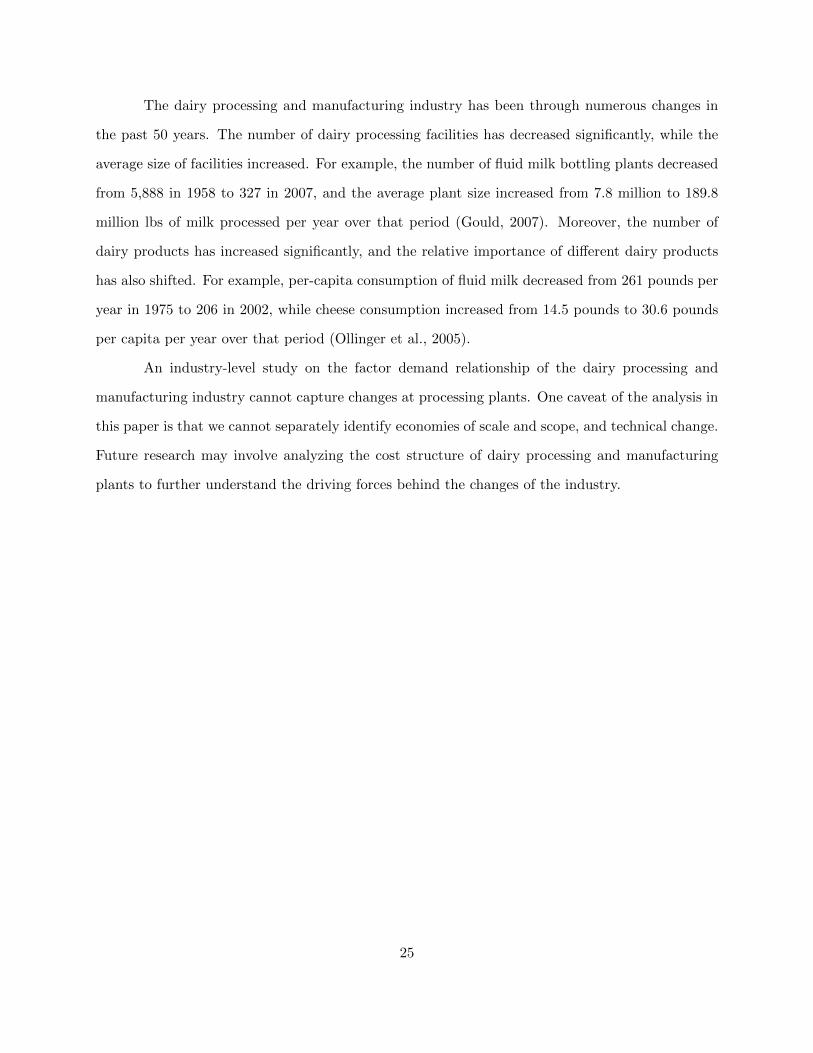
The dairy processing and manufacturing industry has been through numerous changes in
the past 50 years. The number of dairy processing facilities has decreased significantly, while the
average size of facilities increased. For example, the number of fluid milk bottling plants decreased
from 5,888 in 1958 to 327 in 2007, and the average plant size increased from 7.8 million to 189.8
million lbs of milk processed per year over that period (Gould, 2007). Moreover, the number of
dairy products has increased significantly, and the relative importance of different dairy products
has also shifted. For example, per-capita consumption of fluid milk decreased from 261 pounds per
year in 1975 to 206 in 2002, while cheese consumption increased from 14.5 pounds to 30.6 pounds
per capita per year over that period (Ollinger et al., 2005).
An industry-level study on the factor demand relationship of the dairy processing and
manufacturing industry cannot capture changes at processing plants. One caveat of the analysis in
this paper is that we cannot separately identify economies of scale and scope, and technical change.
Future research may involve analyzing the cost structure of dairy processing and manufacturing
plants to further understand the driving forces behind the changes of the industry.
25
Table 1: A List of Dairy Processors and Manufacturers in California
Handler ID County
Fluid and Soft Butter Cheese Dry Frozen
92135 Sonoma * *
148312 Los Angeles *
148576 Los Angeles *
14211 Alameda *
92102 Sonoma
11538 Alameda *
80006 Del Norte *
32075 Tulare *
142097 Los Angeles *
12033 Contra Costa *
148390 Los Angeles * *
143175 San Luis Obispo * *
37058 Fresno * * *
146013 Los Angeles *
41062 Merced * *
35045 Tulare *
76064 Stanislaus * * *
36090 Tulare * * *
36068 Tulare * * *
32119 Fresno * * * *
73370 Stanislaus * *
12396 San Benito *
93015 Sonoma *
42041 Stanislaus *
80010 Kings *
142560 Los Angeles * * *
148400 Orange *
142020 Orange *
142152 Riverside *
35034 Kern *
35012 Tulare *
141371 Los Angeles * *
42020 Kings *
78330 Kings *
18039 Alameda *
144210 Los Angeles *
35023 Fresno * *
74095 Stanislaus * * * *
28050 Humboldt * *
140492 Los Angeles *
145210 Los Angeles *
Types of Products
Source: Author's summerization based on CDFA (2011). "Fluid and Soft" products include fluid milk,
buttermilk, cottage cheese, cream, eggnog, sour cream, and yogurt. "Dry" products include condensed and
evaporated milk, whey protein concentrates, and nonfat dry milk.
26
Table 2: Cost Shares of Inputs of the U.S. Dairy Industries, 1958–2009
Variable Fluid-Frozen Butter-Dry Cheese Average
Capital 0.175 0.143 0.089 0.160
Labor 0.146 0.061 0.065 0.122
Energy 0.009 0.014 0.009 0.010
Milk 0.384 0.607 0.436 0.429
Other Materials 0.286 0.175 0.400 0.279
Capital 0.160 0.166 0.103 0.148
Labor 0.106 0.052 0.051 0.086
Energy 0.009 0.013 0.008 0.010
Milk 0.437 0.585 0.396 0.451
Other Materials 0.288 0.184 0.442 0.305
Capital 0.171 0.233 0.133 0.171
Labor 0.085 0.051 0.048 0.069
Energy 0.014 0.015 0.012 0.014
Milk 0.418 0.508 0.424 0.434
Other Materials 0.312 0.193 0.384 0.312
Capital 0.214 0.336 0.164 0.217
Labor 0.087 0.061 0.048 0.070
Energy 0.012 0.012 0.009 0.011
Milk 0.377 0.387 0.342 0.366
Other Materials 0.310 0.204 0.436 0.336
Capital 0.290 0.334 0.158 0.251
Labor 0.085 0.058 0.054 0.070
Energy 0.012 0.016 0.012 0.013
Milk 0.321 0.358 0.343 0.334
Other Materials 0.293 0.234 0.433 0.333
Capital 0.201 0.238 0.128 0.189
Labor 0.104 0.057 0.054 0.083
Energy 0.011 0.014 0.010 0.011
Milk 0.387 0.494 0.390 0.406
Other Materials 0.297 0.197 0.418 0.311
Notes: Average shares of the three industries are weighted by the industry share
of nominal output.
1958–1969
1970–1979
1980–1989
1990–1999
2000–2009
1958–2009
27
Table 3: Annual Percentage Changes in Costs, Quantity of Output, and Prices of Inputs, 1958–2009
Variable Fluid-Frozen Butter-Dry Cheese Average
Total cost 2.063 2.371 7.327 2.773
Quantity of output -0.279 -0.024 3.451 0.239
Price of capital 0.515 0.395 0.269 0.471
Price of laber 0.597 0.276 0.232 0.497
Price of energy -0.004 0.000 -0.001 -0.003
Price of milk 1.095 0.554 0.334 0.904
Price of other materials 0.213 1.044 1.664 0.537
Residual -0.075 0.128 1.379 0.128
Total cost 6.655 6.733 13.676 8.130
Quantity of output 1.380 -2.092 5.267 1.655
Price of capital 0.587 0.539 0.412 0.542
Price of laber 0.780 0.374 0.439 0.652
Price of energy 0.117 0.177 0.111 0.124
Price of milk 3.115 5.360 3.616 3.558
Price of other materials 2.150 0.072 2.699 1.969
Residual -1.475 2.303 1.131 -0.371
Total cost 3.729 4.889 6.247 4.683
Quantity of output 0.793 1.937 4.126 1.968
Price of capital 1.775 2.247 1.289 1.721
Price of laber 0.472 0.314 0.223 0.378
Price of energy 0.040 0.113 0.019 0.046
Price of milk 0.514 0.701 0.452 0.525
Price of other materials 1.022 0.907 1.195 1.058
Residual -0.886 -1.330 -1.057 -1.013
1958–1969
1970–1979
1980–1989
28
Table 3: Annual Percentage Changes in Costs, Quantity of Output, and Prices of Inputs, 1958–2009(Continued)
Variable Fluid-Frozen Butter-Dry Cheese Average
Total cost 1.043 3.179 4.372 2.565
Quantity of output -1.541 0.998 2.558 0.300
Price of capital 0.694 1.090 0.515 0.696
Price of laber 0.250 0.135 0.161 0.201
Price of energy 0.018 0.017 0.012 0.016
Price of milk 0.370 0.015 0.033 0.195
Price of other materials 0.009 0.482 0.439 0.234
Residual 1.243 0.443 0.653 0.923
Total cost 3.018 3.375 3.156 3.234
Quantity of output 1.736 2.736 3.381 2.562
Price of capital 0.004 -0.211 -0.197 -0.116
Price of laber 0.312 0.237 0.177 0.252
Price of energy 0.020 0.043 0.031 0.027
Price of milk -0.318 -0.315 -0.114 -0.252
Price of other materials 1.833 1.654 1.503 1.702
Residual -0.569 -0.769 -1.624 -0.942
Total cost 3.277 4.075 6.963 2.581
Quantity of output 0.404 0.696 3.751 0.350
Price of capital 0.711 0.804 0.454 0.547
Price of laber 0.485 0.267 0.246 0.326
Price of energy 0.037 0.068 0.034 0.033
Price of milk 0.958 1.249 0.854 0.764
Price of other materials 1.029 0.836 1.503 0.736
Residual -0.347 0.155 0.122 -0.176
Notes: Average changes of the three industries are weighted by the industry share
of nominal output.
1958–2009
2000–2009
1990–1999
29
Table 4: Output-Constant Price Elasticities of Factor Demand
Capital Labor Energy Milk Materials Capital Labor Energy Milk Materials