Factorial Schur Functions and theYang-Baxter Equation

Daniel Bump, Peter J. McNamara and Maki Nakasuji

May 29, 2014

Abstract. Factorial Schur functions are generalizations of Schur functions that have, in

addition to the usual variables, a second family of “shift” parameters. We show that a

factorial Schur function times a deformation of the Weyl denominator may be expressed

as the partition function of a particular statistical-mechanical system (six-vertex model).

The proof is based on the Yang-Baxter equation. There is a deformation parameter t

which may be specialized in different ways. If t = −1, then we recover the expression of

the factorial Schur function as a ratio of alternating polynomials. If t = 0, we recover

the description as a sum over tableaux. If t = ∞ we recover a description of Lascoux

that was previously considered by the second author. We also are able to prove using the

Yang-Baxter equation the asymptotic symmetry of the factorial Schur functions in the

shift parameters. Finally, we give a proof using our methods of the dual Cauchy identity

for factorial Schur functions. Thus using our methods we are able to give thematic proofs

of many of the properties of factorial Schur functions.

Dedicated to Professor Fumihiro Sato

1 Introduction

Factorial Schur functions are generalizations of ordinary Schur functionssλ(z) = sλ(z1, · · · , zn) for which a surprising amount of the classical theoryremains valid. In addition to the usual spectral parameters z = (z1, · · · , zn)and the partition λ they involve a set α = (α1, α2, α3, · · · ) of shifts that canbe arbitrary complex numbers (or formal variables), and are denoted sλ(z|α).In the original paper of Biedenharn and Louck [BL], only the special casewhere αn = 1 − n was considered. Their motivation, inspired by questions

1

from mathematical physics, was to the decomposition of tensor products ofrepresentations with using particular bases. It turns out that factorial Schurfunctions are the same as double Schubert polynomials for Grassmannianpermutations, and in this form they appeared even earlier in Lascoux andSchutzenberger [LS1], whose motivation (from algebraic geometry) was com-pletely different.

Other early foundational papers are Chen and Louck [CL], who gavenew foundations based on divided difference operators, and Goulden andHamel [GH] where the analogy between Schur functions and factorial Schurfunctions was further developed. In particular they gave a Jacobi-Trudiidentity. See Louck [Lou] for further historical remarks.

Biedenharn and Louck (in the special case αn = 1 − n) defined sλ(z|α)to be a sum over Gelfand-Tsetlin patterns, and this definition extends tothe general case. Translated into the equivalent language of tableaux, theirdefinition is equivalent to (14) below. It was noticed independently by Mac-donald [Mcd1] and by Goulden and Greene [GG] that one could generalizethe factorial Schur functions of Biedenharn and Louck by making use of anarbitrary set α of shifts. Macdonald observed an alternative definition of thefactorial Schur functions as a ratio of two alternating polynomials, general-izing the Weyl character formula. This definition is (7) below.

Both Macdonald and Goulden and Greene also noticed a relationshipwith what are called supersymmetric Schur functions . These are symmetricfunctions in two sets of variables, z = (z1, z2, · · · ) and w = (w1, w2, · · · ).They are defined in terms of the ordinary Schur functions by

sλ(z‖w) =∑µ,ν

cλµν sµ(z)sν′(w),

where cλµν is the Littlewood-Richardson coefficient, µ and ν run throughpartitions and ν ′ is the conjugate partition. The relationship between thefactorial Schur functions and the supersymmetric Schur functions is this:although the sλ(z|α) are symmetric in the zi they are not symmetric in theαi. Nevertheless, as the number n of the parameters zi tends to infinity, theybecome symmetric in the αi in a certain precise sense, and in the limit, theystabilize. Thus in a suitable sense

limn−→∞

sλ(z|α) = sλ(z‖α). (1)

Another important variant of the factorial Schur functions are the shiftedSchur functions that were proposed by Olshanskii, and developed by Ok-

2

ounkov and Olshanskii [OO2], [OO1]. Denoted s∗λ(x1, · · · , xn), they are es-sentially the same as the factorial Schur functions of Biedenharn and Louck,but incorporate shifts in the parameters so that they are no longer symmetricin the usual sense, but at least satisfy the stability property s∗λ(x1, · · · , xn) =s∗λ(x1, · · · , xn, 0). These were applied to the representation theory of theinfinite symmetric group.

Molev and Sagan [MS] give various useful results for factorial Schurfunctions, including a Littlewood-Richardson rule. A further Littlewood-Richardson rule was found by Kreiman [Kr]. Knutson and Tao [KT] showthat factorial Schur functions correspond to Schubert classes in the equiv-ariant cohomology of Grassmanians. See also Mihalcea [Mi] and Ikeda andNaruse [IN].

Tokuyama [To] gave a formula for Schur functions that depends on aparameter t. This formula may be regarded as a deformation of the Weylcharacter formula. It was shown by Hamel and King [HK] that Tokuyama’sformula could be generalized and reformulated as the evaluation of the par-tition function for a statistical system based on the six-vertex model in thefree-fermionic regime. Brubaker, Bump and Friedberg [BBF] gave furthergeneralizations of the results of Hamel and King, with new proofs based onthe Yang-Baxter equation. More specifically, they used the fact that thesix-vertex model in the free-fermionic regime satisfies a parametrized Yang-Baxter equation with nonabelian parameter group GL(2) × GL(1) to givestatistical-mechanical systems whose partition functions were Schur func-tions times a deformation of the Weyl denominator. This result generalizesthe results of Tokuyama and of Hamel and King.

Our main new result (Theorem 1) is a Tokuyama-like formula for factorialSchur functions. This is a simultaneous generalization of [BBF] and of therepresentations of Lascoux [La2] and of McNamara [McN]. As in [BBF] wewill consider partition functions of statistical-mechanical systems in the free-fermionic regime. A significant difference between this paper and that wasthat in [BBF] the Boltzmann weights were constant along the rows, depend-ing mainly on the choice of a parameter zi. Now we will consider systems inwhich we assign a parameter zi to each row, but also a shift parameter αj toeach column. Furthermore, we will make use of a deformation parameter tthat applies to the entire system. We will show that the partition functionmay be expressed as the product of a factor (depending on t) that may berecognized as a deformation of the Weyl denominator, times the factorialSchur function sλ(z|α).

3

The proof of Theorem 1 depends on the Yang-Baxter equation. We feelthat it is significant that the Yang-Baxter equation can be made a centraltool in the theory of factorial Schur functions. The results in the paper afterTheorem 1 are mainly already known, but we will reprove them using ourmethods—either deducing them from Theorem 1 or giving proofs using thesame tool (free-fermionic Yang-Baxter equation).

By specializing t in the formula of Theorem 1, we will obtain differentformulas for the factorial Schur functions. Taking t = −1, we obtain therepresentation as a ratio of alternating polynomials, which was Macdonald’sgeneralization of the Weyl character formula. This is the formula we take asthe definition of the factorial Schur functions, though other definitions arepossible.

There are two specializations t in which the Weyl denominator in The-orem 1 reduces to a monomial. Taking t = 0, we obtain the tableau def-inition of the factorial Schur functions. When t = ∞ we recover anotherrepresentation of the factorial Schur functions. Indeed Lascoux [La2] foundsix-vertex model representations of Grassmannian Schubert polynomials. Aproof of this representation based on the Yang-Baxter equation was subse-quently found by McNamara [McN]. It is this representation that we obtainwhen t =∞.

Although we do not prove the supersymmetric limit (1), we will at leastprove the key fact that the sλ(z|α) are asymptotically symmetric in the αjas the number n of parameters zi tends to infinity. We will obtain this byanother application of the Yang-Baxter equation. We also give a proof of thedual Cauchy identity for factorial Schur functions using our methods.

In addition to [La2] and [McN], Zinn-Justin [ZJ1], [ZJ2] gave anotherinterpretation of factorial Schur functions as transition matrices for a latticemodel that may be translated into a free-fermionic five-vertex model. Itis unclear whether Zinn-Justin’s representation may also be obtained fromTheorem 1 ours by specialization, but it is certainly very similar.

We would like to thank H. Naruse for helpful comments on this paperand the referee for careful reading. This work was supported in part by JSPSResearch Fellowship for Young Scientists and by NSF grants DMS-0652817and DMS-1001079.

4

2 Yang-Baxter equation

We review the six-vertex model and a case of the Yang-Baxter equationfrom [BBF]. We will consider a planar graph. Each vertex v is assumed tohave exactly four edges adjacent to it. Interior edges adjoin two vertices, andaround the boundary of the graph we allow boundary edges that adjoin only asingle vertex. Every vertex has six numbers a1(v), a2(v), b1(v), b2(v), c1(v), c2(v)assigned to it. These are called the Boltzmann weights at the vertex. By aspin we mean an element of the two-element set {+,−}. In addition tothe graph, the Boltzmann weights at each vertex, we will also assign a spinto each boundary edge. Once we have specified the graph, the Boltzmannweights at the vertices, and the boundary spins, we have specified a statisticalsystem S.

A state s of the system will be an assignment of spins to the interioredges. Given a state of the system, every edge, boundary or interior, has aspin assigned to it. Then every vertex will have a definite configuration ofspins on its four adjacent edges, and we assume these to be in one of the twoorientations listed in (2). Then let βs(v) equal a1(v), a2(v), b1(v), b2(v), c1(v)or c2(v) depending on the configuration of spins on the adjacent edges. If vdoes not appear in the table, the weight is zero.

a1(v) a2(v) b1(v) b2(v) c1(v) c2(v)

(2)

The Boltzmann weight of the state β(s) is the product∏

v βs(v) of theBoltzmann weights at every vertex. We only need to consider configurationsin which the spins adjacent to each vertex are in one of the configurationsfrom the above table; if this is true, the state is called admissible. A statethat is not admissible has Boltzmann weight zero.

The partition function Z(S) is∑

s β(s), the sum of the Boltzmann weightsof the states. We may either include or exclude the inadmissible states fromthis sum, since they have Boltzmann weight zero.

5

If at the vertex v we have

a1(v)a2(v) + b1(v)b2(v)− c1(v)c2(v) = 0,

the vertex is called free-fermionic. We will only consider systems that arefree-fermionic at every vertex.

Korepin, Boguliubov and Izergin [KBI] describe a nonabelian parametrizedYang-Baxter equation for the free-fermionic six-vertex model with parametergroup Γ = SL(2,C). Concretely this means that there is a map R : Γ →End(V ⊗V ), where V is a two-dimensional vector space, such that if γ, δ ∈ Γthen

R(γ)12R(γδ)13R(δ)23 = R(δ)23R(γδ)13R(γ)12,

where if R ∈ End(V ⊗ V ) then Rij means R× IV acting on V ⊗ V ⊗ V withR acting on the i, j tensor components, and the identity on the remainingcomponent. Scalar matrices can obviously be added to Γ so their actualgroup is SL(2,C)×C×. A statement with a slightly larger parameter groupGL(2,C) × C× is in Brubaker, Bump and Friedberg [BBF]. The nonzerocomponents of R(γ) if written with respect to a standard basis of V ⊗V willbe the Boltzmann weights of a free-fermionic vertex. This has the followingexplicit reformulation:

Proposition 1. [BBF, Theorem 3] Let v, w be vertices with free-fermionicBoltzmann weights. Define another type of vertex u with

a1(u) = a1(v)a2(w) + b2(v)b1(w),

a2(u) = b1(v)b2(w) + a2(v)a1(w),

b1(u) = b1(v)a2(w)− a2(v)b1(w),

b2(u) = −a1(v)b2(w) + b2(v)a1(w),

c1(u) = c1(v)c2(w),

c2(u) = c2(v)c1(w).

Then for any assignment of edge spins εi ∈ {±} (i = 1, 2, 3, 4, 5, 6) the

6

following two configurations have the same partition function:

ε2

ε1

ν

µ

ε3

γ

ε6

ε4

ε5

u

v

w

δ

ψ

φ

ε2

ε1

ε3

ε6

ε4

ε5

w

v

u

. (3)

Note that by the definition of the partition function, the interior edgespins (labeled ν, γ, µ and δ, ψ, φ) are summed over, while the boundary edgespins, labeled εi are invariant. In order to obtain this from Theorem 3of [BBF] one replaces the R-matrix π(R) in the notation of that paper by aconstant multiple.

3 Bijections

In this section we will define some combinatorial bijections that we will needlater. One of the sets is the set of states of a statistical-mechanical system,as in the last section, and we start by defining that.

We will make use of two special n-tuples of integers, namely

ρ = (n, · · · , 3, 2, 1), δ = (n− 1, n− 2, · · · , 2, 1, 0).

Let λ = (λ1, · · · , λn) be a partition, so λ1 > . . . > λn > 0. Let us consider alattice with n rows and n+ λ1 columns. We will index the rows from 1 to n.We will index the columns from 1 to n + λ1, in reverse order . We put thevertex vΓ(i, j, t) at the vertex in the i row and j column.

We impose the following boundary edge spins. On the left and bottomboundaries, every edge is labeled +. On the right boundary, every edgeis labeled −. On the top, we label the edges indexed by elements of formλj + n − j + 1 for j = 1, 2, · · · , n with a − spin. These are the entries inλ+ ρ. The remaining columns we label with a + spin.

For example, suppose that n = 3 and that λ = (5, 4, 1), so λ+ρ = (8, 6, 2).Since λj +n− j+1 has the values 8, 6 and 2, we put − in these columns. We

7

label the vertex vΓ(i, j, t) in the i row and j column by ij as in the followingdiagram:

+

+

+

− + − + + + − +

+ + + + + + + +

−

−

−

1112131415161718

2122232425262728

3132333435363738

(4)

Let this system be called SΓλ,t.

We recall that a Gelfand-Tsetlin pattern is an array

T =

p11 p12 · · · p1n

p22 p2n

. . . . . .

pnn

(5)

in which the rows are interleaving partitions. The pattern is strict if eachrow is strongly dominant, meaning that pii > pi,i+1 > · · · > pin.

A staircase is a semistandard Young tableau of shape (λ1 + n, λ1 + n −1, . . . , λ1)′ filled with numbers from {1, 2, . . . , λ1 + n} with the additionalcondition that the diagonals are weakly decreasing in the south-east directionwhen written in the French notation.

An example of a staircase for λ = (5, 4, 1) is

8

7 8

6 7 8

5 6 6 7

4 5 5 5

3 3 3 4

2 2 2 3

1 1 1 1(6)

8

Proposition 2. Let λ be a partition of length 6 n. There are natural bijec-tions between the following three sets of combinatorial objects

1. States of the six-vertex model SΓλ,t,

2. Strict Gelfand-Tsetlin patterns with top row λ+ ρ, and

3. Staircases whose rightmost column consists of the integers between 1and λ1 + n that are not in λ+ ρ.

Proof. Suppose we start with a state of the six-vertex model SΓλ,t. Let us

record the locations of all minus spins that live on vertical edges. Betweenrows k and k+1, there are exactly n−k such minus spins for each k. Placingthe column numbers of the locations of these minus spins into a triangulararray gives a strict Gelfand-Tsetlin pattern with top row λ+ ρ.

Given a strict Gelfand-Tsetlin pattern T = (tij) with top row λ + ρ, weconstruct a staircase whose rightmost column is missing λ+ρ in the followingmanner: We fill column j + 1 with integers u1, . . . , un−j+λ1 such that

{1, 2, . . . , n+ λ1} = {u1, . . . , un−j+λ1} t {tn+1−j,1, . . . tn+1−j,j}.

It is easily checked that these maps give the desired bijections.

We give an example. As before let n = 3 and λ = (5, 4, 1). Here is anadmissible state:

+

+

+

+ − + + − + + +

− + − + + + − +

+ + + + − + + +

+ + + + + + + +

−

−

−

− + − − + + −

+ − − − − − −

+ + + + − − −

1112131415161718

2122232425262728

3132333435363738

Then the entries in the i-th row of T are to be the columns j in which a −appears above the (i, j) vertex. Therefore

T =

8 6 2

7 44

.

9

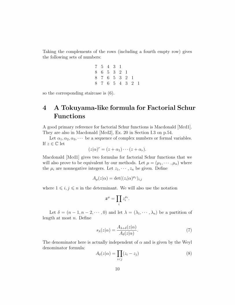
Taking the complements of the rows (including a fourth empty row) givesthe following sets of numbers:

7 5 4 3 18 6 5 3 2 18 7 6 5 3 2 18 7 6 5 4 3 2 1

so the corresponding staircase is (6).

4 A Tokuyama-like formula for Factorial Schur

Functions

A good primary reference for factorial Schur functions is Macdonald [Mcd1].They are also in Macdonald [Mcd2], Ex. 20 in Section I.3 on p.54.

Let α1, α2, α3, · · · be a sequence of complex numbers or formal variables.If z ∈ C let

(z|α)r = (z + α1) · · · (z + αr).

Macdonald [Mcd1] gives two formulas for factorial Schur functions that wewill also prove to be equivalent by our methods. Let µ = (µ1, · · · , µn) wherethe µi are nonnegative integers. Let z1, · · · , zn be given. Define

Aµ(z|α) = det((zi|α)µj)i,j

where 1 6 i, j 6 n in the determinant. We will also use the notation

zµ =∏i

zµii .

Let δ = (n − 1, n − 2, · · · , 0) and let λ = (λ1, · · · , λn) be a partition oflength at most n. Define

sλ(z|α) =Aλ+δ(z|α)

Aδ(z|α). (7)

The denominator here is actually independent of α and is given by the Weyldenominator formula:

Aδ(z|α) =∏i<j

(zi − zj) (8)

10

Indeed, it is an alternating polynomial in the zi of the same degree as theright-hand side, and so the ratio is a polynomial in α that is independent ofzi. To see that the ratio is independent of α, one may compare the coefficientsof zδ on both sides of (8). Since both the numerator and the denominator isan alternating function of the zi, the ratio sλ(z|α) is a symmetric polynomialin z1, · · · , zn.

Now let us consider two types of Boltzmann weights. Let z1, · · · , zn begiven, and let α1, α2, α3, · · · another sequence of complex numbers, and tanother parameter. If 1 6 i, k 6 n and if j > 0 are integers, we will use thefollowing weights.

vΓ(i, j, t)

ij ij ij ij ij ij

1 zi − tαj t zi + αj zi(t+ 1) 1

vΓΓ(i, k, t)

k i

i k

k i

i k

k i

i k

k i

i k

k i

i k

k i

i k

tzi + zk tzk + zi t(zk − zi) zi − zk (t+ 1)zi (t+ 1)zk

Lemma 1. We may take u = vΓΓ(i, k, t), v = vΓ(i, j, t) and w = vΓ(k, j, t)in Proposition 1.

Proof. The relation a1(u) = a1(v)a2(w) + b2(v)b1(w) becomes

tzi + zk = 1 · (zk − tαj) + (zi + αj)t,

and all the other relations are checked the same way.

Proposition 3. The function[∏i>j

(tzj + zi)

]Z(SΓ

λ,t), (9)

is symmetric under permutations of the zi.

Proof. Let S = SΓλ,t. It is sufficient to show that (9) is invariant under

the interchange of zi and zi+1. The factors in front are permuted by thisinterchange with one exception, which is that tzi+zi+1 is turned into tzi+1+zi.

11

Therefore we want to show that (tzi+zi+1)Z(S) = (tzi+1+zi)Z(S′) where S′

is the system obtained from S by interchanging the weights in the i, i+1 rows.Now consider the modified system obtained from S by attaching vΓΓ(i, i+1, t)to the left of the i, i+1 rows. For example, if i = 1, this results in the followingsystem:

+

+

+

− + − + + + − +

+ + + + + + + +

−

−

−

1112131415161718

2122232425262728

3132333435363738

Referring to (2), there is only one admissible configuration for the two in-terior edges adjoining the new vertex, namely both must be +, and so theBoltzmann weight of this vertex will be tzi+zi+1. Thus the partition functionof this new system equals (tzi + zi+1)Z(S). Applying the Yang-Baxter equa-tion repeatedly, this equals the partition function of the system obtainedfrom S′ by adding vΓΓ(i, i + 1, t) to the right of the i, i + 1 rows, that is,(tzi+1 + zi)Z(S′), as required. This proves that (9) is symmetric.

Theorem 1. We have

Z(SΓλ,t) =

[∏i<j

(tzj + zi)

]sλ(z|α).

Proof. We show that the ratio

Z(SΓλ,t)∏

i<j(tzj + zi)(10)

is a polynomial in the zi, and that it is independent of t. Observe that(9) is an element of the polynomial ring C[z1, · · · , zn, t], which is a uniquefactorization domain. It is clearly divisible by tzj + zi when i > j, and sinceit is symmetric, it is therefore divisible by all tzj + zi with i 6= j. These are

12

coprime, and therefore it is divisible by their product, in other words (10) isa polynomial. We note that the numerator and the denominator have thesame degree in t, namely 1

2n(n − 1). For the denominator this is clear and

for the numerator, we note that each term is a monomial whose degree isthe number of vertices with a − spin on the vertical edge below. This is thenumber of vertical edges labeled − excluding those at the top, that is, thenumber of entries in the Gelfand-Tsetlin pattern in Lemma 2 excluding thefirst row. Therefore each term in the sum Z(SΓ

λ,t) is a monomial of degree12n(n− 1) and so the sum has at most this degree; therefore the ratio (10) is

a polynomial of degree 0 in t, that is, independent of t.To evaluate it, we may choose t at will. We take t = −1.Let us show that if the pattern occurs with nonzero Boltzmann weight,

then every row of the pattern (except the top row) is obtained from the rowabove it by discarding one element. Let µ and ν be two partitions that occuras consecutive rows in this Gelfand-Tsetlin pattern:{

µ1 µ2 · · · · · · µn−i+1

ν1 ν2 · · · νn−i

},

where µk are the column numbers of the vertices (i, µk) that have a − spinon the edge above the vertex, and νk are the column numbers of the vertices(i, νk) that have a − spin on the edge below it. Because t = −1, the pattern

ij

does not occur, or else the Boltzmann weight is zero, and the term may bediscarded. Therefore every − spin below the vertex in the i-th row must bematched with a − above the vertex. It follows that every νi equals either µior µi+1. Thus the partition ν is obtained from µ by discarding one element.

Let µk be the element of µ that is not in ν. It is easy to see that in thehorizontal edges in the i-th row, we have a − spin to the right of the µk-thcolumn and + to the left. Since t = −1, the Boltzmann weights of the twopatterns:

ij ij

13

both have the same Boltzmann weight zi+αj. We have one such contributionfrom every column to the right of µk and these contribute

µk−1∏j=1

(zi + αj) = (zi|α)µk−1.

For each column j = µl with l < k we have a pattern

ij

and these contribute −1. Therefore the product of the Boltzmann weightsfor this row is

(−1)k−1(zi|α)µk−1.

Since between the i-th row µ and the (i + 1)-st row ν of the Gelfand-Tsetlin pattern one element is discarded, there is some permutation σ of{1, 2, 3, · · · , n} such that ν is obtained by dropping the σ(i)-th element of µ.In other words,

µk − 1 = (λ+ ρ)σ(i) − 1 = (λ+ δ)σ(i)

and we conclude that

Z(SΓλ,−1) =

∑σ∈Sn

±∏i

(zi|α)(λ+δ)σ(i) .

The signs may be determined as follows. First, take all αi = 0 and t =

−1. The term corresponding to σ is then ±∏

i z(λ+δ)σ(i)i . The ratio (10) is

symmetric, and with t = −1 the denominator is antisymmetric. This shows

Z(SΓλ,−1) = ±

∑σ∈Sn

(−1)l(σ)∏i

(zi|α)(λ+δ)σ(i) = ±Aλ+δ(z|α).

We still need to determine the leading ±. Using (8) we see that (10) equals±sλ(z|α). To evaluate the sign, we may take t = 0 and all zi = 1. Thenthe partition function is a sum of positive terms, and sλ(1, · · · , 1) is positive,proving that (10) equals sλ(z|α).

14

5 The Combinatorial Definition of Factorial

Schur Functions

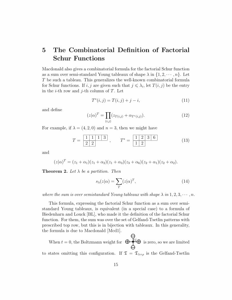
Macdonald also gives a combinatorial formula for the factorial Schur functionas a sum over semi-standard Young tableaux of shape λ in {1, 2, · · · , n}. LetT be such a tableau. This generalizes the well-known combinatorial formulafor Schur functions. If i, j are given such that j 6 λi, let T (i, j) be the entryin the i-th row and j-th column of T . Let

T ∗(i, j) = T (i, j) + j − i, (11)

and define(z|α)T =

∏(i,j)

(zT (i,j) + αT ∗(i,j)). (12)

For example, if λ = (4, 2, 0) and n = 3, then we might have

T =1 1 1 3

2 2, T ∗ =

1 2 3 6

1 2(13)

and

(z|α)T = (z1 + α1)(z1 + α2)(z1 + α3)(z3 + α6)(z2 + α1)(z2 + α2).

Theorem 2. Let λ be a partition. Then

sλ(z|α) =∑T

(z|α)T , (14)

where the sum is over semistandard Young tableaux with shape λ in 1, 2, 3, · · · , n.

This formula, expressing the factorial Schur function as a sum over semi-standard Young tableaux, is equivalent (in a special case) to a formula ofBiedenharn and Louck [BL], who made it the definition of the factorial Schurfunction. For them, the sum was over the set of Gelfand-Tsetlin patterns withprescribed top row, but this is in bijection with tableaux. In this generality,the formula is due to Macdonald [Mcd1].

When t = 0, the Boltzmann weight forij

is zero, so we are limited

to states omitting this configuration. If T = Tλ+ρ is the Gelfand-Tsetlin

15

pattern corresponding to this state, and if the entries of T in are denotedpik as in (5), it is easy to see that the equality pi−1,k−1 = pi,k would causethis configuration to appear at the i, j position, where j = pi,k. Thereforepi−1,k−1 > pi,k. This inequality implies that we may obtain another Gelfand-Tsetlin pattern Tλ with top row λ by subtracting ρn−i+1 = (n − i + 1, n −i, · · · , 1) from the i-th row of Tλ+ρ.

Consider the example of λ = (4, 2, 0) with n = 3. Then

if Tλ+ρ =

7 4 1

5 34

then Tλ =

4 2 0

3 23

.We associate with Tλ a tableau T (Tλ) of shape λ. In this tableau, removingall boxes labeled n from the diagram produces a tableau whose shape is the

second row of Tλ. Then removing boxes labeled n− 1 produces a tableauwhose shape is the third row of Tλ, and so forth. Thus in the example, T (Tλ)is the tableau T in (13). Let w0 denote the long element of the Weyl groupSn, which is the permutation i 7→ n+ 1− i.

Proposition 4. Let t = 0, and let s = s(Tλ+ρ) be the state corresponding toa special Gelfand-Tsetlin pattern Tλ+ρ. With Tλ as above and T = T (Tλ) wehave

w0

(∏v∈s

βs(v)

)= zw0(δ)(z|a)T . (15)

Before describing the proof, let us give an example. With Tλ+ρ as above,the state s(Tλ+ρ) is

+

+

+

− + + − + + −

+ + − + − + +

+ + + − + + +

+ + + + + + +

−

−

−

− − + − + +

+ + − + − −

+ + + − − −

11121314151617

21222324252627

31323334353637

16

The locations labeled ◦ produce powers of zi, and the locations labeled •produce shifts of the form zi + αj. The weight of this state is∏

v∈s

βs(v) = z21z2(z1 + α6)(z2 + α2)(z2 + α1)(z3 + α3)(z3 + α2)(z3 + α1).

Applying w0 interchanges zi ←→ z4−i. The factor z21z2 becomes z2

3z2 = zw0(δ),and the terms that remain agree with∏

(i,j)

(zT (i,j) + αT ∗(i,j)).

Proof. We are using the following Boltzmann weights.

GammaIce

ij ij ij ij ij ij

Boltzmannweight

1 zi 0 zi + αj zi 1

We have contributions of zi from vertices that have − on the vertical edgebelow, and there is one of these for each entry in the Gelfand-Tsetlin pattern.These contribute a factor of zδ. Applying w0 to z leads to zw0(δ).

Considering the contribution from the (i, j) vertex, there will be a factor

of zi + αj when the vertex has the configurationij

. In the above

example, the locations are labeled by •.Let Tλ+ρ be the Gelfand-Tsetlin pattern (5). Let Tλ and T = T (Tλ) be as

described above, and let T ∗ be as in (11). Let the entries in Tλ+ρ and Tλ bedenoted pi,j and qi,j, with the indexing as in (5). Thus qi,j = pi,j −n+ j− 1.We will make the convention that qi,n+1 = pi,n+1 = 0. The condition for •in the i, j position of the state is that for some k with i 6 k 6 n we havepi+1,k+1 < j < pi,k. Translating this in terms of the qi,j = pi,j − n+ j − 1 thecondition becomes qi+1,k+1 + n − k + 1 6 j < qi,k + n − k. The effect of w0

is to interchange zi ↔ zn−i+1, and therefore

w0

(∏v∈s

βs(v)

)= zw0(δ)

n∏i=1

n∏k=i

qi,k+n−k∏j=qi+1,k+1+n−k+1

(zn+1−i + αj). (16)

17

On the other hand, in the tableau T , the location of the entries equal ton+ 1− i in the (k+ 1− i)-th row is between columns qi+1,k+1 + 1 throughqi,k, and if j is one of these columns then

T (k + 1− i, j) = n+ 1− i, T ∗(k + 1− i, j) = n+ j − k.

Therefore in the notation (12) we have

(z|α)T =n∏i=1

n∏k=i

qi,k∏j=qi+1,k+1+1

(zn+1−i + αn+j−k).

This equals (16) and the proof is complete.

We now give the proof of Theorem 2. Summing over states, the lastProposition implies that

Zλ(w0(z), α, 0) = zw0(δ)∑T

(z|a)T .

Since sΓλ(z, α, 0) = sΓ

λ(w0(z), α, 0) we have

sΓλ(z, α, 0) =

Zλ(w0(z), α, 0)∏i>j w0(z)j

=zw0(δ)

∑T (z|a)T

zw0(δ)=∑T

(z|a)T ,

and the statement follows.

6 The limit as t tends to infinity

Let µ be a partition, and let αµ denote the sequence

αµ = (αµ1+n, αµ2+n−1, · · · , αµn+1).

If λ is a partition then λ′ will denote the conjugate partition whose Youngdiagram is the transpose of that of λ.

Theorem 3. (Vanishing Theorem) We have

sλ(−αµ|α) =

{0 if λ 6⊂ µ,∏

(i,j)∈λ(αn−i+λi+1 − αn−λ′j+j) if λ = µ.

18

See Okounkov [Ok] Section 2.4 and Molev and Sagan [MS]. In view ofthe relationship between Schubert polynomials for Grassmannian permuta-tions and factorial Schur functions, this is equivalent to an older vanishingstatement for Schubert polynomials. Vanishing properties for Schubert poly-nomials are implied by Theorem 9.6.1 and Proposition 9.6.2 of Lascoux [La1],which are related to the results of Lascoux and Schutzenberger [LS2, LS3].We will prove it in this section by our methods.

We examine the behavior of our six-vertex model as we send the pa-rameter t to infinity. The first result of this section may be construed asa rederivation of a theorem of Lascoux [La2, Theorem 1]. However the ap-proach we take is to interpret it as giving us a proof of the equivalence offactorial Schur functions and double Schubert polynomials for Grassman-nian permutations. We also obtain the vanishing theorem for factorial Schurfunctions (Theorem 3).

We start with two simple lemmas. To state these, we describe the sixadmissible arrangements of edge spins around a vertex as types a1, a2, b1, b2,c1 and c2 respectively, when reading from left to right in the diagram (2).

Lemma 2. In each state, the total number of sites of type a2, b1 and c1 isequal to n(n− 1)/2.

Proof. This number is equal to the number of minus spins located in theinterior of a vertical string.

Let µ be the partition (λ+ δ)′.

Lemma 3. In each state, the number of occurrences of a2, b2 and c1 patternsin the i-th column is equal to µi.

Proof. This number is equal to the number of minus spins located on ahorizontal string between the strings labeled i and i + 1. This count isknown since for any rectangle, knowing the boundary conditions on the top,bottom and rightmost sides determines the number of such spins along theleftmost edge.

As a consequence of Lemma 2, the result of taking the limit as t→∞ canbe interpreted as taking the leading degree term in t for each of the Boltzmannweights vΓ(i, j, t) as in Section 4. Thus with the set of Boltzmann weights(1,−αj, 1, zi + αj, zi, 1) and corresponding partition function Z(SΓ

λ,∞), wehave

Z(SΓλ,∞) = zδsλ(z|α).

19

By Lemma 3, if we consider our ice model with the series of Boltzmannweights in the following diagram, then the corresponding partition functionis given by dividing Z(SΓ

λ,∞) by (−α)µ.

GammaIce

ij ij ij ij ij ij

Boltzmannweight

1 1 1 −zi/αj − 1 −zi/αj 1

Let us denote the partition function for this set of Boltzmann weights byZ(SΓ′

λ,∞(z|α)). Thus we obtain the result of [McN, Theorem 1.1],

Z(SΓ′

λ,∞(z|α)) =zδ

(−α)(λ+δ)′sλ(z|α). (17)

We now pause to introduce the notions of double Schubert polynomialsand Grassmannian permutations so that we can make the connection to [La2,Theorem 1] precise.

A permutation is Grassmannian if it has a unique (right) descent.Let n and m be given and let λ = (λ1, · · · , λn) be a partition such that

λ1 6 m. Then there is associated with λ a Grassmannian permutationwλ ∈ Sn+m. This is the permutation such that

wλ(i) =

{λn+1−i + i if i 6 n,i− λ′i−n if i > n,

where λ′ is the conjugate partition. This has wλ(n+1) < wλ(n) and no otherdescent.

Let x1, · · · , xn+m and y1, · · · , yn+m be parameters. We define the divideddifference operators as follows. If 1 6 i < n + m and f is a function of thexi let

∂if(x1, · · · , xn+m) =f − sifxi − xi+1

where sif is the function obtained by interchanging xi and xi+1. Then ifw ∈ Sn+m, let w = si1 · · · sik be a reduced expression of w as a product ofsimple reflections. Then let ∂w = ∂i1 · · · ∂ik . This is well-defined since thedivided difference operators ∂i satisfy the braid relations. Let w0 be the long

20

element of Sn+m. Then the double Schubert polynomials, which were definedby Lascoux and Schutzenberger [LS1] are given by

Sw(x, y) = ∂w−1w0

( ∏i+j6n+m

(xi − yj)

).

The theory of factorial Schur functions is a special case of the theoryof double Schubert polynomials developed by Lascoux and Schutzenberger[LS1, LS2]. Although the comparison is well-known, there does not appearto be a truly satisfactory reference in the literature. We give a new proof inthe thematic spirit of this paper.

Theorem 4. The factorial Schur functions are equal to double Schubert poly-nomials for Grassmannian permutations. More precisely,

Swλ(x, y) = sλ(x| − y)

Proof. The proof is a comparison of (17) with [La2, Theorem 1]. To translatethe left-hand side in (17) into the staircase language of Lascoux we use thebijection in Proposition 2. In Theorem 1 of [La2] if Lascoux’ x is our zand his y is our −α, then the left-hand side of his identity is exactly thepartition function on the left-hand side of our (17). The monomial xρry−〈u〉

on the right-hand side of his identity equals the monomial zρ(−α)−(λ+δ)′ onthe right-hand side of (17). Lascoux’ Xu,uω is the double Schubert polynomialSwλ . The statement follows.

To conclude this section, we shall use this description to give a proofof the characteristic vanishing property of Schur functions. In lieu of (17)above, the following result is clearly equivalent to Theorem 3.

Theorem 5. For two partitions λ and µ of at most n parts, we have

Z(SΓ′

λ,∞(−αµ|α)) = 0 unless λ ⊂ µ,

Z(SΓ′

λ,∞(−αλ|α)) =∏

(i,j)∈λ

(αn+1−i+λiαn−λ′j+j

− 1

).

Proof. Fix a state, and assume that this state gives a non-zero contribution tothe partition function Z(SΓ′

λ,∞(−αµ|α)). Under the bijection between states

21

of square ice and strict Gelfand-Tsetlin patterns, let ki be the leftmost entryin the i-th row of the corresponding Gelfand-Tsetlin pattern. We shall proveby descending induction on i the inequality

n+ 1− i+ µi ≥ ki.

For any j such that ki+1 < j < ki, there is a factor (xi/αj − 1) in theBoltzmann weight of this state. We have the inequality n+ 1− i+ µi > n+1−(i+1)+µi+1 ≥ ki+1 by our inductive hypothesis. Since (αµ)i = αn+1−i+µi ,in order for this state to give a non-zero contribution to Z(SΓ′

λ,∞(−αµ|α)),we must have that n+ 1− i+ µi ≥ ki, as required.

Note that for all i, we have ki ≥ n + 1 − i + λi. Hence µi ≥ λi for all i,showing that µ ⊃ λ as required, proving the first part of the theorem.

To compute Z(SΓ′

λ,∞(−αλ|α)), notice that the above argument shows thatthere is only one state which gives a non-zero contribution to the sum. Underthe bijection with Gelfand-Tsetlin patterns, this is the state with pi,j = p1,j

for all i, j. The formula for Z(SΓ′

λ,∞(−αλ|α)) is now immediate.

7 Asymptotic Symmetry

Macdonald [Mcd1] shows that the factorial Schur functions are asymptoticallysymmetric in the αi as the number of parameters zi increases. To formulatethis property, let σ be a permutation of the parameters α = (α1, α2, · · · ) suchthat σ(αj) = αj for all but finitely many j. Then we will show that if thenumber of parameters zi is sufficiently large, then sλ(z|σα) = sλ(z|α). Howlarge n must be depend on both λ and on the permutation σ.

We will give a proof of this symmetry property of factorial Schur functionsusing the Yang-Baxter equation. In the following theorem we will use the

22

following Boltzmann weights:

v1 zi − tα t zi + α zi(t+ 1) 1

w1 zi − tβ t zi + β zi(t+ 1) 1

u1 1 α− β 0 1 1

Theorem 6. With the above Boltzmann weights, and with ε1, · · · , ε6 fixedspins ±, the following two systems have the same partition function.

δ

ψφ

ε2ε1

ε3ε6

ε4ε5

w v

u

ε2ε1

νµ

ε3γε6

ε4ε5

u

v w

Proof. This may be deduced from Theorem 3 of [BBF] with a little work. Byrotating the diagram 90◦ and changing the signs of the horizontal edge spins,this becomes a case of that result. The R-matrix is not the matrix for ugiven above, but a constant multiple. We leave the details to the reader.

Let σi be the map on sequences α = (α1, α2, · · · ) that interchanges αiand αi+1. Let λ be a partition. We will show that sometimes:

sλ(z|α) = sλ(z|σiα) (18)

and sometimes

sλ(z|α) = sλ(z|σiα) + sµ(z|σiα)(αi − αi+1), (19)

23

where µ is another partition. The next Proposition gives a precise statementdistinguishing between the two cases (18) and (19).

Proposition 5. (i) Suppose that i + 1 ∈ λ + ρ but that i /∈ λ + ρ. Let µ bethe partition characterized by the condition that µ+ ρ is obtained from λ+ ρby replacing the unique entry equal to i + 1 by i. Then (19) holds with thisµ.

(ii) If either i+ 1 /∈ λ+ ρ or i ∈ λ+ ρ then (18) holds.

For example, suppose that λ = (3, 1) and n = 5. Then λ+ ρ = (8, 5, 3, 2, 1).If i = 4, then i + 1 = 5 ∈ λ + ρ but i /∈ λ + ρ, so (19) holds with µ + ρ =(8, 4, 3, 2, 1), and so µ = (3).

Proof. We will use Theorem 6 with α = αi and β = αi+1. The parameter tmay be arbitrary for the following argument. We first take i = n and attachthe vertex u below the i and i + 1 columns, arriving at a configuration likethis one in the case n = 3, λ = (4, 3, 1).

u

+

+

+

+ − + − + + − +

+ + +

+ +

+ + +

−

−

−

1112131415161718

2122232425262728

3132333435363738

There is only one legal configuration for the spins of the edges between u andthe two edges above it, which in the example connect with (3, 5) and (3, 4):these must both be +. The Boltzmann weight at u in this configurationis unchanged, and the partition function of this system equals that of SΓ

λ,t.After applying the Yang-Baxter equation, we arrive at a configuration with

24

the u vertex above the top row, as follows:

u

+

+

+

+ − +

− +

+ − +

+ + + + + + + +

−

−

−

1112131415161718

2122232425262728

3132333435363738

Now if we are in case (i), the spins of the two edges are −, + then there aretwo legal configurations for the vertex, and separating the contribution thesewe obtain

Z(Sλ,t) = (σiZ(Sλ,t)) + (α− β) (σiZ(Sµ,t)) .

If we are in case (ii), there is only one legal configuration, so Z(Sλ,t) =(σiZ(Sλ,t)) .

Corollary 1. Let λ be a partition, and let l be the length of λ. If n > l + ithen sλ(z|a) = sλ(z|σia).

Proof. For if l is the length of the partition λ, then the top edge spin incolumn j is − when j 6 n− l, and therefore we are in case (i).

This Corollary implies Macdonald’s observation that the factorial Schurfunctions are asymptotically symmetric in the αi.

8 The Dual Cauchy Identity

Let m and n be positive integers. For a partition λ = (λ1, . . . , λn) withλ1 ≤ m, we define a new partition λ = (λ1, . . . , λm) by

λi = |{j | λj ≤ m− i}|.

25

After a reflection, it is possible to fit the Young diagrams of λ and λ into arectangle.

We shall prove the following identity, known as the dual Cauchy identity.Another proof may be found in Macdonald [Mcd1] (6.17). In view of therelationship between factorial Schur functions and Schubert polynomials, thisis equivalent to a statement on page 161 of Lascoux [La1]. See also Corollary2.4.8 of Manivel [Ma] for another version of the Cauchy identity for Schubertpolynomials.

Theorem 7 (Dual Cauchy Identity). For two finite alphabets of variablesx = (x1, . . . , xn) and y = (y1, . . . , ym), we have

n∏i=1

m∏j=1

(xi + yj) =∑λ

sλ(x|α)sλ(y| − α).

The sum is over all partitions λ with at most n parts and with λ1 ≤ m.

Proof. The proof will consist of computing the partition function of a partic-ular six-vertex model in two different ways. We will use the weights vΓ(i, j, t)introduced in Section 4 with t = 1 and for our parameters (z1, . . . , zm+n), wewill take the sequence (ym, . . . , y1, x1, . . . , xn).

As for the size of the six-vertex model we shall use and the boundaryconditions, we take a (m+ n)× (m+ n) square array, with positive spins onthe left and lower edges, and negative spins on the upper and right edges.By Theorem 1 (with λ = 0), the partition function of this array is∏

i<j

(yi + yj)∏i,j

(yi + xj)∏i<j

(xi + xj).

We shall partition the set of all states according to the set of spins thatoccur between the rows with parameters y1 and x1. Such an arrangement ofspins corresponds to a partition λ in the usual way, i.e. the negative spinsare in the columns labeled λi + n − i + 1. In this manner we can write ourpartition function as a sum ∑

λ

Ztopλ Zbottom

λ .

Here Ztopλ is the partition function of the system with m rows, m + n

columns, parameters ym, . . . , y1 and boundary conditions of positive spins on

26

the left, negative spins on the top and right, and the λ boundary conditionspins on the bottom. And Zbottom

λ is the partition function of the systemwith n rows, m + n columns, spectral parameters x1, . . . , xn and the usualboundary conditions for the partition λ.

By Theorem 1, we have

Zbottomλ =

∏i<j

(xi + xj)sλ(x|α).

It remains to identify Ztopλ . To do this, we perform the following operation

to the top part of our system. We flip all spins that lie on a vertical strand,and then reflect the system about a horizontal axis. As a consequence, wehave changed the six-vertex system that produces the partition function Ztop

λ

into a system with more familiar boundary conditions, namely with positivespins along the left and bottom, negative spins along the right hand side,and along the top row we have negative spins in columns λi +m− i+ 1. TheBoltzmann weights for this transformed system are (since t = 1)

GammaIce

ij ij ij ij ij ij

Boltzmannweight

1 yi + αj 1 yi − αj 2yi 1

Now again we use Theorem 1 to conclude that

Ztopλ =

∏i<j

(yi + yj)sλ(y| − α).

Comparing the two expressions for the partition function completes the proof.

Bump: Department of Mathematics, Stanford University, Stanford, CA 94305-2125 USA.Email: bump@math.stanford.edu

McNamara: School of Mathematics and Statistics, University of Sydney, NSW, Australia.Email: mcnamara@maths.usyd.edu.au

Nakasuji: Department of Information and Communication Sciences, Faculty of Science and

Technology, Sophia University, 7-1 Kioi-cho, Chiyoda-ku, Tokyo 102-8554, Japan. Email:

nakasuji@sophia.ac.jp

27

References

[BR] A. Berele and A. Regev. Hook Young diagrams with applications tocombinatorics and to representations of Lie superalgebras. Adv. inMath., 64(2):118–175, 1987.

[BL] L. C. Biedenharn and J. D. Louck. A new class of symmetric polyno-mials defined in terms of tableaux. Adv. in Appl. Math., 10(4):396–438, 1989.

[BBF] B. Brubaker, D. Bump, and S. Friedberg. Schur polynomials and theYang-Baxter equation. Comm. Math. Phys., to appear.

[BG] D. Bump and A. Gamburd. On the averages of characteristic poly-nomials from classical groups. Comm. Math. Phys., 265(1):227–274,2006.

[CL] William Y. C. Chen and J. Louck. The factorial Schur function. J.Math. Phys., 34(9):4144–4160, 1993.

[GG] I. Goulden and C. Greene. A new tableau representation for super-symmetric Schur functions. J. Algebra, 170(2):687–703, 1994.

[GH] I. P. Goulden and A. M. Hamel. Shift operators and factorial sym-metric functions. J. Combin. Theory Ser. A, 69(1):51–60, 1995.

[HK] A. M. Hamel and R. C. King. Bijective proofs of shifted tableau andalternating sign matrix identities. J. Algebraic Combin., 25(4):417–458, 2007.

[IN] T. Ikeda and H. Naruse. Excited Young diagrams and equivariantSchubert calculus. Trans. Amer. Math. Soc., 361(10):5193–5221, 2009.

[KBI] V. Korepin, N. Boguliubov and A. Izergin Quantum Inverse Scatter-ing Method and Correlation Functions, Cambridge University Press,1993.

[KT] A. Knutson and T. Tao. Puzzles and (equivariant) cohomology ofGrassmannians. Duke Math. J., 119(2):221–260, 2003.

[Kr] V. Kreiman. Products of factorial Schur functions. Electron. J. Com-bin., 15(1):Research Paper 84, 12, 2008.

28

[La1] A. Lascoux,Symmetric functions and combinatorial operators on poly-nomials, CBMS Regional Conference Series in Mathematics, 99(2003).

[La2] A. Lascoux. The 6 vertex model and Schubert polynomials. SIGMASymmetry Integrability Geom. Methods Appl., 3:Paper 029, 12, 2007.

[LS1] A. Lascoux and M.-P. Schutzenberger. Polynomes de Schubert. C.R. Acad. Sci. Paris Ser. I Math., 294(13):447–450, 1982.

[LS2] A. Lascoux and M.-P. Schutzenberger. Interpolation de Newton aplusieurs variables, in Seminaire d’Algbre Paul Dubreil et Marie-PauleMalliavin Proceedings, Paris 1983–1984 (36eme Annee), Springer Lec-ture Notes in Mathematics 1146 (1985).

[LS3] A. Lascoux and M.-P. Schutzenberger. Decompositions dans l’algebredes differences divisees, Discrete Math., 99: 165–179 (1992).

[Lou] J. Louck. Unitary group theory and the discovery of the factorialSchur functions. Ann. Comb., 4(3-4):413–432, 2000. Conference onCombinatorics and Physics (Los Alamos, NM, 1998).

[Mcd1] I. G. Macdonald. Schur functions: theme and variations. InSeminaire Lotharingien de Combinatoire (Saint-Nabor, 1992), volume498 of Publ. Inst. Rech. Math. Av., pages 5–39. Univ. Louis Pasteur,Strasbourg, 1992.

[Mcd2] I. G. Macdonald. Symmetric functions and Hall polynomials. OxfordMathematical Monographs. The Clarendon Press Oxford UniversityPress, New York, second edition, 1995. With contributions by A.Zelevinsky, Oxford Science Publications.

[McN] P. J. McNamara. Factorial Schur functions via the six-vertex model.http://arxiv.org/abs/0910.5288, 2009.

[Mi] L. Mihalcea. Giambelli formulae for the equivariant quantum coho-mology of the Grassmannian. Trans. Amer. Math. Soc., 360(5):2285–2301, 2008.

29

[Ma] L. Manivel,Symmetric Functions, Schubert polynomials and degener-acy loci. SMF/AMS Texts and Monographs 6, American Mathemat-ical Society, Providence, RI; Societe Mathematique de France, Paris,2001.

[MS] A. I. Molev and B. Sagan. A Littlewood-Richardson rule for factorialSchur functions. Trans. Amer. Math. Soc., 351(11):4429–4443, 1999.

[Ok] A. Okounkov. Quantum immanants and higher Capelli identities.Transform. Groups, 1(1-2):99–126, 1996.

[OO1] A. Okounkov and G. Olshanskii. Shifted Schur functions. II. Thebinomial formula for characters of classical groups and its applica-tions. In Kirillov’s seminar on representation theory, volume 181 ofAmer. Math. Soc. Transl. Ser. 2, pages 245–271. Amer. Math. Soc.,Providence, RI, 1998.

[OO2] A. Okounkov and G. Olshanskii. Shifted Schur functions. Algebra iAnaliz, 9(2):73–146, 1997.

[To] T. Tokuyama. A generating function of strict Gelfand patterns andsome formulas on characters of general linear groups. J. Math. Soc.Japan, 40(4):671–685, 1988.

[ZJ1] P. Zinn-Justin. Littlewood-Richardson coefficients and integrabletilings. Electron. J. Combin. 16, 2009.

[ZJ2] P. Zinn-Justin. Six-Vertex, Loop and Tiling models: In-tegrability and Combinatorics, Habilitation Thesis, 2009.http://arxiv.org/abs/0901.0665.

30