Factors affecting the ultrasonic

intermodulation crack detection technique

using bispectral analysis

Charles R. P. Courtney, Bruce W. Drinkwater ∗,

Simon A. Neild, Paul D. Wilcox

Department of Mechanical Engineering, University of Bristol, Queens Building,

University Walk, Bristol BS8 1TR, United Kingdom

Abstract

This paper concerns the development of ultrasonic intermodulation as a method of

robustly detecting cracks in engineering components. The bispectrum signal anal-

ysis processing technique is used to analyse the nonlinear response of a sample to

continuous excitation at two frequencies. The increased nonlinearity due to defects

such as fatigue cracks is detected. The technique is shown to be insensitive to the

support conditions and excitation positions. The importance of the shape of the

excited modes is demonstrated and suggests that global inspection can be achieved

only by exciting multiple modes. This multi mode approach is then applied to the

detection of cracking of a steel steering actuator bracket.

Key words: Inter-modulation, Non-linear, Fatigue Crack, Bispectrum

PACS: 43.35.Zc, 43.25.Dc, 43.60.Wy

Preprint submitted to NDT&E Int. 5 September 2007

1 Introduction

This paper is concerned with the development of ultrasonic intermodulation

as a global method of detecting and monitoring fatigue cracks in engineering

components. The ultrasonic intermodulation method makes use of the nonlin-

ear response of cracked materials to an applied strain, by exciting the sample

at a pair of frequencies and observing the resultant mixing of the signals. The

work in this paper has lead to an improved understanding of the factors affect-

ing the sensitivity of the ultrasonic intermodulation technique through a series

of experiments, and progress the technique toward an industrially realisable

measurement.

Fatigue cracks resulting from fluctuating stresses are a major cause of failure

in engineering components and as such have attracted investigation for over a

century (1). Where fatigue cannot be avoided by careful design it is necessary

to undertake nondestructive testing to allow early detection of cracking and

minimize the risk of failure.

The main industrial nondestructive testing (NDT) methods inspect compo-

nents either by scanning (eddy current, ultrasound) or by using a wide field

of view (visual inspection, magnetic particle and penetrant testing) (2), but

none is global in the sense used here. A global testing technique allows a com-

ponent to be tested for damage without imaging or attempting to locate the

damage, the aim is to allow rapid evaluation of the state of a component with

a single measurement for the whole test object. This should allow easy inter-

pretation of the measurement and assessment of the continued viability of the

∗ Corresponding Author.

Email address: B.Drinkwater@bristol.ac.uk (Bruce W. Drinkwater).

2

component without requiring a great deal of interpretation by the operator or

scanning of a measurement probe over the component. The effect of damage

on the natural frequencies of a sample has been investigated as a potential

global inspection technique, but this approach has been proved to be sensitive

to environmental factors (3).

The large changes in nonlinear ultrasonic parameters for small degrees of dam-

age (4; 5; 6) have stimulated interest in the use of nonlinearity for fatigue

crack detection: nonlinear elastic wave spectroscopy shows promise as a route

to a sensitive crack detection method. Generation of harmonics of ultrasonic

signals, due to the nonlinear behavior of cracks in otherwise linear materi-

als, was demonstrated and proposed as a crack detection technique in the

late 1970s (7; 8) and continues to attract some interest for crack detection

(9; 4; 10; 11; 12) and the measurement of bond strength in adhesive joints

(13). At sufficiently high excitation amplitudes, subharmonics (signals with

frequency content at fractions of the applied ultrasonic frequency) can be gen-

erated (14) and these are being investigated as a method of detecting closed

cracks (15; 16). Donskoy et al. (17) demonstrated the vibroacoustic modula-

tion technique, where a sample excited with an ultrasound signal is probed

with a second low-frequency vibrational signal. When nonlinearity is present

signals will appear in the response at the sum and difference of the excitation

frequencies (sidebands) and these signals can be used to measure the degree

of damage. Donskoyet al. suggested and tested two modulation methods on

cracked steel pipes: impact modulation and continuous wave modulation. In

each case the ultrasound signal was >100 kHz and the modulation frequency

of the order of 1 kHz. Similarly Van Den Abeele et al. demonstrated the

technique on engine connecting rods using continuous modulation of <20 kHz

3

and a high frequency signal of 120-134 kHz (4). Duffour et al. (18) performed

experiments using a continuous modulation at 1 kHz, as well as experiments

using impact excitation, as the low frequency excitation. The effects of varying

the high frequency excitation over a wide range (50-230 kHz) and applying

compressive forces to the crack were considered and a damage index, defined

by results over a range of frequencies, was proposed to ensure reliable sensi-

tivity to cracks.

Hillis et al. (19) used vibroacoustic modulation with two ultrasonic signals

of similar order frequency (280 kHz and 462 kHz) and the same amplitude

to detect cracks in steel samples. More recent work by the same group has

looked at application of this technique to aircraft parts (20). The data was

analysed using bispectral analysis rather than the more commonly used power-

spectral analysis. Bispectral analysis is a signal processing technique (22; 23)

that, due to its sensitivity to quadratic phase coupling, has attracted interest

in dealing with nonlinear systems. The bispectrum was applied to a number

of different non-engineering nonlinear systems before. Fackrell et al. (24; 25)

applied it to the analysis of vibration signals and proposed its application

in machine condition monitoring. Howard (26) used bispectral analysis (and

trispectral analysis) to measure the coupling between frequency components

in the vibration of a helicopter gearbox. More recently attempts have been

made to apply bispectral analysis to crack detection problems using statistical

pattern recognition applied to the bispectrum of concrete structures excited

by impacts (27) or turbine blades excited by a shaker (28).

This paper starts with a short section defining the bispectrum and describing

its main features before discussing the experimental setup used. The results

section which follows includes experimental results relating to the dependence

4

of the intermodulation signal on crack length, how the sensitivity of the tech-

nique depends on the frequencies and amplitudes of the applied signals, the

position of the transducers and the support conditions. A multiple mode pro-

cess for applying the technique is proposed and demonstrated on a steering

actuator bracket.

1.1 Bispectral Analysis

Consider a signal x(t) with Fourier transform X(f), where t is time and f

frequency. The power spectrum is given by:

P (f) = E[X(f)X∗(f)] (1)

where E[. . .] is the expectation value operator and ∗ the complex conjugate.

If the power spectrum is regarded as second order then the bispectrum is the

third order given by:

B(f1, f2, f1 + f2) = E[X(f1)X(f2)X∗(f1 + f2)]. (2)

Note that the third argument of B, (f1 +f2) is dependent on the first two and

so is often omitted when writing the bispectrum: B(f1, f2) = B(f1, f2, f1+f2).

For clarity all three terms are retained here.

The bispectrum is complex and, as can be seen from equation (2), is a function

of two frequencies. The behavior of the bispectrum for continuous excitation

can be understood in terms of four properties required for it to be non-zero

5

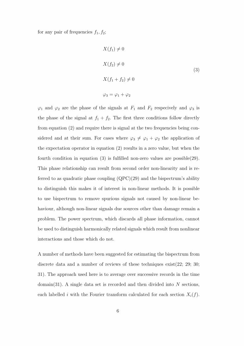
for any pair of frequencies f1, f2;

X(f1) 6= 0

X(f2) 6= 0

X(f1 + f2) 6= 0

ϕ3 = ϕ1 + ϕ2

(3)

ϕ1 and ϕ2 are the phase of the signals at F1 and F2 respecively and ϕ3 is

the phase of the signal at f1 + f2. The first three conditions follow directly

from equation (2) and require there is signal at the two frequencies being con-

sidered and at their sum. For cases where ϕ3 6= ϕ1 + ϕ2 the application of

the expectation operator in equation (2) results in a zero value, but when the

fourth condition in equation (3) is fulfilled non-zero values are possible(29).

This phase relationship can result from second order non-linearity and is re-

ferred to as quadratic phase coupling (QPC)(29) and the bispectrum’s ability

to distinguish this makes it of interest in non-linear methods. It is possible

to use bispectrum to remove spurious signals not caused by non-linear be-

haviour, although non-linear signals due sources other than damage remain a

problem. The power spectrum, which discards all phase information, cannot

be used to distinguish harmonically related signals which result from nonlinear

interactions and those which do not.

A number of methods have been suggested for estimating the bispectrum from

discrete data and a number of reviews of these techniques exist(22; 29; 30;

31). The approach used here is to average over successive records in the time

domain(31). A single data set is recorded and then divided into N sections,

each labelled i with the Fourier transform calculated for each section Xi(f).

6

The bispectrum estimate is then given as:

BX(f1, f2, f1+f2) =

∑Ni=1

Xi(f1)Xi(f2)X∗

i (f1 + f2)

N≈ E[X(f1)X(f2)X

∗(f1+f2)].

(4)

The time domain signals considered in this work are voltages across PZT disks

and the Fourier transforms are corrected for the window length to give the

frequency domain signals also in Volts. Using Fourier transform values in volts

in equation (4) gives bispectum values on Volts cubed (V3).

2 Experimental Procedure

Amplifier Scope/Signal Processor

SignalGenerator

SignalGenerator

Piezo-ceramic Disks

Crack

+

Fig. 1. Experimental Setup. Two signal generators produce sinusoidal electric sig-

nals. Signals are summed and amplified before passing to a piezoceramic disk bonded

to the sample. The resulting vibration produces a signal in a second disk, which is

passed to a PC for processing.

The ultrasonic intermodulation technique was applied to a series of samples

with varying degrees of damage by exciting them at two frequencies and mon-

itoring the content of the response at the difference or sum of the two applied

frequencies using bispectral analysis.

Experiments were undertaken using a set of four steel beams (60 mm × 60

mm × 400 mm). One sample was undamaged, the remaining three each had

7

a through crack at the mid-point of one side (shown schematically in Figure

1). These cracks were of 5 mm, 15 mm and 25 mm length respectively. The

samples were supported on two wires, positioned 50 mm from either end of

the sample, in an effort to minimize any nonlinearity at contacts between the

sample and its supports.

An excitation signal consisting of the sum of two sinusoidal signals was gener-

ated, amplified and then used to excite a 15-mm-diameter 2-mm-thick piezoce-

ramic disk bonded to the sample under investigation using a cynoacrylate ad-

hesive. The resulting vibration in the sample was detected by a 5-mm-diameter

2-mm-thick piezoceramic disk. The excitation frequencies were restricted to

the range 100 kHz-500 kHz by the response of the piezoceramic disks. To en-

sure good separation of the signals due to nonlinearity, the selected frequencies

were not integer multiples of each other. The continuous nature of the exci-

tation meant that, for appropriate frequencies, standing waves were set up in

the sample increasing the response. This was exploited by tuning each of the

excitation frequencies to a local maximum in the frequency response of the

system, corresponding to one of these vibrational modes. Having identified the

appropriate frequencies the applied voltage was adjusted to set the amplitude

received at each driving frequency to a predetermined level, to ensure compa-

rability of the mixing signals between tests. The response of the detector disk

to the vibration was sampled at 5 MHz digitized and passed to a PC. Each

data set consisted of 500000 data points which were divided into 488 sections

of 1024 points and the bispectrum estimated according to equation (4).

The process can be summarized as:

(1) Decide approximate excitation frequencies and desired amplitude in the

8

response.

(2) Apply first frequency to sample and tune to local maximum in sample

frequency response.

(3) Adjust driving voltage to give required response amplitude at that

frequency.

(4) Repeat steps 2 and 3 for second frequency.

(5) Apply both signals simultaneously to the sample.

(6) Record response for analysis offline.

3 Experimental Findings

The experiments undertaken can be broadly divided into two areas: those

looking at the fundamental behavior of the sample under excitation and those

investigating the effect of experimental factors. Starting with a demonstration

of the principle, the fundamental experimental results will be discussed first

followed by those relating to the particular experimental conditions, such as

transducer position and support conditions.

3.1 Investigation of Fundamental Behavior

3.1.1 Crack Detection with Ultrasonic Intermodulation and Bispectral Anal-

ysis

To demonstrate the ultrasonic intermodulation method (previously described

by Hillis et. al.(19)) each sample was excited at two vibrational modes (one

at 270±2 kHz and another at 473±2 kHz) and the exciting signal adjusted

so that the amplitude received at each driving frequency was 0.5 V. The

9

bispectrum of the response was evaluated and is shown in figure 2. In each

case there are six peaks in the bispectrum, which are the only points where

the bispectrum is non-zero. The two frequencies plotted are interchangeable

and so the bispectrum (as plotted) is symmetrical down the line f1 = f2. Due

to this symmetry the six peaks correspond to four features: the two harmonics

(the peaks B(F1, F1, 2F1) and B(F2, F2, 2F2), labelled ’1’ and ’2’ respectively

in figure 2) and the signals at the difference frequency (B(F1, F2 − F1, F2);

labelled ’3’) and the sum frequency (B(F1, F2, F1 + F2); labelled ’4’). Note

that the peak due to the harmonic of the higher frequency and the peak due

to the summed frequency signal rely on components of the signal that lie

outside the useful frequency range of the detection system (100kHz-500kHz)

Fig. 2. Variation of Bispectrum with Crack Length. Bispectrum plots for four steel

samples (60 mm × 60 mm × 400 mm), each excited at 270 kHz and 473 kHz to

produce 0.5 V amplitude in the received signal at those frequencies. a) undamaged

sample, and the remaining three had fatigue cracks introduced of b) 5 mm, c) 15

mm and d) 25 mm respectively. Peaks of interest are labelled 1-4.

10

and so are not a reliable measure of the nonlinear signal in this system.

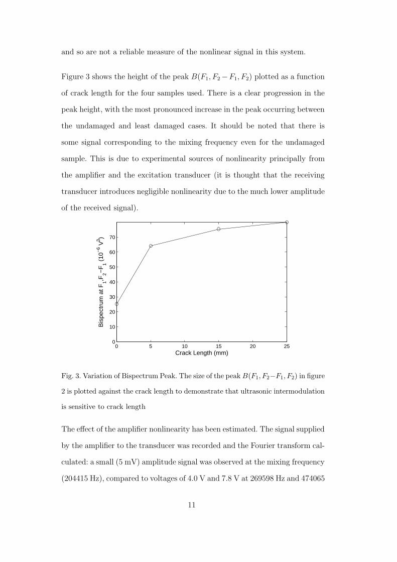
Figure 3 shows the height of the peak B(F1, F2 −F1, F2) plotted as a function

of crack length for the four samples used. There is a clear progression in the

peak height, with the most pronounced increase in the peak occurring between

the undamaged and least damaged cases. It should be noted that there is

some signal corresponding to the mixing frequency even for the undamaged

sample. This is due to experimental sources of nonlinearity principally from

the amplifier and the excitation transducer (it is thought that the receiving

transducer introduces negligible nonlinearity due to the much lower amplitude

of the received signal).

0 5 10 15 20 250

10

20

30

40

50

60

70

Crack Length (mm)

Bis

pect

rum

at F

1,F2−

F1 (

10−

6 V3 )

Fig. 3. Variation of Bispectrum Peak. The size of the peak B(F1, F2−F1, F2) in figure

2 is plotted against the crack length to demonstrate that ultrasonic intermodulation

is sensitive to crack length

The effect of the amplifier nonlinearity has been estimated. The signal supplied

by the amplifier to the transducer was recorded and the Fourier transform cal-

culated: a small (5 mV) amplitude signal was observed at the mixing frequency

(204415 Hz), compared to voltages of 4.0 V and 7.8 V at 269598 Hz and 474065

11

Hz (the driving frequencies). It was also found that a 50 V amplitude signal

at 204415 Hz applied to the system results in a 3.6 V amplitude response. If

it is assumed that the transducers and sample behave linearly, this indicates

that the 5 mV inputted due to the amplifier nonlinearity corresponds to 0.4

mV in the receiver signal. Using this and the measured voltages at 269598 Hz

and 474065 Hz (380 mV and 310 mV respectively) in equation 2 results in a

bispectrum peak of approximately 10 × 10−6 V3 due to the amplifier nonlin-

earity (a factor of eight was divided out due to the measurement of real signal

amplitudes, but the use of Fourier coefficients in equation 2). The bispectrum

peak measured for the undamaged case was 25 × 10−6V 3. This suggests that

the amplifier is one of the main causes of this nonlinearity. Separating the two

excitations, by using a separate amplifier and transducer for each applied fre-

quency, is a potential method of reducing the nonlinear effect of the amplifier

and transducer and ensuring that all mixing occurs in the sample, although

at the cost of some increase in experimental complexity and equipment. Tests

using two amplifiers and two transducers indicate a moderate (approximately

20%) reduction in the mixing signal for the undamaged sample (21). For sam-

ples requiring similar (or lower) levels of excitation to those considered in this

paper, the single amplifier and transducer configuration is both adequate and

experimentally simple. For particularly difficult-to-excite samples, or where

this configuration is not sufficiently sensitive, using separate amplifiers and

transducers may offer a solution. A test of the effect of the transducer-sample

contact on the nonlinearity is included in the next section.

12

3.1.2 Amplitude and Frequency Dependence

The signal used for the excitation of the system can be characterized by three

parameters: the two frequencies used and the amplitude of the response at each

of these frequencies (as only the case where applied voltage is adjusted to give

the same response voltage for both frequencies is considered here). In order

to investigate how these parameters affect the sensitivity of the technique to

damage the undamaged sample and the sample with the 25 mm crack were

used.

468 469 470 471 472 473 474 4750

5

10

15Undamaged

Out

put (

mV

)

Frequency (kHz)

468 469 470 471 472 473 474 4750

0.5

1

1.5

2

2.525mm Crack

Out

put (

mV

)

Frequency (kHz)

Fig. 4. Response of a) undamaged and b) 25-mm-cracked samples to a slowly swept

excitation signal. Excitation frequency was swept from 468 kHz to 475 kHz whilst

maintaining constant excitation voltage amplitude (20 V).

The implementation of ultrasonic intermodulation uses frequencies selected

to correspond to local maxima of the sample response. Figure 4 shows the

response of the samples excited by a slowly swept signal running from 468

kHz to 475 kHz at constant input amplitude over 100ms. The plot indicates

how high the modal density is and the number of possible choices of frequency

13

Table 1

Mean B(F1, F2 − F1, F2) values for 160 mV response at each frequency. Effect of

removing and replacing transducer.

B(F1, F2 − F1, F2) × 106V 3 at 160 mV

Mean St. Dev.

0.5 0.4

0.7 0.4

0.4 0.1

3.1 1.3

available, even over such a narrow range. The modal structure is different in

the two cases and so there is no guarantee that the same mode, with the

same mode shape, can be selected in each case. Behavior is similar in the

region around 270 kHz. Figure 5 shows the effect of applying the ultrasonic

intermodulation technique to a large number of modes in the region 468-

475 kHz and a fixed lower excitation frequency corresponding to the strongest

response in the region 269-271 kHz (270693 Hz for the undamaged sample and

269243 Hz for the cracked sample). The applied voltage at each of frequency

pair was changed for each measurement, such that the responses at F1 and

F2 remained equal to each other and increased from 10mV to 200mV over

20 measurements per pair. Although results for the damaged and undamaged

case clearly differ, each set of results varies widely with the upper frequency

used. This indicates that, if only a single pair of modes is used, for some

choices of modes the ability to detect a crack is reduced.

The mean value (averaged over all the modes shown) of each data set is plotted

14

alongside the individual mode results (indicated with dots). For comparison,

with a 160 mV response at the driving frequencies, the mean for the undam-

aged specimen was 0.7× 10−6 V3 with a standard deviation of 0.4× 10−6 V3

and for the 25-mm-cracked specimen 14.0×10−6 V3 with a standard deviation

of 4.5 × 10−6 V3. The nonlinearity of the amplifier was identified, in section

3.1.1, as a major source of experimental nonlinearity for undamaged samples.

The contact between the input transducer and the sample was another po-

tential source of nonlinearity and so the transducer used on the undamaged

sample was removed, replaced and the experiment repeated. This was done a

total of four times and the results are shown in table 1. As can be seen there is

some variation in the average value; the final result is somewhat higher than

the others, however it does not approach the value obtained for the damaged

sample.

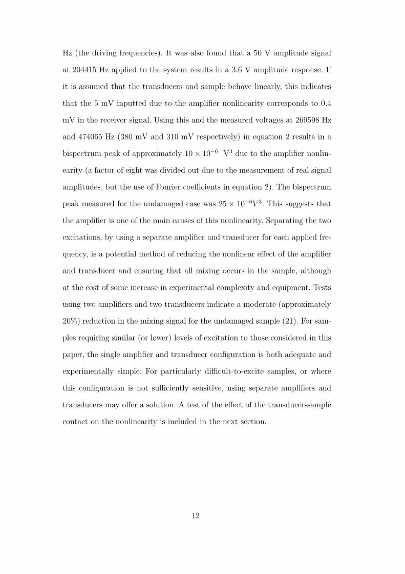
Figure 6 shows the increase in the bispectrum peak B(F1, F2 − F1, F2) with

increasing vibration at a given pair of driving frequencies on a log-log plot.

The damaged sample results follow the power law B(F1, F2−F1, F2) ∝ Xβ(Fi)

where X(Fi) = X(F1) = X(F2). Least-squares fitting to the data in figure 6

gives an average (over all the considered modes) gradient of β = 3.97 (standard

deviation, 0.11) for the cracked sample. β = 4 for a quadratic nonlinearity(19).

The undamaged sample undergoes a shift in gradient in figure 6 at approx-

imately 50 mV amplitude (-1.3 on the log scale) at each driving frequency:

below this value the average gradient, β = 2.27 (standard deviation, 0.26) and

above the gradient, β = 3.70 (standard deviation, 0.34). From equation 2 it

can be seen that a constant value of the amplitude at the difference signal

will lead to β = 2. A value of β = 2 would be expected if the only signal,

X(F2 −F1), were a noise unrelated to the excitation amplitude. The behavior

15

of the undamaged sample suggests that there is a small source of nonlinear-

ity that is initially smaller than a noise floor, but exceeds this level once the

linear response at the excitation frequencies exceeds 50 mV, whereas in the

damaged sample the amplitude-dependent nonlinear signal exceeds the static

noise value at all excitation amplitudes considered.

0 20 40 60 80 100 120 140 160 180 2000

10

20

30

40

50

60

Response amplitude at the F1 and F

2 driving frequencies (mV)

Bis

pect

rum

at F

1,F2−

F1 (

10−

6 V3 )

Undamaged: F1 = 270693Hz

25mm Crack:F1 = 269243Hz

Fig. 5. Effect of mode selection and vibration amplitude on ultrasonic intermodu-

lation signals. Local maxima in the frequency response of the samples in the region

468-475 kHz were identified and intermodulation measurements made for each. The

bispectrum peaks B(F1, F2 − F1, F2) are plotted as a function of amplitude for all

the modes selected for the undamaged (dashed line) and 25-mm-cracked (solid line)

samples. The average over each set of modes is shown as a solid line with dots.

So far the results have been performed for a particular lower frequency vi-

brational state. Repeating the experiments, using the same transducer, for

another three low frequencies (F1 = 269243 Hz, 269396 Hz and 270540 Hz)

produces some variation in the average value of B(F1, F2 − F1, F2) over the

same set of F2 each time at 160 mV amplitude. The average over the F2

frequency range for the undamaged sample varies from 0.4 to 8 ×10−6V 3 de-

16

−2 −1.8 −1.6 −1.4 −1.2 −1 −0.8 −0.6−10

−9

−8

−7

−6

−5

−4

log10

(Amplitude at driving frequency)

log 10

B(F

1,F2−

F1,F

2)

Undamaged: F1 = 270693Hz

25mm Crack:F1 = 269243Hz

Fig. 6. Effect of mode selection and vibration amplitude on ultrasonic intermod-

ulation signals. The same data shown in figure5 is plotted on a log-log scale to

demonstrate the power law relationship between signal amplitude at the driving

frequencies and the nonlinear signal

pending on the F1 value used. This reflects the selection of modes with poorer

transfer of motion between the input and output transducers than the original

selections, requiring higher applied voltages and so more nonlinear signal from

the amplifier and transducer.

3.1.3 Modal Response

In order to investigate the effect of the selected mode further, the intermodu-

lation experiment was performed with a response amplitude of 0.5 V at each

excitation frequency, with F1 fixed and F2 corresponding to each of the vibra-

tional modes in the region 468-475 kHz. Figure 7 shows the resulting bispec-

trum signal B(F1, F2 − F1, F2) against the frequency of the higher mode (the

lower frequency, F1, remains at 271960 Hz throughout). As in figure 5 there

is a wide spread of response with frequency for a given excitation amplitude

17

and there is no apparent correlation between the response and the frequency.

468 469 470 471 472 473 474 4750

50

100

150

200

250

300

Bis

pect

rum

Pea

k at

F1,F

2−F

1 (10

−6 V

3 )

Frequency (kHz)

Undamaged25mm Crack

Fig. 7. Variation of nonlinearity with mode selected. Samples excited at fixed lower

frequency (F1 = 271900 Hz) excitation and upper frequencies from F2 =468 kHz

to F2 =475 kHz and excitation adjusted to give 0.5 V amplitude in the response at

each driving frequency.

A third piezoceramic disk was added at the midpoint of one (long) side 5 mm

from the edge, such that it was positioned across the crack of the 25 mm sam-

ple and at an equivalent position of the undamaged sample. Figure 8 shows

the bispectrum response, B(F1, F2 −F1, F2), against the peak-to-peak voltage

across the piezoceramic disk at the crack. The response amplitude at the crack

at F1 (which was fixed) was 0.1 V for all the measurements. The response am-

plitude at F2 at the crack varied from 0.03 V to 0.3 V (depending on the F2

value used). This results in the peak-to-peak response variation from 0.26 to

0.8 V seen in figure 8. From figure 8 it is clear that the mixing signal generated

by the system for a given vibration detected at the end point, remote from

the crack, depends on the level of vibration at the crack with a response very

close to the undamaged behavior for the lowest signals at the crack, increasing

18

sharply as the level of vibration increases before flattening at approximately

250×10−6V 3. There is no clear relationship between the response at the crack

position transducer and the bispectrum peak for the undamaged sample, as

would be expected. This result demonstrates the importance of exciting the

crack sufficiently at both frequencies to get the required mixing and the large

difference in the excitation at a particular point that occurs for different vi-

brational modes that are very similar in frequency. This presents a difficulty

in using the ultrasonic intermodulation with continuous excitation as great

care must be taken to ensure that the same mode is selected for each mea-

surement when a comparison is to be made and for any given mode pair there

will always be regions that are not excited at one or other frequency result-

ing in blind spots for the technique. This suggests that to properly test an

object multiple modes should be used, either simultaneously using broadband

excitation or concurrently by making multiple measurements using pairs of

continuous signals at different frequencies. From the averages plotted in figure

5 it appears that taking a straightforward average over a range of modes for a

given response amplitude at each of the driven modes offers a straightforward

solution although both modes would need to be varied rather than just the one

as in section 3.1.2. The importance of mode shape and selection to detection

sensitivity has also been an area of interest in the use of guided waves for de-

fect detection(32). There the solution is often appropriate selection of a single

mode(33; 34), although multimode approaches have been applied(35; 36).

19

0 0.1 0.2 0.3 0.4 0.5 0.6 0.7 0.80

50

100

150

200

250

300

Bis

pect

rum

Pea

k at

F1,F

2-F1 (

10-6

V3 )

Peak-to-peak Response at Crack Position (V)

Undamaged25mm Crack

Fig. 8. Variation of mixing signal with vibration at crack. Result shown in 7 plot-

ted against peak-to-peak voltage across piezoceramic disk positioned at crack (or

equivalent position on undamaged sample) as shown schematically in inset.

3.2 Experimental Factors

In addition to the amplitude and frequency of the signal applied to the system

there are other experimental factors that need to be considered when using the

ultrasonic intermodulation technique. Experiments have been undertaken to

evaluate the importance of the positions of the transducers used for excitation

and reception and the support conditions of the sample.

3.2.1 Excitation Positions

The samples were excited, as previously, with two sinusoidal frequencies tuned

to vibrational modes and with the exciting signal adjusted so that the ampli-

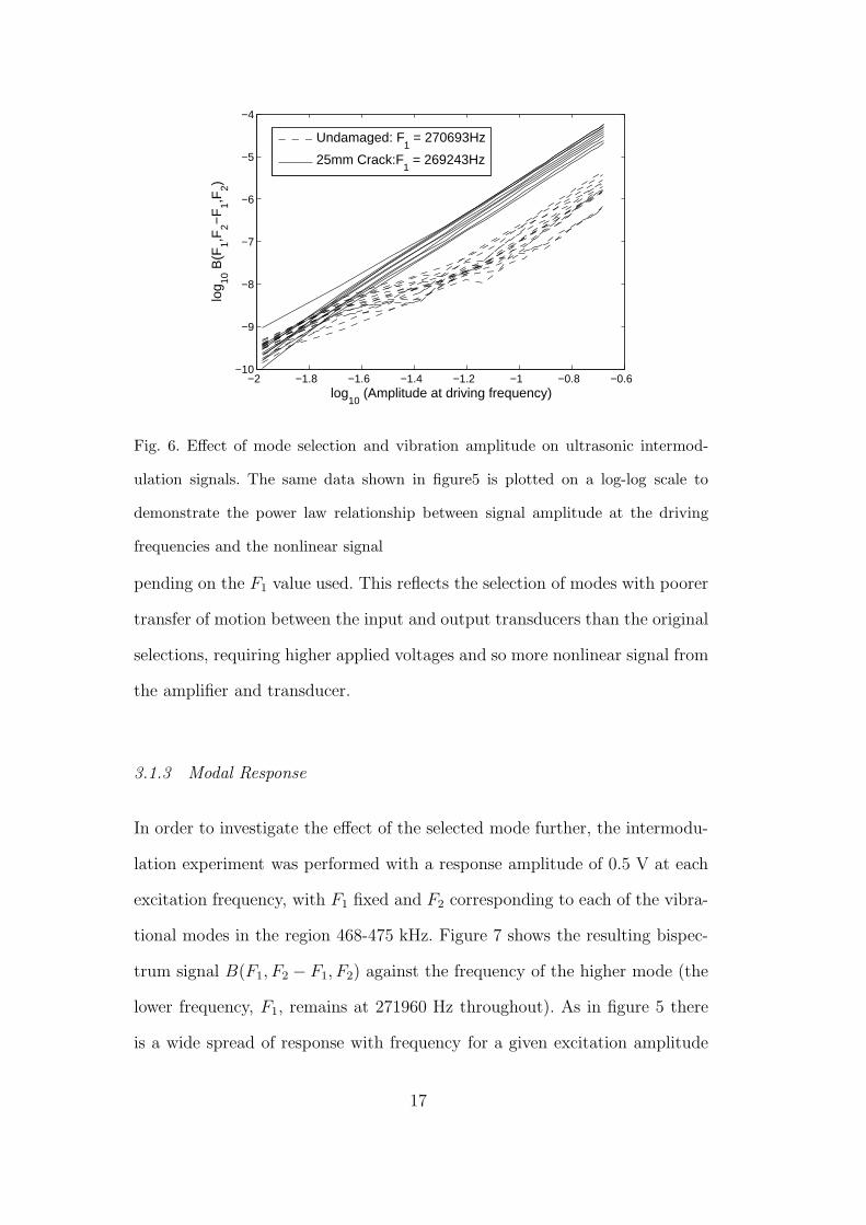
tude received at each driving frequency was 0.5 V. Figure 9 shows the resulting

bispectrum mixing peaks as a function of crack length for three transducer

20

configurations, via transducers located at the ends of the sample (as used pre-

viously), and two configurations with the transducers on the same side of the

sample as the crack: one with the transducers 40 mm from the ends (so that

the crack falls between them) and one with the driving transducer 40 mm

from one end and the receiving 80 mm from the same end. The configurations

are shown schematically, with the results in figure 9. Note that due to diffi-

culty reaching a sufficient level of excitation the configuration using two close

(40 mm separation) transducers was performed with F1 = 270 ± 2 kHz and

F2 = 440±2 kHz rather than F1 = 270±2 kHz and F2 = 473±2 kHz as with

the other two setups.

0 5 10 15 20 250

50

100

150

200

250

300

350

400

Crack Length (mm)

Bis

pect

rum

at F

1,F 2

-F1(

10-6V

3 )

(a)

(b)

(c)

(a)

(b)

(c)

Fig. 9. Effect of varying transducer position. Bispectrum peak, B(F1, F2 − F1, F2),

as a function of crack length for three different transducer configurations a) top

of sample 40 mm separation, b) top of sample 320 mm separation and c) opposite

ends.

Figure 9 shows that for each configuration there is a clear progression in

the signal due to the crack nonlinearity. The two configurations where the

transducers are either side of the crack are similar in behavior with a large

increase in signal between the undamaged and 5-mm-cracked states with a slow

increase as the crack grows. The configuration with two transducers closely

21

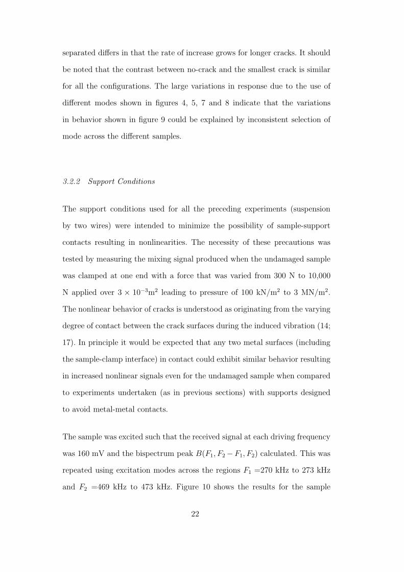
separated differs in that the rate of increase grows for longer cracks. It should

be noted that the contrast between no-crack and the smallest crack is similar

for all the configurations. The large variations in response due to the use of

different modes shown in figures 4, 5, 7 and 8 indicate that the variations

in behavior shown in figure 9 could be explained by inconsistent selection of

mode across the different samples.

3.2.2 Support Conditions

The support conditions used for all the preceding experiments (suspension

by two wires) were intended to minimize the possibility of sample-support

contacts resulting in nonlinearities. The necessity of these precautions was

tested by measuring the mixing signal produced when the undamaged sample

was clamped at one end with a force that was varied from 300 N to 10,000

N applied over 3 × 10−3m2 leading to pressure of 100 kN/m2 to 3 MN/m2.

The nonlinear behavior of cracks is understood as originating from the varying

degree of contact between the crack surfaces during the induced vibration (14;

17). In principle it would be expected that any two metal surfaces (including

the sample-clamp interface) in contact could exhibit similar behavior resulting

in increased nonlinear signals even for the undamaged sample when compared

to experiments undertaken (as in previous sections) with supports designed

to avoid metal-metal contacts.

The sample was excited such that the received signal at each driving frequency

was 160 mV and the bispectrum peak B(F1, F2 −F1, F2) calculated. This was

repeated using excitation modes across the regions F1 =270 kHz to 273 kHz

and F2 =469 kHz to 473 kHz. Figure 10 shows the results for the sample

22

469470

471472

473

270271

2722730

5

10

15

20

F2(kHz)

a)

469 470 471 472 473 474

270271

2722730

5

10

15

20

300N

b)

3000N

469470

471472

270271

2722730

5

10

15

20c)

10000N

469470

471472

473

270271

2722730

5

10

15

20

d)

BX

(F1,F

2-F

1) 1

0- 6V

3

473

F1(kHz) F2(kHz)F1(kHz)

F2(kHz)F1(kHz)F2(kHz)F1(kHz)

BX

(F1,F

2-F

1) 1

0- 6V

3B

X(F

1,F

2-F

1) 1

0- 6V

3

BX

(F1,F

2-F

1) 1

0- 6V

3

Fig. 10. Effect of Supoort Conduitions on Mixing Signal. The Bispectrum peak,

B(F1, F2−F1, F2), for all possible pairs of modes in the regions F1 =270 kHz to 273

kHz and F2 =469 kHz to 473 kHz excited to give 160 mV at each frequency in the

response. a) suspended the sample on wires as in all the previous experiments b),

c) and d) clamped the sample at one end with forces of 300N, 3000N and 10000N

respectively.

suspended on wires (as previously) and clamped at one end (as shown in the

figure) with a force of 300 N, 3000 N and 10,000 N over an area of 3×10−3m2.

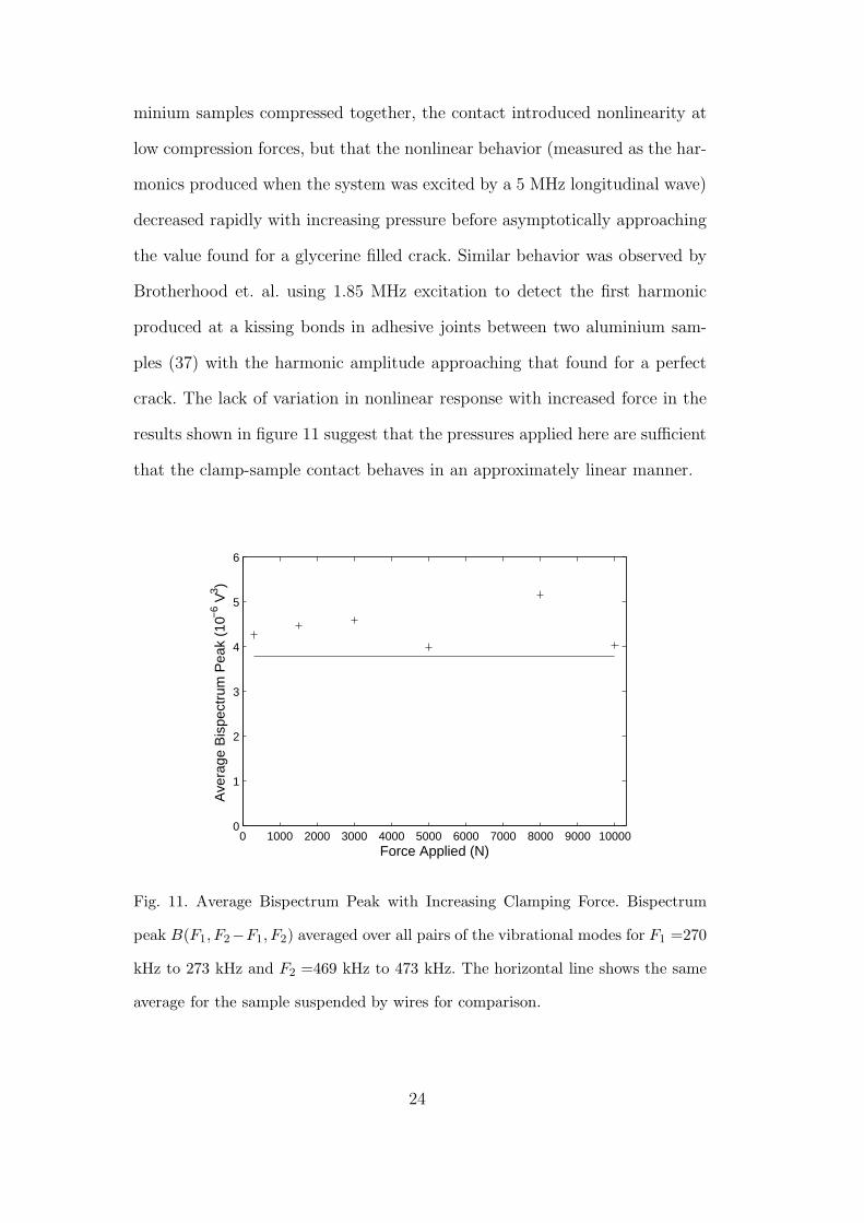
The behavior is similar for all the tested mode combinations. Figure 11 shows

the effect on the average peak value, over the frequency ranges considered, with

increasing force applied to the clamps. The average value for the suspended

sample is included for comparison. There is a small increase in the average

peak size when the sample is clamped rather than suspended, but this does not

appear to be clearly dependent on the force applied. The increase in the non-

linear signal between the suspended sample and the clamped samples is small

when compared to the increases found earlier between an undamaged sample

and a 25-mm-cracked sample. Buck et. al. (7) showed that for a pair of alu-

23

minium samples compressed together, the contact introduced nonlinearity at

low compression forces, but that the nonlinear behavior (measured as the har-

monics produced when the system was excited by a 5 MHz longitudinal wave)

decreased rapidly with increasing pressure before asymptotically approaching

the value found for a glycerine filled crack. Similar behavior was observed by

Brotherhood et. al. using 1.85 MHz excitation to detect the first harmonic

produced at a kissing bonds in adhesive joints between two aluminium sam-

ples (37) with the harmonic amplitude approaching that found for a perfect

crack. The lack of variation in nonlinear response with increased force in the

results shown in figure 11 suggest that the pressures applied here are sufficient

that the clamp-sample contact behaves in an approximately linear manner.

0 1000 2000 3000 4000 5000 6000 7000 8000 9000 100000

1

2

3

4

5

6

Force Applied (N)

Ave

rage

Bis

pect

rum

Pea

k (1

0−6 V

3 )

Fig. 11. Average Bispectrum Peak with Increasing Clamping Force. Bispectrum

peak B(F1, F2−F1, F2) averaged over all pairs of the vibrational modes for F1 =270

kHz to 273 kHz and F2 =469 kHz to 473 kHz. The horizontal line shows the same

average for the sample suspended by wires for comparison.

24

4 Multiple Mode Method

The method of performing measurements for combinations of modes from two

frequency regions, used in section 3.2.2, was applied to a real aeronautical

part (a steering actuator bracket) with an artificially grown fatigue crack to

demonstrate its use to detect damage in engineering components. First there

is a more precise outline of the proposed method, followed by a description of

the sample and the results associated.

4.1 Proposed Method

The approach proposed, in order to apply the inter-modulation technique

whilst removing the difficulties due to the sensitivity of the response to the

modes selected, is to identify all the modes in two frequency regions and

analyse the response of the sample as all combinations of one low and one

high frequency. The approach for each pair is the same as described in section

2. Modes are identified by measuring the response of the sample to a slowly

swept signal, with local maxima in the response giving the modal frequencies.

(1) Choose excitation frequency ranges and desired amplitude in the

response.

(2) Apply signal swept across first frequency range and record response.

(3) Perform Fourier transform and locate local maxima in response.

(4) Repeat steps 2 and 3 for second frequency range.

(5) Select one pair of modes and apply sinusoidal signals at those

frequencies.

(6) Adjust input to give desired response at each mode.

25

(7) Repeat steps 5 and 6 for each combination of modes.

(8) Evaluate mixing signal at each pair.

(9) Use statistical measure of peaks over all pairs to evaluate damage.

4.2 Steering Actuator Bracket

A pair of steering actuator brackets from a Let L410 commuter aircraft were

supplied to us by the Czech Aeronautical Research and Test Institute (VZLU)one

undamaged and one that has been artificially fatigued, resulting in a crack at

the critical point (marked on figure 12) perpendicular to the surface, with a

visible length of 9mm and depth of 3mm, constituting approximately 10-15%

of the cross-sectional area (the sample has a 12mm by 15mm cross-section at

the critical point). Figure 12 shows the shape of the steering actuator bracket

along with the positions of for piezoceramic disks (labelled A-D) bonded to it.

All the disks were 5-mm-diameter 2-mm-thick disks bonded with cyanoacry-

late adhesive.

A

C

B

D

Crack Position

260mm

160mm

Fig. 12. Steering Actuator Bracket from a Let L410 commuter aircraft with trans-

ducer positions labelled A-D. Sample provided by Aeronautical Research and Test

Institute (VZLU), Prague

26

Initially disk A was used for excitation of the sample and disk B to record

the response. The lower excitation frequencies (F1) were the local maxima in

the response of the sample to a swept signal from 270kHz to 272KHz, and

the higher excitation frequencies (F2) were in the region 472 kHz to 474 kHz.

There were 9 modes in the lower region and 7 in the upper, leading to a total of

63 pairs. At each of these pairs the excitation amplitudes were adjusted to give

a response of 100mV at each of the two excitation frequencies. The resulting

response at disk B was recorded and the bispectrum calculated. Figure 13

shows the peak B(F1, F2 − F1, F2) for both the damaged and undamaged

samples plotted both as a function of the exciting frequencies and also as a

distribution of peak values over each set of mode pairs. There is a broad spread

of results for both damaged and undamaged samples, but the damaged case

has more high values and a higher maximum. The undamaged bracket results

in a mean peak of 1.3 × 10−6 V3 with a standard deviation of 1.7 × 10−6 V3,

testing the damaged sample gives a mean of 3.7 × 10−6 V3 with a standard

deviation of 3.2× 10−6 V3. Table 2 shows the same process repeated for three

other transducer pairs and lists the mean, standard deviation and spread of

values for each set of results. In each case there is an overlap in the spreads

between the damaged and undamaged cases, reiterating that use of single

pairs of modes is likely to be unreliable, but in each case there is a clear

difference between the mean values and the standard deviations when the

bracket contains damage compared to the undamaged case. The choice of

the mean represents a viable and straightforward statistical measure of the

increased non-linearity, more elaborate measures may also present a method of

improving the method, in particular the use of the average removes any spatial

information that could be obtained from the mode shapes. Although it would

require a very good understanding of the modes of the sample, in principle it

27

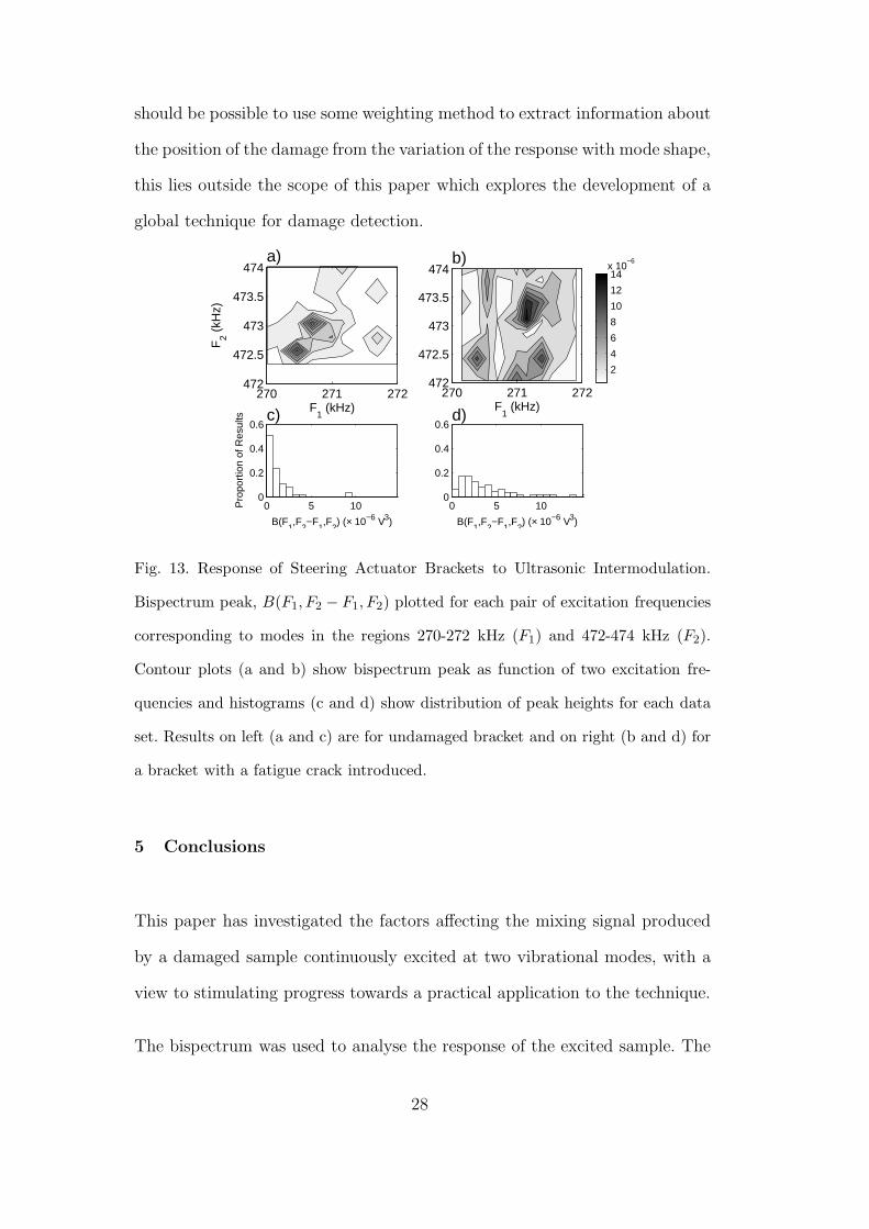
should be possible to use some weighting method to extract information about

the position of the damage from the variation of the response with mode shape,

this lies outside the scope of this paper which explores the development of a

global technique for damage detection.

F1 (kHz)

F2 (

kHz)

a)

270 271 272472

472.5

473

473.5

474

F1 (kHz)

b)

270 271 272472

472.5

473

473.5

474

2

4

6

8

10

12

14x 10

−6

0 5 100

0.2

0.4

0.6

Pro

port

ion

of R

esul

ts

B(F1,F

2−F

1,F

2) (× 10−6 V3)

c)

0 5 100

0.2

0.4

0.6

B(F1,F

2−F

1,F

2) (× 10−6 V3)

d)

Fig. 13. Response of Steering Actuator Brackets to Ultrasonic Intermodulation.

Bispectrum peak, B(F1, F2 − F1, F2) plotted for each pair of excitation frequencies

corresponding to modes in the regions 270-272 kHz (F1) and 472-474 kHz (F2).

Contour plots (a and b) show bispectrum peak as function of two excitation fre-

quencies and histograms (c and d) show distribution of peak heights for each data

set. Results on left (a and c) are for undamaged bracket and on right (b and d) for

a bracket with a fatigue crack introduced.

5 Conclusions

This paper has investigated the factors affecting the mixing signal produced

by a damaged sample continuously excited at two vibrational modes, with a

view to stimulating progress towards a practical application to the technique.

The bispectrum was used to analyse the response of the excited sample. The

28

Table 2

Statistical Measures of Response of Steering Actuator Bracket to Two Frequency

Excitation

Transducers Undamaged Response Damaged Response

(×10−6V 3) (×10−6V 3)

Excitation Response Mean Standard

Devia-

tion

Spread Mean Standard

Devia-

tion

Spread

A B 1.3 1.6 0.1-9.5 3.5 3.2 0.3-14.7

A D 2.9 2.8 0.2-10.6 5.2 4.7 0.4-27.1

B C 0.9 0.9 0.1-4.5 3.7 3.6 0.4-16.7

C D 2.1 1.8 0.1-9.4 3.4 2.5 0.2-9.8

signal at the difference of the exciting frequencies was monitored and was

shown to be increased by the presence of damage. The technique was found

to be robust with regards the transducer position and the boundary condi-

tions and valid over a range of vibrational amplitudes (for a given frequency

pair). The key finding regarding the application of the technique was found

to be the level of vibration at the crack, which depends on the shape of the

modes selected. For experiments relying on a single pair of modes this makes

the method unduly fragile. A method that excites a number of modes, either

during one test or a series of consecutive tests, would remove the possibility

that a particular mode had been selected with a node positioned at the dam-

age. Such a method has been proposed and demonstrated on a geometrically

complex engineering part.

29

6 Acknowledgements

This work was funded as part of the European Union specific targeted research

project AERONEWS (AST-CT-2003-502927).

References

[1] W. Schutz, A history of fatigue, Engineering Fracture Mechanics 54

(1996) 263–300.

[2] P. Cawley, Non-destructive testingcurrent capabilities and future direc-

tions, Proceedings of the Institution of Mechanical Engineers, L 215

(2001) 213–223.

[3] O. S. Salawu, Detection of structural damage through changes in fre-

quency: A review, Engineering Structures 9 (1997) 718–723.

[4] K. E.-A. V. D. Abeele, A. Sutin, J. Carmeliet, P. A. Johnson, Micro-

damage diagnostics using nonlinear elastic wave spectroscopy (news),

NDT&E International 34 (2001) 239–248.

[5] P. B. Nagy, Fatigue damage assessment by nonlinear ultrasonic materials

characterisation, Ultrasonics 36 (1998) 375–381.

[6] V. Zaitsev, P. Sas, Nonlinear response of a weakly damaged metal sam-

ple: A dissipative modulation mechanism of vibro-acoustic interaction,

Journal of Vibration and Control 6 (2000) 803–822.

[7] O. Buck, W. L. Morris, J. M. Richardson, Acoustic harmonic generation

at unbonded interfaces and fatigue cracks, Applied Physics Letters 33

(1978) 371–373.

[8] W. L. M. O. Buck, R.V.Inman, Acoustic harmonic generation due to

30

fatige damage in high-strength aluminium, Journal of Applied Physics 50

(1979) 6737–6741.

[9] I. Y. Solodov, Ultrasonics of non-linear contacts: Propagation, reflection

and nde-applications, Ultrasonics 36 (1998) 383–390.

[10] C. Pecorari, Nonlinear interaction of plane ultrasonic waves with an inter-

face between rough surfaces in contact, Journal of the Acoustical Society

of America 113 (2003) 3065–3072.

[11] J. Y. Kim, V. A. Yakovlev, S. I. Rokhlin, Parametric modulation mecha-

nism of surface acoustic wave on a partially closed crack, Applied Physics

Letters 82 (2003) 3203–3205.

[12] J. Y. Kim, V. A. Yakovlev, S. I. Rokhlin, Surface acoustic wave modula-

tion on a partially closed fatigue crack, Journal of the Acoustical Society

of America 115 (2004) 1961–1972.

[13] S. Hirsekorn, Nonlinear transfer of ultrasound by adhesive joints a the-

oretical description, Ultrasonics 39 (2001) 57–68.

[14] I. Y. Solodov, B. A. Korshak, Instability, chaos, and ”memory” in

acoustic-wave crack interaction, Physical Review Letters 88 (2002) Art.

No. 014303.

[15] K. Yamanaka, T. Mihara, T. Tsuji, Evaluation of closed cracks by analysis

of subharmonic ultrasound, Insight 46 (2004) 666–670.

[16] Y. Ohara, T. Mihara, K. Yamanaka, Effect of adhesion force between

crack planes on subharmonic and dc responses in nonlinear ultrasound,

Ultrasonics 44 (2006) 194–199.

[17] D. Donskoy, A. Sutin, A. Ekimov, Nonlinear acoustic interaction on con-

tact interfaces and its use for nondestructive testing, NDT&E Interna-

tional 34 (2001) 231–238.

[18] P. Duffour, M. Morbidini, P. Cawley, A study of the vibro-acoustic mod-

31

ulation technique for the detection of cracks in metals, Journal of the

Acoustical Society of America 119 (2006) 1463–1475.

[19] A. J. Hillis, S. A. Neild, B. W. Drinkwater, P. D. Wilcox, Global crack de-

tection using bispectral analysis, Proceedings of Royal Society 462 (2006)

1515–1530.

[20] C. R. P. Courtney, B. W. Drinkwater, S. A. Neild, P. D. Wilcox, Global

crack detection using bispectral analysis, in: ECNDT, 2006, proceedings

of the 9th European Non Destructive Testing Conference.

[21] C. R. P. Courtney, B. W. Drinkwater, S. A. Neild, P. D. Wilcox, Ultra-

sonic intermodulation for global non-destructive testing, in: ICA, 2007,

proceedings of the 19th International Congress on Acoustics.

[22] C. L. Nikias, M. R. Raghuveer, Bispectrum estimation: A digital signal

processing framework, Proceedings of the IEEE 75 (1987) 869–891.

[23] W. B. Collis, P. R. White, J. K. Hammond, Higher-order spectra: The

bispectrum and trispectrum, Mechanical Systems and Signal Processing

12 (1998) 375–394.

[24] J. W. A. Fackrell, P. R. White, J. K. Hammond, R. J. Pinnington, The

interpretation of the bispectra of vibration signals-i. theory, Mechanical

Systems and Signal Processing 9 (1995) 257–266.

[25] J. W. A. Fackrell, P. R. White, J. K. Hammond, R. J. Pinnington, The

interpretation of the bispectra of vibration signals-ii. experimental results

and applications, Mechanical Systems and Signal Processing 9 (1995)

257–266.

[26] I. M. Howard, Higher-order spectral techniques for machine vibration

condition monitoring, Proceedings of the Institution of Mechanical Engi-

neers, G 211 (1997) 211–219.

[27] Y. Xiang, S. K. Tso, Detection and classification of flaws in concrete

32

structure using bispectra and neural networks, NDT&E International 35

(2001) 19–27.

[28] L. Gelman, P. White, J. Hammond, Fatigue crack diagnostics: A com-

parison of the use of complex bicoherence and its magnitude, Mechanical

Systems and Signal Processing 19 (2005) 913–918.

[29] M. R. Raghuveer, C. L. Nikias, Bispectrum estimation: A parametric

approach, IEEE Transaction on Acoustics, Speech, and Signal Processing

ASSP13 (1985) 1213–1230.

[30] M. RosenBlatt, Estimation of the bispectrum, The Annals of Mathemat-

ical Statistics 36 (1965) 1120–1136.

[31] P. J. Huber, B. Kleiner, T. Gasser, Statistical methods for investigating

phase relations in stationary stochastic processes, IEEE Transaction on

Audio and Electroacoustics AU19 (1971) 78–86.

[32] J. J. Ditri, J. L. Rose, G. Chen, Mode selection criteria for defect opti-

mization using lamb waves, in: D. O. Thompson, D. E. Chimenti (Eds.),

Review of Progress in Quantitative Nondestructive Evaluation, 1992, pro-

ceedings of the 18th Annual Review of Progress in Quantitative Nonde-

structive Evaluation.

[33] M. Lowe, D. Alleyne, P. Cawley, Defect detection in pipes using guided

waves, Ultrasonics 36 (1998) 147–154.

[34] J. L. Rose, Guided wave nuances for ultrasonic nondestructive evaluation,

IEEE Transaction on Ultrasonics, Ferroelectrics, and Frequency Control

47 (2000) 575–583.

[35] J. Hou, K. R. Leonard, M. K. Hinders, Automatic multi-mode lamb wave

arrival time extraction for improved tomographic reconstruction, Inverse

Problems 20 (2004) 1873–1888.

[36] O. Kotte, M. Niethammer, L. J. Jacobs, Lamb wave characterization by

33

differential reassignment and non-linear anisotropic diffusion, NDT&E

International 39 (2006) 96–105.

[37] C. J. Brotherhood, B. W. Drinkwater, S. Dixon, The detectability of

kissing bond in adhesive joints using ultrasonic techniques, Ultrasonics

41 (2003) 521–529.

34