Page 1
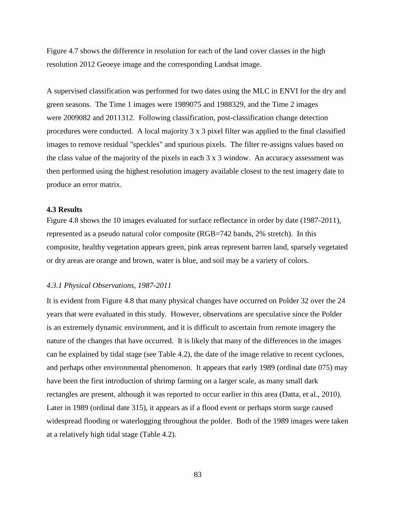
Factors Affecting Drinking Water Security
in South-Western Bangladesh
By
Laura Mahoney Benneyworth, M.S., GISP
Dissertation
Submitted to the Faculty of the
Graduate School of Vanderbilt University
in partial fulfillment of the requirements
for the degree of
DOCTOR OF PHILOSOPHY
in
Interdisciplinary Studies: Environmental Management
August, 2016
Nashville, Tennessee
Approved
Jonathan Gilligan, PhD
Steven Goodbred, PhD
John Ayers, PhD
James H. Clarke, PhD
Page 2
ii
Copyright © 2016 by Laura Mahoney Benneyworth
Page 3
iii
for the children of Bangladesh,
with hope for a brighter future
Page 4
iv
ACKNOWLEDGEMENTS
I would like to thank the Vanderbilt Department of Civil and Environmental Engineering's
Center for Environmental Management Studies (VCEMS) program and Vanderbilt's Earth and
Environmental Sciences Department for their willingness to work together on my behalf to make
this interdisciplinary project possible, and for their educational and financial support. I consider
myself fortunate to have been involved in such an interesting and meaningful project. I am
grateful for the guidance of my advisor, Jonathan Gilligan, and for his patience, kindness and
encouragement. I am also appreciative of Jim Clarke, who provided me with this degree
opportunity, for 30 years of good advice, and for always being my advocate. Steve Goodbred,
John Ayers and Carol Wilson were continually helpful and supportive, and always a pleasure to
work with. I am also thankful for the moral support of my friends and family, and for the
friendship of other graduate students who made my journey a memorable one, including
Bethany, Sandy, Lindsay, Leslie W., Chris T., Greg, Leslie D., Michelle, Laura P., Lyndsey, and
Jenny.
I would also like to extend my sincere gratitude to our Bangladeshi colleagues, for their technical
assistance and their friendship, which made this work possible. Many people participated in the
fieldwork from the University of Khulna, the University of Dhaka, and Pugmark Tours. In
particular, I want to thank my dear and faithful baghni and baghna, Farjana and Zitu; and also
Reza, Babu, Sadam, Matab, Kushal, Dr. Kazi Matin Ahmed, Dr. D. K. Datta, and Bachchu.
Finally, and most importantly, I would like to thank my husband, Al, for his unfailing love and
support, and for always believing in me.
This work was supported by the United States Office of Naval Research under Grant (N00014-
11-1-0683) and conducted in accordance with Institutional Review Board (130235).
Page 5
v
Disclaimer:
This dissertation was prepared as an account of work sponsored by an Agency of the United
States Government. Neither the United States Government nor any agency thereof, nor any of
their employees, makes any warranty, express or implied, or assumes any legal liability or
responsibility for the accuracy, completeness, or usefulness of any information apparatus,
product, or process disclosed, or represents that its use would not infringe privately owned
rights. Reference herein to any specific commercial product, process, or service by trade name,
trademark, manufacturer, or otherwise does not necessarily constitute or imply its endorsement
recommendation, or favoring by the United States Government or any agency thereof.
Page 6
vi
TABLE OF CONTENTS
Page
DEDICATION ............................................................................................................................... iii
ACKNOWLEDGEMENTS ........................................................................................................... iv
LIST OF TABLES ...........................................................................................................................x
LIST OF FIGURES ....................................................................................................................... xi
1 Introduction ...............................................................................................................................1
1.1 Overview ...............................................................................................................................1
1.2 Study Area .............................................................................................................................2
1.3 Research Objectives ..............................................................................................................5
1.4 Structure of Dissertation ........................................................................................................5
1.5 References .............................................................................................................................6
2 Exploring Water Indices and Associated Parameters: A Case Study ..................................9
Abstract .......................................................................................................................................9
2.1 Introduction ...........................................................................................................................9
2.2 Methods ...............................................................................................................................10
2.2.1 Index Descriptions .........................................................................................................11
2.2.1.1 Water Scarcity .........................................................................................................11
2.2.1.2 Water Poverty ..........................................................................................................12
2.2.1.3 Water Vulnerability .................................................................................................13
2.2.1.4 Water Security .........................................................................................................13
Page 7
vii
2.2.2 Parameter and Component Descriptions .......................................................................13
2.2.3 Overview of Analysis ....................................................................................................14
2.3 Results .................................................................................................................................15
2.3.1 Indices............................................................................................................................15
2.3.2 Parameter Values ...........................................................................................................16
2.3.3 Missing Parameters .......................................................................................................21
2.4 Discussion ...........................................................................................................................23
2.5 Conclusions .........................................................................................................................25
2.6 Acknowledgements .............................................................................................................25
2.7 References ...........................................................................................................................26
Appendix: Country Descriptions ...............................................................................................30
Appendix References ................................................................................................................33
3 Drinking Water Insecurity: Water Quality and Access in Coastal South-Western
Bangladesh ....................................................................................................................................35
Abstract .....................................................................................................................................35
3.1 Introduction .........................................................................................................................35
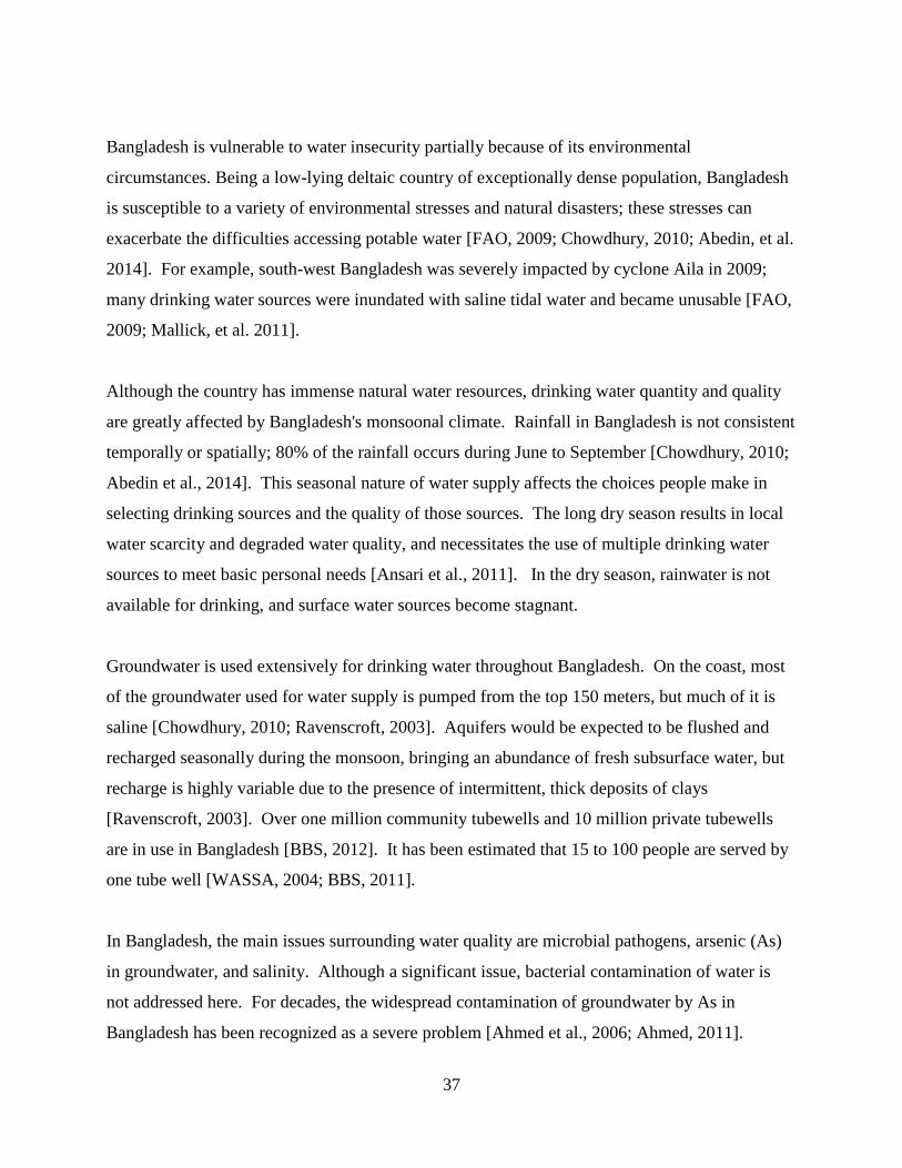
3.1.1 Factors Affecting Water Security in Bangladesh ..........................................................36
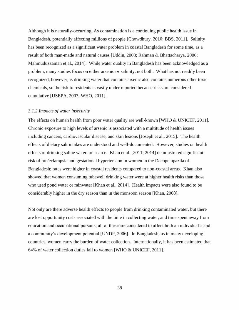
3.1.2 Impacts of Water Insecurity ..........................................................................................38
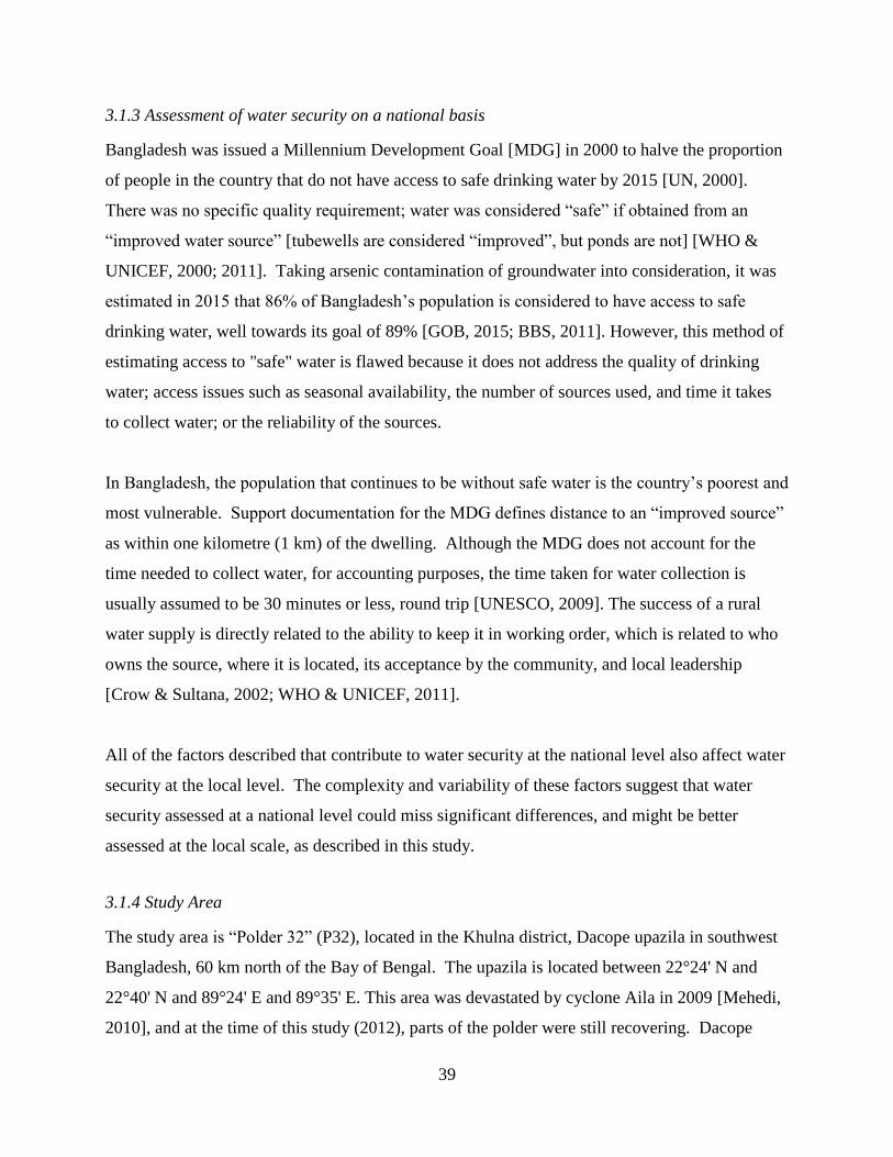
3.1.3 Assessment of Water Security on a National Basis.......................................................39
3.1.4 Study Area .....................................................................................................................39
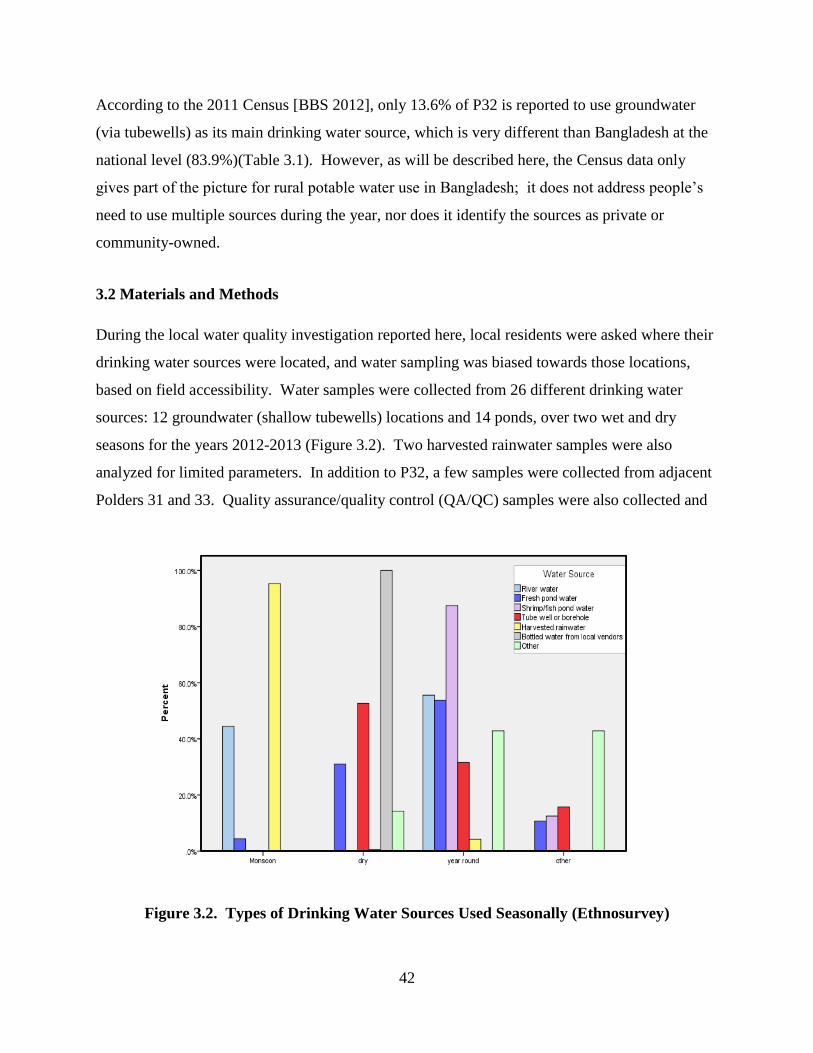
3.2 Materials and Methods ........................................................................................................42
3.3 Results and Discussion ........................................................................................................43
3.3.1 Drinking Water Availability and Accessibility .............................................................44
Page 8
viii
3.3.1.1 Drinking Water Sources and Ownership .................................................................44
3.3.1.2 Non-Drinking Water Uses .......................................................................................44
3.3.1.3 Seasonality ...............................................................................................................44
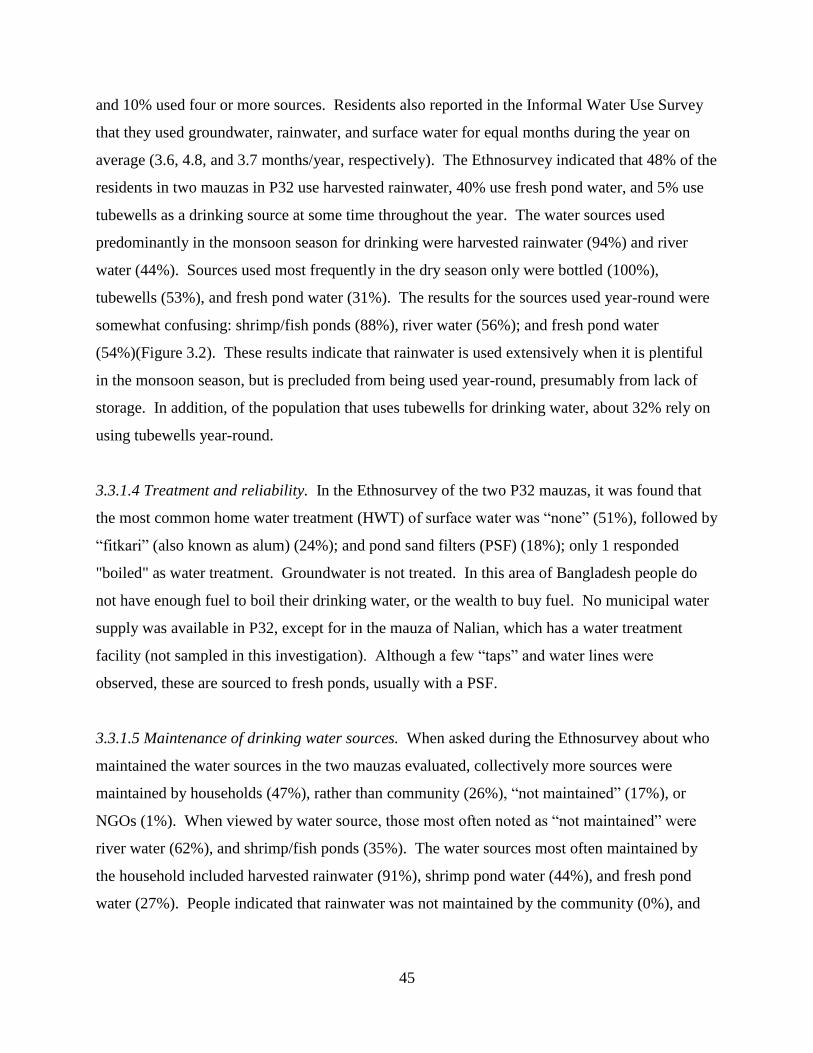
3.3.1.4 Treatment and Reliability ........................................................................................45
3.3.1.5 Maintenance of Drinking Water Sources ................................................................45
3.3.1.6 Water Collection Travel Time, Distance and Gender .............................................46
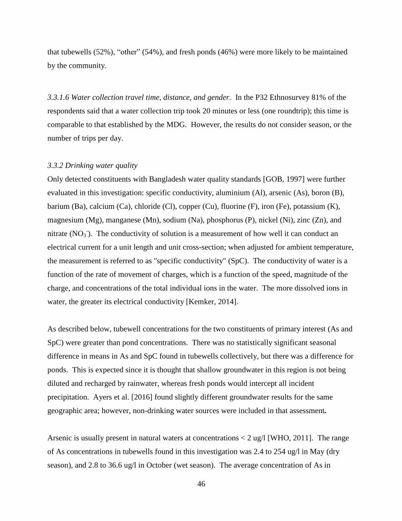
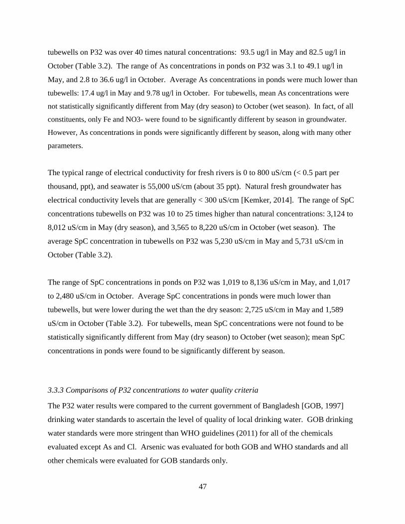
3.3.2 Drinking Water Quality .................................................................................................46
3.3.3 Comparisons of P32 Concentrations to Water Quality Criteria ....................................47
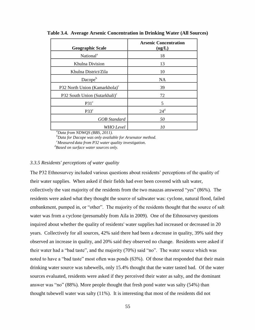
3.3.4 Comparisons of Arsenic Concentrations to National Data............................................50
3.3.5 Residents' Perceptions of Water Quality .......................................................................55
3.3.6 Problems with Potential Mitigation Measures ..............................................................56
3.4 Conclusions .........................................................................................................................57
3.5 Acknowledgements .............................................................................................................58
3.6 References ...........................................................................................................................58
4 Evaluation of Land Use at Polder 32 Using Remote Sensing ..............................................63
4.1 Introduction .........................................................................................................................63
4.1.1 Research Objectives ......................................................................................................69
4.1.2 Use of Remote Sensing to Assess Land Cover Change ................................................70
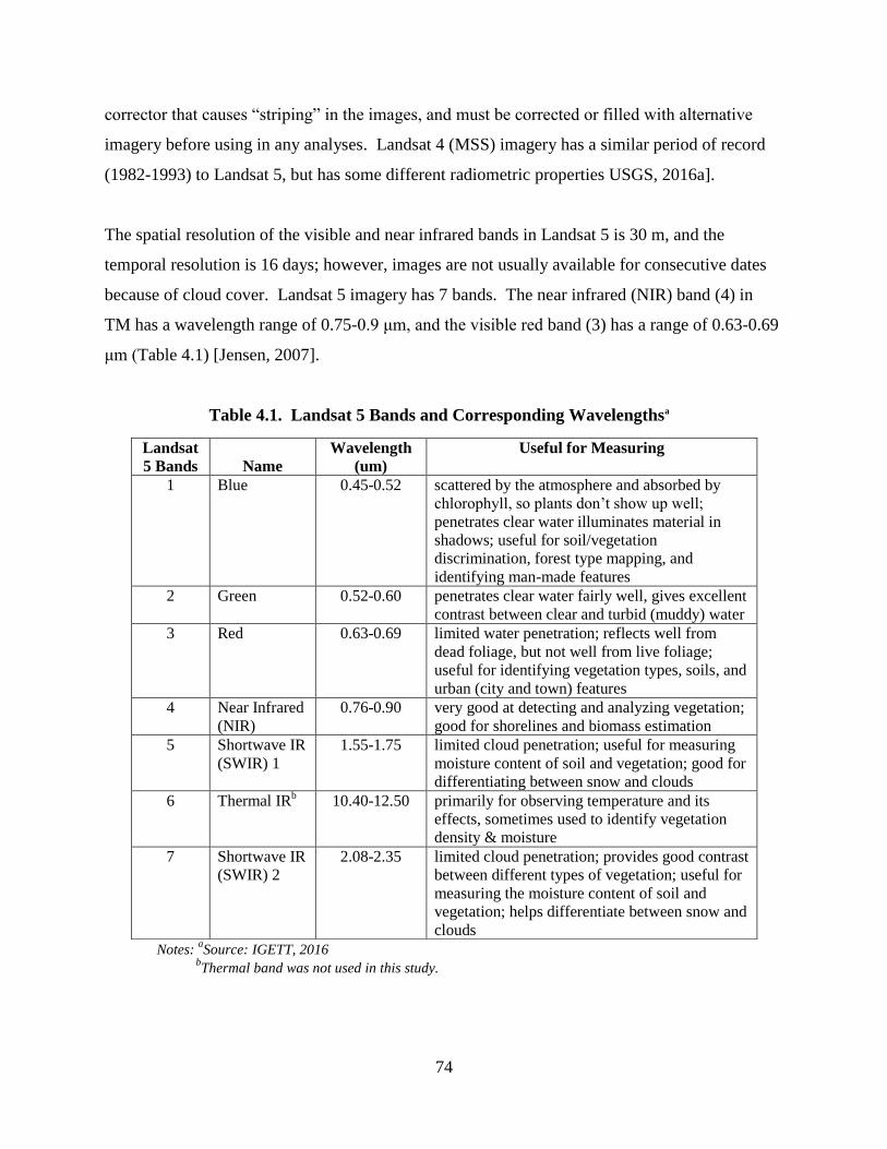
4.1.3 Spectral Characteristics and Indices ..............................................................................72
4.1.4 Landsat Sensor...............................................................................................................73
4.1.5 Image Pre-Processing ....................................................................................................75
4.1.6 Classification and Change Detection .............................................................................76
Page 9
ix
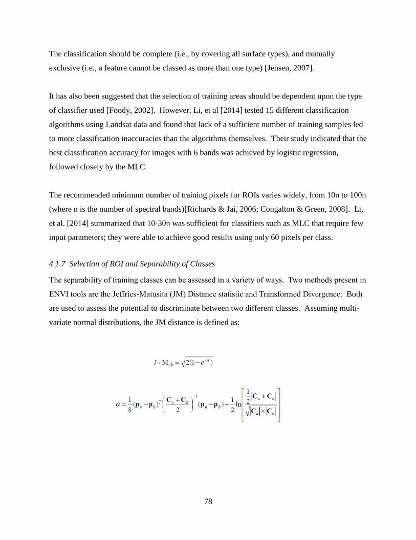
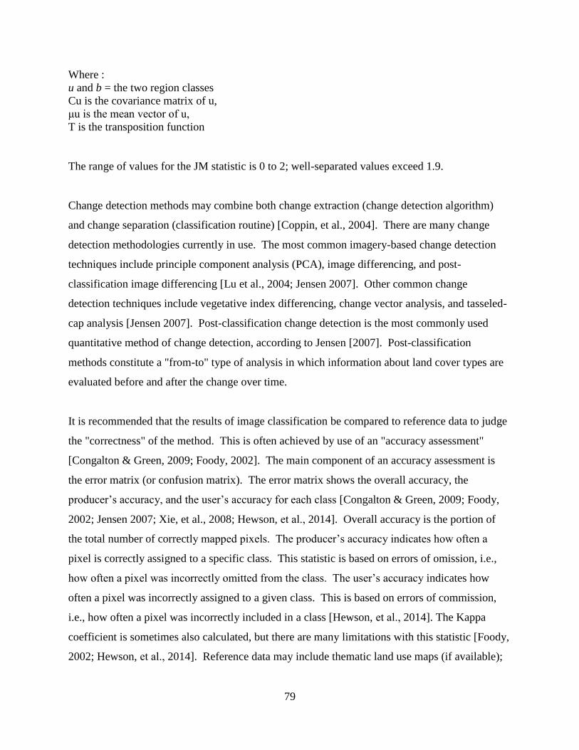
4.1.7 Selection of ROIs and Separability of Classes ..............................................................78
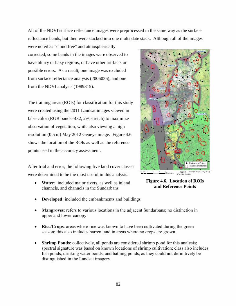
4.2 Materials and Methods ........................................................................................................80
4.3 Results .................................................................................................................................83
4.3.1 Physical Observations, 1987-2011 ................................................................................83
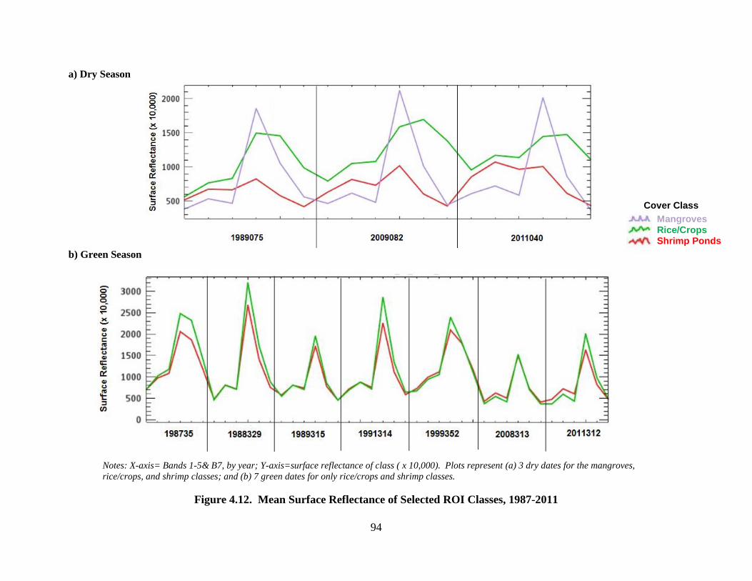
4.3.2 Spectral Signatures and Surface Reflectance ..............................................................92
4.3.3 Selection of ROIs and Separability of Classes ..............................................................95
4.3.4 Classification and Change Detection .............................................................................96
4.3.5 Accuracy Assessment ..................................................................................................100
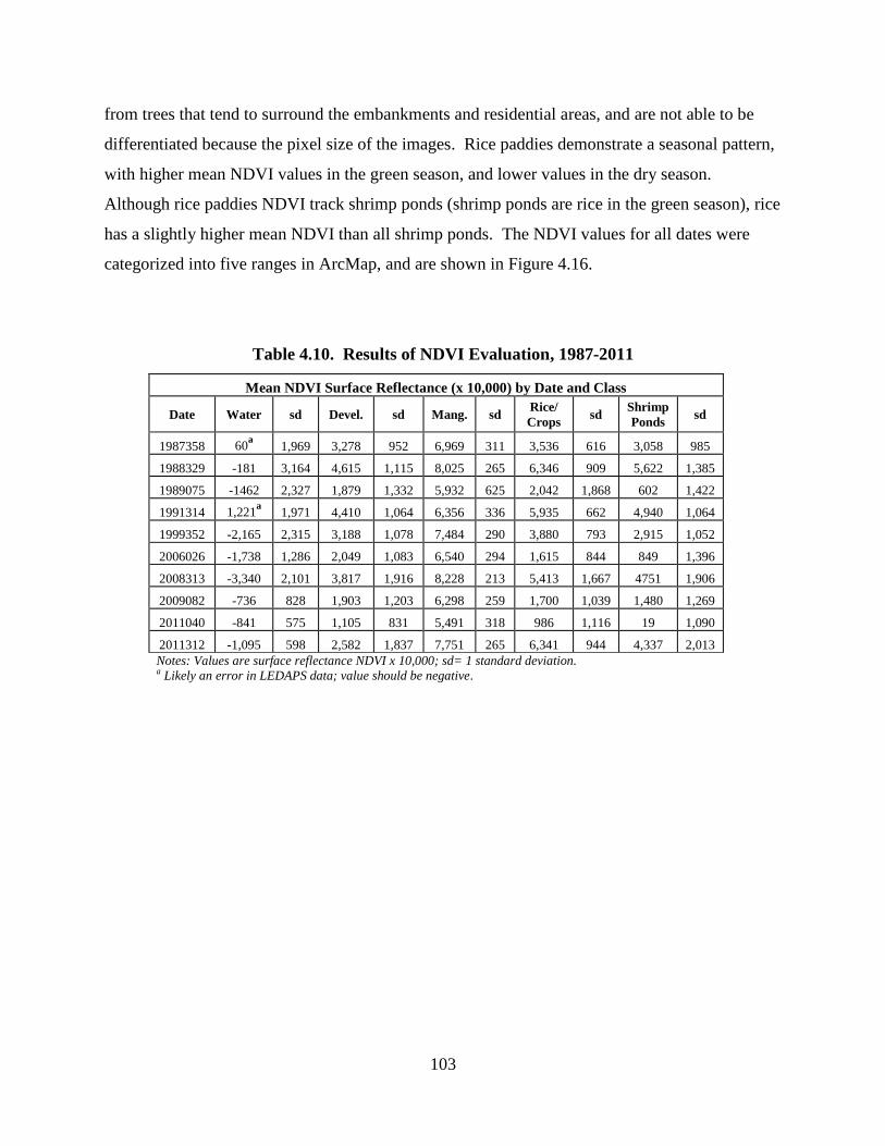
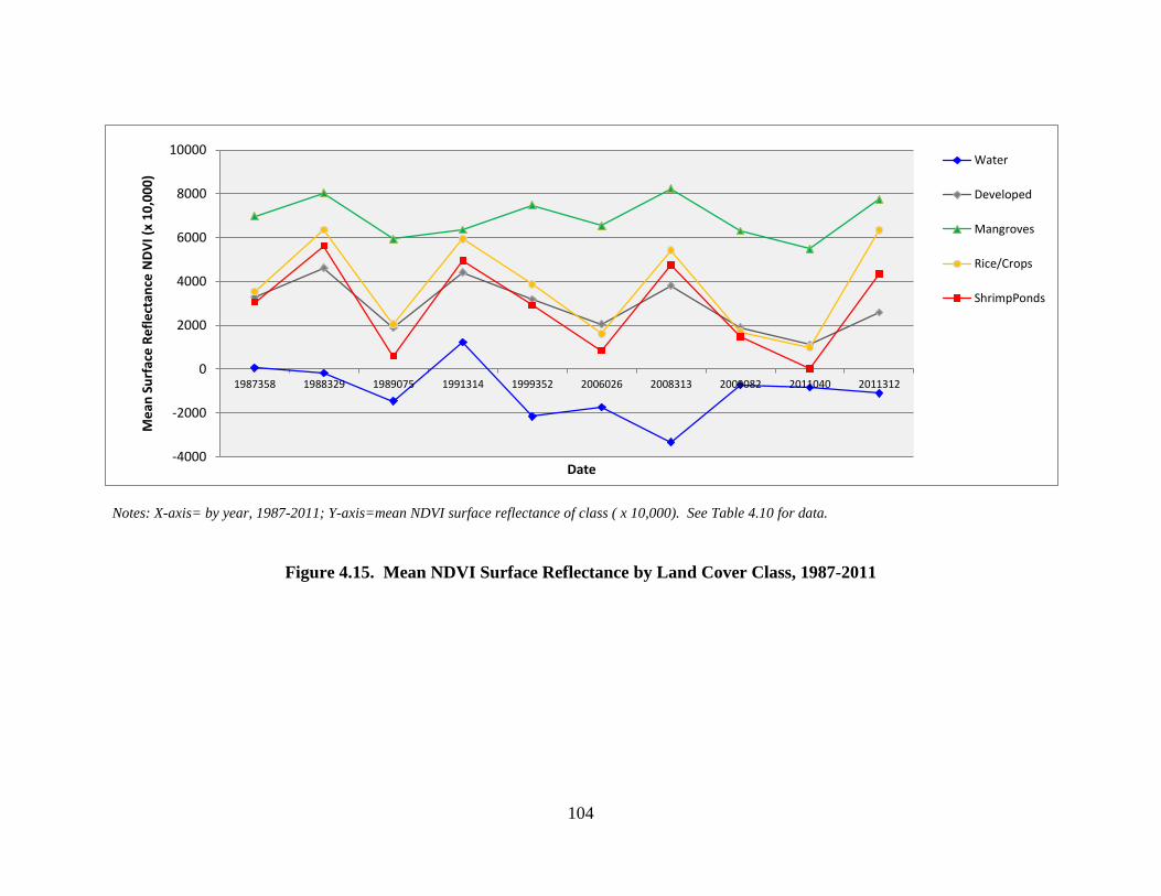
4.3.6 NDVI Surface Reflectance ..........................................................................................102
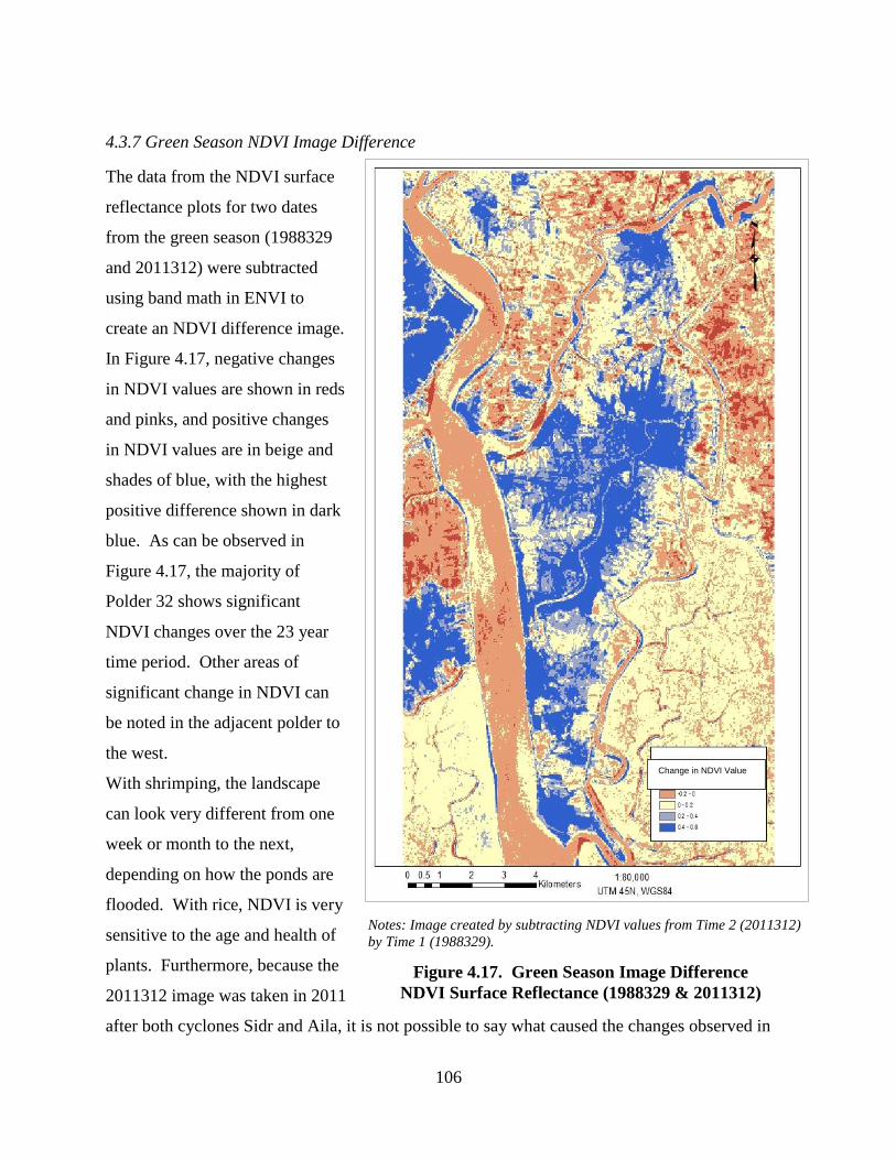
4.3.7 Green Season NDVI Image Difference .......................................................................106
4.4 Discussion and Conclusions ..............................................................................................107
4.4.1 Summary......................................................................................................................107
4.4.2 Discussion and Conclusions ........................................................................................109
4.4.3 Limitations ...................................................................................................................110
4.5 References .........................................................................................................................112
5 Summary ................................................................................................................................117
5.1 Research Contributions .....................................................................................................117
5.2 Potential Future Work .......................................................................................................118
APPENDIX
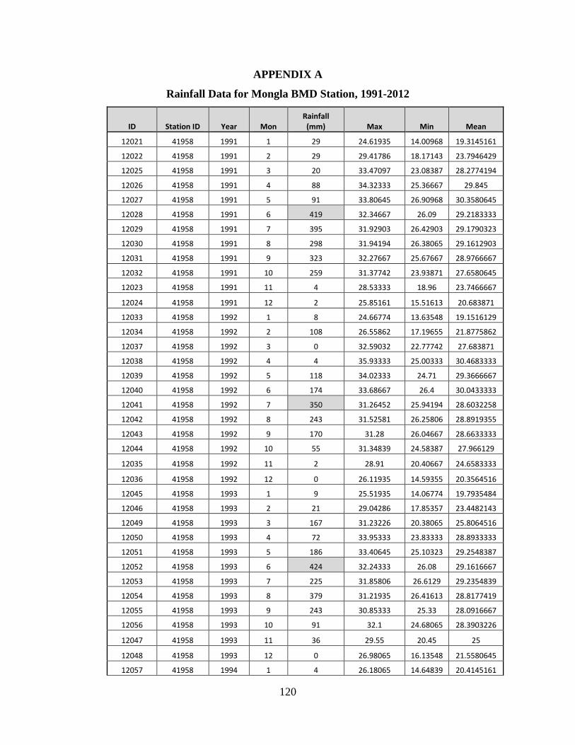
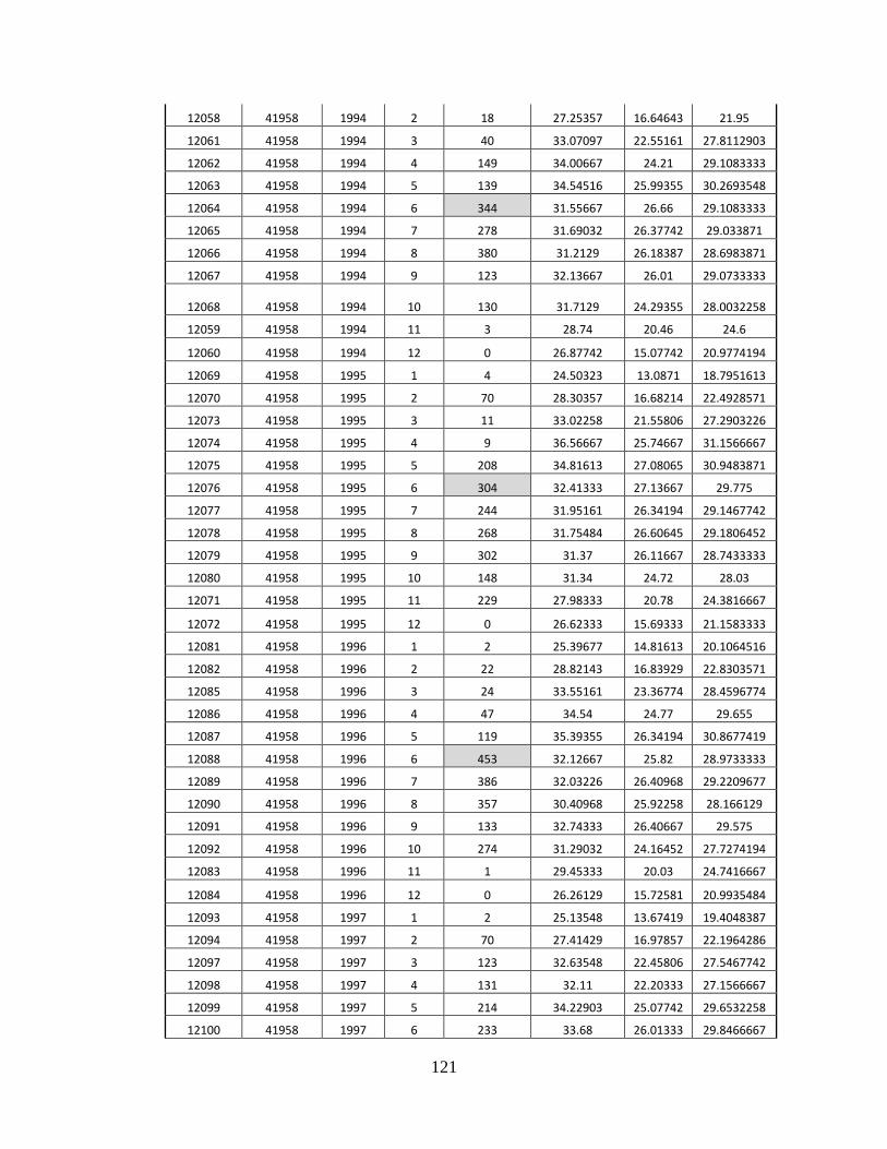
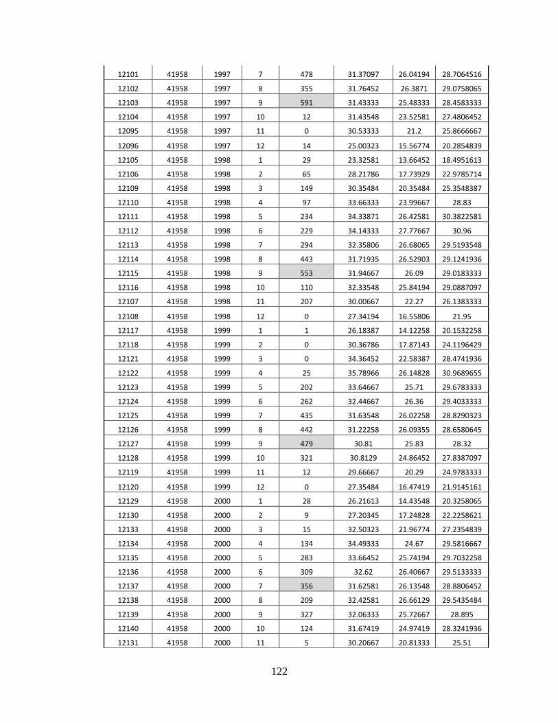
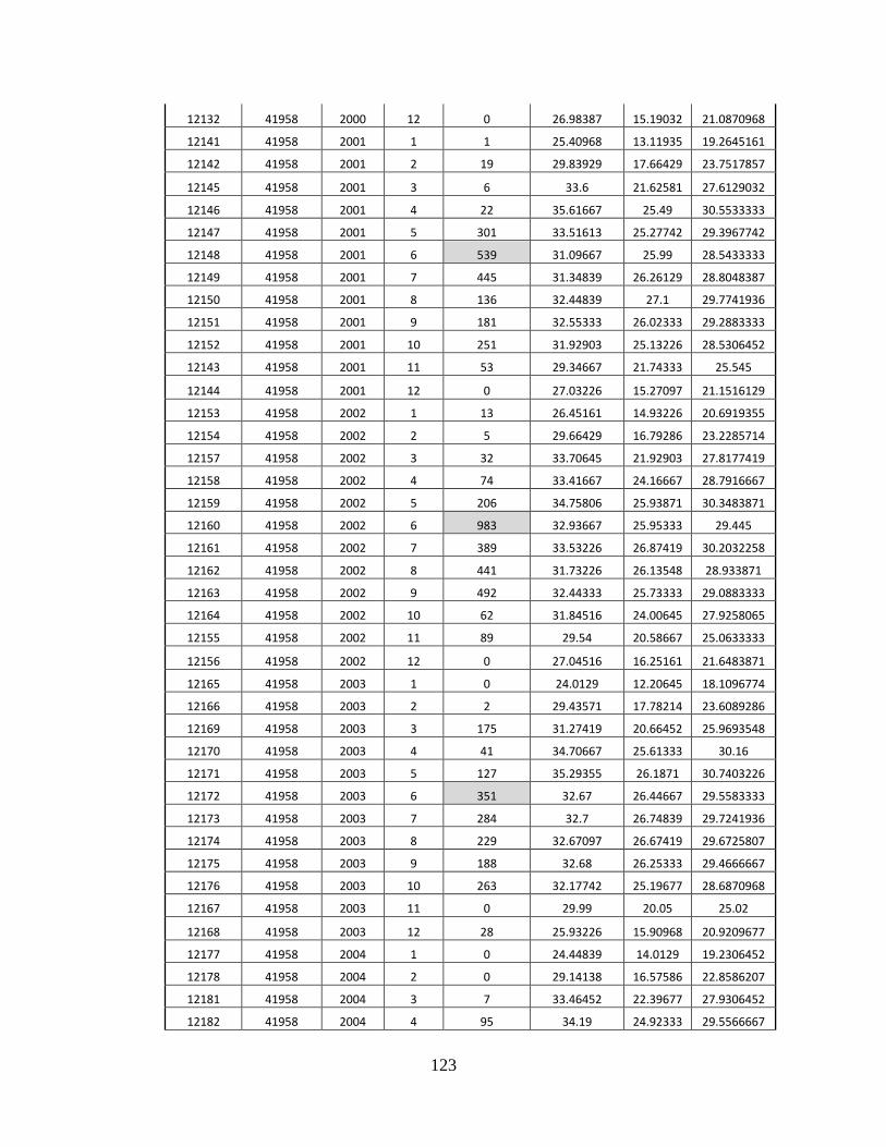
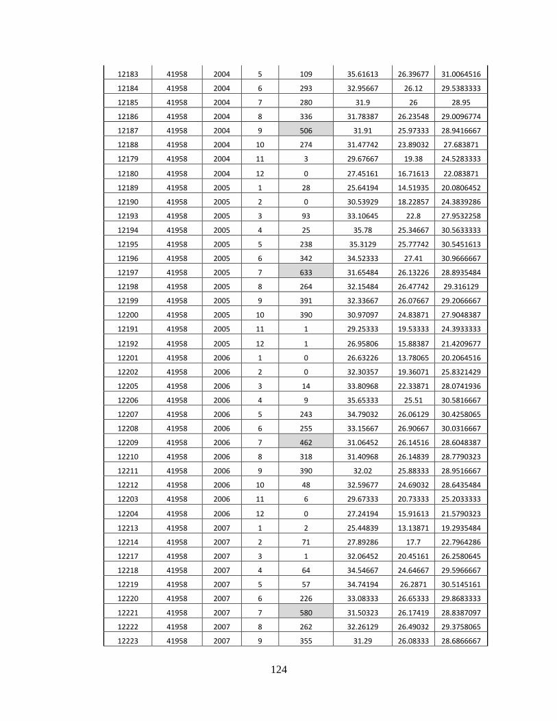
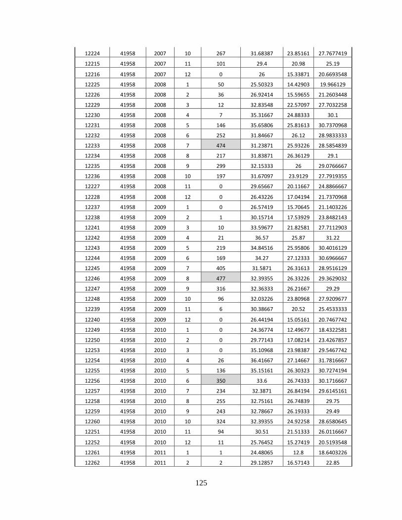
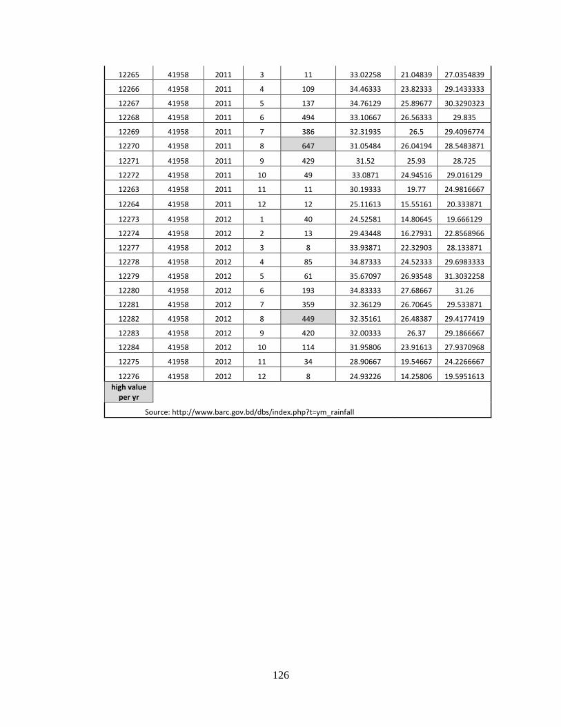
A. Rainfall Data for Mongla BMD Station, 1991-2012 ...............................................................120
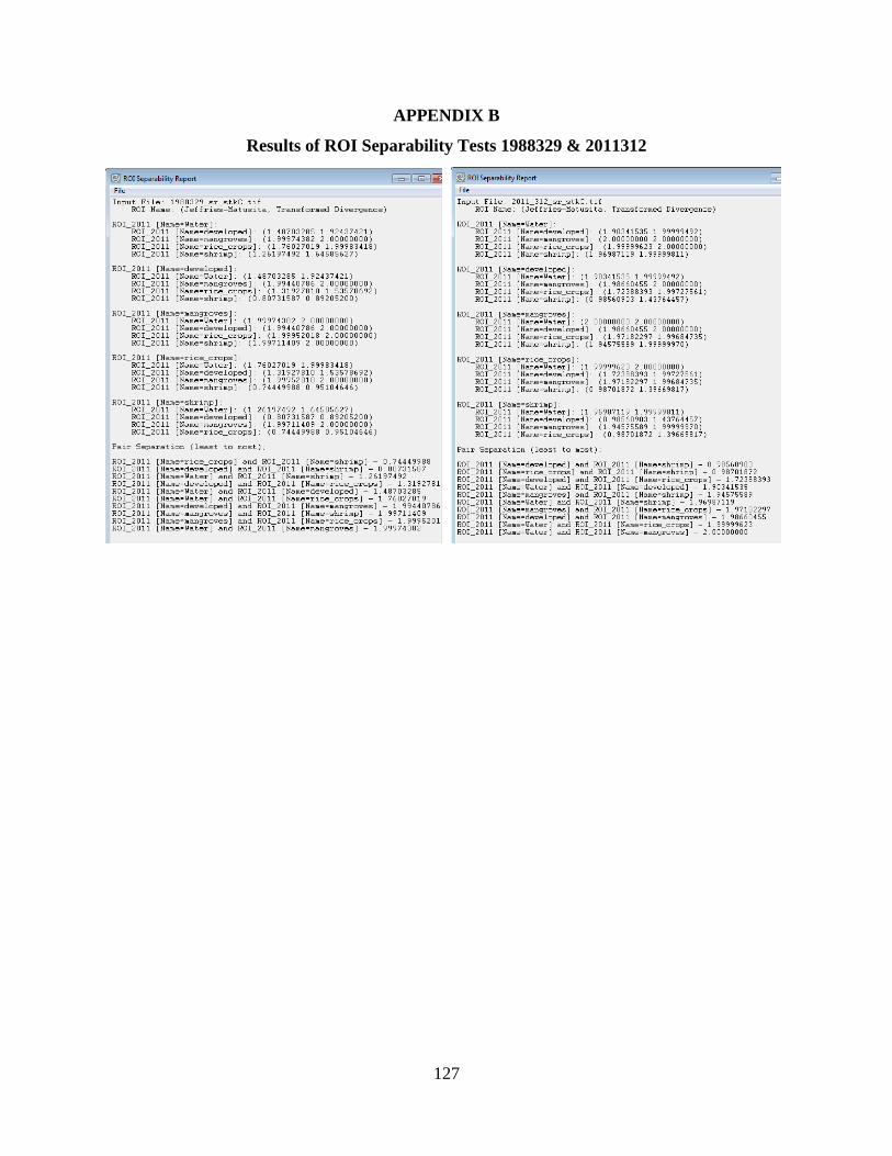
B. Results of ROI Separability Tests 1988329 & 2011312 .........................................................127
Page 10
x
LIST OF TABLES
Table Page
2.1 Indices for Bangladesh and Sri Lanka ....................................................................................15
2.2 Water Index Parameter Values for Bangladesh and Sri Lanka................................................18
2.3 Missing Parameters ..................................................................................................................22
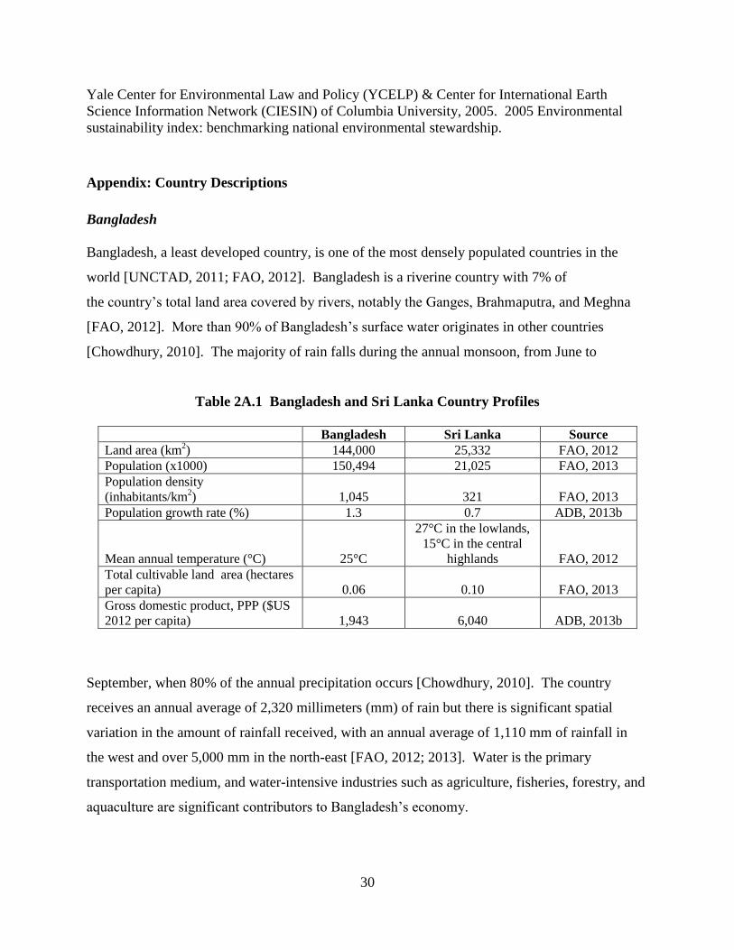
2.A.1 Bangladesh and Sri Lanka Country Profiles ........................................................................30
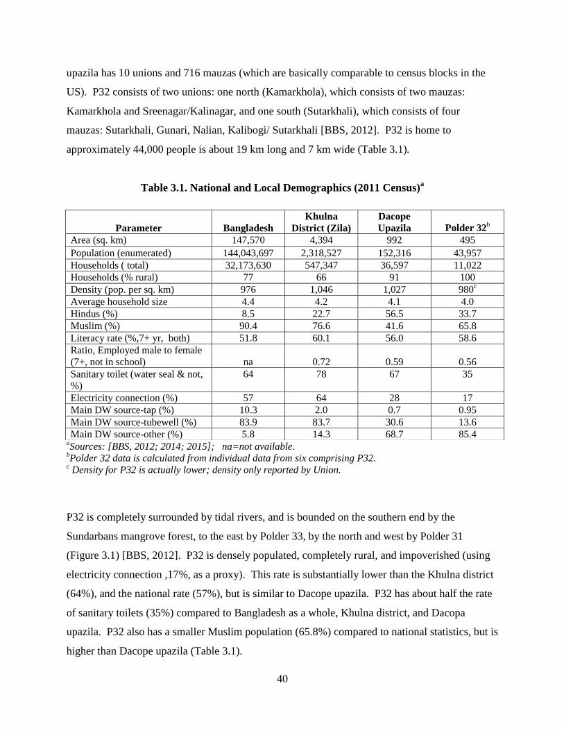
3.1 National and Local Demographics (2011 Census) ..................................................................40
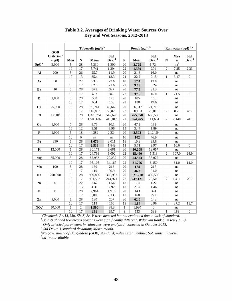
3.2 Averages of Drinking Water Sources Over Dry and Wet Seasons, 2012-2013 ......................48
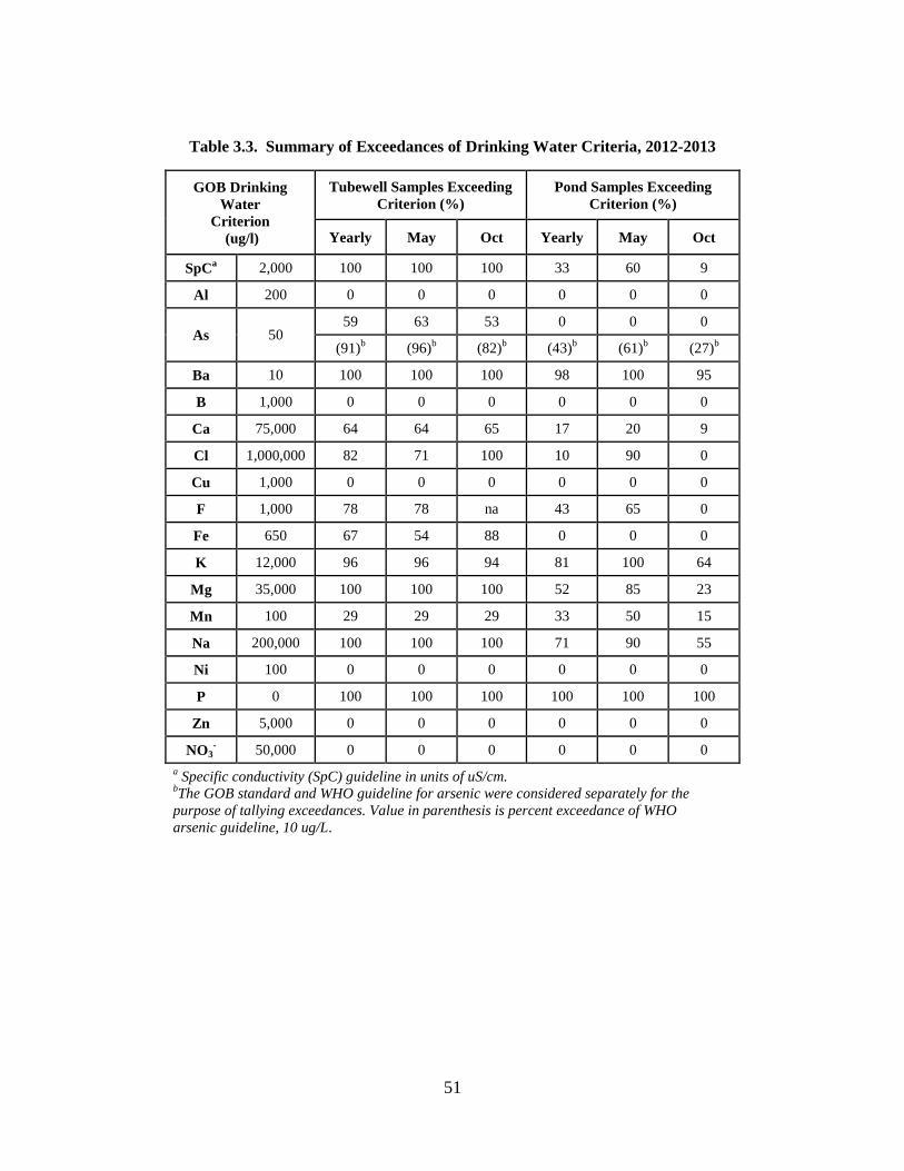
3.3 Summary of Exceedances of Drinking Water Criteria, 2012-2013 ..................................................51
3.4 Average Arsenic Concentration in Drinking Water (All Sources) ..........................................55
4.1 Landsat 5 Bands and Corresponding Wavelengths .................................................................74
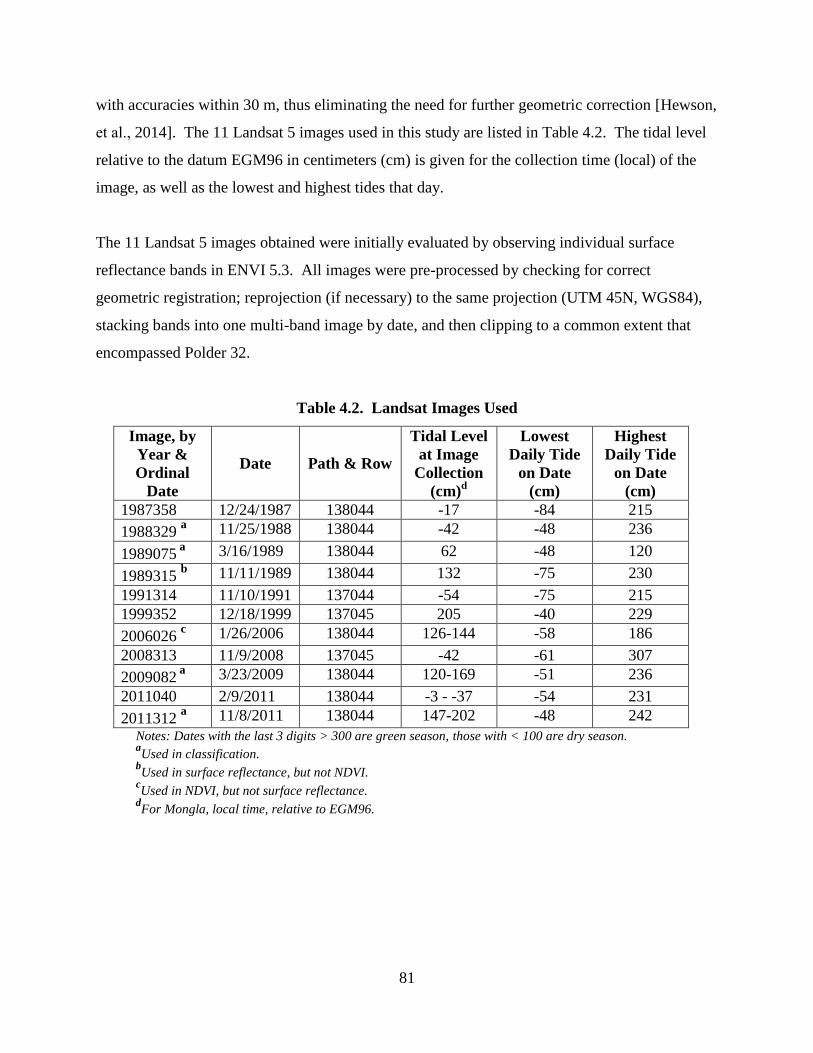
4.2 Landsat Images Used ...............................................................................................................81
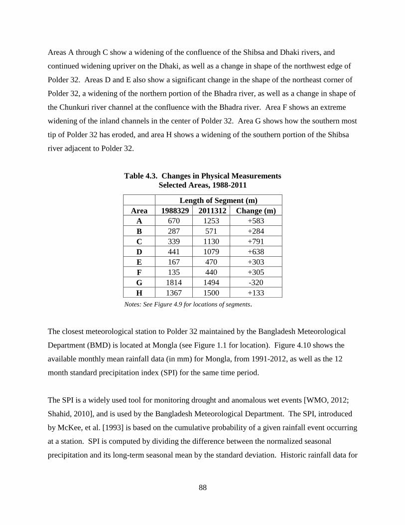
4.3 Changes in Physical Measurements in Selected Areas, 1988-2011 ........................................88
4.4 SPI Categories ..........................................................................................................................89
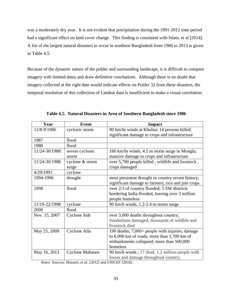
4.5 Natural Disasters in Area of Southern Bangladesh since 1986 ...............................................91
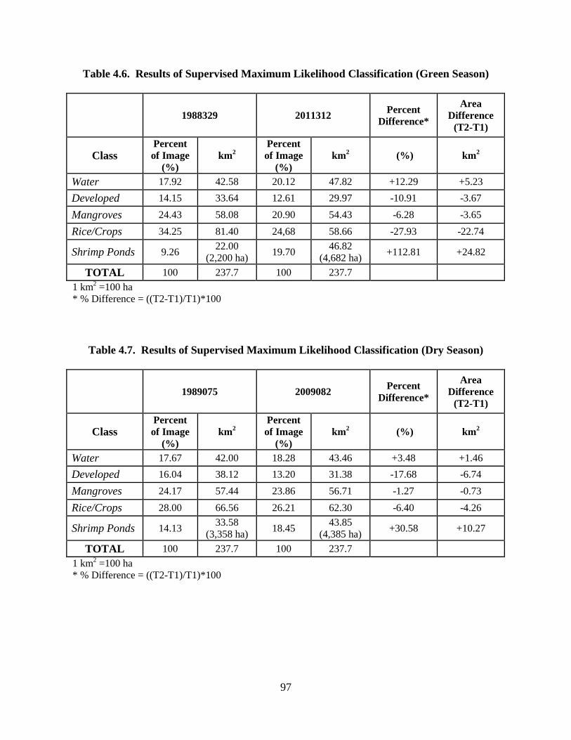
4.6 Results of Supervised Maximum Likelihood Classification (Green Season) ..........................97
4.7 Results of Supervised Maximum Likelihood Classification (Dry Season) .............................97
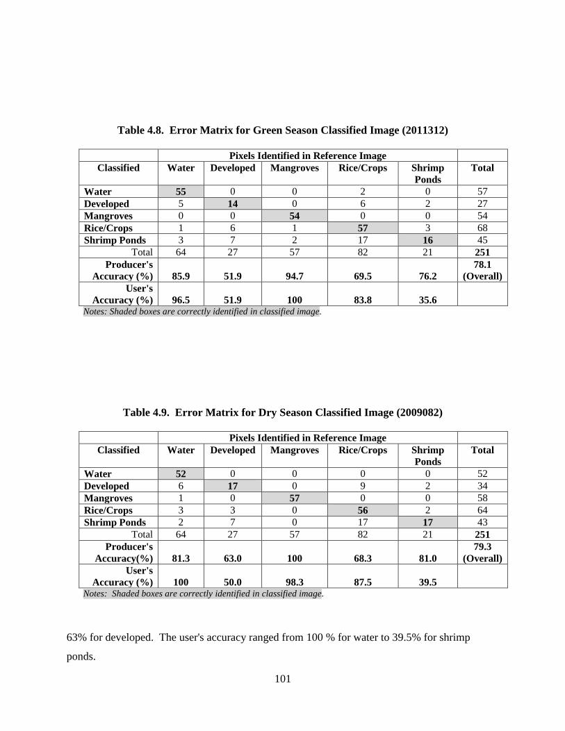
4.8 Error Matrix for Green Season Classified Image (2011312) .................................................101
4.9 Error Matrix for Dry Season Classified Image (2009082) ....................................................101
4.10 Results of NDVI Evaluation, 1987-2011 .............................................................................103
Page 11
xi
LIST OF FIGURES
Figure Page
1.1 Location of Study Area ..............................................................................................................4
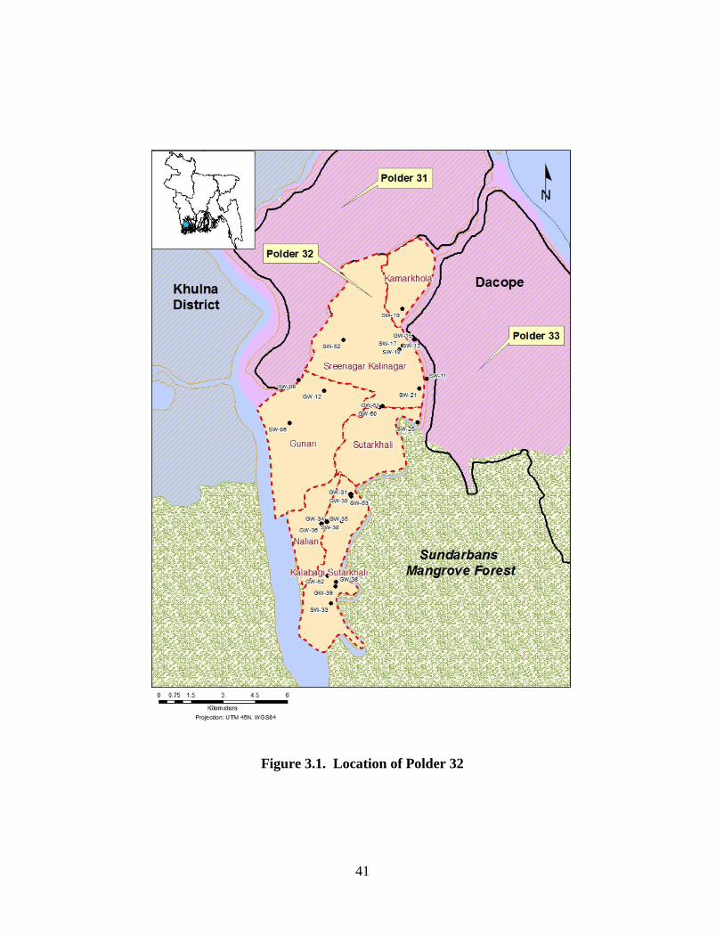
3.1 Location of Polder 32...............................................................................................................41
3.2 Types of Drinking Water Sources Used Seasonally (Ethnosurvey) ........................................42
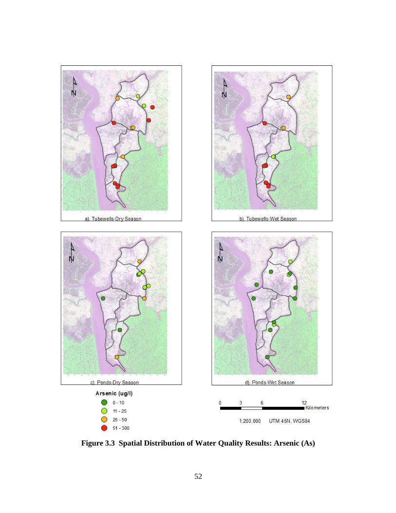
3.3 Spatial Distribution of Water Quality Results: Arsenic (As)...................................................52
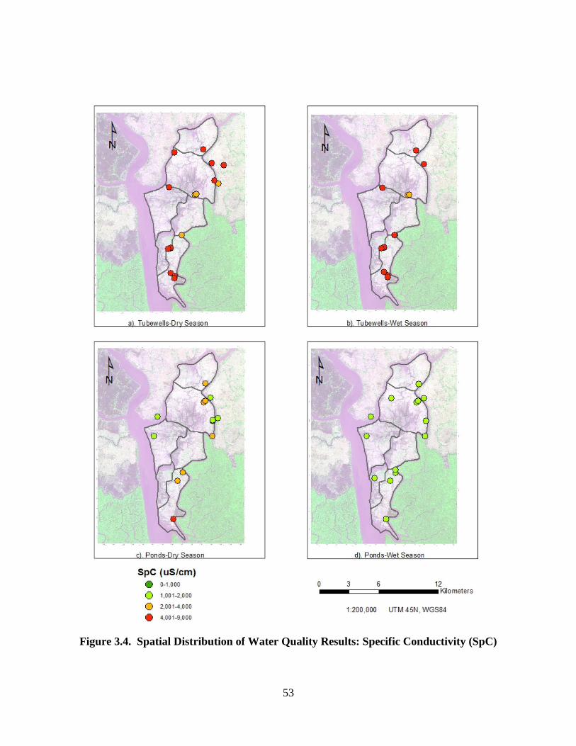
3.4 Spatial Distribution of Water Quality Results: Specific Conductivity (SpC)..........................53
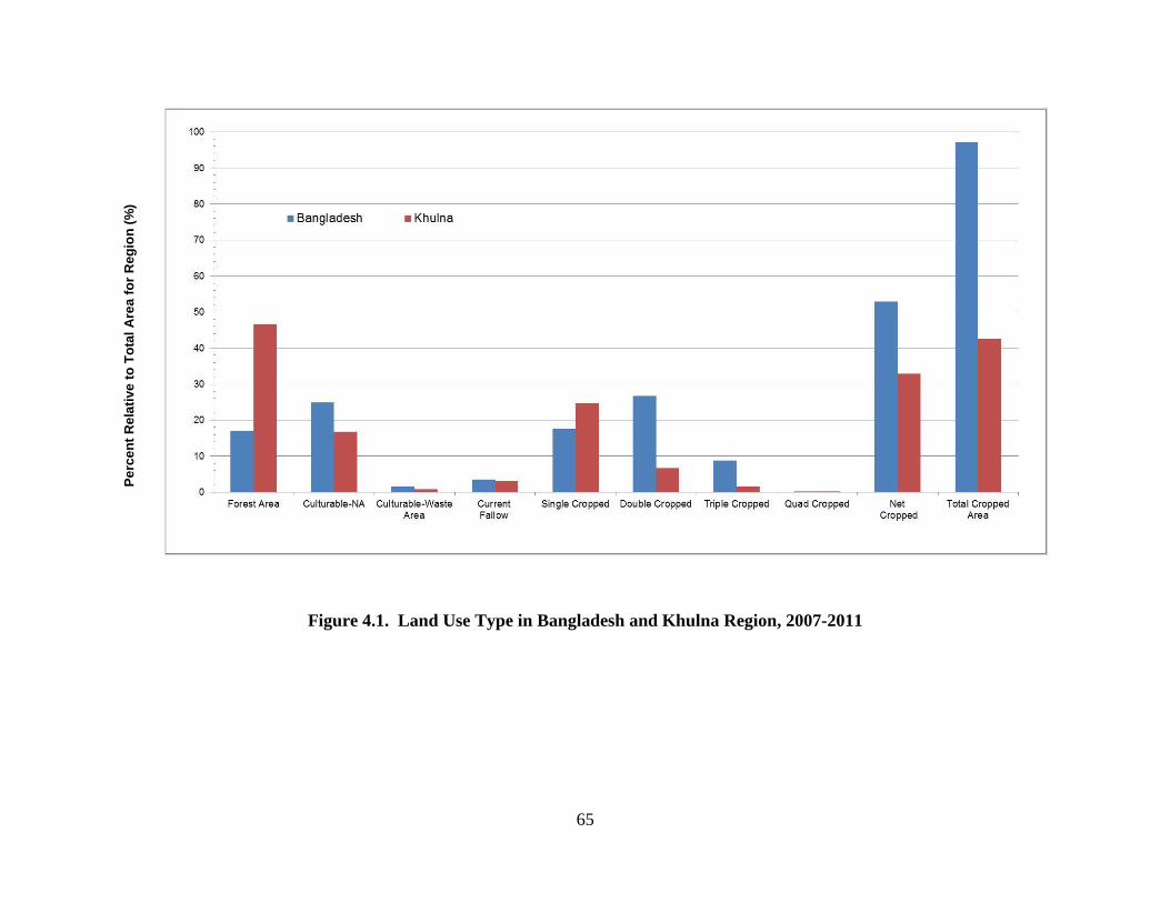
4.1 Land Use Type in Bangladesh and Khulna Region, 2007-2011 ..............................................65
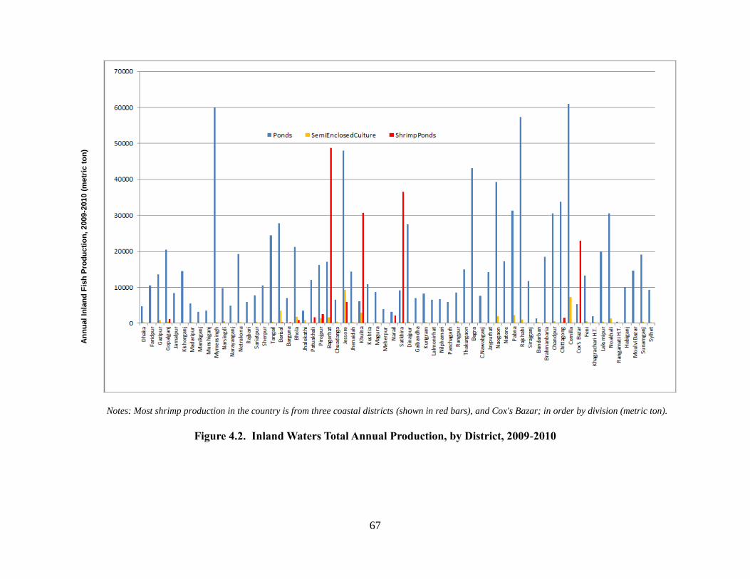
4.2 Inland Waters Total Annual Production, by District, 2009-2010 .............................................67
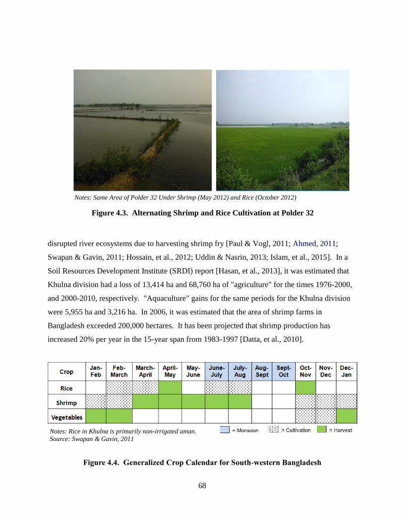
4.3 Alternating Shrimp and Rice Cultivation at Polder 32 ............................................................68
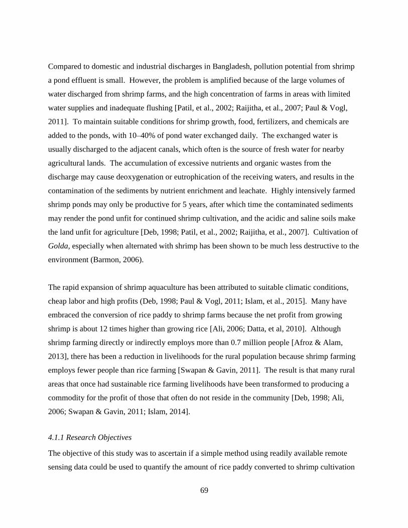
4.4 Generalized Crop Calendar for South-Western Bangladesh ....................................................69
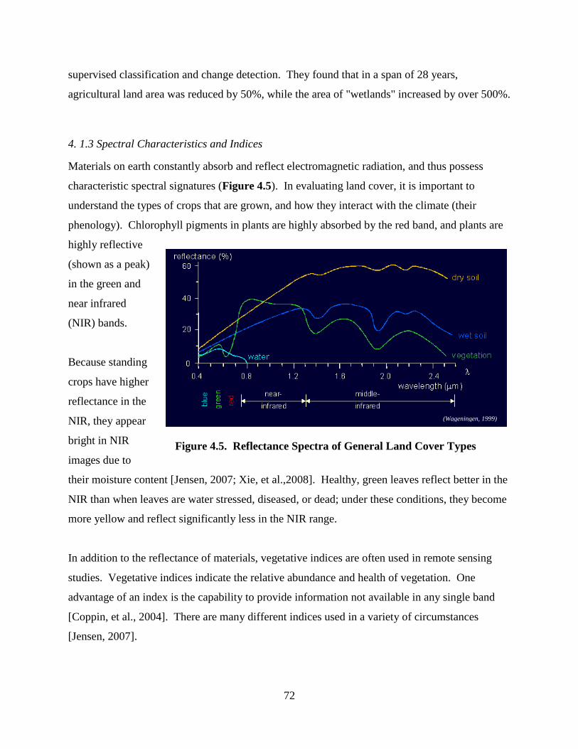
4.5 Reflectance Spectra of General Land Cover Types .................................................................72
4.6 Location of ROIs and Reference Points ...................................................................................82
4.7 Examples of the Five Classes and Representation in Imagery ................................................84
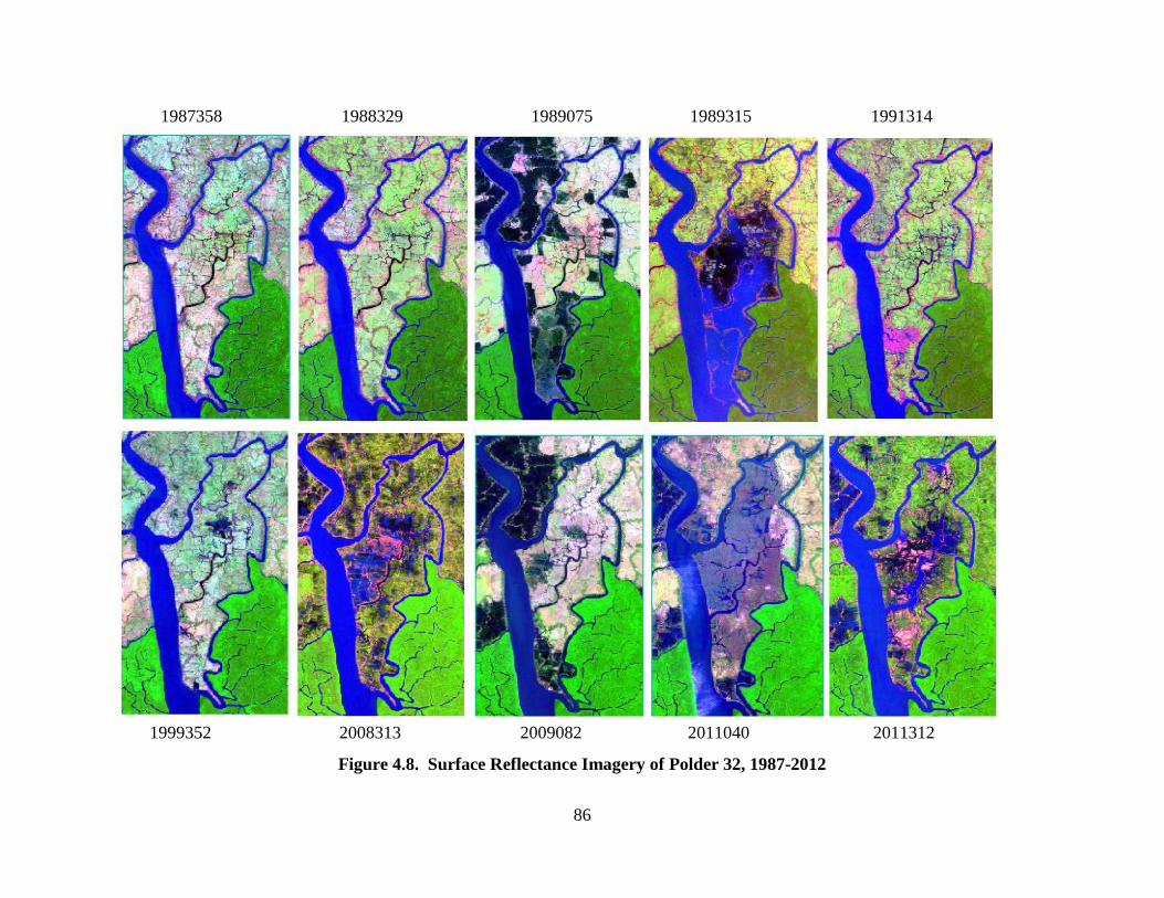
4.8 Surface Reflectance Imagery of Polder 32, 1987-2012 ...........................................................86
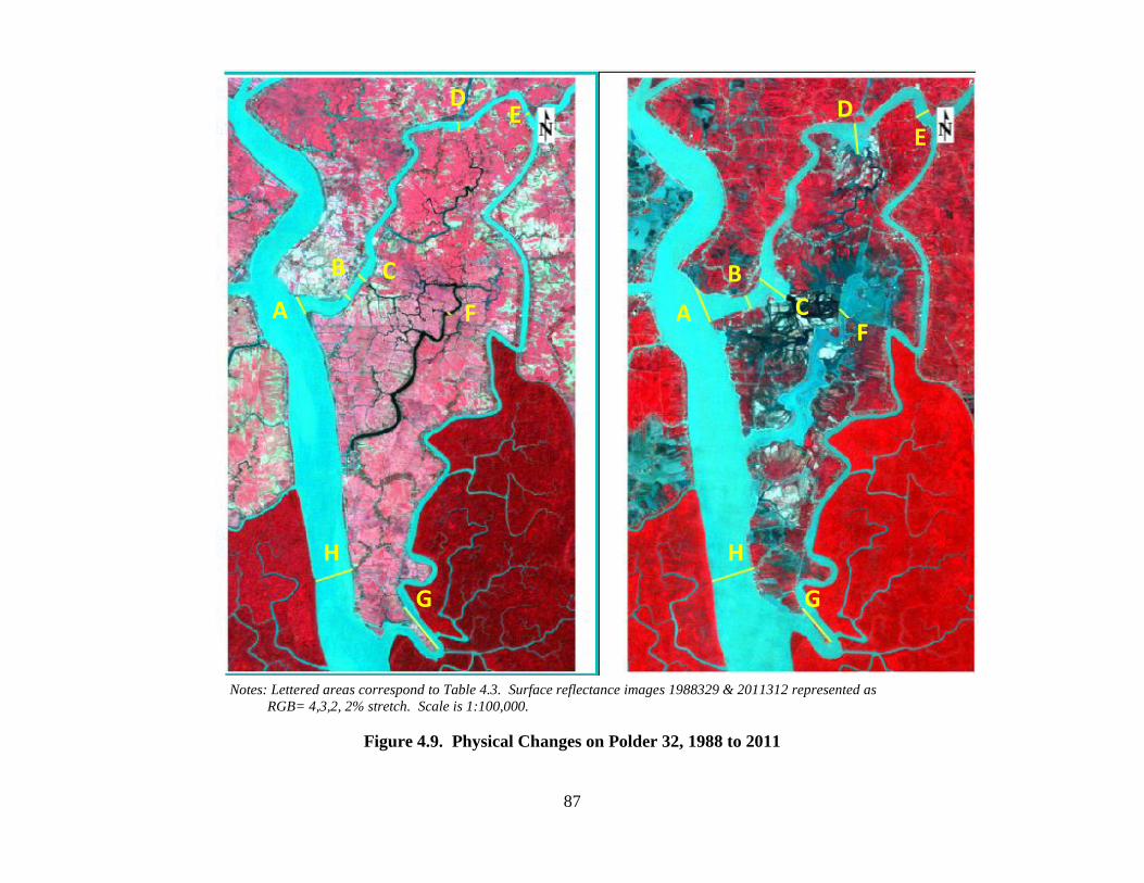
4.9 Physical Changes on Polder 32, 1988 -2011 ...........................................................................87
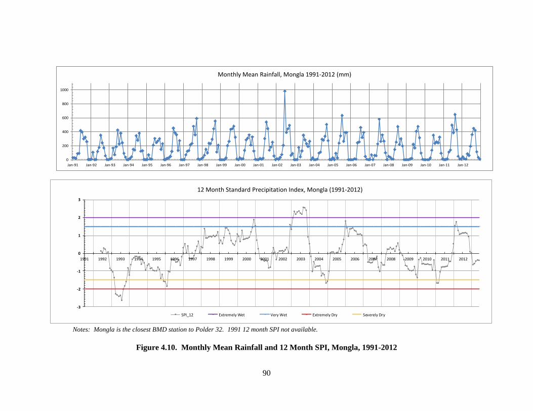
4.10 Monthly Mean Rainfall and 12 Month SPI, Mongla, 1991-2012 ..........................................90
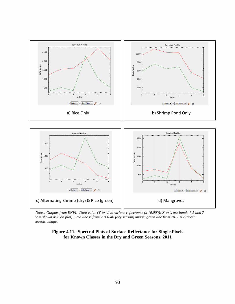
4.11 Spectral Plots of Surface Reflectance for Single Pixels for Known Classes, Dry and Green
Seasons, 2011 .................................................................................................................................93
4.12 Mean Surface Reflectance of Selected ROI Classes, 1987-2011 ..........................................94
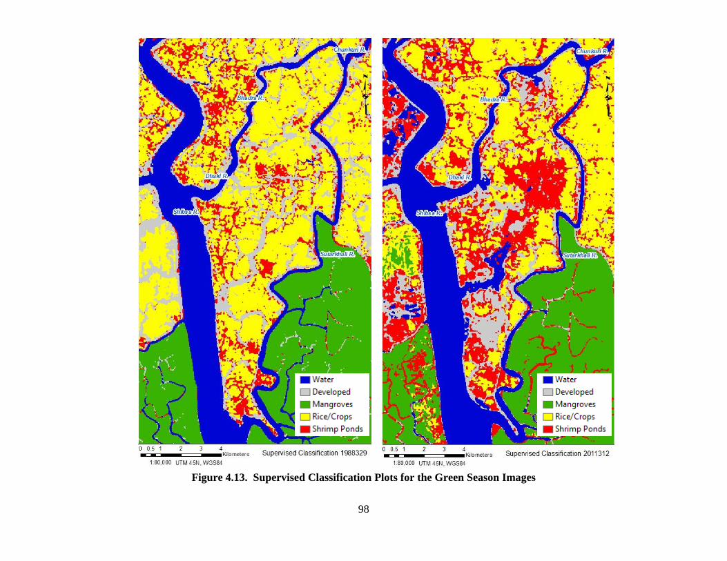
4.13 Supervised Classification Plots for the Green Season Images ...............................................98
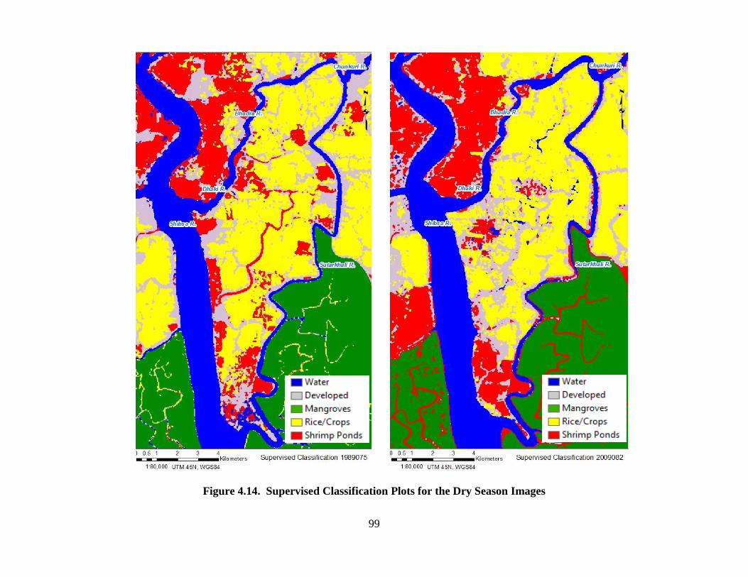
4.14 Supervised Classification Plots for the Dry Season Images ..................................................99
4.15 Mean NDVI Surface Reflectance by Land Cover Class, 1987-2011 ..................................104
Page 12
xii
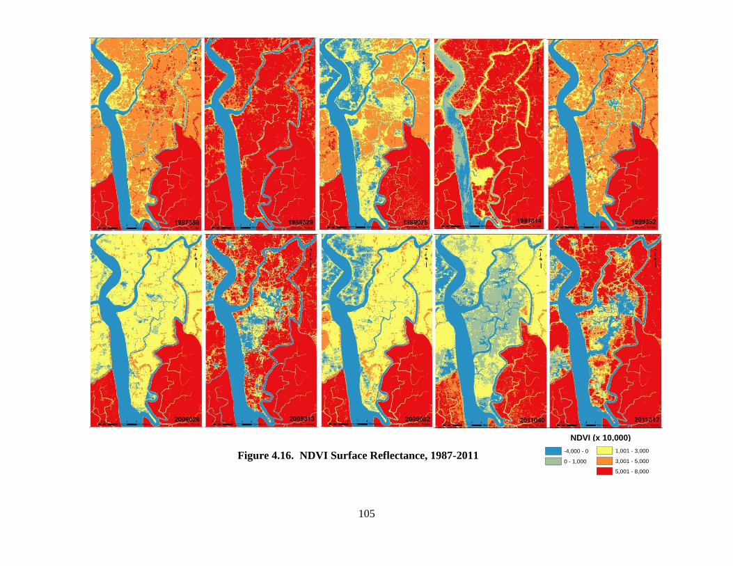
4.16 NDVI Surface Reflectance, 1987-2011 ...............................................................................105
4.17 Green Season Image Difference NDVI Surface Reflectance (1988329&201131) .............106
Page 13
1
CHAPTER 1
Introduction
1.1 Overview
In the past century, rates of water usage have grown twice as rapidly as global population [FAO
2007; UN, 2013]. Although global renewable freshwater resources are currently sufficient to
meet population requirements, uneven distribution of water resources, compounded by pollution
and mismanagement, results in severe national and regional disparities in water availability and
quality [UN, 2013]. These circumstances bring into question the state of water security from a
global perspective down to the individual level. There are many definitions of water security,
but this is one of the most comprehensive:
‘the capacity of a population to safeguard sustainable access to adequate quantities of
acceptable quality water for sustaining livelihoods, human well-being, and socio-economic
development, for ensuring protection against water-borne pollution and water-related
disasters, and for preserving ecosystems in a climate of peace and political stability’ [UN-
Water, 2013, p. 1].
Water security is a diverse topic, partially because of the wide range of scales at which it is
relevant, and the units of analysis that are necessary [Wouthers, 2010; Cook & Bakker, 2012].
Information about water security is also difficult to synthesize because of the various scales of
data collection. Different disciplines studying water security tend to use different scales, e.g.,
hydrologists focus on watersheds, and social scientists study communities [Cook & Bakker,
2012].
Water security assessed at the national level is inconsistent with the fact that most water
management is conducted at the basin level or lower [Lautze & Manthrithilake ,2012]; what
Bakker [2012] calls the “scalar mismatch”. Bakker [2012] further states that most of the
academic research to date on water security has been poorly integrated with the needs of water
practitioners and policy makers, and thus changes are required for research to make a meaningful
contribution to the global water crisis. Bakker [2012] opines that analysis in the field of water
Page 14
2
security “…requires interdisciplinary, collaborative research, transcending ‘broad’ versus
‘narrow’ and ‘academic’ versus ‘applied’ distinctions…” [p. 915].
1.2 Study Area
Bangladesh provides an acutely relevant area in which to study water security, due to its many
developmental and environmental challenges. Bangladesh is the largest of the “least developed
countries”, and is one of the world’s most densely populated and impoverished countries
[Ravenscroft, 2003]. As such, it is encumbered with the associated strains on its natural
resources. Bangladesh is primarily rural and agricultural, and is one of the world’s most rapidly
growing countries [Ravenscroft, 2003; FAO, 2013].
Bangladesh is a low lying deltaic nation, located in one of the world’s largest floodplains: that of
the Ganges, Brahmaputra, and Meghna rivers [Ravenscroft, 2003; FAO, 2013]. Bangladesh is
extremely vulnerable to water shocks, including floods, cyclones and storm surges [van
Schendel, 2009; FAO, 2009]. Water plays an essential role in the lives of many people in
Bangladesh, especially in rural areas; water is intrinsically linked to livelihoods in agriculture,
fisheries, navigation, forestry, and aquaculture [Ravenscroft, 2003; FAO, 2013]. More than 90%
of Bangladesh’s surface water originates in other countries, which inhibits the country’s ability
to manage its rivers at the watershed level [Chowdhury, 2010]. There is only one multi-purpose
dam in the country, and three barrages exist that are used for irrigation. In addition, India
controls flow from the Ganges River into Bangladesh by means of the Farraka Barrage, which is
under a transboundary treaty for its flow rate during the dry season [FAO, 2013].
Bangladesh has a tropical monsoonal climate; the monsoon ensures plentiful rainfall, but only for
a few months of the year (June-September), when most of the yearly precipitation occurs [FAO,
2009; Chowdhury, 2010; K. Ahmed, 2011] The spatial distribution of rainfall is highly variable
throughout the country, and there is insufficient storage throughout the country to meet the needs
of people and agriculture during the dry season [Ravenscroft, 2003, FAO, 2009; Ansari, et al.,
2011; K. Ahmed, 2011; FAO, 2013]. Approximately 80% of the total water withdrawal in
Bangladesh is from groundwater, with agriculture comprising the greatest sector water
withdrawal (88%) [FAO, 2013]. Lack of safe drinking water is of primary concern in
Page 15
3
Bangladesh due to microbial surface water contamination, as well as the presence of arsenic and
salinity in groundwater wells [Ravenscroft, 2003; Ahmed, et al., 2004; 2011 ; Chowdhury, 2010,
Khan & Kumar, 2010; Mondal, et al., 2013; FAO, 2013].
Rice cultivation is the most important activity in the nation’s economy, and one of the biggest
uses of water [FAO, 2013; Chowdhury, 2010]. The use of groundwater for irrigation has
become increasingly important due to demand for irrigation during the dry season, and the
limited availability of surface water [Ravenscroft, 2003; FAO, 2013].
An important part of the water infrastructure system is the coastal embankment program in the
south-west portion of the country, initiated in the 1960s. Embankments were constructed to
increase agricultural production, to protect agricultural land (polders) from floodwaters, and to
reduce risks to people from water-related hazards [Islam, 2006; A. Ahmed, 2011; FAO, 2013;
Auerbach, et al., 2015]. Although the embankments have led to increased agricultural
production, over time they have also contributed to significant adverse impacts to the
environment [Mondal, et al., 2013; Auerbach, et al., 2015; Rasul & Chowdhury, 2010]. Most of
the southern coast is within 1 to 3 m of the mean sea level [Mondal, et al., 2013]. Due to its low
elevation and flat topography, potential climate change impacts, especially sea level rise, are of
great concern in Bangladesh [FAO, 2009; Chowdhury, 2010; Mondal, et al., 2013].
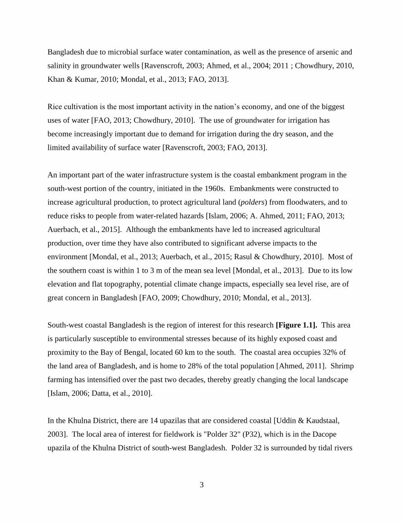
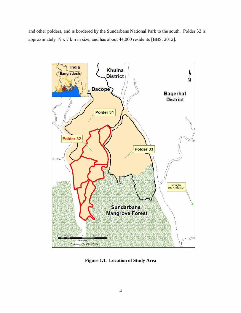
South-west coastal Bangladesh is the region of interest for this research [Figure 1.1]. This area
is particularly susceptible to environmental stresses because of its highly exposed coast and
proximity to the Bay of Bengal, located 60 km to the south. The coastal area occupies 32% of
the land area of Bangladesh, and is home to 28% of the total population [Ahmed, 2011]. Shrimp
farming has intensified over the past two decades, thereby greatly changing the local landscape
[Islam, 2006; Datta, et al., 2010].
In the Khulna District, there are 14 upazilas that are considered coastal [Uddin & Kaudstaal,
2003]. The local area of interest for fieldwork is "Polder 32" (P32), which is in the Dacope
upazila of the Khulna District of south-west Bangladesh. Polder 32 is surrounded by tidal rivers
Page 16
4
and other polders, and is bordered by the Sundarbans National Park to the south. Polder 32 is
approximately 19 x 7 km in size, and has about 44,000 residents [BBS, 2012].
Figure 1.1. Location of Study Area
Page 17
5
1.3 Research Objectives
The overall goal of the research is to provide an assessment of the factors that contribute to
drinking water security in a rural community within a developing nation in the face of increasing
global water scarcity, and how that assessment is affected by geographical scale. The research is
based on the premise that a comprehensive assessment of water security requires a
transdisciplinary approach; therefore, environmental data will be integrated with available
socioeconomic factors to evaluate water security in a holistic way.
This goal was realized by accomplishing the following three research objectives:
1. Evaluate and describe Bangladesh’s level of water security based on a national scale,
using existing water indices and data.
2. Characterize the elements of local water security, drinking water access and quality,
using field-measured data and local social data.
3. Evaluate area land use change using remote sensing.
In this context, Polder 32 may serve as a surrogate for assessing other environmentally
vulnerable areas, and the research may point to certain parameters that have the potential to serve
as indicators for water security in other geographical areas, and at different scales. Although it is
recognized that military and political conflicts, natural disasters, and the assessment of risk,
vulnerability, resilience and sustainability of communities greatly affects water security, these
topics are not directly addressed as part of this research.
1.4 Structure of Dissertation
The work presented in this dissertation is organized as three separate but related manuscripts,
reflecting an interdiscplinary approach to assessing the factors that contribute to water security in
southwestern Bangladesh. Each manuscript has its own methods and references; therefore, these
sections were not combined in an effort to reduce redundancy in this dissertation.
Page 18
6
In the first task, water indices that describe various aspects of water security on a national level
were considered. As described in Chapter 2, this was accomplished using a case study approach
to examine the application of water indices to two small, Asian countries with very different
levels of water security, Bangladesh, and Sri Lanka [Gunda, et al. 2015]. Approaching water
security in this way provided an overview of the parameters that are most influential in assessing
water security at the national level by use of indices, as well as a description of the conceptual
evolution of water security. In Chapter 3, the results of an interdisciplinary investigation
employed to evaluate the critical elements of local water security is presented. This was
accomplished by performing fieldwork at Polder 32 that included groundwater and surface water
quality sampling; the evaluation of barriers to drinking water access; and implementation of an
ethnosurvey at selected communities on Polder 32 [Benneyworth, et al. 2016]. In Chapter 4,
remote sensing techniques were used to address land use change at Polder 32 that might
contribute to local water security. Finally, Chapter 5 provides a summary of the research
contributions of this dissertation and ideas for potential future work.
1.5 References
Auerbach, L., S. Goodbred, D. Mondal, C. Wilson, K.R. Ahmed, K. Roy, M. Steckler, J.
Gilligan, and B. Ackerly, 2015. Flood risk of natural and embanked landscapes on the Ganges-
Brahmaputra tidal plain, Nature Climate Change 5(2): 153-157, online: 2472: 1-5, 5 January
2015, DOI 10.1038.
Ahmed, A., 2011. Some of the major environmental problems relating to land use changes in the
coastal areas of Bangladesh: a review. J. Geog and Regional Planning, 4(1): 1-8 Available online
at http://www.academicjournals.org/JGRP, ISSN 2070-1845 ©2011 Academic Journals.
Ahmed, K.M., 2011. Groundwater contamination in Bangladesh, IN: Water Resources Planning
and Management, Grafton & Hussey (eds), Chapter 25, Aquatic Ecosystems, University Press,
Cambridge , ISBN: 9780521762588.
Bakker, K., 2012. Water Security: Research Challenges and Opportunities, Water Management
Policy Forum, Science 337: 914-915, August 24, 2012.
Benneyworth, L. M., J. Gilligan, J.C. Ayers, S. Goodbred, G. George, A. Carrico, M. R. Karim,
F. Akter, D. Fry, K. Donato and B. Piya, 2016. Drinking water insecurity: water quality and
access in coastal south-western Bangladesh. Int. J. Env. Health Res., June 8, 2016, ISSN: 0960-
3123(print), 1369-1619 (online), 10.1080/09603123.2016.1194383.
Page 19
7
Chowdhury, N. T., 2010. Water management in Bangladesh: an analytical review . Water
Policy: 12(1020), 32–51.
Cook, C. & K. Bakker, 2012. Water security: debating an emerging paradigm. Global
Environmental Change 22, 94–102.
Datta D. K, . K. Roy and N. Hossan, 2010. Chapter 15: Shrimp culture: trend, consequences and
sustainability in the south-western coastal region of Bangladesh, IN: Ramanathan, AL,
Bhattacharya, P , Dittmar, T, Prasad, MBK, Nupane, BR, (editors). Management and Sustainable
Development of Coastal Zone Environments. Springer Netherlands, p. 227-244.
Food and Agricultural Organization (FAO), 2013. AQUASTAT database. Available at:
http://www.fao.org/nr/water/aquastat/main/index.stm (Accessed May 1, 2013).
Feitelson, E. & Chenoweth, J. (2002). Water poverty: towards a meaningful indicator. Water
Policy 4(3): 263–281.
Food and Agriculture Organization of the United Nations (FAO), 2009. Situation assessment
report in southwest coastal region of Bangladesh, Report BDG/01/004/01/99 for the Livelihood
Adaptation To Climate Change (LACC) Project”, June 2009.
Food and Agricultural Organization (FAO), 2007. Coping with Water Scarcity: Challenge of the
Twenty-First Century. Available at: http://www.fao.org/nr/water/docs/escarcity.pdf (Accessed
May 21 2014).
Gunda T., L. M. Benneyworth and E. Burchfield, 2015. Exploring water indices and associated
parameters: a case study approach. Water Policy 17: 98–111.
Islam, M.R., 2006. Chapter 18: Managing diverse land uses in coastal Bangladesh: institutional
approaches IN: Environment and Livelihoods in Tropical Coastal Zones, C.T. Hoanh, T.P.
Tuong, J.W. Gowing and B. Hardy (eds), CAB International 2006.
Khan M. S. A. & U. Kumar, 2010. Water security in peri-urban south Asia, adapting to climate
change and urbanization scoping study report: Khulna. Prepared by Institute of Water & Flood
Management, Bangladesh University of Engineering & Technology, Institute of Livelihood
Studies, Khulna University, and SaciWATERs. www.saciwaters.org/periurban.
Lautze, J. & H. Manthrithilake , 2012. Water security: old concepts, new package, what value?
Natural Resources Forum 36, 76–87.
Mondal, M. S., M. R Jalal, M.S.A Khan, U. Kumar, R. Rahman, and H. Huq, 2013.
HydroMeterological trends in southwest coastal Bangladesh: perspectives of climate change and
human interventions. American Journal of Climate Change, 2013, 2, 62-70
doi:10.4236/ajcc.2013.21007, published online March 2013.
Page 20
8
Ravenscroft, P., 2003. Overview of the hydrogeology of Bangladesh, IN: Groundwater
Resources and Development in Bangladesh: Background to the Arsenic Crisis, Agricultural
Potential, and the Environment, Rahman, A.A. & P. Ravenscroft, (editors). The University Press
Limited, Dhaka, Bangladesh, 466 pages.
Rasul, G. & A. Chowdhury, 2010. Equity and justice in water resource management in
Bangladesh. International Institute for Environment and Development (iied) Gatekeeper Report
146: July 2010.
Uddin ,A.M.K & R. Kaudstaal, 2003. Delineation of the coastal zone, working Paper WP005,
for the Integrated Coastal Zone Management Plan (PDO-ICZMP).
UN-Water (2013). Water security and the global water agenda: a UN-water analytical brief.
Van Schendel, W., 2009. A History of Bangladesh, Cambridge University Press, 347 pages.
Wouters, P. 2010. Water security: global, regional and local challenges , Institute for Public
Policy Research (IPPC) for the Commission on National Security in the 21st Century.
Page 21
9
CHAPTER 2
Exploring Water Indices and
Associated Parameters: A Case Study
This chapter was published in Water Policy, 17 [2015]: 98-111.
ABSTRACT
In the past twenty years, over 50 water indices have been developed to characterize human-water
systems within the frameworks of water scarcity, water poverty, water vulnerability, and water
security. This study compares existing water indices in Bangladesh and Sri Lanka to better
understand which parameters (or lack thereof) contribute to the usefulness of water indices.
Drawing on knowledge about human-water interactions in Bangladesh and Sri Lanka, this
exploration of indices at the parameter level highlights missing parameters, inadequate
consideration of complex relationships among parameters, and inconsistencies in index
nomenclature and units. This study reveals both the benefits and shortcomings of water indices
and provides recommendations for researchers and water managers to consider when selecting
indices to assess and support their water policy goals.
2.1. Introduction
In the past century, rates of water usage have grown twice as rapidly as global population [FAO,
2007; UN, 2013a]. Although global renewable freshwater resources are currently sufficient to
meet population requirements, uneven distribution of water resources, compounded by pollution
and mismanagement, results in severe national and regional disparities in water availability and
quality [UN, 2013a]. Considering the influence of human management on the distribution of
water resources, it is important to study both the physical and human aspects to develop a
comprehensive understanding of water systems (hereafter referred to as ‘human-water systems’).
Human-water systems were initially viewed through the lens of ‘water scarcity’, which assessed
the amount of water physically available to a nation [Falkenmark, 1989]. However, this
traditional definition of water scarcity does not consider the capacity of a nation to adjust to
Page 22
10
limited water resources [Appelgren & Klohn, 1999]. Consequently, the framework expanded to
‘water poverty’, which assesses both the physical and economic capabilities of a nation to meet
its water needs. External threats to the human-water system (e.g. extreme weather events) were
incorporated into the framework through ‘water vulnerability’. Most recently, interactions
between humans and water have been viewed comprehensively in terms of ‘water security’.
UN-Water defines water security as:
‘the capacity of a population to safeguard sustainable access to adequate quantities of
acceptable quality water for sustaining livelihoods, human well-being, and socio-economic
development, for ensuring protection against water-borne pollution and water-related
disasters, and for preserving ecosystems in a climate of peace and political stability’ [UN-
Water, 2013, p. 1].
In the past 20 years, over 50 indices have been created to measure human interactions with water
[Plummer et al., 2012]. These indices facilitate program evaluation, support environmental
monitoring, and serve as tools for managers of human-water systems [Chenoweth, 2008].
Indices vary in both comprehensiveness and focus, reflecting the expanding scope of the
frameworks [Rijsberman, 2006]. Literature reviews of existing water indices have been
conducted by various authors [Chenoweth, 2008; Brown & Matlock, 2011; Cook & Bakker,
2012; Plummer et al., 2012]. However, little attention has been given to which parameters (or
lack thereof) contribute to the usefulness of water indices. Therefore, we use a case study
approach to assess existing water indices and parameters for two countries in South Asia, a
region exposed to extreme seasonal and spatial variation in rainfall, among other water-related
stressors [Rijsberman, 2006; Grey &Sadoff, 2007; ADB, 2013a]. Since the scale and scope of
water indices vary greatly, we limit our analysis to national water indices that are flexible enough
to be employed at sub-national scales. Our aim is not to review these two countries’ water
policies but rather to systematically evaluate tools often used in policy setting. We conclude
with recommendations for researchers and water managers to consider prior to selecting and
applying indices to achieve their particular national water goals.
2.2. Methods
In this study, an ‘index’ is computed from multiple parameters and a ‘parameter’ is defined as a
value that is measured or observed. Some parameters are also computed using multiple values;
Page 23
11
additional information regarding these parameters is presented in the following sections. The
various parameters relate to different aspects of water resource issues. For example, river flows
and groundwater volumes can be taken as measures of water availability whereas the availability
of piped water and the proximity of households to wells can be taken as measures of access. We
group like parameters together and refer to the groups as ‘components’.
2.2.1 Index Descriptions
Multiple water indices in the current literature were reviewed. Only national indices for Sri
Lanka and Bangladesh that have already been developed or could be developed given readily
available information were included in the analysis. Indices were grouped under frameworks
based primarily on their nomenclature. The indices included in this study are: the Falkenmark
indicator [Falkenmark, 1989], the social water scarcity index [Appelgren & Klohn, 1999], the
water poverty index [Lawrence et al., 2002], the rural water livelihoods index [Sullivan et al.,
2009], the index of drinking water adequacy-2 (IDWA-2) [Kallidaikurichi & Rao, 2009], the
national water security index [ADB, 2013a], the water security index [Lautze & Manthrithilake,
2012], the water resources vulnerability index [Raskin et al., 1997], and the composite water
vulnerability index [Paladini, 2012].
2.2.1.1 Water Scarcity. The Falkenmark indicator identifies regions as being under ‘water stress’
when less than 1,700 cubic meters (m3) of water are available per capita per year; regions are
‘water scarce’ when only 1,000 m3 of water are available per capita per year [Falkenmark, 1989].
The Falkenmark indicator is unique because it is an index containing only a single parameter; the
index is defined simply as water resources per capita. This traditional definition of water
scarcity is based on physical resources (i.e. total water resources available to a country and its
population size) and gives no consideration to the societal response capacity of a nation to adjust
to the scarcity situation. In response to these criticisms, Appelgren & Klohn [1999] attempted to
account for this societal capacity by dividing the Falkenmark indicator by the human
development index (HDI), a composite index that is composed of national parameters for
education, health, and income [UNDP, 2013a]. They argued that this new index, called the
‘social water scarcity index’, reflected the social and institutional capacity of a country to
respond to water stress.
Page 24
12
2.2.1.2 Water Poverty. ‘Water poverty’ links physical estimates of water availability to socio-
economic variables that reflect conditions of poverty [Feitelson & Chenoweth, 2002; Lawrence e
et al., 2002; Sullivan, 2002; Sullivan & Meigh, 2003; Sullivan et al., 2003]. Water poverty
indices account for the fact that many countries with adequate physical water resources lack the
political and financial resources necessary to make these resources available [Seckler et al.,
1998; Molle & Mollinga, 2003; Rijsberman, 2006; Molden, 2007]. The most commonly used
index in this framework is the water poverty index (WPI). This index includes five components
of water poverty: resources, access, capacity, use, and environment [Lawrence et al., 2002;
Sullivan, 2002]. The water poverty index encompasses not only water and income parameters
but also parameters regarding ecosystem productivity and human health [Lawrence et al., 2002;
Sullivan, 2002; Brown & Matlock, 2011].
In 2009, Sullivan et al. [2009] introduced a version of the WPI for rural communities called the
‘rural water livelihoods index’, which distinguishes between urban and rural human-water
systems. The rural water livelihoods index includes components accounting for access to water
and sanitation, crop and livestock water security, and clean and healthy environments, as well as
secure and equitable water entitlements. This index also utilizes parameters measuring local
corruption, agricultural holdings, and water quality (total nitrogen consumed on cultivated land)
[Sullivan et al., 2009].
Biswas & Seetharam [2008] simplified the WPI to create an index of drinking water adequacy
(IDWA). The first version of IDWA, IDWA-1, was an aggregate of internal renewable
freshwater resources, access to improved water sources, national capacity to purchase water
(represented by nominal gross domestic product (GDP)), domestic water use, and water quality
(represented by diarrheal deaths) parameters. Kallidaikurichi & Rao [2009] updated this index
and created the IDWA-2 by changing the access from all-improved water sources to only
households with piped connections. The authors argued that the revised access parameter
accounted for the opportunity costs of time lost collecting water [Kallidaikurichi & Rao, 2009].
Page 25
13
2.2.1.3 Water Vulnerability. Vulnerability is broadly defined as ‘the ability or inability of
individuals and social groupings to respond to, in the sense of cope with, recover from or adapt
to, any external stress placed on their livelihoods and well-being’ [Kelly & Adger, 2000, p. 328].
External stresses on water systems include natural hazards such as floods, droughts, and storm
surges as well as runoff changes from climate change [Gain et al., 2012].
Raskin et al. [1997] developed the water resources vulnerability index (WRVI), which is based
on water supply and storage parameters, a withdrawal to discharge ratio, and a coping capacity
index reflecting the nominal GDP per capita. The WRVI has two variations: WRVI-1 is a
composite value of the index components while WRVI-2 is equal to the worst value for any one
of the components. Because the components are weighted equally, only WRVI-1, henceforth
referred to as WRVI, is considered in the rest of this paper. The composite water vulnerability
index, developed by Paladini [2012], has four components: industrial growth rate, level of
development, water stress, and water availability. GDP per capita, domestic and industrial water
use, electricity production, HDI, and population density are some of the parameters included in
this index [Paladini, 2012].
2.2.1.4 Water Security. Lautze & Manthrithilake [2012] developed a water security index for 46
countries in Asia that includes five components: basic household needs, food production,
environmental flows, risk management, and water independence. They concluded that the water
security index strongly correlated with the economic development of the 46 nations they studied.
The Asian Development Bank’s (ADB) national water security index also has five components:
household water security, urban water security, environmental water security, economic water
security, and resilience to water-related disasters [ADB, 2013a]. Despite the inclusiveness of
this framework, water security indices rarely account for seasonal water-related shocks.
2.2.2 Parameter and Component Descriptions
A comprehensive list of parameters comprising the indices listed above was compiled.
Following Lawrence et al. [2002], the parameters were organized into five components:
resources, access, use, capacity, and environment. Where appropriate, the results and tables are
organized using these component classifications. The resource component represents the amount
Page 26
14
of water physically available to a region. The access component represents accessibility to
improved water and sanitation resources within one kilometer (km). Improved water sources
include household connections, public standpipes, boreholes, protected dug wells, protected
springs, and rainwater collection; improved sanitation facilities include connection to a public
sewer, septic system, pour-flush latrine, simple pit latrine, and a ventilated improved pit latrine
[WHO & UNICEF, 2012].
The water use component represents the amount of water used in the nation, either in sum or
partitioned across different sectors (e.g. agricultural, domestic, and industrial). ‘Water use’ can
refer to either water withdrawal or water consumption; a portion of withdrawn water is returned
to a water source, while consumed water is lost to mechanisms such as evaporation and is thus
no longer available to meet human or environmental needs. The capacity component is divided
into two sub-components: soft capacity and hard capacity. Soft capacity refers to non-
engineered solutions to water management such as education and institutional capacity, while
hard capacity refers to built infrastructure such as dams and wastewater treatment plants [Gleick,
2003; Brown & Lall, 2006]. The environment component represents the interactions between
the water resources and the ecosystem, which plays a significant role in protecting the quality
and quantity of water.
2.2.3 Overview of Analysis
The water indices for Bangladesh and Sri Lanka were compared to determine the relative
rankings of these countries. The Falkenmark indicator and the social water scarcity index for
Bangladesh and Sri Lanka were calculated based on the most recent Food and Agriculture
Organization (FAO) and UN Development Programme (UNDP) data [FAO, 2013; UNDP,
2013a]. The remaining indices were compiled from original publications. Although the data
used to develop indices are from different years, it is assumed that the relative placement of
Bangladesh and Sri Lanka has not changed over time.
After compiling a comprehensive list of parameters comprising the water indices, the parameters
were organized into the five components. When possible, the most recent parameter values were
obtained from the FAO and other resources. Otherwise, original publication data were used.
Page 27
15
Drawing on knowledge about human-water interactions in Bangladesh and Sri Lanka, the
exploration identified missing parameters as well as inconsistencies in the quantification of
included parameters within each of these components. Information is noted when there is no
readily available information for missing parameters.
2.3. Results
2.3.1 Indices
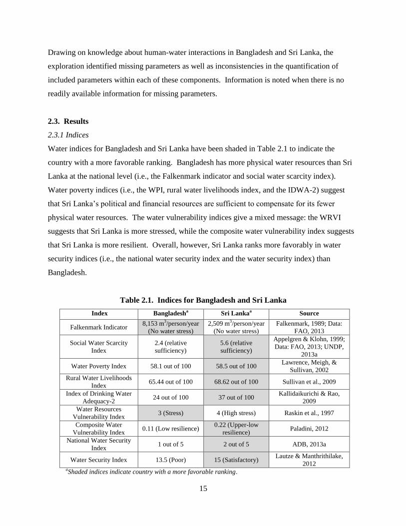
Water indices for Bangladesh and Sri Lanka have been shaded in Table 2.1 to indicate the
country with a more favorable ranking. Bangladesh has more physical water resources than Sri
Lanka at the national level (i.e., the Falkenmark indicator and social water scarcity index).
Water poverty indices (i.e., the WPI, rural water livelihoods index, and the IDWA-2) suggest
that Sri Lanka’s political and financial resources are sufficient to compensate for its fewer
physical water resources. The water vulnerability indices give a mixed message: the WRVI
suggests that Sri Lanka is more stressed, while the composite water vulnerability index suggests
that Sri Lanka is more resilient. Overall, however, Sri Lanka ranks more favorably in water
security indices (i.e., the national water security index and the water security index) than
Bangladesh.
Table 2.1. Indices for Bangladesh and Sri Lanka
Index Bangladesha Sri Lanka
a Source
Falkenmark Indicator 8,153 m
3/person/year
(No water stress)
2,509 m3/person/year
(No water stress)
Falkenmark, 1989; Data:
FAO, 2013
Social Water Scarcity
Index
2.4 (relative
sufficiency)
5.6 (relative
sufficiency)
Appelgren & Klohn, 1999;
Data: FAO, 2013; UNDP,
2013a
Water Poverty Index 58.1 out of 100 58.5 out of 100 Lawrence, Meigh, &
Sullivan, 2002
Rural Water Livelihoods
Index 65.44 out of 100 68.62 out of 100 Sullivan et al., 2009
Index of Drinking Water
Adequacy-2 24 out of 100 37 out of 100
Kallidaikurichi & Rao,
2009
Water Resources
Vulnerability Index 3 (Stress) 4 (High stress) Raskin et al., 1997
Composite Water
Vulnerability Index 0.11 (Low resilience)
0.22 (Upper-low
resilience) Paladini, 2012
National Water Security
Index 1 out of 5 2 out of 5 ADB, 2013a
Water Security Index 13.5 (Poor) 15 (Satisfactory) Lautze & Manthrithilake,
2012 aShaded indices indicate country with a more favorable ranking.
Page 28
16
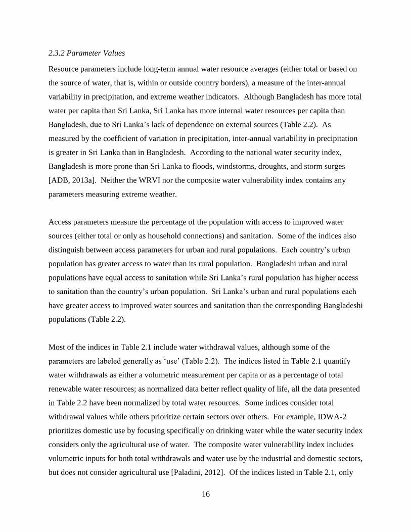
2.3.2 Parameter Values
Resource parameters include long-term annual water resource averages (either total or based on
the source of water, that is, within or outside country borders), a measure of the inter-annual
variability in precipitation, and extreme weather indicators. Although Bangladesh has more total
water per capita than Sri Lanka, Sri Lanka has more internal water resources per capita than
Bangladesh, due to Sri Lanka’s lack of dependence on external sources (Table 2.2). As
measured by the coefficient of variation in precipitation, inter-annual variability in precipitation
is greater in Sri Lanka than in Bangladesh. According to the national water security index,
Bangladesh is more prone than Sri Lanka to floods, windstorms, droughts, and storm surges
[ADB, 2013a]. Neither the WRVI nor the composite water vulnerability index contains any
parameters measuring extreme weather.
Access parameters measure the percentage of the population with access to improved water
sources (either total or only as household connections) and sanitation. Some of the indices also
distinguish between access parameters for urban and rural populations. Each country’s urban
population has greater access to water than its rural population. Bangladeshi urban and rural
populations have equal access to sanitation while Sri Lanka’s rural population has higher access
to sanitation than the country’s urban population. Sri Lanka’s urban and rural populations each
have greater access to improved water sources and sanitation than the corresponding Bangladeshi
populations (Table 2.2).
Most of the indices in Table 2.1 include water withdrawal values, although some of the
parameters are labeled generally as ‘use’ (Table 2.2). The indices listed in Table 2.1 quantify
water withdrawals as either a volumetric measurement per capita or as a percentage of total
renewable water resources; as normalized data better reflect quality of life, all the data presented
in Table 2.2 have been normalized by total water resources. Some indices consider total
withdrawal values while others prioritize certain sectors over others. For example, IDWA-2
prioritizes domestic use by focusing specifically on drinking water while the water security index
considers only the agricultural use of water. The composite water vulnerability index includes
volumetric inputs for both total withdrawals and water use by the industrial and domestic sectors,
but does not consider agricultural use [Paladini, 2012]. Of the indices listed in Table 2.1, only
Page 29
17
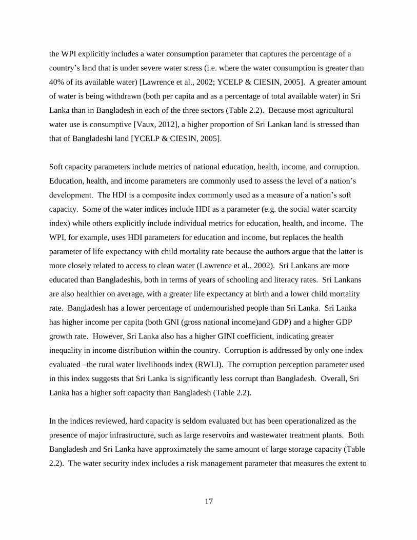
the WPI explicitly includes a water consumption parameter that captures the percentage of a
country’s land that is under severe water stress (i.e. where the water consumption is greater than
40% of its available water) [Lawrence et al., 2002; YCELP & CIESIN, 2005]. A greater amount
of water is being withdrawn (both per capita and as a percentage of total available water) in Sri
Lanka than in Bangladesh in each of the three sectors (Table 2.2). Because most agricultural
water use is consumptive [Vaux, 2012], a higher proportion of Sri Lankan land is stressed than
that of Bangladeshi land [YCELP & CIESIN, 2005].
Soft capacity parameters include metrics of national education, health, income, and corruption.
Education, health, and income parameters are commonly used to assess the level of a nation’s
development. The HDI is a composite index commonly used as a measure of a nation’s soft
capacity. Some of the water indices include HDI as a parameter (e.g. the social water scarcity
index) while others explicitly include individual metrics for education, health, and income. The
WPI, for example, uses HDI parameters for education and income, but replaces the health
parameter of life expectancy with child mortality rate because the authors argue that the latter is
more closely related to access to clean water (Lawrence et al., 2002). Sri Lankans are more
educated than Bangladeshis, both in terms of years of schooling and literacy rates. Sri Lankans
are also healthier on average, with a greater life expectancy at birth and a lower child mortality
rate. Bangladesh has a lower percentage of undernourished people than Sri Lanka. Sri Lanka
has higher income per capita (both GNI (gross national income)and GDP) and a higher GDP
growth rate. However, Sri Lanka also has a higher GINI coefficient, indicating greater
inequality in income distribution within the country. Corruption is addressed by only one index
evaluated –the rural water livelihoods index (RWLI). The corruption perception parameter used
in this index suggests that Sri Lanka is significantly less corrupt than Bangladesh. Overall, Sri
Lanka has a higher soft capacity than Bangladesh (Table 2.2).
In the indices reviewed, hard capacity is seldom evaluated but has been operationalized as the
presence of major infrastructure, such as large reservoirs and wastewater treatment plants. Both
Bangladesh and Sri Lanka have approximately the same amount of large storage capacity (Table
2.2). The water security index includes a risk management parameter that measures the extent to
Page 30
18
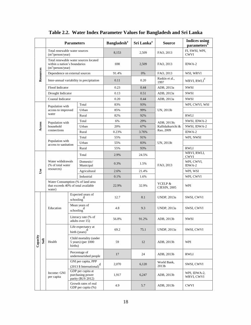
Table 2.2. Water Index Parameter Values for Bangladesh and Sri Lanka
Parameters Bangladesha Sri Lanka
a Source
Indices using
parametersb
Reso
urc
es
Total renewable water sources
(m3/person/year) 8,153 2,509 FAO, 2013
FI, SWSI, WPI,
CWVI
Total renewable water sources located
within a nation’s boundaries
(m3/person/year)
698 2,509 FAO, 2013 IDWA-2
Dependence on external sources 91.4% 0% FAO, 2013 WSI, WRVI
Inter-annual variability in precipitation 0.11 0.20 Raskin et al., 1997 WRVI, RWLI
c
Flood Indicator 0.23 0.44 ADB, 2013a NWSI
Drought Indicator 0.13 0.51 ADB, 2013a NWSI
Coastal Indicator 0.20 0.44 ADB, 2013a NWSI
Access
Population with
access to improved
water
Total 83% 93%
UN, 2013b
WPI, CWVI, WSI
Urban 85% 99%
Rural 82% 92% RWLI
Population with
household
connections
Total 6% 29% ADB, 2013b;
Kallidaikurichi &
Rao, 2009
NWSI, IDWA-2
Urban 20% 67% NWSI, IDWA-2
Rural 0.23% 3.76% IDWA-2
Population with access to sanitation
Total 55% 91%
UN, 2013b
WPI, NWSI
Urban 55% 83%
Rural 55% 93% RWLI
Use
Water withdrawals
(% of total water resources)
Total 2.9% 24.5%
FAO, 2013
WRVI, RWLI,
CWVI
Domestic/ Municipal
0.3% 1.5% WPI, CWVI, IDWA-2
Agricultural 2.6% 21.4% WPI, WSI
Industrial 0.1% 1.6% WPI, CWVI
Water Consumption (% of land area
that exceeds 40% of total available water)
22.9% 32.9% YCELP &
CIESIN, 2005 WPI
Ca
pacit
y
So
ft
Education
Expected years of
schoolingd
12.7 8.1 UNDP, 2013a SWSI, CWVI
Mean years of
schoolingd
4.8 9.3 UNDP, 2013a SWSI, CWVI
Literacy rate (% of
adults over 15) 56.8% 91.2% ADB, 2013b NWSI
Health
Life expectancy at
birth (years)d
69.2 75.1 UNDP, 2013a SWSI, CWVI
Child mortality (under 5 years) (per 1000
births)
59 12 ADB, 2013b WPI
Percentage of undernourished people
17 24 ADB, 2013b RWLI
Income: GNI
per capita
GNI per capita, PPP
(2013 $ International)d
2,070 6,120 World Bank,
2013b SWSI, CWVI
GDP per capita at
purchasing power parity ($US 2012)
1,917 6,247 ADB, 2013b WPI, IDWA-2,
WRVI, CWVI
Growth rates of real
GDP per capita (%) 4.9 5.7 ADB, 2013b CWVI
Page 31
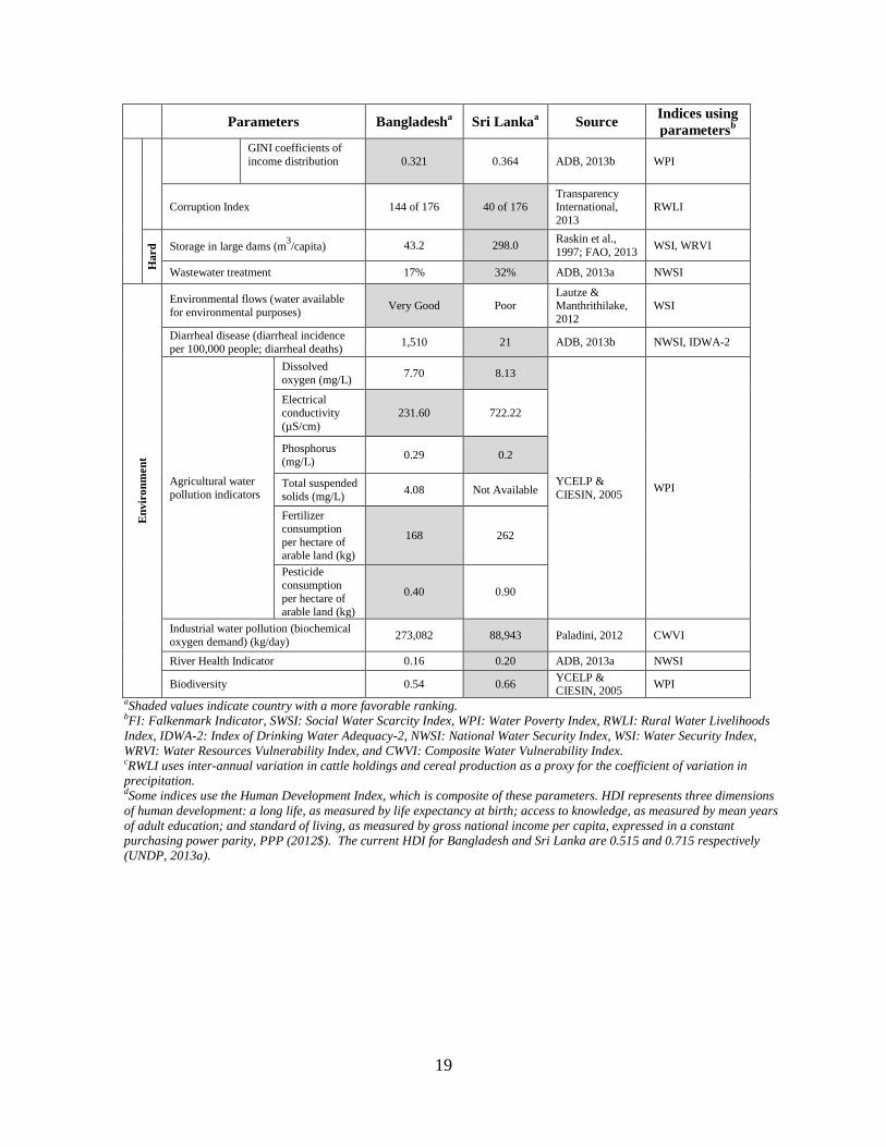
19
Parameters Bangladesha Sri Lanka
a Source
Indices using
parametersb
GINI coefficients of
income distribution
0.321 0.364 ADB, 2013b WPI
Corruption Index 144 of 176 40 of 176 Transparency International,
2013
RWLI
Ha
rd
Storage in large dams (m3/capita) 43.2 298.0
Raskin et al.,
1997; FAO, 2013 WSI, WRVI
Wastewater treatment 17% 32% ADB, 2013a NWSI
En
vir
on
men
t
Environmental flows (water available
for environmental purposes) Very Good Poor
Lautze & Manthrithilake,
2012
WSI
Diarrheal disease (diarrheal incidence
per 100,000 people; diarrheal deaths) 1,510 21 ADB, 2013b NWSI, IDWA-2
Agricultural water
pollution indicators
Dissolved
oxygen (mg/L) 7.70 8.13
YCELP &
CIESIN, 2005 WPI
Electrical conductivity
(µS/cm)
231.60 722.22
Phosphorus
(mg/L) 0.29 0.2
Total suspended
solids (mg/L) 4.08 Not Available
Fertilizer
consumption
per hectare of arable land (kg)
168 262
Pesticide
consumption
per hectare of arable land (kg)
0.40 0.90
Industrial water pollution (biochemical
oxygen demand) (kg/day) 273,082 88,943 Paladini, 2012 CWVI
River Health Indicator 0.16 0.20 ADB, 2013a NWSI
Biodiversity 0.54 0.66 YCELP & CIESIN, 2005
WPI
aShaded values indicate country with a more favorable ranking.
bFI: Falkenmark Indicator, SWSI: Social Water Scarcity Index, WPI: Water Poverty Index, RWLI: Rural Water Livelihoods
Index, IDWA-2: Index of Drinking Water Adequacy-2, NWSI: National Water Security Index, WSI: Water Security Index,
WRVI: Water Resources Vulnerability Index, and CWVI: Composite Water Vulnerability Index. cRWLI uses inter-annual variation in cattle holdings and cereal production as a proxy for the coefficient of variation in
precipitation. dSome indices use the Human Development Index, which is composite of these parameters. HDI represents three dimensions
of human development: a long life, as measured by life expectancy at birth; access to knowledge, as measured by mean years
of adult education; and standard of living, as measured by gross national income per capita, expressed in a constant
purchasing power parity, PPP (2012$). The current HDI for Bangladesh and Sri Lanka are 0.515 and 0.715 respectively
(UNDP, 2013a).
Page 32
20
which countries are buffered from rainfall variability (as measured by the coefficient of variation
of precipitation) through large dam storage (Lautze & Manthrithilake, 2012); nations with higher
inter- and intra-annual variability in rainfall require more infrastructure than nations with little
variability in rainfall. Because Sri Lanka’s higher inter-annual variability is balanced by its
greater upstream storage capacity (Table 2.2), both Bangladesh and Sri Lanka received the same
value for the risk management parameter in the water security index (Lautze & Manthrithilake,
2012). In addition, Sri Lanka currently treats more of its wastewater than Bangladesh (ADB,
2013a).
Ecosystems are extremely complex and are not often addressed in water indices. When
ecosystems are considered, they are often assessed using proxies such as environmental flows
and land cover. The indices reviewed include few consistent parameters that address the
environment. Parameters grouped under the environment component are either water-specific or
general measures of ecosystem health. Environmental flows, or the amount of water unclaimed
for human use and thus available to ecosystems, are greater in Bangladesh than in Sri Lanka
(Table 2.2). Water quality impacts are measured with either human health or chemical pollution
indicators. A common human health indicator is the prevalence of ‘waterborne’ diarrheal
diseases; Bangladesh has more diarrheal incidents per 100,000 people than Sri Lanka (ADB,
2013b). Chemical pollution indicators are either agriculture-specific (i.e. the WPI) or industry-
specific (i.e. the composite water vulnerability index). Sri Lanka consumes more fertilizers and
pesticides per hectare of arable land than does Bangladesh. Biochemical oxygen demand
(BOD), a metric related to dissolved oxygen, reflects the amount of dissolved oxygen needed by
aerobic organisms to break down organic material in water (Penn et al., 2006); Bangladesh has a
much higher industrial BOD than Sri Lanka (Paladini, 2012).
Biodiversity and a composite river health indicator are two general measures of ecosystem health
included in the WPI and the national water security index, respectively. Biodiversity is
measured as the percentage of threatened mammals and birds in the country; biodiversity is
greater in Sri Lanka than in Bangladesh (Lawrence et al., 2002; YCELP & CIESIN, 2005). The
river health indicator values in the national water security index were developed using GIS
(geographic information system) tools to measure pressures and threats to river systems from
Page 33
21
watershed disturbance and pollution activities (such as livestock density), and the vulnerability
of the river systems to alterations in natural flows from infrastructure development and
biological factors (such as river network fragmentation and non-native species) (ADB, 2013a).
Although information regarding soil salinization and non-native species was not provided, the
Asian Development Bank reports that both countries’ rivers are in very poor health, with Sri
Lanka’s rivers being marginally healthier than Bangladesh’s rivers (ADB, 2013a).
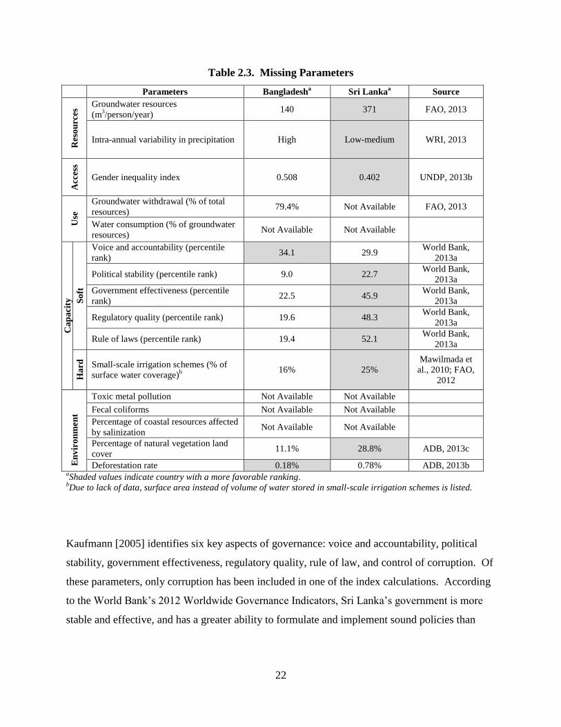
2.3.3 Missing Parameters
During the analysis, numerous missing parameters that could contribute to a comprehensive
understanding of the human-water systems of Bangladesh and Sri Lanka were identified (Table
2.3). Parameters for total, internal, and external water resources are based on long-term annual
averages, which may mask seasonal variations in water availability [Brown & Lall, 2006;
Rijsberman, 2006]. Due to their monsoonal climate, Bangladesh and Sri Lanka both experience
high intra-annual variability in rainfall [Brown & Lall, 2006], which is not accounted for in any
of the indices listed in Table 2.1. Additionally, none of the indices contains any information
regarding the distribution of water resources among surface and groundwater resources. The
distinction between surface and groundwater sources in quantifying water resources is critical
since the two resources have significantly different recharge rates [Hornberger et al., 1998]. Sri
Lanka has more groundwater per capita than Bangladesh [FAO, 2013]. While groundwater
usage information is available for Bangladesh, no such information for Sri Lanka is available
(Table 2.3). Villholth & Rajasooriyar [2010] report that approximately 60% of Sri Lanka’s total
population is currently dependent on groundwater for domestic use.
Although the indices presented in Table 2.1 include valuable access information (such as
distinctions between urban and rural populations), parameters of other intra-group differences are
excluded, notably between men and women. Women have been shown to be disproportionally
affected by lack of water access because they are predominantly responsible for household water
collection, especially in poor households [UNDP, 2006; Sultana, 2007; Sullivan et al., 2009].
Men and women fare more equally in Sri Lanka than in Bangladesh (Table 2.3: gender inequality
index values closer to zero indicate that men and women fare equally).
Page 34
22
Table 2.3. Missing Parameters
Parameters Bangladesha Sri Lanka
a Source
Res
ou
rces
Groundwater resources
(m3/person/year)
140 371 FAO, 2013
Intra-annual variability in precipitation High Low-medium WRI, 2013
Acc
ess
Gender inequality index 0.508 0.402 UNDP, 2013b
Use
Groundwater withdrawal (% of total
resources) 79.4% Not Available FAO, 2013
Water consumption (% of groundwater
resources) Not Available Not Available
Ca
pa
city
So
ft
Voice and accountability (percentile
rank) 34.1 29.9
World Bank,
2013a
Political stability (percentile rank) 9.0 22.7 World Bank,
2013a
Government effectiveness (percentile
rank) 22.5 45.9
World Bank,
2013a
Regulatory quality (percentile rank) 19.6 48.3 World Bank,
2013a
Rule of laws (percentile rank) 19.4 52.1 World Bank,
2013a
Ha
rd
Small-scale irrigation schemes (% of
surface water coverage)b
16% 25%
Mawilmada et
al., 2010; FAO,
2012
En
vir
on
men
t
Toxic metal pollution Not Available Not Available
Fecal coliforms Not Available Not Available
Percentage of coastal resources affected
by salinization Not Available Not Available
Percentage of natural vegetation land
cover 11.1% 28.8% ADB, 2013c
Deforestation rate 0.18% 0.78% ADB, 2013b aShaded values indicate country with a more favorable ranking.
bDue to lack of data, surface area instead of volume of water stored in small-scale irrigation schemes is listed.
Kaufmann [2005] identifies six key aspects of governance: voice and accountability, political
stability, government effectiveness, regulatory quality, rule of law, and control of corruption. Of
these parameters, only corruption has been included in one of the index calculations. According
to the World Bank’s 2012 Worldwide Governance Indicators, Sri Lanka’s government is more
stable and effective, and has a greater ability to formulate and implement sound policies than
Page 35
23
Bangladesh’s government, but the latter’s population ranks higher for voice and accountability
[World Bank, 2013a].
Dams are not the only built infrastructure present in Bangladesh and Sri Lanka. Both reservoirs
and tanks play a large role in stabilizing food production in Sri Lanka (Table 2A.1). Tanks cover
almost 25% of the total surface water storage area in Sri Lanka [Mawilmada et al., 2010].
Similarly, small-scale surface irrigation schemes account for 16% of national irrigation coverage
in Bangladesh [FAO, 2012].
While nutrient pollution is relevant for both countries, none of the indices includes metrics for
water quality issues of significant concern in Bangladesh and Sri Lanka, such as toxic metal
pollution, fecal coliforms, and salinization. Additionally, although deforestation (including the
conversion of forests to agricultural land) continues to threaten Asia, no information on forest
cover or the amount of protected land has been incorporated into any of the indices. Currently, a
higher percentage of Sri Lanka’s land is covered by forests, and more Sri Lankan land is
protected than is Bangladeshi land [ADB, 2013c; WRI,2013]. Annual deforestation rates,
however, are higher in Sri Lanka than in Bangladesh [ADB, 2013b].
2.4 Discussion
While water indices can facilitate program evaluation and serve as tools for water managers, as
stated in Section 2.1, the findings from water indices can be ambiguous. Unlike parameter level
comparisons, index level comparisons offer limited insight on small geographic scales. Our
parameter level analysis has shown specific metrics (e.g. education and income) that contribute
to Sri Lanka’s improved indices. Water index parameters, however, have limitations as outlined
below.
The most notable issue uncovered during the analysis was the absence of key parameters that
could greatly impact overall water indices (Table 2.3). While no single index can capture all of
the complex interactions implicit in human-water systems, the omission or inclusion of key
parameters can alter the conclusions drawn from an index [Grey & Sadoff, 2007]. For example,
parts of both Bangladesh’s and Sri Lanka’s populations rely predominantly on groundwater
Page 36
24
resources, which has resulted in aquifer depletion in both countries [Senaratne, 1996; Shah et al.,
2003; Brown & Lall, 2006; ADB, 2013a]. Furthermore, declining groundwater levels in
Bangladesh are affecting water quality, causing adverse effects on soils, and limiting crop
growth [FAO, 2012]. However, groundwater resource or usage data for both countries are
glaringly absent from all the evaluated indices. This absence is in part due to a lack of available
information, so policy makers and water managers should ensure that groundwater resource and
usage data are being collected to help develop a comprehensive understanding of the current
state of their water resources.
Similarly absent from the indices is water-specific information regarding capacity and water
quality parameters. It should be noted that while general governance information is valuable, it
gives little insight into the specific structure and management of water infrastructure. The
general World Bank Governance Indicator for government effectiveness, for example, does not
seem to adequately represent the concerns arising from limited coordination between Sri Lanka’s
water agencies. Education metrics (e.g. literacy rate) also provide little information regarding
awareness of basic hydrological concepts such as the water cycle and how to limit contamination
of water supplies. Future research should assess how information on water-specific governance
and education can be collected and measured. While not a comprehensive list, Table 2.3 lists
additional parameters that should be evaluated for inclusion in water indices. Until these data
become available, the rationale for using certain proxies should be explicitly stated in analyses.
Few of the evaluated indices consider the complex relationships between the components. The
water security index is one of the few indices to include a risk management parameter to measure
the extent to which a nation is buffered from rainfall variability through large dam storage.
Similarly, the presence of water agreements with neighboring countries suggests that a country’s
external water resources should not be ignored. Most of the evaluated indices, however, give
equal weight to the parameters listed in Table 2.2, rather than examining these complex
relationships when developing indices. Since the indices typically have more parameters
reflecting social conditions than physical conditions, Sri Lanka has more favorable water indices
despite having a third of Bangladesh’s total water resources available per capita (Tables 2.1 and
2.2). Equal weighting of all parameters also causes valuable information to be lost. For
Page 37
25
example, in addition to having greater income per capita, Sri Lanka also has higher income
inequality (as indicated by the GINI coefficient and the percentage of undernourished people)
than Bangladesh.
The indices evaluated did not always reflect the framework implied in their nomenclature. For
example, the WRVI has no parameters measuring natural hazards but the national water security
index does. In addition, the WPI includes parameters measuring agricultural water quality,
which are not present in any of the other indices. Inconsistencies in parameter units are also
present. For example, some of the indices use only per capita volumetric measurements,
whereas the percentage of water used relative to total water resources is a better indicator of the
stress on a nation’s water resources. Some indices also have issues with double counting: the
composite water vulnerability index, for example, has a parameter representing total water use as
well as additional parameters for water use by the industrial and domestic sectors [Paladini,
2012].
2.5 Conclusion
This analysis demonstrates that policy makers, water managers, and academics should use water
indices with caution. Human-water systems are extremely complex, and not all of their
parameters can been compassed by any one index. Therefore, researchers and water managers
should be cautious when selecting and applying an index to monitor progress towards their
national goals. Particular attention should be given to the selection of parameters relevant to
national priorities. When possible, parameters that reflect complex hydrological characteristics
and contain water-specific metrics should be used. Regardless of the shortcomings outlined
here, water indices are a valuable method to integrate physical and social factors influencing
human-water systems. Following these recommendations will improve the likelihood of these
indices providing a comprehensive representation of the most critical aspects of a nation’s water
resource issues.
2.6 Acknowledgements
This material is based upon work supported by the Office of Naval Research through Grant No.
Page 38
26
N00014-11-1-0683 and the National Science Foundation Graduate Research Fellowship Program
under Grant No. DGE-0909667 and by WSC program Grant No. NSF-EAR 1204685. We would
like to thank George Hornberger and Jonathan Gilligan for their feedback.
2.7 References
Appelgren, B. & W. Klohn, 1999. Management of water scarcity: a focus on social capacities
and options. Physics and Chemistry of the Earth, Part B: Hydrology, Oceans and Atmosphere
24(4), 361–373.
Asian Development Bank (ADB), 2013a. Asian water development outlook 2013: measuring
water security in Asia and the Pacific. Asian Development Bank, Mandaluyong City,
Philippines.
Asian Development Bank (ADB), 2013b. Key development indicators for Asia and the Pacific,
Manila, Philippines. Available at: http://www.adb.org/ publications/series/key-indicators-for-
asia-and-the-pacific (Accessed August 23 2013).
Asian Development Bank (ADB), 2013c. Economic and research development: basic statistics
2013 spreadsheet. Available at: http://www.adb.org/publications/basic-statistics-2013 (Accessed
August 23 2013).
Biswas, A. K. & K. E. Seetharam, 2008. Achieving water security for Asia. International
Journal of Water Resources Development 24, 145–176.
Brown, A. & M. D. Matlock, 2011. A review of water scarcity indices and methodologies. Food,
Beverage, and Agriculture:White Paper #106.
Brown, C. & U. Lall, 2006. Water and economic development: the role of variability and a
framework for resilience. Natural Resources Forum 30(4), 306–317.
Chenoweth, J., 2008. A re-assessment of indicators of national scarcity. Water International
33(1), 5–18.
Cook, C. & K. Bakker, 2012. Water security: debating an emerging paradigm. Global
Environmental Change 22, 94–102.
Falkenmark, M., 1989. The massive water scarcity threatening Africa – why isn’t it being
addressed? Ambio 18(2), 112–118.
Food and Agricultural Organization (FAO), 2007. Coping with water scarcity: challenge of the
twenty-first century. Available at: http://www.fao.org/nr/water/docs/escarcity.pdf (Accessed
May 21 2014).
Page 39
27
Food and Agricultural Organization (FAO), 2012. Irrigation in southern and eastern Asia in
figures, AQUASTAT Survey – 2011. FAO Water Report #37. Available at:
http://www.fao.org/docrep/016/i2809e/i2809e.pdf (Accessed August 1 2013).
Food and Agricultural Organization (FAO), 2013. AQUASTAT database. Available at:
http://www.fao.org/nr/water/aquastat/main/index.stm (Accessed May 1, 2013).
Feitelson, E. & J. Chenoweth, 2002. Water poverty: towards a meaningful indicator. Water
Policy 4(3), 263–281.
Gain, A. K., C. Giupponi and F.G. Renaud, 2012. Climate change adaptation and vulnerability
assessment of water resources systems in developing countries: a generalized framework and a
feasibility study in Bangladesh. Water 4(4), 345–366.
Gleick, P. H. ,2003. Global freshwater resources: soft-path solutions for the 21st century.
Science 302(5650), 1524–1528.
Grey, D. & C.W. Sadoff, 2007. Sink or swim? Water security for growth and development.
Water Policy 9, 545–571.
Hornberger, G. M., J. P. Raffensperger, P. L. Wiberg and K. N. Eshleman, 1998. Elements of
Physical Hydrology. Johns Hopkins University Press, Baltimore, MD.
Kallidaikurichi, S. & B. Rao, 2009. Index of drinking water adequacy for the Asian economies.
Institute of Water Policy, Working Paper No.2/2009.
Kaufmann, D., 2005. Myths and realities of governance and corruption. Available at:
http://mpra.ub.uni-muenchen.de/8089/1/Myths_Realities_Gov_Corruption.pdf (Accessed July 1
2010).
Kelly, P. M. & W. N. Adger, 2000. Theory and practice in assessing vulnerability to climate
change and facilitating adaptation. Climatic Change 47, 325–352.
Lautze, J. & H. Manthrithilake, 2012. Water security: old concepts, new package, what value?
Natural Resources Forum 36: 76–87.
Lawrence, P., J. Meigh and C. Sullivan, 2002. The water poverty index: an international
comparison. Keele economics research papers, 2002/19. Available at:
http://128.118.178.162/eps/dev/papers/0211/0211003.pdf (Accessed October 21 2014).
Mawilmada, N., S. Atapattu, J. Dela, N. Gunawardene, B. Weerasinghe, M. Nandana, A.
Bellanwawithana, R Wimalasiri and N. Kumari, 2010. Sector vulnerability profile: Sri Lanka.
supplementary document to: the national climate change adaptation strategy for Sri Lanka 2011
to 2016. Available at: http://www.climatechange.lk/adaptation/Files/Water_
SVP_Nov-16-2010.pdf (Accessed July 29 2013).
Page 40
28
Molden, D., 2007. Water for food, water for life: a comprehensive assessment of water
management in agriculture (ed.) Earthscan, London, UK and International Water Management
Institute, Colombo, Sri Lanka.
Molle, F. & P. Mollinga , 2003. Water poverty indicators: conceptual problems and policy
issues. Water Policy 5(5), 529–544.
Paladini, S. 2012. Evaluating Water security in the Asia-Pacific region: a new approach based
on vulnerability indices. Eurasian Geography and Economics 53(1), 95–114.
Penn, M. R., J.J. Pauer and J.R. Mihelcic, 2006. ‘ Biochemical oxygen demand’. IN:
Environmental and Ecological Chemistry. A. Sabljic (ed.). Vol. 2, EOLSS.
Plummer, R., R. Loë & D. Armitage, 2012. A systematic review of water vulnerability
assessment tools. Water Resources Management 26(15), 4327–4346.
Raskin, P., P. Gleick, P. Kirshen, G. Pontius and K. Strzepek, 1997. Water futures: assessment
of long-range patterns and prospects. Stockholm Environment Institute, Stockholm, Sweden.
Rijsberman, F. R., 2006. Water scarcity: fact or fiction? Agricultural Water Management 80, 5–
22.
Seckler, D., U. Amrasinghe, D. Molden, R. de Silva and R. Barker, 1998. World water demand
and supply, 1990 to 2025: scenarios and issues. Research Report #19, International Water
Management Institute, Colombo, Sri Lanka.
Senaratne, A., 1996. Use of groundwater to alleviate water deficit during dry season (Yala) in
the NCP of Sri Lanka . A report submitted to the Sri Lanka national Program office of the IIMI,
Battarmulla, Sri Lanka.
Shah, T., A. D. Roy, A. S. Qureshi and J. Wang, 2003. Sustaining Asia’s groundwater boom: an
overview of issues and evidence. Natural Resources Forum 27(2), 130–141.
Sullivan, C. 2002. Calculating a water poverty index. World Development 30(7), 1195–1210.
Sullivan, C. A., A. Cohen, J. M. Faurès and G. Santini, 2009. The rural water livelihoods index.
Working paper, Food and Agricultural Organization of the United Nations, Rome. Available at:
http://www.fao.org/nr/water/docs/FAOW_RWLI_paper.pdf (Accessed May 5 2013).
Sullivan, C. & J. Meigh, 2003. Considering the water poverty index in the context of poverty
alleviation. Water Policy 5, 513–528.
Sullivan, C. A., J. R Meigh, T. Giacomello, T. Fediw, P. Lawrence and M. Samad, 2003. The
water poverty index: development and application at the community scale. Natural Resources
Forum 27, 189–199.
Page 41
29
Sultana, F., 2007. Water, water everywhere, but not a drop to drink: pani politics (water politics)
in rural Bangladesh. International Feminist Journal of Politics 9(4), 494–502.
Transparency International, 2013. 2012 Corruptions perceptions index. Available at:
http://cpi.transparency.org/cpi2012/ (Accessed May 20 2013).
United Nations (UN), 2013a. International decade for action ‘water for life’ 2005–2015.
Available at: http://www.un.org/ waterforlifedecade/scarcity.shtml (Accessed August 10 2013).
United Nations (UN), 2013b. Millennium development goals indicators database. Available at:
http://millenniumindicators.un.org/unsd/mdg/Data.aspx (Accessed August 1 2013).
United Nations Development Programme (UNDP), 2006. Human development report 2006:
beyond scarcity: power, poverty and the global water crisis. Available at:
http://hdr.undp.org/sites/default/files/reports/267/hdr06-complete.pdf (Accessed October 21
2014).
United Nations Development Programme (UNDP), 2013a. Human development report 2013:
The rise of the South: human progress in a diverse world. Available at:
http://hdr.undp.org/en/reports/global/hdr2013/ (Accessed August 2 2013).
United Nations Development Programme (UNDP), 2013b. Gender inequality index. Available
at: http://hdr.undp.org/en/statistics/gii/ (Accessed August 2 2013).
UN-Water, 2013. Water security & the global water agenda: a UN-water analytical brief.
Vaux, H., 2012. Water for agriculture and the environment: the ultimate trade-off. Water Policy
14(S1): 136.
Villholth, K. G. & L. D. Rajasooriyar, 2010. Groundwater resources and management
challenges in Sri Lanka – an overview. Water Resources Management 24(8), 1489–1513.
World Bank, 2013a. Governance indicators. Available at:http://info.worldbank.org/governance
/wgi/mc_chart.asp (Accessed August 10 2013).
World Bank, 2013b. Gross national income. Available at: http://data.worldbank.org/indicator/
NY.GNP.PCAP.PP.CD(Accessed September 4 2013).
World Health Organization (WHO) & UNICEF, 2012. Progress on drinking water and
sanitation. Joint MonitoringProgramme update 2012. Available at:
http://www.who.int/water_sanitation_health/publications/2012/jmp_report/en/index.
html (Accessed December 1 2013).
World Resources Institute (WRI), 2013. Aqueduct water risk atlas. Available at:
http://aqueduct.wri.org/atlas (Accessed July15 2013).
Page 42
30
Yale Center for Environmental Law and Policy (YCELP) & Center for International Earth
Science Information Network (CIESIN) of Columbia University, 2005. 2005 Environmental
sustainability index: benchmarking national environmental stewardship.
Appendix: Country Descriptions
Bangladesh
Bangladesh, a least developed country, is one of the most densely populated countries in the
world [UNCTAD, 2011; FAO, 2012]. Bangladesh is a riverine country with 7% of
the country’s total land area covered by rivers, notably the Ganges, Brahmaputra, and Meghna
[FAO, 2012]. More than 90% of Bangladesh’s surface water originates in other countries
[Chowdhury, 2010]. The majority of rain falls during the annual monsoon, from June to
Table 2A.1 Bangladesh and Sri Lanka Country Profiles
Bangladesh Sri Lanka Source
Land area (km2) 144,000 25,332 FAO, 2012
Population (x1000) 150,494 21,025 FAO, 2013
Population density
(inhabitants/km2) 1,045 321 FAO, 2013
Population growth rate (%) 1.3 0.7 ADB, 2013b
Mean annual temperature (°C) 25°C
27°C in the lowlands,
15°C in the central
highlands FAO, 2012
Total cultivable land area (hectares
per capita) 0.06 0.10 FAO, 2013
Gross domestic product, PPP ($US
2012 per capita) 1,943 6,040 ADB, 2013b
September, when 80% of the annual precipitation occurs [Chowdhury, 2010]. The country
receives an annual average of 2,320 millimeters (mm) of rain but there is significant spatial
variation in the amount of rainfall received, with an annual average of 1,110 mm of rainfall in
the west and over 5,000 mm in the north-east [FAO, 2012; 2013]. Water is the primary
transportation medium, and water-intensive industries such as agriculture, fisheries, forestry, and
aquaculture are significant contributors to Bangladesh’s economy.
Page 43
31
Currently, groundwater is the primary water source in Bangladesh, comprising 79% of total
water use in 2008 [FAO, 2012]. The agricultural sector, particularly paddy cultivation, is the
biggest water user, accounting for 88% of the country’s total water withdrawals in 2008
[Chowdhury, 2010; FAO, 2013].
Bangladesh is extremely vulnerable to frequent floods, cyclones, droughts, and storm surges.
Due to its flat and low-lying topography, sea level rise is also of concern [Chowdhury, 2010].
Although the country has plentiful water during the monsoon season, there is insufficient storage
throughout the country to meet the needs of people and agriculture during the dry season [FAO,
2012]. Furthermore, water quality has been adversely impacted by agricultural run-off, fecal
contamination due to inadequate sanitation, saltwater intrusion, and pollution from industrial
sources. To address contamination of surface water, in the 1970s, the Bangladesh government
initiated a nationwide program to provide shallow groundwater tube wells to many rural
residents. This provided a dependable alternative drinking water supply until arsenic
contamination was discovered in 1994 [Biswas & Adank, 2004]. Today, an estimated 1 million
tube wells are contaminated with arsenic, exposing over 30 million people to its toxic effects
[Chowdhury, 2010; FAO, 2013]. Increased salinity in surface water has occurred because of
decreased flows, and saltwater intrusion in the coastal areas is evident in groundwater drinking
wells [Chowdhury, 2010; FAO, 2013].
The Ministry of Water Resources (MoWR) is responsible for the planning, implementation and
operation of all water resource activities in Bangladesh. Two of the major institutions under
MoWR are the Bangladesh Water Development Board (BWDB) and the Water Resources
Planning Organization (WARPO). WARPO has national and regional water planning
responsibilities, and the BWDB is charged with the execution of over 400 water projects. The
National Water Resources Council (NWRC) is the national body responsible for water policy in
Bangladesh. WARPO has a mandate to coordinate with all relevant ministries through the
NWRC [Chowdhury, 2010]. Delivery of water and sewerage services in the larger cities is the
responsibility of the water and sanitation authorities, whereas local governments implement
water supply projects in the smaller municipalities. The Department of Public Health
Engineering (DPHE) is the national agency responsible for water and sanitation facilities in the
Page 44
32
rural areas [Chowdhury, 2010]. Non-governmental organizations are primarily responsible for
implementing or extending water services in the country, either directly or indirectly through
micro-finance assistance [Biswas & Adank, 2004]. Bangladesh reached an agreement with India
regarding equitable use of the Ganges in 1996, but no such agreements have been made for the
other trans-border rivers [FAO, 2012]. Water rights in the country are linked to land ownership
rights, but over 45% of the rural population in the country is either landless or ‘functionally
landless’, owning less than 200 square meters of land [World Bank, 2013].
Sri Lanka
Sri Lanka, an island nation, is divided into three climatic zones determined by rainfall patterns:
the wet zone, the intermediate zone, and the dry zone. Sri Lanka receives rain from two
monsoons, the north-east monsoon and the south-west monsoon. The wet zone receives rain
during both the north-east and south-west monsoon, while the dry zone, which covers three-
quarters of the island, receives rain only during the north-east monsoon.
As in Bangladesh, there is high spatial variation in the rainfall patterns, with an average annual
rainfall of less than 1,000 mm in the north-west and over 5,000 mm in the central highlands of
the country [Gunatilaka, 2008]. Both floods and drought are issues of particular concern in parts
of the island [FAO, 2012]. Because Sri Lanka is an island nation, it has no trans-border water
resources. Water quality issues include agricultural pollution, fecal contamination, and saltwater
intrusion, notably in the coastal areas [Villholth & Rajasooriyar, 2010].
As in Bangladesh, agriculture (predominantly paddy cultivation) plays a large role in the local
Sri Lankan economy. In Sri Lanka, irrigation schemes are classified as minor, medium, and
major depending on the size of the area that can be irrigated by the scheme. Small artificial lakes
and ponds, known locally as tanks, dominate the minor irrigation systems [Marambe et al.,
2012]. Due to overcrowding in other parts of the country, the Sri Lankan government initiated
the Mahaweli Development Programme in the 1970s, which oversees the construction of
medium and major irrigation systems in the dry zone.
Page 45
33
There are approximately 40 institutions and 40 legislative acts related to water in Sri Lanka
[Manthrithilake& Liyanagama, 2012]. Small-scale irrigation schemes are under the purview of
the Department of Agrarian Development and are primarily managed by the farmers themselves.
Medium and large irrigation schemes in the dry zone are managed collaboratively by the
Mahaweli Authority of Sri Lanka and the Irrigation Department with priorities given to drinking
and irrigation water over electricity generation [Manthrithilake & Liyanagama, 2012]. Unlike
the set-up in Bangladesh, there is little coordination in managing general water resources in the
country; for example, the Meteorological Department and the Irrigation Department both collect
rainfall data but neither shares their data with the other agency [FAO, 2012; Thuraisingham,
2013]. Overlap, gaps, and conflicting jurisdictions arise from Sri Lankan water laws being
administered at the agency level rather than being coordinated under a single ministry [FAO,
2012]. Water rights in Sri Lanka are linked to land ownership, so landowners have full authority
over the use of surface water and groundwater resources accessible on their land [FAO, 2012].
Nevertheless, land fragmentation, landlessness, and encroachment in Sri Lanka generate
inequality in access to water rights [Azmi, 2007]. To date, no comprehensive groundwater
management or planning systems have been implemented in the country [FAO, 2012].
Appendix References
Asian Development Bank (ADB), 2013b. Key development indicators for Asia and the Pacific,
Manila, Philippines. Available at: http://www.adb.org/publications/series/key-indicators-for-asia-
and-the-pacific (Accessed August 23 2013).
Azmi, F., 2007. Changing livelihoods among the second and third generations of settlers in
system H of the accelerated Mahaweli Development Project (AMDP) in Sri Lanka. Norsk
Geografisk Tidsskrift – Norwegian Journal of Geography 61(1), 1–12.
Biswas, S. & M. Adank, 2004. Cost recovery and financing of rural water supply in bangladesh:
a case study. Natural Resource Centre, NGO Forum for Drinking Water Supply and Sanitation.
Available at: http://www.irc.nl/content/download/
22110/258575/file/cost_recovery_and_financing.pdf (Accessed May 21 2014).
Chowdhury, N. T., 2010. Water management in Bangladesh: an analytical review. Water
Policy, 12(1020), 32–51.
Food & Agriculture Organization (FAO) of the United Nations, 2012. Irrigation in Southern and
Eastern Asia in figures, AQUASTAT Survey – 2011. FAO Water Report #37. Available at:
http://www.fao.org/docrep/016/i2809e/i2809e.pdf (Accessed August 1 2013).
Page 46
34
Food & Agriculture Organization (FAO) of the United Nations, 2013. AQUASTAT Database.
Available at: http://www.fao.org/nr/water/aquastat/main/index.stm (Accessed May 1,2013).
Gunatilaka, A., 2008. Water security and related issues in Sri Lanka: the need for integrated
water resource management (IWRM). Journal of the National Science Foundation of Sri Lanka
36(Special), 3–15.
Manthrithilake, H. & B. S. Liyanagama, 2012. Simulation model for participatory decision
making: water allocation policy implementation in Sri Lanka. Water International 37(4), 478–
491.
Marambe, B., G. Pushpakumara, and P. Silva, 2012. Biodiversity and agrobiodiversity in Sri
Lanka: village tank systems. IN: the biodiversity observation network in the Asia-pacific region:
toward further development of monitoring, ecological research monographs, Tokyo, Springer
Japan.
Thuraisingham, M., 2013. Interview with Mr. M. Thuraisingham, Additional Director General
of Irrigation on 4 June 2013.
United National Conference on Trade and Development (UNCTAD), 2011. The Least
developed countries in 2011: the potential role of south-south cooperation for inclusive and
sustainable development. Available at: http://unctad.org/en/Docs/ldc2011_en.pdf (Accessed
August 20 2013).
Villholth, K. G. & L. D. Rajasooriyar, 2010. Groundwater resources and management
challenges in Sri Lanka – an overview. Water Resources Management 24(8), 1489–1513.
World Bank, 2013. Bangladesh: Priorities for Agriculture and Rural Development. Available
at:http://web.worldbank.org/wbsite/external/countries/southasiaext/extsaregtopagri/0,contentmdk
:20273763~menupk:548213~pagepk: 34004173~pipk:34003707~thesitepk:452766,00.html
(Accessed August 22 2013).
Page 47
35
CHAPTER 3
Drinking Water Insecurity: Water Quality and Access
in Coastal South-Western Bangladesh
This chapter was published in the International Journal of Environmental Health Research,
ISSN: 0960-3123 (print), 1369-1619 (online) June 8, 2016.
ABSTRACT
National drinking water assessments for Bangladesh do not reflect local variability, or temporal
differences. This paper reports on the findings of an interdisciplinary investigation of drinking
water insecurity in a rural coastal south-western Bangladesh. Drinking water quality is assessed
by comparison of locally measured concentrations to national levels and water quality criteria;
resident’s access to potable water and their perceptions are based on local social surveys.
Residents in the study area use groundwater far less than the national average; salinity and local
rainwater scarcity necessitates the use of multiple water sources throughout the year.
Groundwater concentrations of arsenic and SpC were greater than surface water (pond)
concentrations; there was no statistically significant seasonal difference in mean concentrations
in groundwater, but there was for ponds, with arsenic higher in the dry season. Average arsenic
concentrations in local water drinking were 2 to 4 times times the national average. All of the
local groundwater samples exceeded the Bangladesh guidance for SpC, although the majority of
residents surveyed did not perceive their water as having a "bad" or "salty" taste.
3.1 Introduction
Water is essential to life and human health, economic development, food security, poverty
reduction, and sustainable ecological functions [UN Water, 2013]. Given that the world’s
population is expected to reach eight billion by 2025, growing demands on drinking water
supplies and water for food production are evident, and competing uses of limited resources are
inevitable [UNDP, 2006]. Anticipated anthropogenic climate change impacts of higher
temperatures, drought, more erratic precipitation patterns, and more intense storms are expected
to intensify water demands [IPCC, 2007]. There are myriad terms that describe human social
and environmental relationships with water. One of the most comprehensive terms currently
being used is “water security”, which UN Water defines as:
The capacity of a population to safeguard sustainable access to adequate quantities of
acceptable quality water for sustaining livelihoods, human well-being, and socio-
economic development, for ensuring protection against water-borne pollution and water-
related disasters, and for preserving ecosystems in a climate of peace and political
stability. [UN Water, 2013, p.1].
Page 48
36
Many drinking water assessments for Bangladesh have focused at the national level that does not
reflect local variability, nor illustrates temporal differences due to the seasonality of water
supplies. The objective of this paper is to report on the findings of an interdisciplinary
investigation of the state of drinking water security in a small area of coastal south-western
Bangladesh to illustrate the importance of scale in assessing water security. The assessment of
local water security is focused on water quality and the issues that affect access to potable water.
The types of local water sources and uses are described, and spatial and temporal trends in local
water quality are identified. Drinking water quality is assessed by comparison of locally
measured concentrations to national concentrations and to water quality criteria, and resident’s
access to potable water are described based on local social surveys.
3.1.1 Factors affecting water security in Bangladesh
The coastal region of Bangladesh is predominantly rural, relying on rice paddy farming, fishing,
and aquaculture for its primary livelihoods [Chowdhury, 2010; FAO, 2009]. Shrimp farming has
intensified over the past two decades, greatly changing the local landscape, and negatively
affecting surface and groundwater resources [Datta et al., 2010].
Throughout Bangladesh ineffective water management, insufficient governance, and the lack of
infrastructure greatly affects water security, and drinking water needs compete with irrigation
demands. Agriculture employs about two-thirds of the country’s population, and rice cultivation
is the most important activity, requiring vast amounts of surface water and groundwater for
irrigation [Chowdhury, 2010; Abedin et al., 2014]. Food security for the nation is thus heavily
water-dependent [Falkenmark, et al. 2009; UNESCO, 2012].
Drinking water sources in rural are varied, and include shallow groundwater obtained through
tubewells, small ponds with and without pond sand filters (PSF, a sand and gravel filter),
harvested rainwater, bottled water, and river water. Rainwater collection devices are of generally
small volume (insufficient to last the entire year), and municipal reservoirs are essentially non-
existent. This lack of adequate water storage infrastructure intensifies water insecurity [Ansari et
al., 2011].
Page 49
37
Bangladesh is vulnerable to water insecurity partially because of its environmental
circumstances. Being a low-lying deltaic country of exceptionally dense population, Bangladesh
is susceptible to a variety of environmental stresses and natural disasters; these stresses can
exacerbate the difficulties accessing potable water [FAO, 2009; Chowdhury, 2010; Abedin, et al.
2014]. For example, south-west Bangladesh was severely impacted by cyclone Aila in 2009;
many drinking water sources were inundated with saline tidal water and became unusable [FAO,
2009; Mallick, et al. 2011].
Although the country has immense natural water resources, drinking water quantity and quality
are greatly affected by Bangladesh's monsoonal climate. Rainfall in Bangladesh is not consistent
temporally or spatially; 80% of the rainfall occurs during June to September [Chowdhury, 2010;
Abedin et al., 2014]. This seasonal nature of water supply affects the choices people make in
selecting drinking sources and the quality of those sources. The long dry season results in local
water scarcity and degraded water quality, and necessitates the use of multiple drinking water
sources to meet basic personal needs [Ansari et al., 2011]. In the dry season, rainwater is not
available for drinking, and surface water sources become stagnant.
Groundwater is used extensively for drinking water throughout Bangladesh. On the coast, most
of the groundwater used for water supply is pumped from the top 150 meters, but much of it is
saline [Chowdhury, 2010; Ravenscroft, 2003]. Aquifers would be expected to be flushed and
recharged seasonally during the monsoon, bringing an abundance of fresh subsurface water, but
recharge is highly variable due to the presence of intermittent, thick deposits of clays
[Ravenscroft, 2003]. Over one million community tubewells and 10 million private tubewells
are in use in Bangladesh [BBS, 2012]. It has been estimated that 15 to 100 people are served by
one tube well [WASSA, 2004; BBS, 2011].
In Bangladesh, the main issues surrounding water quality are microbial pathogens, arsenic (As)
in groundwater, and salinity. Although a significant issue, bacterial contamination of water is
not addressed here. For decades, the widespread contamination of groundwater by As in
Bangladesh has been recognized as a severe problem [Ahmed et al., 2006; Ahmed, 2011].
Page 50
38
Although it is naturally-occurring, As contamination is a continuing public health issue in
Bangladesh, potentially affecting millions of people [Chowdhury, 2010; BBS, 2011]. Salinity
has been recognized as a significant water problem in coastal Bangladesh for some time, as a
result of both man-made and natural causes [Uddin, 2003; Rahman & Bhattacharya, 2006;
Mahmuduzzaman et al., 2014]. While water quality in Bangladesh has been acknowledged as a
problem, many studies focus on either arsenic or salinity, not both. What has not readily been
recognized, however, is drinking water that contains arsenic also contains numerous other toxic
chemicals, so the risk to residents is vastly under reported because risks are considered
cumulative [USEPA, 2007; WHO, 2011].
3.1.2 Impacts of water insecurity
The effects on human health from poor water quality are well-known [WHO & UNICEF, 2011].
Chronic exposure to high levels of arsenic is associated with a multitude of health issues
including cancers, cardiovascular disease, and skin lesions [Joseph et al., 2015]. The health
effects of dietary salt intakes are understood and well-documented. However, studies on health
effects of drinking saline water are scarce. Khan et al. [2011; 2014] demonstrated significant
risk of pre/eclampsia and gestational hypertension in women in the Dacope upazila of
Bangladesh; rates were higher in coastal residents compared to non-coastal areas. Khan also
showed that women consuming tubewell drinking water were at higher health risks than those
who used pond water or rainwater [Khan et al., 2014]. Health impacts were also found to be
considerably higher in the dry season than in the monsoon season [Khan, 2008].
Not only are there adverse health effects to people from drinking contaminated water, but there
are lost opportunity costs associated with the time in collecting water, and time spent away from
education and occupational pursuits; all of these are considered to affect both an individual’s and
a community’s development potential [UNDP, 2006]. In Bangladesh, as in many developing
countries, women carry the burden of water collection. Internationally, it has been estimated that
64% of water collection duties fall to women [WHO & UNICEF, 2011].
Page 51
39
3.1.3 Assessment of water security on a national basis
Bangladesh was issued a Millennium Development Goal [MDG] in 2000 to halve the proportion
of people in the country that do not have access to safe drinking water by 2015 [UN, 2000].
There was no specific quality requirement; water was considered “safe” if obtained from an
“improved water source” [tubewells are considered “improved”, but ponds are not] [WHO &
UNICEF, 2000; 2011]. Taking arsenic contamination of groundwater into consideration, it was
estimated in 2015 that 86% of Bangladesh’s population is considered to have access to safe
drinking water, well towards its goal of 89% [GOB, 2015; BBS, 2011]. However, this method of
estimating access to "safe" water is flawed because it does not address the quality of drinking
water; access issues such as seasonal availability, the number of sources used, and time it takes
to collect water; or the reliability of the sources.
In Bangladesh, the population that continues to be without safe water is the country’s poorest and
most vulnerable. Support documentation for the MDG defines distance to an “improved source”
as within one kilometre (1 km) of the dwelling. Although the MDG does not account for the
time needed to collect water, for accounting purposes, the time taken for water collection is
usually assumed to be 30 minutes or less, round trip [UNESCO, 2009]. The success of a rural
water supply is directly related to the ability to keep it in working order, which is related to who
owns the source, where it is located, its acceptance by the community, and local leadership
[Crow & Sultana, 2002; WHO & UNICEF, 2011].
All of the factors described that contribute to water security at the national level also affect water
security at the local level. The complexity and variability of these factors suggest that water
security assessed at a national level could miss significant differences, and might be better
assessed at the local scale, as described in this study.
3.1.4 Study Area
The study area is “Polder 32” (P32), located in the Khulna district, Dacope upazila in southwest
Bangladesh, 60 km north of the Bay of Bengal. The upazila is located between 22°24' N and
22°40' N and 89°24' E and 89°35' E. This area was devastated by cyclone Aila in 2009 [Mehedi,
2010], and at the time of this study (2012), parts of the polder were still recovering. Dacope
Page 52
40
upazila has 10 unions and 716 mauzas (which are basically comparable to census blocks in the
US). P32 consists of two unions: one north (Kamarkhola), which consists of two mauzas:
Kamarkhola and Sreenagar/Kalinagar, and one south (Sutarkhali), which consists of four
mauzas: Sutarkhali, Gunari, Nalian, Kalibogi/ Sutarkhali [BBS, 2012]. P32 is home to
approximately 44,000 people is about 19 km long and 7 km wide (Table 3.1).
Table 3.1. National and Local Demographics (2011 Census)a
aSources: [BBS, 2012; 2014; 2015]; na=not available.
bPolder 32 data is calculated from individual data from six comprising P32.
c Density for P32 is actually lower; density only reported by Union.
P32 is completely surrounded by tidal rivers, and is bounded on the southern end by the
Sundarbans mangrove forest, to the east by Polder 33, by the north and west by Polder 31
(Figure 3.1) [BBS, 2012]. P32 is densely populated, completely rural, and impoverished (using
electricity connection ,17%, as a proxy). This rate is substantially lower than the Khulna district
(64%), and the national rate (57%), but is similar to Dacope upazila. P32 has about half the rate
of sanitary toilets (35%) compared to Bangladesh as a whole, Khulna district, and Dacopa
upazila. P32 also has a smaller Muslim population (65.8%) compared to national statistics, but is
higher than Dacope upazila (Table 3.1).
Parameter Bangladesh
Khulna
District (Zila)
Dacope
Upazila Polder 32b
Area (sq. km) 147,570 4,394 992 495
Population (enumerated) 144,043,697 2,318,527 152,316 43,957
Households ( total) 32,173,630 547,347 36,597 11,022
Households (% rural) 77 66 91 100
Density (pop. per sq. km) 976 1,046 1,027 980c
Average household size 4.4 4.2 4.1 4.0
Hindus (%) 8.5 22.7 56.5 33.7
Muslim (%) 90.4 76.6 41.6 65.8
Literacy rate (%,7+ yr, both) 51.8 60.1 56.0 58.6
Ratio, Employed male to female
(7+, not in school) na 0.72 0.59 0.56
Sanitary toilet (water seal & not,
%)
64 78 67 35
Electricity connection (%) 57 64 28 17
Main DW source-tap (%) 10.3 2.0 0.7 0.95
Main DW source-tubewell (%) 83.9 83.7 30.6 13.6
Main DW source-other (%) 5.8 14.3 68.7 85.4
Page 53
41
Figure 3.1. Location of Polder 32
Page 54
42
According to the 2011 Census [BBS 2012], only 13.6% of P32 is reported to use groundwater
(via tubewells) as its main drinking water source, which is very different than Bangladesh at the
national level (83.9%)(Table 3.1). However, as will be described here, the Census data only
gives part of the picture for rural potable water use in Bangladesh; it does not address people’s
need to use multiple sources during the year, nor does it identify the sources as private or
community-owned.
3.2 Materials and Methods
During the local water quality investigation reported here, local residents were asked where their
drinking water sources were located, and water sampling was biased towards those locations,
based on field accessibility. Water samples were collected from 26 different drinking water
sources: 12 groundwater (shallow tubewells) locations and 14 ponds, over two wet and dry
seasons for the years 2012-2013 (Figure 3.2). Two harvested rainwater samples were also
analyzed for limited parameters. In addition to P32, a few samples were collected from adjacent
Polders 31 and 33. Quality assurance/quality control (QA/QC) samples were also collected and
Figure 3.2. Types of Drinking Water Sources Used Seasonally (Ethnosurvey)
Page 55
43
analyzed during the local field investigation. Field parameters were obtained with a portable
Hydrolab models 4a and DS5, and locations ascertained using a Trimble GeoXT 6000. The
samples were analyzed by Vanderbilt University’s Civil Engineering lab for a variety of cations
and anions using Inductively Coupled Plasma-Mass Spectrometry (ICP-MS), Ion
Chromatography (IC), and Total Organic Carbon (TOC) analyses. A companion study to this
assessment is described by Ayers et al. (2016) which presents the sampling and analytical
protocols in detail, as well as all of the raw data.
The two years of water quality data were combined by season and tested for normality by use of
the Shapiro Wilkes test, as well for kurtosis and skewness. Kurtosis quantifies whether the shape
of the data distribution matches the normal (Gaussian) distribution, which has a kurtosis of 0.
Skewness tests for symmetry of the data distribution; the degree of symmetry is an indicator of
the normal distribution [Helsel & Hirsch, 2002]. Because all of the detected chemical
concentrations did not fit a lognormal (or other typical distribution) and the sample size was
small (<50), a nonparametric test (Wilcoxon Rank Sum test) was used to evaluate statistical
significance of differences in means in drinking water sources between the wet and dry seasons.
In addition to the physical measurements, a detailed Ethnosurvey was conducted by Vanderbilt’s
social science team from October to December 2013 in 200 randomly selected households in the
northernmost and southernmost mauzas: Kamarkhola and Kalibogi/Sutarkhali, respectively, on
P32. The Ethnosurvey was designed as a pilot for a wider geographic study of the region, and
provided information on local drinking water sources, uses, and access issues. An additional
Informal Water Use Survey of 31 respondents was conducted during the October 2013 sampling
season.
3.3 Results & Discussion
Assessment of drinking water security can be perceived in terms of: availability—types and
numbers of sources available, source ownership, other uses, sufficient water quantity, and
reliability/continuity of service based on seasonality, treatment, and maintenance; accessibility—
available within a reasonable distance, or able to be collected within a reasonable time,
Page 56
44
affordable, and free of gender and class discrimination; and quality—safe for consumption and
aesthetically acceptable [Wouthers, 2010; Crow & Sultana, 2002].
3.3.1 Drinking water availability & accessibility
3.3.1.1 Drinking water sources and ownership. The water quality investigation of P32
indicated that over 84% of the drinking water sources sampled were identified as
“community” sources, which in this context meant that more than one family could access
the source, and was responsible for its operation and upkeep. In the Ethnosurvey it was
found that some types of drinking water source tended to be privately owned and
maintained, while others were community owned and maintained. In both mauzas
evaluated in the Ethnosurvey, the water sources were predominantly owned by the
households, although there were more household-owned sources in Kamarkhola (52%)
than in Kalibogi (39%). The most common water sources that were noted as owned by
households in both mauzas, on average, were rainwater (70%) and fresh pond water
(distinguished from shrimp ponds)(20%). The water sources most noted as community-
owned were fresh ponds (49%) and river water (30%). Results indicate that P32 residents
rely on surface water sources more than groundwater. By comparison, the 2011 Census
[BBS, 2012] indicated that 5.8% of the population uses "other" as its main drinking water
source on a national level, which includes ponds, rainwater, and surface waters (Table 3.1).
3.3.1.2 Non-Drinking Water Uses. In the Ethnosurvey of the two P32 mauzas, queries were
made about which water sources were used for purposes other than drinking. The most frequent
types of water sources noted for cooking were fresh pond water (57 %), and harvested rainwater
(25 %). Fresh pond water (44 %), river water (29 %) and shrimp/fish pond water (20 %) were
most commonly noted as sources for bathing. Water sources noted predominantly for household
cleaning were fresh pond water (44%), river water (24%), and shrimp/fish pond water (24%).
Other than for drinking, tubewells were noted for other uses less than 2%. These results indicate
the possibility of reserving higher quality water for drinking and cooking.
3.3.1.3 Seasonality. The Informal Water Use Survey of P32 found that no household used just
one water source during the year; in fact, 74% used two or more sources, 16% used three or more
Page 57
45
and 10% used four or more sources. Residents also reported in the Informal Water Use Survey
that they used groundwater, rainwater, and surface water for equal months during the year on
average (3.6, 4.8, and 3.7 months/year, respectively). The Ethnosurvey indicated that 48% of the
residents in two mauzas in P32 use harvested rainwater, 40% use fresh pond water, and 5% use
tubewells as a drinking source at some time throughout the year. The water sources used
predominantly in the monsoon season for drinking were harvested rainwater (94%) and river
water (44%). Sources used most frequently in the dry season only were bottled (100%),
tubewells (53%), and fresh pond water (31%). The results for the sources used year-round were
somewhat confusing: shrimp/fish ponds (88%), river water (56%); and fresh pond water
(54%)(Figure 3.2). These results indicate that rainwater is used extensively when it is plentiful
in the monsoon season, but is precluded from being used year-round, presumably from lack of
storage. In addition, of the population that uses tubewells for drinking water, about 32% rely on
using tubewells year-round.
3.3.1.4 Treatment and reliability. In the Ethnosurvey of the two P32 mauzas, it was found that
the most common home water treatment (HWT) of surface water was “none” (51%), followed by
“fitkari” (also known as alum) (24%); and pond sand filters (PSF) (18%); only 1 responded
"boiled" as water treatment. Groundwater is not treated. In this area of Bangladesh people do
not have enough fuel to boil their drinking water, or the wealth to buy fuel. No municipal water
supply was available in P32, except for in the mauza of Nalian, which has a water treatment
facility (not sampled in this investigation). Although a few “taps” and water lines were
observed, these are sourced to fresh ponds, usually with a PSF.
3.3.1.5 Maintenance of drinking water sources. When asked during the Ethnosurvey about who
maintained the water sources in the two mauzas evaluated, collectively more sources were
maintained by households (47%), rather than community (26%), “not maintained” (17%), or
NGOs (1%). When viewed by water source, those most often noted as “not maintained” were
river water (62%), and shrimp/fish ponds (35%). The water sources most often maintained by
the household included harvested rainwater (91%), shrimp pond water (44%), and fresh pond
water (27%). People indicated that rainwater was not maintained by the community (0%), and
Page 58
46
that tubewells (52%), “other” (54%), and fresh ponds (46%) were more likely to be maintained
by the community.
3.3.1.6 Water collection travel time, distance, and gender. In the P32 Ethnosurvey 81% of the
respondents said that a water collection trip took 20 minutes or less (one roundtrip); this time is
comparable to that established by the MDG. However, the results do not consider season, or the
number of trips per day.
3.3.2 Drinking water quality
Only detected constituents with Bangladesh water quality standards [GOB, 1997] were further
evaluated in this investigation: specific conductivity, aluminium (Al), arsenic (As), boron (B),
barium (Ba), calcium (Ca), chloride (Cl), copper (Cu), fluorine (F), iron (Fe), potassium (K),
magnesium (Mg), manganese (Mn), sodium (Na), phosphorus (P), nickel (Ni), zinc (Zn), and
nitrate (NO3-). The conductivity of solution is a measurement of how well it can conduct an
electrical current for a unit length and unit cross-section; when adjusted for ambient temperature,
the measurement is referred to as "specific conductivity" (SpC). The conductivity of water is a
function of the rate of movement of charges, which is a function of the speed, magnitude of the
charge, and concentrations of the total individual ions in the water. The more dissolved ions in
water, the greater its electrical conductivity [Kemker, 2014].
As described below, tubewell concentrations for the two constituents of primary interest (As and
SpC) were greater than pond concentrations. There was no statistically significant seasonal
difference in means in As and SpC found in tubewells collectively, but there was a difference for
ponds. This is expected since it is thought that shallow groundwater in this region is not being
diluted and recharged by rainwater, whereas fresh ponds would intercept all incident
precipitation. Ayers et al. [2016] found slightly different groundwater results for the same
geographic area; however, non-drinking water sources were included in that assessment.
Arsenic is usually present in natural waters at concentrations < 2 ug/l [WHO, 2011]. The range
of As concentrations in tubewells found in this investigation was 2.4 to 254 ug/l in May (dry
season), and 2.8 to 36.6 ug/l in October (wet season). The average concentration of As in
Page 59
47
tubewells on P32 was over 40 times natural concentrations: 93.5 ug/l in May and 82.5 ug/l in
October (Table 3.2). The range of As concentrations in ponds on P32 was 3.1 to 49.1 ug/l in
May, and 2.8 to 36.6 ug/l in October. Average As concentrations in ponds were much lower than
tubewells: 17.4 ug/l in May and 9.78 ug/l in October. For tubewells, mean As concentrations were
not statistically significantly different from May (dry season) to October (wet season). In fact, of all
constituents, only Fe and NO3- were found to be significantly different by season in groundwater.
However, As concentrations in ponds were significantly different by season, along with many other
parameters.
The typical range of electrical conductivity for fresh rivers is 0 to 800 uS/cm (< 0.5 part per
thousand, ppt), and seawater is 55,000 uS/cm (about 35 ppt). Natural fresh groundwater has
electrical conductivity levels that are generally < 300 uS/cm [Kemker, 2014]. The range of SpC
concentrations tubewells on P32 was 10 to 25 times higher than natural concentrations: 3,124 to
8,012 uS/cm in May (dry season), and 3,565 to 8,220 uS/cm in October (wet season). The
average SpC concentration in tubewells on P32 was 5,230 uS/cm in May and 5,731 uS/cm in
October (Table 3.2).
The range of SpC concentrations in ponds on P32 was 1,019 to 8,136 uS/cm in May, and 1,017
to 2,480 uS/cm in October. Average SpC concentrations in ponds were much lower than
tubewells, but were lower during the wet than the dry season: 2,725 uS/cm in May and 1,589
uS/cm in October (Table 3.2). For tubewells, mean SpC concentrations were not found to be
statistically significantly different from May (dry season) to October (wet season); mean SpC
concentrations in ponds were found to be significantly different by season.
3.3.3 Comparisons of P32 concentrations to water quality criteria
The P32 water results were compared to the current government of Bangladesh [GOB, 1997]
drinking water standards to ascertain the level of quality of local drinking water. GOB drinking
water standards were more stringent than WHO guidelines (2011) for all of the chemicals
evaluated except As and Cl. Arsenic was evaluated for both GOB and WHO standards and all
other chemicals were evaluated for GOB standards only.
Page 60
48
Table 3.2. Averages of Drinking Water Sources Over
Dry and Wet Seasons, 2012-2013
GOB
Criteriona
(ug/l)
Tubewells (ug/l) b Ponds (ug/l) b Rainwater (ug/l) b, c
Mon N Mean
Std.
Dev. d N Mean
Std.
Dev. d N
Mea
n
Std.
Dev. d
SpC e 2,000 5 28 5,230 1,300 20 2,725 1,724 naf
10 17 5,741 1,394 22 1,589 394 2 7.25 2.33
Al 200 5 26 25.7 11.9 20 21.8 16.0 na
10 13 35.4 13.3 21 22.2 9.15 1 8.17 0
As 50 5 27 93.5 72.6 18 17.4 13.0 na
10 17 82.5 71.6 22 9.78 8.24 na
Ba 10 5 28 375 327 20 77.3 31.3 na
10 17 452 346 22 37.6 16.0 1 21.5 0
B 1,000 5 28 558 175 20 185 166 na
10 17 604 166 22 130 49.6 na
Ca 75,000 5 28 99,741 48,669 20 66,517 24,715 na
10 17 115,887 59,826 22 50,163 20,016 2 858 489
Cl 1 x 10⁶ 5 28 1,370,754 547,628 20 765,658 665,566 na
10 17 1,505,697 415,813 22 364,265 111,634 2 2,140 410
Cu 1,000 5 28 9.76 10.1 20 47.2 182 na
10 12 9.51 8.96 15 3.44 1.89 na
F 1,000 5 18 4,282 2,324 20 2,502 2,124.54 na
10 0 na na 10 102 46.9 na
Fe 650 5 28 1,679 2,011 18 15.8 25.8 na
10 17 2,538 1,849 11 5.71 3.97 1 10.6 0
K 12,000 5 28 30,171 9,681 20 30,208 18,657 na
10 17 24,768 6,092 22 15,460 5,518 2 107.0 28.9
Mg 35,000 5 28 87,933 29,239 20 54,324 35,022 na
10 17 95,105 34,167 22 31,706 8,150 81.0 14.0
Mn 100 5 28 130 218 20 174 217 na
10 17 110 80.9 20 36.3 51.0 na
Na 200,000 5 28 939,856 366,982 20 521,210 459,566 na
10 17 991,567 244,971 22 247,121 78,505 2 1,411 230
Ni 0 5 22 2.62 1.56 13 1.57 1.22 na
10 15 4.30 2.92 13 2.57 1.46 na
P 0 5 28 2,964 1,918 20 143 324 na
10 17 3,000 2,133 13 168 272 na
Zn 5,000 5 28 190 207 20 62.0 146 na
10 17 113 160 13 1.84 0.96 2 27.2 11.7
NO3- 50,000 5 2 1,590 28.3 1 1,980 0 na
10 17 181 69.7 8 553 338 1 183 0
aChemicals Br, Li, Mo, Sb, S, Sr, V were detected but not evaluated due to lack of standard.
bBold & shaded text means seasons were significantly different, Wilcoxon Rank Sum test (0.05).
c Only selected parameters in rainwater were analyzed; collected in October 2013.
d Std Dev.= 1 standard deviation; Mon= month.
eNo government of Bangladesh (GOB) standard; value is a guideline; SpC units in uS/cm.
f na=not available.
Page 61
49
Bangladesh has a range for its Cl standard noted as 150-600, and 1,000 mg/l in coastal areas;
1,000 mg/l (1,000,000 ug/l) was used for this comparison [GOB, 1997]. There is no drinking
water standard for SpC in Bangladesh. There is, however, a guideline (2,000 uS/cm) that has
appeared in the literature and reports for a time [Uddin, 2003; Ravenscroft, 2003; Ravenscroft et
al., 2009]. The basis for this guideline is unclear: some sources have indicated that it is a value
estimated from regression equations and the upper range of the GOB Cl limit (600 mg/l)
[Ravenscroft et al., 2009; Sanchez et al., 2015] while others imply that it may have been derived
based on an irrigation water limit for reduced rice yield in Bangladesh [Uddin, 2003]. The GOB
guideline for SpC was exceeded in all (100%) of tubewell samples, and pond waters exceeded
the GOB guideline for SpC (60% in May, and 9% in October).
The year-wise average Na (a major contributor to SpC) concentrations from P32 were over
370,000 ug/l for ponds, and over 950,000 ug/l for tubewells. Although rainwater sampling was
limited, there is a marked difference in all detected concentrations compared to either tubewell or
pond water (Table 3.2). In a study conducted by Khan et al. [2014] in Dacope upazila, mean
levels of Na in drinking water measured from Kamarkhola and Sutarkhali Unions were 374,000
ug/l and 714,000 ug/l, for all ponds and tubewells, respectively. Khan noted that drinking water
with Na levels over 500 mg/L was “exceptionally high”, and this level was the equivalent of 27
times the Na limit recommended by the USEPA [USEPA, 2003]. By comparison, Khan's results
indicate that residents from P32 face similar, if not higher, health risks from salinity.
All (100%) tubewell samples exceeded the GOB guideline for SpC, as did 60% of pond water
samples collected in May and 9% of those collected in October. Sixty three percent (63%) of
tubewell samples exceeded the As GOB standard in May, and 53% in October. No surface water
samples exceeded the GOB limit for As in May or October, although more exceedances were
evident in May (61%) than October ( 27%) when compared to the WHO limit for As.
Regardless of the season, groundwater had more exceedances than surface water in both seasons.
The most frequently exceeded standards (in alphabetical order) for the dry season (May)
drinking water samples included (Table 3.3):
Tubewells (groundwater): Ba, SpC, K, Mg, Na, P
Page 62
50
Ponds (surface water): Ba, F, K, Mg, Na, P
The most frequently exceeded standards for the wet season (October) drinking water samples
included (Table 3.3):
Tubewells (groundwater): Ba, Cl, SpC, Mg, Na, P
Ponds (surface water): As (WHO limit), Ba, K, Mg, Na, P
No samples exceeded standards for Al, B, Cu, Ni, Zn, or NO3-. Exceedances for tubewells as
compared to ponds were that tubewells dominantly included SpC and Cl, whereas ponds
included F, K, and As (for WHO limit).
From a spatial perspective, all of the sampling locations exceeded standards for multiple
chemicals except SW-27 (0 chemicals), and SW-06, and SW-22 (1 chemical). The tubewell
locations with the greatest number of exceedances in May were: GW-12, -15, -34, and -39 (also
the greatest in October); ponds with the greatest number of exceedances were SW-33 in May,
and SW-19 in October. The lowest number of exceedances for tubewells was 6 (GW-30).
Figures 3.3 and 3.4 indicate no obvious spatial pattern, other than tubewells have more
exceedances than ponds.
3.3.4 Comparisons of arsenic concentrations to national data
As of 2009, it was estimated that 22 million people in Bangladesh are drinking water that does
not meet the Bangladesh drinking water standard for arsenic. Furthermore, over 5 million people
were at greater risk because they were exposed to water with more than 200 ug/L arsenic [BGS,
2001; BBS, 2011]. P32 was not sampled in the nationwide As surveys conducted from 1999-
2003 [BGS, 2001]. Very limited sampling has been performed in the Dacope upazila at large as
part of national water surveys since then. In 2009, an extensive national drinking water quality
survey (NDWQS) was conducted in Bangladesh as part of the Multiple Indicator Cluster Survey
(MICS). The MICS data is used to monitor progress towards achieving the MDGs, and as a
basis for policy and program interventions. Water samples were collected for 15,000 household
clusters, and aggregated to the District level. Arsenic and 26 other parameters were collected
Page 63
51
Table 3.3. Summary of Exceedances of Drinking Water Criteria, 2012-2013
a
Specific conductivity (SpC) guideline in units of uS/cm. b
The GOB standard and WHO guideline for arsenic were considered separately for the
purpose of tallying exceedances. Value in parenthesis is percent exceedance of WHO
arsenic guideline, 10 ug/L.
GOB Drinking
Water
Criterion
(ug/l)
Tubewell Samples Exceeding
Criterion (%)
Pond Samples Exceeding
Criterion (%)
Yearly May Oct Yearly May Oct
SpCa 2,000 100 100 100 33 60 9
Al 200 0 0 0 0 0 0
As 50 59 63 53 0 0 0
(91)b (96)
b (82)
b (43)
b (61)
b (27)
b
Ba 10 100 100 100 98 100 95
B 1,000 0 0 0 0 0 0
Ca 75,000 64 64 65 17 20 9
Cl 1,000,000 82 71 100 10 90 0
Cu 1,000 0 0 0 0 0 0
F 1,000 78 78 na 43 65 0
Fe 650 67 54 88 0 0 0
K 12,000 96 96 94 81 100 64
Mg 35,000 100 100 100 52 85 23
Mn 100 29 29 29 33 50 15
Na 200,000 100 100 100 71 90 55
Ni 100 0 0 0 0 0 0
P 0 100 100 100 100 100 100
Zn 5,000 0 0 0 0 0 0
NO3- 50,000 0 0 0 0 0 0
Page 64
52
Figure 3.3 Spatial Distribution of Water Quality Results: Arsenic (As)
Page 65
53
Figure 3.4. Spatial Distribution of Water Quality Results: Specific Conductivity (SpC)
Page 66
54
and analyzed, although SpC was not analyzed. The As samples were analyzed by Digital
Arsenators, and a subset of samples (about 20%) were analyzed in a lab by ICP-MS [BBS, 2011]
for verification. Data “by source” (shallow groundwater, surface water, etc.) are available only
at the national level, and only As Arsenator data are available at the upazila level (including
Dacope). In order to provide a reasonable comparison with the local P32 results, only the
NDWQS lab data are used.
The NDWQS reported that of the samples collected throughout the country and analyzed by
Digital Arsenators, 87% met the GOB As limit of 50 ug/L (and 13% exceeded) in 2009, and
eighteen of Bangladesh’s 64 districts had greater than 20% of the samples above the GOB limit
for arsenic; Khulna was not one of the 18 districts [BBS, 2011]. A national average of 27 ug/l
was reported for As in the NDWQS. These results were all based on the Arsenator results, for all
drinking water sources. Using just the lab data for As, the national drinking water average for all
sources was 18 ug/l (8.5% exceeded the GOB standard). Regional averages for As in drinking
water were similar: 13 ug/l for Khulna Division, and 10 ug/l for Khulna District (Table 3.4)
(BBS, 2011). The national arsenic averages are lower than the locally measured As levels in
drinking water (all sources) in the area of P32: 39 ug/l for the North Union (Kamarkhola), 72
ug/l for the South (Sutarkhali) Union, and 24 ug/l for adjacent P33. Results for nearby P31 were
much lower (5 ug/l) than the other local results; however, they were based only on surface water
sources.
The NDWQS lab results for chemicals other than As indicated that the chemicals that most
frequently exceeded the GOB standards were Mn, Fe, and Ca; the chemicals that exceeded the
WHO level most frequently were Mn and As. Less than 15% of shallow tubewell drinking water
samples met all fifteen GOB drinking water standards. Surface waters were of higher quality,
with 30% meeting all fifteen GOB drinking water standards. Overall, shallow tubewells were
the source that provided the worst drinking water in terms of chemical quality (excluding
microbial contamination), with deep tubewells the second worst [BBS, 2011]. The NDWQS
found that As was strongly correlated with Fe and P, and that Na was strongly correlated with
Mg, indicating seawater influences in drinking water [BBS, 2011].
Page 67
55
Table 3.4. Average Arsenic Concentration in Drinking Water (All Sources)
Geographic Scale
Arsenic Concentration
(ug/L)
Nationala 18
Khulna Division 13
Khulna District/Zila 10
Dacopeb NA
P32 North Union (Kamarkhola)c 39
P32 South Union (Sutarkhali)c 72
P31c 5
P33c 24
d
GOB Standard 50
WHO Level 10 a
Data from NDWQS (BBS, 2011). b
Data for Dacope was only available for Arsenator method. c
Measured data from P32 water quality investigation.
dBased on surface water sources only.
3.3.5 Residents' perceptions of water quality
The P32 Ethnosurvey included various questions about residents’ perceptions of the quality of
their water supplies. When asked if their fields had ever been covered with salt water,
collectively the vast majority of the residents from the two mauzas answered “yes” (86%). The
residents were asked what they thought the source of saltwater was: cyclone, natural flood, failed
embankment, pumped in, or “other”. The majority of the residents thought that the source of salt
water was from a cyclone (presumably from Aila in 2009). One of the Ethnosurvey questions
inquired about whether the quality of residents' water supplies had increased or decreased in 20
years. Collectively for all sources, 42% said there had been a decrease in quality, 39% said they
observed an increase in quality, and 20% said they observed no change. Residents were asked if
their water had a “bad taste”, and the majority (70%) said “no”. The water source which was
noted to have a “bad taste” most often was ponds (63%). Of those that responded that their main
drinking water source was tubewells, only 15.4% thought that the water tasted bad. Of the water
sources evaluated, residents were asked if they perceived their water as salty, and the dominant
answer was “no” (88%). More people thought that fresh pond water was salty (54%) than
thought tubewell water was salty (11%). It is interesting that most of the residents did not
Page 68
56
perceive the water as having a bad or salty taste, given that 100% of the tubewell samples
exceeded the SpC guideline; furthermore, the analytical results indicate that pond water was of
higher quality than tubewell water (Tables 3.2 and 3.3).
3.3.6 Problems with potential mitigation measures
There are numerous possible options to address the challenges faced by Bangladesh regarding
drinking water insecurity. The obvious technical solution for this rural area is to enhance
infrastructure, such as construction of large, community-operated, rain-fed reservoirs; however,
anticipated costs and the lack of governance in Bangladesh makes success of this type of
resource management doubtful [Gunda et al., 2015]. This was demonstrated by the observation
of many poorly maintained and dysfunctional rainwater collection systems on P32.
The switch from surface water in the 1990s in Bangladesh as the primary drinking supply to
shallow tubewells greatly reduced deaths from communicable diseases, but led to the realization
of the widespread arsenic contamination in shallow groundwater [Ahmed et al., 2006].
Significant research efforts have been devoted to the removal of arsenic from shallow
groundwater [Ahmed et al. 2006; Chowdhury 2010]; however, this research does not address the
salinity also present in drinking water. Ahmed et al. [2006] suggested that the widespread
testing of wells for As was the most effective mitigation measure in reducing people's exposure
to arsenic, as it led to a behavioural change in people's selection of water sources; however, this
response also does not address salinity. Others have found that the knowledge of which wells
had high As concentrations fades quickly, and is inconsequential if the wells are repainted.
Although deep groundwater wells have been shown to provide uncontaminated, “sweet water” in
some areas, this is not consistently true throughout the coastal region [Abedin et al., 2014].
Treatment of water is another obvious potential solution to Bangladesh's drinking water problem.
However, the costs for treatment beyond PSFs are too great for most rural communities, and
municipal sources are rare in the rural areas. Home water treatment is highly variable in
developing countries, and essentially not practiced in Bangladesh. Treatment of water at home is
correlated with wealth, and coastal Bangladesh is not a wealthy area [WHO & UNICEF 2011;
Harun & Kabir, 2013]. Pond sand filters can serve many families and deliver drinking water of
Page 69
57
higher quality than shallow groundwater, but are less desirable in terms of taste, the inability to
treat all contaminants (including salinity), and maintenance requirements.
Community ownership and local leadership can help explain why some rural communities are
more water secure than others, primarily because maintenance is addressed locally [Abedin et al.,
2014]. Alternatives to groundwater sources for drinking water may improve water security in
coastal Bangladesh, but have trade-offs. Increasing household rainwater harvesting reserves
appears to be the best solution from a quality and access perspective, but start-up costs are
prohibitive to most rural residents, the source is subject to drought, and the number of people
served is small [Harun and Kabir, 2013].
3.4 Conclusions
This interdisciplinary study has demonstrated that both groundwater and surface water drinking
sources in the southwest coastal area of Bangladesh have levels of arsenic, salinity, and a
multitude of other contaminants above Bangladesh’s drinking water criteria. It has been shown
that aggregation of drinking water data on a national scale masks local differences. Despite
claims of achieving the MDG on a national level, the security and sustainability of drinking
water supplies at P32 is clearly threatened, and is expected to continue to be as the population
increases over time. This paper has demonstrated that assessing social conditions is important to
understanding water security at a local level.
Despite the resiliency of the people living on Bangladesh's coast, the efforts of NGOs in this
area, and the many years of research that has been conducted, residents on P32 and the region are
still faced with water insecurity, and their health and livelihoods continue to suffer. Resolving
water insecurity here presents a conundrum. Issues are evident from both the supply and the
demand sides, and solutions to this dilemma are not easy or readily evident as they span social,
political, environmental, and technical realms. This research has elucidated that the water
security problem does not become any less difficult by understanding the water quality in more
detail or discerning which mitigation technology that needs to be applied, but rather what is
needed is an understanding of how a solution can be successfully implemented at P32 and similar
Page 70
58
areas of rural Bangladesh. Insights for implementation of solutions are gained by the integration
of social data in water quality investigations and the collaboration of physical and social
scientists. This integrated approach has the most promising outlook for solving the problem of
water insecurity in coastal Bangladesh.
As harrowing as the problem of water insecurity is at P32, conditions may be worse at other
coastal polders, as well as in other countries. It is imperative to the people of south-western
Bangladesh that affordable approaches to providing safe drinking water be developed, and soon.
Without water security, there is no food security, energy security is jeopardized, and economic
growth and poverty reduction are not sustainable. As human and economic development
continues to pressure diminishing water resources, the need for knowledge of concepts, methods,
and tools will only increase in an attempt to effectively manage water shortages at Polder 32 and
beyond.
3.5 Acknowledgements
This work was supported by the United States Office of Naval Research under Grant [N00014-
11-1-0683] and conducted in accordance with Institutional Review Board [130235].
3.6 References
Abedin M.A., U. Habiba, and R. Shaw, 2014. Community perception and adaptation to safe
drinking water scarcity: salinity, arsenic, and drought risks in coastal Bangladesh. Int. J. Disaster
Risk Sci. 5:110–124.
Ahmed M., S. Ahuja, M. Alauddin, S.J. Hug, A. Pfaff, T. Pichler, M. Saltikov, M. Stute, and A.
van Geen, 2006. Ensuring safe drinking water in Bangladesh. Science 314:1687-1688.
Ahmed K. M., 2011. III.4 Aquatic ecosystems, Chapter 25: Groundwater contamination in
Bangladesh. IN: Grafton, R.Q. K. Hussey (editors), Water Resources Planning and
Management. Cambridge, UK: University Press; p. 529-559.
Ansari M. S., H. M. N. Islam, and K. Roy, 2011. Functionality and social acceptance of safe
water, technology pond sand filter (PSF) and rainwater harvesting system (RWHS) in the
southwest coastal region of Bangladesh, Saarbrucken, Germany: VDM Verlag; p.1-76.
Page 71
59
Ayers J, G. George, D. Fry, L. Benneyworth, K. Roy, M. R. Karim, F. Akhter and S. Goodbred.
Sources of salinity and arsenic in water in SW Bangladesh 1: Groundwater. [accepted by
Geochemical Transactions, forthcoming 2016].
Bangladesh Bureau of Statistics (BBS), 2011. Bangladesh National Drinking Water Quality
Survey of 2009 (NDWQS), with UNICEF.
Bangladesh Bureau of Statistics (BBS), 2012. Census population and housing census 2011:
socio-economic and demographic report, national series, volume 4.
Bangladesh Bureau of Statistics (BBS), 2014. Census population and housing census 2011:
national report, union statistics, volume 2.
Bangladesh Bureau of Statistics (BBS), 2015. Census population and housing census 2011:
community report, zila: Khulna.
British Geological Survey (BGS) & WaterAid, 2001. Groundwater quality: Bangladesh
information sheet 2001; p. 1-6.
Chowdhury N. T., 2010. Water management in Bangladesh: an analytical review. Water Policy
12 (1020): 32-51.
Crow B. & F. Sultana, 2002. Gender, class, and access to water: three cases in a poor and
crowded delta. Society and Natural Resources 15 (8): 709-724.
Datta D. K., K. Roy and N. Hossan, 2010. Chapter 15: Shrimp culture: trend, consequences and
sustainability in the south-western coastal region of Bangladesh, IN: Management and
Sustainable Development of Coastal Zone Environments, A. L. Ramanathan, P. Bhattacharya, T.
Dittmar, M. B. K. Prasad, B. R. Nupane, (eds). Springer Netherlands, p. 227-244.
Falkenmark M., .J. Rockstrom, and L. Karlberg, 2009. Present and future water requirements for
feeding humanity. Food Security 1: 59-69.
Food and Agriculture Organization of the United Nations (FAO), 2009. Situation assessment
report in southwest coastal region of Bangladesh for the livelihood adaptation to climate change
[LACC] project. [ report BDG/01/004/01/99].
Government of the People's Republic of Bangladesh (GOB), 1997. Department of Environment,
Environment Conservation Rules, 1997; Schedule 3 - Standards for Water.
Government of the People's Republic of Bangladesh (GOB) General Economics Division, 2015.
Millennium Development Goals: Bangladesh Progress Report 2015.
Gunda T., L. M. Benneyworth, and E. Burchfield, 2015. Exploring water indices and associated
parameters: a case study approach. Water Policy 17: 98–111.
Page 72
60
Harun M. A. & G.M. Kabir, 2013. Evaluating pond sand filter as sustainable drinking water
supplier in the Southwest coastal region of Bangladesh. Appl Water Sci. 3(1):161–166.
Helsel D. R. & R. M. Hirsch, 2002. Chapter A3: Statistical methods in water resources.
IN: US Geological Survey, 2002. Techniques of water-resources investigations of the US
Geological, Survey Book 4, Hydrologic analysis and interpretation, 522 pages. (cited 28 March
2016) Available from: http://pubs.usgs.gov/twri/twri4a3/ .
Intergovernmental Panel on Climate Change (IPCC), 2007. Chapter 10: Asia, IN: Climate
change 2007: impacts, adaptation and vulnerability, contribution of working group II to the
fourth assessment report of the intergovernmental panel on climate change, M. Parry, O.
Canziani, J. Palutikof, P. van der Linden, C. Hanson (eds) Cambridge, UK: Cambridge
University Press; p. 469-506.
Joseph T., B. Dubey, and E. A. McBean, 2015. A critical review of arsenic exposures for
Bangladeshi adults. Science of the Total Environment 9/15/15, 527-528: 540-551.
Kemker C., 2014. Conductivity, salinity and total dissolved solids. Fundamentals of
environmental measurements. Fondriest Environmental, Inc.; (cited 3 March 2014). Available
from: http://www.fondriest.com/environmental measurements-parameters/water-
quality/conductivity-salinity-tds/.
Khan A., S. K. Mojumder, S. Kovats, and P. Vineis, 2008. Saline contamination of drinking
water in Bangladesh. The Lancet 371: 385.
Khan A., A. Ireson, S. Kovats, S.K. Mojumder, A. Khusru, A. Rahman, and P. Vineis, 2011.
Drinking water salinity and maternal health in coastal Bangladesh: implications of climate
change. Environmental Health Perspectives 119 (9):1328-1332.
Khan A., P.F. Scheelback, A.B. Shilpi, Q. Chan, S.K. Mojumder, A. Rahman, A. Haines, S.
Kovats, and P. Vineis, 2014. Salinity in drinking water and the risk of preeclampsia and
gestational hypertension in coastal Bangladesh: a case-control study. PLOS One; 9(9):e108715
(cited 30 September 2014). Available from: http://journals.plos.org/plosone/article?
id=10.1371/journal.pone.0108715.
Mahmuduzzaman M., Z.U. Ahmed, A.K.M. Nuruzzaman, and F.R.S. Ahmed, 2014. Causes of
salinity intrusion in coastal belt of Bangladesh. International Journal of Plant Research 4(4A): 8-
13.
Mallick B., K.R. Rahman, and J. Vogt, 2011. Coastal livelihood and physical infrastructure in
Bangladesh after cyclone Aila. Mitig Adapt Strateg Glob Change; DOI 10.1007/s11027-011-
9285-y; (cited 28 January 2011). Available from : http://www.academia.edu/10474895/
Coastal_livelihood_ and_physical_infrastructure_after_cyclone_Aila.
Mehedi H., 2010. Climate induced displacement: case study of cyclone Aila in the southwest
coastal region of Bangladesh. Humanitywatch, Khulna, Bangladesh, p. 1-28.
Page 73
61
Rahman M.M. & A. K. Bhattacharya, 2006. Salinity intrusion and its management aspects in
Bangladesh. J. of Environmental Hydrology 14: 1-8.
Ravenscroft P., 2003. Chapter 3: Overview of the Hydrogeology of Bangladesh, In: Rahman AA
& P. Ravenscroft P [editors]. Groundwater resources and development in Bangladesh:
background to the arsenic crisis, agricultural potential, and the environment. Dhaka,
Bangladesh: University Press Limited; p. 43-86.
Ravenscroft P., K. M. Ahmed and M.A. Samad, 2009. Sector development plan (FY 2011-25):
water supply and sanitation sector in Bangladesh: groundwater: quantity and quality issues
affecting water supply. Government of Bangladesh local government division, policy support
unit working document no. 9.
Sanchez M. F., K. Bashar, G. Janssen, M. Vogels, J. Snel, Y. Zhou, R. Stuurman, and O. Essink,
2015. SWIBANGLA: Managing salt water intrusion impacts in coastal groundwater systems of
Bangladesh, Deltares report no. 1207671-000-BGS-0016.
Uddin A. M. K. & R. Kaudstaal, 2003. Delineation of the coastal zone. Program development
office for the integrated coastal zone management plan, PDO-ICZMP working paper WP005.
United Nations (UN), 2000. Resolution A/55/L.2, “United Nations Millennium Declaration”
adopted by the UN General Assembly, 18 September 2000.
United Nations Development Programme (UNDP), 2006. Human development report 2006:
beyond scarcity: power, poverty and the global water crisis. ISBN 0-230-50058-7. Available
from: http://hdr.undp.org/sites/default/files/ reports/267/hdr06-complete.pdf.
United Nations Educational, Scientific, and Cultural Organization (UNESCO), 2009. The
United Nations world water development report 3 (WWDR3): Water in a changing world , UN
water world water assessment programme, UNESCO ISBN: 978-9-23104-095-5. Available
from: http://webworld.unesco.org/water/wwap/wwdr/wwdr3/pdf/WWDR3Water
_in_a_Changing_World.pdf.
United Nations Educational, Scientific, and Cultural Organization (UNESCO), 2012. The
United Nations world water development report 4 (WWDR4), vol. 1: Managing water under
uncertainty & risk, UN water world water assessment programme. UNESCO ISBN: 978-92-3-
104235-5. Available from: http://www.unesco.org/new/en/natural-sciences/environment/water/
wwap/wwdr/wwdr4-2012/.
United Nations (UN)-Water, 2013. Water security & the global water agenda: a UN-water
analytical brief. Available from: http://www.unwater.org/ downloads/watersecurity_
analyticalbrief.pdf .
Page 74
62
US Environmental Protection Agency (USEPA), 2003. Drinking water advisory: consumer
acceptability advice and health effects analysis on sodium. Washington, DC. (EPA 822-R-03-
006).
US Environmental Protection Agency (USEPA), 2007. Concepts, methods, and data sources for
cumulative health risk assessment of multiple chemicals, exposures and effects: a resource
document. Washington, DC. (EPA/600/R-06/013F).
Water and Security in South Asia (WASSA), 2004. Water demand-supply gaps in south Asia,
and approaches to closing the gaps. Carnegie Corporation of New York. Global Environment
and Energy in the 21st Century, Honolulu, HI, WASSA project reports, vol. I, final report.
Available from: http://www.gee-21.org/publications/water-demand-supply-gaps-in-south-
asia.pdf.
World Health Organization (WHO), 2011. Guidelines for water quality 2011, 4th
edition, ISBN
9789241548151. Available from: http://apps.who. int/iris/bitstream/10665
/44584/1/9789241548151_eng.pdf.
World Health Organization & United Nations children's fund (WHO & UNICEF), Joint
monitoring programme for water supply and sanitation, 2000. Global water supply and
sanitation assessment 2000 report, ISBN 9241562021. Available from:
http://www.who.int/water_sanitation_health/monitoring /jmp2000/en/.
World Health Organization & United Nations children's fund (WHO & UNICEF), Joint
monitoring programme for water supply and sanitation, 2011. Drinking water equity, safety and
sustainability: thematic report on drinking water 2011. Available from:
http://www.wssinfo.org/fileadmin/ user_upload/resources /report_wash_low.pdf.
Page 75
63
CHAPTER 4
Evaluation of Land Cover at Polder 32
Using Remote Sensing
4.1 Introduction
Asia and the Pacific have some of the highest proportions of degraded land in the world, with
vast and expanding arid areas, and the lowest per capita availability of water and arable land
[ADB, 2013]. Furthermore, more than 40% of South Asia’s arable land is irrigated; this land is
directly related to water security, as consumption of water for irrigation makes it unavailable for
drinking. Water is an important contributor to food security [ADB, 2013].
Bangladesh's agricultural land is being threatened by natural and anthropogenic land and water
use changes over time [Islam, et al., 2015]. In addition to agricultural land degradation,
numerous adverse environmental impacts are resulting from land cover changes in Bangladesh:
river bank erosion, subsidence, lowered elevation of empoldered land, a decrease in water
quality; siltation and sedimentation of river channels, acidification and salinization of soils;
elevation rise in channel beds, ecological imbalances, and reduction of flood storage capacity
[Islam, 2006; Ali, 2006; Raijitha, et al., 2007; Miah, et al., 2010; Ahmed, 2011; Khan, 2012;
Auerbach, et al., 2014; Islam, et al., 2015].
The coastal zone of Bangladesh covers 19 districts in the south and southeast portions of the
country, occupies 32% of the land area of Bangladesh, and has about 30% of its population.
More than 50% of the coastal population is functionally landless; among the landowners, 80%
are small farmers. Coastal livelihoods depend primarily on agricultural, day labor, and fishing-
related occupations [Paul & Vogl, 2011; Ahmed, 2011]. The single largest mangrove forest in
the world, the Sundarbans, is located in this region; this ecosystem is highly valued, being
recognized as both a World Heritage site, and a Ramsar site [Islam, et al., 2015].
Shrimp/fish cultivation has been practiced in coastal Bangladesh for many years. However, it is
the relatively recent (starting in the 1980s) intensive and commercialized conversion of
agricultural land into shrimp farms that has caused a significant change in the land use/land
Page 76
64
cover pattern, especially in the south-west [Deb, 1998; Ali, 2006; Islam, 2006; Datta, et al, 2010;
Ahmed, 2011; Afroz & Alam, 2013]. Shrimp farming is a highly controversial topic in
Bangladesh, and is fraught with issues relating to social conflict, food security, water
management, ecological damage and sustainability [Deb, 1998; Islam, 2006; Ahmed, 2011; Paul
& Vogl, 2011; Datta, et al, 2010; Islam, et al., 2015].
In Bangladesh, approximately 74-79% of cropped area is under rice cultivation, and the total
cropped area for the country is as high as 97% [Xiao, et al., 2006; More & Manjunath, 2013].
Coastal regions contribute only about 16% to the total rice production in the country [Ahmed,
2011]. Land use statistics show that Bangladesh has significant area of land that is either double
(27%) and triple-cropped (9%), whereas the Khulna region is primarily single cropped (25%).
This difference is most likely because groundwater is suitable for irrigation in areas other than
the south-west that extends cultivation into the dry season (Figure 4.1), and because so much of
the available land in the south-west is used for aquaculture. It is also notable that the Khulna
region has 47% of its land area as forest, due to the presence of the Sundarbans national forest,
whereas the country's forested area is only 17% [BBS, 2011].
Fish production includes fish and chingri: the freshwater prawn (Golda), and the brackish shrimp
(Bagda), collectively hereafter referred to as "shrimp". Fish production is an important part of
Bangladesh's economy, comprising 4% of its GDP in 2012; shrimp accounted for 60% of the
value of fish product exports [FAO, 2016]. Shrimp (frozen) exports in Bangladesh for the period
of 2006 to 2010 were relatively steady, averaging almost 51,000 metric tons [BBS, 2011].
Figure 4.2 shows the distribution of fish production by culture structure throughout Bangladesh,
by district (2009-2010). The major share (about 75%) of shrimp produced in Bangladesh as of
2010 was from the south-western coast, in the Khulna, Satkhira, and Bagerhat districts of the
Khulna division [BBS, 2011].
Page 77
65
Figure 4.1. Land Use Type in Bangladesh and Khulna Region, 2007-2011
Pe
rce
nt
Rela
tive
to
To
tal
Are
a f
or
Reg
ion
(%
)
Page 78
66
Shrimp cultivation occurs in ghers, traditional earthen ponds usually situated near a river, and
impounded by an earthen embankment. Most (70%) of the shrimp farms in the coastal area are
considered "traditional or extensive," and range from 5 to 10 ha in size (0.05 -0.1 km2) [Deb,
1998; Paul & Vogl, 2011]. The total area of land under shrimp cultivation in Bangladesh varies
greatly, depending upon the source of information. In Dacope, the upazila nearest Polder 32, the
number of Bagda shrimp ponds was estimated at 10,152, covering an area of 10,339 ha, and the
number of Golda shrimp ponds was estimated at 155, covering an area of 43 ha in 2003-2004
[Mia & Islam, 2005]. In 2003, it was estimated that there were over 37,000 Bagda (brackish
shrimp) fields over an area of 170,000 ha in the southwest districts of Satkhira- Bagerhat-Khulna
alone [Islam, et al., 2015].
Shrimp/prawn and rice crops are often rotated in response to the natural seasonal salinity
fluctuations due to the monsoon (Figure 4.3). In addition, rice and shrimp cultivation may be
alternated in the same pond in a given year. In the dry, saline season (January to July),
cultivation is focused on Bagda, whereas in the low saline season (August to December),
freshwater shrimp Golda and the slightly salt-tolerant rice, aman, are grown [FAO, 2009;
Swapan & Gavin, 2011; More & Manjunath, 2013]. Others have reported that Bagda is grown
more often where there is access to tidal channels and saltwater, whereas Golda is usually grown
further inland (Barmon, 2006; Ito, 2004). Farmers do not cultivate aus and boro rice in the
coastal regions [Uddin & Nasrin, 2013]. Figure 4.4 shows a generalized crop calendar for rice
and shrimp in south-west Bangladesh, with primary planting and harvest periods relative to the
monsoon season [Swapan & Gavin, 2011]. This rotation of crops results in essentially a "dry"
period (Jan-June), a "wet" period (June-October), and a growth or "green" period (October-
December).
The rate of conversion of agricultural land to shrimp farms is creating a concern for food security
in the coastal area. Bagda shrimp culture has adversely affected the coastal area by the loss of
rice farmland and pond conversion and/or salinization of soil by seepage of salt water, and
Page 79
67
Notes: Most shrimp production in the country is from three coastal districts (shown in red bars), and Cox's Bazar; in order by division (metric ton).
Figure 4.2. Inland Waters Total Annual Production, by District, 2009-2010
An
nu
al
Inla
nd
Fis
h P
rod
uc
tio
n, 2009
-2010 (
metr
ic t
on
)
Bangladesh District
Annual Production of Fish from Inland Water 2009-2010 by District (metric ton)
Page 80
68
disrupted river ecosystems due to harvesting shrimp fry [Paul & Vogl, 2011; Ahmed, 2011;
Swapan & Gavin, 2011; Hossain, et al., 2012; Uddin & Nasrin, 2013; Islam, et al., 2015]. In a
Soil Resources Development Institute (SRDI) report [Hasan, et al., 2013], it was estimated that
Khulna division had a loss of 13,414 ha and 68,760 ha of "agriculture" for the times 1976-2000,
and 2000-2010, respectively. "Aquaculture" gains for the same periods for the Khulna division
were 5,955 ha and 3,216 ha. In 2006, it was estimated that the area of shrimp farms in
Bangladesh exceeded 200,000 hectares. It has been projected that shrimp production has
increased 20% per year in the 15-year span from 1983-1997 [Datta, et al., 2010].
Figure 4.4. Generalized Crop Calendar for South-western Bangladesh
Notes Notes: Same Area of Polder 32 Under Shrimp (May 2012) and Rice (October 2012)
Figure 4.3. Alternating Shrimp and Rice Cultivation at Polder 32
Notes: Rice in Khulna is primarily non-irrigated aman. Source: Swapan & Gavin, 2011
Page 81
69
Compared to domestic and industrial discharges in Bangladesh, pollution potential from shrimp
a pond effluent is small. However, the problem is amplified because of the large volumes of
water discharged from shrimp farms, and the high concentration of farms in areas with limited
water supplies and inadequate flushing [Patil, et al., 2002; Raijitha, et al., 2007; Paul & Vogl,
2011]. To maintain suitable conditions for shrimp growth, food, fertilizers, and chemicals are
added to the ponds, with 10–40% of pond water exchanged daily. The exchanged water is
usually discharged to the adjacent canals, which often is the source of fresh water for nearby
agricultural lands. The accumulation of excessive nutrients and organic wastes from the
discharge may cause deoxygenation or eutrophication of the receiving waters, and results in the
contamination of the sediments by nutrient enrichment and leachate. Highly intensively farmed
shrimp ponds may only be productive for 5 years, after which time the contaminated sediments
may render the pond unfit for continued shrimp cultivation, and the acidic and saline soils make
the land unfit for agriculture [Deb, 1998; Patil, et al., 2002; Raijitha, et al., 2007]. Cultivation of
Golda, especially when alternated with shrimp has been shown to be much less destructive to the
environment (Barmon, 2006).
The rapid expansion of shrimp aquaculture has been attributed to suitable climatic conditions,
cheap labor and high profits (Deb, 1998; Paul & Vogl, 2011; Islam, et al., 2015]. Many have
embraced the conversion of rice paddy to shrimp farms because the net profit from growing
shrimp is about 12 times higher than growing rice [Ali, 2006; Datta, et al, 2010]. Although
shrimp farming directly or indirectly employs more than 0.7 million people [Afroz & Alam,
2013], there has been a reduction in livelihoods for the rural population because shrimp farming
employs fewer people than rice farming [Swapan & Gavin, 2011]. The result is that many rural
areas that once had sustainable rice farming livelihoods have been transformed to producing a
commodity for the profit of those that often do not reside in the community [Deb, 1998; Ali,
2006; Swapan & Gavin, 2011; Islam, 2014].
4.1.1 Research Objectives
The objective of this study was to ascertain if a simple method using readily available remote
sensing data could be used to quantify the amount of rice paddy converted to shrimp cultivation
Page 82
70
over the last two decades at Polder 32. The study will help answer the following research
questions:
What are the patterns of vegetation change over the last 20 years at Polder 32?
Does a shrimp pond have a different spectral signature than a rice paddy?
Does remote sensing at the local level capture the seasonal pattern of rice farming and
shrimp cultivation?
Can remote sensing techniques be used to accurately quantify the conversion of rice to
shrimp at the local scale?
4.1.2 Use of Remote Sensing to Assess Land Cover Change
Land use refers to how human beings use the land around them, and the types of activities that
involves. Land cover refers to the biophysical characteristics of the land itself. Remote sensing
can assess Land cover changes over time, and changes in land use can be inferred by the physical
changes to the land observed over time [Jensen, 2007]. Changes in agricultural land use patterns
can provide insights to potential impacts on water security over time in an agrarian culture.
Few remote sensing studies were found for south-west Bangladesh; even fewer were found that
utilized Landsat data, and none were found that focused on water security, that involve Polder
32, or have been done at the scale of a polder.
Since the 1960s, remote sensing data have been routinely used to evaluate vegetation and
associated land use and land cover changes (LULC) [Jensen, 2007; Giri, 2012]. Remote sensing
is a cost-effective method of observing land surfaces [Jensen, 2007; Xie, et al., 2008: Giri, 2012].
Classifying and mapping vegetation is important for natural resource management and climate
change research, and can be applied from local to global scales, depending upon the sensor used
[Jensen, 2007; Xie, et al., 2008].
Remote sensing has been used for decades to estimate crop yield and biomass throughout the
world [Jensen, 2007]. Remote sensing has been used at all scales to observe crop growing stages
Page 83
71
and crop yields [More & Manjunath, 2013]. Cai & Sharma [2010] described a number of remote
sensing studies from Asia that evaluated rice productivity, and reported on their research that
integrated MODIS sensor imagery, census, and meteorological data to map large-scale yield,
evapotranspiration, and water productivity of rice crops for the Indo-Gangetic river basin.
Hasan, et al. [2013] prepared a report for the SRDI that used Landsat imagery to estimate land
cover changes for the country to get a more accurate estimate of agricultural land productivity.
Ali [2006] described the transformation of 79% of land from rice to shrimp from 1985 to 2003
for a village in Satkhira; however, no remote sensing was used.
Dewan & Yamaguchi [2009] evaluated land changes associated with urban expansion in greater
Dhaka from 1975-2003 using Landsat data. Their analysis showed that where there was
substantial growth of built-up areas, there was also a significant decrease in the area of water
bodies, cultivated land, vegetation and wetlands. They performed a regression analysis of factors
underlying urbanization and found that expansion was driven by primarily by population growth,
elevation, and economic development. Population growth precipitated expansion of land
development, preferentially at higher elevations initially, then later at the expense of lowlands
and vegetated areas. As population expanded, businesses and industry grew, and land that was
previously undeveloped became urbanized.
Although there have been a number of studies performed using remote sensing to study
vegetation in southwest Bangladesh, most have focused on mangroves and the Sundarbans
[Hossain, et al., 2003; Giri, et al., 2007; Giri, 2012; More & Manjunath, 2013; Kuenzer, et al.,
2011; and Rahman, et al., 2013]. Conforth et al., [2013] reviewed the literature regarding remote
sensing studies for the Sundarbans; however, their work assessed the health of mangroves using
radar.
The most relevant research to this study was reported by Islam, et al. [ 2015]. They evaluated
agricultural land use changed into "wetlands" (including shrimp ponds), and the implications for
ecosystem services for three districts of Khulna division: Satkhira, Khulna and Bagerhat.
Landsat imagery for four dry seasons (Nov-Jan) from 1980 to 2008 was used to perform a
Page 84
72
Figure 4.5. Reflectance Spectra of General Land Cover Types
(Wageningen, 1999)
supervised classification and change detection. They found that in a span of 28 years,
agricultural land area was reduced by 50%, while the area of "wetlands" increased by over 500%.
4. 1.3 Spectral Characteristics and Indices
Materials on earth constantly absorb and reflect electromagnetic radiation, and thus possess
characteristic spectral signatures (Figure 4.5). In evaluating land cover, it is important to
understand the types of crops that are grown, and how they interact with the climate (their
phenology). Chlorophyll pigments in plants are highly absorbed by the red band, and plants are
highly reflective
(shown as a peak)
in the green and
near infrared
(NIR) bands.
Because standing
crops have higher
reflectance in the
NIR, they appear
bright in NIR
images due to
their moisture content [Jensen, 2007; Xie, et al.,2008]. Healthy, green leaves reflect better in the
NIR than when leaves are water stressed, diseased, or dead; under these conditions, they become
more yellow and reflect significantly less in the NIR range.
In addition to the reflectance of materials, vegetative indices are often used in remote sensing
studies. Vegetative indices indicate the relative abundance and health of vegetation. One
advantage of an index is the capability to provide information not available in any single band
[Coppin, et al., 2004]. There are many different indices used in a variety of circumstances
[Jensen, 2007].
Page 85
73
The normalized difference vegetation index (NVDI) is well known and the most widely used
index to describe the photosynthetic activity or the “greenness” of vegetation [Jensen, 2007; Giri,
2012; Xie, et al.,2008]. NVDI may be calculated based on the spectral bands from a variety of
different multispectral sensors (e.g., Landsat, MODIS), and can be used to observe dynamic
changes in specific vegetation over time [Jensen, 2007; Giri, 2012; Xie, et al., 2008]. NVDI has
been used extensively at a variety of scales for monitoring vegetation, estimating percent of
vegetative cover and vegetation density, monitoring drought, and discriminating between
stressed and non-stressed vegetation. It is defined by the following general equation [Jensen,
2007]:
NVDI= (NIR-Red)/(NIR+Red)
Typically, NDVI surface reflectance values vary between -1 and +1 (unitless)[Jensen, 2007]. As
a general guide, negative values are recorded for water; very low values (0.1 and below) of
NDVI correspond to barren areas of rock, sand, or snow; more moderate values (0.2 to 0.3)
represent shrub and grassland, and high values (0.6 to 0.8) indicate highly vegetated areas of
temperate and tropical rainforests [Jensen, 2007]. Bare soil or barren land is highly reflective in
all Landsat bands [Jensen, 2007]. There are other indices that may be more sensitive to detecting
rice than NDVI; however, most involve the use of other sensors (e.g., MODIS) that have more
spectral bands [Boschetti, et al., 2014].
4.1.4 Landsat Sensor
Landsat data has been the chief source of imagery for many remote sensing studies because it is
free, has a long period of record (over 40 years), and has a relatively high spatial and temporal
resolution. In addition, Landsat has a defined orbit, so that the same area on Earth is generally
acquired every time the satellite returns to the same location on the earth, meaning that image
pairs from multiple dates overlap, which makes Landsat a desirable sensor for change detection
studies [Hewson, et al., 2014].
Landsat 5 TM (Thematic Mapper) imagery is available from 1984 to 2011; Landsat 8 (OLI)
essentially replaced Landsat 5 in February 2013. Although Landsat 7 imagery is also available
for this time period, after May 31, 2003 all Landsat imagery has a problem with the scan line
Page 86
74
corrector that causes “striping” in the images, and must be corrected or filled with alternative
imagery before using in any analyses. Landsat 4 (MSS) imagery has a similar period of record
(1982-1993) to Landsat 5, but has some different radiometric properties USGS, 2016a].
The spatial resolution of the visible and near infrared bands in Landsat 5 is 30 m, and the
temporal resolution is 16 days; however, images are not usually available for consecutive dates
because of cloud cover. Landsat 5 imagery has 7 bands. The near infrared (NIR) band (4) in
TM has a wavelength range of 0.75-0.9 μm, and the visible red band (3) has a range of 0.63-0.69
μm (Table 4.1) [Jensen, 2007].
Table 4.1. Landsat 5 Bands and Corresponding Wavelengthsa
Notes: aSource: IGETT, 2016
bThermal band was not used in this study.
Landsat
5 Bands Name
Wavelength
(um)
Useful for Measuring
1 Blue 0.45-0.52 scattered by the atmosphere and absorbed by
chlorophyll, so plants don’t show up well;
penetrates clear water illuminates material in
shadows; useful for soil/vegetation
discrimination, forest type mapping, and
identifying man-made features
2 Green 0.52-0.60 penetrates clear water fairly well, gives excellent
contrast between clear and turbid (muddy) water
3 Red 0.63-0.69 limited water penetration; reflects well from
dead foliage, but not well from live foliage;
useful for identifying vegetation types, soils, and
urban (city and town) features
4 Near Infrared
(NIR)
0.76-0.90 very good at detecting and analyzing vegetation;
good for shorelines and biomass estimation
5 Shortwave IR
(SWIR) 1
1.55-1.75 limited cloud penetration; useful for measuring
moisture content of soil and vegetation; good for
differentiating between snow and clouds
6 Thermal IRb 10.40-12.50 primarily for observing temperature and its
effects, sometimes used to identify vegetation
density & moisture
7 Shortwave IR
(SWIR) 2
2.08-2.35 limited cloud penetration; provides good contrast
between different types of vegetation; useful for
measuring the moisture content of soil and
vegetation; helps differentiate between snow and
clouds
Page 87
75
The consideration of the spatial resolution of imagery is critical, because the resolution must be
small enough to detect the changes of interest. A rule of thumb often cited is that the spatial
resolution of the imagery should be at least half the size of the scale of changes to be observed.
For example, a 30 m resolution for Landsat represents a ground area of 900 m2 (30 m x 30 m), so
1 ha would be represented by 11 pixels for Landsat 5. Sensors with coarser spatial resolutions
such as MODIS (250-1,000 m resolution) are not suitable for land-cover monitoring because
smaller-scale changes will not be discernable [Hewson, et al., 2014].
4.1.5 Image Pre-Processing
Imagery must be pre-processed before undertaking analysis of the images. Pre-processing
usually involves geometric correction and radiometric correction (including atmospheric
correction). Ground conditions, seasonal phenology, and atmospheric conditions and other
factors can contribute to variability in spectral responses that is not related the remote sensed
objects themselves [Song, et al., 2001; Xie, et al., 2008]. Geometric correction includes the
selection of a map projection system and may involve the coregistration of images with each
other, or with other imagery that is used for reference [Xie, et al., 2008]. Radiometric correction
is related to the sensor and its relationship to the earth, including solar illumination conditions,
sun angle, atmospheric scattering and absorption, and detector position and performance. Most
radiometric corrections involve conversion from digital number detected at the sensor, to
radiance, then reflectance, at the top of atmosphere (TOA), and/or reflectance at the surface of
the earth [Coppin, et al., 2004].
Considerable research has been undertaken to quantify and correct the effects of atmospheric
interference. Atmospheric correction is considered necessary for performing multi date change
detection and for use of vegetation indices [Song, et al., 2001; Jensen, 2016]. However, the
difficulty in obtaining detailed physical measurements for advanced models, especially for
historical imagery, is well recognized [Coppin, et al., 2004; Xie, et al., 2008]. It has been shown
that the more complicated atmospheric correction algorithms do not always lead to greater
accuracy. A commonly used correction is dark object subtraction (DOS) with or without a
Rayleigh atmospheric correction (absolute routine), or atmospheric normalization (relative
routine) [Coppin, et al., 2004].
Page 88
76
There are now surface reflectance products and vegetation indices that have been
atmospherically corrected using the Landsat Ecosystem Disturbance Adaptive Processing
System (LEDAPS); these products are currently considered provisional [USGS, 2016b]. The
LEDAPS algorithm applies MODIS sensor atmospheric correction routines to the Level-1 data
products to convert TOA to surface reflectance. Information on water vapor, aerosol optical
thickness, ozone, geopotential height, atmospheric pressure, a topography-dependent Rayleigh
scattering correction, and digital elevation data are input into the "6S" (Second Simulation of a
Satellite Signal in the Solar Spectrum) radiative transfer model to generate a surface reflectance
for each pixel [USGS, 2016b]. The LEDAPS data require that a scale factor of 0.0001 be
applied to obtain surface reflectance values, so the axes of figures of surface reflectance are
noted as " x 10,000". The use of already prepared surface reflectance products reduces the
possible errors and differences in pre-processing imagery.
4.1.6 Classification and Change Detection
Remote sensing studies often involve change detection analyses. Change detection methods
have spatial, spectral, and temporal considerations. The type of method chosen and the period
over which it is implemented has a profound effect on the resultant estimates of disturbance, and
thus the conclusions, based on the change analysis. Many change detection methods are on a
per-pixel analysis, based on the information contained in the spectral and radiometric
characteristics of the images. Other methods involve using groups of pixels or segments, called
object-based classification [Jensen, 2007].
Classification is a common remote sensing task. This refers to the process by which all pixels in
an image are categorized into recognizable land cover "classes". Classifications may be
unsupervised, supervised, or other. Unsupervised classification methods rely strictly on pixel-
based spectral statistics. In supervised classification, the user applies specific knowledge of the
data and study area, as well as pattern recognition skills to help the software determine spectral
signatures for data classification [Jensen, 2007].
Page 89
77
There are many different classifying algorithms. Classifiers may be discrete, probability-based,
or fuzzy. The most widely used supervised classification is the Maximum Likelihood
Classification (MLC)[Richards & Jia, 2006; Xie, et al., 2008]. This algorithm is probability
based, and relies on the statistical distribution pattern of the image. MLC assumes normality,
and calculates probability distributions for the classes related to Bayes’ theorem, determining if a
pixel belongs to a certain land cover class. The probability distributions for the classes are in the
form of multivariate normal models [Richards & Jia, 2006].
For best implementation of MLC, an adequate number of pixels is required for each training area
to calculate the covariance matrix. The discriminant function, described by Richards and Jia
[2006], is calculated for every pixel as:
To perform a supervised classification, it is necessary to create "training areas" or regions of
interest (ROIs) representative of the classes or types of features of interest to the study (e.g.,
trees, water, developed areas). The types and number of classes chosen depends upon the
objectives of the study, the imagery used, and resources available. It is important that the classes
and training areas span the range of observed features and reflectances in the image. The goal in
the selection of classes and training areas is to determine the appropriate features and numbers to
satisfy the question being pursued with minimum time and effort, and to obtain optimum
separability between classes in order to provide a unique signature for use in the classification.
Page 90
78
The classification should be complete (i.e., by covering all surface types), and mutually
exclusive (i.e., a feature cannot be classed as more than one type) [Jensen, 2007].
It has also been suggested that the selection of training areas should be dependent upon the type
of classifier used [Foody, 2002]. However, Li, et al [2014] tested 15 different classification
algorithms using Landsat data and found that lack of a sufficient number of training samples led
to more classification inaccuracies than the algorithms themselves. Their study indicated that the
best classification accuracy for images with 6 bands was achieved by logistic regression,
followed closely by the MLC.
The recommended minimum number of training pixels for ROIs varies widely, from 10n to 100n
(where n is the number of spectral bands)[Richards & Jai, 2006; Congalton & Green, 2008]. Li,
et al. [2014] summarized that 10-30n was sufficient for classifiers such as MLC that require few
input parameters; they were able to achieve good results using only 60 pixels per class.
4.1.7 Selection of ROI and Separability of Classes
The separability of training classes can be assessed in a variety of ways. Two methods present in
ENVI tools are the Jeffries-Matusita (JM) Distance statistic and Transformed Divergence. Both
are used to assess the potential to discriminate between two different classes. Assuming multi-
variate normal distributions, the JM distance is defined as:
Page 91
79
Where :
u and b = the two region classes
Cu is the covariance matrix of u,
μu is the mean vector of u,
T is the transposition function
The range of values for the JM statistic is 0 to 2; well-separated values exceed 1.9.
Change detection methods may combine both change extraction (change detection algorithm)
and change separation (classification routine) [Coppin, et al., 2004]. There are many change
detection methodologies currently in use. The most common imagery-based change detection
techniques include principle component analysis (PCA), image differencing, and post-
classification image differencing [Lu et al., 2004; Jensen 2007]. Other common change
detection techniques include vegetative index differencing, change vector analysis, and tasseled-
cap analysis [Jensen 2007]. Post-classification change detection is the most commonly used
quantitative method of change detection, according to Jensen [2007]. Post-classification
methods constitute a "from-to" type of analysis in which information about land cover types are
evaluated before and after the change over time.
It is recommended that the results of image classification be compared to reference data to judge
the "correctness" of the method. This is often achieved by use of an "accuracy assessment"
[Congalton & Green, 2009; Foody, 2002]. The main component of an accuracy assessment is
the error matrix (or confusion matrix). The error matrix shows the overall accuracy, the
producer’s accuracy, and the user’s accuracy for each class [Congalton & Green, 2009; Foody,
2002; Jensen 2007; Xie, et al., 2008; Hewson, et al., 2014]. Overall accuracy is the portion of
the total number of correctly mapped pixels. The producer’s accuracy indicates how often a
pixel is correctly assigned to a specific class. This statistic is based on errors of omission, i.e.,
how often a pixel was incorrectly omitted from the class. The user’s accuracy indicates how
often a pixel was incorrectly assigned to a given class. This is based on errors of commission,
i.e., how often a pixel was incorrectly included in a class [Hewson, et al., 2014]. The Kappa
coefficient is sometimes also calculated, but there are many limitations with this statistic [Foody,
2002; Hewson, et al., 2014]. Reference data may include thematic land use maps (if available);
Page 92
80
points collected from site-specific field data or higher resolution imagery such as GeoEye,
Quickbird, or Google Earth [Giri, et al., 2007; Gumma, et al., 2011; Rahman, et al., 2013;
Aggarwal, 2015]. There are no agreed "standards" or acceptance limits for accuracy, but
Thomlinson et al. [1999] suggested a target overall accuracy of 85%, with no class less than 70%
accurate [Foody, 2002]. The results of the error matrix can be used to guide refinements to the
analysis.
This study involves the use of surface reflectances and the MLC supervised classification and
post classification change detection of Landsat imagery over time, as well as NDVI estimates
over time, in an attempt to evaluate the change in agricultural land and shrimp ponds in the area
of Polder 32. This analysis is intended to provide an indirect appraisal of possible impacts to
water security on a local scale, using readily available imagery.
4.2 Methods & Materials
The software used included ENVI 5.3, ArcGIS 10.3.1, and the open-source QGIS. Because of
the small size of the features of interest at Polder 32, it was determined that imagery from the
Landsat sensor, with its 30 m spatial resolution, would be the most feasible for this task. In order
to minimize differences due to type of sensor, clouds, phenology, and atmospheric interference,
it was decided that only cloud-free Landsat 5 images would be used.
All available Landsat 5 Thematic Mapper (TM) images from 1987 to 2011 were reviewed to
obtain imagery from both the "dry" and "green" portions of the year. Images are identified by
the year and day of the year of their acquisition, e.g., 1989358 is Dates with the last 3 digits >
300 are considered to be the green season; those with < 100 are considered dry season. The
selected images were obtained by request to the USGS Earth Resources Observation and Science
(EROS) Center Science Processing Architecture (ESPA) On Demand Interface [USGS, 2016c].
Of over 50 images downloaded, eleven (11) cloud-free dates were identified for green and dry
periods of the year for WRS paths 138/137, rows 44/45, collectively. All images were "L1T"
level products, meaning they have been geometrically corrected using precision ground control
points and elevations from the Shuttle Radar Topography Mission (SRTM), yielding a dataset
Page 93
81
with accuracies within 30 m, thus eliminating the need for further geometric correction [Hewson,
et al., 2014]. The 11 Landsat 5 images used in this study are listed in Table 4.2. The tidal level
relative to the datum EGM96 in centimeters (cm) is given for the collection time (local) of the
image, as well as the lowest and highest tides that day.
The 11 Landsat 5 images obtained were initially evaluated by observing individual surface
reflectance bands in ENVI 5.3. All images were pre-processed by checking for correct
geometric registration; reprojection (if necessary) to the same projection (UTM 45N, WGS84),
stacking bands into one multi-band image by date, and then clipping to a common extent that
encompassed Polder 32.
Table 4.2. Landsat Images Used
Image, by
Year &
Ordinal
Date
Date Path & Row
Tidal Level
at Image
Collection
(cm)d
Lowest
Daily Tide
on Date
(cm)
Highest
Daily Tide
on Date
(cm)
1987358 12/24/1987 138044 -17 -84 215
1988329 a 11/25/1988 138044 -42 -48 236
1989075 a
3/16/1989 138044 62 -48 120
1989315 b 11/11/1989 138044 132 -75 230
1991314 11/10/1991 137044 -54 -75 215
1999352 12/18/1999 137045 205 -40 229
2006026 c 1/26/2006 138044 126-144 -58 186
2008313 11/9/2008 137045 -42 -61 307
2009082 a
3/23/2009 138044 120-169 -51 236
2011040 2/9/2011 138044 -3 - -37 -54 231
2011312 a 11/8/2011 138044 147-202 -48 242
Notes: Dates with the last 3 digits > 300 are green season, those with < 100 are dry season. a
Used in classification. b
Used in surface reflectance, but not NDVI. c
Used in NDVI, but not surface reflectance. d
For Mongla, local time, relative to EGM96.
Page 94
82
All of the NDVI surface reflectance images were preprocessed in the same way as the surface
reflectance bands, but then were stacked into one multi-date stack. Although all of the images
were noted as "cloud free" and atmospherically
corrected, some bands in the images were observed to
have blurry or hazy regions, or have other artifacts or
possible errors. As a result, one image was excluded
from surface reflectance analysis (2006026), and one
from the NDVI analysis (1989315).
The training areas (ROIs) for classification for this study
were created using the 2011 Landsat images viewed in
false color (RGB bands=432, 2% stretch) to maximize
observation of vegetation, while also viewing a high
resolution (0.5 m) May 2012 Geoeye image. Figure 4.6
shows the location of the ROIs as well as the reference
points used in the accuracy assessment.
After trial and error, the following five land cover classes
were determined to be the most useful in this analysis:
Water: included major rivers, as well as inland
channels, and channels in the Sundarbans
Developed: included the embankments and buildings
Mangroves: refers to various locations in the adjacent Sundarbans; no distinction in
upper and lower canopy
Rice/Crops: areas where rice was known to have been cultivated during the green
season; this also includes barren land in areas where no crops are grown
Shrimp Ponds: collectively, all ponds are considered shrimp pond for this analysis;
spectral signature was based on known locations of shrimp cultivation; class also includes
fish ponds, drinking water ponds, and bathing ponds, as they could not definitively be
distinguished in the Landsat imagery.
Figure 4.6. Location of ROIs
and Reference Points
Page 95
83
Figure 4.7 shows the difference in resolution for each of the land cover classes in the high
resolution 2012 Geoeye image and the corresponding Landsat image.
A supervised classification was performed for two dates using the MLC in ENVI for the dry and
green seasons. The Time 1 images were 1989075 and 1988329, and the Time 2 images
were 2009082 and 2011312. Following classification, post-classification change detection
procedures were conducted. A local majority 3 x 3 pixel filter was applied to the final classified
images to remove residual "speckles" and spurious pixels. The filter re-assigns values based on
the class value of the majority of the pixels in each 3 x 3 window. An accuracy assessment was
then performed using the highest resolution imagery available closest to the test imagery date to
produce an error matrix.
4.3 Results
Figure 4.8 shows the 10 images evaluated for surface reflectance in order by date (1987-2011),
represented as a pseudo natural color composite (RGB=742 bands, 2% stretch). In this
composite, healthy vegetation appears green, pink areas represent barren land, sparsely vegetated
or dry areas are orange and brown, water is blue, and soil may be a variety of colors.
4.3.1 Physical Observations, 1987-2011
It is evident from Figure 4.8 that many physical changes have occurred on Polder 32 over the 24
years that were evaluated in this study. However, observations are speculative since the Polder
is an extremely dynamic environment, and it is difficult to ascertain from remote imagery the
nature of the changes that have occurred. It is likely that many of the differences in the images
can be explained by tidal stage (see Table 4.2), the date of the image relative to recent cyclones,
and perhaps other environmental phenomenon. It appears that early 1989 (ordinal date 075) may
have been the first introduction of shrimp farming on a larger scale, as many small dark
rectangles are present, although it was reported to occur earlier in this area (Datta, et al., 2010).
Later in 1989 (ordinal date 315), it appears as if a flood event or perhaps storm surge caused
widespread flooding or waterlogging throughout the polder. Both of the 1989 images were taken
at a relatively high tidal stage (Table 4.2).
Page 96
84
Figure 4.7. Examples of the Five Classes and Representation in Imagery
1. Mangroves
2. Rice/Crops (dry)
3. Developed
4. Water
5. Shrimp Pond (dry)
Photo Geoeye Landsat
Page 97
85
There is a large pink area in the southeast portion of the 1991314 image (taken at low tide) that
may indicate a construction project of some kind.
The presence of water throughout the center of the polder in the 2008313 image may be the
result of waterlogging from cyclone Sidr that occurred the year before (Nov. 15, 2007). This
apparent extent of water throughout this image is especially interesting considering it was taken
at low tide (see Table 4.2).
The 2009082 image was taken at a relatively high tidal stage, before cyclone Aila, which
occurred in May 25, 2009 (ordinal date 2009145). Cyclone Aila devastated the southwest coast,
and Polder 32 was impacted especially hard. Storm surge reached 2-3 m above sea level
[Hossain, et al., 2012]. Many embankments were breached which resulted in loss of life, land,
livestock, and livelihoods, as well as the salinization of drinking water supplies and soil, and
extensive water-logging of the land. Many Polder 32 residents were forced to move their
residences to the embankments that remained in tact.
Significant changes to inland channel width are obvious in 2011 when the 2011040 (taken at low
tide) image is compared to the 2011312 image (taken at high tide). It is interesting that the
difference in the appearance of the 2011 images is more significant than the images "before and
after" Aila; this may be due to the difference in tidal stages in the 2011 images. In the 2011040
image, the northeast side of Polder 32 looks drier than the rest of the polder; evidently, an inland
embankment saved the north end of the polder from flooding. There appears to be some
atmospheric effect like haze (presumably from a LEDAPS processing error) that contributes to
the strange representation of features in the 1989315 and 201140 images.
Closer examination of the images from 1988 and 2011 reveal a number of physical changes that
have occurred on Polder 32, including erosion of shoreline, and widening as well as siltation of
the stream channels (Figure 4.9). At specific measured locations A through H, channel widths
increased from 300 to almost 800 m from 1988 to 2011(Table 4.3). In general, the eastern side
of the polder and the Sundarbans show much less change than the rest of the polder.
Page 98
86
Figure 4.8. Surface Reflectance Imagery of Polder 32, 1987-2012
1987358 1988329 1989075 1989315 1991314
1999352 2008313 2009082 2011040 2011312
Page 99
87
Notes: Lettered areas correspond to Table 4.3. Surface reflectance images 1988329 & 2011312 represented as
RGB= 4,3,2, 2% stretch. Scale is 1:100,000.
Figure 4.9. Physical Changes on Polder 32, 1988 to 2011
A
B
C
D
E
G
F
H
A
B C
D E
G
F
H
Page 100
88
Areas A through C show a widening of the confluence of the Shibsa and Dhaki rivers, and
continued widening upriver on the Dhaki, as well as a change in shape of the northwest edge of
Polder 32. Areas D and E also show a significant change in the shape of the northeast corner of
Polder 32, a widening of the northern portion of the Bhadra river, as well as a change in shape of
the Chunkuri river channel at the confluence with the Bhadra river. Area F shows an extreme
widening of the inland channels in the center of Polder 32. Area G shows how the southern most
tip of Polder 32 has eroded, and area H shows a widening of the southern portion of the Shibsa
river adjacent to Polder 32.
Table 4.3. Changes in Physical Measurements
Selected Areas, 1988-2011
Notes: See Figure 4.9 for locations of segments.
The closest meteorological station to Polder 32 maintained by the Bangladesh Meteorological
Department (BMD) is located at Mongla (see Figure 1.1 for location). Figure 4.10 shows the
available monthly mean rainfall data (in mm) for Mongla, from 1991-2012, as well as the 12
month standard precipitation index (SPI) for the same time period.
The SPI is a widely used tool for monitoring drought and anomalous wet events [WMO, 2012;
Shahid, 2010], and is used by the Bangladesh Meteorological Department. The SPI, introduced
by McKee, et al. [1993] is based on the cumulative probability of a given rainfall event occurring
at a station. SPI is computed by dividing the difference between the normalized seasonal
precipitation and its long-term seasonal mean by the standard deviation. Historic rainfall data for
Length of Segment (m)
Area 1988329 2011312 Change (m)
A 670 1253 +583
B 287 571 +284
C 339 1130 +791
D 441 1079 +638
E 167 470 +303
F 135 440 +305
G 1814 1494 -320
H 1367 1500 +133
Page 101
89
the station are normalized using a gamma distribution through the process of maximum
likelihood estimation of the gamma distribution. The SPI can be calculated for 1 to 72 months.
A 12-month SPI is a comparison of the precipitation for 12 consecutive months with that
recorded in the same 12 consecutive months in all previous years of available data. Positive SPI
values indicate wet conditions greater than median precipitation, and negative values indicate dry
conditions less than median precipitation. The SPI was calculated using the program available
from the National Drought Mitigation Center [2016]. The categories used to describe SPI values
are given in Table 4.4 [WMO, 2012]:
Table 4.4. SPI Categories
SPI Value Category
2.0+ Extremely wet
1.5 to 1.99 Very wet
1.0 to 1.49 Moderately wet
-0.99 to 0.99 Near normal
-1.0 to -1.49 Moderately dry
-1.5 to -1.99 Severely dry
-2.0 and less Extremely dry
The monthly mean rainfall plot reflects the monsoon climate, with most of the precipitation
occurring between May and October. The maximum monthly precipitation occurred in June
2002 (983 mm) (Appendix A); SPI values for this period were classified as extremely wet. The
maximum monthly rainfall for most of the other years was less than 600 mm. Per the 12 month
SPI, extremely dry conditions were observed in 1993, and extremely wet conditions occurred in
2003.
None of the 11 images used for this study were available for any of these anomalous years to
show the potential effects this rainfall had on Polder 32. Interestingly, the year that cyclone Aila
resulted in the inundation of Polder 32 (2009) was not a wet year; in fact, the SPI indicates that it
Page 102
90
Figure 4.10. xx
-3
-2
-1
0
1
2
3
1991 1992 1993 1994 1995 1996 1997 1998 1999 2000 2001 2002 2003 2004 2005 2006 2007 2008 2009 2010 2011 2012
SPI_12 Extremely Wet Very Wet Extremely Dry Severely Dry
Notes: Mongla is the closest BMD station to Polder 32. 1991 12 month SPI not available.
Figure 4.10. Monthly Mean Rainfall and 12 Month SPI, Mongla, 1991-2012
0
200
400
600
800
1000
Jan-91 Jan-92 Jan-93 Jan-94 Jan-95 Jan-96 Jan-97 Jan-98 Jan-99 Jan-00 Jan-01 Jan-02 Jan-03 Jan-04 Jan-05 Jan-06 Jan-07 Jan-08 Jan-09 Jan-10 Jan-11 Jan-12
Monthly Mean Rainfall, Mongla 1991-2012 (mm)
12 Month Standard Precipitation Index, Mongla (1991-2012)
Page 103
91
was a moderately dry year. It is not evident that precipitation during the 1991-2012 time period
had a significant effect on land cover change. This finding is consistent with Islam, et al [2014].
A list of the largest natural disasters to occur in southern Bangladesh from 1986 to 2013 is given
in Table 4.5.
Because of the dynamic nature of the polder and surrounding landscape, it is difficult to compare
imagery with limited dates and draw definitive conclusions. Although there is no doubt that
imagery collected at the right date would indicate effects on Polder 32 from these disasters, the
temporal resolution of this collection of Landsat data is insufficient to make a visual correlation.
Table 4.5. Natural Disasters in Area of Southern Bangladesh since 1986
Year Event Impact
11/8-9/1986 cyclonic storm 90 km/hr winds at Khulna; 14 persons killed;
significant damage to crops and infrastructure
1987 flood
1988 flood
11/24-30/1988 severe cyclonic
storm
160 km/hr winds, 4.5 m storm surge in Mongla;
massive damage to crops and infrastructure
11/24-30/1988 cyclone & storm
surge
over 5,700 people killed , wildlife and livestock ,
crops damaged
4/29/1991 cyclone
1994-1996 drought most persistent drought in country recent history;
significant damage to farmers, rice and jute crops
1998 flood over 2/3 of country flooded; 5 SW districts
bordering India flooded, leaving over 3 million
people homeless
11/19-22/1998 cyclone 90 km/h winds, 1.2-2.4 m storm surge
2000 flood
Nov. 15, 2007 Cyclone Sidr over 3,000 deaths throughout country;
Sundarbans damaged, thousands of wildlife and
livestock died
May 25, 2009 Cyclone Aila 190 deaths; 7,000+ people with injuries; damage
to 6,000 km of roads; more than 1,700 km of
embankments collapsed; more than 500,000
homeless
May 16, 2013 Cyclone Mahasen 90 km/h winds ; 17 dead, 1.2 million people with
losses and damage throughout country; Notes: Sources: Hossain, et al. [2012] and UNICEF [2016].
Page 104
92
4.3.2 Spectral Signatures & Surface Reflectance
An attempt was made to find Landsat spectral profiles for the five cover classes of interest, but
profiles were surprisingly absent in the literature, as well as in the available USGS and NASA
spectral libraries. Figure 4.11 illustrates the spectral signatures of single "pure pixels" of known
land cover types from 2011 imagery for areas that have: a) grown rice only, b) only cultivated
shrimp, c) have alternated seasons of growing rice and shrimp, and d) contain only mangroves.
The "rice only" green season (2011312) profile has a sharp peak at band 4, and is very similar to
the peak in the "alternating shrimp & rice" cover in the green season, as would be expected. The
dry profile (2011040) for the "rice only" location exhibits a different profile than the "rice only"
signature, peaking at band 5, possibly due to higher reflectance from adjacent bare soil or barren
land. The dry profile for the "alternating shrimp/rice" cover type does not look like either rice or
(presumed) adjacent dry soil/barren land. The profiles for the "shrimp only" cover plot look very
similar to one another in shape for the green and dry season, peaking at both bands 2 and 4, with
the dry season having higher reflectance. The "mangroves" profile is very similar to the green
season "rice only" profile, but with a higher peak at band 4; the green season peak for mangroves
is slightly greater than the dry season profile, supporting the observation that mangroves are
evergreen. These plots indicate that, theoretically, the spectral signatures of the land cover
classes of interest can be distinguished from one another, in both the green and dry seasons.
Figure 4.12 shows two plots of mean surface reflectance values for selected classes: one for the
dry season images (for 3 dates: 1989075, 2009082, 2011040) for mangroves, rice/crops, and
shrimp ponds; and one for the green season (for 7 dates: 1987358, 1988329, 1989315, 1991314,
1999352, 2008313, 2011312) for rice/crops and shrimp ponds. The plots are "stacks", so they
are in order by date and by band, 1-5 & 7 (band 7 is noted as 6 in the plots). For example, in the
dry plot, the first six bands on the x-axis correspond to 1989; bands 7 through 12 correspond to
2009, and bands 13 through 18 correspond to 2011. These plots differ from those in Figure 4.11
because they are means for many pixels of a given class, not just the value for one pixel.
Page 105
93
Notes: Outputs from ENVI. Data value (Y-axis) is surface reflectance (x 10,000); X-axis are bands 1-5 and 7
(7 is shown as 6 on plot). Red line is from 2011040 (dry season) image, green line from 2011312 (green
season) image.
Figure 4.11. Spectral Plots of Surface Reflectance for Single Pixels
for Known Classes in the Dry and Green Seasons, 2011
a) Rice Only b) Shrimp Pond Only
c) Alternating Shrimp (dry) & Rice (green) d) Mangroves
Page 106
94
a) Dry Season
b) Green Season
Notes: X-axis= Bands 1-5& B7, by year; Y-axis=surface reflectance of class ( x 10,000). Plots represent (a) 3 dry dates for the mangroves,
rice/crops, and shrimp classes; and (b) 7 green dates for only rice/crops and shrimp classes.
Figure 4.12. Mean Surface Reflectance of Selected ROI Classes, 1987-2011
All stk sr, with ROI_2011.xml added as shapefile;
X axis is all years in order, , all bands, in order
(10 x 6=60)
Cover Class
Mangroves
Rice/Crops
Shrimp Ponds
Page 107
95
As shown for the green season plot (b), rice and shrimp/rice (in the green season), look almost
identical, with rice/crop class always exhibiting slightly higher reflectances. In the dry dates plot
(a), the class profiles are much more variable; mangroves always had the highest reflectances
with a sharp peaks at band 4, followed by lower reflectance for rice/crops with broader peaks;
shrimp ponds had the lowest reflectance, and an irregular pattern of peaks. Comparing the mean
surface reflectance plots for rice/crops and shrimp ponds indicates that better results might be
obtained from images from the dry season, rather than the green season, although the single pixel
signatures imply very distinct patterns for both seasons.
4.3.3 Selection of ROI and Separability of Classes
The recommended number of training pixels of 10-100n (60-600), is satisfied for all of all of
these classes. The following classes and pixel counts were used in the surface reflectance
estimates, classification, and NDVI determinations:
Water: 2,343 pixels
Developed: 290 pixels
Mangroves: 4,954
Rice/Crops: 2,129
Shrimp Ponds: 773
To determine how distinguishable the regions of interest for the land cover classes were from one
another, separability of the classes derived from the green classification images were assessed
using the Jeffries-Matusita statistic in ENVI (Appendix B). The range of values for the JM
statistic is 0 to 2; well-separated values exceed 1.9. For the 1988329 image, the JM statistic for
separability for two classes ranged from 0.744 to 1.99. The least separable pairs were rice/crops
and shrimp ponds (0.744) and developed and shrimp ponds (0.807), indicating poor separability;
all other pairs exceeded 1.26, indicating moderate separability. As a class, mangroves showed
the best separability in the 1988329 image, with values of 1.994 and above all other classes.
The 2011312 image showed better separability overall compared to the 1988329 image. The JM
statistic for separability for two classes ranged from 0.986 (for developed and shrimp ponds) to
Page 108
96
2.00 (for mangroves and water). The other least separable pairs were rice/crops and shrimp
ponds (0.987) indicating poor separability. Rice/crops and developed had a JM value of 1.72,
indicating moderate separability. All other pairs of classes exceeded 1.90, indicating good
separability. Like the 1988329 image, mangroves showed the best separability with values of
1.97 and above all other classes.
4.3.4 Classification and Change Detection
To ascertain whether season had an effect on classification, supervised classification using MLC
was performed for two dates for images from the green and the dry seasons. The results for the
green season (1988329 & 2011312) are shown in Table 4.6 and Figure 4.13; the results for the
dry season (1989075 & 2009082) are shown in Table 4.7 and Figure 4.14. The extent of the
study area that encompasses Polder 32 is 237.7 km2. Based on the green season results, in 1988,
the area of rice/crops was 81.40 km2, and the area of shrimp ponds was 22.00 km
2; by 2011, this
changed to 58.66 km2 and 46.82 km
2, respectively. This estimate represents a 27.93 % decrease
in rice/crops and a 112.81 % increase in shrimp ponds over 23 years, or an increase of about
5%/year in shrimp pond growth over the 23 years evaluated. Based on the dry season results, in
1989, the area of rice/crops was 66.56 km2, and the area of shrimp ponds was 33.58 km
2; by
2009, this changed to 62.30 km2 and 43.85 km
2, respectively. This estimate represents a 6.40 %
decrease in rice/crops and a 30.58% increase in shrimp ponds, or an increase of about 1.3%/year
in shrimp pond growth over the 20 years evaluated.
The dry season change detection results are about 4 times lower than the green season results for
the rice/crops and shrimp pond class. The dry season figures indicate more developed area than
in the green season. For both seasons, the area of mangroves in the Sundarbans is essentially;
this is expected due to the protected status of the forest unchanged (although somewhat lower in
the 2011312 analysis). Interestingly, in both the latter images (2009082 and 2011312), the small
streams within the Sundarbans are erroneously identified as shrimp ponds. In addition, the dry
season results indicate the presence of significantly more shrimp ponds off of Polder 32, on
adjacent polders to the north and west, compared to green season results (Figures 4.13 and 4.14).
Page 109
97
Table 4.6. Results of Supervised Maximum Likelihood Classification (Green Season)
1988329 2011312 Percent
Difference*
Area
Difference
(T2-T1)
Class Percent
of Image
(%)
km2
Percent
of Image
(%)
km2 (%) km
2
Water 17.92 42.58 20.12 47.82 +12.29 +5.23
Developed 14.15 33.64 12.61 29.97 -10.91 -3.67
Mangroves 24.43 58.08 20.90 54.43 -6.28 -3.65
Rice/Crops 34.25 81.40 24,68 58.66 -27.93 -22.74
Shrimp Ponds 9.26 22.00
(2,200 ha) 19.70
46.82
(4,682 ha) +112.81 +24.82
TOTAL 100 237.7 100 237.7
1 km2 =100 ha
* % Difference = ((T2-T1)/T1)*100
Table 4.7. Results of Supervised Maximum Likelihood Classification (Dry Season)
1989075 2009082 Percent
Difference*
Area
Difference
(T2-T1)
Class Percent
of Image
(%)
km2
Percent
of Image
(%)
km2 (%) km
2
Water 17.67 42.00 18.28 43.46 +3.48 +1.46
Developed 16.04 38.12 13.20 31.38 -17.68 -6.74
Mangroves 24.17 57.44 23.86 56.71 -1.27 -0.73
Rice/Crops 28.00 66.56 26.21 62.30 -6.40 -4.26
Shrimp Ponds 14.13 33.58
(3,358 ha) 18.45
43.85
(4,385 ha) +30.58 +10.27
TOTAL 100 237.7 100 237.7
1 km2 =100 ha
* % Difference = ((T2-T1)/T1)*100
Page 110
98
Figure 4.13. Supervised Classification Plots for the Green Season Images
Page 111
99
Figure 4.14. Supervised Classification Plots for the Dry Season Images
Page 112
100
When interpreting the classification results, it should be recalled that the shrimp pond class
actually includes all ponds present on Polder 32, so the estimates of area for shrimp ponds only is
a portion of this estimate.
4.3.5 Accuracy Assessment
An accuracy assessment was performed using high-resolution imagery as reference data. The
latter classification images for the green and dry seasons (2011312 and 2009082) were checked
using a May 2012 Geoeye (dry season) high-resolution (0.5 m) image. No historical high-
resolution imagery was available for the earlier dates, so no accuracy assessment was performed
for the earlier dates. Unfortunately, this is a common issue with all remote sensing change
detection methods. It is recognized that this results in a comparison with a dry season image
against a green season image, and that the 2009082 image was taken before cyclone Aila, so the
accuracy assessment should be viewed cautiously.
A set of 251 random pixel locations were generated using ENVI's post classification tools. To
create the error matrix, the 251 random pixels were inspected in the 2012 Geoeye image to
determine the "real" class, and the land cover type for each point was assigned to one of the
classes used in the MLC; the same points in the classified images were coded in the same way.
The results are compared in the form of a matrix; with the number correctly identified shown on
the diagonal, in shaded boxes.
Table 4.8 shows the error matrix for the green season classified image (2011312). The overall
accuracy was 78.1%. The producer's accuracy (of all the land in a certain category, such as
mangrove, what fraction was correctly assigned in the image) ranged from 94.7% for mangroves
to 51.9% for developed. The user's accuracy (of the pixels in the image assigned to a category,
what fraction matched the actual land-use) ranged from 100% for mangroves to 35.6% for
shrimp ponds. Given the range of accuracies for classes, the overall accuracy is no doubt skewed
by the developed and shrimp pond class user's low accuracy results.
Table 4.9 shows the error matrix for the latter classified image for the dry season (2009082).
The overall accuracy was 79.3%. The producer's accuracy ranged from 100% for mangroves to
Page 113
101
Table 4.8. Error Matrix for Green Season Classified Image (2011312)
Pixels Identified in Reference Image
Classified Water Developed Mangroves Rice/Crops Shrimp
Ponds
Total
Water 55 0 0 2 0 57
Developed 5 14 0 6 2 27
Mangroves 0 0 54 0 0 54
Rice/Crops 1 6 1 57 3 68
Shrimp Ponds 3 7 2 17 16 45
Total 64 27 57 82 21 251
Producer's
Accuracy (%) 85.9 51.9 94.7 69.5 76.2
78.1
(Overall)
User's
Accuracy (%) 96.5 51.9 100 83.8 35.6 Notes: Shaded boxes are correctly identified in classified image.
Table 4.9. Error Matrix for Dry Season Classified Image (2009082)
Pixels Identified in Reference Image
Classified Water Developed Mangroves Rice/Crops Shrimp
Ponds
Total
Water 52 0 0 0 0 52
Developed 6 17 0 9 2 34
Mangroves 1 0 57 0 0 58
Rice/Crops 3 3 0 56 2 64
Shrimp Ponds 2 7 0 17 17 43
Total 64 27 57 82 21 251
Producer's
Accuracy(%) 81.3 63.0 100 68.3 81.0
79.3
(Overall)
User's
Accuracy (%) 100 50.0 98.3 87.5 39.5 Notes: Shaded boxes are correctly identified in classified image.
63% for developed. The user's accuracy ranged from 100 % for water to 39.5% for shrimp
ponds.
Page 114
102
Some interesting patterns emerge in comparing the green season and dry season accuracy results.
The overall accuracies for the green season and dry season were essentially the same (78-79%).
The producer's accuracies (correctly identified) for the green season were surprisingly similar to
the dry season. The producer's accuracies were better for some classes for the green season, and
better for others in the dry season. The producer's accuracy for the rice/crops class was slightly
lower (68.3%) for the dry season than the green season (69.5%); the result for the shrimp ponds
(81%) for the dry season was better than the green season (76.2%). The user's accuracy
(misidentified) for the shrimp ponds was very low in both seasons: 35.6% for the green season,
and 39.5% for the dry season. The user's accuracy for the rice/crops class was slightly lower
(68.3%) for the dry season than the green season (69.5%); the result for the shrimp ponds (81%)
for the dry season was better than the green season (76.2%). Water and mangroves were the
most reliably identified classes in both seasons, greater than 97% in all cases, and shrimp ponds
and developed were misidentified most often for both seasons. For both seasons, the shrimp
ponds showed the biggest differences in the user's and producer's accuracies, with the user's
accuracies being about half the value of the producer's accuracies. Based on the guidance of no
less than 85% overall and 70% accuracy for any class, the results indicate an inadequate overall
classification, and poor producer's and user's results for the developed, rice/crops, and shrimp
pond classes. As mentioned previously, although the the green season accuracy assessment was
based on a reference image taken within a time frame close to the classification image, the
results should be viewed with caution since the reference image is from a dry season.
4.3.6 NDVI Surface Reflectance
Mean NDVI surface reflectance values (x 0.0001) for 1987-2011 are shown in Table 4.10 and
Figure 4.15. As expected, water bodies generally exhibit a negative NDVI (except 1987358 and
1991314). The original data for the water class were checked, and the NDVIs calculated
manually. The results were the same as shown in Table 4.10, so there is evidently a problem
with the processing of the LEDAPS data. Mangroves consistently have the highest NDVI values
of all classes; rice paddies track shrimp ponds; and developed areas show a similar pattern to
rice/crops, although with lower values. Even though the developed class was intended to
encompass the embankments and residential areas, it is highly likely that the NDVI values are
Page 115
103
from trees that tend to surround the embankments and residential areas, and are not able to be
differentiated because the pixel size of the images. Rice paddies demonstrate a seasonal pattern,
with higher mean NDVI values in the green season, and lower values in the dry season.
Although rice paddies NDVI track shrimp ponds (shrimp ponds are rice in the green season), rice
has a slightly higher mean NDVI than all shrimp ponds. The NDVI values for all dates were
categorized into five ranges in ArcMap, and are shown in Figure 4.16.
Table 4.10. Results of NDVI Evaluation, 1987-2011
Mean NDVI Surface Reflectance (x 10,000) by Date and Class
Date Water sd Devel. sd Mang. sd Rice/
Crops sd
Shrimp
Ponds sd
1987358 60a 1,969 3,278 952 6,969 311 3,536 616 3,058 985
1988329 -181 3,164 4,615 1,115 8,025 265 6,346 909 5,622 1,385
1989075 -1462 2,327 1,879 1,332 5,932 625 2,042 1,868 602 1,422
1991314 1,221a 1,971 4,410 1,064 6,356 336 5,935 662 4,940 1,064
1999352 -2,165 2,315 3,188 1,078 7,484 290 3,880 793 2,915 1,052
2006026 -1,738 1,286 2,049 1,083 6,540 294 1,615 844 849 1,396
2008313 -3,340 2,101 3,817 1,916 8,228 213 5,413 1,667 4751 1,906
2009082 -736 828 1,903 1,203 6,298 259 1,700 1,039 1,480 1,269
2011040 -841 575 1,105 831 5,491 318 986 1,116 19 1,090
2011312 -1,095 598 2,582 1,837 7,751 265 6,341 944 4,337 2,013
Notes: Values are surface reflectance NDVI x 10,000; sd= 1 standard deviation. a Likely an error in LEDAPS data; value should be negative.
Page 116
104
Notes: X-axis= by year, 1987-2011; Y-axis=mean NDVI surface reflectance of class ( x 10,000). See Table 4.10 for data.
Figure 4.15. Mean NDVI Surface Reflectance by Land Cover Class, 1987-2011
-4000
-2000
0
2000
4000
6000
8000
10000
1987358 1988329 1989075 1991314 1999352 2006026 2008313 2009082 2011040 2011312
Water
Developed
Mangroves
Rice/Crops
ShrimpPonds
Me
an S
urf
ace
Re
fle
ctan
ce N
DV
I (x
10
,00
0)
Date
Page 117
105
Figure 4.16. NDVI Surface Reflectance, 1987-2011
NDVI (x 10,000)
5,001 - 8,000
3,001 - 5,000
1,001 - 3,000
0 - 1,000
-4,000 - 0
5,001 - 8,000
3,001 - 5,000
1,001 - 3,000
0 - 1,000
-4,000 - 0
Page 118
106
4.3.7 Green Season NDVI Image Difference
The data from the NDVI surface
reflectance plots for two dates
from the green season (1988329
and 2011312) were subtracted
using band math in ENVI to
create an NDVI difference image.
In Figure 4.17, negative changes
in NDVI values are shown in reds
and pinks, and positive changes
in NDVI values are in beige and
shades of blue, with the highest
positive difference shown in dark
blue. As can be observed in
Figure 4.17, the majority of
Polder 32 shows significant
NDVI changes over the 23 year
time period. Other areas of
significant change in NDVI can
be noted in the adjacent polder to
the west.
With shrimping, the landscape
can look very different from one
week or month to the next,
depending on how the ponds are
flooded. With rice, NDVI is very
sensitive to the age and health of
plants. Furthermore, because the
2011312 image was taken in 2011
after both cyclones Sidr and Aila, it is not possible to say what caused the changes observed in
Notes: Image created by subtracting NDVI values from Time 2 (2011312)
by Time 1 (1988329).
Figure 4.17. Green Season Image Difference
NDVI Surface Reflectance (1988329 & 2011312)
Change in NDVI Value
Page 119
107
NDVI. Paddy fields on Polder 32 were covered with sand and waterlogged as late as 2011,
which would greatly affect NDVI values. The Sundarbans, located to the south of Polder 32,
show very little change in NDVI over time, as would be expected since the mangroves are
essentially evergreen.
4.4 Discussion and Conclusions
4.4.1 Summary
The objective of this study was to ascertain if a simple method using remote sensing data could
be used to quantify the conversion of rice paddy to shrimp farms in the area of Polder 32. Eleven
cloud-free, geometrically-and atmospherically-corrected Landsat (LEDAPS) surface reflectance
images were obtained. Patterns of change in reflectance were evident in the images, confirming
that significant change had occurred in the area in the span of 24 years, especially adjacent to the
western side of Polder 32. However, it is not possible to say with certainty whether the changes
observed were as the result of rice/crop conversion to shrimp ponds, or from man-made or
natural environmental impacts. Although the available imagery was not of sufficient temporal
resolution to track all natural disasters, physical changes over time, including erosion of the
shoreline and widening of adjacent rivers and inland streams, revealed the dynamic nature of the
polder.
Spectral signatures for the classes in known locations were evaluated for wet and dry seasons. It
was observed that rice spectral signatures for areas that seasonally alternated between shrimp
pond and rice cultivation mimicked the signature of areas that cultivated rice only, but the shrimp
signatures from the alternating cultivation areas did not look like areas that cultivated shrimp
only. Moreover, there was more variability in the dry signatures of the cover classes than during
the green season. Mangroves had a very consistent spectral signature during both dry and green
seasons.
A supervised classification using the MLC was performed using ENVI software for two dates
during the peak vegetative (green) season, and two for the dry season: A set of training samples
for the classification were produced for five land cover classes: water; developed areas;
Page 120
108
mangroves; rice/crops; and shrimp ponds. Separability tests were performed with pairs of
classes to quantify how well the classes were distinguished from one another. Mangroves
showed excellent separability with all classes; the least separable pairs were rice/crops and
shrimp ponds, and developed and shrimp ponds; all other pairs of classes indicated good
separability. Undoubtedly, variable soil moisture had an effect on the spectral signatures of
several classes, although it was not quantified.
Following classification, post-classification change detection procedures were performed. Based
on the green season (using the 1988329 and 2011312 images) results, a 27.9 % decrease in
rice/crops and a 112.8 % increase in shrimp ponds was indicated, resulting in an increase of
about 5%/year in shrimp ponds over the years evaluated. The dry season results (using the
1989075 and 2009082 images) showed a much lower level of change, about 4 times lower that
the green season results: a 6.4 % decrease in rice/crops and a 30.58 % increase in shrimp ponds.
The area of mangroves in the Sundarbans was essentially unchanged from 1988 to 2011. An
error matrix was produced for the green and dry season latter classification images using
reference points from a May 2012 high resolution Geoeye image. The overall accuracies for
both seasons were similar: 79.7% for the green season, and 78.1% for the dry season (compared
to guidance of 85%). Based on the guidance of no less than 70% accuracy for any class, the
results indicate an inadequate overall classification, and the results should be used with caution
for all the classes except water and mangroves.
Surface reflectance NDVI values were also evaluated in this study. As expected, water bodies
exhibited a negative NDVI (with two noted errors); mangroves consistently have the highest
NDVI values of all classes; and rice paddies track shrimp ponds. Rice paddies demonstrate a
seasonal pattern, with higher mean NDVI values in the green season, and lower values in the dry
season. Although rice paddies NDVI values track shrimp pond NDVIs (shrimp ponds are rice in
the green season), rice has a slightly higher mean NDVI than all shrimp ponds. An NDVI
difference image was also generated using two green season images (1988329 and 2011312).
Page 121
109
4.4.2 Discussion and Conclusions
There are many studies of rice production on a regional scale using satellite imagery, but most
have been conducted using sensors that have more bands (than Landsat 5's six bands), lower
resolution (such as MODIS), and at a larger geographic scale than Polder 32. There is a paucity
of information regarding the use of Landsat imagery for quantifying the conversion of rice
paddies to shrimp in Southwest Bangladesh, and a lack of spectral signatures for these types of
land covers. This research indicates that the reason for the lack of literature is not that
conversion of rice to shrimp is not happening, but is likely because Landsat's 30 m spectral
resolution is insufficient to distinguish changes in land cover in densely populated areas with
small features such as ponds, houses and embankments. In principle, the 16 day return time of
Landsat should provide excellent temporal coverage for observing the constantly changing
landscape, but cloud cover, especially during the rainy monsoon season, makes the vast majority
of images unusable. Although the temporal resolution of Landsat imagery does not allow for the
tracking of natural disasters, there is sufficient detail to observe changes in physical features such
as increases in channel width and erosion of shorelines.
The findings of this study imply that the current method of imagery evaluation can serve to
evaluate land cover change over time at smaller spatial scales, but this method is better for suited
some land cover classes than others. Rice paddies and shrimp ponds were found to have distinct
and measureable spectral signatures, and mangroves in the Sundarbans were consistently and
easily differentiated from all other land cover classes. However, based on the guidance of 85%
overall classification accuracy, and no less than 70% accuracy for any class, the results of this
study indicate that the method as described produces an inadequate overall classification, and
specifically, poor results for the rice/crops, shrimp pond, and developed cover classes. The
shrimp pond class included all ponds, so the classification results overestimate shrimp ponds.
Nonetheless, it is reasonable to assume that an increase in "shrimp pond" area is due to increases
in shrimp ponds, and not fresh ponds. Therefore, measurements of long-term change provide
meaningful information about growth in shrimp pond area, albeit with the large uncertainties due
to low classification accuracy.
Page 122
110
Patterns of change were clearly observed in the review of 24 years of Landsat imagery, but it is
difficult to say what the cause(s) of those changes were. In the three years in which fieldwork
was conducted at Polder 32 (2012-2014), the polder appeared to be in a constant state of flux. In
a matter of months, new dwellings and other structures were constructed; embankments were
destroyed and recreated; some land become water-logged while other areas dried out; rice
paddies were converted into shrimp ponds in some areas, while other communities decided to
expand the types of crops cultivated and banish shrimp farms altogether. This underlying
dynamic made the evaluation of a longer-term temporal change detection analysis of
questionable utility. Furthermore, the concept of "reference points" used to geometrically correct
imagery, and to verify estimates are virtually meaningless in such a constantly changing
environment.
Compared to other estimates of the amount of land that has been converted from agriculture to
shrimp farms in southwest Bangladesh, this method appears to underestimate the changed area
[Datta, 2010; Hasan, et al., 2013; Islam, et al., 2015]. For example, Datta et al. [2010] estimated
that shrimp ponds in the southwest had increased at a rate of 20%/year from 1983 to 1997. By
comparison, this method resulted in an increase of 5%/year in the green season, and significantly
less in the dry season. However, if Dacope upazila (which has over 700 mauzas) was estimated
to have over 10,000 ha of Bagda shrimp ponds in 2003, the current estimate for the green season
for just Polder 32 (which has 6 mauzas) of 4,682 ha of shrimp ponds in 2011 seems comparable.
It is possible that others' methods overestimated the results.
4.4.3 Limitations
There are several limitations in this study:
The spatial resolution of Landsat (30 m) may preclude distinguishing the land cover
classes of interest. For example, even though the developed class was intended to
encompass the embankments and residential areas, it is highly likely that the results
reflect the presence of trees and other vegetation that tend to surround the embankments
and residential areas. Some inland waters were less wide than 1 pixel.
The dynamic nature of Polder 32 makes it difficult to ascertain which changes that
occurred can be attributed to which environmental phenomena, natural or man-made.
Page 123
111
The tidal stage of the imagery has a significant bearing on its interpretation. Imagery
taken at high tide could be mistaken for embankment failure, tidal surge or flooding
impacts.
Only five cover types were evaluated; in reality, there are many more, so this analysis
likely simplifies the physical landscape.
It is difficult to separate out the potential effects of natural disasters on rice crop
reduction from shrimp pond conversion. In particular, cyclone Aila in 2009 had a
devastating impact on Polder 32, and some of the impacts could be misinterpreted as
conversion from rice paddy to shrimp farming.
Although it cannot be quantified, there could be an effect on the rice/crops change
detection results due to increased productivity of rice varieties over the same time.
With this type of classification, there is always the issue of "mixed pixels", where one
category of land cover type must be assigned to a pixel that may actually be comprised of
several different categories.
The use of the class "shrimp ponds" does not distinguish between other types of "wet
classes," such as wetlands, ponds for fish cultivation, or ponds used for drinking and
bathing, so it overestimates the area of that land cover class.
There were no field-based reference samples (only those based on Geoeye imagery), and
the accuracy assessment only utilized 251 samples. Use of more points, or field-derived
ground-truth points may have increased the accuracy of the classification. There were
insufficient field locations of known classes to use in the accuracy assessment; those that
were known were used to select ROIs. Guidance recommends against using same
locations for ROIs and reference locations.
The accuracy assessment is limited. It usually very difficult to find historical reference
images, and high-resolution satellite imagery and aerial photography are not often
available for remote areas. In addition, the reference imagery that was used was not
collected during the same year as the Landsat imagery.
There are obvious errors in the NDVI values for the pre-processed LEDAPS data make
the data set questionable. As noted by Huang, et al. [2009], these data were not always
reliable.
There is a lack of reference data (such as a national land use map) to verify estimates of
change.
There is uncertainty in other's estimates of rice and shrimp cultivation, making a
comparison difficult.
The method does not distinguish changes that could occur purely by chance.
Page 124
112
The findings of this study imply that the current method of imagery evaluation can serve to as a
first step to evaluate land cover change over time at smaller spatial scales, and may be refined to
improve results, and the method is better for suited some land cover classes than others.
4.5 References
Afroz, T. & S. Alam, 2013. Sustainable shrimp farming in Bangladesh: A quest for an
Integrated Coastal Zone Management. Ocean & Coastal Management 71: 275-283.
Aggarwal, A., 2015. Exposure, hazard and risk mapping during a flood event using open source
geospatial technology. Geomatics, Natural Hazards and Risk, http://dx.doi.org/10.1080
/19475705.2015.1069408.
Aggarwal, P.K., W.E. Baethegan, P. Cooper , R. Gommes , B. Lee , H. Meinke , L.S. Rathore
and M.V.K. Sivakumar , 2010. Managing climatic risks to combat land degradation and enhance
food security: key information needs. Procedia Environmental Sciences 1:305–312,
doi:10.1016/j.proenv.2010.09.019.
Ahmed, A., 2011. Some of the major environmental problems relating to land use changes in the
coastal areas of Bangladesh: a review. J. Geog and Regional Planning 4(1):1-8. Available online
at: http://www.academicjournals.org/JGRP, ISSN 2070-1845.
Ali, A.M.S., 2006. Rice to shrimp: Land use/land cover changes and soil degradation
in Southwestern Bangladesh. Land Use Policy 23: 421–435.
Asian Development Bank (ADB), 2013. Asian water development outlook 2013: measuring
water security in Asia and the Pacific. Mandaluyong City, Philippines.
Auerbach, L.W., S.L. Goodbred, D. R. Mondal, C.A. Wilson, K. R. Ahmed, K. Roy, M. S.
Steckler, C. Small, J. M. Gilligan, and B. A. Ackerly, 2014. Flood Risk of natural and embanked
landscapes on the Ganges-Brahmaputra tidal delta plain, Nature Climate Change Letters, online
5 January 2015: 1-5,. DOI: 10.1038/NCLIMATE2472.
Bangladesh Bureau of Statistics (BBS), 2011. 2011 Yearbook of Agricultural Statistics of
Bangladesh, http://www.bbs.gov.bd/PageWebMenuContent.aspx?MenuKey=314.
Barmon, B.K. K. Takumi, and F. Osanami, 2006. Problems and prospects of shrimp and rice-
prawn gher farming system in Bangladesh. J. of Bangladesh Studies 8(2):61-73.
Boschetti, M., F. Nutini, G. Manfron, P.A. Brivio and A. Neslon, 2014. Comparative Analysis
of Normalised Difference Spectral Indices Derived from MODIS for Detecting Surface Water in
Page 125
113
Flooded Rice Cropping Systems. PLoS ONE 9(2): e88741: 1-21; available at: www.plosone.org;
doi:10.1371/journal.pone.0088741.
Cai, X. L. & B. R. Sharma, 2010. Integrating remote sensing, census and weather data for an
assessment of rice yield, water consumption and water productivity in the Indo-Gangetic river
basin. Agricultural Water Management 97 (2010) 309–316.
Conforth W.A., T. E. Fatoyinbo, T. P. Freemantle and N. Pettorelli, 2013. Advanced land
observing satellite phased array type L-band SAR(ALOS PALSAR) to inform the conservation
of mangroves: Sundarbans as a case study. Remote Sens. 5: 224-237; doi:10.3390/rs5010224.
Congalton R.G. & K. Green, 2009. Assessing the accuracy of remotely sensed data : principles
and practices (eds), 2nd edition. CRC Press, Taylor & Francis, Boca Raton, USA, ISBN 978-1-
4200-5512-2, 183 pages.
Coppin. P., I. Jonckheere, K. Nackaerts, and B. Muys, 2004. Digital change detection methods in
ecosystem monitoring: a review. Int. J. Remote Sensing vol. 25(9):1565–1596.
Datta D. K., K. Roy and N. Hossan, 2010. Chapter 15: Shrimp culture: trend, consequences and
sustainability in the south-western coastal region of Bangladesh, IN: Ramanathan, AL,
Bhattacharya, P , Dittmar, T, Prasad, MBK, Nupane, BR, (editors). Management and Sustainable
Development of Coastal Zone Environments. Springer Netherlands, p. 227-244.
Deb, A.K., 1998. Fake blue revolution: environmental and socio-economic impacts of shrimp
culture in the coastal areas of Bangladesh, Ocean & Coastal Management 41: 63-88.
Dewan A.M. & Y. Yamaguchi, 2009. Land use and land cover change in Greater Dhaka,
Bangladesh: Using remote sensing to promote sustainable urbanization. Applied Geography 29
(2009) 390–401.
Food and Agriculture Organization of the United Nations (FAO), (2016). http://www.fao.org
/fishery/facp/BGD /ensource: Table 10.1 Land Utilisation Statistics of Bangladesh 2007-2011.
Food and Agricultural Organization (FAO), 2016. Fishery and Aquaculture Country Profiles,
http://www.fao.org/fishery/facp/BGD/en , (Accessed May 1, 2016).
Food and Agriculture Organization of the United Nations (FAO), 2009. Situation assessment
report in southwest coastal region of Bangladesh for the livelihood adaptation to climate change
[LACC] project. [ report BDG/01/004/01/99].
Foody, G.M. , 2002. Status of land cover classification accuracy assessment. Remote Sensing of
Environment 80:185– 201.
Giri C., B. Pengra, Z. Zhu, A. Singh, and L. L. Tieszen , 2007. Monitoring mangrove forest
dynamics of the Sundarbans in Bangladesh and India using multi-temporal satellite data from
1973 to 2000. Estuarine, Coastal and Shelf Science 73 (2007) 91-100
Page 126
114
Giri, C. P., 2012 (ed). Remote sensing of land use and land cover: principles and applications.
CRC Press, Boca Raton, FL, 425 pages.
Gumma, M.K., A. Nelson, P.S. Thenkabail, and A.N. Singh, 2011. Mapping rice areas of south
Asia using MODIS multitemporal data. Journal of Applied Remote Sensing vol. 5, 1-26, 1931-
3195/2011/SPIE.
Hasan, M. N., M.S. Hossain, M. A. Bari and M. R., Islam, 2013. Agricultural land availability in
Bangladesh. Soil Resources Development Institute (SRDI), Dhaka, Bangladesh, 42 pages.
Hewson, J., M.K. Steininger and S. Pesmajoglou, (eds.), 2014. REDD+ measurement, reporting
and verification (MRV) manual, version 2.0, USAID-supported forest carbon, markets and
communities program. Washington, DC, USA.
Hossain, M.A., M.I. Reza, S.Rahman and I.Kayes, 2012. Chapter 15: Climate change and its
impacts on the livelihoods of the vulnerable people in the southwestern coastal zone in
Bangladesh. IN: Climate Change and the sustainable use of water resources, climate change
management, W. L. Filho (ed.), DOI: 10.1007/978-3-642-22266-5_15, Springer-Verlag Berlin
Germany.
Hossain, M.S. & C. K. Lin, 2003. Remote sensing and GIS applications for suitable mangrove
afforestation area selection in the coastal zone of Bangladesh. Geocarto International, Vol. 18(1):
61-65.
Huang C., S.N. Goward, J. G. Masek, F Gao, E. F. Vermote, N. Thomas, K. Schleeweis, R.E.
Kennedy, Z. Zhu, J.C. Eidenshink and J. R.G. Townshend, 2009. Development of time series
stacks of Landsat images for reconstructing forest disturbance history. International Journal of
Digital Earth, 2:3,195-218, DOI: 10.1080/17538940902801614.
Integrated Geospatial Education and Technology Training (IGETT), 2016. Landsat Spectral
Bands, from Chuck Wende, NASA. http://igett.delmar.edu/Resources/Remote%20Sensing
%20Technology%20Training/Landsat_bands-sm.pdf.
Islam G. M., A. K. Islam, A. A. Shopan, M. M. Rahman, A.N. Lazar and A. Mukhopadhyay,
2015. Implications of agricultural land use change to ecosystem services in the Ganges delta.
Journal of Environmental Management 161(2015): 443-452.
Islam, M.R., 2006. Chapter 18: Managing diverse land uses in coastal Bangladesh: institutional
approaches, IN: Environment and Livelihoods in Tropical Coastal Zones, C.T. Hoanh, T.P.
Tuong, J.W. Gowing and B. Hardy (eds), CAB International 2006.
Ito, S., 2004. Globalization and agrarian change: a case of freshwater prawn farming in
Bangladesh. J. Int. Dev 16: 1003-1013.
Jensen J. R., (2016) (ed.). Introductory digital image processing: a remote sensing perspective,
4th edition. Pearson, Glenview, Illinois, 544 pages.
Page 127
115
Jensen J. R., 2007 (ed.). Remote sensing of the environment: an earth resource perspective, 2nd
edition, Pearson/Prentice Hall, New Jersey, 592 pages.
Kuenzer C., A. Bluemel, S. Gebhardt, T. V. Quoc and S. Dech, 2011. Remote sensing of
mangrove ecosystems: a review. Remote Sens. 3: 878-928; doi:10.3390/rs3050878.
Li, C., J. Wang, L. Wang, L. Hu and P. Gong, 2014. Comparison of classification algorithms
and training sample sizes in urban land classification with Landsat Thematic Mapper Imagery.
Remote Sens. 6: 964-983; doi:10.3390/rs6020964.
Lu, D., P. Mausel, M. Batistella, and E. Moran, 2004. Land-cover change detection methods for
use in moist tropical region of the Amazon: a comparative study. Int. J. Remote Sensing 26
(1):101-114.
Mia, A.H. & M.R. Islam, 2005. Coastal Land Uses and Indicative Land Zones, Working Paper
WP 040, prepared for Program Development Office for Integrated Coastal Zone Management
Plan (PDO-ICZMP).
Miah, G., M. N. Bari and M. A. Rahman, 2010. Resource degradation and livelihood in the
coastal region of Bangladesh, Front. Earth Sci. Chin, 4(4): 427–437, 2010 DOI 10.1007/s11707-
010-0126-1, Higher Education Press and Springer-Verlag Berlin, Germany.
McKee, T. B., N.J. Doesken and J. Kleist, 1993: The relationship of drought frequency and
duration to time scale. IN: Proceedings of the Eighth Conference on Applied Climatology,
Anaheim, California,17–22 January 1993. Boston, American Meteorological Society, 179–184.
More, R. & K. R. Manjunath, 2013. Deducing rice crop dynamics and cultural types
of bangladesh using geospatial techniques. J Indian Soc Remote Sens 41(3):597–607DOI
10.1007/s12524-012-0228-1.
National Drought Mitigation Center, 2016. Standard precipitation index program. Available at:
http://drought.unl.edu/monitoringtools/downloadablespiprogram.aspx.
Patil A. A., A. P. Annachhatre and N. K. Tripathi, 2002. Comparison of conventional and geo-
spatial EIA: a shrimp farming case study. Environmental Impact Assessment Review 22:361–
375.
Paul B.G. & C.R. Vogl, 2011. Impacts of shrimp farming in Bangladesh: challenges and
alternatives. Ocean & Coastal Management 54 (2011) 201-211.
Rahman, M.M., V. R. Giedraitis, L.S. Lieberman, T. Akhtar, and V. Taminskienė, 2013.
Shrimp cultivation with water salinity in Bangladesh: the implications of an ecological model.
Universal Journal of Public Health 1(3): 131-142, 2013.
Page 128
116
Richards J. & X. Jia, 2006. Remote sensing digital image analysis: introduction, 4th edition.
Springer, Heidelberg, Germany, 439 pages.
Song, C., C. E. Woodcock, K. C. Seto, M. P. Lenney and S. A. Macomber, 2001. Classification
and change detection using Landsat TM data: when and how to correct atmospheric effects?
Remote Sens. Environ. 75:230–244 (2001).
Swapan, M.S.H. & M. Gavin, 2011. A desert in the delta: participatory assessment of changing
livelihoods induced by commercial shrimp farming in Southwest Bangladesh. Ocean & Coastal
Management 54 (2011) 45-54.
Thomlinson, J.R., P.V. Bolstad, and W.B. Cohen, 1999. Coordinating methodologies for scaling
land cover classifications from site-specific to global: steps toward validating global map
products. Remote Sens. Environ. 70: 16-28.
Uddin M. T. & M. Nasrin, 2013. Farming practices and livelihood of the coastal people of
Bangladesh. Progress. Agric. 24(1&2): 251-262.
United Nations Children's Fund (UNICEF), 2016. Bangladesh, our work. Available at:
http://www.unicef.org/bangladesh/4926_6202.htm .
US Geological Survey (USGS), 2016a. Landsat Missions, http://landsat.usgs.gov/ (Accessed
March 1, 2016).
US Geological Survey (USGS), 2016b. Landsat surface reflectance high level data products,
Landsat ecosystem disturbance adaptive processing system (LEDAPS) data,
http://landsat.usgs.gov / CDR_LSR .php.
US Geological Survey (USGS), 2016c. earth resources observation and science (EROS) center
science processing architecture (EPSA) ordering interface, (Accessed March 1, 2016).
https://espa.cr.usgs.gov/.
World Meteorological Organization (WMO), 2012. standardized precipitation index user guide,
M. Svoboda, M. Hayes and D. Wood, WMO-No. 1090, Geneva.
Xie, Y., Z. Sha, and M. Yu, 2008. Remote sensing imagery in vegetation mapping: a review.
Journal of Plant Ecology 1(1): 9-23, doi: 10.1093/jpe/rtm005.
Xiao, X., S. Boles, S. Frolking, C. Li, J. Y. Babu, W. Salas, and B. Moore III, 2006. Mapping
paddy rice agriculture in South and Southeast Asia using multi-temporal MODIS images.
Remote Sensing of Environment 100:95 -113, doi:10.1016/j.rse.2005.10.004.
Page 129
117
CHAPTER 5
Summary
5.1 Research Contributions
Human-water systems are extremely complex; many factors affect water security, regardless of
the scale being assessed, and an integrated approach is necessary. The goal of this research was
to provide insight into which factors contribute to drinking water security in rural Bangladesh
using an interdisciplinary approach, and to contribute to the understanding of how the analysis of
drinking water security is affected by scale. This was accomplished by a multi-scalar approach,
using both "top down" and "bottom up" methods. "Top down" methods included the analysis of
water indices at a national level, and the use of remote sensing to evaluate land cover change. A
"bottom up" interdisciplinary approach was used to assess local water security in a coastal
Bangladesh community by evaluating residents' access to drinking water, and by conducting site-
specific water quality social surveys.
National level water security was evaluated by comparing hydro-social parameters for
Bangladesh and the more water-secure Sri Lanka. Research findings described in Chapter 2
indicate that both Bangladesh and Sri Lanka's water security is affected by their monsoon
climate, and the spatial and temporal variability of rainfall. Sri Lanka appears to be more water
secure than Bangladesh because it has a greater "soft capacity"- sufficient political and financial
resources to compensate for its fewer physical water resources. This task revealed that water
index comparisons offered limited insights on a small geographic scale, and study of the
parameters themselves was found to be more meaningful than application of any one index.
Regardless of the shortcomings, water indices were found to be a valuable tool to provide an
overview of national water security, and to provide a means to integrate a variety of physical and
social factors influencing human-water systems.
The water quality and access task described in Chapter 3 demonstrated that aggregation of
drinking water data on a national scale masks local water security differences. Despite claims of
achieving the MDG on a national level, the security and sustainability of drinking water supplies
in coastal south-west Bangladesh is clearly threatened. Both groundwater and surface water
Page 130
118
drinking sources were observed to have levels of arsenic, salinity, and a multitude of other
contaminants significantly above Bangladesh’s drinking water criteria. This task also
demonstrated that assessing social conditions is critical to understanding water security at a local
level, and for effective resource management. Despite their resiliency, residents of Polder 32 and
the region are faced with water insecurity, and their health and livelihoods continue to suffer.
The findings summarized in Chapter 4 indicate that Landsat imagery can be used cost-effectively
to evaluate land cover change over time at smaller spatial scales, but that this method is better for
suited some land cover classes than others. Rice paddies and and shrimp ponds were found to
have distinct and measureable spectral signatures, but were difficult to distinguish from one
another compared to mangroves and water. Mangroves in the Sundarbans were consistently and
easily differentiated from all other land cover classes using Landsat 5 data. Estimates of
increased aquaculture and decreased paddy farming using these methods indicated less change
than has been reported in other studies. Because of spatial resolution and temporal limitations of
Landsat data, changes can be observed, but it is difficult to determine what the observed changes
signify. Despite these limitations, remote sensing may be a useful tool for identifying promising
locations for more detailed studies on the ground.
5.2 Potential Future Work
The research presented here can provide a useful framework to assess water security in other
parts of Bangladesh and the world, at a variety of geographic scales. The "top down" methods
could be used to screen larger regions for the more labor-intensive and expensive "bottom up"
work associated with on-the-ground tasks that are necessary for effective hydro-social research.
Other avenues of research could build on the current work to yield meaningful results. The role
of rainfall variability and the onset of the monsoon in local water security should be further
investigated. The integration of climate change impacts and environmental vulnerability in the
context of water security needs to further studied. Research is needed to identify additional
metrics regarding governance so that aspect of water security analysis can be improved.
Page 131
119
Water quality and access should be evaluated at a regional scale in south-west Bangladesh to
determine the extent of the salinity problem. Much could be gained by conducting integrated
hydro-social surveys within local coastal communities who appear to be more water secure than
others to determine what factors have contributed to their success. Remote sensing presents a
variety of opportunities to explore the complexities of land cover change. Imagery from other
sensors could be explored, such as the Indian IRS sensors, SPOT, MODIS, or various RADAR
sensors (which are not sensitive to cloud cover). Data from the Landsat 8 sensor data could be
used for higher resolution, but would not be useful to historical assessments, as it only came into
existence as of February 2013. Other types of supervised classifiers, such as minimum distance,
neural net, or parallelepiped could be applied to the same Landsat imagery used in this study.
Research on other classification and transformation methods, such as random forest, decision
tree, or PCA, could be performed in an attempt to improve the accuracy over the MLC
supervised classification approach. Other indices besides NDVI could be evaluated, particularly
those that are more sensitive to vegetation and standing water.
It is regrettable and ironic that the historical movement in coastal Bangladesh to convert
agricultural land to aquaculture intended to address future food security for the nation's ever-
growing population; instead, it has reduced the availability and suitability of cropland for
subsistence farmers in many areas, and has contributed to their poverty and water insecurity.
More research is needed to help develop solutions for the currently unsustainable water
management practices in coastal Bangladesh so that residents have hope for future water and
food security. As human and economic development continues to pressure diminishing water
resources, the need for knowledge of concepts, methods, and tools will only increase, and the
integration of physical and social data, as well as the collaboration of physical and social
scientists is critical.
Page 132
120
APPENDIX A
Rainfall Data for Mongla BMD Station, 1991-2012
ID Station ID Year Mon Rainfall (mm) Max Min Mean
12021 41958 1991 1 29 24.61935 14.00968 19.3145161
12022 41958 1991 2 29 29.41786 18.17143 23.7946429
12025 41958 1991 3 20 33.47097 23.08387 28.2774194
12026 41958 1991 4 88 34.32333 25.36667 29.845
12027 41958 1991 5 91 33.80645 26.90968 30.3580645
12028 41958 1991 6 419 32.34667 26.09 29.2183333
12029 41958 1991 7 395 31.92903 26.42903 29.1790323
12030 41958 1991 8 298 31.94194 26.38065 29.1612903
12031 41958 1991 9 323 32.27667 25.67667 28.9766667
12032 41958 1991 10 259 31.37742 23.93871 27.6580645
12023 41958 1991 11 4 28.53333 18.96 23.7466667
12024 41958 1991 12 2 25.85161 15.51613 20.683871
12033 41958 1992 1 8 24.66774 13.63548 19.1516129
12034 41958 1992 2 108 26.55862 17.19655 21.8775862
12037 41958 1992 3 0 32.59032 22.77742 27.683871
12038 41958 1992 4 4 35.93333 25.00333 30.4683333
12039 41958 1992 5 118 34.02333 24.71 29.3666667
12040 41958 1992 6 174 33.68667 26.4 30.0433333
12041 41958 1992 7 350 31.26452 25.94194 28.6032258
12042 41958 1992 8 243 31.52581 26.25806 28.8919355
12043 41958 1992 9 170 31.28 26.04667 28.6633333
12044 41958 1992 10 55 31.34839 24.58387 27.966129
12035 41958 1992 11 2 28.91 20.40667 24.6583333
12036 41958 1992 12 0 26.11935 14.59355 20.3564516
12045 41958 1993 1 9 25.51935 14.06774 19.7935484
12046 41958 1993 2 21 29.04286 17.85357 23.4482143
12049 41958 1993 3 167 31.23226 20.38065 25.8064516
12050 41958 1993 4 72 33.95333 23.83333 28.8933333
12051 41958 1993 5 186 33.40645 25.10323 29.2548387
12052 41958 1993 6 424 32.24333 26.08 29.1616667
12053 41958 1993 7 225 31.85806 26.6129 29.2354839
12054 41958 1993 8 379 31.21935 26.41613 28.8177419
12055 41958 1993 9 243 30.85333 25.33 28.0916667
12056 41958 1993 10 91 32.1 24.68065 28.3903226
12047 41958 1993 11 36 29.55 20.45 25
12048 41958 1993 12 0 26.98065 16.13548 21.5580645
12057 41958 1994 1 4 26.18065 14.64839 20.4145161
Page 133
121
12058 41958 1994 2 18 27.25357 16.64643 21.95
12061 41958 1994 3 40 33.07097 22.55161 27.8112903
12062 41958 1994 4 149 34.00667 24.21 29.1083333
12063 41958 1994 5 139 34.54516 25.99355 30.2693548
12064 41958 1994 6 344 31.55667 26.66 29.1083333
12065 41958 1994 7 278 31.69032 26.37742 29.033871
12066 41958 1994 8 380 31.2129 26.18387 28.6983871
12067 41958 1994 9 123 32.13667 26.01 29.0733333
12068 41958 1994 10 130 31.7129 24.29355 28.0032258
12059 41958 1994 11 3 28.74 20.46 24.6
12060 41958 1994 12 0 26.87742 15.07742 20.9774194
12069 41958 1995 1 4 24.50323 13.0871 18.7951613
12070 41958 1995 2 70 28.30357 16.68214 22.4928571
12073 41958 1995 3 11 33.02258 21.55806 27.2903226
12074 41958 1995 4 9 36.56667 25.74667 31.1566667
12075 41958 1995 5 208 34.81613 27.08065 30.9483871
12076 41958 1995 6 304 32.41333 27.13667 29.775
12077 41958 1995 7 244 31.95161 26.34194 29.1467742
12078 41958 1995 8 268 31.75484 26.60645 29.1806452
12079 41958 1995 9 302 31.37 26.11667 28.7433333
12080 41958 1995 10 148 31.34 24.72 28.03
12071 41958 1995 11 229 27.98333 20.78 24.3816667
12072 41958 1995 12 0 26.62333 15.69333 21.1583333
12081 41958 1996 1 2 25.39677 14.81613 20.1064516
12082 41958 1996 2 22 28.82143 16.83929 22.8303571
12085 41958 1996 3 24 33.55161 23.36774 28.4596774
12086 41958 1996 4 47 34.54 24.77 29.655
12087 41958 1996 5 119 35.39355 26.34194 30.8677419
12088 41958 1996 6 453 32.12667 25.82 28.9733333
12089 41958 1996 7 386 32.03226 26.40968 29.2209677
12090 41958 1996 8 357 30.40968 25.92258 28.166129
12091 41958 1996 9 133 32.74333 26.40667 29.575
12092 41958 1996 10 274 31.29032 24.16452 27.7274194
12083 41958 1996 11 1 29.45333 20.03 24.7416667
12084 41958 1996 12 0 26.26129 15.72581 20.9935484
12093 41958 1997 1 2 25.13548 13.67419 19.4048387
12094 41958 1997 2 70 27.41429 16.97857 22.1964286
12097 41958 1997 3 123 32.63548 22.45806 27.5467742
12098 41958 1997 4 131 32.11 22.20333 27.1566667
12099 41958 1997 5 214 34.22903 25.07742 29.6532258
12100 41958 1997 6 233 33.68 26.01333 29.8466667
Page 134
122
12101 41958 1997 7 478 31.37097 26.04194 28.7064516
12102 41958 1997 8 355 31.76452 26.3871 29.0758065
12103 41958 1997 9 591 31.43333 25.48333 28.4583333
12104 41958 1997 10 12 31.43548 23.52581 27.4806452
12095 41958 1997 11 0 30.53333 21.2 25.8666667
12096 41958 1997 12 14 25.00323 15.56774 20.2854839
12105 41958 1998 1 29 23.32581 13.66452 18.4951613
12106 41958 1998 2 65 28.21786 17.73929 22.9785714
12109 41958 1998 3 149 30.35484 20.35484 25.3548387
12110 41958 1998 4 97 33.66333 23.99667 28.83
12111 41958 1998 5 234 34.33871 26.42581 30.3822581
12112 41958 1998 6 229 34.14333 27.77667 30.96
12113 41958 1998 7 294 32.35806 26.68065 29.5193548
12114 41958 1998 8 443 31.71935 26.52903 29.1241936
12115 41958 1998 9 553 31.94667 26.09 29.0183333
12116 41958 1998 10 110 32.33548 25.84194 29.0887097
12107 41958 1998 11 207 30.00667 22.27 26.1383333
12108 41958 1998 12 0 27.34194 16.55806 21.95
12117 41958 1999 1 1 26.18387 14.12258 20.1532258
12118 41958 1999 2 0 30.36786 17.87143 24.1196429
12121 41958 1999 3 0 34.36452 22.58387 28.4741936
12122 41958 1999 4 25 35.78966 26.14828 30.9689655
12123 41958 1999 5 202 33.64667 25.71 29.6783333
12124 41958 1999 6 262 32.44667 26.36 29.4033333
12125 41958 1999 7 435 31.63548 26.02258 28.8290323
12126 41958 1999 8 442 31.22258 26.09355 28.6580645
12127 41958 1999 9 479 30.81 25.83 28.32
12128 41958 1999 10 321 30.8129 24.86452 27.8387097
12119 41958 1999 11 12 29.66667 20.29 24.9783333
12120 41958 1999 12 0 27.35484 16.47419 21.9145161
12129 41958 2000 1 28 26.21613 14.43548 20.3258065
12130 41958 2000 2 9 27.20345 17.24828 22.2258621
12133 41958 2000 3 15 32.50323 21.96774 27.2354839
12134 41958 2000 4 134 34.49333 24.67 29.5816667
12135 41958 2000 5 283 33.66452 25.74194 29.7032258
12136 41958 2000 6 309 32.62 26.40667 29.5133333
12137 41958 2000 7 356 31.62581 26.13548 28.8806452
12138 41958 2000 8 209 32.42581 26.66129 29.5435484
12139 41958 2000 9 327 32.06333 25.72667 28.895
12140 41958 2000 10 124 31.67419 24.97419 28.3241936
12131 41958 2000 11 5 30.20667 20.81333 25.51
Page 135
123
12132 41958 2000 12 0 26.98387 15.19032 21.0870968
12141 41958 2001 1 1 25.40968 13.11935 19.2645161
12142 41958 2001 2 19 29.83929 17.66429 23.7517857
12145 41958 2001 3 6 33.6 21.62581 27.6129032
12146 41958 2001 4 22 35.61667 25.49 30.5533333
12147 41958 2001 5 301 33.51613 25.27742 29.3967742
12148 41958 2001 6 539 31.09667 25.99 28.5433333
12149 41958 2001 7 445 31.34839 26.26129 28.8048387
12150 41958 2001 8 136 32.44839 27.1 29.7741936
12151 41958 2001 9 181 32.55333 26.02333 29.2883333
12152 41958 2001 10 251 31.92903 25.13226 28.5306452
12143 41958 2001 11 53 29.34667 21.74333 25.545
12144 41958 2001 12 0 27.03226 15.27097 21.1516129
12153 41958 2002 1 13 26.45161 14.93226 20.6919355
12154 41958 2002 2 5 29.66429 16.79286 23.2285714
12157 41958 2002 3 32 33.70645 21.92903 27.8177419
12158 41958 2002 4 74 33.41667 24.16667 28.7916667
12159 41958 2002 5 206 34.75806 25.93871 30.3483871
12160 41958 2002 6 983 32.93667 25.95333 29.445
12161 41958 2002 7 389 33.53226 26.87419 30.2032258
12162 41958 2002 8 441 31.73226 26.13548 28.933871
12163 41958 2002 9 492 32.44333 25.73333 29.0883333
12164 41958 2002 10 62 31.84516 24.00645 27.9258065
12155 41958 2002 11 89 29.54 20.58667 25.0633333
12156 41958 2002 12 0 27.04516 16.25161 21.6483871
12165 41958 2003 1 0 24.0129 12.20645 18.1096774
12166 41958 2003 2 2 29.43571 17.78214 23.6089286
12169 41958 2003 3 175 31.27419 20.66452 25.9693548
12170 41958 2003 4 41 34.70667 25.61333 30.16
12171 41958 2003 5 127 35.29355 26.1871 30.7403226
12172 41958 2003 6 351 32.67 26.44667 29.5583333
12173 41958 2003 7 284 32.7 26.74839 29.7241936
12174 41958 2003 8 229 32.67097 26.67419 29.6725807
12175 41958 2003 9 188 32.68 26.25333 29.4666667
12176 41958 2003 10 263 32.17742 25.19677 28.6870968
12167 41958 2003 11 0 29.99 20.05 25.02
12168 41958 2003 12 28 25.93226 15.90968 20.9209677
12177 41958 2004 1 0 24.44839 14.0129 19.2306452
12178 41958 2004 2 0 29.14138 16.57586 22.8586207
12181 41958 2004 3 7 33.46452 22.39677 27.9306452
12182 41958 2004 4 95 34.19 24.92333 29.5566667
Page 136
124
12183 41958 2004 5 109 35.61613 26.39677 31.0064516
12184 41958 2004 6 293 32.95667 26.12 29.5383333
12185 41958 2004 7 280 31.9 26 28.95
12186 41958 2004 8 336 31.78387 26.23548 29.0096774
12187 41958 2004 9 506 31.91 25.97333 28.9416667
12188 41958 2004 10 274 31.47742 23.89032 27.683871
12179 41958 2004 11 3 29.67667 19.38 24.5283333
12180 41958 2004 12 0 27.45161 16.71613 22.083871
12189 41958 2005 1 28 25.64194 14.51935 20.0806452
12190 41958 2005 2 0 30.53929 18.22857 24.3839286
12193 41958 2005 3 93 33.10645 22.8 27.9532258
12194 41958 2005 4 25 35.78 25.34667 30.5633333
12195 41958 2005 5 238 35.3129 25.77742 30.5451613
12196 41958 2005 6 342 34.52333 27.41 30.9666667
12197 41958 2005 7 633 31.65484 26.13226 28.8935484
12198 41958 2005 8 264 32.15484 26.47742 29.316129
12199 41958 2005 9 391 32.33667 26.07667 29.2066667
12200 41958 2005 10 390 30.97097 24.83871 27.9048387
12191 41958 2005 11 1 29.25333 19.53333 24.3933333
12192 41958 2005 12 1 26.95806 15.88387 21.4209677
12201 41958 2006 1 0 26.63226 13.78065 20.2064516
12202 41958 2006 2 0 32.30357 19.36071 25.8321429
12205 41958 2006 3 14 33.80968 22.33871 28.0741936
12206 41958 2006 4 9 35.65333 25.51 30.5816667
12207 41958 2006 5 243 34.79032 26.06129 30.4258065
12208 41958 2006 6 255 33.15667 26.90667 30.0316667
12209 41958 2006 7 462 31.06452 26.14516 28.6048387
12210 41958 2006 8 318 31.40968 26.14839 28.7790323
12211 41958 2006 9 390 32.02 25.88333 28.9516667
12212 41958 2006 10 48 32.59677 24.69032 28.6435484
12203 41958 2006 11 6 29.67333 20.73333 25.2033333
12204 41958 2006 12 0 27.24194 15.91613 21.5790323
12213 41958 2007 1 2 25.44839 13.13871 19.2935484
12214 41958 2007 2 71 27.89286 17.7 22.7964286
12217 41958 2007 3 1 32.06452 20.45161 26.2580645
12218 41958 2007 4 64 34.54667 24.64667 29.5966667
12219 41958 2007 5 57 34.74194 26.2871 30.5145161
12220 41958 2007 6 226 33.08333 26.65333 29.8683333
12221 41958 2007 7 580 31.50323 26.17419 28.8387097
12222 41958 2007 8 262 32.26129 26.49032 29.3758065
12223 41958 2007 9 355 31.29 26.08333 28.6866667
Page 137
125
12224 41958 2007 10 267 31.68387 23.85161 27.7677419
12215 41958 2007 11 101 29.4 20.98 25.19
12216 41958 2007 12 0 26 15.33871 20.6693548
12225 41958 2008 1 50 25.50323 14.42903 19.966129
12226 41958 2008 2 36 26.92414 15.59655 21.2603448
12229 41958 2008 3 12 32.83548 22.57097 27.7032258
12230 41958 2008 4 7 35.31667 24.88333 30.1
12231 41958 2008 5 146 35.65806 25.81613 30.7370968
12232 41958 2008 6 252 31.84667 26.12 28.9833333
12233 41958 2008 7 474 31.23871 25.93226 28.5854839
12234 41958 2008 8 217 31.83871 26.36129 29.1
12235 41958 2008 9 299 32.15333 26 29.0766667
12236 41958 2008 10 197 31.67097 23.9129 27.7919355
12227 41958 2008 11 0 29.65667 20.11667 24.8866667
12228 41958 2008 12 0 26.43226 17.04194 21.7370968
12237 41958 2009 1 0 26.57419 15.70645 21.1403226
12238 41958 2009 2 1 30.15714 17.53929 23.8482143
12241 41958 2009 3 10 33.59677 21.82581 27.7112903
12242 41958 2009 4 21 36.57 25.87 31.22
12243 41958 2009 5 219 34.84516 25.95806 30.4016129
12244 41958 2009 6 169 34.27 27.12333 30.6966667
12245 41958 2009 7 405 31.5871 26.31613 28.9516129
12246 41958 2009 8 477 32.39355 26.33226 29.3629032
12247 41958 2009 9 316 32.36333 26.21667 29.29
12248 41958 2009 10 96 32.03226 23.80968 27.9209677
12239 41958 2009 11 6 30.38667 20.52 25.4533333
12240 41958 2009 12 0 26.44194 15.05161 20.7467742
12249 41958 2010 1 0 24.36774 12.49677 18.4322581
12250 41958 2010 2 0 29.77143 17.08214 23.4267857
12253 41958 2010 3 0 35.10968 23.98387 29.5467742
12254 41958 2010 4 26 36.41667 27.14667 31.7816667
12255 41958 2010 5 136 35.15161 26.30323 30.7274194
12256 41958 2010 6 350 33.6 26.74333 30.1716667
12257 41958 2010 7 234 32.3871 26.84194 29.6145161
12258 41958 2010 8 255 32.75161 26.74839 29.75
12259 41958 2010 9 243 32.78667 26.19333 29.49
12260 41958 2010 10 324 32.39355 24.92258 28.6580645
12251 41958 2010 11 94 30.51 21.51333 26.0116667
12252 41958 2010 12 11 25.76452 15.27419 20.5193548
12261 41958 2011 1 1 24.48065 12.8 18.6403226
12262 41958 2011 2 2 29.12857 16.57143 22.85
Page 138
126
12265 41958 2011 3 11 33.02258 21.04839 27.0354839
12266 41958 2011 4 109 34.46333 23.82333 29.1433333
12267 41958 2011 5 137 34.76129 25.89677 30.3290323
12268 41958 2011 6 494 33.10667 26.56333 29.835
12269 41958 2011 7 386 32.31935 26.5 29.4096774
12270 41958 2011 8 647 31.05484 26.04194 28.5483871
12271 41958 2011 9 429 31.52 25.93 28.725
12272 41958 2011 10 49 33.0871 24.94516 29.016129
12263 41958 2011 11 11 30.19333 19.77 24.9816667
12264 41958 2011 12 12 25.11613 15.55161 20.333871
12273 41958 2012 1 40 24.52581 14.80645 19.666129
12274 41958 2012 2 13 29.43448 16.27931 22.8568966
12277 41958 2012 3 8 33.93871 22.32903 28.133871
12278 41958 2012 4 85 34.87333 24.52333 29.6983333
12279 41958 2012 5 61 35.67097 26.93548 31.3032258
12280 41958 2012 6 193 34.83333 27.68667 31.26
12281 41958 2012 7 359 32.36129 26.70645 29.533871
12282 41958 2012 8 449 32.35161 26.48387 29.4177419
12283 41958 2012 9 420 32.00333 26.37 29.1866667
12284 41958 2012 10 114 31.95806 23.91613 27.9370968
12275 41958 2012 11 34 28.90667 19.54667 24.2266667
12276 41958 2012 12 8 24.93226 14.25806 19.5951613
high value per yr
Source: http://www.barc.gov.bd/dbs/index.php?t=ym_rainfall
Page 139
127
APPENDIX B
Results of ROI Separability Tests 1988329 & 2011312