Facultative versus Obligate Nitrogen Fixation Strategies...

vol. 174, no. 4 the american naturalist october 2009 �

Facultative versus Obligate Nitrogen Fixation Strategies and

Their Ecosystem Consequences

Duncan N. L. Menge,* Simon A. Levin, and Lars O. Hedin

Department of Ecology and Evolutionary Biology, Princeton University, Princeton, New Jersey 08544

Submitted January 23, 2009; Accepted May 14, 2009; Electronically published August 20, 2009

Online enhancement: appendix.

abstract: Symbiotic nitrogen (N) fixers are critical components ofmany terrestrial ecosystems. There is evidence that some N fixers fixN at the same rate regardless of environmental conditions (a strategywe call obligate), while others adjust N fixation to meet their needs(a strategy we call facultative). Although these strategies are likely tohave qualitatively different impacts on their environment, the relativeeffectiveness and ecosystem-level impacts of each strategy have notbeen explored. Using a simple mathematical model, we determinethe best facultative strategy and show that it excludes any obligatestrategy (fixer or nonfixer) in our basic model. To provide an ex-planation for the existence of nonfixers and obligate fixers, we showthat both costs of being facultative and time lags inherent in theprocess of N fixation can select against facultative N fixers and alsoproduce the seemingly paradoxical patterns of sustained N limitationand N richness. Finally, we speculate on why the costs and lags maydiffer between temperate and tropical regions and thus whether theycan explain patterns in both biomes simultaneously.

Keywords: nitrogen fixation, nitrogen limitation, model, evolutionaryecology.

Introduction

Symbioses between certain angiosperm species and nitro-gen (N)-fixing bacteria (hereafter, we refer to these sym-bioses and the plants themselves as N fixers) play a uniqueand critical role in many terrestrial ecosystems. They canbe by far the largest natural N source, bringing in morethan 50 kg N ha�1 year�1 in some ecosystems (Binkley etal. 1992; Uliassi and Ruess 2002), which can facilitate N-limited competitors (and thus succession), speed up thedevelopment of nutrient cycles, and increase primary pro-duction. Their activity, or lack thereof, likely plays a crucialrole in two mysteries in ecosystem ecology. The chronicN limitation that pervades mature temperate and boreal

* Corresponding author. Present address: National Center for Ecological

Analysis and Synthesis, Santa Barbara, California, 93101; e-mail: menge@nceas

.ucsb.edu.

Am. Nat. 2009. Vol. 174, pp. 465–477. � 2009 by The University of Chicago.0003-0147/2009/17404-51025$15.00. All rights reserved.DOI: 10.1086/605377

forests could easily be overcome by N fixers, who are con-spicuous in these ecosystems in their absence only (Vi-tousek and Howarth 1991; Vitousek and Field 1999; Ras-tetter et al. 2001; Vitousek et al. 2002; Menge et al. 2008).In contrast, chronic N richness in many tropical forestsmay result from biological N fixation (BNF) by legumi-nous trees, which are ubiquitous in the tropics, but thepotential reasons for fixing more than is necessary (over-fixation) are at present unclear (Jenny 1950; Vitousek etal. 2002; Hedin et al. 2003; Barron 2007).

Nitrogen fixers are the only ecosystem components thathave the capacity to regulate N inputs on the basis of soilN availability (an index of ecosystem-level N demand), andthis regulation likely has important implications for the in-triguing patterns of N limitation and N richness. However,the extent to which they regulate N inputs and the resultingeffects on N limitation and N richness depend on their BNFstrategy. We consider two broad strategy classes, obligateand facultative N fixers. By our definition, obligate typesfix N at the same rate per unit of biomass regardless of theirenvironment—and thus can regulate N inputs only viachanges in their biomass—whereas facultative types adjustBNF per unit of biomass in response to environmental con-ditions. In the mutualism literature, these strategies aretermed “fixed” or “nonconditional” (our “obligate”) and“context dependent” or “conditional” (our “facultative”;Bronstein 1994; Heath and Tiffin 2007). Our definition of“obligate” specifies a constant rate because it is more trac-table and provides a better comparison for our study.

Although conclusive field tests of the BNF strategy em-ployed by different N fixers are lacking, there is evidencethat some are obligate and some are facultative. In manytemperate and boreal forests, actinorhizal N fixers (non-leguminous plants that form symbioses with actinomycetebacteria; Huss-Danell 1997) dominate early to midsuc-cessional habitats before being excluded by nonfixers(Wardle 1980; Binkley et al. 1992; Walker 1993; Chapin etal. 1994; D. N. L. Menge, J. L. DeNoyer, and J. W. Lichstein,unpublished manuscript), and the limited evidence sug-

466 The American Naturalist

gests that they are obligate N fixers. In Oregon and Wash-ington, BNF rates by Alnus rubra (red alder) from 50-year-old to 85-year-old sites exceeded average N accretion rates,despite large losses of plant-available N in streams (Binkleyet al. 1992). In Alaska, Alnus tenuifolia (thin-leaf alder) BNFrates per basal area were nearly identical in early successionand midsuccession, despite lower light availability in theolder sites (and thus, presumably, less energy to spend onBNF; Uliassi and Ruess 2002). In New Zealand, Coriariaarborea (tutu) fixed N at the same rate (per tutu basal areaand per ground area) in 7-year-old and 60-year-old sites(Menge and Hedin 2009), despite the fact that N avail-ability at these two sites spanned the full range across the120,000-year soil chronosequence (Richardson et al. 2004;Menge and Hedin 2009). Although by no means conclu-sive, these studies suggest that, at least across the range ofconditions seen at these sites, BNF by these actinorhizalN fixers is obligate.

In contrast to temperate and boreal forests, tropical for-ests are commonly dominated by leguminous trees (manyof which form symbioses with the N-fixing bacteria rhizobia;Vitousek et al. 2002), and the limited evidence supports theidea that these legumes are facultative N fixers. In a plan-tation in Hawaii, Acacia koa (koa) fixed less N as soil Navailability increased with forest age (Pearson and Vitousek2001). In Panama, species in the genus Inga fixed muchmore N in gaps and in disturbed forests than in matureforests, the last of which had higher N availability (Barron2007).

Here we present a simple model of plant growth andBNF in an ecosystem context to explore the relative com-petitive ability of different BNF strategies under differentconditions and the potential importance of these disparatestrategies for the fundamental ecosystem-level patterns ofN limitation and N richness. With this model we inves-tigate the following questions: (i) Which obligate and fac-ultative N fixers are the best competitors in different en-vironments? (ii) How do obligate and facultative N fixerscompare against each other? (iii) How do costs of beingfacultative affect the answer to ii? (iv) How do time lagsinherent in the process of BNF affect the answer to ii? and(v) How do the different strategies influence N losses, akey index of both N limitation and N richness? In the“Discussion” we address which types of N fixers couldproduce the various ecosystem-level patterns and combinethis with our strategy comparison results to make testablepredictions about different N fixers in different ecosystems.

Model and Analysis

Model Description

The model we use here builds on our previous work(Menge et al. 2008, 2009). The full model includes biomass

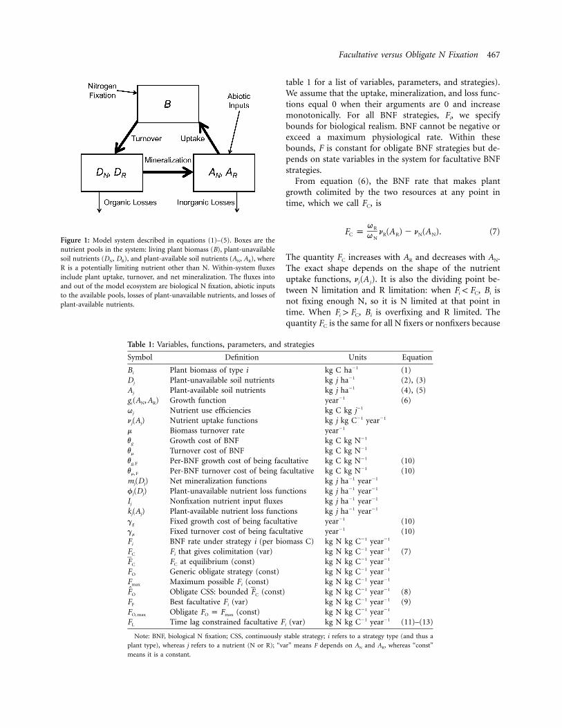
Bi (in units of mass or carbon per area) of different N-fixer types i (with BNF rates Fi), organically bound N (DN)and another nutrient (DR, where R is a generic resource,which could be phosphorus, P, or any other soil-derivedresource) in soil detritus, and the plant-available forms ofN (AN) and the other resource (AR; fig. 1).

The model works for an arbitrary number of N-fixertypes, but we will generally consider only one or two inour analyses. The growth rate for each type, ,g (A , A )i N R

depends on acquisition of the two resources (through up-take from the soil, , and/or BNF, Fi) and the nutrientn (A )j j

use efficiencies (NUEs), qj (equivalent to the biomass-to-nutrient or carbon-to-nutrient ratios of litter; Vitousek1982). Growth is governed by Liebig’s law of the minimumfunction (e.g., Von Liebig 1840; Tilman 1982), so it canbe limited by a single nutrient or by both at certain points.Plant turnover occurs at a base rate, m, and is augmentedby increasing BNF. The costs of BNF, vg and vm, are im-plemented as a decrease in the growth rate and an increasein the turnover rate, respectively (both proportional to therate of BNF). This formulation reflects trade-offs betweenBNF and nutrient uptake, NUE, and turnover (similar toMenge et al. 2008).

The model satisfies the equations

dBi p B [g (A , A ) � (m � v F)], (1)i i N R m idt

dD (m � v F)BN m i ip � m (D ) � f (D ), (2)� N N N Ndt qi N

dD (m � v F)BR m i ip � m (D ) � f (D ), (3)� R R R Rdt qi R

dAN p I � k (A ) � m (D )N N N N Ndt

Bi� [g (A , A ) � q F], (4)� i N R N iqi N

dAR p I � k (A ) � m (D )R R R R Rdt

Bi� g (A , A ), (5)� i N Rqi R

g (A , A ) p min {q [n (A ) � F], q n (A )}i N R N N N i R R R

� v F . (6)g i

In addition to the variables and parameters describedabove, mj(Dj) are the mineralization functions, fj(Dj) arethe organic loss functions, Ij are the abiotic nutrient inputs,and kj(Aj) are the available nutrient loss functions (see

Facultative versus Obligate N Fixation 467

Figure 1: Model system described in equations (1)–(5). Boxes are thenutrient pools in the system: living plant biomass (B), plant-unavailablesoil nutrients (DN, DR), and plant-available soil nutrients (AN, AR), whereR is a potentially limiting nutrient other than N. Within-system fluxesinclude plant uptake, turnover, and net mineralization. The fluxes intoand out of the model ecosystem are biological N fixation, abiotic inputsto the available pools, losses of plant-unavailable nutrients, and losses ofplant-available nutrients.

Table 1: Variables, functions, parameters, and strategies

Symbol Definition Units Equation

Bi Plant biomass of type i kg C ha�1 (1)Dj Plant-unavailable soil nutrients kg j ha�1 (2), (3)Aj Plant-available soil nutrients kg j ha�1 (4), (5)g (A , A )i N R Growth function year�1 (6)qj Nutrient use efficiencies kg C kg j�1

(Aj)nj Nutrient uptake functions kg j kg C�1 year�1

m Biomass turnover rate year�1

vg Growth cost of BNF kg C kg N�1

vm Turnover cost of BNF kg C kg N�1

vg, F Per-BNF growth cost of being facultative kg C kg N�1 (10)vm, F Per-BNF turnover cost of being facultative kg C kg N�1 (10)mj(Dj) Net mineralization functions kg j ha�1 year�1

fj(Dj) Plant-unavailable nutrient loss functions kg j ha�1 year�1

Ij Nonfixation nutrient input fluxes kg j ha�1 year�1

kj(Aj) Plant-available nutrient loss functions kg j ha�1 year�1

gg Fixed growth cost of being facultative year�1 (10)gm Fixed turnover cost of being facultative year�1 (10)Fi BNF rate under strategy i (per biomass C) kg N kg C�1 year�1

FC Fi that gives colimitation (var) kg N kg C�1 year�1 (7)FC FC at equilibrium (const) kg N kg C�1 year�1

FO Generic obligate strategy (const) kg N kg C�1 year�1

Fmax Maximum possible Fi (const) kg N kg C�1 year�1

FO Obligate CSS: bounded (const)FC kg N kg C�1 year�1 (8)FF Best facultative Fi (var) kg N kg C�1 year�1 (9)FO, max Obligate (const)F p FO max kg N kg C�1 year�1

FL Time lag constrained facultative Fi (var) kg N kg C�1 year�1 (11)–(13)

Note: BNF, biological N fixation; CSS, continuously stable strategy; i refers to a strategy type (and thus a

plant type), whereas j refers to a nutrient (N or R); “var” means F depends on AN and AR, whereas “const”

means it is a constant.

table 1 for a list of variables, parameters, and strategies).We assume that the uptake, mineralization, and loss func-tions equal 0 when their arguments are 0 and increasemonotonically. For all BNF strategies, Fi, we specifybounds for biological realism. BNF cannot be negative orexceed a maximum physiological rate. Within thesebounds, F is constant for obligate BNF strategies but de-pends on state variables in the system for facultative BNFstrategies.

From equation (6), the BNF rate that makes plantgrowth colimited by the two resources at any point intime, which we call FC, is

qRF p n (A ) � n (A ). (7)C R R N NqN

The quantity FC increases with AR and decreases with AN.The exact shape depends on the shape of the nutrientuptake functions, . It is also the dividing point be-n (A )j j

tween N limitation and R limitation: when , Bi isF ! Fi C

not fixing enough N, so it is N limited at that point intime. When , Bi is overfixing and R limited. TheF 1 Fi C

quantity FC is the same for all N fixers or nonfixers because


all types have access to the same resource pools and be-cause we assumed that stoichiometries and uptake ratesdo not differ between types (we assumed this to isolatethe effects of different strategies from other potential dif-ferences between types). We will also refer to , the con-FC

stant BNF rate that gives colimitation at equilibrium (FC

evaluated at , ). Mathematically, both FC and canA A FN R C

be negative or arbitrarily high, which is biologically un-realistic. Therefore, FC and can be BNF strategies onlyFC

when modified to remain within biologically sensiblebounds (table 1).

Model Analysis

We use a combination of techniques to examine how thedifferent BNF strategies compare against each other. Tocompare obligate BNF strategies against each other in anequilibrium environment, we search for evolutionarily sta-ble (cannot be invaded once established), convergence sta-ble (will be evolutionarily approached from anywhere),and continuously stable (both evolutionarily and conver-gence stable) strategies (Eshel 1983; Geritz et al. 1997;Levin and Muller-Landau 2000). These techniques fromadaptive dynamics (Geritz et al. 1998) assume that a strat-egy that is constant over ecological time (like obligate BNF)can change over evolutionary time and that ecological sys-tems come to equilibrium between evolutionary events(e.g., mutations in the population). When these assump-tions are met, these are powerful analytical techniques,allowing us to determine which types will evolve and out-compete other types.

However, these assumptions are not always met. Bio-geochemical systems can take a long time to equilibrate(Walker and Syers 1976; Vitousek 2004; Menge et al. 2009),and we are interested in the dynamics of different BNFstrategies in transient environments as well as equilibriumenvironments. To compare different types against eachother in transient environments, we first compute the rel-ative growth rates (RGRs), . This technique is(1/B )(dB /dt)i i

less powerful than adaptive dynamics but has many fewerassumptions (notably, it is relevant everywhere rather thanonly at equilibrium). In certain conditions, comparingRGRs is quite powerful: if one type always has a higherRGR than another type, it will eventually drive the othertype to extinction if they are limited by the same nutrient(including one type being colimited). However, if the rankof RGRs differs under different environmental conditions,there is no clear winner in fluctuating environments. Toillustrate possible outcomes in these unclear cases andcomplement the analytical results, we simulate the systemwith Matlab’s ode45 and dde23 functions, using realisticparameter values (parameterizing R as phosphorus) and

starting conditions (found in the appendix in the onlineedition of the American Naturalist).

To examine the environmental impacts of different BNFstrategies, we determine how available N loss rates dependon BNF strategies, using equilibrium and quasi-equilib-rium analyses as well as simulations. Equilibrium loss ratesare easy to calculate, depend only on parameters in thesystem, and would be observed in ecosystems that havebeen undisturbed for at least many centuries, such as ma-ture forests without fire, large storms, or other large-scaledisturbances (Menge et al. 2009). However, many ecosys-tems have much shorter disturbance return intervals, soto investigate loss rates in these ecosystems we calculateshort timescale quasi-equilibrium loss rates (as in Mengeet al. 2009). The quasi-equilibrium analysis assumes thatavailable nutrients in the soil track biomass and soil or-ganic matter, which happens within hours to weeks (Jack-son et al. 1989; Schimel et al. 1989; Perakis and Hedin2001; Providoli et al. 2006) and thus is relevant for eco-systems that have been undisturbed for this shorter period.However, unlike equilibrium analyses, quasi-equilibriumanalyses depend on the current state of biomass and or-ganically bound soil nutrients and thus require differentinformation. As with the competition analysis, we com-plement the analytical loss results by simulating the systemto illustrate numerically the effects of different BNF strat-egies on plant-available N losses.

Results

If the costs of BNF ( ) exceed the benefits (qN),v � v p vg m

there is obviously no advantage to BNF, and obligate non-fixers always exclude any N fixer. Because our purposehere is to compare different types of N fixers, we hereafterassume that .q 1 vN

Obligate BNF

In an equilibrium environment, the continuously stablestrategy (CSS) for obligate N fixers is the constant BNFrate that yields colimitation at equilibrium when possible,

�F p min (F , F ). (8)O maxC

Here, indicates if it is positive and 0 if it is not. The�F FC C

CSS may range from nonfixation (0) to the maximalFO

BNF rate ( ). Following the definition of CSS, this typeFmax

will be approached evolutionarily from any starting pointand will not be invaded (see the appendix for details ofthe CSS analysis).

Although this is a clear answer for equilibrium envi-ronments, terrestrial ecosystem nutrient cycles take a long


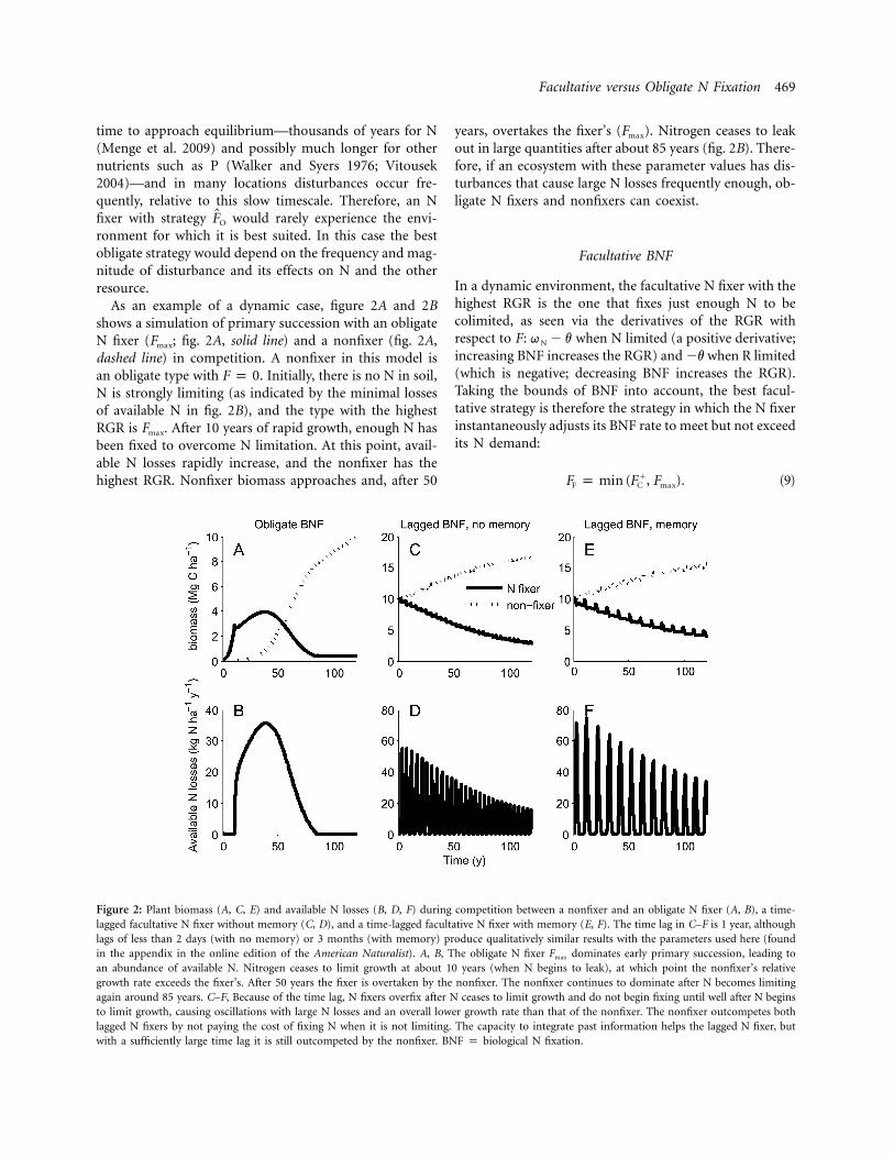
Figure 2: Plant biomass (A, C, E) and available N losses (B, D, F) during competition between a nonfixer and an obligate N fixer (A, B), a time-lagged facultative N fixer without memory (C, D), and a time-lagged facultative N fixer with memory (E, F). The time lag in C–F is 1 year, althoughlags of less than 2 days (with no memory) or 3 months (with memory) produce qualitatively similar results with the parameters used here (foundin the appendix in the online edition of the American Naturalist). A, B, The obligate N fixer dominates early primary succession, leading toFmax

an abundance of available N. Nitrogen ceases to limit growth at about 10 years (when N begins to leak), at which point the nonfixer’s relativegrowth rate exceeds the fixer’s. After 50 years the fixer is overtaken by the nonfixer. The nonfixer continues to dominate after N becomes limitingagain around 85 years. C–F, Because of the time lag, N fixers overfix after N ceases to limit growth and do not begin fixing until well after N beginsto limit growth, causing oscillations with large N losses and an overall lower growth rate than that of the nonfixer. The nonfixer outcompetes bothlagged N fixers by not paying the cost of fixing N when it is not limiting. The capacity to integrate past information helps the lagged N fixer, butwith a sufficiently large time lag it is still outcompeted by the nonfixer. BNF p biological N fixation.

time to approach equilibrium—thousands of years for N(Menge et al. 2009) and possibly much longer for othernutrients such as P (Walker and Syers 1976; Vitousek2004)—and in many locations disturbances occur fre-quently, relative to this slow timescale. Therefore, an Nfixer with strategy would rarely experience the envi-FO

ronment for which it is best suited. In this case the bestobligate strategy would depend on the frequency and mag-nitude of disturbance and its effects on N and the otherresource.

As an example of a dynamic case, figure 2A and 2Bshows a simulation of primary succession with an obligateN fixer ( ; fig. 2A, solid line) and a nonfixer (fig. 2A,Fmax

dashed line) in competition. A nonfixer in this model isan obligate type with . Initially, there is no N in soil,F p 0N is strongly limiting (as indicated by the minimal lossesof available N in fig. 2B), and the type with the highestRGR is . After 10 years of rapid growth, enough N hasFmax

been fixed to overcome N limitation. At this point, avail-able N losses rapidly increase, and the nonfixer has thehighest RGR. Nonfixer biomass approaches and, after 50

years, overtakes the fixer’s ( ). Nitrogen ceases to leakFmax

out in large quantities after about 85 years (fig. 2B). There-fore, if an ecosystem with these parameter values has dis-turbances that cause large N losses frequently enough, ob-ligate N fixers and nonfixers can coexist.

Facultative BNF

In a dynamic environment, the facultative N fixer with thehighest RGR is the one that fixes just enough N to becolimited, as seen via the derivatives of the RGR withrespect to F: when N limited (a positive derivative;q � vN

increasing BNF increases the RGR) and �v when R limited(which is negative; decreasing BNF increases the RGR).Taking the bounds of BNF into account, the best facul-tative strategy is therefore the strategy in which the N fixerinstantaneously adjusts its BNF rate to meet but not exceedits N demand:

�F p min (F , F ). (9)F C max


Obligate versus Facultative BNF

The RGR of the best facultative N fixer (FF) matches orexceeds that of any obligate N fixer, as shown in the ap-pendix. In this simple model, a facultative N fixer caninvade and exclude any obligate N fixer, but some N fixersin real ecosystems seem to be obligate. Why might obligateN fixers exist? One option is that they have not evolvedthe capability of being facultative, but this answer is hardlysatisfying. In the next two sections, we examine two phys-iological mechanisms that could give obligate types anadvantage: fixed costs of being facultative and time lagsinherent to BNF.

Costs of Being Facultative

To adjust BNF to local environmental conditions, it isnecessary to respond to the environment (or some indexthereof, such as internal nutrient stores in a plant) and tohave the physiological machinery to increase or decreasethe rate of BNF. Such infrastructure may carry a cost (vanKleunen and Fischer 2005), which would result in a fixedcost that decreases the growth rate (or increases the turn-over rate or both) regardless of the amount of BNF. It isalso possible that the per-unit cost of BNF is higher forfacultative N fixers. For example, changing the BNF ratecould involve the creation/destruction of nodules or theactivation/deactivation of symbionts, which may carry agreater cost than for obligate N fixers that keep a steadynodule density or activity level. Here we examine howthese costs of being facultative, which could arise fromthese mechanisms or others, influence competition be-tween a facultative N fixer and an obligate N fixer.

Let there be fixed and variable costs of being facultativethat decrease the growth rate (gg and ) and increase thevg, F

turnover rate (gm and ). Defining andv g { g � gm, F g m

(i.e., combining the growth and mortalityv { v � vF g, F m, F

costs, which have identical effects on the analyses we pre-sent here), the rate of change of BF is now

dBF p B (min {q [n (A ) � F ], q n (A )}F N N N F R R Rdt

� m � (v � v )F � g). (10)F F

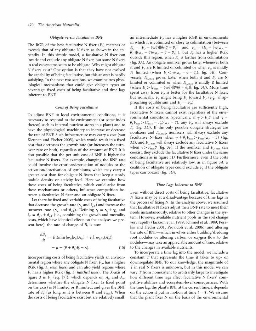
Incorporating costs of being facultative yields an environ-mental region where any obligate N fixer, FO, has a higherRGR (fig. 3, solid lines) and can also yield regions whereFF has a higher RGR (fig. 3, hatched lines). The X-axis offigure 3 is FC (eq. [7]), which depends on AN and AR,determines whether the obligate N fixer (a fixed pointon the axis) is N limited or R limited, and gives the BNFrate of FF (as long as it is between 0 and ). WhenFmax

the costs of being facultative exist but are relatively small,

an intermediate FO has a higher RGR in environmentsin which it is colimited or close to colimitation (between

andF p [F � (g/v)][v/(v � v )] F p {F � [g/(q �C O F C O N

), but FF has a higher RGRv)]}[(q � v)/(q � v � v )]N N F

outside this region, when FO is farther from colimitation(fig. 3A). An obligate nonfixer grows faster whenever bothit and FF are R limited or colimited or when FO is mildlyN limited (when ; fig. 3B). Con-F ! g/(q � v � v )C N F

versely, grows faster when both it and FF are NFO, max

limited or colimited or when is mildly R limitedFO, max

(when ; fig. 3C). More timeF 1 [F � (g/v)][v/(v � v )]C max F

spent away from FO is better for the facultative N fixer,but ironically, FF might bring FC toward FO (e.g., if ap-proaching equilibrium and ).ˆF p FO O

If the costs of being facultative are sufficiently high,facultative N fixers cannot exist regardless of the envi-ronmental conditions. Specifically, if andg 1 F v g �O

, any FO will always excludev F 1 (F � F )(q � v)F max max O N

FF (fig. 3D). If the only possible obligate strategies arenonfixers and , nonfixers will always exclude anyFO, max

facultative N fixer when (fig.g � v F 1 F (q � v)F max max N

3E), and will always exclude any facultative N fixersFO, max

when (fig. 3F). If the nonfixer and cang 1 F v Fmax O, max

coexist, they exclude the facultative N fixer under the sameconditions as in figure 3D. Furthermore, even if the costsof being facultative are relatively low, as in figure 3A, acoalition of obligate types could exclude FF if the obligatetypes can coexist (fig. 3G).

Time Lags Inherent to BNF

Even without direct costs of being facultative, facultativeN fixers may be at a disadvantage because of time lags inthe process of fixing N. In the analysis above, we assumedthat facultative N fixers adjust their BNF rate to meet theirneeds instantaneously, relative to other changes in the sys-tem. However, available nutrient pools in the soil changevery rapidly (Jackson et al. 1989; Schimel et al. 1989; Pera-kis and Hedin 2001; Providoli et al. 2006), and alteringthe rate of BNF—which involves either building/sheddingroot nodules or altering carbon or oxygen flow to thenodules—may take an appreciable amount of time, relativeto the changes in available nutrients.

To incorporate a time lag into the model, we include aconstant T that represents the time it takes to up- ordownregulate BNF. To our knowledge, the magnitude ofT in real N fixers is unknown, but in this model we canvary T from nonexistent to arbitrarily large to investigatehow different time lags affect facultative N fixers’ com-petitive abilities and ecosystem-level consequences. Withthe time lag, the plant’s BNF at the current time, t, dependson the action it put in motion at time . We assumet � Tthat the plant fixes N on the basis of the environmental


Figure 3: Effects of costs of being facultative on relative growth rates (RGRs) of obligate versus facultative types (i.e., N fixers or nonfixers). TheX-axis is FC (eq. [7]), the amount of fixation needed to be colimited, which changes with the environment: it decreases as soil N increases andincreases as the other resource (R) increases. When , Bi is underfixing and N limited, whereas when , it is overfixing and R limited.F ! F F 1 Fi C i C

The quantity FC can be negative or above , but Fi cannot, so the facultative N fixer we consider, FF, equals FC where possible but is boundedFmax

by 0 and . Obligate N fixers, FO, are constant points on the FC axis. Solid lines indicate a higher RGR for FO, whereas hatched lines indicate aFmax

higher RGR for FF. The constants, which indicate the cost of being facultative, are , , , andc p g/v c p v/(v � v ) c p g/(q � v) c p (q �1 2 F 3 N 4 N

. When FF pays a fixed cost g or a variable cost vF of being facultative, it can have a higher RGR when FC is sufficiently far fromv)/(q � v � v )N F

FO (A–C), but if g or vF are sufficiently high relative to the net gain of fixing N, FF always has a lower RGR (D–G). For instance, in B, the obligatetype is a nonfixer. If soil N and R availability are such that the nonfixer would be R limited ( ), the nonfixer has a higher RGR because,F ! 0C

although neither it nor the facultative type is fixing, the facultative type pays a cost to be facultative. If soil N and R availability are such that thenonfixer is weakly N limited relative to the cost of being facultative ( ), the nonfixer still has a higher RGR, but if the nonfixer is strongly0 ! F ! c cC 3 4

N limited relative to the cost of being facultative ( ), the facultative fixer has a higher RGR.0 ! c c ! F3 4 C

conditions at or before and let the constrained fac-t � Tultative N fixer, FL, (L for lag) fix N in such a way as tobalance the resource availabilities about which it has in-formation. The simplest extension of the unlagged fac-ultative fixer FF is that FL fixes enough N at t such that itwould be colimited at :t � T

�F (t) p min (F (t � T) , F ). (11)L C max

Alternatively, plants may have the capacity to integratepast information, for example, if internal nutrient storesare used to regulate BNF, and they depend on nutrientavailabilities before . We call this integration of pastt � Tinformation “memory,” for lack of a better term. To in-clude memory in the model, we let FL fix N so as to balancethe resource availabilities from before to ,t � T t � T

weighting information from the recent past more than thedistant. If l is the discounting/weighting factor, theamount fixed at time ist

t�T

�l(t�T�t)F (t) p F (t)le dt, (12)L � C��

which is still subject to the bounds of 0 and . EquationFmax

(11) is a special case of equation (12). Differentiating equa-tion (12) gives

dFL p l[F (t � T) � F ]. (13)C Ldt

Equation (13) can be coupled to equations (1)–(5), with


FL (from eq. [12]) in place of F and with appropriate initialconditions, to make a set of delayed differential equations.It is not trivial to determine the optimal (or evolutionarily/convergence stable) facultative BNF strategy with the timelag constraint, and we make no claim that either versionof FL we present here is the best strategy. However, theyare useful comparisons with FF and FO.

Unlike the unconstrained facultative N fixer FF, FL (withor without memory) is unlikely to be colimited at anygiven point in time. Which nutrient limits FL depends onthe history of nutrients in the soil as well as the currentstate. As shown in the appendix, the time-lagged facultativeN fixer (FL) never has a RGR higher than that of theunlagged facultative N fixer (FF). Compared with an ar-bitrary obligate N fixer FO, FL may have a higher or lowerRGR at any point in time, and therefore the competitiveoutcome is not immediately clear. If T is small and therecent information is strongly weighted, FL is similar to FF

and therefore is likely to outcompete FO. However, if theinherent time lag T is quite large, FL is less likely to out-compete FO and can even be outcompeted by FO.

As our simulations demonstrate, sufficiently large timelags can permit an obligate nonfixer to outcompete time-lagged facultative N fixers without (fig. 2C, 2D) and with(fig. 2E, 2F) memory. (By “outcompete,” we mean that itgrows to a higher biomass level. We have proven nothingabout coexistence, and simulations suggest that FL caninvade when it is rare, even in many scenarios in whichit is outcompeted.) In figure 2C–2F the time lag is 1 year,which means that the N fixer adjusts its N fixation to meetthe demand it had last year. This leads to pronounceddifferences in growth between the obligate nonfixer andlagged facultative N fixers (fig. 2C, 2E), as well as large Nlosses (fig. 2D, 2F). As has been known for some time(Cunningham 1954), sufficiently large time lags can de-stabilize otherwise stable systems. In our system as well,the time lag produces oscillations. The lagged facultativefixer continues fixing N after it is no longer N limited,then stops fixing N, and does not fix N again until it hasbeen N limited for a period equal to the delay. This con-sistent overfixing or underfixing leads to its lower com-petitive ability (fig. 2C, 2E) and high N losses (fig. 2D,2F).

Time lags much smaller than a year can also permit anobligate type to outcompete a lagged N fixer, even whenthere are no direct costs of being facultative. With a re-alistic set of parameters and starting conditions (see ap-pendix), simulations reveal that the threshold lags thatdetermine whether a nonfixer (one particular obligatetype) outgrows FL are between 1 and 2 days when FL hasno memory and 2 and 3 months when FL has memory.For the large range of the memory effect parameter wetried (l ranging from 10�4 to 104 year�1, lags ranging from

a minute to a year), having memory consistently improvesthe competitive ability of FL since the threshold time lagthat determines whether FL outcompetes the nonfixer wasconsistently higher when FL had memory.

Effects of BNF Strategy and Time Lags onAvailable N Losses

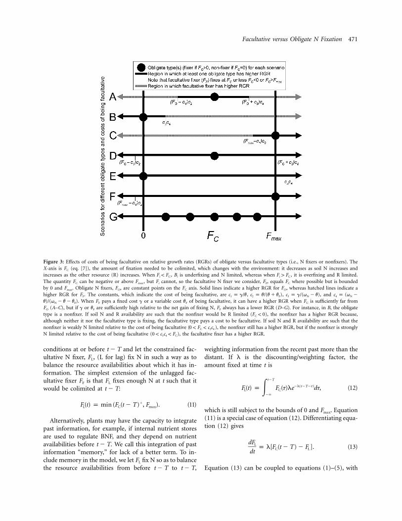
Now that we have a sense for the effects of BNF strategyon competition, we investigate how the different strategiesinfluence a fundamental ecosystem property and a keyindex of N richness: losses of available N from the soil.At equilibrium, available N losses in a system with an N-limited obligate N fixer slightly decrease as BNF increases.This happens because BNF increases equilibrium biomass,which drives slightly lower. When an obligate N fixerAN

is R limited, equilibrium N losses increase dramaticallywith increasing BNF for realistic parameters (see the ap-pendix for details of these analyses). The whole equilib-rium picture (fig. 4A), therefore, shows that available Nlosses decline very slightly with rising BNF until F pO

(the kink) and then rise with overfixation. Figure 4AFC

shows the effect of varying amounts of BNF on plant-available N losses at equilibrium (solid line) and quasiequilibrium (dotted lines, for two different states of plantbiomass and soil organic nutrients) for a realistic set ofparameters, flux functions, and starting conditions (seeappendix). In each line the kink is at FC, that is, wherelimitation switches from N limitation to R limitation andwhere the facultative N fixer FF would be.

Many forests are not at the long-term equilibrium ofthis model, so we also examined N loss rates at quasiequilibrium, when soil-available nutrients are assumed toequilibrate rapidly relative to soil organic matter and plantbiomass. When the plant is N limited, quasi-equilibriumN losses increase slightly with BNF. (The decrease seen inthe equilibrium case results from longer-term feedbacksof increased biomass with BNF.) When an obligate N fixeris R limited, quasi-equilibrium N losses rise substantiallywith BNF, as illustrated in the dotted lines in figure 4A tothe left (N limited) and the right (R limited) of the kinkat (see appendix for details).F p FO C

In the higher dotted line in figure 4A, plants need tofix N only at a miniscule rate to be colimited (the kinkin the curve is at approximately 0.005 mg N g C�1 year�1)because the N-to-R ratio in soil organic matter (miner-alized and made available to the plant population) is higherthan at equilibrium. Therefore, obligate N fixers with ahigher BNF rate (such as 0.025 mg N g C�1 year�1, whichwould give colimitation at equilibrium) would be R limitedand allow about 3 kg N ha�1 year�1 to be lost as availableN. The lower dotted line represents a state of the systemthat is more N poor than at equilibrium, as might be seen


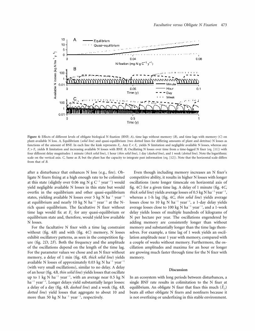
Figure 4: Effects of different levels of obligate biological N fixation (BNF; A), time lags without memory (B), and time lags with memory (C) onplant-available N loss. A, Equilibrium (solid line) and quasi-equilibrium (two dotted lines for differing amounts of plant and detritus) N losses asfunctions of the amount of BNF. In each line the kink represents FC. Any yields N limitation and negligible available N losses, whereas anyF ! Fi C

yields R limitation and increasing available N losses with BNF. B, Oscillating N losses over time from a time-lagged N fixer (eq. [11]) withF 1 Fi C

four different delay magnitudes: 1 minute (thick solid line), 1 hour (thin solid line), 1 day (dashed line), and 1 week (dotted line). Note the logarithmicscale on the vertical axis. C, Same as B, but the plant has the capacity to integrate past information (eq. [12]). Note that the horizontal scale differsfrom that of B.

after a disturbance that enhances N loss (e.g., fire). Ob-ligate N fixers fixing at a high enough rate to be colimitedat this state (slightly over 0.06 mg N g C�1 year�1) wouldyield negligible available N losses in this state but wouldoverfix in the equilibrium and other quasi-equilibriumstates, yielding available N losses over 5 kg N ha�1 year�1

at equilibrium and nearly 10 kg N ha�1 year�1 at the N-rich quasi equilibrium. The facultative N fixer withouttime lags would fix at FC for any quasi-equilibrium orequilibrium state and, therefore, would yield low availableN losses.

For the facultative N fixer with a time lag constraintwithout (fig. 4B) and with (fig. 4C) memory, N lossesexhibit oscillatory patterns, as seen in the competition fig-ure (fig. 2D, 2F). Both the frequency and the amplitudeof the oscillations depend on the length of the time lag.For the parameter values we chose and an N fixer withoutmemory, a delay of 1 min (fig. 4B, thick solid line) yieldsavailable N losses of approximately 0.03 kg N ha�1 year�1

(with very small oscillations), similar to no delay. A delayof an hour (fig. 4B, thin solid line) yields losses that oscillateup to 1 kg N ha�1 year�1, with an average near 0.5 kg Nha�1 year�1. Longer delays yield substantially larger losses:a delay of a day (fig. 4B, dashed line) and a week (fig. 4B,dotted line) yield losses that aggregate to about 10 andmore than 50 kg N ha�1 year�1, respectively.

Even though including memory increases an N fixer’scompetitive ability, it results in higher N losses with longeroscillations (note longer timescale on horizontal axis offig. 4C) for a given time lag. A delay of 1 minute (fig. 4C,thick solid line) yields average losses of 0.5 kg N ha�1 year�1,whereas a 1-h lag (fig. 4C, thin solid line) yields averagelosses close to 10 kg N ha�1 year�1, a 1-day delay yieldsaverage losses close to 100 kg N ha�1 year�1, and a 1-weekdelay yields losses of multiple hundreds of kilograms ofN per hectare per year. The oscillations engendered byadding memory are consistently longer than withoutmemory and substantially longer than the time lags them-selves. For example, a time lag of 1 week yields an oscil-lation amplitude near 1 year with memory, compared witha couple of weeks without memory. Furthermore, the os-cillation amplitudes and maxima for an hour or longerare growing much faster through time for the N fixer withmemory.

Discussion

In an ecosystem with long periods between disturbances, asingle BNF rate results in colimitation to the N fixer atequilibrium. An obligate N fixer that fixes this much ( )FO

beats all other obligate N fixers and nonfixers because itis not overfixing or underfixing in this stable environment.


In dynamic or transient environments, however, the bestobligate BNF strategy is not clear, and facultative N fixersare more likely to win as long as the costs of being fac-ultative are small. In fact, if BNF can be adjusted veryrapidly, one type of facultative N fixer always fixes justenough to be colimited by N and another resource. Thisstrategy (FF) also yields very small N losses because it neveroverfixes. If there are no costs to being facultative, FF isequivalent to the best obligate type in a stable environmentand superior to any obligate type in dynamic environmentsbecause it is colimited whenever possible.

Although facultative N fixers always win in the simplestmodel, including costs of being facultative or time lagsinherent to facultative BNF in the model can have strongeffects on the competitive ability of facultative N fixers.Two types of cost we investigated were a fixed cost of beingfacultative and a variable cost of being facultative thatincreases the per-unit cost of BNF. A fixed cost could arisefrom the need to have infrastructure to sense and respondto the environment. All plants have such infrastructurefor certain functions (e.g., stomatal guard cells that openand close in response to light and water availability), andthe capacity to alter BNF may require additional infra-structure that would carry fixed structural, respiration, andopportunity costs. Facultative N fixers may also havehigher per-unit costs of BNF. For example, building nod-ules requires carbon for structure as well as the metaboliccost of fixing N, and facultative N fixers that turn noduleson and off may be paying a higher structural cost per unitof N fixed than are obligate N fixers that keep their nodulesfor long periods. These costs of being facultative, if theyare large enough, can prevent facultative BNF from evolv-ing or succeeding. Therefore, these costs can also result inlarge N losses or severe N limitation because the successof obligate N fixers means overfixation in certain envi-ronments and underfixation in others.

Time lags inherent to BNF can also hinder the com-petitive ability of facultative N fixers and affect ecosystem-level N dynamics. Building nodules and altering carbonflow to nodules takes time, so adjusting BNF cannot beinstantaneous. Because of feedbacks and delays amongBNF, litterfall, and decomposition, even small lags in BNFcan severely hinder the competitive ability of facultativeN fixers. Moreover, because lags induce periods of N sat-uration to the plant as large quantities of N are beingliberated from decomposing organic matter, and, con-versely, periods of N starvation before BNF is active, theycan lead to large losses of plant-available N and periodsof severe N limitation, much like obligate N fixers. There-fore, both lagged facultative N fixers and obligate N fixerscan push an ecosystem over thresholds into N richness orN limitation, with a key difference in timescale. FacultativeN fixers adjust BNF on physiological timescales, which are

much shorter than the timescale of community dynamicsat which obligate BNF strategies affect N dynamics.

In addition to the costs we considered and time lags, aconstraint on BNF that we did not include in our modelmay also affect N dynamics and the fitness of facultativeN fixers. Rapid changes in the rate of BNF may be costlybecause of the construction cost of nodules, above andbeyond the higher per-unit BNF cost we examined here.If this is true, an explicit incorporation of the cost ofchanging the BNF rate would likely reinforce our resultthat obligate N fixers can outcompete facultative N fixersif the cost of being facultative is high enough. However,it could also result in a benefit to certain types of timelags, which our current model does not allow. In particular,a condition that specifies that the plant waits for a largechange in soil nutrient conditions before adjusting BNFcould yield fewer large swings in BNF than are seen ininstantaneously adjusting BNF to be colimited. In this caseit is also possible that an intermediate lag is most beneficial.

Other model omissions may also affect our results andshould be examined in future studies. For instance, dis-tinguishing between fine roots and other plant tissues,including the possibility of light limitation, allowing plantstoichiometry to be flexible, and using more detailedgrowth equations would be more realistic and may altercyclical dynamics or cost/benefit calculations. Despitethese simplifications, our model results may shed light onBNF strategies and biome-level nutrient and biogeographicpatterns.

Our model suggests that, without any constraints, allplants should be facultative N fixers. The constraints weexamine here—which are by no means the only possibleconstraints—allow a much richer array of BNF strategies,as seems to occur in nature, and a correspondingly richarray of ecosystem N dynamics. Although some of thepatterns themselves are poorly known (e.g., BNF strategiesemployed by different organisms in different biomes) andthere are other potential explanations for biome-level dif-ferences (Houlton et al. 2008), we now speculate on theextent to which costs of being facultative and time lagsinherent to BNF could influence biome-level patterns ofBNF and N dynamics.

Temperate and Boreal Forest Pattern

The successional pattern in temperate and boreal forestsis consistent with the following scenario: no facultative Nfixer can invade any system because the costs of beingfacultative are sufficiently high (as in fig. 3D–3F). Early insuccession, when N is strongly limiting, an obligate N fixerfixing at the maximal rate has the highest RGR, so it dom-inates early successional habitats (fig. 2A). As it brings Ninto the system, the limiting nutrient flips from N to R,


at which point available N starts leaking in large quantities(fig. 2B; as seen in Binkley et al. 1992; Compton et al.2003). As limitation switches from N to R, nonfixers havea higher RGR because they are not paying BNF costs. Sometime after this switch in limitation, on the timescale ofcommunity dynamics, nonfixers overtake obligate N fixersand become dominant (fig. 2A). Without the BNF input,uncontrollable N losses bring N limitation back as theforest ages, and available N losses decrease to a minimumin a mature forest (fig. 2B; Hedin et al. 1995). This by nomeans proves that these mechanisms cause these patterns,but the extent to which the model results agree with ob-served patterns warrants further investigation into morepoorly known aspects, such as whether actinorhizal N fix-ers are indeed obligate and the costs of being facultative.

Tropical Forest Pattern

The pattern starting to emerge in tropical forests—fac-ultative N fixers coexisting with nonfixers and high avail-able N losses (Jenny 1950; Vitousek et al. 2002; Hedin etal. 2003; Barron 2007)—is consistent with a time lag effect,and costs of being facultative could also play a role. Eitherconstraint, if it has a moderate effect, could potentiallyallow coexistence over some time interval since both typeshave a higher RGR in certain regions of nutrient avail-ability. For instance, if there is a small cost of being fac-ultative (as in fig. 3A–3C), facultative N fixers would havethe advantage in newly disturbed areas (such as treefallgaps) where N limitation is more likely. In undisturbed,N-rich areas, obligate nonfixers would have a higher RGR,even if the facultative N fixers are not fixing N (so longas there is a fixed cost of being facultative).

Time lags can also explain the coexistence of facultativeN fixers with nonfixers (e.g., in fig. 2C, 2E both typescoexist for a long time) and could explain the N richnessseen in tropical forests (figs. 2D, 2F, 4B, 4C). Even a smalltime lag in facultative BNF produces substantial overfix-ation. In any given location this overfixation emerges aspulses in N richness following switches from N to R lim-itation (fig. 4B, 4C), but averaged over a landscape thiscould produce chronic N richness. Given the large effectof the time lag magnitude on N losses and the competitiveability of facultative N fixers, studies investigating the valueof this time lag are sorely needed.

Why Facultative BNF in the Tropics and ObligateBNF in Temperate/Boreal Zones?

According to our model, costs of being facultative andtime lags inherent to BNF can produce the patterns ofobligate BNF in temperate/boreal forests and facultativeBNF in tropical forests. To explain both patterns simul-

taneously, at least one of the constraints must be relativelygreater outside the tropics. Two key differences in the twobiomes may affect the magnitude of costs or time lags.First, because tropical forests are nearer the equator, theygenerally have higher temperatures and longer growingseasons than their poleward counterparts. Second, thedominant N-fixing symbioses differ phylogenetically: le-gumes with rhizobia dominate in the tropics, whereas ac-tinorhizal symbioses between nonleguminous plants andactinomycete bacteria are more common in temperate andboreal forests.

Environmental effects may influence time lags and costsof being facultative. Enzyme activity depends on temper-ature, and because all processes involved in up- or down-regulating N fixation must depend on enzymes, coldertemperatures away from the equator may push facultativeN fixation over a threshold from net benefit to net cost.Given that the realized cost of being facultative dependson the maximum BNF rate ( ; fig. 3), lower inF Fmax max

lower temperatures may also render being facultative morecostly. On a longer timescale, even if it takes a similaramount of time to build nodules in tropical and temperateforests, shorter growing seasons away from the equatormay disfavor facultative nodulation because the active pe-riod is shorter relative to the building period.

Both partners in the symbiosis and the symbiotic struc-ture itself (the nodule) differ between the two types ofsymbiosis (Huss-Danell 1997). Actinorhizal nodules areharder than rhizobial nodules and can be large, occasion-ally exceeding a 5-cm diameter (D. Menge, personal ob-servation). This suggests that they may take longer to buildor shed than the softer rhizobial nodules, consistent witha longer time lag in actinorhizal symbioses. Because theinterior environment (in particular the oxygen content,which is known to be a key control on nitrogenase effi-ciency; Leigh 2002) of the actinorhizal nodule is less wellregulated than that of the rhizobial nodule, the effectivecost of each unit of BNF may also be higher for actinorhizalsymbioses. Any combination of a longer time lag and ahigher per-unit N cost of BNF in actinorhizal symbioses—if sufficiently large—could explain the difference betweentropical and temperate forests. However, this is a proxi-mate (as opposed to ultimate) explanation since it doesnot explain the biogeography of each symbiosis or whythe actinorhizal and rhizobial structures differ. These maybe because of historical accidents but may also be becauseof deterministic environmental effects such as those men-tioned above.

Leguminous N-fixing trees exist in temperate zones(e.g., Robinia pseudoacacia [black locust]), and actinorhizalN fixers exist in the tropics (e.g., Morella faya [fire tree]),so it may be possible to tease apart environmental andphylogenetic effects. Data on the costs and time lags of


BNF are urgently needed to test the hypotheses from thiswork, which could help explain fundamental differencesin community and ecosystem structure and dynamics be-tween temperate/boreal and tropical forests.

Acknowledgments

This work was supported by a National Science Foundation(NSF) graduate research fellowship to D.N.L.M., NSF Doc-toral Dissertation Improvement grant DEB-0608267, andNSF grant DEB-0614116. A. Barron, S. Batterman, and twoanonymous reviewers gave helpful comments.

Literature Cited

Barron, A. R. 2007. Patterns and controls on nitrogen fixation in alowland tropical forest, Panama. PhD diss. Princeton University,Princeton, NJ.

Binkley, D., P. Sollins, R. Bell, D. Sachs, and D. Myrold. 1992. Bio-geochemistry of adjacent conifer and alder-conifer stands. Ecology73:2022–2033.

Bronstein, J. L. 1994. Conditional outcomes in mutualistic interac-tions. Trends in Ecology & Evolution 9:214–217.

Chapin, F. S., III, L. R. Walker, C. L. Fastie, and L. C. Sharman. 1994.Mechanisms of primary succession following deglaciation at Gla-cier Bay, Alaska. Ecological Monographs 64:149–175.

Compton, J. E., M. R. Church, S. T. Larned, and W. E. Hogsett.2003. Nitrogen export from forested watersheds in the Oregoncoast range: the role of N2-fixing red alder. Ecosystems 6:773–785.

Cunningham, W. J. 1954. A nonlinear differential-difference equationof growth. Proceedings of the National Academy of Sciences ofthe USA 40:708–713.

Eshel, I. 1983. Evolutionary and continuous stability. Journal of The-oretical Biology 103:99–111.

Geritz, S. A. H., J. A. J. Metz, E. Kisdi, and G. Meszena. 1997.Dynamics of adaptation and evolutionary branching. Physical Re-view Letters 78:2024–2027.

Geritz, S. A. H., E. Kisdi, G. Meszena, and J. A. J. Metz. 1998.Evolutionarily singular strategies and the adaptive growth andbranching of the evolutionary tree. Evolutionary Ecology 12:35–57.

Heath, K. D., and P. Tiffin. 2007. Context dependence in the coevo-lution of plant and rhizobial mutualists. Proceedings of the RoyalSociety B: Biological Sciences 274:1905–1912.

Hedin, L. O., J. J. Armesto, and A. H. Johnson. 1995. Patterns ofnutrient loss from unpolluted, old-growth forests: evaluation ofbiogeochemical theory. Ecology 76:493–509.

Hedin, L. O., P. M. Vitousek, and P. A. Matson. 2003. Nutrient lossesover four million years of tropical forest development. Ecology 84:2231–2255.

Houlton, B. Z., Y.-P. Wang, P. M. Vitousek, and C. B. Field. 2008.A unifying framework for dinitrogen fixation in the terrestrialbiosphere. Nature 454:327–330.

Huss-Danell, K. 1997. Tansley review no. 93: actinorhizal symbiosesand their N2 fixation. New Phytologist 136:375–405.

Jackson, L. E., J. P. Schimel, and M. K. Firestone. 1989. Short-termpartitioning of ammonium and nitrate between plants and mi-crobes in an annual grassland. Soil Biology and Biochemistry 21:409–415.

Jenny, H. 1950. Causes of the high nitrogen and organic mattercontent of certain tropical forest soils. Soil Science 69:63–69.

Leigh, G. J., ed. 2002. Nitrogen fixation at the millennium. Elsevier,New York.

Levin, S. A., and H. C. Muller-Landau. 2000. The evolution of dis-persal and seed size in plant communities. Evolutionary EcologyResearch 2:409–435.

Menge, D. N. L., and L. O. Hedin. 2009. Nitrogen fixation in differentbiogeochemical niches along a 120,000-year chronosequence inFranz Josef, New Zealand. Ecology 90:2190–2201.

Menge, D. N. L., S. A. Levin, and L. O. Hedin. 2008. Evolutionarytradeoffs can select against nitrogen fixation and thereby maintainnitrogen limitation. Proceedings of the National Academy of Sci-ences of the USA 105:1573–1578.

Menge, D. N. L., S. W. Pacala, and L. O. Hedin. 2009. Emergenceand maintenance of nutrient limitation over multiple timescalesin terrestrial ecosystems. American Naturalist 173:164–175.

Pearson, H. L., and P. M. Vitousek. 2001. Stand dynamics, nitrogenaccumulation, and symbiotic nitrogen fixation in regeneratingstands of Acacia koa. Ecological Applications 11:1381–1394.

Perakis, S. S., and L. O. Hedin. 2001. Fluxes and fates of nitrogenin soil of an unpolluted old-growth temperate forest, southernChile. Ecology 82:2245–2260.

Providoli, I., H. Bugmann, R. Siegwolf, N. Buchmann, and P.Schleppi. 2006. Pathways and dynamics of 15N and 15N ap-� �O H3 4

plied in a mountain Picea abies forest and in a nearby meadowin central Switzerland. Soil Biology and Biochemistry 38:1645–1657.

Rastetter, E. B., P. M. Vitousek, C. B. Field, G. R. Shaver, D. A.Herbert, and G. I. Agren. 2001. Resource optimization and sym-biotic nitrogen fixation. Ecosystems 4:369–388.

Richardson, S. J., D. A. Peltzer, R. B. Allen, M. S. McGlone, and R.L. Parfitt. 2004. Rapid development of phosphorus limitation intemperate rainforest along the Franz Josef soil chronosequence.Oecologia (Berlin) 139:267–276.

Schimel, J. P., L. E. Jackson, and M. K. Firestone. 1989. Spatial andtemporal effects of plant-microbial competition for inorganic ni-trogen in a California annual grassland. Soil Biology and Bio-chemistry 21:1059–1066.

Tilman, D. 1982. Resource competition and community structure.Princeton University Press, Princeton, NJ.

Uliassi, D. D., and R. W. Ruess. 2002. Limitations to symbiotic ni-trogen fixation in primary succession on the Tanana River flood-plain. Ecology 83:88–103.

van Kleunen, M., and M. Fischer. 2005. Constraints on the evolutionof adaptive phenotypic plasticity in plants. New Phytologist 166:49–60.

Vitousek, P. M. 1982. Nutrient cycling and nutrient use efficiency.American Naturalist 119:553–572.

———. 2004. Nutrient cycling and limitation: Hawai’i as a modelsystem. Princeton University Press, Princeton, NJ.

Vitousek, P. M., and C. B. Field. 1999. Ecosystem constraints tosymbiotic nitrogen fixers: a simple model and its implications.Biogeochemistry 146:179–202.

Vitousek, P. M., and R. W. Howarth. 1991. Nitrogen limitation onland and sea: how can it occur? Biogeochemistry 13:87–115.

Vitousek, P. M., K. Cassman, C. Cleveland, T. E. Crews, C. B. Field,N. Grimm, R. W. Howarth, et al. 2002. Towards an ecologicalunderstanding of nitrogen fixation. Biogeochemistry 57–58:1–45.


Von Liebig, J. 1840. Organic chemistry in its application to agricultureand physiology. Vieweg, Braunschweig.

Walker, L. R. 1993. Nitrogen fixers and species replacements in pri-mary succession. Pages 249–272 in J. Miles and D. W. H. Walton,eds. Primary succession on land. Blackwell, Boston.

Walker, T. W., and J. K. Syers. 1976. The fate of phosphorus duringpedogenesis. Geoderma 15:1–19.

Wardle, P. 1980. Primary succession in Westland National Park andits vicinity, New Zealand. New Zealand Journal of Botany 18:221–232.

Associate Editor: Judith L. BronsteinEditor: Donald L. DeAngelis

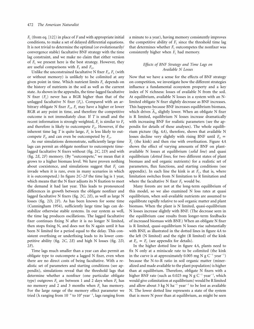
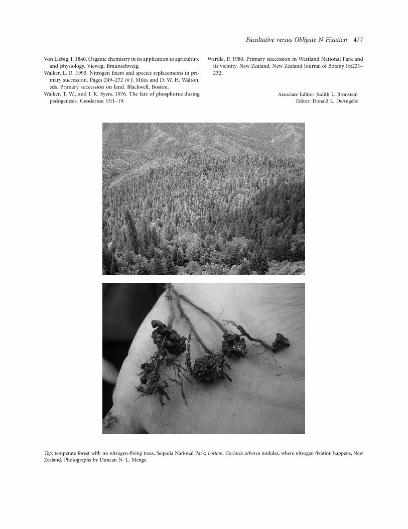
Top, temperate forest with no nitrogen-fixing trees, Sequoia National Park; bottom, Coriaria arborea nodules, where nitrogen fixation happens, NewZealand. Photographs by Duncan N. L. Menge.

1

� 2009 by The University of Chicago. All rights reserved. DOI: 10.1086/605377

Appendix from D. N. L. Menge et al., “Facultative versus ObligateNitrogen Fixation Strategies and Their Ecosystem Consequences”(Am. Nat., vol. 174, no. 4, p. 465)

Additional Calculations and Simulation DetailsParameter Values and Starting Conditions for Simulations

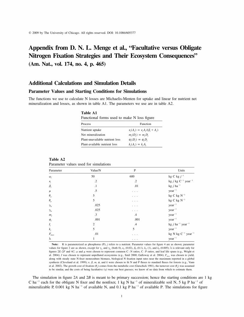
The functions we use to calculate N losses are Michaelis-Menten for uptake and linear for nutrient netmineralization and losses, as shown in table A1. The parameters we use are in table A2.

Table A1Functional forms used to make N loss figure

Process Function

Nutrient uptake n (A ) p n A /(b � A )j j j j j j

Net mineralization m (D ) p m Dj j j j

Plant-unavailable nutrient loss f (D ) p f Dj j j j

Plant-available nutrient loss k (A ) p k Aj j j j

Table A2Parameter values used for simulations

Parameter Value/N P Units

qj 50 600 kg C kg j�1

nj .2 .2 kg j kg C�1 year�1

bj .1 .01 kg j ha�1

m .5 . . . year�1

vg 5 . . . kg C kg N�1

vm 5 . . . kg C kg N�1

gg .025 . . . year�1

gm .025 . . . year�1

mj .3 .4 year�1

fj .001 .001 year�1

Ij 2 .4 kg j ha�1 year�1

kj 5 5 year�1

Fmax .01 . . . kg N kg C�1 year�1

l 1 . . . year�1

Note: R is parameterized as phosphorus (P); j refers to a nutrient. Parameter values for figure 4 are as shown; parametervalues for figure 2 are as shown, except for gg and gm (both 0), (0.02), bP (0.1), kN (1), and kP (0.005); l is relevant only fornP

figures 2E–2F and 4C; q and m were chosen to represent common C : N ratios, C : P ratios, and leaf life spans (e.g., Wright etal. 2004); I was chosen to represent unpolluted ecosystems (e.g., Smil 2000; Galloway et al. 2004); was chosen to yield,Fmax

along with steady state N-fixer monoculture biomass, biological N fixation input rates near the maximum reported in a globalsynthesis (Cleveland et al. 1999); , b, m, f, and k were chosen to fit N and P fluxes to standard fluxes for forests (e.g., Vannn

et al. 2002). The growth cost of fixation (vg) comes from the metabolic cost (Gutschick 1981), the turnover cost (vm) was assumedto be similar, and the costs of being facultative (g) were our best guesses; we know of no data from which to estimate them.

The simulation in figure 2A and 2B is meant to be primary succession; hence the starting conditions are 1 kgC ha�1 each for the obligate N fixer and the nonfixer, 1 kg N ha�1 of mineralizable soil N, 5 kg P ha�1 ofmineralizable P, 0.001 kg N ha�1 of available N, and 0.1 kg P ha�1 of available P. The simulations for figure

App. from D. N. L. Menge et al., “Facultative versus Obligate N Fixation”

2

2B–2F begin with both the facultative fixer and the nonfixer at 50%, detritus N and P at 95% and 101%, andavailable N and P at 90% and 105% of the equilibrium for the system with the facultative N fixer alone.Simulations for figure 4B and 4C are the same as for figure 2B–2F, except that the facultative N fixer begins at95% of its equilibrium biomass and the nonfixer is absent. For figure 4A, starting conditions for the equilibriumrun were the equilibrium given these functions and parameters (analytically solved by setting eqq. [1]–[5] equalto 0). For the first quasi-equilibrium run we started at the equilibrium for the N-limited nonfixer, and for thesecond we removed some plant biomass and soil organic P from the equilibrium for a slightly N-limited obligateN fixer.

Obligate Continuously Stable Strategy Calculations

To show that is a continuously stable strategy, we must show that it is both evolutionarily stable andFO

convergence stable (Eshel 1983). To show convergence stability, we must show that it will be approachedevolutionarily from any starting population at ecological equilibrium, that is, from any N-limited or R-limitedpopulation. In an equilibrium environment, N-limited N-fixing mutants Fm can invade residents Fr when

1 dBm p (q � v)(F � F ). (A1)N m rFB dt Am N,r

The quantity is the equilibrium soil-available N pool in the ecosystem with the resident alone and is aAN, r

constant. Because we have assumed that the growth benefit of N fixation (the nutrient use efficiency, qN) exceedsthe cost (v), N-limited mutants fixing more than the residents will always invade, and thus will be approachedFO

from any N-limited population. This is similar to what we found in an earlier study (Menge et al. 2008), but inthat work we examined what the costs could be and how high they would need to be.

The R-limited N-fixing mutants invade residents when

1 dBm p v(F � F ), (A2)r mFB dt Am N,r

so mutants fixing less than residents will always invade when they are R limited. Therefore, in an equilibriumenvironment, selection will push a population toward the N fixation rate that yields colimitation, so isFO

convergence stable.To show evolutionary stability, we must show that cannot be invaded once it is established. At equilibrium,FO

a population of obligate N fixers fixing at is colimited by N and R. A mutant fixing more N than theF F �O m

colimited resident (with ) would be R limited, with a lower relative growth rate (RGR) than theF F 1 F�r m r

resident:

1 dB �m p q n (A ) � vF , (A3)�R R mR, rB dt�m

1 dBr p q n (A ) � vF . (A4)R R rR, rB dtr

Because , . Conversely, a mutant fixing less N ( ) would beF 1 F (1/B )(dB /dt) 1 (1/B )(dB /dt) F F ! F� � � � �m r r r m m m m r

N limited but would still have a lower RGR than the resident:

1 dB �m p q n (A ) � (q � v)F , (A5)�N N N mN, rB dt�m

1 dBr p q n (A ) � (q � v)F . (A6)N N N rN, rB dtr

In both cases, the mutant has a lower RGR than the resident, which by definition is 0 at equilibrium, so no


3

mutants have a positive growth rate at equilibrium. Therefore, no mutant can invade , so it is evolutionarilyFO

stable and therefore a continuously stable strategy.

RGRs of FF versus Other N Fixers without Costs of Being Facultative or Time Lags

It seems intuitive that the facultative fixer FF (see eq. [9]) should always be at least as competitive as any otherN fixer as long as there is no cost to being facultative and there are no time lags. Comparing the RGRs (fromeq. [1]) of the FF with those of an arbitrary Fi proves that this intuition is right. Here, Fi can be an obligate fixer(FO), a time-lagged facultative N fixer (FL), or any N fixer other than FF, all of which would typically beoverfixing or underfixing (and therefore not colimited by N and R).

When , all plants are R limited, and Fi may pay a higher cost than FF:F ≤ 0C

1 dBF p q n (A ) � m, (A7)R R RB dtF

1 dB q n (A ) � m if F p 0i R R R ip . (A8){q n (A ) � m � vF if F 1 0B dt R R R i ii

When , all plants are N limited, and Fi may not get the same gain as FF:F ≥ FC max

1 dBF p q n (A ) � m � (q � v)F , (A9)N N N N maxB dtF

1 dB q n (A ) � m � (q � v)F if F ! Fi N N N N i i maxp . (A10){q n (A ) � m � (q � v)F if F p FB dt N N N N max i maxi

When , FF is always colimited, but Fi could be R limited or N limited:0 ! F ! FC max

1 dBF p q n (A ) � m � (q � v)F p q n (A ) � m � vF , (A11)N N N N C R R R CB dtF

1 dB q n (A ) � m � (q � v)F if F ! Fi N N N N i i Cp . (A12){q n (A ) � m � vF if F 1 FB dt R R R i i Ci

When and , and , or , the RGRs for Fi and FF are identical, butF ! 0 F p 0 F 1 F F p F F p FC i C max i max C i

everywhere else FF has a higher RGR.

Equilibrium and Quasi-Equilibrium N Loss Calculations

Equilibrium N Losses

When the plant is N limited, equilibrium available N losses are given by

m v�1k (A ) p k n � F 1 � . (A13)N N N ON { [ ( )]}q qN N

The functions kN and are monotonically increasing (assuming the inverse function exists, which it must�1 �1n nN N

for an equilibrium to exist), and , so equation (A13) shows that available N losses decrease asA q 1 vNN

biological N fixation (BNF) increases. Exploration of reasonable parameter ranges show that this decrease is verysmall relative to changes in N losses when the plant is R limited.

When the plant is R limited, equilibrium available N losses are given by the balance of inputs and the plant-unavailable N loss:

k (A ) p I � f (D ) � BF . (A14)N N N ON N


4

To determine how increasing BNF affects equilibrium losses of plant-available N, we need to know how itaffects the equilibrium values of state variables.

To do this, we first derive equilibrium expressions from equations (1)–(5), using the R-limited version ofequation (6). We leave the functions , , , and unspecified for generality, still assumingn (A ) m (D ) f (D ) k (D )j j j j j j j j

monotonicity and intersection of the origin. From setting equation (1) equal to 0,

q n (A ) p m � vF , (A15)R R OR

m � vFO�1A p n , (A16)RR ( )qR

assuming exists (which it must for to exist and therefore for the R-limited equilibrium to be biologically�1n AR R

relevant). Because is monotonically increasing, is also monotonically increasing, and therefore�1n (A ) nR R R

�AR1 0. (A17)

�FO

From setting equation (3) equal to 0,

qRB p [m (D ) � f (D )]. (A18)R RR Rm

Plugging equations (A16) and (A18) into equation (5) and setting it equal to 0,

m � vFO�1I p k n � f (D ). (A19)R R R R R( ( ))qR

Therefore,

�DR! 0, (A20)

�FO

and from equation (A18) and condition (A20),

�B! 0. (A21)

�FO

From setting equation (2) equal to 0,

mBp m (D ) � f (D ), (A22)N NN N

qN

and using condition (A21),

�DN! 0. (A23)

�FO

At equilibrium, increasing BNF when the plant is R limited decreases plant biomass ( ), soil organic N ( ),B DN

and soil organic R ( ) but increases plant-available R in the soil ( ). Therefore, the second term on the right-D AR R

hand side of equation (A14) increases with BNF, but whether the last term increases or decreases with BNFdepends on the magnitude of the change in with BNF. Specifically, the partial derivative of equilibriumBavailable N losses ( ; eq. [A14]) with respect to FO isk (A )N N


5

�k (A ) �f (D ) �B BN NN Np � � F � . (A24)O( )�F �F �F FO O O O

The first term is positive (because of monotonicity and condition [A23]), and the second depends on the sign of. If(�B/�F ) � (B/F )O O

�B B≤ , (A25)F F�F FO O

�k (A )N N1 0. (A26)

�FO

If condition (A25) is met, then a graph for the equilibrium scenario (with FO on the horizontal and onk (A )N N

the vertical) decreases until FC and then increases thereafter. For all realistic values we have tried, condition(A25) is met.

Quasi-Equilibrium N Losses

To examine how plant-available N losses depend on BNF away from equilibrium, we analyzed N losses at quasiequilibrium. In this analysis we assume that plant-available nutrients in the soil equilibrate rapidly relative toplant biomass and organic nutrients in the soil, which is generally the case in terrestrial ecosystems (see Mengeet al. 2009). Using the notation for the quasi equilibrium of AN, the effect of BNF on quasi-equilibrium lossesAN

of available N in a system with an N-limited obligate N fixer is given by

� vgˆ ˆ[k (A ) � Bn (A )] p B , (A27)N N N N ( )qN�FO

where B is treated as a constant. Because of the trade-off between BNF and N uptake from the soil, per-biomassplant uptake decreases with increasing BNF. Therefore, at the short timescale during which plant biomass iseffectively constant, N losses increase with increasing BNF. Our exploration of parameter values shows that thisis a very slight increase.

When the obligate N fixer is R limited, the effect of BNF on available N losses is greater than when it is Nlimited:

� q vR gˆ ˆk (A ) � B n (A ) p B � 1 . (A28)N N R R[ ] ( )q qN N�FO

Because , the rise in N losses when an obligate N fixer is R limited is substantially greater than whenv /q K 1g N

it is N limited. Therefore, as in the equilibrium case, BNF has little effect on plant-available N losses when theplant is N limited but a strong positive effect on N losses when the plant is R limited.

Literature Cited Only in the Appendix

Cleveland, C. C., A. R. Townsend, D. S. Schimel, H. Fisher, R. W. Howarth, L. O. Hedin, S. S. Perakis, et al.1999. Global patterns of terrestrial biological nitrogen (N2) fixation in natural ecosystems. GlobalBiogeochemical Cycles 13:623–645.

Galloway, J. N., F. J. Dentener, D. G. Capone, E. W. Boyer, R. W. Howarth, S. P. Seitzinger, G. P. Asner, et al.2004. Nitrogen cycles: past, present, and future. Biogeochemistry 70:153–226.

Gutschick, V. 1981. Evolved strategies in nitrogen acquisition by plants. American Naturalist 118:607–637.Smil, V. 2000. Phosphorus in the environment: natural flows and human interferences. Annual Review of Energy

and the Environment 25:53–88.Vann, D. R., A. Joshi, C. Perez, A. H. Johnson, J. Frizano, D. J. Zarin, and J. J. Armesto. 2002. Distribution and


6

cycling of C, N, Ca, Mg, K, and P in three pristine, old-growth forests in the Cordillera de Piuchue, Chile.Biogeochemistry 60:25–47.

Wright, I. J., P. B. Reich, M. Westoby, D. D. Ackerly, Z. Baruch, F. Bongers, J. Cavender-Bares, et al. 2004.The worldwide leaf economic spectrum. Nature 428:821–827.

Date post:	07-Sep-2018
Category:	Documents
Upload:	vunhan
View:	223 times
Download:	0 times

Facultative versus Obligate Nitrogen Fixation Strategies...

Documents