Page 1
St. Mary’s University
Faculty of Informatics
Department of Computer Science
IMPROVING ROUTING PERFORMANCE OF ROUTERS AND
CORE SWITCHES BY USING ARTIFICIALLY INTELLIGENT
NODE
By
Solomon Baye Mersha
Advisor: Dr. Asrat Mulatu
July 2019
Page 2
St. Mary‟s University
Faculty of Informatics
Department of Computer Science
A Thesis
Submitted to the Faculty of Informatics of
St. Mary‟s University
In
Partial Fulfillment of the Requirements for the Degree of Master of Science in
Computer science
IMPROVING ROUTING PERFORMANCE OF ROUTERS AND CORE
SWITCHES BY USING ARTIFICIALLY INTELLIGENT NODE
By
Solomon Baye Mersha
Advisor: Dr. Asrat Mulatu
July 2019
Page 3
St. Mary‟s University
Faculty of Informatics
Department of Computer Science
IMPROVING ROUTING PERFORMANCE OF ROUTERS AND CORE
SWITCHES BY USING ARTIFICIALLY INTELLIGENT NODE
By
Solomon Baye Mersha
APPROVAL BY BOARD OF EXAMINERS
_______________________ __________________________
Chairman Department of Graduate Signature
________________________ __________________________
Advisor Signature
________________________ __________________________
Examiner Signature
________________________ __________________________
External Examiner Signature
Page 4
DECLARATION
I, the undersigned, declare that this thesis work is my original work, has not
been presented for a degree in this or any other universities, and all sources of
materials used for the thesis work have been duly acknowledged.
Solomon Baye Mersha ______________________________________
Full Name of Student
_________________________________
Signature
Addis Ababa
Ethiopia
This thesis has been submitted for examination with my approval as advisor.
Dr. Asrat Mulatu __________________________________
Full Name of Advisor
________________________________
Signature
Addis Ababa
Ethiopia
July, 2019
Page 5
i
Acknowledgements
First and foremost, I would like to thank God without whose assistance nothing would have
been successful.
I would like to express my deepest gratitude to my advisor, Dr. Asrat, for his motivational
and constructive guidance right from the moment of problem formulation to the completion
of the work. Many thanks and an appreciation goes to him for his excellent guidance,
supervision and advice during the course of this thesis. His valuable advices in conducting
scientific research, discussions with him always made me think that things are possible. His
enthusiasm and encouragement has always inspired me to accelerate to the completion of the
work.
Finally, I like to express my deepest gratitude to my parents for being a constant source of
loving support, patient, and encouragement throughout the year. My special thanks goes to
my beloved brother Professor Tesfaye Baye for your encouragement and financial support in
all my endeavors.
Solomon Baye
Page 6
ii
Abstract
A routing protocol is plays an important role in today‟s communication networks. It is also a
protocol which is in charge of determining how routers and core-switches interconnect with
each other and forward the packets through the best path to travel from a source to a
destination using a predefined and user defined path finding and search algorithms. The
leading and well-known routing protocols are Enhanced Interior Gateway Routing Protocol
(EIGRP) and Open Shortest Path First (OSPF).In the metrics of Internet routing protocol
performance, each of them has different architecture, flexibility, route processing delays and
convergence abilities. The A* search algorithm is the more optimal and complete search
algorithm than that of Dijkstra algorithm and perfect for finding the shortest path. This thesis
presents a simulation-based combination of Enhanced Interior Gateway Routing Protocol
(EIGRP) and A* search algorithm by using Network Simulator 2 (NS2). For performance
evaluation of this combination, two network models are designed and configured with EIGRP
and EIGRP with A* search algorithms. The evaluation of the proposed routing protocol is
performed based on the quantitative metrics such as delay, throughput and packet loss through
the simulated network models. The evaluation results show that EIGRP routing protocol with
A* search algorithm provides better performance than EIGRP routing protocol.
Keywords: EIGRP, OSPF, A* star, NS2, intelligent node.
Page 7
Table of Contents
Acknowledgements ..................................................................................................................... i
Abstract ......................................................................................................................................ii
List of Figures .......................................................................................................................... iii
List of Tables ...........................................................................................................................IV
List of Abbreviations ................................................................................................................ V
CHAPTER ONE: INTRODUCTION ........................................................................................ 1
1.1 Background ................................................................................................................. 1
1.2 Motivation ................................................................................................................... 4
1.3 Statement of the Problem ............................................................................................ 5
1.4 Objectives of the Research .......................................................................................... 6
1.4.1 General objective ................................................................................................. 6
1.4.2 Specific objectives ............................................................................................... 6
1.5 Methodology ............................................................................................................... 6
1.6 Research Questions ..................................................................................................... 7
1.7 Scope and Limitation .................................................................................................. 7
1.8 Organization of the thesis ............................................................................................ 7
CHAPTER TWO: LITRATURE REVIEW .............................................................................. 8
2.1 Technical Overview of Routing Protocols .................................................................. 8
2.1.1 General Overview ................................................................................................ 8
2.1.2 Features of Routing Protocols ............................................................................ 12
2.1.3 Parameters of Routing........................................................................................ 12
2.1.4 Types of Routing Protocols ............................................................................... 13
2.1.5 Static versus Dynamic Routing .......................................................................... 14
2.1.6 Class-full and Classless Routing Protocols........................................................ 14
2.1.7 Link State Routing ............................................................................................. 16
2.1.7.1 Features of LSR .............................................................................................. 17
2.1.7.2 Techniques of Routing ................................................................................... 17
2.1.7.3 Advantages and Disadvantages of LSR ......................................................... 17
2.1.8 Distance Vector Routing .................................................................................... 17
2.2 The A star (*) search algorithm in Artificial Intelligence ......................................... 19
2.2.1 Heuristic Functions ............................................................................................ 21
2.2.2 Admissible Heuristics ........................................................................................ 22
2.2.3 Consistent Heuristics ......................................................................................... 23
2.2.4 Performance of A*search algorithm .................................................................. 23
Page 8
2.2.5 Pseudo code for A* ............................................................................................ 25
CHAPTER THREE: RELATED WORKS .............................................................................. 28
3.1 Related to Artificial Intelligent ................................................................................. 28
3.2 Related to Routing protocols ..................................................................................... 30
3.3 Research Gaps ........................................................................................................... 30
CHAPTER FOUR: ENHANCED INTERIOR GATEWAY ROUTING PROTOCOL .......... 31
4.1 Introduction ............................................................................................................... 31
4.2 Protocol Structure ...................................................................................................... 31
4.3 Technique of EIGRP ................................................................................................. 33
4.3.1 Neighbor Discovery/Recovery........................................................................... 33
4.3.2 Reliable Transport Protocol ............................................................................... 34
4.3.3 Diffusion Update Algorithm .............................................................................. 34
4.4 EIGRP Metrics .......................................................................................................... 37
4.5 EIGRP Convergence ................................................................................................. 38
CHATER FIVE40: RESULTS AND DISCUSSIONS ............................................................ 40
5.1 Introduction ............................................................................................................... 40
5.2 Structure of NS-2 ...................................................................................................... 40
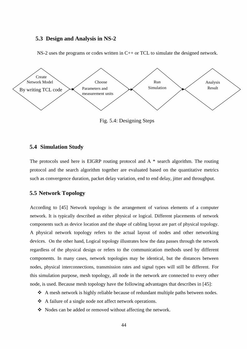
5.3 Design and Analysis in NS-2 .................................................................................... 44
5.4 Simulation Study ....................................................................................................... 44
5.5 Network Topology .................................................................................................... 44
5.6 Measurements............................................................................................................ 47
5.7 Simulation Results and Analysis ............................................................................... 47
CHAPTER SIX52: CONCLUSIONS AND FUTURE WORKS............................................. 52
References ................................................................................................................................ 53
Annex A: Sample source code for the topology used. ............................................................. 56
Page 9
iii
List of Figures
FIG. 2.1: CLASS-FULL ROUTING WITH SAME SUBNET MASK ........................................................ 15
FIG. 2.2: CLASSLESS ROUTING WITH DIFFERENT SUBNET MASK.................................................. 16
FIG. 4.1: DUAL PLACED IN THE NETWORK .................................................................................. 36
FIG. 4.2: FAILURE LINK OF NETWORK TOPOLOGY ....................................................................... 37
FIG. 4.3: FAILURE LINK OF NETWORK TOPOLOGY ....................................................................... 37
FIG. 4.4: NETWORK TOPOLOGY OF EIGRP .................................................................................. 39
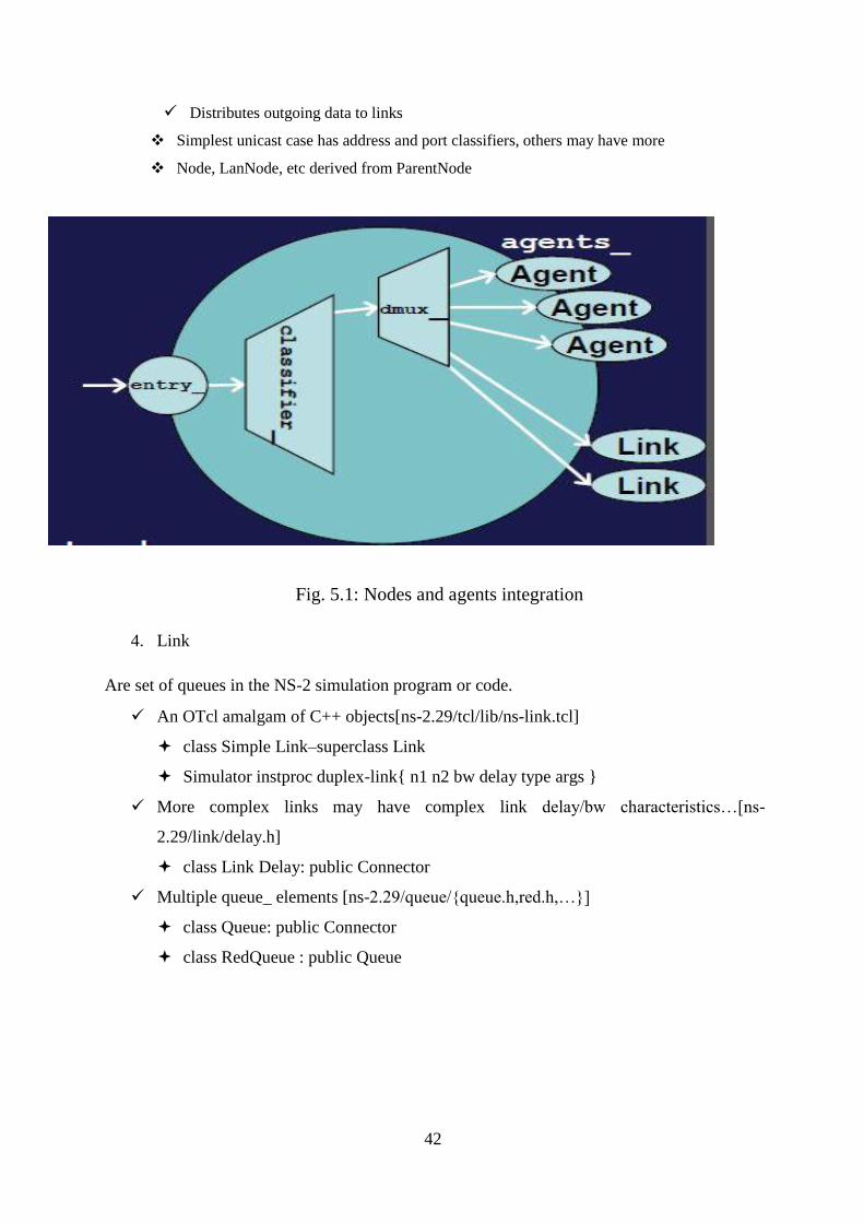
FIG. 5.1: NODES AND AGENTS INTEGRATION .............................................................................. 42
FIG. 5.2: LINK EXAMPLE AND SOME FUNCTIONS IN IT ................................................................. 43
FIG. 5.3: ARCHITECTURE OF NS-2 ............................................................................................... 43
FIG. 5.4: DESIGNING STEPS......................................................................................................... 44
FIG. 5.5: WIRED NETWORK TOPOLOGY WITH 12 NODES .............................................................. 45
FIG. 5.7: WIRED NETWORK TOPOLOGY COMMUNICATION LINE FAILURE .................................... 46
FIG. 5.8: THROUGHPUT OVER EIGRP AND EIGRP WITH A* SEARCH ALGORITHM .......................... 49
FIG. 5.9: PACKET LOSS OVER EIGRP AND EIGRP WITH A* SEARCH ALGORITHM ........................... 50
FIG. 5.10: DELAY OVER EIGRP AND EIGRP WITH A* SEARCH ALGORITHM ................................... 51
Page 10
iv
List of Tables
TABLE 2.1: COMPARISONS OF PROGRAMMING WITHOUT AND WITH AI ..................................... 11
TABLE 2.2: CLASSIFICATION OF ROUTING PROTOCOLS ............................................................. 14
TABLE 4.1: PROTOCOL STRUCTURE OF EIGRP ......................................................................... 31
TABLE 4.2: EIGRP INTERVAL TIME FOR HELLO AND HOLD ...................................................... 34
TABLE 5.1: SIMULATION RESULTS ............................................................................................ 47
Page 11
V
List of Abbreviations
ABR Area Border Router
ADSL Asymmetric Digital Subscriber Line
AI Artificial Intelligence
App Application
BDR Backup Designated Router
BGP Border Gateway Protocol
CBR Constant bit rate
CIDR Classless Inter Domain Routing
CPU Central Processing Unit
DES Discrete Event Simulation
DR Designated Router
DUAL Diffusion Update Algorithm
EIGRP Enhanced Interior Gateway Routing Protocol
IP Internet Protocol
ISP Internet Service Provider
LAN Local area Network
LSA Link-State Advertisement
LSAck Link-State Acknowledgement
LSDB Link-State Database
LSP Link State Packet
LSR Link-State Request
LSU Link-State Update
MAC Media Access Control
NAM Network Animator
NET Network Entity Title
NS2 Network Simulator 2
NSAP Network Service Access Point
NSSA Not-So-Stubby-Area
OPNET Optimized Network Engineering Tool
OSI Open Systems Interconnection
OSPF Open Shortest Path First
OTCL Object-Oriented Tool Command Language
PSNP Partial Sequence Number Packet
RAM Random Access Memory
RD Reported Distance
ROM Read Only Memory
VRAM Volatile Radom Access Memory
WAN Wide Area Network
Page 12
1
CHAPTER ONE
INTRODUCTION
1.1 Background
Because of the wide advancement in technology and need for communication, there is a great
demand for network communication. The mechanism and management of this communication
takes-off with interaction among networks which is performed with the help of Routing.
Routing protocol helps as a basis for communication among different users in huge computer
networks [1] Presently, these protocols are on in wide-ranging use, Like OSPF, RIP, EIGRP,
and BGP are practical using the routing table‟s information available with each node in the
network. Routing protocols play a remarkable role for forwarding or to route the user data to
its right destination. The job of routing protocols is very critical in terms of choosing the right
route for user traffic and to forward it by having various networks limitations. There are
number of routing protocols that have developed such as OSPF (Open Shortest Path First),
RIP (Routing Information Protocol) and EIGRP (Enhanced Interior Gateway Routing
Protocol) [2], [3] , [4]. All these mentioned protocols are based on their own routing process
and thus does convergence with any topological change in the network. According to [2], [4]
routing process can be defined as to select the best path among multiple paths from where the
user data can be forwarded towards its destination. Most routing protocols are used to fix the
shortest path from the sender to the receiver. Thus, each routing protocol has different routing
process from the other. Therefore, the performance of each routing protocol differs when
applying to the network having some real type of network limitations. Differences in network
are the result of the change in traffic patterns, accessibility of new network resources and of
removal, or failure of network resources.
For network optimization, routing protocols have got an important part of moving the user
traffic across the network without compromising the network resources. For this purpose,
routing process is performed by the routers in the network which uses any of the mentioned
routing protocols. It should be noted here that OSPF, RIP and EIGRP use their own routing
process which is different from the other [2]. This divergent approach makes each routing
protocol special from the other and thus every protocol performs in a different manner with
various network situations.
Page 13
2
Open Shortest Path First (OSPF), Enhanced Interior Gateway Routing Protocol
(EIGRP),Routing Information Protocol and Intermediate System to Intermediate System (IS-
IS) are the leading interior routing protocols for such networks [5].
Enhanced Interior Gateway Routing Protocol (EIGRP) is an enhanced version of Interior
Gateway Routing Protocol (IGRP) was introduced by Cisco in 1993 named as Enhanced
Interior Gateway Routing Protocol (EIGRP) [6]. It is a distance vector routing protocol that
uses an algorithm called as DUAL (Diffusion Update Algorithm). However, it is considered
as hybrid routing protocol because it has also got the properties of link state protocols [2].
Hence, this routing protocol contains the features of both link state and distance vector routing
protocols. EIGRP protocol is mostly used for large networks. Any router in the network which
uses EIGRP protocol it keeps all routes in its routing table. This routing protocol also does
convergence when there is any topological change occur in the network [3]. EIGRP protocol
operation is based on four components such as Neighbor Discovery/ Recovery, Reliable
Transport Protocol (RTP), DUAL and Protocol dependent module [7]. Neighbor discovery is
one of the processes of EIGRP protocol in which a router discovers its neighbor routers by
sending HELLO packets with regular interval of time. RTP ensures the reliable transmission
of unicast or multicast packets of EIGRP protocol in the network [7]. DUAL plays a major
role as a loop avoidance mechanism which is used for the topological change in the network.
Open Shortest Path First (OSPF) Routing Protocol For IP networks, Internet Engineering Task
force introduced a link state routing protocol in mid-80`s named Open Shortest Path First
(OSPF) routing protocol. OSPF widely uses in large enterprise networks because of its
efficient convergence in the network [7]. Any dynamic routing protocol, routers distribute
network topology information across the network. This exchange of topology information
among the routers of the network is called as convergence activity. And the time spent for this
activity is considered as convergence duration of the routing protocol [8], [9]. As OSPF is a
dynamic routing protocol, so all routers that are configured with OSPF protocol will exchange
the link state routing information to all the connected routers and thus build their own routing
table. The routing table in each router is based on information it received from the other
routers. Having routing table in each router, the Dijkstra algorithm is used to find the shortest
route from the current router to all the connected routers [7]. When any link fails/ set
(recovered) in the network, then all the routers in the network become active and therefore do
convergence activity. During this convergence activity, each router exchanges this topological
Page 14
3
change (link fails/ set) information across the network. And once each router is updated with
the latest change in the network, it again updates its routing table [2], [3], [7].
RIP (Routing Information Protocol) is considered as one of the major distance vector routing
protocol which offers hop count as a routing metric. It is an interior gateway routing protocol
which works within an autonomous network system [8]. Typical RIP routing protocol offers a
maximum of 15 hops count from sources towards the destination and therefore provide loop-
free routing. Limitation of 15 hops count makes RIP routing protocol for the limited size
network. Thus, offering more than 15 hops count destination as unreachable from source in
RIP configured routing protocol [8], [10]. In RIP configured network, routers send and
receive Request Message and Response Message from other RIP configured routers in the
network with regular interval of time. This protocol uses set of timers as an important part for
its convergence activity. These timers are named as update timer, invalid timer, flush timer
and hold-down timer [8], [10]. Therefore, when the network is configured with RIP, this
protocol is considered as a routing protocol that has slow convergence activity with limited
hop counts but has less CPU utilization in the network. However, RIP can behave differently
in terms of topological change from other two (OSPF and EIGRP) routing protocols as it
converges in a different process.
EIGRP is a vendor specific that is industrialized by the company called Cisco. It is distance-
vector protocol based on Diffusing Update Algorithm (DUAL). EIGRP is the only routing
protocol that has got characteristics of both link state and distance vector routing Protocols.
Nevertheless, the convergence time of EIGRP is faster than other protocols. It is also easy to
configure. In other ways, OSPF is a link-state interior gateway protocol based on Dijkstra
algorithm. OSPF routing protocol needs more time and knowledge to configure network and
with high memory requirements.
The key and important functionality of routing protocols in IP networks is to carry data
packets and sent them from sender to receiver. Transmitting data from a sender to a receiver
by hopping one-node or multi-node is called routing. Routing protocols provide two facilities:
firstly choosing paths for different pairs of sender/receiver nodes and, effectively transmitting
data to the receiver.
Routing protocols are used to describe how routers and core switches communicate to each
other, build routing tables information, make routing decisions and share information among
neighbors. Routers and core switches are used to connect multiple different networks and to
Page 15
4
provide packet forwarding for different types of networks. The main goal of routing protocols
is to discover the optimum and best path from a sender to a receiver. These routing algorithms
use different parameters based on a single or on several properties of the path in order to
determine the optimal way to reach a given network.
Generally, routing protocol is the language a router speaks with other routers in order to share
information about the reachability and status of network. It includes a procedure to select the
best path based on the reachability information it has and for recording this information in a
route table. Regarding to select the best path, a routing metric will be applied and it is
computed by a routing algorithm. And routing protocol is taking an important and non-
changeable role in today‟s communication networks. Protocols are also equipped with a
procedure which is accountable for determining how routers communicate with each other and
forward the packets through the best path to travel from a sender node to a receiver node.
1.2 Motivation
Every network especially IP-based networks need a more secure, robust and effective routing
protocol for fast convergence, short end to end delay and the ability to recover from
emergencies quickly [11]. The main motivation behind this is that to discover and open a
begging solution for best performance of routing protocols by combining artificial intelligence
search algorithms. Secondly, to analyze and show that artificial intelligence can be integrated
with routing protocols so that an artificial intelligent node can be used to improve the routing
performance of routers and core switches. Thirdly, find out the best routing protocols from the
existing one and selecting search algorithms from AI.
Routing protocol performance can be measured by convergence times which are aimed and as
a performance metrics for real-time applications are delay variation, end to end delay, jitter
and throughput.
Simulation and validation are carried out by using NS2, GNS3, OPNET, JAVA and other
simulation software‟s.
Page 16
5
1.3 Statement of the Problem
There are many problems and obstacles that reduce and minimize the routing
performance of routers and core-switches. So, these problems are the following.
1. Routers and core-switches use already configured routing protocol to determine the best
and optimal path where that stored configuration might be corrupt, lost, damaged or
malfunction and let the network fail.
2. Each router and core-switch participating in the network must know something about
global state where this global state is
Inherently large
Dynamic
Hard to collect
This leads to problem in decision making (for both local and global) one.
3. A routing protocol must intelligently summarize relevant information about the network
to minimize the routing table space. This helps the routing table to be
fast to look up
less to exchange
This improves the bandwidth optimization and performance of the routing protocols
and, generally the network itself.
4. Routers and core-switches in the network must minimize number and frequency of
control messages to achieve a better and effective performance in all metrics of quality
of service. This scenario leads the network to be robust and this can help to avoid
black holes
loops
oscillations
Therefore, the above problems and concepts of routing motivated me to do research on
routing protocols with the composition of artificial intelligence.
Page 17
6
1.4 Objectives of the Research
1.4.1 General objective
The general objective of this research is to compare an effective routing algorithm by
introducing artificial node in the network and using the concepts of A* search algorithm with
respect to routing protocol.
1.4.2 Specific objectives
The specific objective of this research is listed below.
To analyze and select best routing protocol from the existing protocols
Finding out the best search algorithms in artificial intelligence in respect to routing
protocols that can suit for it and selecting one.
The selected search algorithm and routing protocol will be used to define an artificial node
According to the selected routing protocol and search algorithms combined together in a
compatible way to produce a best solution for the stated problems in the routing protocols.
1.5 Methodology
The following different kinds of methods and techniques are used in this thesis. By literature
review, different kinds of papers on routing and A * search algorithm has been studied
extensively and in- depth analysis is made on the following main concepts.
What is routing protocols and which one is the best routing protocol among them.
Routing protocol in detail analysis
Search algorithms and their comparison among the different search algorithms in an
artificial intelligence searches.
A * search algorithm and its main idea and concept in respect to other search
mechanisms.
Ant colony optimization and their essence for routing
Simulation based comparison of routing protocols.
Different simulation and emulation software studied in detail.
Applications of neural network in routing
Designing a new protocol by combining EIGRP and A* search algorithm.
Collect and analyses the result.
Validate the result or comparatively analyses the result.
Page 18
7
1.6 Research Questions
The following are the main research questions addressed in this research
Which routing protocol or algorithm is best from the currently used once?
What search algorithm in artificial intelligence will suit for routing?
How to develop best solution for routing performance by combining search
algorithm and routing algorithm?
1.7 Scope and Limitation
This research work only focus studying about the routing protocols and identifying one from
an existing one and then select best and suitable search algorithm for the selected routing
protocol. Thus, the selected search algorithm with the combination of the routing protocol
helps to improve the performance of routing protocols in routers and core-switches by
introducing an artificial node.
In doing this thesis there are limitations and difficulties that challenges me. These limitations
include finding out an outline for doing this thesis paper, software were not that much
accessible and almost commercial one. Due to this reason it was difficult to find out the right
software for the simulation and even though it was not possible to purchase it from outside
due to the lack of credit card that can work outside our country. The other one is shortage of
time, in accessible resources and hardware constraint.
1.8 Organization of the thesis
This thesis report is composed of six chapters. In the second chapter literature review in-depth
study of routing protocols and techniques is described with suitable examples and graphs and
about the Artificial Intelligence search namely A * star search algorithm in detail and shows
that how it will suit for the selected routing protocol i.e. EIGRP. The third chapter is discusses
about related work. The fourth chapter discusses about the selected routing protocol for this
thesis which is namely Enhanced Interior Gateway Routing Protocol (EIGRP) in detail and
with respect to the other routing protocols existed today. The fifth chapter is about the tools
and techniques used to do this thesis paper and the simulation and emulation software used.
Finally, the research findings and recommendations are presented in chapter six.
Page 19
8
CHAPTER TWO
LITRATURE REVIEW
2.1 Technical Overview of Routing Protocols
2.1.1 General Overview
Routing protocol has a significant role in today‟s network and communication technologies
improvement and growth by providing effective services. A routing protocol transports
packets by transferring them between different nodes in different and many networks. When
bearing in mind of a network, routing takes place (node or hop by node or hop). So, routing
protocols have the following objectives: To communicate between routers and core-switches,
to build routing tables information‟s among the neighboring node and the whole network, to
make precise and simple routing decisions, to learn existing routes (learning from the existing
information) and to share information amongst neighboring routers and core-switches.
The routers and core-switches are used mostly by connecting several networks and providing
packet forwarding to different networks. The main point for routing protocols is to establish
the best path from the source to the destination. A routing algorithm services several metrics,
which are used to resolve the best method of reaching to a given network. These are
established either on a single or on several properties of the path. Link State Routing
Protocols and Distance Vector Routing Protocols are some classifications of routing
protocols. This routing protocol is usually used for other types of communication networks
such as Wireless Ad-Hoc Networks, Wireless Mesh Networks and so on.
Routers
A router is a computer networking device that forwards data packets towards their
destinations through a process called routing. Router operates network layer of OSI model.
The Internal components of routers are Central Processing Unit (CPU), Random Access
Memory (RAM), Non Volatile Radom Access Memory (NVRAM), Flash and Read Only
Memory (ROM).Routers have at least two network interfaces. These are LAN Interface and
WAN interface. LAN Interfaces used to connect router to LAN network. It has a layer 2
MAC address and can be assigned a Layer 3 IP address and usually consist of an RJ-45 jack.
WAN Interfaces are used to connect routers to external networks that interconnected LANs.
Depending on the WAN technology, layer 2 address may be used. It uses a layer 3 IP address.
Page 20
9
According to the features and applications, routers are divided into four major categories.
Broadband Routers: Broadband routers are used to connect computers/Laptops to connect to
the Internet. Broadband routers are required when we connect internet through phones. ADSL
modems are used for this purpose as they embed both phone and Ethernet jacks.
Wired and Wireless Routers: These days wired and wireless routers are most commonly
used in the home and small office networking. Wired and wireless routers are able to transmit
internet signals and maintain routing information in their routing table. They are also capable
to filter traffic on IP addresses base.
Edge Router: Edge routers are placed at the edge of the ISP network. These are normally
configured to external routing protocols like BGP (Border gateway protocol) and OSPF (Open
Shortest Path First) to another BGP or OSFP of other ISP or large organization.
Core Router: Core router is used as the backbone of the LAN network. In some deployment
scenarios, a core router may perform as a step-down backbone that interconnects the
distribution routers from different branches of an organization. These routers possess high
performance capabilities.
Core Switches
A core switch is a high capacity switch generally positioned within the backbone or physical
core of networks. Core switch serves as the gateway to wide area network (WAN) or the
Internet. As the name implies, a core switch is central to the network and needs to have
significant capacity to handle the load sent to it. They provide the final aggregation point for
the network and allow multiple aggregation modules to work together. In a public WAN, a
core switch interconnection edges switch that are positioned on the edge of related network.
In a local area network (LAN), this switch interconnects work group switch, which are
relatively low capacity switch that are usually positioned in geographic clusters.
The difference between Core switch and other switch is:
Core switch is required to always be fast, highly available and fault tolerant since it
connects the entire aggregation switch. Therefore, a core switch should be a fully
managed switch. But if it is a switch not used in the core layer, it can be smart switch
or an unmanaged switch.
Page 21
10
Core switch is not always needed in a LAN while we may often have the aggregation
switch and the access switch. Because in small networks that have only a couple so
servers and a few client, there is no actual demand for a core switch vs aggregation
switch.
Only one core switch used in a small or midsize network, but the aggregation layers
and the access layers might have multiple switches.
Switches are different from routers because routers operate at the Network layer (Layer 3) of
the OSI model while switches operate at the Data Link layer (Layer 2). Routers use IP
addresses to forward traffic, while switches use MAC addresses for this purpose. A MAC
address is permanently configured on network adapters by their manufacturers and cannot be
changed. Some Layer 3 switches operate at the Network layer of the OSI model.
Switches offer better security to networks because they use MAC addresses and can filter out
traffic coming in from an unknown MAC address. Switches are better than hubs because they
forward only incoming packets to the desired destination instead of broadcasting them to all
devices.
Artificial Intelligent (AI) Overview
According [12] to the father of Artificial Intelligence, John McCarthy, it is “The science and
engineering of making intelligent machines, especially intelligent computer programs”.
Artificial Intelligence is a way of making a computer, a computer-controlled robot, or a
software think intelligently, in the similar manner the intelligent humans think.
AI is accomplished by studying how human brain works and how humans learn, decide, and
work while trying to solve a problem, and then using the outcomes of this study as a basis of
developing intelligent software and systems.
The Goals of AI describes in is [12]:
To Create Expert Systems: The systems which exhibit intelligent behavior, learn,
demonstrate, explain, and advice its users.
To Implement Human Intelligence in Machines: Creating systems that understand,
think, learn, and behave like humans.
Page 22
11
Artificial intelligence contributes to science and technology based on disciplines such as
Computer Science, Biology, Psychology, Linguistics, Mathematics, and Engineering. A
major thrust of AI is in the development of computer functions associated with human
intelligence, such as reasoning, learning, and problem solving. The programming without and
with AI is different in the following ways. Table 2.1 shows the comparison of the two.
1Table 2.1: Comparisons of Programming without and with AI
Programming Without AI
Programming Within AI
A computer program without AI can answer
the specific questions it is meant to solve.
A computer program with AI can answer
the generic questions it is meant to solve.
Modification is not quick and easy. It may
lead to affecting the program adversely.
Quick and Easy program modification.
Modification in the program leads to change
in its structure.
AI programs can absorb new modifications by
putting highly independent pieces of
information together.
Applications of AI
There are many important applications of AI. The following are most ultimate usages of
AI [12].
Gaming: AI plays crucial role in strategic games such as chess, poker, tic-tac-toe,
etc., where machine can think of large number of possible positions based on
heuristic knowledge.
Natural Language Processing: It is possible to interact with the computer that
understands natural language spoken by humans.
Expert Systems: There are some applications which integrate machine, software, and
special information to impart reasoning and advising. They provide explanation and
advice to the users.
Vision Systems: These systems understand, interpret, and comprehend visual input on
the computer. For example,
Page 23
12
Speech Recognition: Some intelligent systems are capable of hearing and
comprehending the language in terms of sentences and their meanings while a human
talks to it. It can handle different accents, slang words, noise in the background,
change in human‟s noise due to cold, etc.
Handwriting Recognition: The handwriting recognition software reads the text
written on paper by a pen or on screen by a stylus. It can recognize the shapes of the
letters and convert it into editable text.
Intelligent Robots: Robots are able to perform the tasks given by a human. They
have sensors to detect physical data from the real world such as light, heat,
temperature, movement, sound, bump, and pressure. They have efficient processors,
multiple sensors and huge memory, to exhibit intelligence. In addition, they are
capable of learning from their mistakes and they can adapt to the new environment.
2.1.2 Features of Routing Protocols
The features of routing protocols are:
Convergence:
The time required for all routers in the network should be small so that the routing
specific information can be easily known.
Loop Free:
The routing protocol of router and core-switches should ensure a loop free route. The
benefit of using, such routes are to efficiently obtain the available bandwidth.
Best Routes:
The routing protocol selects the best path to the destination network.
Security:
The protocol ensures a secured transmission of the data to a given destination.
2.1.3 Parameters of Routing
2.1.3.1 Parameters
The measurement path cost usually depends on metric parameters. Metrics are used in a
routing protocol to decide which path to use to transmit a packet through an internetwork.
Page 24
13
2.1.3.2 Purpose of a Metric
A value applied by the routing protocols, namely metric, is used to allocate a cost for reaching
the destination. Metrics fix the optimal and best path in case of multiple paths present in the
same destination by allocating the cost and evaluate the optimal path. Analyzing the metrics
has many different ways for each routing protocols. For example, OSPF uses bandwidth while
RIP (Routing Information Protocol) uses hop count and EIGRP uses a combination of
bandwidth and delay.
2.1.3.3 Metric Parameters
The ranking of routes from most preferred to least preferred is measured by a metric.
Different metrics are used by different routing protocols. In IP routing protocols, the
following metrics are used mostly [13].
Hop count: It counts the number of routers for which a packet traverses in order to
reach the destination.
Bandwidth: A bandwidth metric chooses its path based on bandwidth speed thus
preferring high bandwidth link over low bandwidth.
Delay: Delay is a measure of the time for a packet to pass through a path. Delay
depends on some factors, such as link bandwidth, utilization, physical distance
traveled and port queues.
Cost: The cost can be represented either as a metric or a combination of metrics. The
network administrator can estimate the cost to specify an ideal route.
Load: It is described as the traffic utilization of a defined link. The routing protocol
use load in the calculation of a best route.
Reliability: It computes the link failure probability and it can be calculated from
earlier failures or interface error count.
2.1.4 Types of Routing Protocols
The following list presents the mostly used classifications of routing protocols:
Static and dynamic routing protocols.
Distance Vector and Link State routing protocols.
Class-full and Classless routing protocols.
Page 25
14
2.1.5 Static versus Dynamic Routing
A routing process that a routing table follows a manual construction and fixed routes at boot
time is called Static routing. This routing table information should be updated by the device
and even by the network administrator when a new network is added and discarded in the
network. For small network Static routing is suitable. Its performance degrades when the
network topology is changed. The network administrator usually uses this information for
controlling and maintaining the whole network.
The network has more control over the network in static routing. Its simple functionality and
less CPU processing time are also advantages. The disadvantages of static routing are poor
performance experienced when network topology changes, complexity of reconfiguring
network topology changes and difficult manual setup procedure.
On the other hand, dynamic routing is a routing protocol in which the routing tables are
formed automatically by using the routing protocol configuration such that the neighboring
routers and core-switches exchange messages with each other. The optimal and best path
procedure is piloted on the basis of bandwidth, link cost, hop number and delay. The protocol
usually updates these values. Dynamic routing protocol has the advantage of shorter time
spent by the administrator in maintaining and configuring routes. However it has variety of
problems like routing loops and route inconsistency.
2.1.6 Class-full and Classless Routing Protocols
Based on the subnet mask, routing protocols are divided into Class-full and Classless routing
as below:
2Table 2.2: Classification of Routing Protocols
Distance Vector Link State Class
IGRP, RIP Class-full
RIPv2, EIGRP OSPF, IS-IS, NLSP Classless
Page 26
15
2.1.6.1 Class-full Routing
In Class-full routing, subnet masks achieve the same functionality all through the network
topology and this kind of protocol does not send information of the subnet mask. A router
makes the following functions and services to calculate a route [13], [14]. Routers use the
same subnet mask which is directly connected to the interface of the major network. When the
router is not directly connected to the interface of the same major network, it applies Class-
full subnet mask to the route.
Class-full routing protocols are not used widely because:
It cannot include routing updates.
It cannot be used in sub-netted networks.
It is not able to support Variable Length Subnet Masks (VLSM).
It is unable to support dis-contiguous networks.
.
Fig. 2.1 is an example of a network where Class-full routing is used with the same subnet
mask all through the network.
1Fig. 2.1: Class-full routing with same subnet mask [13].
2.1.6.2 Classless Routing
In classless routing the subnet mask can be changed in the network topology and routing
updates are included. Most networks do not depend on classes for being allocated these days
Page 27
16
and also for determining the subnet mask, the value of the first octet is not used. Classless
routing protocols support non end-to-end networks [13].
2Fig. 2.2: Classless routing with different subnet mask [13].
2.1.7 Link State Routing
The Link State Routing (LSR) includes the Shortest Path First (SPF) where the functions and
capabilities of routers and core-switches are to determine the shortest path among the network
and store the information (The routing table information) in a database called link state
database.
Switching the routing information among the nodes is done by the Link State Advertisements
(LSA). By using flooding the information of the neighbors found in each LSA of a node and
any change in link information of a neighbor‟s node is communicated through LSAs. When
LSAs are received the nodes will observe the change. Then the routes are calculated again and
resent to their neighbors. Finally, all nodes can maintain an identical database where they
describe the topology of the networks. These link state or routing table information databases
provide information of the link cost in the network and then a routing table is formed. This
routing table carries information about the forwarded packets and also indicates the set of
paths and their link cost. For calculating the path and cost for each link
Dijkstra algorithm is used. The link cost is set by the network operator which is the bandwidth
and the network line, represented as the weight or length of that particular link.
After the link cost is assigned load balancing performance is achieved. Then the network
congestion can be avoided. Thus, a network operator can change the routing by varying the
link cost. Generally, the weights are left with the default values and it is suggested to inverse
the link‟s capacity and then assigns the weight of a link on it. However, LSR protocols have
Page 28
17
better flexibility. Link state protocols make better routing decision and minimize overall
broadcast traffic and are able to make a better routing decision.
Two of the most common types of LSR protocols are OSPF and IS-IS. OSPF determines the
shortest distance between nodes based on the weight of the link.
2.1.7.1 Features of LSR
The features of LSR are: Each router keeps the same database, large networks
split into sub areas, include multiple paths to destination, faster non loop
convergence and support an accurate metrics.
2.1.7.2 Techniques of Routing
Each router is responsible for accomplishing the following process [13].
Each router learns about directly connected networks and its own links.
Each router must have a connection with its directly connected adjacent networks and
this is usually performed through HELLO packet exchanges.
Each router must send link state packets which contains the state of the links.
Each router stores a link state packet copy which is received by its neighbors.
Each router independently establishes the least cost path for the topology.
2.1.7.3 Advantages and Disadvantages of LSR
Routers calculate routes independently and are independent of the calculation of intermediate
routers in LSR protocols [15].
The major advantages of link state routing protocols are: They react very fast to change in
connectivity and the packet size is very small. Disadvantages of link state routing are: Huge
memory requirements, more complex to configure and ineffective under mobility for link
changes.
2.1.8 Distance Vector Routing
In Distance vector routing protocol routes are function of distance and direction vectors where
the distance is represented as hop count metrics and direction is represented as exit interface.
The Bellman Ford algorithm is mainly used for the path calculation where the nodes take the
Page 29
18
position of the vertices and the links in DVR. So in DVR, for each destination, a specific
distance vector is maintained for all the nodes used in the network. The distance vector
includes of destination ID, shortest distance and next hop. In this routing each node passes a
distance vector to its neighbor and informs about the shortest paths. Every node depends on its
neighboring nodes for collecting the route information.
Thus they discover routes coming from the adjacent nodes and advertise those routes
information from their own side. Those nodes are responsible for exchanging the distance
vector and the time needed for this purpose can vary from 10 to 90 seconds. When a node in a
network path accepts the advertisement of the lowest cost from its neighbors, the receiving
node then adds this entry to the routing table.
2.1.8.1 Services and Importance of Routing
The Bellman Ford algorithm is used in Distance vector routing protocol for identifying the
best path. For calculating the best network path, different methods are used by the Distance
Vector (DV) routing protocols. Nevertheless, for all DV routing protocols, the main
characteristic of such algorithms is found to be the same. For finding the best path in a
network, various route metrics are used to calculate the direction and the distance. For
example, EIGRP uses the diffusion update algorithm (DUAL) for calculating the cost which
is needed to reach a destination. Routing Information Protocol (RIP) uses hop count for
choosing the best path and IGRP determines the best path by taking information of delay and
bandwidth availability [16].
In Distance Vector routing protocol, the router keeps a list of known routes in a table and
during the time of booting, the router initializes the routing table to identify the destination in
a table and thus assigns the distance in that network. This measurement takes place in hops. In
Distance Vector, routers and core-switches do not know the information of the entire path. In
its place, the router knows the information about the direction and the interface from where
the packets are sent [17].
Page 30
19
2.1.8.2 Features of Distance Vector Routing
The features of DV routing protocol are given below [4].
DV routing protocol describes its routing table where all neighbors are directly
connected with the routing table information at a regular period.
New information should put in each routing table instantly when the routes become
unavailable.
DV routing protocols are easy and efficient in smaller networks and thus require little
management.
DV routing is mainly based on hop counts vector.
The DV algorithm is iterative.
A fixed subnet mask length is used.
2.1.8.3 Advantages and Disadvantages of DV Routing
The advantages of DV routing protocols are: Easy and efficient in smaller networks, easy
configuration and low resource usage.
DV routing protocol experiences the counting problem to infinity. In contrast, Bellman Ford
algorithm cannot prevent routing loops and this is the main disadvantage of this [15].
Other disadvantages of DV routing protocols are: Loop creation, slow convergence,
scalability problem and lack of metrics.
2.2 The A star (*) search algorithm in Artificial Intelligence
A* (pronounced „A-star‟) is a search algorithm that finds the shortest path between some
nodes in a graph.
Admissible heuristics as discussed in [18] and [19]: A* search is complete, A*search will
always terminate and saving masses of memory with IDA* (Iterative Deepening A*)
Best-first greedy and A*: When you expand a node n, take each successor n' and place it on
Pri-Queue with priority h(n')
(Cost of getting to n') + h(n')
Let g(n) = Cost of getting to n
and then define…
( ) ( ) ( ) ( )
Page 31
20
The A*Search Algorithm (“A-Star”) ƒ Idea:
This search algorithm mainly focused on avoiding expanding paths that are already expensive
ƒ Keep track of a) the cost to get to the node as well as b) the cost to the goal ƒ Evaluation
function f(n) = g(n) + h(n), ƒ g(n) = cost so far to reach n ƒ h(n) = estimated cost from n to
goal ƒ f(n) = estimated total cost of path through n to goal.
The A*Algorithm
Let f(n) as the estimated cost of the low-cost solution that goes through node n and use the
general search algorithm with a priority queue queuing strategy. If the heuristic is hopeful,
that is to say, it never overestimates the distance to the goal, then A* is optimal and complete.
The routing algorithm Dijkstra path finding is used where: Dijkstra's algorithm is an
algorithm for finding the shortest path between nodes in a graph, which may represent, for
example, WAN, LAN and other networks. It was the foundation and discovery of the
computer scientist Edsger W. Dijkstra in 1956 and published three years later [20].
This Dijkstra algorithm exists in many variants; Dijkstra's original variant found the shortest
path between two nodes, but a more common variant fixes a single node as the "source" node
and finds shortest path from the source to all other nodes in the graph, producing shortest-
path tree.
For an agreed source node in the graph, the algorithm finds the shortest path between that
node and every other node is also used for finding the shortest path from a single node to a
single destination node by stopping the algorithm once the shortest path to the destination
node has been determined. For example, if the nodes of the graph represent cities and edge
path costs represent driving distances between pairs of cities connected by a direct road,
Dijkstra's algorithm can be used to find the shortest route between one city and another.
Finally, the shortest path algorithm is widely used in network routing protocols, most
particularly IS-IS and Open Shortest Path First (OSPF).
According to [20] the novel Dijkstra algorithm does not use a min-priority queue and runs in
time (display style O(|V|^(2))) (where (display style |V|) is the number of nodes). The
implementation based on a min-priority queue implemented by a Fibonacci heap and running
in (display style O(|E|+|V|\log |V|)) (where (display style |E|) is the number of edges) is due
Page 32
21
to Fredman and Tarjan 1984. This is asymptotically the fastest known single-source shortest-
path algorithm for arbitrary directed graphs with unbounded non-negative weights. But,
specialized cases (such as bounded/integer weights, directed acyclic graphs and so on) can
indeed be improved further detailed in specialized variants.
Artificial intelligence in some fields, in particular, Dijkstra's algorithm or a variant of it is
known as uniform-cost search and formulated as an instance of the more general idea of best-
first search.
But, A* search algorithm is a generalized form of the Dijkstra search algorithm. Basically A*
is faster, and will find the "best" solution given some reasonable conventions. Dijkstra (i.e.
A* without heuristic) is better conditioned. So, A * search algorithm is much faster and better
than this usually used search algorithm in routing due to the following stated reasons and
conditions.
Dijkstra is algorithm essentially the same as A*, except there is no heuristic (H is always
0).Because, it has no heuristic, it searches by expanding out equally in every direction, but
A* scan the area only in the direction of destination. Because of this Dijkstra algorithm
usually ends up exploring a much larger area before the target is found. This usually makes it
slower than A*. So, due to this reason the A* search algorithm is better and effective than
Dijkstra‟s algorithm in saving time and completeness.
2.2.1 Heuristic Functions
A function that is used, when applied to a state, returns a number that is an estimate of the
merit of the state, with respect to the goal is called Heuristic function [21].
Other ways, the heuristic tells us approximately how far the state is from the goal state*.
Best-first search ƒ Idea: use an evaluation function f(n) for each node, estimate of
"desirability" and expand most desirable unexpanded node ƒ.
Implementation: Order the nodes in open list (fringe) in decreasing order of desirability ƒ
Special cases: greedy best-first search (A* search).
Page 33
22
2.2.2 Admissible Heuristics
A function namely heuristic function is admissible if it never overestimates the distance to the
goal. A heuristic h(n) is admissible if for every node n, h(n) ≤ h*(n), where h*(n) is the true
cost to reach the goal state from n.
Suppose n is a goal state. Then it may assume that h(n) = 0, and hence the value is admissible.
Now suppose h(n‟) has an admissible value, for every node n that is within k or fewer steps
(i.e. actions) from a goal state, for some k ≥ 0. Let n be a node that is k + 1 steps from a goal
state, and let n‟ be a successor of n along a path that is optimal from n to a goal state. Then by
consistency it has, h(n) ≤ cost (n; n‟) + h(n
‟) ≤ cost (n; n
‟) + min cost of reaching goal from n
‟
= the minimum cost of reaching a goal state from n. Therefore, h(n) is admissible.
Example: h(v) = 0 is an admissible heuristic. Less trivial example: If our nodes are points on
the plane, then the straight-line distance ( ) √( ) ( ) is an
admissible heuristic [22]. Or by checking the total cost it can neither prove that a heuristic
is admissible nor that a heuristic is not admissible. The problem with this idea is that on the
one hand you sum up the costs of the edges, but on the other hand you sum up the path cost
(the heuristic values). For example, consider the following search tree with start node A and
goal node C
and the following heuristic functions h1 and h2:
h1(A)=20; h2(A)=8
h1(B)=10; h2(B)=11
h1(C)=0; h2(B)=0
The sum of the total cost of the search graph is 10+10=20. The sum of the heuristic values
of h1 is equal to 20+10+0=30, which is larger than 20 although h1 is admissible. The sum of
the heuristic values of h2 is equal to 8+11+0=19, which is smaller than 20, but h2 is not
admissible, since h2(B)=11 ≰ h∗(B)=10.
A* with Admissible Heuristic Guarantees Optimal and best shortest Path.
Is A* Guaranteed to Terminate? There are finitely many acyclic paths in the search tree.
A*only always considers acyclic paths. On each repetition of A*a new acyclic path is
generated because: When a node is added the first time, a new path exists. When a node is
Page 34
23
“promoted”, a new path to that node exists. It must be new because it‟s shorter. So the very
most work it could do is to look at every acyclic path in the graph. So, it terminates.
2.2.3 Consistent Heuristics
Assume two nodes a and b are connected by an edge. A heuristic function h is consistent or
monotone if it satisfies the following: h(a) ≤ e(a, b) + h(b) where e(a, b) is the edge distance
from a to b.
Reasoning: If I want to reach T from a, then I can first go through b, then go to T from there.
This is very similar to the triangle inequality [22], [23].
Example: h(b) = 0 is a consistent heuristic. Less trivial example, again: If our nodes are
points on the plane, ( ) √( ) ( ) is a consistent heuristic. All
consistent heuristics are admissible.
We are now ready to define the A*algorithm using a clear example and explanations in
addition to the above point. Suppose we are given the following inputs: A graph G = (B,E),
with non-negative edge distances e(a,b) A start node S and an end node T.
An admissible heuristic h Let d(b) store the best path distance from S to b that we have seen
so far. Then we can think of d(b) + h(b) as the estimate of the distance from S to b, then from
b to T. Let Q be a queue of nodes, sorted by d(v) + h(v).A heuristic h(n) is admissible if for
every node n, h(n) ≤ h*(n), where h*(n) is the true cost to reach the goal state from n. An
admissible heuristic never overestimates the cost to reach the goal, i.e., it is optimistic.
Example: hSLD(n) (never overestimates the actual road distance). Theorem: if h(n) is
admissible, A* using TREESEARCH is optimal.
2.2.4 Performance of A*search algorithm
When we use an admissible heuristic [22], then A* returns the optimal path distance. Besides,
any other algorithm using the same heuristic will expand at least as many nodes as A* search
algorithm.
In practice, if we have a consistent heuristic, then A* can be much faster than Dijkstra‟s
algorithm. Example: Consider cities (points on the plane), with roads (edges) connecting
them. Then the straight-line distance is a consistent heuristic.
Page 35
24
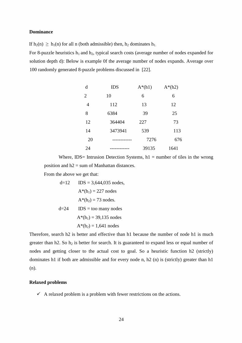
Dominance
If h2(n) ≥ h1(n) for all n (both admissible) then, h2 dominates h1.
For 8-puzzle heuristics h1 and h2, typical search costs (average number of nodes expanded for
solution depth d): Below is example 0f the average number of nodes expands. Average over
100 randomly generated 8-puzzle problems discussed in [22].
d IDS A*(h1) A*(h2)
2 10 6 6
4 112 13 12
8 6384 39 25
12 364404 227 73
14 3473941 539 113
20 ------------ 7276 676
24 ------------ 39135 1641
Where, IDS= Intrusion Detection Systems, h1 = number of tiles in the wrong
position and h2 = sum of Manhattan distances.
From the above we get that:
d=12 IDS = 3,644,035 nodes,
A*(h1) = 227 nodes
A*(h2) = 73 nodes.
d=24 IDS = too many nodes
A*(h1) = 39,135 nodes
A*(h2) = 1,641 nodes
Therefore, search h2 is better and effective than h1 because the number of node h1 is much
greater than h2. So h2 is better for search. It is guaranteed to expand less or equal number of
nodes and getting closer to the actual cost to goal. So a heuristic function h2 (strictly)
dominates h1 if both are admissible and for every node n, h2 (n) is (strictly) greater than h1
(n).
Relaxed problems
A relaxed problem is a problem with fewer restrictions on the actions.
Page 36
25
The cost of an optimal solution to a relaxed problem is an admissible heuristic for the
original problem.
If the rules of the 8-puzzle are relaxed so that a tile can move anywhere, then h1(n)
gives the shortest solution
If the rules are relaxed so that a tile can move to any adjacent square, then h2(n) gives
the shortest solution
Properties of A*
Complete? Yes (unless there are infinitely many nodes with f ≤ f(G) , i.e. step-cost >
ε)
Time/Space? It is the exponential of :bd
Except if: |h (n ) −h *(n ) |≤O (logh *(n ))
Optimal? Yes
Optimally Efficient: Yes (no algorithm with the same heuristic is guaranteed to
expand fewer nodes)
Memory Bounded Heuristic Search: Recursive BFS (RBFS)
How can we solve the memory problem for A*search algorithm?
Idea: Try something like depth first search, but let‟s not forget everything about the
branches we have partially explored.
We remember the best f-value we have found so far in the branch we are deleting.
RBFS changes its mind very often in practice [24], [25].
This is because the f=g+h become more accurate (less optimistic) as we approach the goal.
Hence, higher level nodes have smaller f-values and will be explored first.
Problem: We should keep in memory whatever we can.
2.2.5 Pseudo code for A*
The goal node is denoted by node_goal and the source node is denoted by node_start
It maintains two lists: OPEN and CLOSE:
OPEN consists on nodes that have been visited but not expanded (meaning that successors
have not been explored yet). This is the list of pending tasks:
COLSE consists on nodes that have been visited and expanded (successors have been
explored already and included in the open list, if this was the case).
Put node_start in the OPEN list with f(node_start)=h(node_start) (initialization)
Page 37
26
While the OPEN list is not empty {
Take from the open list the node node_current with the lowest
f(node_current) = g(node_current) + h(node_current)
if node_current is node_goal we have found the solution; break
Generate each state node_successor that come after node_current
for each node_successor of node_current{
Set successor_current_cost= g(node_current) + w(node_current, node_successor)
if node_successor is in the OPEN list {
if g(node_successor) < successor_current_cost continue
} else if node_successor is in the CLOSED list {
if g(node_successor) <successor_current_cost continue
Move node_succssor from the CLOSED list to the OPEN list
} else {
Add node_successor to the OPEN list
Set h(node_successor) =to the heuristic to node_goal
}
Set g(node_successor)= successor_current_cost
Set the part of node_successor to node_current
}
Add node_current to the CLOSED list
}
if(node_current !=node_goal) exit with error ()the OPEN list empty
Comparisons to Dijkstra‟s Algorithm Observation: A* is very similar to Dijkstra‟s algorithm:
Put node_start in the OPEN list with f(node_start)=h(node_start) (initialization)
While the OPEN list is not empty {
Take from the open list the node node_current with the lowest
f(node_current) = g(node_current) + h(node_current)
if node_current is node_goal we have found the solution; break
Generate each state node_successor that come after node_current
for each node_successor of node_current{
Set successor_current_cost= g(node_current) + w(node_current, node_successor)
Page 38
27
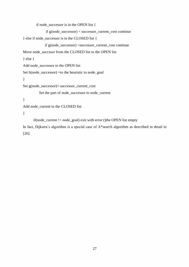
if node_successor is in the OPEN list {
if g(node_successor) < successor_current_cost continue
} else if node_successor is in the CLOSED list {
if g(node_successor) <successor_current_cost continue
Move node_succssor from the CLOSED list to the OPEN list
} else {
Add node_successor to the OPEN list
Set h(node_successor) =to the heuristic to node_goal
}
Set g(node_successor)= successor_current_cost
Set the part of node_successor to node_current
}
Add node_current to the CLOSED list
}
if(node_current != node_goal) exit with error ()the OPEN list empty
In fact, Dijkstra‟s algorithm is a special case of A*search algorithm as described in detail in
[26].
Page 39
28
CHAPTER THREE
RELATED WORKS
In this section, it is tried to review different related works that are vital for my thesis work.
By applying artificial intelligent node to improve the routing protocol performance in router
and core switch is a very new yet an active area, intensive research was recently devoted to
clarify remaining ambiguities, to identify limitations and difficulties, to propose solutions and
to improve the performance of these networks. So some of the work done related to in
artificial intelligence and routing protocol
3.1 Related to Artificial Intelligent
In [27] the authors presented the concepts of knowledge-Define Networking paradigm and
how it operates with combines with Software- Defined Networking, Network Analytics. They
show the basic steps of the main KDN control and described these steps in detail [27]. The
author‟s presents the set of specific relevant uses-cases that illustrate the potential application
of the KDN paradigm and the benefits a Knowledge Plane based on Machine learning may
bring to common networking problems. For two representative use-cases, routing in an
overlay network and resources management in Network Function Virtualization scenario,
they provide experimental results that show the technical feasibility of proposed paradigm.
The authors also discussed[27] the most relevant ones of the challenges such as New
Machine Learning mechanisms, Non-Determistic networks and Standardized datasets.
Finally, the authors‟ conclude on the paper by analyzing the open research challenges
associated with the KDN.
Another remarkable effort was presented in wireless networks throughput enhancement using
AI [28] to quantify the impact of different protocols on AI. The main objective on this paper
is to utilize the correct technique of artificial intelligence in multi-channel network. This
multi-channel reduces interference and improves performance of the network. For achieving
such a goal in wireless environment, the authors used efficient protocol and algorithm called
candidate algorithm. The methodology that describe [28] on this work is three stages. The
first step is to create a model for specific wireless environment, the second step is to choose
the right tool to optimize the performance and the third step is the careful selection of
Page 40
29
performance indicators for routing improvements. After choosing the methodology the
authors conducted experiments in the Linux router real network as well as in the MATLAB.
As a result, the algorithm is able to take routing decisions in a decentralized and
asynchronous fashion. From the experiments, they got the result
According to [29], introduce why intelligence is demanded for evolving the emerging
heterogeneous networks. It described in detail in the introduction fast development of current
internet and Mobile Communication Industry, the system of mobile network operation,
heterogeneous network, worldwide Interoperability for Microwave Access and enhanced
Node base station [29]. On this paper [29], it also describes issues of heterogeneous network
that can be benefit from AI based techniques like self-configuration, self-healing and self-
optimization. They survey and discussed the AI-related self-organizing networks techniques
in heterogeneous networks by classifying them base on the type of AI techniques. Techniques
used on this paper machine learning, genetic algorithm, swarm intelligence and ant colony,
fuzzy system, artificial neural networks and Markov models and Bayesian-based games [29].
New challenges and opportunities also described in detail in this paper.
Additionally, in [30] described solving routing problem in order to maintain continuous
network transmission without any loss of packets. On this paper it is described about
networking routing and router and other related work done in Artificial Intelligence which
tackles routing problem such as shortest path algorithm, generic algorithm, distributed AI and
agent based routing and algorithmic resource allocation methods. The author also presented
the architecture and design of the proposed system and evaluated the performance of
algorithm test. Finally, the authors concluded and suggested on the paper for future work.
Network routing problems also described [31] by survey on artificial intelligent. In this paper,
it focus giving generic problem description and the situations of today‟s network, different
types of routing protocol and techniques, artificial intelligent which tackles different types of
routing problems in details.
In [32], discuss possible improvement in wireless sensor network routing and security
through the employment of concepts coming from artificial intelligent area. The paper
highlights routing in wireless sensor network, security in wireless sensor networks, related
works, and defense mechanism for security in wireless sensor network using game theory.
In [33], attempts to encourage the use of artificial intelligence techniques in wireless sensor
nodes. This paper is organized with introduction, designing the network topology,
introducing neurons in sensor nodes, perform evaluation by simulation.
Page 41
30
3.2 Related to Routing protocols
This part presents paper worked on related to routing protocol networking. In this [34]
discussed the properties and review the main instance of network routing algorithms whose
bottom-up design. Briefly introduces network routing and discussed the general
characteristics of routing and the associated challenges for each of one of the considered
network classes. The paper [34] also provides a comprehensive set of classification features
that they would use to characterize routing protocols. The paper also described the ant and
bee colony behaviors that have fueled the design of so many networks routing algorithm.
They discuss in some detail [34] two main implementation, Bee Hive for wired connection
networks and Bee Adhoc for MANETs.
In [35], proposed an open architecture to enable the pc-based router to support multiple tasks
beyond solely routing and forwarding.
3.3 Research Gaps
Based on the finding of related works covered above, following are the areas identified that
require significant research to be done:
Performance: This is an open challenge to optimize and improve the performance of routing
protocol.
Routing: The routing protocols should be able to update routing tables dynamically according
to topology changes. Routing protocols of previous common Adhoc networks were partly fail
to provide a reliable communication. Therefore, there is a need of developing new routing
algorithms and networking model for constructing a flexible and responsive integration
model. One of the biggest challenges for researchers is to find out the best routing protocols
from the existing one and selecting search algorithms from AI to suggest an efficient routing
algorithm that can work by combining artificial intelligent with routing protocol.
Path Planning: Thus, new algorithms/methods in dynamic path planning are required to
improve routing protocol.
Based on the above research gabs, trying find from search algorithm which is best and from
routing protocol in the existing one.
Page 42
31
CHAPTER FOUR
ENHANCED INTERIOR GATEWAY ROUTING PROTOCOL
4.1 Introduction
Enhanced Interior Gateway Routing Protocol (EIGRP) is a vendor specific protocol. It is
CISCO‟s proprietary protocol that is an improved version of the interior gateway routing
protocol (IGRP). EIGRP is being used as a more scalable protocol in both medium and large
scale networks since 1992. EIGRP is said to be an extensively used IGRP where route
computation is done through Diffusion Update Algorithm (DUAL). EIGRP can also be
considered as hybrid protocol because of having link state protocol properties. Even if EIGRP
is CISCO‟s proprietary protocol, there are some advantages than other routing protocol
provides by EIGRP [2], [6] such as: easy to configure, loop free routes are offered, it keeps a
backup path in the network to get the destination, and multiple network layer protocols are
included, EIGRP convergence time is low and it is responsible for the reduction of the
bandwidth utilization, it can work with Variable Length Subnet Mask (VLSM) and Class Less
Inter Domain Routing (CIDR) and EIGRP also supports the routing update authentication.
Because of the EIGRP is preferable from other routing protocols to improve the routing
performance of routers and core switches by combining A* search algorithm. The
disadvantage of this protocol is considered as Cisco proprietary routing protocol and routers
from other vendors are not able to utilize EIGRP.
4.2 Protocol Structure
3Table 4.1: Protocol structure of EIGRP
Bits 0 8 16 31
Version Opcode Checksum
Flags
Sequence Number
Acknowledge Number
Autonomous System Number
Type Length
Page 43
32
Table 4.1 demonstrates the protocol structure of EIGRP and each field is described below[13]
and [36]:
Version: Indicates the version of EIGRP
Opcode: The Operation code usually specifies the message types. For
example: 1. Update, 2. Reserved, 3. Query, 4. Reply, 5. HELLO, 6. IPX-SAP.
Checksum: Identifies IP checksum that is calculated by using the same
checksum algorithm.
Flag: First bit (0x00000001) is used to form a new neighbor relationship and is
known as initialization bit. Second bit (0x00000002) is used in proprietary
multicast algorithm and is termed as conditional receive bit. There is no
function for the remaining bits.
Sequence and Acknowledge Number: Passing messages securely and
reliably.
Autonomous System: It explains the independent system numbers which is
found in EIGRP domain. The separate routing tables are found to be associated
with each AS because a gateway can be used in more than one AS. This field is
used for specifying the exact routing table.
Type: Determine the type field values which are:
- 0x0001-EIGRP Parameters (Hello/Hold time)
- 0x0002-Reserved
- 0x0003-Sequence
- 0x0004-Software Version of EIGRP
- 0x0005-Next Multicast Sequence
- 0x0012-IP Internal Routes
- 0x0013-IP External Routes
Length: Describes the length of the frame.
Page 44
33
4.3 Technique of EIGRP
EIGRP has the following four procedures. These are:
i. Neighbor Discovery/Recovery
ii. Reliable Transport Protocol (RTP)
iii. Diffusion Update Algorithm (DUAL)
iv. Protocol Dependent Modules (PDM)
4.3.1 Neighbor Discovery/Recovery
The neighbor discovery/recovery technique lets the routers and core-switches to gain
knowledge about other routers and core-switches which are directly linked to their networks
using the routing information from the routing table [37], [38]. If the neighbors become
unreachable and inaccessible, it is very important for them to be able to discover it. This is
done by sending HELLO packets at intervals with a comparatively low overhead. After
receiving a HELLO packet from its neighbors, the router and core-switches ensures that its
neighboring routers and core-switches are aware of the state and the exchange of routing
information is possible. In case of high speed networks, the default value for HELLO time is 5
seconds. Every HELLO packet advertises the holding time for maintaining the relationship.
The particular time when the neighbor judges the sender as alive is called Hold time. 15
seconds is the default value of hold time. If the EIGRP router and core-switches does not
accept any HELLO packets from the adjacent router and core-switches during the hold time
interval, the adjacent router or core-switch is removed from the routing table. Thus, hold time
is not only to be used for detecting the loss of neighbors but also for discovering neighbors.
On multipoint interfaces, HELLO/Hold time for networks with link speed T-1 is usually set to
60/180 seconds [39]. The convergence time lengthened with the extension of the HELLO
interval time. Nevertheless, HELLO intervals with long duration are possible to be
implemented in congested networks of several EIGRP routers. In a network, the HELLO/Hold
time differs among the routers. A rule of thumb states that the hold time should be equal to
thrice of the HELLO time [40]. Table 4.2 presents the default values of HELLO and hold
times for EIGRP [40].
Page 45
34
4Table 4.2: EIGRP interval time for Hello and Hold
Bandwidth Example
Link
Hello Interval
Default Value
Hold Interval Default value
1.544
Mbps or
Slower
Multipoint
Frame
Relay
60 seconds 180 seconds
1.544
Mbps
T1,
Ethernet
5 seconds 15 seconds
4.3.2 Reliable Transport Protocol
The routing updates information is used to make the sorting in series using the sequence
number. RTP allows intermixed transmission of multicast or unicast packets [8], [10]. The
certain EIGRP packets need to be transmitted reliably while others do not require [41]. Hence
reliability can be ensured according to the requirement. For instance, in case of Ethernet,
which is a multi-access network and provide multicasting capacity, it is not vital to transmit
HELLOs reliably to other neighbors.
Therefore, by sending a single multicast HELLO, EIGRP informs receivers, that the packets
are not needed to be acknowledged. But updating packets need to be acknowledged when they
are sent. RTP has a condition to transmit the multicast packet very fast when there are some
unacknowledged packets left.
For this reason, in the presence of varying speed links, this helps to ensure that the
convergence time are low.
4.3.3 Diffusion Update Algorithm
The Diffusion Update Algorithm (DUAL) uses some requirements and concepts which has a
significant role in loop-avoidance mechanism as follows:
Feasible Distance (FD)
The lowest cost needed to reach the destination is usually termed as the feasible
distance for that specific destination.
Page 46
35
Reported Distance (RD)
A Router has a cost for reaching the destination and it is denoted as reported distance.
Successor
A Successor is basically an adjacent router which determines the least-cost route to the
destination network.
Feasible Successor (FS)
FS is an adjacent router which is used to offer a loop free backup path to the
destination by fulfilling the conditions of FC.
Feasible Condition (FC)
After the condition of FD is met, FC is used in order to select the reasonable
successor. The RD advertised by a router should be less than the FD to the same
destination for fulfilling the condition.
Mainly the DUAL is responsible for doing all route calculations in EIGRP. The main task of
DUAL includes keeping a table, known as topology table, which includes all the entries found
from the loop-free paths advertised by all routers and core-switches. DUAL selects the best
loop-free path (known as successor path) and second best loop free path (known as feasible
path) from the topology table by using the distance information and then save this into the
routing table. Successor is the neighbor of the least cost route to the destination.
By using the topology table, DUAL can check if another best loop-free path is available.
DUAL does this when the successor path is inaccessible. This path is recognized as feasible
path. The reasonable path is selected if it satisfies the FC. The FC condition is possible to be
satisfied if the neighbor's RD to a network is less than the RD of the local router. When a
neighbor router meets the FC condition, it is then termed as FS.
In case of having no loop-free path in the topology table, re-calculation of the route must take
place and then the DUAL inquire its neighbors. This occurs during re-calculation for
searching a new successor. Although, the re-calculation of the route does not seem to be
processor-intensive, it may have an effect on the convergence time and consequently, it is
useful for avoiding needless computations. In case of having any FS, DUAL is used for
avoiding any needless re-computation. If we consider Fig 4.1, we will be able to understand
how the DUAL converges. This example aims at router K for the destination only. The cost of
K (hops) coming from each router is presented below [38]:
Page 47
36
3Fig. 4.1: DUAL placed in the network [38].
In Fig. 4.2, the link from A to D fails. When the loss of the FS occurs, a message goes to the
adjacent router sent by D. This is received by C. Then C determines if there is any FS. In case
of having no FS, C needs to begin a new route calculation by entering the active state. The
cost from router C to router K is 3 and the cost from router B to router K is 2. Hence it is
possible for C to switch to B. There is no effect on router A and B for this change. Thus they
have no contribution in finding the reasonable successor.
Page 48
37
4Fig. 4.2: Failure Link of Network Topology [38].
5Fig. 4.3: Failure Link of Network Topology [38].
Now, observe the case in fig. 4.3, where the link from A to B fails. B is found in this scenario
to have been lost its successor and thus no FS exists. Router C cannot be treated as FS to B, as
the cost of C is more than the present cost of B. Consequently, the route computation is to be
performed by B and for this, B sends a query to its neighbor C. In reply, C acknowledges the
query because C does not need to perform the route calculation.
When B receives the reply, it assumes that all the adjacent routers have processed the link
failure. B can choose C for getting the destinations as its successor with a cost of 4. It didn‟t
have any effect on A and D for changing the topology and thus, C needed just to reply on B.
4.4 EIGRP Metrics
By using total delay and the minimum link bandwidth, it is possible to define the routing
metrics in EIGRP. The metrics, which consists of bandwidth, reliability, delay, and load are
considered to be used for the purpose of calculating the preferred path to the networks. The
EIGRP routing update takes the hop count into account though EIGRP does not include hop
count as a component of composite metrics. The total delay and the minimum bandwidth
metrics can be achieved from values [39] which are put together on interfaces and the formula
used to compute the metric is followed by:
Page 49
38
∗ [( ∗ ∗
∗ )] ∗
( )
For weights, the default values are:
=1, =0, =1, =0, =0,
Put those values in equation 1.
∗ ( ) ( )
If =0, the formula trims down like
256*[(K1*Bw+ ∗
∗ )
EIGRP uses to calculate scale bandwidth is:
(
( )) ∗ ( )
Where, ( ) is in kilobits and represents the minimum bandwidth on the interface to
destination.
Bw= Bandwidth
The formula that EIGRP uses to calculate scale delay is:
( ) ∗ ( )
Where D (n) represents in microseconds and sum of the delays configured on
the interface to the destination.
4.5 EIGRP Convergence
In fig. 4.4, that the link from R3 and R5 goes down and at the same time R3 identifies the
failure of the link. There is no FS present in the topology database and hence the role of R3 is
to be entered into the active convergence. R4 and R2, on the other hand, are the only
neighbors to R3. Given that, there is no availability of route with lower FD, R3 sends a
message to both R4 and R2 for gaining a logical successor. R2, for acknowledgement, replies
to R3 and indicates that there is no availability of successor.
On the other hand, R3 gets positive acknowledgement from R4 and the FS with higher FD
becomes available to R3. The distance and new path is allowed by R3 and then added to the
Page 50
39
routing table. Followed by R2 and R4 are sent an update about the higher metric. In the
network, all the routes converge when the updates are reached to them.
6
Fig. 4.4: Network topology of EIGRP
Page 51
40
CHATER FIVE
RESULTS AND DISCUSSIONS
5.1 Introduction
Several software packages exist for running computer-based simulation modeling (e.g. multi-
method modeling, NS-2 simulator, OPNET and other) that makes all the modeling almost
effortless.
In this thesis, Network Simulator 2 (NS-2) is used. NS-2 is Discrete-event driven network
simulation, Object Oriented which is an extended Tcl (OTcl) interpreter that can be written in
C++ and OTcl where C++ implements the code that executed frequently and OTcl configures
the system. This simulator (NS-2) can be run on UNIX or Linux and Windows platforms
under some configurations and settings.
NS-2 can be used for parallel and distributed simulation: PDNS. NS-2 provides emulation
functionalities. NS-2 comes closer to reality than other simulators [42]. A good simulation
design, good results can be achieved with NS-2 [42]. Even if, the OPNET is not used in this
simulation it is also a simulator built on top of discrete event system (DES) and it simulates
the system behavior by modeling each event in the system and processes it through user
defined processes. OPNET is very powerful software to simulate heterogeneous network with
various protocols.
5.2 Structure of NS-2
This network simulator is characterized by these parameters [43], [44].
Free
Almost all network components are implemented
Active contributions from researchers
Easy to modify and/or add new functions
NS-2 network simulator is composed of the following main components. These are
1. Application
Those applications in NS-2 are communication instigator where they poke the agent to which
they‟re attached
Introduction of Process class
Page 52
41
Models any entity that is capable of receiving, requesting or processing data
Two basic types:
class Process : public TclObject[ns-2.29/common/ns-process.h]
1. class Application: public Process [ns-2.29/apps/app.h]
2. class Traffic Generator: public Application [ns-2.29/tools/trafgen.h]
This application assumes attached to a TCP Agent
start(), stop(), send(), recv()
E.g. class TelnetApp
[ns-2.20/apps/telnet.h]
Schedule agent_->sendmsg()calls based on exponential inter-arrival timer
Traffic Generator
Assumes attached to a UDP Agent
init(), next_interval()
E.g. class POO_Traffic
[ns-2.29/tools/pareto.cc]
Schedule bursts of packets (Pareto on-off source)
2. Agent
Packet generator/consumer
TCP/UDP stacks
timeout(),send(), etc
Allocate and schedule packets
recv(), etc
Callback to app_to notify of data
Subtype of Connector
class Agent: public Connector
[ns-2.29/common/agent.h, …/tcl/lib/ns-agent.tcl]
class Tcp Agent: public Agent
class Full Tcp Agent: public Tcp Agent
class Udp Agent: public Agent
3. Node
Addressable entity built from classifiers
Distributes incoming data to agents
Page 53
42
Distributes outgoing data to links
Simplest unicast case has address and port classifiers, others may have more
Node, LanNode, etc derived from ParentNode
7Fig. 5.1: Nodes and agents integration
4. Link
Are set of queues in the NS-2 simulation program or code.
An OTcl amalgam of C++ objects[ns-2.29/tcl/lib/ns-link.tcl]
class Simple Link–superclass Link
Simulator instproc duplex-link{ n1 n2 bw delay type args }
More complex links may have complex link delay/bw characteristics…[ns-
2.29/link/delay.h]
class Link Delay: public Connector
Multiple queue_ elements [ns-2.29/queue/{queue.h,red.h,…}]
class Queue: public Connector
class RedQueue : public Queue
Page 54
43
8Fig. 5.2: Link example and some functions in it
Basically, NS-2 is composed of
1. NS2: the simulator itself
2. NAM: Network animator. Visualized trace tool (not really).
Nam editor: GUI interface to generate ns scripts
3. Pre-processing:
Traffic and topology generators
4. Post-processing:
Simple trace analysis, often in Awk, Perl (mostly), or Tcl
9
10Fig. 5.3: Architecture of NS-2
Page 55
44
5.3 Design and Analysis in NS-2
NS-2 uses the programs or codes written in C++ or TCL to simulate the designed network.
11Fig. 5.4: Designing Steps
5.4 Simulation Study
The protocols used here is EIGRP routing protocol and A * search algorithm. The routing
protocol and the search algorithm together are evaluated based on the quantitative metrics
such as convergence duration, packet delay variation, end to end delay, jitter and throughput.
5.5 Network Topology
According to [45] Network topology is the arrangement of various elements of a computer
network. It is typically described as either physical or logical. Different placements of network
components such as device location and the shape of cabling layout are part of physical topology.
A physical network topology refers to the actual layout of nodes and other networking
devices. On the other hand, Logical topology illustrates how the data passes through the network
regardless of the physical design or refers to the communication methods used by different
components. In many cases, network topologies may be identical, but the distances between
nodes, physical interconnections, transmission rates and signal types will still be different. For
this simulation purpose, mesh topology, all node in the network are connected to every other
node, is used. Because mesh topology have the following advantages that describes in [45]:
A mesh network is highly reliable because of redundant multiple paths between nodes.
A failure of a single node not affect network operations.
Nodes can be added or removed without affecting the network.
Create
Network Model
By writing TCL code
Choose Parameters and
measurement units
Run
Simulation
Analysis
Result
Page 56
45
For this simulation study mesh network topology was selected, and then designed wired
network topology consisting of 12 nodes. Choosing of these 12 number of node is to show
easily and better understanding path from source to destination on the physical network
topology, to minimize the execution time of simulation [42] (when the number of node
increase, simulation execution time is increased, the time taken to exchange data between
node is not only determined by the size of the simulation and number of nodes used, but also
by the speed at which the network hardware can exchange data) and to exchange packets
between the nodes as they come within hearing range of one another.
A wired network topology consisting of 12 nodes has been designed as shown in Fig. 5.5
below.
12Fig. 5.5: Wired network topology with 12 nodes
When the communication between those nodes starts the path that a packet follows is
determined by the algorithm used to design this topology. To demonstrate this Fig 5.6 is more
suitable.
Page 57
46
13
Fig. 5.6: Wired network topology with source and destination scenario
In this topology there are two different communications as indicated by the green (upper) and
red (lower) colors. Thus, the red color which starts from node 0 as a source and transmitted it
to the destination as node 5 with minimum path of four. The other one is the green color that
starts from node 1 as a source and destination to node 5.
Both of those communications are UDP with CBR application traffic. As shown in the
topology there is no failure and the next Fig.5.7 shows what happened when one
communication link fails and how the algorithm reroutes to find out the next shortest path to
overcome the failure.
14Fig. 5.7: Wired network topology communication line failure
Page 58
47
In Fig 5.7, the line between the nodes 11 and 5 failed. Due to this failure the route between
the nodes 0 to 5 and 1 to 5 automatically changed by the algorithm used to create another best
and shortest path. Even if, there are additional paths but the algorithm selects the shortest
path for the two communications.
In such cases EIGRP with A* search algorithm used to find out the paths and redirect the
communication to the best and shortest path. In this topology EIGRP with A * search
algorithm used and as showed above in the figure when the link failure happens the packets
forwarded to their destination from where they were before the failure happens. So, no need
of sending them again from their source.
5.6 Measurements
In this section, the main measurement units of the performance metrics, such as Packet-loss,
delay and throughput are done from the acquired results of Discrete Event Simulation which
is network simulation 2 (NS2).
5.7 Simulation Results and Analysis
In this section, the simulation results with a brief description and explanation is presented.
There are two network models, which are configured and run using network simulator 2
(NS2). The first one is EIGRP with its original search algorithm which is Dijkstra, the second
one with EIGRP with A * search algorithm using the concept of artificial node creation that
can learn from the network.
In the following table the results are presented.
5Table 5.1: Simulation results
EIGRP Protocol and EIGRP with A*Search Algorithm
Parameter/Metrics EIGRP EIGRP with A * search
algorithm
Throughput(Kbps) 200,465.48 216,481.26
Packet-loss 8 6
Delay 0.23448 0.23338
Page 59
48
Using the three main parameters to measure performance of routers and core-switches the
simulation result is done. The above tabular data is organized and gathered from the topology
with 12 nodes and using CBR and UDP application and traffic. Throughput, Packet-loss and
Delay are the main parameters chosen for the simulation.
The main reason for performance enhancement came from the above result is because of
EIGRP uses minimal consumption of bandwidth when the network is stable, efficient use of
bandwidth during convergence, rapid convergence, support for Variable Length Subnet Mask
(VLSM) and Classless Iner- Domain Routing(CIDR) and complete independence from routed
protocols. And also A* search algorithm choose the best path by avoid expanding path, it
scan the area only in the direction of destination and same time.
So when combine this EIGRP and A* search algorithm, it can be get better performance and
improved result based on the above metrics (parameters). The cost also minimize when using
EIGRP and A* search algorithm. This is because EIGRP uses the metric the combinations of
bandwidth and delay and A* search algorithm use best path to reach the destination from the
source, this minimize time to search. Generally, the performance improvement induced by
the controller depends on the topology and the available resources, such as the number of
nodes and the channel bandwidth.
These parameters are mainly analyzed in detail. So, starting from the table above each of the
described as follows.
Page 60
49
15Fig. 5.8: Throughput over EIGRP and EIGRP with A* search algorithm
The throughput is a key parameter to determine the rate at which total data packets are
successfully delivered through the channel in the network.
From the above Fig. EIGRP with A * search algorithm has a promising improvement of
throughput over the network topology given for simulation. So, using the A * search
algorithm is best effective and has a measurable difference than using EIGRP. Introducing an
artificial node using the A * search algorithm improves the throughput of the network.
A typical method of performing a measurement is to transfer a 'large' file from one system to
another system and measure the time required to complete the transfer or copy of the file. The
throughput is then calculated by dividing the file size by the time to get the throughput in
megabits, kilobits, or bits per second.
Unfortunately, the results of such an exercise will often result in the good put which is less
than the maximum theoretical data throughput, leading to people believing that their
communications link is not operating correctly. In fact, there are many overheads accounted
for in addition to transmission overheads, including latency, TCP Receive Window size and
other system limitations. That means the calculated good put does not reflect the maximum
achievable throughput.
Page 61
50
16Fig. 5.9: Packet loss over EIGRP and EIGRP with A* search algorithm
From the above Fig. it is clear that EIGRP with A * search algorithm has a better performance
on packet loss due to many reasons. So, using the network topology with 12 nodes and a
routing algorithm of EIGRP with optimal path finding of A * is better than EIGRP.
Packet loss occurs when one or more packets of data travelling across a computer network fail
to reach their destination. Packet loss is typically caused by network congestion. Packet loss is
measured as a percentage of packets lost with respect to packets sent.
Page 62
51
17Fig. 5.10: Delay over EIGRP and EIGRP with A* search algorithm
Delay variation is measured by the difference in the delay of the packets. This metric has huge
influence on the manners of video applications. Delay for any kind of network or
communication is a headache. From Fig.5.10, it is clear that the routing protocol EIGRP with
A * search algorithm minimizes the delay and improves performance over EIGRP. By using a
routing protocol that supports A * search algorithm it is possible that a Delay Tolerant
Network (DTN) can be created.
0.2328
0.233
0.2332
0.2334
0.2336
0.2338
0.234
0.2342
0.2344
0.2346
Delay
Delay
EIGRP
EIGRP with A * star searchalgorithm
Del
ay
(S
eco
nd
)
Page 63
52
CHAPTER SIX
CONCLUSIONS AND FUTURE WORKS
In this thesis, introducing an artificial node to the routing protocol which is EIGRP is done
using A * search algorithm. The artificial intelligence search algorithm A * defined and
described with the comparison of the other search algorithms and path findings so that, it helps
to introduce the artificial intelligence node. It is also presented analysis of routing protocols
such as EIGRP, OSPF. The study has been done in the same network with different protocols.
Performance has been measured on the basis of some parameters that aimed to figure out the
effects of routing protocols and the search algorithm selected to it.
Implementation of EIGRP with A * search algorithm shows that it is better and effective than
using the normal EIGRP routing protocol. This is because, EIGRP with A * finds the best and
shortest path, minimizes network overload by learning the network fast and lookup quickly.
The simulation results have shown that the throughput in the combination of EIGRP with A *
search algorithm is much higher than that of EIGRP routing protocol. This result also depicted
that throughput can be updated and improved by using EIGRP with A * search algorithm. The
simulation result also shown that delay of EIGRP network is relatively greater that of EIGRP
with A * search algorithm. As a result, data packets in EIGRP with A * search algorithm
network reach faster to the destination. In the context of packet loss, EIGRP with A * search
algorithm is slightly lower than that of EIGRP routing protocol.
So, the combination of EIGRP with A * search algorithm used to create and introduce the
artificial intelligent node and EIGRP by itself has been analyzed and studied in detail. By
combining EIGRP and A * search algorithm, I have come across that the combined
implementation of EIGRP and A * search algorithm performs better than EIGRP routing
protocol.
In future, a research work can be done on the security analysis of EIGRP. Because of the
security vulnerability of the protocol in it is hybrid and mainly dependent on the venders
device and the integration of EIGRP with the defined A * search algorithm in device level.
Page 64
53
References
[1] “Basic Routing concepts and protocols Explained.”
http://www.computernetworkingnotes.com/ccna-study-guide/basic-routing-concepts-
and-protocols-explained.html.
[2] S. G. Thorenoor, “Dynamic routing protocol implementation decision between EIGRP,
OSPF and RIP based on technical background using OPNET modeler,” 2nd Int. Conf.
Comput. Netw. Technol. ICCNT 2010, pp. 191–195, 2010.
[3] “Performance Analysis of EIGRP and OSPF for Different Applications using
OPNET.” .
[4] A. Bright, M. Adamu, A. Franklin, and M. Asante, “Performance Analysis of
Enhanced Interior Gateway Routing Protocol (EIGRP) Over Open Shortest Path First
(OSPF) Protocol with Opnet,” Int. J. Adv. Comput. Sci. Appl., vol. 7, no. 5, pp. 111–
117, 2016.
[5] K. Terms, Introduction to Dynamic Routing Protocols Objectives. .
[6] “RFC 7868 - Cisco‟s Enhanced Interior Gateway Routing Protocol (EIGRP).” .
[7] “https://www.ietf.org/rfc/rfc2328.txt.” .
[8] “https://tools.ietf.org/html/rfc1058.” .
[9] “https://tools.ietf.org/html/rfc7868.” .
[10] “https://tools.ietf.org/html/rfc2453.” .
[11] P. Kannagi, “(ospf & eigrp),” vol. 1, no. 3, pp. 13–22, 2013.
[12] M. Hutter, “Artificial Intelligence: Overview,” (Canberra ACT 0200 Australia). pp. 1–
15.
[13] V. Sharma, R. Narula, and S. Khullar, “Performance Analysis of IEEE 802 . 3 using
IGRP and EIGRP Routing Protocols,” Int. J. Comput. Appl. (0975 – 8887), vol. 44, no.
April, pp. 21–25, 2012.
[14] G. Jain, T. Hadpawat, and D. Vaya, “Performance Evaluation of Authenticate (MD5,
SHA) Routing Traffic over EIGRP and OSPF with IPV6,” Int. J. Comput. Appl., vol.
176, no. 8, pp. 26–29, 2017.
[15] D. Comer, “Internetworking With TCP / IP,” Internetworking Research And
Experience. 2005.
[16] N. Pandey, “Simulation Based Comparative Study on EIGRP / IS-IS and OSPF / IS-
IS,” vol. 3, no. 2, pp. 204–214, 2015.
Page 65
54
[17] K. Raghu, “Performance Analysis of Optimal Path using DSR and NFPQR Protocols,”
vol. 4, no. 5, pp. 68–73, 2017.
[18] W. Mai et al., “Proceedings of the International Conference on Engineering , Science ,
and Industrial Applications.”
[19] S. Chen, “The A * Search Algorithm'' http://db.cs.duke.edu//courses/fall
11/cps149s/notes/a_star.pdf.
[20] M. Sniedovich, “Control and Cybernetics,” Control Cybern., vol. 35, no. 3, pp. 87–92,
2006.
[21] K. R. Chowdhary, “Artificial Intelligence ( Heuristic Search)''
http://www.dsi.unive.it/atorsell/AI/03-heuristicssearch.pdf
[22] D. Partridge, RussellNorvig_Solutions. “Artificial Intelligence: A Modern Approach,
Third edition” 2002.
[23] G. Gigerenzer and W. Gaissmaier, “Heuristic Decision Making,” Ssrn, 2010.
[24] “Artificial Intelligence_ Memory bounded heuristic search.” .
[25] “Artificial Intelligence - Neeta Deshpande, Nanda Yadav - Google Books.” .
[26] “LLE Algorithm Pseudocode,” pp. 1–2.
[27] A. Mestres et al., “Knowledge-Defined Networking,” pp. 1–8, 2016.
[28] S. Ahmad, R. M. Nadeem, B. Ehsan, M. Ullah, and A. B. Siddique, “Wireless
Networks Throughput Enhancement Using Artificial Intelligence,” Indian J. Sci.
Technol., vol. 10, no. 26, pp. 1–5, 2017.
[29] X. Wang, X. Li, and V. C. M. Leung, “Artificial intelligence-based techniques for
emerging heterogeneous network: State of the arts, opportunities, and challenges,”
IEEE Access, vol. 3, pp. 1379–1391, 2015.
[30] A. Oloduowo, A. Babalola, and A. Daniel, “Solving Network Routing Problem Using
Artificial Intelligent Techniques,” Br. J. Math. Comput. Sci., vol. 17, no. 3, pp. 1–9,
2016.
[31] H. Bai, “A Survey on Artificial Intelligence for Network Routing Problems,” pp. 1–10,
2017.
[32] E. Sandeep Kumar, “Improving WSN routing and security with an artificial
intelligence approach,” CEUR Workshop Proc., vol. 1334, pp. 62–71, 2014.
[33] F. J. Molina, A. Barbancho, J. Barbancho, and C. Leo, “Using artificial intelligence in
routing schemes for wireless networks,” Comput. Commun., vol. 30, pp. 2802–2811,
2007.
[34] M. Farooq and G. A. Di Caro, “Routing Protocols for Next-Generation Networks
Page 66
55
Inspired by Collective Behaviors of Insect Societies: An Overview,” Swarm Intell., pp.
101–160, 2008.
[35] V. Tanyingyong, M. Hidell, and P. Sj, “Improving Performance in a Combined Router
/ Server.”
[36] E. S. Lemma, S. A. Hussain, and W. W. Anjelo, “Performance Comparison of EIGRP /
IS-IS and OSPF / IS-IS,” Electr. Eng., no. November, 2009.
[37] I. Basics, B. Basics, R. Basics, N. M. Basics, F. Relay, and D. Technologies,
“Internetworking Technology Handbook,” 2005.
[38] M. N. Islam and A. U. Ashique, “Simulation Based EIGRP over OSPF Performance
Analysis,” Bth.Se, 2010.
[39] “http://www.cisco certification academy.com”/Enhanced-Interior-Gateway-Routing-
Protocol-EIGRP.pdf .
[40] S. K. Sahoo, “ANALYSIS OF ROUTING PROTOCOLS By.”
[41] Rismawati, “International journal of scientific & technology research IJSTR.”
2012.
[42] S. G. Gupta, M. M. Ghonge, P. D. Thakare, and P. M. Jawandhiya, “Open-Source
Network Simulation Tools: An Overview,” Int. J. Adv. Res. Comput. Eng. Technol.,
vol. 2, no. 4, pp. 1629–1635, 2013.
[43] P. Models, “CDA6530: Performance Models of Computers and Networks.”
[44] K. Fall and K. Varadhan, “The network simulator (ns-2),”
Http://Www.Isi.Edu/Nsnam/Ns. 2007.
[45] Pawan K. Bhardwaj, A+, NETWORK+, SECURITY+ EXAMS. 1386.
Page 67
56
Annex A: Sample source code for the topology used. set ns [new Simulator]
set nr [open throold.tr w]
$ns trace-all $nr
setnf [open throold.nam w]
$ns namtrace-all $nf
proc finish { } {
global ns nr nf
$ns flush-trace
close $nf
close $nr
execnamthroold.nam&
exit 0
}
for { set i 0 } { $i < 12} { incr i 1 } {
set n($i) [$ns node]}
for {set i 0} {$i < 8} {incr i} {
$ns duplex-link $n($i) $n([expr $i+1]) 1Mb 10ms DropTail }
$ns duplex-link $n(0) $n(8) 1Mb 10ms DropTail
$ns duplex-link $n(1) $n(10) 1Mb 10ms DropTail
$ns duplex-link $n(0) $n(9) 1Mb 10ms DropTail
$ns duplex-link $n(9) $n(11) 1Mb 10ms DropTail
$ns duplex-link $n(10) $n(11) 1Mb 10ms DropTail
$ns duplex-link $n(11) $n(5) 1Mb 10ms DropTail
$ns duplex-link $n(11) $n(6) 1Mb 10ms DropTail
Page 68
57
set udp0 [new Agent/UDP]
$ns attach-agent $n(0) $udp0
set cbr0 [new Application/Traffic/CBR]
$cbr0 set packetSize_ 500
$cbr0 set interval_ 0.005
$cbr0 attach-agent $udp0
set null0 [new Agent/Null]
$ns attach-agent $n(5) $null0
$ns connect $udp0 $null0
set udp1 [new Agent/UDP]
$ns attach-agent $n(1) $udp1
set cbr1 [new Application/Traffic/CBR]
$cbr1 set packetSize_ 500
$cbr1 set interval_ 0.005
$cbr1 attach-agent $udp1
set null0 [new Agent/Null]
$ns attach-agent $n(5) $null0
$ns connect $udp1 $null0
$ns rtproto DV
$ns rtmodel-at 10.0 down $n(11) $n(5)
$ns rtmodel-at 15.0 down $n(7) $n(6)
$ns rtmodel-at 30.0 up $n(11) $n(5)
$ns rtmodel-at 20.0 up $n(7) $n(6)
$udp0 set fid_ 1
$udp1 set fid_ 2
Page 69
58
$ns color 1 Red
$ns color 2 Green
$ns at 1.0 "$cbr0 start"
$ns at 2.0 "$cbr1 start"
$ns at 45 "finish"
$ns run
Sample AWK source code for throughput calculation
BEGIN {
recvdSize = 0
startTime = 0
stopTime = 500
}
{
event = $1
time = $2
node_id = $3
node_id = $4
pkt_size = $6
level = $5
# Store start time
if ($1 == "r" && $5 == "cbr" &&pkt_size = 500) {
if (time <startTime) {
startTime = time
}
Page 70
59
}
# Update total received packets' size and store packets
arrival time
if ($1 == "r" && $5 == "cbr" &&pkt_size = 500) {
if (time <stopTime) {
stopTime = time
}
# Rip off the header
#hdr_size = pkt_size % 512
#pkt_size -= hdr_size
# Store received packet's size
recvdSize += pkt_size
}
#printf("Value of the number of packets",recvdSize)
}
END {
printf("%10s %10g",event, time)
printf("Value of the number of packets %d",recvdSize)
printf("Average Throughput[kbps] = %.2f\t\t
StartTime=%.2f\tStopTime=%.2f\n",(recvdSize/(stopTime-
startTime))*(8/1000),startTime,stopTime)
}
Delay calculation AWK source code
BEGIN {
highest_packet_id = 0;
Page 71
60
}
{
action = $1;
time = $2;
node_1 = $3;
node_2 = $4;
src = $5;
flow_id = $8;
node_1_address = $9;
node_2_address = $10;
seq_no = $11;
packet_id = $12;
if ( packet_id>highest_packet_id ) highest_packet_id =
packet_id;
if ( start_time[packet_id] == 0 ) start_time[packet_id] =
time;
if ( action != "d" ) {
if ( action == "r" ) {
end_time[packet_id] = time;
}
} else {
end_time[packet_id] = -1;
}
}
Page 72
61
END {
for ( packet_id = 0; packet_id<= highest_packet_id;
packet_id++ ) {
start = start_time[packet_id];
end = end_time[packet_id];
packet_duration = end - start;
if ( start < end ) printf("%f %f\n", start, packet_duration);
}