Faculty of Science and Technology MASTER’S THESIS · Comparisons Study of S-Lay and J-Lay Methods...

Faculty of Science and Technology

MASTER’S THESIS

Study program/ Specialization: Offshore Technology/ Marine and Subsea Technology

Spring semester, 2013

Confidential

Writer :

Jihan Herdiyanti

…………………………………………

(Writer Signature)

Faculty supervisor : Prof. Ove Tobias Gudmestad

External supervisor : Per Richard Nystrøm (IKM Ocean Design)

Title of thesis:

Comparisons Study of S-Lay and J-Lay Methods for Pipeline Installation in Ultra Deep Water Credits (ECTS): 30 Key words: Pipeline, Pipelaying, Deep water, Ultra-deep water, External pressure, Bending moment, Overbend strain, Buckling, S-lay, J-lay, Required Top Tension.

SIMLA.

Pages: 105 + enclosure: 61 + 1CD Stavanger, 14.06.2013

Date/year

Comparisons Study of S-Lay and J-Lay Methods for Pipeline Installation in Ultra

Deep Water

Master Thesis

Marine and Subsea Technology

Jihan Herdiyanti

Spring 2013

Abstract

University of Stavanger, Norway i

Abstract

The pipeline industry has developed its technical capabilities to enable operations in deeper water. In ultra deepwater developments, the offshore industry has been challenged to solve demanding tasks, to develop new and reliable installation technologies for deepwater and uneven seafloor conditions, and to discover technology to deal with harsh environmental conditions.

Pipeline installation in deeper water area needs special considerations regarding the lay vessel capabilities. These capabilities are that the vessel should have enough tension capacity for the deeper water and good dynamic positioning system restricted to small movements only.

Two common methods used to install pipeline are the S-Lay and J-Lay methods. Some parameters need to be considered when choosing the appropriate installation method, therefore limitations for each methods are investigated.

For the S-Lay method, these important parameters Include vessel tension capacity, stinger length, stinger curvature, strain in the overbend region and bending moment in the sagbend region. The maximum depth at which a given pipeline can be laid could be increased with a longer stinger of the lay barge and bigger vessel tension capacity. However, choosing these options may require clamping to pull the pipeline that can cause a heavy mooring system and high risk associated with a very long stinger subject to hydrodynamic forces. In addition, these options also could destroy the pipe coating.

On the contrary with the S-Lay method, the J-Lay method reduces any horizontal reaction on the vessel’s equipment, and because of this, the J-Lay technology might be used to meet project requirements in deeper water. However, the capability of the J-Lay method in deep and very deep waters requires barges with dynamic positioning capabilities. This is because positioning by spread mooring with anchors would always be worthless and often unfeasible due to the safety of operations. Under extreme conditions, the loading process induced by the lay barge response to wave actions in deep waters is less severe for J-lay method compared to other methods. However, special attention has to be paid to the complex nature of vortex shedding induced oscillations along the suspended pipeline span.

Considering the aspects mentioned above, studies will be carried out in this master thesis. The thesis will expose two pipeline installation methods, i.e. S-Lay and J-Lay methods for various water depths and pipe sizes. Starting from 800 m to 4000 m water depth, pipe sizes more than 24 inch will be investigated. The effect of increasing strain in the overbend region and effect of reducing the stinger length will be studied to meet these challenges and to improve the laying efficiency especially using the S-lay method. Plot for various water depths and pipeline properties will be presented as the results of this master thesis. The installation analysis will be performed by using computer program SIMLA.

Acknowledgements

University of Stavanger, Norway ii

Acknowledgements I would like to thank everyone for their support and motivation for me during my study.

• Professor Ove Tobias Gudmestad, my faculty supervisor, for his support, advices, guidances and encouragements. I also would like to express my most sincere appreciation to him as the most dedicated teacher that I ever had;

• Per Richard Nystrøm, my external supervisor at IKM Ocean Design, for his guidance and for giving me the opportunity to write the thesis at IKM Ocean Design. I have obtained extensive understanding about pipeline design and installation;

• I am especially grateful to Audun Kristoffersen, for guiding me to get better understanding about SIMLA, it is really been nice discussions with him;

• Stian L. Rasmussen, for his his support in the work with OFFPIPE; • Anders Jakobsson, Keramat Mohammadi, Michael Skøtt Esbersen, Elham Davoodi and

Kristin Sandvik for their help and all employees of IKM Ocean Design for providing a good working environment and help when required;

• Christer Eiken and Tesfalem Keleta, my colleagues during writing the thesis for their contributions with a lot of discussions and for creating a fun working environment during writing of the thesis;

• Lastly, and most importantly, I wish to thank to my husband, Reza Faisal and my lovely son, Fikri H Dzakwan for their never ending support for me. Thank you very much.

Stavanger, June 2013

Jihan Herdiyanti

Table of Contents

University of Stavanger, Norway iii

TABLE OF CONTENTS

Table of Contents ABSTRACT.................................................................................................................................................... I

ACKNOWLEDGEMENTS ............................................................................................................................. II

TABLE OF CONTENTS .............................................................................................................................. III

CHAPTER 1 INTRODUCTION ................................................................................................................. 1

1.1 Background ............................................................................................................................... 1

1.2 Problem Statement ................................................................................................................... 2

1.3 Purpose and Scope .................................................................................................................. 2

1.4 Thesis Organization .................................................................................................................. 3

CHAPTER 2 BASIC THEORY .................................................................................................................. 5

2.1 Pipeline Installation ................................................................................................................... 5

2.1.1 S-Lay Method ...................................................................................................................... 5

2.1.2 J-Lay Method ....................................................................................................................... 9

2.1.3 Comparison between S-Lay and J-Lay ............................................................................. 12

2.2 Catenary Analysis ................................................................................................................... 14

2.3 Pipe Material ........................................................................................................................... 17

2.3.1 Material Grade ................................................................................................................... 19

2.4 Plasticity during Installation .................................................................................................... 21

2.4.1 Allowable Strain of a pipeline ............................................................................................ 24

2.4.2 Special Strength Conditions during Pipeline Laying ......................................................... 24

2.4.3 Exceeding the Bending Strength ....................................................................................... 25

2.4.4 Residual Curvature ............................................................................................................ 26

CHAPTER 3 DESIGN CRITERIA AND METHODOLOGY ..................................................................... 28

3.1 Design Codes ......................................................................................................................... 28

3.2 Design Criteria ........................................................................................................................ 28

3.2.1 Loads Criteria .................................................................................................................... 28

3.2.2 Load Combinations............................................................................................................ 29

3.2.3 Material Resistance Factor ................................................................................................ 30

3.2.4 Safety Class Definition ...................................................................................................... 31

3.2.5 Material grades .................................................................................................................. 31

3.2.6 Characteristic material properties ...................................................................................... 32

3.2.7 Maximum fabrication factor ............................................................................................... 32

3.3 Limit State ............................................................................................................................... 33

3.3.1 Ovalization ......................................................................................................................... 33

3.4 Stability and Wall Thickness Design Criteria .......................................................................... 35

Table of Contents

University of Stavanger, Norway iv

3.4.1 On BottomStability ............................................................................................................. 35

3.4.2 Local Buckling ................................................................................................................... 35

3.4.3 Buckle Propagation ........................................................................................................... 36

3.4.4 Buckle Arrestor .................................................................................................................. 37

3.5 Laying Design Criteria ............................................................................................................ 39

3.5.1 Simplified Laying Criteria ................................................................................................... 39

3.5.2 Local Buckling – Combined Loading Criteria .................................................................... 40

3.6 Design Methodology ............................................................................................................... 42

CHAPTER 4 ANALYSIS STUDY ............................................................................................................ 45

4.1 Pipelay Parameter .................................................................................................................. 45

4.2 Pipelay Study Input ................................................................................................................. 46

4.2.1 Pipeline Data ..................................................................................................................... 46

4.2.2 Environmental Data ........................................................................................................... 47

4.2.3 Lay Vessel Data ................................................................................................................ 47

4.2.4 Assumptions ...................................................................................................................... 48

4.3 Pipelay Modeling .................................................................................................................... 50

4.3.1 S-Lay Model ...................................................................................................................... 55

4.3.2 J-Lay Model ....................................................................................................................... 58

CHAPTER 5 RESULTS AND DISCUSSIONS ....................................................................................... 61

5.1 Wall Thickness Design ........................................................................................................... 61

5.1.1 Wall Thickness Summary .................................................................................................. 64

5.1.2 Effect of Changing the Steel Grades ................................................................................. 65

5.1.3 Effects of Changing in Pipe Ovality ................................................................................... 68

5.1.4 Discussion of Wall Thickness Parameter Study ................................................................ 73

5.2 Required Top Tension ............................................................................................................ 73

5.2.1 S-Lay Method .................................................................................................................... 73

5.2.2 J-Lay Method ..................................................................................................................... 74

5.3 Comparisons of S-Lay and J-Lay ........................................................................................... 76

5.3.1 14 inch Pipe Diameter ....................................................................................................... 76




5.3.5 Summary of Layability of the Pipeline ............................................................................... 82

5.3.6 Discussions on Results ..................................................................................................... 84

5.4 Sensitivity Analysis ................................................................................................................. 85

5.4.1 Effect of Increasing Material Grades for S-Lay Method .................................................... 85

5.4.2 Effect of Increasing Material Grades for J-Lay Method ..................................................... 87

5.4.3 Effects of Increasing Allowable Strain in Overbend Region .............................................. 89

Table of Contents

University of Stavanger, Norway v

5.4.4 Effect of Reducing the Stinger Length with Same Departure Angle ................................. 95

5.4.5 Effect of Reducing the Stinger Length with Same Stinger Radius .................................... 98

5.5 Comparison Results from Simla vs OFFPIPE vs Orcaflex ................................................... 100

CHAPTER 6 CONCLUSIONS AND FURTHER STUDIES .................................................................. 102

6.1 Conclusions .......................................................................................................................... 102

6.2 Further Studies ..................................................................................................................... 103

REFERENCES: ........................................................................................................................................ 105

APPENDICES ........................................................................................................................................... 109

APPENDIX A : INPUT FILES ..................................................................................................................... 110

A.1 Model Input File ............................................................................................................................. 111

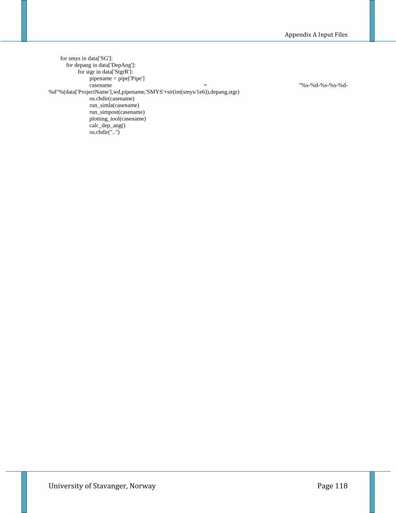
A.2 Run File ......................................................................................................................................... 117

A.3 Post Processing Input File (SIMPOST) ......................................................................................... 119

APPENDIX B OUTPUT FILES ................................................................................................................... 120

B.1 S-LAY ............................................................................................................................................ 121

B.1.1 Configuration ......................................................................................................................... 122

B.1.2 Required Top Tension ........................................................................................................... 123

B.1.3 Strain In The Overbend Region ............................................................................................. 125

B.1.4 Bending Moment at The Sagbend Region ............................................................................ 126

B.2 J-Lay 127

B.2.1 Configuration ......................................................................................................................... 128

B.2.2 Required Top Tension ........................................................................................................... 129

B.2.3 Strain In The Sagbend Region .............................................................................................. 131

B.2.4 Bending Moment at The Sagbend Region ............................................................................ 132

APPENDIX C CALCULATIONS ................................................................................................................ 133

C.1 Local Buckling (System Collapse Calculation) in the Overbend Area – DCC Check ................... 134

C.2 Local Buckling (System Collapse Calculation) in the Sagbend Area – LCC Check ..................... 142

C.3 Propagation Buckling .................................................................................................................... 151

C.4 On-Bottom Stability Calculation..................................................................................................... 155

C.5 Catenary Calculation ..................................................................................................................... 158

APPENDIX D SUMMARY OF ANALYSIS RESULTS ................................................................................ 161

D.1 14 Inch Pipe Diameter Results ...................................................................................................... 162




List of Tables

University of Stavanger, Norway vi

List of Tables

Table 3-1: Load Effect Factors and Load Combinations, Ref [12] ........................................................ 30

Table 3-2: Condition Load Effect Factors, Ref[12] ................................................................................ 30

Table 3-3: Material Resistance Factor, Ref [12] ................................................................................... 31

Table 3-4: Safety Class Definition, Ref [12] .......................................................................................... 31

Table 3-5: API Material Grades, Ref [12] .............................................................................................. 31

Table 3-6: API Material Strength Factor, 𝜶𝒖, Ref [12] .......................................................................... 32

Table 3-7: Maximum Fabrication Factor, Ref [12]................................................................................. 33

Table 3-8: Simplified Criteria for Overbend, Ref [12] ............................................................................ 39

Table 4-1: Material Parameter .............................................................................................................. 46

Table 4-2: Material Properties ............................................................................................................... 47

Table 4-3: S-Lay Vessel Data ............................................................................................................... 47

Table 4-4: J-Lay Vessel Data ................................................................................................................ 48

Table 4-5: Stinger Radius vs Departure Angle ..................................................................................... 49

Table 5-1: Wall Thickness (mm) Based on Local Buckling (System Collapse) .................................... 62

Table 5-2: Wall Thickness Based on Stability Criteria .......................................................................... 62

Table 5-3: Wall Thickness (mm) Based on Buckle Propagation ........................................................... 63

Table 5-4: Wall Thickness Summary (mm) ........................................................................................... 64

Table 5-5: 14 Inch X65 Wall Thickness (mm) vs Ovality ...................................................................... 69




Table 5-9: 14” Pipe S-Lay Result (X65) ................................................................................................ 76

Table 5-10: 14” Pipe J-Lay Result (X65) ............................................................................................... 77

Table 5-11: 20” Pipe S-Lay Result (X65) .............................................................................................. 78






Table 5-17: Effect of Increasing Allowable Strain In Overbend (14” Pipe Diameter)............................ 89




Table 5-21: Effect of Reducing the Stinger Length (14” Pipe Diameter) .............................................. 96


List of Tables

University of Stavanger, Norway vii


Table 5-24: Comparison Results for the S-Lay Method ...................................................................... 100

Table 5-25: Comparison Results fot the J-Lay Method ...................................................................... 101

List of Figures

University of Stavanger, Norway viii

List of Figures Figure 1-1 : Pieter Schelte Vessel, Ref [1] .................................................................................................... 1

Figure 2-1: Schematic of Saipem’s Castoro Sei Semi-Submersible S-Lay Vessel, Ref [21] ................. 5

Figure 2-2: Pipe Laying Configuration Using the S-Lay Method, Ref [3] ................................................ 6

Figure 2-3: Buckling during S-Lay, Ref [21] ............................................................................................ 7

Figure 2-4: Schematic Representation of S-Lay Pipeline Installation and Associate Pipeline Loadings, Ref [21] .................................................................................................................................................... 7

Figure 2-5: Schematic representation of J-lay pipeline installation and associated pipeline loading, Ref [21] .................................................................................................................................................. 10

Figure 2-6: Installation Equipment on S-7000, Ref [21] ........................................................................ 12

Figure 2-7: Comparison Tension for S-Lay and J-Lay Configurations, Ref [21] ................................... 13

Figure 2-8 : The hanging chain, the catenary, Ref [13] ........................................................................ 14

Figure 2-9 : The hanging chain, the catenary, Ref [13] ........................................................................ 14

Figure 2-10: Stress and Strain Diagram ............................................................................................... 22

Figure 2-11: Flow Chart of Strain Based Design, Ref ........................................................................... 23

Figure 2-12: Reference for Plastic Strain Calculation, Ref dnv ............................................................ 24

Figure 2-13: Moments as the Pipeline Passes Rollers on the Stinger, Ref rodringer .......................... 25

Figure 2-14: Typical Moment – Bending Curvature Diagram, Ref rodringer ........................................ 25

Figure 2-15: Moments and Strains in the Pipeline from the Stinger to the Seabed, Ref ...................... 26

Figure 3-1 : De-rating Values for Yield Stress of C-Mn and Duplex Stainless Steel,Ref [12] .............. 32

Figure 3-2 : Ovalizationduring Bending,Ref [21] ................................................................................... 34

Figure 3-3 : Three Types of Buckle Arrestors,Ref [21] ......................................................................... 38

Figure 3-4 : Wall Thickness Design Flowchart, Ref .............................................................................. 43

Figure 3-5 : Pipeline Installation Analysis Flowchart ............................................................................ 44

Figure 4-1 : Stinger Radius vs Departure Angle ................................................................................... 50

Figure 4-2 : Global Coordinate System in SIMLA, Ref [34] .................................................................. 51

Figure 4-3 : Local Coordinate System in SIMLA, Ref [34] .................................................................... 52

Figure 4-4 : Purpose and Communication between Modules in SIMLA, Ref [34] ................................ 52

Figure 4-5 : FlexEdit View ..................................................................................................................... 53

Figure 4-6 : Example of Run Operator in SIMLA using Python ............................................................ 53

Figure 4-7 : Example of XPOST View ................................................................................................... 54

Figure 4-8 : Example of Simvis View .................................................................................................... 54

Figure 4-9 : Example of Result Visualization using Matrix Plot ............................................................ 55

Figure 4-10 : S-Lay Model ..................................................................................................................... 55

Figure 4-11 : Example of a Route ......................................................................................................... 56

Figure 4-12 : Roller Configurations ....................................................................................................... 57

Figure 4-13 : Roller Configurations with Various Departure Angle for 120 m Stinger Length .............. 58

List of Figures

University of Stavanger, Norway ix

Figure 4-14 : J-Lay Model ..................................................................................................................... 59

Figure 5-1 : Wall Thickness for Various for Various Limit States (X65) ................................................ 65

Figure 5-2 : Wall Thickness as Function of Steel Grades (14 Inch Diameter) ...................................... 67




Figure 5-6 : 14 Inch X65 Wall Thickness (mm) vs Ovality .................................................................... 71




Figure 5-10 : Required Top Tension as Function of Water Depth for S-Lay X65 ................................. 74

Figure 5-11 : Required Top Tension as Function of Water Depth for J-Lay X65 ................................. 75

Figure 5-12 : S-Lay and J-Lay Required Top Tension as Function of Water Depth (14”X65) ............. 76








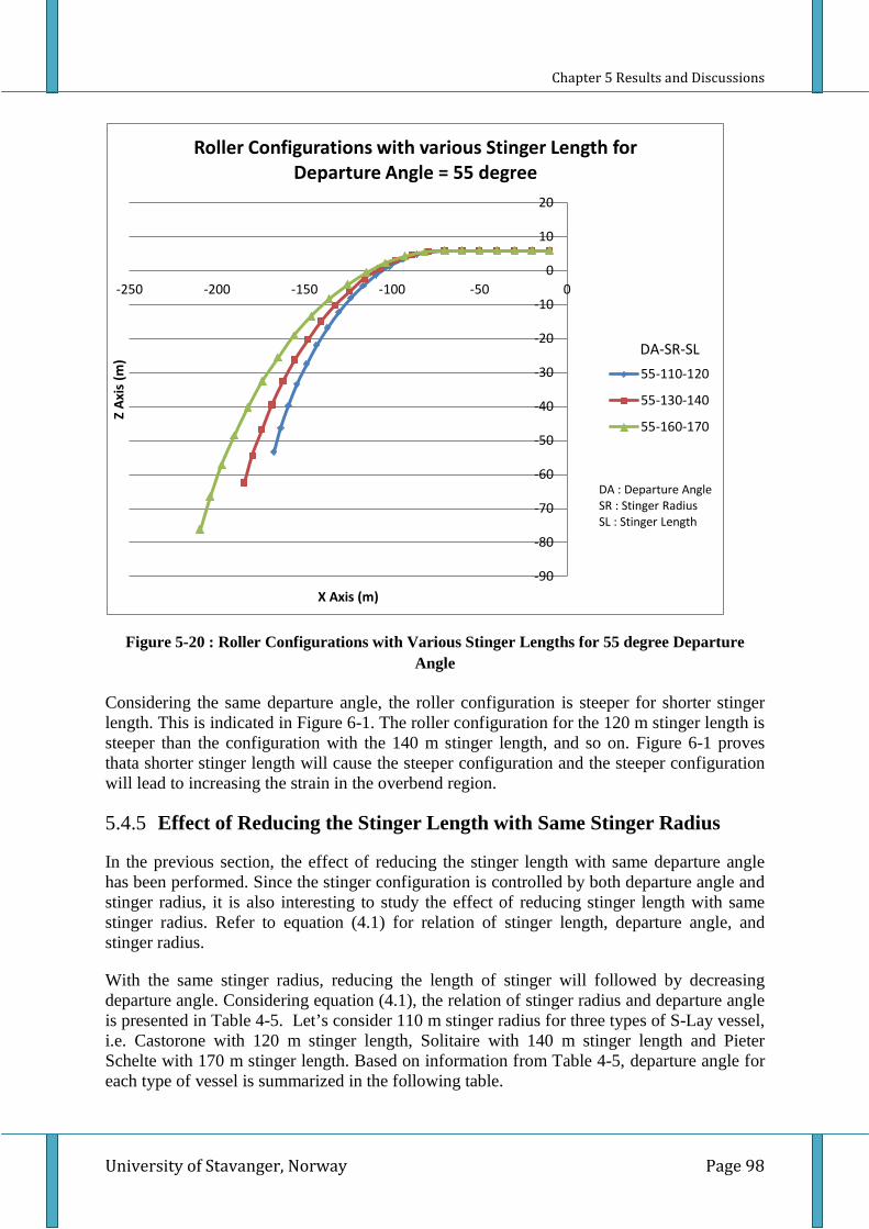
Figure 5-20 : Roller Configurations with Various Stinger Lengths for 55 degree Departure Angle ...... 98

Nomenclature

University of Stavanger, Norway x

Nomenclature

Symbols

Latin characters

b Pipe buoyancy per unit length

D Outer diameter of the pipe, unless specified otherwise

E Modulus of elasticity of the pipe steel, Young’s Modulus

fo Ovality (out-of-roundness)

fu Tensile strength

fy Yield stress

g Gravity acceleration

Ic Cross sectional moment of inertia of the steel pipe

κ Pipe curvature

M Bending moment

Mp Plastic moment capacity

MSd Design moment

M’Sd Normalized moment (MSd/Mp)

My Pipe bending moment at the nominal yield stress; My = 2σy Ic / D

n Hardening parameter

pc Characteristic collapse pressure

pe External pressure

pel Elastic collapse pressure

pi Internal pressure

pp Plastic collapse pressure

ppr Propagating pressure

ppr,BA Propagating buckle capacity of an infinite arrestor

pX Crossover pressure

Nomenclature

University of Stavanger, Norway xi

pmin Minimum internal pressure that can be sustained

Sp Plastic axial tension capacity

SSd Design effective axial force

S’Sd Normalized effective force (SSd/Sp)

T Tension

t Nominal pipe wall thickness (un-corroded)

t1 Characteristic wall thickness; t-tfab prior to operation. t shall be replaced with t1 due to possible failure where low capacity- system effects are present

t2 Characteristic wall thickness; t for pipelines prior to installation

tfab Fabrication thickness tolerance

Uc Mean current velocity normal to the pipe

ws Pipe submerged weight per unit length

Greek characters

αfab Fabrication factor

αu Material strength factor

β Factor used in combined loading criteria

γc Condition load effect factor

γm Material resistance factor

γsc Safety class resistance factor

γw Safety factor for on-bottom-stability

ε Strain

θ Liftoff angle

μ Friction coefficient

ν Poisson’s ratio

ρw Mass density of water

σy Nominal yield stress of the pipe steel

Nomenclature

University of Stavanger, Norway xii

Abbreviations

ALS Accidental Limit State

CP Cathodic Protection

CRA Corrosion Resistant Alloy

CTOD Crack Tip Opening Displacement

CWC Concrete Weight Coating

DNV Det Norske Veritas

DP Dynamic Positioning

ECA Engineering Critical Assessment

FLS Fatigue Limit State

GPS Global Positioning System

LC Load Controlled

LRFD Load and Resistance Factor Design

SMTS Specified Minimum Tensile Strength

SMYS Specified Minimum Yield Strength

ULS Ultimate Limit State

UOE Pipe fabrication process for welded pipes

UO Pipe fabrication process for welded pipes

TRB Three Roll Bending

ERW Electric Resistance Welding

Chapter 1 Introduction

University of Stavanger, Norway Page 1

CHAPTER 1 INTRODUCTION

1.1 Background Pipelines are major components of the oil and gas production. Both technical and economical challenges should be taken into considerations for pipeline design installations in ultra-deep water.

Pipeline installation methods and selection of pipeline concept are important concerns and set limitations to how deep a pipeline can be laid. Not only limitations to laying vessel tension capacity but also to technical design solutions are important in order to make pipeline installations and operations feasible in deep water depths.

Nowadays, projects have been completed and planned in water depths from more than 2000 meters up to 3500 meters and more. Some examples of deepwater pipeline projects are Medgaz project across Mediterranean Sea that has installed 24 inch pipelines at depths of 2155 meters and Blue Stream project with 24 inch pipeline at depths of 2150 m across the Black Sea. The deepest pipeline project, South Stream has been started in December 2012 in water depths more than 2200 m in the Black Sea, but this water depth record will not last long. A gas pipeline project between Oman and India have for long had plans of installing pipelines at depths of nearly 3500 meters in a 1100 km long crossing of the Arabian Sea to transmit gas from Middle East to India.

In this thesis, the possibilities for pipeline installation in water depths up to 4000 m using pipelay vessels with the biggest tension capacity will be studied. The Allseas Company has decided to build this vessel. This vessel, Pieter Schelte, has topside lift capacity of 48000 t, jacket lift capacity of 25000 t and pipelay tension capacity around 2000 t. This tension capacity will be doubling the capacity of Allseas’ Solitaire. Pieter Schelte is supposed to be ready for offshore operations in early 2014.

Figure 1-1 : Pieter Schelte Vessel, Ref [1]



1.2 Problem Statement A marine pipeline is exposed to different loads during installation such as tension, bending, and high external hydrostatic pressures which are becoming greater problems with increasing water depths. The tension applied in the pipe controls the sag-bend curvature while over-bend curvature is controlled by the stinger radius. The required tension depends on water depth, weight of the pipe, acceptable radius of curvature at the over-bend and acceptable stress at the sag-bend. The requirements to the large tension capacity may exceed the capacity of the most powerful S-Lay vessel in combination of very deep waters and thick walled pipes.

Accepting a higher working factor for the pipelines as well as using high steel grade steels will decrease the required wall thicknesses. These conditions lead to a reduction of pipeline weights and can therefore increase the water depth limits for the S-lay method. Some studies to support the idea to exceeding elastic proportionality for stress-strain behavior in the over-bend have been done. However, to extend the achievable water depth by increasing the allowable curvature in the over-bend may cause some crucial issues. Some lay variables such as lay pull, roller reaction, dynamic excitation from vessel motions and hydrodynamic loads need to be investigated. In addition further efforts to predict the historical pipe responses in non-linear behavior must be studied before allowing permanent deformations after installation.

The J-Lay method is another alternative to install pipelines in deeper water depths and larger diameters. In the J-Lay method, the requirements of curvature in the over-bend can be reduced; therefore only a short stinger is required to withstand the load from the lay span and to assist the pipe coming out from the vessel. The requirements of horizontal tension are smaller compared to the S-Lay method, only simply to withstand the submerged weight of the pipes, to control stresses, and to maintain a satisfactory curvature in the sag-bend. However, the J-Lay method does not allow more than one welding and NDT station, causing the welding process to be much slower than the S-Lay method. In addition, the availability of welding and NDT technology for thick pipes may aggravate this situation.

A very long free span of pipe sections from the barge to the seafloor is exposed to loads caused by vessel responses and vortex shedding due to marine currents in ultra deep waters. In fact, severe currents may cause vibrations and involve high Eigen-modes, therefore high dynamic stresses may happen as consequences. This phenomena combined with long time required for a pipe to reach the sea bottom can accumulate intolerable fatigue damage during installations, causing very small or even no margin for the on-bottom operating life.

1.3 Purpose and Scope The purpose of this thesis is to study the possibilities of pipeline installations in water depth up to 4000 m using pipelay vessel with the biggest tension capacity available and using appropriate technical solutions. This tension capacity will be 2000 t and the vessel will be ready for offshore operations in early 2014.



Scope of this thesis:

• Comprises development of 14 inch, 20 inch, 28 inch, and 30 inch steel pipelines for installation at water depths 800 m, 1300 m, 2000 m, 2500 m, 3000 m, 3500 m, and 4000 m;

• Comparison between the S-Lay and J-Lay methods for various pipeline sizes and water depths as mentioned above;

• Identify main challenges for pipeline installations in ultra deep water;

• Perform analysis for pipeline installation using software SIMLA and compare the results with ORCAFLEX, OFFPIPE, and manual calculations;

• Study the effect wall thickness requirements using the higher steel grades (X65, X70, X80, X100) for the case of combination of bending and external pressure;

• Study the effect of plastic strains in the over bend;

• Study the effect of changing in ovality;

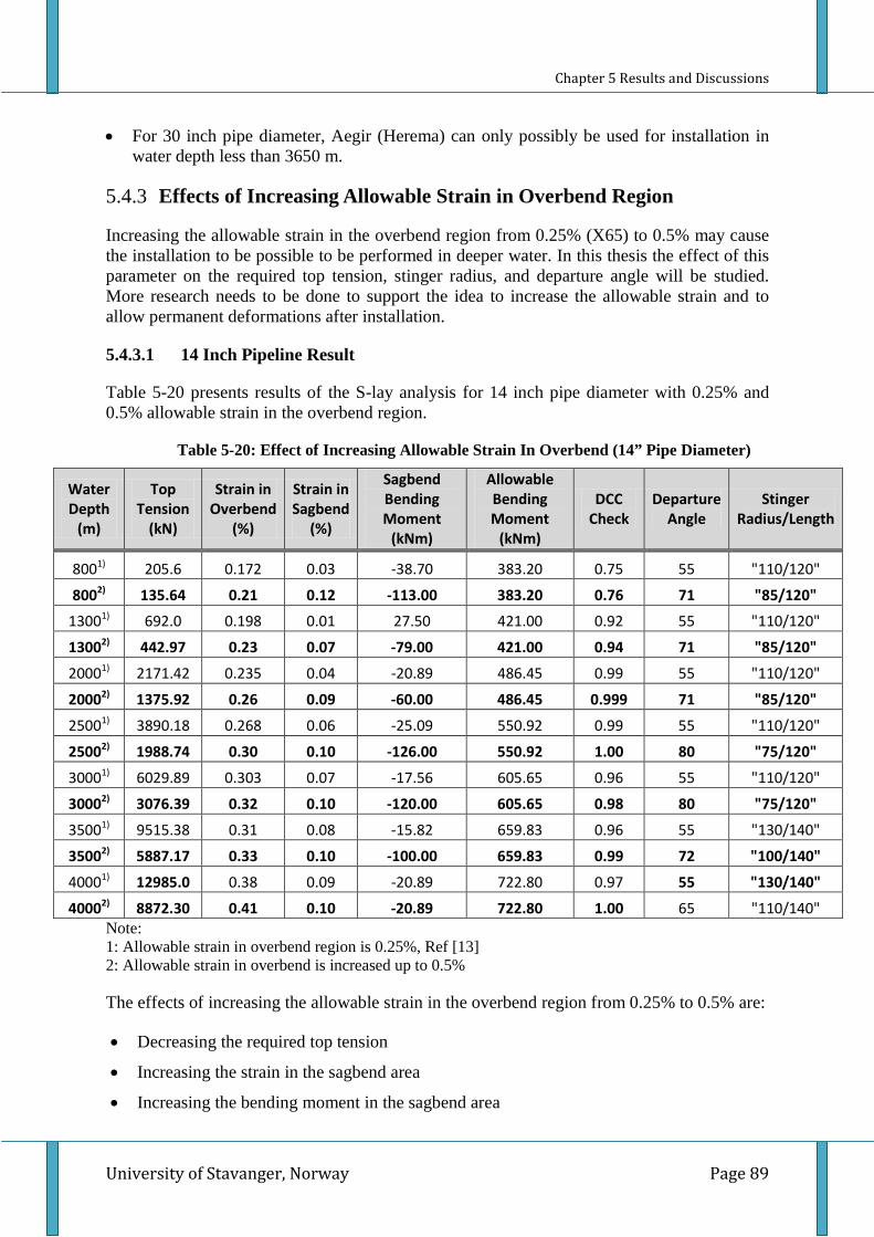
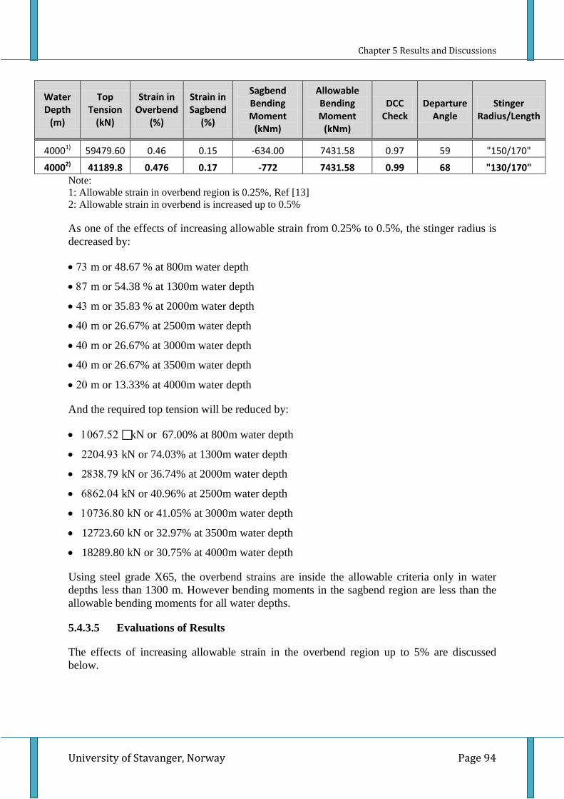
• Study the effect of increasing of allowable strain in overbent up to 0.5%;

• Study the effect of reducing the length of stinger.

1.4 Thesis Organization The remaining chapters in this thesis are organized as follows:

Chapter 2 (Basic Theory) presents the pipeline laying methods relevant for deep waters and discusses the main challenges related to developments of pipeline concepts at these water depths. The chapter also presents a discussion of the advantages and disadvantages of the different concepts. In addition, theoretical studies about pipe material and possibilities to exceed the elastic proportionality for stress-strain behavior are included in this chapter to establish a layable and operative pipeline at deep waters.

Chapter 3 (Design Criteria &Methodology) presents the design criteria for the pipelines being studied as part of the case studies, including pipeline properties, material data, data about the physical environmental and design criteria, as well as design methodology applied in the thesis.

Chapter 4 (Analysis Study) presents the S-Lay and J-Lay analysis for various water depths and pipeline sizes. The pipe laying systems modeled with the finite element software SIMLA, is explained.

Chapter 5 (Results and Discussions) presents results and evaluations regarding pipe layability studies of S-lay and J-lay methods in water depths up to 4000 m. The results and discussions of sensitivity studies such as the effect of changing in ovality, the effect of increasing material grade, the effect of increasing allowable strain in the overbend region and the effect



of reducing the length of stinger are also presented. In addition in this chapter, SIMLA results are compared to corresponding results obtained from OFFPIPE, ORCAFLEX and manual callculations.

Chapter 6 (Conclusion and Further Studies) presents conclusions and recommendations for further studies.

Chapter 2 Basic Theory


CHAPTER 2 BASIC THEORY

2.1 Pipeline Installation Pipeline installation is one of the most challenging offshore operations. A high level of engineering design is required to determine the required diameter of pipe, type of material, and installation method that are suitable for certain locations. Furthermore these criteria will be used for choosing installation vessel and determine the estimated cost.

This chapter outlines two common methods used to install pipeline, i.e:

• S-lay;

• J-lay.

2.1.1 S-Lay Method

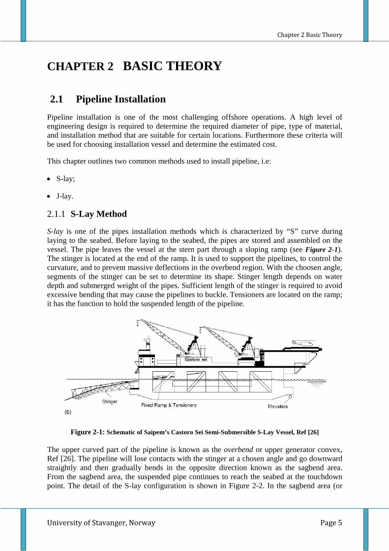
S-lay is one of the pipes installation methods which is characterized by “S” curve during laying to the seabed. Before laying to the seabed, the pipes are stored and assembled on the vessel. The pipe leaves the vessel at the stern part through a sloping ramp (see Figure 2-1). The stinger is located at the end of the ramp. It is used to support the pipelines, to control the curvature, and to prevent massive deflections in the overbend region. With the choosen angle, segments of the stinger can be set to determine its shape. Stinger length depends on water depth and submerged weight of the pipes. Sufficient length of the stinger is required to avoid excessive bending that may cause the pipelines to buckle. Tensioners are located on the ramp; it has the function to hold the suspended length of the pipeline.

Figure 2-1: Schematic of Saipem’s Castoro Sei Semi-Submersible S-Lay Vessel, Ref [26]

The upper curved part of the pipeline is known as the overbend or upper generator convex, Ref [26]. The pipeline will lose contacts with the stinger at a chosen angle and go downward straightly and then gradually bends in the opposite direction known as the sagbend area. From the sagbend area, the suspended pipe continues to reach the seabed at the touchdown point. The detail of the S-lay configuration is shown in Figure 2-2. In the sagbend area (or



known also as lower generator concave), the combination of bending and pressure loads are must safely be sustained.

The tension applied at the top is used to control the curvature in the sagbend region. Excessive bending, local buckling and collapse could happen if the tension in the top is lost due to sudden movements of the ship or any others reasons. A schematic showing initial buckle propagation from local collapse during S-Lay installation is presented in Figure 2-3.

The main function of the lay vessel is to provide tension to holds the suspended line pipes and to control its shape. The behavior of the long suspended pipeline is more like a cable rather than a beam. The water depth will determine the length of pipe, the tension required, as well as the curvature in the sagbend area. The deeper water, the bigger tension is required and this comes at a significant cost to the operations by requiring a modern installation vessel, Figure 2-4.

The objectives of installation design are:

• To avoid buckling failures in the overbend and the sagbend area;

• To keep the pipeline in the elastic regime.

Figure 2-2: Pipe Laying Configuration Using the S-Lay Method, Ref [4]



Figure 2-3: Buckling during S-Lay, Ref [26]

Figure 2-4: Schematic Representation of S-Lay Pipeline Installation and Associate Pipeline Loadings, Ref [26]

Some concerns for S-Lay method are the allowable strain in the overbend and the allowable bending moments in the sagbend region. The important parameters that control the maximum strain and maximum bending moment in the pipeline during installation are stinger length, stinger radius, tensioning capacity, and longitudinal trim of the vessel, Ref [18]. These parameters will control water depth at which a given pipeline can be laid.



Advantages

• The vessels have capability to instal pipelines with various diameters. No limitations to pipeline diameter and length;

• Minimum on-shore support required after the installation has begun;

• With the S-Lay method, some tasks such as welding, inspections, and field joint applications can be performed at the same time;

• Some contractors have good experiences with S-Lay method which is good for technical and economical aspects;

• Laying speed is quite high, even for large diameter pipelines, typically around 2 to 6 km/day, Ref [18]. The laying rate depends on seabed topography and waterdepth.

Disadvantages

• Limited installation depth due to limited vessel tension capacity;

• Long stinger is susceptible to hydrodynamic forces;

• Require clamping to pull the pipeline that can necessitate a heavy mooring system and high risk associated with a very long stinger subject to hydrodynamic forces. In addition, these options also could destroy the pipe coating;

• High probability of exceeding allowable strain in overbend area.

2.1.1.1 S- Lay Main Installation Component

Typically, S-Lay method is done by the following main installation equipments.

Tensioners

Tensioners are normally located close to the stern. The friction between rubber pads in the tensioning machines gives a tension on the pipe to control the curvature during laying down and to securing the integrity of the pipe. The required tension depends on water depth, length of the stinger, stinger radius, pipe size and weight. As the length and weight increase with increasing water depth, the required tension also increases. The tension capacity of the installation vessel will set a limitation to how deep the pipeline can be laid.

Transfer of tension between tensioner device and pipe is the most critical issue for some pipelay techniques, Ref [37]. The three methods for transfer of tension are:

• Long tensioners and low squeeze;

• Short tensioners and high squeeze;

• Shoulders with collars on the pipe.

The pipe coating area that is exposed to friction must be large enough in order to avoid damage; large tensioners with low squeeze can be used for this purpose.



In order to increase the possibility of pipeline installation in deeper water, tensioners can be applied after the overbend section. The benefit of this method is that lower strain will occur in the overbend areasince the combination of the tensioner force and bending effect can be avoided, Ref [37].

Stinger

The stinger is a frame structure with roller to support the pipelines during installation and create the pipe’s curvature in the overbend area. Typically, some hinged members are built in the stinger to adjust the stinger curvature. Different type of vessels has different length of stinger, but for installation vessels in deepwater the length could be more than 100 m. For example Solitaire has a 140 m stinger length and the new S-lay vessel, Pieter Schelte has 170 m stinger length. In deeper water, a longer stinger length is required to maintain the strain less than the maximum acceptable limit criteria for the overbend section. Using short stinger can cause higher bending and pipeline damage during pipeline installation. The stinger should be able to withstand all the forces acting during operation, such as:

• Hydrodynamic forces due to waves and currents;

• Load from laying the pipeline;

• The stinger self weight;

• Load acting on the stinger due to vessel movements.

There are two types of stinger configurations that commonly used nowadays:

• Rigid stingers

This type of stinger have fixed configuration with certain length and an un-adjustable angle of curvature. The stinger is connected rigidly to the vessel, restricted to small movements only.

• Articulated stingers joined by hinges

Since this stinger uses hinge joints in each segment, the angle of its curvature radius can be adjusted as per required. An articulated stinger is more flexible for pipeline installation in deeper water by setting the curvature angle close to a vertical position. With this vertical position, the free span length can be reduced and furthermore this can decrease the stresses on the pipelines.

2.1.2 J-Lay Method

The suspended pipe length increases in deeper water conditions, and as a result an increasing tension requirement can not be avoided. This tough requirement is solved with the J-Lay method. This method is characterized by the pipeline leaving the vessel from nearly a vertical position and has J-shape on the way down to the sea floor. In the J-Lay method, the requirement to curvature in the over-bend can be reduced; therefore only a short stinger is required to withstand the load from the lay span. The horizontal tension required is smaller compared to the S-Lay method; its role is only simply to withstand the submerged weight of the pipes, to control stresses, and to maintain a satisfactory curvature in the sag-bend. In



addition, the shorter suspended length in the J-Lay method can cause a significant reductions in the thruster power requirements.

However, due to the near vertical installation, the J-Lay method does not allow more than one welding and NDT station. To solve these limitations, longer pipe section are prepared to increase the efficiency of the operation. For this purpose, around four to six 12 m sections are welded on shore. After inspection, coating and the welding proceses, the long section of the pipe is lowered to sea bottom. Because of these aspects, the J-lay method has a slow production rate and the availability of welding and NDT technology for thick pipes may aggravate this situation.

In the J-Lay method, the pipeline must be designed to withstand the load condition that is illustrated schematically in Figure 2-5. From this figure, we can see that the pipe is exposed to high tension and reatively small external pressure in the surface area, and further down, the pressure increases and the tension decreases progresively. Furthermore, a propagation buckle also needs to be taken into considerations and it is necessary to install buckle arrestors to eliminate this problem.

Figure 2-5: Schematic representation of J-lay pipeline installation and associated pipeline loading, Ref [26]

Advantages

• The required tension can be reduced as the pipe leaves the vessel near to vertical position. The tensionis only required to maintain bending at acceptable criteria for the sagbend region;

• No stingeris required. No overbend, therefore the limit criteria for this region can be eliminated;



• The free span is shorter compared to S-Lay method because lower lay tensions are resulting in reduced bottom tension in the pipe;

• Compared to S-Lay method, the J-lay method pipeline laying is more accurate because the location of the touchdown point is near to the vessel;

• Less vulnerable to the weather conditions due to a decreased area of interaction with the waves. Only a short length of the line close to the surface is exposed to wave motions because the pipelines are installed nearly atvertical position;

• Fast and relatively safe abandonment and recovery turn around.

Disadvantages

• The J-Lay method does not allow more than one welding and NDT station, causing the welding process to be much slower than the S-Lay method. In addition, the availability of welding and NDT technology for thick pipes may aggravate this situation;

• The effect of the weight and the height of the tower are needed to be taken into consideration for stability issues;

• The method is not suitable for installation in shallow water. In shallow water the pipe bend at the seafloor will be too sharp and cause pipeline damage;

• The capability of the J-Lay method in deep and very deep waters requires barges with dynamic positioning capabilities.

2.1.2.1 J-Lay Main Installation Equipment

Typically, the J-Lay method is carried out by the following main installation equipment:

Towers

The tower is a nearly vertical frame that supports the pipeline during J-Lay operations and consists of tensioners and work stations. The tower’s orientation is normally between 0o and 15o relative to the vertical position. The location of J-Lay towers is close to the middle of the vessel for the DB 50 (McDermott’s) or at the stern for S-7000 (Saipem), as shown in Figure 2-6, Ref [21].

Tensioners

For the J-Lay method, sufficient tension must be provided by the tensioner to avoid buckling in the sagbend area during installation. The submerged weight controls the required tension and the tension controls the curvature in the sagbend region. Some methods have been adopted by the J-Lay vessel owners to maintain a high tension. For example S-7000 has 525 t tension capacity using friction claps. Another system has been used by the Balder vessel to get 1050 t capacity. This system uses a collar that is welded to the upper end of the pipe and is held by the clamp at the end of the tower.



Figure 2-6: Installation Equipment on S-7000, Ref [26]

2.1.3 Comparison between S-Lay and J-Lay

Different pipelay configurations will cause different required top tension and critical area. For example, the required top tension for S-lay configuration is higher compared to J-Lay configuration. The critical area that becomes most concern for J-Lay configuration is the sagbend region while for S-Lay, the overbend region will become more critical than the sagbend. In the overbend region, the strain should satisfy the criteria stated in DNV-OS-F101 (2007). And for J-Lay, bending moment in the sagbend area should be less than allowable bending moments for appropriate water depth.

Comparison of S-Lay and J-Lay configuration is shown in Figure 2-7. Let’s consider two pipelines with same properties and same liftoff angles being installed using S-Lay and J-lay method respectively. In these cases, the differences of required top tension for both methods can be calculated.



Figure 2-7: Comparison Tension for S-Lay and J-Lay Configurations, Ref [26]

Based on Figure 2-7, using static equilibrium method, the horizontal and vertical forces can be found:

𝐻 = 𝑇 cos 𝜃 (2.1)

𝑉 = 𝑇 sin 𝜃 (2.2)

And the required top tension is:

𝑇 = √𝐻2 + 𝑉2 (2.3)

Since the submerged weight “ws” is known based on pipe diameter and thickness, and the suspended length of pipe “s” is also known, the vertical tension can be calculated using the following formula:

𝑉 = 𝑤𝑠𝑠 (2.4)

In the J-Lay case, horizontal forces “H” is only required to counteract horizontal tension at the touchdown point “𝐻𝑜". And for the S-Lay case, the horizontal forces are required to counteract the combination of horizontal tension at touchdown point "𝐻𝑜" and the horizontal component of stinger reaction forces “𝑆𝐻". Therefore, since the horizontal forces for the S-Lay method are higher than for the J-Lay method, the required top tension for S-Lay is also higher than for J-Lay.



2.2 Catenary Analysis The objective of introducing the catenary equation is to provide a validation of the model developed in this master thesis. The equation for the catenary is derived in this section.

Figure 2-8 : The hanging chain, the catenary, Ref [14]

Based on information presented in Figure 2-8, the relation for distance to touchdown point “L”can be developed as follow:

Figure 2-9 : The hanging chain, the catenary, Ref [14]

𝑑𝑠 = �𝑑𝑥2 + 𝑑𝑦2

𝑑𝑦𝑑𝑥

=𝑉𝐻

𝑉 = 𝐻𝑑𝑦𝑑𝑥

𝑑𝑉𝑑𝑥

= 𝐻𝑑2𝑦𝑑𝑥2

x

y

H

H

V T

L

h s

H

dx

H V

T

dy ds



And

𝑑𝑉 = 𝑤𝑠𝑑𝑠

𝑑𝑉𝑑𝑥

= 𝑤𝑠𝑑𝑠𝑑𝑥

Then :

𝑑𝑉𝑑𝑥

= 𝑤𝑠𝑑𝑠𝑑𝑥


𝑤𝑠�𝑑𝑥2 + 𝑑𝑦2 = 𝐻𝑑2𝑦𝑑𝑥2

𝑑𝑥

𝑤𝑠𝑑𝑥�1 + �𝑑𝑦𝑑𝑥�2


𝑑𝑥

𝑤𝑠𝐻𝑑𝑥 =

𝑑2𝑦𝑑𝑥2

�1 + �𝑑𝑦𝑑𝑥�2𝑑𝑥

𝑤𝑠𝐻𝑑𝑥 =

𝑑𝑑𝑥�𝑑𝑦𝑑𝑥�

�1 + �𝑑𝑦𝑑𝑥�2𝑑𝑥

�𝑤𝑠𝐻𝑑𝑥

𝑥

0= �

𝑑(𝑦′)

�1 + (𝑦′)2𝑑𝑥

𝑦′

0

𝑤𝑠𝐻𝑥 = arcsinh (𝑦 ′)

𝑦 ′ = 𝑠𝑖𝑛ℎ �𝑤𝑠𝐻𝑥�

The formula for the caternary is:

𝑦 = 𝐻𝑤𝑠�𝑐𝑜𝑠ℎ 𝑤𝑠

𝐻𝑥 − 1� (2.5)

In terms of x = L and y = water depth h we have:

ℎ = 𝐻𝑤𝑠�𝑐𝑜𝑠ℎ 𝑤𝑠

𝐻𝐿 − 1� (2.6)

ℎ𝑤𝑠𝐻

+ 1 = 𝑐𝑜𝑠ℎ �𝑤𝑠𝐻𝐿�



𝑤𝑠𝐻𝐿 = 𝑎𝑟𝑐𝑐𝑜𝑠ℎ �

ℎ𝑤𝑠𝐻

+ 1�

Therefore:

𝐿 = 𝐻𝑤𝑠𝑎𝑟𝑐𝑐𝑜𝑠ℎ �ℎ𝑤𝑠

𝐻+ 1� (2.7)

From the previous page, we know that:

𝑤𝑠𝑑𝑠𝑑𝑥


𝑑𝑠𝑑𝑥

=𝐻𝑤𝑠

𝑑2𝑦𝑑𝑥2

𝑠 = 𝐻𝑤𝑠�𝑠𝑖𝑛ℎ 𝑤𝑠

𝐻𝐿� (2.8)

Using equation (2.6) and (2.8) we can develop the formula to get equation (2.9) :

𝑠2 − ℎ2 = �𝐻𝑤𝑠�2

�𝑠𝑖𝑛ℎ2 �𝑤𝑠𝐻𝐿� − �𝑐𝑜𝑠ℎ �

𝑤𝑠𝐻𝐿� − 1�

2�

𝑠2 − ℎ2 = �𝐻𝑤𝑠�2

�𝑠𝑖𝑛ℎ2 �𝑤𝑠𝐻𝐿� − �𝑐𝑜𝑠ℎ2 �

𝑤𝑠𝐻𝐿� − 2𝑐𝑜𝑠ℎ �

𝑤𝑠𝐻𝐿� + 1��

𝑠2 − ℎ2 = �𝐻𝑤𝑠�2

�𝑠𝑖𝑛ℎ2 �𝑤𝑠𝐻𝐿� − 𝑐𝑜𝑠ℎ2 �

𝑤𝑠𝐻𝐿� − 1 + 2𝑐𝑜𝑠ℎ �

𝑤𝑠𝐻𝐿��

We know that :

𝑠𝑖𝑛ℎ2𝛼 − 𝑐𝑜𝑠ℎ2𝛼 = −1

Hence :

𝑠2 − ℎ2 = �𝐻𝑤𝑠�2

�−1 − 1 + 2𝑐𝑜𝑠ℎ �𝑤𝑠𝐻𝐿��

𝑠2 − ℎ2 = �𝐻𝑤𝑠�2

�2𝑐𝑜𝑠ℎ �𝑤𝑠𝐻𝐿� − 2�

𝑠2 − ℎ2 = 2 �𝐻𝑤𝑠�2

�𝑐𝑜𝑠ℎ �𝑤𝑠𝐻𝐿� − 1�

𝑠2 − ℎ2 = 2𝐻𝑤𝑠

𝐻𝑤𝑠�𝑐𝑜𝑠ℎ �

𝑤𝑠𝐻𝐿� − 1�



𝑠2 − ℎ2 = 2𝐻𝑤𝑠ℎ

𝑤𝑠2ℎ

(𝑠2 − ℎ2) =𝑤𝑠2ℎ

2𝐻𝑤𝑠ℎ

And the equation for horizontal tension is :

𝐻 = 𝑤𝑠2ℎ

(𝑠2 − ℎ2) (2.9)

Therefore, the required top tension as found in the computer analysis can be compared with results of hand calculation using equation 2.9, equation 2.4 and equation 2.3.

The bending strain can be calculated with the following equation, Ref [32] :

𝜀 = 𝐷2𝑅

(2.10)

Where :

𝜀 Bending strain D Outer Pipe Diameter

R Bending radius of the pipeline

The minimum over-bend radius is given by the equation, Ref [32] :

𝑅 = 𝐸.𝐷2𝜎0𝐷𝐹

(2.11)

Where,

𝜎0 Minimum specified yield stress

DF Design factor, usually 0.85

E Elastic modulus of the pipeline

D Outside pipe steel diameter

According to equation (2.11) the bigger pipe diameter requires a larger stinger radius to avoid plastic deformation.

2.3 Pipe Material Material type is determined based on various factors such as:

• Water depth;

• External hydrostatic pressure;

• Internal pressure;

• Fluid characteristics;



• Environmental conditions;

• Weight requirements;

• Installation analysis;

• Seabed topography;

• Cost

According to DNV-OS-F101 (2007), the following material characteristics shall be considered:

• Mechanical properties; • Hardness; • Fracture toughness; • Fatigue resistance; • Weldability; • Corrosion resistance.

In order to ensure the compatibility of the pipeline, the following supplementary requirements are need to be identified in materials selection, Ref [13]:

1. Supplementary requirement S, sour service

A pipeline that transports fluid with hydrogen sulphide (H2S) contents shall be evaluated for ‘sour service’ according to ISO 15156. For materials specified for sour service in ISO 15156, specific hardness requirements always apply, Ref [13].

2. Supplementary requirement F, fracture arrest properties

Supplementary requirements to fracture arrest properties are given in Sec.7 I200 DNV-OS-F101 (2007) and are valid for gas pipelines carrying essentially pure methane up to 80% usage factor, up to a pressure of 15 MPa, 30 mm wall thickness and 1120 mm diameter, Ref [13].

For conditions beyond these limitations, the calculation reflecting the actual conditions or full-scale test should be considered to determine the required fracture arrest properties.

3. Supplementary requirement P, Plastic Deformation

According to DNV-OS-F101 (2007), supplementary requirement (P) is applicable to linepipe when the total nominal strain in any direction from a single event is exceeding 1.0% or accumulated nominal plastic strainis are exceeding 2.0%.

For pipes that require supplementary requirement (P), tensile testing should be carried out in the longitudinal direction to satisfy DNV requirements.



4. Supplementary requirement D, Dimensional Requirements

Requirements for tolerances should be selected considering the influence of dimensions and tolerances on the subsequent fabrication/installation activities and the welding facilities to be used, Ref [13].

5. Supplementary requirement U, Utilization

The Purchaser may in retrospect upgrade a pipe delivery to be in accordance with Supplementary requirement U. Incase of more than 50 test units it must be demonstrated that the actual average yield stress is at least two (2.0) standard deviations above the SMYS. If the number of test units is between 10 and 20 the actual average yield stress shall as a minimum be 2.3 standard deviations above SMYS, and 2.1 if the number oftest units are between 21 and 49, Ref [13].

2.3.1 Material Grade

The steel should strong enough to withstand transverse tensile and longitudinal forces during operation and installation. Besides that, the pipelines should also be constructed by materials with sufficient toughness to resist impact loads and to tolerate defects. Weldability is critical problem, it is important to make sure that the pipeline is possible to be welded with the same strength and toughness as the rest of the pipe, and also due to economical reasons, Ref [36].

The properties mentioned above are determinied by the steel grades. Different steel grades will have different strength and characteristics.

For pipeline design, steel grade X65, from API 5L (2004) are normally used. X70 steel grade has been used in offshore projects, i.e. for the planned Oman India Gas Pipeline project and the installed Medgaz pipeline at 2155 m water depth, Ref [10]. This project used 24 inch pipe diameter with constant internal diameter. Steel grades higher than X70 are only used in onshore project so far. There are around five onshore projects that are identified using X80 steel grade, i.e. Ref [6]:

• Germany, Mega II Pipeline (1985); • Czechoslovakia (1986); • Alberta Canada, Empress East Compressor Station (1990); • Germany Schlüchtern to Wetter, Ruhrgas (1993); • Alberta Canada, Mitzihwin Project (1994).

Higher grades are currently under active development. X100 grades are being actively developed by several companies, Ref [6].

Carbon Steel

The carbon steel pipelines are alloyed with various elements such as carbon, manganese, silicon, phosphorus and sulphur. For modern pipelines the amount of carbon are varying from 0.10% to 0.15%, between 0.80% and 1.60% manganese, under 0.40% silicon, less than 0.20% and 0.10% phosphorus and sulphur content, and under 0.5% copper, nickel and chromium, Ref [8]. The effect of alloying elements with certain composition into the steel



material will determine the steel grade, and hereby the strength, weldability, toughness and ductility of the pipe.

Increasing the material resistances to corrosions can be done by applying corrosion resistant materials such as martensitic stainless steels, duplex stainless steels, super duplex stainless steels, (super) austenitic stainless steels and nickel alloys. These are known as Corrosion Resistant Alloys (CRA). The CRA are used for internal corrosion resitence while Cathodic Protection (CP) and external coating are acting as external corrosion resistances. The CRA that is used in one location could be different from another location and depends on the type of transported fluid.

2.3.1.1 Advantages of High Strength Steel

The following lists are described the advantages of using high strength steel in pipeline industry.

1. Potential Cost Reduction

Higher wall thickness is required to withstand internal and external pressure especially in deep and ultra deep water conditions. Using high strength material grade can reduce the required wall thickness and can hereby increase the chance to reduce the overall cost of the project. This cost reduction due to decreasing of wall thickness can be achieved because of the pipe manufacturing and construction processes. Furthermore, some aspects such as transportation, welding consumables, welding equipment rental and overall lay time could possibly give contribution to reduce the cost.

Price (1993), Ref [39], considered both the direct and indirect consequences of using a high strength steel, and estimated a 7.5% overall project saving for a 42-inch offshore line laid with X80 instead of X65.

Using non standard pipeline diameter and thickness can also be considered as one of alternative solutions to reduce the cost. The optimum pipe diameter and thickness based on design calculation or modeling is more effective to be choosen instead of selecting the larger standard size.

2. Wall Thickness and Construction

As mentioned above, using higher steel grade will reduce the wall thickness requirement. Thinner wall thickness will reduce construction/lay time because a thinner wall requires less field welding. Further impact on reducing wall thickness is the lay barge requirement. This is related to weight of the pipe and availability of vessel with enough tension capacity.

3. Weldability

Higher wall thickness gives some difficulties related to weldability. The cooling rate of weld will increase for higher wall thickness. The increasing of the cooling rate causes potensial problems with hardness, fracture toughness, and cold cracking (if non-hydrogen controlled welding processes are used). In other words, the effect of increasing the material grade will reduce the cooling rate of the weld.



4. Pigging Requirements

It is required to have enough space for the pigging purpose especially in deep water developments. Some types of pigging tools will limit the possibility to use thicker wall thickness. Therefore, using thinner wall thickness as the impact of higher strength material will give advantages for pigging operations.

2.3.1.2 Disadvantages of High Strength Steel

The disadvantages of using high strength steel in the pipeline industry are:

1. Increase in material cost per volume

The higher strength material is more expensive than ordinary material grade. Therefore it is important to compare the increasing cost due to the increase in material grade with cost reductions due to decreasing in total required wall thickness.

2. Limited Suppliers

Using material grades above X70 represents challenges to the pipeline industry because of the limitations of proven suppliers available in the world.

3. Welding Restrictions

Welding to achieve the best quality may be takes some times due to some restriction and complex control for higher material grade. Besides that, limited experience of welding high material grade especially for offshore project also need to be considered if selecting higher material grade.

4. Limited Offshore Installation Capabilities

The limited number of pipelay installation contractor with proven experience of welding X70 represents another challenge to choose higher material grade.

5. Repair Problems

There is no experience for pipeline repair using hyperbaric welding for higher material grade so far. Therefore some studies are required in order to get better understanding of this issue. Another alternative to repair a pipeline is using the hot tap method, but same problem as with the first alternative is present; there is no experience for high strength material in offshore developments.

2.4 Plasticity during Installation Some studies to support the idea to exceeding elastic proportionality for stress-strain behavior in the over-bend have been done. In some circumstances, this can be done safely.

Strain based design is one method allowing the pipe to go beyond yield. The following lists are strain criteria based on DNV-OS-F101 (2007):



• Strain requirements - If total nominal strain ≤ 0.4 %, there is no additional requirement - If total nominal strain > 0.4 %, ECA should be implemented - If total nominal strain > 1.0 %, additional material tests, i.e. supplement requirement

P is required • Plastic Strain degrades the fracture resistance of material each time the pipe is yielded.

Additional material tests are also required if the accumulated plastic strain exceeds 2.0 %.

• Reeling requires ECA and additional testing.

Strain based design can be shown graphically in Figure 2-10.

Figure 2-10: Stress and Strain Diagram, Ref [20]

The process of strain based design is shown in the following flow chart, Figure 2-11.

% Strain

Stress Total strain

Plastic strain

Engineering Critical Assessment (ECA)

Additional Testing

SMYS

0.5 0.4 1



Figure 2-11: Flow Chart of Strain Based Design, Ref [20]

When the pipe yields plastically, the effect due to that strain will be cumulative. Permaent deformation will happen. If the total nominal longitudinal strain exceeds 0.4 % an engineering critical assessment (ECA) must be performed.

Furthermore, if the total nominal strain exceed 1.0 % or if the accumulated plastic strain more than 2 %, the additional requirements, i.e. supplementary requirement P need to be satisfied. This supplementary requirement determines the fracture toughness of the material and particularly the welds. Additional test need to be carried out. The tests include crack tip opening displacement (CTOD) on specimens of the weld. The test is based on the largest weld defects allowed by the welding specification.

With reeled pipe, the accumulated plastic strain always exceeds 2.0%. Usually, the accumulated plastic strain is close to 10%. But for the S-Lay and J-Lay method, it is very

START

Pressure Containment

Criteria

System Collapse Criteria

Load Controlled

Criteria Combined Loading

Displacement Controlled

Criteria

𝜺𝟏,𝒏𝒐𝒎≤ 𝟎.𝟒%

𝜺𝟏,𝒏𝒐𝒎> 1% 𝑜𝑟 𝜺𝒑> 2.0%

ECA on Installation Girth Welds

Supplementary Requirement P

FINISH

Yes

Yes

No

No

𝜀1,𝑛𝑜𝑚 = Total Nominal Longitudinal Strain

𝜀𝑝 = Accumulated Plastic Strain



rare to reach plastic limits. The reason is because the local buckling due to combination of external pressure and bending moment is happened before the plastic limit can be achieved.

2.4.1 Allowable Strain of a pipeline

Some experiences have proven that the steel pipeline is able to bend exceeding the yield stress without reducing the capacity to withstand internal pressure. These experiences can be seen in the reeling process where the strain can reach 2-3%. The yielding point for pipelines is defined as the stresses at which the total strain is 0.5%, Ref [34]. The total strain is a combination of elastic and plastic strain. Based on DNV OS F-101, the total strain of 0.5% for 415 grade C-Mn Steel consist of 0.2% elastic strain and 0.3% plastic strain, Ref [34].

Figure 2-12: Reference for Plastic Strain Calculation, Ref [13]

Normally the proportional limit for pipeline is about 75% yield stress and it is tolerated up to 85% the yield stress. Because of this, even in normal laying condition, it is normal if the pipeline experience plastic deformation. This is the reason that in practice it is common to base the criteria for dimensioning of laying parameters on accepted strains and not on stresses, Ref [34].

2.4.2 Special Strength Conditions during Pipeline Laying

In S-Lay method, the pipeline doesn’t contact directly to the stinger but will rest on some rollers. Because of this the friction force between the pipeline and the stinger is decreased and the bending moment will be highest in the roller positions and minimum in the mid span between two rollers. Figure 2-13 presents the moment diagram in the rollers position. The strain in the roller position might be exceed the proportional limit and causes plastic deformation on the pipeline.



Figure 2-13: Moments as the Pipeline Passes Rollers on the Stinger, Ref [34]

2.4.3 Exceeding the Bending Strength

High external pressure at pipelines which are installed in deep water, lead to the requirement of thicker wall thickness. ‘Thick walled pipelines’ terms is usually used for pipeline with less than 40-50 of diameter/wall thickness ratio. A ‘thick walled pipelines’ typical moment - curvature diagram is shown in Figure 2-14.

Figure 2-14: Typical Moment – Bending Curvature Diagram, Ref [34]

Figure above shows Re as the bending radius and 1/Re as bending curvature where the plastic deformation started. Ovalization will be occured to the pipelines’ cross section when the pipeline is bent even bigger. If it continues, the maximum moment (Mu ) will be reached with Ru as the correspond bending radius. The curvature of the pipeline capacity will be reached if the bending radius is further reduced with Rc as the correspond bending radius. Once this



degree of curvature achieved, local buckling will occur at the compressive side of the pipelines. For ‘thin wall thickness’ pipeline’s cross section with ratio of diameter / wall thickness greater than 250 to 300, the local buckling is happened in the elastic zone, Ref [34].

Curvature correspond to Rc does not always have to be larger than the curvature correspond to Ru. To avoid local buckling, the smallest curvature of these two should be considered, Ref [34].

The bending radius in overbend and sagbend are important to be kept large enough as this will increase the safety to avoid local bukcling , Ref [34].

2.4.4 Residual Curvature

Most of the time the pipeline will not rest on the seabed in perfectly flat condition due to surface unevenness, etc. The residual curvature after installation might be tolerated due to this uneven condition.

When laying on the seabed, the pipeline has axial force similar to installation horizontal tensile force. If there is residual curvature, this axial force will help to straighten the pipeline. Nevertheless, during pipeline repair operation, this axial force might cause some problems.

Theoretically, pipeline can be straightened using the bending forces in the sagbend if plastic deformation occurs in the overbend.

The relation of moment and strain in the pipeline from the stinger to the seabed that is experiencing plastic deformation is presented in Figure 2-15.

Figure 2-15: Moments and Strains in the Pipeline from the Stinger to the Seabed, Ref [34]

The figure above shows some residual curvature that is occured after the stinger location. A large moment added to the pipeline in the sagbend. The moment can help straighten the pipeline, however it also can create residual curvature in opposite direction if the value is very large.



A large ovalisation will result the reduction of pipeline structural capacity. At certain location/condition such as artificial supports, shoulders of free span and settlemet at support, the point load may accur. Furthermore, according to DNV, the ovalisation should be investigated for the point load on each section of the pipe.

Ovalisation issues can be reduced by increasing the pipeline wall thickness. Increasing the pipeline bending curvature will lead the increment of ovalisation more than proportionlaly. Some of the ovalisation will be in plastic if the curvature in plastic strain, which means that residual ovalisation will remain eventhough the stress has been removed. The maximum ovalisation for pipeline with a large wall thickness will be less than 0.5 to 1 % if the strains are less than 0.5 %; which means that the residual ovalisation is very small after stress has been removed Ref [34].

Large bending radius on the pipeline will cause ovalisation. Ovalisation is a condition when the pipeline cross section is not a perfect circle but will be flattened by some degree.

Chapter 3 Design Criteria and Methodology


CHAPTER 3 DESIGN CRITERIA AND METHODOLOGY

3.1 Design Codes The following standards and recommended practices should be applied for pipeline installation in deep water and ultra-deep water conditions:

• DNV-OS-F101 (2007) Submarine Pipeline Systems;

• DNV-RP-F109 (2007) On-bottom Stability Design of Submarine Pipelines.

3.2 Design Criteria

3.2.1 Loads Criteria

The purpose of categorizing the different loads is to give informations about the load effects and their uncertainties.

3.2.1.1 Functional Loads

Functional loads are loads that occur due to the physical characteristics of the pipeline system and its intended use.

According to DNV-OS-F101, Ref [13], the following phenomena are the minimum requirements that need to taken into considerations when establishing functional loads :

• Weight; • external hydrostatic pressure; • internal pressure; • temperature of contents; • pre-stressing; • reactions from components (flanges, clamps etc.); • permanent deformation of supporting structure; • cover (e.g. soil, rock, mattresses, culverts); • reaction from seabed (friction and rotational stiffness); • permanent deformations due to subsidence of ground, both vertical and horizontal; • permanent deformations due to frost heave; • changed axial friction due to freezing ; • Possible loads due to ice interference, e.g. bulb growth around buried pipelines near

fixed points (in-line valves/tees, fixed plants etc.), drifting ice etc; • loads induced by frequent pigging operations.



3.2.1.2 Environmental Loads

Environmental loads are the loads on the pipeline caused by the effects of surrounding environment and that are not otherwise specified as functional or accidental loads, such as:

• Static load, water pressure; • Wind loads; • Hydrodynamic loads including currents; • Ice loads.

3.2.2 Load Combinations

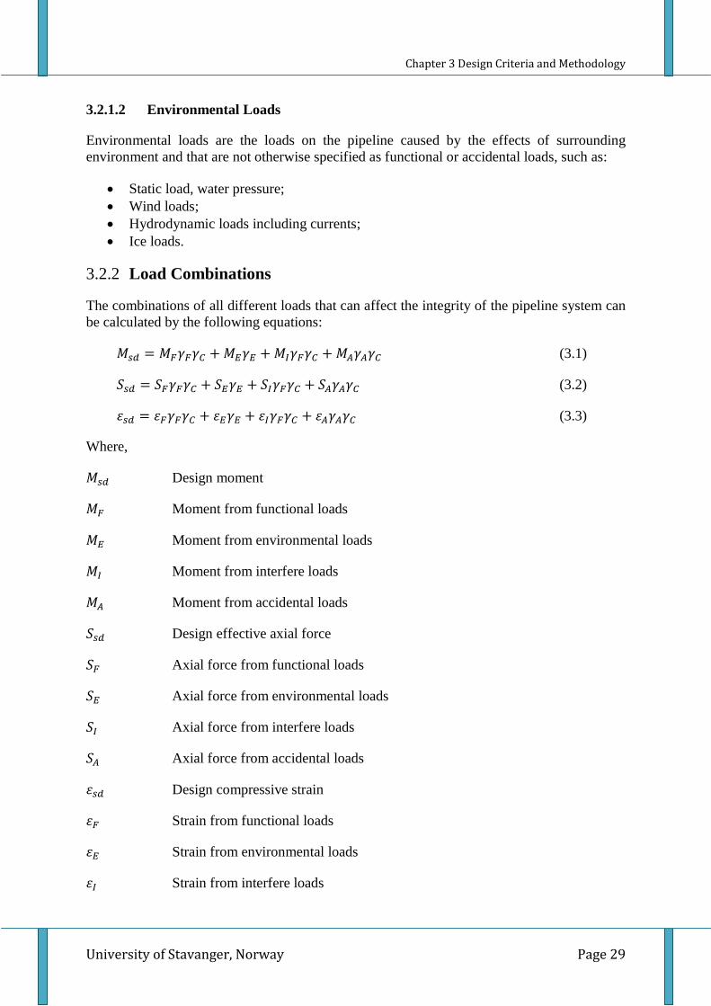
The combinations of all different loads that can affect the integrity of the pipeline system can be calculated by the following equations:

𝑀𝑠𝑑 = 𝑀𝐹𝛾𝐹𝛾𝐶 + 𝑀𝐸𝛾𝐸 + 𝑀𝐼𝛾𝐹𝛾𝐶 + 𝑀𝐴𝛾𝐴𝛾𝐶 (3.1)

𝑆𝑠𝑑 = 𝑆𝐹𝛾𝐹𝛾𝐶 + 𝑆𝐸𝛾𝐸 + 𝑆𝐼𝛾𝐹𝛾𝐶 + 𝑆𝐴𝛾𝐴𝛾𝐶 (3.2)

𝜀𝑠𝑑 = 𝜀𝐹𝛾𝐹𝛾𝐶 + 𝜀𝐸𝛾𝐸 + 𝜀𝐼𝛾𝐹𝛾𝐶 + 𝜀𝐴𝛾𝐴𝛾𝐶 (3.3)

Where,

𝑀𝑠𝑑 Design moment

𝑀𝐹 Moment from functional loads

𝑀𝐸 Moment from environmental loads

𝑀𝐼 Moment from interfere loads

𝑀𝐴 Moment from accidental loads

𝑆𝑠𝑑 Design effective axial force

𝑆𝐹 Axial force from functional loads

𝑆𝐸 Axial force from environmental loads

𝑆𝐼 Axial force from interfere loads

𝑆𝐴 Axial force from accidental loads

𝜀𝑠𝑑 Design compressive strain

𝜀𝐹 Strain from functional loads

𝜀𝐸 Strain from environmental loads

𝜀𝐼 Strain from interfere loads



𝜀𝐴 Strain from accidental loads

𝛾𝐹 Load effect factor for functional load

𝛾𝐶 Conditional load effect factor

𝛾𝐴 Load effect factor for accidental load

The load combinations should be checked for each different design limit states as per Table 3-1. The ULS design load combinations are different due to differencies in the local buckling limit states.

Table 3-1: Load Effect Factors and Load Combinations, Ref [13]

Limit State/Load

Combination Design Load Combination

Functional Loads 1)

Environmental Load

Interference Loads

Accidental Loads

𝜸𝑭 𝜸𝑬 𝜸𝑬 𝜸𝑨

ULS System Check 2) 1.2 0.7

Load Check 1.1 1.3 1.1

FLS 1.0 1.0 1.0

ALS 1.0 1.0 1.0 1.0

1) If the functional load effect reduces the combined load effects, 𝛾𝐹 shall be taken as 1/1.1

2) This load combination shall only be checked when system effects are present, i.e. when the major part of the pipeline is exposed to the same functional load. This will typically only apply to pipeline installation.

The condition load effect factors in Table 3-2 are applied to calculate load combinations as presented in equations (3.1) to (3.3).

Table 3-2: Condition Load Effect Factors, Ref [13]

Condition Load Effect Factor, 𝜸𝑪

Condition 𝜸𝑪

Pipeline Resting on Uneven Seabed 1.07

Continuously Stiff Supported 0.82

System Pressure Test 0.93

Otherwise 1.00

3.2.3 Material Resistance Factor

According to the Load and Resistance Factor Design (LFRD) method, the material resistance factor should be taken into account for safety reasons. The material resistance factor (𝛾𝑚) is categorized as per DNV-OS-F101 requirement as shown in Table 3-3.



Table 3-3: Material Resistance Factor, Ref [13]

Material Resistance Factor, 𝜸𝒎

Limit State Category SLS/ULS/ALS FLS

𝛾𝑚 1.15 1.00

3.2.4 Safety Class Definition

Pipeline installation can be classified as low safety class. The reason is because there are not many human activities during pipeline installations and usually pipeline installations have low risk of human injuries and low environment impacts. But if the installation is exposed to higher risk to the personnel and environmental damage, a higher safety class shall be implemented. The safety class resistance factor (𝛾𝑠𝑐) is presented in Table 3-4.

Table 3-4: Safety Class Definition, Ref [13]

Safety Class Resistance Factors. 𝜸𝑺𝑪

Safety Class Low Medium High

Pressure Containment 1.046 1.138 1.308

Other 1.04 1.14 1.26

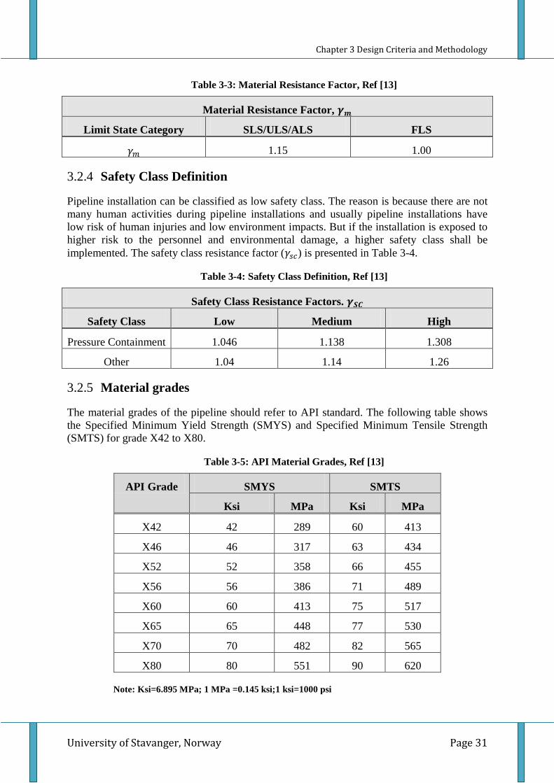
3.2.5 Material grades

The material grades of the pipeline should refer to API standard. The following table shows the Specified Minimum Yield Strength (SMYS) and Specified Minimum Tensile Strength (SMTS) for grade X42 to X80.

Table 3-5: API Material Grades, Ref [13]

API Grade SMYS SMTS

Ksi MPa Ksi MPa

X42 42 289 60 413

X46 46 317 63 434

X52 52 358 66 455

X56 56 386 71 489

X60 60 413 75 517

X65 65 448 77 530

X70 70 482 82 565

X80 80 551 90 620

Note: Ksi=6.895 MPa; 1 MPa =0.145 ksi;1 ksi=1000 psi



3.2.6 Characteristic material properties

Based on DNV 2007, the following equations for characteristic material strength 𝑓𝑦 and 𝑓𝑢 are used in the limit state criteria:

𝑓𝑦 = (𝑆𝑀𝑌𝑆 − 𝑓𝑦,𝑡𝑒𝑚𝑝)𝛼𝑢 (3.4)

𝑓𝑦 = (𝑆𝑀𝑌𝑆 − 𝑓𝑦,𝑡𝑒𝑚𝑝)𝛼𝑢 (3.5)

Where :

𝑓𝑦,𝑡𝑒𝑚𝑝; 𝑓𝑢,𝑡𝑒𝑚𝑝 ∶ are the de-rating value due to temperature, see Figure 3-1

𝛼𝑢 : Is the material strength factor, see Table 3-6

Table 3-6: API Material Strength Factor, 𝜶𝒖, Ref [13]

Material Strength Factor, 𝜶𝒖 Factor Normally Supplementary

Requirement 𝜶𝒖 𝛼𝑢 0.96 1.00

Based on the chart shown in Figure 3-1, C-Mn steel shall be considered for the temperature above 50o C and material 22 Cr and 25 Cr need to be considered for temperatures above 20o C.

Figure 3-1 : De-rating Values for Yield Stress of C-Mn and Duplex Stainless Steel, Ref [13]

3.2.7 Maximum fabrication factor

To accommodate the different strengths for pipes in tension and compression due to the manufacturing processes, a fabrication factor is normally used for pipeline design. The value of the maximum fabrication factor presented in Table 3-7 can be used in case there are no detailed informations available regarding the manufactoring process.



Table 3-7: Maximum Fabrication Factor, Ref [13]

Maximum Farication Factor, 𝜶𝒇𝒂𝒃

Pipe Seamless UO&TRB&ERW UOE

𝛼𝑓𝑎𝑏 0.96 0.93 0.85

3.3 Limit State A Limit State is the condition where the structure is not able to satisfy the requirements. Limit states for pipelines can be categorized as, Ref [13]:

• Serviceability Limit State (SLS): Pipeline must be able to continue its function when subjected to routine loads;

• Ultimate Limit State (ULS): A condition that if the criterion is exceeded, it can endanger the integrity of the pipeline system;

• Accidental Limit State (ALS): the pipeline shall be able to withstand accidental or unplanned loads such as dropped object, fire, impact from fishing trawl, and so on. ALS consition also known as ULS condition due to accident (in-frequent) loads;

• Fatigue Limit State (FLS): The pipeline needs to be designed to sustain accumulated cyclic dynamic loads during the operations.

Based on DNV-OS-F101, the design load (LSd) shall not exceed the resistance factor design (RRd). It can be expressed by following equation:

𝑓 �� 𝐿𝑠𝑑𝑅𝑅𝐷

�� ≤ 1 (3.6)

3.3.1 Ovalization

The condition that is characterized by changing the pipeline cross section from its original shape (circle) into an elliptic shape is known as ovalization. During the pipeline installation process, the pipe will be exposed to bending, either in the elastic or plastic regime. If it is occured in the plastic regime, the pipeline cross section will experience permanent deformations. This condition will reduce the pipe’s resistance to external pressure that can cause the collapse and pigging problem for the pipeline.

Mechanism of ovalization is shown in Figure 3-2. Figure 3-2 (a) shows the longitudinal stress phenomena due to combination of bending and external pressure. The lower part will experience tension while the upper part will experience compression. This condition will cause ovality of the pipe, see Figure 3-2 (b) for illustration.



Figure 3-2 : Ovalizationduring Bending,Ref [26]

𝑓0 = 𝐷𝑚𝑎𝑥−𝐷𝑚𝑖𝑛𝐷

(3.7)

Where:

f0 the out of roundness of the pipe, prior to loading (Initial ovality). Not to be taken < 0.005, Ref [13]

Dmax Greatest measured inside or outside diameter

Dmin Smallest measured inside or outside diameter

D Outer diameter of the pipe

Based on DNV-OS-F101 (2007), the out of roundness tolerance from fabrication together with flattening due to bending should not exceed 3%, except when there are some special considerations, such as if:

• A corresponding reduction in moment resistance has been included; • Geometrical restrictions are met, such as pigging requirements; • Additional cyclic stresses caused by the ovalization have been considered; • Tolerances in the relevant repair system are met.

Any point along the pipeline subjected to a point load, such as at freespan shoulders, artificial supports, and support settlements must be checked for ovalization.



3.4 Stability and Wall Thickness Design Criteria

3.4.1 On BottomStability

The pipeline should not move from its installed position even under extreme loading conditions. To satisfy this requirement, the pipeline must be supported, anchored in an open trench or be buried. These conditions do not include permissible lateral or vertical movements, thermal expansion, and a limited amount of settlement after installation.

For on-bottom stability purposes, the submerged weight of the pipeline should be higher than the buoyancy loads.

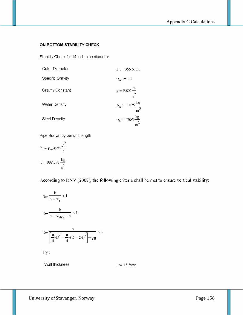
According to DNV (2007), the following criteria shall be met to ensure vertical stability:

𝛾𝑤𝑏

𝑤𝑠+𝑏≤ 1.0 (3.8)

Where:

𝑏 = 𝜌𝑤𝑔𝜋𝐷2

4 (3.9)

𝛾𝑤 Safety factor. Can be applied as 1.1 if a sufficiently low probability of negative buoyancy is not documented

ws Pipe submerged weight per unit length

b Pipe buoyancy per unit length

D Outer diameter of the pipe including all coatings

g Gravity acceleration; 9.81m/s2

𝜌𝑤 Mass density of water; 1025 kg/m3 for sea water

3.4.2 Local Buckling

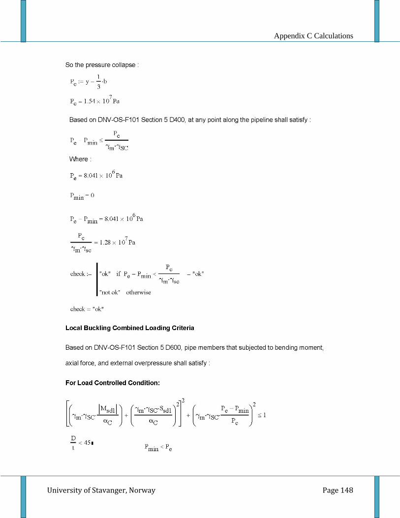
In deep water conditions, the pipeline may experience local buckling because there is high external hydrostatic pressure. Local buckling initially will occur in the weakest point of the pipeline and lead to pipe collapse failure. As a result, ovalization will occur and lead to buckling propagation especially in deep water conditions.

Based on DNV (2007) any locations along the pipeline should satisfy the following criteria:

𝑃𝑒 − 𝑃𝑚𝑖𝑛 ≤𝑃𝑐(𝑡1)𝛾𝑚𝛾𝑆𝐶

(3.10)

Where:



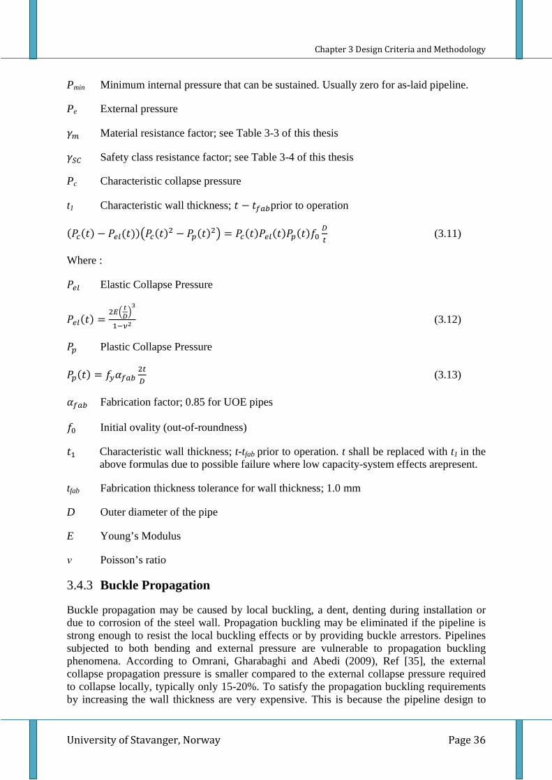
Pmin Minimum internal pressure that can be sustained. Usually zero for as-laid pipeline.

Pe External pressure

𝛾𝑚 Material resistance factor; see Table 3-3 of this thesis

𝛾𝑆𝐶 Safety class resistance factor; see Table 3-4 of this thesis

Pc Characteristic collapse pressure

t1 Characteristic wall thickness; 𝑡 − 𝑡𝑓𝑎𝑏prior to operation

(𝑃𝑐(𝑡) − 𝑃𝑒𝑙(𝑡))�𝑃𝑐(𝑡)2 − 𝑃𝑝(𝑡)2� = 𝑃𝑐(𝑡)𝑃𝑒𝑙(𝑡)𝑃𝑝(𝑡)𝑓0𝐷𝑡 (3.11)

Where :

𝑃𝑒𝑙 Elastic Collapse Pressure

𝑃𝑒𝑙(𝑡) =2𝐸�𝑡𝐷�

3

1−𝜈2 (3.12)

𝑃𝑝 Plastic Collapse Pressure

𝑃𝑝(𝑡) = 𝑓𝑦𝛼𝑓𝑎𝑏2𝑡𝐷

(3.13)

𝛼𝑓𝑎𝑏 Fabrication factor; 0.85 for UOE pipes

𝑓0 Initial ovality (out-of-roundness)

𝑡1 Characteristic wall thickness; t-tfab prior to operation. t shall be replaced with t1 in the above formulas due to possible failure where low capacity-system effects arepresent.

tfab Fabrication thickness tolerance for wall thickness; 1.0 mm


E Young’s Modulus

ν Poisson’s ratio

3.4.3 Buckle Propagation

Buckle propagation may be caused by local buckling, a dent, denting during installation or due to corrosion of the steel wall. Propagation buckling may be eliminated if the pipeline is strong enough to resist the local buckling effects or by providing buckle arrestors. Pipelines subjected to both bending and external pressure are vulnerable to propagation buckling phenomena. According to Omrani, Gharabaghi and Abedi (2009), Ref [35], the external collapse propagation pressure is smaller compared to the external collapse pressure required to collapse locally, typically only 15-20%. To satisfy the propagation buckling requirements by increasing the wall thickness are very expensive. This is because the pipeline design to



avoid propagation buckling is too conservative, therefore other solutions could become alternatives to avoid damagesby propagations. The probability of the occurence of propagating buckling in long distance can be decreased by installing buckle arrestors in the pipelines (Figure 3-3).

𝑃𝑒 < 𝑃𝑝𝑟𝛾𝑚𝛾𝑆𝐶

(3.14)

Where:

𝛾𝑚 Material resistance factor; see Table 3-3

𝛾𝑆𝐶 Safety class resistance factor; see Table 3-4

𝑃𝑒 External pressure

𝑃𝑝𝑟 Propagating pressure

𝑃𝑝𝑟 = 35𝑓𝑦𝛼𝑓𝑎𝑏 �𝑡2𝐷�2.5

, 𝐷𝑡2

< 45 (3.15)

𝑓𝑦 Characteristic yield stress

𝛼𝑓𝑎𝑏 Fabrication factor

𝑡2 Characteristic wall thickness; t for pipelines prior to installation


3.4.4 Buckle Arrestor

Bending stiffness increases by providing buckle arrestors. These buckle arrestors are placed at some intervals along the pipeline, then the pipeline damage due to collapse propagation can be reduced.



Figure 3-3 : Three Types of Buckle Arrestors,Ref [26]

According to DNV (2007), Ref [13], an integral buckle arrestor can be designed based on the following equation:

𝑃𝑒 ≤𝑃𝑥

1.1𝛾𝑚𝛾𝑆𝐶 (3.16)

Where:

𝛾𝑚 Material resistance factor; see Table 3-3 of this thesis

𝛾𝑆𝐶 Safety class resistance factor; see Table 3-4 of this thesis

𝑃𝑒 External pressure

𝑃𝑥 Crossover pressure

𝑃𝑥 = 𝑃𝑝𝑟 + �𝑃𝑝𝑟,𝐵𝐴 − 𝑃𝑝𝑟� �1 − 𝐸𝑋𝑃 �−20 𝑡2𝐿𝐵𝐴𝐷2

�� (3.17)

Where:

𝑃𝑝𝑟,𝐵𝐴 Propagating buckle capacity of an infinite arrestor

𝑃𝑝𝑟 Propagating pressure

𝐿𝐵𝐴 Buckle arrestor length

𝑡2 Characteristic wall thickness; t for pipelines prior to operation



The capacity of the buckle arrestor depends on, Ref [13]:

• The propagation buckle resistance from the adjacent pipe;

• Propagating buckle resistance of an infinite buckle arrestor;

• The arrestor length.

3.5 Laying Design Criteria The pipeline installation analysis should be performed based on DNV-OS-F101 (2007) for Submarine Pipeline System.

3.5.1 Simplified Laying Criteria

For preliminary design of local buckling, the simplified laying criteria can be used according to DNV-OS-F101 2007 section 13 H300. Limit states for concrete crushing, fatigue and rotation should be checked as additional requirements.

Overbend

Based on DNV-OS-F101-2007, for static loading the strain in the overbend region should not exceed the criterion I in Table 3-8. The strain should consider the effects of bending, axial loads, and local roller loads. Effects due to varying stiffness (e.g. strain concentration at field joints or buckle arrestors) do not need to be included. For static plus dynamic loading, the strain in the overbend region should not exceed the criterion II in Table 3-8. The strain should consider all effects, including varying stiffness due to field joints or buckle arrestors.

Table 3-8: Simplified Criteria for Overbend, Ref [13]

Simplified Criteria for Overbend

Criterion X70 X65 X60 X52

I 0.270 % 0.250 % 0.230 % 0.205 %

II 0.325 % 0.305 % 0.290 % 0.260 %

Sagbend

For combination of static and dynamic loads, the following equation shall be satisfied both in the sagbend and at the stinger tip:

𝜎𝑒𝑞 < 0.87𝑓𝑦 (3.18)

Where:

𝑓𝑦 = 𝑦𝑖𝑒𝑙𝑑 𝑠𝑡𝑟𝑒𝑠𝑠

𝜎𝑒𝑞 = 𝑒𝑞𝑢𝑖𝑣𝑎𝑙𝑒𝑛𝑡 𝑠𝑡𝑟𝑒𝑠𝑠



Effects due to varying stiffness or residual strain from the overbend can be ignored. For installation in deeper water, where collapse is a potential problem, the sagbend should meet the requirements for buckling criteria in DNV-OS-F101 Section 5 D600. The pipelines in the sagbend region should be designed based on load controlled condition criteria.

3.5.2 Local Buckling – Combined Loading Criteria

For pipeline installation in deepwater, local buckling is one of the criteria that has high potential to damage the pipeline system during lay operation. There are two conditions that need to be considered for checking local buckling of the pipeline:

• Load Controlled condition (LC condition);

• Displacement Controlled condition (DC condition).

3.5.2.1 Load Controlled Condition

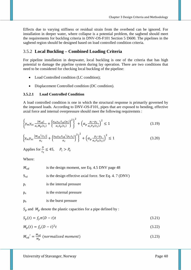
A load controlled condition is one in which the structural response is primarily governed by the imposed loads. According to DNV-OS-F101, pipes that are exposed to bending, effective axial force and internal overpressure should meet the following requiremnts :

�𝛾𝑚𝛾𝑠𝑐|𝑀𝑠𝑑|

𝛼𝑐𝑀𝑝(𝑡2) + �𝛾𝑚𝛾𝑠𝑐𝑆𝑠𝑑(𝑝𝑖)𝛼𝑐𝑆𝑝(𝑡2) �

2�2

+ �𝛼𝑝𝑝𝑖−𝑝2

𝛼𝑐𝑃𝑏(𝑡2)�2≤ 1 (3.19)

�𝛾𝑚𝛾𝑠𝑐�𝑀𝑠𝑑

′(𝑡2)�𝛼𝑐

+ �𝛾𝑚𝛾𝑠𝑐𝑆𝑠𝑑′(𝑝𝑖,𝑡2)

𝛼𝑐�2�2

+ �𝛼𝑝𝑝𝑖−𝑝2

𝛼𝑐𝑃𝑏(𝑡2)�2≤ 1 (3.20)

Applies for 𝐷𝑡2≤ 45, 𝑃𝑖 > 𝑃𝑒

Where:

𝑀𝑠𝑑 is the design moment, see Eq. 4.5 DNV page 48

Ssd is the design effective axial force. See Eq. 4. 7 (DNV)

pi is the internal pressure

pe is the external pressure

pb is the burst pressure

𝑆𝑝 and 𝑀𝑝 denote the plastic capacities for a pipe defined by :

𝑆𝑝(𝑡) = 𝑓𝑦𝜋(𝐷 − 𝑡)𝑡 (3.21)

𝑀𝑝(𝑡) = 𝑓𝑦(𝐷 − 𝑡)2𝑡 (3.22)

𝑀𝑠𝑑′ = 𝑀𝑠𝑑

𝑀𝑝 (𝑛𝑜𝑟𝑚𝑎𝑙𝑖𝑠𝑒𝑑 𝑚𝑜𝑚𝑒𝑛𝑡) (3.23)



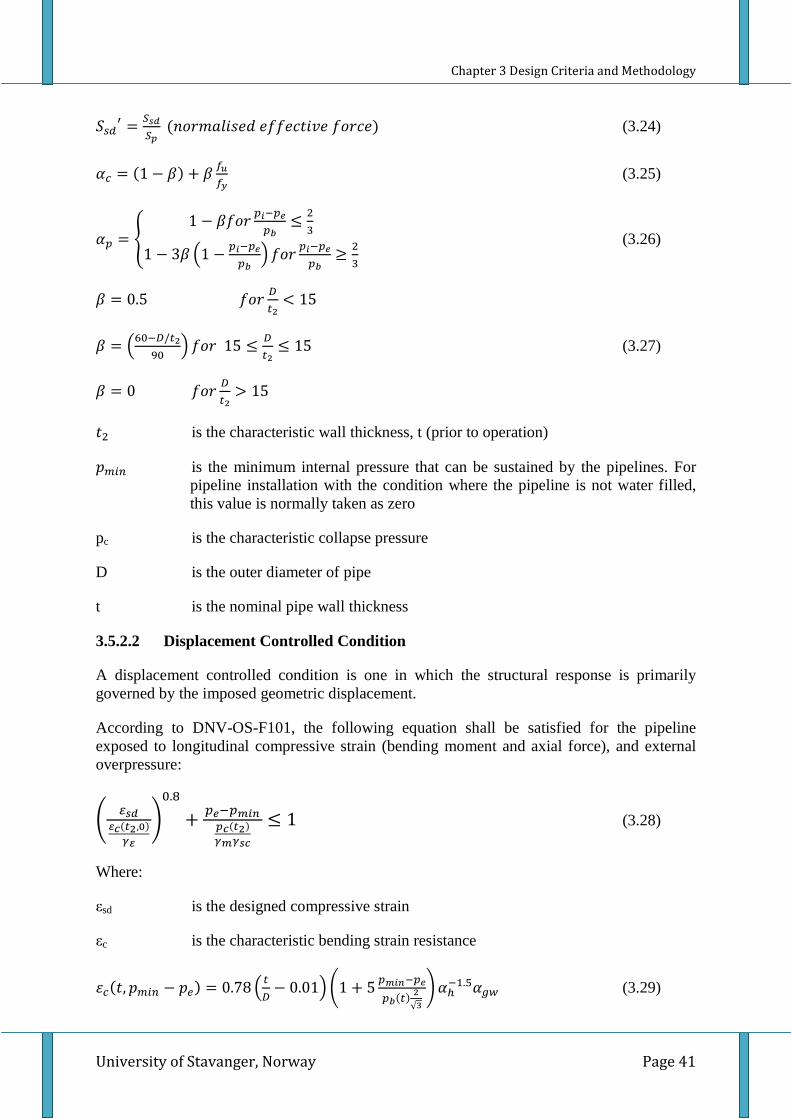
𝑆𝑠𝑑′ = 𝑆𝑠𝑑𝑆𝑝

(𝑛𝑜𝑟𝑚𝑎𝑙𝑖𝑠𝑒𝑑 𝑒𝑓𝑓𝑒𝑐𝑡𝑖𝑣𝑒 𝑓𝑜𝑟𝑐𝑒) (3.24)

𝛼𝑐 = (1 − 𝛽) + 𝛽 𝑓𝑢𝑓𝑦

(3.25)

𝛼𝑝 = �1 − 𝛽𝑓𝑜𝑟 𝑝𝑖−𝑝𝑒

𝑝𝑏≤ 2

3

1 − 3𝛽 �1 − 𝑝𝑖−𝑝𝑒𝑝𝑏

� 𝑓𝑜𝑟 𝑝𝑖−𝑝𝑒𝑝𝑏

≥ 23

(3.26)

𝛽 = 0.5 𝑓𝑜𝑟 𝐷𝑡2

< 15

𝛽 = �60−𝐷/𝑡290

� 𝑓𝑜𝑟 15 ≤ 𝐷𝑡2≤ 15 (3.27)

𝛽 = 0 𝑓𝑜𝑟 𝐷𝑡2

> 15

𝑡2 is the characteristic wall thickness, t (prior to operation)

𝑝𝑚𝑖𝑛 is the minimum internal pressure that can be sustained by the pipelines. For pipeline installation with the condition where the pipeline is not water filled, this value is normally taken as zero

pc is the characteristic collapse pressure

D is the outer diameter of pipe

t is the nominal pipe wall thickness

3.5.2.2 Displacement Controlled Condition

A displacement controlled condition is one in which the structural response is primarily governed by the imposed geometric displacement.

According to DNV-OS-F101, the following equation shall be satisfied for the pipeline exposed to longitudinal compressive strain (bending moment and axial force), and external overpressure:

� 𝜀𝑠𝑑𝜀𝑐(𝑡2,0)

𝛾𝜀

�0.8

+ 𝑝𝑒−𝑝𝑚𝑖𝑛𝑝𝑐(𝑡2)𝛾𝑚𝛾𝑠𝑐

≤ 1 (3.28)

Where:

εsd is the designed compressive strain

εc is the characteristic bending strain resistance

𝜀𝑐(𝑡,𝑝𝑚𝑖𝑛 − 𝑝𝑒) = 0.78 �𝑡𝐷− 0.01� �1 + 5 𝑝𝑚𝑖𝑛−𝑝𝑒

𝑝𝑏(𝑡) 2√3

�𝛼ℎ−1.5𝛼𝑔𝑤 (3.29)



D is the outer diameter of pipe

t is the nominal pipe wall thickness

αh is the minimum strain hardening, refer to DNV-OS-F101 (2007) section 7 Table 7-5 page71

𝛼ℎ = �𝑅𝑡0.5𝑅𝑚

�𝑚𝑎𝑥

(3.30)

αgw is the girth weld factor, refers to DNV-OS-F101 (2007) section 13 E1000.

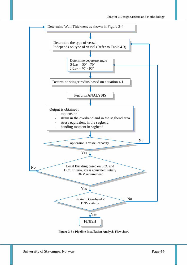
3.6 Design Methodology Iteration processes are required in pipeline installation to find out the optimum configuration in certain conditions. The design methodology is shown in Figure 3-4 and Figure 3-5.

Figure 3-4 presents the sequence of wall thickness design. Wall thickness should be designed to avoid :

• Bursting (pressure containment);

• Local buckling or collapse due to combination of external pressure and bending moment;

• Propagating buckling.

Once the required wall thickness has been choosen, the pipeline installation analysis can be done with sequence as presented in Figure 3-5. This sequence is repeated for different pipe diameters in various water depths.



Figure 3-4 : Wall Thickness Design Flowchart, Ref [20]

START

Define pressures for pressure containment

Criteria

Select wall thickness and

define minimum thickness

Increase Wall Thickness Yes

Yes No

Check pressure containment

Criteria

OK ?

Select pressure for hydrostatic

collapse

Check for hydrostatic

collapse

OK ?

Repeat for combined loading

Increase Wall Thickness

END

No



Figure 3-5 : Pipeline Installation Analysis Flowchart

Top tension < vessel capacity

Local Buckling based on LCC and DCC criteria, stress equivalent satisfy

DNV requirement

Strain in Overbend < DNV criteria

No

Yes

Yes

No

No

Yes

FINISH

Output is obtained : - top tension - strain in the overbend and in the sagbend area - stress equivalent in the sagbend - bending moment in sagbend

Perform ANALYSIS

Determine stinger radius based on equation 4.1

Determine departure angle S-Lay = 50o – 70o J-Lay = 70o - 90o

Determine the type of vessel. It depends on type of vessel (Refer to Table 4.3)

Determine Wall Thickness as shown in Figure 3-4

Chapter 4 Analysis Study


CHAPTER 4 ANALYSIS STUDY

This chapter presents the inputs, assumptions and modeling part for the static analysis performed by SIMLA. The purpose of this study is to evaluate the possibility of installing different diameter pipelines in various water depths.

Lay analyses were carried out using SIMLA software to get some results:

• Pipeline layability for various pipe diameters and water depths with S-Lay and J-lay method;

• Effects of increasing the allowable overbend strain criteria (up to 0.5%);

• Effects on the installation process by increasing the steel grade to X70, X80, and X100, respectively;

• Effects of reducing the length of stinger.

4.1 Pipelay Parameter The following parameters have significant effects on the pipe lay analysis, Ref [4] :

• Stinger radius (for S-lay);

• Roller position (for S-Lay);

• Departure angle;

• Pipelay tension;

• Pipe bending stiffness;

• Pipe weight;

• Water depth.

During pipeline installation, the above parameters will change some factors, such as :

• Top tension;

• Overbend strains (S-lay);

• Sagbend bending moments;

• Contact-force between pipe and seabed.

As explained in section 3, the following criteria can be used for preliminary design during installation analysis :



• Sagbend:

Combination of bending moment and external pressure in the sagbend region is checked using a Load Controlled condition (LCC) criteria based on DNV (2007). Refer to section 3.5.2 of this report.

• Overbend:

The overbend region is checked using a Displacement Controlled Condition (DCC) criteria and should satisfy the strain requirement as given in Table 3-8. For sensitivity study, a maximum allowable overbend strain criterion of 0.5% is used.

Material parameters presented in Table 4-1 are used in this study considering the following location and safety class, Ref [13]:

• Location class 1: there are not much human activities.

• Clasified as a low safety class because the pipeline installation operations have low risk of human injuries, low environmental impacts and minor economic consequences.

Table 4-1: Material Parameter

Factor Class Value

Material resistance factor, 𝛾𝑚 SLS/ULS/ALS 1.15 Safety class resistance factor, 𝛾𝑆𝐶 LOW 1.04

Material strength factor, 𝛼𝑈 NORMAL 0.96

Maximum fabrication factor, 𝛼𝑓𝑎𝑏 UOE 0.85

Temperature de-rating None

Condition load effect factor, 𝛾𝐶 Pipe resting on uneven seabed 1.07

Minimum Strain Hardening 0.93

4.2 Pipelay Study Input

4.2.1 Pipeline Data

The pipeline data used in this study are presented in Table 4-2.



Table 4-2: Material Properties

Characteristics Unit Values

Carbon Steel Pipe

Inch 14, 20, 28, and 30

Density kg/m3 7850

Young’s Modulus

MPa 2.00 x 105

Poisson’s Ratio - 0.3

Ovality 1.5%

4.2.2 Environmental Data

4.2.2.1 Water Depth

This study considers pipeline installations in water depths of 800 m, 1300 m, 2000 m, 2500 m, 3000 m, 3500 m and 4000 m.

4.2.2.2 Seawater Properties

Seawater density is 1025 kg/m3 and minimum temperature is assumed to be 5.0oC.

4.2.2.3 Seabed Friction

The seabed friction is assumed to be: 0.3 in x and y direction.

4.2.3 Lay Vessel Data

Table 4-3 and Table 4-4 present the vessels’ data for S-Lay and J-lay respectively.

Table 4-3: S-Lay Vessel Data

Lay Vessel Minimum

Stinger Radius (m)

Tension Capacity

Stinger Length Ramp Height Ramp Angle

Pieter Schelte 70 2000 t, Ref [1] 170 m - 0o

Solitaire 70 1050 t 140 m 10.5 m 0o

Castorone 70 750 t 120 m - -

Lorelay 70 135 t 118 m 12.0 m 0o

Allseas Company has awarded a contract to build the world’s largest pipelay vessel. This vessel, Pieter Schelte is a dynamic positioned (DP) vessel. With a dynamic positioned system, the vessel has better ability to operate in deeper water depth compared to anchored vessel. Pieter Schelte has topside lift capacity of 48000 t, jacket lift capacity of 25000 t and pipelay tension capacity around 2000 t, Ref [1]. This tension capacity will be doubling the



capacity of Allseas’ Solitaire. Pieter Schelte is supposed to be ready for offshore operation in early 2014.

Table 4-4: J-Lay Vessel Data

Lay Vessel Tension Capacity Lay Angle

Aegir (Herema) 2000 t, Ref [17]

Balder 1050 t 50-90

Saipem 7000 525 t 90-110

Deep Blue 770 t 58-90

Aegir is a new deepwater construction vessel (DCV) with capability to execute complex infrastructure and pipeline J-Lay installation in ultra-deep water, Ref [17].

4.2.4 Assumptions

Some assumptions are used in this study and outlined in the following list:

• Only static analyses will be carried out because the study is only a general study and performed for no specific location. In an actual project, a dynamic analysis should be performed especially in case of static analyses with critical result i.e. close to installation limits;

• The seabed is assumed to be flat, continuous and elastic. In reality the seabed may be uneven and probably it would have varied topography and different soil types and potentially rocks;

• The pipeline is assumed to be empty during installation;

• Pipeline coating is not considered during installation analysis. In actual conditions, coating thickness may be presented and the effect of this coating should be taken into consideration. The coating thickness will be different from one location to another, depending on location and water depth. The higher the thickness of the coating the bigger the pipeline weight will be. Furthermore the heavier pipelines require vessels with higher tension capability;

• For the S-Lay method, 3 types of vessel which are characterized by different stinger lengths are considered for each water depth (800-4000m). Furthermore the optimum configuration that satisfy the installation criteria will be chosen. Using the following equation, the departure angle can be estimated depending on the stinger length and stinger radius, Ref [23];

𝜉 = 30𝑅𝑠𝑡𝑖

. 1802𝜋

+ (𝐿𝑠𝑡𝑖−30)𝑅𝑠𝑡𝑖

180𝜋

+ 𝛼𝑟𝑎𝑚𝑝−𝑎𝑛𝑔𝑙𝑒 (4.1)

Where:

𝜉 : Departure Angle

𝑅𝑠𝑡𝑖 : Stinger Radius



𝐿𝑠𝑡𝑖 : Stinger Length

𝛼𝑟𝑎𝑚𝑝−𝑎𝑛𝑔𝑙𝑒 : Stinger/Ramp angle

The stinger radius can be adjusted depending on the water depth, but as far as possible the radius is set so that the top tension is still within the capacity of existing lay vessels. The relationship between departure angle and stinger radius for each vessel are presented in Figure 4-1 and Table 4-5.

Table 4-5: Stinger Radius vs Departure Angle

Stinger Radius (Rsti)

Departure Angle (degree)

Lorelay (Lsti =118 m)

Castorone (Lsti =120m)

Solitaire (Lsti =140 m)

Pieter Schelte (Lsti =170 m)

50 118.09 120.38 143.31 177.71

60 98.41 100.32 119.43 148.09

70 84.35 85.99 102.37 126.93

80 73.81 75.24 89.57 111.07

90 65.61 66.88 79.62 98.73

100 59.04 60.19 71.66 88.85

110 53.68 54.72 65.14 80.78

120 49.20 50.16 59.71 74.04

130 45.42 46.30 55.12 68.35

140 42.17 42.99 51.18 65.82

150 39.36 40.13 47.77 59.24

160 36.90 37.62 44.79 55.53

170 34.73 35.41 42.15 52.27

180 32.80 33.44 39.81 49.36



Figure 4-1 : Stinger Radius vs Departure Angle

Other parameters used in this study are given in the following list:

S-Lay

• Departure angle typically between 45o to 70o;

• Minimum stinger radius is 70 m;

• Maximum top tension is 2000t (Pieter Schelte);

• Minimum gap between the last roller and the pipe is 300mm (based on engineering judgment to allow dynamic effects);

• The strains in the overbend and the tension capacity of the lay vessel give the limitation for S-Lay installation.

J-Lay

• Departure angle typically between 70o to 90o;

• Maximum top tension is 2000t (Aegir Herema Vessel);

• Combination of bending moment and external pressure in the sagbend and the vessel’s tension capacity give limitations for J-lay method.

4.3 Pipelay Modeling Pipe lay analyses is carried out using SIMLA software. SIMLA is a finite element computer program for engineering analysis of offshore pipelines during design, installation and operations.

0102030405060708090

100110120130140150160170180190

0 50 100 150 200 250 300 350

Depa

rtur

e An

gle

(deg

)

Stinger Radius (m)

Departure Angle vs Stinger Radius

Pieter Schelte

Solitaire

Catastrone



As results of installation analysis, an optimum pipelay configuration and required tension are found. Specifically for S-Lay, the configuration of the stinger and the departure angle are known. Strain and stress in the overbend and sagbend region should satisfy the criteria mentioned in Section 3.5.

Some of the SIMLA features are:

• Non-linear static and dynamic Finite Element Analyses; • Global Buckling; • Bottom Roughness; • Pipelay; • Trawling/Anchor Hooking; • J-tube pull-in.

SIMLA also has some robust visualization tools such as :

• XPOST; • SIMVIS; • Routing and Intervention.

The important parameters of the pipelaying analyses such as strain in the overbend and sagbend, moment and axial tension along the pipe are provided by SIMLA as analyses output. The analysis is carried out so that the tension is kept within the existing vessel capacity by adjusting the stinger radius.

The global and local coordinate system in SIMLA is shown in Figure 4-2 and Figure 4-3, respectively. A right handed Cartesian coordinate system is applied, Ref [42]. In global axis, gravity is acting in the negative z-direction, where z positive is upwards and z negative is downward. Sea surface is situated at z = 0.

Figure 4-2 : Global Coordinate System in SIMLA, Ref [42]



Figure 4-3 : Local Coordinate System in SIMLA, Ref [42]

There are several modules in SIMLA. These modules are used at the sequence presented in the Figure 4-4.

Figure 4-4 : Purpose and Communication between Modules in SIMLA, Ref [42]

1. FlexEdit

FlexEdit is text editor used to present the input data that will be used in the analysis. The flexedit view is shown in Figure 4-5 and refers to Appendix A for the detailed input.

Flexedit SIMLA

XPost

SimVis

SIMPOST Matrix Plot

Generation of Input Files

Analysis Post Processing



Figure 4-5 : FlexEdit View 2. SIMLA

The purpose of this module is to run the analysis of the pipeline during design, installation and operation. Running analysis in SIMLA can be done using “Python” as shown in Figure 4-6 or using “Run button” in FlexEdit as shown in the Figure 4-5.

Figure 4-6 : Example of Run Operator in SIMLA using Python 3. XPOST

XPOST is 3D visualization program. The result of thenumerical model can be seen using XPOST. Figure 4-7 presents the example of lay analysis visualization.

Run button



Figure 4-7 : Example of XPOST View

4. SimVis

SimVis is part of the post processing module in SIMLA. This module presents 3D visualizations of the pipe and the surrounding environment such as the seabed feature in the 3D terrain model, Figure 4-8.

Figure 4-8 : Example of Simvis View



5. SIMPOST

Using SIMPOST module, the results generated by Simla can be extracted as detailed lists or plotted as a chart.

6. Matrix Plot

Matrix plot is one of SIMLA module that presents the plotting of the results extracted by SIMPOST. Anexample of a matrix plot view can be seen in Figure 4-9.

Figure 4-9 : Example of Result Visualization using Matrix Plot

4.3.1 S-Lay Model

The S-Lay model is shown in Figure 4-10.

Figure 4-10 : S-Lay Model

Seabed

Pipeline

Sea surface

X

Z



The sea is modeled as an arbitrary set of 4 noded shell elements. Each node is fixed for translation in x, y, and z directions. While pipe is modeled as a beam element structure.

Seabed/soil is modeled as spring support. Elastoplastic material is used for x and y directions while in z direction it is modeled as hyperelastic (nonlinear) material. SIMLA also provide facilities to model the route. Here one can also define how many lines will be used in the route. Each line defines the terrain of the seabed. The following figure presents example of route corridor with eleven lines.

Figure 4-11 : Example of a Route

The vessel is modeled as a rigid body. Constraint for vessel is specified as prescribe displacement type. In this case no displacement for translation in x, y, and z directions and also for rotation in x, y, z directions.

The connection between the pipe upper-end and the vessel is specified by a liniar constraint equation with factor of 1 for “master and slaves”. The concept of the “Master-Slave” facility is that the slave node will deflect as its master node.

Constraints at the pipe bottom end are specified as zero prescribing the displacement type for translations in x, y, and z directions.

The stinger geometry is represented by the roller configuration. The roller is modeled as a rigid body, fixed to the vessel for translation in z direction and for rotation in x and y directions. Figure 4-12 shows the roller position in this study.



Figure 4-12 : Roller Configurations

The pipe configuration for the S-lay method in SIMLA is specified by choosing the “S type” in the SIMLA card. With this command, the geometry is automaticaly formed depending on the water depth, pipe weight and departure angle. Deck height above the water is assumed to be 15 m.

4.3.1.1 Stinger Configuration

The roller position will be generated by SIMLA based on the stinger radius, stinger length and departure angle that are specified as input. Figure 4-13 shows the example of the roller configuration for 120 m stinger length. According to Table 4-3, the Castorone vessel has 120 m stinger length. Using the same stinger length, different departure angles can be adjusted based on water depth requirement.



Figure 4-13 : Roller Configurations with Various Departure Angle for 120 m Stinger Length

There are three different departure angles shown in Figure 4-13, i.e. 55 degree, 70 degree and 80 degree. The stinger radiuses are 110 m, 85 m, 80 m for 55 degree, 70 degree and 80 degree departure angles respectively. The relation between the departure angles, stinger radius and stinger length can be found inequation 4.1.

The roller configuration for 70 degree departure angle is steeper than the roller configuration for a 55 degree departure angle. Roller configuration with 80 degree departure angle is steeper than for 70 degree. The bigger departure angle, the steeper the roller configuration will be. Furthermore, the steeper configuration will create bigger strain in the overbend region but the required top tension will be decreased. This relation of strain in the overbend region and stinger configuration is studied in this thesis and presented in chapter 5.4.3.

4.3.2 J-Lay Model

The J-Lay model is shown in Figure 4-14.

-80

-70

-60

-50

-40

-30

-20

-10

0

10

-200 -150 -100 -50 0

Z Ax

is (m

)

X acxis (m)

Rolller Configurations with Various Departure Angle (Stinger Length = 120 m)

55-110-120

70-85-120

80-75-120



Figure 4-14 : J-Lay Model

As with the S-Lay model, the sea is modeled as an arbitrary set of 4 noded shell elements. Each node is fixed for translation in x, y, and z directions. While pipe is modeled as a beam element structure.

Seabed/soil modeled as spring support. Elastoplastic material is used for x and y directions while in the z direction the support is modeled as using hyperelastic (nonlinear) material.

The vessel is modeled as rigid body. Constraints for the vessel are specified as prescribing the displacement type. In this case no translation displacements in x, y, and z directions and also for rotation in x, y, z directions.

The connection between the pipe upper-end to the vessel is specified by a liniar constraint equation with factor of 1 for “master and slaves”. The concept of the “Master-Slave” facility is that the slave node will deflect as its master node.

Constraint at pipe bottom end is specified as zero prescribe displacement type for translation in x, y, and z directions.

Vessel Connection between pipe upper end and vessel

Sea

Flat Seabed

Pipeline

X

Y



The pipe configuration for the J-lay method in SIMLA is specified by choosing “J type” in SIMLA card. With this command, the geometry is automaticaly formed depending on the water depth, pipe weight and departure angle. Deck height above the water is assumed to be 15m.

Chapter 5 Results and Discussions


CHAPTER 5 RESULTS AND DISCUSSIONS

5.1 Wall Thickness Design The wall thickness is one of the most important parameters that need to be taken into consideration during the pipeline design phases. The wall thickness will determine the pipe’s capability to withstand internal and external pressure, the effect of corrosion, longitudinal stress as well as hoop stress. Furthermore, the wall thickness will influence the required tension during installation and the total cost of implementing the project.

Wall thickness should be designed to follow DNV specification to avoid, Ref [13]:

• Bursting (pressure containment);

• Local buckling (collapse);

• Propagating buckling.

High external hydrostatic pressure will cause high wall thickness requirement to avoid local buckling (collapse) and buckle propagation. However, using buckle propagation criteria to select wall thickness is not efficient and too expensive. Buckle arrestors are often provided to solve this problem.

The wall thickness requirement based on local buckling criterion (collapse) could be even bigger in deeper water. In the sagbend area, the pipe should be able to withstand local buckling due to combination of external pressure and bending moment based on Load Controlled Condition Criteria (LCC). While in the overbend area, the thickness should satisfy Displacement Controlled Criteria (DCC).

In deep and ultra deep waters the wall thicknesses are governed by external pressure and bending moment, therefore bursting (loss of pressure containment) is not considered in this thesis.

The minimum wall thicknesses for various water depths, various pipe diameters and various steel grades are shown in Table 5-1 to Table 5-3. The detailed calculation of wall thickness design based on local buckling and propagation buckling criteria are presented in APPENDIX C.



Local Buckling (System Collapse)

The minimum required wall thicknesses to satisfy local buckling criteria are presented in the following Table 5-1. The detailed concept and formula are described in chapter 3.

Table 5-1: Wall Thickness (mm) Based on Local Buckling (System Collapse)

Diameter Steel Grade

Water Depth (m) 800 1300 2000 2500 3000 3500 4000

14 inch

X65 11.8 14.8 17.8 20.3 23.8 27.0 30.0 X70 11.69 14.0 17.0 20.0 23.0 25.4 27.2 X80 11.52 13.8 16.8 18.8 21.0 23.0 25.0

X100 11.32 13.3 15.8 17.42 19.0 20.64 22.17

20 inch

X65 17.05 21.0 26.5 30.5 33.5 37.8 45.0 X70 16.85 20.5 25.4 29.0 33.0 36.2 41.0 X80 16.64 20.0 24.2 27.5 30.5 33.5 37.0

X100 16.34 19.3 23.0 25.35 27.49 29.8 32.4

28 inch

X65 23.94 30.0 37.5 43.0 48.0 54.0 60.0 X70 23.64 28.8 36.0 41.5 46.5 52.0 57.2 X80 23.3 28.0 34.2 39.0 43.0 47.5 52.2

X100 22.95 27.12 32.67 35.80 39.1 42.3 45.72

30 inch

X65 25.76 32.0 40.0 45.0 51.8 58.0 65.0 X70 25.51 31.0 38.6 44.3 50.0 56.0 61.5 X80 25.14 30.0 37.0 41.5 46.2 51.0 56.0

X100 24.68 29.0 35.0 38.6 42.03 45.36 49.0

Stability

For on bottom stability purposes, the submerged weight of the pipeline should be higher than the buoyancy weight. Considering 1.1 specific gravity for design stability, the wall thicknesses are obtained as shown in Table 5-2.

Table 5-2: Wall Thickness Based on Stability Criteria

Diamter Minimum Wall Thickness (mm) 14 inch 13.3 20 inch 19.1 28 inch 26.6 30 inch 28.5



Propagation Buckling

The minimum required wall thicknesses to satisfy propagation buckling criteria are presented in the following Table 5-3. The detailed concept and formula are described in chapter 3.

Table 5-3: Wall Thickness (mm) Based on Buckle Propagation


Water Depth (m) 800 1300 2000 2500 3000 3500 4000

14 inch

X65 21.0 25.3 29.9 32.6 35.0 37.1 39.1 X70 20.4 24.6 29.0 31.7 34.0 36.1 38.0 X80 19.4 23.4 27.6 31.7 32.3 34.3 36.1

X100 17.8 21.5 25.3 27.6 29.6 31.4 33.1

20 inch

X65 29.6 35.7 42.3 46.1 49.5 52.6 55.4 X70 28.8 34.7 41.1 44.8 48.1 51.1 53.9 X80 27.3 33.0 39.0 44.8 45.7 48.5 51.1

X100 25.1 30.2 35.7 39.0 41.8 44.4 46.8

28 inch

X65 41.0 49.6 58.8 64.2 68.9 73.3 77.2 X70 39.9 48.2 57.1 62.3 67.0 71.2 75.0 X80 37.9 45.8 54.2 62.3 63.5 67.5 71.2

X100 34.7 41.9 49.6 54.1 58.2 61.8 65.1

30 inch

X65 43.9 53.1 62.9 68.7 73.8 78.4 82.7 X70 42.7 51.6 61.1 66.7 71.7 76.2 80.3 X80 40.5 49.0 58.0 66.7 68.0 72.3 76.2

X100 37.1 44.8 53.1 57.9 62.3 66.2 69.7

The required wall thicknesses based on propagation buckling are very high compared to the required thicknesses based on local buckling criteria. Therefore it will not be considered in this study. In industry practice buckle arrestors are most often used to avoid buckle propagation.



5.1.1 Wall Thickness Summary

Considering the design parameters as explained above, the wall thicknesses that will be used in the analysis are summarized in the following Table 5-4.

Table 5-4: Wall Thickness Summary (mm)


Water Depth (m) 800 1300 2000 2500 3000 3500 4000

14 inch

X65 13.3 14.8 17.8 20.3 23.8 27.0 30.0 X70 13.3 14.0 17.0 20.0 23.0 25.4 27.2 X80 13.3 13.8 16.8 18.8 21.0 23.0 25.0

X100 13.3 13.3 15.8 17.42 19.0 20.64 22.17

20 inch

X65 19.1 21.0 26.5 30.5 33.5 37.8 45.0 X70 19.1 20.5 25.4 29.0 33.0 36.2 41.0 X80 19.1 20.0 24.2 27.5 30.5 33.5 37.0

X100 19.1 19.3 23.0 25.35 27.49 29.8 32.4

28 inch

X65 26.6 30.0 37.5 43.0 48.0 54.0 60.0 X70 26.6 28.8 36.0 41.5 46.5 52.0 57.2 X80 26.6 28.0 34.2 39.0 43.0 47.5 52.2

X100 26.6 27.12 32.67 35.80 39.1 42.3 45.72

30 inch

X65 28.5 32.0 40.0 45.0 51.8 58.0 65.0 X70 28.5 31.0 38.6 44.3 50.0 56.0 61.5 X80 28.5 30.0 37.0 41.5 46.2 51.0 56.0

X100 28.5 29.0 35.0 38.6 42.03 45.36 49.0

The graphical information of wall thickness requirement for 14 inch pipe diameter X65 based on various criteria is shown in Figure 5-1.



Figure 5-1 : Wall Thickness for Various for Various Limit States (X65)

5.1.2 Effect of Changing the Steel Grades

The effect of changing steel grades on the requirement of wall thickness has been shown in the previous section. This section presents the percent decrease in the required wall thickness for different steel grades.

Due to increasing the material grade from X65 to X100, in 800 meter water depth, the required wall thickness is decreased by:

• 0.48 mm or 4.1% for a 14 inch pipeline;



• 1.08 mm or 4.19 % for a 30 inch pipeline.

In 1300 meter water depth the required wall thickness is decreased by:




• 3.0 mm or 9.38% for a 30 inch pipeline.


-4500

-4000

-3500

-3000

-2500

-2000

-1500

-1000

-500

00 5 10 15 20 25 30 35 40 45

Wat

er D

epth

(m)

Wall Thickness (mm)

Wall Thickness vs Water Depth for Various Limit States (14" X65)

Specific grvt 1.1

Buckle Propagation

Local Buckling



• 2 mm or 11.24% for a 14 inch pipeline;



• 5 mm or 12.5% for a 30 inch pipeline.


















• 12.6 mm or 28% for a 20 inch pipeline;


• 16 mm or 24.62% for a 30 inch pipeline.

The results mentioned above shows that the effect of increasing the grade of steel is higher in 1300 m water depth compared to 800 m water depth. This effect is higher as increasing the water depth.



The graphical information about required wall thicknesses for various diameters in different water depths are presented in Figure 5-2 to Figure 5-5.

Figure 5-2 : D/t as Function of Steel Grades (14 Inch Diameter)


0,0

5,0

10,0

15,0

20,0

25,0

30,0

35,0

0 1000 2000 3000 4000 5000

D/t

Water Depth (m)

Water Depth vs D/t (14 inch Dia.)

X65

X70

X80

X100

0

5

10

15

20

25

30

35

0 1000 2000 3000 4000 5000

D/t

Water Depth (m)

D/t as function of Water Depth (20")

X65

X70

X80

X100




Figure 5-5 D/t as Function of Steel Grades (30 Inch Diameter)

5.1.3 Effects of Changing in Pipe Ovality

Pipe ovality also influences the wall thickness requierements. According to requirements of DNV OS F101 2007, bending and out of fabrication tolerances should not lead to flattening of more than 3%, except for special cases. In this thesis an ovality of 1.5% is used for all diameters and for all water depths.

Combination of hydrostatic external pressure and bending moment during installation tends to cause high pipe ovalities. The wall thickness should be strong enough to withstand the collapse or local buckling in deep and ultra deep water conditions. The required external pressure to buckle the pipe, known as collapse pressure (equation 3-11) will depend on the ratio of diameter to the thickness (D/t). Lower D/t ratio will allow higher external pressure before collapse, Ref [26].

0

5

10

15

20

25

30

35

0 1000 2000 3000 4000 5000

D/t

Water Depth (m)


X65

X70

X80

X100

05

101520253035

0 1000 2000 3000 4000 5000

D/t

Water Depth (m)


X65

X70

X80

X100



One of the objectives of this study is to carry out wall thickness design due to changes of pipe ovality from 0.5 % up to 3 %, which are the minimum and maximum values recommended by DNV OS F101 2007. The minimum wall thickness required for various pipe diameters and various water depths are provided in Table 5-5 to Table 5-8 and Figure 5-6 to Figure 5-9.

The results show that the wall thickness is decreased from 12 % up to 16 % due to the effect of reducing the ovality from 3% to 0.5%.

Table 5-5: 14 Inch X65 Wall Thickness (mm) vs Ovality

Water Depth (m)

Ovality (%) 0.5 1 1.5 2 2.5 3

800 10.80 11.10 11.75 12.09 12.42 12.73 1300 13.43 13.84 14.53 14.94 15.34 15.73 2000 17.12 17.66 18.41 18.93 19.44 19.92 2500 19.76 20.40 21.19 21.79 22.36 22.91 3000 22.39 23.14 23.96 24.64 25.28 25.90 3500 25.02 25.87 26.74 27.49 28.21 28.90 4000 27.66 28.61 29.51 30.34 31.13 31.89

For 14 inch pipe diameter, as the ovality decreases from 3% to 0.5% the required wall thickness is decreased by:

• 1.93 mm or 15.19 % in 800 m water depth • 2.29 mm or 14.58 % in 1300 m water depth • 2.28 mm or 14.04 % in 2000 m water depth • 3.16 mm or 13.77 % in 2500 m water depth • 3.51 mm or 13.57 % in 3000 m water depth • 3.87 mm or 13.40 % in 3500 m water depth • 4.23 mm or 13.27 % in 4000 m water depth


Water Depth (m)

Ovality (%) 0.5 1 1.5 2 2.5 3

800 15.84 16.37 16.87 17.35 17.82 18.28 1300 19.56 20.22 20.79 21.44 22.01 22.56 2000 24.78 25.62 26.29 27.16 27.87 28.56 2500 28.50 29.48 30.21 31.24 32.06 32.85 3000 32.22 33.34 34.14 35.33 36.25 37.13 3500 35.95 37.20 38.07 39.41 40.44 41.42 4000 39.67 41.05 41.99 43.50 44.62 45.70


• 2.44 mm or 13.35 % in 800 m water depth • 3.00 mm or 13.30 % in 1300 m water depth



• 3.79 mm or 13.26 % in 2000 m water depth • 4.35 mm or 13.23 % in 2500 m water depth • 4.91 mm or 13.22 % in 3000 m water depth • 5.47 mm or 13.20 % in 3500 m water depth • 6.03 mm or 13.19 % in 4000 m water depth


Water Depth (m)

Ovality (%) 0.5 1 1.5 2 2.5 3

800 22.17 22.91 23.61 24.29 24.95 25.59 1300 27.39 28.31 29.18 30.01 30.81 31.59 2000 34.68 35.87 36.97 38.02 39.02 39.99 2500 39.90 41.27 42.54 43.74 44.88 45.98 3000 45.11 46.68 48.11 49.46 50.75 51.98 3500 50.33 52.08 53.67 55.18 56.61 57.98 4000 55.54 57.48 59.24 60.90 62.47 63.98


• 3.42 mm or 13.35 % in 800 m water depth • 4.20 mm or 13.30 % in 1300 m water depth • 5.30 mm or 13.26 % in 2000 m water depth • 6.09 mm or 13.24 % in 2500 m water depth • 6.87 mm or 13.22 % in 3000 m water depth • 7.66 mm or 13.20 % in 3500 m water depth • 8.44 mm or 13.19 % in 4000 m water depth


Water Depth (m)

Ovality (%) 0.5 1 1.5 2 2.5 3

800 24.22 25.02 25.80 26.53 27.24 27.93 1300 29.84 30.83 31.78 32.67 33.53 34.36 2000 37.71 38.97 40.15 41.27 42.34 43.37 2500 43.33 44.78 46.13 47.41 48.63 49.81 3000 48.95 50.59 52.11 53.55 54.92 56.24 3500 54.57 56.39 58.09 59.69 61.21 62.68 4000 60.19 62.20 64.07 65.83 67.51 69.11


• 3.71 mm or 13.27 % in 800 m water depth • 4.52 mm or 13.15 % in 1300 m water depth • 5.66 mm or 13.05 % in 2000 m water depth • 6.47 mm or 12.99 % in 2500 m water depth • 7.29 mm or 12.95 % in 3000 m water depth



• 8.10 mm or 12.93 % in 3500 m water depth • 8.92 mm or 12.90 % in 4000 m water depth

Figure 5-6 : 14 Inch X65 Wall Thickness (mm) vs Ovality


0,00

5,00

10,00

15,00

20,00

25,00

30,00

35,00

0 1000 2000 3000 4000 5000

Wal

l Thi

ckne

ss (m

m)

Water Depth (m)

Water Depth vs Wall Thickness (14" X65)

Ovality 0.5%

Ovality 1%

Ovality 1.5%

Ovality 2%

Ovality 2.5%

Ovality 3%

0,00

5,00

10,00

15,00

20,00

25,00

30,00

35,00

40,00

45,00

50,00

0 1000 2000 3000 4000 5000

Wal

l Thi

ckne

ss (m

m)

Water Depth (m)


Ovality 0.5%

Ovality 1%

Ovality 1.5%

Ovality 2%

Ovality 2.5%

Ovality 3%





0,00

10,00

20,00

30,00

40,00

50,00

60,00

70,00

0 1000 2000 3000 4000 5000

Wal

l Thi

ckne

ss (m

m)

Water Depth (m)


Ovality 0.5%

Ovality 1%

Ovality 1.5%

Ovality 2%

Ovality 2.5%

Ovality 3%

0,00

10,00

20,00

30,00

40,00

50,00

60,00

70,00

80,00

0 1000 2000 3000 4000 5000

Wal

l Thi

ckne

ss (m

m)

Water Depth (m)


Ovality 0.5%

Ovality 1%

Ovality 1.5%

Ovality 2%

Ovality 2.5%

Ovality 3%



5.1.4 Discussion of Wall Thickness Parameter Study

The conclusions of the wall thickness parameter study are discussed below:

• Using higher steel grades will decrease the required wall thickness. This effect is getting higher as installation go to the deeper water. This is because the total pipe length extending from the vessel to the seabed is increased in deeper waters; therefore the submerged weight due to reduction of the thickness is decreased proportionally.

• Τhe reduction of wall thickness requirement due to increasing of steel grades is not depending significantly on the pipe diameter. The percentage of wall thickness reductions for 14 inch, 20 inch, 28 inch and 30 inch are close for the same water depth.

• The wall thickness is decreased by around 12 % and up to 16 % due to the effect of reducing the ovality from 3% to 0.5%. Therefore, ovality has significant influences on the wall thickness requirement.

• The effect of reducing the ovality from 3% to 0.5% is higher for bigger pipe diameter.

• The percentage of reduction is slightly smaller in deeper water for the same pipe diameter..

5.2 Required Top Tension

5.2.1 S-Lay Method

The analysis of pipelaying is carried out using the computer program SIMLA. As results the layability of the pipeline will be obtained. The results for X65 steel grade is summarized in the following Figure 5-10. The detailed results are presented in APPENDIX C.

The increasing of required top tension is linear up to 1300 m water depth. The reason is because the specific gravity requirement set the minimum value with small variations in wall thickness at water depth less than 1300 m. The wall thickness is increasing rapidly at water depth more than 1300 m to meet local buckling requirement. The impact is heavier pipes that needs vessel with bigger lay tension capacity. Beyond 2000 m the required top tension increase even steeper since the wall thickness increase rapidly due to higher external pressure in deep water condition.



Figure 5-10 : Required Top Tension as Function of Water Depth for S-Lay X65

Based on information from Figure 5-10 the following conclusions are obtained:

• The required top tensions for 14 inch pipe diameter are within the tension capacity of the existing lay vessel for all water depths. Castorone can be used for installation at water depth less than 3200m, while for 3200 m to 3700 m water depth, Solitaire can be used as a solution.

• The required top tension for 20 inch pipe diameter is higher compared to the requirement for 14 inch diameter. However it is still within the capacity of the most powerful upcoming S-Lay vessel, Pieter Schelte.

• For 28 inch pipe diameter, the required top tensions increase even steeper. Pieter Schelte can only possibly be used for installations in water depth less than 2900 m.

• And for 30 inch pipe diameter, Pieter Schelte can only possibly be used for installations in water depth less than 2650 m.

5.2.2 J-Lay Method

As with the S-Lay method, analysis by J-Lay is also carried out in this study, and the summary of the results are given in the Figure 5-11.

0

2000

4000

6000

8000

10000

12000

14000

16000

18000

20000

22000

24000

26000

28000

30000

32000

34000

36000

38000

40000

42000

44000

46000

48000

50000

52000

54000

56000

58000

60000

62000

64000

0 500 1000 1500 2000 2500 3000 3500 4000 4500

Requ

ired

Top

Tens

ion

(kN

)

Water Depth (m)

Water Depth vs Required Top Tension (S-Lay X65)

14 inch

20 inch

28 inch

30 inch

Castorone

Solitaire

Pieter Schelte



The increasing of required top tension is linear up to 1300 m water depth. The reason is because the specific gravity requirement set the minimum value with small variations in wall thickness at water depth less than 1300 m. The wall thickness is increasing rapidly at water depth more than 1300 m to meet local buckling requirement. The impact is heavier pipes that needs vessel with bigger lay tension capacity. Beyond 2000 m the required top tension increase even steeper since the wall thickness increase rapidly due to higher external pressure in deep water condition.

Figure 5-11 : Required Top Tension as Function of Water Depth for J-Lay X65

Based on information from Figure 5-11, the following conclusions are obtained:

• The required top tensions for 14 inch pipe diameter are within the tension capacity of existing lay vessel for all water depths. Saipem 7000 is possible to be used for installation at water depth less than 3550 m. For water depth more than 3550 m Deep Blue can be used as a solution

• The required top tension for 20 inch pipe diameter is higher compared to requirement for 14 inch diameter. However it is still within the capacity of the most powerful upcoming J-Lay vessels, Aegir (Herema).

• For 28 inch pipe diameter, the required top tension increases even steeper. Aegir (Herema) can only possibly be used for installation in water depth less than 3550m.

• And for 30 inch pipe diameter, Aegir (Herema) can only possibly be used for installation in water depth less than 3400 m.

0

2000

4000

6000

8000

10000

12000

14000

16000

18000

20000

22000

24000

26000

28000

30000

0 500 1000 1500 2000 2500 3000 3500 4000 4500

Requ

ired

Top

Tens

ion

(kN

)

Water Depth (m)

Water Depth vs Required Top Tension (J-Lay X65)

14 inch

20 inch

28 inch

30 inch

Saipem7000

Deep Blue

Balder

Aeigir (Herema)



5.3 Comparisons of S-Lay and J-Lay

5.3.1 14 inch Pipe Diameter

Figure 5-12 shows the comparison result of installation using S-Lay and J-Lay method for 14 inch pipe diameter.

Figure 5-12 : S-Lay and J-Lay Required Top Tension as Function of Water Depth (14”X65)

Based on information provided in Table 5-9 and Table 5-10, all the utilization factors are less than one; this means that the LCC (Load Control Condition) and the DCC (Displacement Control Condition) criteria are satisfied at all water depths for both S-lay and J-lay methods. DCC is a criterion that needs to be satisfied for the pipeline exposed .to longitudinal strain and external pressure. DCC criterion is used to check the overbend region. While LCC is a criterion that needs to be satisfied for the pipeline exposed .to bending, axial force and internal overpressure. LCC criterion is used to check the sagbend region.

Table 5-9: 14” Pipe S-Lay Result (X65)

Water Depth

(m)

Departure Angle

(deg)

Stinger Radius/Stinge

r Length

Wall Thickness

(mm) D/t

Top Tension

(kN)

Strain in Overbend

(%)

DCC Check

LCC Check

800 55 "110/120" 13.30 26.74 205.6 0.172 0.75 0.40 1300 55 "110/120" 14.80 24.03 692 0.198 0.92 0.65 2000 55 "110/120" 17.80 19.98 2171.42 0.235 0.99 0.78 2500 55 "110/120" 20.30 17.52 3890.18 0.268 0.99 0.83 3000 55 "110/120" 23.80 14.94 6029.89 0.303 0.96 0.85 3500 55 "130/140" 27.00 13.17 9515.38 0.31 0.96 0.99 4000 55 "130/140" 30.00 11.85 12025.1 0.38 0.97 0.91

Note: 1) Strain criteria is set as 0.25% 2) The detailed LCC and DCC calculations are presented in Appendix C

02000400060008000

100001200014000

0 1000 2000 3000 4000 5000

Requ

ired

Top

Tens

ion

(kN

)

Water Depth (m)

S-Lay & J-Lay Required Top Tension (14" X65)

S-Lay

J-Lay



The concusions of S-lay installation analysis for 14 inch diameter are:

• Required top tensions were found to be within the tension capacities of existing vessels at all water depths. Refer to Table 4-3 for the information about S-lay vessel capacity;

• Strain in overbend region is within the criteria of 0.25% for X65 at 800 m, 1300 m, and 2000 m water depth. Starting from 2500 m water depth, the strain criteria has been exceeded;

• Combinations of bending moment and external pressure in sagbend area (LCC Check) were less than one at all water depths;

• The pipe can be possibly installed with 55 ̊ departure angles for all water depth; • The distance between the last stinger roller and the pipe is set to be 300 mm for all cases.

Table 5-10: 14” Pipe J-Lay Result (X65)

Water Depth

(m)

Departure Angle

(deg)

Wall Thickness

(mm) D/t

Top Tension

(kN)

Strain in Sagben

d (%)

Stress Equivalent in

Sagbend (Mpa)

Allowable Stress (Mpa)

Sress Utilizati

on

LCC Check

800 86 13.30 26.74 122.41 0.096 210.00 389.76 0.54 0.40 1300 86 14.80 24.03 294 0.0850 170.00 389.76 0.44 0.66 2000 86 17.50 20.32 988.78 0.0700 140.00 389.76 0.36 0.78 2500 86 20.30 17.52 1819.7 0.0530 106.00 389.76 0.27 0.81 3000 86 22.80 15.60 3045.32 0.0720 144.00 389.76 0.37 0.76 3500 78 25.40 14.00 5021.16 0.0950 190.00 389.76 0.49 0.88 4000 78 28.60 12.43 6567.64 0.1160 232.00 389.76 0.60 0.87

The concusions of J-lay installation analysis for 14 inch diameter are:

• The required top tensions were found to be within the tension capacities of existing vessels at all water depths. Refer to Table 4-4 for the information about J-lay vessel capacity;

• Combinations of bending moment and external pressure in sagbend area (LCC Check) were less than one at all water depths;

• Stress equivalent in sagbend are inside the allowable stress at all water depths; • Departure angles are between 75 ̊- 90 ̊.


Figure 5-13 shows the comparison of the result of installation using S-Lay and J-Lay method for 20 inch pipe, see also Table 5-11 and Table 5-12.





Water Depth

(m)

Departure Angle (deg)

Stinger Radius/Stinger

Length

Wall Thickness

(mm) D/t

Top Tension

(kN)

Strain in Overbend

DCC Check

LCC Check

800 45 "134/120" 19.10 26.60 630 0.189 0.74 0.39 1300 45 "134/120" 21.00 24.19 1975.97 0.224 0.95 0.39 2000 58 "103/120" 26.50 19.17 4527.65 0.303 0.95 0.90 2500 60 "100/120" 30.50 16.66 7523.41 0.347 0.95 0.74 3000 60 "100/140" 33.50 15.16 10664.1 0.368 0.99 0.70 3500 65 "110/140" 37.80 13.44 13825.7 0.357 0.98 0.83 4000 65 "136/170" 45.00 11.29 21031 0.402 0.90 0.80


• Required top tensions were found to be within the tension capacities of existing vessel up to 2900 m water depth. However it is possible to perform pipeline installation up to 3900 m using the most powerfull upcoming S-Lay vessel (Pieter Schelte);

• Strain in overbend region is within the criteria of 0.25% for X65 only at 800 m and 1300 m water depth. Starting from 2000 m water depth, the strain criteria has been exceeded;

• Combinations of bending moment and external pressure in sagbend area (LCC Check) are less that one at all water depths;

• Departure angles are between 45 ̊- 70 ̊.

0

5000

10000

15000

20000

25000

0 1000 2000 3000 4000 5000Requ

ired

Top

Tens

ion

(kN

)

Water Depth (m


S-Lay

J-Lay



Table 5-12: 20” Pipe J-Lay Result (X65)

Water Depth

(m)


Wall Thickness

(mm) D/t

Top Tension

(kN)

Strain in Sagbend

(%)

Stress Equivalent in

Sagbend (Mpa)


Sress Utilizatio

n

LCC Check

800 86 19.10 18.62 258.86 0.125 250.0 389.76 0.64 0.39 1300 86 21.00 16.93 692.281 0.105 210.0 389.76 0.54 0.68 2000 86 24.40 14.57 1871 0.070 140.0 389.76 0.36 0.90 2500 86 28.00 12.70 3411.73 0.060 120.0 389.76 0.31 0.90 3000 86 34.50 10.31 6390.02 0.072 144.0 389.76 0.37 0.82 3500 78 37.80 9.41 10309.3 0.096 192.0 389.76 0.49 0.79 4000 75 45.00 7.90 11115.3 0.107 214.0 389.76 0.55 0.68


• Required top tensions were found to be within the tension capacities of existing vessels up to 3500 m water depths. However ; it is possible to perform pipeline installation up to 4000 m using the most powerfull upcoming J-Lay vessel (Aegir-Herema);

• Combinations of bending moment and external pressure in sagbend area (LCC Check) were less that one at all water depths;

• Stress equivalents in sagbend are inside the allowable stress at all water depths; • Departure angles are between 75 ̊- 90 ̊.


Figure 5-14 shows the comparison result of installation using S-Lay and J-Lay method for 28 inch pipe diameter, see also Table 5-13 and Table 5-14.


0

5000

10000

15000

20000

25000

30000

35000

40000

45000

0 1000 2000 3000 4000 5000

Requ

ired

Top

Tens

ion

(kN

)

Water Depth (m


S-Lay

J-Lay




Water Depth

(m)



Length

Wall Thickness

(mm) D/t

Top Tension

(kN)

Strain in Overbend

(%)

DCC Check

LCC Check

800 41 "150/120" 26.60 26.74 1389 0.238 0.78 0.40 1300 38 "160/120" 30.00 23.71 5923.96 0.241 0.92 0.62 2000 60 "100/120" 37.50 18.97 8582.77 0.38 0.96 0.91 2500 60 "100/120" 43.00 16.54 14880.7 0.41 0.96 0.79 3000 55 "160/170" 48.00 14.82 20604.4 0.38 0.97 0.76 3500 65 "135/170" 54.00 13.17 28113.2 0.416 0.98 0.80 4000 65 "135/170" 60.00 11.85 38211.7 0.44 0.98 0.94


• Required top tensions were found to be within the tension capacities of existing vessels up to 2000 m water depth. Pieter Schelte, as the most powerfull upcoming S-Lay vessel can only possibly be used up to 2800 m water depth;

• Strain in overbend region is within the criteria of 0.25% for X65 at 800 m and 1300 m water depth. Starting from 2000 m water depth, this strain criterion has been exceeded;


• Departure angles are between 38 ̊- 70 ̊;

• The distance between the last stinger roller and the pipe is set to be 300 mm for all cases. Table 5-14: 28” Pipe J-Lay Result (X65)

Water Depth

(m)


Wall Thickness

(mm) D/t

Top Tension

(kN)

Strain in Sagbend

(%)

Stress Equivalent in Sagbend

(Mpa)


Sress Utilization

LCC Check

800 86 26.60 13.37 481.901 0.153 306.00 389.76 0.79 0.40 1300 86 27.70 12.84 963.834 0.125 250.00 389.76 0.64 0.87 2000 86 34.00 10.46 3606.14 0.107 214.00 389.76 0.55 0.92 2500 86 41.00 8.67 7442.67 0.094 188.00 389.76 0.48 0.79 3000 86 48.00 7.41 12374.5 0.101 202.00 389.76 0.52 0.75 3500 80 54.00 6.59 20053.1 0.159 318.00 389.76 0.82 0.75 4000 75 60.00 5.93 30298.1 0.180 360.00 389.76 0.92 0.78


• Required top tensions were found to be within the tension capacities of existing vessels up to 2500 m water depths. Aegir (Herema) as the most powerfull upcoming J-Lay vessel can only possibly be used up to approximately 3400 m water depth;


• Stress equivalents in the sagbend are inside the allowable stress at all water depths;



• Departure angles are between 80 ̊- 90 ̊.


Figure 5-15 shows the comparison result of installation using S-Lay and J-Lay method for 30 inch pipe diameter, see also Table 5-15 and Table 5-16.



Water Depth

(m)



Length

Wall Thickness

(mm) D/t

Top Tension

(kN)

Strain in Overbend

DCC Check

LCC Check

800 41 "150/120" 28.50 24.95 1593.26 0.26 0.79 0.39 1300 38 "160/120" 32.00 22.23 6652.45 0.27 0.94 0.64 2000 60 "120/140" 40.00 17.78 9726.61 0.37 0.96 0.86 2500 59 "150/170" 45.00 15.80 16753.30 0.36 0.99 0.74 3000 59 "150/170" 51.00 13.95 26153.50 0.39 0.99 0.77 3500 59 "150/170" 58.00 12.26 38594.90 0.43 0.98 0.78 4000 59 "150/170" 65.00 10.94 59479.60 0.46 0.97 0.92


• Required top tensions were found to be within the tension capacities of existing vessels up to 2000 m water depth. Pieter Schelte can only possibly be used up to 2500 m water depth;

• Strains in overbend region exceeds the criteria of 0.25% for X65 at all water depth;

0,00

10000,00

20000,00

30000,00

40000,00

50000,00

60000,00

70000,00

0 500 1000 1500 2000 2500 3000 3500 4000 4500

Requ

ired

Top

Tens

ion

(kN

)

Water Depth (m)


S-Lay

J-Lay




• Departure angles are between 38 ̊- 70 ̊

• The distance between the last stinger roller and the pipe is set to be 300 mm for all cases. Table 5-16: 30” Pipe J-Lay Result (X65)

Water Depth

(m)


Wall Thickness

(mm) D/t

Top Tension

(kN)

Strain in Sagbend

(%)


(Mpa)


Sress Utilization

LCC Check

800 86 28.50 12.48 551.76 0.160 320.00 389.76 0.82 0.41 1300 86 29.00 12.26 815.35 0.119 238.00 389.76 0.61 0.97 2000 86 37.00 9.61 4349.47 0.117 234.00 389.76 0.60 0.87 2500 86 45.00 7.90 9024.61 0.103 206.00 389.76 0.53 0.74 3000 86 51.00 6.97 13978.60 0.114 228.00 389.76 0.58 0.76 3500 86 58.00 6.13 20521.80 0.167 334.00 389.76 0.86 0.75 4000 86 65.00 5.47 28171.00 0.180 360.00 389.76 0.92 0.76


• Required top tensions were found to be within the tension capacities of existing vessels up to 2500 m water depth. Aegir Herema can only possibly be used up to 3400 m water depth;


• Stress equivalents in sagbend are inside the allowable stress at all water depths;

• Departure angles are between 80 ̊- 90 ̊

5.3.5 Summary of Layability of the Pipeline

Table 5-17 presents the summary of layability of the pipeline for S-Lay and J-Lay methods. The previous section presents the summary result for X65 steel grade. Refer to Appendix C for the results of X70 and X80 material grades.



Table 5-17: Summary of Layability of the Pipeline (X65 Steel Grade)

Pipe Diameter

S-Lay J-Lay

Limited by Lay Vessel Tension Capacity

Limited by Strain in the Overbend


14 inch 4000 m 2000 m 4000 m

20 inch 2900 m 1)

3900 m 2)

1300 m 3500 m 3)

4000 m 4)

28 inch 2000 m 1)

2900 m 2)

1300 m 2500 m 3)

3550 m 4)

30 inch 2000 m 1)

2650 m 2)

Exceed the criteria for all water depth

2500 m 3)

3400 m 4)

Note: 1) Using existing S-Lay vessel 2) Using Pieter Schelte (upcoming S-Lay vessel) 3) Using existing J-Lay vessel 4) Using Aegir Herema (Upcomming J-Lay vessel)


Pipe Diameter

S-Lay J-Lay




14 inch 4000 m 2540 m 4000 m

20 inch 2950 m 1)

4000 m 2)

1730 m 2950 m 3)

4000 m 4)

28 inch 2210 m 1)

2900 m 2)

1450 m 3000 m 3)

3700 m 4)

30 inch 2109 m 1)

2720 m 2)

1390 m 2800 m 3)

3600 m 4)





Pipe Diameter

S-Lay J-Lay




14 inch 4000 m 3100 m 4000 m

20 inch 3160.8 m 1)

4000 m 2)

1880 m 3800 3)

4000 4)

28 inch 2350 m 1)

3140 m 2)

1460 m 3210 3)

4000 4)

30 inch 2950 m 1)

2700 m 2)

1407 m 2600 3)

3600 4)


5.3.6 Discussions on Results

The conclusions of pipeline installation anlyses are discussed below:

• Using X65 steel grades, the required top tensions for S-Lay method are within the capability of existing lay vessel for 14 inch diameter pipes. However for 20 inch diameter, Pieter Schelte is only possible to be used in water depth less than 3900 m, and in less than 2800 m and 2500 m for 28 inch and 30 inch diameter respectively.

• The strain in the overbend region often exceeds the criteria for X65 and X70 especially in deep water conditions. In deepwater more than 3000 m, the strain is beyond the criteria for all pipe diameters. If this occures in the plastic regime, the pipeline cross section will experience permanent deformations. This condition will reduce the pipe’s resistance to external pressure that can cause collapse and pigging problems for the pipeline.

• For 14 and 20 inch pipe diameter, the J-Lay method using X65 steel grade can be performed for pipeline installation up to 4000 m water depth. Aegir (Herema) can only possibly be used for installation in water depth less than 3550 m for 28 inch diameter and in less than 3400 m for 30 inch diameter. Increasing up to 30% of the Aegir lay tension capacity is required in order to carry out installation up to 4000m.

• In the J-Lay method, the requirement to satisfy the strain criteria in the overbend region can be eliminated. However, since the bending moment in the sagbend area is quite higher compared to the S-Lay method; it is necessary to provide sufficient tension to avoid excessive bending that may cause the pipelines to buckle. Excessive bending, local buckling and collapse could happen if the tension at the top is lost due to sudden movements of the ship or any others reasons.



• The J-Lay method is better to be used for installation in deep water compared to S-Lay. For example the J-lay method can install 28 inch pipe diameter up to 3550 m water depth. The tension capacity of the existing vessels is the only factor that limits the layability by the J-Lay method. On the contrary, the S-Lay method is not only limited to the vessel tension capacity but also limited to strain criteria in the overbend area.

• The required top tension for the J-Lay method is lower than for the S-Lay method. However S-Lay has higher production rate compared to J-Lay, causing the S-Lay method to be more efficient to install long pipelines.

5.4 Sensitivity Analysis

5.4.1 Effect of Increasing Material Grades for S-Lay Method

5.4.1.1 X70 Material Grade


The result of using X70 steel grade for S-Lay method is shown Figure 5-16, and based on the information in this figure the following conclusions are obtained:

0

2000

4000

6000

8000

10000

12000

14000

16000

18000

20000

22000

24000

26000

28000

30000

32000

34000

36000

38000

40000

42000

44000

46000

48000

50000

0 500 1000 1500 2000 2500 3000 3500 4000 4500

Requ

ired

Top

Tens

ion

(kN

)

Water Depth (m)


14 inch

20 inch

28 inch

30 inch

Castorone

Solitaire

Pieter Schelte



• The required top tensions for 14 inch pipe diameter are within the tension capacity of existing lay vessel for all water depths. Since the required top tension for 14 inch diameter is less than 750 ton, Castorone can be used to install pipeline at water depth less than 3850 m. For water depth more than 3850 m Solitaire can be used as a solution.

• The required top tension for 20 inch pipe diameter is higher compared to requirement for 14 inch diameter. However it is still inside the capacity of Pieter Schelte.

• For 28 inch pipe diameter, the required top tensions increase even steeper. Pieter Schelte can only possibly be used for installations in water depth less than 2900 m.

• And for 30 inch pipe diameter, Pieter Schelte is only possible to be used for installations in water depth less than 2700 m.



Even though higher steel grade hasn’t been used in industry practice because of the difficulties in welding operations, the study is carried out to find the informations about the required top tension at various water depths. Installation analysis using X80 material grade gave the conclusions as discussed below:

• The required top tensions for 14 inch pipe diameter are within the tension capacity of existing lay vessel for all water depths.

0

2000

4000

6000

8000

10000

12000

14000

16000

18000

20000

22000

24000

26000

28000

30000

32000

34000

36000

38000

40000

42000

44000

0 500 1000 1500 2000 2500 3000 3500 4000 4500

Requ

ired

Top

Tens

ion

(kN

)

Water Depth (m)


14 inch

20 inch

28 inch

30 inch

Castorone

Solitaire

Pieter Schelte



• The required top tension for 20 inch pipe diameter is higher compared to requirement for 14 inch. However, it is still within the capacity of Pieter Schelte.

• For 28 inch pipe diameter, the required top tension increases even steeper. Pieter Schelte can only possibly be used for installations in water depth less than 3100 m.

• And for 30 inch pipe diameter, Pieter Schelte is only possible to be used for installations in water depth less than 2750 m.

5.4.2 Effect of Increasing Material Grades for J-Lay Method



Based on information from Figure 5-18, the following conclusions are obtained:

• The required top tensions for 14 inch pipe diameter are within the tension capacity of existing lay vessel for all water depths. Saipem 7000 is possible to be used for installation at water depth less than 3750 m. For water depth more than 3750 m Deep Blue can be used as a solution.

• The required top tension for 20 inch pipe diameter is higher compared to requirement for 14 inch diameter. However it is still within the capacity of the existing lay vessels.

0

2000

4000

6000

8000

10000

12000

14000

16000

18000

20000

22000

24000

26000

0 500 1000 1500 2000 2500 3000 3500 4000 4500

Requ

ired

Top

Tens

ion

(kN

)

Water Depth (m)


14 inch

20 inch

28 inch

30 inch

Deep Blue

Saipem7000

Balder

Aegir (Herema)



• For 28 inch pipe diameter, the required top tension increase even steeper. Aegir (Herema) can only possibly be used for installations in water depths less than 3700 m.

• And for 30 inch pipe diameter, Aegir (Herema) can only possibly be used for installations in water depths less than 3500 m.



Even though higher steel grade hasn’t been used in industry practice because of the difficulties in welding operations, the study is carried out to find out the informations about required top tension at various water depths. From installation analysis using X80 material grade, the following conclusions are obtained:

• The required top tensions for 14 inch pipe diameter are within the tension capacity of existing lay vessel for all water depths. Saipem 7000 can only possibly be used for installations at water depth less than 3850 m. For water depth more than 3850 m Deep Blue can be used as a solution.

• The required top tension for 20 inch pipe diameter is higher compared to requirement for 14 inch diameter. For 28 inch pipe diameter, the required top tension increase even steeper. However it is still within the capacity of Aegir (Herema).

0

2000

4000

6000

8000

10000

12000

14000

16000

18000

20000

22000

24000

26000

0 500 1000 1500 2000 2500 3000 3500 4000 4500

Requ

ired

Top

Tens

ion

(kN

)

Water Depth (m)


14 inch

20 inch

28 inch

30 inch

Deep Blue

Saipem7000

Balder

Aegir (Herema)



• For 30 inch pipe diameter, Aegir (Herema) can only possibly be used for installation in water depth less than 3650 m.

5.4.3 Effects of Increasing Allowable Strain in Overbend Region

Increasing the allowable strain in the overbend region from 0.25% (X65) to 0.5% may cause the installation to be possible to be performed in deeper water. In this thesis the effect of this parameter on the required top tension, stinger radius, and departure angle will be studied. More research needs to be done to support the idea to increase the allowable strain and to allow permanent deformations after installation.

5.4.3.1 14 Inch Pipeline Result

Table 5-20 presents results of the S-lay analysis for 14 inch pipe diameter with 0.25% and 0.5% allowable strain in the overbend region.

Table 5-20: Effect of Increasing Allowable Strain In Overbend (14” Pipe Diameter)

Water Depth

(m)

Top Tension

(kN)

Strain in Overbend

(%)

Strain in Sagbend

(%)

Sagbend Bending Moment

(kNm)

Allowable Bending Moment

(kNm)

DCC Check

Departure Angle

Stinger Radius/Length

8001) 205.6 0.172 0.03 -38.70 383.20 0.75 55 "110/120" 8002) 135.64 0.21 0.12 -113.00 383.20 0.76 71 "85/120"

13001) 692.0 0.198 0.01 27.50 421.00 0.92 55 "110/120" 13002) 442.97 0.23 0.07 -79.00 421.00 0.94 71 "85/120" 20001) 2171.42 0.235 0.04 -20.89 486.45 0.99 55 "110/120" 20002) 1375.92 0.26 0.09 -60.00 486.45 0.999 71 "85/120" 25001) 3890.18 0.268 0.06 -25.09 550.92 0.99 55 "110/120" 25002) 1988.74 0.30 0.10 -126.00 550.92 1.00 80 "75/120" 30001) 6029.89 0.303 0.07 -17.56 605.65 0.96 55 "110/120" 30002) 3076.39 0.32 0.10 -120.00 605.65 0.98 80 "75/120" 35001) 9515.38 0.31 0.08 -15.82 659.83 0.96 55 "130/140" 35002) 5887.17 0.33 0.10 -100.00 659.83 0.99 72 "100/140" 40001) 12985.0 0.38 0.09 -20.89 722.80 0.97 55 "130/140" 40002) 8872.30 0.41 0.10 -20.89 722.80 1.00 65 "110/140"

Note: 1: Allowable strain in overbend region is 0.25%, Ref [13] 2: Allowable strain in overbend is increased up to 0.5%

The effects of increasing the allowable strain in the overbend region from 0.25% to 0.5% are:

• Decreasing the required top tension

• Increasing the strain in the sagbend area

• Increasing the bending moment in the sagbend area



• Increasing the departure angle

• Decreasing the stinger radius

The stinger radius is reduced by:

• 25 m or 22.7% at 800m water depth







The required top tension is reduced by:

• 74.77kN or 35.53% at 800m water depth

• 255.55 kN or 36.58% at 1300m water depth






In depths up to 2000 m, the overbend strains are inside the allowable criteria (0.25% for X65). Sagbend bending moments for all water depths are less than the allowable bending moments.

Increasing the allowable overbend strain up to 0.5% is not necessary suggested in water depth less than 2000 m. The reasons are because there are other criteria that need to be satisfied, such as allowable bending moment and the layability of the pipe with certain departure angle. S-lay method can be performed up to maximum 80 degrees departure angle depending on water depth and pipe diameter.


Table 5-21 presents the results of the S-lay analysis for 20 inch pipe diameter with 0.25% and 0.5% allowable strain in the overbend region.




Water Depth

(m)

Top Tension

(kN)

Strain in Overbend

(%)

Strain in Sagbend

(%)


(kNm)


(kNm)

DCC Check

Departure Angle


8001) 630.0 0.189 0.05 -173.00 1122.42 0.74 45 "134/120" 8002) 241.20 0.33 0.19 -590.00 1122.42 0.75 80 "75/120"

13001) 1975.97 0.224 0.08 -172.21 1220.15 0.95 45 "134/120" 13002) 746.62 0.32 0.10 -560.00 1220.15 0.99 80 "75/120" 20001) 4527.65 0.303 0.09 -156.00 1389.16 0.95 58 "103/120" 20002) 2867,36 0.34 0.10 -440.00 1389.16 0.99 80 "75/120" 25001) 7523.41 0.347 0.10 -87.00 1560.12 0.95 60 "100/120" 25002) 4552.42 0.38 0.11 -450.00 1560.12 0.99 80 "75/120" 30001) 10664.1 0.368 0.09 -88.21 1784.37 0.99 60 "100/140" 30002) 7105.42 0.42 0.10 -480.00 1784.37 1.00 80 "75/120" 35001) 13825.70 0.357 0.10 -81.70 1985.81 0.98 65 "110/140" 35002) 10798.70 0.42 0.11 -270.00 1985.81 0.99 80 "75/170" 40001) 21031 0.40 0.12 -110.31 2263.80 0.90 65 "136/170" 40002) 19450.90 0.46 0.14 -119.00 2263.80 0.99 68 "130/170"


As one of the effects of increasing allowable strain from 0.25% to 0.5%, the stinger radius is decreased by:

• 75 m or 50 % at 800m water depth

• 85 m or 53.13 % at 1300m water depth






And the required top tension will be reduced by:

• 202.07 kN or 45.59 % at 800m water depth








• 12185 kN or 38.51 % at 4000m water depth

Using steel grade X65, the overbend strains are inside the allowable criteria only in water depths less than 1300 m. However bending moments in the sagbend region are less than the allowable bending moments for all water depths.




Water Depth

(m)

Top Tension

(kN)

Strain in Overbend

(%)

Strain in Sagbend

(%)


(kNm)


(kNm)

DCC Check

Departure Angle


8001) 1389.00 0.238 0.04 -292.00 3065.63 0.78 41 "150/120"

8002) 443.76 0.45 0.20 -2860.00 3065.63 0.79 80 "75/120"

13001) 5923.96 0.241 0.07 -291.30 3177.46 0.92 38 "160/120"

13002) 2228.59 0.47 0.08 -2240.00 3177.46 0.95 80 "75/120"

20001) 8582.77 0.38 0.08 -144.32 3796.60 0.96 60 "100/120"

20002) 5429.46 0.47 0.10 -1650.00 3796.60 0.99 78 "77/120"

25001) 14880.7 0.41 0.09 -44.50 4443.15 0.96 60 "100/120"

25002) 9440.32 0.47 0.10 -1520.00 4443.15 0.99 78 "77/120"

30001) 20604.40 0.38 0.097 -416.00 5047.96 0.97 55 "160/170"

30002) 13429.30 0.41 0.10 -2110.00 5047.96 0.99 80 "110/170"

35001) 28113.20 0.416 0.11 -504.00 5534.53 0.98 65 "135/170"

35002) 21939.00 0.42 0.12 -1071.00 5534.53 0.99 75 "118/170"

40001) 38211.70 0.44 0.14 -505.00 5992.91 0.98 65 "135/170"

40002) 35271.50 0.45 0.15 -584.00 5992.91 0.99 68 "130/170" Note: 1: Allowable strain in overbend region is 0.25%, Ref [13] 2: Allowable strain in overbend is increased up to 0.5%























Water Depth

(m)

Top Tension

(kN)

Strain in Overbend

(%)

Strain in Sagbend

(%)


(kNm)


(kNm)

DCC Check

Departure Angle


8001) 1593.26 0.26 0.05 -38.50 3770.59 0.79 41 "150/120" 8002) 525.74 0.462 0.166 -3290 3770.59 0.80 78 "77/120"

13001) 6652.45 0.27 0.08 -192.60 3770.59 0.94 38 "160/120" 13002) 1727.64 0.491 0.085 -3000 3770.59 0.97 82 "73/120" 20001) 9726.61 0.37 0.09 -590.00 4732.10 0.96 60 "120/140" 20002) 6153.05 0.5 0.095 -2195 4732.10 0.99 78 "77/120" 25001) 16753.30 0.36 0.09 -560.00 5574.24 0.99 59 "150/170" 25002) 9891.26 0.404 0.098 -2700 5574.24 0.99 80 "110/170" 30001) 26153.50 0.39 0.11 -613.00 6167.60 0.99 59 "150/170" 30002) 15416.7 0.43 0.13 -2600 6167.60 1.00 80 "110/170" 35001) 38594.90 0.43 0.13 -667.00 6820.13 0.98 59 "150/170" 35002) 25871.3 0.434 0.15 -1294 6820.13 0.99 80 "110/170"



Water Depth

(m)

Top Tension

(kN)

Strain in Overbend

(%)

Strain in Sagbend

(%)


(kNm)


(kNm)

DCC Check

Departure Angle


40001) 59479.60 0.46 0.15 -634.00 7431.58 0.97 59 "150/170" 40002) 41189.8 0.476 0.17 -772 7431.58 0.99 68 "130/170"



















5.4.3.5 Evaluations of Results

The effects of increasing allowable strain in the overbend region up to 5% are discussed below.



Stinger radius

One of the factors that can change the strain in the overbend region is stinger configuration. The stinger configuration is controlled by stinger radius and departure angle. Increasing of the strain in the overbend region can be achieved by reducing the stinger radius.

Top tension

Top tension is the important factor that needs to be considered for laying the pipe with S-Lay method. The availability of lay vessel with sufficient tension capacity often limits the pipe layability especially in deep and ultra deep waters. With lower top tension, we not only can increase the pipe layability but also reduce the required cost. Lower required top tension can be achieved by allowing higher strain in overbend region. To reduce the tension, stinger configuration can be set by reducing stinger radius and increasing the departure angle. The steeper departure angle the lower top tension will be, and the configuration will closer to the J shape. This is the reasons why the required top tension for the J-Lay method is less than for the S-Lay method.

Sagbend bending moment

Bending moment in sagbend area is affected by the position of the touch down point relative to the vessel. The closer touch down point to the vessel the bigger sagbend bending moment will be. One of the factors that control the touch down point position is top tension. Lower top tension as result of the increase in allowable overbend strain will cause the touch down location closer to the vessel. Another factor that can increase the sagbend bending moment is stinger radius. To increase strain in the overbend region, lower stinger radius is required. Lower stinger radius will create higher departure angle, furthermore higher departure angle will reduce the required tension.

Departure angle

Departure angle is inverserly proportional to the stinger radius. Stinger radius is reduced with increasing the allowable strain in the overbend. On the contrary, departure angle will increase with increasing the allowable overbend strain.

5.4.4 Effect of Reducing the Stinger Length with Same Departure Angle

In this section, another sensitivity study’s result is presented. This study is to identify the effect of reducing the stinger length to the strain limit in the overbend area and the effect to the required top tension. In section 5.3, the results using stinger lengths associated with existing S-Lay vessels are presented. These existing vessels are Castorone with 120 m stinger length, Solitaire with 140 m stinger length and the future S-Lay vessel, Pieter Schelte with 170 m stinger length.

Using the existing stinger lengths, the strain in the overbend region satisfies the requirement for some water depths. For example for 14 inch diameter, the pipe with X65 grade can be installed in up to 2000 m water depth, while for 20 inch, 28 inch and 30 inch, pipelines can only possibly be installed up to 1300m water depth.



In this section thepossibility of stinger length reduction will be investigated to reach the maximum permissible strain in the overbend region. In this case the maximum permissible strain in the overbend region is 0.25% for X65. The results for this study are presented in Table 5-24, Table 5-25, and Table 5-26 for 14 inch, 20 inch, and 28 inch pipe diameters respectively. 30 inch pipe diameter is not included in this sensitivity study since the strain in the overbend using existing stinger length has already reached the maximum permissible strain.

Table 5-24: Effect of Reducing the Stinger Length (14” Pipe Diameter)

Water Depth

(m)

Top Tension

(kN)

Strain in Overbend

(%)


(kNm)


(kNm)

DCC Check

Departure Angle


8001) 205.60 0.172 -38.7 383.20 0.75 55 "110/120" 8002) 208.32 0.243 -41.00 383.20 0.78 55 "73/85"

13001) 692.00 0.198 27.50 421.00 0.92 55 "110/120" 13002) 695.50 0.230 -28.00 421.00 0.98 55 "88.5/100" 20001) 2171.42 0.235 -20.89 486.45 0.99 55 "110/120" 20002) 2176.45 0.246 -22.00 486.45 0.99 55 "104/115"

Note: 1: The results using stinger length associated with existing S-Lay vessel 2: The results after reducing the stinger length

The following conclusions can be drawn based on result presented in Table 5-24:

• For 14 inch pipe diameter, the reduction of stinger length can only possibly be done in up to 2000 m water depth. The reason is because the straincriteria in the overbend region have been exceeded for water depths more than 2000 m;

• The stinger length can possibly be reduced up to 35 m, 20 m and 5 m in 800 m, 1300 m and 2000m water depth respectively. This reduction is significant for 800 m and 1300 m water depth since the strain in the overbend region with the initial stinger length is quite far from the maximum permissible strain criteria. In 2000 m water depth, the reduction is small because the strain in the overbend region is very close to the allowable criteria.


Water Depth

(m)

Top Tension

(kN)

Strain in Overbend

(%)


(kNm)


(kNm)

DCC Check

Departure Angle


8001) 630.00 0.189 -173.00 1122.42 0.74 45 "134/120" 8002) 634.03 0.252 -200.00 1122.42 0.76 45 "102/95"

13001) 1975.97 0.224 -172.21 1220.15 0.95 45 "134/120" 13002) 1982.55 0.244 -64.00 1220.15 0.98 45 "114/100"




The following conclusions can be drawn based on results presented in Table 5-25 :

• For the 20 inch pipe diameter, the reduction of stinger length can only possibly be done in up to 1300 m water depth. This is because the strain criteria in the overbend region for water depth more than 1300 m have been exceeded;

• The stinger length can possibly be reducedup to 24 meter in 800 m water depth and up to 20 m in 1300 m water depth. This reduction is significant since the strain in the overbend region with the initial stinger length is quite far from allowable criteria.


Water Depth

(m)

Top Tension

(kN)

Strain in Overbend

(%)


(kNm)


(kNm)

DCC Check

Departure Angle


8001) 1389.00 0.238 -292.00 3065.63 0.78 41 "150/120" 8002) 1393.12 0.256 -290.00 3065.63 0.80 41 "140/115"

13001) 5923.96 0.241 -291.30 3177.46 0.81 38 "160/120" 13002) 5935.0 0.259 -152.00 3177.46 0.86 38 "151/115"


The conclusion can be drawn based on result presented in Table 5-26:

• For the 28 inch pipe diameter, the reduction of stinger length can only possibly be done in up to 1300 m water depth;

• Both for 800 m and 1300 m water depth, the strain in the overbend region is very close to the allowable criteria. Therefore the stinger length can only possibly be reduced by less than 5 meter;

• Another impact due to the reduction of the stinger length is the required top tension and the stinger radius. The required top tension is increased when decreasing the stinger length while the stinger radius is decreased when decreasing the stinger length.

5.4.4.1 Discussion of Results

Reducing the stinger length that is followed by reducing the stinger radius will lead to increasing the strain in the overbend region. Sufficient length of the stinger is required to avoid excessive bending that may cause the pipelines to buckle. The following figure shows the effect to the stinger configurationof reducing the stinger length.



Figure 5-20 : Roller Configurations with Various Stinger Lengths for 55 degree Departure Angle

Considering the same departure angle, the roller configuration is steeper for shorter stinger length. This is indicated in Figure 6-1. The roller configuration for the 120 m stinger length is steeper than the configuration with the 140 m stinger length, and so on. Figure 6-1 proves thata shorter stinger length will cause the steeper configuration and the steeper configuration will lead to increasing the strain in the overbend region.

5.4.5 Effect of Reducing the Stinger Length with Same Stinger Radius

In the previous section, the effect of reducing the stinger length with same departure angle has been performed. Since the stinger configuration is controlled by both departure angle and stinger radius, it is also interesting to study the effect of reducing stinger length with same stinger radius. Refer to equation (4.1) for relation of stinger length, departure angle, and stinger radius.

With the same stinger radius, reducing the length of stinger will followed by decreasing departure angle. Considering equation (4.1), the relation of stinger radius and departure angle is presented in Table 4-5. Let’s consider 110 m stinger radius for three types of S-Lay vessel, i.e. Castorone with 120 m stinger length, Solitaire with 140 m stinger length and Pieter Schelte with 170 m stinger length. Based on information from Table 4-5, departure angle for each type of vessel is summarized in the following table.

-90

-80

-70

-60

-50

-40

-30

-20

-10

0

10

20

-250 -200 -150 -100 -50 0

Z Ax

is (m

)

X Axis (m)

Roller Configurations with various Stinger Length for Departure Angle = 55 degree

55-110-120

55-130-140

55-160-170

DA-SR-SL

DA : Departure Angle SR : Stinger Radius SL : Stinger Length




Stinger Radius (Rsti)

Departure Angle (degree)

Castorone (Lsti =120m)

Solitaire (Lsti =140 m)

Pieter Schelte (Lsti =170 m)

110 54.72 65.14 80.78

This study is carried out only for pipeline installation of 14 inch pipe diameter in 2000 m water depth. The result is shown in Table 5-28 and Figure 5-21.


Water Depth

(m)

Top Tension

(kN)

Strain in Overbend

(%) Stinger Radius

Departure Angle

Stinger Length

2000 2171.42 0,235 110 54.72 120 2000 1603.58 0.232 110 65.14 140 2000 1103.91 0.221 110 80.78 170

Figure 5-21 : Pipelay Configurations with Different Stinger Length

The required top tension using 140 m stinger length is bigger than using 170 m stinger length. The required top tension is increased as reducing the stinger length. With longer stinger length, the lower required top tension can be achieved.

This study is validated by comparing the result with the following figure which is taken from NOU1974:40, Ref [34].

Pipelay configurations with same stinger radius and different stinger length

x position (m)

DA-SR-SL



Figure 5-22 : Pipelay Configurations with Different Stinger Length, Ref [34]

5.5 Comparison Results from Simla vs OFFPIPE vs Orcaflex

The installation analysis results from SIMLA are compared to corresponding results obtained from ORCAFLEX and OFFPIPE. Thic comparison results presented in this section areonly for 2000 m water depth and are shown in the following Table 5-29.

Table 5-29: Comparison Results for the S-Lay Method

14"

Software Required Top Tension (kN)

SIMLA 2171.42 OFFPIPE 2098.03 ORCAFLEX 2190,00 Manual Calculation 2162,65

20" SIMLA 4527.65 OFFPIPE 4527.65 ORCAFLEX 4390.0 Manual Calculation 4629.0




Table 5-30: Comparison Results fot the J-Lay Method

14"

Software Required Top Tension (kN)

SIMLA 988,78 OFFPIPE 949,00 ORCAFLEX 970,00 Manual Calculation 951,28


28" SIMLA 3606.14 OFFPIPE 3605.0 ORCAFLEX 3550,00 Manual Calculation 3552

Table 5-29 and Table 5-30 show good match between SIMLA and RIFLEX/OFFPIPE for static analysis and linear elastic material. Results obtained from SIMLA and OFFPIPE are slightly larger compared to ORCAFLEX results. For the detailes of the manual calculations, please refer to Appendix C.

Chapter 6 Conclusions and Further Studies


CHAPTER 6 CONCLUSIONS AND FURTHER STUDIES

6.1 Conclusions The following conclusions can be drawn from the present study about pipeline installation:

• Design and installation in deeper water conditions give more challenges compared to shallower water. One of these challenges is high external pressure that can affect propagation buckling. Besides that, the installation capacity in the deeper water is also limited by to the vessel tension capacity and excessive strain in the overbend region may cause the pipelines to buckle for S-Lay method. For the J-Lay, buckling due to excessive bending in the sagbend region can be the critical challenges in deeper water conditions.

• Using higher steel grades will decrease the required wall thickness. This effect is getting higher as installation go to the deeper water. It can be seen that by changing the grade from X65 to X100, the thickness is decreased about 4% for 800 m water depth while for 4000 m water depth the decrease can be around 26%. The reason is because the total pipe length extending from the vessel to the seabed is increased in deeper waters; therefore the submerged weight due to reduction of the thickness is decreased proportionally.

• The wall thickness is decreased by around 12 % up to 16 % due to the effect of reducing the required ovality from 3% to 0.5%. This effect is higher for bigger pipe diameter. Decreasing the wall thickness requirement has advantages such as reducing that required top tension that can increase the layability of the pipe. However, by decreasing the allowable pipeline ovality from 3.0% to 0.5% will give another challenge related to external pressure in deep water. The high external pressure in deeper water will always cause further ovalization and will decrease the collapse resistance of the pipeline.

• The required top tension for the J-Lay method is lower than for the S-Lay method. The difference in required top tension is higher with increasing water depths and pipeline diameters. However the S-Lay method has a higher production rate compared to J-Lay, causing the S-Lay method to be more efficient to install long pipelines.

• Using X650 steel grade, 14 inch pipelines are able to be installed in up to 4000 m water depths. For 20 inch diameter, pipeline can be installed up to 3500 m using existing J-Lay vessel and up to 4000 m using upcoming J-Lay vesse. For the 28 inch and 30 inch pipe diameter, Aeigir Herema, the most powerful upcoming J-Lay vessel is only possible to be used for installation in up to 3400 m.

• For the S-Lay method, due to exceeding the strain criteria in the overbend region or its combination with exceeding the tension capacity of the existing vessel, pipelines are only installable in limited water depth. For example for 14 inch diameter, the pipe with X65 grade can be installed in up to 2000 m water depth, while for 20 inch, 28 inch pipelines are only possible to be installed in up to 1500 m.



• Using higher steel grade could increase the possibility of pipeline installation in deeper water both for S-Lay and J-Lay method. The reason is because the required wall thickness is decreased as increasing the steel grades. Beside that, the maximum permissible strain in the overbend region is increased as increasing the steel grade. Based on DNV-OS-F101 (2007) the maximum permissible strain for X65 is 0.25% and this allowable strain is increased for X70 up to 0.27%.

• The strain in the overbend region depends on the stinger configuration. The stinger configuration is controlled by the stinger radius and departure angle. Increasing the strain in the overbend region can be achieved by reducing the stinger radius. Furthermore, the departure angle will increase with increasing the allowable overbend strain. Therefore a steeper lay is achieved by increasing the departure angle and this will reduce the requirement for top tension from the vessels. As a function of reduction in required top tension, the bending moments in the sagbend region will increase.

• Another advantage of allowing the strain in the overbend region up to 0.5 % is increasing the opportunity to install pipelines with S-Lay method in deeper water. The reason is because the required top tension decreases when increasing the strain in the overbend region.

• The stinger radius is decreased by 15% to 30% when increasing the allowable strain in the overbend region from 0.25% (X65) up to 0.5%. The stinger radius reductions are bigger for bigger diameters. The required top tensions are reduced by about 26%-50% and this reduction is higher for the bigger pipe diameters.

• Reduction of stinger length can only possibly be done in up to water depths of 2000 m for the 14 inch pipe diameter and in up to 1300 m water depth for 20 inch and 28 inch pipe diameter. Using 30 inch pipe diameter, a reduction of stinger length is not possible since the strain in the overbend area has reached the maximum permissible value. The stinger reduction is significant, i.e. from 20 m to 35 m for 14 inch and 20 inch pipe diameter. On the contrary for 28 inch pipe diameter, the reductions can not be more than 5 m.

• The required top tension is increased as reducing the stinger length. And the strain is also increased as reducing the stinger length. Sufficient length of the stinger is required to avoid excessive bending that may cause the pipelines to buckle.

• The analysis results obtained from SIMLA, OFFPIPE and ORCAFLEC for static analysis are same with very negligible deviations.

6.2 Further Studies In order to get better understanding about pipeline installation, it is recommended that further research be undertaken in the following points:

• To represent actual condition, pipeline installation analysis might be carried out for uneven seabed conditions with different topography, different soils types toidentify all the challenges and solutions for installations in these conditions.

• In this thesis, the pipe is assumed to be empty during installation. Further studies should be made to investigate the effect of water filling.



• Dynamic analysis should be carried out since in the actual condition dynamic motions due to waves and vessel motions can not be avoided. Dynamic analysis is important to increase the confidence of layability and for conservative reasons. In addition dynamic analysis become important issue to be considered since this will limit the weather when pipelines can be installed.

• If pipeline insulation and coating are required, this should be considered in the analysis as these weights will give a contribution to the total weight of the pipeline that needs to be laid.

• This thesis investigates the effect of increasing the allowable strain in the overbend area, and as a result the required top tension is reduced. With lower top tension, we not only can increase the pipe layability but also reduce the required cost. Considering this advantage, further studies need to be performed to learn more about plastic strain in the overbend region.

• The effect of pipe rotation during installation would also be investigated infurther studies

References


References:

[1] Allseas. Pieter Schelte. Available from :

http://www.allseas.com/uk/19/equipment/pieter-schelte.html (Accessed on February 2013).

[2] Abadie, W. and Carlson, W. (1995); Pipeline Repair Development in Support of the Oman to India Gas Pipeline, OTC Paper 7706-MS, Offshore Technology Conference, Houston, Texas, USA, May 1-4, 1995.

[3] API (American Petroleum Institute) Specification 5L (2004); Specification of Linepipe. 43rd edition, Washington D.C., USA.

[4] Bai, Y and Bai, Q (2005); Subsea Pipelines and Risers, Elsevier, Kidlington, Oxford. UK.

[5] Bai, Y and Bai, Q (2010); Subsea Structural Engineering Handbook, Elsevier, Kidlington, Oxford. UK.

[6] Bai, Y (2001); Pipeline and Risers, Elsevier, Kidlington, Oxford. UK.

[7] Bai, Y, Knauf, G, and Hillenbrand, H (2000); Material and Design of High Strength Pipelines, Proc. International Offshore and Polar Engineering Conference, pp. 245 to 252, May 28- June 2, USA.

[8] Braestrup, M.W., Andersen, J.B., Andersen, L.W., Bryndum, M.B., Christensen, C.J. and Nielsen, N.R. (2005); Design and Installation of Marine Pipelines. Blackwell Publishing and ASME, Fairfield, New Jersey, USA.

[9] Cavicchi, M. and Ardavanis, K. (2003); J-lay Installations Lessons Learned, OTC Paper 15333-MS, Offshore Technology Conference, May 5-8, 2003, Houston, Texas, USA.

[10] Chaudhuri, J., Pigliapoco, M. and Pulici, M. (2010); The MEDGAZ Project Ultra Deep Water Pipeline, OTC Paper 20770-MS, Offshore Technology Conference, May 3-6, 2010, Houston, Texas, USA.

[11] Choi, H.S. and Jo, H.J. (1999); Characteristics of Ultra Deepwater Pipelay Analysis, OTC Paper 10710-MS, Offshore Technology Conference, 3-6 May. Houston, Texas, USA.

[12] DNV-RP-F109 (2007); On Bottom Stability Design of Submarine Pipeline, Det Norske Veritas (DNV), Oslo, Norway.

[13] DNV-OS-F101 (2007); Submarine Pipeline Systems, Det Norske Veritas (DNV), Oslo, Norway.

http://www.allseas.com/uk/19/equipment/pieter-schelte.html

References


[14] Gudmestad, O.T. (2012); Marine Technology and Design Compendium, University of Stavanger, Stavanger, Norway.

[15] Haldorsen, L.M. (2010); Offshore Flow- and Pipelines, Manufacturing, Material selection, Installation, Welding and NDT. Lecture notes Pipelines and Risers, University of Stavanger, Stavanger, Norway.

[16] Hvidsten, E (2009); Pipelaying on Uneven Seabed, Master thesis at the Department of Mechanical and Structural Engineering and Materials Science, the University of Stavanger, Stavanger, Norway, 2009.

[17] Herema Marine Contractors. Aegir. Available from :

http://hmc.heerema.com/content/about/fleet/Aegir/ (Accessed on March 2013).

[18] Iorio, G., Bruschi, R. and Donati, E. (2000); Challenges and Opportunities for Ultra Deep Water Pipelines in difficult sea bottoms. WPC 30319, 16th World Petroleum Congress, Calgary, Canada, June 11 - 15, 2000.

[19] ISO 15156, Petroleum Natural and Gas Industry.

[20] Jee Ltd; Subsea Engineering and Training Expert, Subsea Pipeline Design IKM, February 2013.

[21] Jensen, G.U. (2010); Offshore Pipelaying Dynamics, Doctoral thesis, NTNU, Trondheim, Norway.

[22] Jo, C. H. (1993); Limitation and Comparison of S-Lay and J-Lay Methods, Proc. International Offshore and Polar Engineering Conference, pp. 201 to 207, 6-11 June. Singapore.

[23] Johannesen, M. J. “Installasjon av rørledninger på dypt vann”. Master thesis at the Department of Mechanical and Structural Engineering and Materials Science, the University of Stavanger, Stavanger, Norway, 2001.

[24] Karunakaran, D. (2012); Pipeline and Riser Lecture Note, University of Stavanger, Stavanger, Norway.

[25] Kongsberg Maritime (2011); Dynamic Positioning – Basic Principles [Internet]. Kongsberg, Norway.Available from:<http://www.km.kongsberg.com/ks/web/nokbg0240.nsf/AllWeb/BD306BBB3E7DA73FC1256DAB003 53083?OpenDocument> [Downloaded March 2nd 2013].

[26] Kyriakides, S and Corona, E (2007); Mechanics of Offshore Pipelines Volume 1, Elsevier, Oxford. UK.

http://hmc.heerema.com/content/about/fleet/Aegir/

References


[27] Langhelle, M. B (2011); Pipelines for Development at Deep Water Fields, Master thesis at the Department of Mechanical and Structural Engineering and Materials Science, the University of Stavanger, Stavanger, Norway, 2011.

[28] Langner, C. (1999); Buckle Arrestors for Deepwater Pipelines, OTC Paper 10711-MS, Offshore Technology Conference, Houston, Texas, USA, May 3-6, 1999.

[29] Lee, J. (2002); Design and Installation of Deepwater Petroleum Pipelines [Internet]. Houston Texas. Available from: < http://jylpipeline.com/UKC2002.pdf> [Downloaded February 25th 2013].

[30] Malahy, R. C. (1996); Offpipe User’s Guide, version 2.05 [Internet]. Available from: http://www.offpipe.com/support.html.

[31] McKinnon, C. (1999); Design Material and Installation Considerations for Ultra Deepwater Pipelines. SPE 56910, Offshore Europe Conference, Aberdeen, Scotland, September 7-9, 1999.

[32] Mousselli, A. H. (1981); Offshore Pipeline Design Analysis and Methods, PennWell, Tulsa, Oklahoma.

[33] Mullee, J.E. (1995); Oman-India Pipeline Route Survey, OTC Paper 7676-MS, Offshore Technology Conference, Houston, Texas, USA, May 1-4, 1995.

[34] NOU 1974: 40; Rørledninger På Dypt Vann, Universitetsforlaget, Oslo-Bergen, 1974.

[35] Omrani, Z., Gharabaghi, A.R. and Abedi, K. (2009); Effect of Diameter to Thickness Ratio and External Pressure on the Velocity of Dynamic Buckle Propagation in Offshore Pipelines. ISOPE, International Offshore and Polar Engineering Conference, Osaka, Japan, June 21-26, 2009.

[36] Palmer, A. and King, R. (2008); Subsea Pipeline Engineering. 2nd edition, PennWell, Tulsa, Oklahoma, USA.

[37] Perinet, D. and Frazer, I. (2007); J-Lay and Steep S-Lay Complementary Tools for Ultradeep Water, OTC Paper 18669-MS, Offshore Technology Conference, 30 April-3 May. Houston, Texas, USA.

[38] Perinet, D. and Frazer, I. (2008); Strain Criteria for Deep Water Pipe Laying Operations. OTC Paper 19329-MS, Offshore Technology Conference, Houston, Texas, USA, May 5-8, 2008.

[39] Price, C., (1993); Welding and Construction Requirements for X80 Offshore Pipelines, 25th Annual Offshore Technology Conference, Houston ,Texas, May 3-6, 1993.

http://www.offpipe.com/support.html

References


[40] Pulici, M., Trifon, M and Dumitrescu, A (2003); Deep Water Sealines Installation by Using the J-Lay Method – The Blue Stream Experience, Proceedings International Offshore and Polar Engineering Conference, 25-30 May, pp. 38 to 43, Honolulu, Hawaii, USA.

[41] Sriskandarajah, T., Ragupathy, P., Anurudran, G., and Wilkins, R. (2001); Design and Installtion Aspects in the Use of High Strength Steels for Deep and Ultra-Deepwater Pipelines, Proceedings International Offshore and Polar Engineering Conference, 17-22 June, pp. 147 to 154, Stavanger, Norway.

[42] Sævik, S., Økland, O.D., Baarholm, G.S., and Gjøsteen, J.K.Ø. (2012); SIMLA version 3.15.11 User Manual, August 21, Marintek, Trondheim, Norway.

[43] Toscano, R., Mantovano, L., Amenta, P.M., Charreau, R.F., Johnson, D.H., Assanelli, A.P. and Dvorkin, E.N. (2008); Collapse Arrestors for Deepwater Pipelines Cross-over Mechanisms [Internet]. Available from: < http://www.simytec.com/docs/arrestors.pdf> [Downloaded April 10th 2013].

Appendix


APPENDICES

Appendix A Input Files


APPENDIX A : INPUT FILES

This study carried out 112 cases pipe installation for each method, i.e. S-Lay and J-Lay methods. However this appendix only covers one example of the input file. It will be typical for different water depths, diameters, steel grades, and pipe ovalities.

The example is for the 14 inch outer diameter pipeline at 800 m water depth installed by S-lay method.



A.1 Model Input File HEAD DeltaII-800-WT13_3mm_R=100m_D=800m-SMYS448-55-110 # Control data: # maxit ndim isolvr npoint ipri conr gacc iproc CONTROL 500 3 1 8 1 1e-05 9.81 autostart # ie1pip ie2pip incpip nrolls icaten ivsnod 1 1200 1 22 1 1201 # tens0 depang freeb rampan rample stirad kptdp 0 0.959931 11.5 0.0 70.0 110.0 5000.0 # seabedgrp stggrp vegrp vessel CG seabed stroll1 vessel 300002 # --- # Defining visualization parameters: # mode factor results VISRES integration 1.0 sigma-xx strain-xx sigma-yy strain-yy # --- # HLA-visualization: # host port federation federate logfile HLA 127.0.0.1 0 "s-lay" "s-lay" "s-lay.log" # Kind Type ID Name HLAVIS body Node 300002 S-vessel # objtype elgrp node1 node2 HLAVIS tpipe pipe1 1 1201 # objtype elgrp node1 node2 HLAVIS body TDP TDP # --- # Type Data HLAPLOT Tension 0.0 0.0 HLAPLOT SoilMob 30.0 HLAPLOT RouteDev 10.0 HLAPLOT SagUtil stress 448000000.0 HLAPLOT LayBack HLAPLOT TowerDist HLAPLOT RollDist 500322 # --- # Units used (for correct display in plots) # mass length time UNITS 1.0 1.0 1.0 # --- # Analysis time control: # This analysis runs the autostart routine. # t dt dtvi dtdy dt0 type hla control TIMECO 1.0 1.0 1.0 1.0 1.0 STATIC NOHLA TIMECO 91.0 1.0 10.0 10.0 10.0 STATIC-SIMLA HLA # Building up model: # Node input: # Pipe nodes no x y z NOCOOR coordinates 1 0.000 0.000 11.500 1201 2400.000 0.000 11.500 # Sea nodes no x y z NOCOOR coordinates 200101 150.0 80.0 0.0 200102 0.0 80.0 0.0 200103 0.0 100.0 0.0 200104 150.0 100.0 0.0 # Vessel no x y z NOCOOR coordinates 300001 2400.0 0.0 5.0 300002 2405.0 0.0 5.0 # Element connectivity input: # Pipe:



# elgr elty matname elid nod1 nod2 ELCON pipe1 pipe31 pipemat 1 1 2 # n j k REPEAT 1200 1 1 # The Stinger Section: # group elty material no node ELCON stroll1 cont124 roller 500301 300002 ELCON stroll2 cont124 roller 500302 300002 ELCON stroll3 cont124 roller 500303 300002 ELCON stroll4 cont124 roller 500304 300002 ELCON stroll5 cont124 roller 500305 300002 ELCON stroll6 cont124 roller 500306 300002 ELCON stroll7 cont124 roller 500307 300002 ELCON stroll8 cont124 roller 500308 300002 ELCON stroll9 cont124 roller 500309 300002 ELCON stroll10 cont124 roller 500310 300002 ELCON stroll11 cont124 roller 500311 300002 ELCON stroll12 cont124 roller 500312 300002 ELCON stroll13 cont124 roller 500313 300002 ELCON stroll14 cont124 roller 500314 300002 ELCON stroll15 cont124 roller 500315 300002 ELCON stroll16 cont124 roller 500316 300002 ELCON stroll17 cont124 roller 500317 300002 ELCON stroll18 cont124 roller 500318 300002 ELCON stroll19 cont124 roller 500319 300002 ELCON stroll20 cont124 roller 500320 300002 ELCON stroll21 cont124 roller 500321 300002 ELCON stroll22 cont124 roller 500322 300002 # Lay-vessel: # elgr elty matname ID n1 n2 ELCON vessel pipe31 vesbeam 300001 300001 300002 # Sea bed: # elgr elty matname elid nod1 ELCON seabed cont125 route1 400001 1 # n j k REPEAT 1201 1 1 # Sea surface: # elgr elty matname elid nod1 nod2 nod3 nod4 ELCON mwlsea sea150 sea1 500001 200101 200102 200103 200104 # --- # Orientation input: # Pipe elno x y z ELORIENT COORDINATES 1 0.0 1.0 11.5 1200 2400.0 1.0 11.5 # Vessel elno x y z ELORIENT COORDINATES 300001 2400.0 1.0 0.0 # Seabed ELID TX TY TZ ELORIENT EULERANGLE 400001 0.0 0.0 0.0 # n j k REPEAT 1201 1 0 0 0 # --- # Rollers ELID TX TY TZ ELORIENT EULERANGLE 500301 0.0 0.0 0.0 # n j k REPEAT 22 1 0 0 0 # --- # Stinger geometry, the positions of the stinger elements are defined with eccentricies to the second node of the vessel.: # Roller Definiteions: # type el no end x_ecc y_ecc z_ecc phi dx1 dy1 dz1 dx2 dy2 dz2 ELECC stinger 500301 1 -10.0 0 5.864 0 0 -1 0 0 1 0 ELECC stinger 500302 1 -20.0 0 5.864 0 0 -1 0 0 1 0



ELECC stinger 500303 1 -30.0 0 5.864 0 0 -1 0 0 1 0 ELECC stinger 500304 1 -40.0 0 5.864 0 0 -1 0 0 1 0 ELECC stinger 500305 1 -50.0 0 5.864 0 0 -1 0 0 1 0 ELECC stinger 500306 1 -60.0 0 5.864 0 0 -1 0 0 1 0 ELECC stinger 500307 1 -70.0 0 5.864 0 0 -1 0 0 1 0 ELECC stinger 500308 1 -77.993 0 5.573 0 0 -1 0 0 1 0 ELECC stinger 500309 1 -85.944 0 4.702 0 0 -1 0 0 1 0 ELECC stinger 500310 1 -93.81 0 3.256 0 0 -1 0 0 1 0 ELECC stinger 500311 1 -101.551 0 1.242 0 0 -1 0 0 1 0 ELECC stinger 500312 1 -109.124 0 -1.329 0 0 -1 0 0 1 0 ELECC stinger 500313 1 -116.491 0 -4.444 0 0 -1 0 0 1 0 ELECC stinger 500314 1 -123.612 0 -8.085 0 0 -1 0 0 1 0 ELECC stinger 500315 1 -130.45 0 -12.235 0 0 -1 0 0 1 0 ELECC stinger 500316 1 -136.968 0 -16.87 0 0 -1 0 0 1 0 ELECC stinger 500317 1 -143.132 0 -21.967 0 0 -1 0 0 1 0 ELECC stinger 500318 1 -148.909 0 -27.498 0 0 -1 0 0 1 0 ELECC stinger 500319 1 -154.269 0 -33.435 0 0 -1 0 0 1 0 ELECC stinger 500320 1 -159.184 0 -39.745 0 0 -1 0 0 1 0 ELECC stinger 500321 1 -163.627 0 -46.395 0 0 -1 0 0 1 0 ELECC stinger 500322 1 -167.575 0 -53.351 0 0 -1 0 0 1 0 # Element property input: # name type rad th CDr CDt CMr CMt wd ws ODp ODw rks ELPROP pipe1 pipe 0.1645 0.0133 1.0 0.1 2.0 0.2 114.495 10.677 0.3556 0.3556 0.5 ELPROP vessel pipe 2.0 0.1 1.0 0.1 2.0 0.2 0.001 0.001 2.0 2.0 0.5 # --- # name type rolldiam ELPROP stroll1 roller 0.400 ELPROP stroll2 roller 0.400 ELPROP stroll3 roller 0.400 ELPROP stroll4 roller 0.400 ELPROP stroll5 roller 0.400 ELPROP stroll6 roller 0.400 ELPROP stroll7 roller 0.400 ELPROP stroll8 roller 0.400 ELPROP stroll9 roller 0.400 ELPROP stroll10 roller 0.400 ELPROP stroll11 roller 0.400 ELPROP stroll12 roller 0.400 ELPROP stroll13 roller 0.400 ELPROP stroll14 roller 0.400 ELPROP stroll15 roller 0.400 ELPROP stroll16 roller 0.400 ELPROP stroll17 roller 0.400 ELPROP stroll18 roller 0.400 ELPROP stroll19 roller 0.400 ELPROP stroll20 roller 0.400 ELPROP stroll21 roller 0.400 ELPROP stroll22 roller 0.400 # Defining the contact properties: # Cosurfpr data (contact surface properties): # coname cofile nlines KPstart xstart ystart fi soilID COSURFPR route1 "seabed_L=10000m_W=90m_d=800m.txt" 3 0.0 0.0 0.0 0.0 100 100 100 # Soil descriptions: # mlineid kp1 kp2 mname COSUPR 100 -1000.0 10000.0 Seabed1 # Contact interfaces: # grpname mastername slavename isl isn tstx tsty tstz maxit igap CONTINT seabed pipe1 route1 1 1201 10000.0 0.0 0.0 8 1



CONTINT mwlsea mwlsea pipe1 #: CONTINT stroll1 stroll1 pipe1 1001 1201 10000.0 10000.0 0.0 40 1 CONTINT stroll2 stroll2 pipe1 1001 1201 10000.0 10000.0 0.0 40 1 CONTINT stroll3 stroll3 pipe1 1001 1201 10000.0 10000.0 0.0 40 1 CONTINT stroll4 stroll4 pipe1 1001 1201 10000.0 10000.0 0.0 40 1 CONTINT stroll5 stroll5 pipe1 1001 1201 10000.0 10000.0 0.0 40 1 CONTINT stroll6 stroll6 pipe1 1001 1201 10000.0 10000.0 0.0 40 1 CONTINT stroll7 stroll7 pipe1 1001 1201 10000.0 10000.0 0.0 40 1 CONTINT stroll8 stroll8 pipe1 1001 1201 10000.0 10000.0 0.0 40 1 CONTINT stroll9 stroll9 pipe1 1001 1201 10000.0 10000.0 0.0 40 1 CONTINT stroll10 stroll10 pipe1 1001 1201 10000.0 10000.0 0.0 40 1 CONTINT stroll11 stroll11 pipe1 1001 1201 10000.0 10000.0 0.0 40 1 CONTINT stroll12 stroll12 pipe1 1001 1201 10000.0 10000.0 0.0 40 1 CONTINT stroll13 stroll13 pipe1 1001 1201 10000.0 10000.0 0.0 40 1 CONTINT stroll14 stroll14 pipe1 1001 1201 10000.0 10000.0 0.0 40 1 CONTINT stroll15 stroll15 pipe1 1001 1201 10000.0 10000.0 0.0 40 1 CONTINT stroll16 stroll16 pipe1 1001 1201 10000.0 10000.0 0.0 40 1 CONTINT stroll17 stroll17 pipe1 1001 1201 10000.0 10000.0 0.0 40 1 CONTINT stroll18 stroll18 pipe1 1001 1201 10000.0 10000.0 0.0 40 1 CONTINT stroll19 stroll19 pipe1 1001 1201 10000.0 10000.0 0.0 40 1 CONTINT stroll20 stroll20 pipe1 1001 1201 10000.0 10000.0 0.0 40 1 CONTINT stroll21 stroll21 pipe1 1001 1201 10000.0 10000.0 0.0 40 1 CONTINT stroll22 stroll22 pipe1 1001 1201 10000.0 10000.0 0.0 40 1 # Current Load: # no glo/loc depth curr phi CURLOAD 100 LOCAL 0.0 0.0 2.47 -1800.000 0.0 2.47 # Sea load: # seagrp x1 y1 x2 y2 curload thist SEALO mwlsea -7500.0 -7500.0 100000.0 10000 100 400 # External Pressure and Gravity loads # phi ghi PELOAD 100 100 # Load history data # Buoyancy # NO Ti FACi THIST 100 0.0 1.0 91.0 1.0 # PDISP SIMLA # NO Ti FACi THIST 200 0.0 0.0 91.0 0.0 # Sea Load # NO Ti FACi THIST 400 0.0 0.0 91.0 0.0 # Stinger end:



BONCON GLOBAL 300001 3 BONCON GLOBAL 300001 4 BONCON GLOBAL 300001 5 # Vessel COG: CONSTR PDISP GLOBAL 300002 1 0.0 200 CONSTR PDISP GLOBAL 300002 2 0.0 200 CONSTR PDISP GLOBAL 300002 3 0.0 200 CONSTR PDISP GLOBAL 300002 4 0.0 200 CONSTR PDISP GLOBAL 300002 5 0.0 200 CONSTR PDISP GLOBAL 300002 6 0.0 200 # Pipe Constraints: # Pipe Upper-End: BONCON GLOBAL 1201 3 CONSTR CONEQ GLOBAL 1201 1 0 300001 1 1 CONSTR CONEQ GLOBAL 1201 2 0 300001 2 1 CONSTR CONEQ GLOBAL 1201 6 0 300001 6 1 # Pipe Seabed-End: CONSTR PDISP GLOBAL 1 1 0.0 200 CONSTR PDISP GLOBAL 1 2 0.0 200 CONSTR PDISP GLOBAL 1 3 0.0 200 # Sea Surface: BONCON GLOBAL 200101 1 REPEAT 4 1 BONCON GLOBAL 200101 2 REPEAT 4 1 BONCON GLOBAL 200101 3 REPEAT 4 1 # VesselID npipe ID_pipe ID_sbd SIMLA 300002 1 pipe1 seabed # file nodes Sigmax util type nelpst rolldist tol "supp-lay-static.txt" 5 448000000.0 1.0 S 2 0.300 0.01 stroll22 JOINTPR_APPLY route1 pipe1 JOINTPR_DEFINE route1 GENERAL # kp1 kp2 rad th CDr Cdt CMr CMt wd ws ODp ODw rks ea eiy eiz git label -10000 1000000 0.1645 0.0133 1.0 0.1 2.0 0.2 114.495 10.677 0.3556 0.3556 0.5 2.961e+09 4.343e+07 4.343e+07 3.341e+07 "FBE/PP" # Material data # name type poiss talfa tecond heatc beta ea eiy eiz git em gm # Pipe: MATERIAL pipemat linear 0.3 1.17e-05 50 800 0 2.961e+09 4.343e+07 4.343e+07 3.341e+07 2.07e+11 7.962e+10 # Vessel: MATERIAL vesbeam linear 0.3 1.17e-05 50 800 0 3.317e+11 1.235e+11 1.235e+11 9.503e+10 2.1e+11 7.962e+10 # Soil Materials: MATERIAL sea1 sea 1026 MATERIAL Seabed1 contact 1 1 soilx1 soily1 soilz1 MATERIAL soilx1 epcurve 1 0.0 0.0 0.1 0.5 1.0 0.5 MATERIAL soily1 epcurve 1 0.0 0.0 0.1 0.9 1.0 0.9 MATERIAL soilz1 hycurve -1000.0 -500000000.0 -1.0 -500000.0 1.0 500000.0 1000.0 500000000.0 MATERIAL roller contact 0.3 0.3 rollx1 rolly1 rollz1 MATERIAL rollx1 hycurve -10000.0 -2e+12



10000.0 2e+12 MATERIAL rolly1 hycurve -10000.0 -2e+12 10000.0 2e+12 MATERIAL rollz1 hycurve -10000.0 -2e+12 10000.0 2e+12



A.2 Run File import yaml,sys import os,shutil,math from simla_funcs import * # from IKM_PlottingTool import * # import numpy as np def plotting_tool(casename): # IKM Plotting Tool g = startFileLogging('logfile.out') # Time steps to read STEPS = [91] # time (s) # Read in result files StrainXX_intp3 = readSteps('Strain_intp3.mpf', STEPS, 'time', g) StrainXX_intp7 = readSteps('Strain_intp7.mpf', STEPS, 'time', g) #axDisp = readSteps('Nodisp-y.mpf', STEPS, 'time', g) #latDisp = readSteps('Nodisp-x.mpf', STEPS, 'time', g) axF = readSteps('AxialForce.mpf', STEPS, 'time', g) MomY = readSteps('ymoment.mpf', STEPS, 'time', g) MomZ = readSteps('zmoment.mpf', STEPS, 'time', g) resMom = resY(MomZ, MomY,'moment',g) # Plotting #IKMPlot([StrainXX_intp1,axDisp,latDisp],'autolimits','strain_and_displacement.png',g) IKMPlot([axF,resMom,StrainXX_intp3,StrainXX_intp7],'autolimits',casename+'.png',g) return() def calc_dep_ang(): L_crve_stgr = data['Stinger']['L']+data['Stinger']['RL'] ECOR_stgr = data['ModelLength']*wd - L_crve_stgr - 10.0 fda = open('departurenangles.txt', 'w') fda.write("%-11s%-11s\n"% ("T (s)","depang (deg)")) for i in range(0,9): ECOR,Y,c = read_mpf('ECORvsY.mpf',i) ECOR,Z,c = read_mpf('ECORvsZ.mpf',i) ECOR = np.array(ECOR) n2 = np.where(ECOR >= ECOR_stgr)[0][0] n1 = n2 - 10 (x1, y1) = (Y[n1], Z[n1]) (x2, y2) = (Y[n2], Z[n2]) depang = np.arctan((y2-y1)/(x2-x1))*180.0/np.pi fda.write("%-11.3f%-11.3f\n"% (1.0+10.0*i,depang)) fda.close() return() #overwrite = True with open("InputSimla.yaml") as fo: data = yaml.load(fo) for wd in data['WD']: for pipe in data["PipeCases"]:



for smys in data['SG']: for depang in data['DepAng']: for stgr in data['StgrR']: pipename = pipe['Pipe'] casename = "%s-%d-%s-%s-%d-%d"%(data['ProjectName'],wd,pipename,'SMYS'+str(int(smys/1e6)),depang,stgr) os.chdir(casename) run_simla(casename) run_simpost(casename) plotting_tool(casename) calc_dep_ang() os.chdir("..")



A.3 Post Processing Input File (SIMPOST)

GLPLOT "DeltaII-800-WT13_3mm_R=100m_D=800m-SMYS448-55-110" "AxialForce" "KP [m]" K-COR "Axial Force [N]" ELFORCE-X 1 1200 1 1

GLPLOT "DeltaII-800-WT13_3mm_R=100m_D=800m-SMYS448-55-110" "zmoment" "KP [m]" K-COR "Moment Z [Nm]" ELMOM-Z 1 1200 1 1

GLPLOT "DeltaII-800-WT13_3mm_R=100m_D=800m-SMYS448-55-110" "ymoment" "KP [m]" K-COR "Moment Y [Nm]" ELMOM-Y 1 1200 1 1

GLPLOT "DeltaII-800-WT13_3mm_R=100m_D=800m-SMYS448-55-110" "Strain_intp3" "KP [m]" K-COR "Strain-XX [-]" STRAIN-XX 1 1200 1 1 1 3

GLPLOT "DeltaII-800-WT13_3mm_R=100m_D=800m-SMYS448-55-110" "Strain_intp7" "KP [m]" K-COR "Strain-XX [-]" STRAIN-XX 1 1200 1 1 1 7

GLPLOT "DeltaII-800-WT13_3mm_R=100m_D=800m-SMYS448-55-110" "ECORvsY" "Curvilinear Element Coordinate [m]" E-COR "Y [N]" Y-COR 1 1201 1 1

GLPLOT "DeltaII-800-WT13_3mm_R=100m_D=800m-SMYS448-55-110" "ECORvsZ" "Curvilinear Element Coordinate [m]" E-COR "Z [N]" Z-COR 1 1201 1 1

Appendix B Output Files


APPENDIX B OUTPUT FILES This study carried out 112 cases pipe installation for each method, i.e. S-Lay and J-Lay methods. However this appendix only covers one example of the output file. The summary of results are presented in the main report chapter 5 and Appendix D.

This example is for the 14 inch outer diameter pipeline at 800 m water depth installed by S-lay and J-Lay method



B.1 S-LAY



B.1.1 Configuration

Touch Down Point



B.1.2 Required Top Tension

The output list of axial tension is presented in the following table.

Required Top Tension = 205.603 kN



KP (m)

Required Top

Tension (kN)

KP (m)

Required Top

Tension (kN)

4247.97 106583 5116.32 107130

4952.14 106583 6276.9 202667

5048.35 106646 6282.89 204688 5050.35 106654 6284.89 204989 5052.35 106661 6286.89 205180 5054.36 106670 6288.89 205294 5058.37 106687 6292.89 205381 5060.37 106697 6294.89 205384 5062.37 106707 6296.89 205376 5064.37 106717 6298.89 205363 5066.38 106728 6300.89 205350 5068.38 106739 6302.89 205340 5070.38 106751 6304.89 205334 5072.38 106763 6306.9 205330 5078.39 106801 6312.9 205338 5080.39 106815 6314.9 205338 5082.39 106829 6316.9 205341 5084.39 106843 6318.9 205342 5086.39 106858 6320.9 205342 5088.38 106874 6322.9 205341 5090.38 106889 6324.9 205339 5092.38 106905 6326.9 205337 5094.38 106922 6328.9 205330 5096.38 106939 6330.9 205321 5098.37 106956 6332.9 205317 5100.37 106974 6334.9 205320 5102.36 106992 6336.9 205333 5104.36 107010 6338.9 205357 5106.35 107029 6340.9 205392 5108.35 107049 6342.9 205437 5110.34 107068 6344.9 205490 5112.34 107089 6346.9 205547 5114.33 107109 6348.9 205603

Required Top Tension (N)



B.1.3 Strain In The Overbend Region

Strain in the overbend region =0.172 %



B.1.4 Bending Moment at The Sagbend Region

Moment in the sagbend region =42 kNm



B.2 J-Lay



B.2.1 Configuration

-900

-800

-700

-600

-500

-400

-300

-200

-100

04200 4400 4600 4800 5000 5200

Z po

sitio

n (m

)

KP (m)

J-Lay Configuration for 14" Dia. 800 m Water Depth



B.2.2 Required Top Tension

Required Top Tension =122.406 kN



,KP (m)

Required Top

Tension (kN)

KP (m)

Required Top

Tension (kN)

KP (m)

Required Top

Tension (kN)

KP (m)

Required Top

Tension (kN)

4300 5098.26 5123.73 17297.9 5172.17 42034.9 5195.14 67056.7 4937.93 5098.25 5124.46 17500.8 5172.41 42242.9 5195.29 67265.5 4968.52 4941.85 5134.21 20555.6 5175.95 45363.8 5197.52 70399.1 4970.56 4915.69 5134.79 20759.8 5176.17 45571.9 5197.66 70608.1 4976.71 4837.29 5136.49 21373.3 5176.84 46196.5 5198.09 71234.9 4978.76 4812.36 5137.04 21577.8 5177.07 46404.7 5198.24 71443.8 4995.13 4678.36 5141.22 23216.4 5178.81 48070.8 5199.37 73115.5 5001.25 4674.75 5142.69 23831.9 5179.44 48695.7 5199.78 73742.4 5024.97 5026.86 5148.1 26298.1 5181.91 51196.4 5201.42 76250.4 5026.85 5084.03 5148.52 26503.9 5182.11 51404.8 5201.55 76459.4 5028.71 5145.69 5148.94 26709.8 5182.31 51613.2 5201.68 76668.5 5030.57 5211.81 5149.35 26915.7 5182.51 51821.7 5201.82 76877.5 5036.06 5436.79 5150.56 27533.7 5183.1 52447.1 5202.21 77504.6 5037.87 5520.53 5150.96 27739.8 5183.29 52655.6 5202.35 77713.6 5046.71 6003.24 5152.89 28770.7 5184.25 53698.2 5203 78758.8 5048.44 6112.11 5153.27 28977.0 5184.44 53906.7 5203.13 78967.8 5050.15 6224.96 5153.64 29183.4 5184.63 54115.3 5203.26 79176.8 5051.84 6341.61 5154.01 29389.9 5184.82 54323.8 5203.39 79385.9 5056.84 6714.0 5155.1 30009.3 5185.39 54949.5 5203.77 80013.0 5058.47 6845.21 5155.46 30215.8 5185.57 55158.1 5203.9 80222.1 5060.09 6979.83 5155.81 30422.4 5185.76 55366.7 5204.02 80431.1 5061.69 7117.77 5156.16 30629.0 5185.94 55575.3 5204.15 80640.2 5066.39 7550.48 5157.2 31249.2 5186.49 56201.2 5204.53 81267.4 5067.92 7700.67 5157.54 31455.9 5186.67 56409.8 5204.65 81476.5 5069.43 7853.62 5157.88 31662.6 5186.85 56618.4 5204.78 81685.6 5084.91 9691.56 5161.43 33939.4 5188.8 58913.7 5206.14 83985.5 5087.49 10050.7 5162.05 34353.8 5189.15 59331.1 5206.38 84403.7 5098.23 11731.3 5164.72 36219.5 5190.68 61209.7 5207.46 86285.7 5099.34 11923.2 5165.01 36426.9 5190.84 61418.5 5207.58 86494.8 5100.43 12116.0 5165.3 36634.3 5191.01 61627.3 5207.7 86703.9 5101.51 12309.5 5165.58 36841.8 5191.17 61836.0 5207.82 86913.0 5104.64 12894.6 5166.42 37464.4 5191.67 62462.3 5208.18 87540.4 5105.66 13090.8 5166.7 37671.9 5191.83 62671.1 5208.3 87749.5 5106.65 13287.6 5166.98 37879.5 5191.99 62879.9 5208.41 87958.6 5122.25 16892.7 5171.67 41619.1 5194.83 66638.9 5210.61 120172.0 5122.99 17095.2 5171.92 41827.0 5194.99 66847.8 5210.75 122406.0



B.2.3 Strain In The Sagbend Region

Strain in the sagbend region =0.096 %



B.2.4 Bending Moment at The Sagbend Region

Moment in the sagbend region =31.422 kNm

Appendix C Calculations


APPENDIX C CALCULATIONS This appendix only covers one example of the calculation. It will be typical for different water depths, diameters, steel grades, and pipe ovalities.



C.1 Local Buckling (System Collapse Calculation) in the Overbend Area – DCC Check

















C.2 Local Buckling (System Collapse Calculation) in the Sagbend Area – LCC Check



















C.3 Propagation Buckling









C.4 On-Bottom Stability Calculation







C.5 Catenary Calculation





Appendix D Summary of Analysis Results


APPENDIX D SUMMARY OF ANALYSIS RESULTS

This appendix only covers one example of the input file. It will be typical for different water depths, diameters, steel grades, and pipe ovalities.



D.1 14 Inch Pipe Diameter Results S-Lay X70

Water Depth

(m)



Length

Wall Thickness

(mm)

Top Tension

(kN)

Strain in Overbend

(%)

Strain in Sagbend

(%)

DCC Check

LCC Check

800 54 "110/120" 13.30 205.6 0.172 0.029 0.75 0.40 1300 54 "110/120" 14.00 503.232 0.192 0.079 0.77 0.42 2000 54 "110/120" 17.30 2192.11 0.235 0.103 0.95 0.69 2500 60 "100/120" 20.00 3152.06 0.268 0.110 0.99 0.77 3000 63 "100/120" 23.00 4752.78 0.291 0.100 0.94 0.96 3500 63 "100/120" 25.40 6302.32 0.293 0.111 0.98 0.95 4000 65 "110/140" 27.20 8128.08 0.319 0.110 1.00 0.00

J-Lay X70

Water Depth

(m)

Departure Angle

(deg)

Wall Thickness

(mm)

Top Tension

(kN)

Strain in Sagbend

(%)


(Mpa)


Sress UC

LCC Check

800 86 13.30 122.41 0.096 210.00 419.34 0.50 0.40 1300 86 13.30 178.93 0.062 124.00 419.34 0.30 0.97 2000 86 15.50 643.013 0.040 80.00 419.34 0.19 1.17 2500 86 19.00 1545.06 0.050 100.00 419.34 0.24 0.88 3000 86 21.80 2549.46 0.065 130.00 419.34 0.31 0.85 3500 86 23.90 3572.06 0.082 164.00 419.34 0.39 0.89 4000 86 27.20 5270.4 0.103 206.00 419.34 0.49 0.84

S-Lay X80

Water Depth

(m)



Length

Wall Thickness

(mm)

Top Tension

(kN)

Strain in Overbend

(%)

Strain in Sagbend

(%)

DCC Check

LCC Check

800 54 "110/120" 13.30 205.60 0.17 0.03 0.48 0.17 1300 54 "110/120" 13.80 454.31 0.19 0.08 0.69 0.32 2000 54 "110/120" 16.8 1821.29 0.228 0.116 0.95 0.67 2500 60 "100/120" 18.8 2329 0.262 0.117 0.97 0.72 3000 63 "100/120" 21 3914.07 0.282 0.118 0.97 0.98 3500 63 "100/120" 23 6050.23 0.322 0.119 0.96 0.99 4000 65 "110/140" 25 7300 0.31 0.121 0.94 0.93




Water Depth

(m)



Length

Wall Thickness

(mm)

Top Tension

(kN)

Strain in Overbend

(%)

Strain in Sagbend

(%)

DCC Check

LCC Check

800 55 "110/120" 19.10 630.00 0.18 0.05 0.54 0.17 1300 60 "100/120" 20.50 1200.51 0.22 0.08 0.79 0.42 2000 60 "100/120" 25.40 4414.83 0.30 0.11 0.99 0.71 2500 60 "100/120" 29.00 6702.33 0.34 0.11 0.99 0.74 3000 60 "100/140" 33.00 10657.10 0.35 0.08 0.98 0.78 3500 65 "110/140" 36.20 14844.40 0.39 0.09 0.96 0.76 4000 68 "130/170" 41.00 18129.10 0.38 0.10 0.00 0.00

J-Lay X70

Water Depth

(m)


Wall Thickness

(mm)

Top Tension

(kN)

Strain in Sagbend

(%)

Stress Equivale

nt in Sagbend

(Mpa)


Sress Utiliza

tion

LCC Check

800 86 19.10 258.86 0.13 250.0 419.34 0.60 0.39 1300 86 19.10 380.67 0.062 124.0 419.34 0.30 0.95 2000 86 22.00 1275.95 0.040 80.0 419.34 0.19 1.21 2500 86 26.20 2866.42 0.050 100.0 419.34 0.24 0.99 3000 86 30.80 5080.09 0.065 130.0 419.34 0.31 0.86 3500 78 35.00 8973.90 0.082 164.0 419.34 0.39 0.83 4000 78 41.00 13478.20 0.11 206.0 419.34 0.49 0.59



S-Lay X80

Water Depth

(m)



Length

Wall Thickness

(mm)

Top Tension

(kN)

Strain in Overbend

(%)

Strain in Sagbend

(%)

DCC Check

LCC Check

800 55 "110/120" 19.10 630.00 0.18 0.05 0.49 0.13 1300 60 "100/120" 20.00 1016.45 0.24 0.08 0.49 0.32 2000 60 "100/120" 24.20 3785.52 0.30 0.12 0.96 0.65 2500 60 "100/120" 27.50 5876.21 0.34 0.12 0.97 0.67 3000 60 "120/140" 30.50 9027.78 0.34 0.13 0.96 0.71 3500 60 "150/170" 33.50 12796.00 0.35 0.12 0.96 0.74 4000 60 "130/170" 37.00 17630.40 0.39 0.12 0.96 0.77




Water Depth

(m)



Length

Wall Thickness

(mm)

Top Tension

(kN)

Strain in Overbend

(%)

Strain in Sagbend

(%)

DCC Check

LCC Check

800 41 "150/120" 26.60 1389.00 0.24 0.04 0.78 0.40 1300 38 "160/120" 28.80 2398.24 0.24 0.08 0.80 0.42 2000 60 "120/140" 36.00 7650.90 0.38 0.10 0.98 0.70 2500 60 "150/170" 41.50 13823.80 0.40 0.10 0.97 0.68 3000 63 "135/170" 46.50 21103.00 0.43 0.11 0.97 0.72 3500 65 "135/170" 52.00 30403.40 0.43 0.11 0.97 0.77 4000 65 "135/170" 57.20 40893.90 0.45 0.11 0.00 0.00

J-Lay X70

Water Depth

(m)

Departure Angle

(deg)

Wall Thickness

(mm)

Top Tension

(kN)

Strain in Sagbend

(%)

Stress Equivale

nt in Sagbend

(Mpa)


Sress Utilizati

on

LCC Check

800 86 26.60 481.90 0.153 306.0000 419.34 0.73 0.40 1300 86 26.60 711.02 0.062 124.0000 419.34 0.30 0.98 2000 86 32.00 2915.08 0.040 80.0000 419.34 0.19 1.04 2500 86 38.00 6176.18 0.050 100.0000 419.34 0.24 0.88 3000 86 44.00 10394.0 0.065 130.0000 419.34 0.31 0.82 3500 86 50.00 15540.6 0.082 164.0000 419.34 0.39 0.79 4000 80 55.00 23597.6 0.103 206.0000 419.34 0.49 0.82



S-Lay X80

Water Depth

(m)

Departure Angle

(deg)

Stinger Radius/Sting

er Length

Wall Thickness

(mm)

Top Tension

(kN)

Strain in Overbend

Strain in Sagbend

DCC Check

LCC Check

800 41 "150/120" 26.60 1389.00 0.24 0.04 0.50 0.12 1300 38 "160/120" 28.00 1988.31 0.24 0.08 0.72 0.63 2000 60 "120/140" 34.20 6526.93 0.37 0.12 0.98 0.62 2500 60 "120/140" 39.00 11899.60 0.39 0.11 0.95 0.63 3000 63 "135/170" 43.00 17927.00 0.42 0.12 0.98 0.68 3500 65 "135/170" 47.50 25704.20 0.42 0.12 0.00 0.00 4000 65 "135/170" 52.20 32000.00 0.45 0.12 0.96 0.71

J-Lay X80

Water Depth

(m)


Wall Thickness

(mm)

Top Tension

(kN)

Strain in Sagbend


(Mpa)


UC Stress

LCC Check

800 80 26.60 527.12 0.177 314.233 479.37 0.656 0.648 1300 86 26.60 946.47 0.145 250.488 479.37 0.523 0.85 2000 86 29.1 2958.43 0.114 215.862 479.37 0.450 0.96 2500 86 35 5469.46 0.102 211.239 479.37 0.441 0.93 3000 86 39.5 8663.87 0.098 216.132 479.37 0.451 0.92 3500 86 45 12534.3 0.092 218.795 479.37 0.456 0.91 4000 86 50 16164.2 0.078 224.842 479.37 0.469 0.94



D.4 30 Inch Pipe Diameter Results

S-Lay X70

Water Depth

(m)



Length

Wall Thickness

(mm)

Top Tension

(kN)

Strain in Overbend

Strain in Sagbend

DCC Check

LCC Check

800 41 "150/120" 28.50 1593.26 0.26 0.05 0.56 0.16 1300 38 "160/120" 31.00 2799.77 0.25 0.08 0.81 0.42 2000 60 "120/140" 38.60 8795.10 0.40 0.10 0.99 0.66 2500 60 "150/170" 44.30 15675.60 0.42 0.10 0.95 0.63 3000 63 "135/170" 50.00 24399.70 0.44 0.11 0.98 0.00 3500 65 "135/170" 56.00 35219.50 0.45 0.11 0.96 0.76 4000 65 "135/170" 61.50 47208.00 0.47 0.11 0.00 0.00

J-Lay X70

Water Depth

(m)

Departure Angle

(deg)

Wall Thickness

(mm)

Top Tension

(kN)

Strain in Sagbend

(%)

Stress Equivale

nt in Sagbend

(Mpa)


Sress Utilizatio

n

LCC Check

800 86 28.50 551.76 0.1 0.000 389.760 0.00 0.41 1300 86 28.50 1674.83 0.062 124.00 389.760 0.32 0.98 2000 86 34.00 3239.35 0.040 80.00 389.760 0.21 1.07 2500 86 42.00 7672.42 0.050 100.00 389.760 0.26 0.80 3000 86 47.00 11854.8 0.065 130.00 389.760 0.33 0.83 3500 86 54.00 18103.0 0.082 164.00 389.760 0.42 0.78 4000 85 59.00 24560.4 0.103 206.00 389.760 0.53 0.82



S-Lay X80

Water Depth

(m)


Stinger Radius/Sting

er Length

Wall Thickness

(mm)

Top Tension

(kN)

Strain in Overbend

(%)

Strain in Sagbend

(%)

DCC Check

LCC Check

800 41 "150/120" 28.50 1593.26 0.26 0.05 0.51 0.12 1300 38 "160/120" 30.00 2800.00 0.25 0.08 0.73 0.32 2000 60 "120/140" 37.00 7726.17 0.38 0.11 0.00 0.00 2500 60 "150/170" 41.50 15866.00 0.41 0.11 0.96 0.58 3000 63 "135/170" 46.20 24006.00 0.44 0.12 0.96 0.63 3500 65 "135/170" 51.00 32146.00 0.43 0.12 0.96 0.71 4000 65 "135/170" 56.00 40286.20 0.47 0.12 0.96 0.70

J-Lay X80

Water Depth

(m)


Wall Thickness

(mm)

Top Tension

(kN)

Strain in Sagbend

(%)


(Mpa)


UC Stress

LCC Check

800 80 28.5 741.589 0.175212 312.73 479.37 0.65 0.86 1300 86 28.5 1109.53 0.16411 284.27 479.37 0.59 0.54 2000 86 32 4627.11 0.129 229.23 479.37 0.48 0.72 2500 86 37.5 9187 0.122 223.13 479.37 0.47 0.78 3000 86 43 13746 0.095 217.12 479.37 0.45 0.96 3500 86 48.5 18305 0.078 228.52 479.37 0.48 0.99 4000 86 53.5 22862.4 0.067 241.10 479.37 0.50 0.99

Date post:	24-Mar-2020
Category:	Documents
Upload:	others
View:	2 times
Download:	0 times

Faculty of Science and Technology MASTER’S THESIS · Comparisons Study of S-Lay and J-Lay Methods...

Documents