Page 1
Faculty of Sciences
A Principal Component Analysis of National
Basketball Association Teams
Teis Devisscher
Master dissertation submitted to
obtain the degree of
Master of Statistical Data Analysis
Promoter: Prof. Dr. Christophe Ley
Tutor: Maarten De Schryver
Department of Mathematical Statistics
Academic year 2016–2017
Page 3
Faculty of Sciences
A Principal Component Analysis of National
Basketball Association Teams
Teis Devisscher
Master dissertation submitted to
obtain the degree of
Master of Statistical Data Analysis
Promoter: Prof. Dr. Christophe Ley
Tutor: Maarten De Schryver
Department of Mathematical Statistics
Academic year 2016–2017
Page 4
The author and the promoters give permission to consult this master dissertation and to
copy it or parts of it for personal use. Each other use falls under the restrictions of the
copyright, in particular concerning the obligation to mention explicitly the source when
using results of this master dissertation.
Page 5
Foreword
I would like to thank my promoter prof. dr. Christophe Ley and my tutor Maarten
De Schryver for their supervision, guidance and feedback during the research, analysis
and writing of this thesis. They took time out of their busy schedules and gave me the
opportunity to work within my field of interest. I would also like to thank all the professors,
teaching assistants and others involved in the Master of Statistical Data Analysis program.
They dedicate a large part of their career to educating people, which in my opinion plays
an important, underrated and undervalued role in today’s society. Lastly, I would like to
thank my fellow students, family and friends for their support.
Page 6
Contents
1 Abstract 1
2 Introduction 2
3 Methodology 8
4 Results and Discussion 10
4.1 Recent Offensive Evolution . . . . . . . . . . . . . . . . . . . . . . . . . . . 10
4.2 2016-17 Season: Team Comparison . . . . . . . . . . . . . . . . . . . . . . 11
4.2.1 Team Shooting . . . . . . . . . . . . . . . . . . . . . . . . . . . . . 12
4.2.2 Team Miscellaneous Statistics . . . . . . . . . . . . . . . . . . . . . 13
4.2.3 Opponent Shooting and Miscellaneous Statistics . . . . . . . . . . . 14
4.3 2016-17 Season: Player Comparison . . . . . . . . . . . . . . . . . . . . . . 15
4.3.1 Centers . . . . . . . . . . . . . . . . . . . . . . . . . . . . . . . . . 16
4.3.2 Small Forwards . . . . . . . . . . . . . . . . . . . . . . . . . . . . . 17
4.3.3 Point Guards . . . . . . . . . . . . . . . . . . . . . . . . . . . . . . 19
4.4 The Impact of Changing Teams . . . . . . . . . . . . . . . . . . . . . . . . 21
4.4.1 Kevin Durant . . . . . . . . . . . . . . . . . . . . . . . . . . . . . . 21
4.4.2 Andrew Bogut and Zaza Pachulia . . . . . . . . . . . . . . . . . . . 25
4.4.3 DeMarcus Cousins Trade . . . . . . . . . . . . . . . . . . . . . . . . 27
4.5 MVP Criterion . . . . . . . . . . . . . . . . . . . . . . . . . . . . . . . . . 32
4.6 Forecasting Model . . . . . . . . . . . . . . . . . . . . . . . . . . . . . . . . 36
5 Conclusions 38
References 42
Page 7
1 Abstract
The popularity of data driven decision-making in sports has risen significantly since the
success of the 2002 Oakland Athletics baseball team. Based on an objective, analytical
approach, the franchise improved upon their 2001 record and made the playoffs despite a
limited payroll and a lack of star players.
In the National Basketball Association (NBA), analytics have caused offenses to prioritize
3-point shooting over 2-pointers. All teams employ analytics experts in the hope of cre-
ating a competitive advantage and recently “player tracking” (measuring the movements
of the basketball and of every player on the court multiple times per second) has intro-
duced the era of big data in basketball. Evaluating teams and players, however, is not
straightforward, even with the large amount of available data and multiple methods to
quantify team and player performance. With only five players per team, the interaction
between players is vital. As are coaching and player matchups. The main aim of this
thesis is to gain insight into the NBA dynamics from a statistical point of view. To this
end, principal component analysis (PCA) is performed as a descriptive tool.
An interesting result is found when comparing DeAndre Jordan and Andrew Bogut. Bogut
was supposed to be the next star Center of the Dallas Mavericks after the team failed to
sign All-NBA Center DeAndre Jordan in 2015. Despite high hopes, Bogut turned out to
be a bad fit for the team and they missed the playoffs in 2016. A principal component
analysis shows that Bogut and Jordan have similar playing styles and qualities. This
appears to suggest that Jordan would also have been a bad fit for the Dallas Mavericks.
The principal component method could help scouting departments to identify players of
interest and coaches with the creation of their game plans.
Secondary goals of this thesis are to predict which player will win the Most Valuable
Player (MVP) award and to forecast the outcome of games. Penalized regression methods
(LASSO, elastic net and ridge regression) are used to predict MVP points and individual
game scores.
Russell Westbrook is predicted as winner of the 2017 MVP award, with James Harden
finishing second. LeBron James, Kawhi Leonard and Kevin Durant should be competing
for 3rd place.
The 2016 NBA season serves as validation dataset for the model forecasting game scores.
The winner of a game is correctly forecast in 68.7% of the games. This result is similar
to existing models discussed in the literature. Future research could expand this model
by including player-specific information to further improve accuracy.
1
Page 8
2 Introduction
The sport of basketball is defined as “A game played between two teams of five players
in which goals are scored by throwing a ball through a netted hoop fixed at each end of
the court.” (Oxford Dictionaries, 2017). Basketball is one of the most popular sports
worldwide. It is played all over the globe, each league having its own specific set of rules
and regulations. A team scores points by shooting the ball through the basket (the afore-
mentioned netted hoop), winning a game by outscoring their opponent. If the score is
tied after the expiration of regular time, the game is extended (overtime) until there is a
winner. During play, a successful shot attempt counts for two or three points, the latter
if the attempt was made from behind the three-point line. After certain fouls, the fouled
team is awarded one or more free throws which are worth one point each. The National
Basketball Association (NBA) is generally recognized as the premier men’s professional
basketball league. There are currently 29 United States based teams and one Canadian
based team in the NBA, an overview is given in table 5 in the appendix. Players from
about 80 different countries have played in the league (Wikipedia, 2017). To increase its
worldwide popularity, several regular season games have been played outside the United
States and Canada, most recently in Mexico and England.
During the summer of 2016, the National Basketball Association was in the news multiple
times. The main topic was star player Kevin Durant leaving the Oklahoma City Thunder
to join the Golden State Warriors. Other news included players receiving huge contract
deals in free agency and the NBA pulling their upcoming All-Star game from North
Carolina in protest of a state law.
While Durant’s decision to team up with Golden State star players Stephen Curry and
Klay Thompson was about winning a championship rather than money, a lot of eyebrows
were raised over some of the free agency contracts. Relatively unknown players such as
Solomon Hill and Tyler Johnson received four year, 48 million dollar and four year, 50
million dollar deals respectively. Hours after the free agency market opened, Timofey
Mozgov, who averaged less than six minutes per game during the previous year’s playoffs,
was signed to a four year, 64 million dollar contract. Evan Turner got a four year,
70 million dollar deal, despite his inconsistency and obvious flaws in his game (Sports
Reference LLC, 2017a).
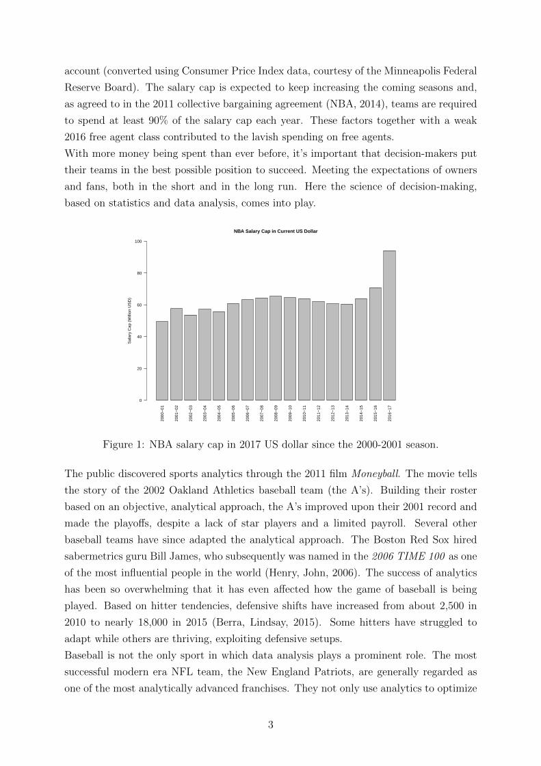
The NBA salary cap increased 34.5% from the 2015-16 season to the 2016-17 season, a
result of increased revenues generated mainly by the nine year, 24 billion dollar media
rights agreements the NBA signed in 2014. The deal kicked in during the 2016 off-season.
The average television revenue increased from 930 million dollar per year to 2.67 billion
dollar (Berger, Ken, 2016). Figure 1 depicts the evolution of the salary cap in 2017
US dollar since the 2000-01 season (Sports Reference LLC, 2017c), taking inflation into
2
Page 9
account (converted using Consumer Price Index data, courtesy of the Minneapolis Federal
Reserve Board). The salary cap is expected to keep increasing the coming seasons and,
as agreed to in the 2011 collective bargaining agreement (NBA, 2014), teams are required
to spend at least 90% of the salary cap each year. These factors together with a weak
2016 free agent class contributed to the lavish spending on free agents.
With more money being spent than ever before, it’s important that decision-makers put
their teams in the best possible position to succeed. Meeting the expectations of owners
and fans, both in the short and in the long run. Here the science of decision-making,
based on statistics and data analysis, comes into play.
2000
−01
2001
−02
2002
−03
2003
−04
2004
−05
2005
−06
2006
−07
2007
−08
2008
−09
2009
−10
2010
−11
2011
−12
2012
−13
2013
−14
2014
−15
2015
−16
2016
−17
NBA Salary Cap in Current US Dollar
Sal
ary
Cap
(M
illio
n U
SD
)
0
20
40
60
80
100
Figure 1: NBA salary cap in 2017 US dollar since the 2000-2001 season.
The public discovered sports analytics through the 2011 film Moneyball. The movie tells
the story of the 2002 Oakland Athletics baseball team (the A’s). Building their roster
based on an objective, analytical approach, the A’s improved upon their 2001 record and
made the playoffs, despite a lack of star players and a limited payroll. Several other
baseball teams have since adapted the analytical approach. The Boston Red Sox hired
sabermetrics guru Bill James, who subsequently was named in the 2006 TIME 100 as one
of the most influential people in the world (Henry, John, 2006). The success of analytics
has been so overwhelming that it has even affected how the game of baseball is being
played. Based on hitter tendencies, defensive shifts have increased from about 2,500 in
2010 to nearly 18,000 in 2015 (Berra, Lindsay, 2015). Some hitters have struggled to
adapt while others are thriving, exploiting defensive setups.
Baseball is not the only sport in which data analysis plays a prominent role. The most
successful modern era NFL team, the New England Patriots, are generally regarded as
one of the most analytically advanced franchises. They not only use analytics to optimize
3
Page 10
their payroll, but also to make data driven play-calling decisions on the field. One of the
worst modern era NFL teams, the Cleveland Browns, recently hired analytics expert Paul
DePodesta away from the New York Mets in the hope of turning their franchise around.
In soccer, the English Premier League team Arsenal outright bought a sports analytics
company to avoid them working for their rivals (Smith, Rory, 2017). These days, almost
every professional sports team either has an analytics department or analytics experts on
their staff with the goal of creating a competitive advantage.
With the growing interest in sports analytics, scientific research in this field has also
grown. Several scientists are collaborating on the subject, resulting in multiple research
groups and projects such as BDSports (bodai.unibs.it/BDSports) and MathSport In-
ternational (www.mathsportinternational.com).
Data of a basketball game is compiled in the so-called box score, which includes several
statistics. In February 2013, the NBA announced the launch of NBA.com/Stats (NBA
Communications, 2013a), making the entire official statistics history available to the pub-
lic. The NBA was the first major U.S. professional sports league to install player tracking
technology in 2009 for certain games. Starting from the 2013-14 season (NBA Communi-
cations, 2013b), the movement of the ball and of all players on the court were measured
in every game, introducing the era of big data in basketball. Basketball analysis and pre-
diction have been the subject of several Kaggle competitions. A competition was held to
predict the probability of Kobe Bryant making certain field goals, based on shot selection.
There is also a yearly March Machine Learning Mania tournament to predict the proba-
bility of teams winning games in the NCAA Division I Men’s Basketball Tournament.
Kubatko, Oliver, Pelton, and Rosenbaum (2007) published an overview of what today are
considered the basics of basketball analytics. Central to their analysis is the concept of
possessions. A possession is defined as starting when a team gains control of the basket-
ball and ending when that team gives up control of the basketball. An offensive rebound
thus extends a possession rather than starting a new one. With this definition, the two
teams in a game have about the same amount of possessions and the team being more
efficient per possession usually wins the game. Possessions therefore are a useful measure
to evaluate the efficiency of teams, especially between games. A team that scores less
points per game on average might do so more efficiently than a team that scores more
points per game on average but plays at a higher pace. Pace is defined as the number of
possessions per 48 minutes by a NBA team. Since possessions are not an officially mea-
sured statistic, Kubatko et al. (2007) provide a formula to estimate possessions from the
box score. The evaluations of efficiency are called offensive rating and defensive rating,
being the average amount of points scored and given up respectively per 100 possessions.
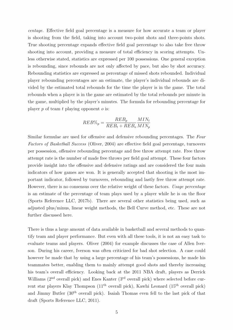
Two other important concepts are effective field goal percentage and true shooting per-
4
Page 11
centage. Effective field goal percentage is a measure for how accurate a team or player
is shooting from the field, taking into account two-point shots and three-points shots.
True shooting percentage expands effective field goal percentage to also take free throw
shooting into account, providing a measure of total efficiency in scoring attempts. Un-
less otherwise stated, statistics are expressed per 100 possessions. One general exception
is rebounding, since rebounds are not only affected by pace, but also by shot accuracy.
Rebounding statistics are expressed as percentage of missed shots rebounded. Individual
player rebounding percentages are an estimate, the player’s individual rebounds are di-
vided by the estimated total rebounds for the time the player is in the game. The total
rebounds when a player is in the game are estimated by the total rebounds per minute in
the game, multiplied by the player’s minutes. The formula for rebounding percentage for
player p of team t playing opponent o is:
REB%p =REBp
REBt + REBo
MINt
MINp
Similar formulae are used for offensive and defensive rebounding percentages. The Four
Factors of Basketball Success (Oliver, 2004) are effective field goal percentage, turnovers
per possession, offensive rebounding percentage and free throw attempt rate. Free throw
attempt rate is the number of made free throws per field goal attempt. These four factors
provide insight into the offensive and defensive ratings and are considered the four main
indicators of how games are won. It is generally accepted that shooting is the most im-
portant indicator, followed by turnovers, rebounding and lastly free throw attempt rate.
However, there is no consensus over the relative weight of these factors. Usage percentage
is an estimate of the percentage of team plays used by a player while he is on the floor
(Sports Reference LLC, 2017b). There are several other statistics being used, such as
adjusted plus/minus, linear weight methods, the Bell Curve method, etc. These are not
further discussed here.
There is thus a large amount of data available in basketball and several methods to quan-
tify team and player performance. But even with all these tools, it is not an easy task to
evaluate teams and players. Oliver (2004) for example discusses the case of Allen Iver-
son. During his career, Iverson was often criticized for bad shot selection. A case could
however be made that by using a large percentage of his team’s possessions, he made his
teammates better, enabling them to mainly attempt good shots and thereby increasing
his team’s overall efficiency. Looking back at the 2011 NBA draft, players as Derrick
Williams (2nd overall pick) and Enes Kanter (3rd overall pick) where selected before cur-
rent star players Klay Thompson (11th overall pick), Kawhi Leonard (15th overall pick)
and Jimmy Butler (30th overall pick). Isaiah Thomas even fell to the last pick of that
draft (Sports Reference LLC, 2011).
5
Page 12
The difficulty in evaluating basketball is due to intangibles such as work ethic, love of the
game, team chemistry, etc. but also due to the nature of basketball. Being played with
only five players per team, the interaction between players in a team is vital, as are player
matchups and coaching. It is also a fact that most of the publicly available statistics
focus on offense. While there are multiple measures for shooting efficiency, none take into
account the difficulty of a shot. Uncontested shots receive the same weight as the most
difficult, most contested shots. There are no statistics keeping track of which defenders
force their opponents to attempt bad shots.
The first part of this thesis aims to provide an accessible method to provide insight into
the NBA dynamics, exploring how the shooting aspect of the game has evolved in recent
years, which teams and players have similar playing styles and what the impact is of
players changing teams.
A much discussed topic every year is which player should win the NBA most valuable
player (MVP) award. Some reporters make the case for the player they think should win
the award, while others even track down votes. The rules for the 2017 MVP award have
changed, as the voting panel is now made up of independent media members (Rohrbach,
Ben, 2017). Team broadcasters used to be able to cast their votes. The voters elect their
top 5 in order, with players receiving 10, 7, 5, 3 and 1 points respectively.
During the 2016-17 season, Russell Westbrook and James Harden emerged as the top
two candidates to win MVP. Westbrook joined Oscar Robertson as the only players in
league history to average a triple-double for an entire season. He also broke the record
for triple-doubles in a season with 42 and led his team to the sixth place in the Western
Conference. He did all this despite losing Kevin Durant in the off-season. Harden led
his team to the third place in the Western Conference, improving their winning record
from 0.500 in 2016 to 0.671 in 2017. He had a higher effective field goal percentage than
Westbrook. However, Westbrook averaged more rebounds per game and per 100 posses-
sions. Both players carried their team to the playoffs without other star players in their
supporting cast. Interestingly, Russell Westbrook was only voted a reserve for the 2017
All-Star game. The second part of this thesis investigates whether the MVP voting can
be modelled and predicted for the upcoming 2017 voting.
Another much discussed aspect of basketball is forecasting the outcome of games. Several
methods have been attempted to outperform the experts and the betting market, in-
cluding a dynamic, time-varying approach (Manner, 2016), neural networks (Loeffelholz,
Bednar, & Bauer, 2009) and other machine learning techniques (Cheng, Dade, Lipman,
& Mills, 2013).
Feustel and Howard (2010) make a case that sports wagering is very similar to investing
6
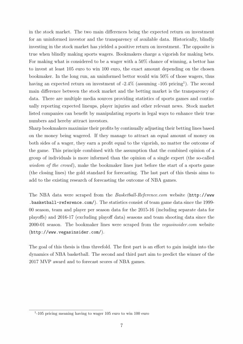
Page 13
in the stock market. The two main differences being the expected return on investment
for an uninformed investor and the transparency of available data. Historically, blindly
investing in the stock market has yielded a positive return on investment. The opposite is
true when blindly making sports wagers. Bookmakers charge a vigorish for making bets.
For making what is considered to be a wager with a 50% chance of winning, a bettor has
to invest at least 105 euro to win 100 euro, the exact amount depending on the chosen
bookmaker. In the long run, an uninformed bettor would win 50% of those wagers, thus
having an expected return on investment of -2.4% (assuming -105 pricing1). The second
main difference between the stock market and the betting market is the transparency of
data. There are multiple media sources providing statistics of sports games and contin-
ually reporting expected lineups, player injuries and other relevant news. Stock market
listed companies can benefit by manipulating reports in legal ways to enhance their true
numbers and hereby attract investors.
Sharp bookmakers maximize their profits by continually adjusting their betting lines based
on the money being wagered. If they manage to attract an equal amount of money on
both sides of a wager, they earn a profit equal to the vigorish, no matter the outcome of
the game. This principle combined with the assumption that the combined opinion of a
group of individuals is more informed than the opinion of a single expert (the so-called
wisdom of the crowd), make the bookmaker lines just before the start of a sports game
(the closing lines) the gold standard for forecasting. The last part of this thesis aims to
add to the existing research of forecasting the outcome of NBA games.
The NBA data were scraped from the Basketball-Reference.com website (http://www
.basketball-reference.com/). The statistics consist of team game data since the 1999-
00 season, team and player per season data for the 2015-16 (including separate data for
playoffs) and 2016-17 (excluding playoff data) seasons and team shooting data since the
2000-01 season. The bookmaker lines were scraped from the vegasinsider.com website
(http://www.vegasinsider.com/).
The goal of this thesis is thus threefold. The first part is an effort to gain insight into the
dynamics of NBA basketball. The second and third part aim to predict the winner of the
2017 MVP award and to forecast scores of NBA games.
1-105 pricing meaning having to wager 105 euro to win 100 euro
7
Page 14
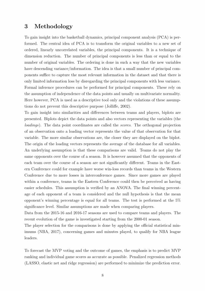
3 Methodology
To gain insight into the basketball dynamics, principal component analysis (PCA) is per-
formed. The central idea of PCA is to transform the original variables to a new set of
ordered, linearly uncorrelated variables, the principal components. It is a technique of
dimension reduction. The number of principal components is less than or equal to the
number of original variables. The ordering is done in such a way that the new variables
have descending variance/information. The idea is that a small number of principal com-
ponents suffice to capture the most relevant information in the dataset and that there is
only limited information loss by disregarding the principal components with less variance.
Formal inference procedures can be performed for principal components. These rely on
the assumption of independence of the data points and usually on multivariate normality.
Here however, PCA is used as a descriptive tool only and the violations of these assump-
tions do not prevent this descriptive purpose (Jolliffe, 2002).
To gain insight into similarities and differences between teams and players, biplots are
presented. Biplots depict the data points and also vectors representing the variables (the
loadings). The data point coordinates are called the scores. The orthogonal projection
of an observation onto a loading vector represents the value of that observation for that
variable. The more similar observations are, the closer they are displayed on the biplot.
The origin of the loading vectors represents the average of the database for all variables.
An underlying assumption is that these comparisons are valid. Teams do not play the
same opponents over the course of a season. It is however assumed that the opponents of
each team over the course of a season are not significantly different. Teams in the East-
ern Conference could for example have worse win-loss records than teams in the Western
Conference due to more losses in interconference games. Since more games are played
within a conference, teams in the Eastern Conference could then be perceived as having
easier schedules. This assumption is verified by an ANOVA. The final winning percent-
age of each opponent of a team is considered and the null hypothesis is that the mean
opponent’s winning percentage is equal for all teams. The test is performed at the 5%
significance level. Similar assumptions are made when comparing players.
Data from the 2015-16 and 2016-17 seasons are used to compare teams and players. The
recent evolution of the game is investigated starting from the 2000-01 season.
The player selection for the comparisons is done by applying the official statistical min-
imums (NBA, 2017), concerning games and minutes played, to qualify for NBA league
leaders.
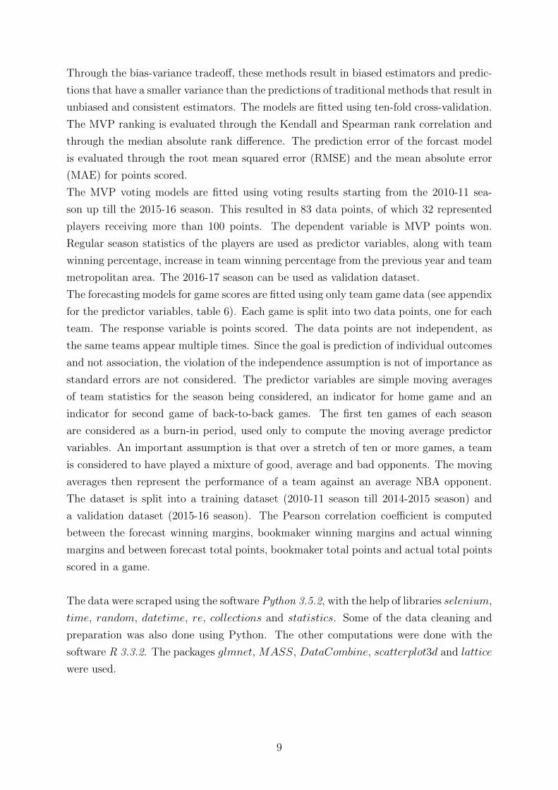
To forecast the MVP voting and the outcome of games, the emphasis is to predict MVP
ranking and individual game scores as accurate as possible. Penalized regression methods
(LASSO, elastic net and ridge regression) are performed to minimize the prediction error.
8
Page 15
Through the bias-variance tradeoff, these methods result in biased estimators and predic-
tions that have a smaller variance than the predictions of traditional methods that result in
unbiased and consistent estimators. The models are fitted using ten-fold cross-validation.
The MVP ranking is evaluated through the Kendall and Spearman rank correlation and
through the median absolute rank difference. The prediction error of the forcast model
is evaluated through the root mean squared error (RMSE) and the mean absolute error
(MAE) for points scored.
The MVP voting models are fitted using voting results starting from the 2010-11 sea-
son up till the 2015-16 season. This resulted in 83 data points, of which 32 represented
players receiving more than 100 points. The dependent variable is MVP points won.
Regular season statistics of the players are used as predictor variables, along with team
winning percentage, increase in team winning percentage from the previous year and team
metropolitan area. The 2016-17 season can be used as validation dataset.
The forecasting models for game scores are fitted using only team game data (see appendix
for the predictor variables, table 6). Each game is split into two data points, one for each
team. The response variable is points scored. The data points are not independent, as
the same teams appear multiple times. Since the goal is prediction of individual outcomes
and not association, the violation of the independence assumption is not of importance as
standard errors are not considered. The predictor variables are simple moving averages
of team statistics for the season being considered, an indicator for home game and an
indicator for second game of back-to-back games. The first ten games of each season
are considered as a burn-in period, used only to compute the moving average predictor
variables. An important assumption is that over a stretch of ten or more games, a team
is considered to have played a mixture of good, average and bad opponents. The moving
averages then represent the performance of a team against an average NBA opponent.
The dataset is split into a training dataset (2010-11 season till 2014-2015 season) and
a validation dataset (2015-16 season). The Pearson correlation coefficient is computed
between the forecast winning margins, bookmaker winning margins and actual winning
margins and between forecast total points, bookmaker total points and actual total points
scored in a game.
The data were scraped using the software Python 3.5.2, with the help of libraries selenium,
time, random, datetime, re, collections and statistics. Some of the data cleaning and
preparation was also done using Python. The other computations were done with the
software R 3.3.2. The packages glmnet, MASS, DataCombine, scatterplot3d and lattice
were used.
9
Page 16
4 Results and Discussion
The available shot location data groups shot selection (% of shots) and scoring percentages
(FG%) based on distance. There are five classes and thus ten variables:
• 0 to 3 feet from the basket;
• 3 to 10 feet from the basket;
• 10 to 16 feet from the basket;
• 2-point shots from more than 16 feet;
• 3-point shots.
The other statistics being considered are pace, free throw percentage (FT%), offensive
and defensive rebounding percentage (Off and Def RB%), usage percentage (USG%), true
shooting percentage (TS%), three-point attempt rate (3PAr) and free throw attempt rate
(FTr). Team assists (AST), steals (STL), blocks (BLK), turnovers (TOV) and personal
fouls (PF) are presented per 100 possessions. For players, assists (AST%), steals (STL%),
blocks (BLK%) and turnovers (TOV%) are expressed as percentages. Teams and players
are often ranked according to offensive (Off Rtg) or defensive rating (Def Rtg). The MVP
criterion also takes more advanced statistics into account.
4.1 Recent Offensive Evolution
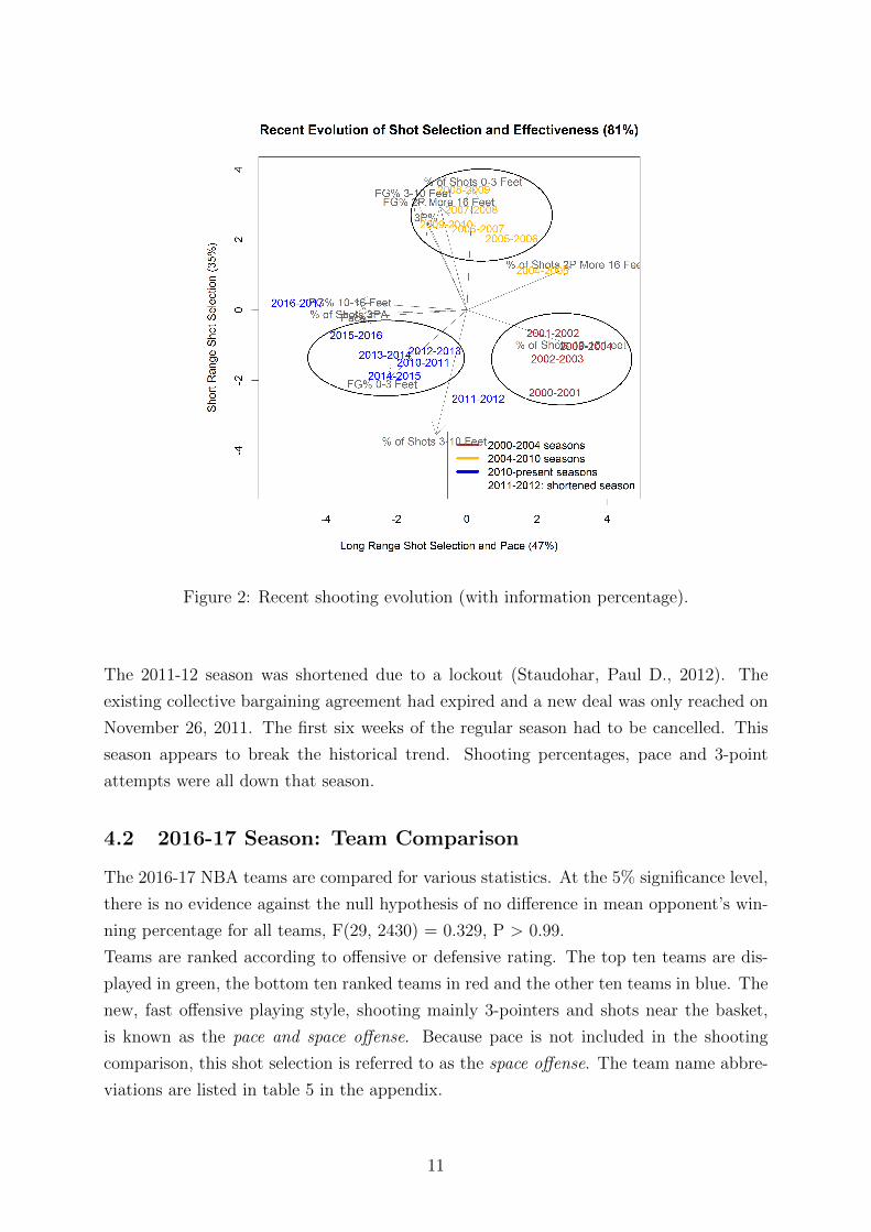
First the recent offensive evolution is discussed. Figure 2 depicts the league average shot
selection and shooting percentages since the 2000-01 season. Over 80% of the information
in the dataset is retained with the first two principal components. In the early 2000 years,
teams preferred to shoot more long 2-pointers. Starting from 2005, the emphasis shifted
towards 3-pointers and away from long 2-point attempts. This shift went hand in hand
with an increase in pace and an increase in shooting percentage for those long 2-pointers.
Another interesting trend is seen starting from 2005. All shooting percentages went up.
This can probably be attributed to the introduction of the rule outlawing hand-checking
above the foul line in 2004 (NBA, 2008). Due to this rule, strong, tall players became
limited in their ability to defend, while guards could play more aggressive and became
more important. The percentage of short shots (0 to 3 feet from the basket) also went up
drastically.
It appears that after several years, the league adapted and the percentage of short shot
attempts (0 to 3 feet from the basket) went down again to the pre-2005 level. Those
short 2-pointers were replaced by mid-range 2-pointers (3 to 10 feet from the basket).
Three-point attempts also kept increasing while long 2-point attempts kept decreasing.
As with the long 2-pointers, the decrease in short 2-point attempts was also paired with
an increase in shooting percentage for those shots. The last two seasons show the surge
in pace and 3-point attempts is ongoing.
10
Page 17
Figure 2: Recent shooting evolution (with information percentage).
The 2011-12 season was shortened due to a lockout (Staudohar, Paul D., 2012). The
existing collective bargaining agreement had expired and a new deal was only reached on
November 26, 2011. The first six weeks of the regular season had to be cancelled. This
season appears to break the historical trend. Shooting percentages, pace and 3-point
attempts were all down that season.
4.2 2016-17 Season: Team Comparison
The 2016-17 NBA teams are compared for various statistics. At the 5% significance level,
there is no evidence against the null hypothesis of no difference in mean opponent’s win-
ning percentage for all teams, F(29, 2430) = 0.329, P > 0.99.
Teams are ranked according to offensive or defensive rating. The top ten teams are dis-
played in green, the bottom ten ranked teams in red and the other ten teams in blue. The
new, fast offensive playing style, shooting mainly 3-pointers and shots near the basket,
is known as the pace and space offense. Because pace is not included in the shooting
comparison, this shot selection is referred to as the space offense. The team name abbre-
viations are listed in table 5 in the appendix.
11
Page 18
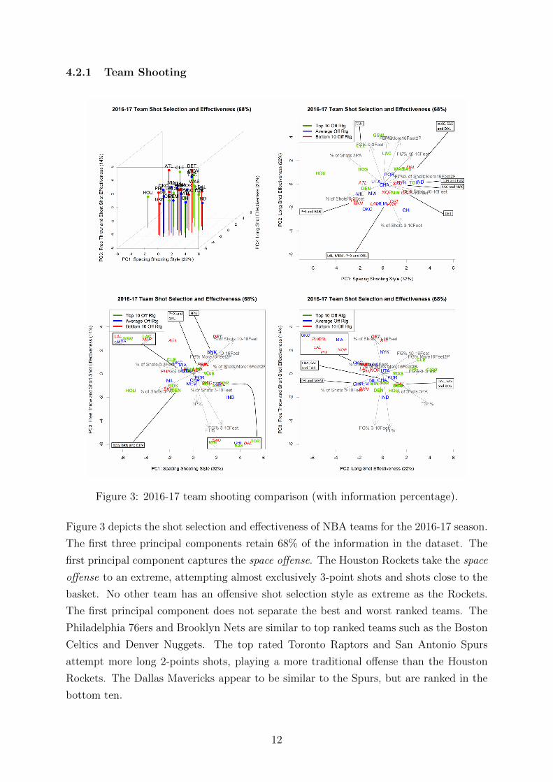
4.2.1 Team Shooting
Figure 3: 2016-17 team shooting comparison (with information percentage).
Figure 3 depicts the shot selection and effectiveness of NBA teams for the 2016-17 season.
The first three principal components retain 68% of the information in the dataset. The
first principal component captures the space offense. The Houston Rockets take the space
offense to an extreme, attempting almost exclusively 3-point shots and shots close to the
basket. No other team has an offensive shot selection style as extreme as the Rockets.
The first principal component does not separate the best and worst ranked teams. The
Philadelphia 76ers and Brooklyn Nets are similar to top ranked teams such as the Boston
Celtics and Denver Nuggets. The top rated Toronto Raptors and San Antonio Spurs
attempt more long 2-points shots, playing a more traditional offense than the Houston
Rockets. The Dallas Mavericks appear to be similar to the Spurs, but are ranked in the
bottom ten.
12
Page 19
The second principal component is a measure for long shot effectiveness. It comes as no
surprise that the best offenses have high marks for long shot effectiveness. The Golden
State Warriors, Cleveland Cavaliers and Los Angeles Clippers excel at 3-point and long
2-point shooting percentages. All top ten rated offenses have average or above average 3-
point scoring percentages. Of those top ten ranked teams, the two teams with the worst
marks for 3-point shooting are the Minnesota Timberwolves and the Denver Nuggets.
Both teams have a Center who is an important part of their offense, Karl-Anthony Towns
for the Timberwolves and Nikola Jokic for the Nuggets. The bottom ranked Dallas Mav-
ericks are rather similar to the top ranked teams. It is also worth noting that three of
the average teams (The Oklahoma City Thunder, Chicago Bulls and Memphis Grizzlies)
have low marks for long shooting effectiveness, being more similar to the bottom ranked
teams.
The third principal component separates teams based on free throw percentage and short
shot effectiveness. The Atlanta Hawks and Detroit Pistons differ from other teams. This
is probably due to their Centers, Dwight Howard and Andre Drummond respectively,
being inept free throw shooters.
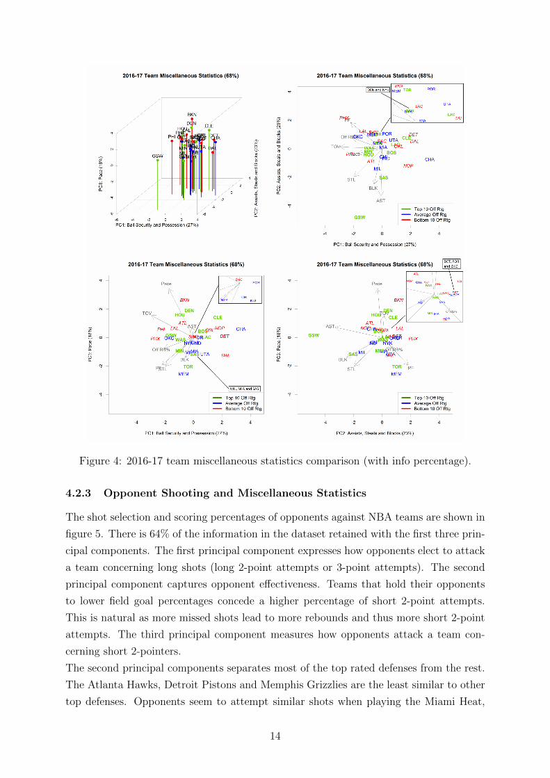
4.2.2 Team Miscellaneous Statistics
To capture 68% of the information of the miscellaneous statistics, three principal compo-
nents are needed. The comparison is shown in figure 4. The first component measures ball
security and extending possessions. Top and bottom ranked teams do not have distinct
patterns. This also holds for the second principal component, expressing assists, steals
and blocks, and the third principal component which expresses pace. The Golden State
Warriors excel at assists, steals and blocks compared to the other teams.
While the Dallas Mavericks and San Antonio Spurs have similar shooting styles, they
do differ concerning possessions and ball security. The Spurs have a higher offensive re-
bounding percentage and also more assists and blocks per 100 possessions. They play at
a slightly higher pace, but also commit more turnovers.
13
Page 20
Figure 4: 2016-17 team miscellaneous statistics comparison (with info percentage).
4.2.3 Opponent Shooting and Miscellaneous Statistics
The shot selection and scoring percentages of opponents against NBA teams are shown in
figure 5. There is 64% of the information in the dataset retained with the first three prin-
cipal components. The first principal component expresses how opponents elect to attack
a team concerning long shots (long 2-point attempts or 3-point attempts). The second
principal component captures opponent effectiveness. Teams that hold their opponents
to lower field goal percentages concede a higher percentage of short 2-point attempts.
This is natural as more missed shots lead to more rebounds and thus more short 2-point
attempts. The third principal component measures how opponents attack a team con-
cerning short 2-pointers.
The second principal components separates most of the top rated defenses from the rest.
The Atlanta Hawks, Detroit Pistons and Memphis Grizzlies are the least similar to other
top defenses. Opponents seem to attempt similar shots when playing the Miami Heat,
14
Page 21
Figure 5: 2016-17 opponent shooting comparison (with information percentage).
Utah Jazz and San Antonio Spurs. Those teams also hold their opponents to compara-
ble scoring percentages. Equivalent conclusions are reached when comparing the Golden
State Warriors and Oklahoma City Thunder. The opponent miscellaneous statistics do
not show any interesting patterns and are not displayed.
4.3 2016-17 Season: Player Comparison
The 2016-17 NBA players are now compared per position. The top five and bottom five
players per position are depicted in green and red respectively. Other players are shown in
blue. The Power Forward and Shooting Guard comparisons do not display any interesting
trends and are not discussed.
15
Page 22
4.3.1 Centers
The first principal component captures 44% of the shooting information and represents
the shooting style of the Centers. As seen in figure 6, there is a difference between the
traditional Centers, playing near the basket, and the more modern Centers, who also
attempt longer shots. Four of the five top rated Centers have a traditional style. This is
not surprising as they attempt shots with higher scoring percentages and are in position
to grab more rebounds. The top rated Center despite his modern style is Nikola Jokic. It
is interesting to see that Clint Capela and Dwight Howard have similar shooting styles.
The Houston Rockets had a bad year in 2016 with Howard and there were rumours that
Harden and Howard, the two stars of that teams, were unable to play with each other.
The Rockets had more success in 2017 with Capela. Andre Drummond and Bismack
Biyombo are among the bottom rated Centers. This is remarkable because they have
a more traditional shooting style. The offensive rating formula should favor traditional
Centers because they usually have higher true shooting percentages and are in position
to grab more rebounds.
Figure 6: 2016-17 shooting comparison of Centers (with information percentage).
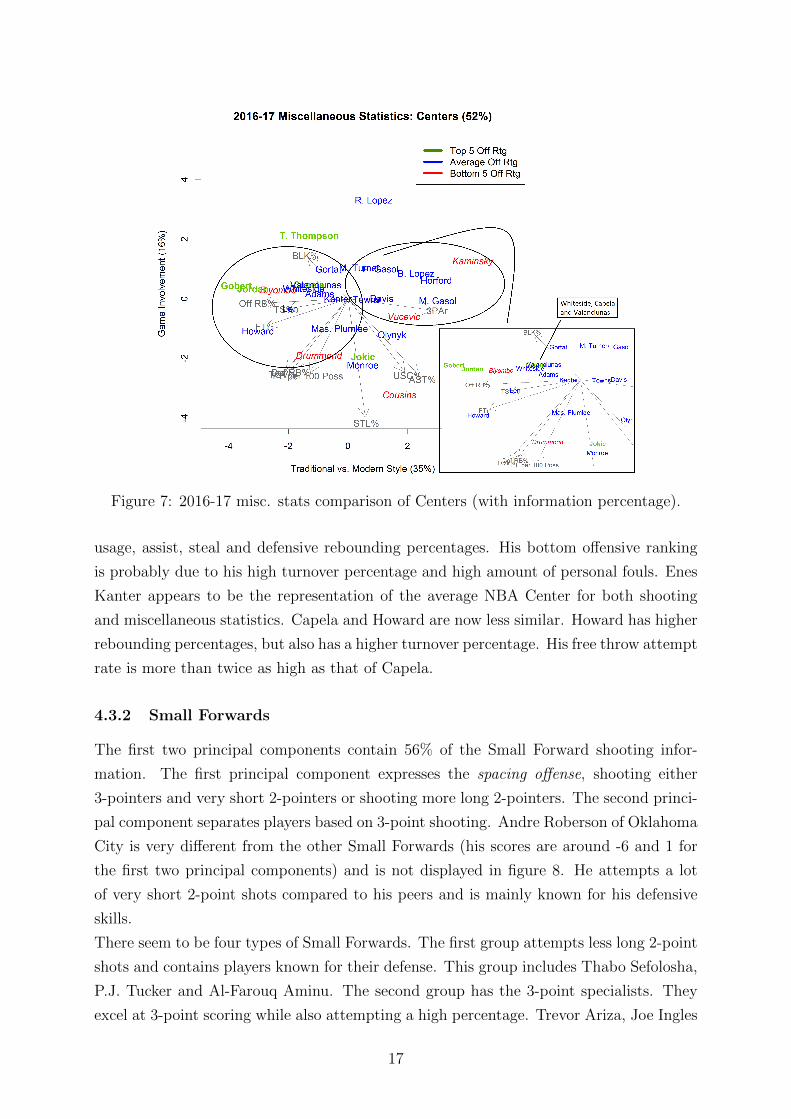
The first principal component of the miscellaneous statistics, shown in figure 7, again
separates the traditional and more modern Centers. The differences are smaller, as the
first component only captures 35% of the variation. As expected, the more traditional
Centers have higher rebounding and blocking percentages. DeMarcus Cousins has high
16
Page 23
Figure 7: 2016-17 misc. stats comparison of Centers (with information percentage).
usage, assist, steal and defensive rebounding percentages. His bottom offensive ranking
is probably due to his high turnover percentage and high amount of personal fouls. Enes
Kanter appears to be the representation of the average NBA Center for both shooting
and miscellaneous statistics. Capela and Howard are now less similar. Howard has higher
rebounding percentages, but also has a higher turnover percentage. His free throw attempt
rate is more than twice as high as that of Capela.
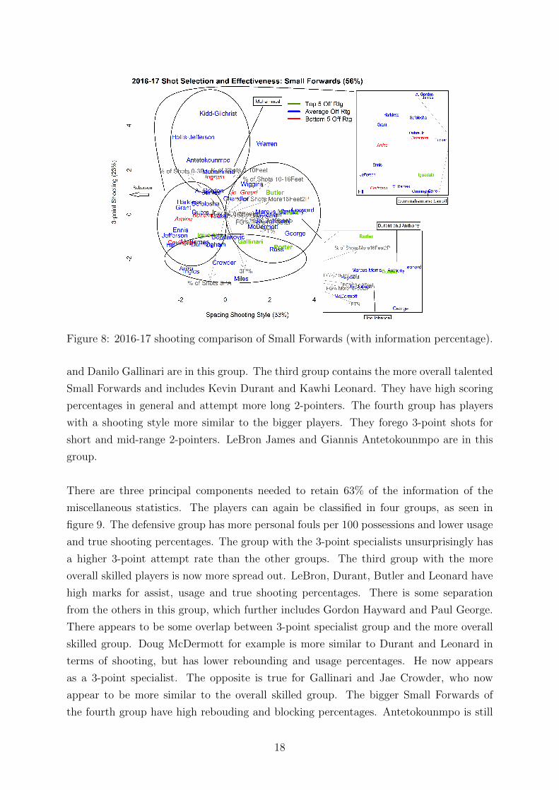
4.3.2 Small Forwards
The first two principal components contain 56% of the Small Forward shooting infor-
mation. The first principal component expresses the spacing offense, shooting either
3-pointers and very short 2-pointers or shooting more long 2-pointers. The second princi-
pal component separates players based on 3-point shooting. Andre Roberson of Oklahoma
City is very different from the other Small Forwards (his scores are around -6 and 1 for
the first two principal components) and is not displayed in figure 8. He attempts a lot
of very short 2-point shots compared to his peers and is mainly known for his defensive
skills.
There seem to be four types of Small Forwards. The first group attempts less long 2-point
shots and contains players known for their defense. This group includes Thabo Sefolosha,
P.J. Tucker and Al-Farouq Aminu. The second group has the 3-point specialists. They
excel at 3-point scoring while also attempting a high percentage. Trevor Ariza, Joe Ingles
17
Page 24
Figure 8: 2016-17 shooting comparison of Small Forwards (with information percentage).
and Danilo Gallinari are in this group. The third group contains the more overall talented
Small Forwards and includes Kevin Durant and Kawhi Leonard. They have high scoring
percentages in general and attempt more long 2-pointers. The fourth group has players
with a shooting style more similar to the bigger players. They forego 3-point shots for
short and mid-range 2-pointers. LeBron James and Giannis Antetokounmpo are in this
group.
There are three principal components needed to retain 63% of the information of the
miscellaneous statistics. The players can again be classified in four groups, as seen in
figure 9. The defensive group has more personal fouls per 100 possessions and lower usage
and true shooting percentages. The group with the 3-point specialists unsurprisingly has
a higher 3-point attempt rate than the other groups. The third group with the more
overall skilled players is now more spread out. LeBron, Durant, Butler and Leonard have
high marks for assist, usage and true shooting percentages. There is some separation
from the others in this group, which further includes Gordon Hayward and Paul George.
There appears to be some overlap between 3-point specialist group and the more overall
skilled group. Doug McDermott for example is more similar to Durant and Leonard in
terms of shooting, but has lower rebounding and usage percentages. He now appears
as a 3-point specialist. The opposite is true for Gallinari and Jae Crowder, who now
appear to be more similar to the overall skilled group. The bigger Small Forwards of
the fourth group have high rebouding and blocking percentages. Antetokounmpo is still
18
Page 25
Figure 9: 2016-17 misc. stats comparison of Small Forwards (with info perc.).
similar to the bigger Small Forwards. He also has very high marks for assist, usage and
true shooting percentages and is therefore also comparable to other star players LeBron,
Durant, Leonard and Butler for miscellaneous statistics.
4.3.3 Point Guards
The main shooting differences between Point Guards are depicted in figure 10 and are
determined by shot selection. The first principal component separates 3-point shooters
and driving Point Guards. These differences make up 27% of the shooting variation. The
next 20% in variation is explained by long 2-point effectiveness. The shooting style of the
undrafted T.J. McConnell is similar to that of 2011 MVP Derrick Rose. Patty Mills has a
style that resembles the one of Stephen Curry, attempting and scoring mostly 3-pointers.
19
Page 26
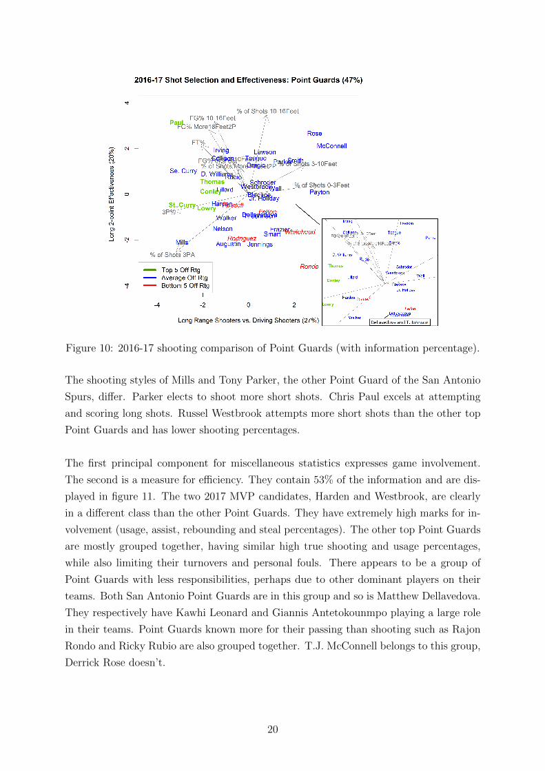
Figure 10: 2016-17 shooting comparison of Point Guards (with information percentage).
The shooting styles of Mills and Tony Parker, the other Point Guard of the San Antonio
Spurs, differ. Parker elects to shoot more short shots. Chris Paul excels at attempting
and scoring long shots. Russel Westbrook attempts more short shots than the other top
Point Guards and has lower shooting percentages.
The first principal component for miscellaneous statistics expresses game involvement.
The second is a measure for efficiency. They contain 53% of the information and are dis-
played in figure 11. The two 2017 MVP candidates, Harden and Westbrook, are clearly
in a different class than the other Point Guards. They have extremely high marks for in-
volvement (usage, assist, rebounding and steal percentages). The other top Point Guards
are mostly grouped together, having similar high true shooting and usage percentages,
while also limiting their turnovers and personal fouls. There appears to be a group of
Point Guards with less responsibilities, perhaps due to other dominant players on their
teams. Both San Antonio Point Guards are in this group and so is Matthew Dellavedova.
They respectively have Kawhi Leonard and Giannis Antetokounmpo playing a large role
in their teams. Point Guards known more for their passing than shooting such as Rajon
Rondo and Ricky Rubio are also grouped together. T.J. McConnell belongs to this group,
Derrick Rose doesn’t.
20
Page 27
Figure 11: 2016-17 misc. stats comparison of Point Guards (with information percentage).
4.4 The Impact of Changing Teams
The impact of a player changing teams is examined. First Golden State and Oklahoma
City are studied before and after Kevin Durant joined the Warriors. Golden State is next
compared to Dallas, in an effort the discover the effect of the teams exchanging Centers.
Lastly, the impact of the DeMarcus Cousins trade is discussed.
4.4.1 Kevin Durant
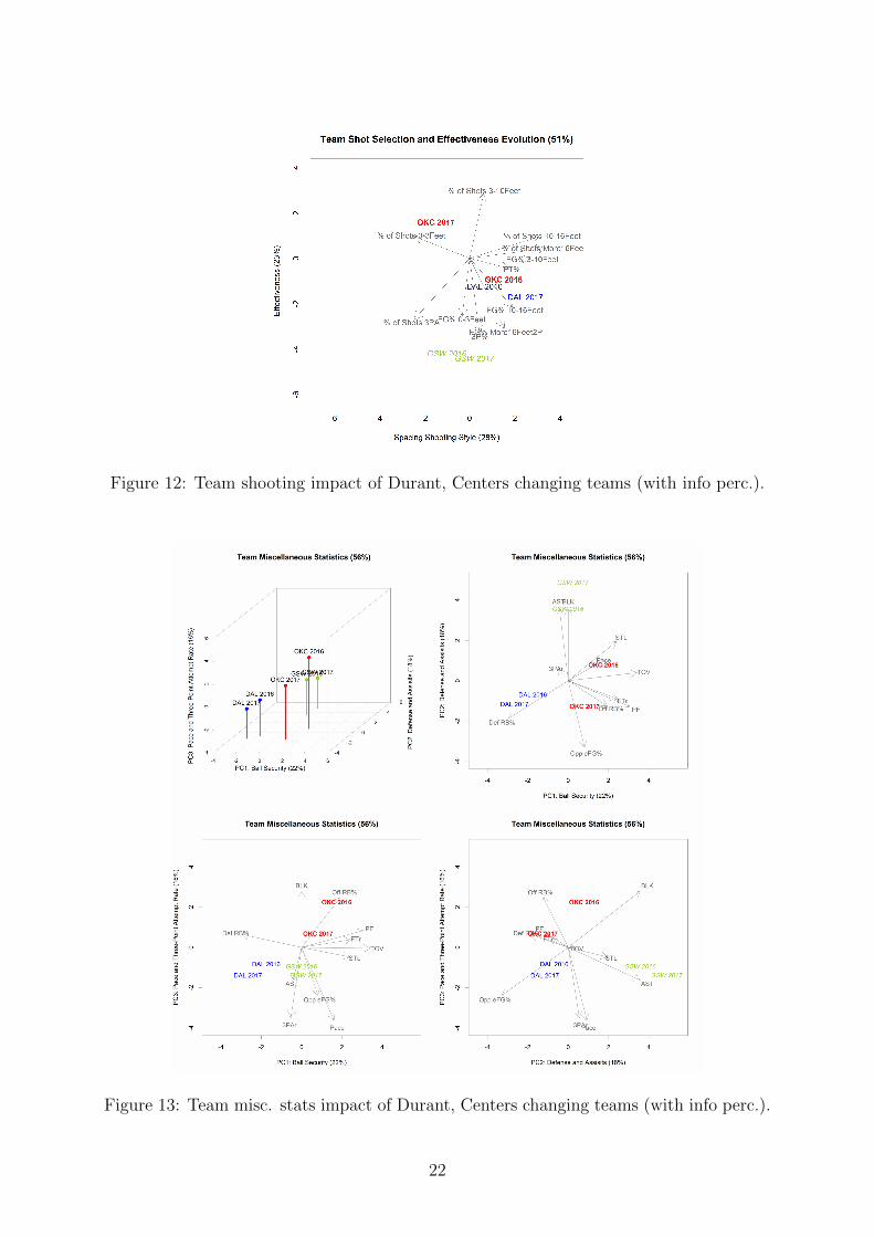
Figure 12 shows that the Oklahoma City Thunder were more affected by losing Kevin
Durant than the Golden State Warriors were by adding him. Golden State attempted
slightly more long 2-point shots in 2017 than in 2016. These shots mainly replaced short
2-point attempts. The Thunder had a big drop in shooting percentage and in long 2-points
attempts. The long 2-point shots were replaced by 3-point and short 2-point attempts.
It is remarkable that the Thunder’s shooting percentage for long 2-pointers decreased
despite attempting less. Usually attempting less shots means taking better shots and
thus an increase in scoring percentage. This does not hold for Oklahoma City and is
likely due to replacing Durant with less good players.
21
Page 28
Figure 12: Team shooting impact of Durant, Centers changing teams (with info perc.).
Figure 13: Team misc. stats impact of Durant, Centers changing teams (with info perc.).
22
Page 29
When considering the miscellaneous statistics depicted in figure 13, both teams seem to be
heading in opposite directions. This is mainly because the Warriors had a lower defensive
rebounding percentage in 2017, but more assists and blocks. A reverse trend is seen for
the Thunder.
Figure 14: Player shooting impact of Durant changing teams (with info percentage).
As seen in figure 14, Golden State star players Stephen Curry, Klay Thompson and Dray-
mond Green have similar shot selection and effectiveness before and after the addition of
Durant. Green had a dip in scoring percentage for mid-range shots in 2017, but those
made up only a small percentage of his attempts. Durant himself was also barely affected
by changing teams. He did attempt more long 2-pointers than the player he replaced,
Harrison Barnes, and was more effective doing so. There were differences between Centers
Andrew Bogut and Zaza Pachulia, but these are discussed later.
Center Steven Adams of Oklahoma City does seem to be somewhat impacted. While he
appears to be taking more short shots, he actually attempted more long shots and his
shooting percentage decreased. Some of this information is lost by retaining only the first
two principal components. The decrease in scoring percentage for Thunder player Andre
Robertson in 2017 is also lost, his higher amount of 3-point attempts on the other hand
is not. Enes Kanter appears to be similar for both years and so are Dion Waiters and his
replacement, Victor Oladipo. This is not the case for Serge Ibaka and his replacement,
Domantas Sabonis. Sabonis attempted less long 2-pointers and had a lower shooting per-
23
Page 30
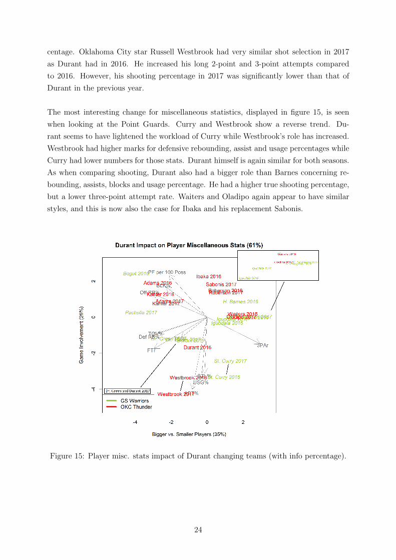
centage. Oklahoma City star Russell Westbrook had very similar shot selection in 2017
as Durant had in 2016. He increased his long 2-point and 3-point attempts compared
to 2016. However, his shooting percentage in 2017 was significantly lower than that of
Durant in the previous year.
The most interesting change for miscellaneous statistics, displayed in figure 15, is seen
when looking at the Point Guards. Curry and Westbrook show a reverse trend. Du-
rant seems to have lightened the workload of Curry while Westbrook’s role has increased.
Westbrook had higher marks for defensive rebounding, assist and usage percentages while
Curry had lower numbers for those stats. Durant himself is again similar for both seasons.
As when comparing shooting, Durant also had a bigger role than Barnes concerning re-
bounding, assists, blocks and usage percentage. He had a higher true shooting percentage,
but a lower three-point attempt rate. Waiters and Oladipo again appear to have similar
styles, and this is now also the case for Ibaka and his replacement Sabonis.
Figure 15: Player misc. stats impact of Durant changing teams (with info percentage).
24
Page 31
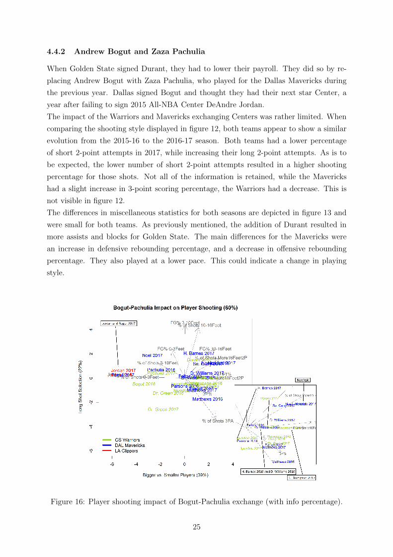
4.4.2 Andrew Bogut and Zaza Pachulia
When Golden State signed Durant, they had to lower their payroll. They did so by re-
placing Andrew Bogut with Zaza Pachulia, who played for the Dallas Mavericks during
the previous year. Dallas signed Bogut and thought they had their next star Center, a
year after failing to sign 2015 All-NBA Center DeAndre Jordan.
The impact of the Warriors and Mavericks exchanging Centers was rather limited. When
comparing the shooting style displayed in figure 12, both teams appear to show a similar
evolution from the 2015-16 to the 2016-17 season. Both teams had a lower percentage
of short 2-point attempts in 2017, while increasing their long 2-point attempts. As is to
be expected, the lower number of short 2-point attempts resulted in a higher shooting
percentage for those shots. Not all of the information is retained, while the Mavericks
had a slight increase in 3-point scoring percentage, the Warriors had a decrease. This is
not visible in figure 12.
The differences in miscellaneous statistics for both seasons are depicted in figure 13 and
were small for both teams. As previously mentioned, the addition of Durant resulted in
more assists and blocks for Golden State. The main differences for the Mavericks were
an increase in defensive rebounding percentage, and a decrease in offensive rebounding
percentage. They also played at a lower pace. This could indicate a change in playing
style.
Figure 16: Player shooting impact of Bogut-Pachulia exchange (with info percentage).
25
Page 32
The impact of the Bogut-Pachulia exchange on the shooting style of individual players is
shown in figure 16. While Bogut appears to have increased his percentage of short shot
attempts with Dallas, in reality there was a shift from very short 2-point attempts (0
to 3 feet from the basket) to short 2-point attempts (3 to 10 feet from the basket). His
field goal percentage for very short shots dropped. This is again not visible on the plot.
It is clear that the Power Forwards for the Mavericks and Warriors have different shoot-
ing styles. Green has a more modern space offense style, attempting mainly very short
2-pointers and 3-pointers. Nowitzki on the other hand has a more traditional style. He
attempted more long 2-pointers and 3-pointers at the cost of short 2-pointers. Pachulia’s
shooting appears quite similar with both Dallas and Golden State. The style of Bogut
with the Mavericks in 2017 was very similar to the style of DeAndre Jordan with the Los
Angeles Clippers.
The Guards of both teams, Curry and Thompson for Golden State and Matthews and
Williams for Dallas, seem to have similar shot selection and effectiveness for both seasons.
The starting Small Forward for Dallas was Chandler Parsons in 2016. He was replaced in
2017 by Harrison Barnes, who played for the Warriors during the previous season. Durant
replaced Barnes. The Small Forwards in 2016 were somewhat similar for both teams. The
same goes for the 2017 season, but both teams had their Small Forward in a different role.
The Small Forwards attempted more long 2-point shots and had higher scoring percent-
ages for those shots. It seems that both Durant for Golden State and Barnes for Dallas
had bigger roles than their predecessors and were more successful.
Most players had similar miscellaneous statistics in 2017 and 2016, as seen in figure 17.
This includes Harrison Barnes who played for different teams. The comparison between
Barnes in Golden State and his successor Kevin Durant leads to the same conclusions as
before. Bogut appears to have had a different role with Dallas than he had with Golden
State, differing more from Pachulia in 2017 than in 2016. Nerlens Noel seems similar to
Pachulia. When comparing DeAndre Jordan and the Dallas version of Andrew Bogut,
both have similar statistics concerning rebounding and blocking. Bogut was less effective
as he had a lower true shooting percentage and more turnovers. He did also have more
assists than Jordan. The change in shot attempts for Bogut in 2017 compared to 2016
has led to a drop in true shooting percentage. He also had more turnovers with Dallas
than the year before with Golden State.
26
Page 33
Figure 17: Player misc. stats impact of Bogut-Pachulia exchange (with info percentage).
4.4.3 DeMarcus Cousins Trade
During the 2017 All-Star break, DeMarcus Cousins was traded from the Sacramento Kings
to the New Orleans Pelicans. Tyreke Evans, Langston Galloway and Buddy Hield joined
the Kings from the Pelicans.
Before the Cousins trade, the Pelicans and Kings had similar shot selection and effective-
ness, as depicted in figure 18. Both teams resembled the league average. The Pelicans
remained close to the league average after adding Cousins. The Kings, on the other
hand, changed their style. They attempted less 3-pointers and short 2-pointers and chose
to shoot more long 2-pointers instead. Shooting less 3-pointers led to a higher 3-point
shooting percentage. Remarkably, even with the increase in attempts, the shooting per-
27
Page 34
Figure 18: Team shooting impact of Cousins trade (with info percentage).
centage for long 2-pointers also increased. The scoring percentage for short 2-point shots
was not affected.
The shooting percentages of opponents against the Pelicans and Kings display different
trends after the trade. The comparison is shown in figure 19. The Kings’ perimeter and
3-point defense improved, but their opponents had higher scoring percentages near the
basket. Opponents increased their mid-range scoring percentage against the Pelicans.
The shot selection against both teams remained rather stable, but this is not clear from
the plots. There were no worthwhile changes in miscellaneous statistics.
Figure 20 depicts the impact of the Cousins trade on the shooting style of the players.
Cousins himself did not seem to be impacted by changing teams. It is interesting to see
that the Pelicans had no players similar to the bigs of the Kings, Koufos and Cauley-Stein,
after the trade. They released their most similar player, Terrence Jones, after acquiring
Cousins. Almost all players of the Kings were impacted by losing Cousins. They all at-
tempted more long 2-pointers and less short 2-pointers. The lone exception was Tolliver,
who attempted more short 2-point shots. McLemore and Temple were the two Kings
players the least affected by the trade.
28
Page 35
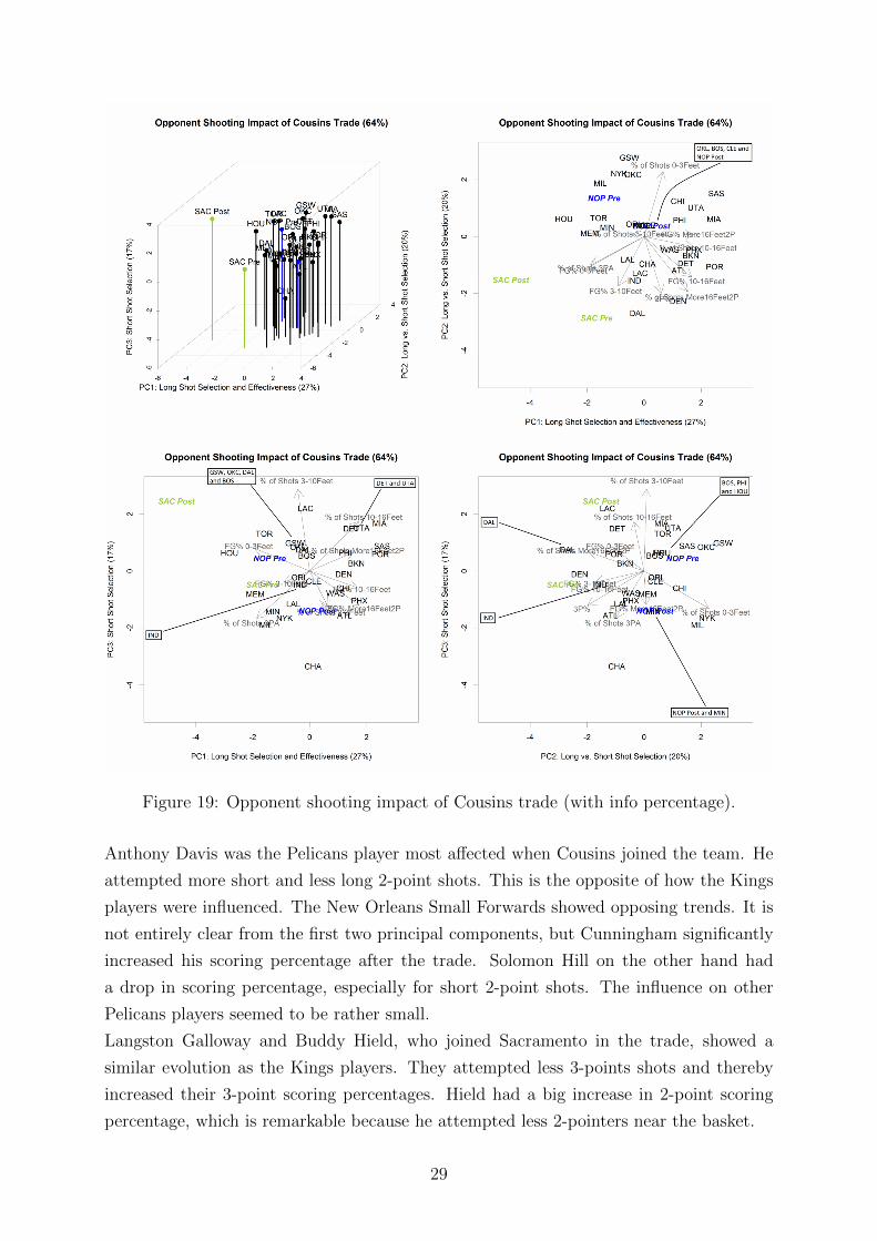
Figure 19: Opponent shooting impact of Cousins trade (with info percentage).
Anthony Davis was the Pelicans player most affected when Cousins joined the team. He
attempted more short and less long 2-point shots. This is the opposite of how the Kings
players were influenced. The New Orleans Small Forwards showed opposing trends. It is
not entirely clear from the first two principal components, but Cunningham significantly
increased his scoring percentage after the trade. Solomon Hill on the other hand had
a drop in scoring percentage, especially for short 2-point shots. The influence on other
Pelicans players seemed to be rather small.
Langston Galloway and Buddy Hield, who joined Sacramento in the trade, showed a
similar evolution as the Kings players. They attempted less 3-points shots and thereby
increased their 3-point scoring percentages. Hield had a big increase in 2-point scoring
percentage, which is remarkable because he attempted less 2-pointers near the basket.
29
Page 36
Figure 20: Player shooting impact of Cousins trade (with info percentage).
The player miscellaneous statistics, displayed in figure 21, show that most players were
not greatly affected by the trade. Evans is the first exception, he saw his assist percentage
drop with his new team, the Kings. He did, however, increase his true shooting percent-
age. The opposite is true for Temple. Temple’s assist, turnover and usage percentages
increased, but his true shooting percentage dropped. Both Cousins and Davis appear to
be more dominant near the basket than the bigs with a more traditional shooting style.
They have higher rebounding and blocking percentages than Koufos, Cauley-Stein and
Jones.
30
Page 37
Figure 21: Player misc. stats impact of Cousins trade (with info percentage).
31
Page 38
4.5 MVP Criterion
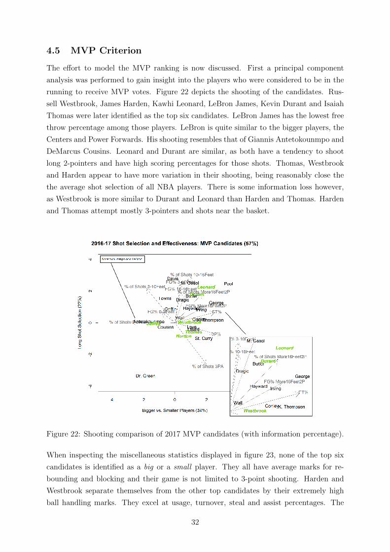
The effort to model the MVP ranking is now discussed. First a principal component
analysis was performed to gain insight into the players who were considered to be in the
running to receive MVP votes. Figure 22 depicts the shooting of the candidates. Rus-
sell Westbrook, James Harden, Kawhi Leonard, LeBron James, Kevin Durant and Isaiah
Thomas were later identified as the top six candidates. LeBron James has the lowest free
throw percentage among those players. LeBron is quite similar to the bigger players, the
Centers and Power Forwards. His shooting resembles that of Giannis Antetokounmpo and
DeMarcus Cousins. Leonard and Durant are similar, as both have a tendency to shoot
long 2-pointers and have high scoring percentages for those shots. Thomas, Westbrook
and Harden appear to have more variation in their shooting, being reasonably close the
the average shot selection of all NBA players. There is some information loss however,
as Westbrook is more similar to Durant and Leonard than Harden and Thomas. Harden
and Thomas attempt mostly 3-pointers and shots near the basket.
Figure 22: Shooting comparison of 2017 MVP candidates (with information percentage).
When inspecting the miscellaneous statistics displayed in figure 23, none of the top six
candidates is identified as a big or a small player. They all have average marks for re-
bounding and blocking and their game is not limited to 3-point shooting. Harden and
Westbrook separate themselves from the other top candidates by their extremely high
ball handling marks. They excel at usage, turnover, steal and assist percentages. The
32
Page 39
high 3-point attempt rate and free throw rate of James Harden is not evident from the
plot. Durant has the highest true shooting percentage of the five. The first three prin-
cipal components do not capture that Westbrook has the lowest true shooting percentage.
Figure 23: Misc. stats comparison of 2017 MVP candidates (with information percentage).
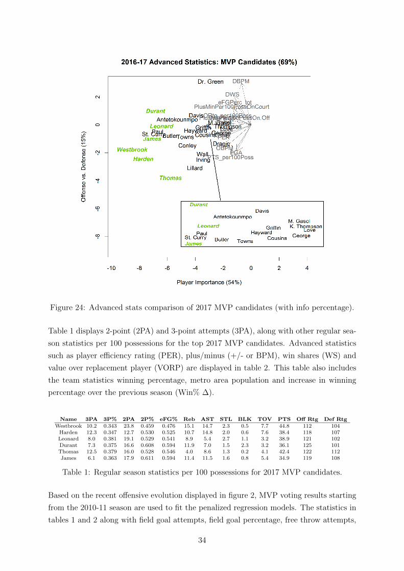
Unsurprisingly, the six players all have good advanced statistics. Figure 24 shows that
there again seems to be a separation between Westbrook and Harden and the other can-
didates. Chris Paul and Stephen Curry have the most similar advanced statistics to the
top candidates. Thomas has the lowest ratings for defensive statistics of the six players.
33
Page 40
Figure 24: Advanced stats comparison of 2017 MVP candidates (with info percentage).
Table 1 displays 2-point (2PA) and 3-point attempts (3PA), along with other regular sea-
son statistics per 100 possessions for the top 2017 MVP candidates. Advanced statistics
such as player efficiency rating (PER), plus/minus (+/- or BPM), win shares (WS) and
value over replacement player (VORP) are displayed in table 2. This table also includes
the team statistics winning percentage, metro area population and increase in winning
percentage over the previous season (Win% ∆).
Name 3PA 3P% 2PA 2P% eFG% Reb AST STL BLK TOV PTS Off Rtg Def RtgWestbrook 10.2 0.343 23.8 0.459 0.476 15.1 14.7 2.3 0.5 7.7 44.8 112 104
Harden 12.3 0.347 12.7 0.530 0.525 10.7 14.8 2.0 0.6 7.6 38.4 118 107Leonard 8.0 0.381 19.1 0.529 0.541 8.9 5.4 2.7 1.1 3.2 38.9 121 102Durant 7.3 0.375 16.6 0.608 0.594 11.9 7.0 1.5 2.3 3.2 36.1 125 101Thomas 12.5 0.379 16.0 0.528 0.546 4.0 8.6 1.3 0.2 4.1 42.4 122 112James 6.1 0.363 17.9 0.611 0.594 11.4 11.5 1.6 0.8 5.4 34.9 119 108
Table 1: Regular season statistics per 100 possessions for 2017 MVP candidates.
Based on the recent offensive evolution displayed in figure 2, MVP voting results starting
from the 2010-11 season are used to fit the penalized regression models. The statistics in
tables 1 and 2 along with field goal attempts, field goal percentage, free throw attempts,
34
Page 41
Name PER USG% Off WS Def WS WS/48 min +/- VORP Win% Metro Area Win% ∆Westbrook 30.6 41.7 8.5 4.6 0.224 15.5 12.4 0.573 1.5 M -0.098
Harden 27.3 34.2 11.5 3.6 0.245 10.1 9.0 0.671 6.3 M 0.171Leonard 27.5 31.1 8.9 4.7 0.264 7.9 6.2 0.744 2.4 M -0.073Durant 27.6 27.8 8.0 4.0 0.278 8.0 5.2 0.817 4.3 M -0.073Thomas 26.5 34.0 10.9 1.6 0.234 5.3 4.8 0.646 4.6 M 0.061James 27.0 30.0 9.8 3.0 0.221 8.4 7.3 0.622 2.1 M -0.073
Table 2: Advanced and team regular season statistics for 2017 MVP candidates.
free throw percentage, personal fouls, true shooting percentage, three-point attempt rate,
free throw rate, plus/minus (on court), plus/minus net and points generated by assists
(PGA) are used as predictor variables. The statistics are per 100 possessions if applicable.
Rebounds and plus/minus are not directly used, but rather split up in offensive and
defensive rebounds and plus/minus.
The dependent variable is MVP points won. Usually three or less players receive the
majority of the top votes and the remaining votes are spread out over several players.
This leads to the difficulty of which conditional distribution to assume for the outcome
variable (conditional on the predictor variables). A gaussian conditional distribution
seems reasonable for the top players, but inappropriate for the others. There, a poisson
conditional distribution seems to be a better fit. Several models are explored and their
performance is compared.
Polynomial models are fitted with both a gaussian and poisson conditional distribution
assumed. Next, linear and polynomial models are fitted after transforming the outcome
variable. Because the outcome variable is right-skewed, a logarithmic transformation
is performed. For each approach, the predictions of the LASSO, elastic net and ridge
regression are averaged to compute the final predicted MVP points. The performance
is compared in table 3. The prediction error is calculated for a ranking of the entire
training dataset, based on actual MVP points and disregarding the separate seasons. The
prediction error is also computed for each separate season and then averaged.
Results disregarding separate seasonsPoly. w/ gaussian Poly. w/ poisson Linear w/ Poly. w/
cond. distr. cond. distr. transf. transf.Kendall’s τ 0.613 0.647 0.677 0.673
Spearman’s ρ 0.792 0.820 0.846 0.843median absolute
difference in ranks 9 7.5 6 6
Averaged per season resultsPoly. w/ gaussian Poly. w/ poisson Linear w/ Poly. w/
cond. distr. cond. distr. transf. transf.Kendall’s τ 0.623 0.635 0.662 0.653
Spearman’s ρ 0.776 0.788 0.808 0.800median absolute
difference in ranks 1.5 1 1.5 1
Table 3: Prediction error of MVP models on training dataset (the mean is reported for theaveraged rank correlation, the median is reported of the median absolute rank differences).
35
Page 42
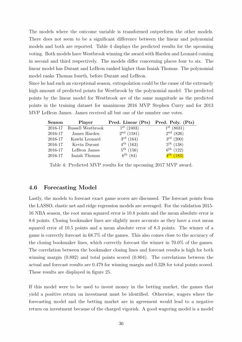
The models where the outcome variable is transformed outperform the other models.
There does not seem to be a significant difference between the linear and polynomial
models and both are reported. Table 4 displays the predicted results for the upcoming
voting. Both models have Westbrook winning the award with Harden and Leonard coming
in second and third respectively. The models differ concerning places four to six. The
linear model has Durant and LeBron ranked higher than Isaiah Thomas. The polynomial
model ranks Thomas fourth, before Durant and LeBron.
Since he had such an exceptional season, extrapolation could be the cause of the extremely
high amount of predicted points for Westbrook by the polynomial model. The predicted
points by the linear model for Westbrook are of the same magnitude as the predicted
points in the training dataset for unanimous 2016 MVP Stephen Curry and for 2013
MVP LeBron James. James received all but one of the number one votes.
Season Player Pred. Linear (Pts) Pred. Poly. (Pts)
2016-17 Russell Westbrook 1st (2403) 1st (8031)2016-17 James Harden 2nd (1581) 2nd (826)2016-17 Kawhi Leonard 3rd (164) 3rd (200)2016-17 Kevin Durant 4th (163) 5th (138)2016-17 LeBron James 5th (156) 6th (122)2016-17 Isaiah Thomas 6th (84) 4th (183)
Table 4: Predicted MVP results for the upcoming 2017 MVP award.
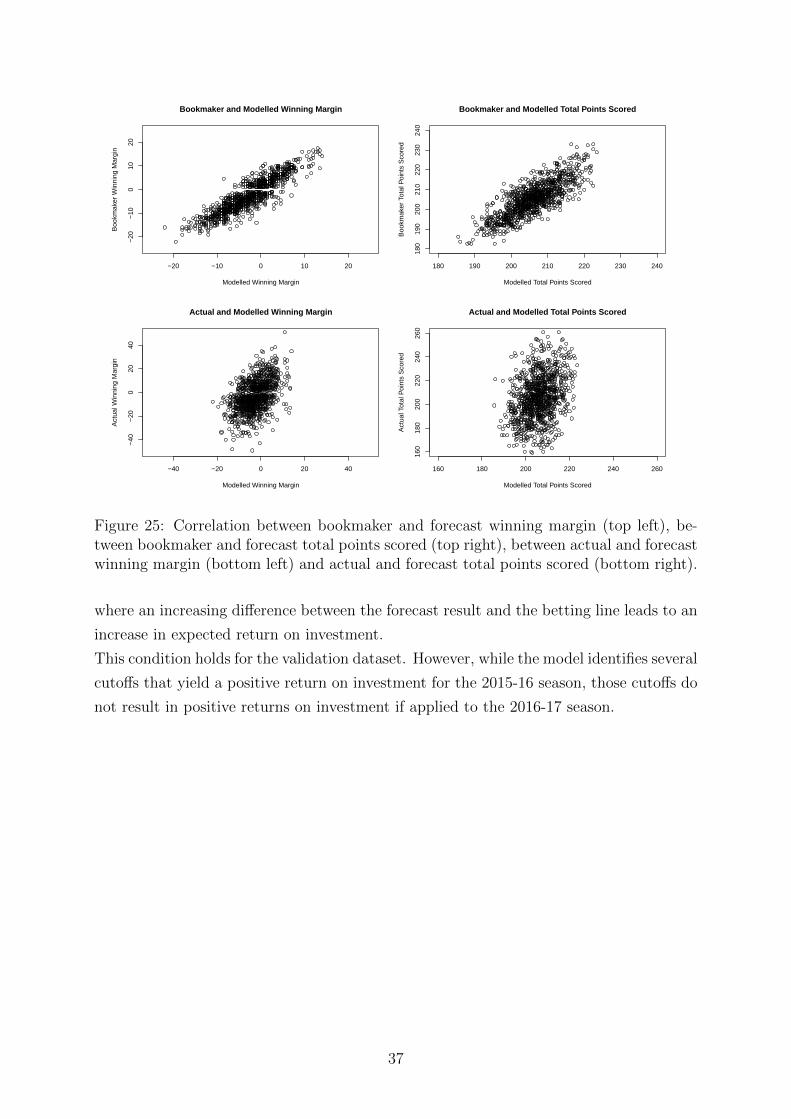
4.6 Forecasting Model
Lastly, the models to forecast exact game scores are discussed. The forecast points from
the LASSO, elastic net and ridge regression models are averaged. For the validation 2015-
16 NBA season, the root mean squared error is 10.8 points and the mean absolute error is
8.6 points. Closing bookmaker lines are slightly more accurate as they have a root mean
squared error of 10.5 points and a mean absolute error of 8.3 points. The winner of a
game is correctly forecast in 68.7% of the games. This also comes close to the accuracy of
the closing bookmaker lines, which correctly forecast the winner in 70.0% of the games.
The correlation between the bookmaker closing lines and forecast results is high for both
winning margin (0.892) and total points scored (0.804). The correlations between the
actual and forecast results are 0.479 for winning margin and 0.328 for total points scored.
These results are displayed in figure 25.
If this model were to be used to invest money in the betting market, the games that
yield a positive return on investment must be identified. Otherwise, wagers where the
forecasting model and the betting market are in agreement would lead to a negative
return on investment because of the charged vigorish. A good wagering model is a model
36
Page 43
−20 −10 0 10 20
−20
−10
010
20
Bookmaker and Modelled Winning Margin
Modelled Winning Margin
Boo
kmak
er W
inni
ng M
argi
n
180 190 200 210 220 230 240
180
190
200
210
220
230
240
Bookmaker and Modelled Total Points Scored
Modelled Total Points Scored
Boo
kmak
er T
otal
Poi
nts
Sco
red
−40 −20 0 20 40
−40
−20
020
40
Actual and Modelled Winning Margin
Modelled Winning Margin
Act
ual W
inni
ng M
argi
n
160 180 200 220 240 260
160
180
200
220
240
260
Actual and Modelled Total Points Scored
Modelled Total Points Scored
Act
ual T
otal
Poi
nts
Sco
red
Figure 25: Correlation between bookmaker and forecast winning margin (top left), be-tween bookmaker and forecast total points scored (top right), between actual and forecastwinning margin (bottom left) and actual and forecast total points scored (bottom right).
where an increasing difference between the forecast result and the betting line leads to an
increase in expected return on investment.
This condition holds for the validation dataset. However, while the model identifies several
cutoffs that yield a positive return on investment for the 2015-16 season, those cutoffs do
not result in positive returns on investment if applied to the 2016-17 season.
37
Page 44
5 Conclusions
In 2004, the league introduced new rules to curtail hand-checking, clarify blocking fouls
and call defensive three seconds. These rules were an effort to open up the game and
increase scoring and pace. The rules were effective as scoring percentages and pace have
since increased, only dipping slightly during the lockout shortened season. Over the years,
3-point attempts have increased at the cost of long 2-pointers. A temporary effect after
the rule changes was a rise in very short 2-point attempts. However, since 2010 these
attempts have decreased again.
When comparing offensive shooting for the 2016-17 NBA teams, the main difference be-
tween teams is their offensive shot selection. Houston is taking the space offense to an
extreme, attempting almost exclusively 3-point shots and shots near the basket. Other
teams such as the San Antonio Spurs still prefer a more traditional offense, attempting
more long 2-point shots. Long shot effectiveness also separates teams. All top rated of-
fensive teams are skilled at scoring long shots. This appears to confirm the importance
of the 3-point shot. Short shot effectiveness does not separate top and bottom ranked
teams. Interestingly, the Dallas Mavericks and San Antonio Spurs appear to have similar
shooting styles, but the Mavericks are ranked in the bottom 10 while the Spurs are one of
the top ranked offenses. The difference in rating might be due to dissimilarities concerning
miscellaneous statistics.
Top rated defenses hold their opponents to lower field goal percentages and therefore con-
cede more short 2-point attempts after rebounds. No other patterns appear to separate
the best and worst defenses.
There are two types of Centers. The traditional Center plays almost exclusively near the
basket and therefore has higher shooting and rebounding percentages. The more modern
Center plays further away from the basket. The Houston Rockets were more successful
in 2017 than in 2016. It is unclear if this is related to replacing Dwight Howard with
Clint Capela. Both players have a similar shooting style, but there are some differences
concerning miscellaneous statistics.
The Small Forwards can be classified into four groups. There is a group known for their
defensive skills, a group with 3-point specialists, a group with the more overall skilled
players and a last group with Small Forwards who play like the bigger players. LeBron
and Antetokounmpo have shooting styles similar to that of the bigger players, but their
high assist, usage and true shooting percentages also make them comparable to the other
star Small Forwards Durant, Leonard and Butler.
There does not appear to be a general classification for Point Guards. The main shooting
differences are between driving and 3-point shooting Point Guards. The miscellaneous
38
Page 45
statistics group the Point Guards according to game involvement. The top Point Guards
are more involved than the large, general Point Guard group. There is also a small group
known for their passing skills. Harden and Westbrook clearly are of exceptional impor-
tance for their teams.
The impact of Kevin Durant changing teams was bigger for the Oklahoma City Thunder
than for the Golden State Warriors. This was to be expected as it is hard to replace a
star player like Durant. The Warriors expanded their offense by attempting more long
2-pointers and were able to do so without a decrease in scoring percentage for those shots.
This speaks to the quality of Durant. The unusual opposite trend is true for the Thunder.
They decreased their long 2-point attempts while their scoring percentage for those shots
dropped. Their overall shooting percentage also decreased. The role of Durant with the
Thunder was taken over by Russell Westbrook. He had very similar shot selection in 2017
as Durant had the year before, but was less effective. Westbrook also increased his de-
fensive rebounding, assist and usage percentages. The workload of Stephen Curry on the
other hand decreased. His defensive rebounding, assist and usage percentages declined.
It appears that exchanging Centers only had a limited influence on both the Golden State
Warriors and the Dallas Mavericks. Dallas perhaps made (small) changes to their playing
style, but this is not obvious from the comparison of the 2015-16 and 2016-17 seasons.
Bogut and Pachulia appear to be rather similar in 2016, but once Bogut arrived in Dal-
las, he became a different player. He attempted longer shots and his scoring percentage
declined. He also committed more turnovers. There are more similarities than differences
between Bogut and DeAndre Jordan, whom the Mavericks attempted to sign in 2015 to
become the focal point of their offense. Both have similar shooting styles and similar
statistics concerning blocking and rebounding. In 2016, they even had similar true shoot-
ing percentages. In 2017, Bogut had a lower true shooting percentage than Jordan and
more turnovers. Considering both players are rather similar, this seems to suggest that
Jordan would also have been a bad fit for the Dallas Mavericks.
It appears that the Sacramento Kings changed their shooting style after trading DeMar-
cus Cousins away. Their scoring percentages increased, even for the shots they attempted
more. The shot selection of the opponents of the Kings and Pelicans remained stable, but
shooting percentages were affected. The Kings gave up higher scoring percentages near
the basket but increased their long defense. The mid-range defense of the Pelicans de-
creased. Most of the Kings players changed their shooting style after the trade. For New
Orleans, Anthony Davis was affected and so were the two Small Forwards. Cunningham
did benefit from the trade, but Hill played worse.
39
Page 46
Both Russell Westbrook and James Harden are predicted to receive a high amount of
2017 MVP votes. This is in agreement with the expectations and confirms their historic
seasons. Westbrook is clearly identified as winner, before Harden and Leonard. While
both models have Leonard finishing third, the differences in points between Leonard, Du-
rant, LeBron and Thomas are rather small. Due to the nature of the voting process, the
predicted points are not realistic. However, the ranking based on those points does seem
acceptable.
This approach could be used to predict other awards, such as Rookie of the Year or
Sixth Man of the Year. It would also be interesting to see how these penalized regression
methods perform for Defensive Player of the Year, since there are less statistics tracking
defensive performance.
The models forecasting the outcome of games perform similar to existing models discussed
in the literature. For the validation dataset, the winner of a game is correctly forecast
in 68.7% of the games. The accuracy approaches the closing bookmaker gold standard,
with correlations of 0.892 for winning margin and of 0.804 for total points scored in a
game. The correlations with actual results are lower, 0.479 for winning margin and 0.328
for total points scored. This shows that there remains a lot of noise in the actual games
being played compared to the models.
These models would not have yielded a positive return on investment if used for wagering
on games of the 2016-17 NBA season.
The performance of these models deteriorates quickly when there are lineup changes, for
example when a star player is being rested or players are missing due to injury. This is
to be expected as no player specific information is taken into account. The models could
be extended by taking this kind of information into account. Another improvement could
be made by using exponentially weighted moving averages as predictor variables instead
of simple moving averages. This would require finding the optimal smoothing constant
to weight the data.
A descriptive principal component analysis succeeds in providing insight into the dynamics
of NBA basketball. The importance of the 3-point shot is confirmed when comparing
successful offenses. Teams could use this method to compare teams which were successful
against a certain opponent, thereby identifying where that opponent is most vulnerable.
For three of the five positions, distinct types of players are seen. This could provide a
tool for scouting departments to identify players of interest, before proceeding to more
advanced scouting. The method could also be used to compare draft-eligible college
players with the college performance of current NBA stars. This might be convenient to
find players of smaller schools, such as Damian Lillard and C.J. McCollum once were.
40
Page 47
An important limitation is the possibility of significant information loss. For the player
comparisons, the information loss is rather large and to avoid this multiple principal
components are needed. This complicates the interpretation and it’s important to take
the possibility of information loss into account. Further work could compare the player
classifications with other classifications in the literature. With the availibitily of player
tracking data, it would also be interesting to compare regular 3-pointers and longer 3-
pointers. Several players are attempting more longer 3-pointers and usually the defenders
are not expecting those shots. It would be interesting to compare shooting percentages.
41
Page 48
References
Berger, Ken. (2016). How the NBA ended up giving all this mind-blowing money
to the wrong players. Retrieved from http://www.cbssports.com/nba/news/
how-the-nba-ended-up-giving-all-this-mind-blowing-money-to-the-wrong
-players/ ([Online; accessed: 23-February-2017])
Berra, Lindsay. (2015). Game changers: A shift in keeping score. Re-
trieved from http://m.mlb.com/news/article/160183180/shifts-may-change
-way-baseball-is-scored/ ([Online; accessed: 23-February-2017])
Cheng, B., Dade, K., Lipman, M., & Mills, C. (2013). Predicting the Betting
Line in NBA Games. Retrieved from http://cs229.stanford.edu/proj2013/
ChengDadeLipmanMills-PredictingTheBettingLineInNBAGames.pdf ([Online;
accessed: 24-December-2016])
Feustel, E. D., & Howard, G. S. (2010). Conquering Risk: Attacking Vegas and Wall
Street. Academic Publications.
Henry, John. (2006). Bill James - the 2006 TIME 100 - TIME. Re-
trieved from http://content.time.com/time/specials/packages/article/0
,28804,1975813 1975844 1976446,00.html ([Online; accessed: 23-February-
2017])
Jolliffe, I. T. (2002). Principal Component Analysis, Second Edition. Springer.
Kubatko, J., Oliver, D., Pelton, K., & Rosenbaum, D. T. (2007). A Starting Point for
Analyzing Basketball Statistics. Journal of Quantitative Analysis in Sports , 3 (3),
1-24. doi: {10.2202/1559-0410.1070}Loeffelholz, B., Bednar, E., & Bauer, K. W. (2009). Predicting NBA Games Using
Neural Networks. Journal of Quantitative Analysis in Sports , 5 (1). doi: {10.2202/
1559-0410.1156}Manner, H. (2016). Modeling and forecasting the outcomes of NBA basketball games.
Journal of Quantitative Analysis in Sports , 12 (1), 31-41. doi: {10.1515/jqas-2015
-0088}NBA. (2008). NBA.com - NBA Rules History. Retrieved from http://www.nba.com/
analysis/rules history.html ([Online; accessed: May-2017])
NBA. (2014). Highlights of the 2011 Collective Bargaining Agreement Between the Na-
tional Basketball Association (NBA) and the National Basketball Players Associa-
tion (NBPA). Retrieved from http://www.nba.com/media/CBA101.pdf ([Online;
accessed: 23-February-2017])
NBA. (2017). Statistical Minimums to Qualify for NBA League Leaders. Retrieved from
http://stats.nba.com/help/statistical minimums.html ([Online; accessed:
07-February-2017])
42
Page 49
NBA Communications. (2013a). NBA.com/Stats launches as most comprehensive of-
ficial NBA statistical site. Retrieved from http://pr.nba.com/nba-stats-sap/
([Online; accessed: 28-February-2017])
NBA Communications. (2013b). NBA expands partnership with STATS LLC to unveil
player tracking technology for all 30 NBA teams. Retrieved from http://pr.nba
.com/nba-stats-llc-partnership/ ([Online; accessed: 28-February-2017])
Oliver, D. (2004). Basketball on Paper: Rules and Tools for Performance Analysis.
Potomac Books.
Oxford Dictionaries. (2017). Basketball - definition of basketball in English — Oxford
Dictionaries. Retrieved from https://en.oxforddictionaries.com/definition/
basketball ([Online; accessed: 27-February-2017])
Rohrbach, Ben. (2017). NBA Alters Voting Process for End-of-Season Awards in
Quest For Objectivity. Retrieved from https://sports.yahoo.com/news/
nba-alters-voting-process-for-end-of-season-awards-in-quest-for
-objectivity-190532014.html ([Online; accessed: May-2017])
Smith, Rory. (2017). How Arsenal and Arsne Wenger Bought Into Analytics.
Retrieved from https://www.nytimes.com/2017/02/03/sports/soccer/arsenal
-arsene-wenger-analytics.html ([Online; accessed: 28-February-2017])
Sports Reference LLC. (2011). 2011 NBA Draft. Retrieved from http://www.basketball
-reference.com/draft/NBA 2011.html ([Online; accessed: 01-March-2017])
Sports Reference LLC. (2017a). Basketball-Reference.com - 2016-17 NBA Player
Contracts. Retrieved from http://www.basketball-reference.com/contracts/
players.html ([Online; accessed: 23-February-2017])
Sports Reference LLC. (2017b). Basketball-Reference.com - Glossary. Retrieved from
http://www.basketball-reference.com/about/glossary.html ([Online; ac-
cessed: 01-March-2017])
Sports Reference LLC. (2017c). Basketball-Reference.com - NBA Salary Cap History.
Retrieved from http://www.basketball-reference.com/contracts/salary-cap
-history.html ([Online; accessed: 23-February-2017])
Staudohar, Paul D. (2012). The basketball lockout of 2011. Retrieved from https://
www.bls.gov/opub/mlr/2012/12/art3full.pdf ([Online; accessed: May-2017])
Wikipedia. (2017). List of foreign NBA players — Wikipedia, the free encyclopedia.
Retrieved from https://en.wikipedia.org/wiki/List of foreign NBA players
([Online; accessed 27-February-2017])
43
Page 50
Appendix
Tables
Abbreviation Full Name Abbreviation Full NameATL Atlanta Hawks MIA Miami HeatBKN Brooklyn Nets MIL Milwaukee BucksBOS Boston Celtics MIN Minnesota TimberwolvesCHA Charlotte Hornets NOP New Orleans PelicansCHI Chicago Bulls NYK New York KnicksCLE Cleveland Cavaliers OKC Oklahoma City ThunderDAL Dallas Mavericks ORL Orlando MagicDEN Denver Nuggets PHI Philadelphia 76ersDET Detroit Pistons PHX Phoenix SunsGSW Golden State Warriors POR Portland Trail BlazersHOU Houston Rockets SAC Sacramento KingsIND Indiana Pacers SAS San Antonio SpursLAC Los Angeles Clippers TOR Toronto RaptorsLAL Los Angeles Lakers UTA Utah JazzMEM Memphis Grizzlies WAS Washington Wizards
Table 5: Overview of full team names and abbreviations.
Abbr. Variable Abbr. Variable
FGA field goal attempts FGPerc field goal percentage3PA 3-point attempts 3PPerc 3-point percentageFTA free throw attempts FTPerc free throw percentageORB offensive rebounds TRB total reboundsAST assists STL stealsBLK blocks TOV turnoversPF personal fouls ORtg offensive rating
DRtg defensive rating Pace paceFTr free throw attempt rate 3PAr 3-point attempt rate
TSPerc true shooting percentage TRBPerc total rebound percentageASTPerc assist percentage STLPerc steal percentageBLKPerc block percentage eFGPerc effective field goal percentageTOVPerc turnover percentage ORBPerc offensive rebounding percentageFT FGA free throws per field goal attempt BTB 2nd game of back-to-back
home indicator for home game
Table 6: Overview of forecast model predictor variables: team per game statistics.
44
Page 52
Faculty of Sciences
A Principal Component Analysis of National
Basketball Association Teams
Teis Devisscher
Master dissertation submitted to
obtain the degree of
Master of Statistical Data Analysis
Promoter: Prof. Dr. Christophe Ley
Tutor: Maarten De Schryver
Department of Mathematical Statistics
Academic year 2016–2017