Created in COMSOL Multiphysics 5.6

F a i l u r e o f a Mu l t i l a t e r a l We l l

This model is licensed under the COMSOL Software License Agreement 5.6.All trademarks are the property of their respective owners. See www.comsol.com/trademarks.

Introduction

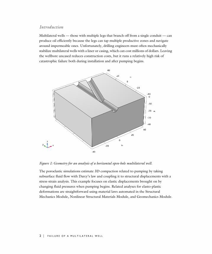
Multilateral wells — those with multiple legs that branch off from a single conduit — can produce oil efficiently because the legs can tap multiple productive zones and navigate around impermeable ones. Unfortunately, drilling engineers must often mechanically stabilize multilateral wells with a liner or casing, which can cost millions of dollars. Leaving the wellbore uncased reduces construction costs, but it runs a relatively high risk of catastrophic failure both during installation and after pumping begins.

Figure 1: Geometry for an analysis of a horizontal open-hole multilateral well.

The poroelastic simulations estimate 3D compaction related to pumping by taking subsurface fluid flow with Darcy’s law and coupling it to structural displacements with a stress-strain analysis. This example focuses on elastic displacements brought on by changing fluid pressures when pumping begins. Related analyses for elasto-plastic deformations are straightforward using material laws automated in the Structural Mechanics Module, Nonlinear Structural Materials Module, and Geomechanics Module.

2 | F A I L U R E O F A M U L T I L A T E R A L W E L L

Model Definition: Flow and Deformation Simulation

The modeled geometry (Figure 1) is the lower half of a branching junction, a segment from a larger well network. The junction lies roughly 25 feet from the start of the well. The entire well network extends much further, perhaps hundreds of feet. The well is 8.5 inches in diameter and sits in a cube 80 inches on each side. Pumps move fluid from the reservoir into the well. Fluid exits the geometry only through the well. The displacement at the reservoir edge is constrained. The walls of the well, however, deform freely. The goal is to solve for the change in fluid pressure, stress, strain, and displacement that the pumping causes rather than their absolute values.

F L U I D F L O W

To describe fluid flow, you insert the Darcy velocity into an equation of continuity

where κ is the permeability, μ is the dynamic viscosity, and p equals the pressure of the oil in the pores.

For the flow boundaries, you already know the change in fluid pressure from the well to the reservoir edge. The planar surface adjacent to the well (between the upper and lower blocks) is a symmetry boundary. Because the well is the only exit for the fluid, there is no flow to or from connecting well segments. In summary,

where n is the normal vector to the boundary.

S O L I D D E F O R M A T I O N

The system of equations that describes the quasi-static deformation is

∇ κμ---∇p–⋅ 0=

p pr= Ω reservoir∂

n κμ---∇p–

⋅ 0= Ω symmetry face∂

n κμ---∇p–

⋅ 0= Ω connecting segments∂

p pw= Ω well∂

∇– σ⋅ F=

3 | F A I L U R E O F A M U L T I L A T E R A L W E L L

where σ denotes the stress tensor, and F are external body forces. The stress tensor is augmented by the pressure load due to changes in pore pressure. In this model, the Biot-Willis coefficient is equal to one.

The stress-strain relationship for linear materials relates the stress tensor and the strain tensor ε through the elasticity matrix C, which for isotropic materials is a function of Young’s modulus, E, and Poisson’s ratio, ν.

In this geometrically linear example, the components of the strain tensor depend on the displacement vector u, which has directional components u, v, and w:

The tensors σ and ε are linearly related by Hooke’s law σ = C:ε .

For the boundary conditions, the example constrains movement at all external boundaries. The well opening is free to deform. In summary:

M O D E L D A T A

This model uses the coefficients and parameters listed in Table 1.

TABLE 1: MODEL DATA.

VARIABLE DESCRIPTION VALUE

ρf Fluid density 0.0361 lb/in3

κ Permeability 1·10-13 in2

μ Fluid dynamic viscosity 1·10-7 psi·s

E Young’s modulus 0.43·106 psi

ν Poisson’s ratio 0.16

ρs Solids density 0.0861 lb/in3

εx x∂∂u

=

εy y∂∂v

=

εz z∂∂w

=

εxy12---

y∂∂u

x∂∂v

+ =

εyz12---

z∂∂v

y∂∂w

+ =

εxz12---

z∂∂u

x∂∂w

+ =

u v w 0= = = Ω reservoir∂w 0= Ω symmetry face∂v 0= Ω connecting segments∂free Ω well∂

4 | F A I L U R E O F A M U L T I L A T E R A L W E L L

Results: Flow and Deformation Simulation

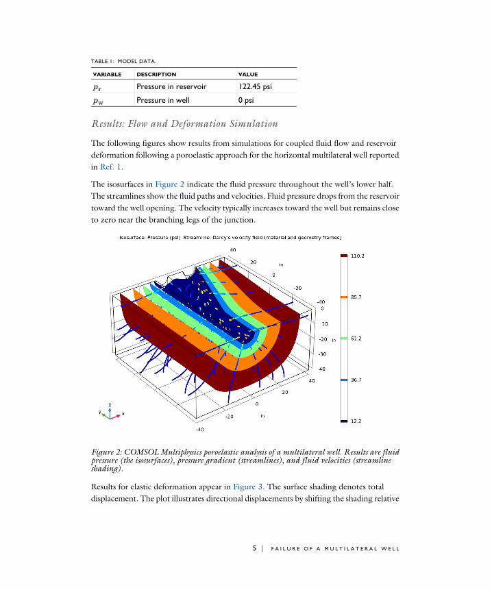
The following figures show results from simulations for coupled fluid flow and reservoir deformation following a poroelastic approach for the horizontal multilateral well reported in Ref. 1.

The isosurfaces in Figure 2 indicate the fluid pressure throughout the well’s lower half. The streamlines show the fluid paths and velocities. Fluid pressure drops from the reservoir toward the well opening. The velocity typically increases toward the well but remains close to zero near the branching legs of the junction.

Figure 2: COMSOL Multiphysics poroelastic analysis of a multilateral well. Results are fluid pressure (the isosurfaces), pressure gradient (streamlines), and fluid velocities (streamline shading).

Results for elastic deformation appear in Figure 3. The surface shading denotes total displacement. The plot illustrates directional displacements by shifting the shading relative

pr Pressure in reservoir 122.45 psi

pw Pressure in well 0 psi

TABLE 1: MODEL DATA.

VARIABLE DESCRIPTION VALUE

5 | F A I L U R E O F A M U L T I L A T E R A L W E L L

to an outline of the original geometry. For a clear view, the displacements are exaggerated. The uncased surface yields slightly because the deformed shading fills in the hollows of the well. The largest displacements occur just above the split in the well.

Figure 3: COMSOL Multiphysics estimates of displacement. Shading indicates the total displacement, and the geometry appears as lines. Even as the deformed shape shifts, those lines remain steady; the shaded image shows movement relative to the geometry outlines.

Failure Criterion

This model allows the evaluation of failures during postprocessing using results from the fluid-flow and solid-deformation simulations shown in the preceding figures. This discussion follows calculations that Ref. 1 uses to map calculations indicating where pumping could compact the reservoir enough (see Figure 3) that the well fails. Refer to Ref. 1 to estimate the critical rock strength required to successfully emplace the well, and also to learn more about calibration to data.

The 3D Coulomb failure criterion in Ref. 1 relates rock failure, the three principal stresses (σ1, σ2, and σ3), and the fluid pressures as follows:

6 | F A I L U R E O F A M U L T I L A T E R A L W E L L

(1)

Here So is the Coulomb cohesion and is the Coulomb friction angle. When properly calibrated, fail = 0 indicates the onset of rock failure; fail < 0 denotes catastrophic failure; and fail > 0 predicts stability. Because this model solves for the pressure change brought on by pumping as well as the stresses, strains, and displacements that the pressure change triggers, it calculates the expression just given using the change in pressure than its absolute value.

Results: Failure Criterion

The values for the fail function appear in Figure 4. When the fail values become increasingly negative, the potential for failure is higher. As expected, the fail function estimates show the greatest potential for failure just above the split in the well.

Figure 4: Values of the fail function calculated with results from a poroelastic model for the branching junction in an open-hole multilateral well. A negative value for the fail function denotes greater potential for failure.

fail σ3 p+( )= Q σ1 p+( ) N 1σ2 σ1–( )σ3 σ1–( )-----------------------+

+–

Q 1 φsin+1 φsin–----------------------, N 2 φcos

1 φsin–---------------------So==

φ

7 | F A I L U R E O F A M U L T I L A T E R A L W E L L

Conclusions

This example couples fluid flow and solid deformation for a poroelastic analysis using easy-to-use physics interfaces from COMSOL Multiphysics. The analysis provides estimates of the pressure change brought on by pumping as well as the stresses, strains, and displacements that the pressure drop triggers. Combining the simulation results with a 3D Coulomb failure expression, maps vulnerability to mechanical failure from the pumping. The data and geometry for this model come from petroleum industry analyses by TerraTek (Ref. 1), which in turn use failure criteria to map the potential for failure during emplacement of the well in addition to the potential for failure when the well is pumped.

Reference

1. R. Suarez-Rivera, B.J. Begnaud, and W.J. Martin, “Numerical Analysis of Open-hole Multilateral Completions Minimizes the Risk of Costly Junction Failures,” Rio Oil & Gas Expo and Conference (IBP096_04), 2004.

Application Library path: Subsurface_Flow_Module/Flow_and_Solid_Deformation/multilateral_well

Modeling Instructions

From the File menu, choose New.

N E W

In the New window, click Model Wizard.

M O D E L W I Z A R D

1 In the Model Wizard window, click 3D.

2 In the Select Physics tree, select Structural Mechanics>Poroelasticity>Poroelasticity, Solid.

3 Click Add.

4 Click Study.

5 In the Select Study tree, select General Studies>Stationary.

6 Click Done.

8 | F A I L U R E O F A M U L T I L A T E R A L W E L L

G E O M E T R Y 1

1 In the Model Builder window, under Component 1 (comp1) click Geometry 1.

2 In the Settings window for Geometry, locate the Units section.

3 From the Length unit list, choose in.

Import 1 (imp1)1 In the Home toolbar, click Import.

2 In the Settings window for Import, locate the Import section.

3 Click Browse.

4 Browse to the model’s Application Libraries folder and double-click the file multilateral_well.mphbin.

5 Click Import.

G L O B A L D E F I N I T I O N S

Parameters 11 In the Model Builder window, under Global Definitions click Parameters 1.

2 In the Settings window for Parameters, locate the Parameters section.

3 In the table, enter the following settings:

D E F I N I T I O N S

Variables 11 In the Home toolbar, click Variables and choose Local Variables.

2 In the Settings window for Variables, locate the Variables section.

Name Expression Value Description

p_r 122.45[psi] 8.4426E5 Pa Pressure in reservoir

p_w 0[psi] 0 Pa Pressure in well

So 850[psi] 5.8605E6 Pa Coulomb cohesion

phi 31[deg] 0.54105 rad Friction angle

C1 14.7 14.7 Calibration constant 1

C2 40 40 Calibration constant 2

suppX 0 0 Well support, x-component

suppY 0 0 Well support, y-component

suppZ 0 0 Well support, z-component

9 | F A I L U R E O F A M U L T I L A T E R A L W E L L

3 In the table, enter the following settings:

Here, solid.sp1, solid.sp2, and solid.sp3 are the principal stresses. Note that the expression fail defined in Equation 1 has the dimension of stress. By appending the operator [1/psi] to the dimensionful expression enclosed within parentheses you extract its value in psi, which is what Ref. 1 uses. This way, you can analyze the risk for rock failure using the same criterion independently of your choice of base unit system.

M A T E R I A L S

Create two materials: one for the porous matrix, and one for the fluid.

Porous Matrix1 In the Model Builder window, under Component 1 (comp1) right-click Materials and

choose Blank Material.

2 In the Settings window for Material, type Porous Matrix in the Label text field.

Fluid1 Right-click Materials and choose Blank Material.

2 In the Settings window for Material, type Fluid in the Label text field.

The fluid material has no selection. Select it manually in the Poroelastic Storage model.

D A R C Y ’ S L A W ( D L )

Poroelastic Storage 11 In the Model Builder window, under Component 1 (comp1)>Darcy’s Law (dl) click

Poroelastic Storage 1.

2 In the Settings window for Poroelastic Storage, locate the Fluid Properties section.

3 From the Fluid material list, choose Fluid (mat2).

Name Expression Unit Description

N 2*So*cos(phi)/(1-sin(phi))

Pa Fail parameter 1

Q (1+sin(phi))/(1-sin(phi))

Fail parameter 2

fail (((solid.sp3+C1*(p_r-p))-Q*(solid.sp1+C1*(p_r-p))+N*(1+(solid.sp2-solid.sp1)/(solid.sp3-solid.sp1)))/C2)[1/psi]

Fail expression

10 | F A I L U R E O F A M U L T I L A T E R A L W E L L

M A T E R I A L S

Porous Matrix (mat1)1 In the Model Builder window, under Component 1 (comp1)>Materials click

Porous Matrix (mat1).

2 In the Settings window for Material, locate the Material Contents section.

3 In the table, enter the following settings:

Fluid (mat2)1 In the Model Builder window, click Fluid (mat2).

2 In the Settings window for Material, locate the Material Contents section.

3 In the table, enter the following settings:

S O L I D M E C H A N I C S ( S O L I D )

In the Model Builder window, under Component 1 (comp1) click Solid Mechanics (solid).

Fixed Constraint 11 In the Physics toolbar, click Boundaries and choose Fixed Constraint.

2 Select Boundaries 1, 3, and 13 only.

Property Variable Value Unit Property group

Young’s modulus E 4.3e5[psi] Pa Basic

Poisson’s ratio nu 0.16 1 Basic

Density rho 0.0861[lb/in^3]

kg/m³ Basic

Porosity epsilon 0.3 1 Basic

Permeability kappa_iso ; kappaii = kappa_iso, kappaij = 0

1e-13[in^2] m² Basic

Biot-Willis coefficient

alphaB 1 1 Poroelastic material

Property Variable Value Unit Property group

Compressibility of fluid

chif 4e-10 1/Pa Basic

Density rho 0.0361[lb/in^3] kg/m³ Basic

Dynamic viscosity mu 1e-7[psi*s] Pa·s Basic

11 | F A I L U R E O F A M U L T I L A T E R A L W E L L

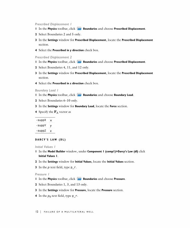
Prescribed Displacement 11 In the Physics toolbar, click Boundaries and choose Prescribed Displacement.

2 Select Boundaries 2 and 5 only.

3 In the Settings window for Prescribed Displacement, locate the Prescribed Displacement section.

4 Select the Prescribed in y direction check box.

Prescribed Displacement 21 In the Physics toolbar, click Boundaries and choose Prescribed Displacement.

2 Select Boundaries 4, 11, and 12 only.

3 In the Settings window for Prescribed Displacement, locate the Prescribed Displacement section.

4 Select the Prescribed in z direction check box.

Boundary Load 11 In the Physics toolbar, click Boundaries and choose Boundary Load.

2 Select Boundaries 6–10 only.

3 In the Settings window for Boundary Load, locate the Force section.

4 Specify the FA vector as

D A R C Y ’ S L A W ( D L )

Initial Values 11 In the Model Builder window, under Component 1 (comp1)>Darcy’s Law (dl) click

Initial Values 1.

2 In the Settings window for Initial Values, locate the Initial Values section.

3 In the p text field, type p_r.

Pressure 11 In the Physics toolbar, click Boundaries and choose Pressure.

2 Select Boundaries 1, 3, and 13 only.

3 In the Settings window for Pressure, locate the Pressure section.

4 In the p0 text field, type p_r.

-suppX x

-suppY y

-suppZ z

12 | F A I L U R E O F A M U L T I L A T E R A L W E L L

Pressure 21 In the Physics toolbar, click Boundaries and choose Pressure.

2 Select Boundaries 6–10 only.

3 In the Settings window for Pressure, locate the Pressure section.

4 In the p0 text field, type p_w.

S T U D Y 1

1 In the Model Builder window, click Study 1.

2 In the Settings window for Study, locate the Study Settings section.

3 Clear the Generate default plots check box.

4 In the Home toolbar, click Compute.

R E S U L T S

Create a plot which shows the displacement as in Figure 3.

Displacement1 In the Home toolbar, click Add Plot Group and choose 3D Plot Group.

2 In the Settings window for 3D Plot Group, type Displacement in the Label text field.

Surface 1Right-click Displacement and choose Surface.

Deformation 11 In the Model Builder window, right-click Surface 1 and choose Deformation.

2 In the Settings window for Deformation, locate the Scale section.

3 Select the Scale factor check box.

4 In the associated text field, type 1000.

5 In the Displacement toolbar, click Plot.

Next, create a plot that visualizes the pressure and velocity fields like in Figure 2.

Fluid Pressure and Velocities1 In the Home toolbar, click Add Plot Group and choose 3D Plot Group.

2 In the Settings window for 3D Plot Group, type Fluid Pressure and Velocities in the Label text field.

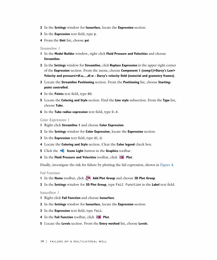
Isosurface 11 Right-click Fluid Pressure and Velocities and choose Isosurface.

13 | F A I L U R E O F A M U L T I L A T E R A L W E L L

2 In the Settings window for Isosurface, locate the Expression section.

3 In the Expression text field, type p.

4 From the Unit list, choose psi.

Streamline 11 In the Model Builder window, right-click Fluid Pressure and Velocities and choose

Streamline.

2 In the Settings window for Streamline, click Replace Expression in the upper-right corner of the Expression section. From the menu, choose Component 1 (comp1)>Darcy’s Law>

Velocity and pressure>dl.u,...,dl.w - Darcy’s velocity field (material and geometry frames).

3 Locate the Streamline Positioning section. From the Positioning list, choose Starting-

point controlled.

4 In the Points text field, type 60.

5 Locate the Coloring and Style section. Find the Line style subsection. From the Type list, choose Tube.

6 In the Tube radius expression text field, type 0.4.

Color Expression 11 Right-click Streamline 1 and choose Color Expression.

2 In the Settings window for Color Expression, locate the Expression section.

3 In the Expression text field, type dl.U.

4 Locate the Coloring and Style section. Clear the Color legend check box.

5 Click the Scene Light button in the Graphics toolbar.

6 In the Fluid Pressure and Velocities toolbar, click Plot.

Finally, investigate the risk for failure by plotting the fail expression, shown in Figure 4.

Fail Function1 In the Home toolbar, click Add Plot Group and choose 3D Plot Group.

2 In the Settings window for 3D Plot Group, type Fail Function in the Label text field.

Isosurface 11 Right-click Fail Function and choose Isosurface.

2 In the Settings window for Isosurface, locate the Expression section.

3 In the Expression text field, type fail.

4 In the Fail Function toolbar, click Plot.

5 Locate the Levels section. From the Entry method list, choose Levels.

14 | F A I L U R E O F A M U L T I L A T E R A L W E L L

6 Click Range.

7 In the Range dialog box, type -20 in the Start text field.

8 In the Stop text field, type 20.

9 In the Step text field, type 10.

10 Click Replace.

11 In the Settings window for Isosurface, locate the Coloring and Style section.

12 From the Color table list, choose WaveLight.

13 In the Fail Function toolbar, click Plot.

15 | F A I L U R E O F A M U L T I L A T E R A L W E L L

16 | F A I L U R E O F A M U L T I L A T E R A L W E L L