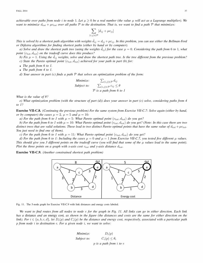
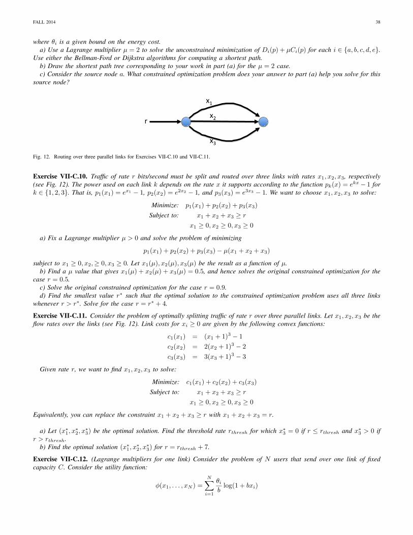
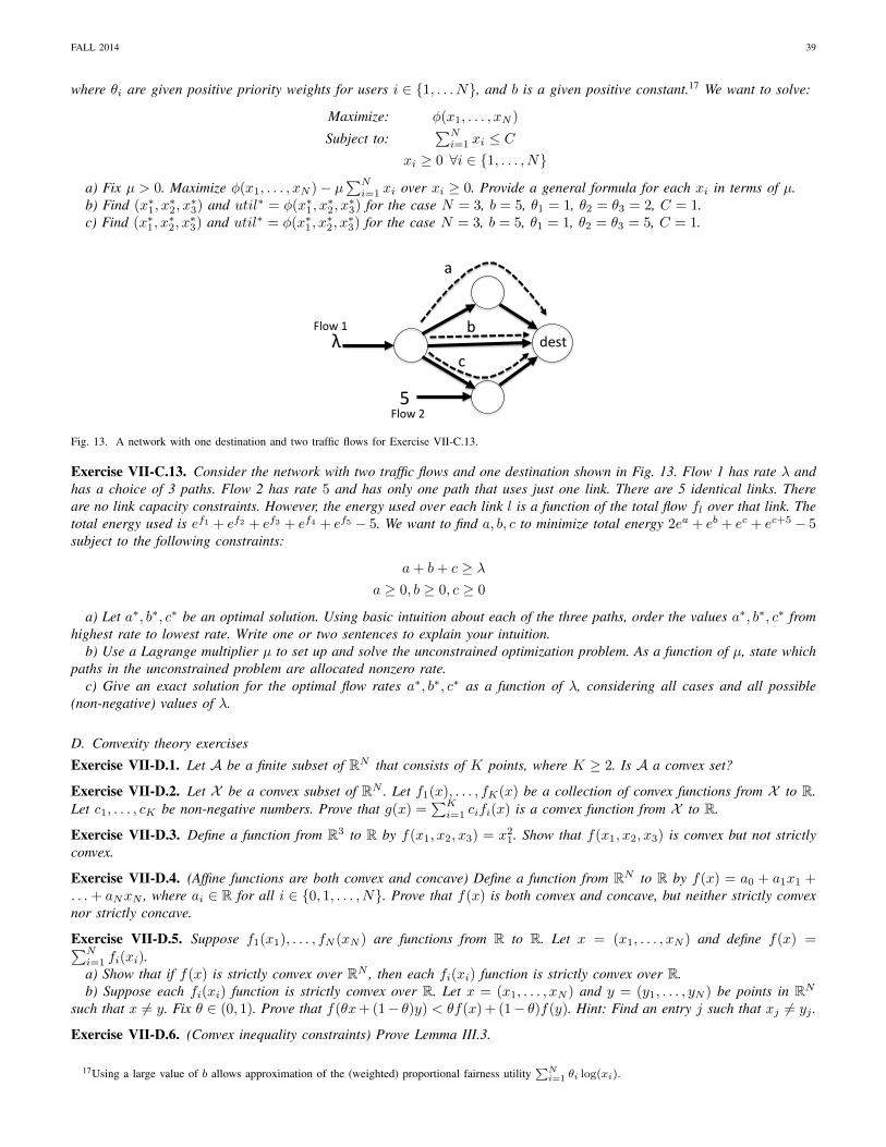
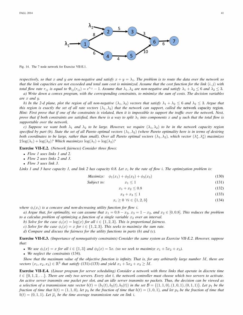
FALL 2014 1

Network Optimization: Notes and ExercisesMichael J. Neely

University of Southern Californiahttp://www-bcf.usc.edu/∼mjneely

Abstract

These notes provide a tutorial treatment of topics of Pareto optimality, Lagrange multipliers, and computational algorithmsfor multiobjective optimization, with emphasis on applications to data networks. Problems with two objectives are consideredfirst, called bicriteria optimization problems (treated in Sections I and II). The main concepts of bicriteria optimization naturallyextend to problems with more than two objectives, called multicriteria optimization problems. Multicriteria problems can be morecomplex than bicriteria problems, and often cannot be solved without the aid of a computer. Efficient computational methods existfor problems that have a convex structure. Convexity is formally defined in Section III. Section IV describes a general class ofmulticriteria problems with a convex structure, called convex programs. A drift-plus-penalty algorithm is developed in Section Vas a computational procedure for solving convex programs. The drift-plus-penalty algorithm extends as an online control techniquefor optimizing time averages of system objectives, even when the underlying system does not have a convex structure. SectionVI focuses on application of drift-plus-penalty theory to multi-hop networks, including problems of network utility maximizationand power-aware routing. Exercises are provided to reinforce the theory and the applications.

HOW TO REFERENCE THESE NOTES

Sections I-IV present well known material on optimization (see also [1][2]). Sections V-VI present more recent material ondrift-plus-penalty theory for convex programs and data networks. Readers who want to cite the drift-plus-penalty material inthese notes should cite the published works [3] and [4].

I. BICRITERIA OPTIMIZATION

Consider a system that has a collection M of different operating modes, where M is an abstract (possibly infinite) set thatcontains at least one element. Each operating mode m ∈M determines a two-dimensional vector (x(m), y(m)), where x(m)and y(m) represent distinct system objectives of interest. Suppose it is desirable to keep both objectives x(m) and y(m) assmall as possible. We want to find a mode m ∈M that “minimizes both” x(m) and y(m). Of course, it may not be possibleto simultaneously minimize both objectives. This tension motivates the study of bicriteria optimization.

Example I.1. Consider the problem of finding the best route to use for sending a single message over a network. Let Mrepresent the set of all possible routes. Suppose each link (i, j) has a link distance dij and a link energy expenditure eij . Foreach route m ∈M, let x(m) be the total distance of the route, and let y(m) be the total energy used. It is desirable to keepboth objectives x(m) and y(m) small.

Example I.2. Consider the problem of transmitting over a single wireless link. Let p be a variable that represents the amountof power used, and suppose this variable must be chosen over an interval [0, pmax] for some positive maximum power levelpmax. The power used determines the transmission rate µ(p) = log(1 +p). The goal is to operate the system while minimizingpower and maximizing transmission rate. Define set M as the interval [0, pmax]. For each p ∈ M, define x(p) = p as thepower used and y(p) = −µ(p) as −1 times the transmission rate achieved (so that minimizing y(p) is the same as maximizingµ(p)). We want to choose p ∈M to keep both objectives x(p) and y(p) small.

Example I.3. Consider a wireless device that transmits to three different users over orthogonal links. The device must choosea power vector (p1, p2, p3) ∈ R3 that satisfies the following constraints:

p1 + p2 + p3 ≤ pmax (1)pi > 0 ∀i ∈ 1, 2, 3 (2)

where pmax is a positive real number that constrains the sum power usage. For each i ∈ 1, 2, 3, let µi(pi) = log(1+γipi) bethe transmission rate achieved over link i as a function of the power variable pi, where γi is some known attenuation coefficientfor link i. Define M as the set of all (p1, p2, p3) ∈ R3 that satisfy the constraints (1)-(2). Define x(p1, p2, p3) = p1 + p2 + p3as the sum power used. Define y(p1, p2, p3) = −[µ1(p1) + µ2(p2) + µ3(p3)] as −1 times the sum rate over all three links.The goal is to choose (p1, p2, p3) ∈M to keep both x(p1, p2, p3) and y(p1, p2, p3) small.

Example I.4. Consider the same 3-link wireless system as Example I.3. However, suppose we do not care about powerexpenditure. Rather, we care about:• Maximizing the sum rate µ1(p1) + µ2(p2) + µ3(p3).

FALL 2014 2

• Maximizing the proportionally fair utility metric log(µ1(p1))+log(µ2(p2))+log(µ3(p3)). This is a commonly used notionof fairness for rate allocation over multiple users.1

Again letM be the set of all vectors (p1, p2, p3) ∈ R3 that satisfy (1)-(2). Define x(p1, p2, p3) = −[µ1(p1)+µ2(p2)+µ3(p3)]as −1 times the sum rate, and define y(p1, p2, p3) = −[log(µ1(p1))+log(µ2(p2))+log(µ3(p3))] as −1 times the proportionallyfair utility metric. The goal is to choose (p1, p2, p3) ∈M to minimize both x(p1, p2, p3) and y(p1, p2, p3).

Examples I.2-I.4 illustrate how a bicriteria optimization problem that seeks to maximize one objective while minimizinganother, or that seeks to maximize both objectives, can be transformed into a bicriteria minimization problem by multiplyingthe appropriate objectives by −1. Hence, without loss of generality, it suffices to assume the system controller wants bothcomponents of the vector of objectives (x, y) to be small.

A. Pareto optimality

Define A as the set of all (x, y) vectors in R2 that are achievable via system modes m ∈M:

A = (x(m), y(m)) ∈ R2|m ∈M

Every (x, y) pair in A is a feasible operating point. Once the set A is known, system optimality can be understood in termsof selecting a desirable 2-dimensional vector (x, y) in the set A. With this approach, the study of optimality does not requireknowledge of the physical tasks the system must perform for each mode of operation in M. This is useful because it allowsmany different types of problems to be treated with a common mathematical framework.

The set A can have an arbitrary structure. It can be finite, infinite, closed, open, neither closed nor open, and so on. Assumethe system controller wants to find an operating point (x, y) ∈ A for which both x and y are small.

Definition I.1. A vector (x, y) ∈ A dominates (or is “preferred over”) another vector (w, z) ∈ A, written (x, y) ≺ (w, z), ifthe following two inequalities hold• x ≤ w• y ≤ z

and if at least one of the inequalities is strict (so that either x < w or y < z).

Definition I.2. A vector (x∗, y∗) ∈ A is Pareto optimal if there is no vector (x, y) ∈ A that satisfies (x, y) ≺ (x∗, y∗).

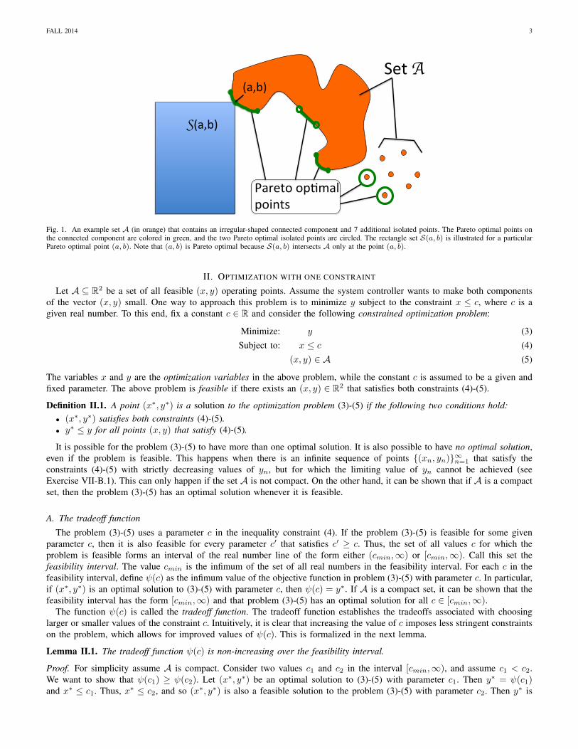
A set can have many Pareto optimal points. An example set A and its Pareto optimal points are shown in Fig. 1. For eachvector (a, b) ∈ R2, define S(a, b) as the set of all points (x, y) that satisfy x ≤ a and y ≤ b:

S(a, b) = (x, y) ∈ R2|x ≤ a, y ≤ b

Pictorially, the set S(a, b) is an infinite square in the 2-dimesional plane with upper-right vertex at (a, b) (see Fig. 1). If (a, b)is a point in A, any other vector in A that dominates (a, b) must lie in the set S(a, b). If there are no points in A ∩ S(a, b)other than (a, b) itself, then (a, b) is Pareto optimal.

B. Degenerate cases and the compact assumption

In some cases the set A will have no Pareto optimal points. For example, suppose A is the entire set R2. If we chooseany point (x, y) ∈ R2, there is always another point (x − 1, y) ∈ R2 that dominates. Further, it can be shown that if A isan open subset of R2, then it has no Pareto optimal points (see Exercise VII-A.5). To avoid these degenerate situations, it isoften useful to impose the further condition that the set A is both closed and bounded. A closed and bounded subset of RNis called a compact set. If A is a finite set then it is necessarily compact.

It can be shown that if A is a nonempty compact set, then:1) It has Pareto optimal points.2) For every point (x, y) ∈ A that is not Pareto optimal, there is a Pareto optimal point that dominates (x, y).

Therefore, when A is compact, it suffices to restrict attention to choosing an operating point (x, y) that is Pareto optimal.

1See [5] for a development of proportionally fair utility and its relation to the log(µ) function. The constraints (2) avoid the singularity of the log(µ)function at 0, so that log(µ1(p1)) + log(µ2(p2)) + log(µ3(p3)) is indeed a real number whenever (p1, p2, p3) satisfies (1)-(2). An alternative is to useconstraints pi ≥ 0 (which allow zero power in some channels), but to modify the utility function from log(µ) to (1/b) log(1 + bµ) for some constant b > 0.

FALL 2014 3

Set$A

Pareto$op*mal$$points$

(a,b)$

S(a,b)$

Fig. 1. An example set A (in orange) that contains an irregular-shaped connected component and 7 additional isolated points. The Pareto optimal points onthe connected component are colored in green, and the two Pareto optimal isolated points are circled. The rectangle set S(a, b) is illustrated for a particularPareto optimal point (a, b). Note that (a, b) is Pareto optimal because S(a, b) intersects A only at the point (a, b).

II. OPTIMIZATION WITH ONE CONSTRAINT

Let A ⊆ R2 be a set of all feasible (x, y) operating points. Assume the system controller wants to make both componentsof the vector (x, y) small. One way to approach this problem is to minimize y subject to the constraint x ≤ c, where c is agiven real number. To this end, fix a constant c ∈ R and consider the following constrained optimization problem:

Minimize: y (3)Subject to: x ≤ c (4)

(x, y) ∈ A (5)

The variables x and y are the optimization variables in the above problem, while the constant c is assumed to be a given andfixed parameter. The above problem is feasible if there exists an (x, y) ∈ R2 that satisfies both constraints (4)-(5).

Definition II.1. A point (x∗, y∗) is a solution to the optimization problem (3)-(5) if the following two conditions hold:• (x∗, y∗) satisfies both constraints (4)-(5).• y∗ ≤ y for all points (x, y) that satisfy (4)-(5).

It is possible for the problem (3)-(5) to have more than one optimal solution. It is also possible to have no optimal solution,even if the problem is feasible. This happens when there is an infinite sequence of points (xn, yn)∞n=1 that satisfy theconstraints (4)-(5) with strictly decreasing values of yn, but for which the limiting value of yn cannot be achieved (seeExercise VII-B.1). This can only happen if the set A is not compact. On the other hand, it can be shown that if A is a compactset, then the problem (3)-(5) has an optimal solution whenever it is feasible.

A. The tradeoff function

The problem (3)-(5) uses a parameter c in the inequality constraint (4). If the problem (3)-(5) is feasible for some givenparameter c, then it is also feasible for every parameter c′ that satisfies c′ ≥ c. Thus, the set of all values c for which theproblem is feasible forms an interval of the real number line of the form either (cmin,∞) or [cmin,∞). Call this set thefeasibility interval. The value cmin is the infimum of the set of all real numbers in the feasibility interval. For each c in thefeasibility interval, define ψ(c) as the infimum value of the objective function in problem (3)-(5) with parameter c. In particular,if (x∗, y∗) is an optimal solution to (3)-(5) with parameter c, then ψ(c) = y∗. If A is a compact set, it can be shown that thefeasibility interval has the form [cmin,∞) and that problem (3)-(5) has an optimal solution for all c ∈ [cmin,∞).

The function ψ(c) is called the tradeoff function. The tradeoff function establishes the tradeoffs associated with choosinglarger or smaller values of the constraint c. Intuitively, it is clear that increasing the value of c imposes less stringent constraintson the problem, which allows for improved values of ψ(c). This is formalized in the next lemma.

Lemma II.1. The tradeoff function ψ(c) is non-increasing over the feasibility interval.

Proof. For simplicity assume A is compact. Consider two values c1 and c2 in the interval [cmin,∞), and assume c1 < c2.We want to show that ψ(c1) ≥ ψ(c2). Let (x∗, y∗) be an optimal solution to (3)-(5) with parameter c1. Then y∗ = ψ(c1)and x∗ ≤ c1. Thus, x∗ ≤ c2, and so (x∗, y∗) is also a feasible solution to the problem (3)-(5) with parameter c2. Then y∗ is

FALL 2014 4

c"

ψ(c)"

cmin"c1" c2" c3"

Fig. 2. The set A from Fig. 1 with its (non-increasing) tradeoff function ψ(c) drawn in green. Note that ψ(c) is discontinuous at points c1, c2, c3.

greater than or equal to the optimal objective function value for the problem (3)-(5) with parameter c2, which is ψ(c2). Thatis, ψ(c1) = y∗ ≥ ψ(c2).

Note that the tradeoff function ψ(c) is not necessarily continuous (see Fig. 2). It can be shown that it is continuous whenthe set A is compact and has a convexity property.2 Convexity is defined in Section III.

The tradeoff curve is defined as the set of all points (c, ψ(c)) for c in the feasibility interval. Exercise VII-A.8 shows thatevery Pareto optimal point (x(p), y(p)) of A is a point on the tradeoff curve, so that ψ(x(p)) = y(p).

B. Lagrange multipliers for optimization over (x, y) ∈ AThe constrained optimization problem (3)-(5) may be difficult to solve because of the inequality constraint (4). Consider the

following related problem, defined in terms of a real number µ ≥ 0:

Minimize: y + µx (6)Subject to: (x, y) ∈ A (7)

The problem (6)-(7) is called the unconstrained optimization problem because it has no inequality constraint. Of course, itstill has the set constraint (7). The constant µ is called a Lagrange multiplier. It acts as a weight that determines the relativeimportance of making the x component small when minimizing the objective function (6). Note that if (x∗, y∗) is a solutionto the unconstrained optimization problem (6)-(7) for a particular value µ, then:

y∗ + µx∗ ≤ y + µx for all (x, y) ∈ A (8)

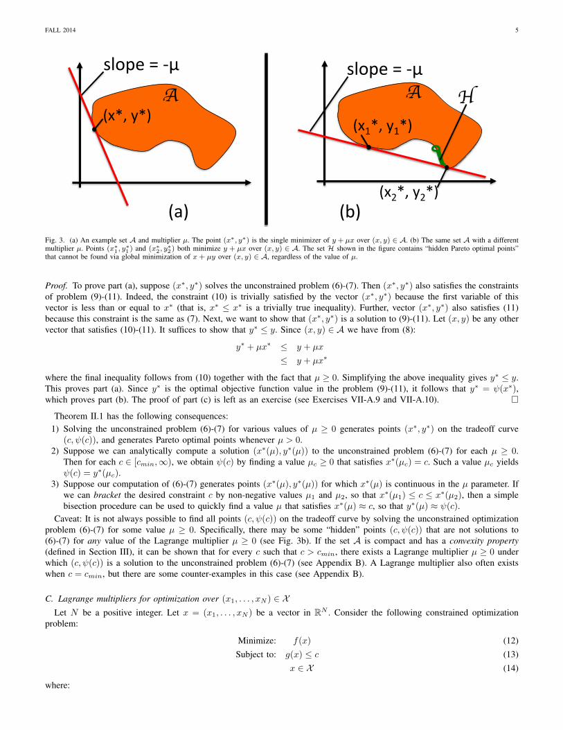
In particular, all points of the set A are on or above the line consisting of points (x, y) that satisfy y + µx = y∗ + µx∗. Thisline has slope −µ and touches the set A at the point (x∗, y∗) (see Fig. 3).

Theorem II.1. If (x∗, y∗) solves the unconstrained problem (6)-(7), then:a) If µ ≥ 0, then (x∗, y∗) solves the following optimization problem (where (x, y) are the optimization variables and x∗ is

treated as a given parameter):

Minimize: y (9)Subject to: x ≤ x∗ (10)

(x, y) ∈ A (11)

b) If µ ≥ 0, then (x∗, y∗) is a point on the tradeoff curve (c, ψ(c)). Specifically, ψ(x∗) = y∗.c) If µ > 0, then (x∗, y∗) is Pareto optimal in A.

2In particular, ψ(c) is both continuous and convex over c ∈ [cmin,∞) whenever A is compact and convex. Definitions of convex set and convex functionare provided in Section III.

FALL 2014 5

(x1*,&y1*)&

slope&=&/μ&

(x2*,&y2*)&

(x*,&y*)&

slope&=&/μ&

(b)&&(a)&&

H A A

Fig. 3. (a) An example set A and multiplier µ. The point (x∗, y∗) is the single minimizer of y + µx over (x, y) ∈ A. (b) The same set A with a differentmultiplier µ. Points (x∗1, y

∗1) and (x∗2, y

∗2) both minimize y + µx over (x, y) ∈ A. The set H shown in the figure contains “hidden Pareto optimal points”

that cannot be found via global minimization of x+ µy over (x, y) ∈ A, regardless of the value of µ.

Proof. To prove part (a), suppose (x∗, y∗) solves the unconstrained problem (6)-(7). Then (x∗, y∗) also satisfies the constraintsof problem (9)-(11). Indeed, the constraint (10) is trivially satisfied by the vector (x∗, y∗) because the first variable of thisvector is less than or equal to x∗ (that is, x∗ ≤ x∗ is a trivially true inequality). Further, vector (x∗, y∗) also satisfies (11)because this constraint is the same as (7). Next, we want to show that (x∗, y∗) is a solution to (9)-(11). Let (x, y) be any othervector that satisfies (10)-(11). It suffices to show that y∗ ≤ y. Since (x, y) ∈ A we have from (8):

y∗ + µx∗ ≤ y + µx

≤ y + µx∗

where the final inequality follows from (10) together with the fact that µ ≥ 0. Simplifying the above inequality gives y∗ ≤ y.This proves part (a). Since y∗ is the optimal objective function value in the problem (9)-(11), it follows that y∗ = ψ(x∗),which proves part (b). The proof of part (c) is left as an exercise (see Exercises VII-A.9 and VII-A.10).

Theorem II.1 has the following consequences:1) Solving the unconstrained problem (6)-(7) for various values of µ ≥ 0 generates points (x∗, y∗) on the tradeoff curve

(c, ψ(c)), and generates Pareto optimal points whenever µ > 0.2) Suppose we can analytically compute a solution (x∗(µ), y∗(µ)) to the unconstrained problem (6)-(7) for each µ ≥ 0.

Then for each c ∈ [cmin,∞), we obtain ψ(c) by finding a value µc ≥ 0 that satisfies x∗(µc) = c. Such a value µc yieldsψ(c) = y∗(µc).

3) Suppose our computation of (6)-(7) generates points (x∗(µ), y∗(µ)) for which x∗(µ) is continuous in the µ parameter. Ifwe can bracket the desired constraint c by non-negative values µ1 and µ2, so that x∗(µ1) ≤ c ≤ x∗(µ2), then a simplebisection procedure can be used to quickly find a value µ that satisfies x∗(µ) ≈ c, so that y∗(µ) ≈ ψ(c).

Caveat: It is not always possible to find all points (c, ψ(c)) on the tradeoff curve by solving the unconstrained optimizationproblem (6)-(7) for some value µ ≥ 0. Specifically, there may be some “hidden” points (c, ψ(c)) that are not solutions to(6)-(7) for any value of the Lagrange multiplier µ ≥ 0 (see Fig. 3b). If the set A is compact and has a convexity property(defined in Section III), it can be shown that for every c such that c > cmin, there exists a Lagrange multiplier µ ≥ 0 underwhich (c, ψ(c)) is a solution to the unconstrained problem (6)-(7) (see Appendix B). A Lagrange multiplier also often existswhen c = cmin, but there are some counter-examples in this case (see Appendix B).

C. Lagrange multipliers for optimization over (x1, . . . , xN ) ∈ XLet N be a positive integer. Let x = (x1, . . . , xN ) be a vector in RN . Consider the following constrained optimization

problem:

Minimize: f(x) (12)Subject to: g(x) ≤ c (13)

x ∈ X (14)

where:

FALL 2014 6

• X is a general subset of RN .• f(x) and g(x) are real-valued functions defined over X .• c is a given real number.The tradeoff function ψ(c) associated with problem (12)-(14) is defined as the infimum objective function value over all x ∈ X

that satisfy the constraint g(x) ≤ c. In particular, if x∗ is a solution to problem (12)-(14) with parameter c, then ψ(c) = f(x∗).The problem (12)-(14) is similar to the problem (3)-(5). In fact, it can be viewed as a special case of the problem (3)-(5) ifwe define A as the set of all vectors (g, f) ∈ R2 such that (g, f) = (g(x), f(x)) for some x = (x1, . . . , xN ) ∈ X . Thus, aLagrange multiplier approach is also effective for the problem (12)-(14). Fix a Lagrange multiplier µ ≥ 0 and consider theunconstrained problem:

Minimize: f(x) + µg(x) (15)Subject to: x ∈ X (16)

As before, choosing a large value of µ for the problem (15)-(16) places more emphasis on keeping g(x) small. If x∗ =(x∗1, . . . , x

∗N ) is an optimal solution to the unconstrained problem (15)-(16), then

f(x∗) + µg(x∗) ≤ f(x) + µg(x) for all x ∈ X (17)

Theorem II.2. Suppose µ ≥ 0. If x∗ = (x∗1, . . . , x∗N ) is an optimal solution to the unconstrained problem (15)-(16), then it is

also an optimal solution to the following problem:

Minimize: f(x) (18)Subject to: g(x) ≤ g(x∗) (19)

x ∈ X (20)

Proof. Suppose x∗ = (x∗1, . . . , x∗N ) solves (15)-(16). Then this vector also satisfies all constraints of problem (18)-(20). Now

suppose x = (x1, . . . , xN ) is another vector that satisfies the constraints (19)-(20). We want to show that f(x∗) ≤ f(x). Sincex ∈ X , we have from (17):

f(x∗) + µg(x∗) ≤ f(x) + µg(x)

≤ f(x) + µg(x∗)

where the final inequality holds because µ ≥ 0 and because x satisfies (19). Canceling common terms in the above inequalityproves f(x∗) ≤ f(x).

The above theorem extends easily to the case of multiple constraints (see Exercise VII-B.2).

Example II.1. Minimize the function∑Ni=1 aixi subject to

∑Ni=1 bix

2i ≤ 4 and (x1, . . . , xN ) ∈ RN , where (a1, . . . , aN ) and

(b1, . . . , bN ) are given real numbers such that bi > 0 for all i.Solution: Fix µ ≥ 0. We minimize

∑Ni=1 aixi + µ

∑Ni=1 bix

2i over (x1, . . . , xN ) ∈ RN . This is a separable minimization of

aixi + µbix2i for each variable xi ∈ R. When µ > 0, the result is xi = −ai/(2µbi) for i ∈ 1, . . . , N. Choosing µ to satisfy

the constraint with equality gives 4 =∑Nj=1 bjx

2j =

∑Nj=1 bj(−aj/(2µbj))2. Thus:

µ∗ =1

4

√√√√ N∑j=1

a2j/bj

and x∗i = −ai/(2µ∗bi) for all i ∈ 1, . . . , N. This is optimal by Theorem II.2.

D. Critical points for unconstrained optimization

If a real-valued function f(x) of a multi-dimensional vector x = (x1, . . . , xN ) is differentiable at a point x = (x1, . . . , xN ) ∈RN , its gradient is the vector of partial derivatives:

∇f(x) =

[∂f(x)

∂x1,∂f(x)

∂x2, . . . ,

∂f(x)

∂xN

]The problem (15)-(16) seeks to find a global minimum of the function f(x) + µg(x) over all vectors x = (x1, . . . , xN ) in

the set X . Recall from basic calculus that, if a global minimum exists, it must occur at a critical point. Specifically, a pointx∗ = (x∗1, . . . , x

∗N ) is a critical point for this problem if x∗ ∈ X and if x∗ satisfies at least one of the following three criteria:3

3A boundary point of a set X ⊆ RN is a point x ∈ RN that is arbitrarily close to points in X and also arbitrarily close to points not in X . The set RNhas no boundary points. A set is closed if and only if it contains all of its boundary points. A set is open if and only if it contains none of its boundarypoints. A point in X is an interior point if and only if it is not a boundary point.

FALL 2014 7

• x∗ is on the boundary of X .• ∇f(x∗) + µ∇g(x∗) does not exist as a finite vector in RN .• ∇f(x∗) + µ∇g(x∗) = 0 (where the “0” on the right-hand-side represents the all-zero vector).

The condition ∇f(x∗) + µ∇g(x∗) = 0 is called the stationary equation. While this condition arises in the search for aglobal minimum of f(x) + µg(x), it can also find local minima or local maxima. It turns out that such critical points areoften important. In particular, for some non-convex problems, a search for solutions that solve the stationary equation canreveal points (g(x), f(x)) that lie on the tradeoff curve (c, ψ(c)), even when it is impossible to find such points via a globalminimization (see Appendix A for a development of this idea).

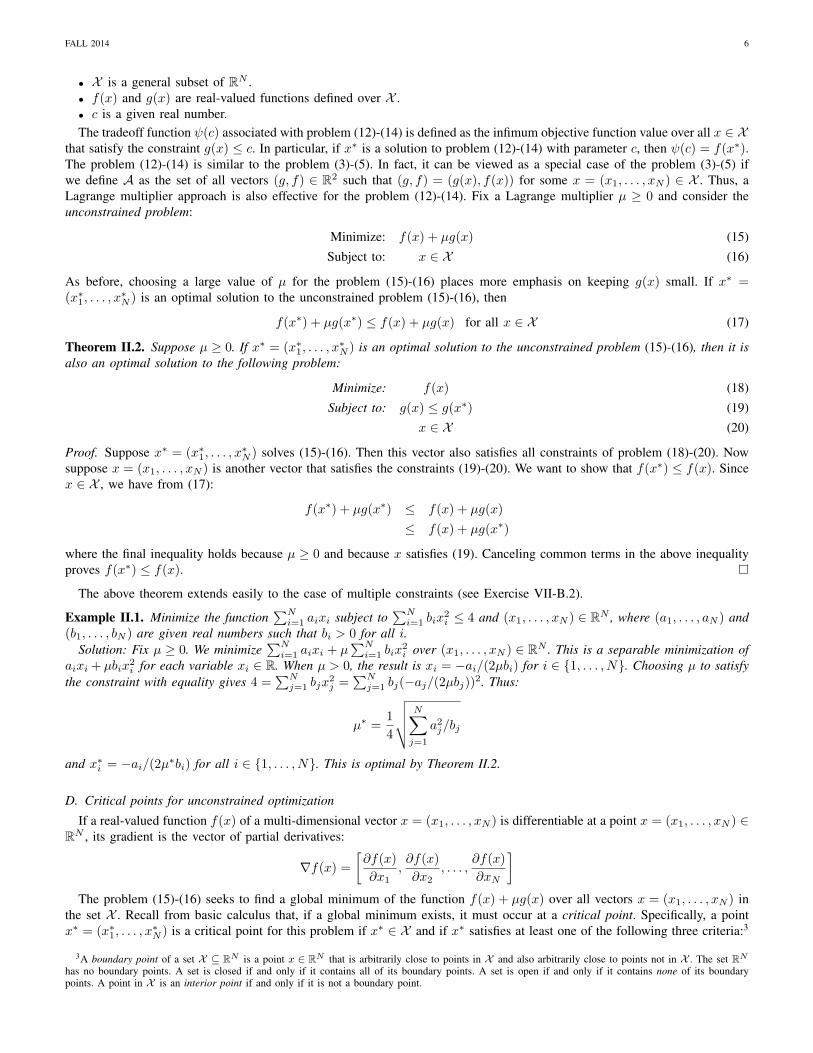
Example II.2. Define X as the set of real numbers in the interval [0, 1]. Define f(x) = x2 and g(x) = −x. Given µ ≥ 0, wewant to minimize f(x) + µg(x) over x ∈ [0, 1]. Find the critical points. Then find the optimal x∗.

Solution: The boundary points of [0, 1] are x = 0 and x = 1. The function f(x) + µg(x) is differentiable for all x. Thestationary equation is f ′(x) +µg′(x) = 2x−µ = 0. This produces a critical point x = µ/2. However, this point is only validif 0 ≤ µ ≤ 2 (since if µ > 2 then x = µ/2 > 1, which is out of the desired interval [0, 1]).

Thus, for µ ∈ [0, 2] we test the critical points x ∈ 0, 1, µ/2:

x x2 − µx for µ ∈ [0, 2]

0 01 1− µµ/2 −µ

2

4

It can be shown that −µ2/4 ≤ 1− µ for all µ ∈ R. Thus, x∗ = µ/2 whenever µ ∈ [0, 2]. If µ > 2 then the critical pointsoccur at x = 0 and x = 1 (with x2 − µx values of 0 and 1 − µ, respectively). Since 1 − µ < 0 whenever µ > 2, it followsthat x∗ = 1 whenever µ > 2. In summary:

x∗ =

µ/2 if µ ∈ [0, 2]1 if µ > 2

(21)

A simpler method that can be shown to work when minimizing a convex function h(x) over an interval x ∈ [a, b], in the casewhen h(x) is defined and differentiable over all x ∈ R and has a point z ∈ R such that h′(z) = 0, is to project z onto theinterval [a, b]:

x∗ = [z]baM=

b if z > bz if z ∈ [a, b]a if z < a

Indeed, the solution to minimizing x2 − µx over x ∈ [0, 1] is x∗ = [µ/2]10, which is the same as (21).

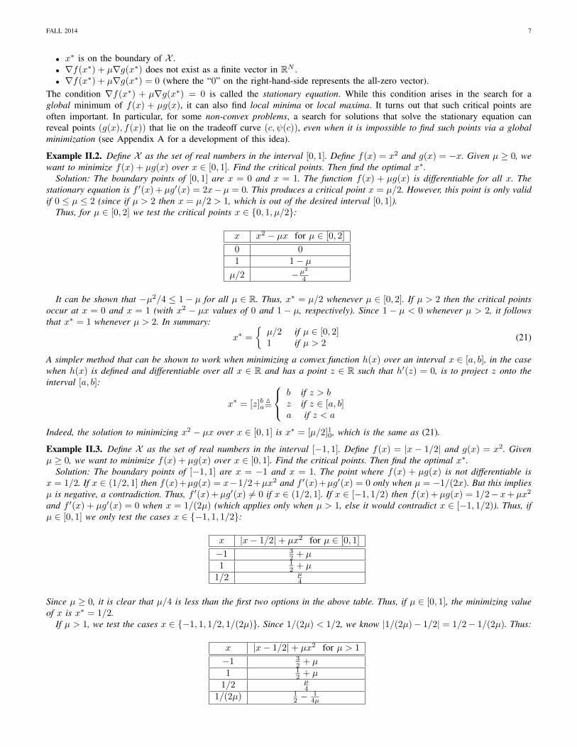
Example II.3. Define X as the set of real numbers in the interval [−1, 1]. Define f(x) = |x − 1/2| and g(x) = x2. Givenµ ≥ 0, we want to minimize f(x) + µg(x) over x ∈ [0, 1]. Find the critical points. Then find the optimal x∗.

Solution: The boundary points of [−1, 1] are x = −1 and x = 1. The point where f(x) + µg(x) is not differentiable isx = 1/2. If x ∈ (1/2, 1] then f(x)+µg(x) = x−1/2+µx2 and f ′(x)+µg′(x) = 0 only when µ = −1/(2x). But this impliesµ is negative, a contradiction. Thus, f ′(x) +µg′(x) 6= 0 if x ∈ (1/2, 1]. If x ∈ [−1, 1/2) then f(x) +µg(x) = 1/2− x+µx2

and f ′(x) + µg′(x) = 0 when x = 1/(2µ) (which applies only when µ > 1, else it would contradict x ∈ [−1, 1/2)). Thus, ifµ ∈ [0, 1] we only test the cases x ∈ −1, 1, 1/2:

x |x− 1/2|+ µx2 for µ ∈ [0, 1]

−1 32 + µ

1 12 + µ

1/2 µ4

Since µ ≥ 0, it is clear that µ/4 is less than the first two options in the above table. Thus, if µ ∈ [0, 1], the minimizing valueof x is x∗ = 1/2.

If µ > 1, we test the cases x ∈ −1, 1, 1/2, 1/(2µ). Since 1/(2µ) < 1/2, we know |1/(2µ)− 1/2| = 1/2− 1/(2µ). Thus:

x |x− 1/2|+ µx2 for µ > 1

−1 32 + µ

1 12 + µ

1/2 µ4

1/(2µ) 12 −

14µ

FALL 2014 8

The minimum is found by comparing the last two rows. Since µ > 1, it can be shown that µ4 >

12 −

14µ . Thus:

x∗ =

1/2 if µ ∈ [0, 1]1/(2µ) if µ > 1

E. Rate allocation example

Consider three devices that send data over a common link of capacity C bits/second. Let (r1, r2, r3) be the vector of datarates selected for the three devices. Define X as the set of all non-negative rate vectors in R3:

X = (r1, r2, r3) ∈ R3|r1 ≥ 0, r2 ≥ 0, r3 ≥ 0

Consider the following weighted proportionally fair rate allocation problem:

Maximize: log(r1) + 2 log(r2) + 3 log(r3)

Subject to: r1 + r2 + r3 ≤ C(r1, r2, r3) ∈ X

The weights imply that higher indexed devices have higher priority in the rate maximization. To solve, turn this into aminimization problem as follows:

Minimize: (−1)[log(r1) + 2 log(r2) + 3 log(r3)]

Subject to: r1 + r2 + r3 ≤ C(r1, r2, r3) ∈ X

The corresponding unconstrained problem (which uses a Lagrange multiplier µ ≥ 0) is:

Minimize: −[log(r1) + 2 log(r2) + 3 log(r3)] + µ[r1 + r2 + r2]

Subject to: (r1, r2, r3) ∈ X

Since X is the set of all (r1, r2, r3) that satisfy r1 ≥ 0, r2 ≥ 0, r3 ≥ 0, the above problem is separable and can be solved byseparately minimizing over each ri:• Choose r1 ≥ 0 to minimize − log(r1) + µr1. Thus, r1 = 1/µ (assuming µ > 0).• Choose r2 ≥ 0 to minimize −2 log(r2) + µr2. Thus, r2 = 2/µ (assuming µ > 0).• Chooose r3 ≥ 0 to minimize −3 log(r3) + µr3. Thus, r3 = 3/µ (assming µ > 0).Since we have a solution parameterized by µ, we can choose µ > 0 to meet the desired constraint with equality:

C = r1 + r2 + r2 = 6/µ

Thus µ = 6/C, which is indeed non-negative. Thus, Theorem II.2 ensures that this rate allocation is optimal for the originalconstrained optimization problem:

(r∗1 , r∗2 , r∗3) = (C/6, C/3, C/2)

F. Routing example

1"

2"

3"

C"

C"

C"1"

r"

x1"x2"

x3"

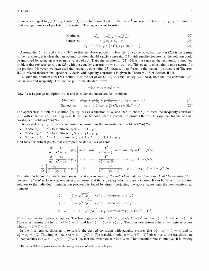
Fig. 4. A 3-queue network routing example for Subsection II-F.

Consider sending data of rate r over a choice of three parallel queues, each with a processing rate of C. The data is splitinto separate streams of rates x1, x2, x3, where data of rate xi is sent into queue i (see Fig. 4). The first two queues have noadditional traffic, while the third queue serves an additional traffic stream of rate 1. Suppose the average number of packets

FALL 2014 9

in queue i is equal to fi/(C − fi), where fi is the total arrival rate to the queue.4 We want to choose x1, x2, x3 to minimizetotal average number of packets in the system. That is, we want to solve:

Minimize: x1

C−x1+ x2

C−x2+ x3+1

C−(x3+1) (22)Subject to: r ≤ x1 + x2 + x3 (23)

x1 ∈ [0, C), x2 ∈ [0, C), x3 ∈ [0, C − 1) (24)

Assume that C > 1 and r + 1 < 3C, so that the above problem is feasible. Since the objective function (22) is increasingin the xi values, it is clear that an optimal solution should satisfy constraint (23) with equality (otherwise, the solution couldbe improved by reducing one or more values of xi). Thus, the solution to (22)-(24) is the same as the solution to a modifiedproblem that replaces constraint (23) with the equality constraint r = x1 +x2 +x3. This equality constraint is more natural forthe problem. However, we have used the inequality constraint (23) because it conforms to the inequality structure of TheoremII.2 (a related theorem that specifically deals with equality constraints is given in Theorem II.3 of Section II-H).

To solve the problem (22)-(24), define X as the set of all (x1, x2, x3) that satisfy (24). Next, note that the constraint (23)has an inverted inequality. This can be put in the standard form:

−(x1 + x2 + x3) ≤ −r

Now fix a Lagrange multiplier µ > 0 and consider the unconstrained problem:

Minimize: x1

C−x1+ x2

C−x2+ x3+1

C−(x3+1) − µ(x1 + x2 + x3) (25)

Subject to: x1 ∈ [0, C), x2 ∈ [0, C), x3 ∈ [0, C − 1) (26)

The approach is to obtain a solution (x∗1, x∗2, x∗3) as a function of µ, and then to choose µ to meet the inequality constraint

(23) with equality: x∗1 + x∗2 + x∗3 = r. If this can be done, then Theorem II.2 ensures the result is optimal for the originalconstrained problem (22)-(24).

The variables x1, x2, x3 can be optimized separately in the unconstrained problem (25)-(26):• Choose x1 ∈ [0, C) to minimize x1/(C − x1)− µx1.• Choose x2 ∈ [0, C) to minimize x2/(C − x2)− µx2.• Chosoe x3 ∈ [0, C − 1) to minimize (x3 + 1)/(C − (x3 + 1))− µx3.

First look for critical points that correspond to derivatives of zero:

d

dx

[x1

C − x1− µx1

]= 0 =⇒ C

(C − x1)2= µ =⇒ x1 = C −

√C/µ

d

dx

[x2

C − x2− µx2

]= 0 =⇒ C

(C − x2)2= µ =⇒ x2 = C −

√C/µ

d

dx

[x3 + 1

C − (x3 + 1)− µx3

]= 0 =⇒ C

(C − (x3 + 1))2= µ =⇒ x3 = C − 1−

√C/µ

The intuition behind the above solution is that the derivatives of the individual link cost functions should be equalized to acommon value of µ. However, one must also ensure that the x1, x2, x3 values are non-negative. It can be shown that the truesolution to the individual minimization problems is found by simply projecting the above values onto the non-negative realnumbers:

x∗1 =[C −

√C/µ

]+(x∗1 > 0 whenever µ > 1/C)

x∗2 =[C −

√C/µ

]+(x∗2 > 0 whenever µ > 1/C)

x∗3 =[C − 1−

√C/µ

]+(x∗3 > 0 whenever µ > C/(C − 1)2)

Thus, there are two different regimes: The first regime is when 1/C < µ ≤ C/(C − 1)2 and has x∗1 = x∗2 > 0 and x∗3 = 0.The second regime is when µ > C/(C − 1)2 and has x∗1 = x∗2 > 0, x∗3 > 0. The transition between these two regimes occurswhen µ = C/(C − 1)2.

In the first regime, choosing µ to satisfy the desired constraint with equality ensures that x∗1 + x∗2 + 0 = r, and sox∗1 = x∗2 = r/2. This implies that r/2 = C −

√C/µ. The transition point µ = C/(C − 1)2 gives rise to the transition rate

r that satisfies r/2 = C −√

(C − 1)2 = 1 (so that the transition rate is r = 2). This transition rate is intuitive: It is exactly

4This is an M/M/1 approximation for the average number of packets in each queue.

FALL 2014 10

when the derivative of the cost function of paths 1 and 2 (evaluated when x1 = x2 = 1) is equal to the derivative of the costfunction of path 3 (when x3 = 0):

d

dx1

[x1

C − x1

]x1=1

=d

dx2

[x2

C − x2

]x2=1

=d

dx3

[x3 + 1

C − (x3 + 1)

]x3=0

Thus, when 0 < r ≤ 2, the optimal solution is x∗1 = x∗2 = r/2, x∗3 = 0.On the other hand, when 2 < r < 3C − 1, the optimal solution has r = x∗1 +x∗2 +x∗3 = 2(C −

√C/µ) + (C − 1−

√C/µ).

This means that:

µ∗ = C

(3

3C − 1− r

)2

and the optimal solution is:

x∗1 = x∗2 = C −√C/µ∗ = (r + 1)/3

x∗3 = C − 1−√C/µ∗ = (r − 2)/3

This solution is intuitive because it equalizes the total input rate on each path, and hence also equalizes the individual pathderivatives:

d

dx1

[x1

C − x1

]x1=x∗

1

=d

dx2

[x2

C − x2

]x2=x∗

2

=d

dx3

[x3 + 1

C − (x3 + 1)

]x3=x∗

3

In summary, the solution to (22)-(24) is:

(x∗1, x∗2, x∗3) =

(r2 ,

r2 , 0)

if 0 < r ≤ 2(r+13 , r+1

3 , r−23)

if 2 < r < 3C − 1

G. Power allocation example

Consider a collection of N orthogonal channels. A wireless transmitter can send simultaneously over all channels usinga power vector p = (p1, . . . , pN ). For each channel i, let fi(pi) be the transmission rate over the channel. The goal is tomaximize the sum transmission rate subject to a sum power constraint of pmax (for some given value pmax > 0):

Maximize:∑Ni=1 fi(pi) (27)

Subject to:∑Ni=1 pi ≤ pmax (28)

pi ≥ 0 ∀i ∈ 1, . . . , N (29)

For this example, assume that each function fi(p) is increasing over the interval p ∈ [0, pmax]. Further assume the function isdifferentiable and has a decreasing derivative, so that if p1, p2 are in the interval [0, pmax] and if p1 < p2, then f ′(p1) > f ′(p2).Such a function fi(p) has a diminishing returns property with each incremental increase in p, and can be shown to be a strictlyconcave function (a formal definition of strictly concave is given in Section III). An example is:

fi(p) = log(1 + γip)

where γi is a positive attenuation parameter for each channel i ∈ 1, . . . , N.Converting to a minimization problem gives:

Minimize: −∑Ni=1 fi(pi) (30)

Subject to:∑Ni=1 pi ≤ pmax (31)

pi ≥ 0 ∀i ∈ 1, . . . , N (32)

The set X is considered to be the set of all (p1, . . . , pN ) that satisfy (32). The corresponding unconstrained problem, withLagrange multiplier µ ≥ 0, is:

Minimize: −∑Ni=1 fi(pi) + µ

∑Ni=1 pi

Subject to: pi ≥ 0 ∀i ∈ 1, . . . , N

This problem separates into N different minimization problems: For each i ∈ 1, . . . , N, solve the following:

Maximize: fi(pi)− µpi (33)Subject to: pi ≥ 0 (34)

where the minimization has been changed to a maximization for simplicity. Each separate problem is a simple maximizationof a function of one variable over the interval pi ∈ [0,∞). The optimal pi is either a critical point (being either the endpoint

FALL 2014 11

pi = 0 or a point with zero derivative), or is achieved at pi =∞. Because the functions fi(p) are assumed to have decreasingderivatives, it can be shown that a solution to (33)-(34) is as follows:• If f ′i(0) ≤ µ then pi = 0.• Else, if f ′i(z) = µ for some z > 0 then pi = z.• Else, if f ′i(∞) ≥ µ then pi =∞.

Assume the channels are rank ordered so that:

f ′1(0) ≥ f ′2(0) ≥ f ′3(0) ≥ · · · ≥ f ′N (0) (35)

Assume that µ is large enough so that f ′i(∞) < µ for all i, and small enough so that f ′1(0) > µ. Define K as the largestinteger such that f ′i(0) > µ for all i ∈ 1, . . . ,K. Then an optimal solution to (33)-(34) has:• f ′i(pi) = µ for i ∈ 1, . . . ,K.• pi = 0 for i ∈ K + 1, . . . , N.

The value of µ is shifted appropriately until the above solution satisfies the power constraint∑Ni=1 pi = pmax with equality.

By Theorem II.2, that value µ yields a power vector (p∗1, . . . , p∗N ) that is an optimal solution to the original constrained

optimization problem. An illustration of the solution is given in Fig. 5. The arrows in the figure show how the (p∗1, . . . , p∗N )

values move to the right as µ is pushed down.

f1’(0)'

f2’(0)'

f3’(0)'μ'

Power'p'p1' p2'

f1’(p1)'

f2’(p2)'

f3’(p3)'

Fig. 5. An illustration of the derivative requirement for optimality in the problem (27)-(29). As the value µ is pushed down, the p1 and p2 values increasealong their respective curves. Currently p3 = 0. Pushing µ below the f ′3(0) threshold activates the third curve with p3 > 0.

For a specific example, when the fi(p) = log(1 + γip) for all i, and when µ > 0, the problem (33)-(34) becomes:

Maximize: log(1 + γipi)− µpiSubject to: pi ≥ 0

The solution is:

pi =

[1

µ− 1

γi

]+(36)

where [x]+ = max[x, 0]. That is, pi > 0 if and only if 1/µ > 1/γi. In this case, the parameter 1/µ should be increased,starting from 0, until:

N∑i=1

[1

µ− 1

γi

]+= pmax (37)

When such a value µ is found, it follows from Theorem II.2 that the resulting powers pi given by (36) are optimal. The rankordering (35) implies:

γ1 ≥ γ2 ≥ · · · ≥ γN

Intuitively, this means that better channels come first in the rank ordering. For some integer K ∈ 1, . . . , N the optimalsolution has pi > 0 for i ∈ 1, . . . ,K and pi = 0 for i > K. One way to solve this is to consider all potential values of K,starting with K = N :

FALL 2014 12

• Assume K = N . Then pi > 0 for all i, and so 1/µ ≥ 1/γi for all i ∈ 1, . . . , N. The equation (37) becomes:N∑i=1

(1

µ− 1

γi

)= pmax

and so:1

µ=pmax +

∑Ni=1 1/γi

N

If this 1/µ value indeed satisfies 1/µ ≥ 1/γi for all i ∈ 1, . . . , N, we are done. Else go to the next step.• Assume K = N − 1, so that pi > 0 for i ∈ 1, . . . , N − 1 and pN = 0. Then 1/µ ≥ 1/γi for all i ∈ 1, . . . , N − 1

and 1/µ < 1/γN . The equation (37) becomes:N−1∑i=1

(1

µ− 1

γi

)= pmax

and so:1

µ=pmax +

∑N−1i=1 1/γi

N − 1

If this 1/µ value indeed satisfies 1/µ ≥ 1/γi for all i ∈ 1, . . . , N − 1, we are done. Else go to the next step.• and so on.The above procedure involves at most N steps. One can speed up the procedure by performing a bisection like search, rather

than a sequential search, which is helpful when N is large.

H. Equality constraints

Consider a problem where the inequality constraint is replaced with an equality constraint:

Minimize: f(x) (38)Subject to: g(x) = c (39)

x ∈ X (40)

where x = (x1, . . . , xN ), X ⊂ RN , and f(x) and g(x) are real-valued functions over X . The Lagrange multiplier approachconsiders the unconstrained problem defined by a parameter λ ∈ R:

Minimize: f(x) + λg(x) (41)Subject to: x ∈ X (42)

The only difference is that for equality constraints, the Lagrange multiplier λ can possibly be a negative value.

Theorem II.3. If x∗ is a solution to (41)-(42), then x∗ is also a solution to:

Minimize: f(x)

Subject to: g(x) = g(x∗)

x ∈ X

Proof. The proof is almost identical to that of Theorem II.2 and is left as an exercise (see Exercise VII-B.3).

As before, in the special case when f(x) and g(x) are differentiable over the interior of X , solutions to the stationaryequation ∇f(x) + λ∇g(x) = 0 are often useful even if they do not correspond to a global minimum of f(x) + λg(x) overx ∈ X (see Appendix A).

III. CONVEXITY

A. Convex sets

Let X be a subset of RN .

Definition III.1. A set X ⊆ RN is convex if for any two points x and y in X , the line segment between those points is alsoin X . That is, for any θ ∈ [0, 1], we have θx+ (1− θ)y ∈ X .

By convention, the empty set is considered to be convex. Likewise, a set with only one element is convex. It can be shownthat the intersection of two convex sets is still convex. Indeed, let A and B be convex sets in RN . Let x and y be two points in

FALL 2014 13

A∩B. Since both points x and y are in A, the line segment between them must also be in A (since A is convex). Similarly,the line segment must be in B. So the line segment is in A ∩ B. By the same argument, it follows that the intersection of anarbitrary (possibly uncountably infinite) number of convex sets is convex.

For a vector x = (x1, . . . , xN ) ∈ RN , define the norm ||x|| =√∑N

i=1 x2i . The set

x ∈ RN such that ||x|| = 1

is not convex because it contains the point (1, 0, 0, . . . , 0) and (−1, 0, 0, . . . , 0), but does not contain 1

2 (1, 0, 0, . . . , 0) +12 (−1, 0, 0, . . . , 0) = (0, 0, 0, . . . , 0).

Example III.1. Let a ∈ RN . Define A =x ∈ RN such that ||x− a|| ≤ 1

. The set A is convex.

Proof. Let x and y be points in A and let θ ∈ [0, 1]. We want to show that θx+ (1− θ)y ∈ A. We have:

||θx+ (1− θ)y − a|| = ||θ(x− a) + (1− θ)(y − a)||≤ ||θ(x− a)||+ ||(1− θ)(y − a)|| (43)= θ||x− a||+ (1− θ)||y − a||≤ θ + (1− θ) (44)= 1

where (43) is the triangle inequality, and (44) holds because x and y are both in A.

B. Convex sets contain their convex combinations

Let X be a subset of RN . A convex combination of points in X is a vector x of the form:

x =

k∑i=1

θixi

where k is a positive integer, x1, . . . , xk are vectors in X , and θ1, . . . , θk are non-negative numbers that sum to 1. If X isa convex set, then it contains all convex combinations of two of its points (by definition of convex). That is, if X is convexand x1, x2 are in X then (by definition of convex):

θ1x1 + θ2x2 ∈ X

whenever θ1, θ2 are non-negative and satisfy θ1 + θ2 = 1. By induction, it can be shown that if X is a convex set, then itcontains all convex combinations of its points (for any positive integer k). That is, if X is convex, if x1, . . . , xk are points inX , and if θ1, . . . , θk are non-negative numbers that sum to 1, then:

k∑i=1

θixi ∈ X (45)

The value∑ki=1 θixi can be viewed as an expectation E [X] of a random vector X that takes values in the k-element set

x1, . . . , xk with probabilities θ1, . . . , θk. Thus, if X is a convex set and X is a random vector that takes one of a finitenumber of values in X , the expression (45) means that E [X] ∈ X . This holds true more generally for random vectors X thatcan take a possibly infinite number of outcomes, where the expectation E [X] is defined either in terms of a summation overa probability mass function or an integral over a distribution function. This is formalized in the following lemma.

Lemma III.1. Let X be a random vector that takes values in a set X ⊆ RN . If X is convex and if E [X] is finite, thenE [X] ∈ X .

In the special case when the set X is closed and the expectation E [X] can be approached arbitrarily closely by a convexcombination of a finite number of points in X , then Lemma III.1 holds by (45) together with the fact that closed sets containtheir boundary points. The proof for general convex sets X is nontrivial and is omitted for brevity.5 Lemma III.1 is used toprove an inequality called Jensen’s inequality in Exercise VII-D.14.

5Lemma III.1 holds for any convex set X , regardless of whether or not it is closed and/or bounded. The proof of this fact uses the hyperplane separationtheorem for RN together with induction on the dimensionality of the problem. In particular, if E [X] is finite but is not in X , then there is a (N − 1)-dimensional hyperplane that passes through E [X] and contains X in its upper half. In particular, there is a nonzero vector γ such that γT x ≥ γTE [X] forall x ∈ X , and hence γTX ≥ γTE [X] for all realizations of the random variable X . It follows that, with probability 1, the random vector X lies on the(smaller dimensional) hyperplane for which it is known (by the induction hypothesis) that the expectation cannot leave the convex set. The assumption thatE [X] is finite is important. For example, one can define X = R (note that the set R is convex) and choose any random variable X with an infinite mean.Then X ∈ R always, but E [X] =∞ /∈ R.

FALL 2014 14

C. Convex functions

Let X ⊆ RN be a convex set. Let f : X → R be a real-valued function defined over x ∈ X .

Definition III.2. A real-valued function f(x) defined over the set X is a convex function if the set X is convex and if for allx and y in X and all θ ∈ [0, 1] we have:

f(θx+ (1− θ)y) ≤ θf(x) + (1− θ)f(y)

The function is said to be strictly convex if it is convex and if the above inequality holds with strict inequality wheneverθ ∈ (0, 1) and x 6= y.

Definition III.3. A real-valued function f(x) defined over the set X is a concave function if the set X is convex and if forall x and y in X and all θ ∈ [0, 1] we have:

f(θx+ (1− θ)y) ≥ θf(x) + (1− θ)f(y)

The function is said to be strictly concave if it is concave and if the above inequality holds with strict inequality wheneverθ ∈ (0, 1) and x 6= y.

It follows that a function f(x) defined over a convex set X is a concave function if and only if −f(x) is a convex function.Likewise, f(x) is strictly concave if and only if −f(x) is strictly convex. The set X must be convex for the definitions of aconvex function and concave function to make sense. Otherwise, the expression f(θx + (1 − θ)y) may not be defined. Thefollowing facts can be proven directly from the definition of convex:• Let c be a non-negative real number. If f(x) is a convex function, then cf(x) is also a convex function. Likewise, if g(x)

is a concave function, then cg(x) is concave.• The sum of two convex functions is convex, and the sum of two concave functions is concave.• The sum of a convex function and a strictly convex function is strictly convex.Suppose f(x) is a convex function over x ∈ R, and define f(x1, . . . , xN ) = f(x1). It can be shown that f(x1, . . . , xN ) is

a convex function over (x1, . . . , xN ) ∈ RN . However, f(x1, . . . , xN ) is not strictly convex over RN , regardless of whether ornot f(x1) is strictly convex over R (see Exercise VII-D.3). A function of the type f(x) = b + c1x1 + c2x2 + · · · + cNxN ,where b, c1, . . . , cN are given real numbers, is called an affine function. It can be shown that an affine function defined overa convex set X ⊆ RN is both a convex function and a concave function (but neither strictly convex nor strictly concave, seeExercise VII-D.4). In particular, a constant function is both convex and concave.

Lemma III.2. Suppose f1(x1), . . . , fN (xN ) are convex functions from R to R. Let x = (x1, . . . , xN ) and define f(x) =∑Ni=1 fi(xi).a) The function f(x) is convex over RN .b) The function f(x) is strictly convex if and only if all functions fi(xi) are strictly convex over R.

Proof. To prove part (a), let x = (x1, . . . , xN ) and y = (y1, . . . , yN ) be vectors in RN and let θ ∈ [0, 1]. We have:

f(θx+ (1− θ)y) =

N∑i=1

fi(θxi + (1− θ)yi)

≤N∑i=1

[θfi(xi) + (1− θ)fi(yi)]

= θf(x) + (1− θ)f(y)

where the inequality holds because each function fi(xi) is convex. This proves part (a). The proof of part (b) is an exercise(see Exercise VII-D.5).

Lemma III.3. (Convex inequality constraints) Let x = (x1, . . . , xN ) and let g1(x), . . . , gK(x) be convex functions over aconvex set X ⊆ RN . Let c1, . . . , cK be a collection of real numbers. Define A as the set of all x ∈ X that satisfy all of thefollowing constraints:

gk(x) ≤ ck for all k ∈ 1, . . . ,K

Then the set A is convex.

Proof. Exercise (see Exercise VII-D.6).

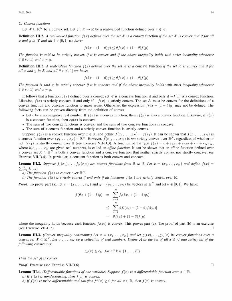
Lemma III.4. (Differentiable functions of one variable) Suppose f(x) is a differentiable function over x ∈ R.a) If f ′(x) is nondecreasing, then f(x) is convex.b) If f(x) is twice differentiable and satisfies f ′′(x) ≥ 0 for all x ∈ R, then f(x) is convex.

FALL 2014 15

c) If f(x) is twice differentiable and satisfies f ′′(x) > 0 for all x ∈ R, then f(x) is strictly convex.

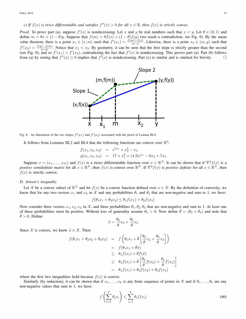
Proof. To prove part (a), suppose f ′(x) is nondecreasing. Let x and y be real numbers such that x < y. Let θ ∈ (0, 1) anddefine m = θx + (1 − θ)y. Suppose that f(m) > θf(x) + (1 − θ)f(y) (we reach a contradiction, see Fig. 6). By the meanvalue theorem, there is a point x1 ∈ (x,m) such that f ′(x1) = f(m)−f(x)

m−x . Likewise, there is a point x2 ∈ (m, y) such thatf ′(x2) = f(y)−f(m)

y−m . Notice that x1 < x2. By geometry, it can be seen that the first slope is strictly greater than the second(see Fig. 6), and so f ′(x1) > f ′(x2), contradicting the fact that f ′(x) is nondecreasing. This proves part (a). Part (b) followsfrom (a) by noting that f ′′(x) ≥ 0 implies that f ′(x) is nondecreasing. Part (c) is similar and is omitted for brevity.

x" y"m"

(y,f(y))"

(x,f(x))"

(m,f(m))"

Slope"2"

Slope"1"

x1" x2"Fig. 6. An illustration of the two slopes f ′(x1) and f ′(x2) associated with the proof of Lemma III.4.

It follows from Lemmas III.2 and III.4 that the following functions are convex over R3:

f(x1, x2, x3) = e5x1 + x22 − x3g(x1, x2, x3) = 17 + x81 + (4.2)ex1 − 6x2 + 7x3

Suppose x = (x1, . . . , xN ) and f(x) is a twice differentiable function over x ∈ RN . It can be shown that if ∇2f(x) is apositive semidefinite matrix for all x ∈ RN , then f(x) is convex over RN . If ∇2f(x) is positive definite for all x ∈ RN , thenf(x) is strictly convex.

D. Jensen’s inequalityLet X be a convex subset of RN and let f(x) be a convex function defined over x ∈ X . By the definition of convexity, we

know that for any two vectors x1 and x2 in X and any probabilities θ1 and θ2 that are non-negative and sum to 1, we have:

f(θ1x1 + θ2x2) ≤ θ1f(x1) + θ2f(x2)

Now consider three vectors x1, x2, x3 in X , and three probabilities θ1, θ2, θ3 that are non-negative and sum to 1. At least oneof these probabilities must be positive. Without loss of generality assume θ3 > 0. Now define θ = (θ2 + θ3) and note thatθ > 0. Define:

x =θ2

θx2 +

θ3

θx3

Since X is convex, we know x ∈ X . Then:

f(θ1x1 + θ2x2 + θ3x3) = f

(θ1x1 + θ

[θ2

θx2 +

θ3

θx3

])= f(θ1x1 + θx)

≤ θ1f(x1) + θf(x)

≤ θ1f(x1) + θ

[θ2

θf(x2) +

θ3

θf(x3)

]= θ1f(x1) + θ2f(x2) + θ3f(x3)

where the first two inequalities hold because f(x) is convex.Similarly (by induction), it can be shown that if x1, . . . , xk is any finite sequence of points in X and if θ1, . . . , θk are any

non-negative values that sum to 1, we have:

f

(k∑i=1

θixi

)≤

k∑i=1

θif(xi) (46)

FALL 2014 16

The above inequality is called Jensen’s inequality. A special case of Jensen’s inequality holds for time averages: Let x(t)∞t=0

be an infinite sequence of vectors in X . For slots t ∈ 1, 2, 3, . . ., define the time average:

x(t) =1

t

t−1∑τ=0

x(τ)

Then:

f(x(t)) ≤ 1

t

t−1∑τ=0

f(x(τ)) (47)

The inequality (47) is used in the development of the drift-plus-penalty algorithm for convex programs.A more general form of Jensen’s inequality is as follows: Let X be a convex set and let f(x) be a convex function over X . Let

X be a random vector that takes values in the set X and that has finite mean E [X]. Then E [X] ∈ X and f(E [X]) ≤ E [f(X)].In the special case when the random vector takes a finite number of possibilities x1, . . . , xk with probabilities θ1, . . . , θk, thenthe equation f(E [X]) ≤ E [f(X)] reduces to (46). However, the equation f(E [X]) ≤ E [f(X)] holds more generally in caseswhen X can take a countably or uncountably infinite number of values (see Exercise VII-D.14).

E. Convex hulls

Let X be a subset of RN . The convex hull of X , written Conv(X ), is the set of all convex combinations of points inX (including all points in X themselves). Thus, if x ∈ Conv(X ), then x =

∑ki=1 θixi for some positive integer k, some

non-negative values θ1, . . . , θk that sum to 1, and for some vectors x1, . . . , xk that satisfy xi ∈ X for all i ∈ 1, . . . , k.It can be shown that Conv(X ) is always a convex set.6 In general, it holds that X ⊆ Conv(X ). If the set X itself is convex,

then X = Conv(X ). If two sets X and Y satisfy X ⊆ Y , then Conv(X ) ⊆ Conv(Y). It can be shown that if X is a compactset, then Conv(X ) is also a compact set.

F. Hyperplane separation

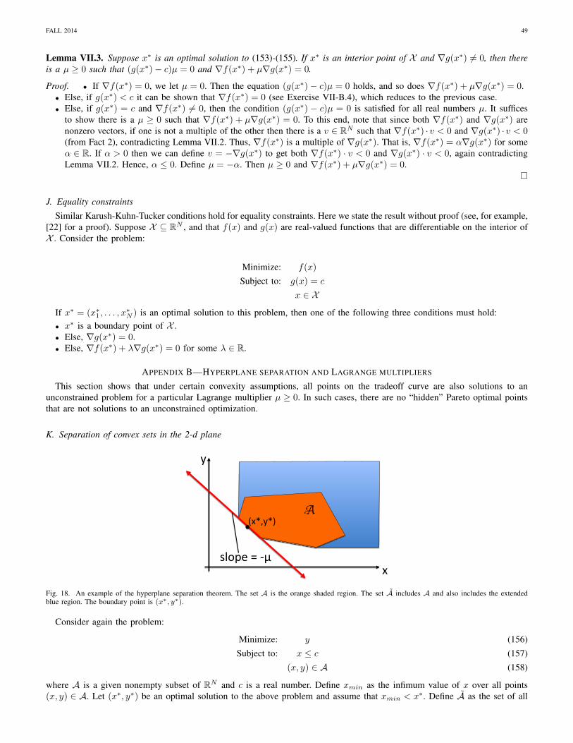
A theory of hyperplane separation for convex sets, which shows when solutions of constrained optimization problems arealso solutions of unconstrained problems with Lagrange multiplier weights, is given in Appendix B.

IV. CONVEX PROGRAMS

Let N be a positive integer. A convex program is an optimization problem that seeks to find a vector x = (x1, . . . , xN ) ∈ RNthat minimizes a convex function f(x) subject to a collection of convex constraints. Specifically, it is a problem of the form:

Minimize: f(x) (48)Subject to: gk(x) ≤ ck ∀k ∈ 1, . . . ,K (49)

x ∈ X (50)

where c1, . . . , cK are given real numbers, X is a convex subset of RN , and f(x), g1(x), . . . , gK(x) are continuous and convexfunctions from X to R. It can be shown that a convex function defined over a convex set X is continuous at every interior pointof X . Thus, the assumption that the functions f(x), g1(x), . . . , gK(x) are both convex and continuous ensures that continuityholds at all points of X , including points on the boundary.7 The convexity assumptions allow convex programs to be solvedmore easily than general constrained optimization problems. The convex program is called a linear program in the specialcase when X = RN and the functions f(x), g1(x), . . . , gK(x) are affine.

The problem is feasible if there exists an x ∈ RN that satisfies all of the constraints (49)-(50). Lemma III.3 ensures that theset of all vectors x ∈ RN that satisfy the constraints (49)-(50) is a convex set. Specifically, a constraint of the form g(x) ≤ cis called a convex constraint whenever c ∈ R and g(x) is a convex function over the set X of interest. That is because the setof all x ∈ X that satisfy this constraint forms a convex set. Since the intersection of convex sets is convex, imposing more andmore convex constraints can shrink the feasible set but maintains its convexity. It can be shown that if the problem is feasibleand if X is a compact set, then there always exists an optimal solution x∗.

Without loss of generality, one can assume all constants ck in the above convex program are zero. This is because a constraintof the form gk(x) ≤ ck is equivalent to gk(x) ≤ 0, where gk(x) is defined by gk(x) = gk(x)− ck. Note that gk(x) is convexif and only if gk(x) is convex.

6It can be shown that Conv(X ) is the “smallest” convex set that contains X , in the sense that if A is a convex set that contains X , then Conv(X ) ⊆ A.This property is sometimes used as an equivalent definition of Conv(X ). Since the intersection of an arbitrary number of convex sets is convex, the intersectionof all convex sets that contain X must be the “smallest” convex set that contains X , and so this intersection is Conv(X ).

7All convex functions f(x) defined over RN are continuous because the set RN has no boundary points. An example function f(x) defined over [0, 1]that is convex but not continuous is f(x) = 0 for x ∈ [0, 1) and f(1) = 1. Of course, the point of discontinuity occurs on the boundary of [0, 1].

FALL 2014 17

A. Equivalent forms and a network flow example

The structure (48)-(50) is the standard form for a convex program. Standard form is useful for proving results about generalconvex programs, and for developing and implementing algorithms that produce exact or approximate solutions. However,standard form is not always the most natural way of writing a convex program.

For example, consider a network that supports communication of a collection of N different traffic streams. Each trafficstream flows over its own path of links. The paths can overlap, so that some links support multiple traffic streams. Let L bethe number of links, and let Cl be the capacity of each link l ∈ 1, . . . , L. Let x = (x1, . . . , xN ) be a vector of flow rates foreach stream. Given the link capacities, the problem is to find a vector of flow rates the network can support that maximizesa concave utility function φ(x) =

∑Ni=1 log(1 + xi), which represents a measure of network fairness. This network utility

maximization problem is easily described as follows:

Maximize:∑Ni=1 log(1 + xi) (51)

Subject to:∑i∈N (l) xi ≤ Cl ∀l ∈ 1, . . . , L (52)

xi ≥ 0 ∀i ∈ 1, . . . , N (53)

where N (l) is the set of streams in the set 1, . . . , N that use link l (defined for each link l ∈ L).While the above optimization problem is not in standard form, it is correct to call it a convex optimization problem. This

is because the problem can easily be put in standard form by changing the maximization to a minimization, bringing allnon-constant terms of the inequality constraints to the left-hand-side, and/or by defining a convex set X consisting of theintersection of one or more of the constraints:

Minimize: −∑Ni=1 log(1 + xi)

Subject to:∑i∈N (l) xi ≤ Cl ∀l ∈ 1, . . . , L

x ∈ X

where X is defined as the set of all vectors x = (x1, . . . , xN ) that satisfy the constraints (53). To formally see that the aboveis now in standard form, note that X is a convex set. Further, we can define functions f(x) and gl(x) by:

f(x) = −N∑i=1

log(1 + xi)

gl(x) =∑i∈N (l)

xi ∀l ∈ 1, . . . , L

and note that these are convex and continuous functions over x ∈ X .The following structures are not in standard form, but are accepted ways of writing convex programs. That is because they

are often more natural to write than the corresponding standard form, and they can easily be put into standard form by trivialrearrangements.• Maximizing a concave function φ(x). This is equivalent to minimizing the convex function −φ(x).• Enforcing a constraint g(x) ≤ r(x) (where g(x) is convex and r(x) is concave). This is equivalent to the convex constraintg(x)− r(x) ≤ 0.

• Enforcing a constraint g(x) ≥ r(x) (where g(x) is concave and r(x) is convex). This is equivalent to the convex constraintr(x)− g(x) ≤ 0.

• Enforcing a linear equality constraint∑Ni=1 aixi = c. This is equivalent to the following two linear (and hence convex)

inequality constraints:N∑i=1

aixi − c ≤ 0

c−N∑i=1

aixi ≤ 0

• Enforcing an interval constraint xi ∈ [a, b]. This clearly imposes a convex constraint, and is equivalent to the followingtwo linear inequality constraints:

−x+ a ≤ 0

x− b ≤ 0

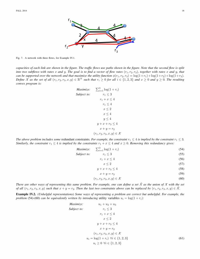
Example IV.1. Consider the network shown in Fig. 7. There are three traffic flows. Let r1, r2, r3 be the rate of each flow(in units of bits/second). Each link can support a maximum flow rate (in units of bits/second), called the link capacity. The

FALL 2014 18

4"2" 4" 4"x"y"

3" 4" 4"

r2"

r1"

r3"Fig. 7. A network with three flows, for Example IV.1.

capacities of each link are shown in the figure. The traffic flows use paths shown in the figure. Note that the second flow is splitinto two subflows with rates x and y. The goal is to find a vector of flow rates (r1, r2, r3), together with rates x and y, thatcan be supported over the network and that maximize the utility function φ(r1, r2, r3) = log(1+r1)+log(1+r2)+log(1+r3).Define X as the set of all (r1, r2, r3, x, y) ∈ RN such that ri ≥ 0 for all i ∈ 1, 2, 3 and x ≥ 0 and y ≥ 0. The resultingconvex program is:

Maximize:∑3i=1 log(1 + ri)

Subject to: r1 ≤ 3

r1 + x ≤ 4

r1 ≤ 4

x ≤ 2

x ≤ 4

y ≤ 4

y + x+ r3 ≤ 4

x+ y = r2

(r1, r2, r3, x, y) ∈ X

The above problem includes some redundant constraints. For example, the constraint r1 ≤ 4 is implied by the constraint r1 ≤ 3.Similarly, the constraint r1 ≤ 4 is implied by the constraints r1 + x ≤ 4 and x ≥ 0. Removing this redundancy gives:

Maximize:∑3i=1 log(1 + ri) (54)

Subject to: r1 ≤ 3 (55)r1 + x ≤ 4 (56)x ≤ 2 (57)

y + x+ r3 ≤ 4 (58)x+ y = r2 (59)

(r1, r2, r3, x, y) ∈ X (60)

There are other ways of representing this same problem. For example, one can define a set X as the union of X with the setof all (r1, r2, r3, x, y) such that x+ y = r2. Then the last two constraints above can be replaced by (r1, r2, r3, x, y) ∈ X .

Example IV.2. (Unhelpful representations) Some ways of representing a problem are correct but unhelpful. For example, theproblem (54)-(60) can be equivalently written by introducing utility variables ui = log(1 + ri):

Maximize: u1 + u2 + u3

Subject to: r1 ≤ 3

r1 + x ≤ 4

x ≤ 2

y + x+ r3 ≤ 4

x+ y = r2

(r1, r2, r3, x, y) ∈ Xui = log(1 + ri) ∀i ∈ 1, 2, 3 (61)

ui ≥ 0 ∀i ∈ 1, 2, 3

FALL 2014 19

However, the above representation is not a convex program because the constraints (61) are not convex (recall that equalityconstraints are convex only when both sides are affine functions of the optimization variables). One can fix the problem, whilestill keeping the ui variables, by changing the non-convex constraints (61) to the convex constraints ui ≤ log(1 + ri) forall i ∈ 1, 2, 3. This does not change the set of solutions because an optimal solution must meet the inequality constraintsui ≤ log(1 + ri) with equality. Indeed, any candidate solution that satisfies all constraints but has ui < log(1 + ri) for somei ∈ 1, 2, 3 can be strictly improved, without violating the constraints, by increasing ui to log(1 + ri).

B. Linear programs

When X = RN and the functions f(x), g1(x), . . . , gK(x) are affine, the convex program (48)-(50) has the form:

Minimize: c0 +∑Ni=1 cixi

Subject to:∑Ni=1 aikxi ≤ bk ∀k ∈ 1, . . . ,K

(x1, . . . , xN ) ∈ RN

for some given real numbers c0, c1, . . . , cN , aik for i ∈ 1, . . . , N and k ∈ 1, . . . ,K, and bk for k ∈ 1, . . . ,K. Ofcourse, c0 does nothing but shift up the value of the objective function by a constant, and so the solution to the above problemis the same as the solution to a modified problem where c0 is removed:

Minimize:∑Ni=1 cixi

Subject to:∑Ni=1 aikxi ≤ bk ∀k ∈ 1, . . . ,K

(x1, . . . , xN ) ∈ RN

It is often easier to represent the above problem in matrix form: Let c = (c1, . . . , cN ) be a column vector, let b = (b1, . . . , bK) bea column vector, and let A = (aik) be a K×N matrix. Let the variables be represented by a column vector x = (x1, . . . , xN ).The problem is then:

Minimize: cTx

Subject to: Ax ≤ bx ∈ RN

where cTx is the inner product of c and x, and the inequality Ax ≤ b is taken row-by-row.

V. THE DRIFT-PLUS-PENALTY ALGORITHM FOR CONVEX PROGRAMS

A. Convex programs over compact sets

Let x = (x1, . . . , xN ) represent a vector in RN . Consider the following convex program:

Minimize: f(x) (62)Subject to: gk(x) ≤ ck ∀k ∈ 1, . . . ,K (63)

x ∈ X (64)

where:8

• X is a convex and compact subset of RN . Recall that a subset of RN is said to be compact if it is closed and bounded.• Functions f(x), g1(x), . . . , gK(x) are continuous and convex functions over x ∈ X .• ck values are given real numbers (possibly 0).The only significant difference between the above problem and a general convex program is that the set X here is assumed

to be both convex and compact, rather than just convex. The compactness assumption ensures that an optimal solution existswhenever the problem is feasible (that is, whenever it is possible to satisfy all constraints (63)-(64)). Compactness is alsouseful because it restricts the search for an optimal solution to a bounded region of RN .

Assume the constraints are feasible. Define x∗ as an optimal solution to the above problem. Define f∗ = f(x∗) as theoptimal objective function value. A vector x ∈ X is called an ε-approximation of the solution if:

f(x) ≤ f∗ + ε

gk(x) ≤ ck + ε ∀k ∈ 1, . . . ,K

We say that x is an O(ε)-approximation if the “ε” values in the above inequalities are replaced by a constant multiple of ε.The following subsections develop an algorithm that produces an O(ε)-approximation to the convex program, for any desired

8There is no loss of generality in assuming that the ck values are all zero, since the gk(x) functions can simply be modified to gk(x) = gk(x)− ck .

FALL 2014 20

value ε > 0. The convergence time of the algorithm is O(1/ε3) in general cases, and is O(1/ε2) under the mild assumptionthat a Lagrange multiplier vector exists (see Section V-G). A modified algorithm with a delayed start mechanism has O(1/ε)convergence time under additional assumptions [6].

B. Virtual queues

The drift-plus-penalty algorithm is a method for choosing values x(t) = (x1(t), . . . , xN (t)) ∈ X over a sequence of timeslots t ∈ 0, 1, 2, . . . so that the time average x(t) = (x1(t), . . . , xN (t)) converges to a close approximation of the solutionto a particular optimization problem. The algorithm is developed in [3] for more general stochastic problems, and has closeconnections to optimization for queueing networks. These notes consider the drift-plus-penalty algorithm in the special caseof the (non-stochastic) convex program (62)-(64).

Recall that the time average x(t) is defined for all t ∈ 1, 2, 3, . . . by:

x(t) =1

t

t−1∑τ=0

x(τ)

For each constraint k ∈ 1, . . . ,K, define a virtual queue Qk(t) with update equation:

Qk(t+ 1) = max[Qk(t) + gk(x(t))− ck, 0] (65)

with initial condition Qk(0) = 0 for all k ∈ 1, . . . ,K. The value gk(x(t)) acts as a virtual arrival to the queue, and the valueck acts as a virtual service rate (per slot). In a physical queueing system the arrivals and service rate are always non-negative.However, in this virtual queue, these values gk(x(t)) and ck might be negative. If the queue Qk(t) is “stable,” so that the longterm departure rate is equal to the long term arrival rate, then the time average of the arrival process gk(x(t)) must be lessthan or equal to the service rate ck. By Jensen’s inequality, this implies that the limiting value of gk(xk(t)) is also less thanor equal to ck. Thus, stabilizing the virtual queue ensures that the desired inequality constraint is satisfied. This observation isformalized in the following lemma.

Lemma V.1. (Virtual queues) Under the queue update (65) we have for every slot t > 0 and for all k ∈ 1, . . . ,K:

gk(x(t)) ≤ ck +Qk(t)

t

Proof. Fix k ∈ 1, . . . ,K. The equation (65) for a given slot τ implies:

Qk(τ + 1) ≥ Qk(τ) + gk(x(τ))− ck

Rearranging terms gives:Qk(τ + 1)−Qk(τ) ≥ gk(x(τ))− ck

Summing the above inequality over τ ∈ 0, 1, . . . , t− 1 (for some slot t > 0) gives:

Qk(t)−Qk(0) ≥t−1∑τ=0

gk(x(τ))− ckt

Dividing by t and using the fact that Qk(0) = 0 gives:

Qk(t)

t≥ 1

t

t−1∑τ=0

gk(x(τ))− ck

Using Jensen’s inequality (47) gives:Qk(t)

t≥ gk(x(t))− ck

The value Qk(t)/t can be viewed as a bound on the constraint violation of constraint k up to slot t. The above lemmaimplies that if we control the system to ensure that limt→∞Qk(t)/t = 0 for all k ∈ 1, . . . ,K, then all desired constraintsare asymptotically satisfied:9

limt→∞

gk(x(t)) ≤ ck

A queue that satisfies Qk(t)/t→ 0 is called rate stable. Thus, the goal is to make all queues rate stable. More importantly, ifwe can control the system to maintain a finite worst-case queue size Qmax, then the constraint violations decay like Qmax/tas time progresses.

9More formally, the result is that lim supt→∞ gk(x(t)) ≤ ck .

FALL 2014 21

C. Lyapunov optimization

Define L(t) = 12

∑Kk=1Qk(t)2 as the sum of squares of all virtual queues (divided by 2 for convenience). This is called a

Lyapunov function. The value L(t) is a scalar measure of the current queue backlogs. To ensure rate stability of all queues, it isdesirable to make decisions that push L(t) down as much as possible from one slot to the next. Define ∆(t) = L(t+1)−L(t)as the Lyapunov drift, being the difference in L(t) over one slot. The drift-plus-penalty algorithm chooses x(t) ∈ X every slott to minimize a bound on the following drift-plus-penalty expression [3]:

∆(t) + V f(x(t))

where V is a non-negative parameter that affects the amount to which we consider minimization of the penalty term f(x(t)).Intuitively, we want to make ∆(t) small to ensure low queue backlogs. On the other hand, we also want to make f(x(t)) small toensure a small value of the objective function. These two goals are managed by minimizing the weighted sum ∆(t)+V f(x(t)).It will be shown that the parameter V affects a performance tradeoff between distance to the optimal objective function valueand the convergence time required to satisfy the desired constraints.

The first step is to compute a bound on ∆(t). We have for each queue k ∈ 1, . . . ,K:

Qk(t+ 1)2 = max[Qk(t) + gk(x(t))− ck, 0]2

≤ (Qk(t) + gk(x(t))− ck)2

= Qk(t)2 + (gk(x(t))− ck)2 + 2Qk(t)(gk(x(t))− ck)

Therefore:1

2[Qk(t+ 1)2 −Qk(t)2] ≤ 1

2(gk(x(t))− ck)2 +Qk(t)(gk(x(t))− ck)

Summing the above over k ∈ 1, . . . ,K gives:

∆(t) ≤ 1

2

K∑k=1

(gk(x(t))− ck)2 +

K∑k=1

Qk(t)(gk(x(t))− ck)

Define B as an upper bound on the worst-case value of 12

∑Kk=1(gk(x(t))− ck)2. This value B is finite because the set X is

assumed to be compact and the functions gk(x) are continuous. Then:

∆(t) ≤ B +

K∑k=1

Qk(t)(gk(x(t))− ck)

Adding V f(x(t)) to both sides gives the following important drift-plus-penalty inequality:

∆(t) + V f(x(t)) ≤ B + V f(x(t)) +

K∑k=1

Qk(t)[gk(x(t))− ck] (66)

The drift-plus-penalty algorithm is designed to operate as follows: Every slot t, all queues Qk(t) are observed. Then, thecontroller makes a greedy decision by selecting x(t) ∈ X to minimize the right-hand-side of (66).

Drift-plus-penalty algorithm: Every slot t ∈ 0, 1, 2, . . ., observe Q1(t), . . . , QK(t) and perform the following:• Choose x(t) ∈ X to minimize:

V f(x(t)) +∑Kk=1Qk(t)gk(x(t)) (67)

• Update the virtual queues Qk(t) via (65).It is important to emphasize that, on slot t, the values Q1(t), . . . , QK(t) are treated as known constants that act as weights in

the expression (67). Given these weights for slot t, the expression is minimized by searching over all x(t) ∈ X . The minimizerx(t) is used in the queue update equation to compute the new weights Q1(t+ 1), . . . , QK(t+ 1) for the next slot.

D. Example convex program

Consider the following example convex program, stated in terms of optimization variables x and y:

Minimize: ex + y2 (68)Subject to: x+ y ≥ 4 (69)

x+ 3y ≥ 6 (70)x ∈ [0, 5], y ∈ [0, 5] (71)

FALL 2014 22

While this problem can easily be solved by hand, it is instructive to show the steps of the drift-plus-penalty algorithm. Theproblem is equivalent to the following problem that inverts the inequality constraints (69)-(69):

Minimize: ex + y2 (72)Subject to: −x− y ≤ −4 (73)

−x− 3y ≤ −6 (74)x ∈ [0, 5], y ∈ [0, 5] (75)

Let X be the set of all (x, y) that satisfy constraints (75) (this set is a square and is indeed a convex and compact set).There are two additional constraints (73)-(74), each will receive its own virtual queue. Notice that all non-constant terms ofthe constraints (73)-(74) have been shifted to the left-hand-side, as required. The drift-plus-penalty algorithm reduces to thefollowing:

Virtual queues: Define Q1(0) = Q2(0) = 0. Variables x(t), y(t) are used in the following queue update equations every slott ∈ 0, 1, 2, . . .:

Q1(t+ 1) = max[Q1(t)− x(t)− y(t) + 4, 0] (76)Q2(t+ 1) = max[Q2(t)− x(t)− 3y(t) + 6, 0] (77)

Variable selection: Every slot t ∈ 0, 1, 2, . . ., observe Q1(t), Q2(t) and choose (x(t), y(t)) ∈ X to minimize:

V (ex(t) + y(t)2) +Q1(t)(−x(t)− y(t)) +Q2(t)(−x(t)− 3y(t))

This is a correct answer, but not complete. That is because a complete answer should exploit separable optimization in thevariable selection whenever possible. By rearranging terms, the variable selection decision corresponds to the following:

Minimize:(V ex(t) − (Q1(t) +Q2(t))x(t)

)+(V y(t)2 − (Q1(t) + 3Q2(t))y(t)

)Subject to: x(t) ∈ [0, 5], y(t) ∈ [0, 5]

It is apparent that x(t) and y(t) can be optimized separately:• x(t) selection: Choose x(t) ∈ [0, 5] to minimize V ex(t) − (Q1(t) +Q2(t))x(t). Thus:

x(t) =

[log

(Q1(t) +Q2(t)

V

)]50

(78)

where [a]50 represents a projection of the real number a onto the interval [0, 5].• y(t) selection: Choose y(t) ∈ [0, 5] to minimize V y(t)2 − (Q1(t) + 3Q2(t))y(t). Thus:

y(t) =

[Q1(t) + 3Q2(t)

2V

]50

(79)

Deterministic queue bounds: Exercise VII-F.5 shows that, in this example, there are constants β1, β2, C1, C2 such thatQ1(t) ≤ β1V +C1 and Q2(t) ≤ β2V +C2 for all t. Substituting this deterministic queue bound into Lemma V.1 implies thatfor all t ∈ 1, 2, 3, . . .:

−x(t)− y(t) ≤ −4 + (β1V + C1)/t

−x(t)− 3y(t) ≤ −6 + (β2V + C2)/t

Thus, the vector (x(t), y(t)) is very close to satisfying the desired constraints when t is large relative to V .Discussion: Choosing the set X as the square corresponding to constraints (75) was convenient as it led to a simple separable

optimization for x(t) and y(t). To produce the simplest algorithm for multi-dimensional problems, a rule of thumb is to set Xas a multi-dimensional hyper-rectangle so that each variable is restricted to a particular interval. However, this is not necessaryfor the algorithm, as shown in the next subsection.

E. Choosing a different set XConsider the same problem (72)-(75). However, now define X as the set of all (x, y) that satisfy the constraints (74)-(75).

This is the intersection of the compact square [0, 5] × [0, 5] with the convex set defined by constraint −x − 3y ≤ −6. Theresulting set is still convex and compact, but is no longer a square. The only remaining constraint in the problem is (73) (beingthe constraint −x− y ≤ −4). Thus, the drift-plus-penalty algorithm uses only one virtual queue:

Virtual queue: Define the virtual queue Q(t) with update equation:

Q(t+ 1) = max[Q(t)− x(t)− y(t) + 4, 0]

FALL 2014 23

Variable selection: Every slot t ∈ 0, 1, 2, . . ., observe Q(t) and choose (x(t), y(t)) ∈ X to minimize:

V (ex(t) + y(t)2) +Q(t)(−x(t)− y(t))

This reduces to the following problem every slot t:

Minimize:(V ex(t) −Q(t)x(t)

)+(V y(t)2 −Q(t)y(t)

)Subject to: x(t) ∈ [0, 5], y(t) ∈ [0, 5], x(t) + 3y(t) ≥ 6

While the objective function in the above minimization is still a separable sum of terms involving x(t) and y(t), the constraintx(t) + 3y(t) ≥ 6 couples the (x(t), y(t)) selection, so that these variables cannot be chosen separately. One can obtain a(non-separable) solution to the above problem by using a Lagrange multiplier on the constraint x(t) + 3y(t) ≥ 6.

The performance theorem of the next subsection ensures that time averages (x(t), y(t)) from both the algorithm in thissubsection and the algorithm in the previous subsection approach the same optimal solution to problem (68)-(71) as V →∞.

F. Performance theorem

Define Q(t) = (Q1(t), . . . , QK(t)), and define ||Q(t)|| =√∑K

i=1Qi(t)2. The following theorem is a special case of results

for more general stochastic problems in [3].

Theorem V.1. If the convex program (62)-(64) is feasible, then the drift-plus-penalty algorithm ensures:(a) f(x(t)) ≤ f∗ +B/V for all slots t ∈ 1, 2, 3, . . ..

(b) limt→∞Qk(t)t = 0 for all k ∈ 1, . . . ,K.

(c) lim supt→∞ gk(x(t)) ≤ ck for all k ∈ 1, . . . ,K.10

(d) ||Q(t)||/t ≤ O(√V/t).

Proof. (Theorem V.1 part (a)) Since the drift-plus-penalty algorithm chooses x(τ) ∈ X to minimize the right-hand-side of (66)on each slot τ , and the optimal solution x∗ is also a point in X , we have:

∆(τ) + V f(x(τ)) ≤ B + V f(x∗) +

K∑k=1

Qk(τ)(gk(x∗)− ck) (80)

≤ B + V f∗ (81)

where the final inequality holds because f(x∗) = f∗ and gk(x∗) ≤ ck for all k. Summing the above over τ ∈ 0, . . . , t− 1gives:

L(t)− L(0) + V

t−1∑τ=0

f(x(τ)) ≤ Bt+ V f∗t

Dividing by V t and using the fact that L(0) = 0 gives:

L(t)

V t+

1

t

t−1∑τ=0

f(x(τ)) ≤ B

V+ f∗ (82)

Using L(t) ≥ 0 and Jensen’s inequality (47) gives:

f(x(t)) ≤ B

V+ f∗

Proof. (Theorem V.1 parts (b)-(d)) From (82) we have for all t ∈ 1, 2, 3, . . .:L(t)

V t+ fmin ≤

B

V+ f∗

10The “lim sup” can be replaced by “lim” whenever the regular limit exists. The value lim supt→∞ h(t) exists (possibly being ∞ or −∞) for anyreal-valued function h(t), and is the largest limiting value over any subsequence of times tk that increase to infinity and for which the regular limit of h(tk)exists. For example, limt→∞ cos(t) does not exist, but lim supt→∞ cos(t) = 1. Indeed, note that no subsequence of times tk can have a limiting value ofcos(tk) that is larger than 1, but one can define the particular subsequence tk = 2πk (for positive integers k) that satisfies limk→∞ cos(tk) = 1. If h(t) isa real valued function and if c is a real number, the statement “lim supt→∞ h(t) ≤ c” is equivalent to the statement that “for all ε > 0, there is a time Tεsuch that h(t) ≤ c+ ε whenever t ≥ Tε.” It is also equivalent to the statement that “limt→∞max[h(t), c] = c.” If two functions h1(t) and h2(t) satisfyh1(t) ≤ h2(t) for all t ≥ 0, it can be shown that lim supt→∞ h1(t) ≤ lim supt→∞ h2(t).

FALL 2014 24

where fmin = infx∈X f(x). The value fmin is finite because X is compact and f(x) is continuous. Rearranging terms gives:

L(t) ≤ Bt+ (f∗ − fmin)V t

Substituting the definition L(t) = 12 ||Q(t)||2 gives;

||Q(t)||2 ≤ 2[B + (f∗ − fmin)V ]t

Thus:||Q(t)||

t≤√

2[B + (f∗ − fmin)V ]

t

This proves part (d). Part (d) immediately proves part (b). Part (b) with Lemma V.1 proves part (c).

The theorem shows that V can be chosen as large as desired to ensure f(x(t)) is arbitrarily close to the optimal value f∗,with a corresponding tradeoff in the time required for the constraints to be close to being satisfied. Choosing V = 1/ε yields anO(ε)-approximation. The time required for the constraints to be satisfied within O(ε) is the time t such that ||Q(t)||/t ≤ O(ε).From part (d) of the above theorem, this is ensured if

√V/t ≤ ε. If V = 1/ε, it follows that we need time t ≥ 1/ε3. However,

the bound in part (d) is overly conservative. An improved convergence time bound of O(1/ε2) is given in the next subsectionunder an assumption that a Lagrange multiplier vector exists. Recent work in [6] shows that convergence time can be furtherpushed to O(1/ε) under additional assumptions and by starting the time average after some later time T > 0.

The above drift-plus-penalty theorem is developed in a more general stochastic context in [3]. Applications to distributedconvex programming are in [7]. In the (deterministic) convex program context, the drift-plus-penalty algorithm is similar tothe dual subgradient algorithm [1]. However, the dual subgradient algorithm does not take time averages and requires morestringent strict convexity assumptions for its mathematical analysis.

G. Improved convergence time analysis

Theorem V.1 only requires the convex program (62)-(64) to be feasible. The following theorem provides a tighter convergencetime analysis under the additional assumption that a Lagrange multiplier vector exists. Specifically, assume there exists a vectorµ = (µ1, . . . , µK) such that µk ≥ 0 for all k ∈ 1, . . . ,K, and:

f(x) +

K∑k=1

µkgk(x) ≥ f(x∗) +

K∑k=1

µkck ∀x ∈ X (83)

This Lagrange multiplier assumption is equivalent to the existence of a non-vertical hyperplane that is tangent to a certainconvex set, as discussed in detail in Appendix B. The following theorem is from [4].

Theorem V.2. (Improved convergence time [4]) Suppose the convex program (62)-(64) is feasible and that a Lagrange multipliervector µ = (µ1, . . . , µk) exists (so that (83) holds). Then the drift-plus-penalty algorithm with V ≥ 0 and initial conditionsQk(0) = 0 for all k ∈ 1, . . . ,K ensures:

(a) f(x(t)) ≤ f∗ + BV for all slots t ∈ 1, 2, 3, . . ., where B is the constant used in (66).

(b) ||Q(t)||t ≤ V ||µ||+

√V 2||µ||2+2Bt

t for all t ∈ 1, 2, 3, . . ..(c) Define V = 1/ε. Then for any integer t ≥ 1/ε2 we have:

f(x(t)) ≤ f∗ +O(ε)

gk(x(t)) ≤ ck +O(ε) ∀k ∈ 1, . . . ,Kx(t) ∈ X

Hence, the drift-plus-penalty algorithm produces an O(ε) approximation to the solution with a convergence time of O(1/ε2).

Proof. Part (a) is already known from Theorem V.1. Part (c) follows immediately from parts (a) and (b) together with LemmaV.1. Part (b) is proven in Appendix C.

H. Choosing the set X for general problems

Consider the convex program (62)-(64), which seeks to minimize f(x) subject to gk(x) ≤ ck for all k ∈ 1, . . . ,K andx ∈ X (where X is a convex set and f(x), gk(x) are convex functions). Now define X as the intersection of X and the setof all x ∈ RN that satisfy gK(x) ≤ cK . Since the intersection of convex sets is convex, the set X is convex. The originalproblem (62)-(64) is equivalent to the following:

Minimize: f(x)

Subject to: gk(x) ≤ ck ∀k ∈ 1, . . . ,K − 1x ∈ X

FALL 2014 25

The only difference is that the above convex program is written by shifting the last constraint gK(x) ≤ cK into the set constraintx ∈ X . While this does not change the underlying problem, it gives rise to a different implementation of the drift-plus-penaltyalgorithm that uses one fewer virtual queue and that seeks to find x(t) ∈ X to minimize:

V f(x(t)) +

K−1∑k=1

Qk(t)gk(x(t))

The advantage of using one less virtual queue is that the constant B in Theorem V.1 is now smaller. Intuitively, the algorithmprovides tighter performance at the cost of doing a search for x(t) over the more complex set X , rather than the larger (buttypically simpler) set X . Indeed, in the extreme case, one can place all constraints gk(x) ≤ ck into an abstract set X ′. Thatis, we can define X ′ as the intersection:

X ′ = X ∩∩Kk=1x ∈ RN |gk(x) ≤ ck

The resulting drift-plus-penalty algorithm then uses no virtual queues, and converges to the correct answer immediately onslot 0. Of course, this is because it is forced to choose x(0) ∈ X ′ as the minimizer of f(x), which is identical to choosingx(0) as the optimal solution to the original convex program!

One can write a single convex program in multiple ways. In practice, one should choose the abstract set X , and thecorresponding constraints gk(x) ≤ ck that are not incorporated into X , in such a way that searching over x ∈ X to minimizeV f(x) +

∑Kk=1Qk(t)gk(x) is easy. A rule of thumb is to choose X as a hyper-rectangle whenever possible, so that it has the

form:X = x ∈ RN |xi,min ≤ xi ≤ xi,max ∀i ∈ 1, . . . , N

for some real numbers xi,min and xi,max. This is especially useful when the functions f(x) and gk(x) are separable sums ofthe individual xi variables. For example, suppose that:

f(x) =

N∑i=1

fi(xi)

gk(x) =

N∑i=1

gki(xi) ∀k ∈ 1, . . . ,K

for some convex functions fi(xi) and gki(xi). In this case, the drift-plus-penalty algorithm of choosing x(t) ∈ X to minimizeV f(x(t)) +

∑Kk=1Qk(t)gk(x(t)) is reduced to separately choosing each variable xi(t), for each i ∈ 1, . . . , N, to solve:

Minimize: V fi(xi(t)) +∑Kk=1Qk(t)gki(xi(t))

Subject to: xi(t) ∈ [xi,min, xi,max]

This is a minimization of a convex function of one variable over an interval. The minimum occurs at a critical point: either aboundary point xi,min or xi,max, a point where the derivative does not exist, or a point of zero derivative. Often, the optimalchoice of xi(t) can be solved in closed form. This is the case for linear programs, where the functions f(x) and gk(x) areaffine (see Exercise VII-F.1). This separable property is particularly useful for distributed implementation in systems wheredifferent devices choose different xi(t) values. Separability can often be designed by creating local estimation variables tofacilitate distributed implementation (see [7] and Exercises VII-F.15-VII-F.17).

I. A small network example

dest%x1%

a%

b%

c%

x2%Fig. 8. A small network example for Subsection V-I.

Consider the following example exercise: A network with two flows must be optimized for maximum utility subject topower constraints (see Fig. 8). The flow rates are x1, x2 and are chosen over intervals x1 ∈ [0, xmax] and x2 ∈ [0, xmax],

FALL 2014 26

where xmax is some given positive number that bounds the maximum flow rate. The total power (summed over all links) isef1 +ef2 +ef3 +ef4 +ef5−5, where fl is the total flow rate over link l, defined for each l ∈ 1, . . . , 5. We want to maximizethe utility function log(1+x1)+log(1+x2) subject to a total power constraint of ptot (where ptot is a given positive constant):

ef1 + ef2 + ef3 + ef4 + ef5 − 5 ≤ ptotThe convex optimization problem is to choose input rates x1, x2 and flow rates a, b, c to solve:

Maximize: log(1 + x1) + log(1 + x2) (84)Subject to: a+ b+ c ≥ x1 (85)

h(x1, x2, a, b, c) ≤ ptot (86)a, b, c, x1, x2 ∈ [0, xmax] (87)

a) Define the convex function h(x1, x2, a, b, c) that defines total power used in the network.b) Let X be the set described by constraint (87). State all virtual queues for this problem.c) Using answers from parts (a)-(b), state the drift-plus-penalty algorithm for this problem. Make sure to exactly specify all

choices of the decision variables, and to exploit separable structure whenever possible. Explicitly solve in closed form for anyvariables that are completely separable.

Solution:a) We have h(x1, x2, a, b, c) = 2ea + eb + ec + ec+x2 − 5. This is indeed a convex function of (x1, x2, a, b, c).b) Since X is the set of all (x1, x2, a, b, c) that satisfy (87), there are only two remaining constraints, namely, constraints

(85)-(86). We could label their virtual queues as Q1(t) and Q2(t). Alternatively, we could simply label the virtual queues asQ(t) and Z(t). Using the latter notation gives:

Q(t+ 1) = max[Q(t) + x1(t)− a(t)− b(t)− c(t), 0]

Z(t+ 1) = max[Z(t) + 2ea(t) + eb(t) + ec(t) + ec(t)+x2(t) − 5− ptot, 0]

Notice that for virtual queue Q(t), we remembered to modify the constraint (85) to a less-than-or-equal-to constraint, and toshift all non-constant terms to the left-hand-side (so the constraint is equivalent to x1 − (a+ b+ c) ≤ 0).

c) Every slot t, observe the virtual queues and choose (x1(t), x2(t), a(t), b(t), c(t)) ∈ X to minimize:

−V log(1 + x1(t))− V log(1 + x2(t)) +Q(t)(x1(t)− a(t)− b(t)− c(t))+Z(t)(2ea(t) + eb(t) + ec(t) + ec(t)+x2(t) − 5− ptot)

This reduces to choosing:• x1(t) ∈ [0, xmax] to maximize V log(1 + x1(t))−Q(t)x1(t). Thus, x1(t) = [V/Q(t)− 1]xmax

0 .• (x2(t), c(t)) ∈ [0, xmax]× [0, xmax] to minimize −V log(1 + x2(t)) + Z(t)ec(t)+x2(t) + Z(t)ec(t). Thus, x2(t) and c(t)

must be chosen together.• Choose a(t) ∈ [0, xmax] to minimize −a(t)Q(t) + 2Z(t)ea(t). Thus, choose a(t) =

[log(Q(t)2Z(t)

)]xmax

0.

• Choose b(t) ∈ [0, xmax] to minimize −b(t)Q(t) + Z(t)eb(t). Thus, b(t) =[log(Q(t)Z(t)

)]xmax

0.

J. General time averages (without convexity)

Theorem V.1 and Lemma V.1 only use convexity of f(x) and gk(x) when applying Jensen’s inequality at the every end topush a time average inside a convex function while preserving a desired inequality. No convexity assumptions are needed if onewants to optimize the time average of a function, rather than a function of a time average. Indeed, suppose Y is a closed andbounded (possibly non-convex) subset of RK+1 (possibly non-convex). Consider the following time average problem: Everytime slot t ∈ 0, 1, 2, . . ., choose a vector y(t) = (y0(t), y1(t), . . . , yK(t)) ∈ Y so that the resulting time averages solve:

Minimize: limt→∞ y0(t)

Subject to: limt→∞ yk(t) ≤ ck ∀k ∈ 1, . . . ,Kx(t) ∈ X ∀t ∈ 0, 1, 2, . . .

The general algorithm for this is as follows [3]: For each k ∈ 1, . . . ,K, define virtual queues Qk(t) by:

Qk(t+ 1) = max[Qk(t) + yk(t)− ck, 0] (88)

Every slot t, observe Q1(t), . . . , QK(t) and choose y(t) ∈ Y to minimize:

V y0(t) +

K∑k=1

Qk(t)yk(t)

Then update the queues via (88). See Exercise VII-F.12 for a simple example.

FALL 2014 27

K. Equality constraints

Again let X be a general (possibly non-convex) set and suppose x(t) ∈ X for all t ∈ 0, 1, 2, . . .. Define y0(t) = f(x(t)),yk(t) = gk(x(t)), and wm(t) = hm(x(t)) for some bounded functions f(x), gk(x), hm(x) over x ∈ X for all k ∈ 1, . . . ,Kand m ∈ 1, . . . ,M (where K and M are some non-negative integers. Consider the problem:

Minimize: limt→∞ y0(t)

Subject to: limt→∞ yk(t) ≤ 0 ∀k ∈ 1, . . . ,Klimt→∞ wm(t) = 0 ∀m ∈ 1, . . . ,M

x(t) ∈ X ∀t ∈ 0, 1, 2, . . .

The drift-plus-penalty algorithm in this context uses queues Qk(t) and Zm(t) with updates [3]:

Qk(t+ 1) = max [Qk(t) + yk(t), 0]

Zm(t+ 1) = Zm(t) + wm(t)

Every slot t ∈ 0, 1, 2, . . ., the algorithm observes Q1(t), . . . , QK(t) and Z1(t), . . . , ZM (t) and chooses x(t) ∈ X to minimize:

V y0(t) +

K∑k=1

Qk(t)yk(t) +

M∑m=1

Zm(t)wm(t)

That is, choose x(t) ∈ X to minimize the following:

V f(x(t)) +

K∑k=1

Qk(t)gk(x(t)) +

M∑m=1

Zm(t)hm(x(t))

If the f(x) and gk(x) functions are continuous and convex, the hm(x) functions are affine, and the set X is convex, thenJensen’s inequality ensures this procedure provides an O(ε)-approximation to the convex program of minimizing f(x) subjectto gk(x) ≤ 0 for all k ∈ 1, . . . ,K and hm(x) = 0 for all m ∈ 1, . . . ,M (where ε = 1/V ).

L. Stochastic problems

See [3] for a development of the drift-plus-penalty algorithm in more general scenarios, including stochastic scenarios.

VI. NETWORK OPTIMIZATION VIA DRIFT-PLUS-PENALTY

This section applies the drift-plus-penalty algorithm to general network optimization problems. Recall that the drift-plus-penalty algorithm is as follows: To solve the convex program of finding x ∈ X to minimize f(x) subject to gk(x) ≤ ck forall k ∈ 1, . . . ,K, first define virtual queues:

Qk(t+ 1) = max[Qk(t) + gk(x(t))− ck, 0] ∀k ∈ 1, . . . ,K (89)

Assume that Qk(0) = 0 for all k ∈ 1, . . . ,K. Every slot t ∈ 0, 1, 2, . . ., observe the virtual queues Qk(t) and choosex(t) ∈ X to minimize the expression:

V f(x(t)) +

K∑k=1

Qk(t)gk(x(t))

Then update the virtual queues for slot t+ 1 via (89) using the vector x(t) that was chosen on slot t.

A. Flow-based optimization

Consider a network with L links and N traffic flows. Let Cl be the capacity of link l ∈ 1, . . . , L, taking units of bits/slot(where a time slot is selected as a convenient unit of time). Assume each flow uses a pre-determined path that consists of asubset of links. Define P(i) as the subset of links used by flow i, defined for each i ∈ 1, . . . , N. Let N (l) denote the setof flows in 1, . . . , N that use link l. Let x = (x1, . . . , xN ) be the vector of flow rates, so that xi is the traffic rate of flow i(in bits/slot). We want to choose x ∈ RN to solve the following network utility maximization problem:

Maximize:∑Ni=1 φi(xi) (90)

Subject to:∑i∈N (l) xi ≤ Cl ∀l ∈ 1, . . . , L (91)

xi ∈ [0, xmax] ∀i ∈ 1, . . . , N (92)

where xmax is some maximum flow rate, and φi(x) are concave functions over x ∈ [0, xmax] for each i ∈ 1, . . . , N. Thisproblem is similar to (51)-(53) with the exception that a general concave utility function is used (not necessarily φi(x) =

FALL 2014 28

log(1 + x)) and the constraint xi ≥ 0 is changed to xi ∈ [0, xmax]. This change is important to ensure the optimizationvariables x are chosen in a compact set X . In this case, the set X is the set of all x ∈ RN that satisfy (92).

Virtual queues: For each constraint l ∈ 1, . . . , L, define a virtual queue Ql(t) with dynamics:

Ql(t+ 1) = max

Ql(t) +∑i∈N (l)

xi(t)− Cl, 0

(93)

Drift-plus-penalty algorithm: Every slot t, the network controller observes Q1(t), . . . , QL(t) and chooses x(t) ∈ X tominimize:

−VN∑i=1

φi(xi(t)) +

L∑l=1

Ql(t)

∑i∈N (l)

xi(t)

Separable implementation: The algorithm reduces to the following: Each node i ∈ 1, . . . , N chooses xi(t) ∈ [0, xmax] to

maximize:

V φi(xi(t))−

∑l∈P(i)

Ql(t)

xi(t)Define:

Wi(t) =∑l∈P(i)

Ql(t) (94)

Then xi(t) is chosen in [0, xmax] to maximize V φi(xi(t))−Wi(t)xi(t).Special case: In the special case when φi(x) = (θi/b) log(1 + bx) for all i, the decision at flow i is:

x∗i (t) =

[V θi/Wi(t)− 1

b

]xmax

0

Under this algorithm, it is not difficult to show that:

Ql(t) ≤ V θmax/b+ xmax ∀t ∈ 0, 1, 2, . . . (95)

where θmax = maxi∈1,...,N θi, provided that Ql(0) satisfies this inequality.11 Since deviation from optimal utility is likeO(1/V ), the deviation from optimality can be pushed arbitrarily small by increasing the V parameter, with a correspondingO(V ) tradeoff in queue size.

Interpretation: The virtual queueing equation (93) looks like an actual queue for link l that receives arrivals∑i∈N (l) xi(t)

on slot t, and that has a service rate Cl. This is an approximation to the actual network queueing dynamics because it assumesall new arrivals are placed immediately and simultaneously on all links of the path. Of course, the actual arrivals wouldtraverse the path one link at a time. Nevertheless, the approximation is useful and is typically a good approximation of networkperformance.

The weight Wi(t) is the sum of the current queue values along the path P(i). It is difficult to obtain the exact value ofWi(t). The value Wi(t) can be approximated by having each packet observe the queue contents in each queue of its path, andstore the accumulating sum in a header field. The resulting sum is passed as a delayed feedback message to the source of eachflow i. This provides an approximation of Wi(t) that is typically within an additive constant C from the true value, called aC-additive approximation. It can be shown that the drift-plus-penalty algorithm still works optimally with such approximations(see Exercise VII-F.11). However, the queue bounds increase with C, and the resulting value of V typically needs to increaseto achieve the same performance as the case C = 0.

The above algorithm is similar to the algorithms of [8][9], which use an alternative dual subgradient method for its derivation,and to the “Fast-TCP” implementation in [10] that bases decisions on a path price. The dual subgradient algorithm in thatcontext uses a “step size” parameter δ, and requires updates to be performed every δ units of time (optimality is approachedonly when δ → 0). In contrast, the drift-plus-penalty algorithm is implemented over fixed size slots that do not need to shrinkdown to zero. This allows a fixed amount of time for network decisions to be made and implemented, which is important inpractical situations when decisions cannot be made arbitrarily rapidly. However, the resulting decisions are identical to thoseof the dual subgradient algorithm under the change of variables V = 1/δ (so V can be viewed abstractly as an inverse stepsize parameter). There is another advantage of using a small slot size, even with the drift-plus-penalty algorithm. Indeed, ifone assumes that the maximum per-slot arrivals and service are proportional to the slot size, it is not difficult to show thatshrinking the slot size can maintain the same network utility with proportionally smaller queue sizes (see Exercise VII-F.14).In practice, one should use a slot size that is as small as possible, but no smaller than that which is physically practical.

11More generally, it can be shown that Ql(t) ≤ O(V ) for all t whenever the utility functions have a bounded maximum right-derivative [3]. Definingε = 1/V and noting that Ql(t)/t is a bound on the constraint l violation implies that Ql(t)/t ≤ O(ε) for all t ≥ Ω(1/ε2).

FALL 2014 29

The traditional dual subgradient algorithm analysis does not involve a time average, and hence requires more stringent strictconvexity assumptions on the objective function. In particular, it does not support additional routing variables for extendedproblems of multi-path routing, since those variables appear in the constraints but not in the objective function. The timeaveraging analysis in the drift-plus-penalty algorithm does not require strict convexity, and hence it can handle any convexprograms, including those with multi-path routing (see Exercise VII-F.6). Further, the time averages often have a direct physicalmeaning, such as average throughput or power.

It can be shown that using link weights that are a constant multiple of Ql(t) will still give a correct operation. That is,instead of using Wi(t), one can use Wi(t) =

∑l∈P(i) γlQl(t) for some arbitrary (but fixed) values γl > 0. This is because each

constraint l in (91) is equivalent to the corresponding constraint when both sides are multiplied by γl (see Exercise VII-F.10).This observation is of practical importance because it implies that any weight that is proportional to Ql(t) (such as the observedaverage delay on link l) will work as a useful proxy for Ql(t). Implementations such as TCP-Vegas and TCP-Reno can useweights of this form [9][10]. Indeed, packets can be marked in proportion to the queue size and/or delay experienced overeach link, or a “round trip time” can be used to estimate the sum of delays. Such values can be used as proxies for Wi(t).A more accurate proxy is the sum weight over a “half-trip-time” (using only links from source to destination) rather than around trip time. Nevertheless, variations of TCP that control flow rates as a function of such weights can often be understoodas approximate implementations of the (optimal) drift-plus-penalty algorithm (and hence, also the optimal dual subgradientalgorithm in the special case when strict convexity holds). Another practical consideration is that transport layers often use awindow-based admission structure, so that admission of a precise amount of data xi(t) can only be approximated.12

B. Power constraints

Consider the same network scenario as the previous section. Thus, there are N traffic flows, each using a fixed path throughthe network. However, for each l ∈ 1, . . . , L, assume the link transmission rate is a function of a power allocation variable:Cl = µl(pl), where µl is a concave increasing function over pl ≥ 0. Suppose the network has K nodes, and let Out(k) bethe set of links that transmit out of node k. The goal is to maximize utility subject to the additional constraints that each nodek ∈ 1, . . . ,K must maintain an average power constraint. That is, we choose flow rates x1, . . . , xN and powers p1, . . . , pLto solve:

Maximize:∑Ni=1 φi(xi) (96)

Subject to:∑i∈N (l) xi ≤ µl(pl) ∀l ∈ 1, . . . , L (97)∑l∈Out(k) pl ≤ pavk ∀k ∈ 1, . . . ,K (98)

xi ∈ [0, xmax] ∀i ∈ 1, . . . , N (99)pl ∈ [0, pmax] ∀l ∈ 1, . . . , L (100)

for some given values xmax, pmax, and some desired average power constraints pavk .Solution: To solve this, define X as the set of all (x1, . . . , xN , p1, . . . , pL) vectors that satisfy (99)-(100).Virtual queues: For each constraint l ∈ 1, . . . , L in (97), define a virtual queue Ql(t) with update:

Ql(t+ 1) = max

Ql(t) +∑i∈N (l)

xi(t)− µl(pl(t)), 0

(101)

For each constraint k ∈ 1, . . . ,K in (98), define a virtual queue Zk(t) with update:

Zk(t+ 1) = max

Zk(t) +∑

l∈Out(k)

pl(t)− pavk , 0

(102)

Drift-plus-penalty algorithm: Every slot t, observe the queues Q1(t), . . . , QL(t) and Z1(t), . . . , ZK(t) and choose xi(t) andpl(t) variables to minimize:

−VN∑i=1

φi(xi(t)) +

L∑l=1

Ql(t)

∑i∈N (l)

xi(t)− µl(pl(t))

+

K∑k=1

Zk(t)

∑l∈Out(k)

pl(t)

This reduces to the following separable algorithm:

12For example, the drift-plus-penalty analysis assumes arrivals xi(t) are chosen as any real number in the interval [0, xmax], whereas a practical systemoften must admit data in packetized units. One way to address this is to use auxiliary variables [3], which maintain packetized admissions without loss ofoptimality. Another way is to maintain virtual queues with virtual admissions equal to the real numbers xi(t), but admit actual data as packets xi(t) so that∑tτ=0 xi(t) ≤

∑tτ=0 xi(t) ≤

∑tτ=0 xi(t) + xmax for all t, where xmax is the bit size of the largest packet. This idea can also be useful for matching

idealized admission rates to actual transport layer admissions in a system that uses a window-based packet admission structure.

FALL 2014 30

• (Flow control) Each flow i chooses xi(t) ∈ [0, xmax] to maximize:

V φi(xi(t))−Wi(t)xi(t)

where Wi(t) is defined in (94).• (Power allocation) Each node k chooses powers pl(t) ∈ [0, pmax] for all l ∈ Out(k) to minimize:

−Ql(t)µl(pl(t)) + Zk(t)pl(t)

• (Queue updates) Each link l updates Ql(t) via (101). Each node k updates Zk(t) via (102).

C. Backpressure routing

The previous examples of flow allocation assume flows take fixed paths. The resulting convex programs were written tooptimize flow rates subject to link capacity constraints. This does not include an optimization over all possible network routes.In general, a network might send data from the same traffic session over multiple paths. Since the number of paths between twonodes in a network is typically exponential in the size of the network, it is not obvious how to optimize over all possibilities.Nevertheless, this can be done according to a simple convex program that involves a number of variables and constraints that ispolynomial in the network size. The key is to write flow conservation equations at each node. This is a node based approach,rather than a link based approach.

Consider a network with N nodes. The nodes are connected by directional links with capacities Cab, where (a, b) denotesa link from node a to node b. Define Cab = 0 if there is no link. Let L be the set of all links (a, b). Suppose there are Mdifferent traffic flows, with flow rates x1, . . . , xM . For each m ∈ 1, . . . ,M, define source(m) and dest(m) as the source anddestination of flow m. Different flows are said to have the same commodity if they have the same destination. That is, for eachnode c ∈ 1, . . . , N, we say that commodity c data is data that is destined for node c. Let f (c)ij be a variable that representsthe amount of commodity c data that is sent over link (i, j). The goal is to choose routing variables f (c)ij that represent afeasible way of delivering commodity c data. This holds when the f (c)ij variables satisfy the following flow conservation, linkcapacity, nonnegativity, and flow efficiency constraints:∑

m∈A(n,c)

xm +

N∑a=1

f (c)an =

N∑b=1

f(c)nb ∀n ∈ 1, . . . , N,∀c 6= n (103)

N∑c=1

f(c)ab ≤ Cab ∀(a, b) ∈ L (104)

f (c)aa = 0, f (c)ca = 0 ∀a, c ∈ 1, . . . , N (105)

f(c)ab ≥ 0 ∀a, b, c ∈ 1, . . . , N (106)

where A(n, c) is defined as the set of all flows m ∈ 1, . . . ,M such that source(m) = n and dest(m) = c. Constraints(103) are the flow conservation constraints and ensure that the total commodity c flow into a node that is not the destinationis equal to the total commodity c flow out. Constraints (104) are the link capacity constraints and ensure that the sum flowrate over a given link (a, b) does not exceed the link capacity Cab. Constraints (105) are the flow efficiency constraints andensure that the network does not use a link (a, a), and does not reinject data that has already arrived to its destination backinto the network.

For each flow m ∈ 1, . . . ,M define xmaxm as a positive value that bounds the maximum flow rate, so that xm ∈ [0, xmaxm ].Let φm(x) be a concave and increasing function over x ∈ [0, xmaxm ]. The resulting convex program is:

Maximize:∑Mm=1 φm(xm) (107)

Subject to:∑m∈A(n,c) xm +

∑Na=1 f

(c)an =

∑Nb=1 f

(c)nb ∀n ∈ 1, . . . , N,∀c 6= n (108)

xm ∈ [0, xmaxm ] ∀m ∈ 1, . . . ,M (109)Constraints (104)-(106) (110)

It can be shown that the above convex program is unchanged if the equality constraint (108) is replaced by an inequality≤, meaning that the flow rate in is less than or equal to the flow rate out. This is because node n can generate fake bits thattransmit out more than what comes in.

Queues: Define X as the set of all (xm) and (f(c)ab ) variables that satisfy (108)-(110). To treat the constraints (108), for each

pair (n, c) such that n 6= c define virtual queue Q(c)n (t) with update equation:

Q(c)n (t+ 1) = max

Q(c)n (t) +

∑m∈A(n,c)

xm(t) +

N∑a=1

f (c)an (t)−N∑b=1

f(c)nb , 0

FALL 2014 31

It can be shown that the algorithm works just as well with the following modified queueing equation, which is more physicallypractical for multihop networks:13

Q(c)n (t+ 1) = max

[Q(c)n (t)−

N∑b=1

f(c)nb , 0

]+

∑m∈A(n,c)

xm(t) +

N∑a=1

f (c)an (t) (111)

This equation ensures that the exogenous arrivals on slot t, and the endogenous arrivals from other nodes, cannot be transmittedout on the same slot in which they arrive.

Drift-plus-penalty decisions: Every slot t, the network controller observes the queues and chooses variables xm(t) andf(c)ab (t) in the set X to minimize:

−VM∑m=1

φm(xm) +∑(n,c)

Q(c)n (t)

∑m∈A(n,c)

xm(t) +

N∑a=1

f (c)an (t)−N∑b=1

f(c)nb (t)

By simple rearrangements and switching the sums, the above expression becomes:

M∑m=1

[−V φm(xm) + xm(t)Q

(dest(m))source(m)(t)

]+

∑(a,b)∈L

N∑c=1

f(c)ab (t)

[Q(c)a (t)−Q(c)

b (t)]

The value Q(c)a (t) − Q(c)

b (t) is called the differential backlog of commodity c between nodes a and b. If this value is large,there is a pressure gradient associated with commodity c data on the (a, b) link. Define:

W(c)ab (t) = Q(c)

a (t)−Q(c)b (t)

The above expression is minimized by the following separable decisions:• (Flow control) Each flow m ∈ 1, . . . ,M chooses xm(t) ∈ [0, xmaxm ] to maximize:

V φm(xm)− xm(t)Q(dest(m))source(m)(t)

This is a simple decision about flow allocation at the source that only requires knowledge of the queue backlog in thesource queue. Unlike the link-based algorithm, summing weights along a path is not required.

• (Commodity selection) Each link (a, b) observes the differential backlog W (c)ab (t) for all of its commodities c ∈ 1, . . . , N.

It then chooses the single commodity c∗ab(t) that maximizes W (c)ab (t) (breaking ties arbitrarily). This is a simple decision

that is made in a distributed way at each node.• (Transmission) Each link (a, b) does the following: If maxc∈1,...,NW

(c)ab (t) > 0, then choose f (c

∗ab(t))

ab (t) = Cab andf(c)ab (t) = 0 for all c 6= c∗ab(t). That is, the link sends the single commodity c∗ab(t) with the largest differential backlog

over the link, using the full link capacity Cab. If there is not enough data of commodity c∗ab(t) to fill up the link capacity,then fake bits are transmitted.14

The first backpressure algorithm was developed in [12] in the special case V = 0, so there was no utility optimization, noflow control, and the flow rates xm were given constants that were assumed to be supportable over the network. This wasdone using a “pure drift” approach of minimizing the Lyapunov drift ∆(t). Treatment of joint flow control and backpressurewas done in [11] [13] using a V parameter to minimize the drift-plus-penalty expression ∆(t)− V

∑Mm=1 φm(xm(t)).

A simple single-commodity backpressure example is given in Exercise VII-F.13.Experimental improvements: Note that the above algorithm achieves optimal network utility (over all possible routing

algorithms) in a distributed way and without knowing a routing table. The reason is that the backlog gradients build up,much like pressure gradients when water flows through a system of pipes, and these gradients eventually push the data inoptimal directions. However, this basic algorithm can introduce large network delay, particularly when data wanders aroundcircuitous paths before gradients build up. Two standard improvements have been observed to experimentally reduce delaydramatically:• Using augmented weights W (c)

ab (t) = Q(c)a (t)−Q(c)

b (t)+θ(G(c)a −G(c)

b ), where G(c)a is an estimate of the distance between

nodes a and c, and θ is some non-negative constant. It can be shown mathematically that any non-negative values θ andG

(c)a can be used without affecting throughput utility of the algorithm (provided that V is sufficiently large). However,

it is observed experimentally that choosing G(c)a according to distance estimates provides a significant delay reduction

[3][14][15][16].• Using Last-in-First-Out (LIFO) implementation instead of First-in-First-Out (FIFO) implementation [17][18]. This can

dramatically reduce delay of 98% of the data, at the cost of incurring a large (possibly infinite) delay of the remaining 2%

13The work in [11] starts with (111), defines a Lyapunov function, and shows that the resulting drift-plus-penalty expression still satisfies an inequality ofthe form (66).

14Intuitively, this does not limit optimality because such a situation occurs only when a queue is not in danger of instability.

FALL 2014 32

of the data.15 Intuitively, the reason is that the network has a transient phase where backpressure gradients are built outof data itself. Under LIFO, the early data that create these gradients tend to stay in the same nodes for a long (possiblyinfinite) time, while the majority of the data that arrives after this transient phase speedily traverses the network using thebackpressure gradients as a form of routing table.

D. Flow-based multi-path routing

As an alternative to backpressure routing, one can use the flow-based approach of Section VI-A, without considering variablesfor all of the exponentially many paths, by taking advantage of the fact that finding a shortest path in a directed graph can bedone in polynomial time (using, for example, a Dijkstra or Bellman-Ford algorithm). This section develops such an approach.The analysis of this section uses the time-average optimization framework of Section V-J, and was originally developed in amore general stochastic context in Chapter 4.1 of [3].

As in Section VI-A, consider a network with L links (with link capacities C1, . . . , CL) and N traffic flows. Every slott ∈ 0, 1, 2, . . ., each traffic flow i ∈ 1, . . . , N chooses an amount of data xi(t) ∈ [0, xmax] and a route matrix (1il(t)).The value xi(t) represents the amount of data (in units such as bits or packets) injected into the network layer from flow i onslot t. The route matrix (1il(t)) is a matrix that specifies the particular path used for this newly injected data, so that 1il(t) isan indicator function that is 1 if the path uses link l, and is 0 else. Thus, every slot, each session can choose a new path for itsdata. Let Pi be the set of valid paths through the network from the source of flow i to its destination. The set Pi might containonly one or two path options, or might contain all possible paths from source to destination. For each link l ∈ 1, . . . , L,define yl(t) as the amount of data injected into the network layer on slot t that will eventually use link l:

yl(t) =

N∑i=1

1il(t)xi(t)

Define time averages for all slots t > 0:

xi(t) =1

t

t−1∑τ=0

xi(τ) ∀i ∈ 1, . . . , N

yl(t) =1

t

t−1∑τ=0

yl(τ) ∀l ∈ 1, . . . , L

Each link capacity constraint can be specified in a time average sense:

limt→∞

yl(t) ≤ Cl ∀l ∈ 1, . . . , L

For each i ∈ 1, . . . , N, let φi(xi) be a concave and non-decreasing utility function defined over [0, xmax]. The time-averageoptimization problem is:

Maximize: limt→∞∑Ni=1 φi(xi(t)) (112)

Subject to: limt→∞ yl(t) ≤ Cl ∀l ∈ 1, . . . , L (113)xi(t) ∈ [0, xmax] ∀i ∈ 1, . . . , N (114)

(1il(t)) ∈ Pi ∀i ∈ 1, . . . N (115)

The above problem is almost in the form of the general time average optimization problem of Section V-J. However, theobjective (112) seeks to maximize a concave function of a vector of time averages (x1(t), . . . , xN (t)), rather than maximizethe time average of a function y0(t). Fortunately, a redundant constraint can be added to the problem to make it exactly fit theframework of Section V-J, without changing the underlying optimal solution. This is done using the auxiliary variable methodof [3]. For each i ∈ 1, . . . , N, let γi(t) be an auxiliary variable chosen in the set [0, xmax] for each slot t. Define:

y0(t) =

N∑i=1

φi(γi(t)) (116)

15There is nothing fundamental about the number 0.98 in this context. For any δ > 0, the V parameter can be chosen sufficiently large to ensure the rateof packets with large delay is at most δ.

FALL 2014 33

Consider the modified problem:

Maximize: limt→∞ y0(t) (117)Subject to: limt→∞ yl(t) ≤ Cl ∀l ∈ 1, . . . , L (118)

γi(t) ≤ xi(t) ∀i ∈ 1, . . . , N (119)xi(t) ∈ [0, xmax] ∀i ∈ 1, . . . , N (120)

(1il(t)) ∈ Pi ∀i ∈ 1, . . . N (121)γi(t) ∈ [0, xmax] ∀i ∈ 1, . . . , N (122)

It can be shown that the optimal solution to this modified problem uses decisions xi(t) and (1il(t)) that are also op-timal for the original problem (112)-(115).16 Moreover, this new problem (117)-(122) is in the exact form required forthe time average optimization procedure of Section V-J. Indeed, one can define w(t) as a concatenated vector w(t) =(y0(t), y1(t), . . . , yL(t), γ1(t) − x1(t), . . . , γN (t) − xN (t)), and define W as the set of all w(t) vectors possible under theconstraints (120)-(122). The resulting setW is non-convex, but this does not matter in the time averaging framework of SectionV-J. Intuitively, this is because the time averaging operation produces a mixture of points in W that enables optimization overthe convex hull of W .

Applying the drift-plus-penalty procedure of Section V-J to the problem (117)-(122) gives the following algorithm: For eachconstraint in (118) define a virtual queue Ql(t):

Ql(t+ 1) = max[Ql(t) + yl(t)− Cl, 0]

= max

[Ql(t) +

N∑i=1

1il(t)xi(t)− Cl, 0

]∀l ∈ 1, . . . , L (123)

For each constraint in (119) define a virtual queue Zi(t):

Zi(t+ 1) = max[Zi(t) + γi(t)− xi(t), 0] ∀i ∈ 1, . . . , N (124)

The virtual queues Ql(t) can be interpreted the same way as in Section VI-A. They represent an approximate network layerqueue for link l, where arrivals are the newly admitted data on slot t (that eventually passes through link l) and service is thevalue Cl. The virtual queues Zi(t) also have a physical interpretation: They can be viewed as transport layer queues, whereγi(t) is the amount of of data added to the transport layer queue on slot t, and xi(t) is the amount shifted from this queue tothe network layer.

Every slot t ∈ 0, 1, 2, . . ., observe the virtual queues (Q1(t), . . . , QL(t)) and (Z1(t), . . . , ZN (t)) and choose decisionvariables xi(t), γi(t), and (1il(t)) subject to (120)-(122) to minimize:

−V y0(t) +

L∑l=1

Ql(t)

[N∑i=1

1il(t)xi(t)

]+

N∑i=1

Zi(t)(γi(t)− xi(t))

Substituting the definition of y0(t) in (116) into the above expression and rearranging terms gives the following expression tobe minimized:

L∑i=1

[−V φi(γi(t)) + Zi(t)γi(t)] +

N∑i=1

xi(t)

[L∑l=1

1il(t)Ql(t)− Zi(t)

]

Notice that the expression∑Ll=1 1il(t)Ql(t) is the sum of link weights Ql(t) over all links on the path chosen by flow i for

its data injected into the network layer at time slot t. Minimization of the above expression results in the following separablealgorithm that is implemented every slot t ∈ 0, 1, 2, . . .:• Choose auxiliary variables γi(t) (transport layer decisions): Each flow i observes Zi(t) and separately chooses γi(t) ∈

[0, xmax] to minimize:− V φi(γi(t)) + Zi(t)γi(t) (125)

• Choose routing variables (1il(t)) (network layer decisions): Each flow i observes the queues Ql(t) in the network, andchooses a path from source to destination in Pi that minimizes

∑Ll=1 1il(t)Ql(t). This is equivalent to finding a shortest

path using link weights equal to the virtual queue values Ql(t). If the set of paths Pi for flow i contains all paths fromthe flow i source to the flow i destination, the shortest path can found via Bellman-Ford, Dijkstra, or any other shortestpath finder. Let Wi(t) represent the resulting sum weight along the shortest path for flow i.

16The key step in the proof uses Jensen’s inequality to conclude y0(t) ≤∑Ni=1 φi(γi(t)) for all slots t > 0. This, together with (119) and the non-decreasing

assumption on φi(·), implies lim inft→∞ y0(t) ≤ lim inft→∞∑Ni=1 φi(xi(t)).

FALL 2014 34

• Choose flow control variables xi(t) (transport layer decisions): Each flow i observes Zi(t) and also observes the weightWi(t) computed from the slot t routing decision specified above. Then:

xi(t) =

xmax if Wi(t) ≤ Zi(t)0 otherwise (126)

• Queue updates: Update Ql(t) and Zi(t) for l ∈ 1, . . . , L, i ∈ 1, . . . , N via (123)-(124).Overall, the above algorithm uses shortest-path routing with link weights equal to virtual queue values Ql(t). Each flow i

admits xi(t) = xmax units of data into the network layer whenever the sum link weight along the shortest path is sufficientlysmall. However, if the sum link weight is too large (due to congestion in the links), the algorithm switches the transport layervariables xi(t) to 0. This restricts new arrivals from flow i until some of the queue backlog is reduced. The resulting algorithmproduces flow rates that have total network utility within O(1/V ) of optimality. If the utility functions φi(x) have boundedright-derivatives over the interval [0, xmax], then it can be shown that the Qi(t) and Zi(t) queues are deterministically boundedwith worst case queue size that is proportional to V (see [3] and Exercise VII-F.18). Thus, the algorithm exhibits an O(1/V )approximation to optimal utility with a corresponding O(V ) tradeoff in queue size.

The most difficult parts of the above algorithm are the determination of link weights Ql(t) across the network, and theimplementation of the shortest-path solver with respect to these weights. As before, any link weights within an additive constantof the true weights Ql(t) can be used, since this results in a C-additive approximation. Furthermore, as V gets large, it canbe shown that the weights Ql(t) stay relatively close to a Lagrange multiplier vector associated with the problem [19][20], sothat past estimates of these weights are accurate approximations to the current weights.

The above algorithm approximates the network layer queue via (123), whereas the backpressure approach of the previoussubsection uses an actual queueing equation. Backpressure is also easier to implement in a distributed fashion, since its routingdecisions are based on weights of neighboring nodes (with no need for a shortest-path computation). However, backpressurerequires maintaining network layer queues Q(c)

n (t) for each node n and each traffic flow c, whereas the above algorithm requiresonly one network layer queue Ql(t) for each link l ∈ 1, . . . , L. An early version of this shortest-path based algorithm wasdeveloped in [21] for the special case with no utility maximization. Specifically, [21] assumes data arrives to the networkaccording to a fixed rate vector that is in the “network capacity region” (so that the network can support all arrival rates),and used a Lyapunov-based min-drift policy to achieve network stability. The above algorithm for joint stability and utilitymaximization was developed [3] using Lyapunov optimization and the drift-plus-penalty technique.

VII. EXERCISES

A. Pareto optimality exercises

Exercise VII-A.1. (Pareto optimality over 5 points) Define A = (1, 4), (2.8, 4.1), (2.5, 2.9), (3.5, 1.5), (3, 1).a) Plot these points, and find all the ones that are Pareto optimal.b) Find cmin and plot the tradeoff function ψ(c) for all c ∈ [cmin,∞).

Exercise VII-A.2. (Lagrange multipliers for a finite set) Define A = (1, 4), (2.8, 4.1), (2.5, 2.9), (3.5, 1.5), (3, 1), as inExercise VII-A.1.

a) Plot the points in A together with the line y + 2x = b for b = 1, b = 3, b = 5. What is the largest value of b for whichall points of A are on or above the line?

b) Find an optimal solution of (6)-(7) for µ = 2. Repeat for µ = 3.c) Find an optimal solution of (6)-(7) for µ = 0. Call your answer (x∗, y∗). For what range of µ values is (x∗, y∗) a

solution to (6)-(7)?d) Are there any Pareto optimal points in A that do not have Lagrange multipliers? That is, are there any Pareto optimal

points (x, y) that are not solutions to (6)-(7) for any µ ≥ 0?

Exercise VII-A.3. Consider the set A of 8 different operating points (x, y) in Fig. 9. We want to make both x and y small.a) Specify all Pareto optimal points.b) Suppose we run an algorithm to find a point (x∗, y∗) ∈ A that minimizes y + µx. If there are ties, the algorithm breaks

the ties arbitrarily in a way that is beyond our control. State a value of µ > 0 that will surely find the point (2.5, 3).

Exercise VII-A.4. Consider a triangular region with vertices at (x, y) = (1, 1), (x, , y) = (1, 2), and (x, y) = (4, 1). Let Abe the set of all points inside and on this triangle.

a) Suppose we want to make the x coordinate small, and also the y coordinate small. List all Pareto optimal points.b) Suppose we want to make the x coordinate big and the y coordinate big. Define a new set A that turns this into a

bicriteria minimization problem. Draw the set A and the set A. Give all Pareto optimal points for A.c) Suppose we want to make the x coordinate big and the y coordinate small. What are the Pareto optimal points?

Exercise VII-A.5. (Open sets have no Pareto optimal points) Define A as the open ball of radius 1 about the point (5, 3):

A = (x, y) ∈ R2|√

(x− 5)2 + (y − 3)2 < 1

FALL 2014 35

(2,$5)$$

(2.5,$3)$$(4.5,$2.7)$$

(5.1,$0.9)$$

(6,$2.6)$$

(5.5,$3.9)$$

(5.1,$5.1)$$

(4,$5.9)$$

x$

y$

Fig. 9. A set A of 8 different operating points (x, y) for Exercise VII-A.3.

a) Let (a, b) be a point in A. Find a point (p, q) ∈ A that satisfies (p, q) ≺ (a, b). Your values of p and q should be functionsof a and b.

b) Explain why this means that A has no Pareto optimal points (the proof for general open sets is similar).

Exercise VII-A.6. (No entry of a Pareto optimal point can be improved without making the other entry worse) Prove that apoint (x∗, y∗) ∈ A is Pareto optimal if and only if every other distinct point (x, y) ∈ A satisfies the following two conditions:• If x < x∗ then y > y∗.• If y < y∗ then x > x∗

Exercise VII-A.7. (Pareto optimality in more than 2 dimensions) Generalize the definition of x ≺ y to N -dimensional vectorsx = (x1, . . . , xN ), y = (y1, . . . , yN ). Give a definition of Pareto optimality for sets A ⊆ RN .

Exercise VII-A.8. (Pareto optimal points are on the tradeoff curve) Suppose that (x∗, y∗) is Pareto optimal in A. This problemshows that (x∗, y∗) must solve the following optimization problem (defined in terms of optimization variables x and y):

Minimize: y (127)Subject to: x ≤ x∗ (128)

(x, y) ∈ A (129)

where x∗ is treated as a fixed parameter in the above optimization problem.a) Show that (x∗, y∗) satisfies the constraints (128)-(129).b) Show that y∗ ≤ y whenever (x, y) is a vector that satisfies (128)-(129). This proves (x∗, y∗) is a solution to (127)-(129).c) Argue that ψ(x∗) = y∗, so that (x∗, y∗) is a point on the tradeoff curve (c, ψ(c)).

Exercise VII-A.9. (Why µ > 0 is needed for Pareto optimality) Give a counterexample that shows the result of part (c) ofTheorem II.1 does not necessarily hold when µ = 0.

Exercise VII-A.10. (Proof of part (c) of Theorem II.1) Prove part (c) of Theorem II.1.

B. Optimization and Lagrange multiplier theory exercises

Exercise VII-B.1. (Problems with no optimal solution) Consider the problem of minimizing y subject to the constraints x ≤ 1and (x, y) ∈ A.

a) Suppose A = R2. Show that there is no optimal solution. Is the set A compact?b) Suppose A = (x, y) ∈ R2|0 ≤ x ≤ 2, 0 < y ≤ 2. Show that there is no optimal solution. Is the set A compact?

Exercise VII-B.2. (Lagrange multipliers for multiple constraints) Let N and K be positive integers. Let µ1, . . . , µK benon-negative real numbers. Consider the following optimization problem with optimization variables x = (x1, . . . , xN ):

Minimize: f(x) +∑Kk=1 µkgk(x)

Subject to: x ∈ X

FALL 2014 36

where X ⊆ RN and f(x), gk(x) are functions from X to R. Let x∗ = (x∗1, . . . , x∗N ) be an optimal solution to this problem.

Follow the proof method of Theorem II.2 to prove that x∗ is also a solution to the following problem (which uses optimizationvariables x = (x1, . . . , xN ) and considers x∗ to be a given vector of parameters):

Minimize: f(x)

Subject to: gk(x) ≤ gk(x∗) for all k ∈ 1, . . . ,Kx ∈ X

Exercise VII-B.3. (Lagrange multiplier for equality constraint) Prove Theorem II.3.

Exercise VII-B.4. (If g(x∗) < c then ∇f(x∗) = 0) Suppose x∗ is an interior point of X that is also a solution to (12)-(14).Suppose g(x∗) < c. Assume that g(x) is continuous and f(x) is differentiable at the point x∗.

a) Show that if ∇f(x∗) 6= 0, then defining v = −∇f(x∗) ensures that there is a δmax > 0 such that x∗ + δv ∈ X andf(x∗ + δv) < f(x∗) for all δ ∈ (0, δmax]. Hint: Use Lemma VII.1 in Appendix A.

b) Use continuity of g(x) to show that if δ is chosen sufficiently small in the interval (0, δmax], then g(x∗ + vδ) < c.c) Conclude from parts (a) and (b) that ∇f(x∗) = 0.

Exercise VII-B.5. (Separable minimization) Fix N as a positive integer, and fix positive constants a1, . . . , aN and b1, . . . , bN .Find x ∈ RN to minimize: (

N∑i=1

eaixi

)−

(N∑i=1

bixi

)

C. Lagrange multiplier application exercises

Remember to convert maximization problems into minimization problems, and constraints “≥” into constraints “≤.”

Exercise VII-C.1. Fix N as a positive integer and fix positive constants a1, . . . , aN .a) Find an optimal solution x∗ to the following problem:

Minimize:∑Ni=1 e

aixi

Subject to:∑Ni=1 xi ≥ −8

(x1, . . . , xN ) ∈ RN

You should be able to get a closed form solution as a function of a1, . . . , aN .b) State (x∗1, x

∗2, x∗3, x∗4) for the special case N = 4 and ai = i for i ∈ 1, 2, 3, 4.

Exercise VII-C.2. Maximize the function log(x1) + log(x2) + log(x3) subject to the constraints x1 + 2x2 + 8x3 ≤ 1 andx1 ≥ 0, x2 ≥ 0, x3 ≥ 0. Hint: It makes sense to define X = (x1, x2, x3) ∈ R3|xi ≥ 0 ∀i ∈ 1, 2, 3.

Exercise VII-C.3. Minimize x21 + x22 + x23 subject to x1 + 2x2 − 3x3 ≥ 8 and (x1, x2, x3) ∈ R3.

Exercise VII-C.4. Maximize x1 + 2x2 − 3x3 subject to x21 + x22 + x23 ≤ 1.

Exercise VII-C.5. Minimize x21 + 5x22 − x3 subject to x1 + x2 − x23 ≥ 4 and (x1, x2, x3) ∈ R3. Hint: You should get a cubicequation for µ that has a positive real solution in the interval µ ∈ [6, 7], and which can be solved numerically.

Exercise VII-C.6. (Problem with an equality constraint) Let a = (a1, . . . , aN ) and b = (b1, . . . , bN ) be nonzero vectors inRN . Consider the problem of choosing x = (x1, . . . , xN ) ∈ RN to minimize

∑Ni=1 a

2ix

2i subject to

∑Ni=1 bixi = 1. Use a

Lagrange multiplier approach to compute the optimal x∗ = (x∗1, . . . , x∗N ) in terms of entries of the a and b vectors.

Exercise VII-C.7. (Bicriteria shortest paths)

1

2

3

4

5

6

1.1(

0.5(

0.8(

1(

2(1( 1(

0.9(2.4(

3(

Link(energy(costs((cij)(

1

2

3

4

5

6

3(

6(

2(

1(

2(1( 3(

4(3(

2(

(Link(distances((dij)(

Fig. 10. The link weights dij and cij for Exercise VII-C.7.

Consider the 6 node network of Fig. 10. Each link (i, j) has a distance dij and an energy cost cij (given in Fig. 10). Wewant to find paths to the destination 1 that have low total distance and low total cost. If we focus on a particular start nodei 6= 1, this is a bicriteria minimization problem with feasible set A consisting of all possible cost-distance pairs (ctot, dtot)

FALL 2014 37

achievable over paths from node i to node 1. Let µ ≥ 0 be a real number (the value µ will act as a Lagrange multiplier). Wewant to minimize dtot + µctot over all paths P to the destination. That is, we want to find a path P that minimizes:∑

(i,j)∈P

[dij + µcij ]

This is solved by a shortest path algorithm with weights dij = dij +µcij . In this problem, you can use either the Bellman-Fordor Dijkstra algorithms for finding shortest paths (either by hand or by computer).

a) Solve and draw the shortest path tree (using the weights dij) for the case µ = 0. Considering the path from 6 to 1, whatpoint (ctot, dtot) on the tradeoff curve does this produce?

b) Fix µ = 1. Using the dij weights, solve and draw the shortest path tree. Is the tree different from the previous problem?c) State the Pareto optimal point (ctot, dtot) achieved for your path in part (b) for:• The path from 6 to 1.• The path from 4 to 1.d) Your answer in part (c) finds a path P that solves an optimization problem of the form:

Minimize:∑

(i,j)∈P dij

Subject to:∑

(i,j)∈P cij ≤ θP is a path from 6 to 1

What is the value of θ?e) What optimization problem (with the structure of part (d)) does your answer in part (c) solve, considering paths from 4

to 1?

Exercise VII-C.8. (Continuing the previous problem) For the same system from Exercise VII-C.7: Solve again (either by hand,or by computer) the cases µ = 2, µ = 5 and µ = 10:

a) For the path from 6 to 1 with µ = 5: What Pareto optimal point (ctot, dtot) do you get?b) For the path from 6 to 1 with µ = 10: What Pareto optimal point (ctot, dtot) do you get? (Note: In this case there are two

distinct trees that are valid solutions. These lead to two distinct Pareto optimal points that have the same value of dtot+µctot.You just need to find one of them).

c) For the path from 6 to 1 with µ = 11: What Pareto optimal point (ctot, dtot) do you get?d) For the path from 6 to 1: Including the cases µ = 0 and µ = 1 from Exercise VII-C.7, you tested five different µ values.

This should give you 3 different points on the tradeoff curve (you will find that some of the µ values lead to the same point).Plot the three points on a graph with x-axis cost ctot and y-axis distance dtot.

Exercise VII-C.9. (Another constrained shortest path problem)

a"

b"

e"c"

d"

8"

2"

3" 2" 1"

3"

2"3"

a"

b"

e"c"

d"

5"

2"

1" 2" 2"

1"

2"5"

Distance" Energy"cost"

dest" dest"

Fig. 11. The 5-node graph for Exercise VII-C.9 with link distances and energy costs labeled.

We want to find routes from all nodes to node e for the graph in Fig. 11. All links can go in either direction. Each linkhas a distance and an energy cost, as shown in the figure (the distances and costs are the same for either direction on thelink). For i ∈ a, b, c, d, let Di(p) and Ci(p) be the distance and energy cost, respectively, associated with a particular pathp from node i to destination e. For a given node i, we want to solve:

Minimize: Di(p)

Subject to: Ci(p) ≤ θip is a path from i to e

FALL 2014 38

where θi is a given bound on the energy cost.a) Use a Lagrange multiplier µ = 2 to solve the unconstrained minimization of Di(p) + µCi(p) for each i ∈ a, b, c, d, e.

Use either the Bellman-Ford or Dijkstra algorithms for computing a shortest path.b) Draw the shortest path tree corresponding to your work in part (a) for the µ = 2 case.c) Consider the source node a. What constrained optimization problem does your answer to part (a) help you solve for this

source node?

r"

x1"

x2"

x3"

Fig. 12. Routing over three parallel links for Exercises VII-C.10 and VII-C.11.

Exercise VII-C.10. Traffic of rate r bits/second must be split and routed over three links with rates x1, x2, x3, respectively(see Fig. 12). The power used on each link k depends on the rate x it supports according to the function pk(x) = ekx− 1 fork ∈ 1, 2, 3. That is, p1(x1) = ex1 − 1, p2(x2) = e2x2 − 1, and p3(x3) = e3x3 − 1. We want to choose x1, x2, x3 to solve:

Minimize: p1(x1) + p2(x2) + p3(x3)

Subject to: x1 + x2 + x3 ≥ rx1 ≥ 0, x2 ≥ 0, x3 ≥ 0

a) Fix a Lagrange multiplier µ > 0 and solve the problem of minimizing

p1(x1) + p2(x2) + p3(x3)− µ(x1 + x2 + x3)

subject to x1 ≥ 0, x2,≥ 0, x3 ≥ 0. Let x1(µ), x2(µ), x3(µ) be the result as a function of µ.b) Find a µ value that gives x1(µ) + x2(µ) + x3(µ) = 0.5, and hence solves the original constrained optimization for the

case r = 0.5.c) Solve the original constrained optimization for the case r = 0.9.d) Find the smallest value r∗ such that the optimal solution to the constrained optimization problem uses all three links

whenever r > r∗. Solve for the case r = r∗ + 4.

Exercise VII-C.11. Consider the problem of optimally splitting traffic of rate r over three parallel links. Let x1, x2, x3 be theflow rates over the links (see Fig. 12). Link costs for xi ≥ 0 are given by the following convex functions:

c1(x1) = (x1 + 1)3 − 1

c2(x2) = 2(x2 + 1)3 − 2

c3(x3) = 3(x3 + 1)3 − 3

Given rate r, we want to find x1, x2, x3 to solve:

Minimize: c1(x1) + c2(x2) + c3(x3)

Subject to: x1 + x2 + x3 ≥ rx1 ≥ 0, x2 ≥ 0, x3 ≥ 0

Equivalently, you can replace the constraint x1 + x2 + x3 ≥ r with x1 + x2 + x3 = r.

a) Let (x∗1, x∗2, x∗3) be the optimal solution. Find the threshold rate rthresh for which x∗3 = 0 if r ≤ rthresh and x∗3 > 0 if

r > rthresh.b) Find the optimal solution (x∗1, x

∗2, x∗3) for r = rthresh + 7.

Exercise VII-C.12. (Lagrange multipliers for one link) Consider the problem of N users that send over one link of fixedcapacity C. Consider the utility function:

φ(x1, . . . , xN ) =

N∑i=1

θib

log(1 + bxi)

FALL 2014 39

where θi are given positive priority weights for users i ∈ 1, . . . N, and b is a given positive constant.17 We want to solve:

Maximize: φ(x1, . . . , xN )

Subject to:∑Ni=1 xi ≤ C

xi ≥ 0 ∀i ∈ 1, . . . , N

a) Fix µ > 0. Maximize φ(x1, . . . , xN )− µ∑Ni=1 xi over xi ≥ 0. Provide a general formula for each xi in terms of µ.

b) Find (x∗1, x∗2, x∗3) and util∗ = φ(x∗1, x

∗2, x∗3) for the case N = 3, b = 5, θ1 = 1, θ2 = θ3 = 2, C = 1.

c) Find (x∗1, x∗2, x∗3) and util∗ = φ(x∗1, x

∗2, x∗3) for the case N = 3, b = 5, θ1 = 1, θ2 = θ3 = 5, C = 1.

dest%λ%Flow%1%

Flow%2%5%

a%

b%

c%

Fig. 13. A network with one destination and two traffic flows for Exercise VII-C.13.

Exercise VII-C.13. Consider the network with two traffic flows and one destination shown in Fig. 13. Flow 1 has rate λ andhas a choice of 3 paths. Flow 2 has rate 5 and has only one path that uses just one link. There are 5 identical links. Thereare no link capacity constraints. However, the energy used over each link l is a function of the total flow fl over that link. Thetotal energy used is ef1 + ef2 + ef3 + ef4 + ef5 − 5. We want to find a, b, c to minimize total energy 2ea + eb + ec + ec+5 − 5subject to the following constraints:

a+ b+ c ≥ λa ≥ 0, b ≥ 0, c ≥ 0

a) Let a∗, b∗, c∗ be an optimal solution. Using basic intuition about each of the three paths, order the values a∗, b∗, c∗ fromhighest rate to lowest rate. Write one or two sentences to explain your intuition.

b) Use a Lagrange multiplier µ to set up and solve the unconstrained optimization problem. As a function of µ, state whichpaths in the unconstrained problem are allocated nonzero rate.

c) Give an exact solution for the optimal flow rates a∗, b∗, c∗ as a function of λ, considering all cases and all possible(non-negative) values of λ.

D. Convexity theory exercises

Exercise VII-D.1. Let A be a finite subset of RN that consists of K points, where K ≥ 2. Is A a convex set?

Exercise VII-D.2. Let X be a convex subset of RN . Let f1(x), . . . , fK(x) be a collection of convex functions from X to R.Let c1, . . . , cK be non-negative numbers. Prove that g(x) =

∑Ki=1 cifi(x) is a convex function from X to R.

Exercise VII-D.3. Define a function from R3 to R by f(x1, x2, x3) = x21. Show that f(x1, x2, x3) is convex but not strictlyconvex.

Exercise VII-D.4. (Affine functions are both convex and concave) Define a function from RN to R by f(x) = a0 + a1x1 +. . .+ aNxN , where ai ∈ R for all i ∈ 0, 1, . . . , N. Prove that f(x) is both convex and concave, but neither strictly convexnor strictly concave.

Exercise VII-D.5. Suppose f1(x1), . . . , fN (xN ) are functions from R to R. Let x = (x1, . . . , xN ) and define f(x) =∑Ni=1 fi(xi).a) Show that if f(x) is strictly convex over RN , then each fi(xi) function is strictly convex over R.b) Suppose each fi(xi) function is strictly convex over R. Let x = (x1, . . . , xN ) and y = (y1, . . . , yN ) be points in RN

such that x 6= y. Fix θ ∈ (0, 1). Prove that f(θx+ (1− θ)y) < θf(x) + (1− θ)f(y). Hint: Find an entry j such that xj 6= yj .

Exercise VII-D.6. (Convex inequality constraints) Prove Lemma III.3.

17Using a large value of b allows approximation of the (weighted) proportional fairness utility∑Ni=1 θi log(xi).

FALL 2014 40

Exercise VII-D.7. (Convexity of norms) Let a = (a1, . . . , aN ) ∈ RN and let f(x) = ||x− a||.a) Prove that f(x) is convex over x ∈ RN .b) Let b1, . . . , bK be points in RN and define g(x) =

∑Ki=1 ||x− bi||. Prove that g(x) is convex over x ∈ RN .

Exercise VII-D.8. Consider the function f(x) = x3.a) Is this function convex over x ∈ R?b) Is this function convex over the interval x ∈ [0,∞)?

Exercise VII-D.9. Let X ⊆ RN be a convex set and let f(x), g(x) be convex functions over x ∈ X . Define A = (u, v) ∈R2|(u, v) ≥ (g(x), f(x)) for some x ∈ X (where inequality is taken entrywise). Prove that A is a convex set.

Exercise VII-D.10. (Concave functions are minimized at extreme points) Let X be a (possibly non-convex) subset of RN , andlet f(x) be a concave function defined over x ∈ Conv(X ). Suppose x∗ minimizes f(x) over all x ∈ Conv(X ).

a) Use the definition of Conv(X ) to verify that x∗ =∑ki=1 θixi for some positive integer k, some positive values θ1, . . . , θk

that sum to 1, and for some vectors x1, . . . , xk that satisfy xi ∈ X for all i ∈ 1, . . . , k.b) Use the fact that x∗ solves the minimization probem to conclude that f(x∗) ≤ f(xi) for all i ∈ 1, . . . , k.c) Show that f(xi) = f(x∗) for all i ∈ 1, . . . , k. Thus, the minimum of the concave function f(x) over x ∈ Conv(X )

can be achieved by a point in the set X itself.d) Show that if f(x) is strictly concave over x ∈ Conv(X ), then x∗ ∈ X . Thus, all solutions that minimize the strictly

concave function f(x) over x ∈ Conv(X ) must be in the set X itself.

Exercise VII-D.11. Let X be a finite set of 2-dimensional points: X = (0, 0), (1, 2), (2, 1.5), (−1, 3), (.5, .5).a) Plot Conv(X ).b) Find the minimum of f(x, y) = 3x+ 2y over (x, y) ∈ Conv(X ) (you can use the result of Exercise VII-D.10).c) Repeat for minimizing f(x, y) = −x+ y over (x, y) ∈ Conv(X ).

Exercise VII-D.12. Let f(y) be a convex function from R to R. Let a0, a1, . . . , aN be a collection of N + 1 real numbers.Let x = (x1, . . . , xN ). Prove that g(x) = f

(a0 +

∑Ni=1 aixi

)is a convex function from RN to R.

Exercise VII-D.13. Let f(y) be a convex and nondecreasing function from R to R, so that f(y1) ≤ f(y2) whenever y1 ≤ y2.Let X be a convex subset of RN and let g(x) be a convex function from X to R. Define h(x) = f(g(x)). Show that h(x) isa convex function from X to R.

Exercise VII-D.14. (Proof of Jensen’s inequality) Let Z be a convex subset of RM , where M is a positive integer. Let Z bea random vector that takes values in Z and that has finite expectation E [Z]. Lemma III.1 ensures that E [Z] ∈ Z . This factis used to prove Jensen’s inequality. Let X be a convex subset of RN (where N is a positive integer). Let f(x) be a convexfunction from X to R. Let X be a random vector that takes values in X . We want to show f(E [X]) ≤ E [f(X)].

a) Define Z = (x, y) ∈ RN+1|x ∈ X and y ≥ f(x). The set Z is called the epigraph of the function f(x) over x ∈ X .Show that Z is a convex subset of RN+1.

b) Argue that (X, f(X)) ∈ Z for all realizations of the random vector X . Conclude that f(E [X]) ≤ E [f(X)].

Exercise VII-D.15. (The difference between a convex set and a convex function) Define f(x) = x2 for all x ∈ R.a) Define A = (x, f(x)) ∈ R2|x ∈ R. Is A a convex set?b) Is f(x) a convex function over x ∈ R?c) Define B = (x, y) ∈ R2|y ≥ f(x). Is B a convex set?

Exercise VII-D.16. (Convexity of the tradeoff function for a convex program) Let X be a convex and compact subset of RNand let f(x), g1(x), . . . , gK(x) be convex functions over x ∈ X . Define C as the subset of all vectors c = (c1, . . . , cK) ∈ RKsuch that the problem of finding x ∈ X to minimize f(x) subject to gk(x) ≤ ck for all k ∈ 1, . . . ,K is feasible. Forall c ∈ C, define ψ(c) as the optimal value of the objective function f(x) in this convex program (with constraint constantsc1, . . . , cK).

a) Show that C is a convex set.b) Show that ψ(c) is a convex function over c ∈ C.

Exercise VII-D.17. (Comparisons via Jensen’s inequality) Let X be a convex subset of RN and let X be a random vectorthat takes values in X . Use Jensen’s inequality to compare E [||X||]2, E

[||X||2

], and ||E [X]||2 using a chain of inequalities

of the form a ≤ b ≤ c. Explicitly state which convex functions are used to establish each inequality.

E. Convex programs

Exercise VII-E.1. (Cost-aware multihop routing)Consider the network of Fig. 14 with the capacities written on the links. There are two input streams with given rates λ1

and λ2. The rate λ1 must be split over the top and bottom paths. Let x and y be the amount used for the top and bottom paths,

FALL 2014 41

1"

2" 3"

4" 5"

6" 7"

6"4"

10"

6"

3"5"

8"

λ1"

λ2"

Fig. 14. The 7 node network for Exercise VII-E.1.

respectively, so that x and y are non-negative and satisfy x + y = λ1. The problem is to route the data over the network sothat the link capacities are not exceeded and total sum cost is minimized. Assume that the cost function for the link (i, j) withtotal flow rate rij is equal to Φij(rij) = erij − 1. Assume that λ1, λ2 are non-negative and satisfy λ1 + λ2 ≤ 6 and λ2 ≤ 3.

a) Write down a convex program, with the corresponding constraints, to minimize the sum of costs. The decision variablesare x and y.

b) In the 2-d plane, plot the region of all non-negative (λ1, λ2) vectors that satisfy λ1 + λ2 ≤ 6 and λ2 ≤ 3. Argue thatthis region is exactly the set of all rate vectors (λ1, λ2) that the network can support, called the network capacity region.Hint: First prove that if one of the constraints is violated, then it is impossible to support the traffic over the network. Next,prove that if both constraints are satisfied, then there is a way to split λ1 into components x and y such that the total flow issupportable over the network.

c) Suppose we want both λ1 and λ2 to be large. However, we require (λ1, λ2) to be in the network capacity regionspecified by part (b). State the set of all Pareto optimal vectors (λ1, λ2) (where Pareto optimality here is in terms of desiringboth coordinates to be large, rather than small). Over all Pareto optimal vectors (λ1, λ2), which vector (λ∗1, λ

∗2) maximizes

2 log(λ1) + log(λ2)? Which maximizes log(λ1) + log(λ2)?

Exercise VII-E.2. (Network fairness) Consider three flows:• Flow 1 uses links 1 and 2.• Flow 2 uses links 2 and 3.• Flow 3 uses link 3.

Links 1 and 3 have capacity 1, and link 2 has capacity 0.8. Let xi be the rate of flow i. The optimization problem is:

Maximize: φ1(x1) + φ2(x2) + φ3(x3) (130)Subject to: x1 ≤ 1 (131)

x1 + x2 ≤ 0.8 (132)x2 + x3 ≤ 1 (133)

xi ≥ 0 ∀i ∈ 1, 2, 3 (134)

where φi(xi) is a concave and non-decreasing utility function for flow i.a) Argue that, for optimality, we can assume that x1 = 0.8− x2, x3 = 1− x2, and x2 ∈ [0, 0.8]. This reduces the problem

to a calculus problem of optimizing a function of a single variable x2 over an interval.b) Solve for the case φi(x) = log(x) for all i ∈ 1, 2, 3. This is proportional fairness.c) Solve for the case φi(x) = x for i ∈ 1, 2, 3. This seeks to maximize the sum rate.d) Compare and discuss the fairness for the utility functions in parts (b) and (c).

Exercise VII-E.3. (Importance of nonnegativity constraints) Consider the same system as Exercise VII-E.2. However, supposethat:• We use φi(x) = x for all i ∈ 1, 3 and φ2(x) = 5x. (so we seek to maximize x1 + 5x2 + x3).• We neglect the constraints (134).Show that the maximum value of the objective function is infinity. That is, for any arbitrarily large number M , there are

vectors (x1, x2, x3) ∈ R3 that satisfy (131)-(133) and yield x1 + 5x2 + x3 ≥M .

Exercise VII-E.4. (Linear program for server scheduling) Consider a network with three links that operate in discrete timet ∈ 0, 1, 2, . . .. There are only two servers. Every slot t, the network controller must choose which two servers to activate.An active server transmits one packet per slot, and an idle server transmits no packets. Thus, the decision can be viewed asa selection of a transmission rate vector b(t) = (b1(t), b2(t), b3(t)) in the set B = (1, 1, 0), (1, 0, 1), (0, 1, 1). Let p1 be thefraction of time that b(t) = (1, 1, 0), let p2 be the fraction of time that b(t) = (1, 0, 1), and let p3 be the fraction of time thatb(t) = (0, 1, 1). Let µi be the time average transmission rate on link i.

FALL 2014 42

a) Write a linear program (with no optimization objective, that is, with the objective of minimizing the function 1) to findvariables p1, p2, p3 to ensure µi ≥ λi, where λ1, λ2, λ3 are a given set of non-negative numbers. Be sure to include theconstraints pi ≥ 0 for all i, and p1 + p2 + p3 = 1.

b) Solve the problem by hand (by intuition and/or by trial-and-error) for the case (λ1, λ2, λ3) = (2/3, 2/3, 2/3). Then solvefor the case (λ1, λ2, λ3) = (1, 1/2, 1/2).

c) Solve the problem by hand (by intuition and/or by trial-and-error) for the case (λ1, λ2, λ3) = (3/8, 7/8, 6/8).d) Solve the problem by hand (by intuition and/or by trial-and-error) for the case (λ1, λ2, λ3) = (0.5, 0.6, 0.7).e) Prove that it is impossible to solve the problem if λ1 + λ2 + λ3 > 2.

Exercise VII-E.5. (Feasibility of server scheduling) For the same system as Exercise VII-E.4:a) Prove that it is impossible to solve the linear program if there is an i ∈ 1, 2, 3 such that λi > 1.b) Prove that it is impossible to solve the linear program if λ1 + λ2 + λ3 > 2.

Exercise VII-E.6. (Linear programs for generalized scheduling) Consider a generalized scheduling system with N links. Everytimeslot t ∈ 0, 1, 2, . . . the system controller chooses a transmission rate vector b(t) = (b1(t), . . . , bN (t)) subject to the con-straint b(t) ∈ B, where B is a finite set of transmission rate vector options. Specifically, assume that B = r(1), r(2), . . . , r(K),where r(k) is the kth vector in the set B and has components r(k) = (r

(k)1 , . . . , r

(k)N ), for k ∈ 1, . . . ,K. Let pk be the fraction

of time that r(k) is used. Write a linear program with no optimization objective (that is, with the objective of minimizing thefunction 1) to find values p1, . . . , pK that ensure the time average transmission rates satisfy bi ≥ λi for i ∈ 1, . . . , N, whereλ1, . . . , λN are a given set of non-negative numbers.

Exercise VII-E.7. (Quality-aware video over a network) Suppose a network must support N video streams. Let xi be the rateof video stream i ∈ 1, . . . , N. Suppose the rates can be chosen in an interval xi ∈ [0, xmax], which affects the distortion ofthe video through a convex rate-distortion function di(xi) for each i ∈ 1, . . . , N. The goal is to minimize

∑Ni=1(di(xi))

2

subject to the rates (x1, . . . , xN ) being supportable on the network. Let L be the set of network links. Assume each videoi ∈ 1, . . . , N takes a path Pi that involves a collection of links, and the capacity available for serving video streams on agiven link l is equal to Cl.

a) Write the resulting convex program that seeks to find the optimal (x∗1, . . . , x∗N ).

b) Now suppose the first two links l = 1 and l = 2 have capacities that depend on the power allocated to them. Let C1(p1)and C2(p2) be the capacities, assumed to be concave functions of the non-negative power variables p1, p2. Write a new convexprogram that incorporates the constraint p1 + p2 ≤ 1, to find optimal values (x∗1, . . . , x

∗N , p

∗1, p∗2).

F. Drift-plus-penalty applications

Exercise VII-F.1. (Drift-plus-penalty for linear programs) Consider the linear program:

Minimize:∑Ni=1 cixi∑N

i=1 akixi ≤ bk ∀k ∈ 1, . . . ,Kxi ∈ [xi,min, xi,max] ∀i ∈ 1, . . . , N

where ci, aki, bk, xi,min, xi,max are given constants. Define X = x ∈ RN |xi,min ≤ xi ≤ xi,max ∀i ∈ 1, . . . , N.a) Specify the virtual queues Qk(t) for k ∈ 1, . . . ,K used by the drift-plus-penalty algorithm.b) Specify the decisions xi(t) made by the drift-plus-penalty algorithm (using a parameter V ≥ 0). You should find that

xi(t) is either xi,min or xi,max for all t, depending on a simple threshold comparison. Theorem V.1 ensures the time averagesconverge to an O(ε)-approximation, where ε = 1/V .

Exercise VII-F.2. (Drift-plus-penalty for quality-aware video) Consider the same network of Exercise VII-E.7b, where thereare N video streams with rates (x1, . . . , xN ) for 0 ≤ xi ≤ xmax, convex distortion functions di(xi) and paths Pi for eachvideo i ∈ 1, . . . , N, link capacities Cl for each link l ∈ L, and two special links 1 and 2 with concave capacity functionsC1(p1), C2(p2) with power subject to p1 + p2 ≤ 1.

a) Write the virtual queues.b) State the drift-plus-penalty algorithm, emphasizing the separable structure to solve for the xi(t) variables and p1(t),

p2(t) variables.

Exercise VII-F.3. (Optimizing network flows)Consider the network with three flows with flow rates x, y, z, as shown in Fig. 15. Flow x uses link 1. Flows y and z use

link 2. The transmission rates of links 1 and 2 depend on power variables p1 and p2. There is a power constraint p1 +p2 ≤ β,

FALL 2014 43

y"

x"

z"

Link"1"

Link"2"

log(1"+"p1)""

log(1"+"p2)""

Fig. 15. A network with three flows x, y, z and a power constraint p1 + p2 ≤ β, for Exercise VII-F.3.

for some constant β. We want to use the drift-plus-penalty algorithm to solve the following:

Maximize: log(x) + log(y) + log(z) (135)Subject to: x ≤ log(1 + p1) , y + z ≤ log(1 + p2) (136)

p1 + p2 ≤ β (137)0 ≤ x ≤ 1 , 0 ≤ y ≤ 1 , 0 ≤ z ≤ 1 (138)

0 ≤ pi ≤ β ∀i ∈ 1, 2 (139)

Assume X is the set of all (x, y, z, p1, p2) that satisfy (138)-(139).a) Write the virtual queues.b) State the drift-plus-penalty algorithm. Be sure to take advantage of any separable structure. Specify the exact choices for

your variables x(t), y(t), z(t), p1(t), p2(t) for each slot t ∈ 0, 1, 2, . . ..

Exercise VII-F.4. (Choosing a different X set) Again solve Exercise VII-F.3, but use X as the set of all (x, y, z, p1, p2) thatsatisfy (137)-(139). What are the advantages and disadvantages of this approach?

Exercise VII-F.5. (Deterministically bounded queues for a convex program) Consider the problem (72)-(75) and the corre-sponding drift-plus-penalty algorithm of Section V-D.

a) Use the y(t) selection rule in (79) to show that x(t) + y(t) ≥ 4 whenever Q1(t)/(2V ) ≥ 4. Find a threshold β1V (forsome constant β1 > 0) such that Q1(t) in (76) cannot further increase once it exceeds β1V . Conclude that Q1(t) ≤ β1V + 4for all t.

b) Use the y(t) selection rule in (79) to show that x(t) + 3y(t) ≥ 6 whenever 9Q2(t)/(2V ) ≥ 6. Find a threshold β2V (forsome constant β2 > 0) such that Q2(t) in (77) cannot further increase once it exceeds β2V . Conclude that Q2(t) ≤ β2V + 6for all t.

c) Substitute these deterministic queue bounds into Lemma V.1 to show that for all t ∈ 1, 2, 3, . . . we have:

−x(t)− y(t) ≤ −4 + (β1V + 4)/t

−x(t)− 3y(t) ≤ −6 + (β2V + 6)/t

and hence the constraints are arbitrarily close to being satisfied when t is sufficiently large relative to V .

Exercise VII-F.6. (Flow control with path options) Modify the flow control algorithm of Section VI-A to allow each flow i tohave a choice of two paths Pai and Pbi . Assume the objective function is

∑Ni=1 log(1 +xi), where xi is the total rate achieved

by flow i. You can assume that ai and bi are the rates over path a and path b, respectively, for each flow i ∈ 1, . . . , N.Specifically:a) Write the corresponding convex program.b) State the virtual queues.c) State the drift-plus-penalty algorithm (with parameter V > 0), emphasizing distributed and separable implementation

wherever possible.There are two approaches to this problem that will give slightly different algorithms (you can use either one you want):• Approach 1: Seek to maximize

∑Ni=1 log(1 + xi) subject to constraints xi ≤ ai + bi for all i, and subject to additional

network constraints on ai and bi.• Approach 2: Seek to maximize

∑Ni=1 log(1 + ai + bi) subject to network constraints on ai and bi.

Exercise VII-F.7. (Drift-plus-penalty for one link) Derive the drift-plus-penalty algorithm to solve the problem of ExerciseVII-C.12. Specifically, we want to solve:

Maximize: φ(x1, . . . , xN )

Subject to:∑Ni=1 xi ≤ C

0 ≤ xi ≤ C ∀i ∈ 1, . . . , N

FALL 2014 44

where the last constraint has been modified (without affecting the solution) to ensure optimization is over the compact setΩ = (x1, . . . , xN ) ∈ RN |0 ≤ xi ≤ C ∀i ∈ 1, . . . , N. Recall that:

φ(x1, . . . , xN ) =

N∑i=1

θib

log(1 + bxi)

where θi are given positive priority weights for users i ∈ 1, . . . N, and b is a given positive constant.a) Write the virtual queue equation. Argue that since xi(t) ≤ C for all t, the queue can increase by at most (N − 1)C on

any slot.b) Give an exact formula for xi(t) for each i ∈ 1, . . . , N in terms of V,Q(t), θi, b, C.c) Assume Q(0) = 0. Define θmax = maxi∈1,...,N θi. Prove that Q(t) ≤ V θmax + (N − 1)C for all t ∈ 0, 1, 2, . . ..d) Define xi(T ) = 1

T

∑T−1τ=0 xi(τ) as the resulting time average admission rate of user i over the first T slots, where T is

a positive integer. Prove that∑Ni=1 xi(T ) ≤ C + (V θmax + (N − 1)C)/T for all T > 0.

e) Define util(T ) = φ(x1(T ), . . . , xN (T )). It can be shown that util(T ) ≥ utilopt −O(1/V ). Discuss the tradeoff with Vin relation to the results of parts (c)-(d).

Exercise VII-F.8. (Simulation of drift-plus-penalty) Write a computer program to simulate the above algorithm (from ExerciseVII-F.7) for N = 3, C = 1, b = 5 over T = d(V + 1)105e time slots. Define Qmax(T ) = maxτ∈0,...,T−1Q(τ) as themaximum observed queue size over the first T slots. In this simulation, all numbers should be written with at least 4 or 5significant digits.

a) Compute (x1(T ), x2(T ), x3(T )) and util(T ) for the case V = 10, θ1 = 1, θ2 = θ3 = 5. Compare to the exact answerfrom Exercise VII-C.12.

b) Compute (x1(T ), x2(T ), x3(T )) and util(T ) for the case V = 10, θ1 = 1, θ2 = θ3 = 2. Compare to the exact answerfrom Exercise VII-C.12.

c) Fix θ1 = 1, θ2 = θ3 = 2. Make two plots: One for Qmax(T ) versus V , another for util(T ) versus V , for data pointstaken with V ∈ 0, 0.5, 0.6, 0.7, 0.8, 0.9, 1, 1.5, 2, 5, 10, 20.

Exercise VII-F.9. (Drift-plus-penalty for joint routing and power allocation)

1" 2"3"

y"

x"

8.7" r1" r2"

r3"

Fig. 16. The 3 link network for Exercise VII-F.9. The transmission rate on each link i ∈ 1, 2, 3 is log(1 + pi), where pi is the power used on link i.

Consider the problem of joint routing and power allocation in the network of Fig. 16. Given constants Pmax, r1, r2, r3, wewant to solve find routing variables x, y and power variables pi for i ∈ 1, 2, 3 to solve:

Minimize: p1 + p2 + p3

Subject to: x+ r1 ≤ log(1 + p1)

x+ r2 ≤ log(1 + p2)

y + r3 ≤ log(1 + p3)

x+ y ≥ 8.7

0 ≤ x ≤ 10, 0 ≤ y ≤ 10, 0 ≤ pi ≤ Pmax ∀i ∈ 1, 2, 3a) Give the virtual queues.b) Give the drift-plus-penalty algorithm. You must specify values chosen for each variable on each slot t.

Exercise VII-F.10. (Link weight scaling) Consider the flow optimization problem of Section VI-A. Let γ1, . . . , γL be positivenumbers, and consider the problem:

Maximize:∑Ni=1 φi(xi)

Subject to:∑i∈N (l) γlxi ≤ γlCl ∀l ∈ 1, . . . , Lxi ∈ [0, xmax] ∀i ∈ 1, . . . , N

FALL 2014 45

a) Argue that the above problem is equivalent to the problem (90)-(92).b) State the drift-plus-penalty algorithm for this problem. This shows that any constant multiple of Ql(t) can be used.

Exercise VII-F.11. (C-additive approximation of drift-plus-penalty) Suppose that it is difficult to choose x(t) ∈ X to minimizethe right-hand-side of (66). Instead, let C be a non-negative constant, and assume that every slot t the decision x(t) ∈ X ismade to ensure:

V f(x(t)) +

K∑k=1

Qk(t)gk(x(t)) ≤ C + V f(z) +

K∑k=1

Qk(t)gk(z) ∀z ∈ X

If C = 0, then the x(t) decision is exactly as specified by the drift-plus-penalty algorithm. If C > 0, the decision is called aC-additive approximation.

a) Modify equations (80)-(81) in the proof of Theorem V.1 using this new assumption. Carry out the rest of the proof (withthese modifications) to conclude that f(x(t)) ≤ f∗ + (B + C)/V .

b) Fix ε > 0. What value of V is needed to ensure that f(x(t)) ≤ f∗ + ε?

1"

2"

3" 4"

λ1"

λ2"

a"

b"c"

Fig. 17. The 4 node network for Exercises VII-F.12 and VII-F.13.

Exercise VII-F.12. (Time average optimization) Consider the 4 node network of Fig. 17. Traffic of rate λ1 and λ2 entersnodes 1 and 2, respectively, and must be routed to node 4. There are three links a, b, c. Every timeslot t ∈ 0, 1, 2, . . . atransmission rate vector µ(t) = (µa(t), µb(t), µc(t)) is allocated within a finite set Γ of possible transmission rate vectors, sothat µa(t) is the service rate available on slot t over link a, µb(t) is the available service rate at link b, and so on. We wantto choose µ(t) over slots to satisfy the following time average inequality constraints:

λ1 ≤ limt→∞

µa(t)

λ2 ≤ limt→∞

µb(t)

λ1 + λ2 ≤ limt→∞

µc(t)

µ(t) ∈ Γ , ∀t ∈ 0, 1, 2, . . .

Assume λ1 and λ2 are known constants. Use the drift-plus-penalty algorithm with 3 virtual queues and V = 0 to solve theproblem.

Exercise VII-F.13. (Single commodity backpressure) Consider the 4 node network of Fig. 17 with two flows that want to reachthe destination node 4. Suppose the links a, b, c have fixed capacities Ca, Cb, Cc. Let fa, fb, fc be flow variables associatedwith links a, b, c. We want to allocate transport layer admission rates (λ1, λ2) and flow variables fa, fb, fc to solve:

Maximize: θ1 log(1 + λ1) + θ2 log(1 + λ2) (140)Subject to: λ1 ≤ fa (141)

λ2 ≤ fb (142)fa + fb ≤ fc (143)

fa ∈ [0, Ca], fb ∈ [0, Cb], fc ∈ [0, Cc] (144)λ1 ∈ [0, Ca], λ2 ∈ [0, Cb] (145)

where θ1 and θ2 are given positive weights. Define X as the set of all (λ1, λ2, fa, fb, fc) that satisfy (144)-(145). Use thedrift-plus-penalty algorithm with V > 0 and three virtual queues Q1(t), Q2(t), Q3(t) to solve the problem. Is your resultinganswer for fc(t) surprising? Discuss what happens with the f1(t) and f2(t) decisions in terms of the backpressure concept.

Exercise VII-F.14. (Shrinking the time slot) Consider the flow optimization example of Section VI-A. However, supposetimeslots are are shrunk by a factor of δ, where 0 < δ < 1, so that the per-slot capacity of each link becomes Clδ andthe admitted data is xi(t)δ. Let Ql(t) be the new queue values for this system. Still assume that t ∈ 0, 1, 2, . . ., with the

FALL 2014 46

understanding that the modified slot is now shorter than before. The underlying convex program is:

Maximize:∑Ni=1 φi(xi)

Subject to:∑i∈N (l) xiδ ≤ Clδ ∀l ∈ 1, . . . , Lxi ∈ [0, xmax] ∀i ∈ 1, . . . , N

With this modification, the equation (93) is changed to the following:

Ql(t+ 1) = max

Ql(t) +∑i∈N (l)

xi(t)δ − Clδ, 0

Let V be the parameter of the drift-plus-penalty algorithm under this modification, so that x(t) is chosen in [0, xmax] tomaximize φi(xi(t))−xi(t)

[∑l∈P(i) Ql(t)

]. Suppose Ql(t) are the queue values under the original algorithm (without timeslot

scaling) with parameter V . Assume that V = δ2V , and Ql(0) = δQl(0).a) Show that Ql(t) = δQl(t) for all t ∈ 0, 1, 2, . . ., and that both algorithms make exactly the same decisions for xi(t).

Thus, the same data rates are achieved with queue values that are shrunk by a factor of δ.b) In the special case φi(x) = (θi/b) log(1+bx), use (95) to prove that Ql(t) ≤ δ[V θmax/b+xmax] for all t ∈ 0, 1, 2, . . .,

so that queues are arbitrarily small as δ → 0.

Exercise VII-F.15. (Distributed optimization of a non-separable problem [7]) Consider a system with N devices. Each devicemust choose its own variable xi ∈ [0, 1] to solve:

Minimize:∑Ni=1 fi(xi, θ)

Subject to: gi(xi, θ) ≤ ci ∀i ∈ 1, . . . , Nxi ∈ [0, 1] ∀i ∈ 1, . . . , N

θ ∈ [0, 1]

where θ is a variable that must be collectively chosen in the interval [0, 1], and fi(xi, θ) and gi(xi, θ) are convex functionsfrom [0, 1]× [0, 1] to R. Suppose the devices are nodes of a directed graph, and two distinct devices i and j can communicateif and only if (i, j) is a directed link in the graph. Let L be the set of all directed links. Consider the modified problem thatintroduces estimation variables θi for each i ∈ 1, . . . , N:

Minimize:∑Ni=1 fi(xi, θi) (146)

Subject to: θi = θj ∀(i, j) ∈ L (147)gi(xi, θi) ≤ ci ∀i ∈ 1, . . . , N (148)

xi ∈ [0, 1], θi ∈ [0, 1] ∀i ∈ 1, . . . , N (149)

a) Argue that the new problem is equivalent to the old whenever the directed graph can be changed into a connectedundirected graph by removing the directionality on all links. Hint: Show that θi = θj whenever nodes i and j can beconnected via a path in the undirected graph, regardless of the directionality of the links in the underlying directed graph.

b) Let X be the set of all (x1, θ1, . . . , xN , θN ) that satisfy (148)-(149). Define virtual queues Hij(t) for each (i, j) ∈ L, andshow that the algorithm can be implemented in a distributed manner where each device i ∈ 1, . . . , N chooses (xi(t), θi(t))over the set (148)-(149) to solve:

Minimize: V fi(xi(t), θi(t)) + θi(t)[∑

j∈Nout(i)Hij(t)−

∑k∈Nin(i)

Hki(t)]

Subject to: xi(t) ∈ [0, 1] , θi(t) ∈ [0, 1] , gi(xi(t), θi(t)) ≤ ci

where Nout(i) = j ∈ 1, . . . , N|(i, j) ∈ L is the set of all nodes j for which node i has an outgoing link, and Nin(i) =k ∈ 1, . . . , N|(k, i) ∈ L is the set of nodes k from which node i has an incoming link. Observe that each node i doesnot require knowledge of the fj(x, θ) and gj(x, θ) functions for j 6= i.

Exercise VII-F.16. (Another distributed optimization [7]) Suppose N devices each have their own variables xi, for i ∈1, . . . , N, and must choose these variables and collectively choose another variable θ to solve:

Minimize:∑Ni=1 fi(xi, θ) (150)

Subject to:∑Ni=1 gi(xi, θ) ≤ C (151)

xi ∈ [0, 1] ∀i ∈ 1, . . . , N, θ ∈ [0, 1] (152)

FALL 2014 47

for some constant C and some convex functions fi(x, θ), gi(x, θ). As in Exercise VII-F.15, assume the devices are nodes in adirected graph with a link set L, and suppose that the directed graph is connected when all directional links are changed toundirected links. Consider the modified problem:

Minimize:∑Ni=1 fi(x

(i)i , θi)

Subject to:∑Ni=1 gi(x

(1)i , θ1) ≤ C

θi = θj ∀(i, j) ∈ Lx(m)i = x

(n)i ∀i ∈ 1, . . . , N,∀(m,n) ∈ L

x(j)i ∈ [0, 1] , θi ∈ [0, 1] ∀i, j ∈ 1, . . . , N

Argue that the modified problem is equivalent to the original. Design a distributed drift-plus-penalty algorithm for this problem,with virtual queues Qij(t) for all (i, j) ∈ L and H

(m,n)i (t) for all i ∈ 1, . . . , N and all (m,n) ∈ L. Note that node 1

will have a different decision structure than all other nodes. Argue that the problem can also be solved by (i) changing theobjective function to

∑Ni=1 fi(x

(1)i , θi) and/or (ii) removing the constraint

∑Ni=1 gi(x

(1)i , θ1) ≤ C from the set X and enforcing

it via a virtual queue Z(t) (these approaches would result in a different instantiation of the drift-plus-penalty algorithm).

Exercise VII-F.17. (Summing over a tree) Consider the problem (150)-(152). Assume that the functions fi(·) and gi(·) takevalues in the interval [0, 1]. Suppose the set of links L form a directed tree with root node 1, so that: (i) node 1 has no outgoinglinks, (ii) nodes 2, . . . , N have exactly one outgoing link, (iii) there are no cycles. Such a graph has a single path to node1 from all other nodes. Show that this problem is equivalent to the following modified problem:

Minimize:∑Ni=1 fi(xi, θi)

Subject to: S1 ≤ Cgi(xi, θi) +

∑j∈Nin(i)

Sj ≤ Si ∀i ∈ 1, . . . , Nθi = θj ∀(i, j) ∈ L

xi ∈ [0, 1], θi ∈ [0, 1], yi ∈ [0, 1], Si ∈ [0, N ] ∀i ∈ 1, . . . , N

State the drift-plus-penalty algorithm for this problem and show that each node i does not require knowledge of the functionsfj(x, θ) and gj(x, θ) for j 6= i.

Exercise VII-F.18. (Bounded queues for flow-based routing [3]) Consider the flow-based multi-path routing and flow controlalgorithm of Section VI-D. Suppose all utility functions φi(x) are differentiable over x ∈ [0, xmax], and note that φ′i(0) ≥φ′i(x) ≥ φ′i(xmax) for all x ∈ [0, xmax].

a) Show from (125) that γi(t) = 0 whenever Zi(t) > V φ′i(0), and γi(t) = xmax whenever Zi(t) < V φ′i(xmax).b) Conclude from (124) that max[V φ′i(xmax)− xmax, 0] ≤ Zi(t) ≤ V φ′i(0) + xmax for all t ∈ 0, 1, 2, . . ., provided that

Zi(0) is in this interval.c) Use the result of part (b) to conclude from (126) and (123) that for each link l ∈ 1, . . . , L we have Ql(t) ≤

Nxmax + maxi∈1,...,N [V φ′i(0) + xmax] for all t ∈ 0, 1, 2, . . ., provided that this holds for slot 0.

APPENDIX A—DIFFERENTIABLE FUNCTIONS AND THE EQUATION ∇f(x) + µ∇g(x) = 0

Again consider the problem of choosing x = (x1, . . . , xN ) in a set X ⊆ RN to minimize a real valued function subject toone constraint. That is, we have the problem:

Minimize: f(x) (153)Subject to: g(x) ≤ c (154)

x ∈ X (155)

Assume f(x) and g(x) are real-valued functions that are continuous over x ∈ X and differentiable at all interior points of X .That is, ∇f(x) and ∇g(x) exist whenever x is an interior point. The Lagrange multiplier approach of Theorem II.2 defines avalue µ ≥ 0 and then searches for a global minimum of f(x) +µg(x) over x ∈ X . However, this method does not necessarilyfind all points (c, ψ(c)) on the tradeoff curve. A search for critical points of f(x) +µg(x) often reveals points on the tradeoffcurve that cannot be found by a global minimization. This is particularly useful when the functions f(x) and/or g(x) arenon-convex.

G. The Karush-Kuhn-Tucker necessary conditions for problems with one constraint

Suppose ∇f(x) and ∇g(x) exist for points x in the interior of X . Let x∗ = (x∗1, . . . , x∗N ) be an optimal solution of

(153)-(155). Then at least one of the following three necessary conditions must hold:

FALL 2014 48

• x∗ is a boundary point of X .• Else, ∇g(x∗) = 0.• Else, ∇f(x∗) + µ∇g(x∗) = 0 for some constant µ ≥ 0 that satisfies (g(x∗)− c)µ = 0.

If X = RN then there are no boundary points. The equation ∇f(x∗) + µ∇g(x∗) = 0 is called the stationary equation. Thisequation must hold if x∗ is an interior point that is a global or local minimum of f(x)+µg(x). The equation (g(x∗)−c)µ = 0is called the complementary slackness equation and means that either g(x∗) = c or µ = 0. A proof of these conditions isdeveloped in the following subsections.

H. Preliminary facts

The following facts are useful for our purposes.• Fact 1: Let x∗ be an interior point of X and let h(x) be a real-valued function defined over x ∈ X . If h(x) is differentiable

at x∗, then for any nonzero vector v = (v1, . . . , vN ) ∈ RN , there exists a value δmax > 0 such that x∗ + δv ∈ X for allδ ∈ [0, δmax], and:

limδ0

h(x∗ + δv)− f(x∗)

δ= ∇h(x∗) · v

where ∇f(x∗) · v is the dot product of the gradient vector ∇h(x∗) with the vector v:

∇h(x∗) · v =N∑i=1

∂h(x∗)

∂xivi

Note that the gradient ∇h(x∗) is treated as a row vector so that the transpose operation is not needed in the dot product.• Fact 2: Suppose a and b are nonzero vectors in RN such that a is not a multiple of b. Then there is a vector v ∈ RN

such that aT · v < 0 and bT · v < 0. Specifically, this holds for v = − 12

(a||a|| + b

||b||

). Note that the vectors a and b are

treated as column vectors, so that the transpose aT is a row vector and the dot product is aT · v =∑Ni=1 aivi.

The following lemma is an immediate consequence of Fact 1. It shows that if x∗ is an interior point and v is a vector suchthat ∇h(x∗) · v < 0, then taking a small step in the direction of v can reduce the value of h(·).

Lemma VII.1. Let x∗ be an interior point of X and suppose h(x) is differentiable at x∗. Let v be a vector in RN that satisfies∇h(x∗) · v < 0. Then there is a real number δmax > 0 such that x∗ + δv ∈ X for all δ ∈ (0, δmax], and:

h(x∗ + δv) < h(x∗) for all δ ∈ (0, δmax]

Proof. Define θ = −∇h(x∗) · v. Then θ > 0 and ∇h(x∗) · v = −θ. By Fact 2:

limδ0

h(x∗ + δv)− h(x∗)

δ= −θ

It follows that there is a δmax > 0 such that for all δ ∈ (0, δmax] we have x∗ + δv ∈ X and

h(x∗ + δv)− h(x∗)

δ≤ −θ/2 < 0

Multiplying the above inequality by δ proves the result.

I. Proof of the necessary conditions

The next lemma shows that if x∗ is an interior point and v is a vector such that ∇f(x∗) · v < 0 and ∇g(x∗) · v < 0, thentaking a small step in the direction of v reduces the value of both f(·) and g(·), which is impossible if x∗ is optimal.

Lemma VII.2. Suppose x∗ is an optimal solution to (153)-(155). If x∗ is an interior point of X , then there is no vectorv ∈ RN that satisfies ∇g(x∗) · v < 0 and ∇f(x∗) · v < 0.

Proof. Since x∗ is an optimal solution to (153)-(155), it satisfies g(x∗) ≤ c. Suppose there is a vector v ∈ RN that satisfies∇g(x∗) · v < 0 and ∇f(x∗) · v < 0 (we will reach a contradiction). By Lemma VII.1, it follows that there is a δmax > 0 suchthat x∗ + δv ∈ X and:

f(x∗ + δv) < f(x∗)

g(x∗ + δv) < g(x∗) ≤ c

Thus, the point x∗ + δv satisfies the constraints of the problem (153)-(155) and gives a strictly better value of the objectivefunction than f(x∗). This contradicts the fact that x∗ is optimal for the problem (153)-(155).

FALL 2014 49

Lemma VII.3. Suppose x∗ is an optimal solution to (153)-(155). If x∗ is an interior point of X and ∇g(x∗) 6= 0, then thereis a µ ≥ 0 such that (g(x∗)− c)µ = 0 and ∇f(x∗) + µ∇g(x∗) = 0.

Proof. • If ∇f(x∗) = 0, we let µ = 0. Then the equation (g(x∗)− c)µ = 0 holds, and so does ∇f(x∗) + µ∇g(x∗) = 0.• Else, if g(x∗) < c it can be shown that ∇f(x∗) = 0 (see Exercise VII-B.4), which reduces to the previous case.• Else, if g(x∗) = c and ∇f(x∗) 6= 0, then the condition (g(x∗) − c)µ = 0 is satisfied for all real numbers µ. It suffices

to show there is a µ ≥ 0 such that ∇f(x∗) + µ∇g(x∗) = 0. To this end, note that since both ∇f(x∗) and ∇g(x∗) arenonzero vectors, if one is not a multiple of the other then there is a v ∈ RN such that ∇f(x∗) · v < 0 and ∇g(x∗) · v < 0(from Fact 2), contradicting Lemma VII.2. Thus, ∇f(x∗) is a multiple of ∇g(x∗). That is, ∇f(x∗) = α∇g(x∗) for someα ∈ R. If α > 0 then we can define v = −∇g(x∗) to get both ∇f(x∗) · v < 0 and ∇g(x∗) · v < 0, again contradictingLemma VII.2. Hence, α ≤ 0. Define µ = −α. Then µ ≥ 0 and ∇f(x∗) + µ∇g(x∗) = 0.

J. Equality constraints

Similar Karush-Kuhn-Tucker conditions hold for equality constraints. Here we state the result without proof (see, for example,[22] for a proof). Suppose X ⊆ RN , and that f(x) and g(x) are real-valued functions that are differentiable on the interior ofX . Consider the problem:

Minimize: f(x)

Subject to: g(x) = c

x ∈ X

If x∗ = (x∗1, . . . , x∗N ) is an optimal solution to this problem, then one of the following three conditions must hold:

• x∗ is a boundary point of X .• Else, ∇g(x∗) = 0.• Else, ∇f(x∗) + λ∇g(x∗) = 0 for some λ ∈ R.

APPENDIX B—HYPERPLANE SEPARATION AND LAGRANGE MULTIPLIERS

This section shows that under certain convexity assumptions, all points on the tradeoff curve are also solutions to anunconstrained problem for a particular Lagrange multiplier µ ≥ 0. In such cases, there are no “hidden” Pareto optimal pointsthat are not solutions to an unconstrained optimization.

K. Separation of convex sets in the 2-d plane

A (x*,y*)'

x'

y'

slope'='.μ'

Fig. 18. An example of the hyperplane separation theorem. The set A is the orange shaded region. The set A includes A and also includes the extendedblue region. The boundary point is (x∗, y∗).

Consider again the problem:

Minimize: y (156)Subject to: x ≤ c (157)

(x, y) ∈ A (158)

where A is a given nonempty subset of RN and c is a real number. Define xmin as the infimum value of x over all points(x, y) ∈ A. Let (x∗, y∗) be an optimal solution to the above problem and assume that xmin < x∗. Define A as the set of all

FALL 2014 50

points that are entrywise greater than or equal to some point in A. Assume the set A is convex (it can be shown to be convexwhenever A itself is convex). It is clear that (x∗, y∗) is a boundary point of the set A, since (x∗, y∗ − ε) /∈ A for all ε > 0.The convex set separation theorem in the 2-d plane says that if A is a convex subset of R2 and if (x∗, y∗) is a point on theboundary of A, then there exists a line that passes through (x∗, y∗) that contains A on one side (see Fig. 18). This is a specialcase of the hyperplane separation theorem [1]. This line cannot be vertical since then there would be points strictly on the leftwith x coordinates close to xmin, and strictly on the right with x coordinates arbitrarily large. Thus, the line can be describedby the set of all (x, y) ∈ R2 that satisfy:

(y − y∗) = −µ(x− x∗)

for some value µ ∈ R. The value −µ is the slope of the line (see Fig. 18). Since the line contains the set A on one side, weeither have:

(y − y∗) ≥ −µ(x− x∗) ∀(x, y) ∈ A (159)

or(y − y∗) ≤ −µ(x− x∗) ∀(x, y) ∈ A (160)

To show that (160) is impossible, let (a, b) ∈ A. Then (a, b + h) ∈ A for all h > 0, which makes (160) fail for sufficientlylarge values of h. Thus, (159) holds. Similarly, it follows that µ ≥ 0 (else, if µ < 0 we could choose x arbitrarily large andthe inequality (159) would be violated). Thus, µ ≥ 0 and:

y + µx ≥ y∗ + µx∗

for all (x, y) ∈ A. In particular, the above holds for all (x, y) ∈ A. It follows that the optimal solution (x∗, y∗) to problem(156)-(158) is also a global minimum of y + µx over the set (x, y) ∈ A.

L. A counter-example when x∗ = xmin

Consider the same problem (156)-(158). For simplicity, assume A is a convex and compact set. Again suppose (x∗, y∗) isan optimal solution to (156)-(158), but that x∗ = xmin (where xmin is the minimum value of x over all points (x, y) ∈ A).In this case, there may or may not be a (finite) Lagrange multiplier µ ≥ 0 such that (x∗, y∗) minimizes y + µx over all(x, y) ∈ A. Such non-existence happens when the only tangent line to set A that passes through the point (x∗, y∗) has infiniteslope. A simple example is:

A = (x, y)|0 ≤ x ≤ 1, |y| ≤√x

The set A is shown in Fig. 19. Clearly xmin = 0. The point (x∗, y∗) = (0, 0) solves the problem:

Minimize: y

Subject to: x ≤ 0

(x, y) ∈ A

However, x∗ = xmin = 0, and the only tangent line to set A that passes through (0, 0) is the y-axis itself, which has infiniteslope (see Fig. 19). The previous section shows that such an example can only arise if x∗ = xmin. Further, it can be shownthat such an example can only arise if the set A is not the convex hull of a finite set of points (else, the set A has a finitenumber of linear edges, and one can intuitively see that a tangent line of finite slope exists).

1"

#1"

Set"A

y"

x"1"(0,0)"

Fig. 19. An example convex set A for which (x∗, y∗) = (0, 0) is a solution to a constrained optimization problem, but there is no corresponding Lagrangemultiplier µ ≥ 0. Such an example can only arise if x∗ = xmin.

FALL 2014 51

M. Hyperplanes

A hyperplane in RN is defined by a nonzero vector γ = (γ1, . . . , γN ) and a scalar b. The hyperplane consists of all points(x1, . . . , xN ) ∈ RN that satisfy:

γT · (x1, . . . , xN ) = b

That is:N∑i=1

γixi = b

A hyperplane slices RN into two halves. The upper half is the set of all points x ∈ RN that satisfy:N∑i=1

γixi ≥ b

The lower half is the set of all points x ∈ RN that satisfy:N∑i=1

γixi ≤ b

The hyperplane separation theorem says that if A is a convex subset of RN and x∗ is a point on the boundary of A, thenthere exists a hyperplane that passes through x∗ and that contains the set A on one side [1]. A hyperplane that passes throughthe point x∗ = (x∗1, . . . , x

∗N ) must have the form:

N∑i=1

γixi =

N∑i=1

γix∗i

Indeed, note that this hyperplane certainly passes through the point x∗. Since there exists such a hyperplane that contains theconvex set A on one side, we have one of the two possibilities. Either it contains A in its upper half:

N∑i=1

γiai ≥N∑i=1

γix∗i ∀(a1, . . . , aN ) ∈ A (161)

or it contains A in its lower half:N∑i=1

γiai ≤N∑i=1

γix∗i ∀(a1, . . . , aN ) ∈ A

Multiplying the previous equation by −1 gives an equation of the form (161). Hence, it suffices to assume that the hyperplanecontains the set A on its upper half.

N. Hyperplane separation for problems with multiple constraints

Let N and K be positive integers. Let X be a subset of RN and let f(x), g1(x), . . . , gK(x) be real-valued functions overx ∈ X . Consider the following problem:

Minimize: f(x) (162)Subject to: gk(x) ≤ ck ∀k ∈ 1, . . . ,K (163)

x ∈ X (164)

where c1, . . . , cK are a given set of real numbers. Exercise VII-B.2 motivates a Lagrange multiplier approach to this problem bysolving the unconstrained problem f(x)+

∑Kk=1 µkgk(x) over x ∈ X for a given collection of real numbers µ1 ≥ 0, . . . , µK ≥

0.Now consider the special case when the set X is convex, and the functions f(x), g1(x), . . . , gK(x) are convex over x ∈ X .

Let A be the set of all points (g1, . . . , gK , f) ∈ RK+1 such that (g1, . . . , gK , f) ≥ (g1(x), . . . , gK(x), f(x)) for some x ∈ X .Similar to Exercise VII-D.9, it can be shown that this set A is convex. If x∗ is a solution to the above constrained optimizationproblem (162)-(164), then the point (c1, c2, . . . , cK , f(x∗)) is in A, since:

(c1, c2, . . . , cK , f(x∗)) ≥ (g1(x∗), g2(x∗), . . . , gK(x∗), f(x∗))

Furthermore, this point (c1, c2, . . . , cK , f(x∗)) must be on the boundary of A, since it is in A, but for any ε > 0 we have(c1, c2, . . . , cK , f(x∗) − ε) /∈ A (else, f(x∗) would not be the optimal objective function value). The hyperplane separationtheorem in RN implies that there exists a hyperplane in RK+1 that passes through the point (f(x∗), c1, . . . , cK) and that

FALL 2014 52

contains A on one side. That is, there is a nonzero (K + 1)-dimensional vector γ = (γ1, . . . , γK , γK+1) that defines thehyperplane of all (g1, . . . , gK , f) ∈ RK+1 that satisfy:

γT · (g1, . . . , gK , f) = γT · (c1, . . . , cK , f(x∗))

That is:

γK+1f +

K∑k=1

γkgk = γK+1f(x∗) +

K∑k=1

γkck

Since this hyperplane contains the set A in its upper half, we have for all (a1, . . . , aK , aK+1) ∈ A:

γK+1aK+1 +

K∑k=1

γkak ≥ γK+1f(x∗) +

K∑k=1

γkck (165)

If a point (a1, . . . , aK+1) is in A, then all points that are entrywise greater than or equal to (a1, . . . , aK+1) are also in A.It follows that the values γi must be non-negative for all i ∈ 1, . . . ,K + 1 (else, if there is an index j ∈ 1, . . . ,K + 1such that γj < 0, we could let aj → ∞, which would make the left-hand-side of (165) arbitrarily small (negative), whichwould violate that inequality). We have γK+1 6= 0 if a non-vertical hyperplane exists. If a non-vertical hyperplane exists, thenγK+1 > 0 and we can divide (165) by γK+1 and define µk = γk/γK+1 for all k ∈ 1, . . . ,K to obtain the following for all(a1, . . . , aK , aK+1) ∈ A:

aK+1 +

K∑k=1

µkak ≥ f(x∗) +

K∑k=1

µkck

Since (g1(x), . . . , gK(x), f(x)) ∈ A whenever x ∈ X , this implies:

f(x) +

K∑k=1

µkgk(x) ≥ f(x∗) +

K∑k=1

µkck ∀x ∈ X (166)

Since µkck ≥ µkgk(x∗) for all k ∈ 1, . . . ,K, the above implies:

f(x) +

K∑k=1

µkgk(x) ≥ f(x∗) +

K∑k=1

µkgk(x∗) ∀x ∈ X

Thus, x∗ solves the global minimization of f(x) +∑Kk=1 µkgk(x) over x ∈ X .

The non-vertical assumption is justified under certain regularity conditions. The simplest is the Slater condition, which saysthat there exists an x ∈ X such that gk(x) < ck for all k ∈ 1, . . . ,K. Indeed, suppose this condition is satisfied, butγK+1 = 0. It is easy to obtain a contradiction to equation (165) (just consider (a1, . . . , aK+1) = (g1(x), . . . , gK(x), f(x)) andrecall that the γk values are non-negative and not all zero). Additional regularity conditions (which do not require the Slaterassumption) are given in [1].

APPENDIX C—IMPROVED CONVERGENCE TIME ANALYSIS OF DRIFT-PLUS-PENALTY

This appendix proves part (b) of Theorem V.2. This result was developed in [4]. Recall that the convex program seeks tofind a vector x = (x1, . . . , xN ) to solve:

Minimize: f(x) (167)Subject to: gk(x) ≤ ck ∀k ∈ 1, . . . ,K (168)

x ∈ X (169)

where X is a compact and convex subset of RN , the functions f(x), g1(x), . . . , gK(x) are continuous and convex over x ∈ X ,and ck are given real numbers for all k ∈ 1, . . . ,K. Suppose the problem (167)-(169) is feasible. Let x∗ be an optimalsolution, with optimal objective function value f∗ = f(x∗). Suppose the drift-plus-penalty algorithm is implemented using aparticular value of V ≥ 0, and with initial conditions Qk(0) = 0 for all k ∈ 1, . . . ,K.

A restatement of Theorem V.2 is given below: Suppose the problem (167)-(169) is feasible, and that a Lagrange multipliervector µ = (µ1, . . . , µk) exists (so that (166) holds). Then the drift-plus-penalty algorithm with V ≥ 0 and initial conditionsQk(0) = 0 for all k ∈ 1, . . . ,K ensures:

(a) f(x(t)) ≤ f∗ + BV for all slots t ∈ 1, 2, 3, . . ., where B is the constant used in (66).

(b) ||Q(t)||t ≤ V ||µ||+

√V 2||µ||2+2Bt

t for all t ∈ 1, 2, 3, . . ..

FALL 2014 53

(c) Define V = 1/ε. Then for any integer t ≥ 1/ε2 we have:

f(x(t)) ≤ f∗ +O(ε)

gk(x(t)) ≤ ck +O(ε) ∀k ∈ 1, . . . ,Kx(t) ∈ X

Hence, the drift-plus-penalty algorithm produces an O(ε) approximation to the solution with a convergence time of O(1/ε2).

Proof. Part (a) is already known from Theorem V.1, and part (c) follows immediately from (a) and (b) together with the virtualqueue lemma (Lemma V.1). It remains to prove part (b). The proof of Theorem V.1 establishes the following inequality forall slots τ ∈ 0, 1, 2, . . . (see (81)):

∆(τ) + V f(x(τ)) ≤ B + V f(x∗)

where ∆(τ) = ||Q(τ + 1)||2/2− ||Q(τ)||2/2. Let t be a positive integer. Summing the above over τ ∈ 0, 1, . . . , t− 1 gives:

||Q(t)||2

2− ||Q(0)||2

2+ V

t−1∑τ=0

f(x(τ)) ≤ Bt+ tV f(x∗) (170)

However, ||Q(0)|| = 0 since queues are initially empty. Further, applying Jensen’s inequality to the convex function f(x) gives:

f(x(t)) ≤ 1

t

t−1∑τ=0

f(x(τ))

Substituting the above into (170) gives:

||Q(t)||2

2+ V tf(x(t)) ≤ Bt+ tV f(x∗)

Rearranging terms gives:||Q(t)||2 ≤ 2Bt+ 2V t[f(x∗)− f(x(t))] (171)

Since x(τ) ∈ X for all τ and X is a convex set, it follows that x(t) ∈ X . Thus, from (166) we have:

f(x(t)) +

K∑k=1

µkgk(x(t)) ≥ f(x∗) +

K∑k=1

µkck

Substituting the above inequality into (171) yields:

||Q(t)||2 ≤ 2Bt+ 2V t

K∑k=1

µk[gk(x(t))− ck]

However, Lemma V.1 implies that gk(x(t)) ≤ ck +Qk(t)/t for all k ∈ 1, . . . ,K, and so:

||Q(t)||2 ≤ 2Bt+ 2V t

K∑k=1

µkQk(t)/t

≤ 2Bt+ 2V ||Q(t)|| · ||µ||

where the final inequality uses the fact that the dot product of two vectors is less than or equal to the product of their norms.Define b = −2V ||µ|| and c = −2Bt. Then:

||Q(t)||2 + b||Q(t)||+ c ≤ 0

The largest possible value of ||Q(t)|| that satisfies the above inequality is found from taking the largest solution to the quadraticequation x2 + bx+ c = 0. Thus:

||Q(t)|| ≤ −b+√b2 − 4c

2

=2V ||µ||+

√4V 2||µ||2 + 8Bt

2

= V ||µ||+√V 2||µ||2 + 2Bt

This completes the proof of part (b).

FALL 2014 54

REFERENCES

[1] D. P. Bertsekas, A. Nedic, and A. E. Ozdaglar. Convex Analysis and Optimization. Boston: Athena Scientific, 2003.[2] S. Boyd and L. Vandenberghe. Convex Optimization. Cambridge University Press, 2004.[3] M. J. Neely. Stochastic Network Optimization with Application to Communication and Queueing Systems. Morgan & Claypool, 2010.[4] M. J. Neely. A simple convergence time analysis of drift-plus-penalty for stochastic optimization and convex programs. ArXiv technical report,

arXiv:1412.0791v1, Dec. 2014.[5] F. Kelly. Charging and rate control for elastic traffic. European Transactions on Telecommunications, vol. 8, no. 1 pp. 33-37, Jan.-Feb. 1997.[6] S. Supittayapornpong, L. Huang, and M. J. Neely. Time-average optimization with nonconvex decision set and its convergence. In Proc. IEEE Conf. on

Decision and Control (CDC), Los Angeles, California, Dec. 2014.[7] M. J. Neely. Distributed and secure computation of convex programs over a network of connected processors. DCDIS Conf., Guelph, Ontario, July

2005.[8] S. H. Low and D. E. Lapsley. Optimization flow control, i: Basic algorithm and convergence. IEEE/ACM Transactions on Networking, vol. 7 no. 6, pp.

861-875, Dec. 1999.[9] S. H. Low, L. Peterson, and L. Wang. Understanding Vegas: A duality model. J. ACM, vol. 49, no. 2, pp. 207-235, March 2002.

[10] D. X. Wei, C. Jin, S. H. Low, and S. Hegde. Fast TCP: Motivation, architecture, algorithms, performance. IEEE/ACM Transactions on Networking, vol.14, no. 6, Dec. 2006.

[11] M. J. Neely, E. Modiano, and C. Li. Fairness and optimal stochastic control for heterogeneous networks. IEEE/ACM Transactions on Networking, vol.16, no. 2, pp. 396-409, April 2008.

[12] L. Tassiulas and A. Ephremides. Stability properties of constrained queueing systems and scheduling policies for maximum throughput in multihopradio networks. IEEE Transacations on Automatic Control, vol. 37, no. 12, pp. 1936-1948, Dec. 1992.

[13] M. J. Neely. Dynamic Power Allocation and Routing for Satellite and Wireless Networks with Time Varying Channels. PhD thesis, MassachusettsInstitute of Technology, LIDS, 2003.

[14] L. Georgiadis, M. J. Neely, and L. Tassiulas. Resource allocation and cross-layer control in wireless networks. Foundations and Trends in Networking,vol. 1, no. 1, pp. 1-149, 2006.

[15] M. J. Neely, E. Modiano, and C. E Rohrs. Dynamic power allocation and routing for time varying wireless networks. IEEE Journal on Selected Areasin Communications, vol. 23, no. 1, pp. 89-103, January 2005.

[16] M. J. Neely and R. Urgaonkar. Optimal backpressure routing in wireless networks with multi-receiver diversity. Ad Hoc Networks (Elsevier), vol. 7,no. 5, pp. 862-881, July 2009.

[17] S. Moeller, A. Sridharan, B. Krishnamachari, and O. Gnawali. Routing without routes: The backpressure collection protocol. Proc. 9th ACM/IEEE Intl.Conf. on Information Processing in Sensor Networks (IPSN), April 2010.

[18] L. Huang, S. Moeller, M. J. Neely, and B. Krishnamachari. LIFO-backpressure achieves near optimal utility-delay tradeoff. IEEE/ACM Transactions onNetworking, vol. 21, no. 3, pp. 831-844, June 2013.

[19] L. Huang and M. J. Neely. Delay reduction via Lagrange multipliers in stochastic network optimization. IEEE Transactions on Automatic Control, vol.56, no. 4, pp. 842-857, April 2011.

[20] A. Eryilmaz and R. Srikant. Fair resource allocation in wireless networks using queue-length-based scheduling and congestion control. IEEE/ACMTransactions on Networking, vol. 15, no. 6, pp. 1333-1344, Dec. 2007.

[21] E. Leonardi, M. Mellia, M. A. Marsan, and F. Neri. Optimal scheduling and routing for maximizing network throughput. IEEE/ACM Transactions onNetworking, vol. 15, no. 6, Dec. 2007.

[22] D. P. Bertsekas. Nonlinear Programming. Athena Scientific, Belmont, MA, 1995.