Page 1
Fall detections in humanoid walk patternsusing Reservoir based control architectures
5th National Conference on"Control Architecture of Robots"
Rahul Kanoi & Cédric [email protected] - [email protected]
Mai 2010
Page 2
Summary
Neural networks for robotic control Recurrent neural networks From robotic controller to middleware
Experiments Experimental setup Parameters Results
Discussion Conclusion
Page 3
Recurrent Neural Networks RNN
Neural networks & robotic control Feedforward topologies → reactive control Recurrent topologies → beyond reactive memory,
states
Flexible/adaptive software Connection weights parametric
Topology non parametric
Recurrences dynamic system
… but Exponential memory loss Harder to train non linear
Page 4
From controller.........
(R)NN as a controller
Page 5
.........to Middleware
RNN as meta-sensors
Page 6
Reservoir computing [Jaeger, 01][Maas, 02]
General idea Temporal dynamics Fine memory tuning
Advantages Few parameters Easier training Modularity
Two main paradigms Liquid State Machines [Maas, 02]
Echo State Networks [Jaeger, 01]
Page 7
Echo State Network (ESN) [Jaeger 01]
Reservoir
Concept – Echo State Property Hidden neurons : reservoir Random connections
based on given density Stability achieved
through Damping
Page 8
Echo State Network (ESN) [Jaeger 01]
Dynamical system approximator
Inputs Reservoir Readout
Randomly generated
Parameters : Reservoir size Reservoir density Connection damping
Page 9
Readout
Reservoir
Input signal → randomly generated Dynamic system Dynamics maps the input
to a higher dimension Readout network trained
to read the state of thereservoir and map to thedesired output
Training only onthe readout
Reservoir fixed
ReservoirInputs
Echo State Network (ESN) [Jaeger 01]
Page 10
ESN system equations
input : u(n)
Internal state : x(n+1)=f(W i n u.(n+1)+W.x(n)+W b a c k..y(n))
Output : y(n+1)=f o u t (W o u t(u(n+1),x(n+1),y(n)))
with : f : activation functions
W i n : is the KxN input weight matrix
W : is the NxN reservoir weight matrix
W b a c k : is an optional LxN output feedback matrix
W o u t : is the Lx(K+N) input+reservoir to output matrix
Page 11
ESN supervised learning
We have
Input sequence u(1), … u(T) Desired output sequence d(1), … d(T)
Training algorithm :
We reset the Reservoir state washout
We feed u(1), … u(T) to the ESN :− We get state sequences x(1), … x(T)
We compute readout weights W o u t = M - 1 T linearregression
Page 12
ESN supervised learning – example
Wout
=_M_1T_
washout sampling testing validationtraining
Page 13
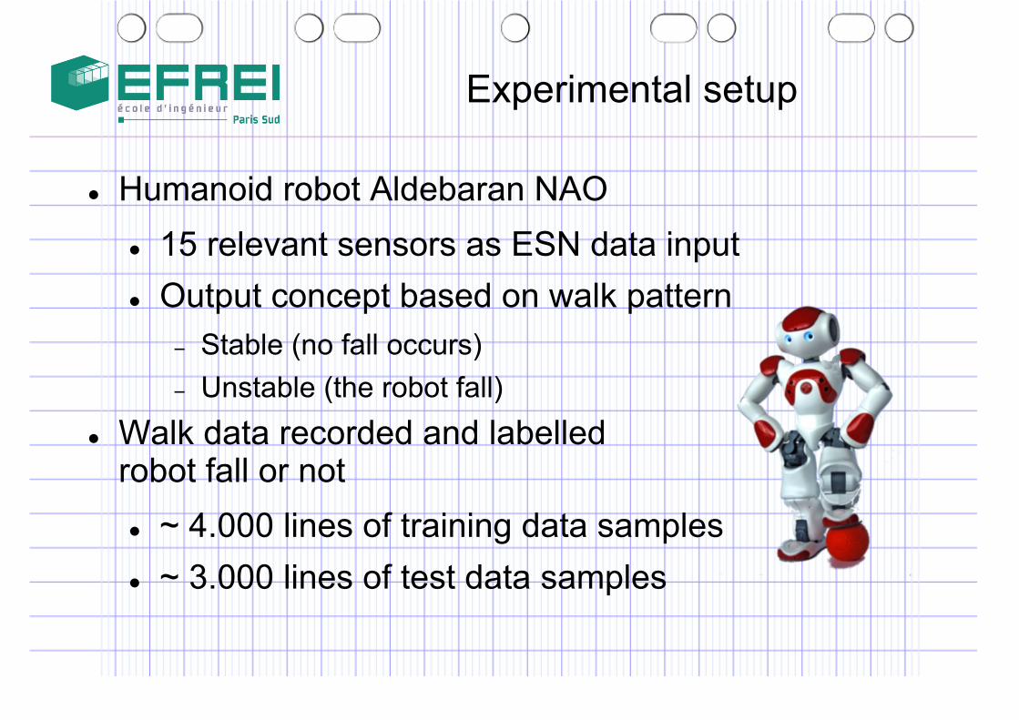
Experimental setup
Humanoid robot Aldebaran NAO 15 relevant sensors as ESN data input Output concept based on walk pattern
− Stable (no fall occurs)− Unstable (the robot fall)
Walk data recorded and labelledrobot fall or not ~ 4.000 lines of training data samples ~ 3.000 lines of test data samples
Page 14
Parameters
ESN parameters (inputs,reservoir, outputs) = (15, 100, 1) Damping = 0.9 Connection density = 0.1 Activation function = Hyperbolic Tangent
Evolution Parameters Covariance Matrix Adaptation (CMA-ES) [Hansen 05]
meta-optimisation involving no parameters Fitness F = (1/N) ∑ [y(i) – d(i)]2
Page 15
Results
Over 16 walk samples, up to 4000 points plotted.
0 value indicates a no movement stable state of the robot, +0.5is a stable walk and -0.5 indicates instability leading to fall.
Page 16
3 Different Test Fall Patterns
Page 17
Discussion
For stable samples ESN provides negative output atvery few points.
For the fall samples, ESN does not immediatelyclassify a data as ”Fall”.
The output value does not jump directly from +0.5 to -0.5. Enables to predict a fall in advance and we havealmost half a second to initiate an action
Unstable points in stable pattern and stable walkbefore a fall proves the concurrency with practicalobservation.
Page 18
Conclusion
Reservoir Computing as meta-sensors Not used for control but as middleware between
sensors and control architecture Echo State Networks based approach First validation over Fall detection
− Able to predict fall on short term− Able to detect unstable walks
Perspectives Compare to Liquid State Machines and NEAT Train to predict on longer terms