POUR L'OBTENTION DU GRADE DE DOCTEUR ÈS SCIENCES acceptée sur proposition du jury: Prof. P. Monkewitz, président du jury Prof. J. R. Thome, directeur de thèse Prof. J. Bonjour, rapporteur Prof. D. Favrat, rapporteur Prof. G. Ribatski, rapporteur Falling Film Evaporation on a Tube Bundle with Plain and Enhanced Tubes THÈSE N O 4341 (2009) ÉCOLE POLYTECHNIQUE FÉDÉRALE DE LAUSANNE PRÉSENTÉE LE 3 AVRIL 2009 À LA FACULTÉ SCIENCES ET TECHNIQUES DE L'INGÉNIEUR LABORATOIRE DE TRANSFERT DE CHALEUR ET DE MASSE PROGRAMME DOCTORAL EN ENERGIE Suisse 2009 PAR Mathieu HABERT
Transcript
POUR L'OBTENTION DU GRADE DE DOCTEUR ÈS SCIENCES
acceptée sur proposition du jury:
Prof. P. Monkewitz, président du juryProf. J. R. Thome, directeur de thèse
Prof. J. Bonjour, rapporteur Prof. D. Favrat, rapporteur
Prof. G. Ribatski, rapporteur
Falling Film Evaporation on a Tube Bundle with Plain and Enhanced Tubes
THÈSE NO 4341 (2009)
ÉCOLE POLYTECHNIQUE FÉDÉRALE DE LAUSANNE
PRÉSENTÉE LE 3 AvRIL 2009
À LA FACULTÉ SCIENCES ET TECHNIQUES DE L'INGÉNIEUR
LABORATOIRE DE TRANSFERT DE CHALEUR ET DE MASSE
PROGRAMME DOCTORAL EN ENERGIE
Suisse2009
PAR
Mathieu HABERT
Abstract
The complexities of two-phase flow and evaporation on a tube bundle present importantproblems in the design of heat exchangers and the understanding of the physical phenom-ena taking place. The development of structured surfaces to enhance boiling heat transferand thus reduce the size of evaporators adds another level of complexity to the modelingof such heat exchangers. Horizontal falling film evaporators have the potential to bewidely used in large refrigeration systems and heat pumps, in the petrochemical industryand for sea water desalination units, but there is a need to improve the understandingof falling film evaporation mechanisms to provide accurate thermal design methods. Thecharacterization of the effect of enhanced surfaces on the boiling phenomena occurringin falling film evaporators is thus expected to increase and optimize the performance ofa tube bundle. In this work, the existing LTCM falling film facility was modified andinstrumented to perform falling film evaporation measurements on single tube row anda small tube bundle. Four types of tubes were tested including: a plain tube, an en-hanced condensing tube (Gewa-C+LW) and two enhanced boiling tubes (Turbo-EDE2and Gewa-B4) to extend the existing database. The current investigation includes resultsfor two refrigerants, R134a and R236fa, at a saturation temperature of Tsat = 5◦C, liquidfilm Reynolds numbers ranging from 0 to 3000, at heat fluxes between 20 and 60kW/m2
in pool boiling and falling film configurations. Measurements of the local heat transfercoefficient were obtained and utilized to improve the current prediction methods. Finally,the understanding of the physical phenomena governing the falling film evaporation ofliquid refrigerants has been improved. Furthermore, a method for predicting the onsetof dry patch formation has been developed and a local heat transfer prediction methodfor falling film evaporation based on a large experimental database has been proposed.These represent significant improvements for the design of falling film evaporators.
Keywords: falling film evaporation, pool boiling, enhanced boiling, heat transfer, two-phase flow, Wilson plot
iv Abstract
Version Abrégée
La complexité des écoulements diphasiques au sein d’un faisceau de tubes soulève de nom-breux problèmes de compréhension des phénomènes physiques y prenant place et, par lasuite, lors de leur dimensionnement. Le développement récent de surfaces améliorées cen-sées améliorer le transfert de chaleur, et donc, réduire la taille de l’évaporateur, rajouteun autre degré de complexité lors la modélisation de ces échangeurs de chaleur. Les éva-porateurs à film tombant ont le potentiel pour être largement utilisés pour des grandesunités frigorifiques dans des pompes à chaleur et dans l’industrie pétrochimique ou pourle dessalement de l’eau de mer, mais il est nécessaire d’améliorer au préalable la connais-sance des mécanismes d’évaporation en film pour fournir des méthodes performantes dedimensionnement pour échangeurs de chaleur. La caractérisation de l’influence des sur-faces améliorées sur le phénomène d’ébullition se produisant dans les évaporateurs à filmtombant devrait permettre de mieux comprendre l’augmentation et d’optimisation desperformances observées avec un faisceau de tubes. Par conséquent, l’installation expéri-mentale du LTCM pour les échanges en film tombant a été modifiée avec l’instrumentationnécessaire pour effectuer des mesures sur une colonne de tubes horizontaux et un petit fais-ceau de tubes. Quatre types de tubes ont été testés: un tube lisse, un tube amélioré pourla condensation (Gewa-C+LW) et deux tubes améliorés pour l’ébullition (Turbo-EDE2 etGewa-B4) afin d’augmenter la base de données existante. L’étude suivante présente desrésultats obtenus avec deux réfrigérants, R134a et R236fa, une température de saturationTsat = 5◦C, des nombres de Reynolds compris entre 0 et 3000, des densités de flux dechaleur entre 20 et 60kW/m2 (méthode de Wilson, ébullition en vase et évaporation enfilm tombant). Des mesures locales du coefficient de transfert de chaleur ont été obtenueset utilisées pour améliorer les méthodes actuelles de prédiction. A l’issue de ce travail,la compréhension des phénomènes physiques régissant l’évaporation des réfrigérants enfilm tombant a été améliorée. Deux méthodes ont été proposées: une pour la prédic-tion de l’apparition de la formation de zones sèches et une pour le transfert de chaleurde l’évaporation en film tombant, basée sur une grande base de données expérimentales.Elles constituent une amélioration significative pour la conception des évaporateurs à filmtombant.
Mots clés: évaporation en film tombant, ébullition en vase, ébullition améliorée, transfertde chaleur, écoulement biphasique, méthode de Wilson
vi Version Abrégée
Acknowledgments
This study has been carried out at the Laboratory of Heat and Mass Transfer (LTCM),Swiss Federal Institute of Technology Lausanne (EPFL), under the direction of Prof.John R. Thome. This project has been supported financially by the LTCM Falling FilmResearch Club members: Johnson Controls Inc., Trane, Wieland-Werke AG and Wolver-ine Tube Inc, which is gratefully acknowledged. Special acknowledgment is made toWieland-Werke AG and Wolverine Tube Inc for providing the tube samples for the tests.
I would like to thank Prof. John R. Thome for giving me the opportunity to perform thisinvestigation in his laboratory. His experience and expertise in two-phase flow guided meover the past years. I also would like to express my gratitude to my thesis examiners,Prof. Jocelyn Bonjour, INSA Lyon, Prof. Daniel Favrat, EPFL and Prof. GherhardtRibatski, Universidade de São Paulo.
I would like to thank also all my colleagues of the LTCM, who contributed in differentways to this thesis, with warm coffee breaks and interesting discussions over the lastyears. I particularly thank Laurent Chevalley for helping me with the technical work andmaking me discover Switzerland and its beauties.
Finally, I would like to thank all my friends and family for their support, and particularlySarifa, my future wife, who hopefully will support me for all my life.
Csf constant in Rohsenow correlation Eq. (2.23) [-]
D tube diameter [m]
db bubble diameter [m]
dd droplet diameter [m]
F apparent wet area fraction [-]
f friction factor [-]
fb bubble frequency [Hz]
g gravitational acceleration [g = 9.81m/s2]
H enthalpy [J/kg]
h local heat transfer coefficient [W/m2K]
HLV latent heat of vaporization [J/kg]
k thermal conductivity [W/mK]
Kff falling film multiplier [−]
L characteristic length [m]
Ld developing length [m]
m mass flow [kg/s]
M molar mass [kg/kmol]
N number of nucleation sites [−]
xix
xx Nomenclature
P tube pitch [m]
pr reduced pressure [−]
q local heat flux [W/m2]
rcav cavity radius [m]
Rp peak roughness [m]
rwall tube wall thermal resistance [K/W ]
Rwall tube wall thermal resistance [m2K/W ]
T temperature [K]
U overall heat transfer coefficient [W/m2K]
ug vapor crossflow velocity [m/s]
Greek Symbols
α thermal diffusivity [m2/s]
β volumetric thermal expansion coefficient [1/K]
Γ liquid film flow rate on one side of the tube per unit length [kg/ms]
λ wavelength [m]
µ dynamic viscosity [Pa.s]
ν kinematic viscosity [m2/s]
ρ density [kg/m3]
σ surface tension [N/m]
φ angle [rad]
θ critical angle [rad]
Subscripts
b boiling
c convective
crit critical
D dangerous
d developing
gni Gnielinski
Nomenclature xxi
h hydraulic (diameter)
i internal side
imp impingement
L saturated liquid
o external side
pb pool boiling
r (fin) root
ref refrigerant
sat saturation conditions
V saturated vapor
wat water
Dimensionless Numbers
Bo Bond number, Bo = g(ρL − ρV )D2/σ
Ga modified Galileo number, Ga = ρLσ3/µ4
Lg
Nu Nusselt number, Nu = hD/k
Pr Prandtl number, Pr = Cpµ/k
Ra Rayleigh number, Ra = gβ(T − T∞)D3/να
Re Reynolds number, Re = 4Γ/µ
We Weber number, We = ρσ3/µ4g
xxii Nomenclature
Chapter 1
Introduction
The environmental issues of ozone depletion and global warming have considerably af-fected the refrigeration, air-conditioning and heat pump industry over the last 10 years.The introduction of non chlorine-containing refrigerants and the development of new heattransfer concepts are necessary to achieve the goals of reduced energy consumption andenvironmental impact.
Shell and tube heat exchangers are widely used in the refrigeration industry, particularlyfor evaporators in large capacity units. In flooded evaporators, liquid refrigerant entersthe evaporator from the bottom and evaporates as it moves up the tube bundle due tothe buoyancy of the vapor. On the other hand, falling film evaporators are based on aheat transfer process that takes place when the refrigerant is flowing downwards, due togravity, on the heated tube bundle. Applied to a refrigeration system, the falling filmevaporator presents several advantages compared to a flooded evaporator, particularly interms of higher cycle efficiency, reduced costs and a smaller environmental impact fromits reduced charge of refrigerant. The pressure drop is small as the liquid flows onlyby gravity, which may imply the use of a recirculation pump to bring the liquid fromthe bottom to the top of evaporator. There are many parameters influencing the fallingfilm evaporation process and, despite numerous studies, the basic mechanisms remainunclear, making the prediction approach mainly empirical. The main design parametersto correlate are the onset of dryout that can degrade the evaporator performance, andthe heat transfer coefficient whose evolution can help to optimize the evaporator.
Bergles [1] documented the number of journal publications related to heat transfer en-hancement technology over the years showing a rapid growth until the 1990s. Surfaceenhancement technology in recent years has been highly focused on the improvement oftwo-phase heat transfer with mechanically fabricated enhanced surfaces, thus providinghigh nucleation site density to trap vapor and optimize bubble generation. As under-lined by Thome [2], the key fundamental problems regarding the physical processes andphenomena remain unsolved and investigators need to collect a large database to try todeduce how the structure of the surface affects the heat transfer performance.
The aim of the present investigation is to collect experimental data on falling film evap-oration with plain and enhanced surfaces to better understand the mechanisms linkedto two-phase flow and evaporation on a dense array of tubes in heat exchangers. The
2 Introduction
LTCM falling film facility was designed and built in the previous studies of Roques [3]and Gstoehl [4]. Numerous results on a single-array (one row) were obtained with differ-ent heat fluxes and tube pitches. This study provides extensive new information on thebehavior of structured surface for two different fluids; the facility was adapted for fallingfilm heat transfer measurement in tube bundle (3-rows of 10 tubes each in the array). Lo-cal heat transfer coefficients were measured in single-array and in bundle configuration toobtain new heat transfer data. The new results were then used to develop new predictionmethods for two-phase heat transfer and a new onset of dryout prediction method.
The thesis is organized as follow:
• Chapter 1: Introduction
• Chapter 2: State of the art review on falling film heat transfer
• Chapter 3: Description of the test facility modifications and instrumentation
• Chapter 4: Description of the data processing and measurement uncertainties
• Chapter 5: Analysis of the local heat transfer coefficients obtained in a single-rowfor plain and enhanced tubes
• Chapter 6: Presentation and discussion of the experimental results obtained for thetube bundle
• Chapter 7: Predictions methods for the onset of dryout and the local heat transfercoefficient in single-row and for the tube bundle
• Chapter 8: The conclusions of this study are summarized
Chapter 2
State of the art review
2.1 Hydrodynamics of a liquid film
According to a comprehensive state of the art review on falling film evaporation on hori-zontal tubes presented by Ribatski and Jacobi [5], the thermal performance of the falling-film heat exchanger may be drastically affected by the distribution of the fluid refrigerantalong a tube bundle according to the following aspects:
• type of flow mode between adjacent surfaces,
• unsteadiness of the flow,
• film thickness along the heating surfaces,
• flow contraction along the tube bundle,
• spacing of droplet and column departure sites,
• “slinging” effect [6],
• film breakdown and hot patches.
The sections below discuss the status of some of these topics.
2.1.1 Falling film intertube modes and transitions
Instability mechanisms play important roles in falling film evaporation. Liquid film flowsare usually dominated by viscous, gravity and surface tension effects. Circumstancesmay give rise to interfacial waves on the thin liquid film that may strongly affect thevaporization rate by increasing the interfacial area and enhancing convective transportnear the interface.
When a liquid film flows from one horizontal tube to another below it, the flow may takethe form of droplets, circular columns, or a continuous sheet. The droplet, column and
4 State of the art review
sheet mode represent the principal flow modes. Droplet-column and column-sheet, thatis, flow modes between the principal ones, have also been identified. A distinction is alsomade for the column mode according to the relative positions of the columns impingingand departing onto the top and from the bottom of the tube, respectively. The in-linecolumn mode is defined when the columns are vertically aligned at the top and bottom.The staggered column is defined as that when the columns’ positions are shifted fromone intertube space to the following one, one-half λ out of phase. The thickness of aliquid film on the horizontal tube varies around the tube periphery since the gravity forcecomponent in the flow direction varies around the perimeter. Presently, circumferentiallyaveraged heat transfer coefficient around the perimeter of the tube are considered in thisstudy and can be termed to be “axially local” along the tube.
In a horizontal falling-film evaporator, the physical form of the liquid film depends notonly on the liquid flowrate leaving the tube but also on the distance between the tubesas described by Jung et al. [7]. When the flowrate is small and the tube spacing large,the liquid flow is usually in a form of droplets at discrete points along the underside ofthe tube.
Figure 2.1: Intertube falling-film modes: (a) droplet mode; (b) column mode; (c) sheet mode;(d) illustration of the Taylor instability [8]
For the droplet and column flow modes, liquid usually falls from fixed sites along theunderside of the tube. Fig. (2.1) shows some details of how the liquid film is formed. Fromthe stagnation point of an oncoming column, the liquid flows along the tube in both axialdirections. In the region when the spreading streams from the two columns overlap, aliquid crest is formed. The crest flows around the perimeter of the tube like a ring and thedistance between them is related to the Taylor instability. For circumstances in which
2.1. Hydrodynamics of a liquid film 5
viscous effects are negligible and the fluid is incompressible, Bellman and Pennington[9] found that the critical wavelength and most dangerous Taylor wavelength are givenrespectively by:
λcrit = 2π√
σ
g(ρL − ρV ) (2.1)
λD = λcrit√
3 (2.2)
Only perturbations having wavelengths between λc and λD will grow. However, λD is thewavelength for which the disturbance grows most rapidly. Therefore, in real systems, thedominant disturbance wavelength is generally close to λD. Mitrovic [10] found departure-site spacing between the critical and the most dangerous wavelength, whereas Yung etal. [7], performing an experimental study with water, ethylene glycol and ammonia, con-cluded that λ is given by λc
√2. Similar methods were developed by other authors, but
Eq. (2.1) and Eq. (2.2) give good agreement based on simple expressions.
Flow modes of a liquid film falling on an vertical array of tubes depend principally onthe flow rate and the physical properties of the liquid. Extensive studies focusing on thecharacterization and prediction of falling film intertube flow modes were performed byHu and Jacobi [11] and, Armbruster and Mitrovic [12], on plain tubes, and recently byRoques et al. [13] on plain and enhanced tubes. Prediction methods for flow transitionswere first proposed by Honda et al. [14] on a low finned tube and, recently, by Hu andJacobi [11] on plain tubes and by Roques et al. [13] on plain and enhanced tubes, all foradiabatic conditions. Flow mode transitions were correlated as follows:
Re = aGab (2.3)
where the film Reynolds number and the modified Galileo number are defined as
Re = 4Γµ
(2.4)
Ga = ρLσ3
µ4Lg
(2.5)
Comparing the current prediction methods for flow mode transitions, Ribatski and Jacobi[5] found a significant scatter among them, which is reasonable given the subjective natureof interpreting two-phase flow regime transitions.
The flow mode may be an important parameter in the optimization of falling film heatexchangers. The sheet mode seems to be the most convenient flow modes for falling filmevaporation. This mode will best avoid the formation of dry patches on the heat transfersurface, although this may result in a waste of energy for pumping the excess liquid backto the distributor.
The effect of flow mode on the heat transfer performance will be discussed later.
6 State of the art review
2.1.2 Film breakdown and hot patches
If the flow rate of the liquid film is reduced sufficiently or if the amount of heat added tothe surface is relatively high, the film will thin, break down and dry patches will appear.These dry patches on the tube surface result in a steep decrease in the heat transfercoefficient. A schematic of falling film breakdown is given in Fig. (2.2).
Figure 2.2: Schematic of a stable dry patch [15]
As described by Ganic et al. [16], the mechanisms and fluid forces involved in dry patchformation and its evolution are:
• the inertial force: the upstream liquid decelerates at the stagnation point whichfavors the rewetting of dry patches,
• the surface tension force: due to a nonzero contact angle between the liquid andsolid surface, this helps to increase the dry patch size,
• the thermocapillary force (also called the Marangoni effect): a force resulting fromthe variation of surface tension due to the temperature gradient on the surfacetends to transport liquid away from the thinnest location in the layer, inducing drypatches to form,
• the vapor thrust: the vapor creates a suction force around the liquid film whichtends to enlarge the size of the dry patch,
• the interfacial shear force: the vapor entrains the liquid leading edge and tends tothin the liquid film, particularly for upward vapor flow.
In reality, the breakdown of a liquid film on a smooth heated tube appears to be mainlycontrolled by the surface tension phenomenon. A variation in film thickness due to wavesleads to variation in the surface temperature. The thinner parts of the film (valleys)reach a higher interfacial temperature causing an even larger local variation of surface
2.1. Hydrodynamics of a liquid film 7
tension. The liquid will be drawn from the thin region of the film to the thicker parts(crests) and eventually local dry patches will appear on the surface when increasing theheat flux. These dry patches are usually observed beneath a crest at the lower part of thetube array. Ganic et al. [16] observed that some dry patches were not stable, sometimesre-wetting themselves.
Figure 2.3: Schematic of liquid film breakdown from [8]
Fig. (2.3) from Thome [8] shows the observed liquid flow on a row of tubes for two differentfilm flow rates, including flow contraction and intertube flow modes. This flow contractionwas also observed and described by Fujita et al. [17]. They investigated breakdown offalling films with R-11 on plain tubes and defined a wetted area fraction ζ as a functionof the heat flux, flow rate and tube location.
2.1.3 Vapor/liquid interaction
Compared to the intube vertical tube falling film configuration favored by the petrochem-ical industry, horizontal falling film evaporator design is considerably more vulnerable tovapor/liquid interaction. Reliable evaporator design requires a clear understanding of theeffect of vapor crossflow. As a result of vapor crossflow, the droplets and columns fallingfrom one tube may be partially or totally deflected away from the next tube, causing
8 State of the art review
liquid redistribution and incomplete wetting of lower tubes with liquid leaving the arraysideways. Entrainment mechanisms can also occur, as described by Yung et al. [7]:
• if nucleate boiling is present in the film, a mist of small droplets is generated asbubbles burst through the film and these small droplets are entrained in the flowingvapor,
• shearing or “stripping” of the liquid film from the tube surface,
• deflection of droplet/column due to the growth of instability waves for high vaporvelocity as depicted in Fig. (2.4),
• liquid splashing depending of wettability and fluid velocity.
Figure 2.4: a) Droplet deflection due to vapor cross flow b) Column deflection due to vaporcrossflow [7]
Yung and Lorenz [7] defined a critical angle θdroplet beyond which the droplet will not hitthe lower tube (see Eq. (2.6)). Based on the pitch-to-diameter ratio P/D and the criticaldeflection angle θcolumn (see Eq. (2.7)), they solved the equations of motion of a singledroplet to obtain the following two expressions:
θdroplet = tan−1(
12
[P
D
(P
D− 1
)]−1/2)(2.6)
θcolumn = tan−1[13ρgρl
u2g
dd
](2.7)
From Eq. (2.7) and Eq. (2.6), they obtained the maximum allowable vapor crossflowvelocity ug.
2.2. Heat transfer mechanisms 9
ug =(
32ρlρgdd
)1/2 [P
D
(P
D− 1
)]−1/4(2.8)
They also conducted a similar but more complex analysis for the liquid column deflection,available in the cited article. They underlined the fact that this deflection of liquid doesnot necessary imply a loss of heat transfer performance, because the liquid may experiencea good “hit”. In essence, good wetting on the tube is essential to ensure a good heattransfer performance and a well-controlled liquid flow is preferable to relying on randomliquid hits on tubes in adjacent columns.
2.1.4 Tube bundle flow
With the formation of a horizontal gravitational liquid film on the surface of a horizontalcircular tube, a non-stabilized flow practically always results since the main driving forceis a projection of the gravitational force on the surface of the tube, which varies aroundthe perimeter. This induces acceleration of the film on the upper part of the tube anddeceleration on the lower part and in a such way it introduces momentum forces not ac-counted for in Nüsselt’s classic theory [18]. Additionally, momentum forces appear due toliquid impingement on the top of the tube and its run off. The hydrodynamic processesbecome more complicated for wavy or turbulent film flow on a vertical row of horizon-tal tubes with strongly developed vortex formation in the intertube spacing. For smallintertube spacing, the surface tension forces will increase pressure 90◦ from the impinge-ment area and decrease it in the intertube spacing, having a particular effect on the filmthickness as described by Sinkunas [19]. Surface tension plays a significant role. Evenwhen formally small, surface tension often has a significant smoothing effect preventingthe formation of shocks (sharp jumps in the film thickness). Generally speaking, surfacetension effects tend to flatten a film (to reduce curvature), thus producing a smooth film.This beneficial effect is limited where curvature variation is small [20].
The interfacial drag on the liquid film in a tube bundle is determined by the flow patternin the space between the tubes. Significant accelerations and decelerations of the flow,characteristic to tube bundles, induce a drag effect on the flow. Consequently, the tubegeometry and layout affect the drag. At low Reynolds numbers, the drag is represented byviscous friction and is directly proportional to the velocity. When the Reynolds numberis increased, eddies are generated and cause a loss of kinetic energy in addition to theviscous friction, coupling the relationship between the velocity and the drag.
2.2 Heat transfer mechanisms
The hydrodynamic behavior of a fully developed isothermal falling film is retained alsowhen heat transfer is superimposed on the flow, as long as film breakdown does not occur.For Rohsenow [21], the resistance to heat transfer resides in a thin thermal layer adjacentto the wall which is approximately equal to the residual film thickness. According tohim, outside this thermal boundary layer, the mixing action of the interfacial waves
10 State of the art review
leads to approximately a constant film temperature. For the case of saturated fallingfilms, convective heat transfer leads to evaporation at the liquid-vapor interface. With anincrease of heat flux, nucleate boiling occurs. It was reported that boiling occurs first onthe lower side of the tube, near the downstream stagnation point. Vapor bubbles growand are carried along by the film flow. Both thin falling film evaporation and nucleateboiling play a role in the heat transfer process, depending mainly on the heat flux andliquid mass flow rate.
Chyu and Bergles [22] defined three heat transfer regions illustrated on Fig. (2.5): the jetimpingement region, the thermally developing region and the fully developed region.
Figure 2.5: Falling film thermal regimes
The jet impingement region is a short region in which the heat transfer coefficient isrelatively high due to liquid feed at the top of the tube. In the thermally developing region,the film is superheated from the uniform saturation temperature to a fully developedprofile; all the heat transferred from the wall goes to superheating the liquid film andno evaporation occurs. In the fully developed region, all of the heat transfer goes toevaporation at the liquid/vapor interface if no nucleate boiling occurs within the film.
The convective and boiling heat transfer regimes have to be considered separately becausethe two heat transfer mechanisms are different.
2.2.1 Convection
Natural convection within the heat exchanger is due to local density gradients withinthe heat exchanger. At low flow rates these natural convection effects become evident.Although the liquid refrigerant is being propelled downward by gravity, some of the vapor
2.2. Heat transfer mechanisms 11
in the heat exchanger moves on its own due to localized natural convection. When thetubes are hot, the vapor that comes close to the tubes is heated, becomes less dense, anddisplaces the nearby vapor that does not come into contact with the copper tubes. Inthis case, flow can be characterized as a combination of forced and natural convection.
Morgan [23], Churchill and Chu [24] and others have determined empirical correlationequations which focus mainly on the area and time-averaged Nüsselt number for naturalconvection. For an isothermal cylinder, Morgan proposed the following equation:
Nu = hD
kL= CRan (2.9)
For tabulated values of C and n, refer to [23]. Churchill and Chu recommended a singlecorrelation for a wide range of Rayleigh numbers:
Nu =(
0.60 + 0.387Ra1/6
[1 + (0.559/Pr)9/16]8/27
)2
(2.10)
This equation is valid for Ra ≤ 1012 and is probably the most widely used for naturalconvection.
2.2.2 Nucleate pool boiling
The Rohsenow [25] correlation, to predict the heat transfer coefficient in nucleate poolboiling, was among the first to be recognized. According to Rohsenow, the high heattransfer rates associated to nucleate pool boiling are caused by bubbles departing fromthe surface. The resulting correlation has the following form:
Nub = hD
kL= 1Csl
Re(1−n)Pr−ml (2.11)
Csl as well as m and n are constants depending on different nucleation properties of aparticular liquid/surface combination, while the Reynolds number was expressed usingthe superficial liquid velocity on the surface:
Re = q
Hlvρl
[σ
g(ρl − ρv)
]1/2ρlρv
(2.12)
Ishibashi [26] proposed a fairly simple correlation between heat flux and heat transfercoefficient for boiling of saturated water in narrow spaces in the form of
h ∝ qn (2.13)
Stephan [27] recommended values of around 0.6 to 0.7 for n. In a previous study, Stephanet al. [28] proposed a correlation for several fluids including water, organics, refrigerantsand cryogens:
12 State of the art review
h = 207 kldb
[qdbklTsat
]0.745 [ρvρl
]0.581
Pr0.533l (2.14)
In this correlation, the bubble diameter db was calculated according to Fritz [29]:
db = 1.192φcontact√
σ
g(ρl − ρv)(2.15)
Cooper [30] correlated the heat transfer coefficient with not only heat flux, but alsoreduced pressure, surface roughness and molecular weight. For boiling on horizontalplane surfaces, the heat transfer coefficient is given by:
h = 55Cp0.12−0.2log10Rpr (−log10pr)−0.55M−0.5q0.67 (2.16)
For boiling on horizontal copper cylinders, the constant C has to be chosen equal to 1.7.This correlation is probably the most widely used to accurately predict nucleate poolboiling heat transfer coefficients. It is valid for 0.001 ≤ pr ≤ 0.9 and 2 ≤M ≤ 200.
Gorenflo [31] developed a method for predicting nucleate pool boiling coefficients us-ing a reference heat transfer coefficient h0 obtained at reference conditions (pr0 = 0.1,Rp0 = 0.4µm and q0 = 20000W/m2). Knowing h0, the heat transfer coefficient at otherconditions is given by:
h = h0FPF
(q
q0
)nf (Rp
Rp0
)0.133
(2.17)
The pressure correction factor FPF was obtained by:
FPF = 1.2p0.27r + 2.5pr + pr
1− pr(2.18)
and the index nf was given by:
nf = 0.9− 0.3p0.3r (2.19)
Boiling in a thin liquid film differs from its pool boiling counterpart. Falling film evap-oration provides much higher heat transfer coefficients than pool boiling in the low heatflux, convective region. Cerza and Cernas [32] hypothesized that the enhancement toheat transfer from nucleate boiling in the liquid film is due to the fact that a bubble liesembedded in the superheated liquid film, compared to nucleate boiling where the bubblegrowth is generally confined to the thickness of the superheated thermal layer next to thewall.
2.3. Falling film enhancement 13
2.3 Falling film enhancement
Numerous attempts have been made to improve the heat transfer performance by us-ing enhanced surfaces. A great variety of enhancement techniques have been developedand applied to horizontal falling film evaporators: structured surfaces (porous metallicsurfaces, knurled tubes), rough surfaces (ribbed or grooved tubes), extended surfaces(circumferential or helical fins)...
The general objective of these techniques is to reduce the size of the evaporator and in-crease the heat transfer efficiency by reducing the driving temperature difference. Typi-cally, enhanced surfaces on the outside of tubes are for enhancing nucleate boiling, whereasthose on the inside are for enhancing the heat transfer from the chiller water flowing inside.Refer to Bergles [33] and Thome [2] for comprehensive treatments of this subject.
Figure 2.6: Evaporation processes on an enhanced boiling surface, from Thome [2]
The enhanced boiling process is different from normal nucleate boiling from cavities.Evaporation occurs both on the external surface and inside its reentrant channels. Thus,there are four possible ways for heat to be dissipated, as illustrated in Fig. (2.6):
1. As latent heat generating vapor within the reentrant channels,
2. As latent heat into bubbles growing on the outside surface of the enhancement,
3. As sensible heat to the liquid “pumped” through the reentrant channels and backout,
4. As sensible heat to the liquid in the external thermal boundary layer.
If enhanced surfaces were originally developed to improve nucleate pool boiling, they haveonly been applied to thin film evaporation since the 1980s. Structured surfaces promotenucleate boiling in the film at modest temperature differences, enhance turbulence withinthe film, and provide an increase in heat transfer area.
14 State of the art review
The parameters influencing the degree of enhancement are mainly the shape, geometryand surface area of the cavities and the nucleation site density while for porous coatingson surfaces the principal parameters are the particle size, the coating thickness and theporosity. Using the equation of Laplace and Clasius-Clapeyron, it can be shown that thewall superheat required for a bubble to exist at the mouth of a cavity of radius rcav isgiven by:
Twall − Tsat = qrcavkL
+ 2σLTsatρVHLV rcav
(2.20)
The bubble departure diameter db can be calculated assuming the buoyancy force equalsthe surface tension force at the time of departure. The force balance gives:
db = Cb
[2σ
(ρL − ρV )g
](2.21)
The nucleation site density N/A was correlated by different authors as proportional tothe heat transfer coefficient: h ∝ (N/A)n. Chien and Webb [34], [35] investigated theeffect of pore diameter, pore pitch and tunnel shape using R11 and R123. They foundthere is a preferred pore diameter and pore pitch for a specific heat flux range. The mainproblem here is that the determination of the above parameters is extremely difficult andis purely empirical.
The behavior of structured surfaces is not well understood. As such, the point has notyet been reached where reliable methods are available to guide the custom design of theenhanced surface geometry for a particular fluid and operating condition. Poniewski andThome [36] have recently proposed a new, free web book dedicated to the state-of-the-artof this topic.
2.4 Single tube and single tube row heat transferstudies
Falling film evaporation has been widely studied in terms of effects such as liquid feed flowrate, liquid distribution method, liquid feed flow pattern, liquid feed temperature, tubesurface structure, surface aging, tube spacing, heat flux, surface subcooling, vapor crossflow, etc. Experimental data for boiling of thin films is relatively scarce when compared tothe abundance of data for pool boiling. Much of the previous studies were made for OceanThermal Energy Conversion (OTEC) and desalination research on water. Unfortunately,only a few data are available for other working fluids, such as refrigerants.
2.4.1 Saturation temperature effect
In the convective evaporation regime (without nucleate boiling), authors like Fletcher etal. [37], Parken et al. [38] or Armbruster et al. [39] observed an increase of performance
2.4. Single tube and single tube row heat transfer studies 15
with increasing saturation pressure. This increase is related to the variation of viscositywith temperature and consequently to the film thickness. For the boiling regime, theeffect of saturation temperature is not so clear. Zeng et al. [40] pointed out an increasein heat transfer coefficient, whereas Parken et al. [38] observed an opposite behavior forcertain conditions. According to Ribatski and Jacobi [5], two competing effects can eitherincrease or decrease the heat transfer coefficient: an increase of the activated nucleationsite density with temperature and bubble growth inhibition due to a steeper temperatureprofile.
2.4.2 Heat flux effect
The effect of heat flux for the convective evaporation region was found to not affect theheat transfer performance by several authors like Fujita et al. [41] and Hu and Jacobi [42].On the other hand, for nucleate boiling-dominated conditions, higher heat transfer coeffi-cients are obtained for higher heat flux because of an increased nucleation site density asdescribed by Moeykens [43] and Zeng et al. [40]. The variation of heat transfer coefficientwith heat flux has been noted as particularly high for low reduced pressure fluids byFletcher et al. [44].
2.4.3 Flow rate effect
Under stricly-convective evaporation conditions, two different behaviors were described inthe literature: an increase of heat transfer performance with increasing flow rate as foundby Ganic and Roppo [45] and non-dependence on the flow rate. For nucleate boiling-dominated conditions, the heat transfer coefficient becomes independent of the flow rateas noted by Chyu and Bergles [46] and Moeykens and Pate [43]. Roques [3]
proposed another heat transfer measurement strategy to obtain the local value at themidpoint of each tube, using a modified Wilson plot technique combined with measure-ment of the heating water temperature profile. According to him, the trend for fallingfilm evaporation is made up of two distinct regions as shown on Fig. (2.7): a plateaucorresponding to an all-wet nucleate boiling-dominated regime where the heat transfercoefficient varies little with the flow rate, a point of onset of dryout, and a partially-wetregime with nucleate boiling in the remaining film with a thus rapidly decreasing heattransfer coefficient tending towards the vapor phase natural convection coefficient at com-plete dryout. Hence, the onset of dryout is an important part of the heat transfer processand its modeling. Instead, once through hot water heating with tube-length averagedheat transfer coefficients with progressive dryout from one end to the other tend to givethe monotonic trend illustrated in Fig. (2.7).
2.4.4 Tube diameter effect
The effect of tube diameter is related to the thermal boundary layer development andimpingement region length relative to the “unwrapped” length πD/2. For non-boiling
16 State of the art review
Figure 2.7: Schematic of the variation of heat transfer coefficient with flow rate for falling filmevaporation
conditions, Parken and Fletcher [47] measured a higher heat transfer coefficient for smallertube diameters. The respective proportion of the impingement region on the overall flowarea increases with decreasing diameter giving higher performance. Such a noticeablediameter effect is not expected when nucleate boiling is dominant.
2.4.5 Liquid feeder effect
The configuration and the height of the liquid feeder above the top of the tube can affectthe evaporator performance. A poorly designed or mal-situated feeder will cause a non-uniform axial uniformity of the liquid film and can lead to refrigerant maldistributionand premature formation of dry patches. Different liquid feeders were tested in theliterature, such as perforated plates or spray nozzles, and the influence of their height onthe impinging effect was studied.
Fletcher et al. [44] used a perforated plate instrumented with thermocouples at 3 locationsaround the tube to see the possible variation of circumferential temperature. They notedan axial temperature variation due to flow non-uniformity. Fujita and Tsutsui [48], [41]compared the heat transfer performance obtained for 3 different feeders: a sintered poroustube, a tube with nozzles and a plate with nozzles. They found that the porous sinteredtube and the perforated plate with one, two or three dummy tubes performed 20% betterthan the cylindrical feeder with holes along the top. For Chyu et al. [49], the liquidflow rate given by nozzles depended on spray angle, nozzle height, nozzle interval, tubediameter, spray coverage and distribution of the liquid droplet within the spray coveragearea. They analyzed different nozzle configurations to look at the spray coverage and theuniformity of the distribution. Moeykens and Pate [43] reported results for wide-anglelow- and high-pressure-drop nozzles. The high-pressure-drop nozzles gave the best perfor-mance, probably because of a higher impingement effect. An increase of the feeder heightresulted in higher impingement velocities which influenced the performance of the toptubes. It may also yield better uniformity of the spray and thus mitigate maldistributioneffects.
2.4. Single tube and single tube row heat transfer studies 17
The main disadvantage of the use of nozzles is that a significant portion of the liquid spraymisses the top row of tubes, thus does not participate in the heat transfer. Also, the spraycoverage from different nozzles intersect one another creating some nonuniformities withinthe liquid distribution. Large pressure drops in such nozzles also have an energy penalty.Roques [3] and Gstoehl [4] took special care in designing the liquid distributor describedin Chapter 3 such that a stable and uniform liquid film fell along the top tube. Theyadded a half tube below the liquid feeder to achieve a homogeneous liquid distributionalong the test surfaces.
2.4.6 Vapor flow effect
Vapor flow can affect the heat transfer performance of a falling film evaporator in twoopposite ways: on one hand, the vapor flow can create some maldistributions due todroplet atomization or column deflection, leading to partial dryout; on the other hand,it can promote waves within the liquid film and enhance the convective effect. The effectof vapor flow depends not only on its velocity but also on its direction. Rana et al. [50],working on air/water falling film heat transfer, reported that heat transfer in flowing airwas 0.85 to 1.7 times that in quiescent air, depending on air velocity. For Armbrusterand Mitrovic [39], flowing air, not saturated with vapor, can considerably increase theheat transfer due to evaporation at the surface and waves within the film.
Ribatski [51] studied the vapor shear effect of R134a falling film evaporation for enhancedand plain tubes. He noted that even for low vapor velocities, vapor flowing upwards candramatically affect the liquid distribution and the heat transfer performance due to liquidhold-up. This trend was also observed by Danilova [52], who found that for countercurrentvapor flow the liquid film can become stagnant or even detach from the tube wall. Forvapor flowing downwards, Ribatski [51] found an almost negligible effect of the vapor flowon the heat transfer coefficient. Hu and Jacobi [42] noted an increase of heat transfercoefficient with air velocity for co-current flow for convective evaporation without nucleateboiling, but this effect was within their uncertainty range.
2.4.7 Enhanced surfaces
Much work has been performed on pool boiling using enhanced surfaces. Surface modifi-cations previously investigated include the use of porous structures and structured surfacegeometries (micro and macro). Each of these techniques has been shown to enhance heattransfer under certain conditions. The bubble growth mechanism on an enhanced surfaceis different from that on plain surface, because the liquid is mainly evaporated inside thetunnel for structured surfaces, while evaporation occurs on the microlayer for the plaintube.
Chien and Webb [34], [35] tested structured surfaces similar to Turbo-B using R11 andR123. They observed at low heat flux that tubes having smaller total open areas (sumof cavity areas) gave higher heat transfer coefficients while at higher heat flux, tubeshaving larger total open areas yielded higher heat transfer performance. They reporteda cross-over characteristic of the boiling curves as shown on Fig. (2.8):
18 State of the art review
Figure 2.8: Cross-over characteristics of pored enhanced tubes as reported by Chien andWebb [34]
If the total open area is too large at low heat flux, the tunnel becomes flooded by theliquid and the heat transfer coefficient decreases. If the total open area is too small at highheat flux, the tunnel will dry out without enough liquid supply. The flow visualizationstudy they made on these tubes [53] support this trend.
Moeykens et al. [54] observed that enhanced boiling surfaces give higher performancethan finned tubes and lower performance than enhanced condensing surfaces used forevaporation. They noted an increase of heat transfer coefficient with heat flux reaching amaximum before then decreasing with any further increase of heat flux. This is probablycaused by partial dryout.
Roques [3] tested 3 different enhanced surfaces: Gewa-B, Turbo-BII and High-Flux tubes.His data are for local circumferentially averaged heat transfer coefficients at the midpointof his tube while other liquid heated data in other studies are tube length averaged, whichmay include dry zones somewhere along the length. He observed a similar trend for eachsurface and a strong dependance of the heat transfer performance with the heat flux.The High-Flux surface with its porous coating reaches performances up to 3 times higherthan the other surfaces. The falling film multiplier Kff , defined as the ratio betweenfalling film evaporation and pool boiling heat transfer coefficients, gives values between1 and 2 depending on the surface and the experimental conditions. In general, at lowheat fluxes, falling film provides higher performance than pool boiling. This is probablyrelated to enhanced convective effects of the falling film. At high heat fluxes, boiling isthe dominating factor. The convective effect tends to disappear and the performancesbecome comparable to those in pool boiling. The competition between these two effectsdepends on the surface structure.
Due to the highly complicated nature of the spray/surface interaction and the difficulty ofmaking local heat transfer and film characteristics measurements on enhanced surfaces,a general explanation of the observed results cannot currently be given. Even on smoothsurfaces, the mechanisms by which heat is removed during spray cooling is not wellunderstood due to the difficulty to measure local film thickness, contact angle, nucleation
2.5. Tube bundle heat transfer studies 19
site density, etc.
2.5 Tube bundle heat transfer studies
Assuming an ideal liquid flow, the falling film will be uniformly distributed within thebundle. However, according to several experimental studies, maldistributions, film break-down and local dryout occur in a real bundle and affect the heat transfer performance.
According to Lorenz and Yung [55], the behavior of a tube bundle is complicated by theinfluence of intertube evaporation and turbulence generated as liquid falls from one tubeto the next. They observed that the behavior of the top tubes is similar to that of a singleisolated tube and concluded that the model for a single tube is directly applicable in thiscase. They found a fairly uniform heat transfer coefficient over the bundle cross sectionwithin ± 10% of the bundle-averaged value. According to them, vapor crossflow can be animportant parameter, but with the relative small tube spacing in this study, the influenceof turbulence may not have been significant. In view of this uncertainty, caution should beexercised when using results of single tube experiments to characterize the behavior of anentire bundle. For enhanced tubes, the potential improvement in performance resultingfrom these effects is relatively small. They also pointed out a critical Reynolds numberof 300 below which the heat transfer coefficient of the bundle decreased compared tothe single tube. This drop-off reflects the onset of the film breakdown and the feed ofthe lower tubes depends on the history of the fluid as it drips from tube to tube in thebundle due to a cumulative effect of evaporation vapor crossflow, flow nonuniformitiesand instabilities.
Chang and Chiou [56] designed a liquid film collector (see Fig. (2.9)) to prevent liquiddroplets from bouncing from onto other heated tubes and thus delay the dry-out phe-nomenon. They compared the results obtained in pool boiling and spray evaporationwith and without their collector and observed that, if at moderate heat fluxes both spraycases gave similar performance, at higher heat fluxes only the case with a liquid collectorimproves the heat transfer performance and could surpass pool boiling data. The maxi-mum heat flux and the corresponding heat transfer coefficient exceeded by 30% that ofthe pool boiling data (see Fig. (2.10)).
The effect of the bundle layout on performance was investigated by different authors.Zeng et al. [57] investigated the tube bundle effect by comparing the performance givenby triangular- and square-pitch bundles using ammonia. They observed that most of theinterstices between tubes were filled with a liquid and vapor mixture moving downwards,and that there was no clearly defined liquid film flowing on individual tube walls. Thespace between tubes in a triangular-pitch bundle was narrower than that in a square-pitchbundle. The narrower flow passage made it more likely for the bubbles to be in contactwith tube walls, therefore achieving higher heat transfer coefficients in a triangular-pitchbundle. Furthermore, the zigzag passages between tubes in the triangular-pitch bundleincreased the chance for bubbles to impinge and to slide over tube walls. It was found thatthe triangular-pitch tube bundle also provides an advantage in terms of size reduction ofthe evaporator. The two phase flow pattern within a falling film tube bundle is similar
20 State of the art review
Figure 2.9: Schematic of a liquid collector with plain tubes from [56]
Figure 2.10: Comparison of the overall heat transfer coefficient with and without collector forR141b from [56]
to that within a tube bundle in pool boiling except that the flow direction is reversed.In pool boiling the direction of the two-phase flow is upwards due to buoyancy, whilethe flow direction is downwards in falling film evaporation due to gravity. In both cases,two-phase flow convection provides increased turbulence induced by bubbles impingingonto and sliding over the tube walls, as well as thin film evaporation on the tube wall asbubbles slide across them.
In a square-pitch bundle layout for falling film evaporation with nucleate boiling, Moeykens[58], [59] observed a higher performance in the first rows with R134a whereas they foundan increase in heat transfer coefficient from row to row for R123. In the triangular-pitcharrangement, the liquid distribution tended to be less uniform and thus a larger variationfrom row to row was observed. Plain surfaces in the triangular-pitch bundle gave a de-crease of heat transfer performance from row to row, particularly for high heat fluxes andlow flow rates. He also noted that the heat transfer coefficient depended on the bundleoverfeed ratio; too low of a bundle overfeed ratio could lead to a dramatic decrease of
2.6. Falling film heat transfer models 21
performance, apparently due to the formation of dry patches. By overfeed ratio, it wasmeant the actual flow rate relative to that if all the liquid ideally just finished evaporat-ing when reaching the bottom. He also visually observed foaming within the liquid film,which seemed to increase the convective component of the overall heat transfer coefficient.These data were tube length averaged and hence might have included dryout effects atthe end of the one-pass hot water heated bundle.
2.6 Falling film heat transfer models
Previous heat transfer studies on falling film evaporation have yielded various semi-empirical and empirical prediction methods. These methods take into account bothconvective and nucleate boiling components. In the literature, analytical predictionsare mainly made for non nucleate boiling heat transfer only. One of the objectives of thecurrent project is to develop an improved method to predict accurately the falling filmheat transfer performance or update one of the existing models to fit the experimentaldata. This objective also tacitly means that a good method for predicting the onset ofdry patch formation is required.
2.6.1 Smooth tubes
A simple model of combined evaporation and nucleate boiling of liquid films on hori-zontal tubes was developed by Lorenz and Yung [60]. They treated the case of a singlehorizontal tube by “unwrapping” the tube to form a vertical surface of length L = πD/2and modeling the overall heat transfer coefficient as a superposition of the convectiveevaporation and boiling components:
h = hb + hdLdL
+ hc
(1− Ld
L
)(2.22)
The first term of Eq. (2.22) represents nucleate boiling over the entire length of the tube.The pool boiling correlation of Rohsenow was used to estimate hb:
hb = µhLV
C3sf
√gogσρ
[Cp
HLV Pr1.7
]3∆T 2 (2.23)
The other terms represent respectively convection in the thermal developing region and inthe fully developed region. The average heat transfer coefficient in the developing regionhd was calculated from an energy balance giving:
hd = 38Cp
ΓLd
(2.24)
The developing length Ld was estimated based on a constant film thickness given byNüsselt theory, ignoring the effects of the bubbles within the film.
22 State of the art review
Ld = Γ4/3
4πρα
√3µgρ2 (2.25)
The average heat transfer coefficient for the fully developed region hc was obtained fromChun and Seban [61] and their correlation for heat transfer to evaporate liquid films onsmooth vertical tube is:
Laminar:
hc = 0.821(ν2
k3g
)−1/3 (4Γµ
)−0.22
(2.26)
Turbulent:
hc = 3.8× 10⁻³(ν2
k3g
)−1/3 (4Γµ
)0.4 (ν
a
)0.65(2.27)
This model uses Rohsenow’s correlation, which requires the knowledge of a fluid-surfacefactor. This parameter is difficult to determine precisely and requires gathering a signif-icant amount of pool boiling data. Another possibility would be to use an in-house poolboiling correlation instead of Eq. (2.23).
Two models were developed by Chyu and Bergles [46] for saturated non-boiling fallingfilm evaporation. Both were based on the three heat transfer regions defined in section2.2. The only difference between their models was in the fully developed region. The firstmodel uses the correlations developed by Chun and Seban (see Eq. (2.26) and Eq. (2.27))for fully developed film evaporation on a vertical tube, while the second uses a conductionsolution based on Nüsselt’s film condensation analysis as follows:
Nufd = 1π − φd
∫ π
φd
sin1/3φ
(A− 43∫ πφdsin1/3φ′dφ′)1/4dφ (2.28)
with
A =[
3µlΓ4
gρl(ρl − ρv)
]1/3 [HLV
Rkf (Tw − Tsat)
](2.29)
For both models, the average heat transfer coefficient was obtained by summing heattransfer contributions from each of the flow regimes:
h = hs
(φsπ
)+ himp
(φimp − φs
π
)+ hd
(φd − φimp
π
)+ hfd
(1− φd
π
)(2.30)
The main limitation of this model is that it was developed for a non nucleate boilingcondition and is not applicable when there is nucleate boiling in the film.
Prediction models and correlations developed from experimental data taken with refrig-erants are fewer than those made from water studies. Fujita and Tsutsui [17] performedR-11 falling film evaporation tests on a plain tube bundle. Based on turbulent flow anal-ysis they proposed the following correlation, which predicts their data to within ±20%.
2.6. Falling film heat transfer models 23
Nu = (Re−2/3 + CFRe0.3Pr0.25)1/2 (2.31)
The empirical constant CF is equal to 0.008 for the tubes in the first row under the liquidfeeder and 0.01 for the tubes in the other rows.
Roques [3] proposed a correlation to predict the falling film mutliplier Kff = ho/hpb forR134a as a function of the tube pitch P and heat flux:
Kff,plateau =(1 + b1
P
Po
)b2 + b3
(qoqcrit
)+ b4
(qoqcrit
)2 (2.32)
In this equation, the tube pitch P is nondimensionalized with the minimum tube pitchtested, Po = 22.25mm and the heat flux qo is reduced with the critical heat flux qcrit fromKutateladze’s correlation:
The main limitation of this method is the estimation of the empirical constant b1, b2, b3and b4,which requires a large database of falling film evaporation measurements.
Chien and Cheng [62] proposed a new predictive model including bubble nucleationfor 5 different refrigerants. They developed a superposition model inspired from theChen model, where the nucleate boiling and the convective components are respectivelyweighted by a boiling suppression factor S and a two-phase enhancement factor E:
h = Shnb + Ehcv (2.34)
The S-factor was correlated as a function of Reynolds, Boiling andWeber numbers and theconvective heat transfer coefficient hcv was calculated by the Alhusseini et al. correlation[63]. For a plain tube, the proposed correlation is given by:
h =(
0.185 + 56.2066 We0.4531F
Bo0.687F Re1.3078
f
)hnb + hcv (2.35)
This model predicts their plain tube data of R-11, R-123, R-134a, R-141b and R-22 within±20% for plain tubes and ±33% for their Turbo B data.
More recently, Ribatski and Thome [64] developed a predictive method for plain tubeswith R-134a to characterize both local dryout and non-dryout conditions. They definedan objective criterion to characterize the onset of dryout based on Kff . The onset ofdryout (i.e. formation of dry patches) was defined by a drastic decrease of the heattransfer coefficient with decreasing film flow rate and a decrease in the average heat flux,mathematically expressed by:
Kff,j − 1n
∑nj=1 Kff,j
1n
∑nj=1 Kff,j
< −0.05 (2.36)
24 State of the art review
This criterion was used to segregate the data as either being under partial dryout ornon-dryout conditions. In this new method for partial dryout, the heat transfer areawas divided into wet and dry regions respectively governed by nucleate boiling and vapornatural convection heat transfer. The local external heat transfer coefficient and heatflux were defined by:
ho = hwetF + hdry(1− F ) (2.37)
qo = qwetF + qdry(1− F ) (2.38)
where F represents the apparent wet area fraction defined as the ratio between the wetarea and the total area.
Based on a regression analysis of the non-dryout data, a simple correlation of hwet wasobtained, based on a nucleate pool boiling expression such as ho = apbrq
cwetM
dRae. Thevalues of hdry were calculated using the Churchill and Chu’s correlation [24] for [65] freeconvection assuming a quiescent vapor condition within the falling film evaporator. Bycombining Eq. (2.37) and Eq. (2.38), values of F can be backed out and correlated asfunction of the flow rate:
F = aRebtop (2.39)
The method works reasonably well with 76% of data predicted within ± 30% for dryoutconditions and 96% predicted within ± 30% for non-dryout conditions. The predictionmethod captures well the heat flux effect on the heat transfer coefficient and the onsetof dryout. This method still needs to compared to a wider range of fluids and could beadapted to enhanced surfaces by using enhanced pool boiling models.
2.6.2 Enhanced surfaces
Nakayama et al. [66] proposed an analytical model to predict the performance of struc-tured enhanced surfaces. They described 3 possible boiling mechanisms: the floodedmode, the suction-evaporation mode and the dried-up mode. In their model, the boilingmechanism within porous matrices was assumed as suction-evaporation. Nakayama et al.assumed that the total heat flux from an enhanced surface is expressed as q = qtun + qexwhere:
1. The tunnel heat flux qtun due to thin-film evaporation inside the tunnels of thestructured surface is:
qtun = (N/A)fbHLV ρV (πd3b/6) (2.40)
2. The sensible heat flux qex due to the external convection induced by bubble agitationis:
qex = (∆T/C)1/y(N/A)−x/y (2.41)
2.6. Falling film heat transfer models 25
Hence, they have introduced two of the four mechanisms identified in Fig. (2.6). A,N , fb and db represent, respectively, the base area of the surface, the number of activenucleation sites, bubble formation frequency and the departure diameter. C, x and yhave to be determined through a separate series of experiments. All these parameters areextremely difficult to estimate.
They also proposed a dynamic model of bubble growth and departure, dividing the bubblecycle into three phases:
1. The pressure build-up phase due to evaporation of liquid held in the corner of thetunnel, until the meniscus at the cavity reaches a hemispherical shape. The pressurein the tunnel then reaches its maximum,
2. The pressure reduction phase as the vapor flows into the growing bubble,
3. The liquid intake phase when a pressure depression occurs in the tunnel, drainingfresh liquid into the tunnel through the inactive nucleation sites.
Ayub and Bergles [67] followed the same approach as Nakayama assuming that the totalheat flux was the sum of the external heat flux qex, defined by Eq. (2.41), and the latentheat flux calculated using:
qL = Ck(Twall − Tsat) (2.42)
C is a constant to be determined experimentally.
Figure 2.11: Process of evaporation inside subsurface tunnel: Bubble growth and departurefrom [68]
26 State of the art review
Webb and Chien [68] proposed a semi-analytical model for nucleate boiling based on flowvisualization on an enhanced surface with a circular fin base. The model also assumes a3-period bubble cycle similar to the one of Nakayama: the waiting, bubble growth andliquid intake period as shown on Fig. (2.11). They formulated the size of the departingbubble db by writing a force balance on the bubble:
db =Bo+
√Bo2 + 2304(96/Bo− 3)
192− 6Bo
1/2
(2.43)
The authors then describe a prediction method involving a set of 11 equations to estimatetotal heat flux, bubble departure diameter and bubble frequency.
Most of the existing falling film evaporation models and enhanced boiling models are dif-ficult to apply in practice because they require parameters extremely difficult to measureexperimentally to finalize the model. For these reasons, in this study, only an empiricalapproach will be used and the methods developed at LTCM by Roques and Ribatski willbe considered as a first reference.
Chapter 3
Description of experiments
The existing LTCM falling film refrigerant test loop has been modified and adapted to thenew test conditions and measurement methods. One new test section setup was built forbundle evaporation tests. The present configuration allows tests to be run under diabaticconditions in pool boiling mode and falling film evaporation mode on single tube rowsand with a bundle of 3 tube rows. All modifications have been made on the original testfacility developed by Roques [3] and Gstoehl [4].
3.1 Falling film test facility
The objective of the experimental part of this study was to run falling film evaporationtests over a wide range of experimental conditions. The objective was to obtain accuratevalues of local heat transfer coefficients on a tube array (one vertical row of horizontaltubes) and on a bundle (three vertical rows of horizontal tubes) for different tube surfaces.The existing test facility had to be modified to run evaporation tests on the 3x10 tubebundle with an industrial tube layout. Two new circuits were built to create the liquidoverfeed on the side columns and to heat the two side tube rows. The test section wasalso adapted to fit the new tube layout and to connect all these tubes together.
The ranges of experimental conditions tested are shown in Table 3.1.
Conditions Pool Boiling Falling Film EvaporationTest fluids R134a, R236fa R134a, R236faTube layout 1 tube 1×10 and 3×10
Saturation Temperature 5, 10 and 20◦C 5◦CLocal Heat Flux 20-60 kW/m2 20-60 kW/m2
Internal Reynolds Number 6000− 16000 6000− 16000Liquid Film Flow Rate −/− 20 to 250 g/m.s
Table 3.1: Experimental test conditions
The test facility consists of a natural circulation loop for the refrigerant and a forcedcirculation loop for the heating water. In order to avoid pump vibrations and simplify
28 Description of experiments
construction, the test facility was divided into two units. First, the main unit with therefrigerant circuit includes the evaporator, the test section and the overhead condenser asdepicted in Fig. (3.1). Second, the auxiliary units includes pumps and heat exchangersfor conditioning the heating and cooling fluids for the test section, and the glycol for theauxiliary condenser. Detailed descriptions of these circuits will be given in the followingsubsections.
Figure 3.1: 3-D Solidworks drawing of the falling film facility
3.1.1 Refrigerant circuit
The refrigerant circuit is the main circuit of the test facility. It comprises an electricallyheated evaporator to maintain the desired saturation condition, an auxiliary condenser tocreate the vapor flow in the test section and the test section itself. As the test facility isdesigned for multiple purposes, various pipe connections were made between these threebasic elements. The operating mode can be chosen by opening and closing the valvesin the circuit to set the path for the vapor and liquid flows. For a detailed diagramshowing all piping in the refrigerant circuit, see Roques [3]. In the present investigation,
3.1. Falling film test facility 29
the capability of the test facility was only partially used. The manner in which the vaporand liquid refrigerant loop were used in the present study is described below.
Figure 3.2: Schematic of the falling film evaporation refrigerant circuit
During operation, most of the liquid is in the flooded evaporator, which acts as a liq-uid reservoir in the circuit. Starting from this flooded evaporator, the refrigerant flowsthrough the subcooler to the magnetically driven gear pump (self-lubricating withoutoil). The pump is frequency controlled. The filter removes any particles from the liquidrefrigerant and also contains a refrigerant drying cartridge. The subcooler is used atthe pump entrance to avoid cavitation. Bypass piping is also installed together with afrequency controller and achieve the desired liquid flow rate. For very low flow rates, inorder to avoid oscillations, the bypass is opened rather than using very low frequencieswith the gear pump. There is then a vibration absorber, a coriolis mass flow meter, andan electric heater to bring the liquid back close to the saturation conditions at the testsection inlet. At this point, the liquid enters the test section and has to be distributeduniformly on the heated tubes. Special care has been taken to achieve this distribution;the liquid distributor is detailed in section 3.2.1. Once the liquid leaves the distributor,it falls on top of the heated tubes where it is partially evaporated and the residual liquidleaving the test section flows via gravity back to the flooded evaporator. The vapor re-frigerant circuit is a natural circulation loop. The vapor is evaporated in the lower partof the circuit and condensate is formed in the upper parts. The liquid flows back fromthe auxiliary condenser to the flooded evaporator by gravity. The test facility offers threedifferent possibilities for the vapor flow: downwards, upwards, and quiescent vapor flow.
30 Description of experiments
This last mode was chosen for use in this study because in this mode, the vapor leavesthe test section very slowly with very little vapor shear effect.
3.1.2 Water circuit
The heating water flowing inside the test tubes is cooled down in the test section andheated back up in the auxiliary unit. This forced-circulation loop for the heating wateris illustrated in Fig. (3.3).
Figure 3.3: Schematic of the forced-circulation loop for the heating water
The circuit is equipped with a centrifugal pump. An electronic speed controller togetherwith a bypass and a valve allows good precision in the mass flow adjustment. After thepump, the water goes into the first liquid-liquid heat exchanger. In this heat exchanger,the test section water exchanges heat with industrial water. This is water from LakeGeneva, available in the laboratory at a very constant temperature of about 7◦C. Thecooling capacity of the exchanger is set by adjusting the mass flow rate of the industrialwater. The test section water then flows through a second liquid-liquid heat exchangerwhere it can be heated with hot water from a heating unit. The heating unit availableat the laboratory is gas fired and can provide hot water with adjustable temperaturesranging from 40◦C to 90◦C with a maximum capacity of 160kW . The heat exchangedin this heat exchanger is controlled by the flow rate of the hot water. An electronically-
3.1. Falling film test facility 31
actuated, computer-controlled valve sets this flow rate, based on the test section watertemperature at the outlet of the heat exchanger. The water temperature at the testsection inlet is thus automatically maintained constant when the flow rate is changed orif there are any temperature variations in the water provided by the heating unit. Atthis point, the water for the test section is well conditioned in terms of stability of itstemperature and flow rate. The total mass flow rate is finally measured with a Coriolismass flow meter.
The main flow of water is then split to the sub-circuits of the test section. Each sub-circuit has its own float flow meter and valve to control its flow rate and thus set thewater distribution uniformly between the sub-circuits. The goal is to achieve the sameflow rate in all sub-circuits. There are five sub-circuits and each one can be included inthe main circuit (or not) with two three-way valves for each. A sub-circuit usually hastwo tube passes, i.e. water goes in a copper tube in one direction and comes back throughthe copper tube just above in the opposite direction within the test section. With thissetup, the water temperature profiles in the two tubes are opposed. The quantity ofliquid refrigerant evaporated after each two tubes in the test array is thus nearly uniformalong the tube length. Tests in other published projects often use only one water pass,which creates a significant heat flux variation along the tubes, which in turn creates animbalance in the axial liquid film distribution and hence make those data dependent onthe test setup, which is to be avoided. After the test section, the sub-circuits merge andthe water flows back to the pump.
3.1.3 Glycol circuit
Figure 3.4: Schematic of the forced-circulation of glycol
Glycol is used as a cold source for the auxiliary condenser of the test facility. The glycol
32 Description of experiments
is heated up when it passes through the auxiliary condenser and has to be cooled in theauxiliary unit. The circulation loop of glycol is depicted in Fig. (3.4).
The circuit is equipped with a centrifugal pump. An electronic speed controller togetherwith a bypass line and a valve are used for the glycol mass flow adjustment. After thepump a part of the glycol passes through a float meter to a liquid-liquid heat exchanger.In this heat exchanger the glycol is cooled by industrial water. As the industrial water isat constant temperature, the cooling capacity of the heat exchanger is set by adjustingthe mass flow of industrial water by a hand valve. The cooled glycol leaving the heatexchanger flows to the motorized three-way valve. In this valve the cold glycol is mixedwith the other part of glycol that did not pass through the heat exchanger to obtain thedesired temperature. This recirculation allows fine adjustment of the glycol temperature.The glycol mass flow is then measured by a Coriolis flow meter. The conditioned glycolgoes then to the auxiliary condenser, which is a three-pass condenser with a design ca-pacity of 50kW . It is possible to use only one half of the tubes in the condenser to havea good power adjustment accuracy over a wide operating range.
For very low glycol temperatures and very high thermal capacity of the auxiliary con-denser, the glycol loop has the capability to use a chilling unit as a cold source. In thiscase, the valve at the inlet to the heat exchanger is closed and the glycol passes to thechilling unit. In this configuration the recirculation can also be used for fine adjustmentof the temperature. The chilling unit available in the laboratory can provide glycol at−20◦C and has a maximum continuous cooling capacity of 80kW .
3.2 Test section
The test section is a rectangular stainless steel vessel (554x650x69mm) illustrated inFig. (3.5). The tested tubes have a standard nominal outside diameter of 19.05mm(3/4in), and the removable end plates (1) holding the tubes at the two extremes of thetest section allow different tube layouts to be used. Depending on the tube pitch, 6 to 10tubes can be tested in a vertical array of horizontal tubes, and a maximum of 30 tubescan be reached in a bundle configuration. The active tube length from plate to plate is554mm.
The refrigerant vapor enters the test section through 3 inlets at the top (3) and thegenerated vapor leaves the test section by 4 outlets (5) at the bottom. Two outlets arelocated on the front and two on the rear of the test section. The vapor velocity in the testsection is always below 1m/s. To investigate the onset of dry-out and the effect of theliquid film flow rate on the tube performance, the test section is equipped with a systemto distribute the liquid refrigerant onto the first tube. The liquid refrigerant enters theliquid feeder (2) from two inlets located on each side (5). The direction and uniformityof the liquid film can be adjusted visually using hand valves located on both inlets. Theexcess liquid leaves the test section by gravity through an outlet on the bottom of thetest section.
The test section is equipped with 6 large windows (3), three on the front and three onthe rear, to get full visual access inside the test section and observe the fluid flow on the
3.2. Test section 33
Figure 3.5: 3-D Solidworks drawing of the test Section
tubes.
3.2.1 Liquid distribution
As the liquid distribution is a key parameter for falling film heat transfer, special care hasbeen taken to achieve very uniform distribution of liquid refrigerant along the tubes. Thedistributor designed for this purpose is a rectangular box (554x200x20mm) positioned inthe test section above the tubes. A cross sectional schematic of the liquid feeder is givenin Fig. (3.6). This liquid feeder has two main purposes:
• To distribute the nearly saturated liquid refrigerant uniformly along the top tube,
• To mimic the flow of an upper tube onto the top tube.
The liquid refrigerant enters on both sides at the top and is pre-distributed with a 13mminternal diameter stainless steel pipe in which there are holes oriented upwards (1). Theholes are 3mm in diameter and spaced 5mm center to center. Then the liquid flowsthrough two layers of foam material compatible with R134a and R236fa. The first isa 150mm-tall layer of soft foam material (2). This is a polyurethane foam with a pore
34 Description of experiments
1
3
2
4
5
6
1. Pre-distributor tube2. Polyurethane foam3. Polyethylene foam4. In-line distribution holes5. Half tube6. First test tube
Figure 3.6: Schematic of the liquid distributor
diameter of 200µm and 60 pores per inch. The second is a 10mm-tall layer of a filterplate (3), which is a polyethylene foam material with a pore diameter of 35µm and aporosity of 37%. This second layer is more compact and creates a larger pressure dropto force a good lateral distribution of the liquid. After this porous section, the liquidreaches the bottom of the distributor, which is a removable machined brass piece with268 holes along its centerline (4). The diameter of these holes is 1.5mm and the distancecenter to center is 2mm. The liquid distributor width is 550mm. At high liquid flow ratesa continuous sheet leaves the distributor, but at low flow rates the distribution of thedroplets is not uniform. For this reason a half-tube was added just below the distributor(5). It was machined from a plain stainless steel tube 20mm in diameter. The bottomof the half tube was machined to form a sharp edge. The liquid falls locally along in thehalf-tube and overflows on both sides. The sharp edge forces the liquid to leave at thebottom of the half tube. By rotating the half tube, the direction of the liquid leaving thetube at the edge can be adjusted to ensure that the liquid falls exactly on the center ofthe top of the first test tube (6). The temperature of the overfeed liquid is controlled bya heater to maintain its subcooling to less than 0.8K.
3.2.2 Tube layout
Two different tube arrangements have been tested in this study: a 10-tube array (1× 10)and a 30-tube bundle (3×10) as shown on Fig. (3.7). The dimensions and layout used forthis study corresponds to those recommended by the industrial sponsors of the project.The tube pitch center-to-center was 7/8" (22.3mm), allowing ten tubes to be installed.
3.3. Refrigerants 35
Figure 3.7: Tube array and bundle layout
With a nominal tube diameter of 3/4" (19.05mm), intertube spacings of 3.25mm areobtained. The bundle tests were conducted with triangular-pitch tube bundle. Verticaland horizontal pitches were also chosen to be 7/8" (22.3mm).
3.3 Refrigerants
Many factors affect heat transfer. Several have to do with the refrigeration system itself(piping design, material, flow rate,...). Three key properties of the refrigerant also affectthe overall heat transfer capability of the system. These are the viscosity µ, specificheat Cp and thermal conductivity k. The goal is to work with substances that can carrya lot of energy (high specific heat) and can transfer the energy easily (high thermalconductivity), with a minimum pumping work. In order to better understand the effectof fluid properties on the heat transfer performance of falling film evaporators, two HFCrefrigerants with different properties were tested: R134a and R236fa. Table 3.2 showstheir physical properties.
Table 3.2: Properties of R134a and R236fa and their relative variation at 5◦C
3.4 Data acquisition and control
3.4.1 Data acquisition system
All measurements were made using a computer attached to a data acquisition systemfrom National Instrument. The acquisition card is a PCI-MIO-16XE-50 with 16-bitsresolution and a maximum acquisition frequency of 10kHz on a single channel. A SCXI-1000 module with four bays is connected to this card. Each of the four bays is equippedwith a 32-channel voltage measurement card (SCXI-1102 card). The total number ofacquisition channels is thus 128.
Each channel has a computer programmable gain: 1 for 0 to 10V signals (pressure trans-ducers and mass flow meters), and 100 for low voltage signals (thermocouples). Thesignals can be adjusted to the 0 to 10V range of the acquisition card. A 2Hz low passfrequency filter is also included to reduce the measurement noise without affecting thesteady-state measurements. At the end of the acquisition chain, a terminal block with32 sockets is connected to the SCXI-1102 card. Each card has its own terminal block.The cold junction for every thermocouple is made in the terminal block at the socket.The material for this socket is copper for both poles (+ and -), the continuity of the twodifferent specific materials of the thermocouple is then broken at this point located insidethe terminal block. The temperature of the 32 cold junctions is maintained uniform witha metallic plate and is measured via a RTD element installed in the middle. Additionally,all the terminal blocks are isolated in an electrical cupboard to avoid any external thermalinfluence.
During a test, 100 acquisitions were made at a frequency of 50Hz to measure a testparameter in a channel and the average of these 100 values was calculated during theacquisition. The result is the measured value of the channel. In this way, any noisefrom alternating current on the measured signal is removed. This value is stored and thesystem goes to the next channel. With this measurement method, the theoretical channelmeasurement frequency is 50 channels/s, but due to the switching time between channels,the actual frequency is 30 channels/s. In total it takes 4.3s to measure all the channels ofthe acquisition system once. To obtain one experimental point, 30 such acquisition cycles
3.5. Measurements and accuracy 37
are recorded and averaged.
3.4.2 Control system
A second computer is used to control the test facility with an identical SCXI system ason the data acquisition computer. The four bays of the SCXI-1000 module contain twocards for voltage measurement (SCXI-1102 cards), one card for the current measurement(SCXI-1102 card) and one card with six output channels (SCXI-1124 card). These outputsare used to control the three-way valve for the glycol, the valve for the hot water, thetwo electric heaters in the evaporator, the liquid heater and the vapor superheater. TwoPID controllers are programmed on this computer: one for the electrical heating of theevaporator to control and maintain stable the saturation pressure in the test facility,and one for the hot water valve to control and adjust the hot water temperature flowingthrough the test section. All the parameters are displayed online on the computer screensand experimental parameters are calculated and displayed, such as the water temperatureprofile, local heat fluxes, heat transfer coefficients, PID status, etc.
3.5 Measurements and accuracy
The major objective of the experimental part of this work was to measure local externalheat transfer coefficients over a range of liquid film flow rates. Local heat transfer coef-ficients were obtained using a modified Wilson plot method from the water temperatureprofile inside the tubes (see Chapter 4). Meanwhile, to completely establish the exper-imental conditions, some others parameters need to be measured directly or calculatedfrom measured values.
3.5.1 Instrumentation of the test section
The test section was instrumented in order to estimate the degree of subcooling and checkthe homogeneity of the saturation conditions from top to bottom. The vapor pressure inthe test section is measured with two absolute pressure transducers. One is connected tothe test section above the array of tubes and one below. The vapor temperature above thetubes is measured with six thermocouples. Three are situated on the front and three onthe rear of the test section. They are 1mm in diameter and the junction is located in themiddle between the test section wall and the distributor. The temperature of the liquidentering the test section is measured with one thermocouple inserted in each inlet. Belowthe array of tubes, three thermocouples 2mm in diameter are installed on the front of thetest section. The junctions of these thermocouples are situated in the middle between thefront and rear side. The temperature of the vapor leaving the test section is measuredwith one thermocouple in the vapor pipe on the front after the two vapor outlets on thefront joined and one at the same position on the rear. The temperature of the liquidleaving the test section is measured with a thermocouple inserted in the liquid outlet.
38 Description of experiments
The wall temperature of the test section is measured with one thermocouple attached onthe outside.
3.5.2 Physical properties estimation
All the physical properties for water and refrigerants, R134 and R236fa, were estimatedusing REFPROP 7.0 [69]. A look-up table with a step size of 0.05K was built with thedesired physical properties for each fluid; intermediate values were determined by linearinterpolation. This is a very precise and easy method to define the needed two-phasephysical properties.
3.5.3 Saturation temperature
The saturation temperature Tsat of the refrigerant was calculated using the pressure mea-surements at the top and bottom of the test section and by the assumption of a linearpressure distribution over the height of the test section; a common assumption for heatexchangers. Then knowing the saturation pressure Psat, the saturation temperature wasobtained based on the vapor pressure curve. Two absolute pressure transducers (0 - 10bars) are connected to the test section as described before with an accuracy of 0.1% offull scale corresponding to 1 kPa. The transducers were calibrated in the laboratory witha calibration balance. The deviation after calibration was always smaller than the onespecified by the supplier.
3.5.4 Mass flow meters
Three Coriolis mass flow meters are installed on the test facility (0 - 1.667 kg/s for thewater and glycol circuits, and 0 - 0.167 kg/s for the refrigerant circuit). The uncertaintyin the measurement is provided by the constructor using the following equation:
δm/m ≤ ±(0.15 + S/m)% (3.1)
where S is a constant depending on the mass flow meter. The values are S=8.3 10−3 kg/sfor the large mass flow meters and S=8.3 10−4 kg/s for the small one.
3.5.5 Water temperature profile
In most of the published heat transfer studies using water heated (or cooled) tubes,people only measure the inlet and outlet temperatures of the water. Using this type ofmeasurement, only a mean heat transfer coefficient can be obtained for each tube. In thisstudy another heat transfer measurement strategy was used to obtain local values for eachtube: a modified Wilson Plot Method based on the local water temperature profile. Theinstrumentation of the tube was adapted to be able to measure the temperature variation
3.5. Measurements and accuracy 39
along the tube. A stainless steel tube with a diameter of 8mm was inserted inside eachcopper tube, changing the intube flow to an annulus flow. This tube is instrumented with6 thermocouples. A schematic of this instrumentation set-up is depicted in Fig. (3.8).
Figure 3.8: Tube instrumentation
The thermocouples are located at three positions axially along the tube. The thermo-couple leads are all brought out at one end on the inside of the tube and are mountedon the stainless steel pipe where they are fixed. They were initially tin soldered but thisdid not last, due to the abrasive action of water, so they were glued in and protrude outthrough holes into the water flow. The distance between the thermocouples is 185mmand the distance to the wall end approximately 92mm. The distance to the wall ensuresthat no entrance effects are measured. The thermocouples are 0.5mm in diameter andhave a length of 400 to 750mm.
In addition, at each location, one thermocouple faces upwards and one faces downwardsto improve the precision of the measurement and also to check the mixing of the water inthe annulus. The stainless tube helps to increase the water side heat transfer coefficientas the flow area for the water is reduced. To increase the accuracy of the measurementof the water temperature, a copper wire with a rectangular cross section (0.9×2.8mm)was wound helically (12mm pitch) around the stainless steel tube. This promotes bettermixing, minimizes any entrance effect, and further increases the water side heat transfercoefficient.
The measured temperatures are between 3◦C and 30◦C. Type-K thermocouples (Ni-Cr/Ni-Al) are used because they offer good precision in this range. The working prin-ciple of a thermocouple is based on the Seebeck effect. When two wires made of twodifferent metallic materials are welded together at each end, a voltage appears if the twowelded ends (or junctions) are at different temperatures. This voltage can be correlatedto the temperature difference between the two ends. Measuring the temperature with athermocouple consists of measuring the temperature of one junction (called cold junc-tion) and the voltage that results. With these two values, the temperature of the otherjunction (measurement point of the thermocouple) can be calculated. In our case, thesystem measures the temperature of the cold junction and the voltage. It calculates thetemperature of the thermocouple with standard polynomials of type K thermocouples.In order to improve accuracy of the temperature measurement, a calibration is required.
To take into account the thermal resistance due to the thermocouple fixation and the ac-
40 Description of experiments
quisition chain uncertainty, an on-site calibration is necessary to optimize the calibrationuncertainty. The calibration set-up is described on Fig. (3.9).
Figure 3.9: Schematics of the calibration set-up
Two instrumented tubes were simultaneously calibrated with their inlet and outlet ther-mocouples. A thermally insulated 2-pass circuit was connected to a thermo-controlledbath to set and stabilize the temperature inside the calibration rig. The reference tem-perature was measured using two platinum RTDs, both with a precision of 0.025K. Foreach calibration point, a stabilization period of 30 minutes was used once the differencebetween the two reference probes was smaller than 0.05K. The temperature step was3K and the calibration was made with increasing and decreasing temperature to aver-age hysteresis effects. Between calibration and measurement, the acquisition system wasmaintained turned at all times and the connections were never unplugged. A new cali-bration was made after changing the fluid or the type of tube. On a regular basis, thedeviation between two calibrations was controlled and little variation between calibrationswas observed.
The results of this careful calibration is a maximum deviation of 0.03K between thereference and the temperature reading from the thermocouple. Assuming that the ther-mocouples have the same uncertainty, the error on the calibration temperature measuredby 2 sensors is estimated to be within ∆Twat = ±0.03/
√2K = ±0.02K as it is measured
by two thermocouples at the same location.
3.5.6 Local heat flux
Heat is transferred from the hot water to the refrigerant. The 6 thermocouples describedpreviously give the local water temperature profile in the axial flow direction as a functionof the distance x along the tube. The enthalpy of the flowing water, assuming that the
3.5. Measurements and accuracy 41
pressure drop along the annulus is negligible, is given for any location x by the followingequation.
Hwat(x) = Cp,wat(x)Twat(x) (3.2)
Assuming that axial conduction along the tube is negligible, an energy balance on adifferential element dx gives:
dq = mwatdHwat (3.3)
The derivative of Eq. (3.3) gives the local heat flux on the outside of the tube as:
qo = mwatCp,watπDo
dTwatdx
(3.4)
Thus, knowing the temperature profile T (x), the local heat flux can be estimated at anypoint along the tube; to avoid any end effect, the local heat flux and local heat transfercoefficient will be determined in the middle of each tube.
The uncertainty analysis on the local heat flux measurement will be presented in Chapter4.
3.5.7 Film Reynolds number
The onset of local dryout is a key parameter for the design of falling film evapora-tors. Therefore, the amount of liquid refrigerant reaching the top of each tube hasto be evaluated. Some assumptions need to be made to estimate, with precision, thelocal film Reynolds number based on the measurement of the total mass flow rate de-livered by the pump. An ideal flow between the tubes has been considered; assumingthat all the liquid leaving the bottom of one tube reaches the top of the tube below it:Γbottom,tube(i) = Γtop,tube(i+1). Assuming the liquid refrigerant reaches the first tube at itssaturation condition, the amount of liquid evaporated on the outside of the tube can belocally calculated by an energy balance:
Γtop,i = Γref −i−1∑n=1
qo,iπDo
2HLV
(3.5)
where Γ is the flow rate on one side of the tube per unit length. The film Reynoldsnumber on the top of each tube can then be calculated as:
Refilm,i = 4Γtop,iµL
(3.6)
42 Description of experiments
Chapter 4
Wilson plot method
The main objective of this work is to determine the local external heat transfer coeffi-cient. Measurement of evaporation heat transfer coefficients for smooth or enhanced tubesurfaces requires recourse to Wilson plot techniques when using a single-phase fluid forheating/cooling inside the tube and the refrigerant on the outside, especially if directwall temperature measurements cannot be made. This method was adapted at LTCM toallow repeatable, precise and accurate heat transfer measurements and to overcome somelimitations of the conventional method.
4.1 Heat transfer calculation principles
Enhanced heat transfer coefficients are measured either utilizing a heated fluid test sec-tion or electric heaters. The latter presents significant disadvantages compared to realconditions and therefore the former has been used in the present study.
The overall thermal resistance of a heated tube Rtot is the sum of the convective resistanceof the water Rconv,i, the tube wall conduction resistance Rcond,wall and the convectiveresistance of the refrigerant Rconv,o:
Rtot = Rconv,i +Rcond,wall +Rconv,o (4.1)
Fig. (4.1) shows the overall thermal resistance diagram with the temperature distributionfor the local heat transfer measurement.
The overall thermal resistance Rtot can also be expressed as:
Rtot = Twat − Tsatqo
(4.2)
Using heat transfer coefficients, equation Eq. (4.1) gives locally:
1UoAo
= 1hoAo
+ 1hiAi
+ rwall (4.3)
44 Wilson plot method
Figure 4.1: Thermal resistance diagram and temperature distribution during falling film evap-oration
Reducing Eq. (4.3), the external heat transfer coefficient ho can be expressed as:
ho =[ 1Uo− 1hi
(Do
Di
)−Rwall
]−1(4.4)
Rwall can be expressed based on radial conduction in a cylindrical wall:
Rwall = Do
2kwallln(Dor
Di
) (4.5)
Dor represents the outside root diameter of the enhanced tube, measured by removingthe structured surface on the outside. The presence of fins on the outside or ribs on theinside is encompassed in the internal and external heat transfer coefficients. For the plaintube, Dor corresponds to Do.
The overall heat transfer coefficient Uo was calculated following:
Uo = qoTwat − Tsat
(4.6)
where Twat is the temperature of the water measured in the middle of the tube.
In the above set of equations αi and αo are the only unknowns while the other values areobtained from experimental measurements, geometric dimensions and fluid physical prop-erties. One of the major problems in flow-heated test sections compared to electricallyheated ones is the difficulty in accurately determining the heating fluid heat transfer coef-ficient (i.e. hot water). This becomes particularly difficult when dealing with an annular
4.2. Wilson plot method 45
cross section and internally ribbed geometries. In order to reduce the uncertainties on themeasurement of ho, it is necessary to characterize the water side heat transfer coefficientas accurately as possible. A Wilson plot method approach was adapted to take into ac-count the internal augmentations on the water side and achieve accurate measurementson the refrigerant side.
4.2 Wilson plot method
Historically the Wilson plot technique was developed by Wilson [70] in 1915 to determineindividual heat transfer resistances from an overall resistance. Wilson expressed thetube-side resistance proportionally to the reduced velocity vr, including effects of bothproperty variations with temperature and tube diameter. Using the reduced velocity vr,today known as the Reynolds number, Wilson wrote the resistance balance as:
1UA︸︷︷︸x
= C1
(vr)0.82︸ ︷︷ ︸y
+Rwall (4.7)
where C is a constant and R is the sum of the shell-side and wall resistances. If theshell-side resistance is kept fixed, which is difficult to achieve in practice, Eq. (4.7) takesthe form of a straight line y = mx + b. During evaporation the wall temperature andconsequently the external thermal resistance change only when the heating water velocityis varied. Under these conditions, the saturation temperature or heating water tempera-ture has to be adjusted to maintain a constant external thermal resistance. It should bepointed out that Wilson’s shell-side resistance was provided by condensing steam. Theheat flux was not the same for all data points, which meant that there was a non-constantshell-side resistance.
The general Wilson plot technique equation for turbulent flow is given on the basis of theDittus-Boelter equation by:
1Uo−Rwall = 1
CoRe0.8o Pr1/3 +
(Do
Di
) 1CiRe
aii Pr
0.4 (4.8)
Shah [71] outlined the limitations of the original method, since it generally requires:
• Constant mass flow rates and log-mean average temperatures on the water side,
• Reynolds and Prandtl exponents presumed to be known,
• All test data must be in one flow regime for the test fluid,
• The fin/rib thermal resistance is not taken into account in the analysis,
• Same order of magnitude between shell- and tube-side thermal resistance.
46 Wilson plot method
Different authors have modified the original approach and proposed various modificationsin which correlations were assumed known for both shell- and tube-side heat transfercoefficients, apart from certain constants.
4.3 Modified Wilson plot method
The original Wilson plot technique leads to 5 unknowns in the equations (Ci, Co, ai, ao,rwall) and there is no general solution method to solve it. However, Briggs and Young [72]proposed a method to solve this equation after reducing the number of unknowns tothree (rwall is known). They assumed the tube-side Reynolds exponent ai to be knownand equal to 0.8 for turbulent flow, and the three remaining unknowns Ci, Co, ao arethen determined iteratively by means of two successive linear regressions. A value of theReynolds number exponent ao is assumed. The parameters Ci and Co are obtained usinga linear fit; the values of ao and Co are recomputed through a second linear regressionclosing the iterative loop. ao is the parameter of convergence.
Khartabil and al [73] pointed out there are situations where no heat transfer informationis available, typically for heat exchangers with enhanced tubes. Neither heat transfercorrelations, nor wall resistance expressions are available for this type of application.Different approaches can be used to determine all three resistances when appropriatelaws (with unknown constants) are assumed for the tube- and shell-side heat transfercoefficients. The authors also underline the importance of the method accuracy andpresent an iterative scheme to extend the method to four or five unknowns.
Different strategies can be applied to minimize the uncertainty on the method by playingwith the data-reduction procedure or simply improving the measurement accuracy. Rose[74] considered directly the temperature differences rather than the thermal resistances.He further amplified the effect of thermal accuracy on Wilson plot results and presentedgeneral guidelines for assessing the accuracy of data using a residual minimization method.Another strategy, proposed by Sherbini et al. [75], uses a statistical approach based on aChi-square analysis for minimizing the uncertainty.
The conceptual basis of the LTCM approach is the method developed by Briggs andYoung. To ensure high accuracy in the measured heat transfer coefficients, it is veryimportant to accurately define the inside heat transfer coefficient.
4.3.1 Calculation principles
In the approach used in LTCM, pool boiling tests are performed on the outside of the tube,taking advantage of their large values to characterize precisely the internal correlation.For a fixed saturation temperature, the outside pool boiling heat transfer coefficient wascorrelated using a nucleate pool boiling correlation [30]:
ho = Coqno (4.9)
4.3. Modified Wilson plot method 47
The value of the exponent was choosen equal to n = 0.7. This value is used as a first stepand the influence of this value on the constant Ci will be discussed later.
The more precise single-phase Gnielinski correlation was used rather than the Dittus-Boelter form for the internal heat transfer coefficient. The Gnielinski correlation [65] is amodification of the very accurate Petukhov turbulent flow correlation which extends itsapplication domain to the transition flow regime. The Gnielinski correlation is given by:
where the friction factor f is defined by Petukhov [76]:
f = (0.79 log(Rewat)− 1.64)−2 (4.11)
with
Rewat = 4mwat
π(Di +Dinox)µL(4.12)
The application domain is 3000 < Rewat < 106 and thus covers both the transition andturbulent flow regimes for a wide range of fluids. Its accuracy for determining heat transfercoefficients is quoted to be within 10%. The Petukhov relation for the friction factor isstrictly only valid for a smooth internal tube surface. However, this correlation was usedfor all measurements. The effect of all internal enhancement is taken into account by theleading constant Ci, to be determined experimentally:
hi = Cihgni (4.13)
The leading constant Ci characterizes the influence of the inside surface enhancement onthe heat transfer. It also includes the influence of the copper wire wound around theinner stainless steel tube to increase mixing and improve the accuracy and uniformity ofwater temperature measurements.
Rearranging Eq. (4.3) using Eq. (4.13) and Eq. (4.4):
( 1Uo−Rwall
)qno = 1
Co+ 1Ci
[qnohgni
(Do
Di
)](4.14)
This equation has a simple linear form:
Y = 1CiX + 1
Co(4.15)
With a change of the water velocity, the values of X and Y are altered. The modifiedWilson plot technique consists of measuring a set of points of this linear relation and
48 Wilson plot method
performing a linear regression on these points. The inverse slope of this fit gives the valueof Ci and the inverse of the Y-axis intercept yields Co. Our main interest is the valueof Ci, as in combination with the Gnielinski correlation the water side coefficient can bedetermined according to Eq. (4.13).
4.3.2 Measurement system validation
Before beginning with the experimental campaign, the entire measurement system neededto be validated using a reference method. Actual falling film heat transfer predictionmethods are mainly analytical or semi-empirical approaches based on experimental tests,which makes the comparison even more difficult. The Nüsselt falling film analysis [18]was among the first heat transfer problems to be successfully solved from a fundamentalpoint of view, giving excellent results. To be sure that the measurement system wasworking correctly, condensation tests on a single horizontal plain tube were conductedand compared to Nüsselt theory. Nüsselt expressed the average heat transfer coefficientas:
ho = 0.728[gρL(ρL − ρV )k3
LHLV
µL(Tsat − Twall)D
]1/4
(4.16)
For a detailled description of the falling film condensation measurement procedure, referto Gstoehl [4]. The comparison between the measured data and the prediction usingNüsselt theory for a horizontal plain tube are given in Fig. (4.2). An agreement of 100%of the data within±20% was obtained, confirming the validity of the measurement system.The repeatability was also tested and gave excellent results.
0 2 4 6 8 10 12 140
500
1000
1500
2000
2500
3000
Hea
t tr
ansf
er c
oef
fici
ent
[W/m
2 K]
Condensation temperature difference [K]
NüsseltPresent data
Figure 4.2: Measurement system validation using Nüsselt theory
4.3.3 Measurement procedure
The experimental procedure for the modified Wilson plot technique described above isthe following:
4.3. Modified Wilson plot method 49
1. The tube to test is connected to the water loop as a 1-pass circuit. To maintainthe external thermal resistance constant, a pool boiling configuration was used.The test section was insulated and partially filled with refrigerant; 2 tubes at thetop of the test section were connected to a thermally-controlled bath. They areused to compensate the amount of refrigerant evaporated from the tested tube byrecondensing the vapor and maintain a fixed saturation condition. All other tubesare inactive.
2. The temperature and the flow rate of the water are adjusted to reach the desiredheat flux on the tube while the thermally-controlled bath controls the saturationconditions.
3. The internal thermal resistance is gradually increased in the transition flow regimeby adjusting the hot water mass flow rate. For each step, the temperature has tobe changed to keep the same heat flux on the outside.
4. When steady-state is reached, data are acquired and processed using Matlab. Thewater mass flow rates are chosen to cover the planned experimental conditions forthe water side.
Repeatability and stability of the method have been tested using different heat fluxes,tubes, saturation temperatures and refrigerants. The value of Ci should be independentof these parameters.
4.3.4 Results and accuracy
The modified Wilson tests were conducted over a water side Reynolds number range from6000 to 16000 that will be used in the evaporation tests. For the plain tube, differentinstrumented stainless steel tubes inside different plain tubes were tested to verify thereproducibility of the measurements. To check the reliability of the method, tests wereperformed also at different heat fluxes and different saturation temperatures, implyingdifferent water temperatures and refrigerants. In order to calculate the uncertainty on theestimation of Ci, a T-Student approach was preferred as only five experimental pointswere taken for each tested tube. A confidence interval of 97.5% was chosen and theuncertainty was estimated by:
Ci± tdf,0.975
(s√n
)(4.17)
where s represents the estimated variance, n the number of measurements, df = n−1 thedegree of freedom and where tdf,0.975 is given by the T-student law (tabulated values).
Modified Wilson plots for each type of tube are shown in Fig. (4.3). The value of Cicorresponds to the inverse of the slope of the linear regression and are listed for each typeof tube in Tables 4.1 to 4.4.
50 Wilson plot method
Figure 4.3: Modified Wilson plots for all types of tubes in pool boiling
average value for Plain Tube 1.18T-Student deviation 0.07
Table 4.1: Measurements of the corrective multiplier of the water side coefficient for the plaintube.
4.3.5 Summary
The water side heat transfer coefficients were determined experimentally for all tubesusing a modified Wilson plot technique. The Wilson plot procedure was implementedusing nucleate boiling on the outside of the tube. The external heat transfer coefficient was
average value for Turbo-EDE2 3.97T-Student deviation 0.07
Table 4.4: Measurements of the corrective multiplier of the water side coefficient for theTurbo-EDE2.
thus only a function of the heat flux. During the measurements, the water flow rate andtemperature were changed to obtain a variation of the water side heat transfer coefficientbut the heat flux was maintained constant. The water-side heat transfer multipliersCi for the various tubes to be experimentally tested were accurately obtained, whichinclude the characteristics of the experimental setup. This means mainly the influenceof the instrumented stainless steel tube with its spiral wound wire and also the internalenhancement of the copper tubes. With these corrective multipliers and the Gnielinskicorrelation, the water side coefficient can be accurately calculated. A known water sidecoefficient allows the determination of the local external heat transfer coefficient duringpool boiling and falling film evaporation based on measurement of the water temperature
52 Wilson plot method
inside the tube and its profile to get the local heat flux. It will be found in Chapter 5that in nucleate pool boiling conditions, h = qno with values of n different than the oneused in Eq. (4.9) (n = 0.7). However, the influence of this parameter on the constant Ciwas found negligible; the difference is thus covered by the uncertainty estimated on theCi coefficient.
The average values of the multipliers for all tubes are listed in Table 4.5. Note thatthese multipliers for the internally enhanced tubes do not correspond to their normalmultipliers in evaporators without the inserted tube inside.
Table 4.5: Corrective multipliers for internal heat transfer coefficient
4.4 Heat transfer measurement accuracies
4.4.1 Local heat flux
According to Eq. (3.4), the heat flux is a direct function of the axial temperature profilederivative. It can be shown mathematically that the derivative of a second order poly-nomial fit through thermocouples at 3 different locations is equivalent to the mean valueover that tube length:
qo = mwatCp,watπDo
Twat,out − Twat,inL
(4.18)
The local heat flux measurement uncertainty, based on the general definition of Kline andMcClintock [77] and applied to Eq. (4.18) is:
δqo =
√√√√(∂qo∂m·∆m
)2
+(
∂qo∂Twat,out
·∆Twat,out)2
+(
∂qo∂Twat,in
·∆Twat,in)2
(4.19)
Evaluation of the partial derivatives and substitution of the temperature uncertainties by∆Twat = ∆Twat,in = ∆Twat,out leads to:
δqo =
√√√√(Cp,watπDoL
(Twat,out − Twat,in) ·∆m)2
+ 2(mCp,watπDoL
·∆Twat)2
(4.20)
The thermo-physical properties and the geometric quantities were assumed to be knownexactly. The uncertainty of the total water mass flow is given by Equation Eq. (3.1), giving
4.4. Heat transfer measurement accuracies 53
a relative error smaller than 0.18% for all measurements. The total water mass flow issplit into five sub-circuits during the measurements; taking into account the possiblemaldistribution, the uncertainty of the water flow rate in each tube was considered to bethe same as the one on the total mass flow.
The uncertainty on the local heat flux was mainly governed by the second term of Equa-tion Eq. (4.20), corresponding to the water temperature measurement. The uncertaintyon the local heat flux logically decreased with increasing heat flux, where the water tem-perature differences become larger. The propagation of error also depends on the tubeperformance and on the tested fluid: the higher the heat transfer coefficient, the smallerthe water temperature difference. The values of the mean relative errors in local heatflux for all principal tests are presented in Tables 4.6 and 4.7.
Table 4.9: Mean relative errors of the local heat transfer coefficients with R236fa
The uncertainty on the local heat transfer was mainly governed by the uncertainties onthe local heat flux and on the water temperature measurement. As was the case for thelocal heat flux, the uncertainty of the local heat transfer coefficient logically decreaseswith increasing heat flux, where the water temperature differences become larger. Thepropagation of error also depends on the tube performance and on the tested fluid: thehigher the local external heat transfer coefficient, the smaller the superheat. The valuesof the mean relative errors in local heat transfer coefficients for all principal tests arepresented in Tables 4.8 and 4.9.
Chapter 5
Single Row Falling Film Evaporation
In this chapter, an analysis of the local heat transfer data is presented for single rowfalling film evaporation. Since it is clear that nucleate boiling is a one of the majormechanisms in the process, the falling film multiplier Kff = ho/hpb defined by Roques [3]allows an easy comparison between the falling film and the pool boiling heat transferperformances. In this ratio, ho is the falling film heat transfer coefficient and hpb is thenucleate pool boiling heat transfer coefficient at the same heat flux. Thus, nucleate poolboiling experiments were required to obtain the values of hpb.
5.1 Plain tube results
5.1.1 Pool boiling results
The same data reduction procedure described in Chapter 4 was used for running poolboiling experiments. In this configuration, the test section is isolated and partially filledup with liquid refrigerant to cover the boiling tube. The saturation condition in the testsection was maintained constant using a cooling source to condense the vapor generated atthe top of the test section. The heat flux was changed by adjusting the water temperatureand flow rate inside the tube. The pool boiling curves obtained for plain tube for bothR134a and R236fa are depicted in Fig. (5.1).
The plain tube performances observed with R134a are almost twice as high as those ob-tained with the lower pressure R236fa. The heat transfer coefficients increase in the orderof vapor pressure for a given heat flux for R134a, confirming the typical nucleate boilingtrend, where the wall superheat required to activate given size cavities becomes smaller asthe pressure is increased [30]. Tests at 20◦C with R236fa could not be performed with thetest facility and only a slight effect of pressure was observed at 5 and 10◦C (perhaps dueto the propagation of errors). Jung et al. [78] showed that nucleate boiling heat transfercoefficients are directly proportional to the reduced pressure. Simple correlations of theform hpb = C · qn for experimental results in nucleate boiling can be easily obtained at
56 Single Row Falling Film Evaporation
0 10000 20000 30000 40000 500000
5000
10000
15000
20000
25000
Heat flux [W/m2]
Hea
t tr
ansf
er c
oef
fici
ent
[W/m
2 K]
Tsat
=5°C
Tsat
=10°C
Tsat
=20°C
(a) R134a
0 10000 20000 30000 40000 500000
5000
10000
15000
20000
25000
Heat flux [W/m2]
Hea
t tr
ansf
er c
oef
fici
ent
[W/m
2 K]
Tsat
=5°C
Tsat
=10°C
(b) R236fa
Figure 5.1: Pool boiling measurement on plain tube for R134a and R236fa
one specific reduced pressure but often exhibit a wide scatter in the values of the constantand the exponent among different authors. The database obtained here for the plain tubein pool boiling allows us to correlate both fluid and saturation condition effects, whichis not possible using the simple expression described previously. A nucleate pool boilingcorrelation was obtained for the present pool boiling database (48 points):
hpb = 35p0.42r q0.67
o (5.1)
In Fig. (5.2), the experimental vs. predicted data for both fluids are presented, whichdepict very good agreement to Eq. (5.1).
0 5000 10000 15000 20000 250000
5000
10000
15000
20000
25000
+10%
−10%
hpb
=35pr0.42q
o0.67
93.75% within ± 10%
Exp. Heat transfer coefficient [W/m2K]
Cal
c. H
eat
tran
sfer
co
effi
cien
t [W
/m2 K
]
R134aR236fa
Figure 5.2: Comparison of experimental versus predicted values for pool boiling on a plaintube
These experimental results are next compared to the prediction methods reported insection 2.2.2 and the results are depicted on Fig. (5.3). The peak roughness of thetube’s external surface Rp needed for the Cooper correlation was measured by means ofa laser profilometer. Different samples were measured and the resulting roughness wasRp = 2.30µm. The tested copper surface has a relatively high surface roughness and the
5.1. Plain tube results 57
heat transfer coefficient is underpredicted by all the existing correlations. Table 5.1 showsthe ability of these correlations to predict the 5◦C plain tube data for both refrigerants.For the present plain tube data, the Cooper correlation gives the best prediction withinthe tested correlations with an average error for all of the data of −35% for R134a and−40% for R236fa.
0 5000 10000 15000 20000 25000 30000 350000
5000
10000
15000
Heat flux [W/m2]
Hea
t tr
ansf
er c
oef
fici
ent
[W/m
2 K]
Present dataStephan and AbdelsalamCooperGorenflo
(a) R134a
0 5000 10000 15000 20000 25000 30000 350000
5000
10000
15000
Heat flux [W/m2]H
eat
tran
sfer
co
effi
cien
t [W
/m2 K
]
Present dataStephan and AbdelsalamCooperGorenflo
(b) R236fa
Figure 5.3: Comparison of pool boiling measurements with prediction methods on plain tubeat Tsat = 5◦C for R134a and R236fa
Relative error (%)Correlation R134a R236fa
Stephan and Abdelsalam -86 -65Cooper -35 -40Gorenflo -43 -65
Table 5.1: Comparison of experimental results with existing correlation
The pool boiling databases of Webb and Pais [79] and Hsieh and Hsu [80] for R134a yielda wide scatter when compared to one another. With respect to the previous data obtainedby Roques [3] using the same test facility but different tube samples and Robinson [81]using a different test facility and tube sample in the LTCM lab, the present data for R134aare about 10−15% higher, which are within the propagation of error of the measurements.
5.1.2 Falling film evaporation results
Falling film evaporation heat transfer results are presented for R236fa on the plain surfacetubes of 18.9mm actual diameter at nominal heat fluxes of 20, 40 and 60kW/m2 inFig. (5.4). The local heat transfer coefficients for all tubes are presented as a function ofthe film Reynolds number, the latter calculated as always assuming the liquid remains onthe tube, i.e. no liquid slinging effect. Fig. (5.4) shows that the heat transfer performanceis dependent upon the heat flux, indicating that nucleate boiling is present in the heattransfer process. In fact, the measured heat transfer coefficients were dominated bythe boiling heat transfer contribution. The heat transfer performances from tube to tube
58 Single Row Falling Film Evaporation
agreed to within ±20%, corresponding to the range of uncertainty in ho. As also observedby Roques [3], the boiling region is characterized by a large plateau where boiling occursin the liquid film and the partial dryout region is characterized by a rapid decrease of theheat transfer coefficient with the liquid overfeed due to the onset of dry patch formation.The heat transfer performances from tube to tube agreed to within ±20%, correspondingto the range of uncertainty.
0 500 1000 1500 20000
5000
10000
15000
20000
Film Reynolds number [−]
Hea
t tr
ansf
er c
oef
fici
ent
[W/m
2 K]
qo=20kW/m2qo=40kW/m2
(a) qo = 20 and 40kW/m2
0 500 1000 1500 20000
5000
10000
15000
20000
Film Reynolds number [−]
Hea
t tr
ansf
er c
oef
fici
ent
[W/m
2 K]
qo=60kW/m2
(b) qo = 60kW/m2
Figure 5.4: Falling film evaporation on plain tube at Tsat = 5◦C with R236fa
The performance observed with a heat flux of 60 kW/m2 are very scattered. The assump-tion of ideal liquid film flow was not verified anymore in these conditions since liquid inthe film was leaving from the side of the tube array due to droplet/column deflection andliquid splashing, thus creating premature dry patch formation (that is, if a lot of liquidleaves the array, the actual Re is much less than the ideal Re assumed to present thedata).
The threshold Reynolds number corresponding to the onset of dryout is logically a func-tion of the heat flux: it increased from 330 for 20kW/m2 to 500 for 40kW/m2, similarto the values observed by Roques for R134a. The results he obtained for R134a arepresented on Fig. (5.5) for comparison purposes.
The heat transfer performance measured for R236fa are 20 to 30% lower than that ofR134a, corresponding approximately to the difference observed under pool boiling condi-tions. The difference in latent heat of vaporization and reduced pressure between R134aand R236fa explain the higher performance obtained with R134a. At 60 kW/m2, theR134a data do not exhibit much scatter and the estimation of the film Reynolds numberis accurate; the hydrodynamics of the film was more stable and the amount of liquidleaving the tube array appeared to be negligible. The “plateau” of uniform heat transferfor a wide range of Re and the fall-off in heat transfer with the progressive dryout asRe→ 0 is quite evident here.
For the plain tube, the falling film multiplier Kff was calculated based on a referencepool boiling correlation to get a reasonable comparison between the two tested fluids.The Cooper correlation was chosen using the measured surface roughness because it isthe closest one to the present pool boiling results. The Cooper correlation was chosen to
5.1. Plain tube results 59
0 500 1000 1500 2000 2500 30000
5000
10000
15000
20000
Film Reynolds number [−]
Hea
t tr
ansf
er c
oef
fici
ent
[W/m
2 K]
qo=20kW/m2qo=40kW/m2qo=60kW/m2
Figure 5.5: Falling film evaporation on plain tube at Tsat = 5◦C with R134a (Roques [3])
obtain a more general approach rather than a fluid/study specific approach that wouldresult using Eq. (5.1) and thus in order to get a better comparison between the two fluids.The falling film multipliers for the plain tube are presented in Fig. (5.6).
0 500 1000 1500 2000 25000
0.5
1
1.5
2
2.5
Film Reynolds number [−]
Fal
ling
film
mu
ltip
lier
Kff [
−]
qo=20kW/m2qo=40kW/m2qo=60kW/m2
(a) R134a
0 500 1000 1500 2000 25000
0.5
1
1.5
2
2.5
Film Reynolds number [−]
Fal
ling
film
mu
ltip
lier
Kff [
−]
qo=20kW/m2qo=40kW/m2qo=60kW/m2
(b) R236fa
Figure 5.6: Falling film multiplier Kff on plain tube at Tsat = 5◦C for R134a and R236fa
For the plain tube, the heat flux has an influence on the falling film multiplier. Theperformance in falling film evaporation with R134a and R236fa conditions is thus re-spectively between 20 and 100% and between 10 to 70% higher than in pool boiling,neglecting the values of R236fa with premature dry patch formation for qo = 60kW/m2
due to liquid slinging. The highest ratio was obtained for qo = 20kW/m2 with falling filmheat transfer coefficients almost twice the pool boiling one, which confirms the advantageof using falling film technology for low heat flux applications. For comparison, Zeng etal. [82] found values of the falling film multiplier between 1.5 and 2 for ammonia with asquare-pitch plain tube bundle and Danilova et al. [52] got Kff values of 1.33, 1.4 and1.5 for R22 at qo = 16kW/m2 at saturation temperatures of -45, -25 and 0◦C.
60 Single Row Falling Film Evaporation
5.2 Enhanced surface results
5.2.1 Pool boiling results
The data for the three tube geometries and two refrigerants are presented on Fig. (5.7)through Fig. (5.9). The comparison with other authors was not possible as no publicationswith the present enhanced tube geometries are currently available in the literature.
0 20000 40000 60000 800000
5000
10000
15000
20000
25000
Heat flux [W/m2]
Hea
t tr
ansf
er c
oef
fici
ent
[W/m
2 K]
Tsat
=5°C
Tsat
=10°C
Tsat
=20°C
(a) R134a
0 20000 40000 60000 800000
5000
10000
15000
20000
25000
Heat flux [W/m2]
Hea
t tr
ansf
er c
oef
fici
ent
[W/m
2 K]
Tsat
=5°C
Tsat
=10°C
Tsat
=20°C
(b) R236fa
Figure 5.7: Pool boiling measurement on the Gewa-C+LW for R134a and R236fa
The Gewa-C+LW enhanced condensing tube from Wieland shows a similar behavioras the plain tube when operated in pool boiling conditions. The fins of this enhancedcondensing tube did not seem to have a significant effect on the pool boiling performancerelative to the plain tube. It is important to note that the increase of heat transfer areadue to the presence of fins was not taken into account in the calculation; the diameter atthe top of the fins was chosen for the outside area estimation. The lower heat transfercoefficient observed compared to the plain tube is probably due to fact that this enhancedtube will tend to retain vapor between the fins and hence only the outer fin tip surfaceis available for boiling. A nucleate pool boiling correlation was obtained for the presentpool boiling database (95 points) with an agreement of 91.6% within ±10%:
hpb = 28p0.42r q0.67
o (5.2)
The Gewa-B4 tube fromWieland-Werke gives two very different pool boiling heat transfertrends. With R134a for which it is normally applied, the heat transfer performance wasnot significantly affected by the variations of heat flux or saturation pressure with amean value over the tested range of about 45000W/m2K with a standard deviation ofonly 6.8%. With R236fa, the heat transfer performance was higher and decreased withincreasing heat flux, particularly at low saturation pressures. This decreasing trend mightcorrespond to the progressive dryout of the channel within the enhancement structure butthe heat transfer coefficients are so high that this does not seem reasonable. Hence, it ismore likely a throttling effect of the pore opening on the inflow of liquid and the escapeof water. It is remarkable to see that the saturation pressure effect is high at low heat
5.2. Enhanced surface results 61
0 20000 40000 60000 800000
20000
40000
60000
80000
100000
120000
Heat flux [W/m2]
Hea
t tr
ansf
er c
oef
fici
ent
[W/m
2 K]
Tsat
=5°C
Tsat
=10°C
Tsat
=20°C
(a) R134a
0 20000 40000 60000 800000
20000
40000
60000
80000
100000
120000
Heat flux [W/m2]
Hea
t tr
ansf
er c
oef
fici
ent
[W/m
2 K]
Tsat
=5°C
Tsat
=10°C
Tsat
=20°C
(b) R236fa
Figure 5.8: Pool boiling measurement on Gewa-B4 for R134a and R236fa
flux and decreases with increasing heat flux. It is also important to mention that theuncertainty related to the estimation of the heat transfer coefficient is higher at lowerheat fluxes due to the small temperature differences involved in these conditions.
0 20000 40000 60000 800000
10000
20000
30000
40000
50000
60000
70000
80000
Heat flux [W/m2]
Hea
t tr
ansf
er c
oef
fici
ent
[W/m
2 K]
Tsat
=5°C
Tsat
=10°C
Tsat
=20°C
(a) R134a
0 20000 40000 60000 800000
10000
20000
30000
40000
50000
60000
70000
80000
Heat flux [W/m2]
Hea
t tr
ansf
er c
oef
fici
ent
[W/m
2 K]
Tsat
=5°C
Tsat
=10°C
Tsat
=20°C
(b) R236fa
Figure 5.9: Pool boiling measurement on Turbo-EDE2 for R134a and R236fa
The Turbo-EDE2 tube from Wolverine (normally utilized for R134a) presents somewhatsimilar trends as the Gewa-B4. The R134a data exhibit a slowly decreasing trend withan optimized performance for a saturation temperature of 5◦C. With R236fa again heattransfer was higher and a steep decreasing trend was observed but only a small saturationpressure effect was noticed. Thome [2] showed that at high reduced pressure, the relativeadvantage of using enhanced boiling surfaces is diminished since nucleation sites arealready activated due to a decrease in required nucleation superheat. Furthermore thepore sizes are optimized for the standard operating condition of 5◦C. This was verifiedwith the two boiling enhanced tubes.
As the heat transfer mechanisms involved in the enhanced pool boiling heat transferprocess are still not well understood with respect to the characteristics of the enhancementgeometry, and as parameters such as the nucleation site density, the bubble frequency,
62 Single Row Falling Film Evaporation
R134a R236faTube C n C nPlain 24,01 0.604 4.82 0.734
Table 5.2: Empirical coefficients for pool boiling at Tsat = 5◦C
etc. are difficult to measure and obtain precisely, the data for each type of tube werecorrelated using a simple expression of the form hpb = C · qn. The values of C and n at5◦C are given in Table 5.2 for all tubes. The values of n for the plain tube are similarto those of most plain tube boiling correlations that are typically from 0.67 to 0.7. Thenegative values of n for the two enhanced boiling were also found in the study of Roquesand Thome [83] and Robinson and Thome [84].
5.2.2 Falling film evaporation results
Gewa-C+LW tube
Fig. (5.10) shows the falling film evaporation heat transfer performance of the enhancedcondensing Gewa-C+LW tube. The heat transfer trend emphasizes clearly the thresholdbetween the all wet and the partially wet regions. There is a distinct presence of a peakat the lowest heat flux. This peak disappears when the heat flux is increased. The onsetof boiling is shifted depending on the heat flux. The comparison between the two fluidsshows similar performance at qo = 60kW/m2. At qo = 20 and 40kW/m2, the differencein performance between the two fluids was respectively 42% and 23%, decreasing withincreasing heat flux.
0 500 1000 1500 2000 25000
5000
10000
15000
20000
25000
30000
Film Reynolds number [−]
Hea
t tr
ansf
er c
oef
fici
ent
[W/m
2 K]
qo=20kW/m2qo=40kW/m2qo=60kW/m2
(a) R134a
0 500 1000 1500 2000 25000
5000
10000
15000
20000
25000
30000
Film Reynolds number [−]
Hea
t tr
ansf
er c
oef
fici
ent
[W/m
2 K]
qo=20kW/m2qo=40kW/m2qo=60kW/m2
(b) R236fa
Figure 5.10: Falling film evaporation on Gewa-C+LW at Tsat = 5◦C for R134a and R236fa
The falling film multipliers for this tube are presented in Fig. (5.11); the pool boilingcorrelation used for the calculation of Kff was based on the coefficients located in Table
5.2. Enhanced surface results 63
5.2. The variation of the falling film multiplier with film Reynolds number presents adifferent trend that the usual trend observed by Roques [3] at low heat flux. At qo = 40and 60kW/m2 an enhancement similar to the plain tube was observed, with Kff valuesranging between 1 and 1.7. At qo = 60kW/m2, the falling film multiplier presents amaximum value between 2.5 and 3 at low film Reynolds number and then decreases toreach values between 1 and 2. The prediction method developed by Roques for the fallingfilm multiplier is not sufficient to accurately predict such a trend and needs to be modifiedfor this type of surface. The heat transfer coefficient enhancement provided here is onlyhigh near the onset of dryout (where the coefficients fall off with decreasing film Reynoldsnumber) but tends to disappear in the boiling-dominated region, with Kff values then onthe order of 1-1.2. Thus, the film flow apparently has a beneficial influence on enhancingthe nucleate boiling process only in this range. However, it is not clear why.
0 500 1000 1500 2000 25000
0.5
1
1.5
2
2.5
3
3.5
Film Reynolds number [−]
Fal
ling
film
mu
ltip
lier
Kff [
−]
qo=20kW/m2qo=40kW/m2qo=60kW/m2
(a) R134a
0 500 1000 1500 2000 25000
0.5
1
1.5
2
2.5
3
3.5
Film Reynolds number [−]
Fal
ling
film
mu
ltip
lier
Kff [
−]
qo=20kW/m2qo=40kW/m2qo=60kW/m2
(b) R236fa
Figure 5.11: Falling film multiplier Kff on Gewa-C+LW at Tsat = 5◦C for R134a and R236fa
Gewa-B4 tube
0 500 1000 1500 2000 25000
20000
40000
60000
80000
100000
Film Reynolds number [−]
Hea
t tr
ansf
er c
oef
fici
ent
[W/m
2 K]
qo=20kW/m2qo=40kW/m2qo=60kW/m2
(a) R134a
0 500 1000 1500 2000 25000
20000
40000
60000
80000
100000
Film Reynolds number [−]
Hea
t tr
ansf
er c
oef
fici
ent
[W/m
2 K]
qo=20kW/m2qo=40kW/m2qo=60kW/m2
(b) R236fa
Figure 5.12: Falling film evaporation on Gewa-B4 at Tsat = 5◦C for R134a and R236fa
64 Single Row Falling Film Evaporation
Fig. (5.12) shows the falling film evaporation heat transfer performance of the enhancedboiling Gewa-B4 tube. This 3D-structured surface is a new version of the Gewa-B en-hanced surface tested by Roques [3] whose results for R134a are depicted in Fig. (5.13).The trend observed with the Gewa-B4 is a little different from the other tubes: the heattransfer coefficient presents a non-constant behavior and increases with increasing filmReynolds number. The heat transfer performances obtained with the Gewa-B4 tube arelargest for qo = 20kW/m2 (reaching values as high as 80000W/m2K) and are 100 to 200%higher compared to the Gewa-B tube.
0 500 1000 1500 2000 2500 30000
5000
10000
15000
20000
25000
30000
Film Reynolds number [−]
Hea
t tr
ansf
er c
oef
fici
ent
[W/m
2 K]
qo=20kW/m2qo=40kW/m2qo=60kW/m2
Figure 5.13: Falling film evaporation on Gewa-B at Tsat = 5◦C for R134a [3]
The falling film multipliers displayed in Fig. (5.14) show clearly that this structuredsurface gives better performance in falling film conditions than in pool boiling only fora heat flux of qo = 20kW/m2. For higher heat fluxes, the values of Kff fall to between0.5 and 1, apparently because for the lower values, some dryout inside the enhancementis occuring. This results in more scatter for R236fa, with Kff values between 0.5 and 2.This may be explained by the steep slope of the pool boiling curve obtained for R236fa.
0 500 1000 1500 2000 25000
0.5
1
1.5
2
Film Reynolds number [−]
Fal
ling
film
mu
ltip
lier
Kff [
−]
qo=20kW/m2qo=40kW/m2qo=60kW/m2
(a) R134a
0 500 1000 1500 2000 25000
0.5
1
1.5
2
Film Reynolds number [−]
Fal
ling
film
mu
ltip
lier
Kff [
−]
qo=20kW/m2qo=40kW/m2qo=60kW/m2
(b) R236fa
Figure 5.14: Falling film multiplier Kff on Gewa B4 at Tsat = 5◦C for R134a and R236fa
5.2. Enhanced surface results 65
Turbo-EDE2 tube
Fig. (5.15) shows the falling film evaporation heat transfer performance of the enhancedboiling Turbo-EDE2 tube. This 3D-structured surface is a new version of the Turbo-BII enhanced surface tested by Roques [3]. As a first observation, this surface givesoptimized performance for R134a at qo = 20kW/m2 with heat transfer coefficient valuesup to 80000W/m2K; the heat transfer coefficients obtained for 40 and 60kW/m2 representonly half of this value, with no apparent reason. Certain flow/heat flux conditions seemto greatly improve the performance. For R236fa, similar performance was observed forhigh heat fluxes with heat transfer coefficients around 40000W/m2K; the optimization forqo = 20kW/m2 is not as clear for R236fa, but values up to 60000W/m2K were measured.
0 500 1000 1500 2000 25000
20000
40000
60000
80000
100000
Film Reynolds number [−]
Hea
t tr
ansf
er c
oef
fici
ent
[W/m
2 K]
qo=20kW/m2qo=40kW/m2qo=60kW/m2
(a) R134a
0 500 1000 1500 2000 25000
20000
40000
60000
80000
100000
Film Reynolds number [−]
Hea
t tr
ansf
er c
oef
fici
ent
[W/m
2 K]
qo=20kW/m2qo=40kW/m2qo=60kW/m2
(b) R236fa
Figure 5.15: Falling film evaporation on Turbo-EDE2 at Tsat = 5◦C for R134a and R236fa
0 500 1000 1500 2000 2500 30000
5000
10000
15000
20000
25000
30000
35000
40000
Film Reynolds number [−]
Hea
t tr
ansf
er c
oef
fici
ent
[W/m
2 K]
qo=20kW/m2qo=40kW/m2qo=60kW/m2
(a) Turbo-BII tube
0 1000 2000 3000 40000
20000
40000
60000
80000
100000
120000
140000
160000
Film Reynolds number [−]
Hea
t tr
ansf
er c
oef
fici
ent
[W/m
2 K]
qo=20kW/m2qo=40kW/m2qo=60kW/m2
(b) High Flux tube
Figure 5.16: Falling film evaporation on Turbo-BII and High-Flux tubes at Tsat = 5◦C forR134a [3]
The Turbo-BII tube was also optimized for R134a and qo = 20kW/m2 as depicted in Fig.5.16(a). The new version of this surface gave twice the performance of the previous onein falling film conditions, showing a large improvement of the enhanced boiling processby the new design with values at the lower heat flux surpassing 80000W/m2K. The
66 Single Row Falling Film Evaporation
High-Flux tube tested by Roques is shown in Fig. 5.16(b) and gave similar performanceto the Turbo-EDE2, which means that the performance of the Turbo-EDE2 surface canbe said to mimic that of a metallic porous coated surface under falling film conditions.The enhanced boiling mechanisms involved in both surfaces present some similarities.
The falling film multipliers for this tube are displayed on Fig. (5.17). For R134a, theTurbo-EDE2 tube provided falling film heat transfer coefficients between 1.4 and 2.2times larger than in pool boiling; the lower the heat flux density, the higher the fallingfilm multiplier. For R236fa, the Kff values were between 1.4 and 2 at 40 and 60kW/m2,but for 20kW/m2 the tube performed better in pool boiling conditions. Thus, there isstrong evidence of an influence of falling film flow on the enhanced boiling heat transfermechanisms.
0 500 1000 1500 2000 25000
0.5
1
1.5
2
2.5
Film Reynolds number [−]
Fal
ling
film
mu
ltip
lier
Kff [
−]
qo=20kW/m2qo=40kW/m2qo=60kW/m2
(a) R134a
0 500 1000 1500 2000 25000
0.5
1
1.5
2
2.5
Film Reynolds number [−]
Fal
ling
film
mu
ltip
lier
Kff [
−]
qo=20kW/m2qo=40kW/m2qo=60kW/m2
(b) R236fa
Figure 5.17: Falling film multiplier Kff on Turbo-EDE2 at Tsat = 5◦C for R134a and R236fa
Visual observations
The three windows on the front of the test section were used during tests to make somevisual observations regarding the liquid film flow, flow patterns and onset of dryout. Someof these observations are given in the present section.
Some bubbles are generated on the tube wall and are observed within the liquid film asshown in Fig. (5.18); their size increased with the heat flux. The bubble generation isalso more intense on the two boiling enhanced tubes. As these surfaces are optimized forone fluid and one particular range of operating conditions, different characteristics wereobserved on the structured surfaces:
• small bubbles from one cavity site
• big bubbles on several cavity sites
• bubble collapsed due to jet impingement
• slinging bubbles
5.3. Conclusions and remarks 67
• film breakdown
• bubbly film flow, etc.
Figure 5.18: Schematic of the formation of the bubbly liquid film around the tube
The structure of enhanced tubes modifies the liquid flow. The structured tubes apparentlygive more stable, regular liquid columns and liquid films and the transition thresholds be-tween the different flow modes are modified. The amplitude of this lateral movement andthe liquid splashing out of the tube is reduced compared to the plain tube. Using R134a,the amount of liquid leaving the tube array is almost negligible. Liquid column/filmdeflection were observed mostly using R236fa, particularly at high heat fluxes.
Falling film evaporation needs further insight in order to relate experimental trends tolocal physical phenomena. Bubbles being carried by the film and the bubble nucleationon the upper region of the tubes promote a complex "two-phase" film flow between tubesas suggested by Ribatski and Thome [51].
5.3 Conclusions and remarks
Falling film evaporation measurements in a single-row tube array have been made withfour different type of tubes for heat fluxes ranging from 20 to 60kW/m2. The samegeneral trend as Roques [3] was observed with a mostly constant heat transfer coefficientfor a given heat flux in the plateau region until the onset of dryout is reached, followedby increasing dryout of the surface with a rapid decrease of the heat transfer towards thevapor-phase heat transfer value at complete dryout. The heat transfer coefficients arestrongly dependant on the heat flux and as expected, both enhanced boiling structuredsurfaces yielded significantly higher heat transfer performance compared to the plainsurface at the same conditions.
68 Single Row Falling Film Evaporation
Single tube pool boiling heat transfer data have been correlated for each enhanced sur-face and were used to determine the falling film multiplier for those tubes. Based onthe estimation of Kff , the choice of the structured surface can be adapted to the bestapplication: falling film for low heat fluxes and pool boiling for high heat fluxes. Thefilm Reynolds number at which film breakdown occurs is not only an important designparameter for the optimization of falling film heat exchangers, but also an importantparameter for accurately predicting heat transfer in falling film evaporation. This aspectis investigated further in Chapter 7.
It should be pointed out here, however, that the enhanced falling film heat transfer co-efficients become so large that the limits of the existing temperature measurement tech-nology have been reached. For example, in Fig. 5.15(a), heat transfer coefficients as highas 80kW/m2K were measured at a heat flux of 20kW/m2. This means that the tempera-ture difference from the outside surface of the tube to the local saturation temperature isonly 0.25K. However, even with very good calibrations and instrumentation, these valueshave a propagation of error on the order of ±20 to 30%. All the data presented in thischapter had a propagation of error less than 35%. Nonetheless, the data in most graphsare consistent and define definite trends.
Chapter 6
Results on falling film bundleevaporation
In this chapter, an analysis of the local heat transfer data is presented for the falling filmevaporation on a small bundle. Some modifications were made on the original test rigto approximate the conditions of a falling film evaporator with a small bundle. Testswere run to determine the bundle effect on the local heat transfer coefficient. Tests wererun using a plain tube bundle and three enhanced tube bundles for R134a and R236fa.Local heat transfer coefficients were measured at the center of each tube in the middlerow of the small bundle. These are the first such local values obtained for falling filmevaporation in a tube bundle (others have published tube length averaged values).
6.1 Bundle Modifications
Figure 6.1: Working principle of the bundle
70 Results on falling film bundle evaporation
The test facility was modified from its single row configuration to a tube bundle configura-tion, as shown in Fig. (6.1). The requirements were to create a variable liquid refrigerantoverfeed on both side rows of the bundle (using two enhanced condensing tubes on eitherside), generate a bubbly liquid film by heating the side tubes (with a 10-pass circuit oneach side row) and make sure that all these tubes on the side rows were wetted correctly.Due to space constraints in the stainless steel test section vessel, it was not possible toinstall a liquid feeder for all three rows of tube. Instead of that, two enhanced condensingtubes were installed on top of each side row to create a liquid film by condensing thesaturated vapor. The two side columns each consist of a 10-pass circuit to heat the film,creating falling film evaporation with boiling similar to that of the middle row. The localheat transfer coefficient measurements were made only on the 10 instrumented tubes inthe middle row as described in Chapter 4. For the side arrays, only the inlet and outlettemperatures were measured to control the amount of heat transferred.
5
1
3
74
2
6
88
1. Pump2. Heat exchanger (water)3. Test section4. Coriolis mass flow meter5. Float meters6. Regulating valves7. 3-way valve8. Connections to hot/cold
source
Figure 6.2: Schematic of the new circuits used for the bundle
To achieve these test conditions, two new circuits were designed and added to the testfacility: a glycol/water loop to supply an adjustable cooling power to the two condensingtubes on top of each side row and a water loop to supply a controlled heating power toheat up the 10-pass circuits on each side. Both circuits are based on the same principleas depicted in Fig. (6.2). The circuit starts with a centrifugal pump. The water/glycolor water then goes into a liquid-liquid plate heat exchanger, exchanging heat with a15kW heating/cooling source. An adjustable valve with a bypass allows good precisionin the temperature and mass flow rate control. The main flow is then split to two sub-circuits before entering the test section. After the test section, the water/glycol or water
6.2. Measurement procedure 71
flows from the sub-circuits merge and go back to the pump to complete the circuit.The total mass flow rate was measured with a Coriolis mass flow mater. Depending onthe tubes used for the side rows (always the same as in the middle test row), side filmReynolds numbers up to 500 and heat rates up to 4000W could be reached based on theheating/cooling power available. It was not be possible to set the same conditions on thethree rows, but symmetry was respected between the two side rows.
6.2 Measurement procedure
The experimental procedure for the falling film evaporation measurements on the verticaltube row was kept the same for the middle row in the bundle tests. The liquid overfeed onthe side rows was obtained using the cooling circuit; the amount of refrigerant condensedon both sides was controlled by the flow rate and the inlet temperature of the water/glycolmixture. The 10-pass circuit was heated using the heating circuit; the heat flux on bothsides was controlled by the flow rate and the inlet temperature of the water. A non-negligible difference in temperature between the top and the bottom of the test sectionwas found with the bundle in the test section due to the pressure drop. The estimationof the saturation temperature was thus adapted accordingly: a linear interpolation wasmade between the temperatures obtained at the top and bottom to obtain the localsaturation temperature at each tube elevation. This assumption is commonly used inbundle heat exchanger analysis.
In order to maximize the chances of analyzing the bundle effect on the heat transferperformance and trying to identify those parameters that are playing an important role,three different test conditions were made to decompose the bundle contribution as follows:
• no liquid film on the two side rows,
• adiabatic liquid films on the two side rows(i.e. no heat applied),
• “two-phase” liquid films on the two side rows (i.e. falling film evaporation similarto the middle row).
The measurement system used for the bundle tests was the same as before, including thenew measurements (temperatures and flow rates for both circuits). To check the reliabilityand the reproducibility of the tests, different preliminary sets of measurements wereperformed and gave a very good agreement. Wilson plot and pool boiling measurementswere also conducted and the results were found in agreement with the results shownpreviously in Chapter 5.
No significant differences were observed between the three different cases described before.The main contribution to the local bundle heat transfer coefficient seems to be due tothe presence of a “two-phase” liquid film. The amount of vapor generated in the bundleincreases significantly the pressure drop. In the following sections, only the tests with a“two-phase” liquid film on the two sides will be displayed and discussed.
72 Results on falling film bundle evaporation
6.3 Plain tube results
Falling film evaporation heat transfer results on a plain tube bundle are presented forR134a and R236fa with heat fluxes of 20, 40 and 60 kW/m2 in Fig. (6.3) and Fig. (6.4).Local heat transfer coefficients for each tube are presented as a function of the filmReynolds number and the tube position (assuming ideal film flow down the row). Thedata points for each tube (numbered from top to bottom) were linked together to bettervisualize the trends.
Figure 6.3: Bundle falling film coefficient on plain tube at Tsat = 5◦C for R134a
The heat transfer coefficients depicted in Fig. (6.3) are similar in magnitude to the resultsobtained by Roques [3] for his single row tube array. The heat transfer trend differs insome cases from the behavior observed with the single row; some of the data still illustratethe “plateau” and “fall-off” at the onset of dry patch formation, others have a distinctmaximum and others even show a monotonic variation. These trends are particularly clearfor qo = 20kW/m2 in Fig. 6.3(a), where the peak occurs at a film Reynolds number ofabout 650. A large scatter was found between the tubes: tubes 4 and 5 exhibit extremelyhigh values despite a careful calibration, while the variation between the other tubes isabout ±25%. This may be due to the liquid distribution within the bundle (e.g.: a lot ofliquid splashes out onto the windows after the 3rd tube from the top, making the liquid
6.3. Plain tube results 73
film on the 4th and 5th tube thinner). The heat transfer coefficient decreases for largefilm Reynolds numbers and this effect tends to disappear when increasing the heat flux.
Therefore, it seems that liquid distribution within the bundle becomes an important issue:some liquid splashes out of the bundle; while some is transferred sideways between the 3rows. The “liquid film” is in fact a two-phase bubbly layer flowing down over the tubes.Furthermore, the bundle layout is extremely compact because of the limited width of thetest section, with a spacing of only 1.5mm between the 3 rows of tubes creating someinteractions between the side and middle liquid films. The tube pitch and bundle layoutwas as recommended by our industrial sponsors.
Figure 6.4: Bundle falling film coefficient on plain tube at Tsat = 5◦C for R236fa
The bundle measurements for R236fa are displayed in Fig. (6.4) and show first that theliquid distribution problems are even more important for R236fa than for R134a. Whenthe heat flux is increased, dryout appears early at the bottom of the middle row and thusthe performance of the bundle falls dramatically. For qo = 20kW/m2, the heat transfercoefficients vary significantly among the different tubes and tubes 4 and 7 give betterperformance than the others. For higher heat fluxes, the trends observed for R134a areamplified: the heat transfer first increases to a maximum before decreasing gradually andfor the highest heat flux, most of the tubes appeared to be progressively dry (even thoughthe liquid overfeed is more than sufficient to wet all tubes at this heat flux). Potentially
74 Results on falling film bundle evaporation
this means that a significant part of the liquid is transported without contracting thetube surface (i.e. by the bubbly layer) and hence early dryout can be encountered. Thefalling film heat transfer performance using R236fa seems to be enhanced compared to thesingle array (refer to Chapter 5 on Fig. 5.4(a)), which was not the case using R134a. Thefluid properties are an important parameter to consider; the hydrodynamics is stronglydependant on these physical properties.
The visualization windows on the test section were not sufficient to see the liquid dis-tribution within the bundle on the middle row: only the amount of liquid leaving thebundle from the side could be observed. The films are in fact two-phase with numerousbubbles entrained, which greatly increases the film thickness. Fig. 6.5(a) shows a idealdistribution of the liquid film through the bundle. This ideal behavior does not seem tobe verified by the heat transfer coefficients measured in the 3-row bundle configuration.
(a) ideal case (b) real case
Figure 6.5: Liquid distribution within the tube bundle
The compactness of the bundle may also play a role in this distribution; because of theclose spacing between the tube rows, the two-phase films will probably create a bubblyflow regime within the bundle. In practice, the film may also be transferred from one rowto another. For example, if the liquid bridges onto the two side rows, the tube directlybelow could be starved of liquid and have premature dry patches, greatly affecting itsheat transfer coefficient (Fig. 6.5(b)). The shear at the liquid/vapor interface is increasedin the bundle because of the confinement, which can also have an impact on the results.
6.4. Enhanced surface results 75
6.4 Enhanced surface results
The falling film evaporation bundle experiments using enhanced surface tubes gave verylarge propagations of error because of their very large heat transfer coefficients, oftengreater than 50000W/m2K. The modified Wilson Plot method developed at LTCMreached its limits as will be explained in Section 6.5. In order to provide only relevantdata, only the measurement points with an uncertainty lower than 35% have been retainedfor the analysis.
6.4.1 Gewa-C+LW
Fig. (6.6) and Fig. (6.7) show the results obtained for the Gewa-C+LW tube bundle forR134a and R236fa. The results obtained for qo = 20kW/m2 were few because of theirhigh propagation of errors. Tube 1 results have also been removed for qo = 40kW/m2
Figure 6.7: Bundle falling film coefficient on Gewa-C+LW at Tsat = 5◦C for R236fa
76 Results on falling film bundle evaporation
Similar trends are observed for both fluids: ho increases and then decreases with bundledepth. The top-most tubes always show a higher performance (with a maximum peakaround Re=500) before declining. The single-row tests in Chapter 5 did not display sucha large decreasing trend as in the bundle and hence this can be defined as a bundle effect.All the tubes’ performance seem to converge for increasing Re to a value close to thesingle array plateau value; that is, the bundle tends to perform better that the single rowat intermediate film Reynolds number. The performance also decreases with increasingheat flux. Surprisingly, the tube performed better with R236fa than with R134a. Fromthis results, it can only be said that this tube was optimized for R134a condensation, notfalling film evaporation.
6.4.2 Gewa B4
The results obtained with the Gewa-B4 tube bundle for R236fa were quite scattered dueto their very high uncertainties (> 35%). Thus, for the same reason only R134a resultsare represented in Fig. (6.8) for the higher two heat flux levels.
Figure 6.8: Bundle falling film coefficient on Gewa-B4 at Tsat = 5◦C for R134a
Similar comments as for the previous tube can be made here. The most remarkable resulthere is that the enhanced condensing tube (Gewa-C+LW) gave similar performance asthe enhanced boiling tube (Gewa-B4), probably because of the poor wetting of the fins.The measured heat transfer coefficients in the bundle in Fig. (6.8) are in some cases aslarge as those on the single-row tests shown in Fig. 5.15(a) but many are smaller, thusagain illustrating a pronounced negative bundle effect.
6.4.3 Turbo-EDE2
Fig. (6.9) and Fig. (6.10) show the results obtained for the Turbo-EDE2 tube bundle withrespectively R134a and R236fa. The results obtained for qo = 20kW/m2 were not relevantbecause of their large propagation of errors and are not shown. The results obtained withR236fa for tubes 2, 4 and 6 were removed for the same reasons.
6.5. Critical analysis of the Wilson plot method 77
Figure 6.9: Bundle falling film coefficient on Turbo-EDE2 at Tsat = 5◦C for R134a
0 500 1000 1500 2000 25000
1
2
3
4
5
6
7
8x 10
4
Film Reynolds number [−]
Hea
t T
ran
sfer
Co
effi
cien
t [W
/m2 .K
]
Tube 1Tube 3Tube 5Tube 7Tube 8Tube 9Tube 10
(a) qo = 40kW/m2
0 500 1000 1500 2000 25000
1
2
3
4
5
6
7
8x 10
4
Film Reynolds number [−]
Hea
t T
ran
sfer
Co
effi
cien
t [W
/m2 .K
]
Tube 1Tube 3Tube 5Tube 6Tube 7Tube 8Tube 9Tube 10
(b) qo = 60kW/m2
Figure 6.10: Bundle falling film coefficient on Turbo-EDE2 at Tsat = 5◦C for R236fa
Different trends are observed for the two fluids. For R134a, all the tubes seem to approx-imately converge to a plateau for Re increasing with a value corresponding to the singlearray plateau value. For R236fa, the bundle performance is more adversely affected andfor qo = 60kW/m2, the tubes located at the bottom of the bundle apparently are mostlydry. The onset of dryout prediction becomes difficult because of the apparently poorliquid distribution or because of a large fraction of liquid transported in the bubbly flowthat in effect is not available on the tube surface. The upper tubes always show a higherperformance (with a maximum peak around Re = 500). The heat transfer performancedecreases with increasing heat flux. Similar or higher performance was measured usingR236fa depending on the heat flux.
6.5 Critical analysis of the Wilson plot method
As noted earlier, the propagation of error limits the accuracy of the measurements madeon the enhanced surfaces. The external heat transfer coefficients were often extremely
78 Results on falling film bundle evaporation
high, inducing high uncertainties in our modified Wilson plot method, with uncertaintiesoften surpassing 35%. The following comments can be made regarding the measurementmethod utilized here:
1. The Wilson plot method is accurate when the value of the external heat transfercoefficient is smaller or equal to the inside one. For the enhanced tubes here, instead,usually hi � ho,
2. Using the LMTD method to estimate the overall heat transfer coefficient becomesuntenable due to the small temperature difference between the heating water andthe saturation temperature,
3. (Twat,in − Twat,out) also becomes too small to be accurately measured and obtainaccurate heat duty, increasing the uncertainty in the Uo calculation,
4. The pressure drop over the tube bundle induces a variation of Tsat within the bundle.A linear saturation temperature profile was assumed between top and bottom, whichinduces some additional uncertainties when LMTDs are so small.
Several solutions might improve the experimental set-up for more precise measurementsin the future. A much higher internal heat transfer coefficient is required to get a goodestimation of the external one. However, the internal enhancement for the water-side isalready at the limit of what the tube producers can obtain. The internal heat transfercoefficient could be increased by a higher flow rate by adding another stage on the pumpbut then the water temperature difference becomes too small to measure with adequateprecision. The test section could be extended in length to allow tests on longer tubes;this would increase the water temperature difference to be measured but would be avery expensive solution (in fact, the refrigeration system of the lab would not be largeenough to handle the heat duty of such a test bundle). Presently, a compromise was foundbetween the internal heat transfer coefficients and the water temperature differences.
6.6 Trend analysis
The decrease in local heat transfer coefficients is explainable by reasoning about theappearance of premature local dryout in the bundle due to non-uniform liquid flow withinthe bundle. With the creation of a bubbly flow regime in the bundle, it may be thatso much liquid is held in the bubbly film between the tubes that there is not sufficientliquid to continuously wet the tubes on a local basis, thus creating another mechanism forpremature local dryout. With respect to the enhanced boiling tubes, this lack of sufficientliquid will lead to dryout of the re-entrant channels and thus very poor performance.
On the other hand, the results showed very high thermal performance trends occurringon the upper tube rows of the enhanced tube bundles. Hence, it should be possible tocreate favorable conditions in the entire bundle to obtain uniformly good performance.
6.7. Conclusions and remarks 79
6.7 Conclusions and remarks
Falling film evaporation measurements on a tube bundle have been made with four differ-ent type of tubes for heat fluxes 20 to 60kW/m2 for two different refrigerants. Differenttrends were observed depending of the type of tube, but bundle effects were quite evidentwith respect to the single-row test results in Chapter 5. In general, the bundle effectswere detrimental to thermal performance. The hydrodynamics of the liquid film appearto be the key parameter. The assumption of ideal liquid flow has to be reconsidered totake into account the non-uniformities of flow occurring in the bundle. In the future, a vi-sualization technique should be developed to investigate film hydrodynamics on the heattransfer coefficient. This visualization technique could be inspired by the flow patterninstrumentation and visualization systems developed by Agostini [85] for bundle boiling.
80 Results on falling film bundle evaporation
Chapter 7
Heat transfer models
In this chapter, the falling film evaporation results were processed to obtain empiricalprediction methods for the onset of dry patch formation and heat transfer. As a premise,the methods should be capable of providing accurate thermal designs of a falling filmevaporator based on a single pool boiling curve as the starting point. According to thetrends observed with the different surfaces, the falling film evaporation prediction will bedecomposed into four steps, following the method proposed by Ribatski and Thome [64]:
1. Prediction of the onset of film Reynolds number Reonset characterizing the onset offilm breakdown/dryout to define the limit between all-wet and partially-wet tubeoperation;
2. Prediction of the heat transfer coefficient for the all-wet region characterized by alarge plateau on a single-row;
3. Prediction of the heat transfer coefficient for the partially-wet region characterizedby a rapid decrease of the heat transfer coefficient with increasing dry area fractionon a single-row;
4. Prediction of the bundle effect with respect to the single-row performance.
Focus will be made primarily on the all-wet data, as they are the most important for actualapplications. It is important to mention that a general agreement was reached with thetube companies sponsoring the project not to give any close-up diagrams, photographsor descriptions of the enhanced tubes.
7.1 Onset of film breakdown prediction
To characterize the onset of dryout the following approach was adopted: it was assumedthat by decreasing the film flow rate in small steps from a high value at a fixed heat flux,the transition from no-dryout to dryout would occur at a film flow rate just at the firstdryout patch formation. The criterion defined by Ribatski (see Eq. (2.36)) was used todetermine the onset of the film breakdown formation. The results obtained for all four
82 Heat transfer models
surfaces are shown on Fig. (7.1), where it was found that the characteristic film Reynoldsnumber was primarily a function of heat flux for all types of tubes for the two fluids, i.e.8 fluid/surface combinations. The onset of film breakdown Reynolds number increaseswith increasing heat flux for all tested surfaces following a similar trend for both fluids.The fluid physical properties do not seem to affect the onset of film breakdown for theplain tube and the two enhanced boiling tubes, as they have similar values of Reonset. Asingle form of prediction can be used for these tubes, as the Turbo-EDE2 and Gewa-B4can be compared to a smooth tube with a high roughness. The Gewa-C+LW tube givesa higher Reonset than the other enhanced tubes for R134a but is quite similar for R236fa.For example, at qo = 60kW/m2 the Re values are either about 400-430 or about 580-620.Since some of the liquid is used to wet the inside of the enhanced surface tubes (i.e. moresurface area to wet), it is not surprising that the onset of dryout happens at a lower heatflux for five out of six conditions for the enhanced tubes relative to the plain tube..
0 20 40 60 80 100 1200
200
400
600
800
1000
Heat Flux [kW/m2]
Re o
nse
t [−]
R134aR236fa
(a) Plain tube
0 20 40 60 80 100 1200
200
400
600
800
1000
Heat Flux [kW/m2]
Re o
nse
t [−]
R134aR236fa
(b) Gewa-C+LW tube
0 20 40 60 80 100 1200
200
400
600
800
1000
Heat Flux [kW/m2]
Re o
nse
t [−]
R134aR236fa
(c) Gewa-B4 tube
0 20 40 60 80 100 1200
200
400
600
800
1000
Heat Flux [kW/m2]
Re o
nse
t [−]
R134aR236fa
(d) Turbo-EDE2 tube
Figure 7.1: Film breakdown Reynolds number as a function of heat flux for each tube
The onset of film breakdown was defined empirically by Roques [3] as as a linear functionof the heat flux (see Eq. (7.1)):
Reonset = cqo + d (7.1)
7.1. Onset of film breakdown prediction 83
R134a R236faTube c d c dPlain 3.39e-3 82.3 8.42e-3 569.2
Table 7.1: Coefficients for the film breakdown correlation from Roques (Eq. (7.1))
The values of c and d are given in Table 7.1 for all four tubes. Roques’ prediction methoddoes not take into account any fluid property effect, except for the viscosity in Re. Foradiabatic measurements, when the heat flux is equal to zero, the value of Reonset shouldbe equal to zero. The previous method works well within the range of experimentalconditions but not when extrapolated to adiabatic conditions. Based on a parameteranalysis, Ribatski and Thome [64] proposed the following expression for the plain tubewith R134a as a function of the heat flux and the fluid properties:
Reonset = a
(qo
(ρL − ρV )H3/2LV
)b(7.2)
This method, originally developed only with a R134a database, does not thus reflect thefluid effect. However, the form of the equation can be adapted to both diabatic andadiabatic conditions. The resulting coefficients applied to the present data are shown inTable 7.2.
R134a R236faTube a b a bPlain 3.237 · 106 0.647 6.474 · 106 0.649
Table 7.2: Coefficients for the film breakdown correlation from Ribatski (Eq. (7.2))
The experimental parameters and fluid properties that significantly vary between the twofluids and that could affect the onset of dryout are qo, the liquid viscosity µL, the latentheat of vaporization HLV and the tube diameter D. A parameter analysis leads to thefollowing dimensionless expression:
Reonset = e
(qoD
µLHLV
)f(7.3)
Applied to the plain, Gewa-B4 and Turbo-EDE2 tubes for both fluids, the followingexpression predicts 81.2% of the data within ±20% for the whole database:
84 Heat transfer models
Reonset = 95.3(
qoD
µLHLV
)0.5364
(7.4)
While the new prediction method performs well at low and moderate heat fluxes, whenreaching higher heat fluxes the method loses some precision as the estimation of thefilm Reynolds dryout location becomes less accurate. Further experimental research issuggested here in order to investigate tube diameter effects, which probably affect, insome manner, the onset of dryout.
Using a similar expression, a prediction for the Gewa-C+LW tube was found with aprecision of 100% of the data within ±20% (see Eq. (7.5)). The reduced pressure wasadded to take into account the fluid effect observed on this finned tube. It could beinteresting to apply this shape of equation to a larger database of different fluids.
Reonset = 2573.1pr(
qoD
µLHLV
)0.389
(7.5)
Eq. (7.3) was used to fit the onset of dryout data obtained and presented by Roques [3]with the Turbo-BII HP, Gewa-B and High-Flux tubes for R134a. As previously, a singleequation was sufficient for both the Gewa-B and Turbo-BII tubes, with the assumptionthat there is no reduced pressure effect:
Reonset = 29(
qoD
µLHLV
)0.83
(7.6)
Eq. (7.6) gives an agreement of 100% of the data within ±15% for both enhanced tubes.The onset of dryout for the High-Flux tubes can be described with a similar precision byEq. (7.7):
Reonset = 6.4(
qoD
µLHLV
)1.26
(7.7)
The new expression proposed for the onset of film breakdown takes into account fluidproperties and heat flux effects and gives a good agreement based on a large database.For the plain and enhanced tubes tested here, excluding only the R134a data for theGewa-C+LW tube, the following expression (Eq. (7.8)) was found with an agreement of81.6% of the data within ±30% for 10 tube/fluid combinations out of 11 total (includingthe High-Flux tube, the Turbo-BII tube and the Gewa-B tube). Utilizing this expression,the location of the onset of dryout in a tube bundle can be determined from a row byrow energy balance starting at the top of the bundle and the rate of overfeed required toavoid the onset of dryout can be calculated or the number of tubes adjusted.
Reonset = 65.8(
qoD
µLHLV
)0.63
(7.8)
7.2. New heat transfer prediction method for single-array 85
7.2 New heat transfer prediction method for single-array
The method proposed by Ribatski and Thome [64] and described in Chapter 2.6.1 givesgood agreement for both dryout and non-dryout conditions for the plain tube with R134a,and is a good starting point for a prediction method for falling film evaporation on asingle-row array. Here, the idea was to extend this method to other surfaces and otherfluids and simplify it.
According to that method, the falling film heat transfer coefficient is given by Eq. (2.37).The heat transfer coefficient for the dry region hdry, obtained using the natural convectionequation defined by Churchill and Chu [24], has a negligible contribution to the calculationof ho. As hdry � hwet, the heat transfer coefficient can be simply expressed using a linearexpression:
ho = Fhwet (7.9)
where F represents the fraction of the tube surface covered by liquid.
Optimally, F and hwet should be predicted with a minimum of empirical constants. Theprediction method should also be as simple as possible and based only on the pool boilingcurve for a given tube.
7.2.1 Apparent wet fraction area
The apparent wet fraction area F defined in [64] is backed out from the non-linear systemof equations represented by Eq. (7.10):
ho = hwetF + hdry(1− F )qo = qwetF + qdry(1− F )
(7.10)
Following carefully the prediction method originally developed for the plain tube withR134a, the following coefficients were obtained for the new database (see Table 7.3).Depending on the initial conditions and on the solver, the resolution of this system canbe quite erratic and lead to different results. Thus, this method also requires a largedatabase to implement and the values of F have to be sorted carefully because of thescatter given by the system resolution.
The method gives good results for the prediction of F , but requires two fluid/surface de-pendent empirical constants to be determined for each combination. Based on the valuesof F backed out from the partially-wet experimental data, it is clear that a linear shapecan also be used for the prediction of the onset of dryout. With an aim of simplification,a new prediction for the apparent wet fraction area is proposed using Eq. (7.11), takinginto account both the heat flux and fluid property effects:
86 Heat transfer models
R134a R236faTube a b a bPlain 0.0024 0.91 0.0011 1.19
Table 7.3: Coefficients for the apparent wet fraction area F from Ribatski (Eq. (2.39))
F =
Retop/Reonset for Re < Reonset
1 for Re ≥ Reonset(7.11)
This method has the advantage of being simple to use and is based on Reonset that isalready given by Eq. (7.8). No additional empirical constant is needed and the value ofF can be directly calculated. For values of film Reynolds numbers higher than Reonset, Fis then equal to 1 (no dry patches) as was the case for the previous prediction method.Knowing now how to predict F, an accurate prediction method is thus needed for hwet.
7.2.2 Wet heat transfer coefficient
The local heat transfer coefficients were segregated using Ribatski’s criterion (see Eq. (2.36)).The wet heat transfer coefficients hwet were correlated as a power function of qwet, leadingto the predictions represented on Fig. (7.2) to Fig. (7.5). A good agreement was foundfor each tube and fluid, with a precision of 80% of the data being predicted within ±30%or better. Optimally, hwet should be obtained directly from the pool boiling curve of theparticular enhanced tube (for which no general method is available), and which can beeasily measured by the manufacturing companies themselves.
0 20000 40000 60000 80000 1000000
5000
10000
15000
20000
Heat Flux [W/m2]
Hea
t tr
ansf
er c
oef
fici
ent
[W/m
2.K
]
hwet
=466qwet0.313
90.4% within ± 30%
(a) R134a
0 20000 40000 60000 80000 1000000
5000
10000
15000
Heat Flux [W/m2]
Hea
t tr
ansf
er c
oef
fici
ent
[W/m
2.K
]
hwet
=76.7qwet0.445
81.5% within ± 30%
(b) R236fa
Figure 7.2: Falling film evaporation wet data on plain tube at Tsat = 5◦C
7.2. New heat transfer prediction method for single-array 87
0 20000 40000 60000 80000 1000000
5000
10000
15000
20000
25000
30000
35000
40000
Heat Flux [W/m2]
Hea
t tr
ansf
er c
oef
fici
ent
[W/m
2.K
]
hwet
=3157,5qwet0.173
80.0% within ± 30%
(a) R134a
0 20000 40000 60000 80000 1000000
5000
10000
15000
20000
25000
30000
35000
40000
Heat Flux [W/m2]
Hea
t tr
ansf
er c
oef
fici
ent
[W/m
2.K
]
hwet
=564,8qwet0.32
83.6% within ± 30%
(b) R236fa
Figure 7.3: Falling film evaporation wet data on Gewa-C+LW at Tsat = 5◦C
0 20000 40000 60000 80000 100000 1200000
20000
40000
60000
80000
100000
Heat Flux [W/m2]
Hea
t tr
ansf
er c
oef
fici
ent
[W/m
2.K
]
hwet
=8.8957.106 qwet−0.4938
79.8% within ± 30%
(a) R134a
0 20000 40000 60000 80000 100000 1200000
20000
40000
60000
80000
100000
Heat Flux [W/m2]
Hea
t tr
ansf
er c
oef
fici
ent
[W/m
2.K
]
hwet
=1.9261.108 qwet−0.7783
84.6% within ± 30%
(b) R236fa
Figure 7.4: Falling film evaporation wet data on Gewa-B4 at Tsat = 5◦C
0 20000 40000 60000 80000 100000 1200000
20000
40000
60000
80000
100000
Heat Flux [W/m2]
Hea
t tr
ansf
er c
oef
fici
ent
[W/m
2.K
]
hwet
=4.0457.107 qwet−0.6286
86.4% within ± 30%
(a) R134a
0 20000 40000 60000 80000 100000 1200000
20000
40000
60000
80000
100000
Heat Flux [W/m2]
Hea
t tr
ansf
er c
oef
fici
ent
[W/m
2.K
]
hwet
=2.3554.107 qwet−0.5858
90.8% within ± 30%
(b) R236fa
Figure 7.5: Falling film evaporation wet data on Turbo-EDE2 at Tsat = 5◦C
Roques [3] proposed a prediction method of Kff,wet (see Eq. (2.32)) as a polynomialfunction of the ratio of the local heat flux to Kutateladze’s critical heat flux. This methodrequires 5 empirical constants, in part to take into account the tube pitch effect. As thiseffect is quite limited and the present database was made for a fixed tube pitch typicalof eventual applications, a simplified empirical prediction was found with two empirical
88 Heat transfer models
constants, and which has the advantage of being non-dimensional:
Kff,wet = c
(qoqcrit
)d(7.12)
0 0.05 0.1 0.15 0.20
2
4
6
8
10
qo/q
crit [−]
Kff
,wet
[−]
(a) R134a
0 0.1 0.2 0.30
2
4
6
8
10
qo/q
crit [−]
Kff
,wet
[−]
(b) R236fa
Figure 7.6: Kff,wet vs qo/qcrit on plain tube at Tsat = 5◦C
0 0.1 0.2 0.30
1
2
3
4
qo/q
crit [−]
Kff
,wet
[−]
(a) R134a
0 0.2 0.4 0.60
1
2
3
4
qo/q
crit [−]
Kff
,wet
[−]
(b) R236fa
Figure 7.7: Kff,wet vs qo/qcrit on Gewa-C+LW at Tsat = 5◦C
0 0.1 0.2 0.3 0.40
0.5
1
1.5
2
qo/q
crit [−]
Kff
,wet
[−]
(a) R134a
0 0.1 0.2 0.3 0.40
0.5
1
1.5
2
qo/q
crit [−]
Kff
,wet
[−]
(b) R236fa
Figure 7.8: Kff,wet vs qo/qcrit on Gewa-B4 at Tsat = 5◦C
7.2. New heat transfer prediction method for single-array 89
0 0.1 0.2 0.30
1
2
3
4
qo/q
crit [−]
Kff
,wet
[−]
(a) R134a
0 0.1 0.2 0.3 0.40
1
2
3
4
qo/q
crit [−]
Kff
,wet
[−]
(b) R236fa
Figure 7.9: Kff,wet vs qo/qcrit on Turbo-EDE2 at Tsat = 5◦C
Fig. (7.6) to Fig. (7.9) show the evolution of the wet falling film multiplier with the non-dimensionalized heat flux. The corresponding empirical coefficients c and d are given inTable 7.4.
R134a R236faTube c d c dPlain 1.6951 -0.324 3.8124 -0.172
Table 7.4: Coefficients for Kff,wet for the new database
It was not possible to collapse all the data onto one set of constants c and d. As such,further investigations will be necessary to develop a method that includes the effect offluid properties and surface geometry in an expression with one set of constants apparentlyreflects how the particular surface interacts with the falling bubbly film.
The present method can be generalized and gives also good agreement when appliedto the database of Roques [3] using the empirical constants displayed in Table 7.5 (seeFig. (7.10)). While the data can thus be approximately captured, the large propagationof error (up to 35%) in these database results are still responsible for a part of the scatter.Local film flow and distribution effects are responsible for the rest of the scatter.
Tube c dGewa-B 0.8252 -0.118Turbo-BII 1.1453 0.037High-Flux 2.0508 0.234
Table 7.5: Coefficients for Kff,wet for Roques’ R134a-database [3]
90 Heat transfer models
0 0.05 0.1 0.15 0.20
0.5
1
1.5
2
qo/q
crit [−]
Kff
,wet
[−]
(a) Turbo-BII
0 0.05 0.1 0.15 0.20
0.5
1
1.5
2
qo/q
crit [−]
Kff
,wet
[−]
(b) Gewa-B
0 0.1 0.2 0.30
0.5
1
1.5
2
2.5
3
qo/q
crit [−]
Kff
,wet
[−]
(c) High-Flux
Figure 7.10: Kff,wet vs qo/qcrit on Roques’ database [3]
Finally, using the empirical prediction method described in this section, it is possible toobtain a good prediction of the local heat transfer coefficient for non-dryout conditionswith the pool boiling correlation for each given surface and 2 empirical constants:
hwet = ahpb
(qoqcrit
)b(7.13)
Knowing F and hwet it is now possible to predict the local heat transfer coefficient inpartial dryout conditions using Eq. (7.9) and Eq. (7.11).
7.2.3 Local heat transfer coefficient prediction statistics
The local heat transfer coefficients were calculated for each tube with the method pre-sented above for heat fluxes between 20 and 60kW/m2 and film Reynolds number up to2500. The relative error between measured and predicted heat transfer coefficients wascalculated for each data point with the following equation:
ε = hpredicted − hmeasuredhmeasured
(7.14)
7.2. New heat transfer prediction method for single-array 91
Table 7.6 and Table 7.7 give a comparison between the predicted and measured valueswithin an interval of ±30% for each surface and fluid. The prediction of the local heattransfer coefficient for partially dry and wet conditions is also given within ±20% asthe prediction method should in practice be performing for wet data. In Fig. (7.11) toFig. (7.15), experimental vs. predicted data for R134a and R236fa are presented, givinga visual representation of the experimental conditions where the prediction method givesgood results.
Table 7.7: Accuracy of the prediction method for R236fa
The accuracy of the prediction method is strongly dependent on the measurement un-certainties. The predictions for some of the tube/fluid combinations (the plain tube, theTurbo-BII and the Gewa-B tube) with R134a present similar accuracy, namely equal orabove 90% of the data predicted within ±20%. The Gewa-B4, Turbo-EDE2 and High-Flux tubes exhibit higher heat transfer coefficients and thus 70 to 80% of the data arepredicted within ±20%. This is mainly due to their higher experimental uncertainties.
Regarding the R236fa data, the prediction for the plain tube is in part penalized by theerror made for the film Reynolds number estimation at qo = 60kW/m2 by assuming idealdownward flow (a significant fraction of the liquid appeared to leave the array); thus theprediction of the partially dry data falls from 87.1% for R134a to 28.9% for R236fa. Theprediction for the Gewa-C+LW tube, particularly for partially dry data, falls when usingR236fa because of the peak in the heat transfer data found at Re = Reonset. The reasonfor this peak is still not well understood and a larger database of falling film evaporationresults involving enhanced condensing tubes will be needed to develop an explanation forthis kind of evolution.
92 Heat transfer models
0 5000 10000 15000 200000
5000
10000
15000
20000
Pre
dic
ted
hea
t tr
ansf
er c
oef
fici
ent
[W/m
2 K]
Experimental heat transfer coefficient [W/m2K]
+30%
−30%
89.9% within ± 30%
(a) R134a
0 5000 10000 15000 200000
5000
10000
15000
20000
Pre
dic
ted
hea
t tr
ansf
er c
oef
fici
ent
[W/m
2 K]
Experimental heat transfer coefficient [W/m2K]
+30%
−30%
82.1% within ± 30%
(b) R236fa
Figure 7.11: Local heat transfer coefficient, experimental vs. predicted on plain tube
0 10000 20000 30000 400000
5000
10000
15000
20000
25000
30000
35000
40000
Pre
dic
ted
hea
t tr
ansf
er c
oef
fici
ent
[W/m
2 K]
Experimental heat transfer coefficient [W/m2K]
+30%
−30%
84.8% within ± 30%
(a) R134a
0 5000 10000 15000 20000 25000 300000
5000
10000
15000
20000
25000
30000
Pre
dic
ted
hea
t tr
ansf
er c
oef
fici
ent
[W/m
2 K]
Experimental heat transfer coefficient [W/m2K]
+30%
−30%
76.9% within ± 30%
(b) R236fa
Figure 7.12: Local heat transfer coefficient, experimental vs. predicted on Gewa-C+LW
0 20000 40000 60000 80000 1000000
20000
40000
60000
80000
100000
Pre
dic
ted
hea
t tr
ansf
er c
oef
fici
ent
[W/m
2 K]
Experimental heat transfer coefficient [W/m2K]
+30%
−30%
73.1% within ± 30%
(a) R134a
0 20000 40000 60000 800000
10000
20000
30000
40000
50000
60000
70000
80000
Pre
dic
ted
hea
t tr
ansf
er c
oef
fici
ent
[W/m
2 K]
Experimental heat transfer coefficient [W/m2K]
+30%
−30%
79.2% within ± 30%
(b) R236fa
Figure 7.13: Local heat transfer coefficient, experimental vs. predicted on Gewa-B4
7.2. New heat transfer prediction method for single-array 93
0 20000 40000 60000 80000 1000000
20000
40000
60000
80000
100000
Pre
dic
ted
hea
t tr
ansf
er c
oef
fici
ent
[W/m
2 K]
Experimental heat transfer coefficient [W/m2K]
+30%
−30%
77.6% within ± 30%
(a) R134a
0 20000 40000 60000 800000
10000
20000
30000
40000
50000
60000
70000
80000
Pre
dic
ted
hea
t tr
ansf
er c
oef
fici
ent
[W/m
2 K]
Experimental heat transfer coefficient [W/m2K]
+30%
−30%
81.2% within ± 30%
(b) R236fa
Figure 7.14: Local heat transfer coefficient, experimental vs. predicted on Turbo-EDE2
0 10000 20000 30000 400000
5000
10000
15000
20000
25000
30000
35000
40000
Pre
dic
ted
hea
t tr
ansf
er c
oef
fici
ent
[W/m
2 K]
Experimental heat transfer coefficient [W/m2K]
+30%
−30%
90.7% within ± 30%
(a) Turbo-BII
0 10000 20000 30000 400000
5000
10000
15000
20000
25000
30000
35000
40000
Pre
dic
ted
hea
t tr
ansf
er c
oef
fici
ent
[W/m
2 K]
Experimental heat transfer coefficient [W/m2K]
+30%
−30%
94.1% within ± 30%
(b) Gewa-B
0 20000 40000 60000 800000
10000
20000
30000
40000
50000
60000
70000
80000
Pre
dic
ted
hea
t tr
ansf
er c
oef
fici
ent
[W/m
2 K]
Experimental heat transfer coefficient [W/m2K]
+30%
−30%
72.2% within ± 30%
(c) High-Flux
Figure 7.15: Local heat transfer coefficient, experimental vs. predicted on Roques’ database [3]
In summary, the proposed empirical approach performs well for predicting the all-wetdata, but less so for the more difficult partially-wet data, particularly for the highestperforming tubes. This method has the advantage of being simple to use and apply,while requiring a minimum of empirical constants. It can be further improved usingmore accurate pool boiling data, particularly for low heat fluxes. A unified approach was
94 Heat transfer models
not yet able to be developed with only one set of empirical constants for all tube/fluidcombinations. Such a model will require a thin film evaporation model adapted to handlethe particular surface geometry and its dimensions. So far no such model exists even fornucleate pool boiling for the tubes tested here.
Direct comparison of the present method with other authors’ data in the literature is notappropriate as those data are tube length averaged data (not local data), which includeslocal areas of dryout along the tube in the average and have variation of Re along thetube, making it impossible to analyze such data. Furthermore, no other database withthe enhanced surfaces and fluids tested here is available in the literature.
7.3 Prediction of bundle heat transfer
As mentioned in Chapter 6, the falling film evaporation bundle results are scattered inpart because of a large error propagation on the measurements of such large heat transfercoefficients. Furthermore, the liquid maldistribution within the tube bundle can inducevery poor performance locally on the lower part of the bundle by prematurely trippingthe onset of dryout. Due to this, the prediction method will be restricted to data onlyfor the top three tubes, as they are less affected by any non-ideal liquid distribution andperform relatively well.
Figure 7.16: Bundle effect
The typical bundle effect observed on these three tubes is shown schematically in Fig. (7.16):with decreasing film Reynolds number as for a film flowing from the top of a bundle to-wards the bottom, the heat transfer coefficient begins at a plateau corresponding toapproximately the single-row array plateau value, then increases to a peak, then fallsoff again to the single-plateau value, and then falls off rapidly below the onset of dryoutthreshold. The lack of information on the mechanistic effect of liquid/ bubbly film flow onthe boiling process makes prediction of heat transfer quite difficult. Due to the complex-ity of the flow inside of the bundle, it was thus not possible to present a physically-based
7.3. Prediction of bundle heat transfer 95
model that would adequately predict the data. Instead, an empirical bundle factor B wasdefined that satisfactorily predicts the results from the database as follows:
F =
hbundle = Bharray
B = 1 + e exp−f(Re−Repeak)2 (7.15)
7.3.1 Plain Tube prediction
Eq. (7.15) was applied successfully to the plain tube results for all the database excludingthe R236fa results at 60kW/m2, in which almost all the tubes were partially dry or nearlycompletely dry. Fig. (7.17) to Fig. (7.21) show the predictions for R134a and R236fa withthe respective precision of the method. Table 7.8 shows the values of e, f and Repeak.The method predicts both partially dry and wet data reasonably well. The bundle factorsatisfactorily predicts the peak and the subsequent decrease in heat transfer coefficient.Predicting the partially dry data becomes less precise when increasing the heat flux,due to an increase in bubble generation causing premature local dryout. The singlearray prediction method (B=1) was used for the R134a data at 60kW/m2, giving goodprediction of the wet data. This suggests that the bundle effect tends to disappear withincreasing heat flux. Using R236fa at high Reynolds numbers, there is a sudden decreasein the heat transfer performance using tubes 1 to 3 (see Fig. (7.21)). In this region, theproposed method does not adequately predict the experimental data, perhaps becausethe violent boiling for this low pressure fluid tends to throw the liquid film off the surface.The method is presently not general, except in format, since empirical values are requiredfor each heat flux level. Future tests with more extensive data are required for refinement.
0 500 1000 1500 2000 25000
5000
10000
15000
20000
Hea
t tr
ansf
er c
oef
fici
ent
[W/m
2.K
]
Film Reynolds number [−]
B=1+0.6exp(−9.10−7(Re−800)2)
measuredpredicted
(a)
0 5000 10000 15000 200000
5000
10000
15000
20000
Pre
dic
ted
hea
t tr
ansf
er c
oef
fici
ent
[W/m
2 K]
Experimental heat transfer coefficient [W/m2K]
+20%
−20%
93.3% within ± 20%
(b)
Figure 7.17: Prediction of the bundle heat transfer coefficient for a plain tube with R134a at20kW/m2
96 Heat transfer models
0 500 1000 1500 2000 25000
5000
10000
15000
20000H
eat
tran
sfer
co
effi
cien
t [W
/m2.
K]
Film Reynolds number [−]
B=1+0.2exp(−9.10−7(Re−1000)2)
measuredpredicted
(a)
0 5000 10000 15000 200000
5000
10000
15000
20000
Pre
dic
ted
hea
t tr
ansf
er c
oef
fici
ent
[W/m
2 K]
Experimental heat transfer coefficient [W/m2K]
+20%
−20%
83.3% within ± 20%
(b)
Figure 7.18: Prediction of the bundle heat transfer coefficient for a plain tube with R134a at40kW/m2
0 500 1000 1500 2000 25000
5000
10000
15000
20000
Hea
t tr
ansf
er c
oef
fici
ent
[W/m
2.K
]
Film Reynolds number [−]
B=1
measuredpredicted
0 5000 10000 15000 200000
5000
10000
15000
20000
Pre
dic
ted
hea
t tr
ansf
er c
oef
fici
ent
[W/m
2 K]
Experimental heat transfer coefficient [W/m2K]
+20%
−20%
all data: 66.7% within ± 20%wet data: 83.3% within ± 20%
Figure 7.19: Prediction of the bundle heat transfer coefficient for a plain tube with R134a at60kW/m2
0 500 1000 1500 20000
5000
10000
15000
Hea
t tr
ansf
er c
oef
fici
ent
[W/m
2.K
]
Film Reynolds number [−]
B=1+0.8exp(−4.10−7(Re−600)2)
measuredpredicted
0 5000 10000 15000 200000
5000
10000
15000
20000
Pre
dic
ted
hea
t tr
ansf
er c
oef
fici
ent
[W/m
2 K]
Experimental heat transfer coefficient [W/m2K]
+20%
−20%
88.3% within ± 20%
Figure 7.20: Prediction of the bundle heat transfer coefficient for a plain tube with R236fa at20kW/m2
7.3. Prediction of bundle heat transfer 97
0 500 1000 1500 20000
5000
10000
15000H
eat
tran
sfer
co
effi
cien
t [W
/m2.
K]
Film Reynolds number [−]
B=1+0.3exp(−4.10−7(Re−800)2)
measuredpredicted
0 5000 10000 15000 200000
5000
10000
15000
20000
Pre
dic
ted
hea
t tr
ansf
er c
oef
fici
ent
[W/m
2 K]
Experimental heat transfer coefficient [W/m2K]
+20%
−20%
77.8% within ± 20%
Figure 7.21: Prediction of the bundle heat transfer coefficient for a plain tube with R236fa at40kW/m2
R134a R236faHeat Flux e f Repeak e f Repeak20kW/m2 0.6 9.10−7 800 0.8 4.10−7 60040kW/m2 0.2 9.10−7 1000 0.3 4.10−7 800
Table 7.8: Empirical constants e, f and Repeak for the plain tube
7.3.2 Enhanced tube prediction
Next, an attempt was made to correlate the experimental data gathered for the enhancedtubes; however, due to the difficulty in obtaining accurate measurements with these tubes,the prediction method defined previously does not work as well as for the plain tube data.
Based on the plain tube results, the assumption was made that the peak seen in theresults is wholly a function of the bundle configuration and is actually a bundle effect. Itis very improbable that the peak observed on tubes 1 and 2 is a result of an impingementeffect from the central distributor, due to the fact that, in the same configuration, thispeak is not seen in the single-array results. This is shown in Chapter 5.
Fig. (7.22) to Fig. (7.25) show the comparison between the prediction method and theresults obtained for the Gewa-C+LW using both R134a and R236fa at heat fluxes of40 and 60kW/m2. The values of c, d and Repeak are given in Table 7.9. Using R134a,the prediction method and the measurements agree rather well. Neglecting the largeramount of scatter in the R236fa data, it can be seen that the prediction method also fitsthe experimental data well, albeit with a larger prediction error.
98 Heat transfer models
0 500 1000 1500 2000 25000
10000
20000
30000
40000
50000
60000
70000
80000H
eat
tran
sfer
co
effi
cien
t [W
/m2.
K]
Film Reynolds number [−]
B=1+2.0exp(−3.10−7(Re−600)2)
measuredpredicted
(a)
0 20000 40000 60000 800000
10000
20000
30000
40000
50000
60000
70000
80000
Pre
dic
ted
hea
t tr
ansf
er c
oef
fici
ent
[W/m
2 K]
Experimental heat transfer coefficient [W/m2K]
+15%
−15%
90.0% within ± 15%
(b)
Figure 7.22: Prediction of the bundle heat transfer coefficient for Gewa-C+LW with R134aat 40kW/m2 (Tube 2)
0 500 1000 1500 2000 25000
10000
20000
30000
40000
50000
60000
Hea
t tr
ansf
er c
oef
fici
ent
[W/m
2.K
]
Film Reynolds number [−]
B=1+1.4exp(−4.10−7(Re−800)2)
measuredpredicted
(a)
0 10000 20000 30000 40000 50000 600000
10000
20000
30000
40000
50000
60000
Pre
dic
ted
hea
t tr
ansf
er c
oef
fici
ent
[W/m
2 K]
Experimental heat transfer coefficient [W/m2K]
+15%
−15%
88.9% within ± 15%
(b)
Figure 7.23: Prediction of the bundle heat transfer coefficient for Gewa-C+LW with R134aat 60kW/m2 (Tubes 1 and 2)
(a) (b)
Figure 7.24: Prediction of the bundle heat transfer coefficient for Gewa-C+LW with R236faat 40kW/m2 (Tubes 2 and 3)
7.3. Prediction of bundle heat transfer 99
0 500 1000 1500 20000
20000
40000
60000
80000
100000H
eat
tran
sfer
co
effi
cien
t [W
/m2.
K]
Film Reynolds number [−]
B=1+1.1exp(−1.10−6(Re−500)2)
measuredpredicted
(a)
0 20000 40000 60000 80000 1000000
20000
40000
60000
80000
100000
Pre
dic
ted
hea
t tr
ansf
er c
oef
fici
ent
[W/m
2 K]
Experimental heat transfer coefficient [W/m2K]
+20%
−20%
81.3% within ± 20%
(b)
Figure 7.25: Prediction of the bundle heat transfer coefficient for Gewa-C+LW with R236faat 60kW/m2 (Tubes 1 and 2)
R134a R236faHeat Flux e f Repeak e f Repeak40kW/m2 2.0 3.10−7 600 1.6 2.10−6 50060kW/m2 1.4 4.10−7 800 1.1 1.10−6 500
Table 7.9: Empirical constants e, f and Repeak for the Gewa-C+LW
Due to the higher propagation of error on the very large heat transfer coefficients for theGewa-B4 and Turbo-EDE2 tubes, only tubes 1 and 2 will be correlated as they are theless disturbed by the non-uniformity of the liquid flow. For these tubes, the range of filmReynolds numbers tested was not wide enough to characterize the onset of dryout. Forthese data, the heat transfer performance does not show any large dependance on thefilm Reynolds number, thus the bundle factor B collapses to a non-unity constant. Table7.10 gives the values of the bundle factor B for each tube at different heat flux conditionswith their respective precision. The data for the Gewa-B4/R236fa data even for the toptwo tubes was too scattered to fit a method, apparently due to a high sensitivity to theliquid/ bubbly film flow on this enhancement.
Table 7.10: Empirical constant B for the Gewa-B4 and Turbo-EDE2 tube bundle prediction
As an example, it is interesting to note that for the Turbo-EDE2 at 60kW/m2 for R134a,the factor B effectively degrades the performance with respect to the single-array results
100 Heat transfer models
by 40% while increasing it by 10% at 20kW/m2. It is also important to underline that thebundle factor decreases with the bundle depth and that the increase due to the bundlefor these tubes is usually quite low (B ≈ 1.1) compared to the single-array case.
7.3.3 Conclusion
New empirical prediction approaches were developed based on the large experimentaldatabase obtained during this study, including a new nondimensional prediction methodfor the onset of dryout, a simplified method for the single array and another method forthe bundle factor. The onset of dryout was predicted with good precision for plain andenhanced tubes tested in the study. The prediction of the local heat transfer coefficientworks well (most data within ±20%) for the wet data and the method additionally givesa reasonable prediction of the partially dry data. This method can be applied onlyby knowing the nucleate pool boiling curve of the fluid/tube combination. However,additional information and data may need to be gathered at low heat fluxes to improvethe method. A bundle factor was defined to predict the bundle results based on thesingle-array prediction.
Chapter 8
Conclusion
The present study involved an experimental investigation of two-phase flow and fallingfilm heat transfer on a tube bundle. Boiling refrigerants were obtained in an operatingrange comparable to an industrial falling film evaporator. Local heat transfer coefficientswere measured for a single-row array and and a 3-row bundle to improve the understand-ing of the physical phenomena taking place. Different manufactured enhanced tubeswere tested to increase the knowledge of the effect of enhanced surfaces on the boilingphenomena in falling film evaporators.
The existing LTCM falling film facility was modified and instrumented to run fallingfilm evaporation measurements in a single-row array of 10 horizontal tubes and a 3-rowarray of 10 horizontal tubes in each row. Four types of tubes were tested: a plain tube,2 tubes with mechanically enhanced boiling surfaces and an enhanced condensing tube.Measurements were performed at three different heat fluxes and over a wide range ofliquid overfeed. For comparison, heat transfer coefficients were also measured in poolboiling conditions and a falling film multiplier was calculated for each type of surface.
A very large experimental local heat transfer coefficient database was obtained in thisstudy. It covers a wide range of test conditions, comprised of about 20000 data points.The same general trend was observed in single-row array with a mostly constant heattransfer coefficient for a given heat flux in the plateau region until the onset of dryoutfollowed by a rapid decrease of the heat transfer when decreasing liquid overfeed, thus for2 fluids and 4 different surfaces. In the bundle, different trends were observed dependingon the type of tube, but bundle effects were quite evident with respect to the single-rowtests. In general, the hydrodynamics of the two-phase film appears to be detrimental tothermal performance, due to the non-uniformities of flow occurring in the bundle.
It was found that the onset of dry patch formation could be correlated with a singleexpression taking into account the influence of heat flux and fluid properties. The localheat transfer coefficient was correlated using a simple expression based on the nucleatepool boiling curve of the fluid/tube combination. This empirical prediction method fitsmost of the measured data within ±20% in the single-row configuration. A bundle factorcorrelation was defined to predict the bundle results based on the single-array prediction.
In order to improve the accuracy on local heat transfer measurements for high-performingenhanced surfaces, some modifications of the actual test facility and instrumentation are
102 Conclusion
suggested. The strong effect of flow distribution on local heat transfer coefficients needfurther investigation. The flow structure could be possibly correlated to the heat transferbehavior using a visualization system to capture the local variations in the flow over thebundle.
Bibliography
[1] A.E. Bergles. ExHFT for fourth generation heat transfer technology. ExperimentalThermal and Fluid Science, 26:335–344, 2002.
[3] J.F. Roques. Falling Film Evaporation on a Single Tube and on a Tube Bundle.PhD thesis, École Polytechnique Fédérale de Lausanne, Department of MechanicalEngineering, 2004.
[4] D. Gstoehl. Heat Transfer and Flow Visualization of Falling Film Condensation onTube Arrays with Plain and Enhanced Surface. PhD thesis, École PolytechniqueFédérale de Lausanne, Department of Mechanical Engineering, 2004.
[5] G. Ribatski and A.M. Jacobi. Falling-film evaporation on horizontal tubes - acritical review. International Journal of Refrigeration, 28:635–653, 2005.
[6] Y.H. Wei and A.M. Jacobi. Vapor-shear, geometric, and bundle-depth effects onthe intertube falling-film modes. 1st Int. Conf. On Heat Transfer, Fluid Mechanics,and Thermodynamics, South Africa, pages 40–46, 2002.
[7] J.J. Lorenz D. Yung and E.N. Ganic. Vapor/liquid interaction and entrainment infalling film evaporators. Journal of Heat Transfer, 77:69–73, 1980.
[8] J. R. Thome. Engineering Databook III.http://www.wlv.com/products/databook/db3DataBookIII.pdf, 2006.
[9] R. Bellman and R.H. Pennington. Effects of surface tension and viscosity on Taylorinstability. Q. Appl. Math., 12:151–161, 1954.
[10] J. Mitrovic. Vapor/liquid interaction and entrainment in falling film evaporators.Proc. 8th Int. Heat Tranfer Conf., San Francisco, 4:1949–1956, 1986.
[11] X. Hu and A.M. Jacobi. The intertube falling film, part 1: Flow characteristics,mode transitions, and hysteresis. J. Heat Transfer, 118:616–625, 1996.
[12] R. Armbruster and J. Mitrovic. Patterns of falling film flow over horizontal smoothtubes. Proc. 10th Int. Heat Transfer Conference, Brighton, U.K., pages 275–280,1994.
103
104 Bibliography
[13] D. Gstoehl J.F. Roques and J.R. Thome. Falling film transitions on plain andenhanced tubes. J. Heat Transfer, 124:491–499, 2002.
[14] S. Nozu H. Honda and Y. Takeda. Flow characteristics of condensate on a verticalcolumn of horizontal low finned tubes. Proc. ASME-JSME Thermal EngineeringJoint Conference, Honolulu, 1:517–524, 1987.
[15] M.S. El-Genk and H.H. Saber. Minimum film thickness of a flowing down liquidfilm on a vertical plate. Int. Journal of Heat and Mass Transfer, 44:2809–2825,2001.
[16] E.N. Ganic and D. Getachew. Effects of surface condition and working fluid onliquid film breakdown during heat transfer. 8th Int. Heat Transfer Conf., pages1931–1936, 1986.
[17] Y. Fujita and M. Tsutsui. Experimental investigation of falling film evaporation onhorizontal tubes. Heat Transfer - Japanese Research, 27:609–618, 1998.
[18] W. Nüsselt. Die oberflächenkondensation des wasserdampfes. Zeitschr. Ver.Deutsch Ing., 60:541–546 and 569–575, 1916.
[19] S. Sinkunas. Fluid mechanics and heat transfer in film flow down a horizontalcylinder. 3rd European Thermal Sciences Conf., pages 265–268, 2000.
[20] S.B.G O’Brien and L.W. Schwartz. Theory and modeling of thin film flows.Encyclopedy of Surface and Colloid Science, pages 5283–5297, 2002.
[21] J.P. Hartnett W.M. Rohsenow and E.N. Ganic. Handbook of heat transferfundamentals - Chapter 12 P. Thin-Film Heat Transfer. New York : McGraw-Hill,1985.
[22] M.C. Chyu and A.E. Bergles. Falling film evaporation on a horizontal tube.Multiphase Flow and Heat Transfer, ASME HTD, 43:39–48, 1985.
[23] V.T. Morgan. The overall convective heat transfer from smooth circular cylinders.Advances in Heat Transfer, 11:199–264, 1975.
[24] S.W. Churchill and H.H.S. Chu. Correlating equations for laminar and turbulentfree convection from a vertical plate. Int. J. of Heat and Mass Transfer,18:1323–1329, 1975.
[25] W.M. Rohsenow. A method of correlating heat transfer data for surface boilingliquids. Transactions of ASME, 74:969–976, 1952.
[26] E. Ishibashi and K. Nishikawa. Saturated boiling heat transfer in narrow spaces.Int. J. of Heat and Mass Transfer, 12:863–894, 1969.
[27] K. Stephan. Heat transfer in condensation and boiling. Springer, Berlin, 1992.
[28] K. Stephan and M. Abdelsalam. Heat transfer correlation for natural convectionboiling. Int. J. of Heat and Mass Transfer, 23:73–87, 1980.
Bibliography 105
[29] W. Fritz. Berechnung des maximalvolumes von dampfblasen. Physik Zeitschr.,36:379Ű384, 1935.
[30] M.G. Cooper. Heat flow rates in saturated nucleate pool boiling. A wide-rangeexamination using reduced properties. Advances in Heat Transfer, 16:157–239,1984.
[31] D. Gorenflo. Pool boiling in VDI Heat Atlas. VDI- Verlag GmbH, Düsseldorf,Germany, 1993.
[32] M. Cerza and V. Sernas. A bubble growth model for nucleate boiling in thin,falling, superheated, laminar, water films. Int. J. Heat and Mass Transfer,28:1307–1316, 1985.
[34] L.H. Chien and R.L. Webb. A parametric study of nucleate boiling on structuredsurfaces, part I: Effect of tunnel dimensions. Journal of Heat Transfer,120:1042–1048, 1998.
[35] L.H. Chien and R.L. Webb. A parametric study of nucleate boiling on structuredsurfaces, part II: Effect of pore diameter and pore pitch. Journal of Heat Transfer,120:1049–1054, 1998.
[36] M.E. Poniewski and J.R. Thome. Nucleate Boiling on Micro-structured Surfaces.www.htri-net.com/ePubs/epubs.htm, 2008.
[37] V. Sernas L.S. Fletcher and W.H. Parken. Evaporation heat transfer coefficients forthin sea water films on horizontal tubes. Ind. Eng. Chem., Process Des. Dev.,14:411–416, 1975.
[38] V. Sernas W.H. Parken, L.S. Fletcher and J.C. Han. Heat transfer through fallingfilm evaporation and boiling on horizontal tubes. Transactions of ASME,112:744–750, 1990.
[39] R. Armbruster and J. Mitrovic. Heat transfer in falling film on a horizontal tube.Heat Transfer Conference - ASME, 12:13–21, 1995.
[40] M.C. Chyu X. Zeng and Z.H. Ayub. Evaporation heat transfer performance ofnozzle-sprayed ammonia on a horizontal tube. Ashrae Transactions, 101:136–149,1996.
[41] Y. Fujita and M. Tsutsui. Evaporation heat transfer of falling films on horizontaltubes. Part 2: Experimental study. Heat Transfer - Japanese Research, 24:17–31,1995.
[42] X. Hu and A.M. Jacobi. The intertube falling film, part 2: Mode effects on sensibleheat transfer to a falling liquid film. J. Heat Transfer, 118:626–633, 1996.
106 Bibliography
[43] S.A. Moeykens and M.B. Pate. Spray evaporation heat transfer of R134a on plaintubes. Ashrae Transactions, 100:173–184, 1994.
[44] V. Sernas L.S. Fletcher and L. Galowin. Evaporation from thin water films onhorizontal tubes. Ind. Eng. Chem., Process Des. Dev., 13:265–269, 1974.
[45] E.N. Ganic and M.N. Roppo. An experimental study of falling liquid filmbreakdown on a horizontal cylinder during heat transfer. J. Heat Transfer,102:342–346, 1980.
[46] M.C. Chyu and A.E. Bergles. An analytical and experimental study of falling-filmevaporation on a horizontal tube. Journal of Heat Transfer, 109:983–990, 1987.
[47] L.S. Fletcher W.H. Parken. Heat transfer in liquid thin films flowing overhorizontal tubes. Proceedings of the 7th Int. Heat Transfer Conf., 4:415–420, 1982.
[48] Y. Fujita and M. Tsutsui. Experimental and analytical study of evaporation heattransfer in falling films on horizontal tubes. Proc. of the 10th Int. Heat TransferConf., Brighton, 6:175–180, 1994.
[49] X. Zeng M.C. Chyu and Z.H. Ayub. Nozzle-sprayed flow rate distribution on ahorizontal tube bundle. ASHRAE Transactions, 101:443–453, 1995.
[50] V. Charan R.S. Rana and H.K Varma. Heat and mass transfer from a horizontaltube of an evaporative heat dissipator. Int. J of Heat and Mass Transfer,29:555–562, 1986.
[51] G. Ribatski and J.R. Thome. A visual study of R134a falling film evaporation onenhanced and plain tubes. 5th Int. Symp. on Multiphase Flow, Heat Mass Transferand Energy Conversion, 3-6 July 2005:Xi’an, China, 2005.
[52] V.G. Burkin G.N. Danilova and V.A. Dyundin. Heat transfer in spray-typerefrigerator evaporators. Heat Transfer - Soviet Research, 8:105–113, 1976.
[53] L.H. Chien and R.L Webb. Visualization of pool boiling on enhanced surfaces.Experimental Thermal and Fluid Science, 16:332–341, 1998.
[54] W.W. Huebsch S.A. Moeykens and M.B. Pate. Heat transfer of R134a in singletube spray evaporation including lubrificant effect and enhanced surface results.ASHRAE Transactions, 101:111–123, 1995.
[55] J.J. Lorenz and D. Yung. Film breakdown and bundle-depth effects inhorizontal-tube, falling-film evaporators. Journal of Heat Transfer, 104:569–571,1982.
[56] T.B. Chang and J.S. Chiou. Spray evaporation heat transfer of r-141b onhorizontal tube bundle. Int. J. of Heat and Mass Transfer, 42:1497–1478, 1999.
[57] M.C. Chyu X. Zeng and Z.H. Ayub. Experimental investigation on ammonia sprayevaporator with triangular-pitch tube bundle, part i: tube bundle effect. Int. J. ofHeat and Mass Transfer, 44:2299–2310, 2001.
Bibliography 107
[58] B.J. Newton S.A. Moeykens and M.B. Pate. Effects of surface enhancement filmfeed-supply rate, and bundle geometry on spray evaporation heat transferperformance. ASHRAE Transactions, 101:408–419, 1995.
[59] J.E. Kelly S.A. Moeykens and M.B. Pate. Spray evaporation heat transferperformance of r123 in tube bundles. ASHRAE Transactions, 102:259–272, 1996.
[60] J.J. Lorenz and D. Yung. A note to combined boiling and evaporation of liquidfilms on horizontal tubes. Transactions of the ASME, 101:178–180, 1979.
[61] K.R. Chun and R.A. Seban. Heat transfer to evaporating liquid films. Journal ofHeat Transfer, 93:391–396, 1971.
[62] L.H. Chien and C.H. Cheng. A predictive model of falling film evaporation withbubble nucleation on horizontal tubes. HVAC Research, 12:69–87, 2006.
[63] K. Tuzla A.A. Alhusseini and J.C. Chen. Falling film evaporation of singlecomponent liquids. Int. Journal of Heat and Mass Transfer, 41:1623–1632, 1998.
[64] G. Ribatski and J.R. Thome. Experimental study on the onset of local dryout inan evaporating falling film on horizontal plain tubes. Experimental Thermal andFluid Science, 31:483–493, 2007.
[65] V. Gnielinski. New equations for heat and mass transfer in turbulent pipe andchannel flow. Advances in Heat Transfer, 16:359–368, 1976.
[66] H. Kuwahara W. Nakayama, T. Daikoku and T. Nakajima. Dynamic model ofenhanced boiling heat transfer omn porous surfaces. part ii: Analytical modeling.Journal of Heat Transfer, 102:451–456, 1980.
[67] Z.H. Ayub and A.E. Bergles. Pool boiling from Gewa surfaces in water and R113.Wärme and Stoffübertragung, 21:209–219, 1987.
[68] L.H. Chien and R.L. Webb. A nucleate boiling model for structured enhancedsurfaces. Int. J. of Heat and Mass Transfer, 41:2183–2195, 1998.
[69] National Institute of Standards and Technology. NIST Thermodynamic Propertiesof Refrigerants and Refrigerant Mixtures Database. ver 7.0, Gaithersburg, MD,2002.
[70] E.E. Wilson. A basis for rational design of heat transfer apparatus. Trans. ASME,37:47–82, 1915.
[71] R.K. Shah. Assessment of modified Wilson plot techniques for obtaining heatexchanger design data. Proc. 9th Int. Heat Transfer Conference, 5:51–56, 1990.
[72] D.E. Briggs and E.H. Young. Modified wilson plot techniques for obtaining heattransfer coefficients for shell and tube heat exchangers. Chemical EngineeringProgress Symposium Series, 65:35–45, 1969.
108 Bibliography
[73] R.N. Christensen H.F. Khartabil and D.E. Richards. A modified wilson plottechnique for determining heat transfer correlations. Proc. 2nd UK National HeatTransfer Conference, C168/88:1331–1357, 1988.
[74] J.W. Rose. Heat-transfer coefficients, Wilson plots and accuracy of thermalmeasurements. Experimental Thermal and Fluid Science, 28:77–86, 2004.
[75] A. Joardar A.I. El Sherbini and A.M. Jacobi. Modified Wilson-plot technique forheat exchanger performance: Strategies for minimizing uncertainty in datareduction. International Refrigeration and Air Conditioning Conf., Purdue:1–8,2004.
[76] B.S. Petukhov. Heat transfer and friction in turbulent pipe flow with variablephysical properties. Advances in Heat Transfer, 6:503–564, 1970.
[77] S.J. Kline and F.A. McClintock. Describing uncertainties in single-sampleexperiments. Mechanical Engineering, 75:3–8, 1953.
[78] Y. Ko D. Jung, Y. Kim and K. Song. Nucleate boiling heat transfer coefficients ofpure halogenated refrigerants. Int. Journal of Refrigeration, 26:240–248, 2003.
[79] R.L. Webb and C. Pais. Nucleate pool boiling data for five refrigerants on plain,integral-fin and enhanced tube geometries. International Journal of Heat and MassTransfer, 35:1893–1904, 1992.
[80] S.S. Hsieh and P.T. Hsu. Nucleate boiling characteristics of R114, distilled waterand R134a on plain and rib-roughened tube geometries. International Journal ofHeat and Mass Transfer, 37:1423–1432, 1994.
[81] D. Robinson and J.R. Thome. Flooded evaporation heat transfer performanceinvestigation for tube bundles including the effects of oil using R410a and R507a.Technical report, ASHRAE Research Project RP-1089, 2003.
[82] M.-C. Chyu X. Zeng and Z.H. Ayub. Performance of nozzle-sprayed ammoniaevaporator with square-pitch plain-tube bundle. ASHRAE Transactions,103:68–81, 1997.
[83] J.R. Thome J.-F. Roques. Falling films on arrays of horizontal tubes with r-134a,part i: Boiling heat transfer results for four types of tubes. Heat TransferEngineering, 28:398Ű414, 2007.
[84] D. Robinson and J.R. Thome. Local bundle boiling heat transfer coefficients on aturbo-bii hp enhanced tube bundle. HVAC&R Research, 10:441Ű457, 2004.
[85] F. Agostini. Boiling on a Tube Bundle: Heat Transfer, Pressure Drop and FlowPatterns. PhD thesis, École Polytechnique Fédérale de Lausanne, Department ofMechanical Engineering, 2008.
Curriculum Vitae
PERSONAL DATA
Name Mathieu HABERTDate of birth 14th February, 1982Birthplace Toul, FranceNationality French
EDUCATION
2005–2009 Doctoral Student and Assistant, Laboratory of Heat and Mass Transfer,Swiss Federal Institute of Technology Lausanne (EPFL), Switzerland
1999–2004 Master studies in Energy and Environment, INSA Lyon, France
1996–1999 High School Certificate, Lycée Majorelle, Toul, France
WORKING EXPERIENCE
2005–2009 Swiss Federal Institute of Technology (EPFL), Laboratory of Heatand Mass Transfer, Lausanne, research project development, industrialcontract, laboratory activity, students supervision and training:
• Falling film evaporation on tube bundle. Facility modifications, heattransfer measurements and predictions. Work supervised by Prof.John R. Thome;
• Consulting Work. Study and analysis of the thermal characteristics ofan iron for the company Laurastar. Heat transfer consultancy for thecompany Creative Heating Services. Infrared imagery consultancy atEPFL;
• Lecturing (4h of theoretical work and 80h of practical work). Mas-ter/Diploma projects supervision.
2003–2004 INSA Lyon, Energy and Environment department, France, researchproject and laboratory activity:
• Numerical simulation of the thermal exchanges within the human bodywhen exposed to an electromagnetic wave. Work supervised by Prof.B. Lips (CETHIL-TIM) and N. Siauve (CEGELY).


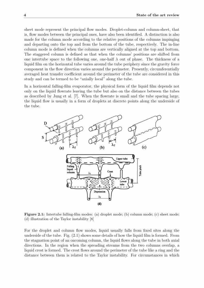
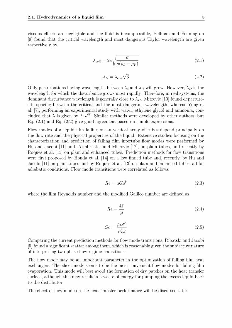
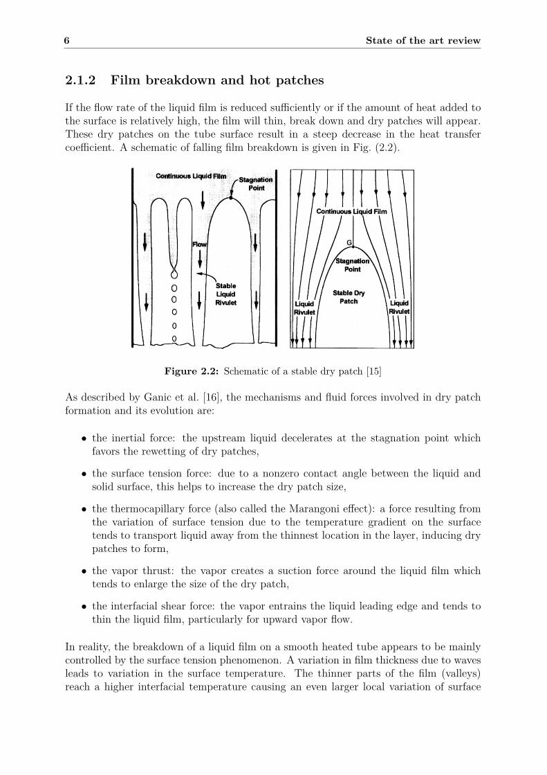
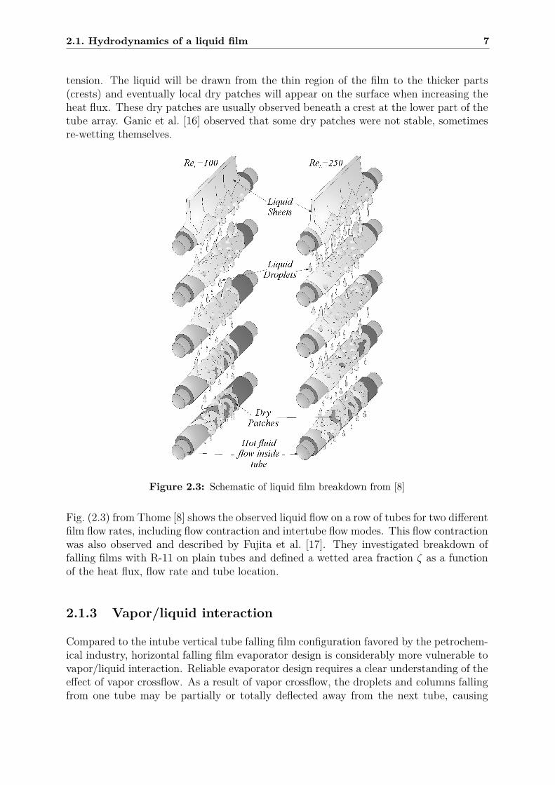
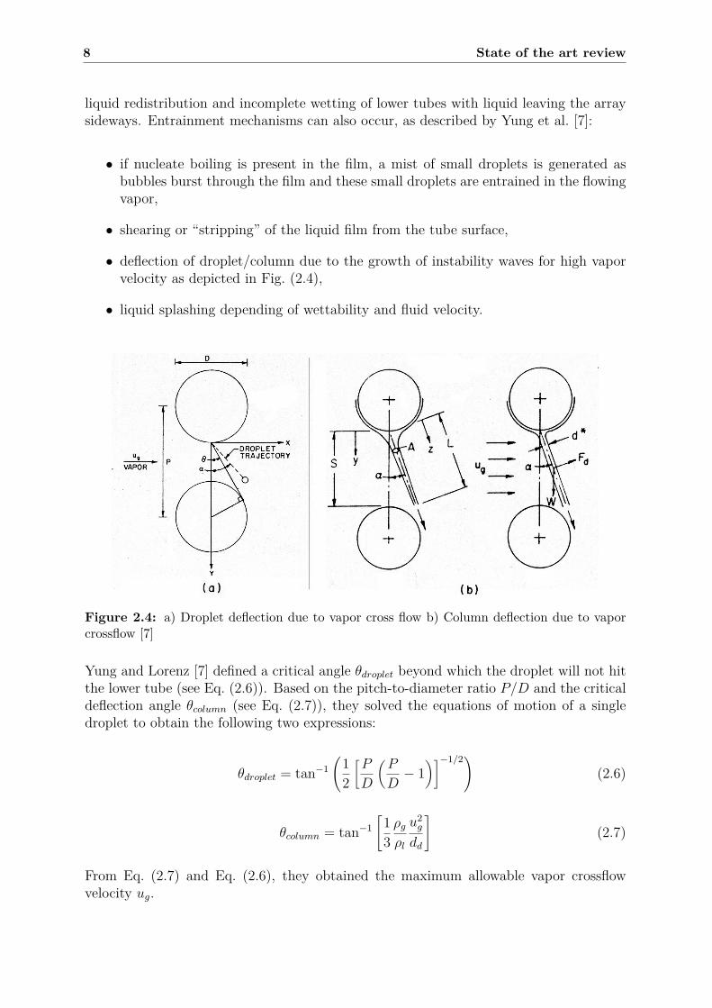
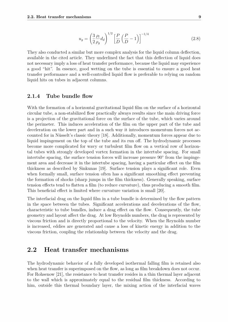
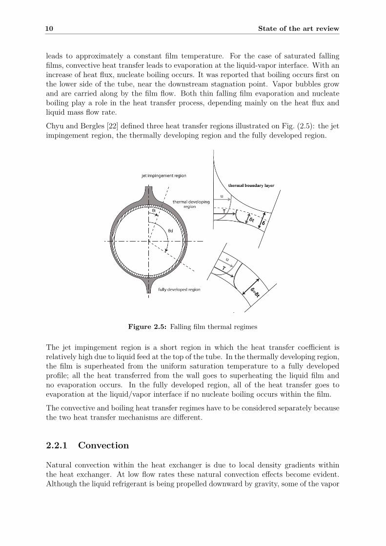
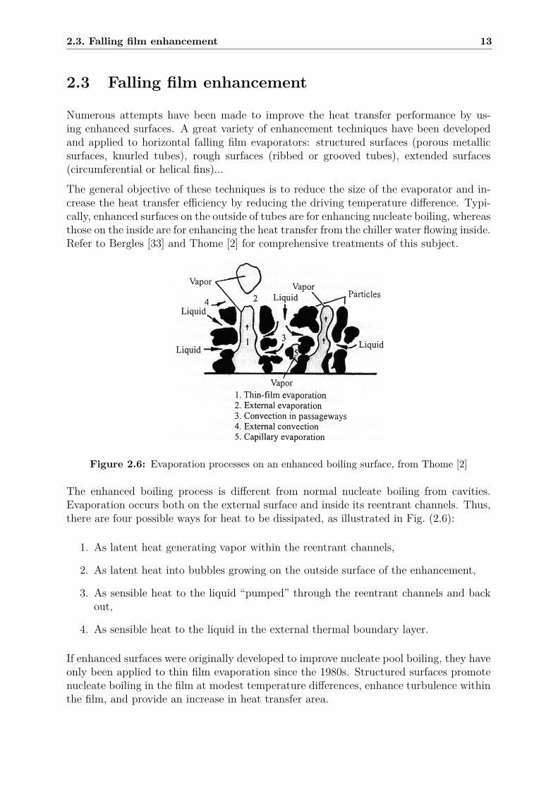
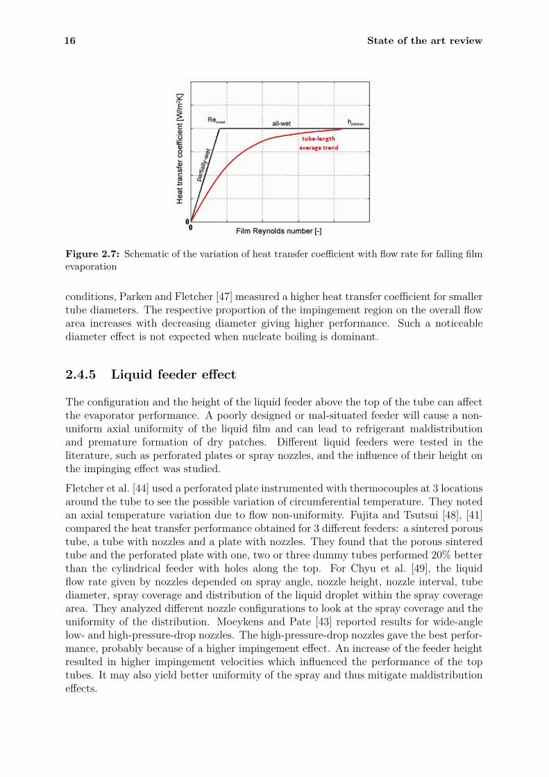
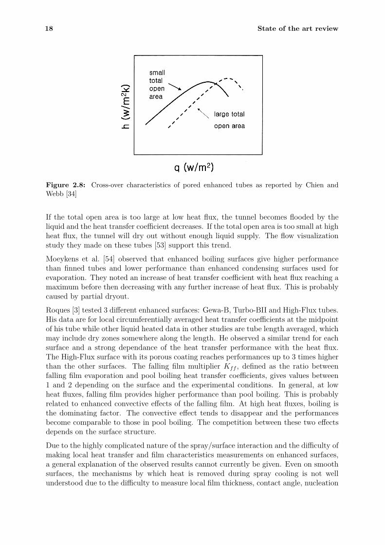
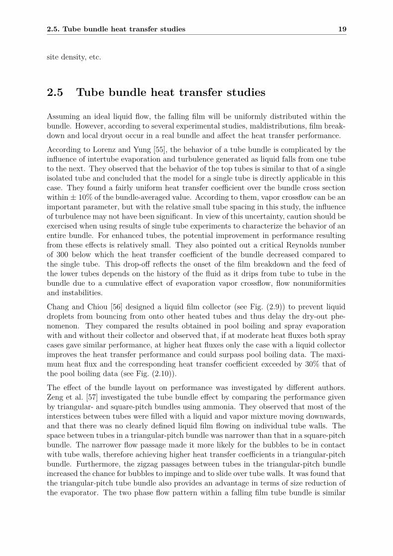
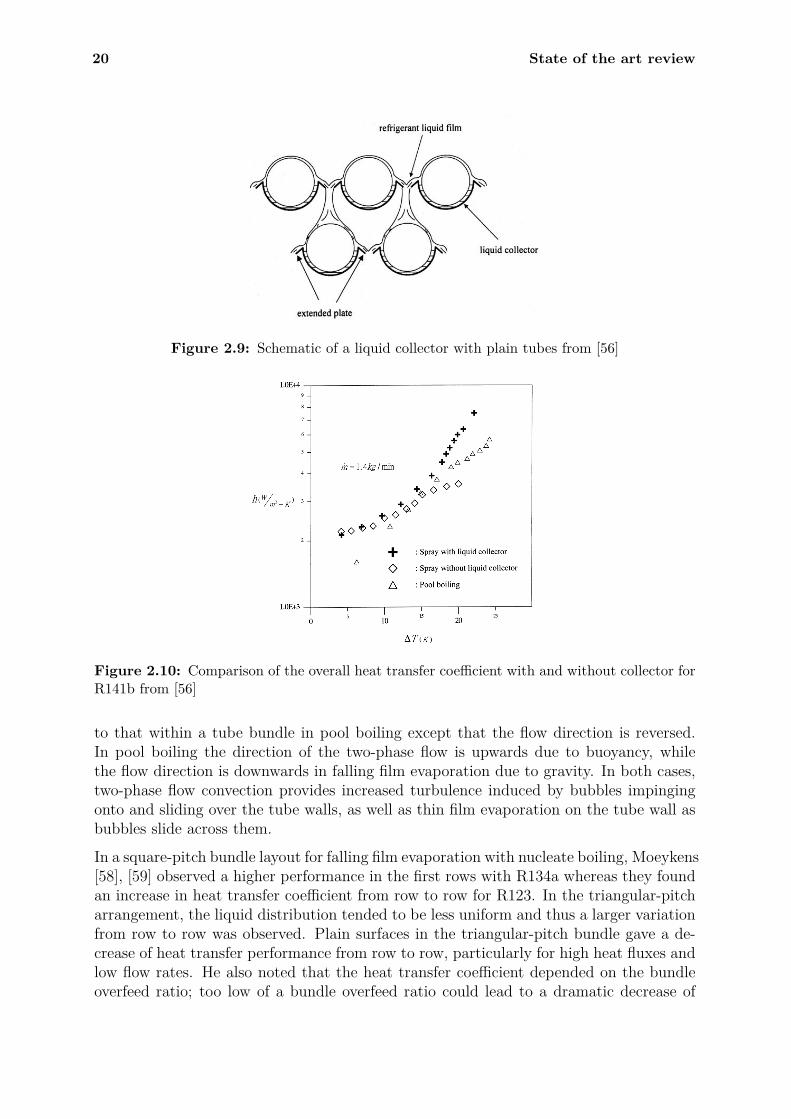
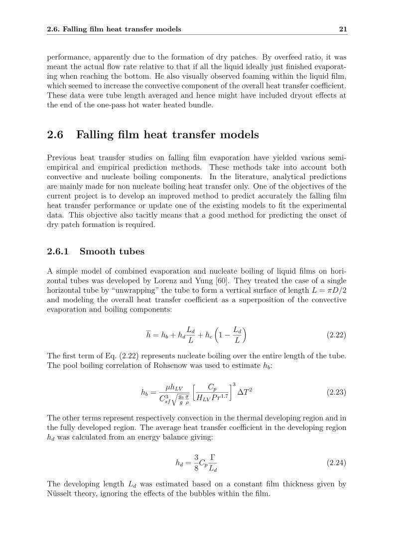
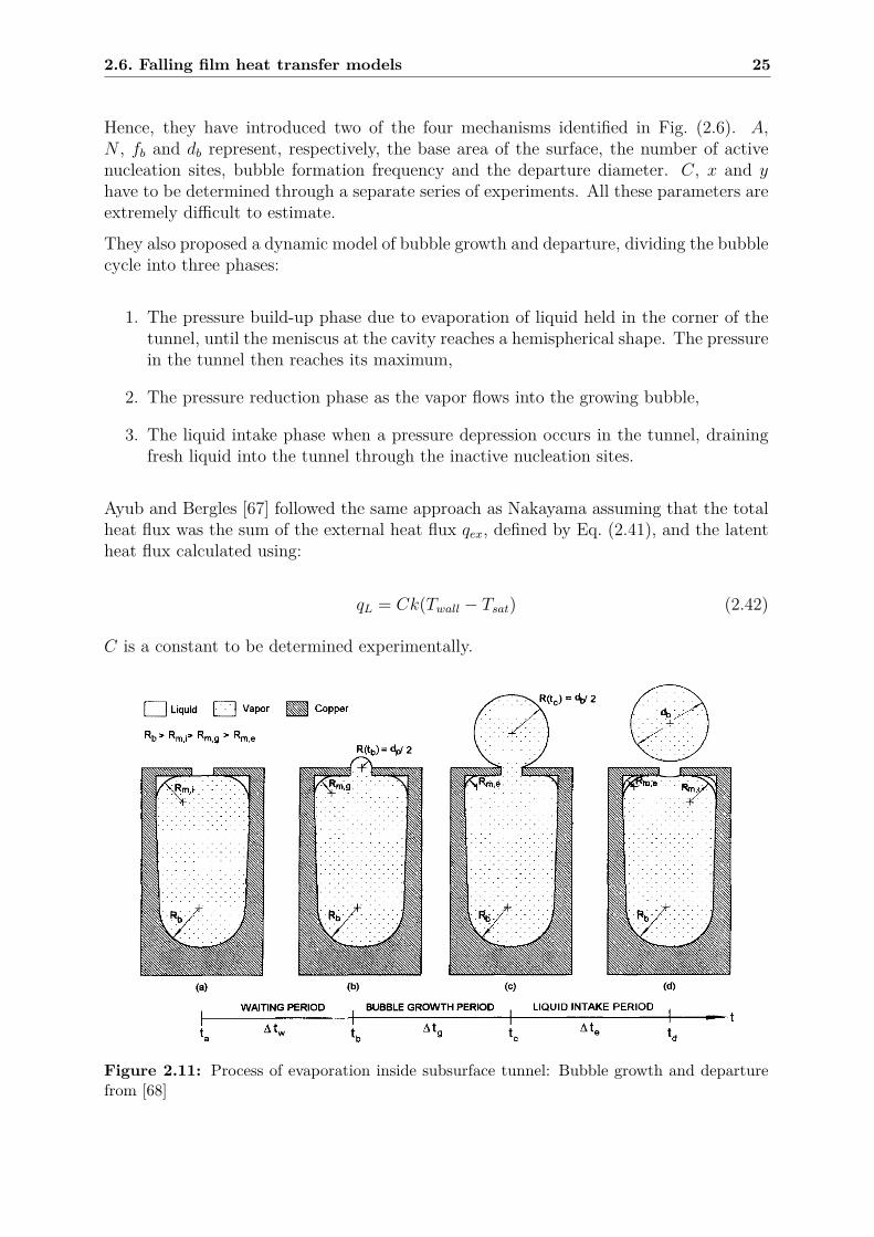
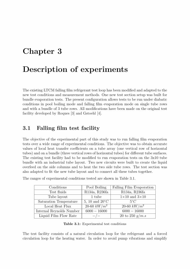
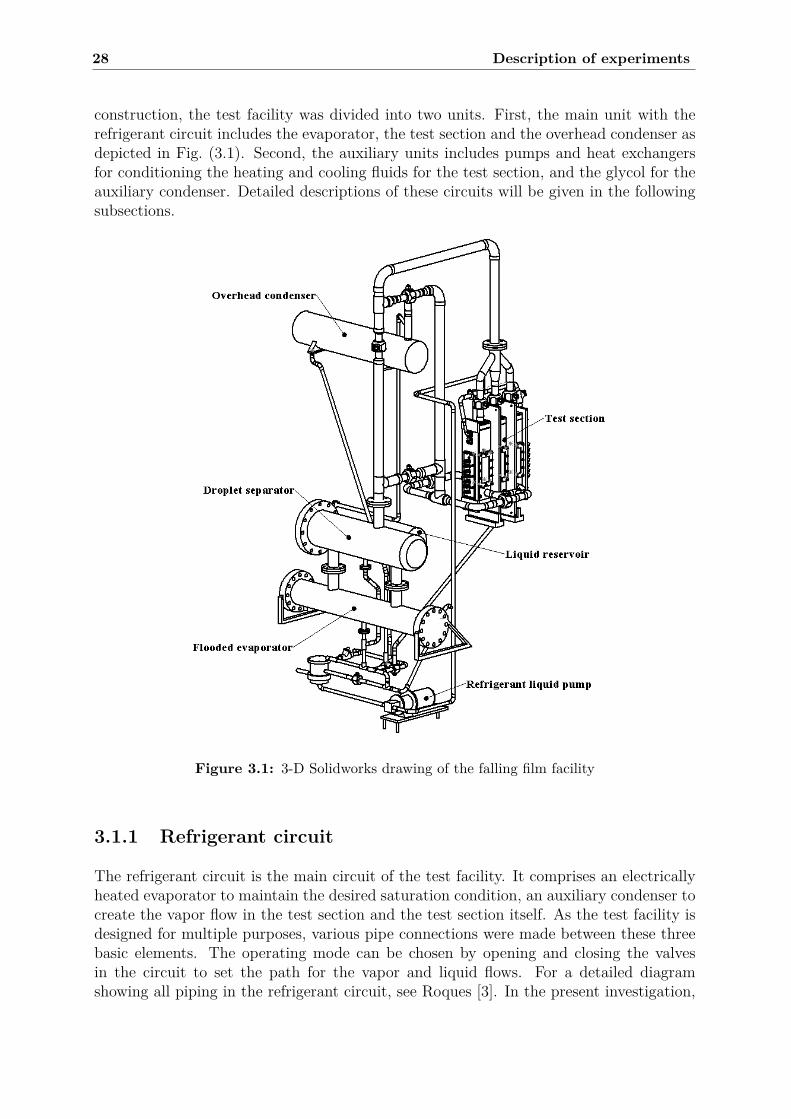
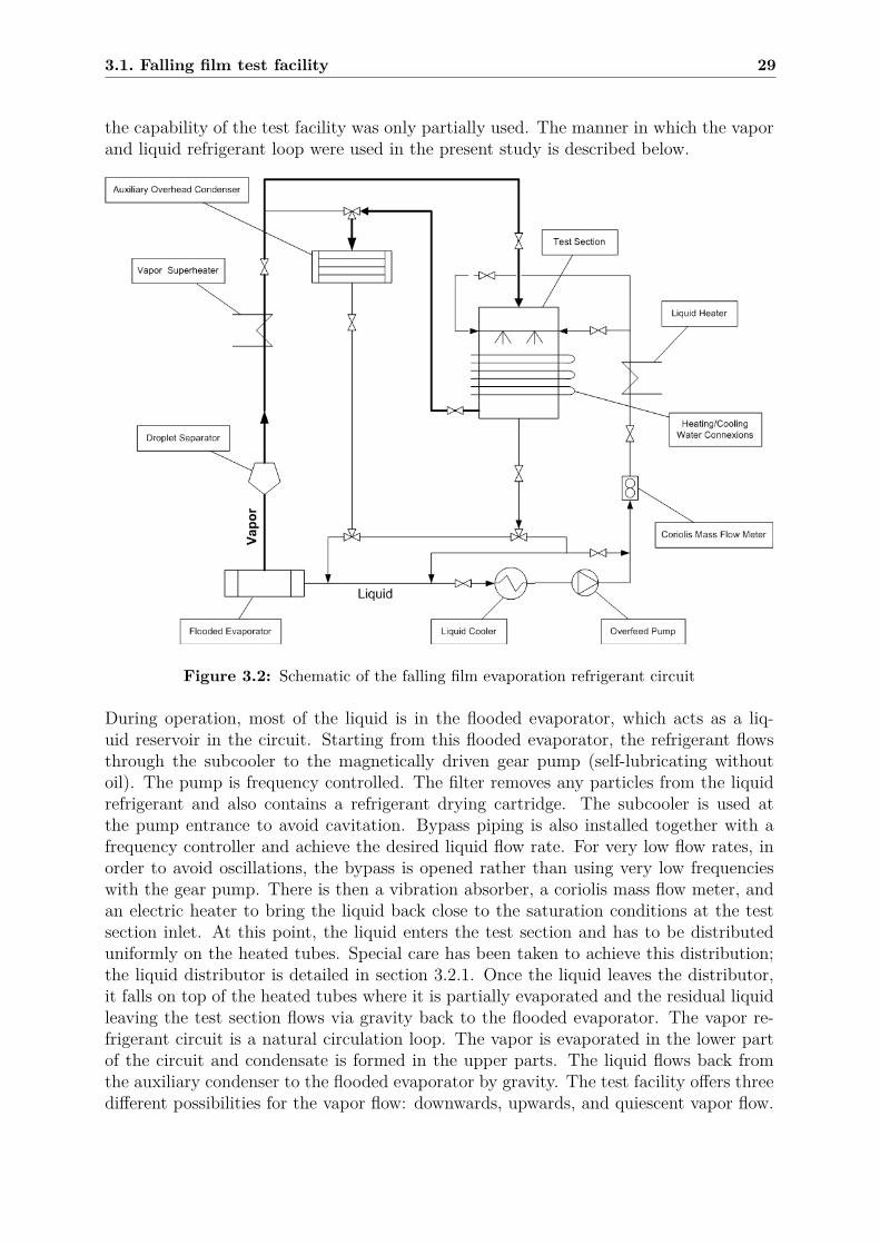
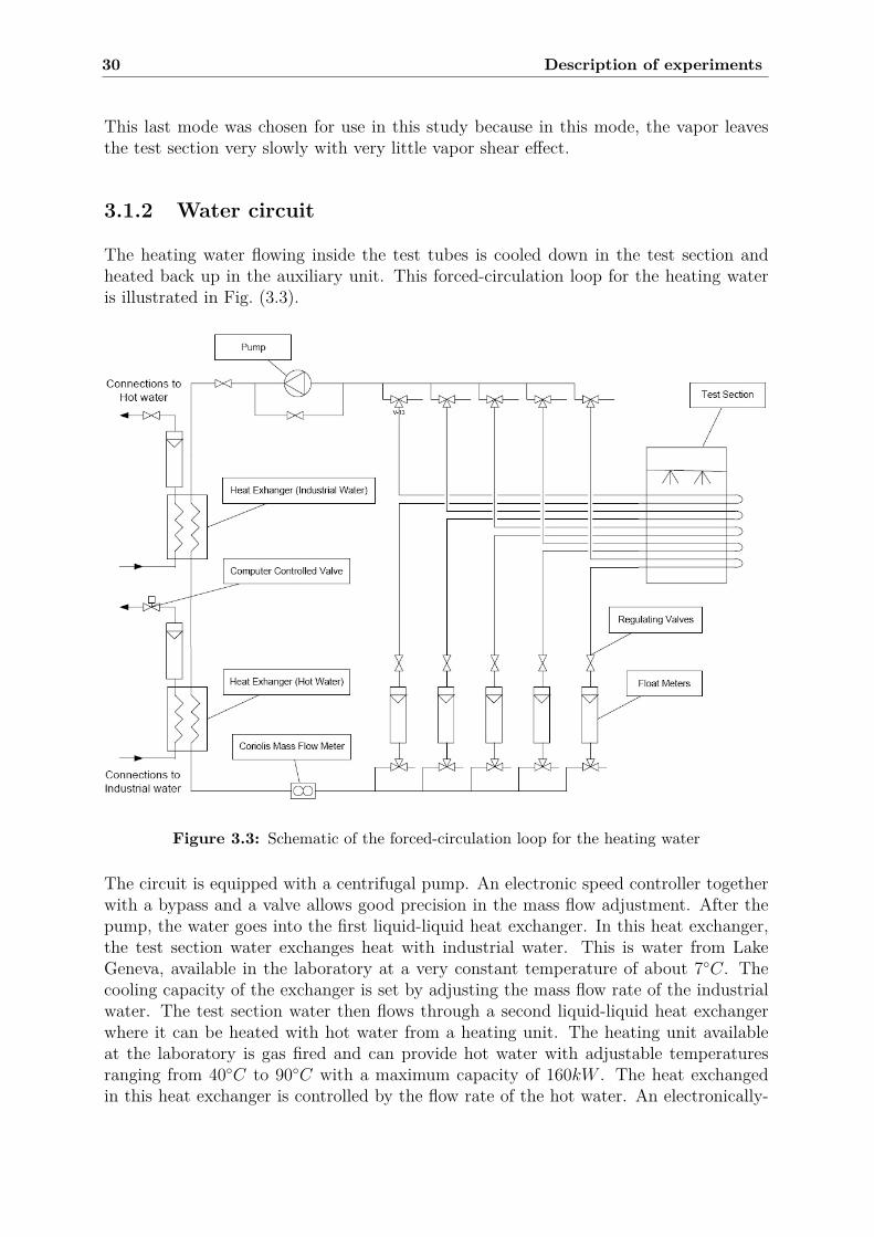
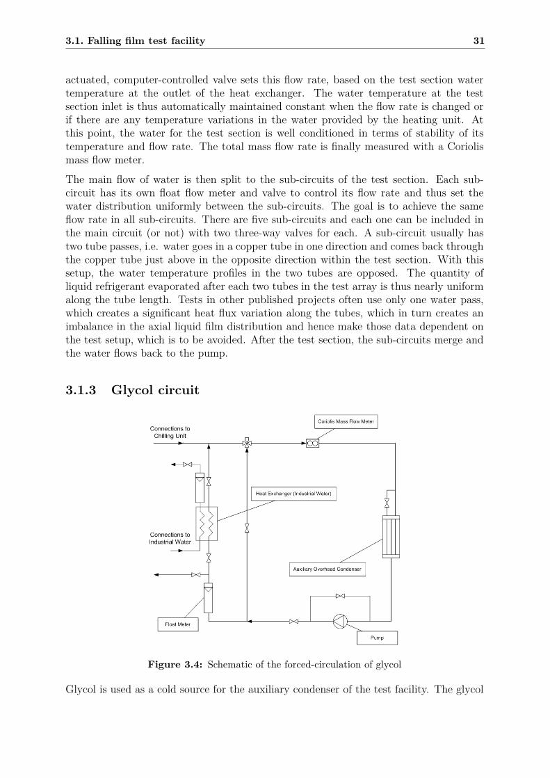
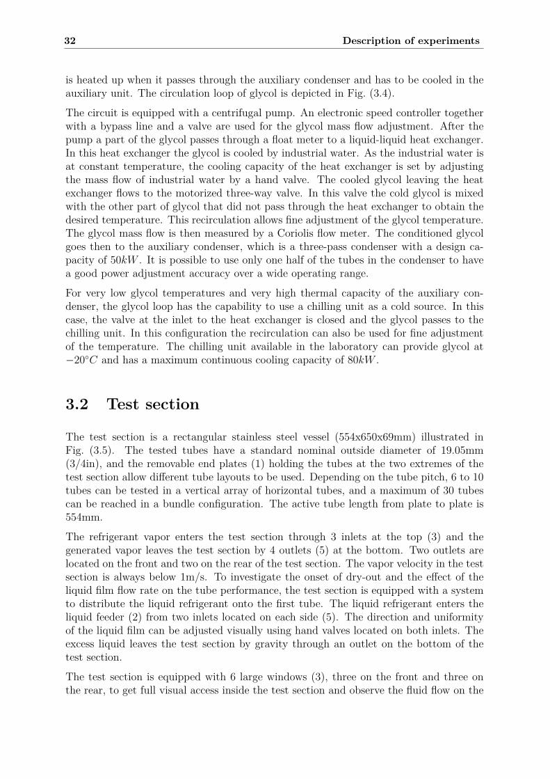
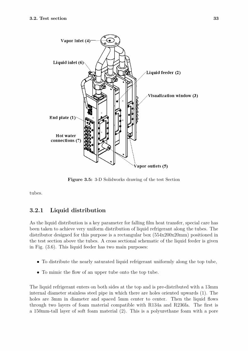
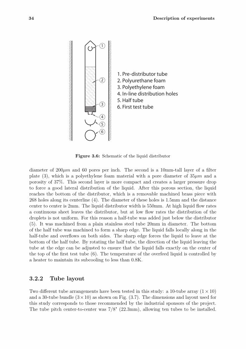
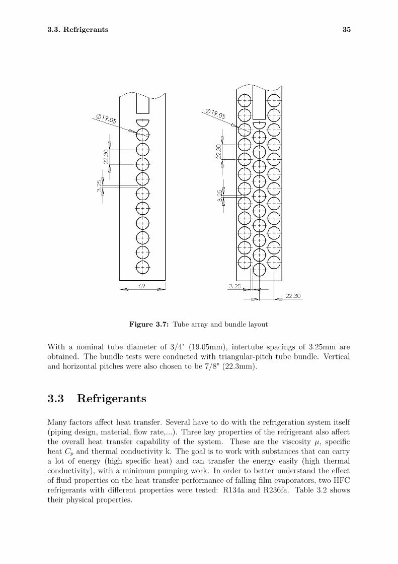
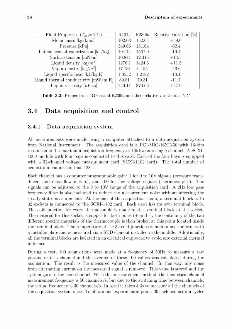
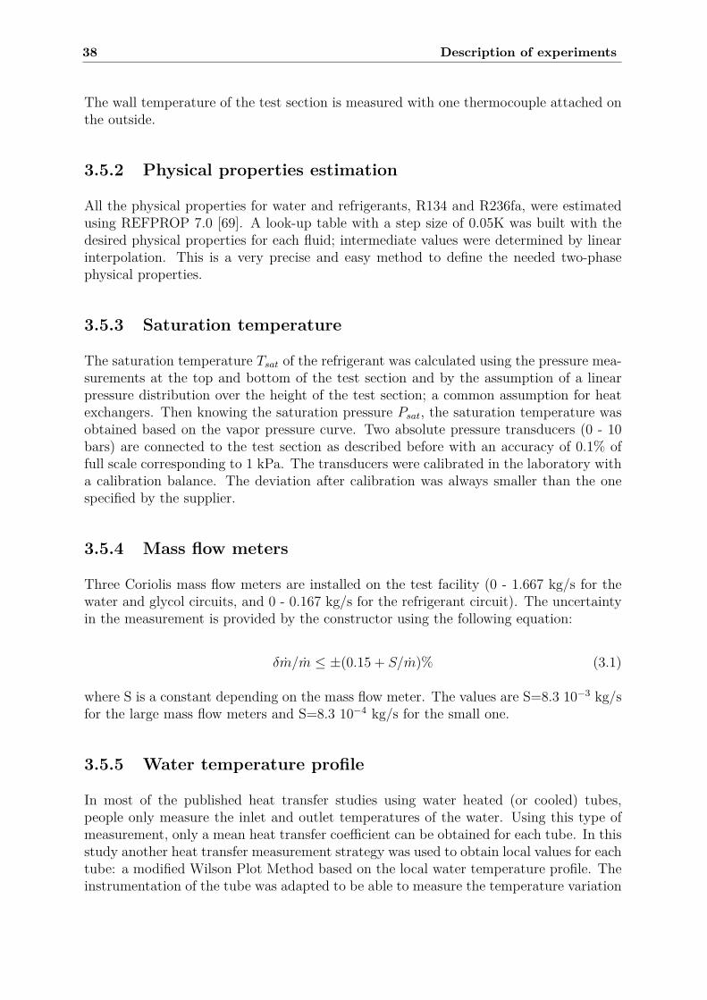
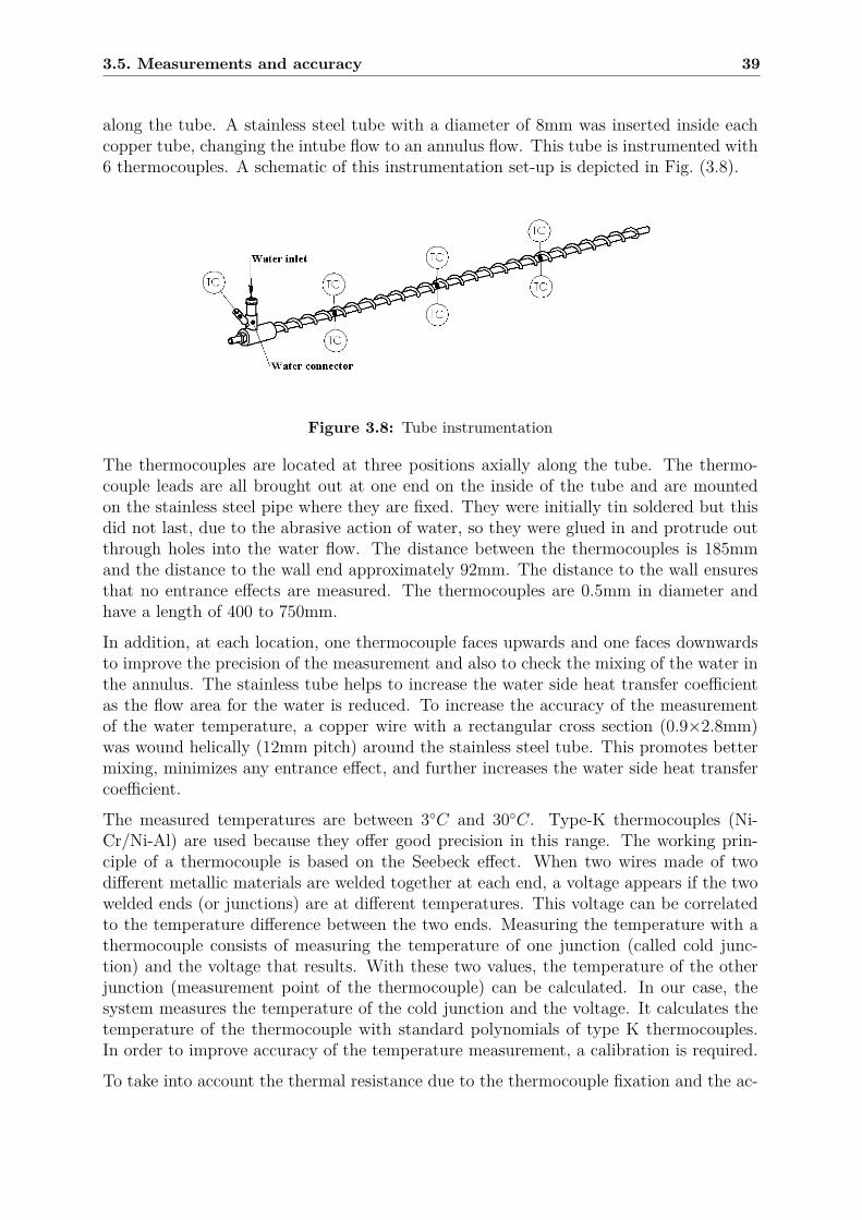

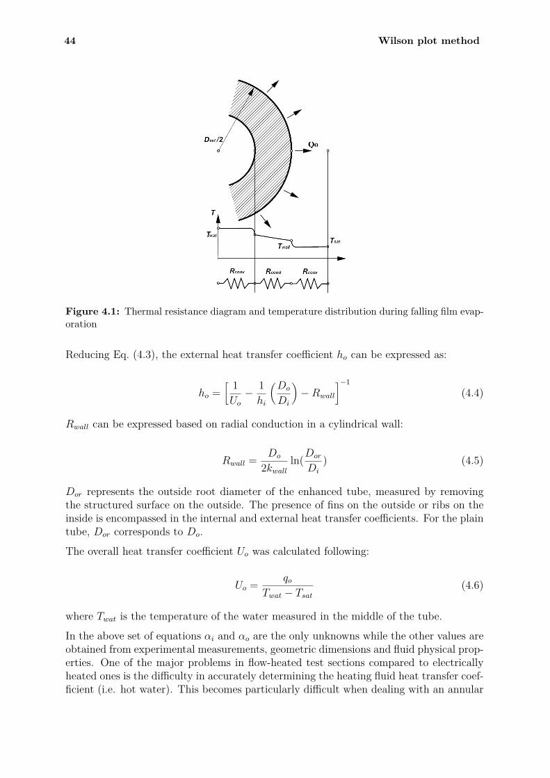
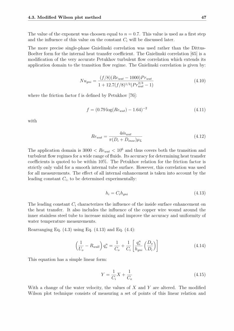
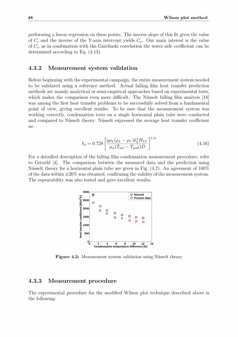
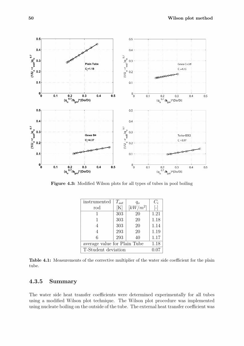
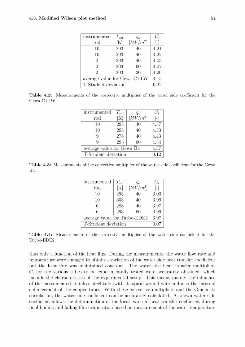
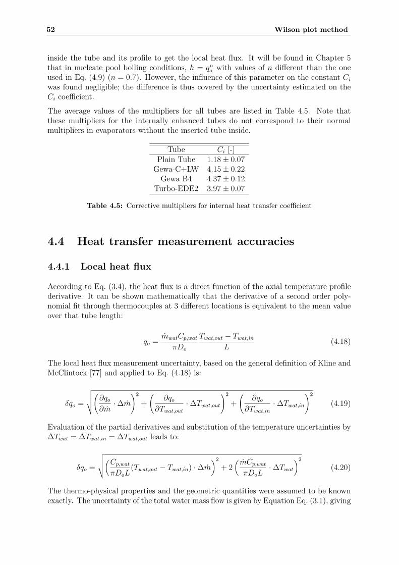
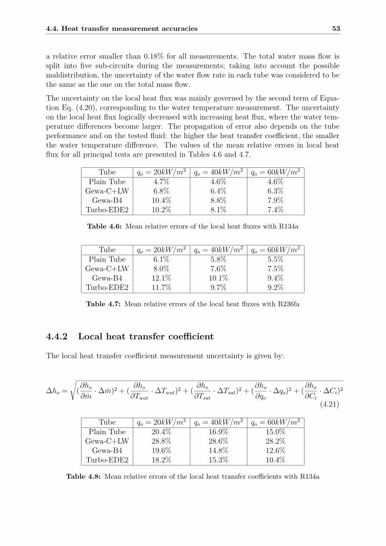
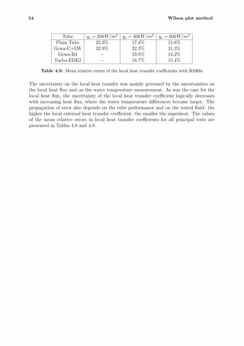
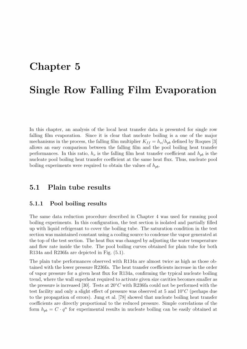
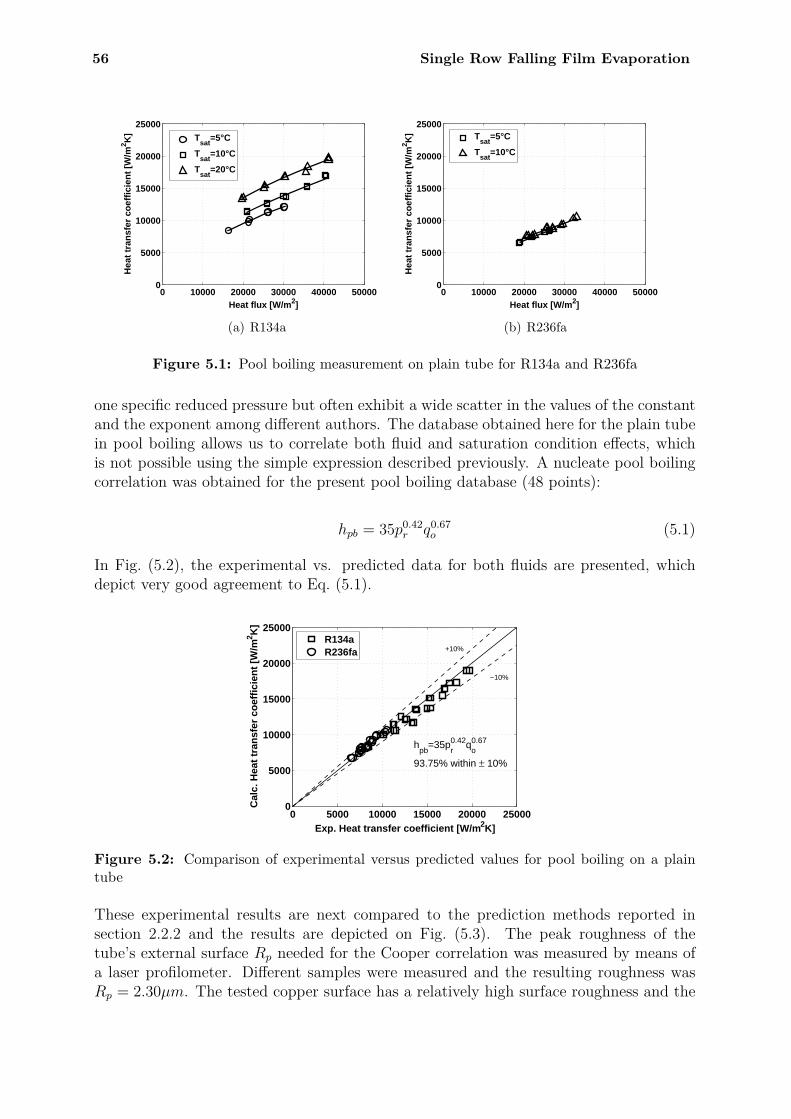
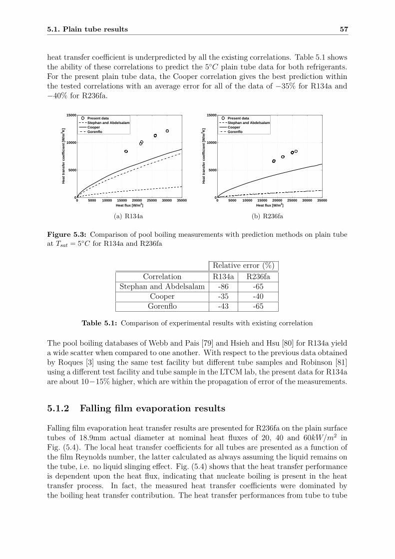
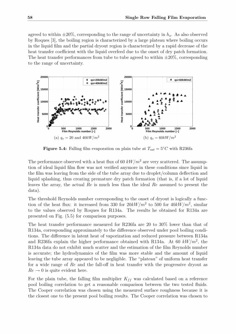
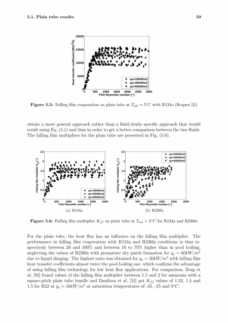
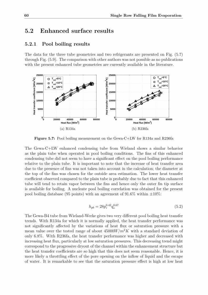
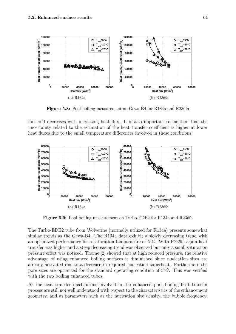
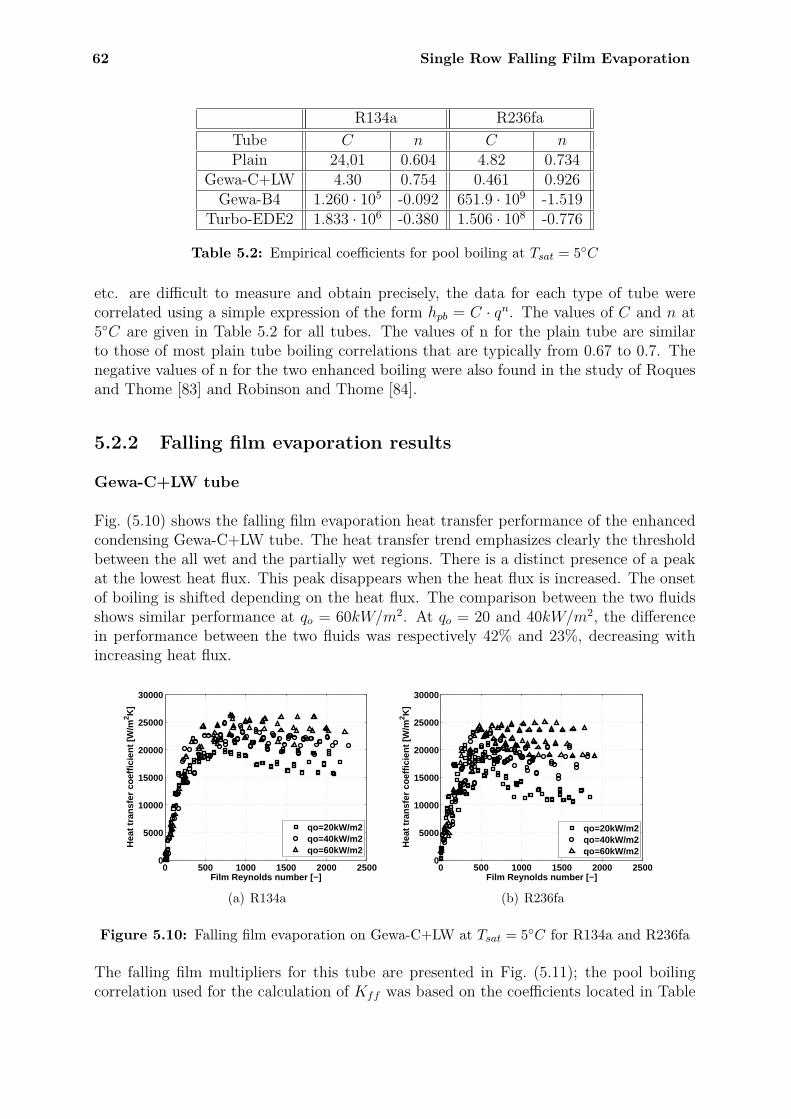
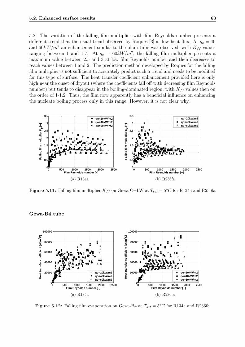
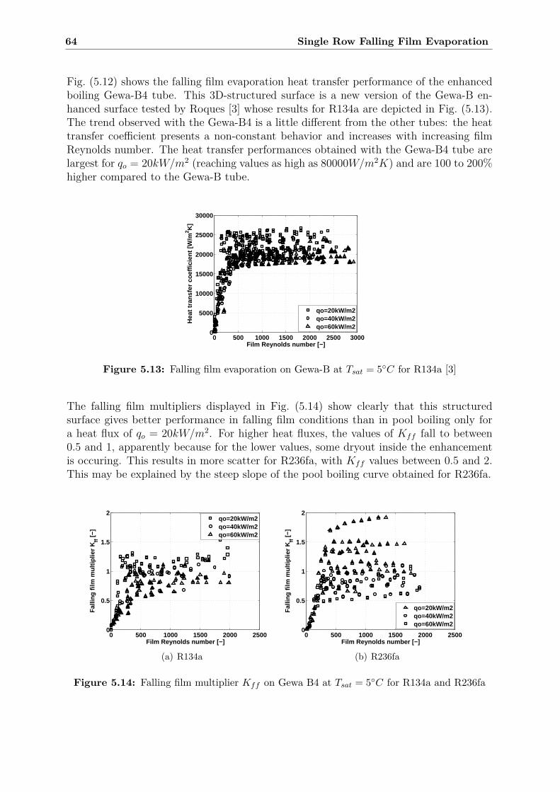
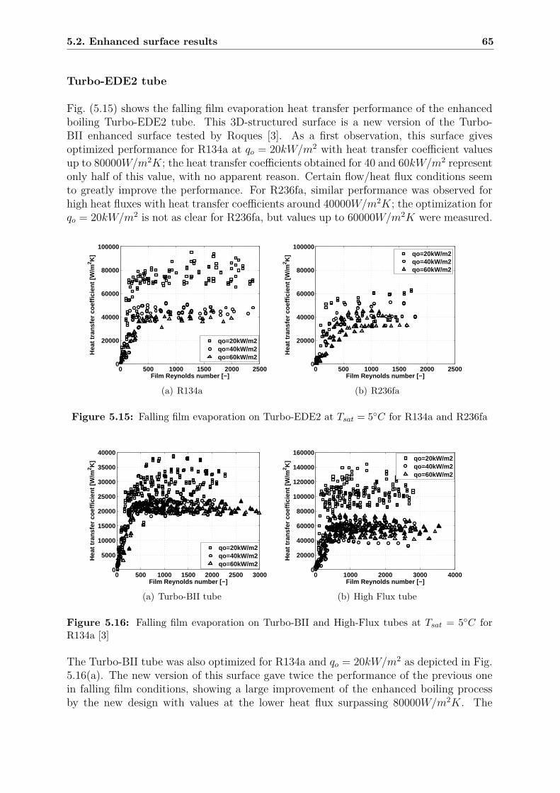
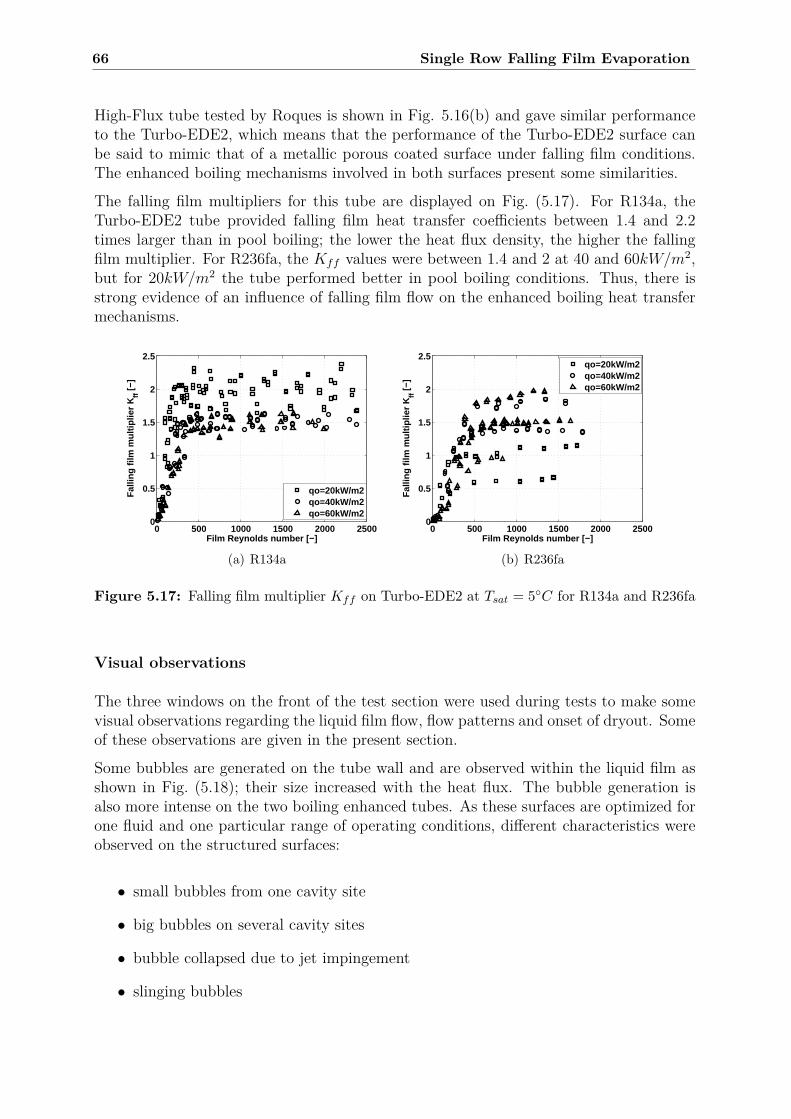
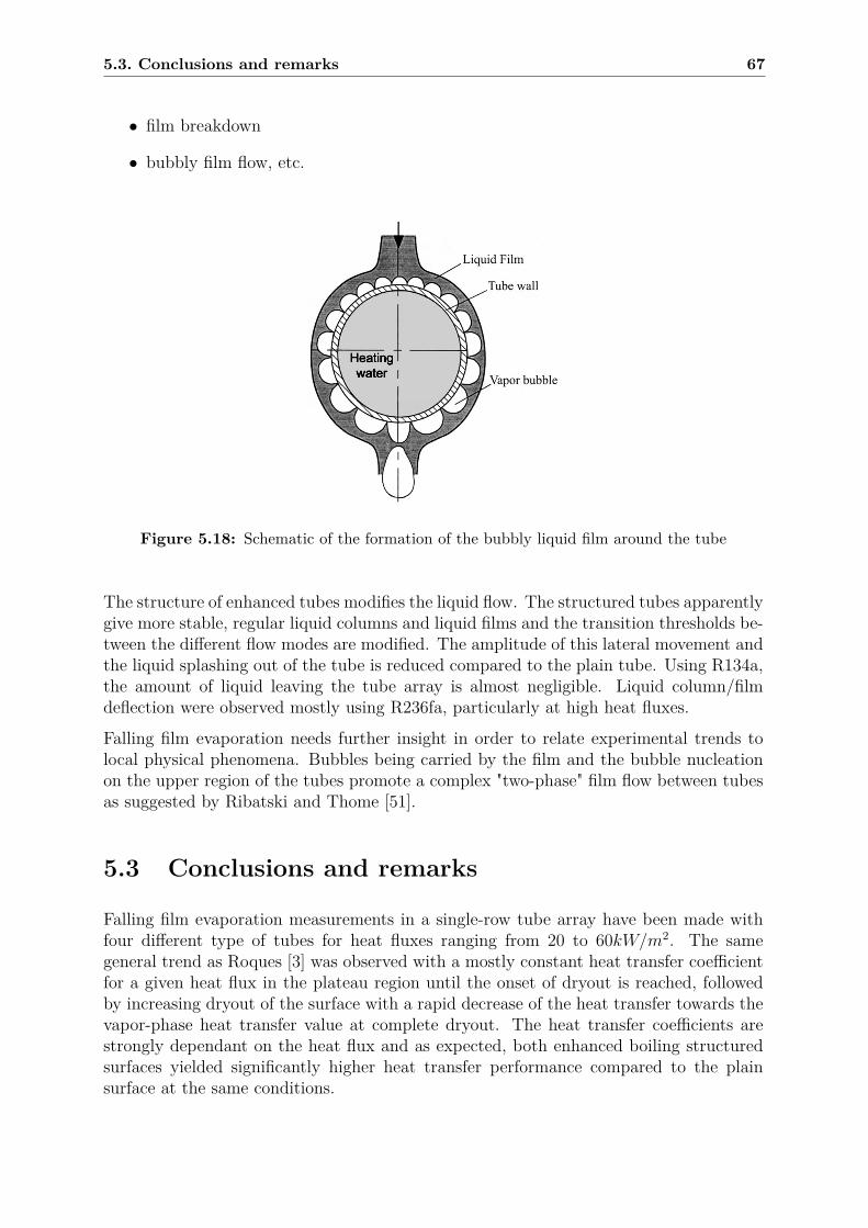
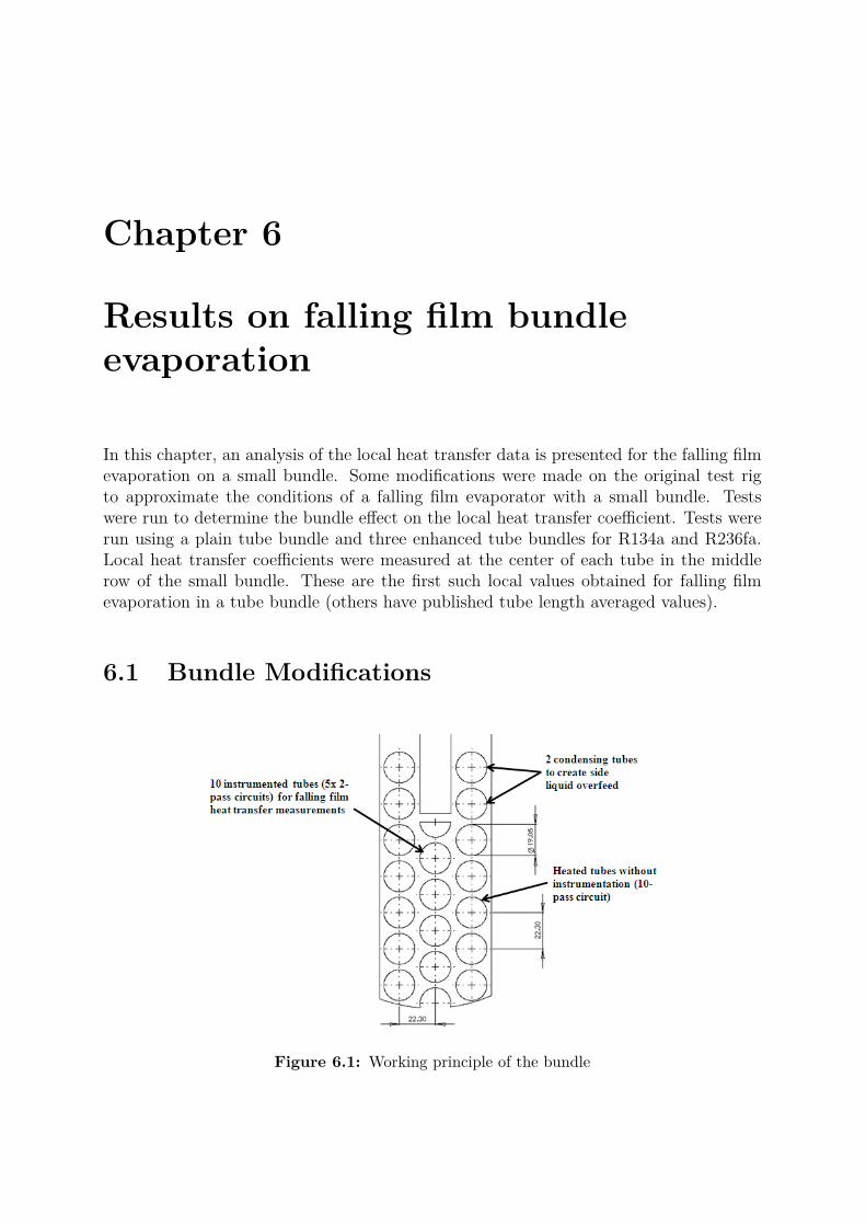
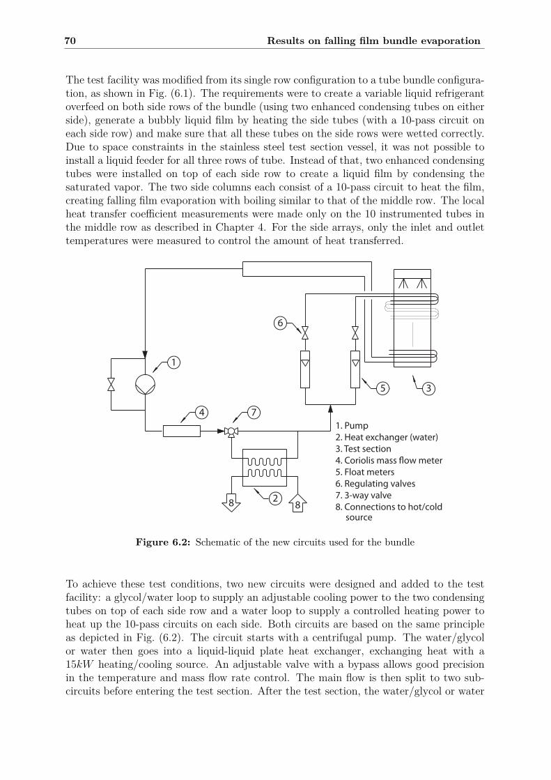
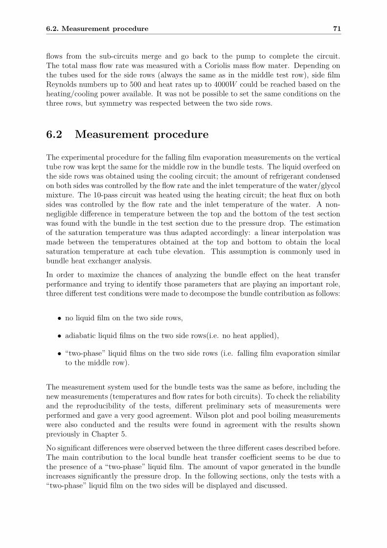
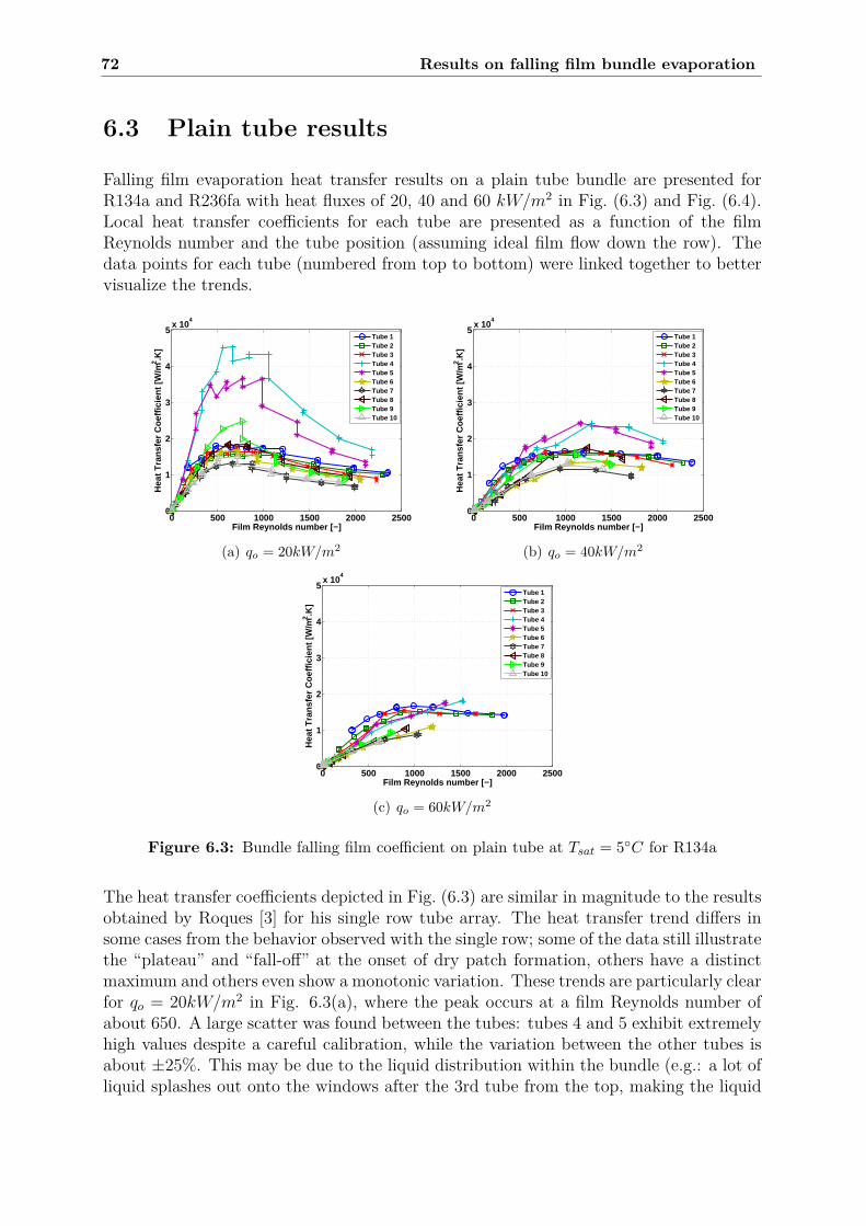
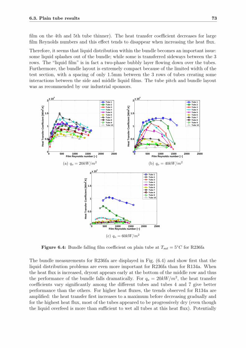
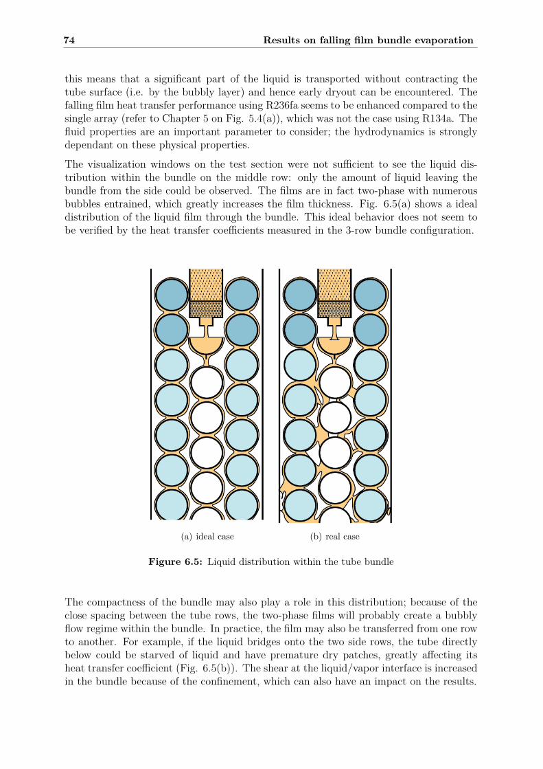
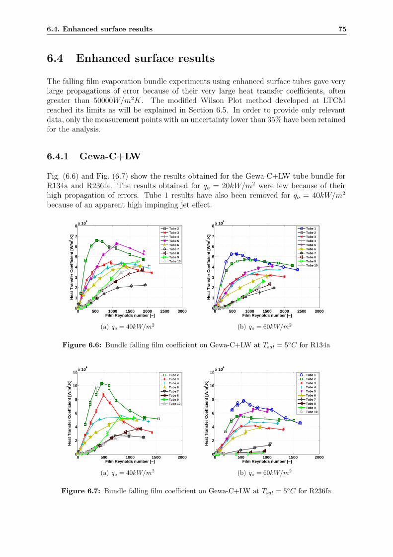
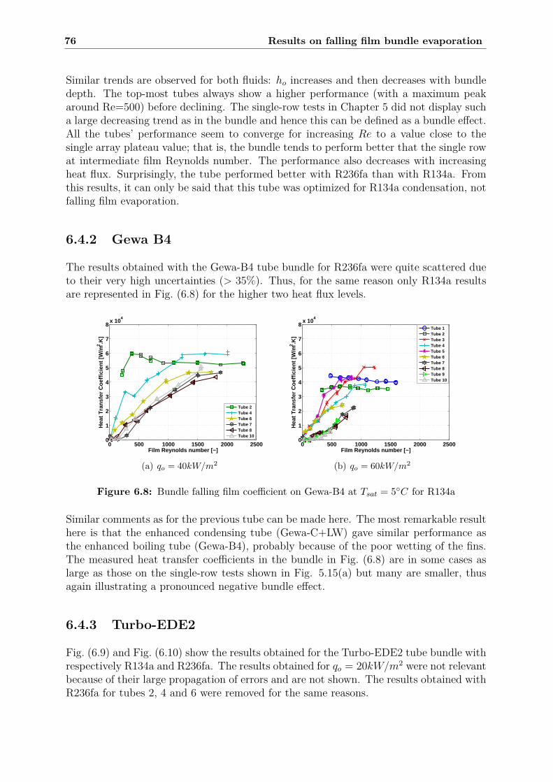
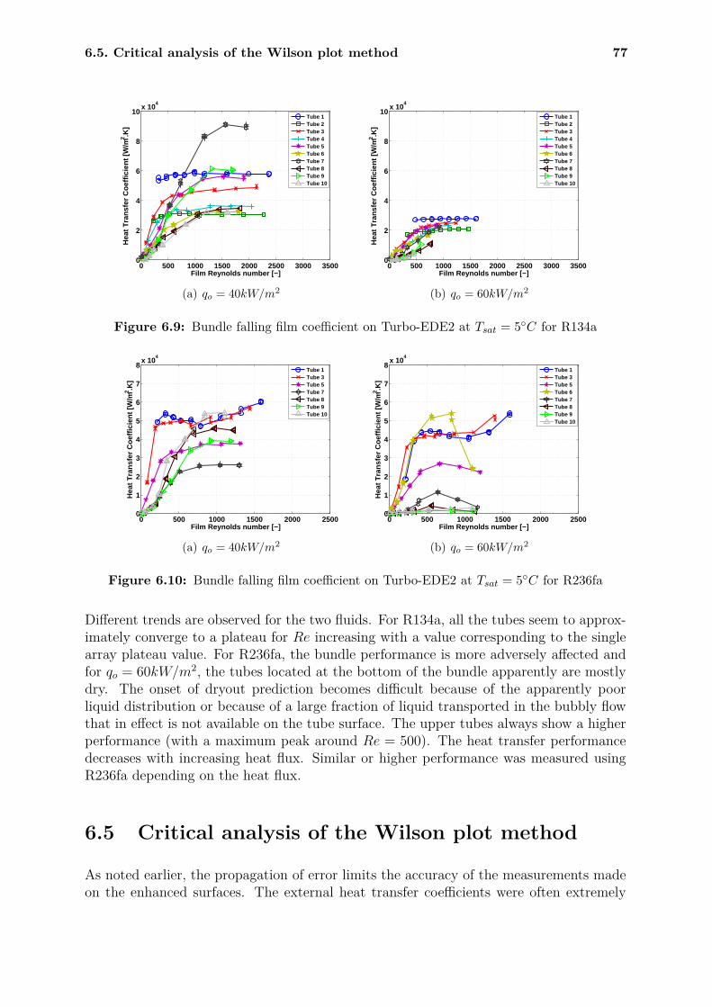

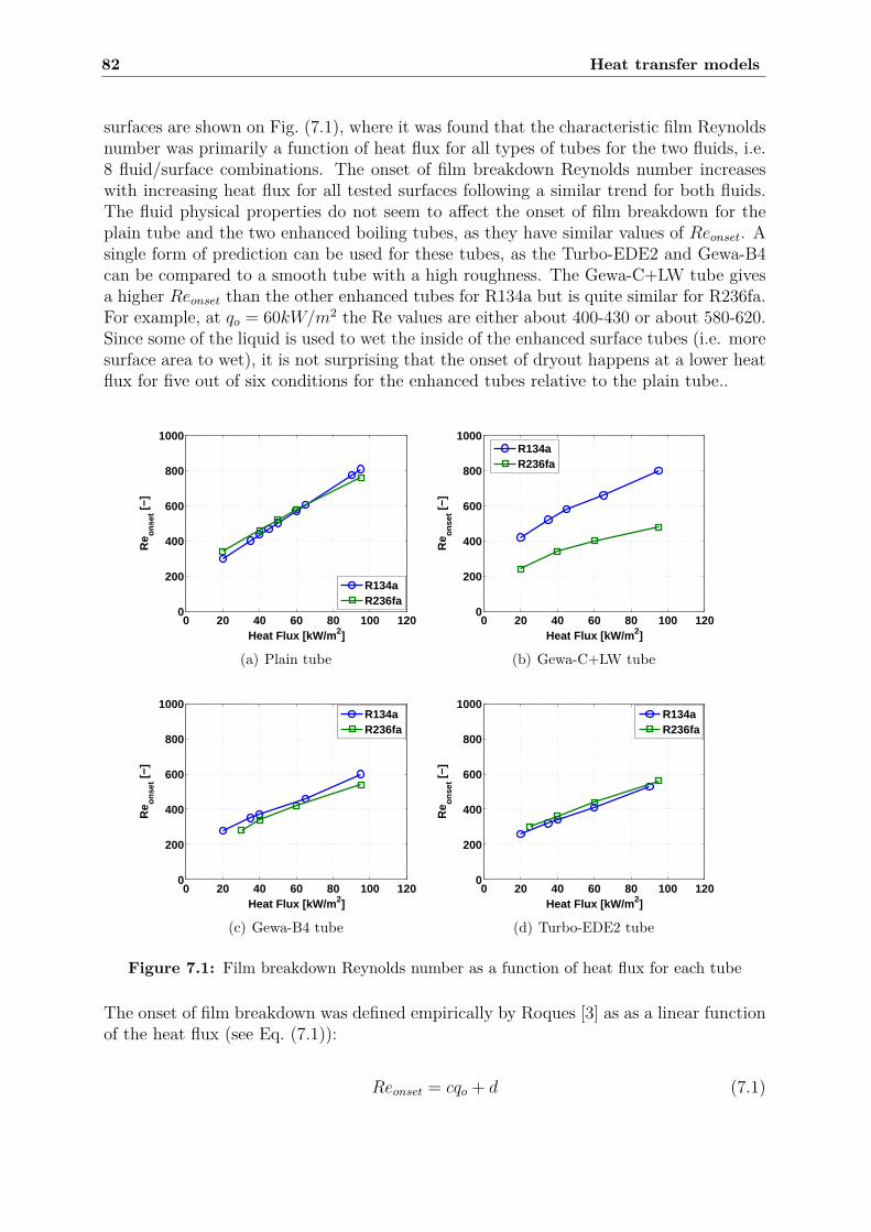
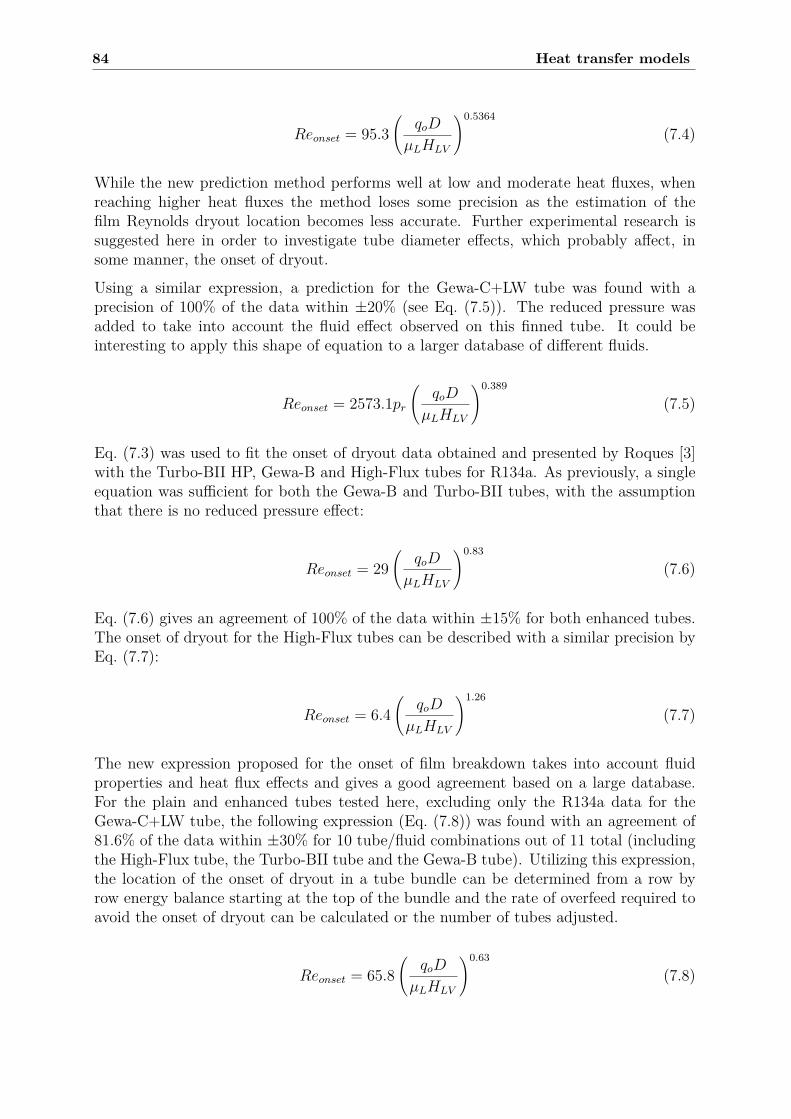
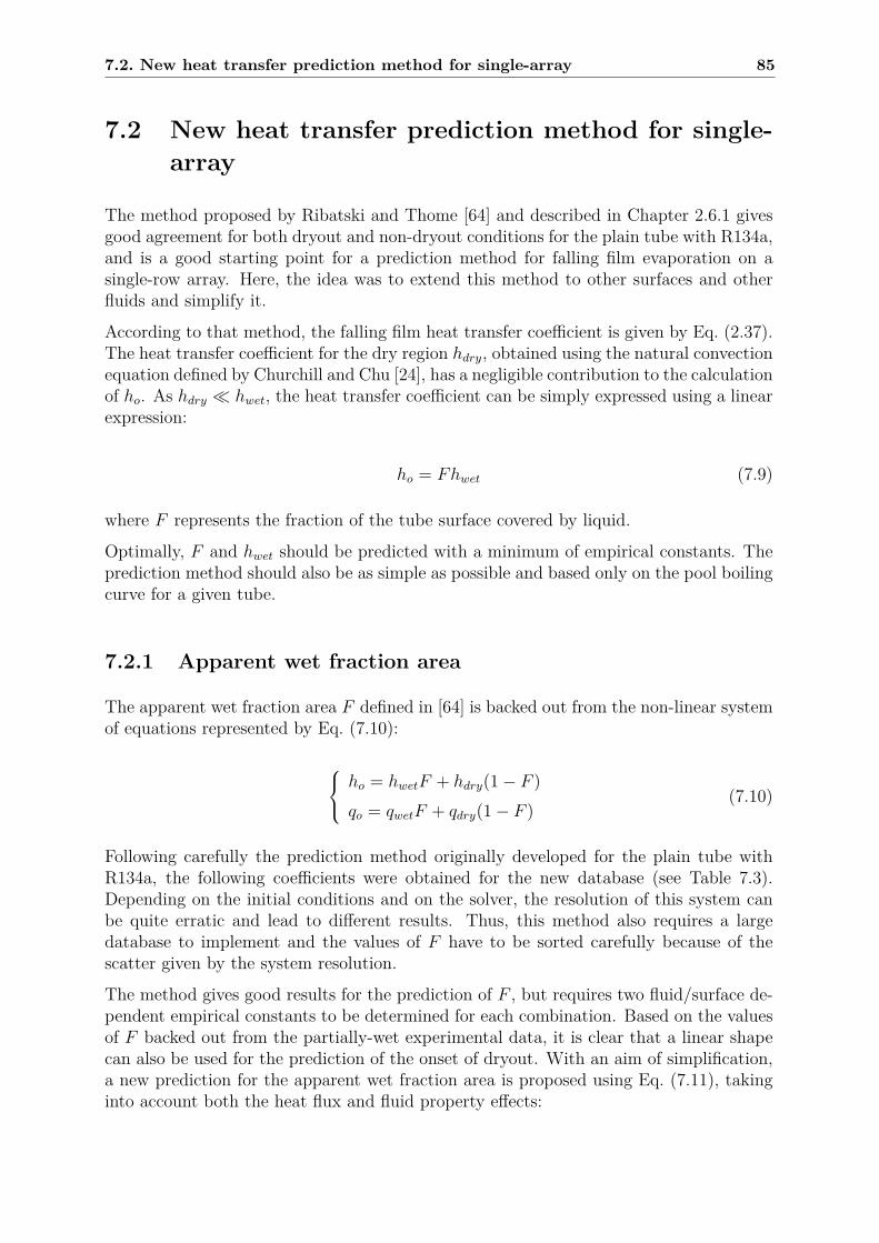
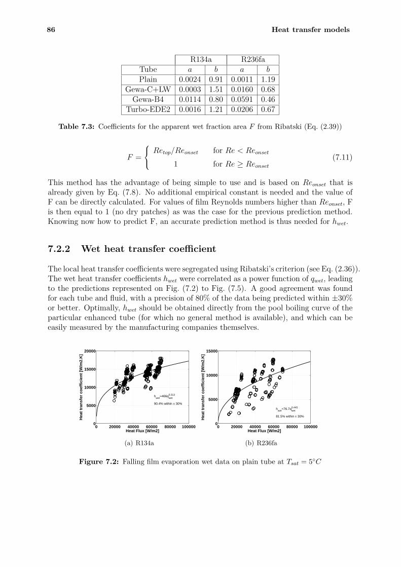
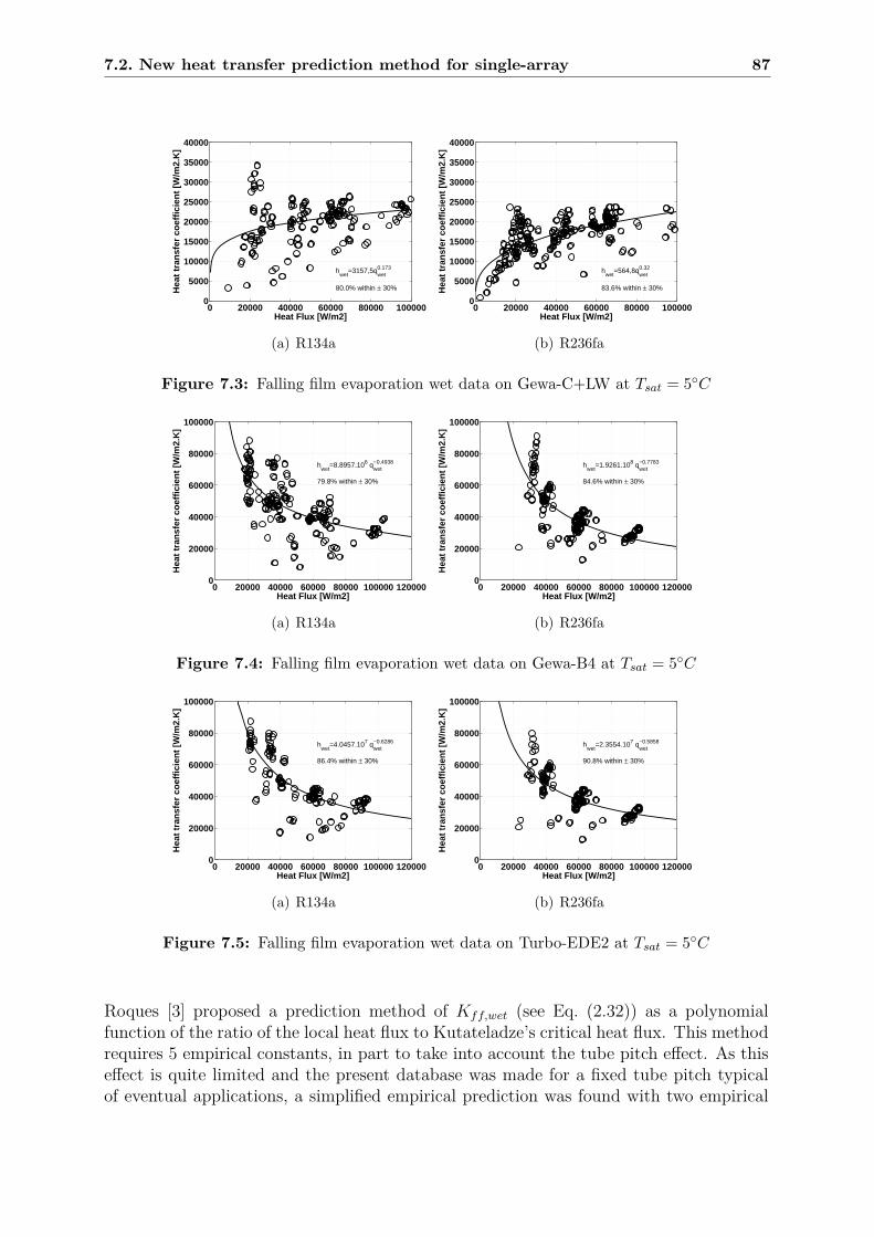
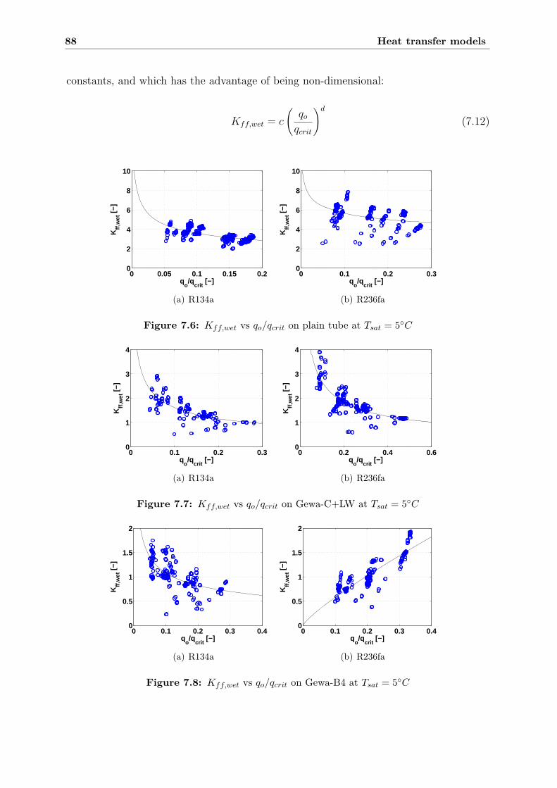
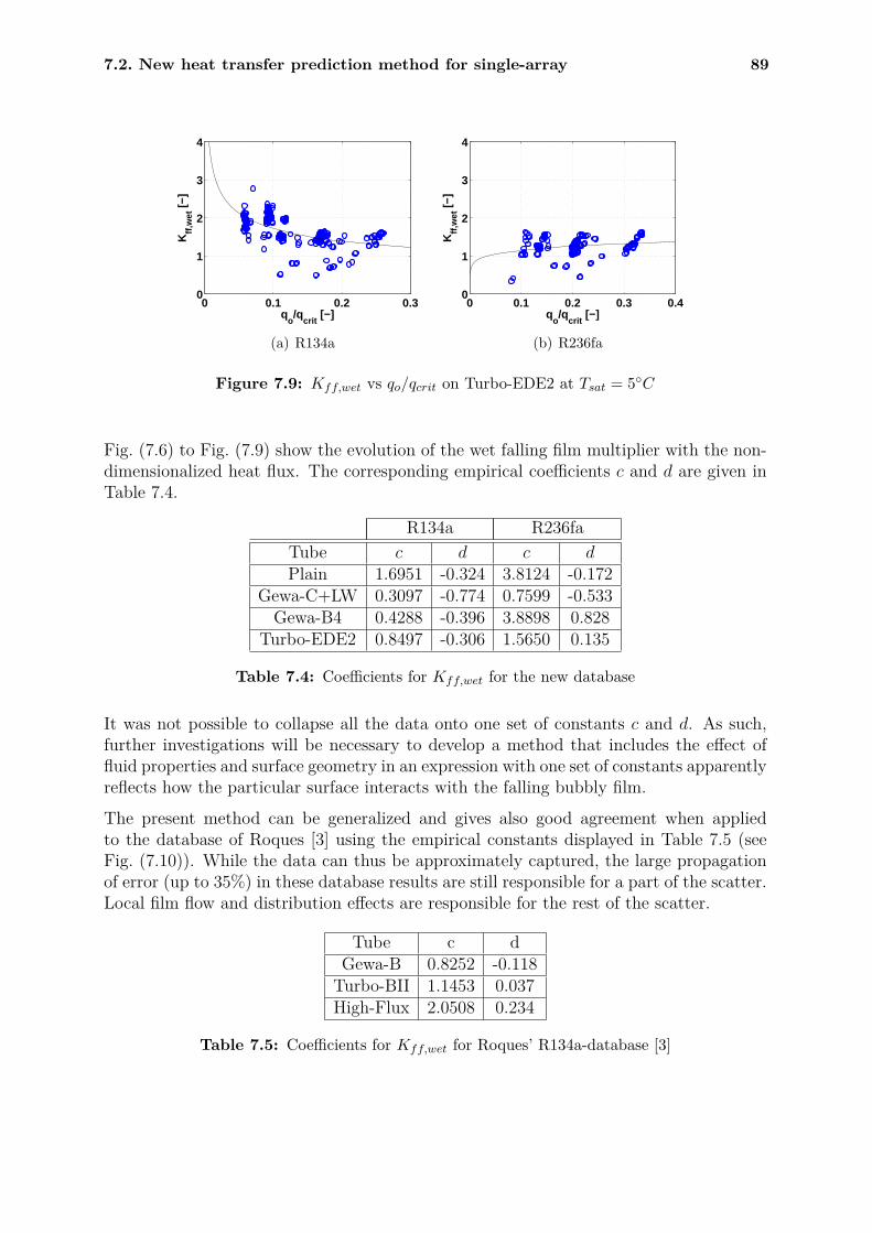
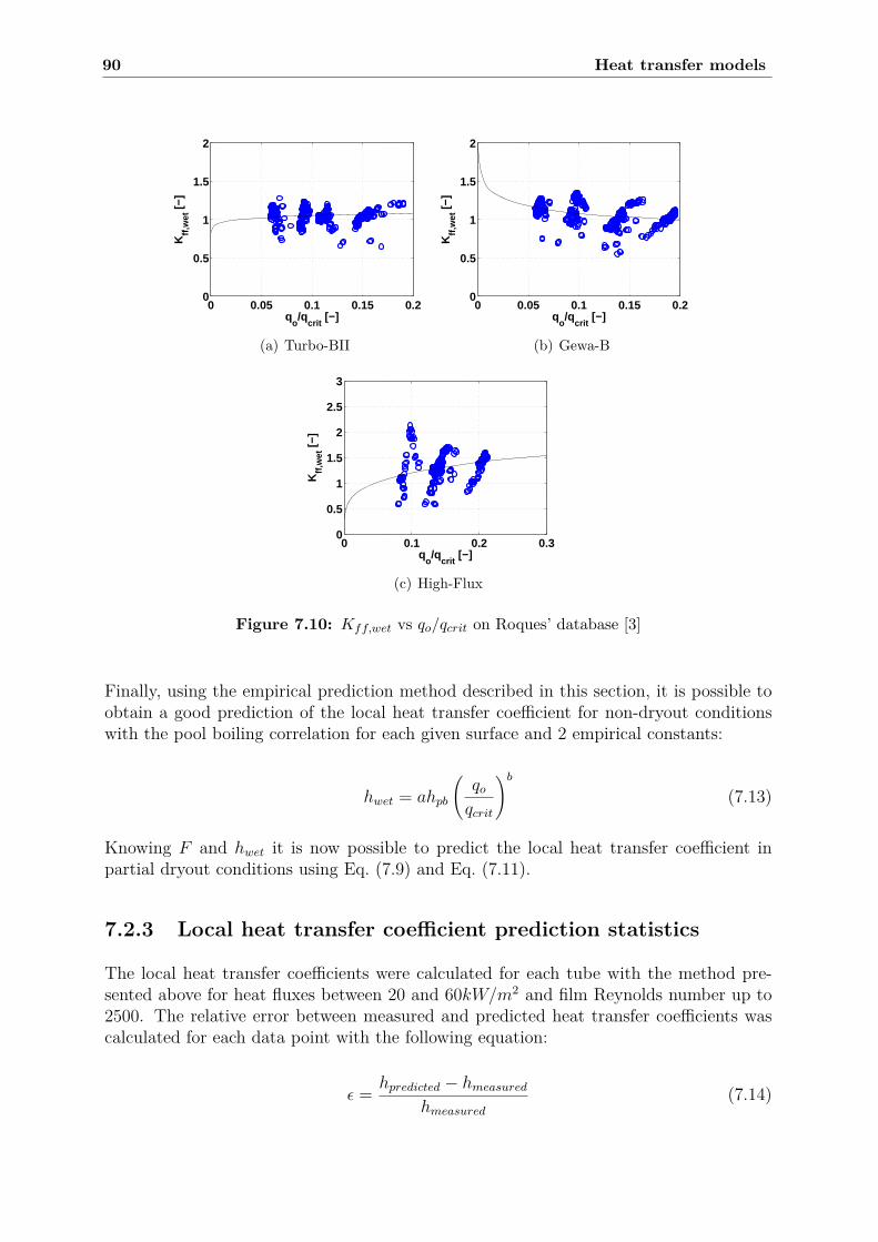
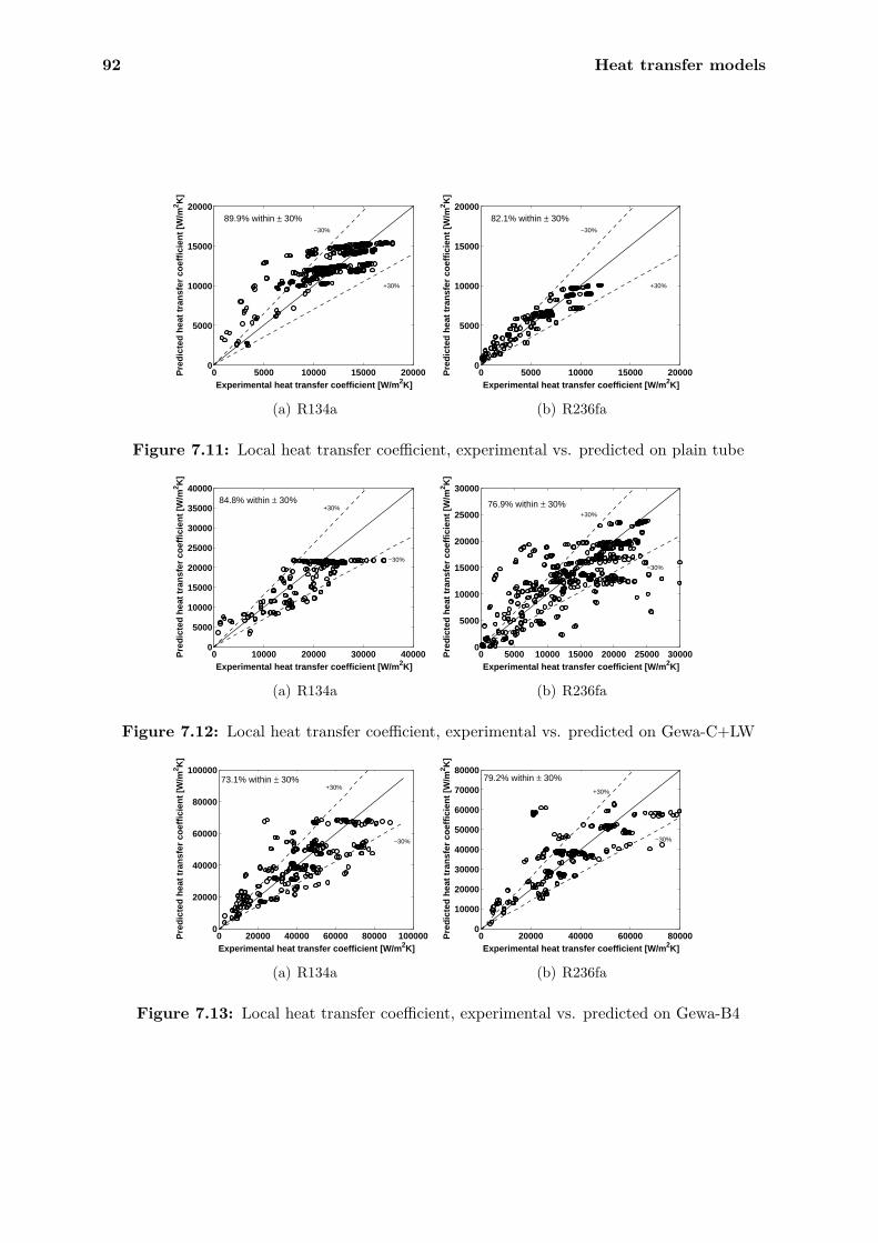
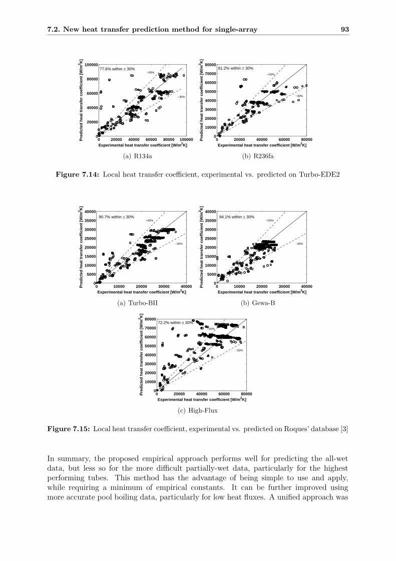
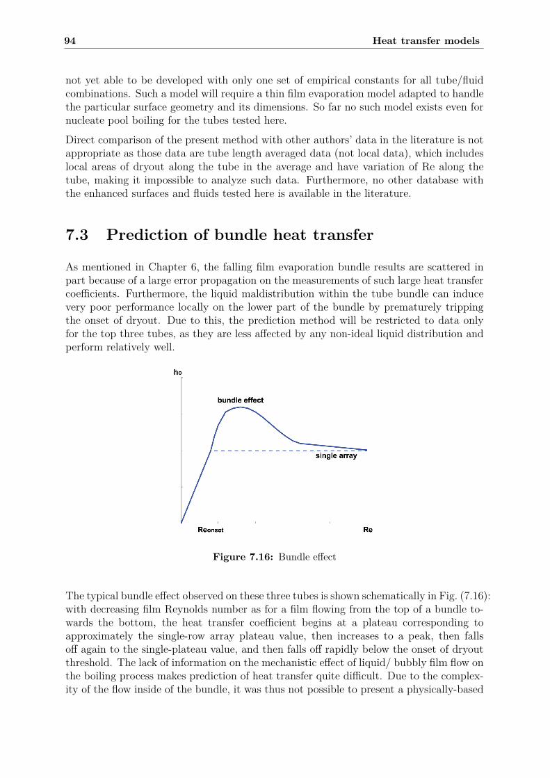

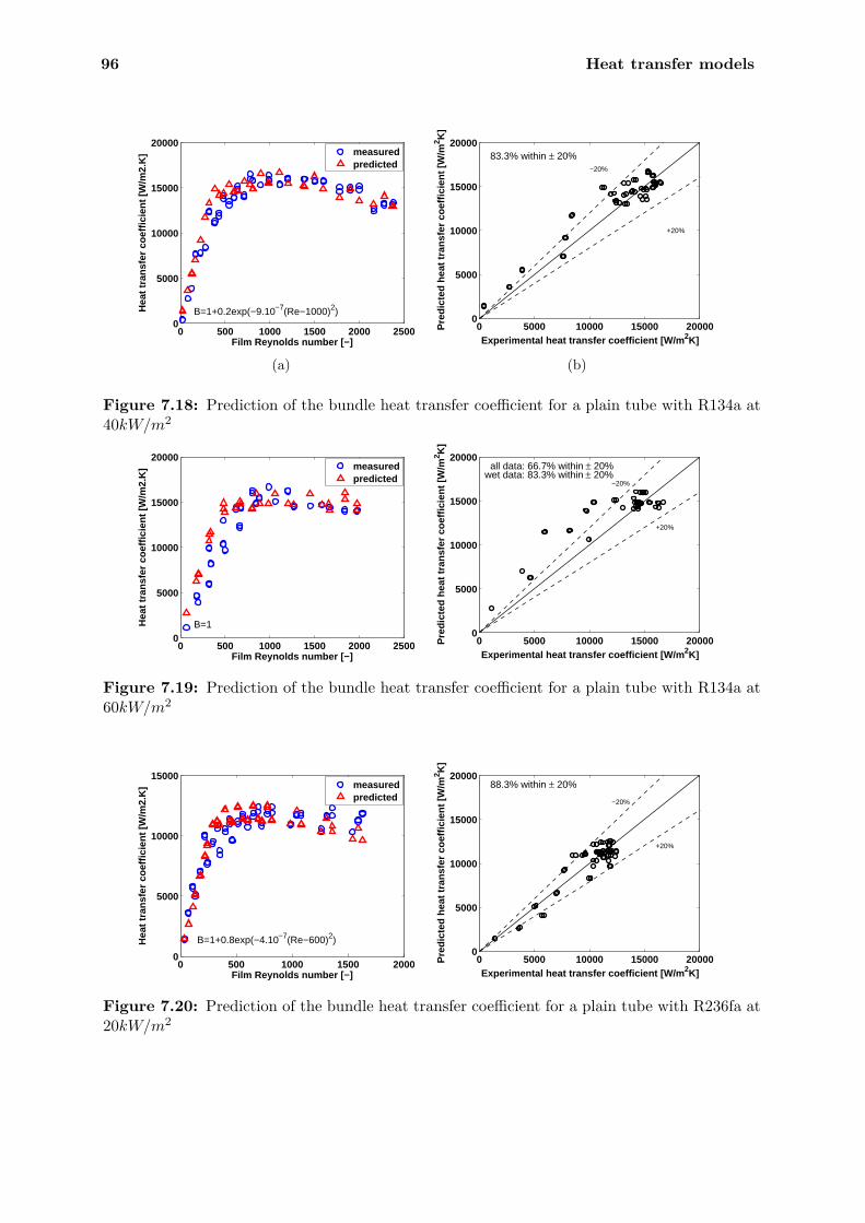
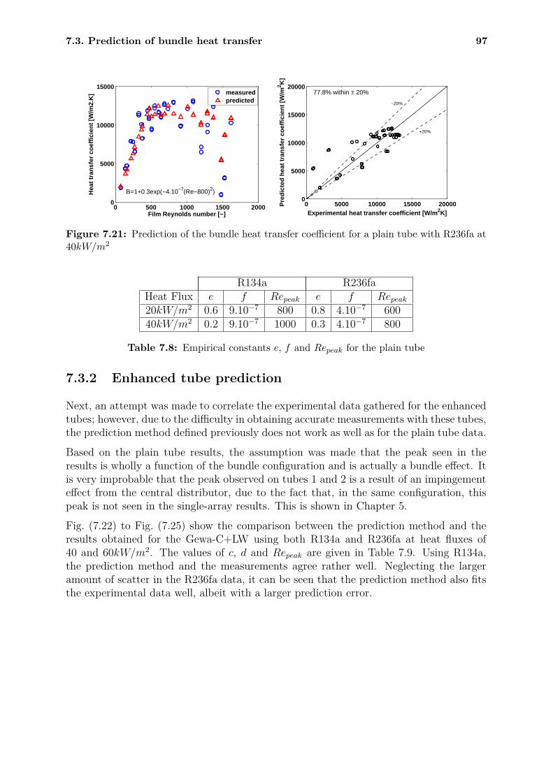
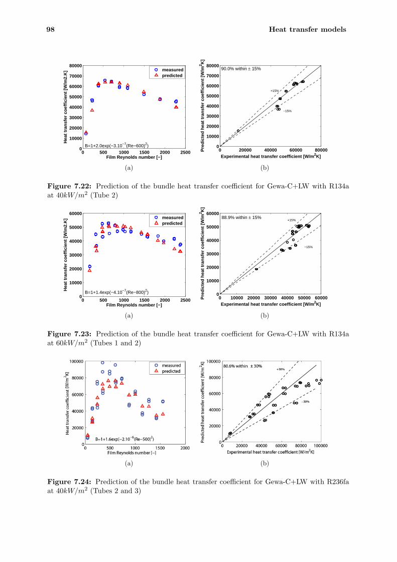
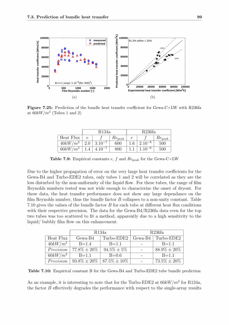


![Evaporation in a Binary Liquid Falling Film€¦ · In this report, we begin with the study of an isothermal 2-D falling film by Benney [8] in which effects from gravity, interfacial](https://static.documents.pub/doc/80x56/5ebef8f3aa3a7543ca4276f8/evaporation-in-a-binary-liquid-falling-film-in-this-report-we-begin-with-the-study.jpg)


