06-Mar-2017 Falling Film Reactor Master of Engineering Rianne Timmermans University of Groningen, Chemical Technology Tuinbouwdwarsstraat 23, 9717HT, Groningen +31644310064 [email protected]s2044706 First supervisor: prof. ir. M.W.M. Boesten [email protected]Second supervisor: prof. dr. F. Picchioni [email protected]A thesis submitted to the Department of Chemical Technology in partial fulfillment of the requirements for the degree of Master of Science in Chemical Engineering
Transcript
06-Mar-2017
Falling Film Reactor Master of Engineering
Rianne Timmermans University of Groningen, Chemical Technology Tuinbouwdwarsstraat 23, 9717HT, Groningen +31644310064 [email protected] s2044706
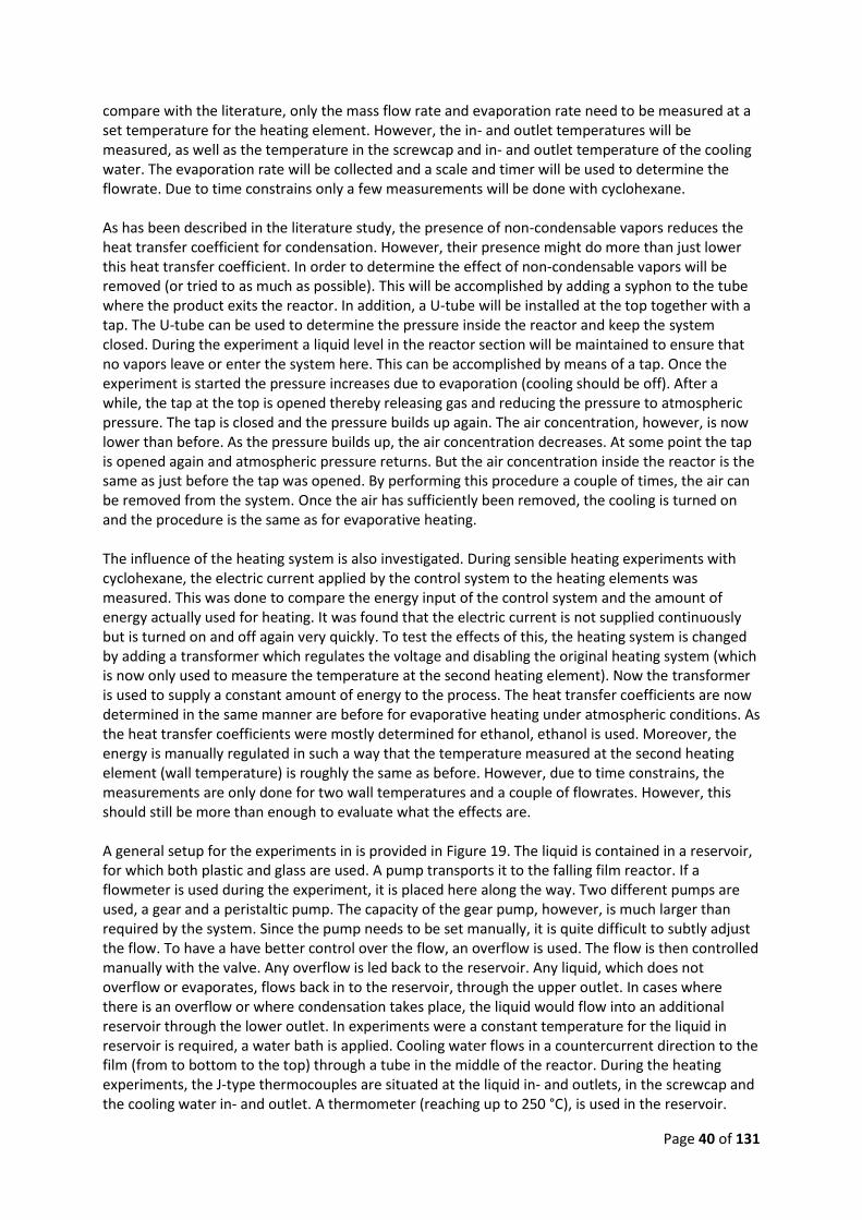
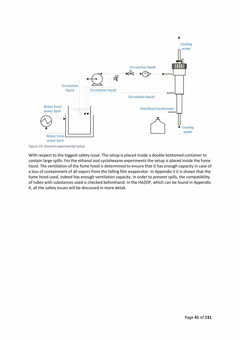
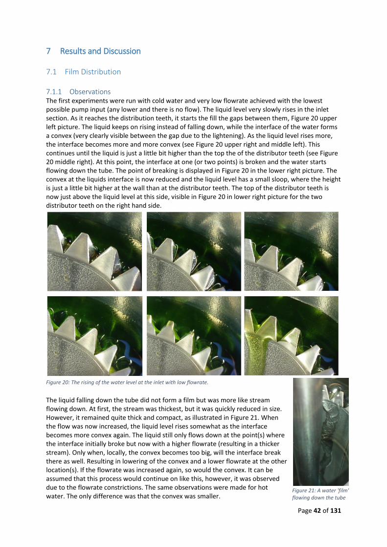
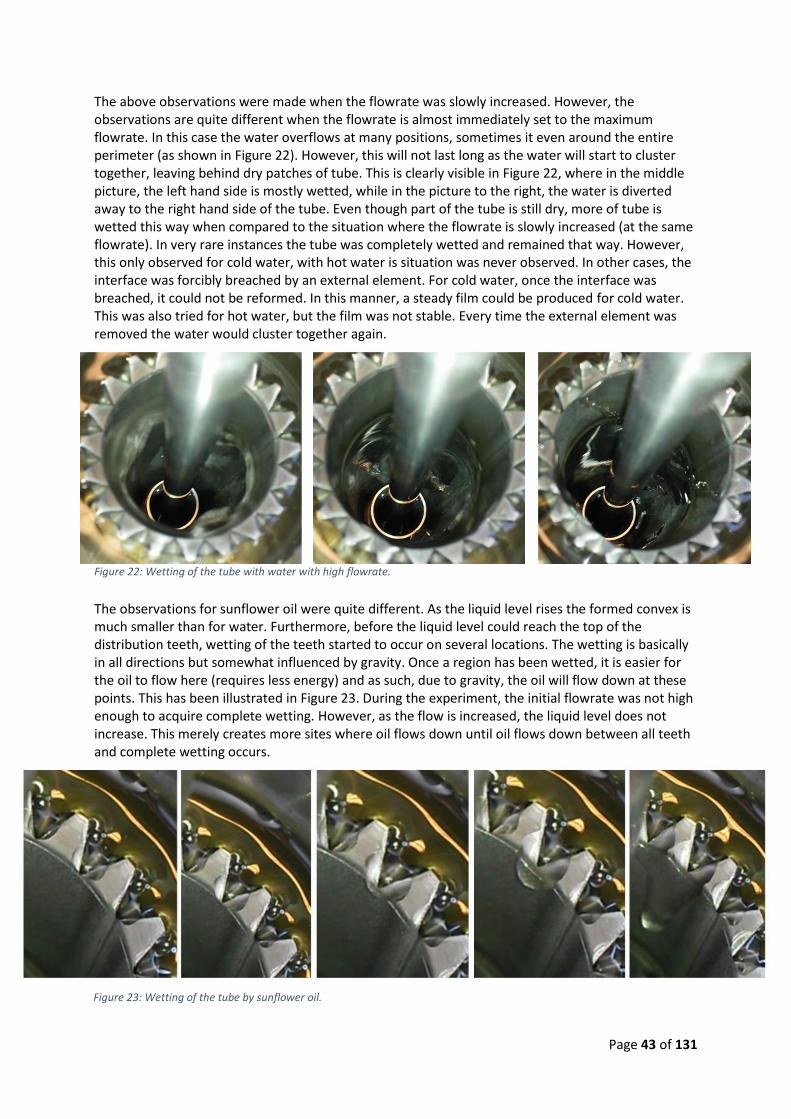
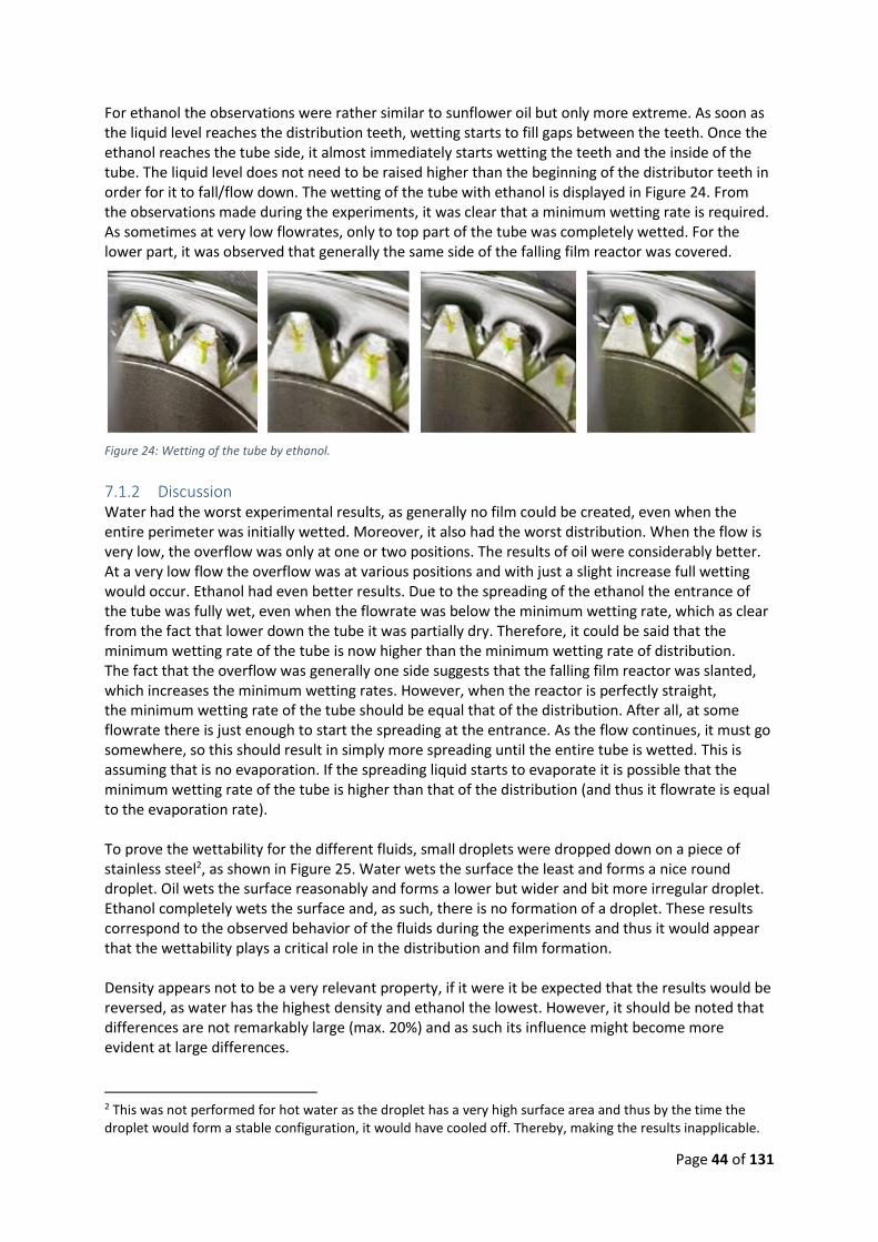
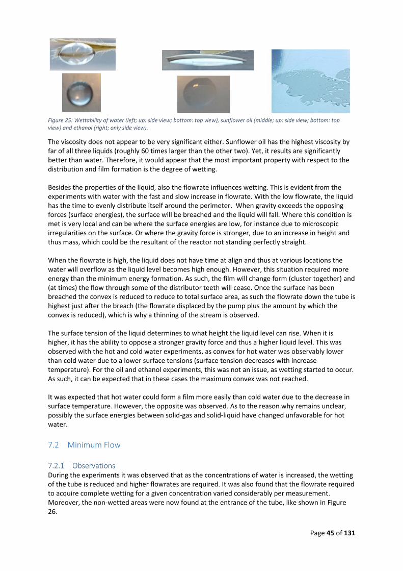
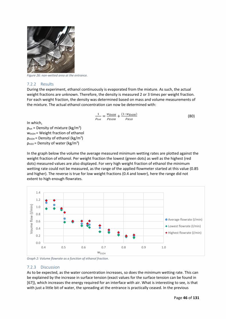
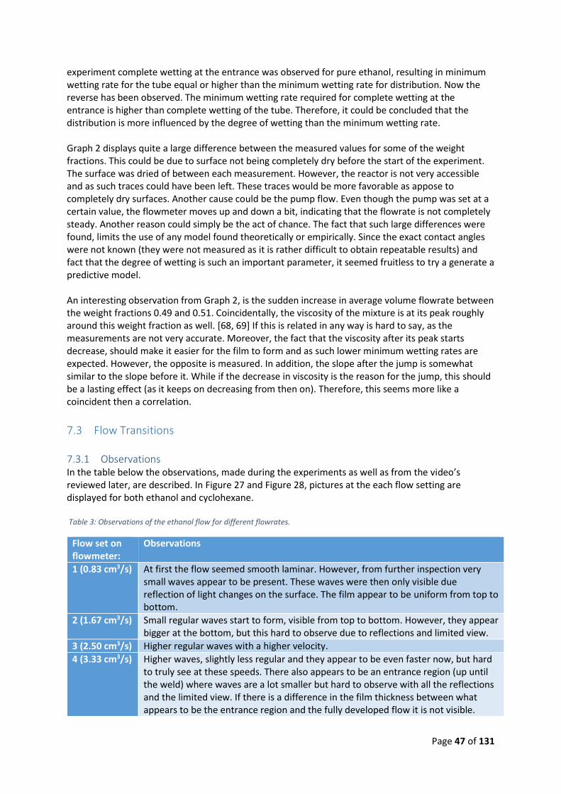
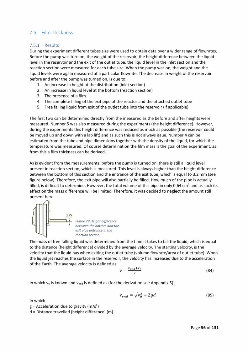
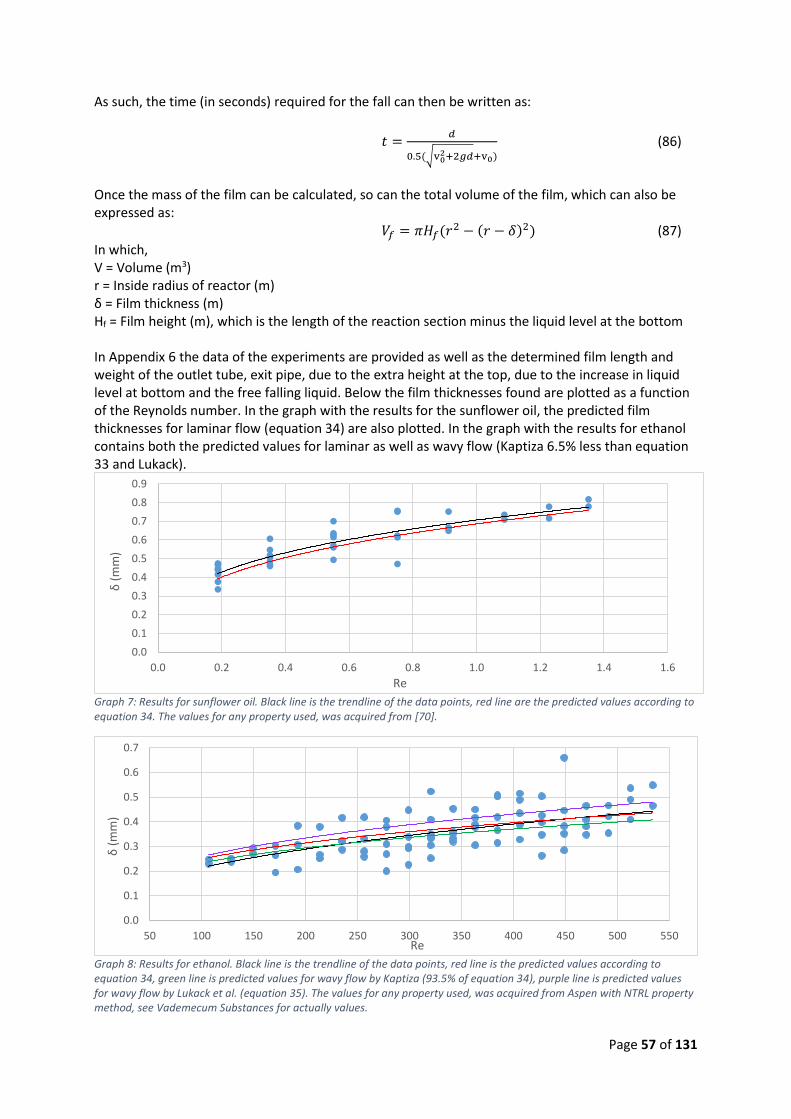
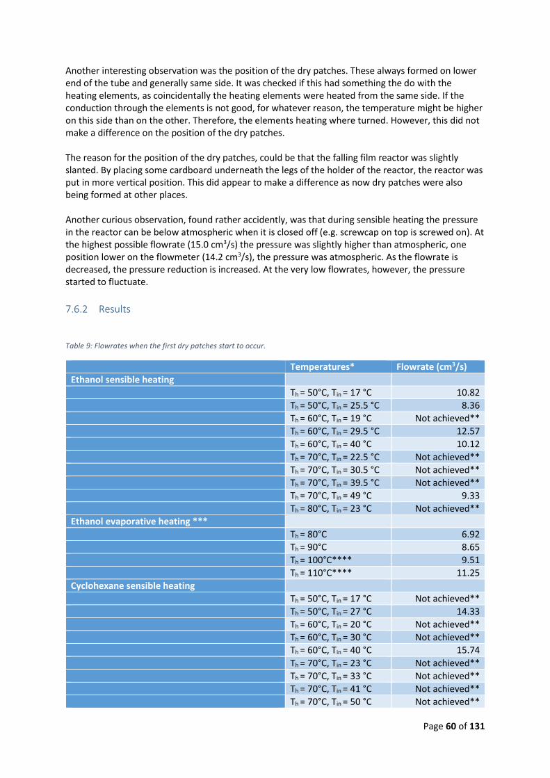
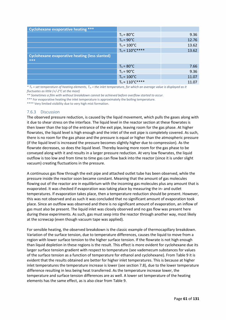
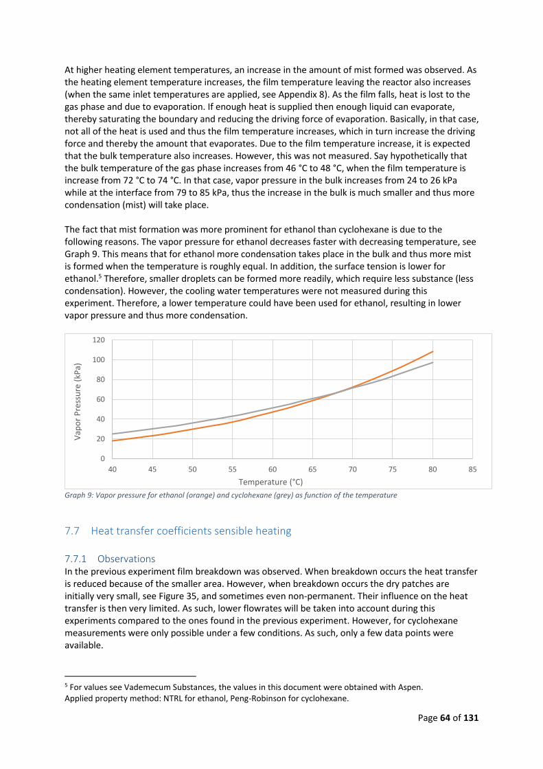
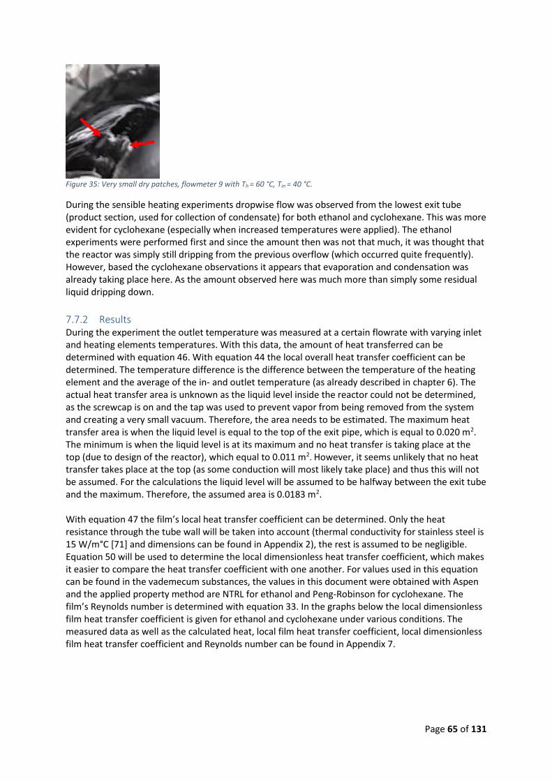
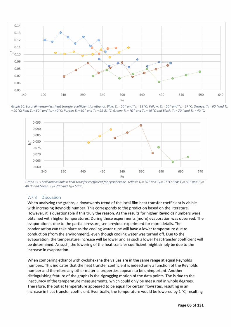
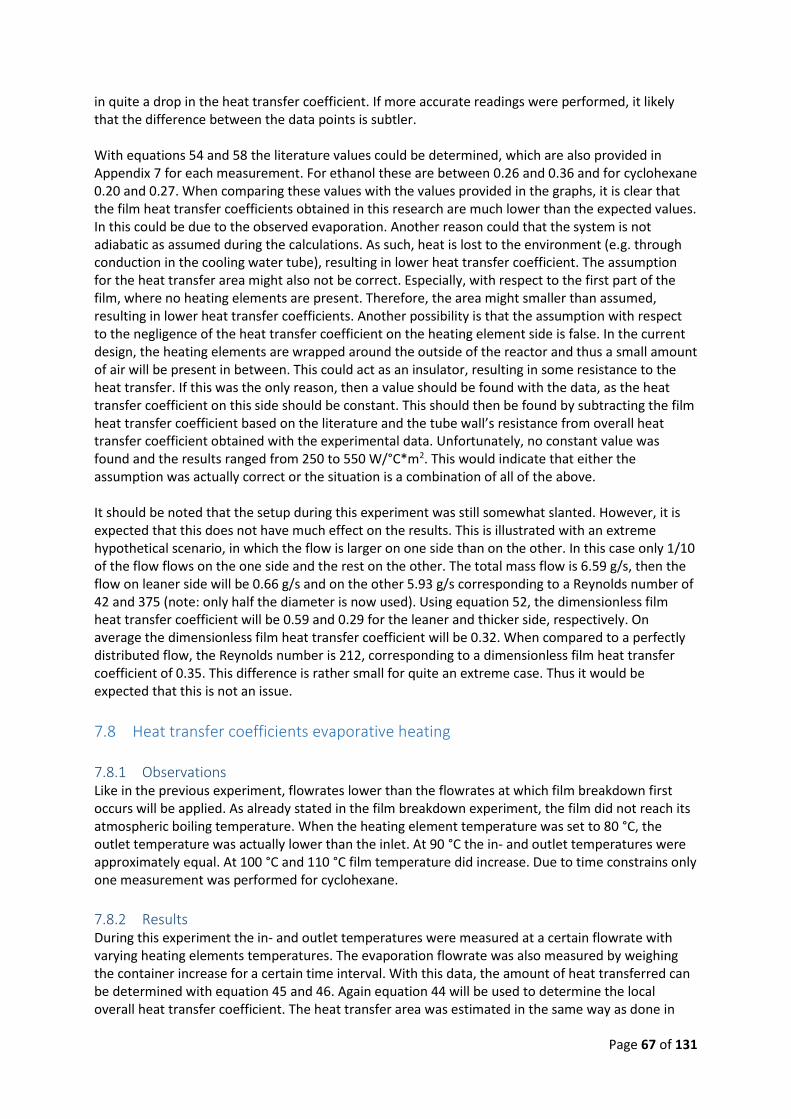
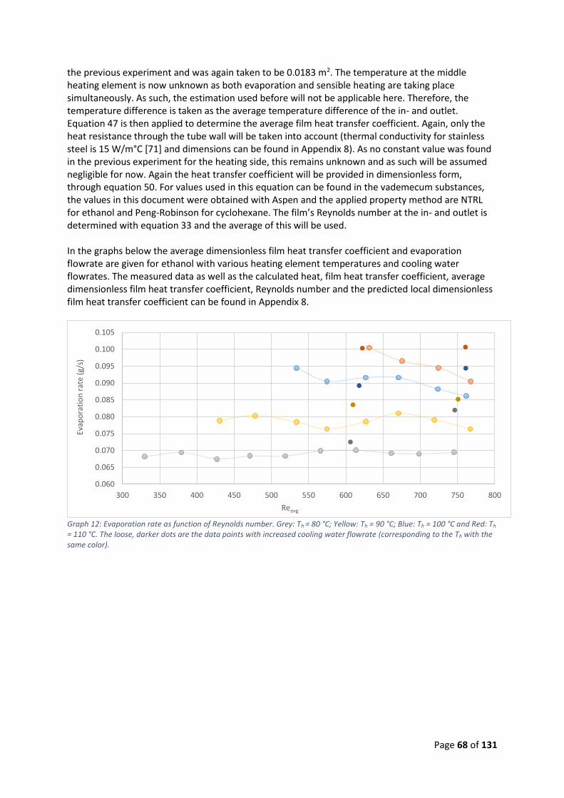
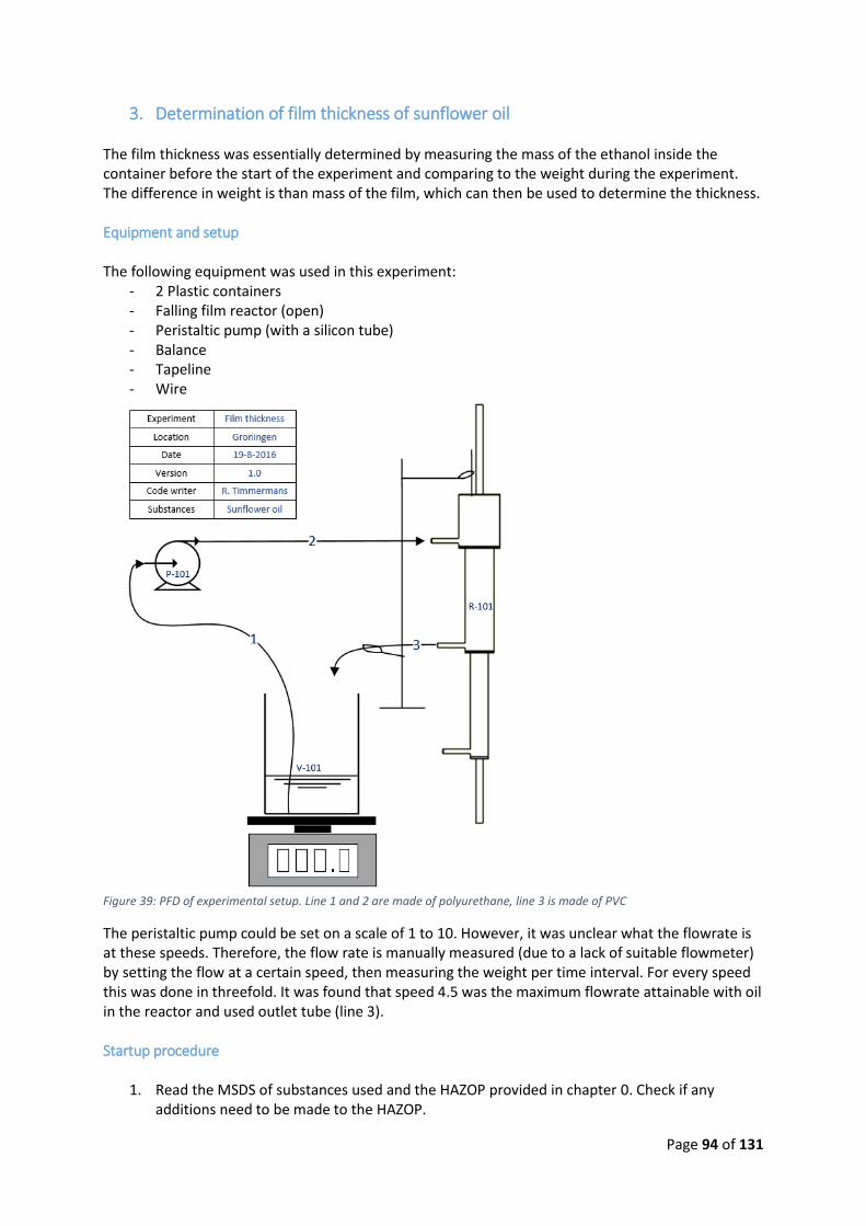
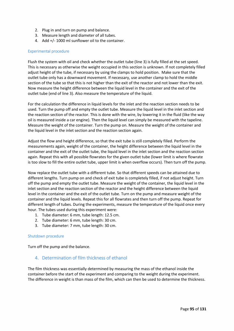
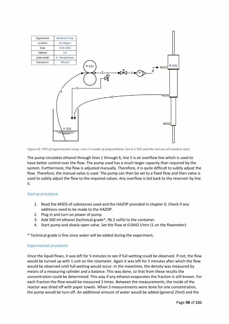
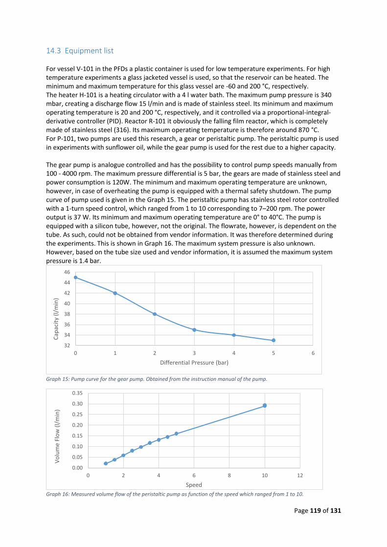
Abstract The falling film reactor, developed by the University of Groningen, is characterized with respect to its operating window. The University of Groningen initially developed the falling film reactor to perform more tests on the production of 1,4-butane diisocyanate (BDI) using short path distillation. The technology applied in this reactor is comparable to falling film evaporators and short path evaporators. However, compared to these evaporators, the design is quite different. First of all, the liquid distribution is completely different. Moreover, the cooling is performed internally while for falling film evaporators it is done externally. In addition, short path evaporators are generally operated at higher vacuums than required for the BDI production. Due to its unique design, it is unknown if the workings are similar to the current available designs and thus which theories are applicable. This study will provide some initial understanding of the falling film reactor. In the hope that it may someday not only be used in the production of BDI but possibly many other chemicals, which are currently not possible or profitable to be manufactured. The main conclusion of this research is that the concept of the falling film reactor works. However, as the experiments were performed in the presence of air, the obtained results were far below the predicted values based on the literature. The temperature of the liquid reservoir was kept at the atmospheric boiling temperature. However, the inlet temperature was lowered due to the cooling water through conduction. The pressure inside the reactor was maintained because of the presence of the air. As such, the liquid temperature is now below the boiling temperature. Evaporation is now determined by the difference between the partial pressure and equilibrium vapor pressure in the boundary layer, which lowers the evaporation rate when compared to a film at boiling temperature. As such, the heat transfer coefficient obtained in this research is much lower when compared to the predicted values. If enough heat is supplied, then the film temperature can increase along the tube length. Thereby increasing the driving force for evaporation resulting in a higher production. If the heat supplied is insufficient, then energy from bulk is used to accommodate the driving force, which lowers the film temperature and creating a constant production. By removing the non-condensable gases from the system, the liquid should always be at its boiling temperature and thus higher heat transfer coefficients should be found. It is therefore recommended that this matter is further investigated. The results for sensible heating were much better but still quite a bit lower than the predictions. This is in part due to evaporation and heat losses to the environment. However, it is also very likely that there is some heat resistance between the heating elements and the tube wall, which was assumed to be negligible. As such, these effects need to be further investigated. The observed film breakdown for both sensible and evaporative heating was due to thermocapillarity. As the film in neither situation was at its boiling temperature this was to be expected. Moreover, when the reactor was slanted, thermocapillary breakdown is enhanced. Therefore, to achieve optimal performance, it is essential that the reactor stands upright. For the liquid distribution, the most important parameter is the wettability. Although this is less important at higher flowrates. For the determination of the liquid level inside the reactor, the equations provided by the literature can quite accurately be used up to a mass flowrate of 3.5 g/s. The measured film thicknesses for laminar and wavy flow correspond quite nicely with the predictions. Thus the equations provided by the literature can be applied to this reactor. For both experiments, the measurements were not performed at higher flowrates, as such the equations for those flowrates provided by the literature still need to be verified.
14.3 Equipment list ...................................................................................................................... 119
15 Appendix 5: Derivation of the end velocity ............................................................................. 121
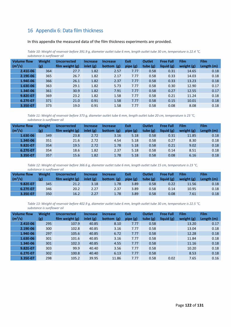
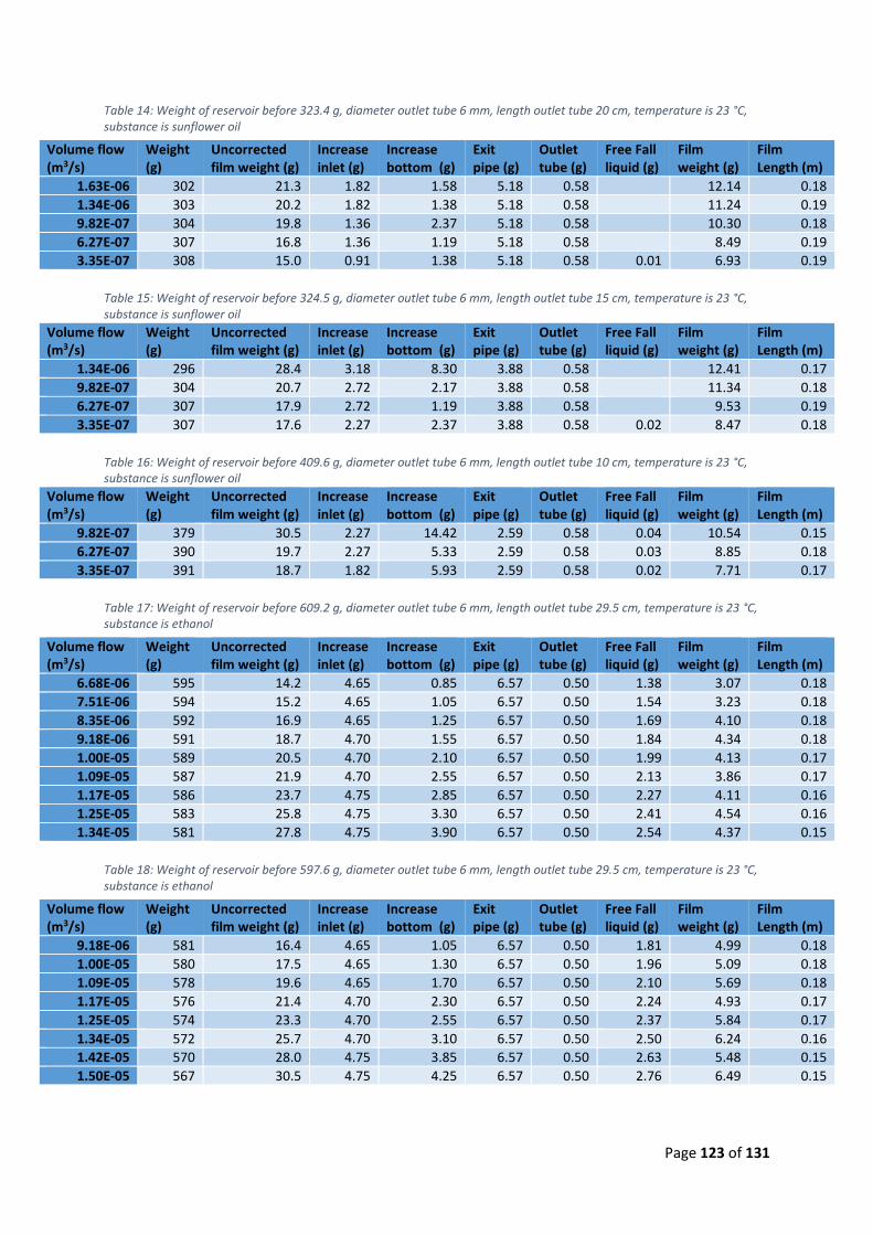
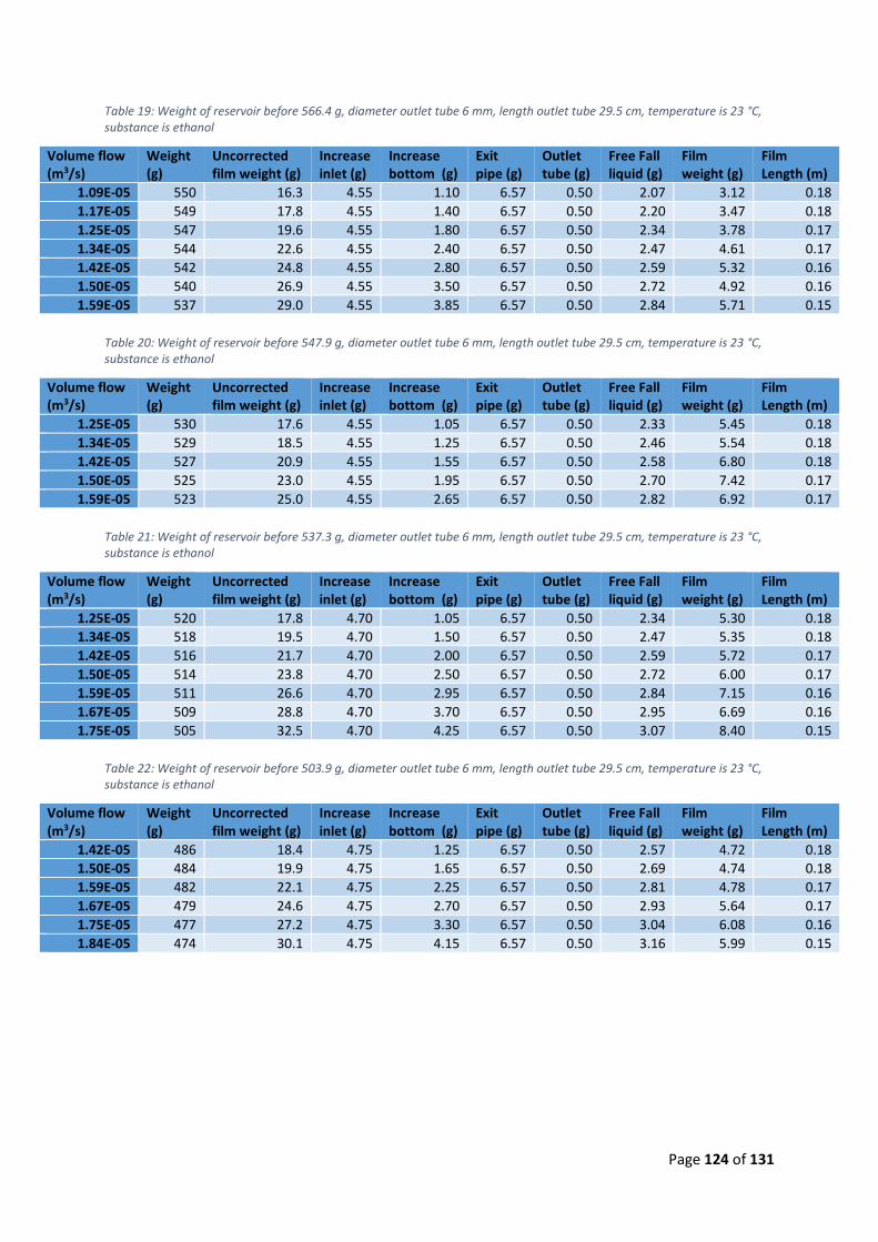
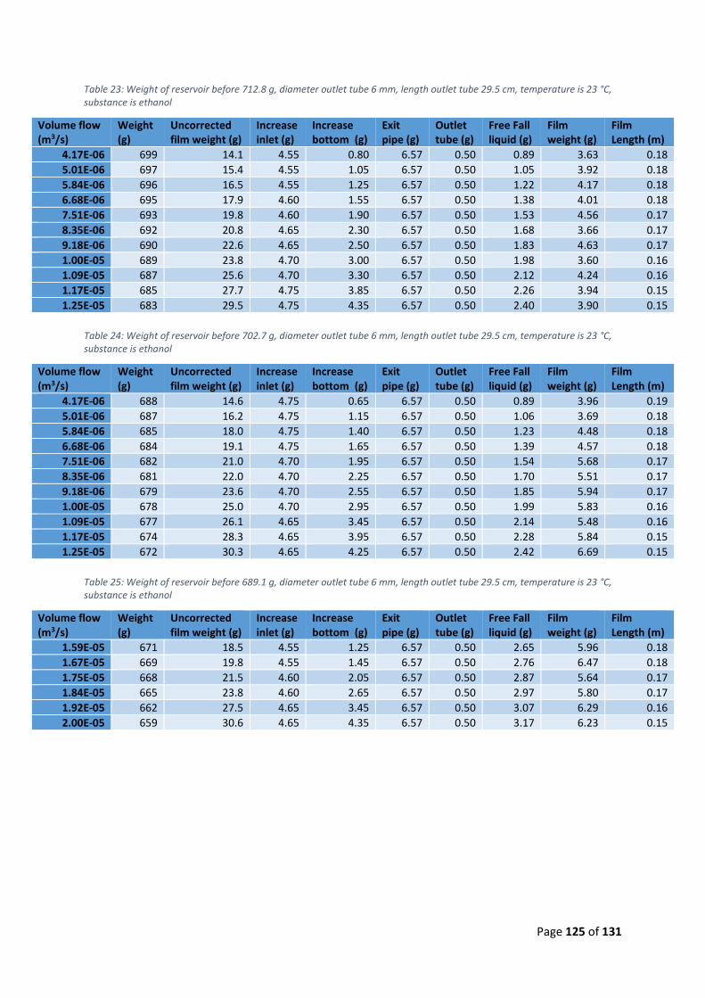
16 Appendix 6: Data film thickness .............................................................................................. 122
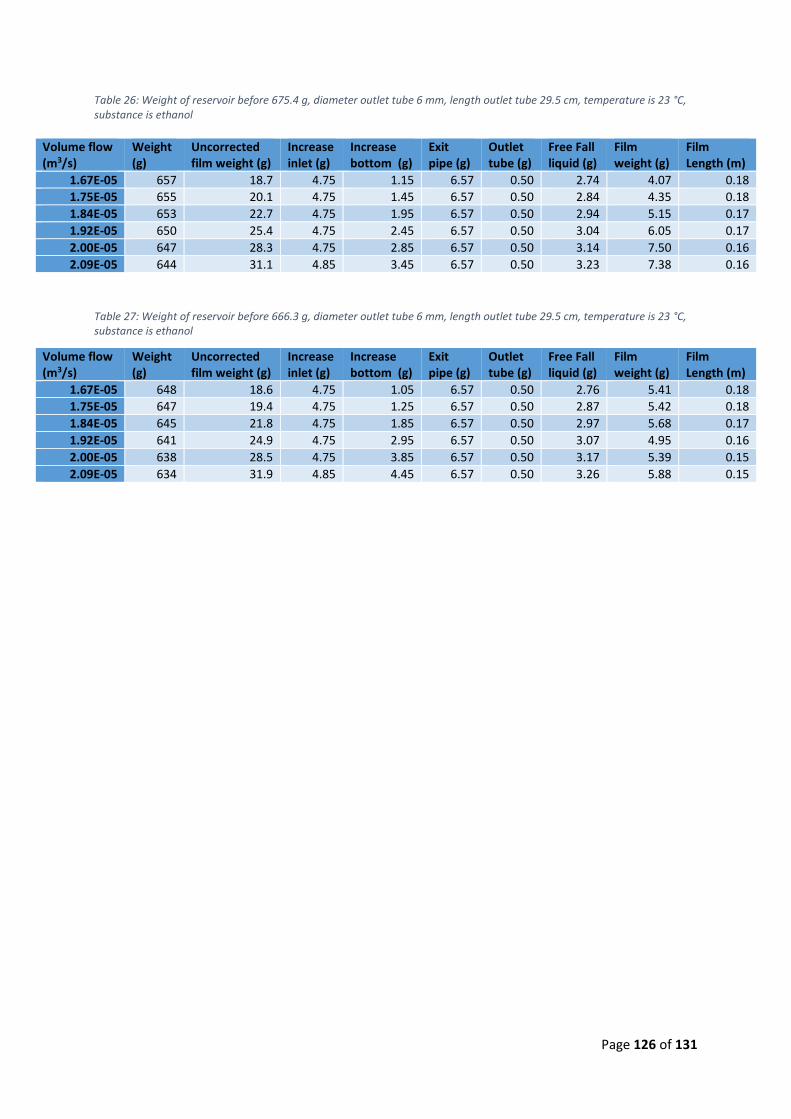
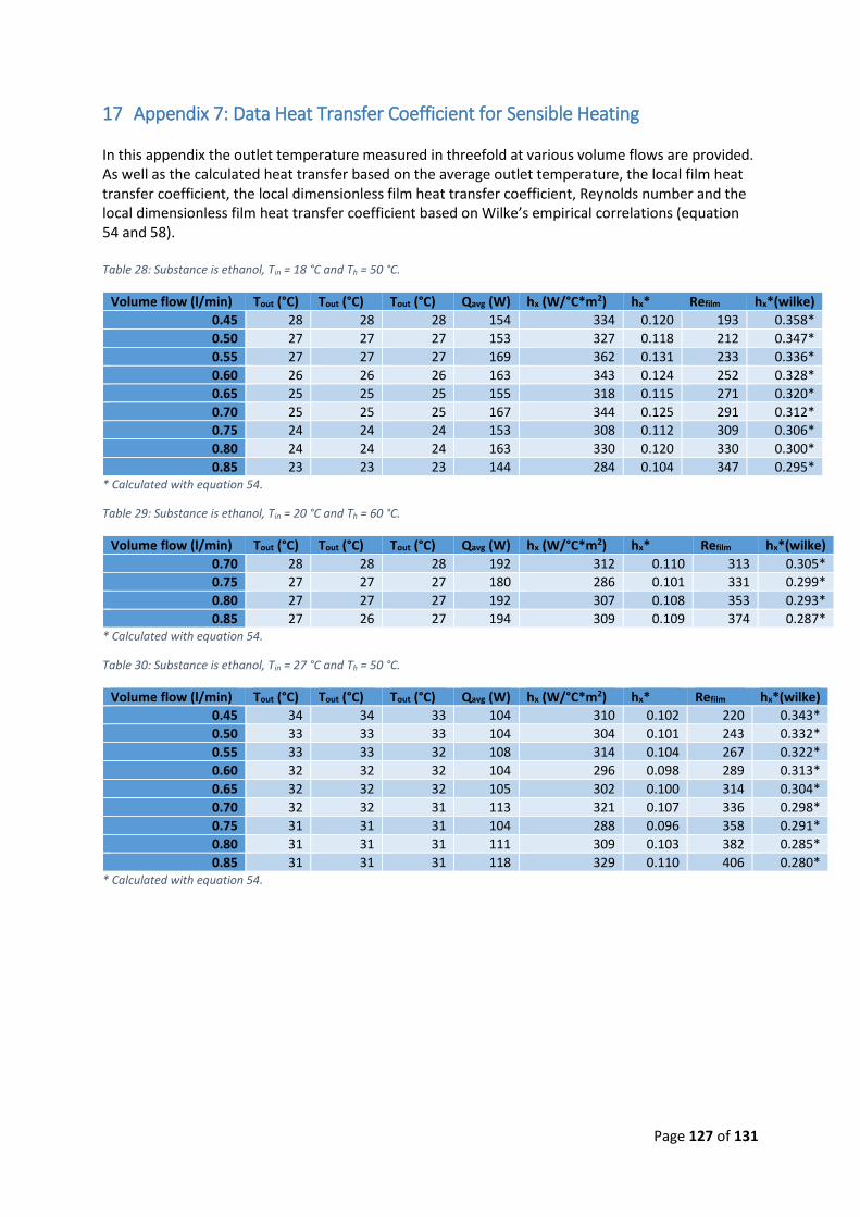
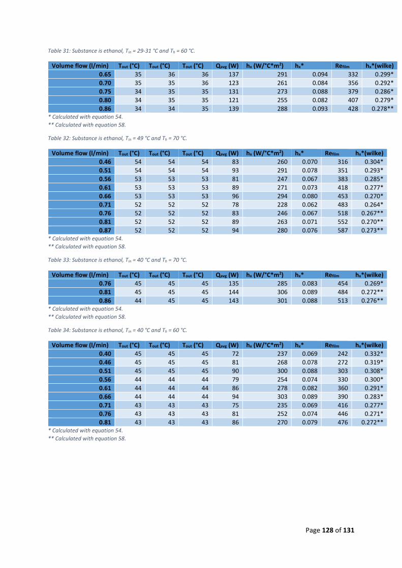
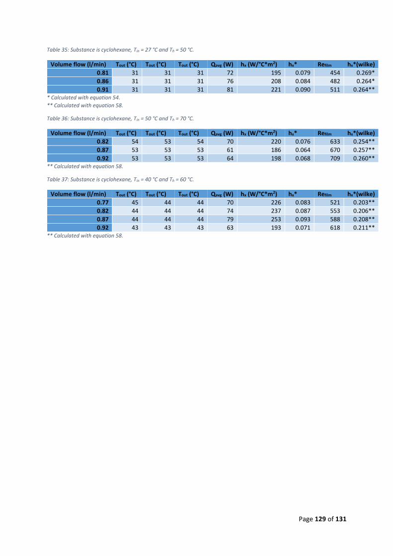
17 Appendix 7: Data Heat Transfer Coefficient for Sensible Heating .......................................... 127
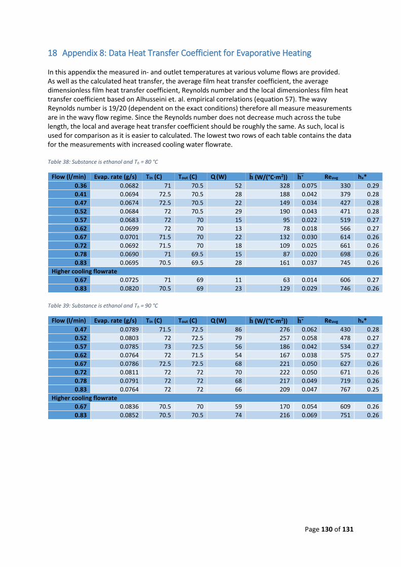
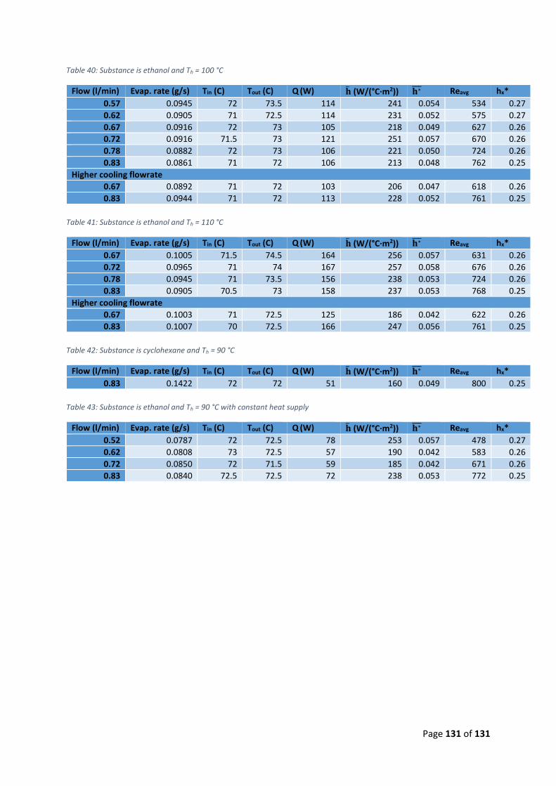
18 Appendix 8: Data Heat Transfer Coefficient for Evaporative Heating .................................... 130
Page 4 of 131
1 Nomenclature Ac Cross-sectional area m2 A = Heat transfer area m2 C and C’ Hagenbach and Couette corrections cp Specific heat capacity J/kg·°C Di Hydraulic diameter m D Diameter m e Tube wall thickness m g Acceleration due to gravity m/s2 H Height m ΔH Liquid level in evaporator m ΔHvap Enthalpy of vaporization J/kg ∆Hvap
∗ ‘Corrected’ enthalpy of vaporization J/kg
h Film heat transfer coefficient W/m2·°C ho Heat transfer coefficient on the outside of the tube W/m2·°C h* Dimensionless heat transfer coefficient -
ℎ∗ Average dimensionless heat transfer coefficient - K Loss coefficient - Lh Hydrodynamic entrance length m
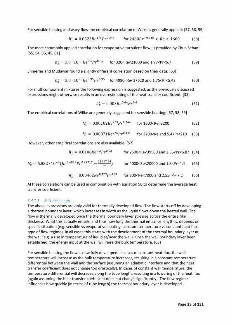
Lt Thermal entrance length m
Lf Film length m L Characteristic length m Ṁ Mass flow kg/s P Power supplied to or from system W p Pressure Pa ΔPent Pressure loss due to the contraction (entrance) Pa Q Heat transferred through the surface per unit time W q Heat flux W/m2 R Radius of tube m RF Fouling resistance m2·°C/W S Circumference of the area of the pipe m T Temperature °C ΔT Temperature difference wall and bulk of film °C T Time s U Overall heat transfer coefficient W/m2·°C V Volume m3
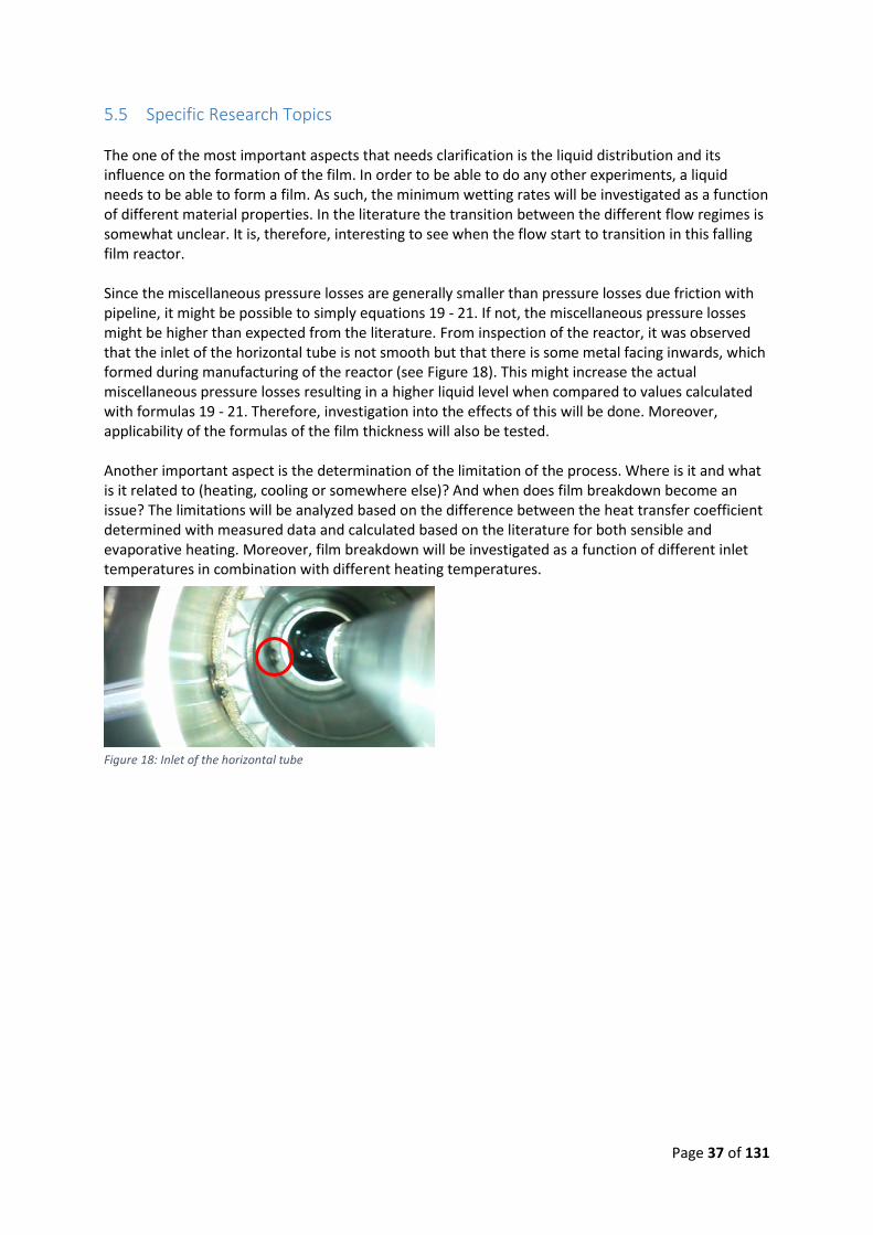
V Volume flow m3/s v Velocity m/s <v> Velocity averaged over the area m/s <vf> Mean velocity of film m/s w Weight fraction - x2-x1/x1-x3/ x3-x2 Length of the pipe m z Height difference between points 1 and 2 m Greek Symbols α constant depending on the expansion ratio β Area ratio (=D1
2/D22)
Γ Mass flowrate per unit perimeter kg/m·s δ Film thickness m
Page 5 of 131
ζ Friction coefficient - θ Contact angle ° λ Thermal conductivity W/m·°C μ Dynamic viscosity Pa·s 𝑣 Kinematic viscosity m2/s ρ Density kg/m3 σ Surface tension between liquid and vapor N/m Subscripts l Liquid g Gas v Vapor 0 Start 1 Point 1 in Figure 11 2 Point 2 in Figure 11 3 Point 3 in Figure 11 vap Evaporation sat Saturation f Film p Pipe x Local w Wall o Outside of the tube In Incoming film Out Outgoing film EtOH Ethanol H2O Water sun Sunflower oil fric Friction mics Miscellaneous m Logarithmic mean Dimensionless numbers
Re Reynolds number (=𝜌v𝐿
𝜇=
4𝛤
𝜇)
Pr Prandtl number (=cp·µ/λ)
Ka Kaptiza number (= 𝜌𝜎3
𝑔𝜇4)
Nu Nusselt number (h·L/λ)
Page 6 of 131
2 Introduction
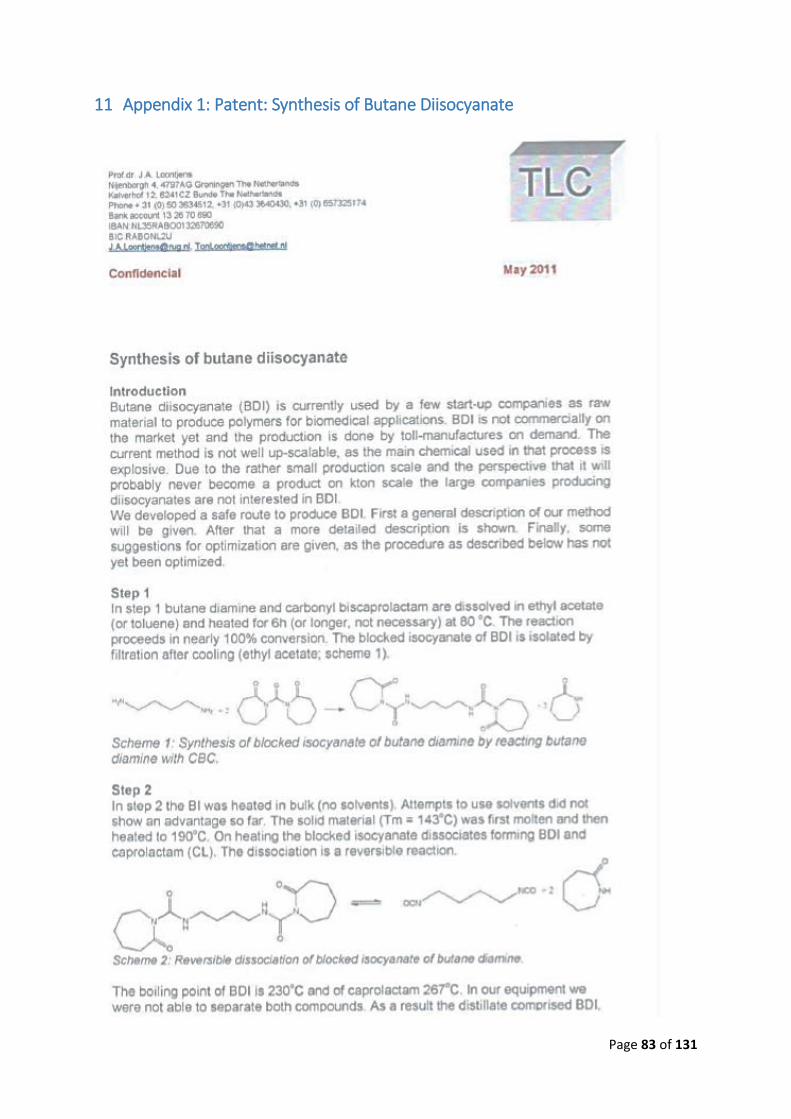
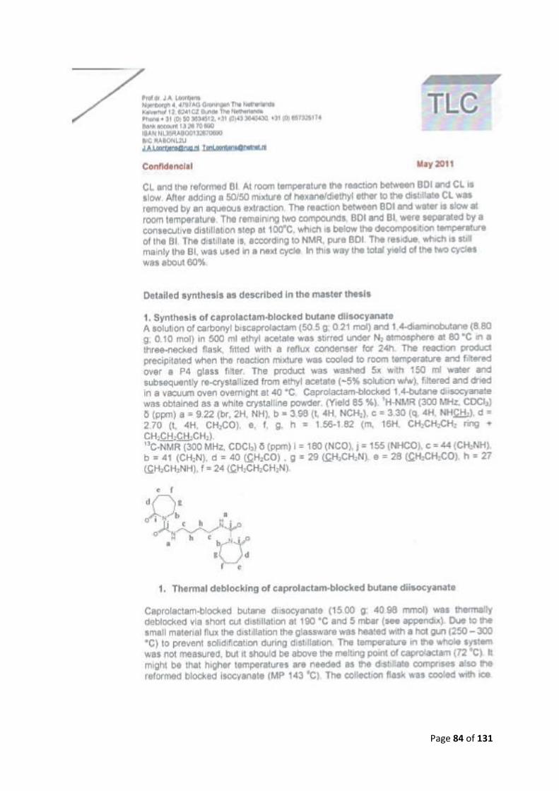
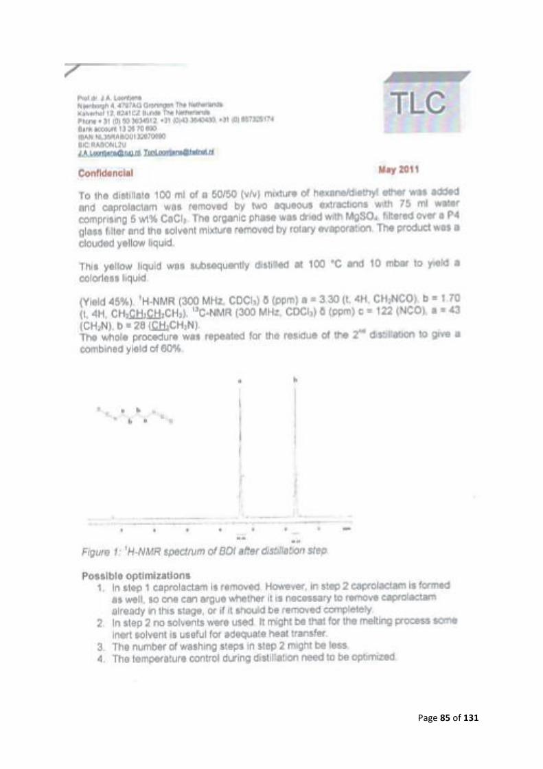
In this report the falling film reactor, developed by the University of Groningen, is characterized with respect to its operating window. The University of Groningen initially developed the falling film reactor to perform more tests on the production of 1,4-butane diisocyanate (BDI) using short path distillation. BDI can be used in the synthesis of polyurethanes that used to make porous 3D scaffolds, which are applied in tissue engineering. [1] However, the current production method of BDI is not suitable for large-scale. A different synthesis route has therefore been developed, which has shown success on lab scale (the patent can be found in Appendix 1). [2] This route synthesizes a blocked diisocyanate from carbonylbiscaprolactam and 1,4-butanediamine. The blocked diisocyanate is then disassociated, through the application of heat, into caprolactam and BDI. This reaction is an equilibrium reaction. One way to increase the BDI production is by removal of BDI from the mixture (LeChâtelier's Principle). Alas, during the lab experiments it was not possible to separate the compounds. This resulted in a distillate consisting of BDI, caprolactam and the blocked diisocyanate, which was created due to reverse reaction. However, the reverse reaction was observed to be slow at room temperature. [2] It is therefore essential to cool the distillate off as fast as possible to prevent the reverse reaction.
A suitable technique for large-scale production, which cools the distillate off quickly, is short-path distillation. A preliminary study has indeed shown that BDI can be synthesized with a wiped film evaporator. [3] To gain a better understanding into the production process and the factors influencing it, the University of Groningen has thus developed their own falling film reactor. Its design, however, is slightly different than the currently available falling film evaporators and short path evaporators (see section 2.2.2). Therefore, a deeper understanding of this unique falling film reactor is first required. This study aims to provide the first steps in understanding of this apparatus. Furthermore, it is hoped that the knowledge gained about this reactor can someday be used for the manufacturing of chemicals that are currently not possible or unprofitable.
2.1 Description of the falling film reactor
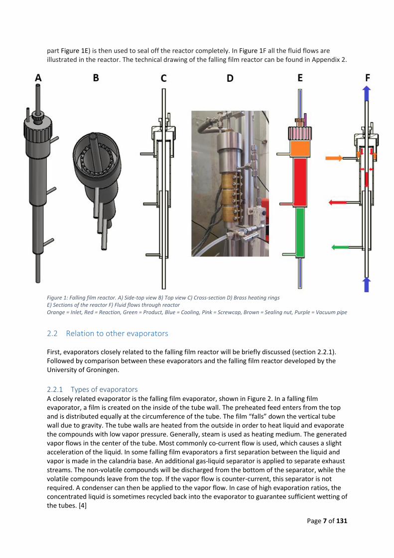
The falling film reactor developed by the University of Groningen basically consists of multiple tubes with different lengths and diameters welded together, as shown in Figure 1. Based on function, different sections can be identified. First the feed enters the reactor through small horizontal pipe, where it is collected in the inlet section (orange part Figure 1E). When starting up, the liquid level in the inlet section will rise if enough pressure is available to overcome height difference. This will continue up until distributor teeth. Here the liquid will fill the gaps between the teeth. Due to gravity, the liquid will fall down along the inner wall of the tube, creating a uniform distributed film and entering the reaction section (red part Figure 1E). In the reaction section the tube wall is heated from the outside through three brass rings (see Figure 1D). The brass rings are electronically heated through a temperature controller. The heat is then transferred to the film, which will cause heating of the film, leading to (faster) reactions or decompositions, or, if already at sufficient temperature, evaporation (of volatile components). The film will not completely be evaporated, this ‘leftover’ film will leave the reactor at the bottom of the reactor section through a small horizontal pipe (equal in size to the inlet pipe). The vapor will move to the center of the tube, where it is condensed on the outside of the cooling pipe (blue part Figure 1E). The condensed vapor will flow down on the outside of this pipe due to gravity into the product section (green part Figure 1E). There it will leave the reactor through the small horizontal pipe (equal in size to the inlet and other outlet pipe). A cooling medium, such tab water, will flow through the cooling tube. To close the reactor a screwcap can be used to close off the inlet section. On this screwcap another small pipe (purple part Figure 1E) has been mounted to be able to apply a vacuum (or high pressure) to the reactor. A sealing nut (brown
Page 7 of 131
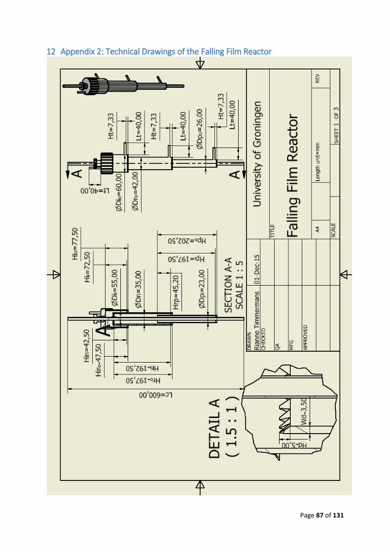
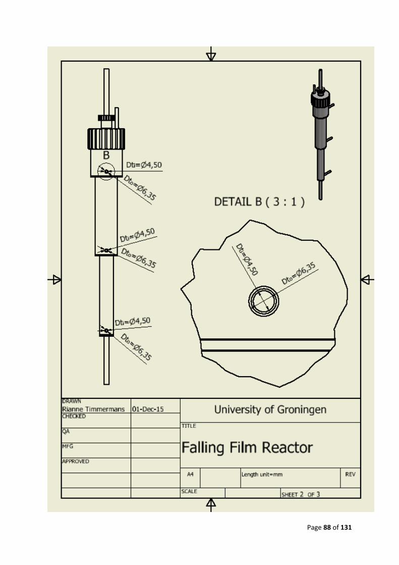
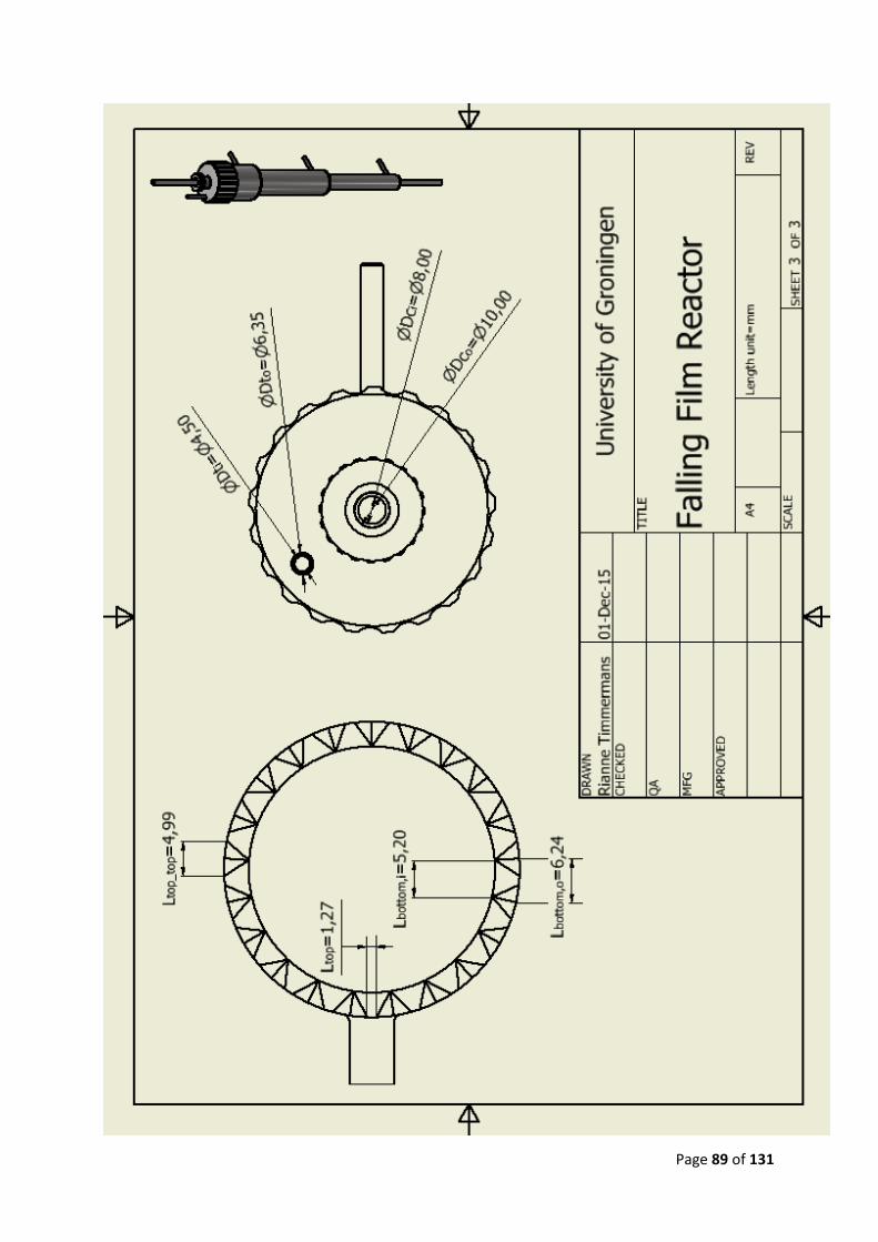
part Figure 1E) is then used to seal off the reactor completely. In Figure 1F all the fluid flows are illustrated in the reactor. The technical drawing of the falling film reactor can be found in Appendix 2.
2.2 Relation to other evaporators First, evaporators closely related to the falling film reactor will be briefly discussed (section 2.2.1). Followed by comparison between these evaporators and the falling film reactor developed by the University of Groningen.
2.2.1 Types of evaporators A closely related evaporator is the falling film evaporator, shown in Figure 2. In a falling film evaporator, a film is created on the inside of the tube wall. The preheated feed enters from the top and is distributed equally at the circumference of the tube. The film “falls” down the vertical tube wall due to gravity. The tube walls are heated from the outside in order to heat liquid and evaporate the compounds with low vapor pressure. Generally, steam is used as heating medium. The generated vapor flows in the center of the tube. Most commonly co-current flow is used, which causes a slight acceleration of the liquid. In some falling film evaporators a first separation between the liquid and vapor is made in the calandria base. An additional gas-liquid separator is applied to separate exhaust streams. The non-volatile compounds will be discharged from the bottom of the separator, while the volatile compounds leave from the top. If the vapor flow is counter-current, this separator is not required. A condenser can then be applied to the vapor flow. In case of high evaporation ratios, the concentrated liquid is sometimes recycled back into the evaporator to guarantee sufficient wetting of the tubes. [4]
Figure 1: Falling film reactor. A) Side-top view B) Top view C) Cross-section D) Brass heating rings E) Sections of the reactor F) Fluid flows through reactor Orange = Inlet, Red = Reaction, Green = Product, Blue = Cooling, Pink = Screwcap, Brown = Sealing nut, Purple = Vacuum pipe
Page 8 of 131
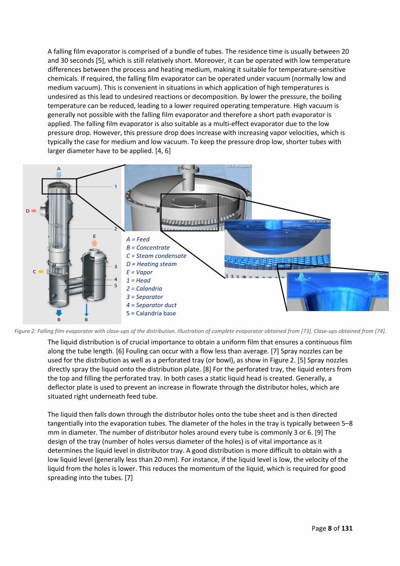
A falling film evaporator is comprised of a bundle of tubes. The residence time is usually between 20 and 30 seconds [5], which is still relatively short. Moreover, it can be operated with low temperature differences between the process and heating medium, making it suitable for temperature-sensitive chemicals. If required, the falling film evaporator can be operated under vacuum (normally low and medium vacuum). This is convenient in situations in which application of high temperatures is undesired as this lead to undesired reactions or decomposition. By lower the pressure, the boiling temperature can be reduced, leading to a lower required operating temperature. High vacuum is generally not possible with the falling film evaporator and therefore a short path evaporator is applied. The falling film evaporator is also suitable as a multi-effect evaporator due to the low pressure drop. However, this pressure drop does increase with increasing vapor velocities, which is typically the case for medium and low vacuum. To keep the pressure drop low, shorter tubes with larger diameter have to be applied. [4, 6]
The liquid distribution is of crucial importance to obtain a uniform film that ensures a continuous film along the tube length. [6] Fouling can occur with a flow less than average. [7] Spray nozzles can be used for the distribution as well as a perforated tray (or bowl), as show in Figure 2. [5] Spray nozzles directly spray the liquid onto the distribution plate. [8] For the perforated tray, the liquid enters from the top and filling the perforated tray. In both cases a static liquid head is created. Generally, a deflector plate is used to prevent an increase in flowrate through the distributor holes, which are situated right underneath feed tube. The liquid then falls down through the distributor holes onto the tube sheet and is then directed tangentially into the evaporation tubes. The diameter of the holes in the tray is typically between 5–8 mm in diameter. The number of distributor holes around every tube is commonly 3 or 6. [9] The design of the tray (number of holes versus diameter of the holes) is of vital importance as it determines the liquid level in distributor tray. A good distribution is more difficult to obtain with a low liquid level (generally less than 20 mm). For instance, if the liquid level is low, the velocity of the liquid from the holes is lower. This reduces the momentum of the liquid, which is required for good spreading into the tubes. [7]
Figure 2: Falling film evaporator with close-ups of the distribution. Illustration of complete evaporator obtained from [73]. Close-ups obtained from [74].
A = Feed
B = Concentrate
C = Steam condensate D = Heating steam E = Vapor 1 = Head
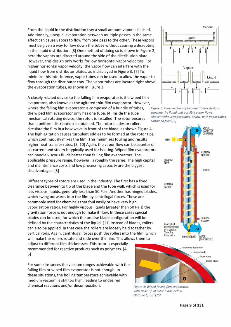
From the liquid in the distribution tray a small amount vapor is flashed. Additionally, unequal evaporation between multiple passes in the same effect can cause vapors to flow from one pass to the other. These vapors must be given a way to flow down the tubes without causing a disrupting in the liquid distribution. [8] One method of doing so is shown in Figure 2, here the vapors are directed around the side of the distribution plate. However, this design only works for low horizontal vapor velocities. For higher horizontal vapor velocity, the vapor flow can interfere with the liquid flow from distributor plates, as is displayed in Figure 3. [7] To minimize this interference, vapor tubes can be used to allow the vapor to flow through the distributor tray. The vapor tubes are located right above the evaporation tubes, as shown in Figure 3. A closely related device to the falling film evaporator is the wiped film evaporator, also known as the agitated thin-film evaporator. However, where the falling film evaporator is composed of a bundle of tubes, the wiped film evaporator only has one tube. [4] Inside the tube mechanical rotating device, the rotor, is installed. The rotor ensures that a uniform distribution is obtained. The rotor blades or rollers circulate the film in a bow wave in front of the blade, as shown Figure 4. The high agitation causes turbulent eddies to be formed at the rotor tips, which continuously mixes the film. This minimizes fouling and results higher heat transfer rates. [5, 10] Again, the vapor flow can be counter or co-current and steam is typically used for heating. Wiped film evaporators can handle viscous fluids better than falling film evaporators. The applicable pressure range, however, is roughly the same. The high capital and maintenance costs and low processing capacity are the biggest disadvantages. [5] Different types of rotors are used in the industry. The first has a fixed clearance between to tip of the blade and the tube wall, which is used for less viscous liquids, generally less than 50 Pa·s. Another has hinged blades, which swing outwards into the film by centrifugal forces. These are commonly used for chemicals that foul easily or have very high vaporization ratios. For highly viscous liquids (greater than 50 Pa·s) the gravitation force is not enough to make it flow. In these cases special blades can be used, for which the precise blade configuration will be defined by the characteristics of the liquid. [11] Instead of blades, rollers can also be applied. In that case the rollers are loosely held together by vertical rods. Again, centrifugal forces push the rollers into the film, which will make the rollers rotate and slide over the film. This allows them to adjust to different film thicknesses. This rotor is especially recommended for reactive products such as polymers. [4, 6] For some instances the vacuum ranges achievable with the falling film or wiped film evaporator is not enough. In these situations, the boiling temperature achievable with medium vacuum is still too high, leading to undesired chemical reactions and/or decomposition.
Figure 3: Cross-section of two distributor designs showing the liquid and possible vapor flows: Above: without vapor tubes. Below: with vapor tubes. Obtained from [7]
Figure 4: Wiped falling film evaporator, with close-up of rotor blade below. Obtained from [75]
Page 10 of 131
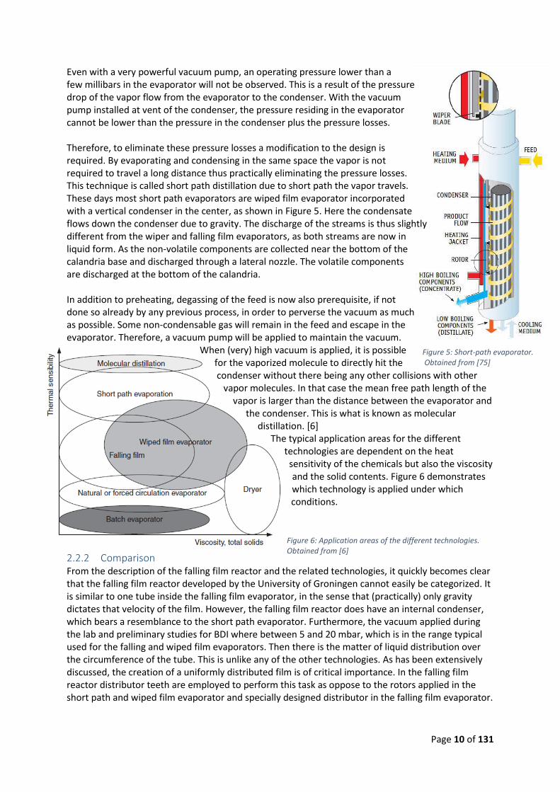
Even with a very powerful vacuum pump, an operating pressure lower than a few millibars in the evaporator will not be observed. This is a result of the pressure drop of the vapor flow from the evaporator to the condenser. With the vacuum pump installed at vent of the condenser, the pressure residing in the evaporator cannot be lower than the pressure in the condenser plus the pressure losses. Therefore, to eliminate these pressure losses a modification to the design is required. By evaporating and condensing in the same space the vapor is not required to travel a long distance thus practically eliminating the pressure losses. This technique is called short path distillation due to short path the vapor travels. These days most short path evaporators are wiped film evaporator incorporated with a vertical condenser in the center, as shown in Figure 5. Here the condensate flows down the condenser due to gravity. The discharge of the streams is thus slightly different from the wiper and falling film evaporators, as both streams are now in liquid form. As the non-volatile components are collected near the bottom of the calandria base and discharged through a lateral nozzle. The volatile components are discharged at the bottom of the calandria. In addition to preheating, degassing of the feed is now also prerequisite, if not done so already by any previous process, in order to perverse the vacuum as much as possible. Some non-condensable gas will remain in the feed and escape in the evaporator. Therefore, a vacuum pump will be applied to maintain the vacuum.
When (very) high vacuum is applied, it is possible for the vaporized molecule to directly hit the condenser without there being any other collisions with other
vapor molecules. In that case the mean free path length of the vapor is larger than the distance between the evaporator and
the condenser. This is what is known as molecular distillation. [6]
The typical application areas for the different technologies are dependent on the heat
sensitivity of the chemicals but also the viscosity and the solid contents. Figure 6 demonstrates which technology is applied under which conditions.
2.2.2 Comparison From the description of the falling film reactor and the related technologies, it quickly becomes clear that the falling film reactor developed by the University of Groningen cannot easily be categorized. It is similar to one tube inside the falling film evaporator, in the sense that (practically) only gravity dictates that velocity of the film. However, the falling film reactor does have an internal condenser, which bears a resemblance to the short path evaporator. Furthermore, the vacuum applied during the lab and preliminary studies for BDI where between 5 and 20 mbar, which is in the range typical used for the falling and wiped film evaporators. Then there is the matter of liquid distribution over the circumference of the tube. This is unlike any of the other technologies. As has been extensively discussed, the creation of a uniformly distributed film is of critical importance. In the falling film reactor distributor teeth are employed to perform this task as oppose to the rotors applied in the short path and wiped film evaporator and specially designed distributor in the falling film evaporator.
Figure 6: Application areas of the different technologies. Obtained from [6]
Figure 5: Short-path evaporator. Obtained from [75]
Page 11 of 131
3 Background information The aim of tissue engineering is regenerating damaged human tissue instead replacing it by other tissue through transplantation. For this biological substitutes are developed which can restore, maintain or improve tissue function. These biological substitutes are created from porous 3D scaffolds, which act as a template for tissue formation. The scaffolds are generally seeded with cells and on occasion growth factors and can be applied in vitro or in vivo. Biomaterials suitable for scaffold production must be: [12, 13]
- Biocompatible (cell adherence and no severe inflammatory response) - Biodegradable (degradation products should be non-toxic) - Suitable mechanical properties (allow surgical handling during implantation) - Scaffold architecture (have an interconnected pore structure and high porosity) - Manufacturing technology (should be cost effective and suitable for large-scale production)
Biodegradable polymers are the most promising biomaterials and, in particular, polyurethanes seem to be attractive candidates. Apart from being able to be biocompatible, they can have excellent mechanical properties and mechanical flexibility. [1] Furthermore, they can be biodegradable as the ester and ether groups can degrade through hydrolysis in vivo. [13] Aliphatic or cyclic diisocyanates are employed as their degradation products are less likely to be toxic as appose to aromatic diisocyanates, because they are known to degrade into carcinogenic and mutagenic aromatic amines. [1, 13] One of such an aliphatic diisocyanate is 1,4-butane diisocyanate. However, BDI is currently not produced commercially and is only produced on demand by toll-manufacturers. Furthermore, the production method employed is not suitable for large-scale since the main compound used in the process is explosive. Therefore, a different synthesis route has been developed. This route consists of carbonylbiscaprolactam reacting with 1,4-butanediamine creating a blocked diisocyanate and caprolactam. These two are then separated and the blocked diisocyanate is subsequently disassociated into BDI and caprolactam. [2] The disassociation reaction of the blocked diisocyanate is an equilibrium reaction [2] and thus a mixture of the blocked diisocyanate, caprolactam and BDI will be formed. The ratios of the chemicals are dependent on the conditions (e.g. temperature, pressure etc.). One way to increase the production of BDI is by favorably changing these conditions. Another way to favorably shift the equilibrium is by removing BDI from the mixture. On an industrial scale, a film evaporator, or more accurately a film reactor, is a possible technology to perform the reaction and shift the equilibrium to the product side. A previous study has concluded that the production of BDI using a film reactor is possible. [3] However, these results were only preliminary and left various questions unanswered. In order to learn more about this process, find the optimal process conditions and determine whether it is suitable for large-scale, the University of Groningen has developed a falling film reactor of their own. However, due to its unique design, it is unknown if the workings of this falling film reactor is similar to the falling film evaporator and if so, which theories are applicable. This study is to provide some initial understanding of the falling film reactor. In the hope that it may someday not only be used in the production of BDI but possibly many other chemicals, which are currently not possible or profitable to be manufactured.
Page 12 of 131
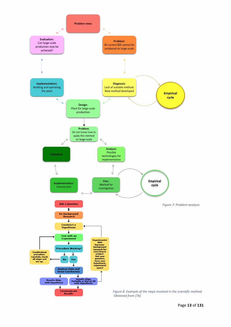
3.1 Problem analysis Based on the above description, it is clear that the main problem, which started the investigation, is the inability to produce BDI on large-scale. By analyzing this problem, it was found that this was due to production method, which is not suitable for large-scale as it makes use of explosive compounds. These are the first phases of the regulative cycle [14], which is used as a problem solving method and is shown in upper cycle in Figure 7. However, since there is no suitable method, the empirical cycle is applied to acquire new knowledge and develop a new method. The next phases in the regulative cycle are Design, in which a design of a plant suitable for large-scale production will be developed; Implementation, in which the plant will be build and operated (tested); Evaluation, during which it is determined whether the problem is solved with solution. All the while this is an iterative process, going back and forth between the phases. For the development of a plant design, technologies must be applied that are suitable for large-scale production. The synthesis route of the newly developed method, however, is only suitable for lab scale. In order to complete the design phase, this problem must be solved, which can be accomplished with jet another regulative cycle, as shown in Figure 7. Now the problem to be solved is the lack of knowledge on how to apply the new method on large-scale. During the analysis phase the synthesis method is examined and the key elements, which ensure that the reaction works, are identified. An investigation is done into technologies, which are suitable for large-scale, that also possess these key elements and thus could possibly perform the reaction. Next, a plan is created on how to proof the concept, and is executed in the implementation phase. In this case it was decided to perform the preliminary study at a toll-manufacturer. During the evaluation phase it was concluded that the reaction itself can be accomplish with the technology. However, there is still a lack of comprehension of the process so that the problem remains unsolved. The regulative cycle is therefore repeated for a second cycle while adopting the knowledge acquired during the first cycle. During the analysis phase theories are developed on the workings of the process and new research questions are formulated, such as:
- What is the operating window? - What factors are important in upscaling? - What factors influence the selectivity and how can we control them?
In the planning phase it was decided to develop a falling film reactor instead renting one to perform the experiments. During this phase the experimental procedures also need to be developed. However, to adequately develop an experimental procedure more general knowledge about the reactor is required, such as how to operate the reactor and what theories are to be applied, which is the focus of this research.
3.2 Methodological Choice Dependent on the orientation of the research a distinction can be made and, associated with this, the methods to be applied. Based on the description of the situation, it can be stated that the intention of the research is to provide (general) knowledge about the falling film reactor designed by the RUG. Therefore, this research is classified as a Knowledge Oriented Research (KOR) and the empirical cycle is than better suited to provide answers. The empirical cycle is still very general and therefore it was chosen to work along the lines of the scientific method. Figure 8 shows an example of steps involved in the scientific method.
Page 13 of 131
Figure 7: Problem analysis
Figure 8: Example of the steps involved in the scientific method. Obtained from [76]
Page 14 of 131
4 Research Proposal The aim of this research is to provide some initial understanding of the falling film reactor. This aim is still very broad and thus, to give focus and guidance to the research, a research goal is developed. One of the basic elements of the reactor is transferring heat, first from the heating elements to the liquid and then from the vapor to the cooling liquid. The flow of the liquid is key on how well the heat is transferred (e.g. formation of dry patches, degree of mixing, which is related to the Reynolds number). Therefore, the research goal of this study will be formulate as:
Characterize the falling film reactor developed by the RUG with respect to its influence on film flow behavior and heat transfer
Based on this research goal, certain knowledge needs to be acquired. To provide direction for this knowledge acquisition research questions will be defined. A literature study will be performed to try and provide answer to these questions, which will be used to determine the direction for specific research. First of all, in order to have a good heat transfer, the heated area needs to be completely covered with liquid. Therefore, the liquid distribution over the perimeter is essential. Furthermore, the film must not breakdown. Secondly, in order to be able to use the falling film reactor, one needs to know what the maximum flowrate is under certain conditions, and what the limiting factors are. Based on this, the following research questions have been proposed:
1. What factors influence the breakdown of the film?
2. What fluid properties influence the liquid distribution?
3. What part of the falling film reactor is the flow limiting section?
4. What determines the heat transfer?
Page 15 of 131
5 Literature Study
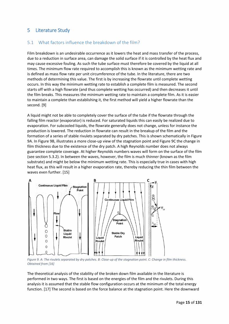
5.1 What factors influence the breakdown of the film? Film breakdown is an undesirable occurrence as it lowers the heat and mass transfer of the process, due to a reduction in surface area, can damage the solid surface if it is controlled by the heat flux and may cause excessive fouling. As such the tube surface must therefore be covered by the liquid at all times. The minimum flow rate required to accomplish this is known as the minimum wetting rate and is defined as mass flow rate per unit circumference of the tube. In the literature, there are two methods of determining this value. The first is by increasing the flowrate until complete wetting occurs. In this way the minimum wetting rate to establish a complete film is measured. The second starts off with a high flowrate (and thus complete wetting has occurred) and then decreases it until the film breaks. This measures the minimum wetting rate to maintain a complete film. As it is easier to maintain a complete than establishing it, the first method will yield a higher flowrate than the second. [9] A liquid might not be able to completely cover the surface of the tube if the flowrate through the falling film reactor (evaporator) is reduced. For saturated liquids this can easily be realized due to evaporation. For subcooled liquids, the flowrate generally does not change, unless for instance the production is lowered. The reduction in flowrate can result in the breakup of the film and the formation of a series of stable rivulets separated by dry patches. This is shown schematically in Figure 9A. In Figure 9B, illustrates a more close-up view of the stagnation point and Figure 9C the change in film thickness due to the existence of the dry patch. A high Reynolds number does not always guarantee complete coverage. At higher Reynolds numbers waves will form on the surface of the film (see section 5.3.2). In between the waves, however, the film is much thinner (known as the film substrate) and might be below the minimum wetting rate. This is especially true in cases with high heat flux, as this will result in a higher evaporation rate, thereby reducing the thin film between the waves even further. [15]
Figure 9. A: The rivulets separated by dry patches. B: Close-up of the stagnation point. C: Change in film thickness. Obtained from [16]
The theoretical analysis of the stability of the broken down film available in the literature is performed in two ways. The first is based on the energies of the film and the rivulets. During this analysis it is assumed that the stable flow configuration occurs at the minimum of the total energy function. [17] The second is based on the force balance at the stagnation point. Here the downward
A B C
Page 16 of 131
stagnation force, which is a result of the conversion of the fluid kinetic energy into static pressure, is equal to the upward surface tension force, which depends on the contact angle of the liquid with the solid surface. In case the downward force is greater, the dry patch is not stable and will wash away. [18] However, if it is stable, the dry patch will heat up. This can lead to violent nucleate boiling once to liquid film is supplied again and thus contamination of the product (condensate). [19] Furthermore, at the boundary of the dry patch the liquid will slow down. In case of a multicomponent mixture such as milk, the volatile components will evaporate more from this part. This will concentrate it and thereby increases the likelihood of fouling. [20] Presented below are two examples of the minimum wetting rate obtained from the force balance and minimum total energy, respectively: [16]
𝛤𝑚𝑖𝑛 = 1.693(1 − 𝑐𝑜𝑠𝜃)3
5(𝜌𝜇𝜎3
𝑔)
1
5 (1)
𝛤𝑚𝑖𝑛 = 1.018(1 − 𝑐𝑜𝑠𝜃)3
5(𝜌𝜇𝜎3
𝑔)
1
5 (2)
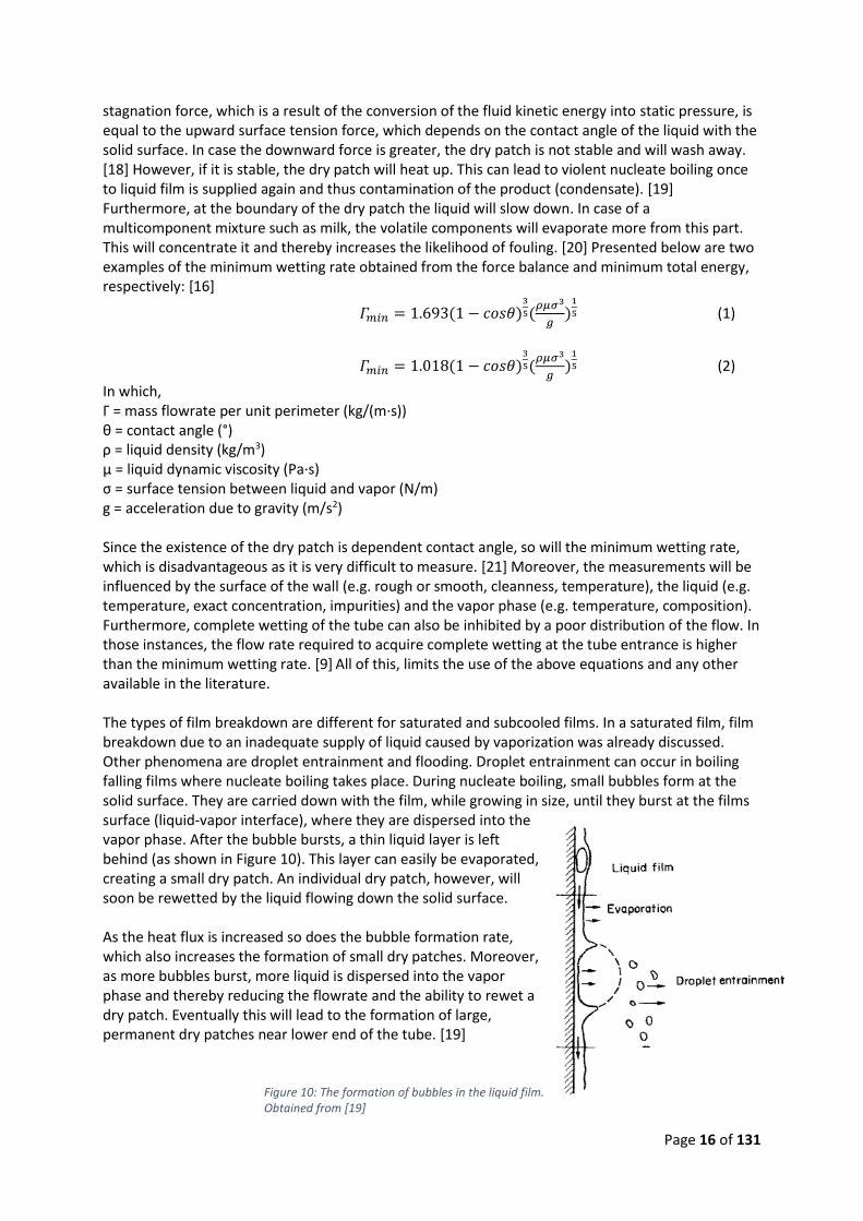
In which, Γ = mass flowrate per unit perimeter (kg/(m·s)) θ = contact angle (°) ρ = liquid density (kg/m3) µ = liquid dynamic viscosity (Pa·s) σ = surface tension between liquid and vapor (N/m) g = acceleration due to gravity (m/s2) Since the existence of the dry patch is dependent contact angle, so will the minimum wetting rate, which is disadvantageous as it is very difficult to measure. [21] Moreover, the measurements will be influenced by the surface of the wall (e.g. rough or smooth, cleanness, temperature), the liquid (e.g. temperature, exact concentration, impurities) and the vapor phase (e.g. temperature, composition). Furthermore, complete wetting of the tube can also be inhibited by a poor distribution of the flow. In those instances, the flow rate required to acquire complete wetting at the tube entrance is higher than the minimum wetting rate. [9] All of this, limits the use of the above equations and any other available in the literature. The types of film breakdown are different for saturated and subcooled films. In a saturated film, film breakdown due to an inadequate supply of liquid caused by vaporization was already discussed. Other phenomena are droplet entrainment and flooding. Droplet entrainment can occur in boiling falling films where nucleate boiling takes place. During nucleate boiling, small bubbles form at the solid surface. They are carried down with the film, while growing in size, until they burst at the films surface (liquid-vapor interface), where they are dispersed into the vapor phase. After the bubble bursts, a thin liquid layer is left behind (as shown in Figure 10). This layer can easily be evaporated, creating a small dry patch. An individual dry patch, however, will soon be rewetted by the liquid flowing down the solid surface. As the heat flux is increased so does the bubble formation rate, which also increases the formation of small dry patches. Moreover, as more bubbles burst, more liquid is dispersed into the vapor phase and thereby reducing the flowrate and the ability to rewet a dry patch. Eventually this will lead to the formation of large, permanent dry patches near lower end of the tube. [19] Figure 10: The formation of bubbles in the liquid film.
Obtained from [19]
Page 17 of 131
Flooding is the other type of film breakdown in saturated films and occurs due to the upward flow of vapor. In cases where the evaporation is condensed externally, the vapor can be removed from the reactor/evaporator countercurrently. Thereby, the shear stresses in the surface of the film are increased, when compared to a stagnant vapor phase. At low vapor velocities these shear stresses are not an issue. However, at higher velocities they can start to slow down the motion of the film. At the flooding point, also known as the onset of flooding, the vapor velocity has reached such a level that the interfacial portion of the film is now carried upwards. At even higher velocities it is even possible to carry the entire liquid film upwards, which is known as climbing film flow. [22] The reduction in the downward liquid flow can lead to the breakdown of the film. This breakdown phenomenon is not considered to be of real importance during this research since the vapor is condensed internally. However, it should be kept in mind when performing the experiments. For subcooled films the most dominant film breakdown method is thermocapillary breakdown. This breakdown is induced by local variations of the surface tension, i.e. Marangoni effects, in the horizontal direction. These variations can be due to temperature. Irregularities in the film thickness cause the thicker regions to have lower temperatures and subsequently higher surface tension. This forces the liquid to start moving from the thin to thick region, which could lead to a liquid deficiency in the thin region and the formation of a dry patch. When higher flowrates or higher inlet temperatures are used, the heat flux necessary to induce film breakdown also increases, as more heat is required to inflict the necessary surface tension gradient. [21] Furthermore, even at high Reynolds numbers it is possible to have thermocapillary breakdown of the film. Now the film will break between the waves, when the film only consists of the substrate. [23]
5.2 What fluid properties influence the liquid distribution? As already mentioned before, the way of distributing the liquid around the tube perimeter is rather unique. To the best of the author’s knowledge, there is no literature available that can provide insight into this particular case with respect to variables involved and to what extent. Therefore, a small qualitative analysis is performed here. Properties that can potentially influence the liquid distribution are:
- Density; determines the magnitude by which the force of gravity acts on the fluid. It is expected that substance with a higher density will be able to form film more easily.
- Degree of wetting; determines how well the adhesion is between the liquid and the wall. This is dependent on the surface energies (tension) between the liquid-gas, liquid-solid and solid-gas. To form a film, the liquid needs to create a large surface area with both the wall as well as with the gas phase. If the wettability is poor, then it can be expected that the formation of a film is difficult, if not impossible.
- Viscosity; the measurement of resistance against flow. It is expected that it will be more difficult to from a uniformly distributed film for substances with higher viscosities.
5.3 What part of the falling film reactor is the flow limiting segment? Figure 1F displays the fluid flows inside the falling film reactor. Based on these flows, different flows were identified that potentially could be the flow limiting section. The first is the liquid level at the bottom of the reaction section. If the outflow from the section is lower than the flowrate, the liquid level between the two walls will start to rise. If the outflow is much lower, the liquid could even overflow into the product section, which would render the process useless and must be avoided. The same could be said for the liquid level in the product section. If the amount that evaporates and condenses is much higher than the amount that can exit the product section, the liquid level will rise.
Page 18 of 131
This could potentially lead to an overflow from the product section back in to the reaction section. For low viscosity fluids this situation seems very unrealistic. However, for more viscous fluids, especially once with a large gradient with respect to temperature, this is not unrealistic. Imagine a situation in which the fluid enters the reactor at near boiling and is thus relativity fluid. Once condensed and cooled down, the viscosity is high and the fluid is relatively immobile. Another limiting flow is the film itself. The thickness of the film must not be larger than the space between the two walls at the bottom of the reaction section (the space where the just mentioned liquid holdup resides). If it is larger, then there will be an overflow into the product section. From Appendix 2 it is clear that the film thickness must be smaller than 4.5 mm. A film can also be formed on cooling tube. The maximum thickness here is 6.5 mm. The inlet is not seen as a limiting factor, since this relies on the pump used. With a big enough pump, any flowrate should possible. The above flows are all concerns with respect to the maximum flowrate. With respect to the minimum flow rate, film breakdown is one of the biggest issues. This has already elaborately been discussed in section 5.1. Furthermore, the distribution of the liquid could also be a limiting factor. It might be possible that the minimum wetting rate cannot be achieved due to the distribution method. This would increase the minimum flowrate and thereby reduces the operating window. In the text below ways to estimate the liquid level and the film thickness will be discussed. The governing equations for the film thickness as well as the liquid level are the same for both the product and the reaction sections and as such will not be individually treated. The main difference is that for the reaction section the liquid flowrate is known, while for the product section this is dependent on the heat transfer, which still needs to be investigated. As already stated there is no literature available that can provide insight into this particular distribution method. If the distribution is an issue will become evident during the experiments.
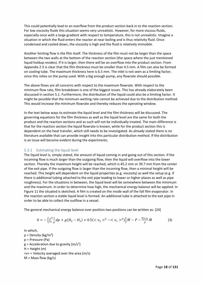
5.3.1 Estimating the liquid level The liquid level is, simply stated, the amount of liquid coming in and going out of this section. If the incoming flow is much larger than the outgoing flow, then the liquid will overflow into the lower section. Thereby the maximum height will be reached, which is 45.2 mm or 39.7 mm from the center of the exit pipe. If the outgoing flow is larger than the incoming flow, then a minimal height will be reached. This height will dependent on the liquid properties (e.g. viscosity) as well the setup (e.g. if there is additional tubing attached to the exit pipe leading to lower or higher places as well as pipe roughness). For the situations in between, the liquid level will be somewhere between the minimum and the maximum. In order to determine how high, the mechanical energy balance will be applied. In Figure 11 the situated is sketched. A film is created on the inside wall of the fall film evaporator. In the reaction section a stable liquid level is formed. An additional tube is attached to the exit pipe in order to be able to collect the outflow in a vessel. The general mechanical energy balance over position two positions can be written as: [24]
In which, ρ = Density (kg/m3) p = Pressure (Pa) g = Acceleration due to gravity (m/s2) H = Height (m) <v> = Velocity averaged over the area (m/s) Ṁ = Mass flow (kg/s)
Page 19 of 131
P = Power supplied to or from system (W) pfric = Pressure drop due to friction, including miscellaneous losses as well as equipment losses (Pa) It should be noted that the term <v2>2-<v1>2 is a simplification and should officially be <v2
3>/<v2> - <v13>/<v1>, however it can be assumed that error is small. [24] pf/ρ is equal to the
amount of mechanical energy converted into heat per unit mass. If the power is negative a pump has to be used. When the density is independent of the pressure, which is the case for the liquids used in this report, equation 3 can be written as:
0 = − {𝑝2
𝜌−
𝑝1
𝜌+ 𝑔(𝐻2 − 𝐻1) + 0.5(< v2 >2 −< v1 >2)} �� − 𝑃 −
𝑝𝑓
𝜌�� (4)
The mechanical energy balance between position 1 and 2 in Figure 11 can be written as:
𝑝1−𝑝2 = −𝜌𝑔𝑧 + 0.5𝜌 < v2 >2+ 𝑝𝑓𝑟𝑖𝑐 (5)
Here it is assumed that the average velocity at position 1 is much smaller than at position 2 and can therefore be neglected. Here the p1 is atmospheric pressure plus hydrostatic pressure of the liquid above its position, which is equal to ρgΔH. ΔH of course being the height for which an estimation is required. p2 is atmospheric pressure and z can be manually measured once the setup is known. The average velocity can be determined when the flow is known.
Figure 11: Sketch of situation over which the mechanical energy balance is applied
The friction can be separated into pressure drop due to the pipeline and to the pipe fittings and valves. For both, the formula’s to be used are dependent on the flow regime (i.e. laminar versus turbulent). The flow regime can be determined by using the dimensionless Reynolds (Re) number, which is defined as: [24]
𝑅𝑒 =𝑖𝑛𝑒𝑟𝑡𝑖𝑎𝑙 𝑓𝑜𝑟𝑐𝑒𝑠
𝑣𝑖𝑠𝑐𝑜𝑢𝑠 𝑓𝑜𝑟𝑐𝑒𝑠=
𝜌v𝐿
𝜇 (6)
In which; ρ = Density (kg/m3) v = Velocity (m/s) μ = Dynamic viscosity (Pa·s) L = Characteristic length (m), which is equal to the hydraulic diameter (Di) of the pipe The hydraulic diameter of a pipe is defined as: [24]
𝐷𝑖 =4𝐴
𝑆 (7)
Page 20 of 131
In which, AC,p = Cross-sectional area of the pipe (m2) S = Circumference of the area of the pipe (m) For a circular pipe the hydraulic diameter is simply the inside diameter of the pipe.
5.3.1.1 Pressure drop due to friction with the pipeline The pressure drop due to viscous effects can be determined with Darcy-Weisbach equation for cylindrical pipes with a uniform diameter: [25]
𝑝𝑓𝑟𝑖𝑐,𝑝 = 𝑓𝜌v2
2
(𝑥2−𝑥1)
𝐷𝑖 (8)
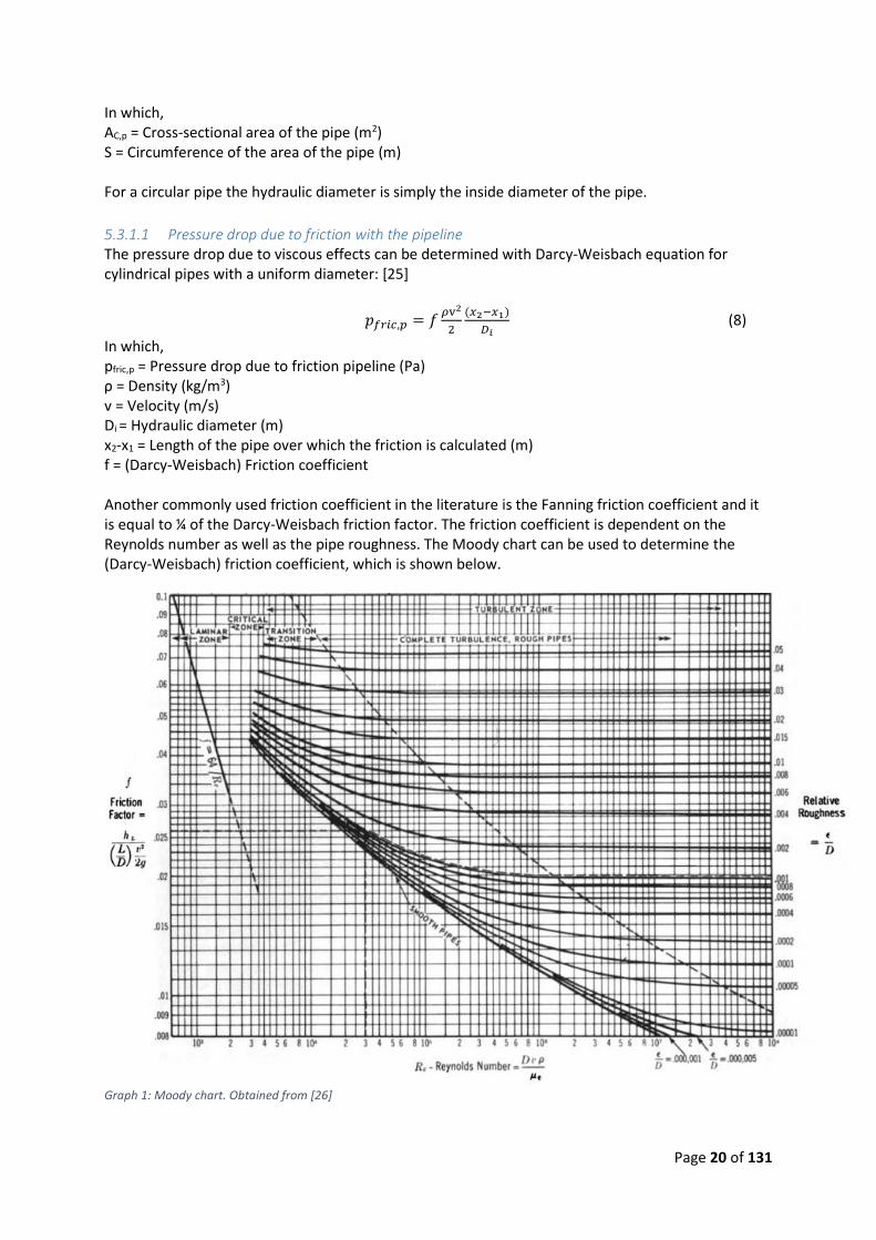
In which, pfric,p = Pressure drop due to friction pipeline (Pa) ρ = Density (kg/m3) v = Velocity (m/s) Di = Hydraulic diameter (m) x2-x1 = Length of the pipe over which the friction is calculated (m) f = (Darcy-Weisbach) Friction coefficient Another commonly used friction coefficient in the literature is the Fanning friction coefficient and it is equal to ¼ of the Darcy-Weisbach friction factor. The friction coefficient is dependent on the Reynolds number as well as the pipe roughness. The Moody chart can be used to determine the (Darcy-Weisbach) friction coefficient, which is shown below.
Graph 1: Moody chart. Obtained from [26]
Page 21 of 131
For smooth pipes expressions have been developed so that figures such as Graph 1 are not required
be consulted for the calculations. In the laminar regime (Re<2100) the Hagen-Poiseuille formula can
be applied, which is defined as: [24, 25]
𝑝𝑓𝑟𝑖𝑐,𝑝 =32𝜇v(𝑥2−𝑥1)
𝐷𝑖2 (9)
In which pfric,p = Pressure drop due to friction pipeline (Pa) μ = Dynamic viscosity (Pa·s) v = Velocity (m/s) Di = Hydraulic diameter (m) x2-x1 = Length of the pipe over which the friction is calculated (m) When the Re is larger than 4000 the flow is always turbulent and different formulas have to be applied. The Blasius formula one of such expressions and provides an accurate estimation for the friction coefficient for 4000 < Re < 105, which is defined as: [24, 25]
𝑓 = 0316𝑅𝑒−0.25 (10) The Hermann equation is applied for higher Re numbers, 2*104 < Re < 2*106: [25]
𝑓 = 0.0054 +0.3964
𝑅𝑒0.3 (11)
For even higher Re numbers the Prandtl and von Kármán equation is applied, 106 < Re: [25, 27]
1
√𝑓= −0.8 + 2 log(𝑅𝑒 √𝑓) (12)
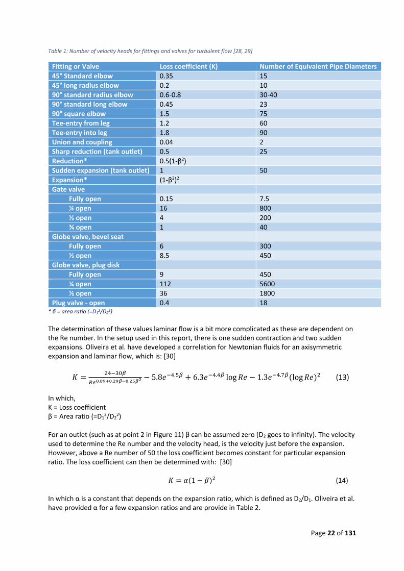
5.3.1.2 Pressure drop due to friction in the pipe fittings and valves The presence of pipe fittings (i.e. bends, contractions, expansions, elbows and tee junctions) as well as valves will influence the flow pattern of the liquid and create turbulence. This turbulence will result in a pressure drop. These miscellaneous pressure losses can be estimated in two ways [28]. The first is by means of the number of velocity heads lost due to obstacle. A velocity head is the amount of kinetic energy contained in a stream, or in other words, it is the potential energy necessary to accelerate the liquid to its velocity. A velocity head is defined as v2/2g meters of fluid, which is equivalent to 0.5ρv2 expressed as a pressure. The number of velocity heads lost due to a valve or fitting is characteristic to a particular valve or fitting and is known as the loss coefficient (K). For turbulent flow these values are independent of the Re number and are thus constant. The loss coefficients for a number of valves and fittings are given in Table 1 for turbulent flow. The second method is by expressing the loss in length of pipe that would otherwise cause the same amount of pressure loss. This is a function of the pipe diameter and therefore the number of equivalent pipe diameter is used. In Table 1 the equivalent pipe diameter for particular valves and fittings are given for turbulent flow. These values then need to be multiplied by the diameter of the pipe used. This value is then added to the actual length of the pipe.
Page 22 of 131
Table 1: Number of velocity heads for fittings and valves for turbulent flow [28, 29]
Fitting or Valve Loss coefficient (K) Number of Equivalent Pipe Diameters
45° Standard elbow 0.35 15
45° long radius elbow 0.2 10
90° standard radius elbow 0.6-0.8 30-40
90° standard long elbow 0.45 23
90° square elbow 1.5 75
Tee-entry from leg 1.2 60
Tee-entry into leg 1.8 90
Union and coupling 0.04 2
Sharp reduction (tank outlet) 0.5 25
Reduction* 0.5(1-β2)
Sudden expansion (tank outlet) 1 50
Expansion* (1-β2)2
Gate valve
Fully open 0.15 7.5
¼ open 16 800
½ open 4 200
¾ open 1 40
Globe valve, bevel seat
Fully open 6 300
½ open 8.5 450
Globe valve, plug disk
Fully open 9 450
¼ open 112 5600
½ open 36 1800
Plug valve - open 0.4 18 * β = area ratio (=D1
2/D22)
The determination of these values laminar flow is a bit more complicated as these are dependent on the Re number. In the setup used in this report, there is one sudden contraction and two sudden expansions. Oliveira et al. have developed a correlation for Newtonian fluids for an axisymmetric expansion and laminar flow, which is: [30]
In which, K = Loss coefficient β = Area ratio (=D1
2/D22)
For an outlet (such as at point 2 in Figure 11) β can be assumed zero (D2 goes to infinity). The velocity used to determine the Re number and the velocity head, is the velocity just before the expansion. However, above a Re number of 50 the loss coefficient becomes constant for particular expansion ratio. The loss coefficient can then be determined with: [30]
𝐾 = 𝛼(1 − 𝛽)2 (14)
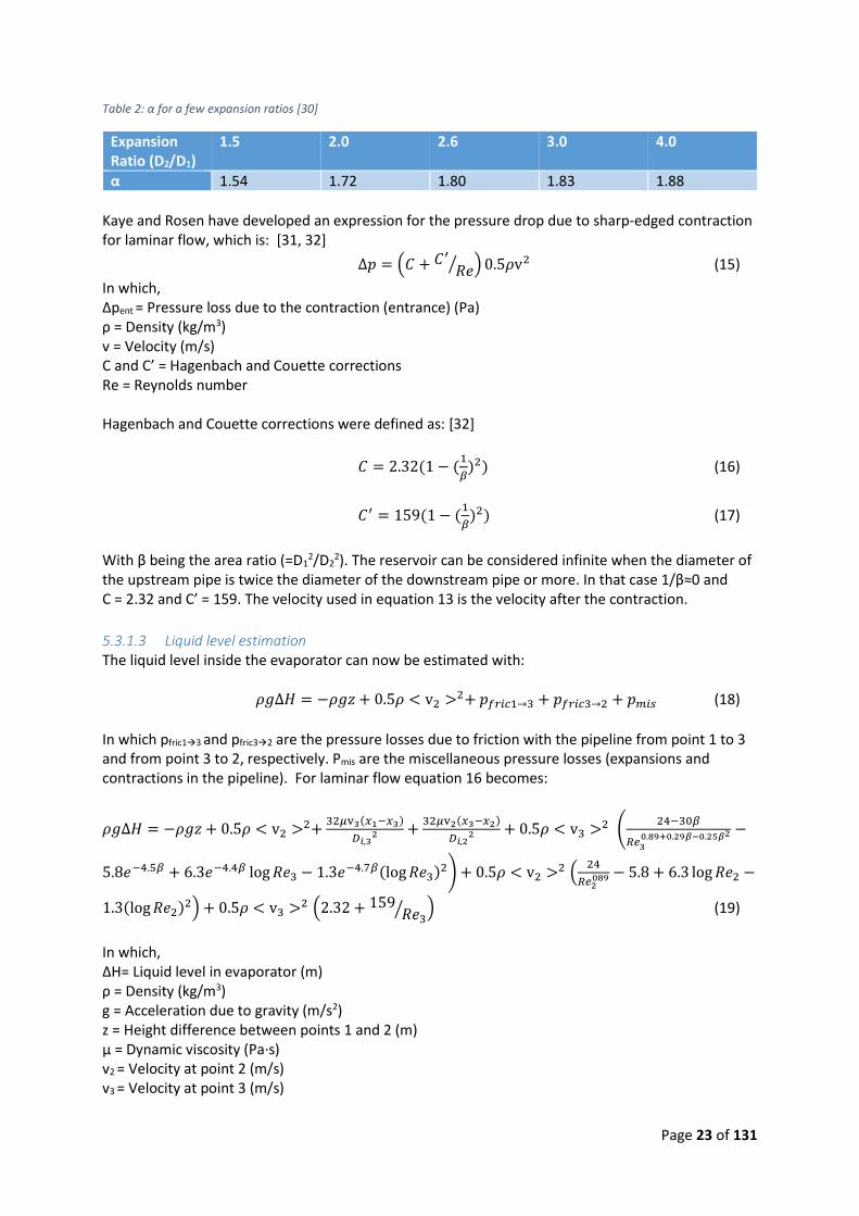
In which α is a constant that depends on the expansion ratio, which is defined as D2/D1. Oliveira et al. have provided α for a few expansion ratios and are provide in Table 2.
Page 23 of 131
Table 2: α for a few expansion ratios [30]
Expansion Ratio (D2/D1)
1.5 2.0 2.6 3.0 4.0
α 1.54 1.72 1.80 1.83 1.88
Kaye and Rosen have developed an expression for the pressure drop due to sharp-edged contraction for laminar flow, which is: [31, 32]
∆𝑝 = (𝐶 + 𝐶′
𝑅𝑒⁄ ) 0.5𝜌v2 (15)
In which, Δpent = Pressure loss due to the contraction (entrance) (Pa) ρ = Density (kg/m3) v = Velocity (m/s) C and C’ = Hagenbach and Couette corrections Re = Reynolds number Hagenbach and Couette corrections were defined as: [32]
𝐶 = 2.32(1 − (1
𝛽)2) (16)
𝐶′ = 159(1 − (1
𝛽)2) (17)
With β being the area ratio (=D1
2/D22). The reservoir can be considered infinite when the diameter of
the upstream pipe is twice the diameter of the downstream pipe or more. In that case 1/β≈0 and C = 2.32 and C’ = 159. The velocity used in equation 13 is the velocity after the contraction.
5.3.1.3 Liquid level estimation The liquid level inside the evaporator can now be estimated with:
In which pfric13 and pfric32 are the pressure losses due to friction with the pipeline from point 1 to 3 and from point 3 to 2, respectively. Pmis are the miscellaneous pressure losses (expansions and contractions in the pipeline). For laminar flow equation 16 becomes:
In which, ΔH= Liquid level in evaporator (m) ρ = Density (kg/m3) g = Acceleration due to gravity (m/s2) z = Height difference between points 1 and 2 (m) μ = Dynamic viscosity (Pa·s) v2 = Velocity at point 2 (m/s) v3 = Velocity at point 3 (m/s)
Page 24 of 131
x1-x3 = Length between points 1 and 3 (m) x3-x2 = Length between points 3 and 2 (m) Di,2 = (hydraulic) Diameter at point 2 (m) Di,3 = (hydraulic) Diameter at point 3 (m) Re2= Reynolds number at point 2 Re3= Reynolds number at point 3 β = Area ratio (=D3
2/D22)
It is assumed that the velocity in the second tube (between points 2 and 3) is the same as at point 2, since the diameter remains unchanged. The same is assumed for the velocity in the exit pipe. This is assumed to be equal to the velocity at point 3. Notice that losses due to bending of the tube attached to the exit pipe are neglected. For turbulent flow equation 16 is a bit more simplistic. For 4000 < Re < 105 it becomes:
The above equations are only valid for hydrodynamically fully developed flow and this must be checked. The entrance length is the length of pipe needed for the flow to acquire a stable velocity profile. This can be determined with the following equations for laminar and turbulent flow, respectively: [33]
𝐿ℎ,𝑝𝑖𝑝𝑒 = 0.05𝑅𝑒𝐷 (22)
𝐿ℎ,𝑝𝑖𝑝𝑒 = 1.359𝐷𝑅𝑒0.25 ≈ 10𝐷 (23)
In which D is the pipe diameter. Again the losses due to bending of the tube attached to the exit pipe are neglected.
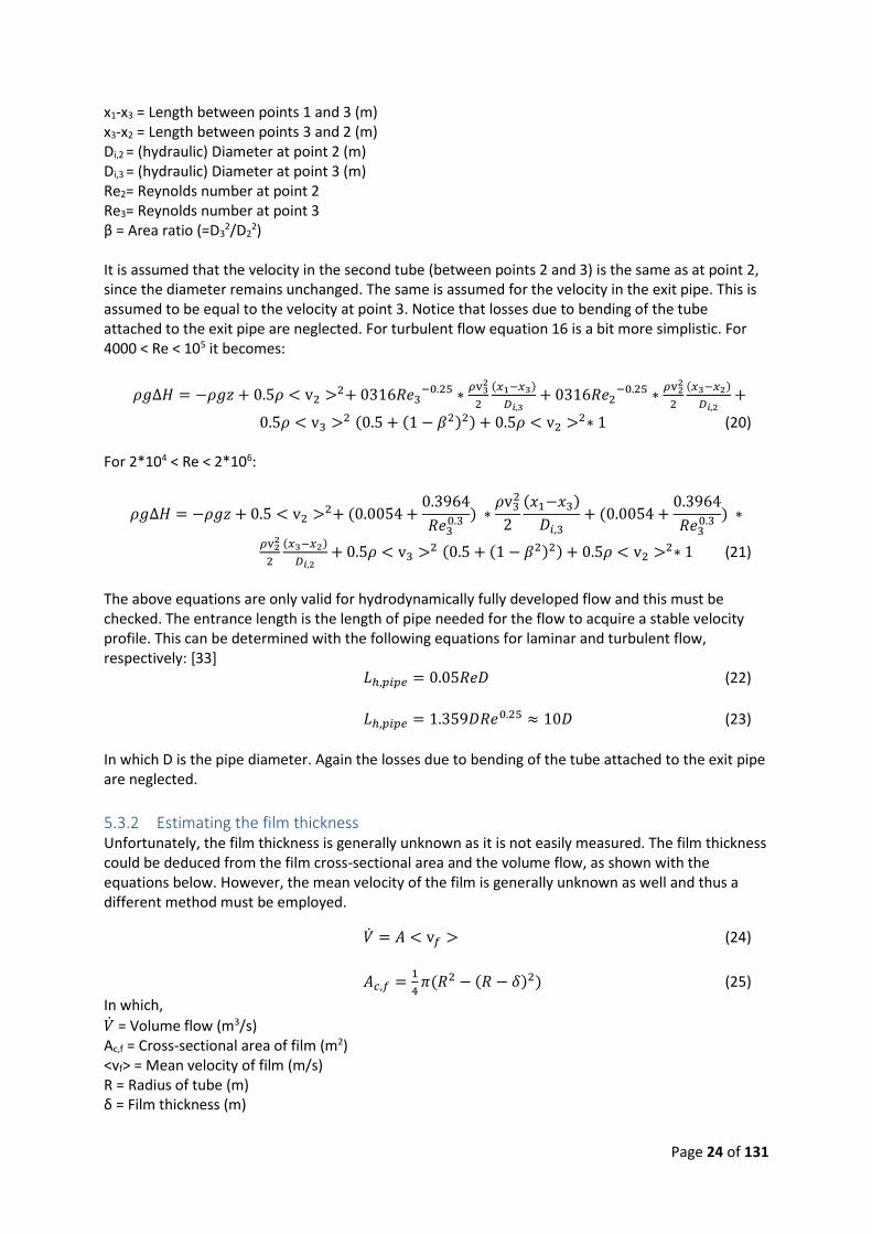
5.3.2 Estimating the film thickness Unfortunately, the film thickness is generally unknown as it is not easily measured. The film thickness could be deduced from the film cross-sectional area and the volume flow, as shown with the equations below. However, the mean velocity of the film is generally unknown as well and thus a different method must be employed.
�� = 𝐴 < v𝑓 > (24)
𝐴𝑐,𝑓 =1
4𝜋(𝑅2 − (𝑅 − 𝛿)2) (25)
In which,
�� = Volume flow (m3/s) Ac,f = Cross-sectional area of film (m2) <vf> = Mean velocity of film (m/s) R = Radius of tube (m) δ = Film thickness (m)
Page 25 of 131
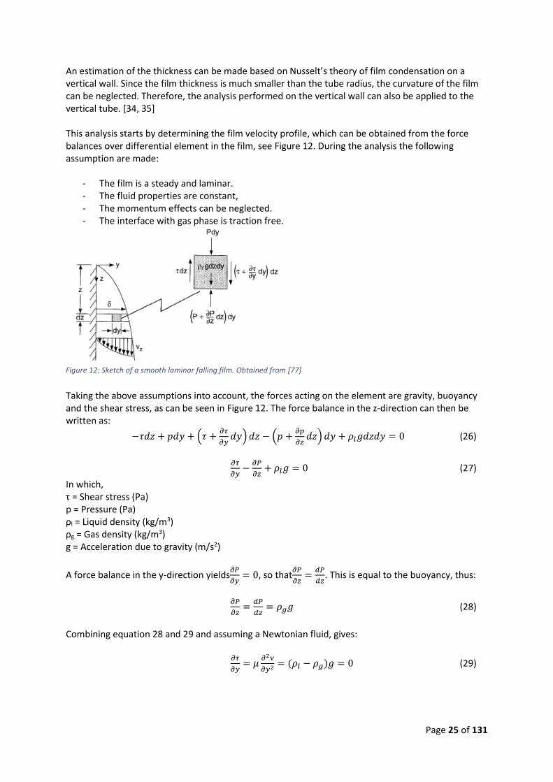
An estimation of the thickness can be made based on Nusselt’s theory of film condensation on a vertical wall. Since the film thickness is much smaller than the tube radius, the curvature of the film can be neglected. Therefore, the analysis performed on the vertical wall can also be applied to the vertical tube. [34, 35] This analysis starts by determining the film velocity profile, which can be obtained from the force balances over differential element in the film, see Figure 12. During the analysis the following assumption are made:
- The film is a steady and laminar. - The fluid properties are constant, - The momentum effects can be neglected. - The interface with gas phase is traction free.
Taking the above assumptions into account, the forces acting on the element are gravity, buoyancy and the shear stress, as can be seen in Figure 12. The force balance in the z-direction can then be written as:
−𝜏𝑑𝑧 + 𝑝𝑑𝑦 + (𝜏 +𝜕𝜏
𝜕𝑦𝑑𝑦) 𝑑𝑧 − (𝑝 +
𝜕𝑝
𝜕𝑧𝑑𝑧) 𝑑𝑦 + 𝜌𝑙𝑔𝑑𝑧𝑑𝑦 = 0 (26)
𝜕𝜏
𝜕𝑦−
𝜕𝑃
𝜕𝑧+ 𝜌𝑙𝑔 = 0 (27)
In which, τ = Shear stress (Pa) p = Pressure (Pa) ρl = Liquid density (kg/m3) ρg = Gas density (kg/m3) g = Acceleration due to gravity (m/s2)
A force balance in the y-direction yields𝜕𝑃
𝜕𝑦= 0, so that
𝜕𝑃
𝜕𝑧=
𝑑𝑃
𝑑𝑧. This is equal to the buoyancy, thus:
𝜕𝑃
𝜕𝑧=
𝑑𝑃
𝑑𝑧= 𝜌𝑔𝑔 (28)
Combining equation 28 and 29 and assuming a Newtonian fluid, gives:
𝜕𝜏
𝜕𝑦= 𝜇
𝜕2v
𝜕𝑦2 = (𝜌𝑙 − 𝜌𝑔)𝑔 = 0 (29)
Figure 12: Sketch of a smooth laminar falling film. Obtained from [77]
Page 26 of 131
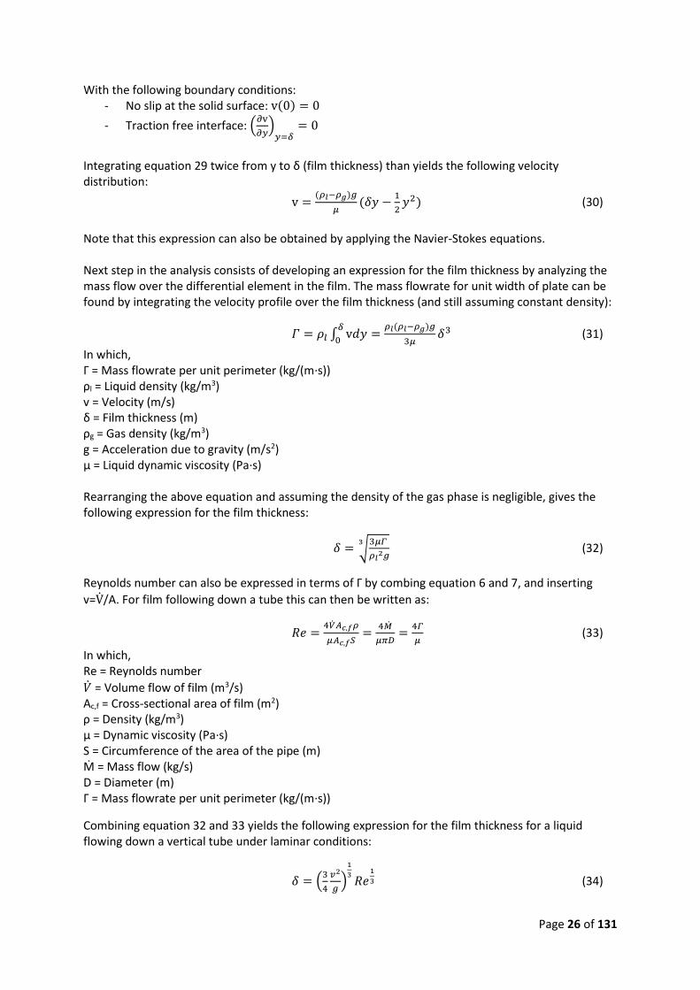
With the following boundary conditions: - No slip at the solid surface: v(0) = 0
- Traction free interface: (𝜕v
𝜕𝑦)
𝑦=𝛿= 0
Integrating equation 29 twice from y to δ (film thickness) than yields the following velocity distribution:
v =(𝜌𝑙−𝜌𝑔)𝑔
𝜇(𝛿𝑦 −
1
2𝑦2) (30)
Note that this expression can also be obtained by applying the Navier-Stokes equations. Next step in the analysis consists of developing an expression for the film thickness by analyzing the mass flow over the differential element in the film. The mass flowrate for unit width of plate can be found by integrating the velocity profile over the film thickness (and still assuming constant density):
𝛤 = 𝜌𝑙 ∫ v𝑑𝑦𝛿
0=
𝜌𝑙(𝜌𝑙−𝜌𝑔)𝑔
3𝜇𝛿3 (31)
In which, Γ = Mass flowrate per unit perimeter (kg/(m·s)) ρl = Liquid density (kg/m3) v = Velocity (m/s) δ = Film thickness (m) ρg = Gas density (kg/m3) g = Acceleration due to gravity (m/s2) μ = Liquid dynamic viscosity (Pa·s) Rearranging the above equation and assuming the density of the gas phase is negligible, gives the following expression for the film thickness:
𝛿 = √3𝜇𝛤
𝜌𝑙2𝑔
3 (32)
Reynolds number can also be expressed in terms of Γ by combing equation 6 and 7, and inserting
v=V/A. For film following down a tube this can then be written as:
𝑅𝑒 =4��𝐴𝑐,𝑓𝜌
𝜇𝐴𝑐,𝑓𝑆=
4��
𝜇𝜋𝐷=
4𝛤
𝜇 (33)
In which, Re = Reynolds number
�� = Volume flow of film (m3/s) Ac,f = Cross-sectional area of film (m2) ρ = Density (kg/m3) μ = Dynamic viscosity (Pa·s) S = Circumference of the area of the pipe (m) Ṁ = Mass flow (kg/s) D = Diameter (m) Γ = Mass flowrate per unit perimeter (kg/(m·s))
Combining equation 32 and 33 yields the following expression for the film thickness for a liquid flowing down a vertical tube under laminar conditions:
𝛿 = (3
4
𝑣2
𝑔)
1
3𝑅𝑒
1
3 (34)
Page 27 of 131
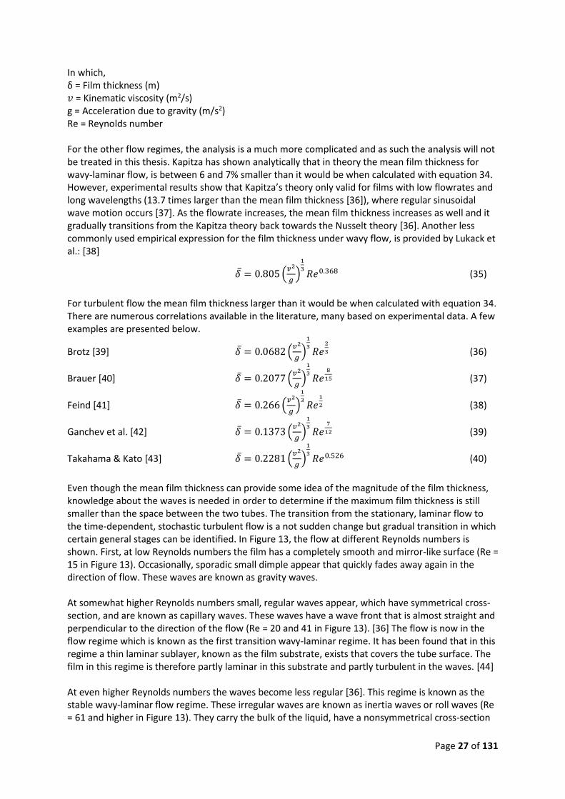
In which, δ = Film thickness (m) 𝑣 = Kinematic viscosity (m2/s) g = Acceleration due to gravity (m/s2) Re = Reynolds number For the other flow regimes, the analysis is a much more complicated and as such the analysis will not be treated in this thesis. Kapitza has shown analytically that in theory the mean film thickness for wavy-laminar flow, is between 6 and 7% smaller than it would be when calculated with equation 34. However, experimental results show that Kapitza’s theory only valid for films with low flowrates and long wavelengths (13.7 times larger than the mean film thickness [36]), where regular sinusoidal wave motion occurs [37]. As the flowrate increases, the mean film thickness increases as well and it gradually transitions from the Kapitza theory back towards the Nusselt theory [36]. Another less commonly used empirical expression for the film thickness under wavy flow, is provided by Lukack et al.: [38]
𝛿 = 0.805 (𝑣2
𝑔)
1
3𝑅𝑒0.368 (35)
For turbulent flow the mean film thickness larger than it would be when calculated with equation 34. There are numerous correlations available in the literature, many based on experimental data. A few examples are presented below.
Brotz [39] 𝛿 = 0.0682 (𝑣2
𝑔)
1
3𝑅𝑒
2
3 (36)
Brauer [40] 𝛿 = 0.2077 (𝑣2
𝑔)
1
3𝑅𝑒
8
15 (37)
Feind [41] 𝛿 = 0.266 (𝑣2
𝑔)
1
3𝑅𝑒
1
2 (38)
Ganchev et al. [42] 𝛿 = 0.1373 (𝑣2
𝑔)
1
3𝑅𝑒
7
12 (39)
Takahama & Kato [43] 𝛿 = 0.2281 (𝑣2
𝑔)
1
3𝑅𝑒0.526 (40)
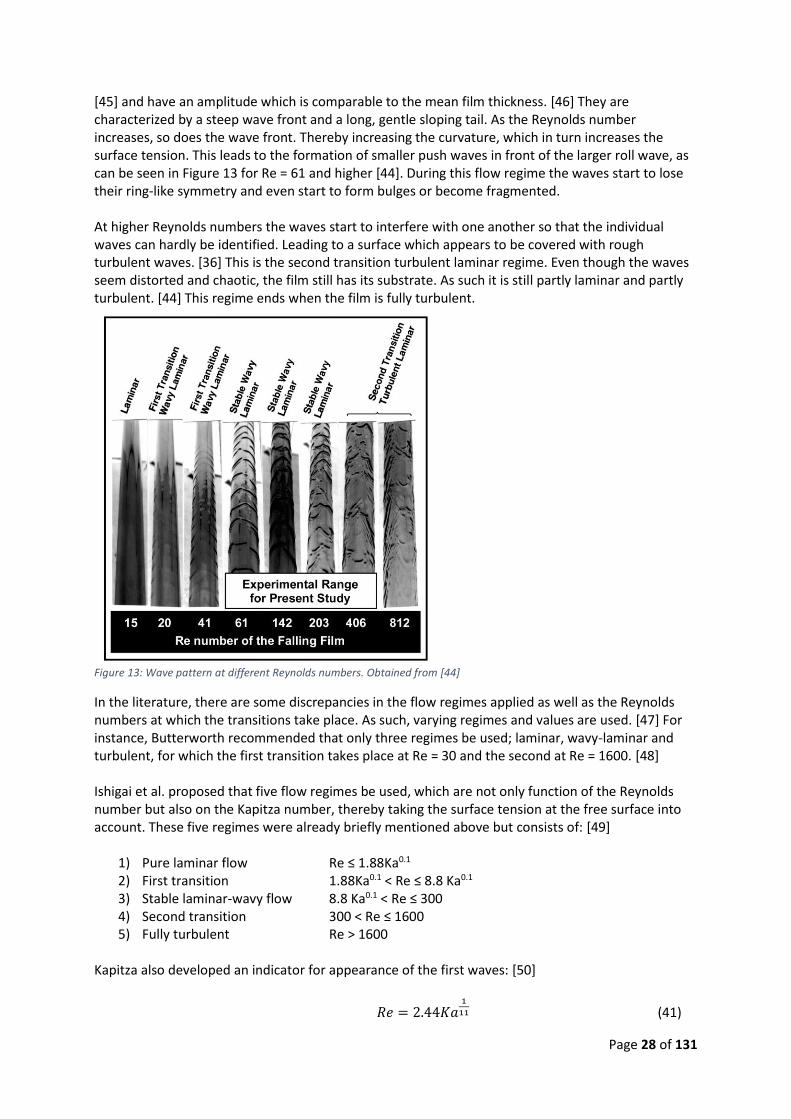
Even though the mean film thickness can provide some idea of the magnitude of the film thickness, knowledge about the waves is needed in order to determine if the maximum film thickness is still smaller than the space between the two tubes. The transition from the stationary, laminar flow to the time-dependent, stochastic turbulent flow is a not sudden change but gradual transition in which certain general stages can be identified. In Figure 13, the flow at different Reynolds numbers is shown. First, at low Reynolds numbers the film has a completely smooth and mirror-like surface (Re = 15 in Figure 13). Occasionally, sporadic small dimple appear that quickly fades away again in the direction of flow. These waves are known as gravity waves. At somewhat higher Reynolds numbers small, regular waves appear, which have symmetrical cross-section, and are known as capillary waves. These waves have a wave front that is almost straight and perpendicular to the direction of the flow (Re = 20 and 41 in Figure 13). [36] The flow is now in the flow regime which is known as the first transition wavy-laminar regime. It has been found that in this regime a thin laminar sublayer, known as the film substrate, exists that covers the tube surface. The film in this regime is therefore partly laminar in this substrate and partly turbulent in the waves. [44] At even higher Reynolds numbers the waves become less regular [36]. This regime is known as the stable wavy-laminar flow regime. These irregular waves are known as inertia waves or roll waves (Re = 61 and higher in Figure 13). They carry the bulk of the liquid, have a nonsymmetrical cross-section
Page 28 of 131
[45] and have an amplitude which is comparable to the mean film thickness. [46] They are characterized by a steep wave front and a long, gentle sloping tail. As the Reynolds number increases, so does the wave front. Thereby increasing the curvature, which in turn increases the surface tension. This leads to the formation of smaller push waves in front of the larger roll wave, as can be seen in Figure 13 for Re = 61 and higher [44]. During this flow regime the waves start to lose their ring-like symmetry and even start to form bulges or become fragmented. At higher Reynolds numbers the waves start to interfere with one another so that the individual waves can hardly be identified. Leading to a surface which appears to be covered with rough turbulent waves. [36] This is the second transition turbulent laminar regime. Even though the waves seem distorted and chaotic, the film still has its substrate. As such it is still partly laminar and partly turbulent. [44] This regime ends when the film is fully turbulent.
Figure 13: Wave pattern at different Reynolds numbers. Obtained from [44]
In the literature, there are some discrepancies in the flow regimes applied as well as the Reynolds numbers at which the transitions take place. As such, varying regimes and values are used. [47] For instance, Butterworth recommended that only three regimes be used; laminar, wavy-laminar and turbulent, for which the first transition takes place at Re = 30 and the second at Re = 1600. [48] Ishigai et al. proposed that five flow regimes be used, which are not only function of the Reynolds number but also on the Kapitza number, thereby taking the surface tension at the free surface into account. These five regimes were already briefly mentioned above but consists of: [49]
1) Pure laminar flow Re ≤ 1.88Ka0.1 2) First transition 1.88Ka0.1 < Re ≤ 8.8 Ka0.1 3) Stable laminar-wavy flow 8.8 Ka0.1 < Re ≤ 300 4) Second transition 300 < Re ≤ 1600 5) Fully turbulent Re > 1600
Kapitza also developed an indicator for appearance of the first waves: [50]
𝑅𝑒 = 2.44𝐾𝑎1
11 (41)
Page 29 of 131
In which the Kapitza (Ka) number is defined as:
𝐾𝑎 =𝜌𝜎3
𝑔𝜇4 (42)
In which, ρ = Density (kg/m3) σ = Surface tension between liquid and vapor (N/m) g = Acceleration due to gravity (m/s2) μ = Dynamic viscosity (Pa·s) It should be noted that in some literature the Reynolds number is defined as Re = Γ/μ, thereby acquiring Reynolds numbers which are only a fourth of the values presented here.
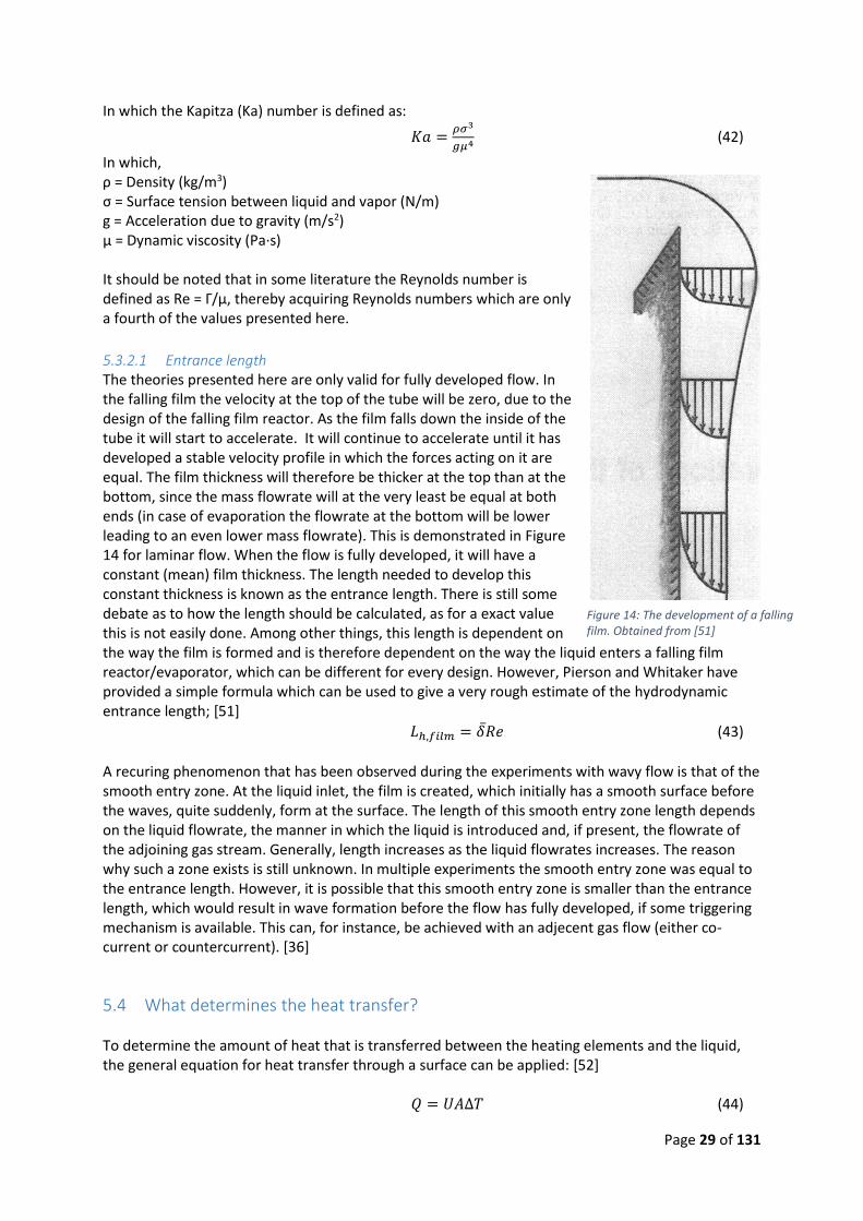
5.3.2.1 Entrance length The theories presented here are only valid for fully developed flow. In the falling film the velocity at the top of the tube will be zero, due to the design of the falling film reactor. As the film falls down the inside of the tube it will start to accelerate. It will continue to accelerate until it has developed a stable velocity profile in which the forces acting on it are equal. The film thickness will therefore be thicker at the top than at the bottom, since the mass flowrate will at the very least be equal at both ends (in case of evaporation the flowrate at the bottom will be lower leading to an even lower mass flowrate). This is demonstrated in Figure 14 for laminar flow. When the flow is fully developed, it will have a constant (mean) film thickness. The length needed to develop this constant thickness is known as the entrance length. There is still some debate as to how the length should be calculated, as for a exact value this is not easily done. Among other things, this length is dependent on the way the film is formed and is therefore dependent on the way the liquid enters a falling film reactor/evaporator, which can be different for every design. However, Pierson and Whitaker have provided a simple formula which can be used to give a very rough estimate of the hydrodynamic entrance length; [51]
𝐿ℎ,𝑓𝑖𝑙𝑚 = 𝛿𝑅𝑒 (43)
A recuring phenomenon that has been observed during the experiments with wavy flow is that of the smooth entry zone. At the liquid inlet, the film is created, which initially has a smooth surface before the waves, quite suddenly, form at the surface. The length of this smooth entry zone length depends on the liquid flowrate, the manner in which the liquid is introduced and, if present, the flowrate of the adjoining gas stream. Generally, length increases as the liquid flowrates increases. The reason why such a zone exists is still unknown. In multiple experiments the smooth entry zone was equal to the entrance length. However, it is possible that this smooth entry zone is smaller than the entrance length, which would result in wave formation before the flow has fully developed, if some triggering mechanism is available. This can, for instance, be achieved with an adjecent gas flow (either co-current or countercurrent). [36]
5.4 What determines the heat transfer? To determine the amount of heat that is transferred between the heating elements and the liquid, the general equation for heat transfer through a surface can be applied: [52]
𝑄 = 𝑈𝐴∆𝑇 (44)
Figure 14: The development of a falling film. Obtained from [51]
Page 30 of 131
In which: Q = Heat transferred through the surface per unit time (W) U = Overall heat transfer coefficient (W/(m2·°C)) A = Heat transfer area (m2) ΔT = Temperature difference between the wall and the bulk of the liquid film (°C) Heat transferred through the surface per unit time in case of evaporative heating and sensible heating can be determined with the following equations, respectively:
𝑄 = ��𝑣𝑎𝑝∆𝐻𝑣𝑎𝑝 (45)
𝑄 = 𝑐𝑝��(𝑇𝑜𝑢𝑡 − 𝑇𝑖𝑛) (46)
In which,
Mvap = Mass flow rate of evaporation (kg/s) ΔHvap = Enthalpy of vaporization (J/kg) cp = Specific heat capacity (J/(kg·K)) Tout = Outgoing temperature of the film (°C) Tin = Incoming temperature of the film (°C) The overall heat transfer coefficient consists of all the resistances posed by the film, tube wall, heating elements and fouling. In its broadest sense, the overall heat transfer coefficient is defined as: [52]
1
𝑈=
1
ℎ+ 𝑅𝐹,𝑓 +
𝑒
𝜆
𝐴
𝐴𝑚+ (
1
ℎ𝑜+ 𝑅𝐹,𝑜)
𝐴
𝐴𝑜 (47)
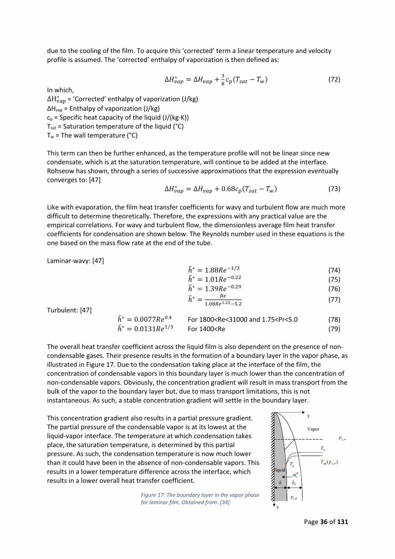
In which, h = Film heat transfer coefficient (W/(m2·°C)) RF,f = Fouling resistance of the film (m2·°C/W) e = Tube wall thickness (m) λ = Thermal conductivity (W/(m·°C)) A = Heat transfer area, also used on eq. 44 (m2) Ao = Heat transfer area on the outside of the tube (heating elements) (m2) Am = Logarithmic mean of A and Ao (m2) ho = Heat transfer coefficient on the outside of the tube (heating elements) (W/(m2·°C)) RF,o = Fouling resistance on the outside of the tube (heating elements) (m2·°C/W) Most of the resistance is imposed by the liquid film. The falling film reactor will be cleaned thoroughly and as such there is no fouling resistance on the film side. Moreover, there is no fouling in the outside, as there is no flow. The reactor is made of stainless steel which has a high thermal conductivity, as such the resistance posed by the tube wall is trivial. The heat transfer coefficient of heating elements will be assumed to be negligible. In order to be able to determine the amount of heat transferred, the film heat transfer coefficient is required. Unfortunately, due to the reactor rather unique design, in which condensation occurs internally without a rotor, there is no literature available on the heat transfer coefficient in such a system. Therefore, the film heat transfer coefficient for evaporation (and heating of subcooled liquids) and condensation will be treated separately. Even though those heat transfer coefficients were obtained in a different process, they might still be able to provide guidance.
5.4.1 Evaporation For evaporation of the liquid film two boiling regimes are identified: nucleate boiling and non-nucleate boiling. Nucleate boiling takes place at higher heat fluxes or temperature differences, while non-nucleate boiling at lower heat fluxes or temperature differences. Although, a distinctive transition has not yet been identified. [53] As already briefly discussed in section 5.1, during nucleate
Page 31 of 131
boiling bubbles are formed at nucleation sites on the solid surface. There are carried down with the film until they burst at the liquid-vapor interface. As the heat flux increases, so does the bubble formation rate, which enhances the heat transfer. This reduces the effect of the film flow on the heat transfer coefficient. Eventually the nucleate boiling heat transfer coefficient is solely dependent on the heat flux (or temperature difference), as shown empirically by Fujita and Ueda: [19]
ℎ = 1.24𝑞0.741 (48) In which q is the heat flux (W/m2) and h the film heat transfer coefficient for nucleate boiling (W/(m2°C)). The film heat transfer coefficients for nucleate boiling are generally higher than for non-nucleate boiling. [19] During non-nucleate boiling, evaporation only takes place at the interface between the liquid and vapor phase. Therefore, the film heat transfer coefficient is dependent on how well the heat is transferred across the film. As such, the film heat transfer coefficient is a function of the flow pattern but not the flux or the temperature difference. [54] How the flow pattern influences the heat transfer coefficient is determined by the flow regime, as heat transfer mechanism differs per regime. The different regimes and the transitions between them were already discussed in section 5.3.2. As such, only the difference in heat transfer mechanisms will be briefly discussed here. In pure laminar flow, the heat is transferred only by conduction and thus the local heat transfer coefficient is defined as the thermal conductivity divided by the local film thickness. Therefore, with an increase in film thickness, the resistance of the film will be higher and thus the heat transfer coefficient will be lower. The Nusselt film thickness (see equation 34) can be applied to determine the local heat transfer coefficient for laminar: [55]
ℎ𝑥 =𝜆
𝛿= 𝜆 [
4𝑔
3𝑣2𝑅𝑒]
1/3 (49)
In which, hx = Local film heat transfer coefficient (W/(m2·°C)) λ = Thermal conductivity (W/(m·°C)) δ = Film thickness (m) g = acceleration due to gravity (m/s2) Re = Reynolds number 𝑣 = kinematic viscosity (m2/s) In the literature the dimensionless heat transfer coefficient is generally applied, which is defined as:
ℎ∗ =ℎ
𝜆(
𝑣2
𝑔)
1/3
(50)
This equal to the films Nusselt number (Nu=h·L/λ), for which 𝑣2
𝑔⁄1/3
is used as length instead of the
film thickness, as this depends on the Reynolds number. [56] As such, the dimensionless local film heat transfer coefficient can be rewritten as:
ℎ𝑥∗ = (
4
3)
1
3𝑅𝑒−
1
3 = 1.1𝑅𝑒−1
3 (51)
The average film heat transfer coefficient can be determined with the following expression. In reference [55] the complete derivation of this expression can be found.
Page 32 of 131
ℎ∗ = −𝑅𝑒𝑖𝑛−𝑅𝑒𝑜𝑢𝑡
∫1
ℎ𝑥𝑑𝑅𝑒
𝑅𝑒𝑜𝑢𝑡𝑅𝑒𝑖𝑛
(52)
Here Rein is the Reynolds number at the inlet and Reout at the outlet. The expression is valid for all flow regimes. By coming equation 49 and 50, an expression for the average film heat transfer coefficient for laminar flow is found;
ℎ∗ = 1.1𝑅𝑒𝑖𝑛−𝑅𝑒𝑜𝑢𝑡
𝑅𝑒𝑖𝑛4/3
−𝑅𝑒𝑜𝑢𝑡4/3 (53)
The above expression is valid for both evaporation and sensible heating, as well as heating with a constant wall temperature and a constant heat flux. [56] However, if the change in Reynolds number is small the average film heat transfer coefficient will be equal to the local film heat transfer coefficient. For sensible heating an empirical correlation for the local heat transfer coefficient has been developed by Wilke; [57, 58, 59]
ℎ𝑥∗ = 2.07𝑅𝑒−
1
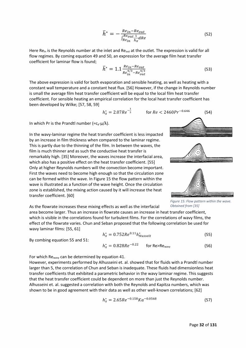
3 for 𝑅𝑒 < 2460𝑃𝑟−0.646 (54) In which Pr is the Prandtl number (=cp·µ/λ). In the wavy-laminar regime the heat transfer coefficient is less impacted by an increase in film thickness when compared to the laminar regime. This is partly due to the thinning of the film. In between the waves, the film is much thinner and as such the conductive heat transfer is remarkably high. [35] Moreover, the waves increase the interfacial area, which also has a positive effect on the heat transfer coefficient. [55] Only at higher Reynolds numbers will the convection become important. First the waves need to become high enough so that the circulation zone can be formed within the wave. In Figure 15 the flow pattern within the wave is illustrated as a function of the wave height. Once the circulation zone is established, the mixing action caused by it will increase the heat transfer coefficient. [60] As the flowrate increases these mixing effects as well as the interfacial area become larger. Thus an increase in flowrate causes an increase in heat transfer coefficient, which is visible in the correlations found for turbulent films. For the correlations of wavy films, the effect of the flowrate varies. Chun and Seban proposed that the following correlation be used for wavy laminar films: [55, 61]
ℎ𝑥∗ = 0.752𝑅𝑒0.11ℎ𝑁𝑢𝑠𝑠𝑒𝑙𝑡
∗ (55) By combing equation 55 and 51:
ℎ𝑥∗ = 0.828𝑅𝑒−0.22 for Re>Rewavy (56)
For which Rewavy can be determined by equation 41. However, experiments performed by Alhusseini et. al. showed that for fluids with a Prandtl number larger than 5, the correlation of Chun and Seban is inadequate. These fluids had dimensionless heat transfer coefficients that exhibited a parametric behavior in the wavy laminar regime. This suggests that the heat transfer coefficient could be dependent on more than just the Reynolds number. Alhusseini et. al. suggested a correlation with both the Reynolds and Kapitza numbers, which was shown to be in good agreement with their data as well as other well-known correlations; [62]
ℎ𝑥∗ = 2.65𝑅𝑒−0.158𝐾𝑎−0.0568 (57)
Figure 15: Flow pattern within the wave. Obtained from [35]
Page 33 of 131
For sensible heating and wavy flow the empirical correlation of Wilke is generally applied: [57, 58, 59]
ℎ𝑥∗ = 0.0323𝑅𝑒1/5𝑃𝑟0.344 for 2460𝑃𝑟−0.646 < 𝑅𝑒 < 1600 (58)
The most commonly applied correlation for evaporative turbulent flow, is provided by Chun Seban: [55, 54, 35, 45, 61]
ℎ𝑥∗ = 3.8 ∙ 10−3𝑅𝑒0.4𝑃𝑟0.65 for 320<Re<21000 and 1.77<Pr<5.7 (59)
Shmerler and Mudawar found a slightly different correlation based on their data: [63]
ℎ𝑥∗ = 3.8 ∙ 10−3𝑅𝑒0.35𝑃𝑟0.95 for 4990<Re<37620 and 1.75<Pr<5.42 (60)
For multicomponent mixtures the following expression is suggested, as the previously discussed expressions might otherwise results in an overestimating of the heat transfer coefficient; [35]
ℎ𝑥∗ = 0.003𝑅𝑒0.44𝑃𝑟0.4 (61)
The empirical correlations of Wilke are generally suggested for sensible heating: [57, 58, 59]
ℎ𝑥∗ = 0.00102𝑅𝑒2/3𝑃𝑟0.344 for 1600<Re<3200 (62)
ℎ𝑥∗ = 0.00871𝑅𝑒2/5𝑃𝑟0.344 for 3200<Re and 5.4<Pr<210 (63)
However, other empirical correlations are also available: [57]
ℎ𝑥∗ = 0.0106𝑅𝑒0.3𝑃𝑟0.63 for 2500<Re<39500 and 2.55<Pr<6.87 (64)
ℎ𝑥∗ = 6.832 ∙ 10−4(𝑅𝑒0.4829𝑃𝑟0.93717 −
21817.84
𝑅𝑒) for 4000<Re<20000 and 1.8<Pr<4.4 (65)
ℎ𝑥∗ = 0.00462𝑅𝑒0.429𝑃𝑟1/3 for 800<Re<7000 and 2.55<Pr<7.2 (66)
Al these correlations can be used in combination with equation 50 to determine the average heat transfer coefficient.
5.4.1.1 Entrance length The above expressions are only valid for thermally developed flow. The flow starts off by developing a thermal boundary layer, which increases in width as the liquid flows down the heated wall. The flow is thermally developed once the thermal boundary layer stresses across the entire film thickness. What this actually entails, and thus how long the thermal entrance length is, depends on specific situation (e.g. sensible vs evaporative heating, constant temperature vs constant heat flux, type of flow regime). In all cases this starts with the development of the thermal boundary layer at the wall (e.g. a rise in temperature of liquid at/near the wall). Once the wall boundary layer been established, the energy input at the wall will raise the bulk temperature. [63] For sensible heating the flow is now fully developed. In cases of constant heat flux, the wall temperature will increase as the bulk temperature increases, resulting in a constant temperature differential between the wall and the surface (assuming an adiabatic interface and that the heat transfer coefficient does not change too drastically). In cases of constant wall temperature, the temperature differential will decrease along the tube length, resulting in a lowering of the heat flux (again assuming the heat transfer coefficient does not change significantly). The flow regime influences how quickly (in terms of tube length) the thermal boundary layer is developed.
Page 34 of 131
In cases of evaporative heating the development of the thermal boundary layer has an additional stage. When the effects of the heat transfer reach the film interface, the liquid will evaporate. The evaporative process, however, causes an energy loss, which results in another temperature gradient within the film. This delays the formation of fully-developed flow and thereby increases the entrance length. Due to the constant temperature of the liquid, the cases of constant heat flux and constant wall temperature are identical (e.g. with a constant heat flux the wall temperature is constant and vice versa). Figure 16 illustrates the development of the thermal boundary layer in a turbulent flow when a constant heat flux is applied for sensible and evaporative heating. This clearly demonstrates the differences in the temperature profile development for the two specific situations.
Figure 16: The differences in the thermal development between sensible (left) and evaporative heating (right), for a hydrodynamically fully developed turbulent flow heated with a constant heat flux. Obtained from [57].
The result of this thermal development region is that the heat transfer coefficient is higher in the entrance length when compared to the heat transfer coefficients in thermally developed flow. This due to the temperature of the liquid in the thermal boundary layer which is lower in this region when compared to the situation of fully developed flow, while the heat flux remains equal. As the flow develops thermally, the temperature in the thermal boundary layer increases and as a result the heat transfer coefficient decreases. This has been shown by Shmerler and Mudawwar experimentally for both sensible and evaporative heating for a turbulent flow with a constant heat flux. [63, 64] With respect to determine the actual length of the thermal entrance region, only a few publications are available in the literature. The first were made by Nakoryakov and Grigorjeva in 1980, who proposed the following expression for the thermal entry length under smooth laminar conditions with sensible heating: [65]
𝐿𝑡,𝑓 = 0.06𝑅𝑒𝑖𝑛4/3
𝑃𝑟𝑖𝑛 (𝑣2
𝑔)
1/3
(67)
In which the Reynolds and Prandtl number are calculated based on the inflow conditions. Mitrović had performed in similar experiment in 1988 and came to a comparable correlation, only differing in the constant applied (0.0974 instead of 0.06). [66] However, it is unrealistic to use the inlet conditions for the calculation of the Prandtl number. As the temperature increases along the tube length, the Prandtl number decreases, thereby decreasing the entrance length. In a more recent study this aspect has been incorporated into the correlation as well as effects of surface tension and waves. Lel and Kneer have therefore suggested the following correlations for wavy laminar flow: [15]
𝐿𝑡,𝑓𝑖𝑙𝑚 = 0.8367𝑅𝑒𝑖𝑛0.718𝑃𝑟𝑖𝑛𝐾𝑎𝑖𝑛
0.0606 (𝑃𝑟𝑖𝑛
𝑃𝑟𝑊)
−0.29(
𝑣2
𝑔)
1/3
for Re<8 (68)
Page 35 of 131
𝐿𝑡,𝑓 = 0.022𝑅𝑒𝑖𝑛1.36𝑃𝑟𝑖𝑛𝐾𝑎𝑖𝑛
0.0606 (𝑃𝑟𝑖𝑛
𝑃𝑟𝑊)
−0.29(
𝑣2
𝑔)
1/3
for Re>8 (69)
In which PrW is the Prandtl number based on the temperature at the wall. The above discussion is only applicable to hydrodynamically developed flow. However, for hydrodynamically and thermally developing flow should still be rather similar. Only difference now is that it might take longer for the thermal boundary layer to reach the surface due to an increase in film thickness (see section 5.3.2.1). But this is only an issue of the flow takes longer to develop hydrodynamically than thermally.
5.4.2 Condensation Condensation can occur dropwise, in which case droplets will be formed on the cooled surface, or filmwise, in which case a thin film will be formed. Which type of condensation occurs, depends on whether the surface is wettable with the condensate or not. If the surface is wettable filmwise condensation occurs, if it is non-wettable dropwise occurs. [34] In this specific case it is most likely that a filmwise condensation occurs instead of dropwise, since the material of the heated surface is exactly the same as the cooled surface. In order to have a good falling film, it is highly likely (although not yet proven) that the wettability needs to be good. Although the wettability of the cooled and heated surfaces is not exactly the same, due to temperature differences, it is still highly probable that the cooled surface is wettable. As such, only the filmwise condensation will be briefly discussed. As for filmwise condensation, all the previous discussions with respect to heat transfer (equations 42-45), wave patterns, flow regime, flow regime transitions and heat mechanisms are all applicable to filmwise condensation as well. Therefore, only the heat transfer coefficient will be given. For laminar flow the classical Nusselt analysis can be used to determine theoretically the film heat transfer coefficient. The complete analysis can be found in [34]. One of its main assumptions is that there is no subcooling at the liquid-vapor interface. It is shown that the average film heat transfer coefficient over the entire length of the film is then equal to:
ℎ∗ = 1.47𝑅𝑒𝑜𝑢𝑡−1/3
(70)
Reout is the Reynolds number at the end of the tube and is related to the film thickness with equation 34. The film thickness can then be determined with the following formula:
𝛿 = [4𝜆µ𝐿𝑓𝛥𝑇
𝜌(𝜌−𝜌𝑣)𝑔𝛥𝐻𝑣𝑎𝑝]
1/4
(71)
In which, λ = Thermal conductivity of liquid (W/(m·°C)) δ = Film thickness (m) g = Acceleration due to gravity (m/s2) µ = Dynamic viscosity of liquid (Pa·s) ΔT = Temperature difference between the wall and saturation temperature of liquid (°C) Lf= Film length (m) ρ = Density of liquid (kg/m3) ρv = Density of vapor (kg/m3) ΔHvap = Enthalpy of vaporization (J/kg) The effects of subcooling can be taken into account in the analysis by applying the ‘corrected’ enthalpy of vaporization, which now not only includes the heat released due condensation but also
Page 36 of 131
due to the cooling of the film. To acquire this ‘corrected’ term a linear temperature and velocity profile is assumed. The ‘corrected’ enthalpy of vaporization is then defined as:
∆𝐻𝑣𝑎𝑝∗ = ∆𝐻𝑣𝑎𝑝 +
3
8𝑐𝑝(𝑇𝑠𝑎𝑡 − 𝑇𝑤) (72)
In which, ∆Hvap
∗ = ‘Corrected’ enthalpy of vaporization (J/kg)
ΔHvap = Enthalpy of vaporization (J/kg) cp = Specific heat capacity of the liquid (J/(kg·K)) Tsat = Saturation temperature of the liquid (°C) Tw = The wall temperature (°C) This term can then be further enhanced, as the temperature profile will not be linear since new condensate, which is at the saturation temperature, will continue to be added at the interface. Rohseow has shown, through a series of successive approximations that the expression eventually converges to: [47]
∆𝐻𝑣𝑎𝑝∗ = ∆𝐻𝑣𝑎𝑝 + 0.68𝑐𝑝(𝑇𝑠𝑎𝑡 − 𝑇𝑤) (73)
Like with evaporation, the film heat transfer coefficients for wavy and turbulent flow are much more difficult to determine theoretically. Therefore, the expressions with any practical value are the empirical correlations. For wavy and turbulent flow, the dimensionless average film heat transfer coefficients for condensation are shown below. The Reynolds number used in these equations is the one based on the mass flow rate at the end of the tube. Laminar-wavy: [47]
ℎ∗ = 1.88𝑅𝑒−1/3 (74)
ℎ∗ = 1.01𝑅𝑒−0.22 (75)
ℎ∗ = 1.39𝑅𝑒−0.29 (76)
ℎ∗ =𝑅𝑒
1.08𝑅𝑒1.22−5.2 (77)
Turbulent: [47]
ℎ∗ = 0.0077𝑅𝑒0.4 For 1800<Re<31000 and 1.75<Pr<5.0 (78)
ℎ∗ = 0.0131𝑅𝑒1/3 For 1400<Re (79)
The overall heat transfer coefficient across the liquid film is also dependent on the presence of non-condensable gases. Their presence results in the formation of a boundary layer in the vapor phase, as illustrated in Figure 17. Due to the condensation taking place at the interface of the film, the concentration of condensable vapors in this boundary layer is much lower than the concentration of non-condensable vapors. Obviously, the concentration gradient will result in mass transport from the bulk of the vapor to the boundary layer but, due to mass transport limitations, this is not instantaneous. As such, a stable concentration gradient will settle in the boundary layer. This concentration gradient also results in a partial pressure gradient. The partial pressure of the condensable vapor is at its lowest at the liquid-vapor interface. The temperature at which condensation takes place, the saturation temperature, is determined by this partial pressure. As such, the condensation temperature is now much lower than it could have been in the absence of non-condensable vapors. This results in a lower temperature difference across the interface, which results in a lower overall heat transfer coefficient.
Figure 17: The boundary layer in the vapor phase for laminar film. Obtained from: [34]
Page 37 of 131
5.5 Specific Research Topics The one of the most important aspects that needs clarification is the liquid distribution and its influence on the formation of the film. In order to be able to do any other experiments, a liquid needs to be able to form a film. As such, the minimum wetting rates will be investigated as a function of different material properties. In the literature the transition between the different flow regimes is somewhat unclear. It is, therefore, interesting to see when the flow start to transition in this falling film reactor. Since the miscellaneous pressure losses are generally smaller than pressure losses due friction with pipeline, it might be possible to simply equations 19 - 21. If not, the miscellaneous pressure losses might be higher than expected from the literature. From inspection of the reactor, it was observed that the inlet of the horizontal tube is not smooth but that there is some metal facing inwards, which formed during manufacturing of the reactor (see Figure 18). This might increase the actual miscellaneous pressure losses resulting in a higher liquid level when compared to values calculated with formulas 19 - 21. Therefore, investigation into the effects of this will be done. Moreover, applicability of the formulas of the film thickness will also be tested. Another important aspect is the determination of the limitation of the process. Where is it and what is it related to (heating, cooling or somewhere else)? And when does film breakdown become an issue? The limitations will be analyzed based on the difference between the heat transfer coefficient determined with measured data and calculated based on the literature for both sensible and evaporative heating. Moreover, film breakdown will be investigated as a function of different inlet temperatures in combination with different heating temperatures.
Figure 18: Inlet of the horizontal tube
Page 38 of 131
6 Experimental Procedures In Appendix 4 a full description is given of each experiment including the experimental setup, the exact procedure followed during the experiments, process flow diagrams, as well as the HAZOP. Since this is rather elaborate and tedious, the individual experiments will only briefly be discussed here as well as a general setup of the experiments. For all observational experiments as well as for most (unexpected) observations made during the other experiments, videos are made so that the specific cases can be better compared with one another. Moreover, it is hoped that this also increases the transferability of knowledge. To increase the observability of the liquid, colored dye is sometimes added to the liquid, which is why the color is sometimes red or green. The liquid distribution and its influence on the formation of the film will be investigated for several liquids so to vary the material properties. Liquids which are widely available, cheap and safe to handle are preferable. Therefore, the following liquids were used during this experiment cold water, hot water, sunflower oil and ethanol. The film formation process will be observed from the top of the falling film reactor (thus reactor is open, no screwcap) while the flowrate is increased, both slowly and rapidly. For the determination of the minimum wetting rate mixtures of water and ethanol are used, as these are miscible. By using different concentrations, the solutions properties can easily be changed, which should result a changing minimum wetting rate. During the experiment, the flow is slowly turned on and increased by 1 unit on the flowmeter. In between the flow increments, it is left for about 5 minutes so that full wetting can occur. Once full wetting occurs, the minimum wetting rate is found for a certain concentration. For each concentration the measurements were performed in threefold. The measurements are limited to the range of the flowmeter that is available. Once full wetting occurs and a film is formed, the changes in the flow can be observed. This will be done by increasing the flowrate, after which the interface of the flow will be observed and analyzed. Then the flowrate is increased again etc. The setup of the minimum wetting rate experiment was used (to save time) and as such the flowrate is limited due to the height difference applied there. As such, sunflower oil is not suited for this experiment as only smooth laminar can be achieved with this liquid. Therefore, this experiment was performed with ethanol and cyclohexane (as it turns out, water is not capable of forming a film, see experimental results, and thus cannot be used). Cyclohexane is applied as it will also be used in later experiments. The miscellaneous pressure losses are investigated by performing many measurements of at the maximum flow.1 The maximum flow is attained when overflow occurs from the reactor section into the product section, as any increase in flow then merely leads to more overflow. The maximum flow can then simply be determined collecting the outflow and using a scale and timer. Attached to the outlet tube, is a plastic tube (as shown in Figure 11), by varying the length and diameter of this tube as well as the height difference, different maximum flows can be attained. The measurements can then be used in accordance with equations 19 - 21 to determine what the miscellaneous pressure losses are. Due to time contains this experiment will only be performed with sunflower oil. The film thickness is essentially determined by measuring the mass of the liquid inside the reservoir before the start of the experiment and comparing to the weight during the experiment. The difference in weight is than mass of the film, which can then be used to determine the thickness. The measurements are limited by the maximum flowrate, related to the maximum possible height
1 Note: This could also be achieved by varying the flowrate and measuring the liquid level. The attachment of the plastic tubes would then not have been necessary. However, the liquid level is not easily measured and, as such, it was decided to apply this method.
Page 39 of 131
difference (while still being able to stay inside the fume hood). To obtain different flow regimes sunflower oil and ethanol were used for the measurements. This still limits the flow to the wavy regime. However, due to time constrains of the project, it is decided not to apply another fluid or significantly change the setup so that turbulent flow is attained. At what flowrate film breakdown will start to occur is unknown and, as such, it will simply have to be observed during the experiments. It is likely that this changes with fluid and inlet and heating temperatures, if it can be observed at all (the maximum and minimum flowrate are fixed based on the flowmeter and overflow). The results from these observations can then be used to determine for which flowrates the heat transfer coefficient should be determined. In order to visually determine the breakdown, the reactor will have to remain open and thus at atmospheric conditions. The experiments for sensible and evaporative heating will therefore also be performed under atmospheric conditions so that the breakdown observations are true for these situations as well. In order to gain more insight into the heating process, the film will first be sensibly heated. The flow will be observed for different inlet temperatures in combination with different heating temperatures. The film heat transfer coefficient can be determined with equations 44, 45 and 47. The mass flow will be determined by the volume flow and inlet temperature, which is measured. The temperature of one heating element can be regulated; the other two will simply have to same energy input. However, their temperature will be different due to a different film temperature, but alas cannot be measured. Therefore, only the local heat transfer coefficient at the regulator can be determined. However, this would require the temperature of the film at that local point, which also cannot be measured. As such it will be estimated. When the film passes by the middle of the second heating element, approximately half of all the heat supplied by all three heating elements, is transferred to the film (assuming the amount of heat transferred in tube lengthwise by conduction is negligible). As such, the temperature at this point is the average between the measured inlet and outlet temperature (which is equal to the total heat transferred). Thus, it is decided to regulate the middle heating element (where the regulator is almost in the middle) and measure the volume flow and the in- and outlet temperatures. The setup is not significantly changed (with respect to height difference) so that measurements will have the same range of Reynolds numbers as in the previous experiments. The experiments will first be done with ethanol. It was decided to apply the same fluids for both the sensible and evaporative heating experiment, so that if possible the two results could be compared. Sunflower oil, therefore, is less appropriate for the heating experiments as it requires higher temperatures to start boiling. Moreover, before boiling can begin, the smoke point would have been reached and the oil will start to break down. As such ethanol is applied. In addition to ethanol, cyclohexane is also used. This is done so that the results could be compared to another fluid that is completely different but still able to achieve similar Reynolds number under the same conditions. Moreover, it is decided to apply a fluid that has a similar boiling temperature as ethanol, so that the same heating temperatures can be used. In some experiments the screwcap is not applied (or just applied loosely without isolation material), so heat can easily be exchanged with the environment. Thus, it is nice to use similar temperatures so that this amount can be equal and the experiments comparable. A fluid that meets the criteria and is relatively safe to handle, is cyclohexane. After the sensible heating experiments are done, the evaporative heating will be performed. Here the fluid will enter reactor at (or close to) the boiling temperature. In this research, only the heat transfer coefficient for the evaporating side will be determined. This can be done with equations 44, 46 and 47. During the experiments different wall temperatures will be applied to see if this has any influence on the heat transfer coefficient. The cooling water temperature difference is (tried to be) kept constant by adjusting the cooling water flowrate. Two situations are applied to test the influence of the cooling water. The first the temperature difference is around 5°C, while the other around 1-2°C. Theoretically, in order to be able to determine the heat transfer coefficient and
Page 40 of 131
compare with the literature, only the mass flow rate and evaporation rate need to be measured at a set temperature for the heating element. However, the in- and outlet temperatures will be measured, as well as the temperature in the screwcap and in- and outlet temperature of the cooling water. The evaporation rate will be collected and a scale and timer will be used to determine the flowrate. Due to time constrains only a few measurements will be done with cyclohexane. As has been described in the literature study, the presence of non-condensable vapors reduces the heat transfer coefficient for condensation. However, their presence might do more than just lower this heat transfer coefficient. In order to determine the effect of non-condensable vapors will be removed (or tried to as much as possible). This will be accomplished by adding a syphon to the tube where the product exits the reactor. In addition, a U-tube will be installed at the top together with a tap. The U-tube can be used to determine the pressure inside the reactor and keep the system closed. During the experiment a liquid level in the reactor section will be maintained to ensure that no vapors leave or enter the system here. This can be accomplished by means of a tap. Once the experiment is started the pressure increases due to evaporation (cooling should be off). After a while, the tap at the top is opened thereby releasing gas and reducing the pressure to atmospheric pressure. The tap is closed and the pressure builds up again. The air concentration, however, is now lower than before. As the pressure builds up, the air concentration decreases. At some point the tap is opened again and atmospheric pressure returns. But the air concentration inside the reactor is the same as just before the tap was opened. By performing this procedure a couple of times, the air can be removed from the system. Once the air has sufficiently been removed, the cooling is turned on and the procedure is the same as for evaporative heating. The influence of the heating system is also investigated. During sensible heating experiments with cyclohexane, the electric current applied by the control system to the heating elements was measured. This was done to compare the energy input of the control system and the amount of energy actually used for heating. It was found that the electric current is not supplied continuously but is turned on and off again very quickly. To test the effects of this, the heating system is changed by adding a transformer which regulates the voltage and disabling the original heating system (which is now only used to measure the temperature at the second heating element). Now the transformer is used to supply a constant amount of energy to the process. The heat transfer coefficients are now determined in the same manner are before for evaporative heating under atmospheric conditions. As the heat transfer coefficients were mostly determined for ethanol, ethanol is used. Moreover, the energy is manually regulated in such a way that the temperature measured at the second heating element (wall temperature) is roughly the same as before. However, due to time constrains, the measurements are only done for two wall temperatures and a couple of flowrates. However, this should still be more than enough to evaluate what the effects are. A general setup for the experiments in is provided in Figure 19. The liquid is contained in a reservoir, for which both plastic and glass are used. A pump transports it to the falling film reactor. If a flowmeter is used during the experiment, it is placed here along the way. Two different pumps are used, a gear and a peristaltic pump. The capacity of the gear pump, however, is much larger than required by the system. Since the pump needs to be set manually, it is quite difficult to subtly adjust the flow. To have a have better control over the flow, an overflow is used. The flow is then controlled manually with the valve. Any overflow is led back to the reservoir. Any liquid, which does not overflow or evaporates, flows back in to the reservoir, through the upper outlet. In cases where there is an overflow or where condensation takes place, the liquid would flow into an additional reservoir through the lower outlet. In experiments were a constant temperature for the liquid in reservoir is required, a water bath is applied. Cooling water flows in a countercurrent direction to the film (from to bottom to the top) through a tube in the middle of the reactor. During the heating experiments, the J-type thermocouples are situated at the liquid in- and outlets, in the screwcap and the cooling water in- and outlet. A thermometer (reaching up to 250 °C), is used in the reservoir.
Page 41 of 131
FI
Cooling water
Circulation liquid
Overflow/condensateWater from water bath
Water from water bath
Circulation liquid
Circulationliquid Circulation liquid
Cooling water
Figure 19: General experimental setup
With respect to the biggest safety issue. The setup is placed inside a double bottomed container to contain large spills. For the ethanol and cyclohexane experiments the setup is placed inside the fume hood. The ventilation of the fume hood is determined to ensure that it has enough capacity in case of a loss of containment of all vapors from the falling film evaporator. In Appendix 3 it is shown that the fume hood used, indeed has enough ventilation capacity. In order to prevent spills, the compatibility of tubes with substances used is checked beforehand. In the HAZOP, which can be found in Appendix 4, all the safety issues will be discussed in more detail.
Page 42 of 131
7 Results and Discussion
7.1 Film Distribution
7.1.1 Observations The first experiments were run with cold water and very low flowrate achieved with the lowest possible pump input (any lower and there is no flow). The liquid level very slowly rises in the inlet section. As it reaches the distribution teeth, it starts the fill the gaps between them, Figure 20 upper left picture. The liquid keeps on rising instead of falling down, while the interface of the water forms a convex (very clearly visible between the gap due to the lightening). As the liquid level rises more, the interface becomes more and more convex (see Figure 20 upper right and middle left). This continues until the liquid is just a little bit higher than the top the of the distributor teeth (see Figure 20 middle right). At this point, the interface at one (or two points) is broken and the water starts flowing down the tube. The point of breaking is displayed in Figure 20 in the lower right picture. The convex at the liquids interface is now reduced and the liquid level has a small sloop, where the height is just a little bit higher at the wall than at the distributor teeth. The top of the distributor teeth is now just above the liquid level at this side, visible in Figure 20 in lower right picture for the two distributor teeth on the right hand side.
The liquid falling down the tube did not form a film but was more like stream flowing down. At first, the stream was thickest, but it was quickly reduced in size. However, it remained quite thick and compact, as illustrated in Figure 21. When the flow was now increased, the liquid level rises somewhat as the interface becomes more convex again. The liquid still only flows down at the point(s) where the interface initially broke but now with a higher flowrate (resulting in a thicker stream). Only when, locally, the convex becomes too big, will the interface break there as well. Resulting in lowering of the convex and a lower flowrate at the other location(s). If the flowrate was increased again, so would the convex. It can be assumed that this process would continue on like this, however, it was observed due to the flowrate constrictions. The same observations were made for hot water. The only difference was that the convex was smaller.
Figure 20: The rising of the water level at the inlet with low flowrate.
Figure 21: A water 'film' flowing down the tube
Page 43 of 131
The above observations were made when the flowrate was slowly increased. However, the observations are quite different when the flowrate is almost immediately set to the maximum flowrate. In this case the water overflows at many positions, sometimes it even around the entire perimeter (as shown in Figure 22). However, this will not last long as the water will start to cluster together, leaving behind dry patches of tube. This is clearly visible in Figure 22, where in the middle picture, the left hand side is mostly wetted, while in the picture to the right, the water is diverted away to the right hand side of the tube. Even though part of the tube is still dry, more of tube is wetted this way when compared to the situation where the flowrate is slowly increased (at the same flowrate). In very rare instances the tube was completely wetted and remained that way. However, this only observed for cold water, with hot water is situation was never observed. In other cases, the interface was forcibly breached by an external element. For cold water, once the interface was breached, it could not be reformed. In this manner, a steady film could be produced for cold water. This was also tried for hot water, but the film was not stable. Every time the external element was removed the water would cluster together again.
The observations for sunflower oil were quite different. As the liquid level rises the formed convex is much smaller than for water. Furthermore, before the liquid level could reach the top of the distribution teeth, wetting of the teeth started to occur on several locations. The wetting is basically in all directions but somewhat influenced by gravity. Once a region has been wetted, it is easier for the oil to flow here (requires less energy) and as such, due to gravity, the oil will flow down at these points. This has been illustrated in Figure 23. During the experiment, the initial flowrate was not high enough to acquire complete wetting. However, as the flow is increased, the liquid level does not increase. This merely creates more sites where oil flows down until oil flows down between all teeth and complete wetting occurs.
Figure 22: Wetting of the tube with water with high flowrate.
Figure 23: Wetting of the tube by sunflower oil.
Page 44 of 131
For ethanol the observations were rather similar to sunflower oil but only more extreme. As soon as the liquid level reaches the distribution teeth, wetting starts to fill gaps between the teeth. Once the ethanol reaches the tube side, it almost immediately starts wetting the teeth and the inside of the tube. The liquid level does not need to be raised higher than the beginning of the distributor teeth in order for it to fall/flow down. The wetting of the tube with ethanol is displayed in Figure 24. From the observations made during the experiments, it was clear that a minimum wetting rate is required. As sometimes at very low flowrates, only to top part of the tube was completely wetted. For the lower part, it was observed that generally the same side of the falling film reactor was covered.
7.1.2 Discussion Water had the worst experimental results, as generally no film could be created, even when the entire perimeter was initially wetted. Moreover, it also had the worst distribution. When the flow is very low, the overflow was only at one or two positions. The results of oil were considerably better. At a very low flow the overflow was at various positions and with just a slight increase full wetting would occur. Ethanol had even better results. Due to the spreading of the ethanol the entrance of the tube was fully wet, even when the flowrate was below the minimum wetting rate, which as clear from the fact that lower down the tube it was partially dry. Therefore, it could be said that the minimum wetting rate of the tube is now higher than the minimum wetting rate of distribution. The fact that the overflow was generally one side suggests that the falling film reactor was slanted, which increases the minimum wetting rates. However, when the reactor is perfectly straight, the minimum wetting rate of the tube should be equal that of the distribution. After all, at some flowrate there is just enough to start the spreading at the entrance. As the flow continues, it must go somewhere, so this should result in simply more spreading until the entire tube is wetted. This is assuming that is no evaporation. If the spreading liquid starts to evaporate it is possible that the minimum wetting rate of the tube is higher than that of the distribution (and thus it flowrate is equal to the evaporation rate). To prove the wettability for the different fluids, small droplets were dropped down on a piece of stainless steel2, as shown in Figure 25. Water wets the surface the least and forms a nice round droplet. Oil wets the surface reasonably and forms a lower but wider and bit more irregular droplet. Ethanol completely wets the surface and, as such, there is no formation of a droplet. These results correspond to the observed behavior of the fluids during the experiments and thus it would appear that the wettability plays a critical role in the distribution and film formation. Density appears not to be a very relevant property, if it were it be expected that the results would be reversed, as water has the highest density and ethanol the lowest. However, it should be noted that differences are not remarkably large (max. 20%) and as such its influence might become more evident at large differences.
2 This was not performed for hot water as the droplet has a very high surface area and thus by the time the droplet would form a stable configuration, it would have cooled off. Thereby, making the results inapplicable.
Figure 24: Wetting of the tube by ethanol.
Page 45 of 131
The viscosity does not appear to be very significant either. Sunflower oil has the highest viscosity by far of all three liquids (roughly 60 times larger than the other two). Yet, it results are significantly better than water. Therefore, it would appear that the most important property with respect to the distribution and film formation is the degree of wetting. Besides the properties of the liquid, also the flowrate influences wetting. This is evident from the experiments with water with the fast and slow increase in flowrate. With the low flowrate, the liquid has the time to evenly distribute itself around the perimeter. When gravity exceeds the opposing forces (surface energies), the surface will be breached and the liquid will fall. Where this condition is met is very local and can be where the surface energies are low, for instance due to microscopic irregularities on the surface. Or where the gravity force is stronger, due to an increase in height and thus mass, which could be the resultant of the reactor not standing perfectly straight. When the flowrate is high, the liquid does not have time at align and thus at various locations the water will overflow as the liquid level becomes high enough. However, this situation required more energy than the minimum energy formation. As such, the film will change form (cluster together) and (at times) the flow through some of the distributor teeth will cease. Once the surface has been breached the convex is reduced to reduce to total surface area, as such the flowrate down the tube is highest just after the breach (the flowrate displaced by the pump plus the amount by which the convex is reduced), which is why a thinning of the stream is observed. The surface tension of the liquid determines to what height the liquid level can rise. When it is higher, it has the ability to oppose a stronger gravity force and thus a higher liquid level. This was observed with the hot and cold water experiments, as convex for hot water was observably lower than cold water due to a lower surface tensions (surface tension decreases with increase temperature). For the oil and ethanol experiments, this was not an issue, as wetting started to occur. As such, it can be expected that in these cases the maximum convex was not reached. It was expected that hot water could form a film more easily than cold water due to the decrease in surface temperature. However, the opposite was observed. As to the reason why remains unclear, possibly the surface energies between solid-gas and solid-liquid have changed unfavorable for hot water.
7.2 Minimum Flow
7.2.1 Observations During the experiments it was observed that as the concentrations of water is increased, the wetting of the tube is reduced and higher flowrates are required. It was also found that the flowrate required to acquire complete wetting for a given concentration varied considerably per measurement. Moreover, the non-wetted areas were now found at the entrance of the tube, like shown in Figure 26.
Figure 25: Wettability of water (left; up: side view; bottom: top view), sunflower oil (middle; up: side view; bottom: top view) and ethanol (right; only side view).
Page 46 of 131
Figure 26: non-wetted area at the entrance.
7.2.2 Results During the experiment, ethanol continuously is evaporated from the mixture. As such, the actual weight fractions are unknown. Therefore, the density is measured 2 or 3 times per weight fraction. For each weight fraction, the density was determined based on mass and volume measurements of the mixture. The actual ethanol concentration can now be determined with:
1
𝜌𝑡𝑜𝑡=
𝑤𝐸𝑡𝑂𝐻
𝜌𝐸𝑡𝑂𝐻+
(1−𝑤𝐸𝑡𝑂𝐻)
𝜌𝐻2𝑂 (80)
In which, ρtot = Density of mixture (kg/m3) wEtOH = Weight fraction of ethanol ρEtOH = Density of ethanol (kg/m3) ρH2O = Density of water (kg/m3) In the graph below the volume the average measured minimum wetting rates are plotted against the weight fraction of ethanol. Per weight fraction the lowest (green dots) as well as the highest (red dots) measured values are also displayed. For very high weight fraction of ethanol the minimum wetting rate could not be measured, as the range of the applied flowmeter started at this value (0.85 and higher). The reverse is true for low weight fractions (0.4 and lower), here the range did not extent to high enough flowrates.
Graph 2: Volume flowrate as a function of ethanol fraction.
7.2.3 Discussion As to be expected, as the water concentration increases, so does the minimum wetting rate. This can be explained by the increase in surface tension (exact values for the surface tension can be found in [67]), which increases the energy required for an interface with air. What is interesting to see, is that with just a little bit of water, the spreading at the entrance is practically ceased. In the previous
0.0
0.2
0.4
0.6
0.8
1.0
1.2
1.4
0.4 0.5 0.6 0.7 0.8 0.9 1.0
Vo
um
e fl
ow
(l/
min
)
wEtOH
Average flowrate (l/min)
Lowest flowrate (l/min)
Highest flowrate (l/min)
Page 47 of 131
experiment complete wetting at the entrance was observed for pure ethanol, resulting in minimum wetting rate for the tube equal or higher than the minimum wetting rate for distribution. Now the reverse has been observed. The minimum wetting rate required for complete wetting at the entrance is higher than complete wetting of the tube. Therefore, it could be concluded that the distribution is more influenced by the degree of wetting than the minimum wetting rate. Graph 2 displays quite a large difference between the measured values for some of the weight fractions. This could be due to surface not being completely dry before the start of the experiment. The surface was dried of between each measurement. However, the reactor is not very accessible and as such traces could have been left. These traces would be more favorable as appose to completely dry surfaces. Another cause could be the pump flow. Even though the pump was set at a certain value, the flowmeter moves up and down a bit, indicating that the flowrate is not completely steady. Another reason could simply be the act of chance. The fact that such large differences were found, limits the use of any model found theoretically or empirically. Since the exact contact angles were not known (they were not measured as it is rather difficult to obtain repeatable results) and fact that the degree of wetting is such an important parameter, it seemed fruitless to try a generate a predictive model. An interesting observation from Graph 2, is the sudden increase in average volume flowrate between the weight fractions 0.49 and 0.51. Coincidentally, the viscosity of the mixture is at its peak roughly around this weight fraction as well. [68, 69] If this is related in any way is hard to say, as the measurements are not very accurate. Moreover, the fact that the viscosity after its peak starts decrease, should make it easier for the film to form and as such lower minimum wetting rates are expected. However, the opposite is measured. In addition, the slope after the jump is somewhat similar to the slope before it. While if the decrease in viscosity is the reason for the jump, this should be a lasting effect (as it keeps on decreasing from then on). Therefore, this seems more like a coincident then a correlation.
7.3 Flow Transitions
7.3.1 Observations In the table below the observations, made during the experiments as well as from the video’s reviewed later, are described. In Figure 27 and Figure 28, pictures at the each flow setting are displayed for both ethanol and cyclohexane. Table 3: Observations of the ethanol flow for different flowrates.
Flow set on flowmeter:
Observations
1 (0.83 cm3/s) At first the flow seemed smooth laminar. However, from further inspection very small waves appear to be present. These waves were then only visible due reflection of light changes on the surface. The film appear to be uniform from top to bottom.
2 (1.67 cm3/s) Small regular waves start to form, visible from top to bottom. However, they appear bigger at the bottom, but this hard to observe due to reflections and limited view.
3 (2.50 cm3/s) Higher regular waves with a higher velocity.
4 (3.33 cm3/s) Higher waves, slightly less regular and they appear to be even faster now, but hard to truly see at these speeds. There also appears to be an entrance region (up until the weld) where waves are a lot smaller but hard to observe with all the reflections and the limited view. If there is a difference in the film thickness between what appears to be the entrance region and the fully developed flow it is not visible.
Page 48 of 131
5 (4.17 cm3/s) Much more irregular waves, velocity appears much faster. Entrance region appears the same. Waves do not appear to be higher.
8 (6.67 cm3/s) Even more irregular. Waves do not appear to be higher. Entrance region appears to be larger. Waves lose their ring-like symmetry.
10 (8.33 cm3/s)
Not much different to 8. Locations were waves are fully developed seemed to be lower (entrance increased). Velocity has increased. Waves much closer together.
14 (11.67 cm3/s)
Higher waves. Waves still seemed to be distinguishable from another (on the video). Locations were waves are fully developed seemed to be roughly the same, but hard to tell height difference from this angle.
18 (15.00 cm3/s)
Much larger entrance region, only at lower region do waves appear to be fully developed. Waves start to interfere with one another, but only at the bottom, where there is more developed flow. Higher velocity.
Table 4: Observations of the cyclohexane flow for different flowrates.
Flow set on flowmeter:
Observations
2 (1.68 cm3/s)
Flow differences between left and right. Left wavy, similar to 3-4 for ethanol. Right similar to 1 for ethanol.
3 (2.52 cm3/s)
Flow differences between left and right. Left similar to 4 for ethanol. Right similar to 1-2 for ethanol.
4 (3.36 cm3/s)
Flow differences between left and right. Left 5 similar to for ethanol, entrance region this side appears smaller for cyclohexane. Right similar to 3 for ethanol.
5 (4.20 cm3/s)
Flow differences between left and right. Left similar to 8 for ethanol. Right similar to 4-5 for ethanol. Become more similar but right has more regular waves. Entrance region appears smaller for cyclohexane.
Figure 27: Flow behavior of ethanol at different flow
settings.
Page 49 of 131
8 (6.72 cm3/s)
Both sides now seem similar. Equal to ethanol at 8. Entrance region appears smaller for cyclohexane.
10 (8.41 cm3/s)
Both sides now seem similar. Equal to ethanol at 10. Entrance region appears smaller for cyclohexane.
14 (11.77 cm3/s)
Both sides now seem similar. Equal to ethanol at 14. Entrance region appears smaller for cyclohexane.
17* (14.29
cm3/s)
Both sides now seem similar. Equal to ethanol at 18. Entrance region appears smaller for cyclohexane.
*18 could not be reached with cyclohexane, the liquid level was already too high and overflow had started, 17 was used instead
7.3.2 Results In the tables below the measured volume flow is provided for ethanol and cyclohexane. Derived from this are the mass flow, film’s Reynolds number, film thickness, film cross-sectional area, the film velocity and entry length for both substances. The mass flow was calculated with the density of the substances at 20 °C3. the film Reynolds number with equation 33. The film thickness was estimated based Kaptiza theory, which states that for wavy flow the film thickness is roughly 6-7% lower than calculated with equation 34. The cross-sectional area as defined in equation 25 and the velocity by dividing the volume flow with the cross-sectional area. Based on the liquid properties at 20 °C3, the Reynolds numbers corresponding to the different flow regimes can be determined for the five regime model proposed by Ishigai et al. (see page 28). With equation 43 the entry length can be determined when the Reynolds number and film thickness are known.
3 For values see Vademecum Substances, the values in this document were obtained with Aspen. Applied property method: NTRL for ethanol, Peng-Robinson for cyclohexane.
Figure 28: Flow behavior of cyclohexane at different flow settings.
Page 50 of 131
Table 5: Measured and derived data for ethanol.
Flow Set Volume flow (m3/s) Mass flow (g/s) Refilm δ (mm) Area (m2) Velocity (m/s) Entry length (mm)
1 8.33E-07 0.66 20 0.132 1.44E-05 0.058 3
2 1.67E-06 1.32 40 0.166 1.81E-05 0.092 7
3 2.50E-06 1.98 61 0.190 2.07E-05 0.121 11
4 3.33E-06 2.63 81 0.209 2.28E-05 0.146 17
5 4.17E-06 3.29 101 0.225 2.46E-05 0.170 23
8 6.67E-06 5.27 162 0.263 2.87E-05 0.232 43
10 8.33E-06 6.59 202 0.283 3.09E-05 0.270 57
14 1.17E-05 9.22 283 0.317 3.45E-05 0.338 90
18 1.50E-05 11.86 364 0.345 3.75E-05 0.400 125
Table 6: Measured and derived data for cyclohexane.
Table 7: Reynolds numbers for flow regimes proposed by Ishigai et al.
Ethanol Cyclohexane
Pure laminar flow Up to 15 Up to 17
First transition 15-65 17-72
Stable laminar-wavy flow 65-300 72-300
Second transition 300-1600 300-1600
Fully turbulent 1600 and higher 1600 and higher
7.3.3 Discussion All in all, the observations match the flow regime model of Ishigai et al. and the observations made of water by Miller & Keyhani. In both cases the flow starts in the first transition regime. In the literature it stated that here small waves should start to form, which were also observed for ethanol. Even at the set flowrate of 1, very small waves were seen. For cyclohexane the first 5 observations cannot be compared to the literature as the distribution was poor and as such the Reynolds numbers are different from side to side. As the flow and thereby the Reynolds number is increased, the waves become less regular. According to the literature the waves are less regular when the flow is in the stable laminar-wavy flow regime. This was also observed. For the set value of 3 the waves were still regular, while they became less regular at 4, and more irregular as the Reynolds number is increased. This corresponds to the transition between the first transition regime and the stable laminar-wavy flow regime, which takes place at 65 for ethanol. When the waves start to interfere with one another, the flow is in the second transition turbulent laminar regime. For both ethanol and cyclohexane this is only for the highest flowrate (18 and 17, respectively), which corresponds to the observations for both liquids.
Flow Set Volume flow (m3/s) Mass flow (g/s) Refilm δ (mm) Area (m2) Velocity (m/s) Entry length (mm)
2 1.68E-06 1.33 41 0.178 1.94E-05 0.086 7
3 2.52E-06 1.99 61 0.203 2.22E-05 0.113 12
4 3.36E-06 2.66 81 0.224 2.45E-05 0.137 18
5 4.20E-06 3.32 102 0.241 2.63E-05 0.160 25
8 6.72E-06 5.31 163 0.282 3.08E-05 0.219 46
10 8.40E-06 6.64 204 0.304 3.31E-05 0.254 62
14 1.18E-05 9.30 285 0.340 3.70E-05 0.318 97
17 1.43E-05 11.29 346 0.363 3.95E-05 0.362 126
Page 51 of 131
The entrance region appears to be longer as flowrate increases for the observations made with ethanol, which corresponds to the literature. However, the entrance length was hard to observed, as such it was not observed until flow set 4. According to the literature it should then only be 18 mm, while during this experiment it was appeared to be up until the weld and thus the entry length would be much longer. After that the entrance length did not appear to grow, while according to the literature it should. Moreover, the entrance length less evident for cyclohexane, as it only started to appear around flow setting 14 and 17. It is therefore likely the what was observed to be the entrance length is not the actual length but merely film disfigured due to reflections and the viewing angle. Moreover, it could be that the weld influences the entrance region, creating more turbulence just after it and thereby decreasing the entrance length. According to the calculations the average film velocity does indeed increase with an increase in flowrate. This corresponds to the observations made, which moved faster as the flowrate increases. As the waves move very fast it was hard to observe the presence of any push waves, wave fronts, slopes, symmetry in the wave and laminar substrate, as described in the literature. Moreover, the viewpoint really limits the observability of the flow and as such the results obtained here, as it can only be viewed from an angle at quite some distance away and the light reflections makes it really hard to distinguish the waves. From the results it was apparent that the reactor in the setup with cyclohexane was slanted. This was due to the fact that the isolation materials were already applied around the reactor (for heating experiments with ethanol which were performed previously). This isolation material also needs to be between the reactor and the holder. However, the distance between this was too small for the isolation material and thereby the reactor was forces outward.
7.4 Miscellaneous Pressure Losses
7.4.1 Results During the experiments three different tubes were used and various height difference were realized with the tubes. In table below the measured temperature and mass flow as well as the exit velocity (v2 in Figure 11) and the Reynolds number are provided for each height difference for a given tube. The height difference mentioned in the table is height difference z in Figure 11 between points 1 and 2, and was measured as described in Appendix 4. Once the mass flow and the temperature are known it is possible to determine the Reynolds numbers between point 1 and 3; and 2 and 3 in Figure 11. For this the density and dynamic viscosity needs to be calculated at the given temperature, which can be done with the following equation for the density and dynamic viscosity, respectively: [70]
𝜌𝑠𝑢𝑛 = 1106.21 − 0.64145𝑇 (81)
𝜇𝑠𝑢𝑛 =𝑒
(1.9493−2358
𝑇+
893322
𝑇2 )∙10−6
𝜌𝑠𝑢𝑛 (82)
In which, ρsun = Density of sunflower oil (kg/m3) T = Temperature (K) µsun = Dynamic viscosity (Pa·s) The velocity can be determined with the volume flow and the cross-sectional area. The volume flow can be derived from the mass flow and the density at the given temperature. Based on the derived Reynolds numbers, the entrance length can now be determined. The flow is always laminar and thus equation 22 must be applied.
Page 52 of 131
Table 8: The measured height difference, temperature and mass flow as well as the derived velocity, v2, Reynolds numbers (between 1 and 3/3 and 2) and entrance length for the experiments with sunflower oil
Diameter (mm)
Length (cm)
Height difference Z (cm)
Temperature (°C)
Measured Mass Flow (g/s)
Velocity, v2 (m/s)
Re number
Entrance length (mm)
6 12.5 0 22.7 0.56 0.022 2.6/2.0 1.74
6 12.5 1.5 22.7 0.78 0.030 3.7/2.7 0.60
6 12.5 3.5 22.8 1.13 0.044 5.3/4.0 0.82
6 12.5 5 22.8 1.29 0.050 6.1/4.6 1.20
6 12.5 6 25.6 1.36 0.053 7.2/5.4 1.37
6 12.5 6 22.8 1.39 0.054 6.6/4.9 1.63
6 12.5 7.5 22.6 1.59 0.061 7.5/5.6 1.48
7 30 1 22.6 0.56 0.016 2.6/1.7 1.68
7 30 2 22.6 0.67 0.019 3.1/2.0 0.59
7 30 3 22.6 0.82 0.023 3.8/2.5 0.71
7 30 4 22.6 0.93 0.026 4.4/2.8 0.86
7 30 5 22.4 1.02 0.029 4.7/3.0 0.98
7 30 6.5 22.6 1.21 0.034 5.7/3.6 1.06
7 30 7 22.6 1.32 0.037 6.2/4.0 1.27
7 30 7.5 22.6 1.34 0.038 6.3/4.0 1.39
7 30 8 22.9 1.42 0.040 6.8/4.3 1.41
7 30 9 22.6 1.54 0.044 7.2/4.6 1.52
7 30 14 23.3 2.28 0.065 11.0/7.1 1.63
7 30 21 23.7 2.97 0.084 14.6/9.4 2.47
7 30 23 23.3 3.29 0.093 15.9/10.2 3.27
6 30 3 21.3 0.58 0.022 2.5/1.9 3.57
6 30 3.5 21 0.64 0.025 2.8/2.1 0.57
6 30 5 21.3 0.74 0.029 3.3/2.5 0.63
6 30 5.5 20.8 0.80 0.031 3.5/2.6 0.74
6 30 6.5 20.8 0.90 0.035 3.9/2.9 0.78
6 30 8 21.2 1.04 0.040 4.6/3.4 0.88
6 30 9 21.3 1.14 0.044 5.1/3.8 1.03
6 30 9.5 21.2 1.17 0.045 5.2/3.9 1.14
6 30 11.5 21.3 1.36 0.052 6.0/4.5 1.16
6 30 12.5 21 1.48 0.057 6.4/4.8 1.35
6 30 13 21.2 1.52 0.058 6.7/5.0 1.45
6 30 13.5 20.2 1.57 0.060 6.6/5.0 1.50
6 30 15.5 20.2 1.74 0.067 7.3/5.5 1.49
6 30 17.5 20.3 1.92 0.074 8.1/6.1 1.65
6 30 19.5 20.3 2.08 0.080 8.8/6.6 1.83
6 30 21.5 20.3 2.23 0.086 9.5/7.1 1.98
6 30 22.5 20.3 2.32 0.089 9.8/7.4 2.13
6 30 23.5 19.9 2.44 0.094 10.1/7.6 2.21
Page 53 of 131
Since both sections are always laminar equation 19 needs to be applied. In the most positive scenario, the miscellaneous pressure losses are negligible, in which case equation 17 can be simplified significantly to the following:
𝜌𝑔∆𝐻 + 𝜌𝑔𝑧 − 0.5𝜌 < v2 >2= v2 (32𝜇𝐴2(𝑥1−𝑥3)
𝐴3𝐷𝑖,32 +
32𝜇(𝑥3−𝑥2)
𝐷𝑖,22 ) = v2 ∙ 𝐶 (83)
In which, ΔH = Liquid level in evaporator (m) ρ = Density (kg/m3) g = Acceleration due to gravity (m/s2) z = Height difference between points 1 and 2 (m) μ = Dynamic viscosity (Pa·s) v2 = Velocity at point 2 (m/s) x1-x3 = Length between points 1 and 3 (m) x3-x2 = Length between points 3 and 2 (m) D2 = Diameter at point 2 (m) D3 = Diameter at point 3 (m) Ac,2 = Cross-sectional area at point 2 (m) A c,3 = Cross-sectional area at point 3 (m)
C = (32𝜇𝐴2(𝑥1−𝑥3)
𝐴3𝐷𝑖,32 +
32𝜇(𝑥3−𝑥2)
𝐷𝑖,22 )
In equation 83, all the terms on the left hand side are known. These can therefore be plotted as a function of the exit velocity at point 2, which is done in the graphs below for the three tubes. The
slope of these graphs should then be equal to (32𝜇𝐴2(𝑥1−𝑥3)
𝐴3𝐷𝑖,32 +
32𝜇(𝑥3−𝑥2)
𝐷𝑖,22 ). By comparing the slope
with the calculated value of (32𝜇𝐴2(𝑥1−𝑥3)
𝐴3𝐷𝑖,32 +
32𝜇(𝑥3−𝑥2)
𝐷𝑖,22 ), it can be determined if the miscellaneous
pressure losses can indeed be neglected. The trendline was set to intercept at the origin.
Graph 3: Tube 1 (Diameter = 6mm, Length = 12.5 cm). Dotted line is the trendline which has the function: y=16882x.
0
200
400
600
800
1000
1200
0.00 0.01 0.02 0.03 0.04 0.05 0.06 0.07
ρg(
h+Z
)-0
.5ρ
v 22
Velocity v2 (m/s)
Page 54 of 131
Graph 4: Tube 2 (Diameter = 7 mm, Length = 30 cm). Dotted line is the trendline which has the function: y=26678x.
Graph 5: Tube 3 (Diameter = 6 mm, Length = 30 cm). Dotted line is the trendline which has the function: y=26772x.
The calculated values of (32𝜇𝐴2(𝑥1−𝑥3)
𝐴3𝐷𝑖,32 +
32𝜇(𝑥3−𝑥2)
𝐷𝑖,22 ) for tube 1, 2 and 3 are 15126, 23612 and 25654,
respectively, with the viscosity taken at 20°C. The above method cannot be used to determine whether the expressions for the miscellaneous pressure losses are accurate or not, as 𝜌𝑔∆𝐻 + 𝜌𝑔𝑧 − 0.5𝜌 < v2 >2 is now not a linear function of the velocity or any another function which can easily be plotted. The excel solver function, however, can be used to calculated the velocity. For this Equation 19 will be used to theoretically determine the velocity, v2, for each measurement. The terms on the right hand side of equation 17 will be calculated, at first with a random number for the velocity. The solver will then be used to determine the velocity by setting the value of the right hand side equal to left hand side, which is known (𝜌𝑔∆𝐻). Once the v2 is determined, the volume flowrate and subsequently the mass flowrate can be calculated for the given conditions of one measurement. In the graph below the measured mass flowrates is plotted against the calculated mass flowrates.
0
500
1000
1500
2000
2500
3000
0.00 0.02 0.04 0.06 0.08 0.10
ρg(
h+Z
)-0
.5ρ
v 22
Velocity v2 (m/s)
0
500
1000
1500
2000
2500
3000
0.00 0.02 0.04 0.06 0.08 0.10
ρg(
h+Z
)-0
.5ρ
v 22
Velocity v2 (m/s)
Page 55 of 131
Graph 6: Experimental vs calculated mass flowrate (g/s)
7.4.2 Discussion The entrance length under all conditions is incredibly small compared to the total length of the exit tube (less than 10%). Therefore, the entrance effects can be neglected and equation 19 is applicable to the entire length.
When the calculated values of (32𝜇𝐴2(𝑥1−𝑥3)
𝐴3𝐷𝑖,32 +
32𝜇(𝑥3−𝑥2)
𝐷𝑖,22 ) are compared to the slope of the graphs,
only tube 3 compares really well (difference of 4%). For the other two, the differences are somewhat higher, 10.7% and 11.5% for tube 1 and 2, respectively. For tube 3 the miscellaneous pressure losses are less significant than for tubes 1 and 2. This is because for tube 3 the tube friction is relatively larger than the miscellaneous losses when compared to tubes 1 and 2, as it has either longer or has a smaller diameter. As such the results for tube 3 are more comparable to the literature. It can be concluded that the miscellaneous pressure losses cannot be neglected, especially at higher velocities, and as such equation 19 cannot be simplified. This will be demonstrated by means of a small calculation. During the experiment, when the liquid level was maximal (~4.2 cm), a mass flowrate of 3.29 g/s was achieved with a height difference of 23 cm with tube 2. The velocity v2, can be determined and is 0.093 m/s. Based on this, the liquid level would then only be 1.58 cm according to the literature when it is assumed that the miscellaneous pressure losses can be neglected. This is less than 40% of the actual liquid level and as such the miscellaneous pressure losses should be included in the calculation. Graph 6 illustrates that the equation 19 can quite accurately determine the mass flowrate (or at least under the conditions of the experiment), as for all flowrates the experimental and calculated values are approximately equal. A small trend, however, can be observed, which is that the experimental mass flowrate is higher than the calculated one at higher flowrates. This could simply be due to measurement variations as the differences are still very close. However, it could also be that the assumption, stating that the pressure at point 1 in Figure 11 is equal to the atmospheric pressure plus hydrostatic pressure, is somewhat untrue. Since the film falls onto the liquid residing at the bottom, there is an increase in pressure near the wall due to the impact of this falling liquid. As the flowrate increases, more film falls on top of the liquid residing at the bottom thereby creating a larger impact force and an increase in pressure.
y = x
0.000
0.500
1.000
1.500
2.000
2.500
3.000
3.500
0.00 0.50 1.00 1.50 2.00 2.50 3.00 3.50
Mas
s fl
ow
rate
, cal
cula
ted
(g/
s)
Mass flowrate, experimental (g/s)
Page 56 of 131
7.5 Film Thickness
7.5.1 Results During the experiment different tubes size were used to obtain data over a wider range of flowrates. Before the pump was turn on, the weight of the reservoir, the height difference between the liquid level in the reservoir and the exit of the outlet tube, the liquid level in the inlet section and the reaction section were measured for each tube size. When the pump was on, the weight and the liquid levels were again measured at a particular flowrate. The decrease in weight of the reservoir before and after the pump was turned on, is due to:
1. An increase in height at the distribution (inlet section) 2. An increase in liquid level at the bottom (reaction section) 3. The presence of a film 4. The complete filling of the exit pipe of the reactor and the attached outlet tube 5. Free falling liquid from exit of the outlet tube into the reservoir (if applicable)
The first two can be determined directly from the measured as the before and after heights were measured. Number 5 was also measured during the experiments (the height difference). However, during the experiments this height difference was reduced as much as possible (the reservoir could be moved up and down with a lab lift) and as such this is not always issue. Number 4 can be estimated from the tube and pipe dimensions together with the density of the liquid, for which the temperature was measured. Of course determination the film mass is the goal of the experiment, as from this a film thickness can be derived. As is evident from the measurements, before the pump is turned on, there is still a liquid level present in reaction section, which is measured. This level is always higher than the height difference between the bottom of this section and the entrance of the exit tube, which is equal to 3.2 mm (see figure below). Therefore, the exit pipe will also partially be filled. How much of the pipe is actually filled, is difficult to determine. However, the total volume of this pipe in only 0.64 cm3 and as such its effect on the mass difference will be limited. Therefore, it was decided to neglect the amount still present here.
The mass of free falling liquid was determined from the time it takes to fall the liquid, which is equal to the distance (height difference) divided by the average velocity. The starting velocity, is the velocity that the liquid has when exiting the outlet tube (volume flowrate/area of outlet tube). When the liquid jet reaches the surface in the reservoir, the velocity has increased due to the acceleration of the Earth. The average velocity is defined as:
v =v𝑒𝑛𝑑+v0
2 (84)
In which v0 is known and vend is defined as (for the derivation see Appendix 5):
v𝑒𝑛𝑑 = √v02 + 2𝑔𝑑 (85)
In which g = Acceleration due to gravity (m/s2) d = Distance travelled (height difference) (m)
Figure 29 Height difference between the bottom and the exit pipe entrance in the reaction section.
Page 57 of 131
As such, the time (in seconds) required for the fall can then be written as:
𝑡 =𝑑
0.5(√v02+2𝑔𝑑+v0)
(86)
Once the mass of the film can be calculated, so can the total volume of the film, which can also be expressed as:
𝑉𝑓 = 𝜋𝐻𝑓(𝑟2 − (𝑟 − 𝛿)2) (87)
In which, V = Volume (m3) r = Inside radius of reactor (m) δ = Film thickness (m) Hf = Film height (m), which is the length of the reaction section minus the liquid level at the bottom In Appendix 6 the data of the experiments are provided as well as the determined film length and weight of the outlet tube, exit pipe, due to the extra height at the top, due to the increase in liquid level at bottom and the free falling liquid. Below the film thicknesses found are plotted as a function of the Reynolds number. In the graph with the results for the sunflower oil, the predicted film thicknesses for laminar flow (equation 34) are also plotted. In the graph with the results for ethanol contains both the predicted values for laminar as well as wavy flow (Kaptiza 6.5% less than equation 33 and Lukack).
Graph 7: Results for sunflower oil. Black line is the trendline of the data points, red line are the predicted values according to equation 34. The values for any property used, was acquired from [70].
Graph 8: Results for ethanol. Black line is the trendline of the data points, red line is the predicted values according to equation 34, green line is predicted values for wavy flow by Kaptiza (93.5% of equation 34), purple line is predicted values for wavy flow by Lukack et al. (equation 35). The values for any property used, was acquired from Aspen with NTRL property method, see Vademecum Substances for actually values.
0.0
0.1
0.2
0.3
0.4
0.5
0.6
0.7
0.8
0.9
0.0 0.2 0.4 0.6 0.8 1.0 1.2 1.4 1.6
δ (
mm
)
Re
0.0
0.1
0.2
0.3
0.4
0.5
0.6
0.7
50 100 150 200 250 300 350 400 450 500 550
δ(m
m)
Re
Page 58 of 131
7.5.2 Discussion The first to be noticed from both graphs are the large variability of the film thickness. This is probably to a large extent due to experimental setup. Two different pumps were used (see Appendix 4) both with their own drawbacks. For the peristaltic pump, used during the sunflower oil experiments, it was difficult to set the flowrate precisely to the same value as the measured value. The pump’s speed controller is a 1-turn turning knob with a scale from 1 to 10, like shown in Figure 30. The gear pump, used during the ethanol experiments, showed quite some fluctuations during utilization (e.g. sometimes it would randomly jump 1 position lower on the flowmeter). The overflow tube (used in later experiments) creates a better control over the pump. However, this could not be used now, as it would be impossible to determine the amount flowing through this tube.
Figure 30: 1-turn turning knob speed controller of the peristaltic pump.
The liquid levels were also very difficult to measure, especially at bottom due to the limited space and view. The weight on the scale fluctuated a lot as well, especially during the ethanol experiments, making an accurate reading difficult. This is due to the liquid movement. Liquid is flowing (falling) back into the reservoir, creating a pressure increase due to the impact of the falling liquid onto the rest of the reservoir (and with it the scale). This effect would be larger, as the impact velocity increases (e.g. at higher flowrates and higher height differences between the exit of the outlet tube and the liquid level in the reservoir), which is probably why there were larger fluctuations in weight during the ethanol experiments than during the sunflower oil. On the other hand, liquid is also being sucked out of the reservoir by the pump, resulting in a lower of the measured weight. Even though there is much variation, in general both results show an increase in film thickness as the Reynolds number increases, as prescribed by the literature. When analyzing the trendlines, it is evident that both trendlines are quite similar to the predicted values. While the ethanol trendline is in the same range, it is steeper than the other expressions. This could be a mere coincidence due to the measuring difficulties, as described above. Another reason for this could be due to evaporation. During trail runs of the experiment it was noticed that the weight of the container after the measurements was always lower than before. This is attributed to the evaporation of ethanol in the reactor. This observation was taken into account during the actual measurements and the weight measurements were performed as quickly as possible to reduce this effect. However, some evaporation will still take place and, as such, the measurement performed last will be overestimated the most. These were generally the higher flowrates and thus the film thicknesses displayed in Graph 8 should be somewhat lower for higher flowrates, resulting in a flatter trendline. The sunflower oil trendline tends to be somewhat higher than predicted by the literature. A possible explanation as to why the trendline could be higher, is the thermometer. During the sunflower oil experiments a digital thermometer was used, while thermocouples were used for ethanol. During later experiments it was found that the digital thermometer needed to be recalibrated because of the high temperature readings (temperature in a bucket of ice read 3 °C). It is therefore likely that during these experiments the readings were already slightly too high. For a lower temperature, the viscosity is higher, which greatly impacts the results (e.g. if 20 °C is used the trendline aligns nearly perfectly with equation 34). For the ethanol experiments, the roughly same temperatures were measured. However, these experiments were performed on a hot summer day (26 °C), as appose to
Page 59 of 131
an average spring day (12 °C). Moreover, the thermocouples were checked with a bucket of ice before the experiment and displayed temperatures between -1 and 1 °C. As such, this seems less of an issue for ethanol experiments.
7.6 Film Breakdown
7.6.1 Observations During the experiments the liquid entered the falling film reactor with different inlet temperatures and the heating elements were set to different temperature as well. At a certain flowrate dry patches would start to form on the inside of the reactor. As the flowrate is lowered even further the dry patches would grow in size. This is shown in Figure 31, although in the pictures it is sometimes hard to distinguish the waves from the small dry patches but on video they much more visible. Sometimes (part of) a dry patch is unstable and is continuously being formed and covered with liquid again, as shown in Figure 32.
At which exact flowrate the dry patches will start to form is dependent on the conditions. For sensible heating, lower flowrates can be sustained without film breakdown with a higher inlet temperature. For both sensible and evaporative heating, a lower temperature of the heating elements resulted a lower flowrate being sustained without film breakdown. In addition to the applied temperatures, the used substance had much effect as well. As much lower flowrates without film breakdown were observed for ethanol than for cyclohexane, while both were able to form a film at the lowest flowrate when no heat was applied. For evaporative heating mist formation was observed, for both ethanol and cyclohexane. The mist formation increased with increasing heating element temperature, as is visible in Figure 33. Moreover, it was more severe for ethanol then for cyclohexane.
Figure 32: The formation and Figure 33: Mist formation for ethanol. disappearance of a small dry patch. Heating elements temperature left: 90 °C, right: 100 °C
Figure 31: Dry patch size as a function of the flowrate. The numbers above the pictures are the set flowrates corresponding to 5 = 4.18 cm3/s, 7 = 5.86 cm3/s, 8 = 6.69 cm3/s, 9 = 7.53 cm3/s. Conditions: inlet temperature = 25.5 °C, heating temperature = 50 °C and substance = ethanol.
Page 60 of 131
Another interesting observation was the position of the dry patches. These always formed on lower end of the tube and generally same side. It was checked if this had something the do with the heating elements, as coincidentally the heating elements were heated from the same side. If the conduction through the elements is not good, for whatever reason, the temperature might be higher on this side than on the other. Therefore, the elements heating where turned. However, this did not make a difference on the position of the dry patches. The reason for the position of the dry patches, could be that the falling film reactor was slightly slanted. By placing some cardboard underneath the legs of the holder of the reactor, the reactor was put in more vertical position. This did appear to make a difference as now dry patches were also being formed at other places. Another curious observation, found rather accidently, was that during sensible heating the pressure in the reactor can be below atmospheric when it is closed off (e.g. screwcap on top is screwed on). At the highest possible flowrate (15.0 cm3/s) the pressure was slightly higher than atmospheric, one position lower on the flowmeter (14.2 cm3/s), the pressure was atmospheric. As the flowrate is decreased, the pressure reduction is increased. At the very low flowrates, however, the pressure started to fluctuate.
7.6.2 Results Table 9: Flowrates when the first dry patches start to occur.
Th = 110°C**** 11.07 * Th = set temperature of heating elements, Tin = the inlet temperature, for which an average value is displayed as it fluctuates as little (+/-2°C at the most) ** Sometimes a film with without breakdown cannot be achieved before overflow started to occur. *** For evaporative heating the inlet temperature is approximately the boiling temperature. **** Very limited visibility due to very high mist formation.
7.6.3 Discussion The observed pressure reduction, is caused by the liquid movement, which pulls the gases along with it due to shear stress on the interface. The liquid level in the reactor section at these flowrates is then lower than the top of the entrance of the exit pipe, leaving room for the gas phase. At higher flowrates, the liquid level is high enough and the inlet of the exit pipe is completely covered. As such, there is no room for the gas phase and the pressure is equal or higher than the atmospheric pressure (if the liquid level is increased the pressure becomes slightly higher due to compression). As the flowrate decreases, so does the liquid level. Thereby leaving more room for the gas phase to be conveyed along with it and results in a larger pressure reduction. At very low flowrates, the liquid outflow is too low and from time to time gas can flow back into the reactor (since it is under slight vacuum) creating fluctuations in the pressure. A continuous gas flow through the exit pipe and attached outlet tube has been observed, while the pressure inside the reactor soon became constant. Meaning that the amount of gas molecules flowing out of the reactor are in equilibrium with the incoming gas molecules plus any amount that is evaporated. It was checked if evaporation was taking place by measuring the in- and outlet temperatures. If evaporation takes place, then a temperature reduction should be present. However, this was not observed and as such it was concluded that no significant amount of evaporation took place. Since an outflow was observed and there is no significant amount of evaporation, an inflow of gas must also be present. The liquid inlet was closely observed and no gas flow was present here during these experiments. As such, gas must seep into the reactor through another way, most likely at the screwcap (even though vacuum tape was applied). For sensible heating, the observed breakdown is the classic example of thermocapillary breakdown. Variation of the surface tension, due to temperature differences, causes the liquid to move from a region with lower surface tension to the higher surface tension. If the flowrate is not high enough than liquid depletion in these regions is the result. This effect is more evident for cyclohexane due its larger surface tension gradient with respect to temperature (see vademecum substances for values of the surface tension as a function of temperature for ethanol and cyclohexane). From Table 9 it is evident that the results obtained are better for higher inlet temperatures. This is because at higher inlet temperatures the temperature increase is lower (see section 7.8), due to the lower temperature difference resulting in less being heat transferred. As the temperature increase lower, the temperature and surface tension differences are as well. A lower set temperature of the heating elements has the same effect, as is also clear from Table 9.
Page 62 of 131
For evaporative heating the literature suggested three methods for film breakdown: evaporation, droplet entrainment and flooding (see section 5.1). Droplet entrainment was not observed and can therefore be ruled out. As will be discussed later (see section 7.8), the amount of evaporation is very small and negligible compared to the total flowrate. As such, this is definitely not the reason why film breakdown occurs. Flooding generally occurs at very high vapor flowrates and as such this seems unlikely with the amounts produced here. Nonetheless, it was checked if flooding could be the reason by keeping the tap of the circulation stream fully open (see Appendix 4). Consequently, gas was removed from the reactor (as described above). Since the reactor was open, air was sucked into the reactor, creating a downward motion of the gas flow. Or at very least a partial downward gas flow, due to density differences, some ethanol vapors might still rise. However, this did not reduce the film breakdown at all and as expected flooding was not the cause. Based on the in- and outlet temperature, it was observed that the liquid was not actually at its boiling temperature, as both temperatures were well below the saturation temperature. Although the outlet temperature was somewhat higher. Therefore, the film is actually sensibly heated while evaporation is taken place as the partial pressure at the interface is lower than the equilibrium vapor pressure. The observed film breakdown is thus due to thermocapillarity. The findings for these experiments correspond to the (other) sensible heating experiments, in which lower heating temperatures resulted in lower achievable flowrates. Apart from these general trends, no exact values for a critical heat flux or temperature difference could be found. In case the reactor is slightly slanted thermocapillary breakdown is enhanced, as the film thickness reduces on side and thickens on the other. The temperature increase will be larger on the thinner side. During an experiment the temperatures of either side where measured by holding a temperature couple in the liquid film, while measuring it at roughly the same height. For the more slanted setup one side recorded a temperature of 71.8 °C and the other 70.8 °C, while the less slanted side recorded 72.5 °C and 72.0 °C. Due to this temperature difference, a difference in surface tension is developed and resulting in a movement of liquid from thin side to the thick side. Therefore, higher flowrates are required to prevent complete liquid depletion in some parts. The mist formation must be due to condensation as a consequence of a lower temperature. The temperature is lowered by the cooling water through either convection, conduction or radiation. The amount of heat transferred through radiation was calculated but the amount is negligible. Due to the mist, it is easier to see the gas flow inside the reactor and from this it was clear that there was a lot of movement of gas4. Therefore, the most dominant heat transfer method is most likely convection, however some conduction will take place. The movement of the gas flow is induced by density differences, due to temperature differences, as well as local and temporary pressure difference, resulted of a volume reduction due to condensation. The air probably plays a big role during the mist formation process. As the air cannot condense, it will continuously be heated and cooled while it is moving around inside the reactor. It therefore acts as a cooling medium, as heat transferred to the air from the film preventing it from reaching its atmospheric boiling temperature, and lowers the bulk temperature of the gas phase creating premature condensation. Due to the mixing action of the gas phase it is likely that the temperature profile inside the reactor is not linear but more constant in the middle with two boundary layers at the two walls where the temperature quickly increases/decreases, as shown in Figure 34. The slopes and width of the boundary layers are not exact but are merely used to convey the impression for the temperature profile.
4 See the provided video ‘Gas flow inside falling film reactor’.
Page 63 of 131
Figure 34: Temperature profile inside the falling film reactor. BL = Boundary layer
In the film boundary layer (left in Figure 34) the temperature is highest due to the heat transfer at the film’s interface. The heat is transferred from the film to the gas phase through conduction as well as with the evaporated liquid, which initially has the film’s temperature. The partial pressure is highest at the interface and is lower than the equilibrium vapor pressure, as such evaporation can take place. These gases with increased temperature are soon displaced due local pressure differences (further away from the interface) and density differences, and move away from the interface. They then mix with the bulk of the gas phase and heat is transferred to the bulk so that a uniform temperature is created. Here it is assumed that this is a steep drop due to the mixing action. As the temperature is decreased, so does the equilibrium vapor pressure. When the equilibrium vapor pressure is equal to the partial pressure, the saturation temperature is reached and condensation takes place. Any lowering of the temperature from then on only leads to more condensation. In the other boundary layer, a concentration gradient exists due to condensation at the interface. A partial pressure gradient, corresponding to the concentration gradient, therefore also exists. At the interface with the condensate film, the partial pressure is lowest. The temperature at which condensation (saturation temperature) takes place is a function of the partial pressure and as such it too is lowest at the interface. Heat is transferred from the boundary layer to the condensate film through conduction. This leads to a temperature difference across the boundary layer. Again a steep temperature drop close to the interface is assumed, as probably some mixing action will still take place in the boundary layer. The air present in the boundary layer will eventually be replaced and the cooled air will flow back to the bulk. Together with the heated gas from the other boundary layer, a constant bulk temperature is maintained. This is a very simple description of the situation as the situation described here is much more dynamic. Furthermore, it is very likely that the temperature profile is not as constant as depicted in Figure 34 with respect to distance from the cooling water as well as height in the reactor. E.g. the heat transfer between the gases might slower than depicted here, creating local variations. Moreover, the film’s temperature at the bottom is higher, which would lead to an increase in temperature of the gas phase here as well, while in the screwcap no heat is supplied (and heat might even be lost here since complete insulation is practically impossible) leading to lower temperatures here.
Page 64 of 131
At higher heating element temperatures, an increase in the amount of mist formed was observed. As the heating element temperature increases, the film temperature leaving the reactor also increases (when the same inlet temperatures are applied, see Appendix 8). As the film falls, heat is lost to the gas phase and due to evaporation. If enough heat is supplied then enough liquid can evaporate, thereby saturating the boundary and reducing the driving force of evaporation. Basically, in that case, not all of the heat is used and thus the film temperature increases, which in turn increase the driving force and thereby the amount that evaporates. Due to the film temperature increase, it is expected that the bulk temperature also increases. However, this was not measured. Say hypothetically that the bulk temperature of the gas phase increases from 46 °C to 48 °C, when the film temperature is increase from 72 °C to 74 °C. In that case, vapor pressure in the bulk increases from 24 to 26 kPa while at the interface from 79 to 85 kPa, thus the increase in the bulk is much smaller and thus more condensation (mist) will take place. The fact that mist formation was more prominent for ethanol than cyclohexane is due to the following reasons. The vapor pressure for ethanol decreases faster with decreasing temperature, see Graph 9. This means that for ethanol more condensation takes place in the bulk and thus more mist is formed when the temperature is roughly equal. In addition, the surface tension is lower for ethanol.5 Therefore, smaller droplets can be formed more readily, which require less substance (less condensation). However, the cooling water temperatures were not measured during this experiment. Therefore, a lower temperature could have been used for ethanol, resulting in lower vapor pressure and thus more condensation.
Graph 9: Vapor pressure for ethanol (orange) and cyclohexane (grey) as function of the temperature
7.7 Heat transfer coefficients sensible heating
7.7.1 Observations In the previous experiment film breakdown was observed. When breakdown occurs the heat transfer is reduced because of the smaller area. However, when breakdown occurs the dry patches are initially very small, see Figure 35, and sometimes even non-permanent. Their influence on the heat transfer is then very limited. As such, lower flowrates will be taken into account during this experiments compared to the ones found in the previous experiment. However, for cyclohexane measurements were only possible under a few conditions. As such, only a few data points were available.
5 For values see Vademecum Substances, the values in this document were obtained with Aspen. Applied property method: NTRL for ethanol, Peng-Robinson for cyclohexane.
0
20
40
60
80
100
120
40 45 50 55 60 65 70 75 80 85
Vap
or
Pre
ssu
re (
kPa)
Temperature (°C)
Page 65 of 131
Figure 35: Very small dry patches, flowmeter 9 with Th = 60 °C, Tin = 40 °C.
During the sensible heating experiments dropwise flow was observed from the lowest exit tube (product section, used for collection of condensate) for both ethanol and cyclohexane. This was more evident for cyclohexane (especially when increased temperatures were applied). The ethanol experiments were performed first and since the amount then was not that much, it was thought that the reactor was simply still dripping from the previous overflow (which occurred quite frequently). However, based the cyclohexane observations it appears that evaporation and condensation was already taking place here. As the amount observed here was much more than simply some residual liquid dripping down.
7.7.2 Results During the experiment the outlet temperature was measured at a certain flowrate with varying inlet and heating elements temperatures. With this data, the amount of heat transferred can be determined with equation 46. With equation 44 the local overall heat transfer coefficient can be determined. The temperature difference is the difference between the temperature of the heating element and the average of the in- and outlet temperature (as already described in chapter 6). The actual heat transfer area is unknown as the liquid level inside the reactor could not be determined, as the screwcap is on and the tap was used to prevent vapor from being removed from the system and creating a very small vacuum. Therefore, the area needs to be estimated. The maximum heat transfer area is when the liquid level is equal to the top of the exit pipe, which is equal to 0.020 m2. The minimum is when the liquid level is at its maximum and no heat transfer is taking place at the top (due to design of the reactor), which equal to 0.011 m2. However, it seems unlikely that no heat transfer takes place at the top (as some conduction will most likely take place) and thus this will not be assumed. For the calculations the liquid level will be assumed to be halfway between the exit tube and the maximum. Therefore, the assumed area is 0.0183 m2. With equation 47 the film’s local heat transfer coefficient can be determined. Only the heat resistance through the tube wall will be taken into account (thermal conductivity for stainless steel is 15 W/m°C [71] and dimensions can be found in Appendix 2), the rest is assumed to be negligible. Equation 50 will be used to determine the local dimensionless heat transfer coefficient, which makes it easier to compare the heat transfer coefficient with one another. For values used in this equation can be found in the vademecum substances, the values in this document were obtained with Aspen and the applied property method are NTRL for ethanol and Peng-Robinson for cyclohexane. The film’s Reynolds number is determined with equation 33. In the graphs below the local dimensionless film heat transfer coefficient is given for ethanol and cyclohexane under various conditions. The measured data as well as the calculated heat, local film heat transfer coefficient, local dimensionless film heat transfer coefficient and Reynolds number can be found in Appendix 7.
Page 66 of 131
7.7.3 Discussion When analyzing the graphs, a downwards trend of the local film heat transfer coefficient is visible with increasing Reynolds number. This corresponds to the prediction based on the literature. However, it is questionable if this truly the reason. As the results for higher Reynolds numbers were obtained with higher temperatures. During these experiments (more) evaporation was observed. The evaporation is due to the partial pressure, see previous experiment for more details. The condensation can take place as the cooling water tube will have a lower temperature due to conduction (from the environment), even though cooling water was turned off. Due to the evaporation, the temperature increase will be lower and as such a lower heat transfer coefficient will be determined. As such, the lowering of the heat transfer coefficient might simply be due to the increase in evaporation. When comparing ethanol with cyclohexane the values are in the same range at equal Reynolds numbers. This indicates that the heat transfer coefficient is indeed only a function of the Reynolds number and therefore any other material properties appears to be unimportant. Another distinguishing feature of the graphs is the zigzagging motion of the data points. The is due to the inaccuracy of the temperature measurements, which could only be measured in whole degrees. Therefore, the outlet temperature appeared to be equal for certain flowrates, resulting in an increase in heat transfer coefficient. Eventually, the temperature would be lowered by 1 °C, resulting
0.05
0.06
0.07
0.08
0.09
0.10
0.11
0.12
0.13
0.14
140 190 240 290 340 390 440 490 540 590 640
hx*
Re
Graph 10: Local dimensionless heat transfer coefficient for ethanol. Blue: Th = 50 ° and Tin = 18 °C; Yellow: Th = 50 ° and Tin = 27 °C; Orange: Th = 60 ° and Tin
= 20 °C; Red: Th = 60 ° and Tin = 40 °C; Purple: Th = 60 ° and Tin = 29-31 °C; Green: Th = 70 ° and Tin = 49 °C and Black: Th = 70 ° and Tin = 40 °C.
0.060
0.065
0.070
0.075
0.080
0.085
0.090
0.095
340 390 440 490 540 590 640 690 740
hx*
Re
Graph 11: Local dimensionless heat transfer coefficient for cyclohexane. Yellow: Th = 50 ° and Tin = 27 °C; Red: Th = 60 ° and Tin = 40 °C and Green: Th = 70 ° and Tin = 50 °C.
Page 67 of 131
in quite a drop in the heat transfer coefficient. If more accurate readings were performed, it likely that the difference between the data points is subtler. With equations 54 and 58 the literature values could be determined, which are also provided in Appendix 7 for each measurement. For ethanol these are between 0.26 and 0.36 and for cyclohexane 0.20 and 0.27. When comparing these values with the values provided in the graphs, it is clear that the film heat transfer coefficients obtained in this research are much lower than the expected values. In this could be due to the observed evaporation. Another reason could that the system is not adiabatic as assumed during the calculations. As such, heat is lost to the environment (e.g. through conduction in the cooling water tube), resulting in lower heat transfer coefficient. The assumption for the heat transfer area might also not be correct. Especially, with respect to the first part of the film, where no heating elements are present. Therefore, the area might smaller than assumed, resulting in lower heat transfer coefficients. Another possibility is that the assumption with respect to the negligence of the heat transfer coefficient on the heating element side is false. In the current design, the heating elements are wrapped around the outside of the reactor and thus a small amount of air will be present in between. This could act as an insulator, resulting in some resistance to the heat transfer. If this was the only reason, then a value should be found with the data, as the heat transfer coefficient on this side should be constant. This should then be found by subtracting the film heat transfer coefficient based on the literature and the tube wall’s resistance from overall heat transfer coefficient obtained with the experimental data. Unfortunately, no constant value was found and the results ranged from 250 to 550 W/°C*m2. This would indicate that either the assumption was actually correct or the situation is a combination of all of the above. It should be noted that the setup during this experiment was still somewhat slanted. However, it is expected that this does not have much effect on the results. This is illustrated with an extreme hypothetical scenario, in which the flow is larger on one side than on the other. In this case only 1/10 of the flow flows on the one side and the rest on the other. The total mass flow is 6.59 g/s, then the flow on leaner side will be 0.66 g/s and on the other 5.93 g/s corresponding to a Reynolds number of 42 and 375 (note: only half the diameter is now used). Using equation 52, the dimensionless film heat transfer coefficient will be 0.59 and 0.29 for the leaner and thicker side, respectively. On average the dimensionless film heat transfer coefficient will be 0.32. When compared to a perfectly distributed flow, the Reynolds number is 212, corresponding to a dimensionless film heat transfer coefficient of 0.35. This difference is rather small for quite an extreme case. Thus it would be expected that this is not an issue.
7.8 Heat transfer coefficients evaporative heating
7.8.1 Observations Like in the previous experiment, flowrates lower than the flowrates at which film breakdown first occurs will be applied. As already stated in the film breakdown experiment, the film did not reach its atmospheric boiling temperature. When the heating element temperature was set to 80 °C, the outlet temperature was actually lower than the inlet. At 90 °C the in- and outlet temperatures were approximately equal. At 100 °C and 110 °C film temperature did increase. Due to time constrains only one measurement was performed for cyclohexane.
7.8.2 Results During this experiment the in- and outlet temperatures were measured at a certain flowrate with varying heating elements temperatures. The evaporation flowrate was also measured by weighing the container increase for a certain time interval. With this data, the amount of heat transferred can be determined with equation 45 and 46. Again equation 44 will be used to determine the local overall heat transfer coefficient. The heat transfer area was estimated in the same way as done in
Page 68 of 131
the previous experiment and was again taken to be 0.0183 m2. The temperature at the middle heating element is now unknown as both evaporation and sensible heating are taking place simultaneously. As such, the estimation used before will not be applicable here. Therefore, the temperature difference is taken as the average temperature difference of the in- and outlet. Equation 47 is then applied to determine the average film heat transfer coefficient. Again, only the heat resistance through the tube wall will be taken into account (thermal conductivity for stainless steel is 15 W/m°C [71] and dimensions can be found in Appendix 8). As no constant value was found in the previous experiment for the heating side, this remains unknown and as such will be assumed negligible for now. Again the heat transfer coefficient will be provided in dimensionless form, through equation 50. For values used in this equation can be found in the vademecum substances, the values in this document were obtained with Aspen and the applied property method are NTRL for ethanol and Peng-Robinson for cyclohexane. The film’s Reynolds number at the in- and outlet is determined with equation 33 and the average of this will be used. In the graphs below the average dimensionless film heat transfer coefficient and evaporation flowrate are given for ethanol with various heating element temperatures and cooling water flowrates. The measured data as well as the calculated heat, film heat transfer coefficient, average dimensionless film heat transfer coefficient, Reynolds number and the predicted local dimensionless film heat transfer coefficient can be found in Appendix 8.
Graph 12: Evaporation rate as function of Reynolds number. Grey: Th = 80 °C; Yellow: Th = 90 °C; Blue: Th = 100 °C and Red: Th = 110 °C. The loose, darker dots are the data points with increased cooling water flowrate (corresponding to the Th with the same color).
0.060
0.065
0.070
0.075
0.080
0.085
0.090
0.095
0.100
0.105
300 350 400 450 500 550 600 650 700 750 800
Evap
ora
tio
n r
ate
(g/s
)
Reavg
Page 69 of 131
Graph 13: Average dimensionless heat transfer coefficient. Grey: Th = 80 °C; Yellow: Th = 90 °C; Blue: Th = 100 °C and Red: Th = 110 °C. The loose, darker dots are the data points with increased cooling water flowrate (corresponding to the Th with the same color).
For cyclohexane with Th = 90 °C, the evaporation flowrate was 0.14 g/s at Reavg = 800, the average dimensionless heat transfer coefficient is then 0.049.
7.8.3 Discussion During the weight measurements it was found that the balance was not working properly. It was found that the weight was reduced during the measurement. When the measurement was started, tare was used and the weight was zero without the container. At the end it was found that, without the container, the displayed weight was now a negative number while this should have been zero. This was corrected by using tare for both the start and end weight. In addition to this, the evaporation flow from the exit pipe was intermittently, making correct measurements quite difficult. The effect of the cooling water was quite evident. Trail runs were also performed without the cooling water. For these measurements (near) boiling temperature were achieved for in- and outlet temperatures (Tin = 75 °C, Tout = 76 °C +/-1 °C). Moreover, boiling of liquid holdup at the bottom of the reaction section was observed. This was not achieved when cooling water is used, as the temperature of the film as well as the reactor itself is lowered. Resulting in not just a lower outlet temperature but also a lowering inlet temperature. When analyzing the Graph 13, a downwards trend is observed with increasing Reynolds number, which corresponds to the literature. As the Reynolds number increases, the heat transfer coefficient decreases and consequently the heat transferred. As less heat is transferred, the temperature increase in smaller, resulting in a smaller driving force. This effect seems to be largest for the lowest heating temperature (Th = 80°C). However, at this temperature the film inlet temperature is higher than the outlet temperature. Therefore, heat is not just transferred from the wall to the interface, but heat from the bulk is also used for evaporation and heating of the gas phase. This influences the calculated heat transfer coefficient and creates larger differences. As the heat transfer coefficient and the heat transferred is reduced at higher Reynolds numbers, the amount of evaporation at these Reynolds number should also be reduced. This true for the two higher heating temperatures as is clear in Graph 12. For the two lower heating temperatures, the evaporation rate is roughly independent of the flowrate. This is because the driving force is approximately equal for all flowrates as the temperature remains the same (or sometimes a little bit
0.00
0.01
0.02
0.03
0.04
0.05
0.06
0.07
0.08
300 350 400 450 500 550 600 650 700 750 800
ħ*
Reavg
Page 70 of 131
lower) and thus the evaporation is roughly the same. However, as the heat supply is insufficient energy from the bulk is used. When higher cooling water flowrates are applied (resulting in a lower cooling water temperature), the heat transfer is generally only increased at higher flowrates. This is because for higher flowrates there is hardly any decrease in temperature as a result of the lower cooling temperature. Therefore, roughly the same amount is evaporated. However, due to the lower cooling temperature (and the corresponding partial pressure), less ethanol can be contained within the gas phase and as such more will be condensed. At a lower flowrate the cooling water temperature is of course the same. As such, the same amount of ethanol can be contained within the gas phase. However, in these cases the film temperature does decrease, resulting in less evaporation and thus roughly the same amount of condensation. When comparing the film dimensionless heat transfer coefficient for ethanol and cyclohexane they are remarkably similar, 0.049 for cyclohexane and 0.046 for ethanol. This corresponds to the literature as for both values the film dimensionless heat transfer coefficient is 0.025. The film heat transfer coefficient, however, is somewhat higher for ethanol (209 and 160 W/°C·m2 for ethanol and cyclohexane, respectively), resulting in a slightly higher amount of heat being transferred (as the area and temperature difference are the same), 66 W for ethanol and 51 W for cyclohexane. However, the heat of evaporation for ethanol is much higher, 860 kJ/kg and 358 kJ/kg for ethanol and cyclohexane, respectively. Therefore, the amount of evaporation for cyclohexane is much higher than for ethanol, which is also evident from the results (0.14 g/s for cyclohexane compared to 0.08 g/s). Again when the obtained results are compared to the expected values predicted by the literature (ranging between 0.25 and 0.29, see Appendix for all calculated values), it is evident that much lower heat transfer coefficients are obtained during this experiment. One of the main reasons for this is the fact that the film is not boiling. Therefore, the evaporation is limited by the partial pressure and the vapor pressure, while if the film is boiling this is not an issue. Another reason for this is the heat loss to the gas phase. As already discussed in the previous experiment, the assumption with respect to the heat transfer on the outside of the reactor (between heating elements and the tube wall) as well as the heat transfer area might not be correct. During this experiment, the reactor was also slightly slanted. However, as previously explained, it is not expected that this an issue.
7.9 Adjusted heating system
7.9.1 Observations During this experiment an ampere meter was installed to determine the energy consumption of the system. From the current measurements, it was found that the control system continuously turned the heating system on and off (the ampere pointer when up and down very fast). As a higher heating temperature was set, the current increased. Unfortunately, because of the fast movement of the pointer it was impossible to determine the energy consumption. Therefore, the control system was changed and now the voltage was regulated through a transformer. This ensured a constant supply of heat to the process. In the new setup, the voltage was regulated in such a way that the heating element temperature was roughly the same as during the other experiments. However, due time constrains only Th ≈ 90 °C and Th ≈ 110 °C were performed. During the Th ≈ 90 °C everything seemed the same as during the other experiment. However, during the Th ≈ 110 °C experiment the condensate flow was contaminated with dye when the flow was set to 16. The reactor was therefore opened up to be able to observed what was going on. It turned out that boiling was taking place in the liquid holdup at the bottom of
Page 71 of 131
the reaction section. This was so wild that liquid overflowed into the product section and contaminated the condensate. When the reactor was opened up, much less mist was present than previously observed.
7.9.2 Results The same measurements were performed as in the previous experiment and the same workup of the data was performed as well. In Appendix 8 the measured data as well as the calculated heat, film heat transfer coefficient, average dimensionless film heat transfer coefficient, Reynolds number and the predicted dimensionless film heat transfer coefficient can be found. In the graph below the average dimensionless film heat transfer coefficient are displayed for constant and fluctuating heat supply.
Graph 14: Average dimensionless heat transfer coefficient. Th = 90 °C. Blue: constant heat supply; Orange: fluctuating heat supply.
Since the energy input can now easily be determined, the energy losses of the process can be calculated. To obtain a heating element temperature of 90 °C, the voltage was set to 89V. The current in this situation was then 1.3 A. The total energy input is then 115.7 W. The resistance is around 1438 Ω, resulting in an energy loss of 5.5 W. Thus the actual amount used for heating and evaporation is around 110 W. The calculated heat used by the system is between 55 and 80 W (see Appendix 8). Thus the energy losses are between 0.5 and 0.73, the rest of the energy is lost to the environment (gas phase).
7.9.3 Discussion As is clear from Graph 14, the heat transfer coefficients for both situations are almost identical. This is logical since in essence nothing has changed on the process side. E.g. it has the same flowrate, roughly the same in- and outlet temperature, cooling temperature, and temperature difference at the wall. The observed boiling for Th ≈ 110 °C is probably due to some changed conditions. The in- and outlet temperatures were somewhat higher (72 °C and 74 °C now as appose to 70 °C and 72.5 °C). This could be the result of a somewhat higher reservoir temperature (not measured) or higher cooling temperatures. The cooling water in- outlet temperatures were now 22 °C and 26 °C, while during the previous experiment they were 19 °C and 25 °C.
0.030
0.035
0.040
0.045
0.050
0.055
0.060
0.065
400 450 500 550 600 650 700 750 800
ħ*
Reavg
Page 72 of 131
Based on the heat transfer coefficient predicted by the literature, the heat that should theoretically be transferred can be calculated. This is between 360 and 400 W for the condition of this experiment. This is a lot more than the energy lost due to losses with the environment. As such, it can be concluded that the energy losses only reduce the heat transfer coefficient by a small amount (i.e. if the total 110 W is used for evaporation the heat transfer coefficient would still only be around 0.083).
7.10 Removal of non-condensable gases
7.10.1 Observations During the experiment the non-condensable gases were removed and subsequently, the operated system was complete closed. However, it was found that with this setup it was very difficult to control the pressure inside the system. When the cooling water is turned on and both evaporation and condensation are taking place, the pressure is quite stable. As long as the gases are prevented from leaving the reactor through the recirculation, otherwise a slight vacuum would be created (see section 7.6). However, the condensate does not leave the system immediately once it reaches the lowest exit pipe. It appears that some buildup needs to take place. After a while enough condensate has been produced and then (almost) all of it flows out. This creates large pressure difference inside the reactor and overflow from the reaction to the product section starts to occur. When the cooling was turned off, the pressure increased due to evaporation. However, condensation still took place to some degree (probably through conduction with the cooling tube to environment). As such, every once in a while enough condensate is buildup, so that it can flow out. This again reduces the pressure. In this case it does not always lead to an overflow as some pressure was already buildup, which cancels the effect. The pressure increase, however, does form a problem for the recirculation. Here a tap is used to prevent the gas phase from flowing out of the reactor (which would otherwise decrease the production). When the pressure increases, the flow also increases (see equation 5). If the situation is left unchanged this can lead to gas phase leaving the reactor. To prevent this, the tap can be closed a little bit. However, when the condensate then leaves the reactor and the pressure is reduced, the closing of the tap can prompt an overflow.
7.10.2 Discussion The fact that the pressure is relatively stable indicates that the evaporation and condensation are approximately equal. As the condensate reaches the bottom the of the reactor, it cannot really leave as this would induce a reduction in pressure, resulting in flow back into the reactor (resulting in a back and forward motion in the outlet tube, which has also been observed). Therefore, enough liquid needs to be buildup, so that the backwards motion can be overcome. Once the liquid starts flowing out of the reactor, the pressure inside the reactor is reduced. This lowers the recirculation flowrate, which induces the observed overflow. The situation cannot be rectified by itself (or at least not within the first minute). The only way to stop the over is then to open up the tap in the recirculation stream. However, even then the pressure will not be restored. As such, it would appear that the evaporation rate cannot be increased to overcome the lost pressure even though the driving force is increased.
Page 73 of 131
8 Conclusion The main conclusion of this research is that the concept of the falling film reactor works but, under the conditions applied during this research, the operation is far from optimal. During evaporative heating the process is limited as the atmospheric boiling temperature is not reached. This is in part due to the inlet temperature, which is already lower than the boiling temperature (while the temperature in the reservoir was at its boiling temperature). The inlet temperature is cooled down by the cooling water, which lowers the temperature of the entire reactor through conduction. Evaporation can still take place, as the partial pressure in the boundary layer is lower than the equilibrium vapor pressure. If enough heat is supplied, then the film temperature can increase along the tube length. Thereby increasing the driving force for evaporation resulting in a higher production. If the heat supplied is insufficient, then energy from bulk is used to accommodate the driving force, which lowers the film temperature and creating a constant production. As the driving force for evaporation under these conditions is determined by the partial pressure and equilibrium vapor pressure, the evaporation rate is hindered by this. A film evaporating at its boiling temperature is not limited by this. As such, the heat transfer coefficient are much higher for a film at boiling temperature. The average dimensionless heat transfer coefficients found in this research ranged between 0.014 and 0.075 for both ethanol and cyclohexane, while the values predicted by the literature were between 0.25 and 0.29. This problem is unique to this reactor design. In the literature the falling film evaporator is either externally cooled and thus there is no temperature difference in the gas phase. Or it is under high vacuum and the liquid is always at or higher than the saturation temperature. However, this problem should be removed when the non-condensable gases are removed from the system. In that case the pressure in the reactor will be the vapor pressure corresponding to the film temperature. The formation of mist has been observed during the evaporative heating experiments. The presence of air inside the reactor plays a big role in the mist formation, as it acts as a cooling medium. Thereby, lowering the temperature of the gas phase and inducing condensation through lowering of the vapor pressure. The gas phase is displaced due to local pressure differences created through the conduction and density differences. This results in mixing of the gas phase and thus probably a somewhat constant bulk temperature is created. From the experiment with a constant heat supply, it was found that 0.27 to 0.5 of the energy input it lost due to heating of the gas phase. Although this seems like a lot, the total input was only 110 W and thus between 30 and 55 W is wasted. However, if this energy was not wasted and the total 110 W was used for evaporation the dimensionless heat transfer coefficient would still only be 0.083. This is still much lower than predicted by the literature and as such it can be concluded that the heat transfer coefficient is only reduced by a small amount due to heat lost to the gas phase. Therefore, the limiting factor during the performed experiments is the fact that film is not at its boiling temperature, as already stated. It might be possible that with a longer tube or higher heating temperatures, the boiling temperature is reached and the heat transfer coefficient is increased. The closed setup used during this research was not suitable, as the condensate needed to be buildup in order for it to flow out of the reactor. Once this happens the pressure was reduced and an overflow would occur. Moreover, the system could not be rectified the situation by itself. The dimensionless heat transfer coefficients for cyclohexane was found to be remarkable similar to ethanol, which corresponds to the predictions. However, the evaporation rate for cyclohexane was much larger (almost twice as large). This was due to the lower heat of evaporation of cyclohexane. A higher cooling water flow (resulting in a lower cooling temperature) had a positive effect on the heat transfer coefficient at higher Reynolds numbers. This was due to the decrease in vapor pressure
Page 74 of 131
at the cooling tube while the heated film temperature remained constant. Resulting in more evaporation. At lower Reynolds numbers the heated film temperature decreased, resulting in less evaporation. So even though the vapor pressure decreased, the total amount of condensation remained equal. For sensible heating this is obviously not a problem. However, the obtained heat transfer coefficients for sensible heating were also quite a bit lower than the predictions based on the literature. The range for the local dimensionless heat transfer coefficient obtained in this research was 0.06-0.014 for both ethanol and cyclohexane, while theoretically they should have been between 0.26 and 0.36 for ethanol and 0.20 and 0.27 for cyclohexane. This is in part due to evaporation and heat losses to the environment. However, it is also very likely that there is some heat resistance between the heating elements and the tube wall, which was assumed to be negligible. If this is indeed that case, then this would also be the cause for the lowering of the heat transfer coefficient with evaporative heating (although other factors definitely there play a role). The observed film breakdown with sensible heating was due to thermocapillarity. As such, cyclohexane is more prone to film breakdown, due to a larger surface tension gradient with respect to temperature. Therefore, for higher flowrates are required in order to sustain complete wetting. A larger temperature difference also has a negative effect, as larger surface tension gradients are created and thus film breakdown is enhanced. During evaporative heating experiments thermocapillary breakdown also took place as temperature differences were creating as the boiling temperature was not reached. In case the reactor is slanted, thermocapillary breakdown is enhanced. Thus is essential that the reactor stands upright to ensure optimal performance. An interesting observation was the lowering of the pressure inside the reactor (when it is closed) during sensible heating. It was found that if the liquid level in the reaction section is lower than top of the exit pipe, gas will be dragged along with the liquid and be removed from the reactor. This results in a pressure decrease, which is bigger for lower flowrates (and thus lower liquid levels). The consequence of this is that during operation it is essential that the liquid level is well regulated and is higher than the top of the exit tube, as otherwise some production will be lost. For the liquid distribution the most important parameter is the wettability. Although this is less important at higher flowrates. If perfect wetting occurs between the wall and the substance, the tube minimum wetting rate is higher than the distribution minimum wetting rate. Meaning that the distribution is not the limiting factor with respect to film formation. While in the other wetting cases it is generally the other way around. It was also found that the distribution is more influenced by the wettability than the tube’s minimum wetting rate. During all the experiments performed, the liquid level was always the limiting factor with respect to the flowrate. There was never any overflow due to the film being too thick. Moreover, the heat transfer was not good enough the form any problems on the condensing side with respect to the mass flowrate. From the miscellaneous pressure losses experiment it became clear that the even with laminar flow the miscellaneous pressure losses in the exit pipe cannot be neglected. It has been shown that the difference between the actual and the calculated liquid level will be significant if the miscellaneous pressure losses are neglected. However, equation 19 can be used to determine the liquid level quite accurately up to a mass flowrate of 3.5 g/s and as such the little bit of metal at the inlet of the exit pipe does not create any additional resistance. From the observations of the flow transition experiment it was found that the flow transitions seemed to matched the transition model proposed by Ishigai et al. Although it must be stressed that the viewing angle limited the observability and as such limits the validity of the results. Moreover, the limiting viewing angle and the high speed of the waves prevented the observation of any of the
Page 75 of 131
other features described in the literature. The measured film thicknesses correspond quite nicely with the predictions based on the literature. The variations observed in the measured data is most likely due to experimental setup. As such, it can be concluded that equation 34 for laminar flow and the correction proposed by Kaptiza (93.5% of equation 34) for wavy flow can be used for the determination of the film thickness.
Page 76 of 131
9 Recommendations It was shown that film breakdown is enhanced when the reactor is slanted. Therefore, it is proposed that some modifications are applied to the reactor. Four tubes (or something similar) should be mounted on the cooling tube perpendicular to the cooling tube. Two at the bottom and two at the top, as shown very schematically in Figure 36. At the upper two tubes a bit of string is attached with a plumb line. The lower two have a marked spot at the exact same length from the cooling tube as the length between the cooling tube and where the strings are attached. The strings can then be used to determine if the reactor is slanted in any direction, which is when the plumb line is not on top of the marked spot. Of course, the strings cannot be hindered. Levelers need to be attached to the legs of the holder for easy adjustment. It is also recommended that the exit pipe is enlarged so that higher flowrates, where higher heat transfer coefficients are expected, can be reached without overflow. This can be realized by removing the exit pipe (this should be possible with a metal saw) and drilling a larger hole. Then a larger exit tube can be attached. A larger volume for the liquid holdup in the reaction section would also be advantageous. The system would be more flexible with respect to flowrate and pressure and thus less prone to overflow. The realization of this might be a bit more difficult with the current reactor. However, it can be taken into account if a new reactor is developed. If other substances are used during any further experiments or operation, the wettability needs to be checked beforehand. When the wettability is poor, then either other substances need to be used or coatings need to be applied. Once the reactor is only going to be used in combination with just one substance (e.g. BDI) and perfect wetting does not occur, a coating can also be applied. If the liquid level in the reaction section is too low than production losses can occur. To prevent this the liquid level needs to be at least just above the top of inlet of the exit pipe. To determine the liquid level, it is advisable to install a venturi tube at the outlet of the exit pipe. By measuring the height in the venturi tube the liquid level can be determined with equations 19 - 21, dependent on the flow regime. During this research only equation 19 is verified. It is advisable that equations 20 and 21 are also verified. A tap can be installed downstream of the venturi tube, which can be used to regulate the liquid level. With the closed setup used during the experiments in this research, it was not possible to obtain a stable pressure inside the reactor. This was due to the outflow of the condensate. A way to smooth the outflow of the condensate is by connecting the vapor space of the reservoir, in which the condensate is collected, with the vapor space of the falling film reactor. As such, one vapor space is created and the pressure should equal. Normally, when the condensate flows out of the reactor, a decrease in pressure is created inside the reactor and increase in the reservoir. However, now the two spaces are linked and thus vapor will move from the high to the low pressure. As such, the pressure will be equalized. The heat transfer coefficients obtained in this research are much lower than predictions based on the literature. Energy losses due to conduction with the cooling water will always be unavoidable. However, there is much room for improvement and thus merits further investigation. The heat transfer should be enhanced by the removal the non-condensable gases (air). This can be
Figure 36: Very simply illustration of the proposed modifications.
Page 77 of 131
accomplished by applying a vacuum through an external device or by replacing the non-condensable gases with vapor (of the same substance as the liquid film). It recommended that the heat transfer coefficients in these two situation are investigated. Moreover, as air is removed from the reactor in both situations, the wettability should be enhanced. It will therefore be interesting to see how the film formation is affected in both situations. When vacuum is applied, the conduction in the gas phase should negligible due to the limited interaction between molecules. As such, condensation only takes place that the cooling tube at the local saturation temperature. All of the applied heat is now being used to evaporate the liquid, thus heat loses (with respect to heating up the gas phase) are negligible. At which temperature evaporation takes place is then determined by the applied vacuum. The vapor speed is determined by the pressure gradient in the radial direction. Sensible heating can take place here, if the inlet temperature is below the boiling temperature. This can occur due to the cooling water, which lowers the inlet temperature through conduction. With this the reactor does need to be maintained at vacuum, which might be quite difficult and could result in production losses. With the other method, which in some cases might be better suited, the reactor is operated with a gas phase consisting of the same substance as the liquid. This situation is similar to the vacuum situation described above, only now the pressure is not regulated externally. A radial pressure gradient is formed due to the temperature difference at the evaporating and condensate film. This determines the speed of the vapor. The boiling temperature is then a function of the cooling water and the heating temperature, as these determine the amount of vapor and thus the pressure. In case the mass transport is not fast enough, the vapor temperature will be decreased much sooner and mist will be formed6. If it can reach the heated film, then lowering of the film’s temperature might be possible. It is then interesting to see how the pressure inside the reactor will react. Will it change along the length of the tube or will it be constant? Moreover, will the unused vapor spaces have a disrupting effect on the vapor flow? E.g. the vapor space in the screwcap, which will cool down (due to heat transfer with the environment) as such the pressure will decrease in this regions. It is also recommendation that heat transfer coefficient for sensible heating are further investigated, as the values found in this research were much lower than predicted. This was mainly attributed to energy losses and evaporation. The eliminate these effects, it is recommended that water flows through the cooling tube but now at roughly the same temperature as the film. This would reduce the energy losses to the environment as well the amount of evaporation. Another reason was that air between the heating elements and the tube wall acts as an insulator. To investigate this a heat conducting paste should be applied between the heating elements and the tube wall. This replaces the insulating air with a good conducting paste and thus higher heat transfer coefficients should be found. To increase the accuracy of the heat transfer coefficients (and reduce the zigzagging results found in this report), it is recommended that the temperature is measured with at least a 1 decimal. For further experiments it is recommended that the heating elements are controlled through a constant heat supply. Although the performance is not enhanced, the energy input is known. As such, the energy losses can be determined. It is also recommended that each element is controlled individually. This allows experiments with a constant heat flux as well as a constant temperature difference. The difference between the two situation can the of course be analyzed for optimal performance. Moreover, the wall temperature is then known at different locations along the tube length. This is of special interest when the film is heated sensibly, e.g. is the wall temperature increase linear (when all heating elements have the same energy input)?
6 The decrease in vapor pressure due to a decrease in temperature is bigger than the decrease in pressure (according to the ideal gas law), as such condensation will take place.
Page 78 of 131
In order to determine the heat losses to the environment (due to poor isolation) when evaporative heating is applied, it is recommended to also used the heat balance over the cooling water. As the energy required to increase the temperature of the water is all transferred from the film. The total energy supplied by the heating elements is then equal to the temperature increase of the film and cooling water. By comparing this to the energy input the heat losses to the environment can be determined. In addition to measuring the in- and outlet temperatures of the cooling water, the flowrate will have to be measured as well. As the flowrates were limited to about a Reynolds number of 800, truly turbulent flow is not observed. As such, no verifications could be made about the applicability of the literature with respect to this falling film reactor. If turbulent flow is going to be used in future experiments, it is recommended to investigate the flow transitions and film thickness.
Page 79 of 131
10 References
[1] H. Janik and M. Marzec, "A review: Fabrication of porous polyurethane scaffolds," Materials Science and Engineering C , vol. 48, pp. 586-591, 2015.
[2] Prof. dr. J.A. Loontjens, "Synthesis of Butane Diisocyanate". Groningen 2011.
[3] J. Zwart, "BDI Production In a Falling Film Reactor," University of Groningen, Groningen, 2015.
[5] R. P. Singh and D. R. Heldman, "Evaporation," in Introduction to Food Engineering, 4th ed., S. L. Taylor, Ed., Burlington, Academic Press, 2013, pp. 543-570.
[6] G. Klinke, "Evaporators for Coarse Vacuum," in Vacuum Technology in the Chemical Industry, W. Jorisch, Ed., Weinheim, Wiley-VCH, 2015, pp. 221-234.
[7] K. Morison, "Reduction of fouling in falling-film evaporators by design," Food and Bioproducts Processing, vol. 93, pp. 211-216, 2015.
[8] S. R. Broome, "Liquid Distribution and Falling Film Wettingin Dairy Evaporators," University of Canterbury, Christchurch, 2005.
[9] K. R. Morison, Q. A. G. Worth and N. P. O’Dea, "Minimum Wetting and Distribution Rates in Falling Film Evaporators," Food and Bioproducts Processing, vol. 84, no. C4, pp. 302-310, 2006.
[11] LCI Corporation, "Thin Film / Wiped Film Evaporator," LCI Corporation, [Online]. Available: http://lcicorp.com/index.php/thin_film_evaporators/thin_film_wiped_film_evaporator. [Accessed Aug. 2016].
[12] F. O'Brien, "Biomaterials & scaffolds for tissue engineering," Materials Today , vol. 14, no. 3, pp. 88-95, 2011.
[13] A. Asefnejad, M. Khorasani, A. Behnamghader, B. Farsadzadeh and S.Bonakdar, "Manufacturing of biodegradable polyurethane scaffolds based on polycaprolactone using a phase separation method: physical properties and in vitro assay," International Journal of Nanomedicine, vol. 6, p. 2375–2384, 2011.
[14] P. J. v. Strien, Praktijk als wetenschap. Methodologie van het sociaal-wetenschappelijk handelen, Assen: Van Gorcum, 1986.
[15] V. Lel and R. Kneer, "Heat Transfer Phenomena in Laminar Wavy Falling Films: Thermal Entry Length, Thermal-Capillary Metastable Structures, Thermal-Capillary Breakdown," in Heat Transfer - Theoretical Analysis, Experimental Investigations and Industrial Systems, A. Belmiloudi, Ed., InTech, 2011, pp. 453-480.
[16] M. El-Genk and H. Saber, "Minimum thickness of a flowing down liquid film on a vertical surface," International Journal of Heat and Mass Transfer, vol. 44, no. 15, p. 2809–2825, 2001.
[17] "Minimum thickness of a liquid film flowing down a vertical tube," International Journal of Heat and Mass Transfer, vol. 41, no. 2, pp. 253-260, 1998.
[18] J. B. Hoke and J. Chen, "Thermocapillary Breakdown of Subcooled Falling Liquid Films," Industrial & Engineering Chemistry Research, vol. 31, no. 3, pp. 688-694, 1992.
[19] T. Fujita and T. Ueda, "Heat transfer to falling liquid films and film breakdown—II: Saturated liquid films with nucleate boiling," International Journal of Heat and Mass Transfer, vol. 21, no. 2, pp. 109-118, 1978.
[20] S. Paramalingam, J. Winchester and C. Marsh, "On the Fouling of Falling Film Evaporators Due to Film Break-Up," Food and Bioproducts Processing, vol. 78, no. 2, pp. 79-84, 2000.
[21] T. Fujita and T. Ueda, "Heat transfer to falling liquid films and film breakdown—I: Subcooled liquid films," International Journal of Heat and Mass Transfer, vol. 21, no. 2, pp. 97-108, 1978.
Page 80 of 131
[22] I. Park and I. Mudawar, "Climbing film, flooding and falling film behavior in upflow condensation in tubes," International Journal of Heat and Mass Transfer, vol. 65, pp. 44-61, 2013.
[23] M. Bohn and S. Davis, "Thermocapillary breakdown of falling liquid films at high Reynolds numbers," International Journal of Heat and Mass Transfer, vol. 36, no. 7, pp. 1875-1881, 1993.
[24] J. M. Smith, E. Stammers and L. Jansen, Fysische transportverschijnselen I, Groningen : RUG, 2004.
[25] W. Kast, "Fluid Dynamics and Pressure Drop," in VDI Heat Atlas, 2nd ed., V. V. u. Chemieingenieurwesen, Ed., Dusseldorf, Springer, 2010, pp. 1055 - 1065.
[26] F. Manning and R. Thompson, "Transportation of Natural Gas," in Oilfield Processing of Petroleum, vol. 1: Natural Gas , Tulsa, Pennwell Pub , 1991, pp. 284-312.
[27] C. Goudar and J. R. Sonnad, "Explicit Friction Factor Correlation for Turbulent Flow in Smooth Pipes," Industrial & Engineering Chemistry Research, vol. 42, no. 12, pp. 2878-2880, 2003.
[28] G. Towler and R. Sinnott, "Transport and Storage of Fluids," in Chemical Engineering Design; Principles, Practice and Economics of Plant and Process Design, 2nd ed., Oxford,, Butterworth-Heinemann, 2013, pp. 1207-1263.
[29] A. Coker, "Fluid Flow," in Ludwig's Applied Process Design for Chemical and Petrochemical Plants, 4th ed., vol. 1, Oxford, Gulf Professional Publishing, 2007, pp. 133-302.
[30] P. Oliveira, F. Pinho and A. Schulte, "A general correlation for the local loss coefficient in Newtonian axisymmetric sudden expansions," International Journal of Heat and Fluid Flow, vol. 19, pp. 655-660, 1998.
[31] N. Sylvester and S. Rosen, "Laminar Flow in the Entrance Region of a Cylindrical Tube: Part 1. Newtonian Fluids," AlChE Journal, pp. 964-966, 1970.
[32] S. Kaye and S. Rosen, "The Dependence of Laminar Entrance Loss Coefficients on Contraction Ratio for Newtonian Fluids," AlChE Journal, vol. 17, no. 5, pp. 1269-1271, 1971.
[33] Y. Çengel and J. Cimbala, "Flow in Pipes," in Fluid Mechanics: Fundamentals and Applications, 1st ed., New York, McGraw-Hill, 2006, pp. 321-398.
[34] A. Faghri and Y. Zhang, "Condensation," in Transport Phenomena in Multiphase Systems, San Diego, Elsevier, 2006, pp. 581-677.
[35] G. Hewitt, "Boiling," in Handbook of Heat Transfer, 3th ed., W. Rohsenow, J. Hartnett and Y. Cho, Eds., New York, cMCGRAW-HILL, 1998, pp. 15.1-15.168.
[36] G. Fulford, "The Flow of Liquids in Thin Films," in Advances in Chemical Engineering, T. B. Drew, J. J. Hoopes and T. Vermeulen, Eds., New York, Academic Press, 1964, pp. 151-236.
[37] S.-M. Yih, "Analysis of falling film reactors (Doctoral dissertation)," Retrospective Theses and Dissertations, Paper 5853, 1977.
[38] Y. Lukach, L. Radchenko and Y. Tananayiko, "Determination of the average thickness of a film of water during gravitation of flow along the exterior surface of vertical polymeric pipes," International Chemical Engineering, vol. 12, pp. 517-519, 1972.
[39] W. Brotz, "Uber die vorausberechnung der absorptions geschwindigwert von gasen in stramen der fussigkeitschichten," Chemical Engineering & Technology , vol. 26, p. 470–478, 1954.
[40] H. Brauer, "Strömung und Wärmeübertragung bei Rieselfilmen," VDI-Verlag, p. 457, 1956.
[41] K. Feind, "Strömungsuntersuchungen bei Gegenstrom von Rieselfilmen und Gas in lotrechten Rohren," VDI-Forschungsheft, p. 481, 1960.
[42] B. Ganchev, V. Zozlov and V. Lozovetskiy, "A study of heat transfer to a falling liquid film at a vertical surface," Heat Transfer-Soviet Research, vol. 4, no. 2, p. 102–110, 1972.
Page 81 of 131
[43] H. Takahama and S. Kato, "Longitudinal flow characteristics of vertically falling liquid films without concurrent gas flow," International Journal of Multiphase Flow , vol. 6, p. 203–215, 1980.
[44] W. Miller and M. Keyhani, "The Effect of Roll Waves on the Hydrodynamics of Falling Films Observed in Vertical Column Absorbers," UNT Digital Library, 28 6 2001. [Online]. Available: http://digital.library.unt.edu/ark:/67531/metadc718324/. [Accessed 11 2016].
[45] S. Ghiaasiaan, "Two-Phase Mixtures, Fluid Dispersions, and Liquid Films," in Two-Phase Flow, Boiling and Condensation: In Conventional and Miniature Systems, New York, Cambridge University Press, 2008, pp. 89-120.
[46] I. Mudawwar and M. El-Masri, "Momentum and heat transfer across freely-falling turbulent liquid films," International Journal of Multiphase Flow, vol. 12, no. 5, pp. 771-790, 1986.
[47] F. Thome, "External Film Condensation," in Encyclopedia of Two-Phase Heat Transfer and Flow I: Fundamentals and Methods, vol. Volume 2: Condensation Heat Transfer, Singapore, World Scientific Publishing, 2015, pp. 113-164.
[48] D. Butterworth, "Film Condensation of Pure Vapor," in Heat Exchanger Design Handbook, E. Schlunder, Ed., Washington, Hemisphere Publishing Corporation, 1983.
[49] S. Isigai, S. Nakanisi, T. Koizumi and Z. Oyabu, "Hydrodynamics and Heat Transfer of Vertical Falling Liquid Films: Part 1, Classification of Flow Regimes," Transactions of the Japan Society of Mechanical Engineers, vol. 37, no. 301, pp. 1708-1715 , 1971.
[50] P. L. Kapitza, "Wave flow of thin layers of a viscous fluid, I. The free flow," Zhurnal Éksperimental’noĭ i Teoreticheskoĭ Fiziki, vol. 18, no. 3, 1948.
[51] F. Pierson and S. Whitaker, "Some Theoretical and Experimental Observations of the Wave Structure of Falling Liquid Films," Industrial & Engineering Chemistry Fundamentals , vol. 16, no. 4, pp. 401-408, 1977.
[52] G. Towler and R. R. Sinnott, "Heat-Transfer Equipment," in Chemical Engineering Design; Principles, Practice and Economics of Plant and Process Design, 2nd ed., Oxford, Butterworth-Heinemann, 2013, pp. 1047-1206.
[53] R. Krupiczka, A. Rotkegel and Z. Ziobrowski, "Heat transfer to evaporating liquid films within a vertical tube," Chemical Engineering and Processing , vol. 41, pp. 23-28, 2002.
[54] J. Prost, M. Gonzalez and M. Urbicain, "Determination and correlation of heat transfer coefficients in a falling film evaporator," Journal of Food Engineering, vol. 73, no. 4, p. 320–326, 2006.
[55] A. Faghri and Y. Zhang, "Evaporation," in Transport Phenomena in Multiphase Systems, San Diego, Elsevier, 2006, pp. 678-764.
[56] G. Schnabel, "Heat Transfer to Falling Films at Vertical Surfaces," in VDI Heat Atla, 2nd ed., V. V. u. Chemieingenieurwesen, Ed., Dusseldorf, Springer, 2010.
[57] C. Kharangate, H. Lee and I. Mudawar, "Computational modeling of turbulent evaporating falling films," International Journal of Heat and Mass Transfer, vol. 81, pp. 52-62, 2015.
[58] S. Ishigai, S. Nakanisi, M. Takehara and Z. Oyabu, "Hydrodynamics and Heat Transfer of Vertical Falling Liquid Films : Part 2. Analysis by Using Heat Transfer Data," Bulletin of Japan Society of Mechanical Engineers, vol. 17, no. 103, pp. 106-114 , 1974.
[59] A. M. Trommelen, "Heat transfer to falling liquid films," Chemical Engineering Science, vol. 22, pp. 1152-1154, 1967.
[60] S. Aktershev, "Heat transfer in falling laminar-wavy liquid films," Thermophysics and Aeromechanics, vol. 17, no. 3, pp. 359-370, 2010.
[61] K. Chun and R. Seban, "Heat transfer to evaporating liquid films," Journal of Heat Transfer, vol. 93, pp. 391-396, 1971.
Page 82 of 131
[62] A. Alhusseini, K. Tuzla and J. Chen, "Falling film evaporation of single component liquids," International journal of heat and mass transfer, vol. 41, no. 12, pp. 1623-1632, 1998.
[63] J. Shmerler and I. Mudawar, "Local evaporative heat transfer coefficient in turbulent free-falling liquid films," International Journal of Heat and Mass Transfer, vol. 31, no. 4, pp. 731-742, 1988.
[64] J. Shmerler and I. Mudawar, "Local heat transfer coefficient in wavy free-falling turbulent liquid films undergoing uniform sensible heating," International Journal of Heat and Mass Transfer, vol. 31, no. 1, pp. 61-77, 1988.
[65] N. V.E. and N. Grigorjeva, "Calculation of heat and mass transfer in nonisothermal absorption on the initial portion of downflowing films," Theoretical Foundations of Chemical Engineering, vol. 14, no. 4, pp. 305-309, 1980.
[66] J. Mitrović, "Der Wärmeaustausch am Berieselungskühler," Brennstoff-Wärme-Kraft, vol. 40, no. 6, pp. 243-249, 1988.
[67] G. Vaquez, E. Alvarez and J. Navaza, "Surface Tension of Alcohol + Water from 20 to 50 "C," Journal of Chemical & Engineering Data , vol. 40, no. 3, pp. 611-614, 19954.
[68] I. Khattab, F. Bandarkar, M. Fakhree and A. Jouyban, "Density, viscosity, and surface tension of water+ethanol mixtures from 293 to 323K," Korean Journal of Chemical Engineering, vol. 29, no. 6, pp. 812-817, 2012.
[69] B. Gonzalez, N. Calvar, E. Gomez and A. Dominguez, "Density, dynamic viscosity, and derived properties of binary mixtures of methanol or ethanol with water, ethyl acetate, and methyl acetate at T = (293.15, 298.15, and 303.15) K," The Journal of Chemical Thermodynamics , vol. 39, no. 12, p. 1578–1588, 2007.
[70] B. Esteban, J. Riba, G. Baquero, A. Rius and R. Puig, "Temperature dependence of density and viscosity of vegetable oils," Biomass and Bioenergy, vol. 42, p. 164–171, 2012.
[71] Thermtest Inc., "Thermal Conductivity Testing of Metals at Temperatures up to 200 ºC," 22 January 2016 . [Online]. Available: https://www.thermtest.com/2016/01/Thermal-Conductivity-Testing-of-Metals-at-Temperatures-up-to-200-C. [Accessed December 2016].
[72] C. Yaws, Matheson Gas Data Book, 7th ed., McGraw-Hill Professional, 2001.
[73] GEA Group, "Evaporation Technology: Falling Film Evaporator," GEA Group, 2016. [Online]. Available: http://www.gea.com/global/en/products/falling-film-evaporator.jsp. [Accessed Aug. 2016].
[74] GEA Process Engineering, "Animation Falling Film Evaporator," INware, 2010. [Online]. Available: https://www.youtube.com/watch?v=3T8Km9BYHeg. [Accessed Aug. 2016].
[76] Science Buddies, "Steps of the Scientific Method," Science Buddies, 2016. [Online]. Available: http://www.sciencebuddies.org/science-fair-projects/project_scientific_method.shtml. [Accessed September 2016].
[77] P. J. Marto, "Condensation," in Handbook of Heat Transfer, 3th ed., W. Rohsenow, J. Hartnett and Y. Cho., Eds., New York, MCGRAW-HILL, 1998, pp. 14.1-14.63.
Page 83 of 131
11 Appendix 1: Patent: Synthesis of Butane Diisocyanate
Page 84 of 131
Page 85 of 131
Page 86 of 131
Page 87 of 131
12 Appendix 2: Technical Drawings of the Falling Film Reactor
Page 88 of 131
Page 89 of 131
Page 90 of 131
13 Appendix 3: Ventilation Based on the dimensions of the falling film reactor (see Appendix 2), the volume inside the reactor is estimated at roughly 0.35 L. In the worst case this entire volume is released and needs to be vented (this is assumed as the very upper limit that the fume hood needs to be able to vent). For time interval 1 second is assumed (which is probably too fast but is to be sure there is enough capacity). The room is ventilated 20 times in 1 hour and has a volume of roughly 200 m3 (Length = 10, width = 10 m and height = 2m). This means that the room is completely ventilated every 3 minutes or 66.67 m3/min is vented. The room is ventilated by 6 fume hoods. It is assumed that the fume hood used in these experiments, ventilates 1/6 of the entire room. Thus the fume hood would vent 11 m3/min or 185 l/s. The lower explosion limit (LEL) of cyclohexane is 1.3 volume% in air. [72] This means that the maximum amount allowed to be released from the evaporator, while staying below the LEL, is 2.4 l/s. This is well above the maximum expected value of 0.35 l/s. The lower explosion limit (LEL) of ethanol is 3.3 volume% in air. [72] As such, the maximum amount allowed to be released from the reactor is 6.1 l/s, also well above the maximum expected value.
Page 91 of 131
14 Appendix 4: Experiment Manuals, HAZOP and Equipment List
14.1 Experiment Manuals
1. Liquid Distribution and Film Formation The liquid distribution and the formation of the film is observed for water, hot water, sunflower oil and ethanol. Equipment and setup The following equipment was used in this experiment:
Figure 37: PFD of the experimental setup. Line 1, 2, 3 and 4 are made of polyurethane, line 5 and 7 are made of PVC.
The pump circulates the liquid from the reservoir to falling film reactor. Any overflow free falls from the exit pipe into a container (V-102). For hot water, a heater (H-102) is used in combination with a plate heat exchanger (H-101). The falling film reactor is operated without the screwcap, so the film formation is observable. Startup procedure
1. Read the MSDS of substances used and the HAZOP provided in chapter 0. Check if any additions need to be made to the HAZOP.
Page 92 of 131
2. Turn on the pump and heater in case of hot water (set to 80 °C) Experimental procedure First the liquid distribution and film formation will be observed in case the liquid level is very low and is slowly increase until overflow occurs in the reaction section. Set the rpm of the pump in such that liquid just barely flows. Observe (and record) what happens. If complete wetting of the tube does not occur, increase the rpm and observe. Do this until complete wetting or overflow occurs. Do this for all substances. Next, the liquid distribution and film formation will be observed when the liquid flowrate is immediately set to the maximum flowrate (at higher flowrates, overflow will occur). This experiment is only performed for water. For the other substances, it was found that films are formed readily at lower flowrates. Shutdown procedure Turn of pump and heater.
2. Determination of friction losses in reactor with sunflower oil
In order to determine the friction losses through the exit tube (in reaction section, see Figure 38), the liquid level in reaction section needs to be known. The easiest way to do this, is by ensuring that the liquid level is at its maximum. This is when there is an overflow into the product section. Then the flowrate is measured by weighting the vessel V-101 (see Figure 38) and timing it. Equipment and setup The following equipment was used in this experiment:
Figure 38: PFD of the experimental setup. Line 1 and 2 are made of polyurethane, line 3 is made of PVC
The pump is set so that there is a slight overflow into the product section, which is collected in V-103. In that case the liquid level is known in the reaction section. The flowrate is than determined by measuring the weight increase in V-101 during a time interval. Startup procedure
1. Read the MSDS of substances used and the HAZOP provided in chapter 0. Check if any additions need to be made to the HAZOP.
2. Turn on pump and balance. 3. Measure the temperature of the fluid.
Experimental procedure Adjust the flow so that it slightly overflows. Then determine height difference between exit of line 3 and the exit of the reactor (ΔH in Figure 38). Determine the weight (of V-101) and start the timer. After roughly 3 minutes stop the timer, while determine the weight (of V-101). Do this at least three times for each setting. The height of the exit tube can be changed to reach different flowrates. As well as the tubes size and the tube diameter. For each setting, measure the height difference, the weight difference and time interval. Here three combinations were used:
1. Tube diameter: 6 mm, tube length: 12.5 cm. 2. Tube diameter: 6 mm, tube length: 30 cm. 3. Tube diameter: 7 mm, tube length: 30 cm.
Shutdown procedure Turn off the pump and the balance.
Page 94 of 131
3. Determination of film thickness of sunflower oil The film thickness was essentially determined by measuring the mass of the ethanol inside the container before the start of the experiment and comparing to the weight during the experiment. The difference in weight is than mass of the film, which can then be used to determine the thickness. Equipment and setup The following equipment was used in this experiment:
Figure 39: PFD of experimental setup. Line 1 and 2 are made of polyurethane, line 3 is made of PVC
The peristaltic pump could be set on a scale of 1 to 10. However, it was unclear what the flowrate is at these speeds. Therefore, the flow rate is manually measured (due to a lack of suitable flowmeter) by setting the flow at a certain speed, then measuring the weight per time interval. For every speed this was done in threefold. It was found that speed 4.5 was the maximum flowrate attainable with oil in the reactor and used outlet tube (line 3). Startup procedure
1. Read the MSDS of substances used and the HAZOP provided in chapter 0. Check if any additions need to be made to the HAZOP.
Page 95 of 131
2. Plug in and turn on pump and balance. 3. Measure length and diameter of all tubes. 4. Add +/- 1000 ml sunflower oil to the container.
Experimental procedure Flush the system with oil and check whether the outlet tube (line 3) is fully filled at the set speed. This is necessary as otherwise the weight occupied in this section is unknown. If not completely filled adjust height of the tube, if necessary by using the clamps to hold position. Make sure that the outlet tube only has a downward movement. If necessary, use another clamp to hold the middle section of the tube so that this is not higher than the exit of the reactor and not lower than the exit. Now measure the height difference between the liquid level in the container and the exit of the outlet tube (end of line 3). Also measure the temperature of the liquid. For the calculation the difference in liquid levels for the inlet and the reaction section needs to be used. Turn the pump off and empty the outlet tube. Measure the liquid level in the inlet section and the reaction section of the reactor. This is done with the wire, by lowering it in the fluid (like the way oil is measured inside a car engine). Then the liquid level can simply be measured with the tapeline. Measure the weight of the container. Turn the pump on. Measure the weight of the container and the liquid level in the inlet section and the reaction section again. Adjust the flow and height difference, so that the exit tube is still completely filled. Perform the measurements again, weight of the container, the height difference between the liquid level in the container and the exit of the outlet tube, the liquid level in the inlet section and the reaction section again. Repeat this with all possible flowrates for the given outlet tube (lower limit is where flowrate is too slow to fill the entire outlet tube, upper limit is when overflow occurs). Then turn off the pump. Now replace the outlet tube with a different tube. So that different speeds can be attained due to different lengths. Turn pump on and check of exit tube is completely filled, if not adjust height. Turn off the pump and empty the outlet tube. Measure the weight of the container, the liquid level in the inlet section and the reaction section of the reactor and the height difference between the liquid level in the container and the exit of the outlet tube. Turn on the pump and measure weight of the container and the liquid levels. Repeat this for all flowrates and then turn off the pump. Repeat for different length of tubes. During the experiments, measure the temperature of the liquid once every hour. The tubes used during this experiment were:
1. Tube diameter: 6 mm, tube length: 12.5 cm. 2. Tube diameter: 6 mm, tube length: 30 cm. 3. Tube diameter: 7 mm, tube length: 30 cm.
Shutdown procedure Turn off the pump and the balance.
4. Determination of film thickness of ethanol The film thickness was essentially determined by measuring the mass of the ethanol inside the container before the start of the experiment and comparing to the weight during the experiment. The difference in weight is than mass of the film, which can then be used to determine the thickness.
Page 96 of 131
Equipment and setup The following equipment was used in this experiment:
- Plastic container - Falling film reactor (open) - Gear pump - Rotameter (max flow 1105 m l/min with range between 1 to 25) - Balance - 3 clamps - Stamped steel stand - Copper wire (50 cm) - Tape - Tapeline
Figure 40: PFD of experimental setup. Line 1 is made of polyurethane, line 6 is PVC, and lines 2 and 4 are stainless steel
The pump circulates the ethanol through lines 1, 2, 4 and 6. With the copper wire the liquid levels in the inlet and reaction section can be determined. The easiest way of determining the weight in line 6 is when it is completely filled. This can be accomplished for different flowrates by adjusting the height of the exit of line 6, by using a clamp. Startup procedure
1. Read the MSDS of substances used and the HAZOP provided in chapter 0. Check if any additions need to be made to the HAZOP.
2. Plug in and turn on power of pump and balance. 3. Measure length and diameter of outlet tube (line 6 in Figure 40). 4. Add 700 ml (pure) ethanol to the container.
Page 97 of 131
5. Turn on the pump and flush the system with ethanol and check whether the outlet tube is fully filled when flow is within the range of the rotameter. If not, adjust height of the tube, by using the clamps. Make sure that the tube only has a downward movement. If necessary, use another clamp to lift up the middle section of the tube so that this is not lower than the exit.
6. Determine flow range. The minimal flow is when outlet tube is just barely filled up. The maximum is when it starts to overflow into the product section.
7. Turn pump off. 8. Measure the height difference between the liquid level in the container and the exit of the
outlet tube. 9. Measure liquid level in the inlet section and the reaction section of the reactor. By lowering
the copper wire down into the reactor. When it touches the liquid, use the clamp to hold position. Tape can be used to mark to top of the reactor on the copper wire. Unclamp the copper wire and measure the length (from the end to the tape) with the tapeline. The liquid level can then be determined be subtracted this value from the total length of the reactor. This is 7.25 cm for the inlet section and 22.45 cm for the reaction section.
10. Check if outlet tube is empty. If so, measure the weight of the container. Experimental procedure Turn the pump on and set flow to the determined minimum. Determine the weight of the container. Increase flow rate with one unit and determine weight. Repeat this until maximum flow has been reached. Now determine the liquid level in the inlet and product sections for these flowrates. It is critical that this order be maintained. If the weight and liquid level are determined together it would require too much time, during which quite a lot of ethanol would be evaporated. This can lead to faulty results. Change the flow range by raising or lowering the exit height of the outlet tube. Now repeat steps 5 to 11 of the startup procedure, before the new experiment can start. Do this multiple times so that the measurements have been done for every flow at least twice. The maximum flow is limited by the range of the flowmeter. Shutdown procedure Turn off the pump and the balance.
5. Determination of minimum flow for different ethanol concentrations The minimum flow required to obtain full wetting of the inside wall of the falling film reactor was observed for different concentrations of water and ethanol solutions. Equipment and setup The following equipment was used in this experiment:
- Plastic container - Falling film reactor (open) - Gear pump - Rotameter (max flow 1105 m l/min with range between 1 to 25) - Measuring cylinder - Balance
Page 98 of 131
Figure 41: PFD of experimental setup. Line 1 is made of polyurethane, line 6 is PVC and the rest are all stainless steel.
The pump circulates ethanol through lines 1 through 6, line 5 is an overflow line which is used to have better control over the flow. The pump used has a much larger capacity than required by the system. Furthermore, the flow is adjusted manually. Therefore, it is quite difficult to subtly adjust the flow. Therefore, the manual valve is used. The pump can then be set to a fixed flow and then valve is used to subtly adjust the flow to the required values. Any overflow is led back to the reservoir by line 5. Startup procedure
1. Read the MSDS of substances used and the HAZOP provided in chapter 0. Check if any additions need to be made to the HAZOP.
2. Plug in and turn on power of pump. 3. Add 500 ml ethanol (technical grade*, 96.2 vol%) to the container. 4. Start pump and slowly open valve. Set the flow at 0.0442 l/min (1 on the flowmeter)
* Technical grade is fine since water will be added during the experiment. Experimental procedure Once the liquid flows, it was left for 5 minutes to see if full wetting could be observed. If not, the flow would be turned up with 1 unit on the rotameter. Again it was left for 5 minutes after which the flow would be observed until full wetting would occur. In the meantime, the density was measured by means of a measuring cylinder and a balance. This was done, so that from these results the concentration could be determined. This way if any ethanol evaporates the fraction is still known. For each fraction the flow would be measured 3 times. Between the measurements, the inside of the reactor was dried off with paper towels. When 3 measurements were done for one concentration, the pump would be turn off. An additional amount of water would be added (general 25ml) and the
Page 99 of 131
container was gently shaken. The pump was turned on again so to flush the system with the new solution, while still gently shaking the container (so that the old solution, which was still inside the tubes would also be mixed with the new solution). After roughly 1 minute the pump was turned off again and the inside of the reactor was dried off. Then the procedure described above would be applied again. Shutdown procedure Turn pump and balance off.
6. Film breakdown with sensible heating The flow has been observed for different inlet temperatures in combination with different heating temperatures. Namely, focusing on when film breakdown starts to occur and when this starts to influence the heat transfer. The set temperature of the heating system on the falling film reactor was also varied and was set at 50 °C, 60 °C and 70 °C. Different inlet temperature were used as well. To create a stable inlet temperature, the ethanol/cyclohexane in the reservoir was cooled with water from the heater, which was cooled with ice. Equipment and setup The following equipment was used in this experiment:
- Falling film reactor (open) - Jacketed vessel - Vessel - 2 J-type thermocouples connected to monitor - Gear pump - Rotameter (max flow 1105 m l/min with range between 1 to 25) - Heating circulator (4 l) - Camera
Figure 42: PFD of the experimental setup. All the piping and tubes were insulated except for lines 8, 9 and 12. Lines 8, 9 and 12 are made of PVC, line 7 is Teflon, and the rest are all stainless steel.
Page 100 of 131
The pump circulates ethanol through lines 1 through 7, line 5 is an overflow line which is used to have better control over the flow. The pump used has a much larger capacity than required by the system. Furthermore, the flow is adjusted manually. Therefore, it is quite difficult to subtly adjust the flow. Therefore, the manual valve is used. The pump can then be set at a fixed flow and then valve is used to subtly adjust the flow to the required values. Any overflow is led back to the reservoir by line 5. The heating circulator circulates hot water through line 8 and 9, which heats up the reservoir. V-102 is used to collect any liquid that overflows from the upper section which is connected to the reactor through line 12. Startup procedure
1. Read the MSDS of substances used and the HAZOP provided in chapter 0. Check if any additions need to be made to the HAZOP.
2. Plug in the pump, heater and heating elements. 3. Start pump and open valve so that the flow is maximum, in this case is 9.94 g/s (17 on the
flowmeter). 4. Set desired temperature of the heater. 5. Wait until the temperature of ethanol (or cyclohexane) is stable. 6. Set the desired temperature of the heating system of the falling film reactor. 7. Wait for stable temperature readings to start experiment.
Experimental procedure Once stable temperatures come in, take the cap off and observe the film at maximum flow. Put the cap back on and lower the flow by 1 unit on the rotameter. Wait 5 minutes to let the new situation stabilize. Then take cap off and observe. Repeat this until film is broken down so that heat transfer is impacted. Now start the same experiment but with different temperature combination. Again, start with the maximum flow. Make sure it is fully wetted before experiment is started. A camera can be used to record the experiment, so that a comparison between the situations can be performed later and can therefore be less subjective. After a few experiments, previous results can be used to determine around which flowrate film breakdown would start to occur and thus it will not be necessary to start from the maximum flow every time. Shutdown procedure Turn off (order does not matter):
- Pump - Heating circulator - Heating system of the reactor - Temperature monitors (connected to the thermocouples)
7. Determination of heat transfer coefficient for sensible heating The in- and outlet temperatures were measured while the flow was varied between 0.221 l/min and 7.956 l/min (5 and 18 on the flowmeter) depending on the results from the experiment discussed in section 6. The set temperature of the heating system on the falling film reactor was also varied and was set at 50 °C, 60 °C and 70 °C. Different inlet temperature were used as well. To create a stable inlet temperature, the ethanol/cyclohexane in the reservoir was cooled with water from the heater, which was cooled with ice.
Page 101 of 131
Equipment and setup The following equipment was used in this experiment:
- Falling film reactor (closed) - Jacketed vessel - Stopper - 2 J-type thermocouples connected to monitor - Gear pump - Rotameter (max flow 1105 m l/min with range between 1 to 25) - Heating circulator (4 l) - Digital vacuum gauge
Figure 43: PFD of the experimental setup. All the piping and tubes were insulated except for lines 8, 9 and 12. Lines 8, 9 and 12 are made of PVC, line 7 is Teflon, and the rest are all stainless steel.
The pump circulates ethanol/cyclohexane through lines 1 through 7, line 5 is an overflow line which is used to have better control over the flow. The pump used has a much larger capacity than required by the system. Furthermore, the flow is adjusted manually. Therefore, it is quite difficult to subtly adjust the flow. Therefore, the manual valve is used. The pump can then be set at a fixed flow and then valve is used to subtly adjust the flow to the required values. Any overflow is led back to the reservoir by line 5. The heating circulator circulates hot water through line 8 and 9, which heats up the reservoir. V-102 is used to collect any liquid that overflows from the upper section which is connected to the reactor through line 12. Startup procedure
1. Read the MSDS of substances used and the HAZOP provided in chapter 0. Check if any additions need to be made to the HAZOP.
2. Plug in heater, pump, digital vacuum gauge, temperature monitors and heating elements. 3. Start pump and open valve. Stay below maximum flow so that it will not overflow into the
product section. In this case this is below 17 on the flowmeter. 4. Set desired temperature of the heating circulator. 5. Wait until the ethanol/cyclohexane temperature is stable.
Page 102 of 131
6. Set the desired temperature of the heating system of the falling film reactor. 7. Wait for stable temperature readings to start experiment.
Experimental procedure Once stable readings come in, the experiment is started. The flow is set at a certain value. The tap is then slowly closed until no more bubbles flow through the line 7. A stopper was then put into the lowest exit pipe on the falling film reactor, so that it is closed off. With the digital vacuum gauge, the pressure can then be monitored. If the pressure rises, the liquid level rises. To prevent overflowing into the lower section, turn the tap can be opened (slightly). The system is given at least 5 minutes to stabilize before the measurements are taken. All the while the temperature of the heater is kept constant. For lower values this was accomplished by removing water and adding fresh ice to bath. Furthermore, all measurements were done three times. It had been observed that the outlet temperature slowly changes, which due to the place of measurement. When the flow is changed to a new value, the temperature at the end of the film has changed. However, before it reaches the temperature sensor it still passes through some tubing that is still at the old temperature and thus heat will be exchanged with the ethanol/cyclohexane flow. Therefore, before the new temperature can be measured, the temperature of tubing needs to be increased/decreased (depended on either a flow decrease or increase). This change can (practically) only be done with the ethanol/cyclohexane flow, since the tubing is insulated. Shutdown procedure Turn off (order does not matter):
- Pump - Heating circulator - Heating system of the reactor - Temperature monitors (connected to the thermocouples) - Digital vacuum gauge
8. Film breakdown with evaporative heating The flow has been observed for different flowrates in combination with different heating temperatures. Namely, focusing on when film breakdown starts to occur and when this starts to influence the heat transfer. Equipment and setup The following equipment was used in this experiment:
- Falling film reactor (open) - Jacketed vessel - 2 J-type thermocouples connected to monitor - Gear pump - Rotameter (max flow 1105 m l/min with range between 1 to 25) - Heating circulator (4 l) - Camera - Funnel - Beaker
Page 103 of 131
Figure 44: PFD of the experimental setup. All the piping and tubes were insulated except for lines 8 through 12. Lines 8 through 12 are made of PVC, line 7 is Teflon, and the rest are all stainless steel
The pump circulates ethanol (or cyclohexane) through lines 1 through 7, line 5 is an overflow line which is used to have better control over the flow. The pump used has a much larger capacity than required by the system. Furthermore, the flow is adjusted manually. Therefore, it is quite difficult to subtly adjust the flow. Therefore, the manual valve is used. The pump can then be set at a fixed flow and then valve is used to subtly adjust the flow to the required values. Any overflow is led back to the reservoir by line 5. The heating circulator circulates hot water through line 8 and 9, which heats up the reservoir. Cooling water is flown through lines 10 and 11. Ethanol (or cyclohexane) that has evaporated and condensed exits the reactor through line 12. Startup procedure
1. Read the MSDS of substances used and the HAZOP provided in chapter 0. Check if any additions need to be made to the HAZOP.
2. The ventilation of the fume hood needs to be checked to ensure that it has enough capacity to remove the vapors.
3. Plug in heater, pump, temperature monitors and heating elements. 4. Start pump and open valve. Stay below maximum flow so that it will not overflow into the
product section. In this case this is below 17 on the flowmeter. 5. Set temperature of the heating circulator, 83 °C. 6. Set the desired temperature of the heating system of the falling film reactor. 7. If near boiling temperature turn on cooling water. 8. Adjust heater temperature if reservoir temperature below boiling temperature or if boiling is
very heavy. 9. Wait for stable temperature readings to start experiment.
Page 104 of 131
Experimental procedure Once stable temperatures come in, take the cap off and observe the film at maximum flow. Put the cap back on and lower the flow by 1 unit on the rotameter. Wait 5 minutes to let the new situation stabilize. Then take cap off and observe. Repeat this until the film is broken down so much that the heat transfer is impacted. Now start the same experiment but with different heating temperature. Again, start with the maximum flow. Make sure it is fully wetted before experiment is started. After a few experiments, previous results can be used to determine around which flowrate the film breakdown would start to occur and thus it will not be necessary to start from the maximum flow every time. During this experiment, heating temperatures of 80, 90, 100 and 110 °C are applied. Once the vessel, which collects the condensed ethanol/cyclohexane (V-102), is full, empty it by pouring the ethanol/cyclohexane back into the jacketed vessel (V-101) with a funnel. The experiment does not need to be stopped. Another beaker can be used in the meantime. Shutdown procedure Pour the condensate back into the reservoir. Turn off (order does not matter):
- Pump - Heating circulator - Heating system of the reactor - Temperature monitors (connected to the thermocouples) - Cooling water
9. Determination of heat transfer coefficient for evaporative heating The amount of ethanol that is evaporated and condensed is measured. This is then used to determine the heat transferred. This was done for different heating temperatures as well as flow rates (between 0.221 l/min and 7.956 l/min or 5 and 18 on the flowmeter depend on the results from the experiment discussed in section 8). At maximum and minimum flowrate, the measurements were also performed with a higher cooling water flowrate. To create a stable inlet temperature, the ethanol in the reservoir is heated with water from the heater. Equipment and setup The following equipment was used in this experiment:
- Falling film reactor (closed) - Jacketed vessel - 6 J-type thermocouples connected to monitor - Thermometer - Gear pump - Rotameter (max flow 1105 m l/min with range between 1 to 25) - Heating circulator (4 l) - Vessel - Funnel - Beaker - Balance - Stopwatch - Digital vacuum gauge
Page 105 of 131
Figure 45: PFD of the experimental setup. All the piping and tubes were insulated except for lines 8 through 12. Lines 8 through 12 are made of PVC, line 7 is Teflon, and the rest are all stainless steel.
The pump circulates ethanol/cyclohexane through lines 1 through 7, line 5 is an overflow line which is used to have better control over the flow. The pump used has a much larger capacity than required by the system. Furthermore, the flow is adjusted manually. Therefore, it is quite difficult to subtly adjust the flow. Therefore, the manual valve is used. The pump can then be set at a fixed flow and then valve is used to subtly adjust the flow to the required values. Any overflow is led back to the reservoir by line 5. The heating circulator circulates hot water through line 8 and 9, which heats up the reservoir. Cooling water is flown through lines 10 and 11. Ethanol/cyclohexane that has evaporated and condensed exits the reactor through line 12.
Startup procedure
1. Read the MSDS of substances used and the HAZOP provided in chapter 0. Check if any additions need to be made to the HAZOP.
2. The ventilation of the fume hood needs to be checked to ensure that it has enough capacity to remove the vapors.
3. Plug in heater, pump, digital vacuum gauge, temperature monitors and heating elements. 4. Start pump and open valve. Stay below maximum flow so that it will not overflow into the
product section. In this case this is below 17 on the flowmeter. 5. Set temperature of the heating circulator, 83 °C. 6. Set the desired temperature of the heating system of the falling film reactor. 7. If near boiling temperature turn on cooling water. 8. Adjust heater temperature if reservoir temperature below boiling temperature or if boiling is
very heavy. 9. Wait for stable temperature readings to start experiment.
Experimental procedure
Once stable reading come in, measure the amount that is collected in the vessel (V-102) while measuring the time interval. Every measurement lasted between 4 and 5 minutes, to prevent
Page 106 of 131
measurement errors. Furthermore, all measurements where performed in threefold to increase the validity of the results. Once the three measurements are done, a new flowrate is set and again three measurements are performed. This is done for all flowrates (per unity on the rotameter). If the vessel V-102 is full, the funnel can be used to pour the ethanol/cyclohexane back into reservoir. In the meantime, the condensate can be collected in a beaker. Of course, measurements should not be performed then. Furthermore, the condensed liquid is cooled and will lower the temperature in the reservoir. Therefore, let the reservoir heat up first before continuing with the measurements. During this experiment, heating temperatures of 80, 90, 100 and 110 °C are applied. As stated before, the minimum and maximum flow were also measured at higher cooling water flow rates. The maximum flow rate under all condition is 16. However, the minimum flowrate differs as the heating temperature differs (see section 8). In order to be able to compare the results it was decided to use the highest minimum value, which was 13 on the rotameter. To ensure that all of the heat exchanged is measured, the inlet and outlet temperatures where measured. Furthermore, the temperature of the heater circulator was set in such a way that the reservoir would be highest without it boiling. The boiling of ethanol/cyclohexane is unwanted, as this would result in ethanol/cyclohexane also entering the reactor in vapor form, which could lead to misleading results. The temperature of the heater circulator is therefore continuously adjusted to accomplish this.
Shutdown procedure
Pour the condensate back into the reservoir. Turn off (order does not matter): - Pump - Heating circulator - Heating system of the reactor - Temperature monitors (connected to the thermocouples) - Cooling water - Scale
10. Determination of heat transfer coefficient for evaporative heating under reduced pressure
The effect of the presence of the non-condensable gases are instigated by compared the results from this experiment with the results from the previous experiment. The system is now closed and the pressure is measured with a U-tube, which is added the outlet at the top of the screwcap. The lowest exit pipe is closed off with a syphon and the upper exit pipe has the same construction as in the previous experiment. The outlet at the top also has a tap attached to it. In this way the pressure that buildups inside the reactor, due to evaporation, can be released and with it the non-condensable gases. As the evaporation takes place, the pressure increases. The gas mixes, creating a homogenous concentration of cyclohexane and non-condensable gases. As the tap is opened and gas is released from the reactor and the pressure is reduced to atmospheric pressure. The concentration of the gas phase is now equal to the concentration just before the tap was open, and thus the concentration of the non-condensable gases is lowered. The exact concentration can be determined with the ideal gas law. By repeating this process, a very low concentration of non-condensable gases can be achieved. The heat transfer coefficients are now determined in the exact same way as in the previous experiment.
Equipment and setup
The following equipment was used in this experiment: - Falling film reactor (closed)
Page 107 of 131
- Jacketed vessel - 6 J-type thermocouples connected to monitor - Thermometer - Gear pump - Rotameter (max flow 1105 m l/min with range between 1 to 25) - Heating circulator (4 l) - Vessel - Funnel - Beaker - Balance - Stopwatch - U-Tube and syphon
Figure 46: PFD of the experimental setup. All the piping and tubes were insulated except for lines 8 through 12. Lines 8 through 11 are made of PVC, line 7 and 12 are Teflon, and the rest are all stainless steel.
The pump circulates cyclohexane through lines 1 through 7, line 5 is an overflow line which is used to have better control over the flow. The pump used has a much larger capacity than required by the system. Furthermore, the flow is adjusted manually. Therefore, it is quite difficult to subtly adjust the flow. Therefore, the manual valve is used. The pump can then be set at a fixed flow and then valve is used to subtly adjust the flow to the required values. Any overflow is led back to the reservoir by line 5. The heating circulator circulates hot water through line 8 and 9, which heats up the reservoir. Cooling water is flown through lines 10 and 11. Cyclohexane that has evaporated and condensed exits the reactor through line 12.
Startup procedure
1. Read the MSDS of substances used and the HAZOP provided in chapter 0. Check if any additions need to be made to the HAZOP.
2. The ventilation of the fume hood needs to be checked to ensure that it has enough capacity to remove the vapors.
3. Plug in heater, pump, digital vacuum gauge, temperature monitors and heating elements. 4. Start pump and open valve. Stay below maximum flow so that it will not overflow into the
product section. In this case this is below 17 on the flowmeter. 5. Set temperature of the heating circulator, 83 °C. 6. Set the temperature of the heating system of the falling film reactor to 100 °C. 7. Once enough pressure has buildup turn tab attached to screwcap open.
Page 108 of 131
8. Repeat this until desired concentration of non-condensable gases has been obtained (determined through calculation).
9. Now turn on cooling water. 10. Adjust heater temperature if reservoir temperature below boiling temperature or if boiling is
very heavy. 11. Wait for stable temperature readings to start experiment.
Experimental procedure
Once stable reading come in, measure the amount that is collected in the vessel (V-102) while measuring the time interval. Every measurement lasted between 4 and 5 minutes, to prevent measurement errors. Furthermore, all measurements where performed in threefold to increase the validity of the results. Once the three measurements are done, a new flowrate is set and again three measurements are performed. This is done for all flowrates (per unity on the rotameter). If the vessel V-102 is full, the funnel can be used to pour the cyclohexane back into reservoir. In the meantime, the condensate can be collected in a beaker. Of course, measurements should not be performed then. Furthermore, the condensed liquid is cooled and will lower the temperature in the reservoir. Therefore, let the reservoir heat up first before continuing with the measurements. The same minimum and maximum flowrates are used as applied in the previous experiment. To ensure that all of the heat exchanged is measured, the inlet and outlet temperatures where measured. Furthermore, the temperature of the heater circulator was set in such a way that the reservoir would be highest without it boiling. The boiling of cyclohexane is unwanted, as this would result in cyclohexane also entering the reactor in vapor form, which could lead to misleading results. The temperature of the heater circulator is therefore continuously adjusted to accomplish this.
Shutdown procedure
Turn off (order does not matter): pump, heating circulator, heating system of the reactor, temperature monitors (connected to the thermocouples), and scale. Open tab on the screwcap to prevent pressure reduction. Let cooling water run for 10 more minutes, so that most cyclohexane has condensed. Now turn the cooling water off. Pour the condensate back into the reservoir.
11. Determination of heat transfer coefficient for evaporative heating with constant heat supply
To compare the energy input of the control system and the amount of energy actually used for heating and evaporating, electric current applied by the control system to the heating elements was measured. It was found that the electric current is not supplied continuously but is turned on and off again very quickly. To test the effects of this, the heating system is changed by adding a transformer which regulates the voltage and disabling the original heating system (which is now only used to measure the temperature at the second heating element). Now a transformer is used to supply a constant amount of energy to the process. The heat transfer coefficients are now determined in the same manner are before for evaporative heating under atmospheric conditions. As the heat transfer coefficient were mostly determined for ethanol, ethanol is used. Moreover, the energy is manually regulated in such a way that the temperature measured at the second heating element (wall temperature) is roughly the same as before. However, due to time constrains, the measurements are only done for two wall temperatures and a couple of flowrates. However, this should still be more than enough to evaluate what the effects are. Equipment and setup The following equipment was used in this experiment:
Page 109 of 131
- Falling film reactor (closed) with constant heat supply - Jacketed vessel - 6 J-type thermocouples connected to monitor - Thermometer - Gear pump - Rotameter (max flow 1105 m l/min with range between 1 to 25) - Heating circulator (4 l) - Vessel - Funnel - Beaker - Balance - Stopwatch - Ampere meter - Transformer - Voltmeter - U-Tube
Figure 47: PFD of the experimental setup. All the piping and tubes were insulated except for lines 8 through 12. Lines 8 through 11 are made of PVC, line 7 and 12 are Teflon, and the rest are all stainless steel.
The pump circulates ethanol through lines 1 through 7, line 5 is an overflow line which is used to have better control over the flow. The pump used has a much larger capacity than required by the system. Furthermore, the flow is adjusted manually. Therefore, it is quite difficult to subtly adjust the flow. Therefore, the manual valve is used. The pump can then be set at a fixed flow and then valve is used to subtly adjust the flow to the required values. Any overflow is led back to the reservoir by line 5. The heating circulator circulates hot water through line 8 and 9, which heats up the reservoir. Cooling water is flown through lines 10 and 11. Ethanol that has evaporated and condensed exits the reactor through line 12. The U-Tube was still installed but is now used to monitor the pressure. Startup procedure
1. Read the MSDS of substances used and the HAZOP provided in chapter 0. Check if any additions need to be made to the HAZOP.
2. The ventilation of the fume hood needs to be checked to ensure that it has enough capacity to remove the vapors.
3. Plug in heater, pump, temperature monitors and heating elements.
Page 110 of 131
4. Start pump and open valve. Stay below maximum flow so that it will not overflow into the product section. In this case this is below 17 on the flowmeter.
5. Set temperature of the heating circulator, 83 °C. 6. Gently increase the voltage until the heating element temperature is set to 90 or 110 °C. 7. If the film temperature is near the boiling temperature turn on cooling water. 8. Adjust heater temperature if reservoir temperature below boiling temperature or if boiling is
very heavy. Adjust the voltage if necessary if not 90 or 110 °C. 9. Wait for stable temperature readings to start experiment.
Experimental procedure Once stable reading come in, measure the amount that is collected in the vessel (V-102) while measuring the time interval. Every measurement lasted between 4 and 5 minutes, to prevent measurement errors. Furthermore, all measurements where performed in threefold to increase the validity of the results. Once the three measurements are done, a new flowrate is set and again three measurements are performed. This is done for all flowrates (per unity on the rotameter). If the vessel V-102 is full, the funnel can be used to pour the ethanol back into reservoir. In the meantime, the condensate can be collected in a beaker. Of course, measurements should not be performed then. Furthermore, the condensed liquid is cooled and will lower the temperature in the reservoir. Therefore, let the reservoir heat up first before continuing with the measurements. During this experiment, heating temperatures of 90 and 110 °C are applied. The same minimum and maximum flowrates are used as applied in the previous experiment. To ensure that all of the heat exchanged is measured, the inlet and outlet temperatures where measured. Furthermore, the temperature of the heater circulator was set in such a way that the reservoir would be highest without it boiling. The boiling of ethanol is unwanted, as this would result in ethanol also entering the reactor in vapor form, which could lead to misleading results. The temperature of the heater circulator is therefore continuously adjusted to accomplish this. Shutdown procedure Turn off (order does not matter): pump, heating circulator, heating system of the reactor, temperature monitors (connected to the thermocouples) and scale. Open tab on the screwcap to prevent pressure reduction. Let cooling water run for 10 more minutes, so that most ethanol has condensed. Now turn the cooling water off. Pour the condensate back into the reservoir.
Page 111 of 131
14.2 HAZOP
HAZOP experiments 1 Date: 4-7-2016 Name: Rianne Timmermans Version: 1 This HAZOP is applicable for the following conditions: Temperature range: 0-30 °C and for water 0-80 °C Pressure: 1 atm Substance: Water, Sunflower oil, Ethanol Vessel – Reservoir Intention: To hold liquid (at certain temperature)
Guide Word
Deviation Cause Consequences & Action
Line No. 1 Intention: Transfer liquid to plate heat exchanger
Less Flow Loss of containment due to hole in tube or failure at joints
Liquid leaking into container. The container is slightly lower in the middle; this is where it will first flow down to. If large quantities are spilled than it will flow down into the second layer of the container. Here 4.9 l can be collected. Water and sunflower oil this does not pose as a risk. Ethanol should be diluted with water.
As well as Composition Tubes dissolves in the liquid
Tubes can fail, causing leakage see above and can be sprayed over electrical equipment. Or over people, in case of hot water this can be dangerous Compatibility of tubes with substances used must be checked beforehand. The polyurethane and silicon tubes used are compatible with the (hot) water, sunflower oil and ethanol.
Vessel – Pump Intention: Pump liquid from reservoir into reactor
Guide Word
Deviation Cause Consequences & Action
Line No. 3 Intention: Transfer liquid to reactor
No Flow Blocked flow Pump will continue to pump liquid forward. In case of the peristaltic pump the flow cannot flow backwards thus liquid will accumulate. At the weakest point the tubes will fail. Liquid will leak into container. Only used for sunflower oil, which does not pose a risk.
Page 112 of 131
For (hot) water and ethanol gear pump used, which will overheat if pressure is too larger. However, it has a thermal safety shutdown
As well as Composition Tubes dissolves in the liquid
Tubes can fail, causing leakage and can be sprayed over electrical equipment. Liquid will leak into container. However, for sunflower oil this does not pose as a risk. Compatibility of tubes with substances used must be checked beforehand. The polyurethane tube used are compatible with the sunflower oil.
Vessel – Falling Film Reactor Intention: Create uniform film
Guide Word
Deviation Cause Consequences & Action
Line No. 4 Intention: Transfer liquid to reservoir
As well as Composition Tubes dissolves in the liquid
Tubes can fail, causing leakage see above and can be sprayed over electrical equipment. Compatibility of tubes with substances used must be checked beforehand. The PVC tube used are compatible with the sunflower oil.
Vessel – Plate heat exchanger Intention: Heat up water
Line No. 6 Intention: Transfer warm water to reservoir
Less Flow Loss of containment due to hole in tube or failure at joints
Water leaking into container. This becomes a problem when level is so high that it reaches the electrical equipment. This is at 8.1 l. With current equipment this is not a problem as it only contains 4 l. Furthermore, hot water is pumped which can be sprayed over electrical equipment and people. Check tubes are in good condition and secure joints.
More Temperature Temperature regulator failure
Steam could be formed. Failure of tubes. Turn heater off, cool tubes.
As well as Composition Tubes dissolves in the liquid
Tubes can fail, causing leakage see above. Compatibility of tubes with substances used must be checked beforehand. The PVC tubes used are compatible with the water.
Page 113 of 131
HAZOP experiments 2 and 3 Date: 4-7-2016 Name: Rianne Timmermans Version: 1 This HAZOP is applicable for the following conditions: Temperature range: 0-30 °C Pressure: 1 atm Substance: Sunflower oil Vessel – Reservoir Intention: To hold liquid (at certain temperature)
Guide Word
Deviation Cause Consequences & Action
Line No. 1 Intention: Transfer liquid to pump
Less Flow Loss of containment due to hole in tube or failure at joints
Liquid leaking into container. The container is slightly lower in the middle; this is where it will first flow down to. If large quantities are spilled than it will flow down into the second layer of the container. Here 4.9 l can be collected. However, for sunflower oil this does not pose as a risk.
As well as Composition Tubes dissolves in the liquid
Tubes can fail, causing leakage see above and can be sprayed over electrical equipment. Compatibility of tubes with substances used must be checked beforehand. The polyurethane and silicon tubes used are compatible with the sunflower oil.
Vessel – Pump Intention: Pump liquid from reservoir into reactor
Guide Word
Deviation Cause Consequences & Action
Line No. 2 Intention: Transfer liquid to reactor
No Flow Blocked flow Pump will continue to pump liquid forward. It is a peristaltic pump, so the flow cannot flow backwards thus liquid will accumulate. At the weakest point the tubes will fail. Liquid will leak into container. However, for sunflower oil this does not pose as a risk.
As well as Composition Tubes dissolves in the liquid
Tubes can fail, causing leakage and can be sprayed over electrical equipment. Liquid will leak into container. However, for sunflower oil this does not pose as a risk. Compatibility of tubes with substances used must be checked beforehand. The polyurethane tube used are compatible with the sunflower oil.
Page 114 of 131
Vessel – Falling Film Reactor Intention: Create uniform film
Guide Word
Deviation Cause Consequences & Action
Line No. 3 Intention: Transfer liquid to reservoir
As well as Composition Tubes dissolves in the liquid
Tubes can fail, causing leakage see above and can be sprayed over electrical equipment. Compatibility of tubes with substances used must be checked beforehand. The PVC tube used are compatible with the sunflower oil.
HAZOP experiments 4 through 11 HAZOP V.1.1 experiments 4 through 9 and 11 with ethanol Date: 4-7-2016 Name: Rianne Timmermans Version: 1.1 This HAZOP is applicable for the following conditions: Temperature range: 0-100 °C Pressure: 1 atm Substance: Ethanol and Water (as heating and cooling medium) Vessel – Reservoir Intention: To hold liquid (at certain temperature)
Guide Word
Deviation Cause Consequences & Action
Line No. 1 Intention: Transfer liquid to pump
Less Flow Loss of containment due to hole in tube or failure at joints
Ethanol leaking into container and soaking into the insulation material. The container is slightly lower in the middle, this is where it will first flow down to. This should be removed as ethanol is flammable. If large quantities are spilled than it will flow down into the second layer of the container. Here 4.9 l can be collected. This ethanol should be diluted with water. Insulation material should be dried.
As well as Composition Tubes dissolves in the liquid
Tubes can fail, causing leakage see above. Furthermore, hot flammable liquids are pumped which can be sprayed over electrical equipment and people. Compatibility of tubes with substances used must be checked beforehand.
Page 115 of 131
The polyurethane or stainless steel tubes used are compatible with the ethanol.
Line No. 4 Intention: Transfer liquid to reactor
No Flow Closed valve Ethanol circulates and temperature in reservoir becomes the same temperature of heating water, which is higher than normal operating temperature. This may result in higher pressure. However, at current the reservoir is open so this should not pose as a problem.
As well as Composition Tubes dissolves in the liquid
Tubes can fail, causing leakage see above. Furthermore, hot flammable liquids are pumped which can be sprayed over electrical equipment and people. Compatibility of tubes with substances used must be checked beforehand. The stainless steel tubes used are compatible with the ethanol.
Line No. 8 Intention: Transfer warm water to reservoir
Less Flow Loss of containment due to hole in tube or failure at joints
Water leaking into container. This becomes a problem when level is so high that it reaches the electrical equipment. This is at 8.1 l. With current equipment this is not a problem as it only contains 4 l.
More Temperature Temperature regulator failure
Steam could be formed. Failure of tubes. Turn heater off, cool tubes.
As well as Composition Tubes dissolves in the liquid
Tubes can fail, causing leakage see above. Furthermore, hot water is pumped which can be sprayed over electrical equipment and people. Compatibility of tubes with substances used must be checked beforehand. The PVC tubes used are compatible with the water.
Vessel – Pump Intention: Pump liquid from reservoir into evaporation
Guide Word
Deviation Cause Consequences & Action
Line No. 1 Intention: transfer liquid from reservoir to pump
No Flow No liquid in reservoir Pump runs dry. Turn pump off immediately to prevent damage and restore liquid level in reservoir.
Line No.5 Intention: transfer overflow back to reservoir
No Flow Overflow valve failure Heating up of pump. At current this is not a problem as the pump has a thermal safety shutdown.
As well as
Composition Tubes dissolves in the liquid
Tubes can fail, causing leakage see above. Furthermore, hot flammable liquids are pumped
Page 116 of 131
which can be sprayed over electrical equipment and people. Compatibility of tubes with substances used must be checked beforehand. The stainless steel tube used are compatible with the ethanol.
Vessel – Falling Film Reactor Intention: Create uniform film, heat it up/evaporate and condense.
Guide Word
Deviation Cause Consequences & Action
Line No. 4 Intention: Transfer liquid to reactor
No Flow Pump failure Reactor heats up to set temperature. This could be dangerous when this is above the self-ignition temperature of the material. (Not a relevant for ethanol, self-ignition temperature is 365 °C) Turn reactor off and let it cool.
Less Flow Loss of containment due to hole in tube or failure at joints
Ethanol leaking into container and soaking into the insulation material. The container is slightly lower in the middle; this is where it will first flow down to. This should be removed as ethanol is flammable. If large quantities are spilled than it will flow down into the second layer of the container. Here 4.9 l can be collected. Here the ethanol should be diluted with water. Insulation material should be dried. If soaks into insulation covering falling film turn of heating system, to prevent short-circuit, and remove insulation to let dry.
Line No. 11 Intention: Transfer cooling water to reactor
Less Flow Leak in tube (line no. 9) Cooling water heats up to much. Tubes cannot be above 80 °C. Turn of experiment, cool tubes/replace if needed. If leakage into insulation of reactor, turn heating system off.
No Flow Tube has become loose. Loss of containment
Water leaks over reactor and into the electrical heating system. If still possible, turn this off to prevent short-circuit.
As well as
Composition Tubes dissolves in the liquid
Tubes can fail, causing leakage see above. Furthermore, liquids are pumped which can be sprayed over electrical equipment. Compatibility of tubes with substances used must be checked beforehand. The PVC tubes used are compatible with the tab water.
Page 117 of 131
HAZOP V.1.2 experiments 6 through 10 with cyclohexane Date: 6-8-2016 Name: Rianne Timmermans Version: 1.2 This HAZOP is applicable for the following conditions: Temperature range: 0-100 °C Pressure: 1 atm Substance: Cyclohexane and Water (as heating and cooling medium) Deviation from V.1.1 Vessel – Reservoir Intention: To hold liquid (at certain temperature)
Guide Word Deviation Cause Consequences & Action
Line No. 1 Intention: Transfer liquid to pump
Less Flow Loss of containment due to hole in tube or failure at joints
Cyclohexane leaking into container and soaking into the insulation material. The container is slightly lower in the middle; this is where it will first flow down to. This should be removed as cyclohexane is flammable. If large quantities are spilled than it will flow down into the second layer of the container. Here 4.9 l can be collected. This cyclohexane should be evaporated with air as much as possible. Experimentation should be halted until a confirmation can be made if all is indeed evaporated. Insulation material should be dried.
As well as Composition
Tubes dissolves in the liquid
Tubes can fail, causing leakage see above. Furthermore, hot flammable liquids are pumped which can be sprayed over electrical equipment and people. Compatibility of tubes with substances used must be checked beforehand. The stainless steel tubes used are compatible with the cyclohexane.
Vessel – Falling Film Reactor Intention: Create uniform film, heat it up/evaporate and condense.
Guide Word Deviation Cause Consequences & Action
Line No. 4 Intention: Transfer liquid to reactor
Less Flow Loss of containment due to hole in tube or failure at joints
Cyclohexane leaking into container and soaking into the insulation material. The container is slightly lower in the middle; this is where it will first flow down to. This should be removed as cyclohexane is flammable. If large quantities are spilled than it will flow down into the second layer of the container. Here 4.9 l can be collected. This
Page 118 of 131
cyclohexane should be evaporated with air as much as possible. Experimentation should be halted until a confirmation can be made if all is indeed evaporated. Insulation material should be dried. If soaks into insulation covering falling film turn of heating system, to prevent short-circuit, and remove insulation to let dry.
As well as Composition
Tubes dissolves in the liquid
Tubes can fail, causing leakage see above. Furthermore, hot flammable liquids are pumped which can be sprayed over electrical equipment and people. Compatibility of tubes with substances used must be checked beforehand. The stainless steel tubes used are compatible with the cyclohexane.
Additions to V.1.1 None
Page 119 of 131
14.3 Equipment list For vessel V-101 in the PFDs a plastic container is used for low temperature experiments. For high temperature experiments a glass jacketed vessel is used, so that the reservoir can be heated. The minimum and maximum temperature for this glass vessel are -60 and 200 °C, respectively. The heater H-101 is a heating circulator with a 4 l water bath. The maximum pump pressure is 340 mbar, creating a discharge flow 15 l/min and is made of stainless steel. Its minimum and maximum operating temperature is 20 and 200 °C, respectively, and it controlled via a proportional-integral-derivative controller (PID). Reactor R-101 it obviously the falling film reactor, which is completely made of stainless steel (316). Its maximum operating temperature is therefore around 870 °C. For P-101, two pumps are used this research, a gear or peristaltic pump. The peristaltic pump is used in experiments with sunflower oil, while the gear pump is used for the rest due to a higher capacity. The gear pump is analogue controlled and has the possibility to control pump speeds manually from 100 - 4000 rpm. The maximum pressure differential is 5 bar, the gears are made of stainless steel and power consumption is 120W. The minimum and maximum operating temperature are unknown, however, in case of overheating the pump is equipped with a thermal safety shutdown. The pump curve of pump used is given in the Graph 15. The peristaltic pump has stainless steel rotor controlled with a 1-turn speed control, which ranged from 1 to 10 corresponding to 7–200 rpm. The power output is 37 W. Its minimum and maximum operating temperature are 0° to 40°C. The pump is equipped with a silicon tube, however, not the original. The flowrate, however, is dependent on the tube. As such, could not be obtained from vendor information. It was therefore determined during the experiments. This is shown in Graph 16. The maximum system pressure is also unknown. However, based on the tube size used and vendor information, it is assumed the maximum system pressure is 1.4 bar.
Graph 15: Pump curve for the gear pump. Obtained from the instruction manual of the pump.
Graph 16: Measured volume flow of the peristaltic pump as function of the speed which ranged from 1 to 10.
32
34
36
38
40
42
44
46
0 1 2 3 4 5 6
Cap
acit
y (l
/min
)
Differential Pressure (bar)
0.00
0.05
0.10
0.15
0.20
0.25
0.30
0.35
0 2 4 6 8 10 12
Vo
lum
e Fl
ow
(l/
min
)
Speed
Page 120 of 131
The balance used has an accuracy of 1 decimal with an uncertainty of +/- 0.3 g and could measure up to 6 kg. Its minimum and maximum operating temperature ranged from 5 to 35 °C. It has a stabilization time approximately 3 seconds. The digital vacuum gauge has a minimum and maximum operating temperature ranging from 10 to 40 °C. The maximum allowable pressure is 1.5 bar and measuring range is from 0.1 to 1100 mbar (from 1060 display and warning triangle are flashing) with an uncertainty of +/- 1 mbar. The sealing is made of chemically resistant fluoroelastomer, the gauge head housing of duroplastic reinforced PTFE on SS, the pressure transducer of aluminum oxide ceramic and the hose nozzle of PPS. The initial thermometer used was a digital hand-held measuring instrument. It has a NTC sensor, which has a measuring range from -40 °C up to 200 °C, with an accuracy of +/- 0.5 °C. The working temperature of the device ranged from 0°C to 40°C. In later experiments (from 6 to 11) is was replaced, as the sensor was not long enough and thus could not reach the liquid level. During these experiments a normal glass thermometer was used. This thermometer had red filling and was scaled up to 250 °C divided in units of 1 °C. The thermocouples used are J-type. They have a minimum and maximum operating temperature ranging from -210 to 760 °C with an accuracy of +/- 2.2 °C. The 5 thermocouples are connected to a Eurotherm 2132/CC and one to Eurotherm 92 controllers. However, controllers were not connected and thus could merely be used to display the temperature, in whole degrees. The ENDA ET2011 PID temperature controller was used to regulate the temperature of the middle heating element (exact for experiment 11). To the measure the flowrate a Fischer & Porter 1/4" variable area tri-flat flowrator tube with precision bore (FP-1/4-25-G-5/81) with tantalum ball float was used. Its minimum and maximum operating temperature ranging from -40 to 150 °C and maximum operating pressure is 30 bar. As the capacity for this flowrator is measured for water at 20 °C a correction for the difference in density needs to be applied. As the viscosity for ethanol and cyclohexane is quite similar to water, no correction is needed for the viscosity (for sunflower oil this flowrator is not used). The measured volume flowrate then needs to multiplied with the following correction factor:
𝐾𝐹 = √(𝜌𝑙1−𝜌2)𝜌1
(𝜌𝑙1−𝜌1)𝜌2 (1)
In which, KF = Correction factor for the volume flowrate ρf1 = Density of the float used (kg/m3) ρ1 = Density of the calibration liquid (water) (kg/m3) ρ2 = Density of the new liquid (ethanol/cyclohexane) (kg/m3) During the film thickness and friction pressure loss experiments, three types of polymer tubes were used:
- RAUFILAM®-E; fibre-reinforced, cadmium-free, pressure resistant PVC hose with a permitted operating pressure of 20 bar at 20 °C, 16 bar at 40 °C and 12 bar at 60 °C.
- RAUCLAIR®-E; Crystal clear cadmium-free PVC hoses with a maximum operating temperature of 40 °C.
- Festo plastic tubing; highly flexible polyurethane tubing. Operating temperature between -35 and 60 °C. Its maximum operating pressure is 10 bar between -35 and 30 °C and then linearly declines to 7 bar at 60 °C.
Page 121 of 131
15 Appendix 5: Derivation of the end velocity The end velocity is the starting velocity plus the amount gained due acceleration of the Earth’s gravity:
v𝑒𝑛𝑑 = 𝑔𝑡 + v0 (1) In which, g = Acceleration due to gravity (m/s2) t = Time (s) vend = End velocity (m/s) v0 = Starting velocity (m/s) Integrating this, will provide the distance travelled. The boundary condition applied is t=0 d=0, resulting in the following expression for the distance.
𝑑 =1
2𝑔𝑡2 + v0𝑡 (2)
Rewriting equation 1 and combining it with equation 2, provides the following expression for the distance:
𝑑 =1
2𝑔 (
v𝑒𝑛𝑑−v0
𝑔)
2+
v0(v𝑒𝑛𝑑−v0)
𝑔 (3)
𝑑 =1
2v𝑒𝑛𝑑
2 +1
2v0
2−v𝑒𝑛𝑑v0+v𝑒𝑛𝑑v0−v02
𝑔
(4) Which can be simplified to:
𝑑 =1
2v𝑒𝑛𝑑
2 −v02
𝑔 (5)
Or as written in the report:
v𝑒𝑛𝑑 = √v02 + 2𝑔𝑑 (6)
Page 122 of 131
16 Appendix 6: Data film thickness In this appendix the measured data of the film thickness experiments are provided. Table 10: Weight of reservoir before 391.9 g, diameter outlet tube 6 mm, length outlet tube 30 cm, temperature is 22.4 °C, substance is sunflower oil
Table 11: Weight of reservoir before 373 g, diameter outlet tube 6 mm, length outlet tube 20 cm, temperature is 23 °C, substance is sunflower oil
Table 12: Weight of reservoir before 366.6 g, diameter outlet tube 6 mm, length outlet tube 15 cm, temperature is 23 °C, substance is sunflower oil
Table 13: Weight of reservoir before 402.9 g, diameter outlet tube 6 mm, length outlet tube 30 cm, temperature is 22.5 °C, substance is sunflower oil
17 Appendix 7: Data Heat Transfer Coefficient for Sensible Heating In this appendix the outlet temperature measured in threefold at various volume flows are provided. As well as the calculated heat transfer based on the average outlet temperature, the local film heat transfer coefficient, the local dimensionless film heat transfer coefficient, Reynolds number and the local dimensionless film heat transfer coefficient based on Wilke’s empirical correlations (equation 54 and 58). Table 28: Substance is ethanol, Tin = 18 °C and Th = 50 °C.
Volume flow (l/min) Tout (°C) Tout (°C) Tout (°C) Qavg (W) hx (W/°C*m2) hx* Refilm hx*(wilke)
18 Appendix 8: Data Heat Transfer Coefficient for Evaporative Heating In this appendix the measured in- and outlet temperatures at various volume flows are provided. As well as the calculated heat transfer, the average film heat transfer coefficient, the average dimensionless film heat transfer coefficient, Reynolds number and the local dimensionless film heat transfer coefficient based on Alhusseini et. al. empirical correlations (equation 57). The wavy Reynolds number is 19/20 (dependent on the exact conditions) therefore all measure measurements are in the wavy flow regime. Since the Reynolds number does not decrease much across the tube length, the local and average heat transfer coefficient should be roughly the same. As such, local is used for comparison as it is easier to calculated. The lowest two rows of each table contains the data for the measurements with increased cooling water flowrate. Table 38: Substance is ethanol and Th = 80 °C
Flow (l/min) Evap. rate (g/s) Tin (C) Tout (C) Q (W) �� (W/(°C·m2)) 𝐡∗ Reavg hx*
0.36 0.0682 71 70.5 52 328 0.075 330 0.29
0.41 0.0694 72.5 70.5 28 188 0.042 379 0.28
0.47 0.0674 72.5 70.5 22 149 0.034 427 0.28
0.52 0.0684 72 70.5 29 190 0.043 471 0.28
0.57 0.0683 72 70 15 95 0.022 519 0.27
0.62 0.0699 72 70 13 78 0.018 566 0.27
0.67 0.0701 71.5 70 22 132 0.030 614 0.26
0.72 0.0692 71.5 70 18 109 0.025 661 0.26
0.78 0.0690 71 69.5 15 87 0.020 698 0.26
0.83 0.0695 70.5 69.5 28 161 0.037 745 0.26
Higher cooling flowrate
0.67 0.0725 71 69 11 63 0.014 606 0.27
0.83 0.0820 70.5 69 23 129 0.029 746 0.26
Table 39: Substance is ethanol and Th = 90 °C
Flow (l/min) Evap. rate (g/s) Tin (C) Tout (C) Q (W) �� (W/(°C·m2)) 𝐡∗ Reavg hx*
0.47 0.0789 71.5 72.5 86 276 0.062 430 0.28
0.52 0.0803 72 72.5 79 257 0.058 478 0.27
0.57 0.0785 73 72.5 56 186 0.042 534 0.27
0.62 0.0764 72 71.5 54 167 0.038 575 0.27
0.67 0.0786 72.5 72.5 68 221 0.050 627 0.26
0.72 0.0811 72 72 70 222 0.050 671 0.26
0.78 0.0791 72 72 68 217 0.049 719 0.26
0.83 0.0764 72 72 66 209 0.047 767 0.25
Higher cooling flowrate
0.67 0.0836 70.5 70 59 170 0.054 609 0.26
0.83 0.0852 70.5 70.5 74 216 0.069 751 0.26
Page 131 of 131
Table 40: Substance is ethanol and Th = 100 °C
Flow (l/min) Evap. rate (g/s) Tin (C) Tout (C) Q (W) �� (W/(°C·m2)) 𝐡∗ Reavg hx*
0.57 0.0945 72 73.5 114 241 0.054 534 0.27
0.62 0.0905 71 72.5 114 231 0.052 575 0.27
0.67 0.0916 72 73 105 218 0.049 627 0.26
0.72 0.0916 71.5 73 121 251 0.057 670 0.26
0.78 0.0882 72 73 106 221 0.050 724 0.26
0.83 0.0861 71 72 106 213 0.048 762 0.25
Higher cooling flowrate
0.67 0.0892 71 72 103 206 0.047 618 0.26
0.83 0.0944 71 72 113 228 0.052 761 0.25
Table 41: Substance is ethanol and Th = 110 °C
Flow (l/min) Evap. rate (g/s) Tin (C) Tout (C) Q (W) �� (W/(°C·m2)) 𝐡∗ Reavg hx*
0.67 0.1005 71.5 74.5 164 256 0.057 631 0.26
0.72 0.0965 71 74 167 257 0.058 676 0.26
0.78 0.0945 71 73.5 156 238 0.053 724 0.26
0.83 0.0905 70.5 73 158 237 0.053 768 0.25
Higher cooling flowrate
0.67 0.1003 71 72.5 125 186 0.042 622 0.26
0.83 0.1007 70 72.5 166 247 0.056 761 0.25
Table 42: Substance is cyclohexane and Th = 90 °C
Flow (l/min) Evap. rate (g/s) Tin (C) Tout (C) Q (W) �� (W/(°C·m2)) 𝐡∗ Reavg hx*
0.83 0.1422 72 72 51 160 0.049 800 0.25
Table 43: Substance is ethanol and Th = 90 °C with constant heat supply
Flow (l/min) Evap. rate (g/s) Tin (C) Tout (C) Q (W) �� (W/(°C·m2)) 𝐡∗ Reavg hx*