PRELIMINARY AND INCOMPLETE Family formation and the demand for private health insurance By Vineta Salale**, Denise Doiron*, Denzil Fiebig* and Elizabeth Savage** *School of Economics, UNSW **CHERE, UTS Sydney, Australia March 2007 Abstract This paper investigates the role of family formation in particular the effect of children – actual and desired- on the purchase of private health insurance. A unique panel data set of young Australian women (under 30 years old) is used and the model of insurance explicitly accounts for state dependence and unobserved heterogeneity. We find evidence of differential demand for insurance by young women based on actual and desired numbers of children. Women with and without children who desire more children are more likely to purchase insurance. Effects are quantitatively important. Also the effect is stronger for those with children and for those who are currently pregnant. The different effects on joining and leaving cover show the importance of modeling dynamics in insurance. Other important factors determining the demand for insurance include income, access to hospitals, education, and country of birth. For this age group, there is little evidence of adverse selection in the usual sense as those more likely to be insured have higher self-reported health and fewer chronic conditions.
Transcript
PRELIMINARY AND INCOMPLETE
Family formation and the demand for private health insurance
By
Vineta Salale**, Denise Doiron*, Denzil Fiebig* and Elizabeth Savage** *School of Economics, UNSW
**CHERE, UTS Sydney, Australia
March 2007
Abstract
This paper investigates the role of family formation in particular the effect of children – actual and desired- on the purchase of private health insurance. A unique panel data set of young Australian women (under 30 years old) is used and the model of insurance explicitly accounts for state dependence and unobserved heterogeneity. We find evidence of differential demand for insurance by young women based on actual and desired numbers of children. Women with and without children who desire more children are more likely to purchase insurance. Effects are quantitatively important. Also the effect is stronger for those with children and for those who are currently pregnant. The different effects on joining and leaving cover show the importance of modeling dynamics in insurance. Other important factors determining the demand for insurance include income, access to hospitals, education, and country of birth. For this age group, there is little evidence of adverse selection in the usual sense as those more likely to be insured have higher self-reported health and fewer chronic conditions.
2
1 INTRODUCTION The Australian private health insurance system has been the subject of many studies over the last two decades; for example Cameron et al (1998), Barrett and Conlon (2003), Savage and Wright (2003), Palangkaraya and Yong (2005) and Doiron et al (2006). Several characteristics make this PHI system amenable to economic modelling: take-up is substantial (45-50% of the population are insured), prices are regulated and community-rated and insurance is not tied to employment. Furthermore, recent policy reforms have reversed a long-term downward trend in coverage causing a significant amount of churning in the data. The contributions of this paper to the literature are twofold: firstly this is the first use of dynamic models in the study of Australian health insurance. The use of panel data allows us to specify and estimate models with both state dependence and unobserved individual-specific effects. The modelling of dynamics has been found to be important in the small but growing literature on the dynamics of private health insurance based on overseas data (Finn and Harmon, 2006; Fairlie and London, 2006). Insurance is expected to exhibit substantial inertia due to inertia in health status and to the costs of moving in and out of cover (for example waiting times, complexities in learning about available contracts, etc…)1 This study also contributes to the international literature on health insurance by focussing on a specific group of individuals namely young women. Although most insurance purchasers are expected to be older based on models of risk aversion (which is believed to increase with age) and adverse selection (average risk increases with age), health insurance is also in great demand among young families around the time of pregnancy and birth of children. This aspect of health insurance has to date been mostly ignored in the literature; specifically, the treatment of this issue has been restricted to the inclusion of variables for presence and number of children in insurance models for the population as a whole. The data set used in this paper, the Australian Longitudinal Study on Women’s Health (or ALSWH), allows us to focus on a large cohort of young women below the age of 30. This survey includes information on pregnancies, aspirations regarding children and actual numbers of children. We can thus distinguish between young women who have started their families, those who have reached their desired number of children and those intending to have additional children. Previous studies of private health insurance have dealt with several issues related to health, health care and the intrinsic characteristics of insurance. Early interest focussed on moral hazard or the effect of coverage on the demand for health care (Manning et al (1987), Cameron et al (1998)). Recently, other aspects of the demand for health insurance have been researched such as the magnitude of adverse selection and the heterogeneity in risk aversion (Finkelstein and McGarry (2003) and Doiron et al (2006)). Other determinants of health insurance have also attracted interest for example the degree of income elasticity (Perry and Rosen (2001) and Propper (1989)) and at least for the US the general relationship between health insurance, employment and labour mobility (Gilleskie and Byron, 2002; Gruber and Madrian, 2001). Finally recent policy reforms aimed at increasing take-up of insurance have sparked renewed interest in PHI in Australia (Palangkaraya and Yong (2005) and Ellis and Savage (2005)).
1 In the US context, we would also expect substantial state dependence stemming from insurance tied to employment contracts.
3
Age and sex are found with income to be amongst the more important variables determining health insurance. The importance of demographics is not surprising since health concerns vary considerably with these traits. Being female is associated with greater coverage (Cutler and Fiebig (2005) and Cardon and Hendel (2001)). This is usually interpreted as women having greater expected utilisation through child-bearing or greater risk aversion possibly stemming from having preferences exhibiting greater intertemporal substitution. The presence of dependent children is found to have ambiguous effects. In some studies, having children is associated with greater coverage, as is being partnered with or without dependent children (Doiron et al., 2006; Barrett and Conlon, 2003). In other studies, the presence of children has insignificant or even negative effects on cover (Propper, 1989; Hopkins and Kidd, 1996). Families with children are also more likely to respond to incentives in regards to PHI (Ellis and Savage (2005)). The ambiguous empirical impact of children variables across studies is not surprising since theoretical considerations lead to conflicting effects. When health insurance is supplementary and used mostly for hospital cover as in the Australian context, the presence of children can reduce cover if the treatment of children in public hospitals is considered to be better or at least no worse than private treatment. The lack of clear benefits accompanied by the drop of disposable income and a possibly increased saving motive could yield a negative effect of children on PHI. On the other hand, risk is increased with the addition of children to the household and possibly risk aversion as well through for example increased forward-looking behaviour. There are also benefits of PHI for the treatment of children such as better control over the choice of doctor, more continuity of care, and less wait time for certain consultations and procedures. What is perhaps less ambiguous is the presence of benefits surrounding pregnancy and birth: greater choice of doctor and continuity of care; less wait time for consultations and procedures; access to private hospitals/wards (i.e. more comfort and privacy); better access to certain procedures (e.g. caesarian sections); and insurance cover for assisted reproduction technology. Hence we expect young women to demand private health insurance in order to deal with the period of pregnancy and the birth of the child. The demand related to the health care of children is more uncertain. By focussing on a fairly homogeneous group, women under the age of thirty, we isolate the impacts of children from effects coming through the correlation of the presence of children with age and health of families (Hopkins and Kidd, 1996). Furthermore, by using information on desired and actual number of children we can distinguish complete versus incomplete families. As discussed above, this is important in distinguishing the different purposes of health insurance. If the reason for cover is pregnancy and care around the birth of a child, families where the actual number of children equals or surpasses the desired number will tend to drop out of coverage. If the purpose of cover is to improve care for young children, then we should not observe any reduction in cover once the desired family size is attained. The survey also includes information on pregnancy. We use this information to look at the timing of insurance purchase relative to the time-frame for desired children. Since most insurance plans include a wait time of up to a year, purchase of insurance must be made prior to the beginning of pregnancy if the purpose of the insurance is health care surrounding the pregnancy or birth of the child. Families who intend to have children in the more distant future do not need to buy PHI now.
4
Information on desired and actual fertility outcomes has not been used extensively in economic contexts. Recent exceptions include Adsera (2005) who looks at labour market effects on desired number of children using Spanish data and Yu (2005) who looks at fertility and education profiles in Australian panel data. Although inertia is believed to be important in models of health and health-related decisions, there are still very few studies based on dynamic models of health, health care and insurance (see Fairlie and London, 2006; Finn and Harmon, 2006; Propper, 2000; and Contoyannis et al, 2004). This is mostly due to the lack of appropriate data. In this paper, we use panel data and model dynamic effects through state dependence while controlling for correlation due to the presence of unobserved and time-invariant individual effects. Specifically, we estimate discrete dynamic models with correlated random effects such as those used in Contoyannis et al (2004). We also estimate specifications in which attrition is modelled through the use of inverse weighted probabilities (Wooldridge, 2002; Contoyannis et al, 2004). Since we are dealing with a group of young individuals, the effects of initial conditions is expected to be relatively small compared to samples representative of the population as a whole. Nevertheless, we also estimate specifications with initial conditions modelled as in Contoyannis et al (2004) and Arulampalam et al (2000) based on the approach set out in Wooldridge (2000). Organization of the paper. 2 REGULATORY ENVIRONMENT Australia has a supplementary private health insurance system running parallel to the public system of universal coverage - Medicare. Any consumer can be admitted as a public patient and be covered by Medicare, whether the consumer is covered by private health insurance or not. The main benefit of the private system is choice, specifically choice of doctor and avoidance of long queues for surgery. Public patients can face long waiting lists for some surgeries and must take the first available doctor. Private health insurance also gives access to treatment in private hospitals or in private wards in public hospitals. This usually means greater privacy and comfort. It is possible for individuals to self-insure and to pay for treatment in private hospitals. However, given the implicit subsidies of private health insurance through the tax system, this would only be rational among the very wealthy. It is also possible to get private cover for ancillary services such as dental care, allied health services and complementary care. A small number of households have cover for these services only without hospital cover (usually 1 to 2%). In this paper private health insurance status indicates cover for private treatment in hospital and individuals with ancillary cover only are treated as uninsured. With the exception of a few restricted membership funds, insurers must accept all purchasers for each policy type offered. Premiums are strictly regulated and community rating implies that insurers do not have the ability to discriminate in pricing based on sex, prior history of illness or any other risk/utilization characteristic. Only discrimination based on age is allowable (and is in fact mandated) for new enrolees
5
(post year 2000); specifically, regulations stipulate increases in premiums of 2%, up to a maximum of 70%, for every year of age over 30 for those who joined after July 2000. Annual premiums can vary depending upon the extent of cover, the front-end deductible and the state of residence. All increases in premiums must have government approval and applications for increases are considered once each year.
The benefits of PHI related to pregnancies and children are described in the previous section of the paper. We provide in this section a few additional facts related to one source of demand namely treatment surrounding caesarean births. In Australia in 2004, around 30% of births in hospitals were through caesarean sections. The rate was over 38% in private hospitals compared to 26.5% in public hospitals. Hence this type of PHI benefit can affect a substantial component of the population of women of child-bearing years who are planning to have children. We expect community rating to discourage low risk consumers from purchasing insurance, as contracts will be overpriced given their expected usage (Rothschild and Stiglitz, 1976). Various studies (Vaithianathan, 2004; Gans and King, 2003) have looked at the importance of adverse selection on the Australian market. Many commentators see community rating and the resulting adverse selection as the main reason for observed steadily declining rates of coverage as healthy people dropped out because premiums did not match their risk profile. The membership level in private health insurance reached a low of close to 30% in the late 1990s. Beginning in 1997 the government introduced a series of incentives to increase private health insurance coverage in order to reverse the steady decline in membership and to take pressure off the public hospital system. The reforms included a 30% subsidy to insurance premiums, a tax surcharge for the high-income uninsured and Lifetime Health Cover. The last policy regulated the age-premium relationship described above. The proportion of individuals covered by private insurance increased to about 45% in late 2000 (see Salale (2006) for further details). Lifetime Health Cover appears to have been the most effective in terms of increasing aggregate insurance levels (Butler, 2001; Palangkaraya and Yong, 2005; Ellis and Savage, 2005). The impact of the reforms was to reduce the price of insurance for high-income groups and for individuals over the age of 30. Since we are dealing with a relatively young cohort (under 30) we do not expect a large effect of these reforms on our analysis sample. Most of the effects will be captured by the elasticity of demand with respect to income and a general specification of income is adopted. However, studies analysing the effects of the reforms also found evidence of an effect from the advertising campaign (Ellis and Savage, 2005) which suggests that young people may have been unduly induced to buy PHI despite their age. A year dummy is used to capture the possibility of advertising effects in 2000. 3 DATA The ALSWH looks at the health and lifestyles of a representative sample of the Australian female population. The ALSWH is a 20 year longitudinal study of Australian women funded by the Australian Government Department of Health and Ageing and run by the University of Newcastle and the University of Queensland. The
6
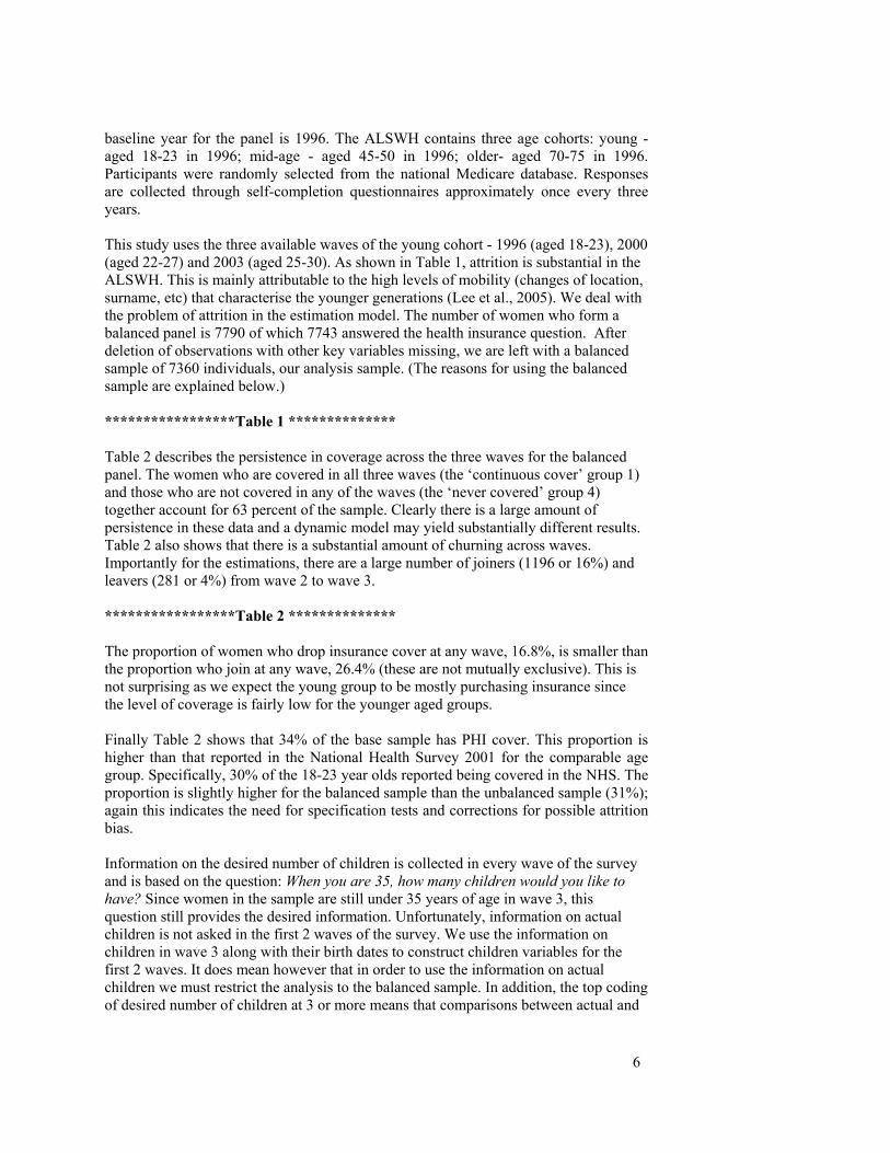
baseline year for the panel is 1996. The ALSWH contains three age cohorts: young - aged 18-23 in 1996; mid-age - aged 45-50 in 1996; older- aged 70-75 in 1996. Participants were randomly selected from the national Medicare database. Responses are collected through self-completion questionnaires approximately once every three years. This study uses the three available waves of the young cohort - 1996 (aged 18-23), 2000 (aged 22-27) and 2003 (aged 25-30). As shown in Table 1, attrition is substantial in the ALSWH. This is mainly attributable to the high levels of mobility (changes of location, surname, etc) that characterise the younger generations (Lee et al., 2005). We deal with the problem of attrition in the estimation model. The number of women who form a balanced panel is 7790 of which 7743 answered the health insurance question. After deletion of observations with other key variables missing, we are left with a balanced sample of 7360 individuals, our analysis sample. (The reasons for using the balanced sample are explained below.) *****************Table 1 ************** Table 2 describes the persistence in coverage across the three waves for the balanced panel. The women who are covered in all three waves (the ‘continuous cover’ group 1) and those who are not covered in any of the waves (the ‘never covered’ group 4) together account for 63 percent of the sample. Clearly there is a large amount of persistence in these data and a dynamic model may yield substantially different results. Table 2 also shows that there is a substantial amount of churning across waves. Importantly for the estimations, there are a large number of joiners (1196 or 16%) and leavers (281 or 4%) from wave 2 to wave 3. *****************Table 2 ************** The proportion of women who drop insurance cover at any wave, 16.8%, is smaller than the proportion who join at any wave, 26.4% (these are not mutually exclusive). This is not surprising as we expect the young group to be mostly purchasing insurance since the level of coverage is fairly low for the younger aged groups. Finally Table 2 shows that 34% of the base sample has PHI cover. This proportion is higher than that reported in the National Health Survey 2001 for the comparable age group. Specifically, 30% of the 18-23 year olds reported being covered in the NHS. The proportion is slightly higher for the balanced sample than the unbalanced sample (31%); again this indicates the need for specification tests and corrections for possible attrition bias. Information on the desired number of children is collected in every wave of the survey and is based on the question: When you are 35, how many children would you like to have? Since women in the sample are still under 35 years of age in wave 3, this question still provides the desired information. Unfortunately, information on actual children is not asked in the first 2 waves of the survey. We use the information on children in wave 3 along with their birth dates to construct children variables for the first 2 waves. It does mean however that in order to use the information on actual children we must restrict the analysis to the balanced sample. In addition, the top coding of desired number of children at 3 or more means that comparisons between actual and
7
desired numbers cannot be made for those women with both 3 or more actual and 3or more desired children. These women constitute a small fraction of the balanced sample (2% of observations). We include these observations in the analysis and add a dummy variable which equals 1 when the comparison between desired and actual children cannot be determined. Information on current pregnancy is collected in all waves of the survey. We use this information as a measure of the timing of the desired children; pregnant women who desire additional children want them in the immediate future rather than much later in life.2 Due to waiting periods in most insurance contracts, women must purchase insurance before the beginning of pregnancy in order to be covered at the time of childbirth. *****************Table 3 ************** Table 3 provides frequencies of desired and actual children, pregnancies and private insurance cover for the balanced sample of 22080 observations (7360 individuals over 3 waves). 19% of the observations in the balanced sample consist of women who have children. The incidence of pregnancies is not that high (6%) but given the large sample sizes, it still includes a substantial number of observations (1371 observations). In the raw data, women with children are less likely to have private health insurance than women without children (29% versus 38%). Marital status is included with a series of dummy variables: married or defacto (43% of the sample of observations), single (55% of observations), separated or divorced (2% of observations). We include several other factors in the model of insurance. These have been identified as important determinants of insurance demand in previous studies. We briefly describe the additional regressors next and a full list with definitions is given in Appendix 1. It is shown in many previous studies that private health insurance holders have a higher income distribution than those without cover (Perry and Rosen, 2001). This also holds for the data set under study (Salale, 2006). Insurance is generally found to be a normal good and the current government incentive structure in Australia intensifies this relationship. The ALSWH collects information on personal and household weekly income. Income is measured in 8 categories with the top category corresponding to 1500AUD per week or an annual income of 78,000. Dummy variables are used to capture variations in the income categories. As discussed above, we expect the income effect to vary depending on actual and desired children due to changes in equivalent household income, savings motive and risk aversion. Specifications of the insurance model are estimated with interactions of income and the children variables. Unfortunately, income was not asked in the first wave of the survey. This does not affect the dynamic model estimation as the likelihood is conditional on the initial 2 It is possible that pregnant women count unborn children as actual children. We cannot determine how women interpret the question on actual children by looking at the data. There are pregnant women in the sample who do not desire any additional children but this could be an indication of unwanted pregnancy. We do not want to rule out unwanted pregnancies by redefining the children variables in these cases.
8
conditions and the first wave information on variables other than insurance is not used. (See below for a detailed discussion of the model.) The missing wave 1 income information does however affect the attrition correction for the pooled probit specification. We discuss this further below. A dummy for missing income is also included for missing values in waves 2 and 3 (6% of observations for personal income and 21% for household income). The existence of adverse selection in an insurance industry generates a positive correlation between risk and insurance choice [Chiappori and Salanie (2000), Cutler and Zeckhauser (1999)]. However, recent studies show that this relationship may be difficult to capture due to heterogeneity in risk aversion (Finkelstein and McGarry (2003)). Doiron, Jones and Savage (2006) find a negative correlation between risk (as measured by self-assessed health) and the choice to insure in cross-sectional Australian data. They also find that the positive relationship predicted by adverse selection is recovered when measuring risk with chronic conditions. Based on risk-related behaviours, they find evidence that the counterintuitive negative correlation is due to the effect of heterogeneous risk aversion as measured by risk-related behaviours. Self assessed health is available in all waves of the survey and is used in the estimation of the insurance model. There is also information on long-term conditions but the numbers of women with any type of long term condition (bar asthma) is never above 3 percent of the sample in each wave (Salale, 2006). Hence the scope for an analysis of the effects of chronic conditions on insurance among this age group is limited. We include a variable measuring the number of reported long-term conditions without specifying the nature of the illnesses. We also include variables measuring risk-related behaviours (smoking, BMI, alcohol consumption and exercise). The ALSWH data set also measures women’s perception of access to health care services. For the purposes of this study perception of hospital access is an important and usually unmeasured variable. Using a bivariate analysis of the relationship between income and self-reported access, Salale (2006) shows access to hospitals may be inequitable. This follows from women with lower incomes and no hospital insurance reporting lower access levels, while women with higher incomes and hospital insurance are more likely to report the opposite. Access to care relates to either public or private care. Since private hospitals are more unevenly distributed across geographical areas, this variable is an important indicator of the usefulness of private insurance and is included in the analysis. Additional explanatory variables measuring socio-economic status (education, employment status), geographical location (state dummies, degree of remoteness) and country of birth are included. (Please see Appendix 1 for more details.) 4 MODEL SPECIFICATION Most estimates of the demand for insurance are based on cross-section variations although one would expect the demand for insurance to have an important dynamic component. As summed up by Propper (1989, p791), “[…] captivity and the effect of past purchase would be promising avenues to explore”. Individuals may not revisit the decision to purchase health insurance every year and there are costs associated with
9
moving in and out of the market (e.g. the age penalty in the premiums legislated by government, and waiting times for claims). Panel or retrospective data are needed for these models and until recently such data were still rare in health. The use of dynamic models in the context of insurance and indeed for most health-related variables is complicated by the need to use nonlinear models able to accommodate discrete endogenous variables. We follow recent approaches in modelling the demand for insurance as a dynamic probit regression assuming a first-order Markov process for the dynamic effect [Contoyannis, Jones and Rice (2004); Arulampalam, Booth and Taylor (2000); Erdem and Sun (2001)] such that only the most recent information is relevant in the choice decision. Specifically, the demand for health insurance can be written as:
PHI it* = X it β�γ PHI i ,t−1�Z it× PHIi ,t−1��uit i= 1,2, .. . ,N t= 1,. .. ,Ti (1)
⎭⎬⎫
⎩⎨⎧ >
=otherwise ,0
]0[ , 1 *it
itPHI
PHI
where *PHI is a latent variable measuring the net benefits of private health insurance;
PHI is the observed insurance status (insurance is purchased only when the net benefits of insurance are positive); the vector Xit represents observable, exogenous variables that affect insurance choice (it does not include a constant term); PHIi,t-1 is a lag of the dependent variable capturing the effect of state dependence; the vector Zit includes a subset of the X variables that are interacted with the lagged insurance status; N indicates the number of individuals in the panel; T is the number of periods in the panel which can be individual specific in the case of the unbalanced sample; uit is a composite error term which is explained further below. The use of panel data allows us to control for the presence of individual specific and time-invariant effects at least partially unobserved. In dynamic models, these can be crucial since their omission will lead to overestimation of the dynamic effects; ignoring individual effects leaves the dynamic effects as the only source of correlation across time periods (in the absence of serial correlation). We follow recent empirical papers in specifying random correlated effects where individual-specific effects have a random component independent of the explanatory variables and a deterministic component which is a linear function of the explanatory variables (or functions thereof). This is the approach used in Contoyannis, Jones and Rice (2004) and Arulampalam, Booth and Taylor (2000) and is based on work by Chamberlain (1984) and Mundlak (1978). Specifically, the composite error uit is specified as:
itiit au ε+= (2) where ai is an individual-specific, time-constant random term drawn from a normal distribution and εit is a time-varying, individual specific random error. Under the probit specification, εit is normally distributed with a variance normalised to 1. Following Mundlak (1978), the unobservable individual effect, ai, and the exogenous variables are related in a linear manner,
iiia ηα ++= Xα10 (3) where iX is a vector of means of any time-varying regressors and ηi is a normally distributed random error term assumed to be independent of X.
1
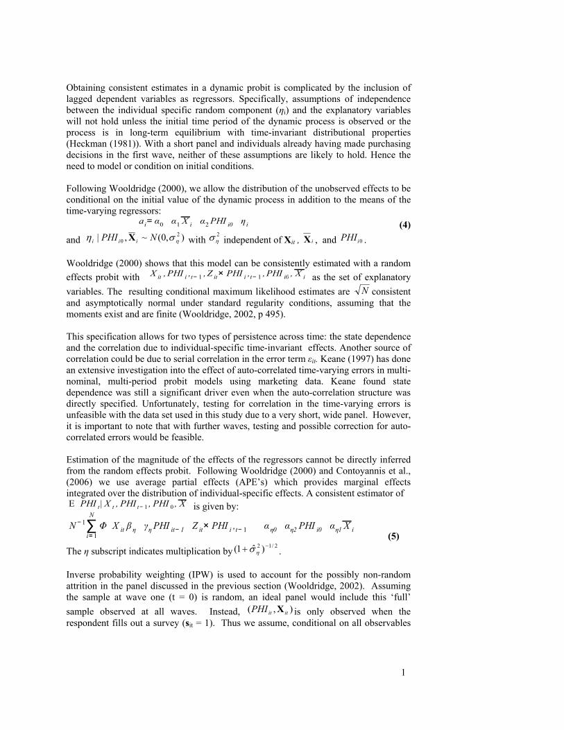
Obtaining consistent estimates in a dynamic probit is complicated by the inclusion of lagged dependent variables as regressors. Specifically, assumptions of independence between the individual specific random component (ηi) and the explanatory variables will not hold unless the initial time period of the dynamic process is observed or the process is in long-term equilibrium with time-invariant distributional properties (Heckman (1981)). With a short panel and individuals already having made purchasing decisions in the first wave, neither of these assumptions are likely to hold. Hence the need to model or condition on initial conditions. Following Wooldridge (2000), we allow the distribution of the unobserved effects to be conditional on the initial value of the dynamic process in addition to the means of the time-varying regressors:
ai= α0�α1 X i�α2 PHI i0�η i (4) and ),0(~,| 2
0 ηση NPHI iii X with 2ησ independent of Xit , iX , and 0iPHI .
Wooldridge (2000) shows that this model can be consistently estimated with a random effects probit with �X it , PHI i ,t− 1 , Z it× PHI i ,t− 1 ,PHI i0 , X i�as the set of explanatory variables. The resulting conditional maximum likelihood estimates are N consistent and asymptotically normal under standard regularity conditions, assuming that the moments exist and are finite (Wooldridge, 2002, p 495). This specification allows for two types of persistence across time: the state dependence and the correlation due to individual-specific time-invariant effects. Another source of correlation could be due to serial correlation in the error term εit. Keane (1997) has done an extensive investigation into the effect of auto-correlated time-varying errors in multi-nominal, multi-period probit models using marketing data. Keane found state dependence was still a significant driver even when the auto-correlation structure was directly specified. Unfortunately, testing for correlation in the time-varying errors is unfeasible with the data set used in this study due to a very short, wide panel. However, it is important to note that with further waves, testing and possible correction for auto-correlated errors would be feasible. Estimation of the magnitude of the effects of the regressors cannot be directly inferred from the random effects probit. Following Wooldridge (2000) and Contoyannis et al., (2006) we use average partial effects (APE’s) which provides marginal effects integrated over the distribution of individual-specific effects. A consistent estimator of E �PHI t | X t , PHI t− 1 , PHI 0 , X �is given by:
N −1∑i= 1
N
Φ�X it�βη��γηPHI it− 1�Z it× PHI i ,t− 1
���� �αη0� �αη2 PHI i0� �αη1 X i � (5)
The η subscript indicates multiplication by2/12 )ˆ1( −+ ησ .
Inverse probability weighting (IPW) is used to account for the possibly non-random attrition in the panel discussed in the previous section (Wooldridge, 2002). Assuming the sample at wave one (t = 0) is random, an ideal panel would include this ‘full’ sample observed at all waves. Instead, ),( ititPHI X is only observed when the respondent fills out a survey (sit = 1). Thus we assume, conditional on all observables
1
in the first time period (labelled here 1iZ ), ititPHI X, are independent of the response sit such that,
TtPPHIP iitiititit ,...,2 ),|1(),,|1( 11 ==== ZsZXs (4.14) To implement IPW, two steps are used. Firstly, for each time period a binary probit is estimated measuring )|1( 1iit zsP = , and a fitted probability itp̂ is gained for each unit. Secondly, the pooled probit is weighted by itp̂/1 so that a greater weighting is placed on observations of units with a lower response rate. Wooldridge (2002) shows that IPW produces consistent, N -asymptotically normal estimators. This is the approach followed in Contoyannis et al (2006). In this paper, we estimate the insurance models on the balanced sample hence, we must estimate the probability of being in the sample in every year. Usint the previous notation, (sit = 1) only if the individual is in the balanced sample. Wooldridge (2002) shows that this method yields consistent, N -asymptotically normal estimators in models where the likelihood can be written as a sum of contributions across all observations. This is not the case when individual-specific random effects are present. The correction for attrition is performed on pooled probit models only. This is also the approach followed in Contoyannis et al (2005). For missing exogenous variables in time periods other than the initial period, dummy variables are used. As the panel is a short, wide panel, a set of time dummies is needed – therefore a dummy for the year 2000 is included (Wooldridge 2002, p 484) in all the random effects probit models. As described above, this dummy variable will also capture advertising effects surrounding the life-time cover reform of 2000. 5 RESULTS Specification Equation (1) is estimated with both pooled probits and random effects probits on observations for waves 2 and 3. Wave 1 observations are used in specifying the initial conditions for PHI. Various specifications are estimated. The main model on which most of the results are based includes the following variables for X: lagged PHI cover, initial PHI cover, actual and desired children variables, marital status, household income, single income household dummy, left home since last wave dummy, age, self-assessed health, health card dummy, queensland dummy, rural and remote area dummies, education, risk-related variables (smoking, alcohol, bmi, bmi if pregnant, exercise), country of birth, study and work status, access to health services dummies. Means of household income dummies are used in the correlated random effects and interactions of actual and desired children variables with lagged PHI cover are included in the Z variables. Separate models estimated for women with and without children yield very similar results to the specifications with interactions of children and lagged PHI variables only. Personal income dummies are not significant when household income dummies are included. Also including the mean personal income dummies in the correlated random effects yields results that are not statistically different from those with only mean household income variables. Random effects specifications yield very similar results to the pooled dynamic probit models although formal tests lead rejections of the pooled models in favour of the random effects specification. This is similar to the results in Contoyannis et al (2005) in the context of dynamic models of health. Given the relative simplicity and speed of
1
estimation of the pooled probits compared to the random effects specification, many of the models presented below are estimated with pooled probit specifications. In all specifications, significance tests on the lagged dependent variable yield strong rejections of the static specification in favour of the dynamic model. There is substantial persistence in insurance cover and the lagged PHI variable is better at capturing the correlation over time than the random effects. Finally, joint tests of the significance of the mean household income dummies yield strong rejections of the simple random effects model in favour of the correlated specification.
Effects of actual and desired children variables Tables 4 to 6 describe the effects of actual and desired children on the predicted probability of private insurance cover. Table 4 presents the predicted probabilities and differences (marginal effects) based on the dynamic pooled probit specification. Table 5 presents the predicted probabilities and differences (average partial effects) for the dynamic correlated random effects probit. Finally Table 6 presents corresponding results for a specification which includes interactions between children variables, lagged insurance and the currently pregnant dummy variable (only the results for those without insurance in the previous period are presented). Beginning with Table 4 and focusing on those without insurance in wave 2, we find that women who desire more children are more likely to purchase insurance. The effect is quantitatively large and significant at 6 percentage points. Also this effect is similar whether or not these women have children. Women who have children are less likely to join, again the effect is around 6 ppt and significant. It is similar for those women who desire more children and for those who have finished their family. Looking at women who did have insurance in the previous period allows us to look at the decision to drop insurance. The desire for more children does not significantly affect the probability of dropping insurance conditioning on the presence of children. Women with children are less likely to drop insurance cover than those without children. The effect is around 3 ppt and is marginally significant. It is found only for those who desire more children. Table 5 shows similar quantitative and qualitative results for the random effects specifications. Table 6 shows that women who are currently pregnant are more likely to have joined insurance between the 2 periods compared to similar women who are not pregnant. (The interactions with the currently pregnant dummy are not significant possibly due to the small number of observations.) These results suggest that insurance benefits surrounding pregnancy and childbirth are highly valued by women. Benefits of insurance for children are less valuable and are dominated by income effects caused by the presence of chidren.
1
REFERENCES Arulampalam., W., Booth., A., Taylor., M., (2000) Unemployment Persistence. Oxford Economic Papers, 52 (1), 24-50 Asinski,D., (2005) Health Insurance, Access to Care and Risk-Aversion: Separating Selection and Incentive Effects. Working paper, November Australian Bureau of Statistics [ABS] (2001) National Census 2001: Population Tables by Age and Sex. Electronic delivery: data cube: Cat. No. 3235.0.55.001. Viewed 1 October 2006. Australian Bureau of Statistics [ABS] (2001) National Health Survey 2001. Canberra, Australia. Australian Bureau of Statistics [ABS] (2005) National Health Survey 2004 -05. Canberra, Australia. Australian Bureau of Statistics [ABS] (1995) National Health Survey 1995. Canberra, Australia. Australian Government. Private Health Insurance Incentives Act 1998 (Act No. 121), Attorney-General’s Department, Canberra. Barrett, G., Conlon, R., (2003) Adverse selection and the contraction in the market for private health insurance: 1989-1995. The Economic Record, 79 (246), 279-296 Bell, S., (2002) Data book for the 2000 Phase 2 survey of the young cohort (22-27 years) Australian Longitudinal Study on Women’s Health. The Research Centre for Gender and Health, University of Newcastle, NSW Australia. January, 2002 Butler, J.R.G., (2001) Policy change and private health insurance: Did the cheapest policy do the trick? NCEPH Working Paper Number 44. The Australian National University. Butler, J., Moffitt, R., (1982) A Computationally Efficient Quadrature Procedure for the One Factor Multinomial Probit Model. Econometrica, 50, p761-764 Cameron, A.C, Trivedi, P.K., Milne, F., Piggott, J., (1998) A Microeconometric Model of the Demand for Health Care and Health Insurance in Australia. Review of Economic Studies, 55 (1), 85-106 Card D., C. Dobkin and N. Maestas (2004), The Impact of Nearly Universal Insurance
Coverage on Health Care Utilization and Health: Evidence from Medicare, NBER Working Paper 10365, March, 74 pgs.
Ettner S.L. (1997), “Adverse selection and the purchase of Medigap insurance by the
elderly”, Journal of Health Economics, 16, 543–562.
Comment: Fix these references
Comment: Fix these references
Comment: Fix these references
1
Cardon, J., Hendel, I., (2001) Asymmetric information in health insurance: evidence from the National Medical Expenditure Survey. RAND Journal of Economics, 32 (3), 408-427 Case, A., Lubotsky, D., Paxson, C., (2002) Economic Status and Health in Childhood: the Origins of the Gradient. The American Economic Review, 92 (5), 1308-1334 Centrelink (Site Date: 13/03/2006) Health Care Cards. Viewed on 21 Oct, 2006. <http://www.centrelink.gov.au/internet/internet.nsf/payments/conc_cards_hcc.htm> Chamberlain, G., (1984) Panel Data. S. Griliches and M. Intriligator (eds) Handbook of Econometrics, Amsterdam, North-Holland, 1247-1318 Chiappori, P.A, Salanie, B., (2000) Testing for Asymmetric Information in Insurance Markets. The Journal of Political Economy, 108 (1), 56-78 Contoyannis, P., Jones, A., Rice, N., (2004) The Dynamics of Health in the British Household Panel Survey. Journal of Applied Econometrics, 19, 473-503 Cutler, D., Zeckhauser, R., (1999) The Anatomy of Health Insurance. NBER working paper 7176 Cutler, H., Fiebig, D., (2005) The demand for private health insurance allowing for substitution. Working paper, 16 September, 2005 Doiron, D., Jones, G., Savage, E., (2006) Healthy, Wealthy and Insured? The Role of Self-Assessed Health in the Demand for Private Health Insurance. Working paper, September. Erdem, T., Sun, B., (2001) Testing for choice dynamics in panel data. Journal of Business and Economic Statistics, 19, 142-152 Fang, H., Keane, M., Silverman, D., (2005) Sources of Advantageous Selection: Evidence from the Medigap Insurance Market. Working Paper, November 28 Finkelstein, A., McGarry, K., (2003) Private Information and its Effect on Market Equilibrium: New Evidence from Long-Term Care Insurance. NBER Working Paper 9957, September. Fitzgerald, J, Gottschalk, P, Moffitt, R (1998) An Analysis of Sample Attrition in Panel Data: The Michigan Panel Study of Income Dynamics. The Journal of Human Resources, 33 (2), 251-299 Frech III, H.E, Hopkins, S., (2004) Why Subsidise Private Health Insurance? The Australian Economic Review, 37 (3) p 243-56 Frech III, H.E, Hopkins, S., Macdonald, G., (2003) The Australian private health insurance boom: was it subsidies or liberalized regulation? Economic Papers, 22 (1) p 58-64
1
Gans, J., King, S., (2003) Anti-insurance: Analysing the Health Insurance System in Australia. The Economic Record, 79 (247), 473-486 Gardiol, L., Geoffard, P-Y., Grandchamp, C., (2005) Separating selection and incentive effects in health insurance. Working Paper 2005-38, Paris-Jourdan Sciences Economiques Greene, W., (2003) Econometric Analysis, 5th Ed. Pearson Education, New Jersey, USA Grossman, M., (1972) On the Concept of Health Capital and the Demand for Health. The Journal of Political Economy, 80 (2), 223-255. Hall, J., (2004) Can We Design a Market for Competitive Health Insurance? CHERE Discussion Paper 53, February 2004. Hall, J., de Abreu Lourenco, R., Viney, R., (1999) Carrots and Sticks – The Fall and Fall of Private Health Insurance in Australia. Health Economics, 8, 653-660. Health Insurance Commission [HIC] (2003) Annual Report. Australian Government Publishing Services, Canberra. Heckman, J.J., (1981) The incidental parameters problem and the problem of initial conditions in estimating a discrete time-discrete data stochastic process, in C F Manski and D McFadden (eds.), Structural Analysis of Discrete Data with Econometric Applications, MIT Press, Cambridge, MA, 114-78 HICA Health (2006) Regulation of Private Health Insurance. Available at http://hica.com.au/govphiregulation.html. Accessed 30 Oct, 2006. Hopkins, S., Kidd, M.P., (1996) The determinants of the demand for private health insurance under Medicare. Applied economics, 28, 1623-1632 Hurley, J., Vaithianathan, R., Crossley, T. and Cobb-Clark, D. (2001), Private parallel health insurance in Australia: A cautionary tale and lessons for Canada, Working paper no. 01-12, Centre for Health Economics and Policy Analysis, McMaster University. Hyslop, D., (1999) State Dependence, Serial Correlation and Heterogeneity in Intertemporal Labour Force Participation of Married Women. Econometrica, 67 (6), 1255-1294 Keane, M., (1997) Modelling Heterogeneity and State Dependence in Consumer Choice Behaviour. Journal of Business and Economic Statistics, 15 (3), 310-327 Kennedy, P., (2003) A Guide to Econometrics, Fifth Edition. The MIT Press, Cambridge, Massachusetts.
1
Lee, C., Dobson, A., Brown, W., Bryson, L., Byles, J., Warner-Smith, P., Young, A., (2005). Cohort Profile: The Australian Longitudinal Study on Women’s Health. International Journal of Epidemiology, 34, 987-991. Manning, W., J. Newhouse, N. Duan, E. Keeler, A. Leibowitz, and M. Marquis. (1987) “Health Insurance and the Demand for Medical Care: Evidence from a Randomized Experiment”, American Economic Review, 77, 251-277. Mishra, G., Schofield, M., (1998) Norms for the physical and mental health component summary scores of the SF-36 for young, middle and older Australian women. Quality of Life Research, 7 (3), 215-220. Mundlak, Y., (1978) On the Pooling of Time Series and Cross Section Data. Econometrica, 46, 69-85 Orme, C., (1997) The initial conditions problem and two-step estimation in discrete panel data models, mimeo, Department of Economics, University of Manchester, Manchester Palangkaraya, A., Yong, J. (2005) “Effects of Recent Carrot-and-Stick Policy Initiatives on Private Health Insurance Coverage in Australia”, The Economic Record, 81(254) September, 262-72. Parliament of Australia (2006), Bills Digest no. 148, 2005-06, Tax Laws Amendment (Medicare Levy and Medicare Levy Surcharge) Bill 2006. Pauly, M., Zheng, Y., (2003) Adverse Selection and the Challenges to Stand-Alone Prescription Drug Insurance. Working Paper 9919, National Bureau of Economic Research, Cambridge Perry CW, Rosen HS (2001) The Self-Eemployed are Less Likely to Have Health Insurance Than Wage Earners. So What? NBER Working Paper 8316. National Bureau of Economic Research: Cambridge. Powers, J., (2004) Comparison of the Australian Longitudinal Study on Women’s Health Cohort’s with women of the same age in the 2001 Census. Technical Report; Women’s Health Australia. Private Health Insurance Ombudsman [PHIO] (2005) State of the Health Funds Report, 2005. Australian Government, Canberra. Propper, C., (1989) An econometric analysis of the demand for private health insurance in England and Wales. Applied Economics, 21, 777-792 Rothschild, M., and Stiglitz, J., (1976) Equilibrium in Competitive Insurance Markets: An Essay on the Economics of Imperfect Information. Quarterly Journal of Economics 90, 629-49
1
Roy, R., Chintagunta, P., Halder, S., (1996) A Framework for Investigation Habits, “The Hand of the Past”, and Heterogeneity in Dynamic Brand Choice. Marketing Science, 15 (3), 280-299 Salale, V., (2006) Modelling Dynamic Choice: Private Health Insurance in Australia. CHERE Research Report 24, CHERE, Sydney Savage, E., and Wright, D., (2003) Moral Hazard and adverse selection in Australian private hospitals: 1989-1990. Journal of Health Economics 22, 331-359 Scotton, R. (1999). Managed competition in Mooney, G., Scotton, R. Economics and Australian Health Policy. Sydney, Allen & Unwin: 214-231. Scotton, R. B. (1990). Integrating Medicare with private health insurance: The best of both worlds? in Selby Smith, C. Economics and Health 1989: Proceedings of the Eleventh Australian Conference of Health Economists. Clayton, Monash University: 219-38. Stewart, M., (2006) Maximum Simulated Likelihood Estimation of Random Effects Dynamic Probit Models with Autocorrelated Errors. Working Paper, University of Warwick, April. The Private Health Insurance Administration Council (PHIAC) (2006) Coverage of Hospital Insurance Tables. Available at http://www.phiac.gov.au/statistics/membershipcoverage/hosquar.htm The Private Health Insurance Administrations Council (PHIAC) (2005) Operations of the Registered Health Benefits Organisations, Annual Report 2004-05. Commonwealth of Australia. Vaithianathan, R., (2004) A Critique of the Private Health Insurance Regulations. Australian Economic Review, 37 (3), 257-270 Viney, R., Savage, E., Fiebig, D., (2006) Does the reason for buying health insurance influence behaviour? CHERE Working Paper, University of Technology, 2006 Wooldridge, J., (2002) Econometric Analysis of Cross Section and Panel Data. The MIT Press, Cambridge Massachusetts Wooldridge, J., (2003) Introductory Econometrics: A Modern Approach, Second Edition. Thomson South-Western, United States of America. Wooldridge, J., (2005) Simple Solutions to the Initial Conditions Problem in Dynamic, Nonlinear Panel Data Models with Unobserved Heterogeneity. Journal of Applied Econometrics, 20, 39-54
1
APPENDICES Appendix 1: Variable definitions
Variable Name Definition Private Insurance Choice PHI PHIi,t-1 PHIi0
= 1 if hold private hospital insurance in the current period, 0 otherwise = 1 if held private hospital insurance in the previous period, 0 otherwise = 1 if hold private hospital insurance in 1996, 0 otherwise
Year Y2000
= 1 if year is 2000, 0 otherwise
Personal income INC1 INC2 INC3 INC4 INC5 INC6 INC7 INC8 INCMISS
= 1 if respondent earns no income, 0 otherwise = 1 if respondent earns $1-$199pw, 0 otherwise = 1 if respondent earns $120-$299pw, 0 otherwise = 1 if respondent earns $300-$499pw, 0 otherwise = 1 if respondent earns $500-$699pw, 0 otherwise = 1 if respondent earns $700-$999pw, 0 otherwise = 1 if respondent earns $1000-$1499pw, 0 otherwise = 1 if respondent earns $1500+ pw, 0 otherwise = 1 if Missing/Don’t want to answer, 0 otherwise
= 1 if household earns no income, 0 otherwise = 1 if household earns $1-$199pw, 0 otherwise = 1 if household earns $120-$299pw, 0 otherwise = 1 if household earns $300-$499pw, 0 otherwise = 1 if household earns $500-$699pw, 0 otherwise = 1 if household earns $700-$999pw, 0 otherwise = 1 if household earns $1000-$1499pw, 0 otherwise = 1 if household earns $1500+ pw, 0 otherwise = 1 if Missing/Don’t want to answer, 0 otherwise = 1 if respondent lives alone, 0 otherwise
AGE = Age of respondent (years) LVHOME = 1 if respondent left family home in past 12 months, 0 otherwise Employment Status STUDY WORK WORKSTUDY NOWORKSTUDY WORKMISS
= 1 if study but not work, 0 otherwise = 1 if work but not study, 0 otherwise = 1 if work and study, 0 otherwise = 1 if don’t work or study, 0 otherwise = 1 if work/study status is missing, 0 otherwise
= 1 if completed tertiary qualifications, 0 otherwise = 1 if completed a diploma, 0 otherwise = 1 if completed other qualifications, 0 otherwise = 1 if only primary or secondary schooling, 0 otherwise = 1 if qualification is missing, 0 otherwise
State NSW VIC QLD SA WA TAS NT ACT STATEMISS
= 1 if lives in New South Wales, 0 otherwise = 1 if lives in Victoria, 0 otherwise = 1 if lives in Queensland, 0 otherwise = 1 if lives in South Australia, 0 otherwise = 1 if lives in Western Australia, 0 otherwise = 1 if lives in Tasmania, 0 otherwise = 1 if lives in Northern Territory, 0 otherwise = 1 if lives in Australian Capital Territory, 0 otherwise = 1 if state of residence missing, 0 otherwise
Area URBAN RURAL REMOTE AREAMISS
= 1 if lives in a major urban area, 0 otherwise = 1 if lives in a rural area, 0 otherwise = 1 if lives in remote area, 0 otherwise = 1 if area of residence is missing
1
Appendix 2: Variable means and standard deviations
* indicates the omitted category from a group of dummy variables
TABLES
2
Table 1: Sample sizes for the young cohort, ALSWH
Wave 1: 1996 Wave 2: 2000 Wave 3: 2003 Age of women 18 – 23 22 – 27 25 – 30 Retention rates 100% (N = 14,779) 66% (N = 9,690) 61% (N = 9,074) Panel respondents 96% (N = 14,247) 66% (N = 9,688) 53% (N = 7,790) Response recorded for the private hospital insurance question
95% (N = 14,070) 64% (N = 9,528) 52% (N = 7,743)
Table 2: Private health insurance cover, balanced panel
Group Wave 1: 1996
Wave 2: 2000
Wave 3: 2003
No of women %
1 ‘Continuous cover’ Y Y Y 1398 19.0 2 ‘Recent leaver’ Y Y N 166 2.3 3 ‘Leaver’ Y N N 599 8.1 4 ‘Never covered’ N N N 3252 44.2 5 ‘New joiner’ N N Y 839 11.4 6 ‘Joiner’ N Y Y 634 8.6 7 ‘Churn out’ N Y N 115 1.6 8 ‘Churn in’ Y N Y 357 4.9 Total 7360 100.0 % with insurance cover 34% 31% 44% 36.5% Table 3: Children variables and private health cover (obs=22080) Have Children No Children Total Balanced Sample 4270 17810
Desired > Actual 2679 63% 15320 86% Desired ≤ Actual 1146 27% 2490 14%
Indeterminate* 445 10% Currently Pregnant:
Desired > Actual 628 15% 538 3% Desired ≤ Actual 107 3% 28 <1%
Insured: Desired > Actual 866 20% 6010 34% Desired ≤ Actual 277 6% 816 5%
*Desired and actual numbers of children are equal to or greater than 3.
2
Table 4: Children variables and average predicted probability of cover – pooled probits (observations=22080)1
No kids With kids Difference (p-value) Not insured in t-1
Desired > Actual 0.283 0.220 0.063* (0.000) Desired ≤ Actual 0.227 0.162 0.065* (0.002)
Was insured in t-1 Desired > Actual 0.715 0.749 -0.034** (0.097) Desired ≤ Actual 0.737 0.723 0.014 (0.708)
Difference -0.022 0.026 (p-value) (0.342) (0.455)
1p-values based on tests on the underlying coefficients. P-values on the marginal/average partial effects still to be computed. *indicates significance at 1% **indicates significance at 10%. Table 5: Children variables and average predicted probability of cover – random effects probits (observations=22080)1
No kids With kids Difference (p-value) Not insured in t-1
Desired > Actual 0.311 0.256 0.055* (0.000) Desired ≤ Actual 0.259 0.199 0.060* (0.006)
Was insured in t-1 Desired > Actual 0.599 0.631 -0.032 (0.148) Desired ≤ Actual 0.620 0.595 0.025 (0.583)
Difference -0.021 0.036 (p-value) (0.432) (0.349)
1p-values based on tests on the underlying coefficients. P-values on the marginal/average partial effects still to be computed. *indicates significance at 1% **indicates significance at 10%.
2
Table 6: Children variables,pregnancy and average predicted probability of cover – pooled probits (observations=22080)1
Not insured in t-1 No kids With kids Difference (p-value) Currently pregnant
Desired > Actual 0.286 0.237 0.049 (0.130) Desired ≤ Actual 0.182 0.182 0.000 (0.997)
Difference 0.104 0.055 (p-value) (0.222) (0.376)
Not pregnant Desired > Actual 0.279 0.216 0.063* (0.000) Desired ≤ Actual 0.224 0.158 0.066* (0.003)
1p-values based on tests on the underlying coefficients. P-values on the marginal/average partial effects still to be computed. *indicates significance at 1% **indicates significance at 10%.


![[On-Demand Webinar] What is Landlord Insurance?](https://static.documents.pub/doc/80x56/58ed28111a28ab440e8b460f/on-demand-webinar-what-is-landlord-insurance.jpg)


