Family Size, Sibling Rivalry and Migration:

Evidence from Mexico∗

Massimiliano Bratti† Simona Fiore‡ Mariapia Mendola§

May 20, 2016

Abstract

This paper examines the effects of family size and demographic structure on off-spring’s international migration. We use rich survey data from Mexico to estimate theimpact of sibship size, birth order and sibling composition on teenagers’ and youngadults’ migration outcomes. We find little evidence that high fertility drives migration.The positive correlation between sibship size and migration disappears when endogene-ity of family size is addressed using biological fertility (miscarriages) and infertilityshocks. Yet, the chances to migrate are not equally distributed across children withinthe family. Older siblings, especially firstborn males, are more likely to migrate, whilehaving more sisters than brothers may increase the chances of migration, particularlyamong girls. [JEL codes: J13 F22 O15.]

Keywords: International Migration, Mexico, Family Size, Birth Order, Sibling Com-position.

∗We thank Catia Batista, Pascaline Dupas, Ivan Etzo, Margherita Fort, Marco Mantovani, Maria Perrotta,Pedro Rosa Dias, Jenny Simon, Giancarlo Spagnolo, Shqiponja Telhaj, Pedro Vicente, Alan Winters, andseminar audiences at University of Sussex, SITE–Stockholm School of Economics, Nova School of Businessand Economics (Lisbon), University of Bologna, University of Turin, University of Milano-Bicocca, RoyalEconomic Society Conference (Brighton), ESPE Conference (Izmir) and SIE Conference (Naples) for usefulcomments and discussions. The usual disclaimer applies.†Università degli Studi di Milano and IZA, massimiliano.bratti@unimi.it‡Università degli Studi di Bologna, simona.fiore3@unibo.it§Corresponding author. Università degli Studi di Milano–Bicocca and IZA, mariapia.mendola@unimib.it

1

1 Introduction

Migration from poor to rich countries is one of the most important ways through which

workers can increase their income opportunities as well as their families’ welfare back home

(Chen et al. 2003, Kennan and Walker 2011, Clemens 2011). A key feature of migration is

that it mainly involves young adults who are more likely to have a positive net expected return

to migration due to their longer remaining life expectancy (Sjaastad 1962). According to

recent UN figures, worldwide international migrants aged 15 to 24 account for 12.5 per cent

of total migrants worldwide, and when migrants between the ages of 25 and 34 are added,

young migrants represent over 30 per cent of the total (UNDESA 2011). The proportion of

youth migrants is much higher in developing countries than it is in advanced countries and it

more than doubles if we consider internal migrants as well (UN 2013).

Given the profitable nature of labor mobility, which involves both the (young) migrant

and her origin family, an extensive literature on the determinants of migration has empha-

sized the important role of household (along with individual) factors in the migration deci-

sion (e.g. Rosenzweig and Stark 1989, Stark 1991). Indeed, in many developing countries,

labor migration is a family strategy to diversify income sources, improve earning potentials

and increase household security through remittances (e.g. Stark and Bloom 1985, Yang 2008,

Antman 2012).

As a result, family migration strategies in developing contexts may involve the costly

parental decision to dispatch one of the children to work in a different city or abroad, and

to invest in a potentially remitting child (Lucas and Stark 1985, Jensen and Miller 2011).

However, parents face a number of trade-offs when allocating resources across their children,

due to either limited household resources or (perceived) different returns on the migration

investment (e.g., son bias).1 This may generate resource dilution effects in large families

or competition (rivalry) among siblings from the same household (Garg and Morduch 1998,

Black et al. 2005). Although the individual determinants of migration have already been

extensively studied, far less is known about the role of the size and the structure of the origin

household — in particular the role of siblings — on migration investment decisions. This is

1A well-established theoretical literature in economics rationalizes a causal link running from children’seconomic resources to their lifetime opportunities and their adult outcomes (Becker and Tomes 1976, Schultz1990, Thomas 1990)

2

a surprising gap given the popular view that migrants come from high-fertility countries and

typically leave behind several household members who oftentimes are siblings (Hatton and

Williamson 1998).

To the best of our knowledge, this is the first paper to assess the causal effect of de-

mographic characteristics of one’s childhood household, i.e. sibship size, birth order and

composition of siblings (by gender and age), on the likelihood to migrate abroad.2 We ad-

dress this question in the context of the Mexico-U.S. mass migration in the 1990s. Mexico

is one of the largest migrant-sending and remittance-recipient countries worldwide, with a

migration wave that swelled in the 1970s and kept growing in the 1980s and 1990s, rang-

ing from 5.2 percent of Mexico’s national population in 1990 to a peak of 10.2 per cent in

2005 (Hanson and McIntosh 2010). According to the Mexico Population Census, during the

1990s alone, 9 percent of Mexicans aged 16 to 25 (based on age in 1990) migrated to the

United States. A distinguishing feature of last century Mexico-U.S. migration is that most

migrants typically have low levels of education and many of them have their first U.S. jobs in

seasonal agriculture (Martin 1993).3 According to U.S. Census data, in 1990 70.4 percent of

Mexican immigrant men were high-school dropouts, compared to 12.9 percent of the male

native-born working population and 21 percent of non-Mexican immigrant working men

(Borjas and Katz 2005). Yet, the American Dream creates opportunities for upward mobility

such that Mexican immigrants enjoy income gains with respect to their counterparts living

in Mexico, and family members at home share in these gains through remittances (Hanson

2004, Ozden and Schiff 2006, Rosenzweig 2007, Clemens et al. 2010). Importantly, emigra-

tion rates differ by age and gender. Using Mexico population censuses Hanson and McIntosh

(2010) report that a significant fraction of males migrates by age 16 with emigration increas-

ing sharply until approximately age 30 and decreasing thereafter, presumably as a result of

return migration. By contrast, for females there is less emigration by age 16, with subsequent

rates being relatively stable over the course of their lives.4

Moreover, the wave of Mexican migration in the 1990s crosses over a demographic boom

2Several studies document sibship size and birth order effects in outcomes as varied as schooling, heightand IQ (see Black et al. 2005, Angrist et al. 2010, Pande 2003, Jayachandran and Pande 2015, among others).

3U.S. policy supported the recruitment of rural Mexicans under bilateral agreement between the 1940sand the 1960s (e.g., the Bracero Program) but most of the 20th century Mexican migrants arrived and wereemployed outside guestworker programs (Martin 1993).

4See Figure 2 reported in Hanson and McIntosh (2010).

3

that petered out years later. Mexico’s birth rate stood at about seven children per mother in

1970. The gradual spread of family planning practices contributed to impelling the fertility

transition in the country where, by 2005, the number of children per woman declined to

slightly more than two (Cabrera 1994).5 Yet, despite the abundant evidence on the potentially

significant implications of high fertility rates for child investments and economic outcomes,

the existing literature provides scant rigorous analysis of the link between family size and

the international migration of offspring.6

By using two waves of a large and nationally-representative demographic household sur-

vey, we focus on the determinants of migration of Mexican adolescents and young adults

in the age range 15 to 25. Our large dataset allows us to overcome the limitations of small

samples of children, and it includes detailed information on fertility histories, infant and

general mortality. Importantly, it allows us to address the potential endogeneity of parental

fertility choices which arises from the fact that families who choose to have more children

may also be those who value child out-migration more. This may be the case because, in

a context such as Mexico with weak institutions and (credit or insurance) market imperfec-

tions, children may be viewed as a means of acquiring old-age security and support (Becker

1960, Cigno 1993).7 Thus, the lure of international migration from Mexico to the U.S. may

increase the likelihood of upstream transfers from children to parents, and hence raise the

economic returns of high fertility for parents (Stark 1981). We address this endogeneity issue

by exploiting exogenous variation in family size induced by either infertility shocks or mis-

carriage at first pregnancy (Agüero and Marks 2008, Miller 2011). We further investigate

birth order, sibling-sex and sibling-age composition effects on migration by using family

fixed effects, i.e. by exploiting between siblings variation only. This is important in order

to shed light on the intra-household selection process into migration, which has important

implications for child welfare, gender disparities and the ultimate impact on origin families

5In 1974 a new population policy was designed in Mexico with the aim of reducing population growthand promoting development. The new institutional structure established to ensure policy implementation (theNational Population Council- CONAPO) has expanded geographically and socially over time (Zuniga Herrera2008).

6In what follows we use ‘family size’, i.e. the number of children, and ‘sibship size’, i.e. the number ofsiblings, interchangeably: the former takes the point of view of parents, whereas the latter takes the perspectiveof children.

7We use data on young adults in Mexico in the mid-1990s whereby fertility decisions of their mothers weremade across the 1970s and 1980s. At that time, the country was classified as a developing poor economy andthe lack of markets or institutions was more likely to be mitigated by the family than is currently the case inMexico.

4

(Chen 2006, Mourard 2015).

We find no evidence that high fertility drives migration choices at the household level.

The positive correlation between fertility and migration disappears when the potential endo-

geneity of sibship size is addressed. On the other hand, the chances to migrate are not equally

distributed across children within the same family. Older siblings, especially firstborn males,

are more likely to migrate, while having more sisters than brothers may increase the chances

of migration, especially among females. Results are robust to several changes in both the

estimation sample and the estimation strategy.

These findings have relevant implications. First, our analysis can contribute to explaining

the impact on migration of fertility-reducing programs —such as investments in family plan-

ning, sex and reproductive health— which have been endorsed in many developing countries

as a policy response to the apparent vicious circle of high-fertility, poverty and economic

stagnation (Miller and Babiarz 2014, Schultz 2008). Some of these programs have been im-

plemented in high fertility societies with significant out-migration rates, such as Mexico, but

little is known about the (intended and unintended) consequences of the former on the latter.

By observing a positive association between fertility and economic migration, implications

may be drawn that smaller families may lead to lower rates of mobility. Yet, we provide little

evidence that the causal relationship goes in this direction. Second, our empirical findings

hint to the fact that parental investment in offspring’s migration may matter for dynamic fer-

tility decisions in contexts of poor resources and high emigration opportunities, i.e. parents

may take into account their offspring’s future migration opportunities when making their

fertility choices. The reason is that, in developing settings, the offspring are the primary

caretakers of parents and they may do so by providing support to their origin family through

emigration and spatial diversification in residential location.

The paper unfolds as follows. Section 2 describes the link between household structure

and migration as considered by the related literature on human capital investment. Section 3

presents the data and sample selection. The methodology and empirical strategy is described

in Section 4. Section 5 presents our main results on birth order and sibship size effects on mi-

gration, and some evidence on siblings’ composition effects. Finally, Section 6 summarizes

our main findings and concludes.

5

2 Related literature

Standard economic theory conceives labor migration as an investment in human capital

whereby relocation requires up-front resources followed by a positive payout in the future

(Sjaastad 1962, Schultz 1972, Dustmann and Glitz 2011). Positive returns on migration,

which are higher for young people, are conceived in terms of both migrants’ earnings and re-

mittances sent back home (Stark and Bloom 1985, Yang 2008, Amuedo-Dorantes and Pozo

2011). Indeed, people decide to migrate because they expect their own or their family’s pay-

off to be higher in terms of a different and higher profile of earnings, quality of life, health

or security or they do so because migration mitigates the risks and household portfolios at

origin (Chen et al. 2003, Kennan and Walker 2011, Clemens 2011). Recent evidence shows

that – after controlling for self-selection– workers who move from a poor to a rich country

can experience immediate, lasting, and very likely increases in earnings, even for perform-

ing exactly the same tasks (Gibson and McKenzie 2012, Ashenfelter 2012).8 Beyond income

gains for migrants, cross-border migration typically brings additional liquidity to the fam-

ily members left behind through remittances, which significantly support consumption and

investment decisions, in addition to the management of risk and credit constraints in the

household of origin.

Given the key economic role played by migrants’ remittances, especially in developing

contexts, several contributions in the migration literature point to the household as the main

unit for migration choices (Rosenzweig 1988, Stark 1991, Ghatak and Price 1996). The

core feature of this collective decision-making framework is that the family aims at max-

imizing household income and therefore can make the costly decision to dispatch one (or

more) young member to work in foreign labor markets in order to receive remittances (Stark

and Bloom 1985). Thus, in the absence of well-functioning credit or insurance markets, mi-

gration can be a household investment strategy whereby one or more members are assigned

to work in the local economy while others are sent abroad to act as a source of insurance

8By combining household data in Mexico with U.S. and Mexico population censuses, and controlling forself-selection on observables and unobservables in migration, recent works estimate that yearly income gains toMexico-U.S. migration are around 6,700 to 8,000 U.S. dollars (Hanson 2004, Clemens et al. 2010). Moreover,according to the 2009 poll by the Pew Research Center, one third of all Mexicans would move to the U.S. ifthey could do so, and half of these potential Mexican migrants report to be prepared to move illegally to theU.S. According to more than 55 percent of those polled in Mexico, Mexicans who move to the U.S. have abetter life despite well-known hardships, whereas less than 15 percent report that life is worse in the U.S.

6

or financial enhancement. Empirical evidence on the implications of migration as a family

security strategy in developing countries is abundant (see Ratha et al. 2011, for a review).

For instance, Rapoport and Docquier (2006) survey the different motives for remittances

sent by migrants, which are also found to be used as a form of support for the elderly (see

also Clemens et al. 2014). By using data from Mexico, Antman (2012) shows that children

migrated to the U.S. (strategically) provide financial contributions to the health care of their

parents (see also Stöhr 2015). At the same time though, little evidence exists on the degree

to which the family environment — in particular family size and composition — affects

children’s out-migration decisions.

The link between the household structure and parents’ investments in the human capital

of their children has received substantive attention in the household economics literature.

Theoretical models of fertility choices have been widely influenced by the argument of the

‘quantity-quality (Q-Q) trade-off’. The Q-Q model treats the quantity and quality of children

in a similar fashion as other consumption goods in the household so that, in the absence

of parental discrimination between children, there is a trade-off between child ‘quality’ (or

outcomes) and the number of children within a family (Becker 1960, Becker and Lewis 1973,

Becker and Tomes 1976). However, in many of today’s developing countries (as well as in

rich countries around the time of their industrial revolution) parents have often used their

children as a substitute for missing institutions and markets, notably social security in old age

(e.g., Nugent 1985, Cigno 1993, Ray 1998).9 According to this framework — known as the

‘old-age security hypothesis’ — on top of the consumption-good aspect of children, fertility

choices are influenced by the child role of investment-good or household asset. Children

embody income-earning possibilities for both themselves and their parents, which may be the

reason why, in poor contexts (i.e. with weak formal markets and social safety-nets) people

generally choose to invest in their future in the form of children (Duflo and Banerjee 2011).

The traditional system of family arrangement, though, may have important consequences on

economic choices and offspring’s outcomes (Platteau 1991).

Although an extensive empirical literature provides evidence on the role of household

size and composition in parental investments in other forms of children’s human capital,

9Recent contributions on contemporary developed societies show that when pensions and income fromretirement decrease, the old-age security motive matters for fertility decisions even in these settings (see Gáboset al. 2009, Billari and Galasso 2014).

7

such as education and health (Garg and Morduch 1998, Black et al. 2005), within-family

considerations have been less analyzed in the context of migration decisions.10 Yet, if mi-

gration is costly and migrants move at a relatively young age, it is plausible that migration

is the result of family decision-making in which parents decide on their children’s relocation

(potentially retaining some control over their children’s earnings as well), or that children are

influenced by their family background (e.g., household characteristics, number of siblings)

when deciding to move. Thus, in families with limited resources and more than one child

to raise, greater sibship size may negatively affect child out-migration through a resource

dilution effect (i.e. a smaller share of resources per child) or because more family-work

is needed at home, e.g., care for younger children (Becker and Lewis 1973, Giles and Mu

2007). On the other hand, larger families may increase the pressure of the family hierarchy,

the dependency ratio and the amount of disposable resources to support family members.

Hence, a reallocation of resources from children to parents may become necessary so that

young household members are dispatched abroad in order to send remittances or offer poten-

tial support back home. In particular, if children contribute to family income either through

child-labor, economic diversification or parental-care, then a larger number of siblings may

have a positive effect on the out-migration of one (or more) of them (Brezis and Ferreira

2014, Stöhr 2015). A similar positive association between sibship size and migration may be

observed if a larger number of siblings allows some children to move far from their families

and help them with financial transfers, as they can count on other siblings for the provision

of elderly care (i.e. time inputs) to their parents (Antman 2012). The relative strength of

these competing forces is ultimately an empirical question. This is what we turn to in the

following sections.

3 Data and sample selection

This study uses data from the 1992 and 1997 waves of the Encuesta Nacional de la Dinámica

Demográfica (ENADID), conducted by the National Institute of Statistics and Geography

10Findings on the impact of family size on child outcomes are mixed. Early results tended to predominantlyshow that children from larger families have worse outcomes, especially in terms of human capital investmentand earnings (Rosenzweig and Wolpin 1980, Hanushek 1992, Parish and Willis 1993). However, after control-ling for the endogeneity of fertility, in more recent papers family size does not turn out to adversely affect childoutcomes (see Black et al. 2005, Angrist et al. 2010, Fitzsimons and Malde 2014, among others).

8

(INEGI) in Mexico. Each ENADID’s wave surveys more than 50,000 households from all

over the country and is representative of the Mexican population. The dataset is very rich

and unique, collecting comprehensive information on women’s fertility as well as migration

history of all household members, in addition to standard socio-economic characteristics.

Importantly, by using detailed demographic information on age (month and year of birth) and

gender of individuals in the same household with the same mother, we are able to identify

all biological families in the sample and recover complete information on the number and

gender of all siblings (also those not currently living in the household of origin).

The ENADID allows us to define household members’ international migration experi-

ence based on three separate questions, i.e. (i) whether there is any household member

(even temporarily absent) who migrated abroad during the five years prior to the survey; (ii)

whether any household member has ever worked in or looked for work in the United States

(and the year in which this occurred); and (iii) whether the respondent reports a period of

residence abroad at any point in time prior to the survey. The use of these three different

sources of information for migration episodes ensures that we are able to capture a relevant

part of the phenomenon.11 Overall, in 1997 (1992) almost 18 (15) percent of households in

Mexico report having a member who migrated abroad.

Since we are interested in the effect of family size on parental investment in offspring’s

migration, we define individual migration episodes as non-tied migration, i.e. we exclude

from the sample children who experienced episodes of migration joint with their parents

and those whose parents have an international migration experience.12 Figure 1 reports the

incidence of non-tied migration by age and gender in Mexico showing that, overall, migrants

are massively concentrated (more than 70%) in the age range of 15 to 25. Hence, throughout

our analysis we restrict the sample to individuals aged 15 to 25. This is also consistent with

the argument that Mexican youngsters finish compulsory schooling and potentially enter the

11By containing information on migrants who have either returned to Mexico, or who have at least onehousehold member remaining in Mexico, excluding households that have migrated abroad in their entirety, theENADID tends to under represent permanent tied migrants (see also Hanson 2004, Mckenzie and Rapoport2007). However, the latter form of potential selection is of little concern to us since our main outcome ofinterest is the effect of family size on parental investment in children’s migration, so that we do need to exclude‘family migration’ and focus on households left behind by one or more migrant member.

12Yet, we investigated the robustness of our findings to the inclusion of tied-migrants as well (9 percent ofthe sample), including parents’ migration status among the controls (results available upon request). In theirstudy of Mexican migration to the U.S., Cerrutti and Massey (2001) report that nearly half of all male migrantsleave to the U.S. before having or without a wife or a parent.

9

labor market at the age of 15, whereas beyond the age of 25 they are more likely to make

their own lives apart from the origin family.13

[Figure 1 about here]

The ENADID further collects detailed information on fertility for all women aged 15 to

54 at the time of the survey. Women answer specific questions on the number of children ever

born, their gender and birth order, current and past contraceptive use, fertility preferences,

and their socioeconomic and marital status. Such information allow us to construct our key

explanatory variable, that is the total number of biological siblings of each individual in the

sample. Moreover, it enables us to identify parental exogenous shocks to fertility induced

by self-reported infertility episodes and miscarriage at first pregnancy (see Section 4.2 for

more details). In line with the medical definition of infertility 14 and with the literature (e.g.,

Agüero and Marks 2011), we restrict our sample to children of non-sterilized women who

are not currently using contraceptives or who never have (about 80 per cent of the original

sample).

Our final estimation sample comprises 26,743 children in the age range of 15 to 25.15

In our sample of individuals, 5.2 percent are migrants with male and female migration rates

equaling 7.07 and 2.92 percent, respectively. In Figure 2 we plot the average migration rate

of the boys and girls in our sample by sibship size. A positive association between sibship

size and migration for sons clearly emerges. Individual sample characteristics are reported

in Table 1 according to the migration status. Migrants are mostly males (75 percent) and

they report significantly more brothers and sisters than non-migrants. Moreover, migrant

children appear to be slightly older and live in less educated but richer (in terms of income)

households than non-migrant children.

In Figure 3 we plot the ratio of migrant children in the household by family size, in the

sample of households with at least one migrant child (against the distribution of migrant

13Yet, our findings are also robust to the sample cut on individuals aged 15 to 35. Results are available uponrequest.

14The medical literature defines infertility as the failure to conceive after a year of regular intercourse withoutcontraception.

15Mothers of individuals in our estimation sample have an average age of 45 years old. The average birthspacing between the first and the last child in our estimation sample is 13 years, which is below the minimumage of individuals we consider (15). Our sample of children does not include those with mothers older than 54years of age (9 percent of the total population aged 15-25) since fertility information was not collected fromthem.

10

households in the population). The plot shows a negative association between the child

migrant ratio and sibship size, which means that all households, regardless of size, hardly

have more than one young family member who migrated abroad (the average number of

young migrant members per household is 1.14 in the sample of households with migrants).

This is suggestive of an intra-household selection process into offspring’s migration which

we further explore through inferential analysis in the following sections.

[Table 1 about here]

[Figure 2 and Figure 3 about here]

4 Empirical strategy and identification

4.1 Sibship size and birth order effects

In our analysis we are interested in the effects of sibship size and composition on an individ-

ual’s likelihood to migrate. In order to estimate the effect of sibship size, though, we need to

control for the birth order of children (see, for instance Black et al. 2005). Indeed, if parents

have a preference for the first children they have, and invest comparatively more resources

in them, then a spurious negative correlation between sibship size and human capital invest-

ments may emerge simply because in larger families we also find children with higher birth

orders. In other words, the two variables of birth order and sibship size are highly correlated.

In particular, although one can assess the effect of family size on firstborns by looking at

firstborns’ outcomes in families of different size, it is not possible to examine, for instance,

the outcome of a fourth-born child when sibship size changes from two to three, given that

fourth born children are only found in larger families.

Recently, Bagger et al. (2013) have proposed a theoretically-grounded methodology to

disentangle the two effects. We draw on their study to employ a two-step estimation strategy.

In a first step we estimate the following regression using OLS:

Mi j = α0 +K

∑k=2

α1kboi jk +α2Xi j +u j + εi j (1)

where the outcome variable Mi j pertains to the migration status of child i in household j and

11

is a dichotomous indicator of either current or past migration experiences abroad. boi jk is a

dichotomous indicator for the child being of birth order k = 2, ..K where K is the maximum

birth order of children in our sample and k = 1 (i.e. firstborn) is the reference group; Xi j is a

vector of individual covariates including child gender, age, age squared and cohort indicators

(one for each year of birth).16 u j is a family fixed effect, and εi j an idiosyncratic error.

The effect of sibship size is captured in equation (1) by the family fixed effects, which

control for any (observed and unobserved) difference between families. The birth order fixed

effects capture the differences in the probability of migration between children of different

orders within the same family. Only within-family variation is exploited in these estimates,

and the birth order effects are not contaminated by between-family variation in family sizes,

i.e. the fact that children in larger families also have higher average birth orders.

In the second step, we subtract the birth order effects from the dependent variable, i.e. we

compute the difference N̂Mi j =Mi j−∑Kk=1 α̂1kboi jk where NM stands for ‘netted migration,’

and use it as the dependent variable in the second step.17 Hence, the following equation is

estimated:

N̂Mi j = β0 +β1Si j +β 2Xi j +β 3W j + vi j (2)

where Si j is sibship size. The coefficient β1 captures the effect on migration of being raised

in a family with sibship size Si j for the ‘average child’ in that family, i.e. regardless of

his/her birth order. Xi j is a vector of individual covariates defined as above and W j includes

family background characteristics such as the mother’s and father’s age and age squared,

and the mother’s and father’s years of completed education. In some specifications, we

also control for maternal health, the father’s absence from the household (i.e. widowed

and divorced single-mother families) and municipality fixed effects (which also capture the

rural vs. urban residence along with many other factors related to different local cultural

or economic conditions, access to contraception, etc.). Since the dependent variable has

been generated by a regression, standard errors are corrected by weighting the estimation

with the inverse of the standard error of N̂Mi j.18 We estimate equation (2) by using either

16We can include a control for both age and birth cohort indicators because we use two cross-section surveys.17Coefficients of all birth order indicators (including firstborns) are recovered using the method described in

Suits (1984).18See, for instance Lewis and Linzer (2005). We also run estimates using OLS and White robust standard

12

Weighted Least Squares (WLS) or Two-stage Least Squares (2SLS) (See the next Section.)

Throughout, standard errors are clustered at the household level as to account for potential

error correlation across siblings.

4.2 The sibship size effect: Identification strategy

If the number of children and investment in child out-migration are both outcomes over

which parents exercise some choice, then the estimate of the sibship size effect in equation

(2) provides spurious evidence. In other words, parental fertility may be endogenous with

respect to children’s migration. It is plausible, for instance, that the opportunity to send

some children abroad modifies parents’ fertility choices. In developing countries, children

are a valuable asset for parents and a source of old-age support. If offspring’s migration

opportunities are not equally distributed across families, it may be the case that households

with lower migration costs or higher benefits for their members will also decide to have more

children. Alternatively, unobservable parental preferences for children and old-age support

through migration may positively co-vary. Stark (1981) and Williamson (1990), for instance,

postulate that heterogeneity in parents’ preferences for childbearing and for migration are

systematically related, and in a context such as Mexico where migration cum remittances is

an essential lifeline to households of origin, they are generally positively related. In both

of these cases, the positive association observed between fertility and child out-migration is

likely to overstate the true causal relationship. This pattern of heterogeneity of preferences

or migration costs may lead to a larger positive association between fertility and child out-

migration than would be observed if there were fertility changes due to exogenous shocks.

Hence, to clearly identify the relationship between sibship size and migration, a presum-

ably exogenous source of variation in family size is required. The ENADID allows us to

identify self-reported infertility from specific questions posed to non-sterilized women who

have never used contraceptive methods or who are not currently using them. More specifi-

cally, we construct an indicator variable for infertility shocks that takes the value of one if a

woman declares she never used contraception or she has stopped using the previous method

because of infertility episodes (‘infertility shock’) and zero otherwise (Agüero and Marks

errors, and the results on the effect of sibship size are virtually the same.

13

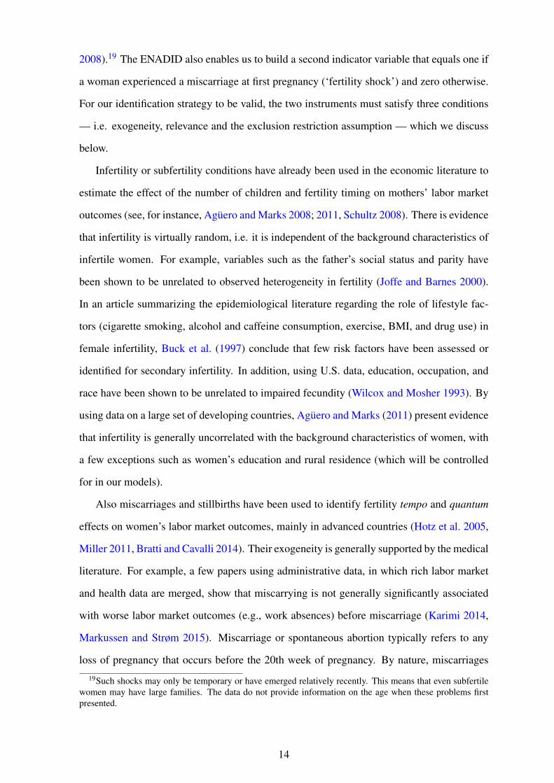
2008).19 The ENADID also enables us to build a second indicator variable that equals one if

a woman experienced a miscarriage at first pregnancy (‘fertility shock’) and zero otherwise.

For our identification strategy to be valid, the two instruments must satisfy three conditions

— i.e. exogeneity, relevance and the exclusion restriction assumption — which we discuss

below.

Infertility or subfertility conditions have already been used in the economic literature to

estimate the effect of the number of children and fertility timing on mothers’ labor market

outcomes (see, for instance, Agüero and Marks 2008; 2011, Schultz 2008). There is evidence

that infertility is virtually random, i.e. it is independent of the background characteristics of

infertile women. For example, variables such as the father’s social status and parity have

been shown to be unrelated to observed heterogeneity in fertility (Joffe and Barnes 2000).

In an article summarizing the epidemiological literature regarding the role of lifestyle fac-

tors (cigarette smoking, alcohol and caffeine consumption, exercise, BMI, and drug use) in

female infertility, Buck et al. (1997) conclude that few risk factors have been assessed or

identified for secondary infertility. In addition, using U.S. data, education, occupation, and

race have been shown to be unrelated to impaired fecundity (Wilcox and Mosher 1993). By

using data on a large set of developing countries, Agüero and Marks (2011) present evidence

that infertility is generally uncorrelated with the background characteristics of women, with

a few exceptions such as women’s education and rural residence (which will be controlled

for in our models).

Also miscarriages and stillbirths have been used to identify fertility tempo and quantum

effects on women’s labor market outcomes, mainly in advanced countries (Hotz et al. 2005,

Miller 2011, Bratti and Cavalli 2014). Their exogeneity is generally supported by the medical

literature. For example, a few papers using administrative data, in which rich labor market

and health data are merged, show that miscarrying is not generally significantly associated

with worse labor market outcomes (e.g., work absences) before miscarriage (Karimi 2014,

Markussen and Strøm 2015). Miscarriage or spontaneous abortion typically refers to any

loss of pregnancy that occurs before the 20th week of pregnancy. By nature, miscarriages

19Such shocks may only be temporary or have emerged relatively recently. This means that even subfertilewomen may have large families. The data do not provide information on the age when these problems firstpresented.

14

should have a negative effect on total fertility, and in our context on sibship size.20 Only

two etiological factors for miscarriage are recognized by different authors in the obstetrics

literature, i.e. uterine malformations and the presence of balanced chromosomal rearrange-

ments in parents (Plouffe et al. 1992). The latter though, are unlikely to be correlated with

women’s attitudes towards offspring’s migration. The number of miscarriages and stillbirths

generally increases with the number of pregnancies, which depend in turn on desired fertil-

ity, and this could potentially generate a spurious positive correlation between the number

of miscarriages and observed fertility. For this reason, we consider only miscarriages that

occurred at the first pregnancy (Miller 2011). There is a potential issue of measurement error

with this instrument, since women may be unaware of miscarriages or, especially the case

with older women, may fail to recall them. Misreporting may generally affect the power

of the instrument, but we do not expect any specific pattern of correlation between it and

parents’ attitudes towards child out-migration conditional on the observables (including a

quadratic in the mother’s age). Finally, as it was formulated in the ENADID, the question

does not distinguish between voluntary and involuntary abortions. Thus, it may be the case

that some of the reported abortions were actually voluntary, even though induced abortion

was illegal and Mexico had the strictest anti-abortion legislation in Latin America during the

period under consideration.21

For our instruments to be valid, in addition to exogeneity, they have to satisfy the ex-

clusion restriction assumption, i.e. fertility and infertility shocks must have an impact on

children’s migration only through sibship size. For this reason, in the child migration equa-

tion we control for many variables that may act as a confounding factor and those that may

be affected by the shocks while having a direct effect on children’s migration. Among

20According to Bongaarts and Potter (1983) overall spontaneous loss rates are about 20 percent of recognizedpregnancies (i.e. one out of five). Casterline (1989) stresses that in most societies pregnancy losses produce areduction of fertility of 5-10% from the levels expected in the absence of miscarriages and stillbirths.

21 For women who voluntary have an abortion, the instrument would be endogenous. However, there isno evident sign in our data that a relevant share of the recorded abortions could be voluntary. For instance,Catholic women in our sample do not tend to abort significantly less than other women (this check can be doneonly for the 1997 wave, which includes information on religion): for the first group the incidence of abortionis 4.6 percent and for the second group is 4.8 percent. In case the instrument is substantially contaminatedby voluntary abortions, we would expect IV estimates to be biased in the same direction as OLS. Indeed,omitting subscripts and in the models without controls, if we define as M = β0+β1S+v the migration equation,where M and S are child migration status and sibship size, respectively, and S = γ0 + γ1Z + u the sibshipsize equation (the first stage) and Z the instrument (abortion), β1,OLS = β1 +Cov(S,v)/Var(S) while β1,IV =β1 +Cov(Z,v)/Cov(Z,S), where Cov(Z,S)< 0 and sign(Cov(S,v)) =−sign(Cov(Z,v)). In case, for instance,unobserved mother’s total desired fertility is positively correlated with children’s migration and a substantialshare of abortions are voluntary, both OLS and IV will be similarly upward biased.

15

these variables, we include the mother’s age, age at first pregnancy, education, chronic ill-

ness/disability, marital status and the husband’s characteristics (age, education and absence).

Table 2 reports the incidence of infertility and miscarriage shocks in our (individual and

household-level) estimation samples. Data clearly show a monotonic negative association

between infertility and sibship size. For instance, while 13.4 percent and 11.4 percent of

women with family sizes equal to one or two (i.e. sibship sizes zero or one), respectively,

have experienced an infertility condition, the incidence falls to 3.5 percent for women with

seven children or more. A negative relationship also emerges between miscarriage and sib-

ship size, although it is not monotonic. In Figures 4 and 5 we report a preliminary visual

representation of the relevance of our instruments (more compelling evidence is provided

by the first-stage of the IVs reported in Section 5). In particular, we use ENADID data to

plot the average number of live births by women’s age and infertility shock and miscarriage

status. 22 Figure 4 shows that women who ever experienced an infertility condition generally

have a lower number of children, and those differences in fertility tend to increase with age.

Similarly, Figure 5 displays a negative association between miscarriage at first pregnancy

and the total number of live births. Both figures suggest that our instruments are relevant.

They also suggest that, although the shocks we consider have a negative impact on family

size, overall Mexican women were able to achieve a generally high fertility rate by the end

of their fecund life span. This is due to the fact that exogenous infertility shocks, as defined

in this and related papers, clearly affect the number of children a woman can have but they

also may be temporary (i.e. secondary infertility) or treatable so that fertility may eventually

be restored.

[Table 2 about here]

[Figure 4 and 5 about here]22Older women belong to earlier birth cohorts, whose fertility is likely to be higher. For women below 45

years of age, instead, fertility may not be completed.

16

5 Results

5.1 Birth order effects

We start by estimating the impact of birth order on individual migration, as specified in

equation (1), controlling for family fixed effects. The within-family estimator sweeps out

all parental- and family-level heterogeneity, including completed family size. Moreover,

family fixed effects account for omitted family-specific unobservable factors simultaneously

affecting fertility and child migration. The first column of Table 3 reports estimates with a

linear specification of birth order on the full sample, whereas in column (2) we allow for a

more flexible specification by adding birth-order-specific dichotomous indicators. Regres-

sions control for individual age and gender plus child cohort dummies (one for each year

of birth).23 Indeed, child age is correlated with birth order and it is also likely to have a

(non-linear) relationship with migration (which is why we include the age quadratic term).

First, in column (1) we observe that, after controlling for family fixed effects, birth order

and individual characteristics, females are significantly less likely to migrate than males

by 3.6 percentage points (p.p.). Moreover, the birth order point estimate is negative and

statistically significant. The effect starts to be economically significant from children of birth

order 3, who are about 2.1 p.p. less likely to migrate than firstborns (column 2). Although

this appears to be a small effect in absolute value, it represents an approximately 40 percent

decrease in migration at the sample average (5.2 percent migration rate). The coefficients for

the following birth orders are larger in absolute value and peak for birth orders 9 and 10 or

more (-16.6 and -20 p.p. respectively).

In columns (3) and (4) we estimate the same regressions as above by adding interaction

effects between birth order and gender to the models.24 We observe a negative birth order

gradient for boys (the coefficients on the third and higher parities are negative and signifi-

cant), which is consistent with the average results above. The interactions of being female

with birth order dummies are not statistically significant, suggesting that the birth-order gra-

23By including child age and cohort dummies, with household fixed effects, we are also de facto controllingfor birth spacing between siblings.

24As our two-step procedure relies on family fixed effects, when estimating separate regressions by genderonly families with at least two sons and at least two daughters can be included in the estimates for males andfemales, respectively. In order to avoid such a sample selection, we rather adopt a pooled estimation includinginteraction effects with gender.

17

dient in child migration is not statistically different between boys and girls. Yet, the latter

holds for all parities but for firstborns: in column (4) the female main effect shows that fe-

male firstborns are significantly less likely to migrate than male firstborns. Overall, these

estimates suggest that the chances of migration are not equally distributed across children

within the same family. Low-parity children are in general more likely to migrate and this

may be explained by the fact that, if migration is also a household-level investment strategy,

the family will have more time to reap the benefits of migration. Yet, from our fidings a

firstborn daughter is significantly less likely to migrate than a firstborn son by 3 p.p., which

means a reduction in the probability of migration of roughly 60 percent at the sample aver-

age migration rate. We further explore these gendered effects in light of potential parental

preferences below in Section 5.4.

[Table 3 about here]

5.2 Sibship size effect: WLS and 2SLS results at the individual-level

In this Section, we turn to the estimation of the sibship size effects. By applying the two-

step procedure described above, we start by reporting WLS estimates as a benchmark model,

where the dependent variable is ‘netted migration’ (see Section 4.1).25 The number of sib-

lings is tallied as the number of currently living biological brothers and sisters of each child.26

The first column of Table 4 reports WLS results for a linear specification including sibship

size. The highly significant coefficient implies that, on average and after controlling for birth

order effects, adding one sibling is associated with a 1.1 p.p. higher likelihood of migrating

for young adults (+17 percent at the sample mean). The same effect holds once we include

individual level controls, namely child gender, age, age squared and years of birth indica-

tors (column 2). When we allow for differential effects by child gender (column 3), the

significant negative coefficient for the interaction term indicates that the female likelihood to

migrate increases less due to sibship size than for males. Specifically, one extra sibling raises

25The inverse of the standard errors of ‘netted migration’ are used as weights.26Those currently deceased are excluded from our definition of siblings. This is so because of two reasons:

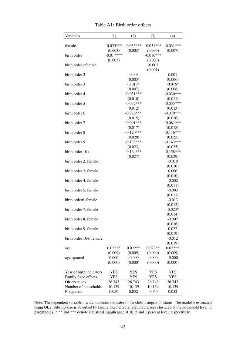
(i) 70 per cent of deceased children in our sample died before the first year of life, 90 per cent of them beforethe second one; (ii) the focus of our analysis is not on young children so that we need to take into accountsiblings who actually ‘had enough time’ to both receive and compete over household resources, so that canexclude infant deaths. In Appendix, we report robustness checks related to concerns about the endogeneity ofour definition of sibship size and birth order based on ever-born children, i.e. currently alive or deceased.

18

the migration probability more for sons than for daughters by 0.8 p.p. In columns (4) to (7),

we run the same regressions above while adding further parental, household and aggregate-

level controls in order to account for potential confounding factors of the relationship be-

tween family size and offspring’s migration. Specifically, in column (3) and (4) we include

parental covariates, which may predict completed fertility and affect child migration, namely

mother’s years of birth indicators, age at first pregnancy, chronic illness, single status (i.e.

widow, divorced, single de facto), father’s decade of birth indicators, mothers’ and father’s

(quadratic) age and years of schooling.27 In column (5) and (6) we further add municipal-

ity fixed effects that, conditional on family size, control for rural vs. urban residence along

with many other local factors related to different cultural or economic conditions, which

may have an effect on fertility and migration (e.g., employment rates, migration intensity,

access to contraception, social services etc). Overall, the sibiship size effect is essentially

unchanged when we control for all of the aforementioned factors, and the same holds for the

differential effect by gender.

[Table 4 about here]

Yet, as noted in the methodological section, the coefficients on sibship size reported in

Table 4 are still likely to be biased, even when including a rich set of demographic and eco-

nomic controls. This is so as fertility may be endogenous with respect to child out-migration.

Thus we employ an IV approach and exploit the arguably exogenous fertility variation gener-

ated by episodes of infertility and miscarriage. Since these events can vary the actual family

size from the desired one, we use infertility shocks and miscarriage at first pregnancy to

identify the effect of sibship size on child out-migration. In Table 5 we present two-stage

least squares (2SLS) estimates using a linear version of our ‘saturated’ specification (with

controls) and the two-step methodology, as outlined above, to estimate equation (2). In col-

umn (1) we instrument sibship size with an indicator variable for infertility shocks taking

value one if the woman declares she never used or she stopped using contraception because

of infertility. In column (2), instead, we report results using a woman’s experience of mis-

carriage on her first pregnancy as an instrument. Eventually, in column (3) we present results27We are de facto also controlling for mother’s age at delivery, which is a linear combination of child’s age

and mother’s age. As far as parental controls are concerned, we have more missing information for fathers thanit is the case for mothers. As to keep the sample size constant, we further include a dummy variable for missinginformation of fathers.

19

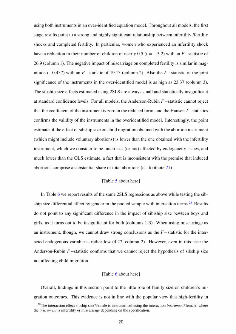
using both instruments in an over-identified equation model. Throughout all models, the first

stage results point to a strong and highly significant relationship between infertility /fertility

shocks and completed fertility. In particular, women who experienced an infertility shock

have a reduction in their number of children of nearly 0.5 (t =−5.2) with an F−statistic of

26.9 (column 1). The negative impact of miscarriage on completed fertility is similar in mag-

nitude (−0.437) with an F−statistic of 19.13 (column 2). Also the F−statistic of the joint

significance of the instruments in the over-identified model is as high as 23.37 (column 3).

The sibship size effects estimated using 2SLS are always small and statistically insignificant

at standard confidence levels. For all models, the Anderson-Rubin F−statistic cannot reject

that the coefficient of the instrument is zero in the reduced form, and the Hansen J−statistics

confirms the validity of the instruments in the overidentified model. Interestingly, the point

estimate of the effect of sibship size on child migration obtained with the abortion instrument

(which might include voluntary abortions) is lower than the one obtained with the infertility

instrument, which we consider to be much less (or not) affected by endogeneity issues, and

much lower than the OLS estimate, a fact that is inconsistent with the premise that induced

abortions comprise a substantial share of total abortions (cf. footnote 21).

[Table 5 about here]

In Table 6 we report results of the same 2SLS regressions as above while testing the sib-

ship size differential effect by gender in the pooled sample with interaction terms.28 Results

do not point to any significant difference in the impact of sibiship size bewteen boys and

girls, as it turns out to be insignificant for both (columns 1-3). When using miscarriage as

an instrument, though, we cannot draw strong conclusions as the F−statistic for the inter-

acted endogenous variable is rather low (4.27, column 2). However, even in this case the

Anderson-Rubin F−statistic confirms that we cannot reject the hypothesis of sibship size

not affecting child migration.

[Table 6 about here]

Overall, findings in this section point to the little role of family size on children’s mi-

gration outcomes. This evidence is not in line with the popular view that high-fertility in28The interaction effect sibship size*female is instrumented using the interaction instrument*female, where

the instrument is infertility or miscarriage depending on the specification.

20

developing countries is a major cause of international emigration: according to our estimates

this correlation is driven by unobservable variables which make some families more prone

to both have more children and send some of them abroad.

5.3 Robustness checks: Household-level estimates

In this section, we estimate the migration equation while using the household instead of the

individual as the unit of analysis.29 In so doing we are able to check the robustness of our

baseline family size effect to changing the estimation sample and strategy. Indeed, the two-

step procedure reported above is based on household fixed effects and therefore can only

be applied to households with more than one child in the full sample. By contrast, while

focusing on the total number of migrants in the household as a function of total fertility, we

do not need to control for birth order effects and we can use a standard IV procedure. As a

consequence, household-level regressions allow us to include also one-child households in

the sample.30 Thus, we estimate a specification as follows:

m j = γ0 + γ1n j + γ2W j + v j (3)

where the dependent variable is the number of children in the age range 15-25 who ever

migrated in household j and the independent variable of interest is n j, i.e. the total number

of children in household j. The coefficient γ1 captures the increase in the number of migrants

associated with a unitary increase in the number of children. Like in the child-level estimates,

W j includes family background characteristics such as the mother’s and the father’s age, age

squared, and years of completed education, mother’s age at first pregnancy, an indicator for

the father not being in the household and municipality fixed effects; v j is an household-level

error term. This specification is estimated both with OLS and with IVs (namely two-stage

least squares).

[Table 7 about here]

Results are reported in Table 7. Column (1) shows that a unit increase in the number of

29More precisely, our unit of analysis is the biological family.30Thus, in these estimates we also exploit individuals who do not have siblings, and look at whether they are

more (less) likely to migrate than individuals with siblings.

21

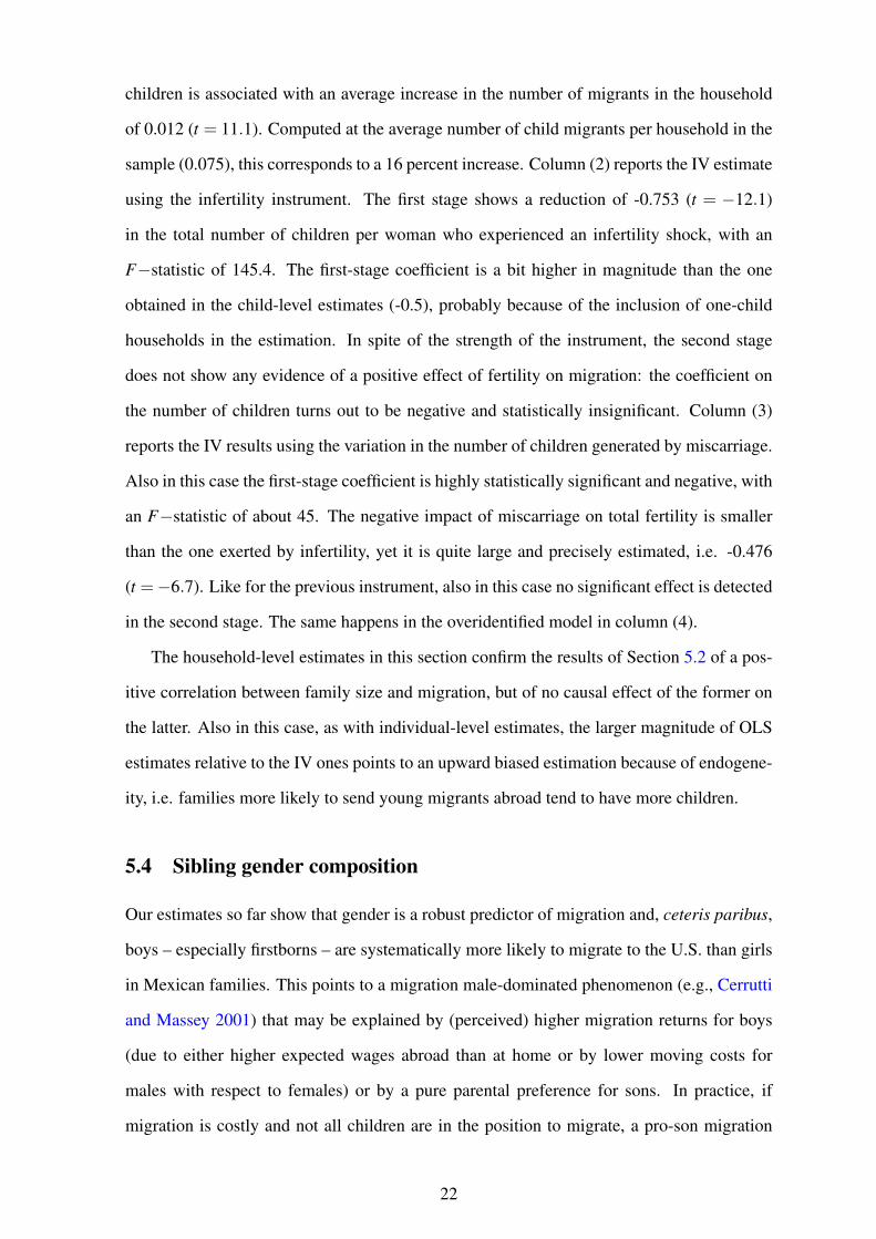
children is associated with an average increase in the number of migrants in the household

of 0.012 (t = 11.1). Computed at the average number of child migrants per household in the

sample (0.075), this corresponds to a 16 percent increase. Column (2) reports the IV estimate

using the infertility instrument. The first stage shows a reduction of -0.753 (t = −12.1)

in the total number of children per woman who experienced an infertility shock, with an

F−statistic of 145.4. The first-stage coefficient is a bit higher in magnitude than the one

obtained in the child-level estimates (-0.5), probably because of the inclusion of one-child

households in the estimation. In spite of the strength of the instrument, the second stage

does not show any evidence of a positive effect of fertility on migration: the coefficient on

the number of children turns out to be negative and statistically insignificant. Column (3)

reports the IV results using the variation in the number of children generated by miscarriage.

Also in this case the first-stage coefficient is highly statistically significant and negative, with

an F−statistic of about 45. The negative impact of miscarriage on total fertility is smaller

than the one exerted by infertility, yet it is quite large and precisely estimated, i.e. -0.476

(t =−6.7). Like for the previous instrument, also in this case no significant effect is detected

in the second stage. The same happens in the overidentified model in column (4).

The household-level estimates in this section confirm the results of Section 5.2 of a pos-

itive correlation between family size and migration, but of no causal effect of the former on

the latter. Also in this case, as with individual-level estimates, the larger magnitude of OLS

estimates relative to the IV ones points to an upward biased estimation because of endogene-

ity, i.e. families more likely to send young migrants abroad tend to have more children.

5.4 Sibling gender composition

Our estimates so far show that gender is a robust predictor of migration and, ceteris paribus,

boys – especially firstborns – are systematically more likely to migrate to the U.S. than girls

in Mexican families. This points to a migration male-dominated phenomenon (e.g., Cerrutti

and Massey 2001) that may be explained by (perceived) higher migration returns for boys

(due to either higher expected wages abroad than at home or by lower moving costs for

males with respect to females) or by a pure parental preference for sons. In practice, if

migration is costly and not all children are in the position to migrate, a pro-son migration

22

bias may lead to a situation in which children compete for household resources in order to

migrate and such ‘rivalry’ can yield gains to having relatively more sisters than brothers

(Garg and Morduch 1998). Thus, in order to explore the scope of sibling rivalry by gender,

we test how sibling composition influences child migration investment by running two sets

of regressions as reported in Table 8. First, we estimate migration equations on the full

sample of children as a function of the number of their older brothers, while controlling for

both family and birth order fixed effects (i.e., conditioning on the number of both siblings

and older siblings), child gender, (quadratic) age and cohort dummies. Results in column (1)

show that, ceteris paribus, having an older brother (sister) instead of an older sister (brother)

decreases (increases) the migration probability by 1.4 p.p. (t = 3.6). This result points

to a significant role of the gender and age composition of siblings in children’s migration

outcomes, which does not differ significantly by the child’s gender (column 2).

[Table 8 about here]

Yet, we further exploit the gendered migration pattern and the fact that siblings are likely

to migrate in order of birth (with higher parities being less likely to migrate, as shown by our

former estimates in section 5.1) to test the hypothesis of parental son preference. We do so

by including a control for having a next-born brother in the family fixed effects regressions

on the pooled-sample (with and without interactive effects), as above. If a child has at least

one younger sibling, the gender of his/her next-born sibling is random and a comparison

of children with next-born brothers with children with next-born sisters, while controlling

for older siblings composition, can identify the effect of the sibling’s gender.31 Results in

columns (3) and (4) in Table 8 show that, conditional on older siblings’ composition, having

a next-born brother does not play any role for sons, but reduces the likelihood to migrate for

girls with respect to boys by 1.2 p.p. (t =−2). This result suggests that when parents decide

the level of investment in their children’s out-migration, the siblings’ composition by gender

and age matters. More specifically, from our results it seems that a daughter with a next-born

brother may be less likely to migrate than a girl with a next-born sister. In other words, when

parents face the decision whether to send a daughter abroad, they seem to prefer to invest

31A similar empirical strategy has been used in Vogl (2013) to study sibling rivalry over arranged marriagesin South Asia.

23

in the migration of her next-born brother. These results are in line with other evidence from

developing countries that, when there are high returns to investing in the human capital of

children but resources are limited, children may become rivals (even in the absence of any

explicit strategic behavior on the part of any family member) and typically girls turn out to

be disadvantaged when they compete with boys (Dunn and Plomin 1990, Kristin and Anne

1994, Morduch 2000). Indeed, our findings are suggestive that children, especially girls,

with relatively more brothers than sisters are less likely to migrate abroad than their peers.

These results, combined with the birth order effects reported above, are consistent with

the argument that a low-parity Mexican boy may be more valuable to send as a migrant

abroad than a girl. Indeed, labor market returns for Mexican boys in the U.S. were relatively

higher in the 1990s (e.g., in the farm sector). In addition, the opportunity cost of sending

girls abroad may be higher because they usually take care of chores and family duties at

home or are in charge of being close to parents in their elderly age. Hence, social norms

or practices combined with market returns on the migration investment may explain the

pro-male biased pattern of mass Mexico-U.S. migration and document, similarly to other

developing contexts, that young females tend to have less access to human capital investment

and enhancing economic opportunities than it is the case for males.

6 Conclusions

In this paper we provide novel and rigorous evidence on the extent to which international

labor mobility is affected by the demographic characteristics of the migrant’s household.

Migration is largely a youth phenomenon that occurs in households that never dispatch all of

their children to work abroad. With capital market imperfections and high migration costs,

the ‘resource dilution’ hypothesis predicts that a larger sibship size will decrease the chances

of offspring’s migration. Yet, in relatively poor contexts, parents are likely to depend on

their grown children for the provision of care and income, and high rates of migration can

significantly contribute to the living arrangements of elderly parents.

We use a rich household-survey dataset on teenagers and young adults to examine the

causal effects of sibship size, birth order and sibling composition on migration outcomes in

Mexico. Mexican migration, mainly to the U.S., is an enduring flow that account for one third

24

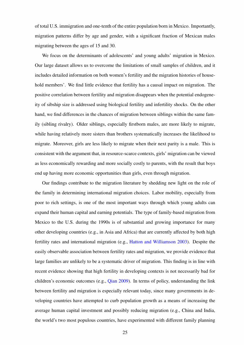
of total U.S. immigration and one-tenth of the entire population born in Mexico. Importantly,

migration patterns differ by age and gender, with a significant fraction of Mexican males

migrating between the ages of 15 and 30.

We focus on the determinants of adolescents’ and young adults’ migration in Mexico.

Our large dataset allows us to overcome the limitations of small samples of children, and it

includes detailed information on both women’s fertility and the migration histories of house-

hold members’. We find little evidence that fertility has a causal impact on migration. The

positive correlation between fertility and migration disappears when the potential endogene-

ity of sibship size is addressed using biological fertility and infertility shocks. On the other

hand, we find differences in the chances of migration between siblings within the same fam-

ily (sibling rivalry). Older siblings, especially firstborn males, are more likely to migrate,

while having relatively more sisters than brothers systematically increases the likelihood to

migrate. Moreover, girls are less likely to migrate when their next parity is a male. This is

consistent with the argument that, in resource-scarce contexts, girls’ migration can be viewed

as less economically rewarding and more socially costly to parents, with the result that boys

end up having more economic opportunities than girls, even through migration.

Our findings contribute to the migration literature by shedding new light on the role of

the family in determining international migration choices. Labor mobility, especially from

poor to rich settings, is one of the most important ways through which young adults can

expand their human capital and earning potentials. The type of family-based migration from

Mexico to the U.S. during the 1990s is of substantial and growing importance for many

other developing countries (e.g., in Asia and Africa) that are currently affected by both high

fertility rates and international migration (e.g., Hatton and Williamson 2003). Despite the

easily observable association between fertility rates and migration, we provide evidence that

large families are unlikely to be a systematic driver of migration. This finding is in line with

recent evidence showing that high fertility in developing contexts is not necessarily bad for

children’s economic outcomes (e.g., Qian 2009). In terms of policy, understanding the link

between fertility and migration is especially relevant today, since many governments in de-

veloping countries have attempted to curb population growth as a means of increasing the

average human capital investment and possibly reducing migration (e.g., China and India,

the world’s two most populous countries, have experimented with different family planning

25

policies to control family size). Yet, although our empirical findings do not point to a causal

link between fertility and migration, they hint to the fact that parental investment in off-

spring’s migration may matter for lifetime fertility choices. This is so as in a context of poor

resources and weak institutional safety nets, children may be a key social security valve for

parents such that high migration opportunities to rich countries increase the value of having

children. Hence, effective safety and welfare measures (such as old age pensions) or even

the development of credit and insurance markets may lead to a reduction in both migration

and fertility, and also perhaps a lesser gender gap.

26

ReferencesAgüero, J. M. and M. S. Marks (2008). Motherhood and female labor force participation:

Evidence from infertility shocks. American Economic Review 98(2), 500–504.

Agüero, J. M. and M. S. Marks (2011). Motherhood and female labor supply in the de-veloping world: Evidence from infertility shocks. Journal of Human Resources 46(4),800–826.

Amuedo-Dorantes, C. and S. Pozo (2011). Remittances and income smoothing. The Ameri-can Economic Review, Papers and Proceedings 102(3), 582–587.

Angrist, J., V. Lavy, and A. Schlosser (2010). Multiple experiments for the causal linkbetween the quantity and quality of children. Journal of Labor Economics 28(4), 773–824.

Antman, F. (2012). Elderly care and intrafamily resource allocation when children migrate.Journal of Human Resources 47(2), 331–63.

Ashenfelter, O. (2012). Comparing real wage rates: Presidential address. American Eco-nomic Review 102(2), 617–42.

Bagger, J., J. A. Birchenall, H. Mansour, and S. Urzúa (2013). Education, Birth Order, andFamily Size. NBER Working Papers 19111, National Bureau of Economic Research, Inc.

Becker, G. S. (1960). An economic analysis of fertility. In G. S. Becker (Ed.), Demo-graphic and Economic Change in Developed Countries,. Princeton, NJ: Princeton Univer-sity Press.

Becker, G. S. and H. Lewis (1973). On the interaction between the quantity and quality ofchildren. Journal of Political Economy 81(2), S279–S288.

Becker, G. S. and N. Tomes (1976). Child endowments and the quantity and quality ofchildren. Journal of Political Economy 84(4), S143–62.

Billari, F. C. and V. Galasso (2014, April). Fertility decisions and pension reforms. Evidencefrom natural experiments in Italy. IdEP Economic Papers 1403, USI Università dellaSvizzera italiana.

Black, S. E., P. J. Devereux, and K. G. Salvanes (2005). The more the merrier? The effect offamily size and birth order on children’s education. The Quarterly Journal of Economics,669–700.

Bongaarts, J. and R. Potter (1983). Fertility, Biology, and Behavior: An Analysis of theProximate Determinants. New York: Academy Press.

Borjas, G. J. and L. F. Katz (2005). The evolution of the Mexican-born workforce in theUnited States. NBER Working Papers 11281, National Bureau of Economic Research,Inc.

Bratti, M. and L. Cavalli (2014). Delayed first birth and new mothers’ labor market out-comes: Evidence from biological fertility shocks. European Journal of Population 30(1),35–63.

27

Brezis, E. S. and R. D. S. Ferreira (2014). Endogenous fertility with a sibship size effect.Working Papers of BETA 2014-03, Bureau d’Economie Théorique et Appliquée, UDS,Strasbourg.

Buck, G. M., L. E. Sever, R. E. Batt, and P. Mendola (1997). Life-style factors and femaleinfertility. Epidemiology 8(4), 435–41.

Cabrera, G. (1994). Demographic dynamics and development: The role of population policyin mexico. Population and Development Review 20, 105–120.

Casterline, J. (1989). Collecting data on pregnancy loss: A review of evidence from theWorld Fertility Survey. Studies in Family Planning 20(2), 81–95.

Cerrutti, M. and D. Massey (2001). On the auspices of female migration from Mexico to theUnited States. Demography 38(2), 187–200.

Chen, J. J. (2006). Migration and imperfect monitoring: Implications for intra-householdallocation. American Economic Review 96(2), 227–231.

Chen, K.-P., S.-H. Chiang, and S. F. Leung (2003). Migration, family, and risk diversifica-tion. Journal of Labor Economics 21(2), 323–352.

Cigno, A. (1993). Intergenerational transfers without altruism: Family, market and state.European Journal of Political Economy 9(4), 505–518.

Clemens, M. (2011). Economics and emigration: Trillion-dollar bills on the sidewalk? Jour-nal of Economic Perspectives 25(3), 83–106.

Clemens, M., C. E. Montenegro, and L. Pritchett (2010). The place premium: Wage dif-ferences for identical workers across the us border. Working papers, University of Chile,Department of Economics.

Clemens, M. A., a. Özden, and H. Rapoport (2014). Migration and development research ismoving far beyond remittances. World Development 64(C), 121–124.

Duflo, E. and A. Banerjee (2011). Poor Economics: A Radical Rethinking of the Way toFight Global Poverty. PublicAffairs.

Dunn, J. and R. Plomin (1990). Separate Lives: Why Siblings are so Different. Basic Books,New York.

Dustmann, C. and A. Glitz (2011). Migration and education. In E. Hanushek, S. Machin,and L. Woessmann (Eds.), Handbook of the Economics of Education, Volume 4, ChapterChapter 4, pp. 327–439. Amsterdam: Elsevier.

Fitzsimons, E. and B. Malde (2014, January). Empirically probing the quantity-qualitymodel. Journal of Population Economics 27(1), 33–68.

Garg, A. and J. Morduch (1998). Sibling rivalry and the gender gap: Evidence from childhealth outcomes in Ghana. Journal of Population Economics 11(4), 471–493.

Gábos, A., R. Gál, and G. Kézdi (2009). The effects of child-related benefits and pensionson fertility. Population Studies 63(3), 215–231.

Ghatak, S., P. L. and S. W. Price (1996). Migration theories and evidence: An assessment.Journal of Economic Surveys 10(2), 159–197.

28

Gibson, J. and D. McKenzie (2012). The economic consequences of ‘brain drain’of thebest and brightest: Microeconomic evidence from five countries. The Economic Jour-nal 122(560), 339–375.

Giles, J. and R. Mu (2007). Elderly parent health and the migration decisions of adult chil-dren: Evidence from rural China. Demography 44(2), 265–288.

Hanson, G. (2004). Illegal migration from Mexico to the United States. Journal of EconomicLiterature Vol. 44(4), 869–924.

Hanson, G. H. and C. McIntosh (2010). The Great Mexican migration. The Review ofEconomics and Statistics 92(4), 798810.

Hanushek, E. A. (1992). The trade-off between child quantity and quality. Journal of Politi-cal Economy 100(1), 84–117.

Hatton, T. J. and J. G. Williamson (1998). The Age of Mass Migration: Causes and EconomicImpact. New York: Oxford University Press.

Hatton, T. J. and J. G. Williamson (2003). Demographic and Economic Pressure on Emigra-tion out of Africa. Scandinavian Journal of Economics 105(3), 465–486.

Hotz, V. J., S. W. McElroy, and S. G. Sanders (2005). Teenage childbearing and its lifecycle consequences: Exploiting a natural experiment. Journal of Human Resources 40(3),683–715.

Jayachandran, S. and R. Pande (2015). Why are indian children so short? NBER WorkingPapers 21036, National Bureau of Economic Research, Inc..

Jensen, R. and N. Miller (2011). Keepin’ ’em down on the farm: Old age security andstrategic underinvestment in children. mimeo UCLA (4).

Joffe, M. and I. Barnes (2000). Do parental factors affect male and female fertility? Epi-demiology 11(6), 700–705.

Karimi, A. (2014, August). Effects of the timing of births on women’s earnings – Evidencefrom a natural experiment. Working Paper Series 2014:17, IFAU – Institute for Evaluationof Labour Market and Education Policy.

Kennan, J. and J. R. Walker (2011). The Effect of Expected Income on Individual MigrationDecisions. Econometrica 79(1), 211–251.

Kristin, B. and C. Anne (1994). The effect of sibling sex composition on women’s educationand earnings. The Quarterly Journal of Economics 109(3).

Lewis, J. B. and D. A. Linzer (2005). Estimating regression models in which the dependentvariable is based on estimates. Political Analysis 13(4), 345–364.

Lucas, R. E. B. and O. Stark (1985). Motivations to remit: Evidence from Botswana. Journalof Political Economy 93(5), 901–18.

Markussen, S. and M. Strøm (2015). The effects of motherhood. Technical report, MEMO-RANDUM No 19/2015, Department of Economics, University of Oslo.

Martin, P. L. (1993). Trade and Migration: NAFTA and Agriculture. Washington: Institutefor International Economics.

29

Mckenzie, D. and H. Rapoport (2007). Network effects and the dynamics of migration andinequality: Theory and evidence from Mexico. Journal of Development Economics 84(1),1–24.

Miller, A. (2011). The effect of motherhood timing on career path. Journal of PopulationEconomics 24(3), 1071–1100.

Miller, G. and K. S. Babiarz (2014). Family planning program effects. NBER Working PaperNo. 20586.

Morduch, J. (2000). Sibling rivarly in Africa. American Economic Review 90 (2), 405–409.

Mourard, E. (2015). The impact of migration on the family left behind: Estimation in pres-ence of intra-household selection of the migrants. Paris School of Economics. Mimeo..

Nugent, J. (1985). The old-age security motive for fertility. Population and DevelopmentReview 11(1), 75–97.

Ozden, C. and M. Schiff (2006). International Migration, Remittances, and the Brain Drain.Washington, DC: The World Bank and Palgrave McMillan.

Pande, R. (2003). Selective gender differences in childhood nutrition and immunization inrural India: The role of siblings. Demography 40(3), 395–418.

Parish, W. L. and R. J. Willis (1993). Daughters, education, and family budgets Taiwanexperiences. Journal of Human Resources 28(4), 863–898.

Platteau, J. (1991). Traditional systems of social security and hunger insurance: Pastachievements and modern challenges. Clarendon Press, Oxford.

Plouffe, L. J., T. S. White E. W., C. Sweet, L. Layman, G. Whitman, and P. McDonough(1992). Etiologic factors of recurrent abortion and subsequent reproductive performanceof couples: Have we made any progress in the past 10 years? American Journal ofObstetrics and Gynecology 167(2), 313–321.

Qian, N. (2009). Quantity-Quality and the One Child Policy:The Only-Child Disadvantagein School Enrollment in Rural China. NBER Working Papers 14973, National Bureau ofEconomic Research, Inc.

Rapoport, H. and F. Docquier (2006, 00). The Economics of Migrants’ Remittances, Vol-ume 1 of Handbook on the Economics of Giving, Reciprocity and Altruism, Chapter 17,pp. 1135–1198. Elsevier.

Ratha, D., S. Mohapatra, and E. Scheja (2011). Impact of migration on economic and socialdevelopment: A review of evidence and emerging issues. Policy Research Working PaperSeries 5558, The World Bank 61(3), 380–89.

Ray, D. (1998). Development Economics. New York: Princeton, NJ: Princeton UniversityPress.

Rosenzweig, M. (2007). Education and migration: A global perspective. Yale University.Mimeo.

Rosenzweig, M. R. (1988). Risk, implicit contracts and the family in rural areas of low-income countries. Economic Journal 98(393), 1148–70.

30

Rosenzweig, M. R. and O. Stark (1989). Consumption smoothing, migration, and marriage:Evidence from rural India. Journal of Political Economy 97(4), 905–26.

Rosenzweig, M. R. and K. I. Wolpin (1980). Testing the quantity-quality fertility model:The use of twins as a natural experiment. Econometrica 48(1), 227–240.

Schultz, T. (2008). Population policies, fertility, women’s human capital, and child quality.Volume 4, Chapter 52, pp. 3249–3303. Amsterdam: Elsevier.

Schultz, T. P. (1990). Testing the neoclassical model of family labor supply and fertility.Journal of Human Resources 25(4), 599–634.

Schultz, T. W. (1972). Human capital: Policy issues and research opportunities. In EconomicResearch: Retrospect and Prospect Vol 6: Human Resources, pp. 1–84. UMI.

Sjaastad, L. (1962). The costs and returns of human migration. Journal of Political Econ-omy 70(5), 80–93.

Stark, O. (1981). The asset demand for children during agricultural moderninzation. Popu-lation and Development Review 4(3), 671–675.

Stark, O. (1991). The migration of labour. Basil Blackwell, Cambridge.

Stark, O. and D. E. Bloom (1985). The New Economics of Labor Migration. AmericanEconomic Review 75(2), 173–78.

Stöhr, T. (2015, July). Siblings interaction in migration decisions: Who provides for theelderly left behind? Journal of Population Economics 28(3), 593–629.

Suits, D. B. (1984). Dummy variables: Mechanics v. interpretation. The Review of Eco-nomics and Statistics 66(1), 177–80.

Thomas, D. (1990). Intra-household resource allocation: An inferential approach. Journalof Human Resources 25(4), 635–664.

UN (2013). World youth report. Technical report, United Nations.

UNDESA (2011). The age and sex of migrants. Technical report, United Nation, Departmentof Economics and Social Affairs, Population Division.

Vogl, T. S. (2013). Marriage institutions and sibling competition: Evidence from south Asia.The Quarterly Journal of Economics 128(3), 1017–1072.

Wilcox, L. S. and W. D. Mosher (1993). Use of infertility services in the United States.Obstetrics & Gynecology 82(1), 122–127.

Williamson, J. (1990). Coping with City Growth during the British Industrial Revolution.Cambridge, MA: Harvard University Press.

Yang, D. (2008). International migration, remittances and household investment: Evidencefrom Philippine migrants’ exchange rate shocks. Economic Journal 118(528), 591–630.

Zuniga Herrera, E. (2008). Population policy in Mexico and its relationship to development.presented at Contribution of Population Policy to the Achievement of the Internation-ally Development Goals including the MDGs. Panel discussion, New York, 15 December2008.

31

Figure 1: Mexican individual (non-tied) migration by age and gender

0.0

2.0

4.0

6.0

8.1

.12

5 20 35 50Age at migration

Male Female

Source: Our computations on ENADID, 1992 and 1997.

Figure 2: Individual migration rate by family size

0.0

5.1

.15

2 3 4 5 6 7 8 9 10 11Family size

Male Female

Source: Our computations on ENADID, 1992 and 1997.

32

Figure 3: Ratio of migrant children by family size

0.1

.2.3

.4.5

.6

2 3 4 5 6 7 8 9 10Family size

Share of migrant children Distribution of family size

Source: Our computations on ENADID, 1992 and 1997 (subsample of households with migrants).

Figure 4: Average number of children by women’s infertility shock status

12

34

56

No.

of l

ive

birth

s

30 35 40 45 50 55Women's age

Infertile Fertile

Note. Source: ENADID, 1992 and 1997. The figure reports the average number of live births by women’sinfertility shock status and age. Regression lines are super-imposed to the cross-plot.

33

Figure 5: Average number of children by women’s miscarriage at first pregnancy

23

45

6N

o. o

f liv

e bi

rths

30 35 40 45 50 55Women's age

Miscarriage No Miscarriage

Note. Source: ENADID, 1992 and 1997. The figure reports the average number of live births by miscarriageat first pregnancy and age. Regression lines are super-imposed to the cross-plot.

34

Table 1: Sample characteristics by migration status

Non-migrants Migrants p−values(A) (B) (A)-(B)

Individual-level characteristicsAge 18.878 20.982 0.000Female 0.458 0.250 0.000N. of siblings 5.071 5.869 0.000Birth order 1 0.181 0.192 0.300Birth order 2 0.231 0.225 0.555Birth order 3 0.178 0.178 0.978Birth order 4 0.137 0.154 0.077Birth order 5 0.102 0.102 0.993Birth order 6 0.071 0.073 0.781Birth order 7 0.046 0.041 0.343Birth order 8 0.028 0.021 0.100Birth order 9 0.014 0.009 0.121Birth order 10+ 0.011 0.006 0.107Household-level characteristicsMother’s age 44.612 46.171 0.000Mother’s age at first pregnancy 20.030 19.699 0.182Mother’s years of schooling 4.091 3.452 0.010Mother chronic illness 0.023 0.008 0.131Single mother 0.185 0.188 0.896Mother’s labor income 600.403 862.540 0.037Father’s age 48.799 52.207 0.000Father’s years of schooling 4.931 3.789 0.059

Note. Source: ENADID, 1992 and 1997. The estimation sample includes individuals aged 15–25 whosemothers are not using contraceptive methods. The sample comprises 1,394 migrants and 25,349 non-migrantindividuals.

Table 2: Incidence of fertility and infertility shocks by sibship size

Individual sample Household sampleIncidence of shock (%) Incidence of shock (%)

sibship size % infertility miscarriage sibship size % infertility miscarriage

0 3.69 13.37 5.051 4.59 11.56 6.03 1 9.84 11.43 6.802 12.16 8.33 5.38 2 16.88 7.48 5.203 14.20 5.45 4.06 3 15.96 5.16 4.024 14.68 5.12 4.05 4 13.66 4.30 3.865 13.54 4.00 5.55 5 11.20 3.73 4.71

6+ 40.82 3.94 3.68 6+ 28.76 3.51 3.44100.00 100.00

Note. The table reports the incidence of fertility and infertility shocks in the estimation samples used in theindividual-level (see Section 5.2) and the household-level analysis (see Section 5.3 ), respectively.

35

Table 3: Birth order effects

Variables (1) (2) (3) (4)

female -0.036*** -0.035*** -0.032*** -0.031***(0.003) (0.003) (0.006) (0.007)

birth order -0.019*** -0.019***(0.003) (0.003)

birth order × female -0.001(0.001)

birth order 2 -0.002 0.002(0.005) (0.006)

birth order 3 -0.021*** -0.023***(0.007) (0.008)

birth order 4 -0.038*** -0.034***(0.010) (0.011)

birth order 5 -0.068*** -0.070***(0.013) (0.014)

birth order 6 -0.086*** -0.077***(0.016) (0.017)

birth order 7 -0.112*** -0.103***(0.019) (0.020)

birth order 8 -0.136*** -0.140***(0.022) (0.023)

birth order 9 -0.161*** -0.166***(0.026) (0.028)

birth order 10+ -0.199*** -0.188***(0.030) (0.033)

birth order 2, female -0.011(0.009)

birth order 3, female 0.005(0.010)

birth order 4, female -0.010(0.010)

birth order 5, female 0.006(0.011)

birth order 6, female -0.018(0.012)

birth order 7, female -0.017(0.015)

birth order 8, female 0.010(0.018)

birth order 9, female 0.012(0.024)

birth order 10+, female -0.022(0.027)

age 0.020** 0.021** 0.020** 0.021**(0.009) (0.009) (0.009) (0.009)

age squared 0.000 0.000 0.000 0.000(0.000) (0.000) (0.000) (0.000)

Year of birth indicators YES YES YES YESFamily fixed effects YES YES YES YESObservations 26,743 26,743 26,743 26,743R-squared 0.050 0.052 0.050 0.053

Note. The dependent variable is a dichotomous indicator of the child’s migration status. The model is estimatedusing OLS. Sibship size is absorbed by family fixed effects. Standard errors clustered at the household level inparentheses. *,** and *** denote statistical significance at 10, 5 and 1 percent level, respectively.

36

Table 4: Sibship size effect: WLS estimates

Variables (1) (2) (3) (4) (5) (6) (7)

N. siblings 0.011*** 0.011*** 0.014*** 0.010*** 0.013*** 0.010*** 0.013***(0.001) (0.001) (0.001) (0.001) (0.001) (0.001) (0.001)

N. siblings × female(a) -0.008*** -0.007*** -0.006***(0.001) (0.001) (0.001)

female -0.038*** -0.036*** -0.033*** -0.031*** -0.033*** -0.031***(0.003) (0.006) (0.003) (0.006) (0.003) (0.003)

Individual’s controls NO YES YES YES YES YES YESMother’s controls NO NO NO YES YES YES YESFather’s controls NO NO NO YES YES YES YESMunicipality indicators NO NO NO NO NO YES YESObservations 26,743 26,743 26,743 26,743 26,743 26,743 26,743R-squared 0.013 0.054 0.055 0.177 0.178 0.202 0.203

Note. The dependent variable is netted migration (see Section 4). The model is estimated using Weighted LeastSquares (weights are the inverse of the standard errors of netted migration). Individual’s controls include yearof birth indicators, age, age squared; mother’s controls include year of birth indicators, age and age squared,age at first pregnancy, years of schooling, indicators for mother’s chronic illness and being single; father’scontrols include decade of birth indicators, age and age squared, years of schooling. Standard errors clusteredat the household level in parentheses. (a) The number of siblings is demeaned before taking the interaction.*,** and *** denote statistical significance at 10, 5 and 1 percent level, respectively.

37

Table 5: Sibliship size effect: 2SLS estimates

Variables (1) (2) (3)

Second stageN. siblings 0.004 -0.018 -0.005

(0.014) (0.023) (0.012)female -0.033*** -0.033*** -0.033***

(0.003) (0.003) (0.003)

IV: infertility miscarriage overidentifiedAnderson-Rubin F−statistic 0.073 0.686 0.389

[0.787] [0.407] [0.678]Hansen J−statistic 0.737

[0.391]

First stage — N. siblingsinfertility -0.494*** -0.491***

(0.095) (0.095)miscarriage -0.437*** -0.433***

(0.10) (0.10)Angrist-Pischke F−statistic instrument(s) 26.90 19.13 23.37Individual’s controls YES YES YESMother’s controls YES YES YESFather’s controls YES YES YESMunicipality indicators YES YES YESObservations 26,743 26,743 26,743

Note. The dependent variable is netted migration (see Section 4). Observations are weighted by the inverse ofthe standard error of netted migration. Individual’s controls include year of birth indicators, age, age squared;mother’s controls include year of birth indicators, age and age squared, age at first pregnancy, years of school-ing, indicators for mother’s chronic illness and being single; father’s controls include decade of birth indica-tors, age and age squared, years of schooling. Standard errors clustered at the household level in parentheses.P−values are reported in brackets. *,** and *** denote statistical significance at 10, 5 and 1 percent level,respectively.

38

Table 6: Child gender and sibship size effect: 2SLS estimates

Variables (1) (2) (3)

Second stageN. siblings 0.005 -0.065 -0.007

(0.016) (0.048) (0.015)N. siblings × female(a) -0.005 0.112 0.005

(0.013) (0.079) (0.013)female -0.032*** -0.064*** -0.034***

(0.004) (0.022) (0.005)

IV: infertility miscarriage overidentifiedAnderson-Rubin F−statistic 0.074 2.210 1.150

[0.928] [0.110] [0.331]Hansen J−statistic 4.399

[0.111]

First stage — N. siblingsinfertility -0.567*** -0.564***

(0.109) (0.108)infertility × female 0.168 0.169

(0.115) (0.115)miscarriage -0.453*** -0.450***

(0.117) (0.117)miscarriage × female 0.037 0.038

(0.106) (0.105)Angrist-Pischke F−statistic instrument(s) 28.62 11.98 15.68

First stage — N. siblings × femaleinfertility 0.125*** 0.125***

(0.038) (0.038)infertility × female -0.694*** -0.691***

(0.131) (0.131)miscarriage -0.067 -0.068

(0.044) (0.043)miscarriage × female -0.261** -0.254*

(0.131) (0.130)Angrist-Pischke F−statistic instrument(s) 26.93 4.27 13.83Individual’s controls YES YES YESMother’s controls YES YES YESFather’s controls YES YES YESMunicipality indicators YES YES YESObservations 26,743 26,743 26,743

Note. The dependent variable is netted migration (see Section 4). Observations are weighted by the inverse ofthe standard error of netted migration. Individual’s controls include year of birth indicators, age, age squared;mother’s controls include year of birth indicators, age and age squared, age at first pregnancy, years of school-ing, indicators for mother’s chronic illness and being single; father’s controls include decade of birth indica-tors, age and age squared, years of schooling. Standard errors clustered at the household level in parentheses.P−values are reported in brackets. (a) The number of siblings is demeaned before taking the interaction. *,**and *** denote statistical significance at 10, 5 and 1 percent level, respectively.

39

Table 7: Family size effect: Household-level estimates

(1) (2) (3) (4)Variables OLS 2SLS 2SLS 2SLS

Second stageN. children 0.012*** 0.001 -0.016 -0.003

(0.001) (0.010) (0.020) (0.009)

IV: — infertility miscarriage overidentifiedAnderson-Rubin F−statistic 0.008 0.640 0.324

[0.928] [0.424] [0.723]Hansen J−statistic 0.580

[0.446]

First stage — N. childreninfertility - 0.753*** -0.750***

(0.062 ) (0.062)miscarriage -0.476*** -0.469***

(0.071) (0.071)Angrist-Pischke F−statistic instrument(s) 145.42 44.95 96.17Mother’s controls YES YES YES YESFather’s controls YES YES YES YESMunicipality indicators YES YES YES YESObservations 18,217 18,217 18,217 18,217

Note. The dependent variable is a dummy for the child’s migration status. Mother’s controls include yearof birth indicators, age and age squared, age at first pregnancy, years of schooling, indicators for mother’schronic illness and being single; father’s controls include decade of birth indicators, age and age squared, yearsof schooling. P−values are reported in brackets. *,** and *** denote statistical significance at 10, 5 and 1percent level, respectively.

Table 8: Siblings’ composition effect: OLS estimates

Variables (1) (2) (3) (4)

N. older brothers -0.014*** -0.014*** -0.017*** -0.016***(0.004) (0.004) (0.004) (0.005)

female -0.028*** -0.026*** -0.022*** -0.016***(0.003) (0.005) (0.005) (0.006)

N. older brothers × female -0.002 -0.002 -0.003(0.002) (0.002) (0.002)

Next brother -0.005 0.001(0.004) (0.004)

Next brother × female -0.012**(0.006)

Age, age squared YES YES YES YESBirth order fixed effects YES YES YES YESYear of birth indicators YES YES YES YESFamily fixed effects YES YES YES YESObservations 26,743 26,743 26,743 26,743Number of hid 10,139 10,139 10,139 10,139R-squared 0.053 0.053 0.053 0.053

Note. The dependent variable is a dichotomous indicator of the child’s migration status. The model is estimatedusing OLS. Sibship size is absorbed by family fixed effects. Standard errors clustered at the household level inparentheses. *,** and *** denote statistical significance at 10, 5 and 1 percent level, respectively.

40

A Appendix: Sibship size including deceased children

41

Table A1: Birth order effects

Variables (1) (2) (3) (4)

female -0.035*** -0.035*** -0.031*** -0.031***(0.003) (0.003) (0.005) (0.007)

birth order -0.017*** -0.016***(0.003) (0.003)

birth order×female -0.001(0.001)

birth order 2 -0.003 0.001(0.005) (0.006)

birth order 3 -0.013* -0.016*(0.007) (0.008)

birth order 4 -0.031*** -0.030***(0.010) (0.011)

birth order 5 -0.057*** -0.055***(0.012) (0.013)

birth order 6 -0.076*** -0.070***(0.015) (0.016)

birth order 7 -0.091*** -0.081***(0.017) (0.018)

birth order 8 -0.120*** -0.116***(0.020) (0.022)

birth order 9 -0.133*** -0.143***(0.023) (0.025)

birth order 10+ -0.164*** -0.158***(0.027) (0.029)

birth order 2, female -0.010(0.010)

birth order 3, female 0.006(0.010)

birth order 4, female -0.002(0.011)

birth order 5, female -0.003(0.011)

birth order6, female -0.013(0.012)

birth order 7, female -0.023*(0.014)

birth order 8, female -0.007(0.016)

birth order 9, female 0.022(0.019)

birth order 10+, female -0.012(0.019)

age 0.022** 0.022** 0.022** 0.022**(0.009) (0.009) (0.009) (0.009)

age squared 0.000 -0.000 0.000 -0.000(0.000) (0.000) (0.000) (0.000)

Year of birth indicators YES YES YES YESFamily fixed effects YES YES YES YESObservations 26,743 26,743 26,743 26,743Number of households 10,139 10,139 10,139 10,139R-squared 0.050 0.052 0.050 0.052

Note. The dependent variable is a dichotomous indicator of the child’s migration status. The model is estimatedusing OLS. Sibship size is absorbed by family fixed effects. Standard errors clustered at the household level inparentheses. *,** and *** denote statistical significance at 10, 5 and 1 percent level, respectively.

42

Table A2: Sibship size effect: WLS estimates

Variables (1) (2))

N. siblings 0.010*** 0.013***(0.001) (0.001)

N. siblings × female(a) -0.007***(0.001)

female -0.032*** -0.030***(0.003) (0.003)

Individual’s controls YES YESMother’s controls YES YESFather’s controls YES YESMunicipality indicators YESWeighted YES YESObservations 26,743 26,743R-squared 0.204 0.206

Note. The dependent variable is netted migration (see Section 4). The model is estimated using WeightedLeast Squares (the weights are the inverse of the standard errors of netted migration). Individual’s controlsinclude year of birth indicators, age, age squared; mother’s controls include year of birth indicators, age andage squared, age at first pregnancy, years of schooling, indicators for mother’s chronic illness and being single;father’s controls include decade of birth indicators, age and age squared, years of schooling. Standard errorsclustered at the household level in parentheses. (a) The number of siblings is demeaned before taking theinteraction. *,** and *** denote statistical significance at 10, 5 and 1 percent level, respectively.

43

Table A3: Sibship size effect: 2SLS estimates

Variables (1) (2) (3)

Second stageN. siblings 0.002 -0.015 -0.005

(0.014) (0.024) (0.013)female -0.032*** -0.033*** -0.032***

(0.003) (0.003) (0.003)

IV: infertility miscarriage overidentifiedAnderson-Rubin F−statistic 0.0229 0.433 0.232

[0.880] [0.510] [0.793]Hansen J−statistic 0.419

[0.517]

First stage — N. siblingsinfertility -0.475*** -0.472***

(0.095) (0.095)miscarriage -0.411*** -0.407***

(0.10) (0.10)Angrist-Pischke F−statistic instrument(s) 25.01 17.78 21.70Individual’s controls YES YES YESMother’s controls YES YES YESFather’s controls YES YES YESMunicipality indicators YES YES YESObservations 26,743 26,743 26,743

Note. The dependent variable is netted migration (see Section 4). Observations are weighted by the inverse ofthe standard error of netted migration. Individual’s controls include year of birth indicators, age, age squared;mother’s controls include year of birth indicators, age and age squared, age at first pregnancy, years of school-ing, indicators for mother’s chronic illness and being single; father’s controls include decade of birth indica-tors, age and age squared, years of schooling. Standard errors clustered at the household level in parentheses.P−values are reported in brackets. *,** and *** denote statistical significance at 10, 5 and 1 percent level,respectively.

44

Table A4: Child gender and sibliship size effect: 2SLS estimates

Variables (1) (2) (3)

Second stageN. siblings 0.002 -0.065 -0.006

(0.016) (0.057) (0.015)N. siblings × female(a) -0.001 0.105 0.007

(0.013) (0.084) (0.013)female -0.032*** -0.059*** -0.034***

(0.004) (0.022) (0.004)

IV: infertility miscarriage overidentifiedAnderson-Rubin F−statistic 0.0115 1.577 0.797

[0.989] [0.207] [0.527]Hansen J−statistic 2.925

[0.232]

First stage — N. siblingsinfertility -0.557*** -0.555***

(0.107) (0.107)infertility × female 0.168 0.190*

(0.115) (0.114)miscarriage -0.390*** -0.387***

(0.113) (0.113)miscarriage × female 0.046 -0.046

(0.106) (0.102)Angrist-Pischke F−statistic instrument(s) 31.59 5.74 19.49

First stage — N. siblings × femaleinfertility 0.135*** 0.136***

(0.039) (0.038)infertility × female -0.689*** -0.686***

(0.134) (0.134)miscarriage -0.066 -0.068

(0.044) (0.044)miscarriage × female -0.287** -0.280**

(0.131) (0.130)Angrist-Pischke F−statistic instrument(s) 40.51 4.55 17.22Individual’s controls YES YES YESMother’s controls YES YES YESFather’s controls YES YES YESMunicipality indicators YES YES YESObservations 26,743 26,743 26,743

Note. The dependent variable is netted migration (see Section 4). Observations are weighted by the inverse ofthe standard error of netted migration. Individual’s controls include year of birth indicators, age, age squared;mother’s controls include year of birth indicators, age and age squared, age at first pregnancy, years of school-ing, indicators for mother’s chronic illness and being single; father’s controls include decade of birth indica-tors, age and age squared, years of schooling. Standard errors clustered at the household level in parentheses.P−values are reported in brackets. (a) The number of siblings is demeaned before taking the interaction. *,**and *** denote statistical significance at 10, 5 and 1 percent level, respectively.

45