28
Fast 3-D Interconnect Capacitance Extraction and Related Numerical Techniques Wenjian Yu EDA Lab, Dept. Computer Science & Technology, Tsinghua University Nov. 22, 2004
| Date post: | 22-Dec-2015 |
| Category: |
Documents |
| View: | 217 times |
| Download: | 1 times |

Fast 3-D Interconnect Capacitance Extraction and Related Numerical Techniques
Wenjian Yu
EDA Lab, Dept. Computer Science & Technology, Tsinghua University
Nov. 22, 2004
2
Outline
Background 3-D capacitance extraction with direct BEM Fast capacitance extraction with QMM
acceleration and other numerical techniques Numerical results Conclusion
3
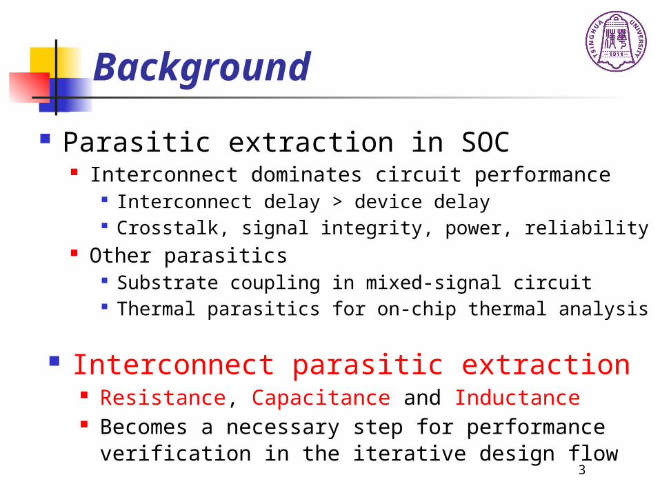
Background
Parasitic extraction in SOC Interconnect dominates circuit performance
Interconnect delay > device delay Crosstalk, signal integrity, power, reliability
Other parasitics Substrate coupling in mixed-signal circuit Thermal parasitics for on-chip thermal analysis
Interconnect parasitic extraction Resistance, Capacitance and Inductance Becomes a necessary step for performance
verification in the iterative design flow
4
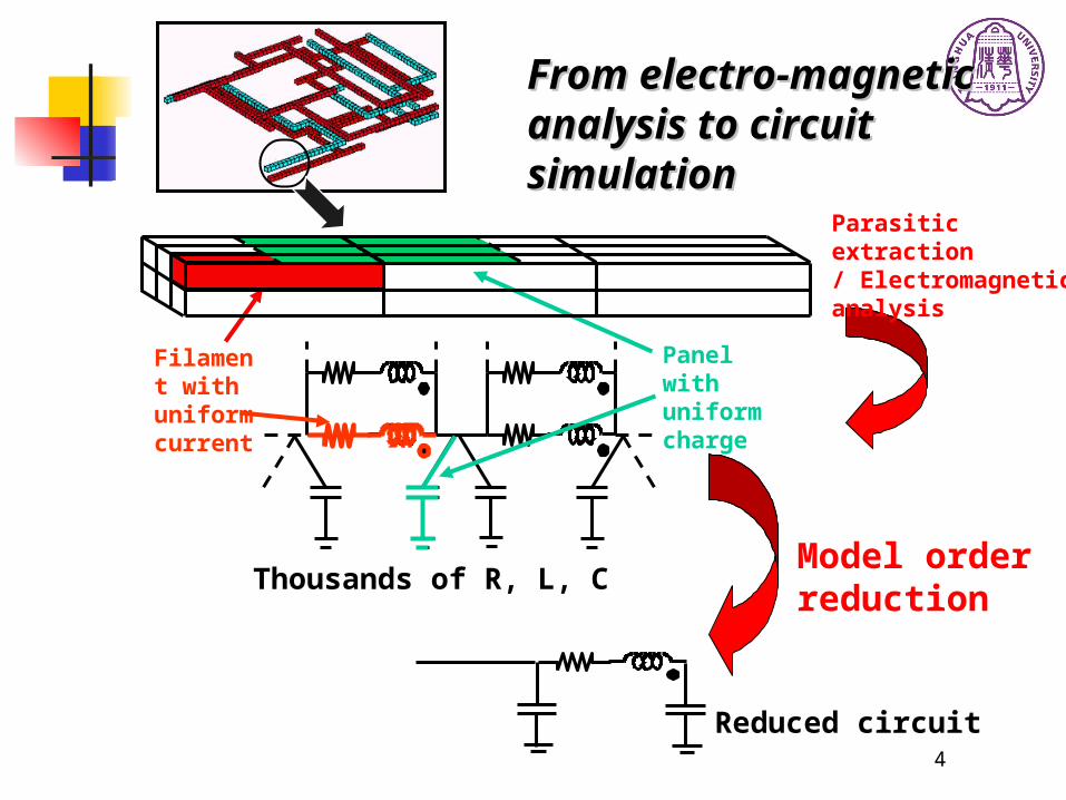
From electro-magnetic From electro-magnetic analysis to circuit simulationanalysis to circuit simulation
Parasitic extraction/ Electromagnetic analysis
Thousands of R, L, C
Filament with uniform current
Panel with uniform charge
Model orderreduction
Reduced circuit

5
VLSI capacitance extraction
Capacitance extraction For m conductors solve m
potential problems for the conductor surface charges
Electric potential u fulfill:
Capacitance is function of wire shape, environment, distance to substrate, distance to surrounding wires
Challenges: high accuracy (3-D method), high speed, suitable for complex process
1V
0V
1 2
34
CC11ii= -Q= -Qii ((ii1)1)2 2 2
2 2 2( ) 0
u u uu
x y z

6
VLSI capacitance extraction
3-D methods for capacitance extraction Finite difference /
Finite element Sparse matrix, but with
large number of unknowns
Boundary integral formulation (BEM) Fewer unknowns, more accurate, handle complex geom
etry Two kinds: indirect BEM makes dense matrix direct BEM has localization property Both BEM’s need Krylov subspace iterative solver
and fast algorithms (multipole acceleration, hierarchical, precorrected FFT, SVD-based, quasi-multiple medium, …)

7
Direct BEM for Cap. Extraction
Physical equations Laplace equation within each subregion Finite domain model Bias voltages set on conductors
conductorconductor
uq
2
1
u is electrical potential
q is normal electrical field intensity on boundary

8
Direct BEM for Cap. Extraction
Direct boundary element method Green’s Identity
Freespace Green’s function as weighting function The Laplace equation is transformed into the BIE:
ii
dquduquc ssss** s is a collocation point
More details: C. A. Brebbia, The Boundary Element Method for Engineers, London: Pentech Press, 1978
2 2( ) ( )v u
u v v u d u v d
n n
*su is freespace Green’s function, o
r the fundamental solution of Laplace equation

9
Direct BEM for Cap. Extraction
Discretize domain boundary• Partition quadrilateral elements with
constant interpolation
• Non-uniform element partition
• Integrals (of kernel 1/r and 1/r3) in discretized BIE:
N
jjs
N
jjsss
jj
qduudquc1
*
1
* )()(
• Singular integration
• Non-singular integration• Dynamic Gauss point selection
• Semi-analytical approach improves
computational speed and accuracy for near singular integration
P3(x3,y2,z2) Y
Z X O
P4(x4,y2,z2)
P2(x2,y1,z1) P1(x1,y1,z1)
ss
ttjj

10
Direct BEM for Cap. Extraction
Write the discretized BIEs as:iiii qGuH , (i=1, …, M)
fAx • Non-symmetric large-scale matrix A
• Use GMRES to solve the equation
• Charge on conductor is the sum of q
Compatibility equations Compatibility equations along the interfacealong the interface
ba
bbbaaauu
uu nn
For problem involving multiple regions, matrix For problem involving multiple regions, matrix AA exhibits sparsity! exhibits sparsity!

11
Fast algorithms - QMM
Quasi-multiple medium method In each BIE, all variables are within same dielectric region; this l
eads to sparsity when combining equations for multiple regions
u q
substrate
①
②
③
3-dielectric structure
v11 v22 v33u12 q21 u23 q32
s11
s12
s21
s22
s23
s32
s33
Population of matrix A
Make fictitious cutting on the normal structure, to enlarge the matrix sparsity in the direct BEM simulation.
With iterative equation solver, sparsity brings actual benefit.
QMM !

12
EnvironmentConductors
Master Conductor
x
y
z
A 3-D multi-dielectric case within finite domain, applied 32 QMM cutting
Fast algorithms - QMM
QMM-based capacitance extraction Make QMM cutting Then, the new structure with many
subregions is solved with the BEM
Time analysis while the iteration number
dose not change a lot
Z: number of non-zeros in the final coefficient matrix At Z
Confirmed in our later experiments

13
Fast algorithms - QMM
Select optimal cutting pair Empirical formula, or manually specifying Automatic selection, make total computation achieve
highest speed; make use of the linear relationship between computational time and the parameter Z
FlowchartDetermine the set S containing the
candidates of cutting numbers
Calculate the Z-value for a cuttingnumber in the set S
Select the optimal cutting numberaccording to the Z-values
Cutting pair: (3, 2)
with minimal Z-val

14
Fast algorithms - QMM
Calculate the Z-value Two types of boundary element
Nuemann: one u variable / element Dirichlet: one q variable / element Interface: both u and q variable / element
)2)(( iiiiiii babaVNZ So,
N
jjs
N
jjsss
jj
qduudquc1
*
1
* )()( The discretized BIE:
Q
iiZZ
1
ai( Type 1)
( Type 2) bi
Heuristic rules for set S -- candidates of (m, n) Relatively small size for the sake of saving time Moderate value range of m (along X-axis) and n (along Y-axis) Range is relevant to the dimensions along X/Y-axis
Need not construct the actual geometry & boundary mesh !

15
Example of matrix population
12 subregions af12 subregions after applying 2ter applying 22 2 QMMQMM
Too many subregions produce complexity of equation organizing and storing
Bad scheme makes non-zero entries dispersed, and worsens the efficiency of matrix-vector multiplication in iterative solution
We order unknowns and collocation points correspondingly; suitable for multi-region problems with arbitrary topology
Fast algorithms - Equ. organ.
Three Three stratified stratified mediummedium
v11 v22 v33u12 q21 u23 q32
s11
s12
s21
s22
s23
s32
s33
16
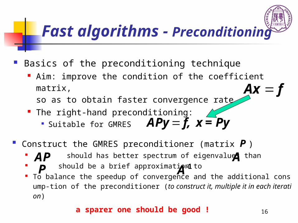
Fast algorithms - Preconditioning
Basics of the preconditioning technique Aim: improve the condition of the coefficient matrix,
so as to obtain faster convergence rate The right-hand preconditioning:
Suitable for GMRES
fAx
APy f, x = Py
a sparer one should be good !
Construct the GMRES preconditioner (matrix P ) should has better spectrum of eigenvalues than should be a brief approximation to To balance the speedup of convergence and the additional consump-t
ion of the preconditioner (to construct it, multiple it in each iteration)
AP AP -1A
17
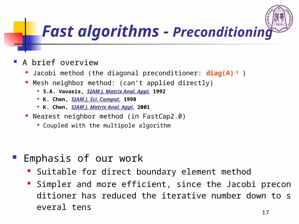
Fast algorithms - Preconditioning
A brief overview Jacobi method (the diagonal preconditioner: diag(A)-1 ) Mesh neighbor method: (can’t applied directly)
S.A. Vavasis, SIAM J. Matrix Anal. Appl. 1992 K. Chen, SIAM J. Sci. Comput. 1998 K. Chen, SIAM J. Matrix Anal. Appl. 2001
Nearest neighbor method (in FastCap2.0) Coupled with the multipole algorithm
Emphasis of our work Suitable for direct boundary element method Simpler and more efficient, since the Jacobi preconditioner has reduc
ed the iterative number down to several tens

18
T
ip =010
A
Reduced equation
Fast algorithms - Preconditioning
Principle of the MN method The neighbor variables of variable i:
Solve the reduced equation , fill back to ith row of P
, 1, ..., T T Ti i i N PA I A P I A p e
1 2{ , , ... , } {1, 2, ... , }nL l l l N T
i iA p e
A
Var. i
l1 l2 l 3
P i
l1 l2 l 3
Solve, and fill P

19
Fast algorithms - Preconditioning
Extended Jacobi preconditioner Singular integral is importance Singular integrals from interface elements
are not all at the main diagonal Except for row corresponding to interface
element, solve a 22 reduced equation to involve all singular integrals
MN (n) preconditioner n is the number of neighbor elements Scan the ith row, use the absolute value as measure of neighborhood When n=1, 2, performs well
v11 v22 v33u12 q21 u23 q32
s11
s12
s21
s22
s23
s32
s33
30% or more time reduction, compared with using the Jacobi preconditioner, for more than 100 structures

20
Fast algorithms - nearly linear
Efficient organization and solution technique ensure near linear relationship between the total computing time and non-zero matrix entries (Z-values)
For two cases from actual layout:
0
0.5
1
1.5
2
2.5
3
3.5
4
0 200 400 600Z -value (103)
Com
putin
g tim
e (s
)
0
5
10
15
20
25
30
35
0 2000 4000 6000Z -value (103)
Com
putin
g tim
e (s
)
m: 2~9, n: 2~6 m: 2~7, n: 2~10

21
Numerical results (1)
Experiment environment SUN UltraSparc II processors (248 MHz) Programs
Our QMM-BEM solver: QBEM FastCap 2.0: FastCap(1), FastCap(2) Raphael RC3 (3-D finite difference solver)
Test examples kk crossovers in five
layered dielectrics (k=2 to 5)
Finite domain
C1 is calculated for comparison The 2x2 case
x
z
1 2
34
22
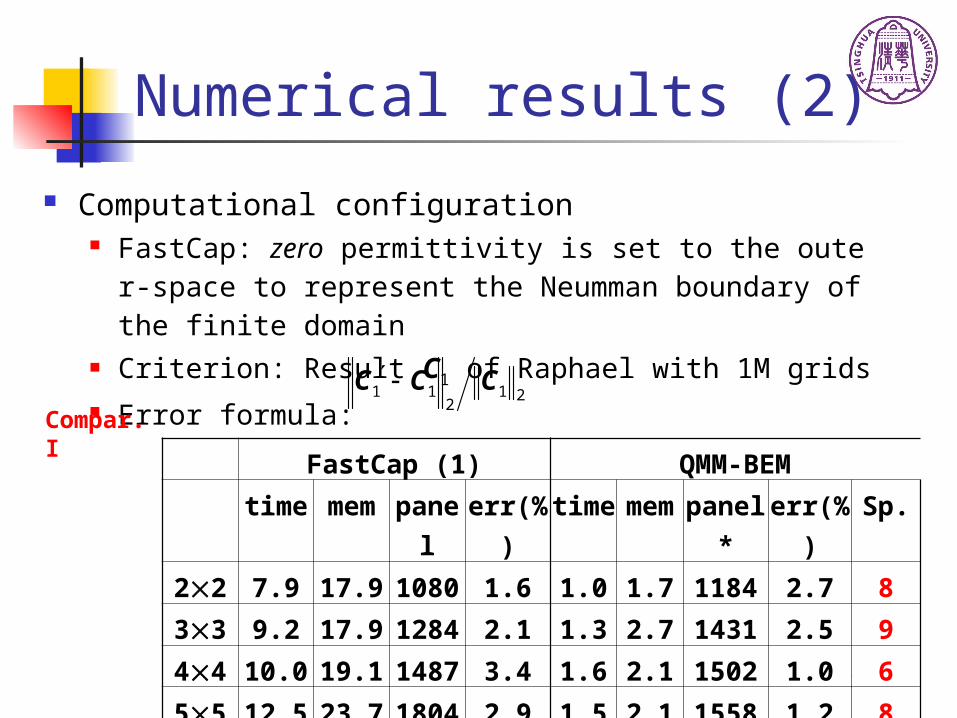
Numerical results (2)
Computational configuration FastCap: zero permittivity is set to the outer-space to repre
sent the Neumman boundary of the finite domain Criterion: Result C1 of Raphael with 1M grids Error formula: 1 1 1 2
2
C C C
FastCap (1) QMM-BEM
time mem panel err(%) time mem panel* err(%) Sp.
22 7.9 17.9 1080 1.6 1.0 1.7 1184 2.7 8
33 9.2 17.9 1284 2.1 1.3 2.7 1431 2.5 9
44 10.0 19.1 1487 3.4 1.6 2.1 1502 1.0 6
55 12.5 23.7 1804 2.9 1.5 2.1 1558 1.2 8
Compar. I

23
Numerical results (3)
Raphael (0.25M) QMM-BEM
time mem panel err(%) time mem panel* err(%) Sp.
22 78.8 47 - 0.3 1.0 1.7 1184 2.7 79
33 67.1 45 - 0.4 1.3 2.7 1431 2.5 52
44 88.9 48 - 0.5 1.6 2.1 1502 1.0 56
55 81.9 48 - 0.8 1.5 2.1 1558 1.2 55
Compar. III
FastCap (2) QMM-BEM
time mem panel err(%) time mem panel* err(%) Sp.
22 11.5 26.4 1080 2.1 1.0 1.7 1184 2.7 12
33 15.1 28.4 1284 2.3 1.3 2.7 1431 2.5 12
44 17.5 30.7 1487 2.6 1.6 2.1 1502 1.0 11
55 24.3 38.5 1804 3.0 1.5 2.1 1558 1.2 16
Compar. II

24
Numerical results (4)
Our QMM-BEM solver Panel* don’t count the panels on interfaces between fictitious media The optimal QMM cutting pairs are (4, 4), (5, 5), (3, 3), (3, 3) respectiv
ely ; the EJ preconditioner is uesed
Comparison IV. Computational details for the 44 crossover problem
panel Ele_N Var_N Z-val Iter. mem Tgen(s) Tsol(s) Time
QBEM 1502 1896 2435 0.24M 11 2.1 1.02 0.29 1.6
FastCap(1) 1487 1487 1487 - 13 19.1 6.9 2.9 10.0
FastCap(2) 1487 1487 1487 - 9 30.7 13.4 4.0 17.5
Tgen: time of generating the linear systemTsol: time of solving the linear system

25
Discussion
FastCap QBEM
Formulation Single-layer potential formula Direct boundary integral equation
System matrix Dense Dense for single-region, otherwise sparse
Matrix degree N, the number of panels A little larger than N
Acceleration Multipole method: less than N2 operations in each matrix-ve
ctor product
QMM method -- maximize the matrix spar
sity: much less than N2 operations in each
matrix-vector product
Other cost Cube partition and multipole e
xpansion are expensive
Efficient organizing and storing of sparse
matrix make matrix-vector product easy
Resemblance: boundary discretization stop criterion of 10-2 in GMRES solution similar preconditioning almost the same iteration number
Contrast

26
Conclusion
Numerical techniques in the QMM-BEM solver Analytical / Semi-analytical integration Quasi-multiple medium acceleration (cutting pair selection) Equation organization of discretized direct BEM Preconditioning on the GMRES solver Achieve about 10x speed-up to FastCap
Related work Use the blocked Gauss method for capacitance extraction with
multiple master conductors Handle problem with floating dummies in area filling Apply the direct BEM to the substrate resistance extraction

27
For more information
Wenjian Yu, Zeyi Wang and Jiangchun Gu, “Fast capacitance extraction of a
ctual 3-D VLSI interconnects using quasi-multiple medium accelerated BEM,”
IEEE Trans. Microwave Theory Tech., Jan 2003 , 51(1): 109-120
Wenjian Yu and Zeyi Wang, “Enhanced QMM-BEM solver for 3-D multiple-di
electric capacitance extraction within the finite domain,” IEEE Trans. Micro
wave Theory Tech., Feb 2004, 52(2): 560-566
Wenjian Yu, Zeyi Wang and Xianlong Hong, “Preconditioned multi-zone boun
dary element analysis for fast 3D electric simulation,” Engng. Anal. Bound.
Elem., Sep 2004, 28(9): 1035-1044