Contents lists available at SciVerse ScienceDirect

Information Systems

Information Systems 38 (2013) 619–633

0306-43

http://d

n Corr

E-m

luciano

m.laros

journal homepage: www.elsevier.com/locate/infosys

Fast detection of exact clones in business processmodel repositories

Marlon Dumas a,n, Luciano Garcıa-Banuelos a, Marcello La Rosa b,c, Reina Uba a

a University of Tartu, Tartu, Estoniab Queensland University of Technology, Brisbane, Australiac NICTA Queensland Lab, Brisbane, Australia

a r t i c l e i n f o

Available online 25 July 2012

Keywords:

Process model repository

Clone detection

Indexing structure

Query

79/$ - see front matter & 2012 Elsevier Ltd. A

x.doi.org/10.1016/j.is.2012.07.002

esponding author. Tel.: þ372 7375473.

ail addresses: dumas@ut.ee, marlon.dumas@u

.garcia@ut.ee (L. Garcıa-Banuelos),

a@qut.edu.au (M. La Rosa), reinak@ut.ee (R. U

a b s t r a c t

As organizations reach higher levels of business process management maturity, they

often find themselves maintaining very large process model repositories, representing

valuable knowledge about their operations. A common practice within these reposi-

tories is to create new process models, or extend existing ones, by copying and merging

fragments from other models. We contend that if these duplicate fragments, a.k.a. exact

clones, can be identified and factored out as shared subprocesses, the repository’s

maintainability can be greatly improved. With this purpose in mind, we propose an

indexing structure to support fast detection of clones in process model repositories.

Moreover, we show how this index can be used to efficiently query a process model

repository for fragments. This index, called RPSDAG, is based on a novel combination of

a method for process model decomposition (namely the Refined Process Structure Tree),

with established graph canonization and string matching techniques. We evaluated the

RPSDAG with large process model repositories from industrial practice. The experi-

ments show that a significant number of non-trivial clones can be efficiently found in

such repositories, and that fragment queries can be handled efficiently.

& 2012 Elsevier Ltd. All rights reserved.

1. Introduction

Organizations engaged in long-term business processmanagement programs need to deal with repositories ofhundreds or even thousands of process models, with sizesranging from dozens to hundreds of elements per model[1,2]. For example, the SAP reference model contains over600 business process models, while Suncorp, a largeAustralian insurer, maintains a repository of over 3000process models [3]. Tool vendors nowadays distributereference model repositories (e.g. the IT InfrastructureLibrary—ITIL) with over a thousand process models each.Such models are used to document and to communicateinternal procedures, to guide the development of IT

ll rights reserved.

t.ee (M. Dumas),

ba).

systems, or to support business improvement projects,among other uses.

While highly valuable, such collections of processmodels raise a maintenance challenge [4]. This challengeis amplified by the fact that process models are generallymaintained and used by stakeholders with varying skills,responsibilities and goals, sometimes distributed acrossindependent organizational units. One problem thatarises as repositories grow is that of managing overlapacross models. In particular, process model repositoriestend to accumulate duplicate fragments over time, as newprocess models are created by copying and mergingfragments from other models. Experiments conductedduring this study have put into evidence a large numberof clones in three process model repositories from indus-trial practice. This situation is akin to that observed insource code repositories, where significant amounts ofduplicate code fragments – known as code clones – areaccumulated over time [5].

M. Dumas et al. / Information Systems 38 (2013) 619–633620

Cloned fragments in process models raise severalissues. Firstly, clones make individual process modelslarger than they need to be, thus affecting their compre-hensibility. Secondly, clones are modified independently,sometimes by different stakeholders, leading to unwantedinconsistencies across models. Finally, process modelclones hide potential efficiency gains. Indeed, by factoringout cloned fragments into separate subprocesses, andexposing these subprocesses as shared services, compa-nies may reap the benefits of larger resource pools.

Detecting clones by comparing process models in apairwise manner – using sub-graph isomorphism – wouldbe inefficient in the context of repositories with hundredsof process models. Accordingly, indexes are needed tospeed up the clone discovery process.

In this setting, this paper addresses the problem ofretrieving all clones in a process model repository thatcan be refactored into shared subprocesses. Specifically, thecontribution of the paper is an index structure, namely theRPSDAG, that provides operations for inserting and deletingmodels, as well as an operation for retrieving all clones in arepository that meet the following requirements:

�

All retrieved clones must be single-entry, single-exit(SESE) fragments, since subprocesses are invokedaccording to a call-and-return semantics. � All retrieved clones must be exact clones so that every

occurrence can be replaced by an invocation to a single(shared) subprocess. While identifying approximate

clones could be useful in some scenarios, approximateclones cannot be directly refactored into shared sub-processes, and thus fall outside the scope of this study.

� All retrieved clones are maximal, in the sense that each

of them has multiple non-identical enclosing SESEregions. This ‘‘maximality’’ criterion is desirable becauseonce we have identified a clone, every SESE fragmentstrictly contained in this clone is also a clone, but we donot wish to return all such non-maximal sub-clones.

� Retrieved clones must have at least two nodes (no

‘‘trivial’’ clones).

Identifying clones in a process model repository boilsdown to identifying fragments of a process model that areisomorphic to other fragments in the same or in anothermodel. Hence, we need a method for decomposing aprocess model into fragments and a method for testingisomorphism between these fragments. Accordingly, theRPSDAG is built on top of two pillars: (i) a method fordecomposing a process model into SESE fragments, namelythe Refined Process Structure Tree (RPST) decomposition; and(ii) a method for calculating canonical codes for labeledgraphs. These canonical codes reduce the problem oftesting for graph isomorphism between a pair of graphs,to a string equality check. These two techniques howeverneed some adaptations in order to fit the requirements ofthe RPSDAG. Firstly the RPST does not retrieve all possibleSESE regions in a model. Some SESE regions are hiddeninside others, like for example sub-sequences hidden insidelarger sequences. Secondly, naive methods for calculatingcanonical codes for labeled graphs have problems scaling

up, especially when there are multiple nodes with duplicatelabels (or unlabeled nodes). Process models contain ‘‘gate-ways’’ and gateways are generally not labeled. In this paper,we propose several optimizations that take advantage ofthe specific structure of process models in order to scale upthe calculation of canonical codes.

As a byproduct, we show how the RPSDAG can also beused to efficiently answer ‘‘fragment queries’’, that is,queries aimed at retrieving all occurrences of a givenmodel fragment in a repository.

The rest of the paper is structured as follows. Section 2introduces the concepts of RPST and canonical code anddiscusses how they are used to address the problem athand. Next, Section 3 describes the RPSDAG, including itsinsertion and deletion algorithms. This section also showshow the RPSDAG can be used to efficiently retrieve alloccurrences of a given process model fragment in arepository. Section 4 presents an empirical evaluation ofthe RPSDAG. Finally, Section 5 discusses related workwhile Section 6 draws conclusions.

2. Background

This section introduces the two basic ingredients of theproposed technique: the Refined Process Structure Tree(RPST) and the code-based graph indexing.

2.1. RPST

The RPST [6] is a parsing technique that takes as inputa process model and computes a tree representing ahierarchy of SESE fragments. Each fragment correspondsto the subgraph induced by a set of edges. An SESEfragment in the tree contains all fragments at the lowerlevel, but fragments at the same level are disjoint. As thepartition is made in terms of edges, a single vertex may beshared by several fragments.

Each SESE fragment in an RPST is of one of four types[7]. A trivial (T) fragment consists of a single edge. Apolygon (P) fragment is a sequence of fragments. A bond

corresponds to a fragment where all child fragmentsshare a common pair of vertices. Any other fragment isa rigid.

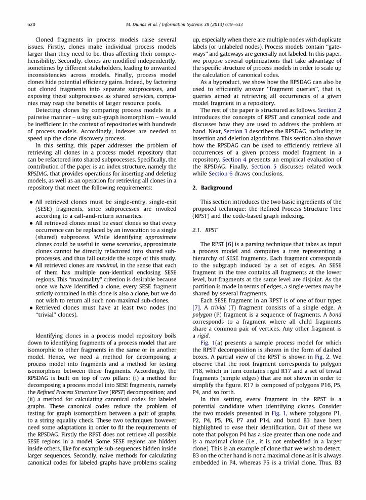
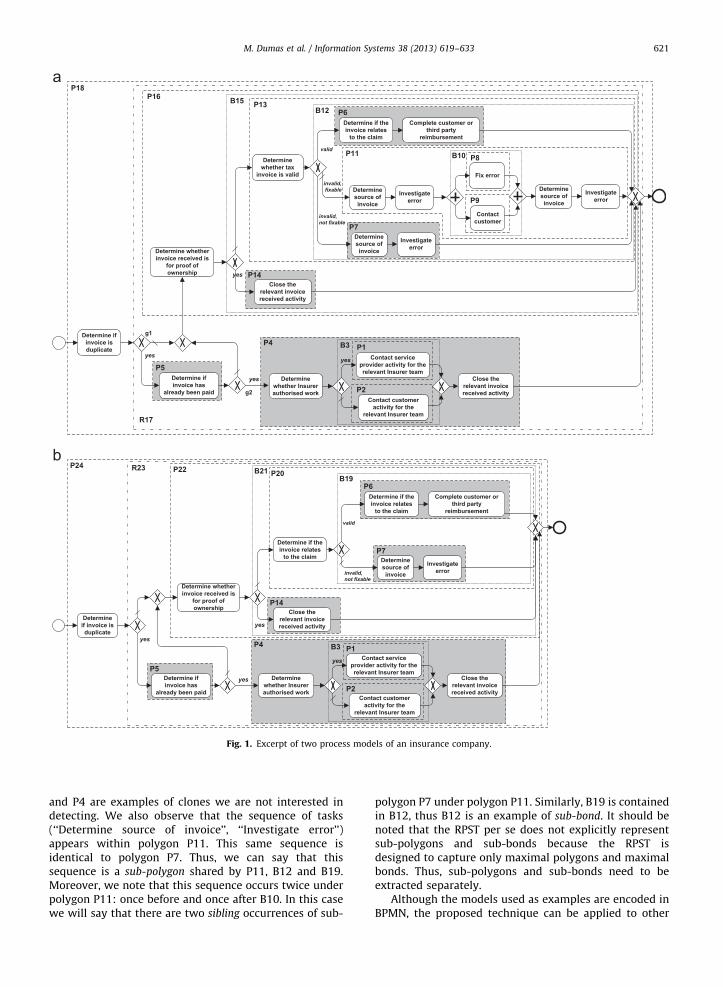
Fig. 1(a) presents a sample process model for whichthe RPST decomposition is shown in the form of dashedboxes. A partial view of the RPST is shown in Fig. 2. Weobserve that the root fragment corresponds to polygonP18, which in turn contains rigid R17 and a set of trivialfragments (simple edges) that are not shown in order tosimplify the figure. R17 is composed of polygons P16, P5,P4, and so forth.

In this setting, every fragment in the RPST is apotential candidate when identifying clones. Considerthe two models presented in Fig. 1, where polygons P1,P2, P4, P5, P6, P7 and P14, and bond B3 have beenhighlighted to ease their identification. Out of these wenote that polygon P4 has a size greater than one node andis a maximal clone (i.e., it is not embedded in a largerclone). This is an example of clone that we wish to detect.B3 on the other hand is not a maximal clone as it is alwaysembedded in P4, whereas P5 is a trivial clone. Thus, B3

Fig. 1. Excerpt of two process models of an insurance company.

M. Dumas et al. / Information Systems 38 (2013) 619–633 621

and P4 are examples of clones we are not interested indetecting. We also observe that the sequence of tasks(‘‘Determine source of invoice’’, ‘‘Investigate error’’)appears within polygon P11. This same sequence isidentical to polygon P7. Thus, we can say that thissequence is a sub-polygon shared by P11, B12 and B19.Moreover, we note that this sequence occurs twice underpolygon P11: once before and once after B10. In this casewe will say that there are two sibling occurrences of sub-

polygon P7 under polygon P11. Similarly, B19 is containedin B12, thus B12 is an example of sub-bond. It should benoted that the RPST per se does not explicitly representsub-polygons and sub-bonds because the RPST isdesigned to capture only maximal polygons and maximalbonds. Thus, sub-polygons and sub-bonds need to beextracted separately.

Although the models used as examples are encoded inBPMN, the proposed technique can be applied to other

M. Dumas et al. / Information Systems 38 (2013) 619–633622

graph-based modeling notations. To achieve this nota-tion-independence, we adopt the following graph-basedrepresentation of process models:

Definition 2.1 (Process Graph). A Process Graph is alabelled connected graph G¼ ðV ,E,lÞ, where:

�

Figper

V is the set of vertices.

� EDV � V is the set of directed edges (e.g. representing

control-flow relations).

� l : V-Sn is a labeling function that maps each vertex

to a string over alphabet S. We distinguish the follow-ing special labels: lðvÞ ¼ ‘‘start’’ and lðvÞ ¼ ‘‘end’’ arereserved for start events and end events respectively;lðvÞ ¼ ‘‘xor� split’’ is used for vertices representingxor-split (exclusive decision) gateways; similarlylðvÞ ¼ ‘‘xor� join’’, lðvÞ ¼ ‘‘and� split’’ and lðvÞ ¼

‘‘and� join’’ represent merge gateways, parallel splitgateways and parallel join gateways respectively. For atask node t, l(t) is the label of the task.

This definition can be extended to capture other typesof BPMN elements by introducing additional types of

nodes (e.g. a type of node for inclusive gateways, dataobjects etc.). Organizational information such as lanes andpools can be captured by attaching dedicated attributes toeach node (e.g. each node could have an attribute indicat-ing the pool and lane to which it belongs) [8]. In thispaper, we do not consider sub-processes, since each sub-process can be indexed separately for the purpose of cloneidentification.

. 3. (a) A sample graph, (b) its adjacency matrix, (c) its diagonal matrix wi

mutation of the augmented matrix.

Fig. 2. RPST of the process model in Fig. 1(a).

2.2. Canonical labeling of graphs

Our approach for graph indexing is an adaptation ofthe approach proposed in [9]. The adaptations we makerelate to two specificities of process models that differ-entiate them from the class of graphs considered in [9]: (i)process models are directed graphs; (ii) process modelscan be decomposed into an RPST.

Following the method in [9], our starting point is amatrix representation of a process graph encoding thevertex adjacency and the vertex labels, as defined below.

Definition 2.2 (Augmented Adjacency Matrix of a Process

Graph). Let G¼ ðV ,E,lÞ be a Process Graph, andv¼ ðv1, . . . ,v9V9Þ a total order over the elements of V. Theadjacency matrix of G, denoted as A, is a ð0,1Þ-matrix suchthat Ai,j ¼ 1 if and only if ðvi,vjÞ 2 E, where i,j 2 f1 . . . 9V9g.Moreover, let us consider a function h : Sn-N\f0,1g thatmaps each vertex label to a unique natural numbergreater than 1. The Augmented Adjacency Matrix M of G

is defined as: M ¼ diagð hðlðv1ÞÞ, . . . , hðlðv9V9ÞÞ ÞþA

Given the augmented adjacency matrix of a processgraph (or an SESE fragment therein), we can compute astring (hereby called a code) by concatenating the contentsof each cell in the matrix from left to right and from top tobottom. For illustration, consider graph G in Fig. 3(a),which is an abstract view of fragment B3 of the runningexample (cf. Fig. 1(a)). For convenience, next to each vertexwe show the unique vertex identifier (e.g. v1), the corre-sponding label (e.g. lðv1Þ ¼ ‘‘A’’), and the numeric valueassociated with the label (e.g. hðlðv1ÞÞ ¼ 2). Assuming theorder v¼ ðv1,v2,v3,v4Þ over the set of vertices, the matrixshown in Fig. 3(b) is the adjacency matrix of G. Fig. 3(c) isthe diagonal matrix built from hðlðvÞÞ whereas Fig. 3(d)shows the augmented adjacency matrix M for graph G. It isnow clear why 0 and 1 are not part of the codomain offunction h, i.e. to avoid clashes with the representation ofvertex adjacency. Fig. 3(e) shows a possible permutation ofM when considering the alternative order v0 ¼ ðv1,v4,v2,v3Þ

over the set of vertices.Next, we transform the augmented adjacency matrix

into a code by scanning from left-to-right and top-to-bottom. For instance, the matrix in Fig. 3(d) can berepresented as ‘‘2.1.1.0.0.3.0.1.0.0.4.1.0.0.0.5’’. This codehowever does not uniquely represent the graph. If wechose a different ordering of the vertices, we would obtaina different code. To obtain a unique code (called canonical

code), we need to pick the code that lexicographically‘‘precedes’’ all other codes that can be constructed froman augmented adjacency matrix representation of thegraph. Conceptually, this means that we have to consider

th the vertex label codes, (d) its augmented adjacency matrix, and (e) a

M. Dumas et al. / Information Systems 38 (2013) 619–633 623

all possible permutations of the set of vertices andcompute a code for each permutation, as captured in thefollowing definition.

Definition 2.3 (Graph Canonical Code). Let G be a processgraph, M the augmented adjacency matrix of G. The Graph

Canonical Code is the smallest lexicographical stringrepresentation of any possible permutation of matrix M,that is:

codeðMÞ ¼ strðPT MPÞ9P 2 P4 8Q 2P,

PaQ : strðPT MPÞ!strðQ T MQ Þ

where

�

P is the set of all possible permutations of the identitymatrix I9M9

�

strðNÞ is a function that maps a matrix N into a stringrepresentation.

Consider the matrices in Fig. 3(d) and (e). The code ofthe matrix in Fig. 3(e) is ‘‘2.0.1.1.0.5.0.0.0.1.3.0.0.1.0.4’’.This code is lexicographically smaller than the code ofthe matrix in Fig. 3(d) (‘‘2.1.1.0.0.3.0.1.0.0.4.1.0.0.0.5’’).If we explored all vertex permutations and constructedthe corresponding matrices, we would find that‘‘2.0.1.1.0.5.0.0.0.1.3.0.0.1.0.4’’ is the canonical code ofthe graph in Fig. 3(a).

Enumerating all vertex permutations is unscalable(factorial on the number of vertices). Fortunately, optimi-zations can be applied by leveraging the characteristics ofthe graphs at hand. Firstly, by exploiting the nature of thefragments in an RPST, we can apply the followingoptimizations:

�

The code of a polygon is computed in linear time byconcatenating the codes of its contained vertices in the(total) order implied by the control-flow. � The code of a bond is computed in linear time by

taking the entry gateway as the first vertex, the exitgateway as the last vertex, and all vertices in-betweenin lexicographic order based on their labels. Sincethese vertices in-between do not have any control-flow dependencies among them, duplicate labels donot pose a problem.

In the case of a rigid, we start by partitioning its verticesinto two subsets: vertices with distinct labels, and ver-tices with duplicate labels. Vertices with distinct labelsare deterministically ordered in lexicographic order.Hence we do not need to explore any permutationsbetween these vertices. Instead, we can focus on deter-ministically ordering vertices with duplicate labels. Dupli-cate labels in process models arise in two cases: (i) thereare multiple tasks (or events) with the same label;(ii) there are multiple gateways of the same type(e.g. multiple ‘‘xor-splits’’) that cannot be distinguishedfrom one another since gateways generally do not havelabels. To distinguish between multiple gateways, we

pre-process each gateway g by computing the tasks thatimmediately precede it and the tasks that immediatelyfollow it within the same rigid fragment, and in doing so,we skip other gateways found between gateway g andeach of its preceding (or succeeding) tasks. We thenconcatenate the labels of the preceding tasks (in lexico-graphic order) and the labels of the succeeding tasks(again in lexicographic order) to derive a new label sg.The sg labels derived in this way are used to ordermultiple gateways of the same type within the samerigid. Consider for example g1 and g2 in Fig. 1a and lets1¼ ‘‘Determine if invoice has already been paid’’,s2¼ ‘‘Determine whether invoice received is for proofof ownership’’ and s3¼ ‘‘Determine whether Insurerauthorized work’’. We have that sg1

¼ ‘‘s1:s2’’ whilesg2¼ ‘‘s1:s3:s2’’. Since s3 precedes s2, gateway g2 will

always be placed before g1 when constructing an aug-mented adjacency matrix for R17. In other words, we donot need to explore any permutation where g1 comesbefore g2. Even if task ‘‘Determine if invoice is duplicate’’precedes g1 this is not used to compute sg1

because thistask is outside rigid R17. To ensure unicity, verticeslocated outside a rigid should not be used to computeits canonical code.

A similar approach is used to order tasks with dupli-cate labels within a rigid. This ‘‘label propagation’’approach allows us to considerably reduce the numberof permutations we need to explore. Indeed, we only needto explore permutations between multiple vertices if theyhave identical labels and they are preceded and followedby vertices that also have the same labels. The worst-casecomplexity for computing the canonical code is stillfactorial, but on the size of the largest group of verticesinside a rigid that have identical labels and identicalpredecessors and successors’ labels.

3. Clone detection method

This section introduces the RPSDAG, including itsunderlying data structure, insertion and deletion algo-rithms and its support for ‘‘all-clone queries’’ and ‘‘frag-ment queries’’.

3.1. Index structure and clone detection

The RPSDAG is a directed acyclic graph representingthe union of the RPSTs of a collection of process models.The key feature of the RPSDAG is that each SESE fragmentis represented only once, even if it appears multiple timesin the RPST of a given process model or across multipleRPSTs. When a new process model is inserted into anRPSDAG, its RPST is computed and traversed bottom-up.For each fragment, it is checked whether this fragmentalready exists in the RPSDAG. If it does, the fragment isnot inserted, but instead, the existing fragment is reused.For instance, consider an RPSDAG constructed from theprocess model shown in Fig. 1a. Imagine that the processmodel in Fig. 1b is inserted into this RPSDAG, meaningthat the fragments in its RPST are inserted into theRPSDAG one by one from bottom to top. When the RPSTnode corresponding to polygon P4 is reached, we detect

M. Dumas et al. / Information Systems 38 (2013) 619–633624

that this fragment already exists. Rather than insertingthe fragment, an edge is created from its parent fragment(R23) to the existing node P4.

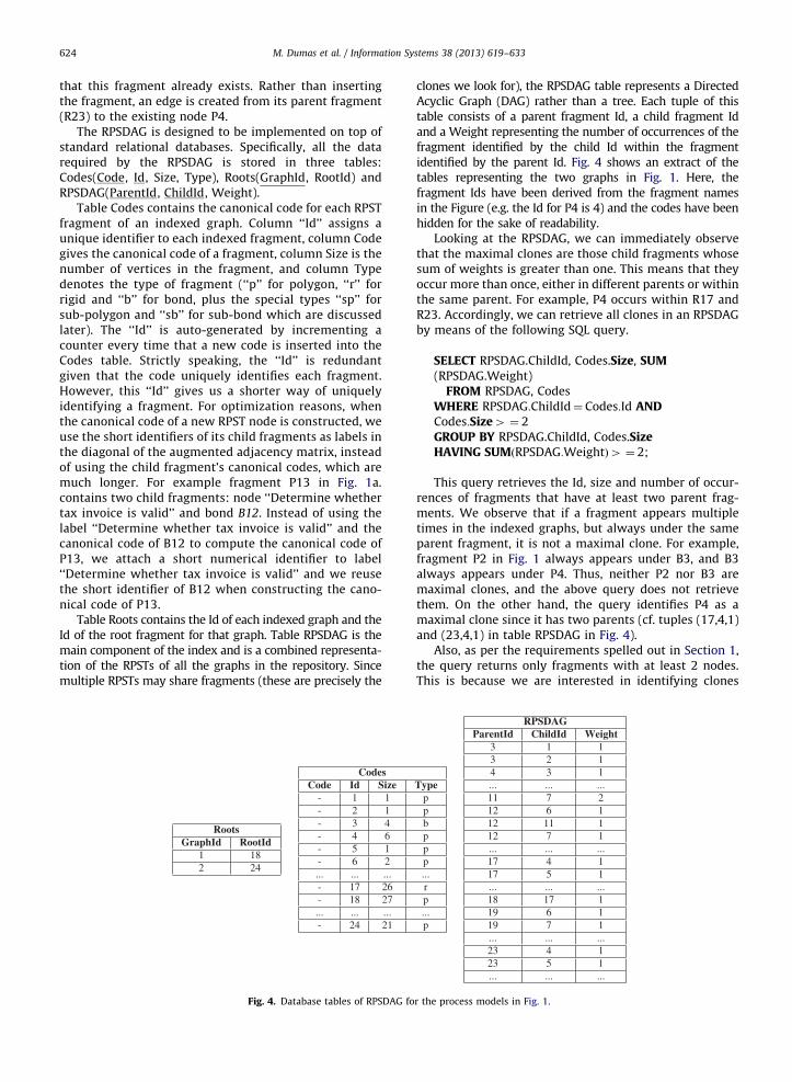
The RPSDAG is designed to be implemented on top ofstandard relational databases. Specifically, all the datarequired by the RPSDAG is stored in three tables:Codes(Code, Id, Size, Type), Roots(GraphId, RootId) andRPSDAG(ParentId, ChildId, Weight).

Table Codes contains the canonical code for each RPSTfragment of an indexed graph. Column ‘‘Id’’ assigns aunique identifier to each indexed fragment, column Codegives the canonical code of a fragment, column Size is thenumber of vertices in the fragment, and column Typedenotes the type of fragment (‘‘p’’ for polygon, ‘‘r’’ forrigid and ‘‘b’’ for bond, plus the special types ‘‘sp’’ forsub-polygon and ‘‘sb’’ for sub-bond which are discussedlater). The ‘‘Id’’ is auto-generated by incrementing acounter every time that a new code is inserted into theCodes table. Strictly speaking, the ‘‘Id’’ is redundantgiven that the code uniquely identifies each fragment.However, this ‘‘Id’’ gives us a shorter way of uniquelyidentifying a fragment. For optimization reasons, whenthe canonical code of a new RPST node is constructed, weuse the short identifiers of its child fragments as labels inthe diagonal of the augmented adjacency matrix, insteadof using the child fragment’s canonical codes, which aremuch longer. For example fragment P13 in Fig. 1a.contains two child fragments: node ‘‘Determine whethertax invoice is valid’’ and bond B12. Instead of using thelabel ‘‘Determine whether tax invoice is valid’’ and thecanonical code of B12 to compute the canonical code ofP13, we attach a short numerical identifier to label‘‘Determine whether tax invoice is valid’’ and we reusethe short identifier of B12 when constructing the cano-nical code of P13.

Table Roots contains the Id of each indexed graph and theId of the root fragment for that graph. Table RPSDAG is themain component of the index and is a combined representa-tion of the RPSTs of all the graphs in the repository. Sincemultiple RPSTs may share fragments (these are precisely the

RootsGraphId RootId

1 182 24

CodesCode Id Size- 1 1- 2 1- 3 4- 4 6- 5 1- 6 2... ... ...- 17 26- 18 27... ... ...- 24 21

Fig. 4. Database tables of RPSDAG fo

clones we look for), the RPSDAG table represents a DirectedAcyclic Graph (DAG) rather than a tree. Each tuple of thistable consists of a parent fragment Id, a child fragment Idand a Weight representing the number of occurrences of thefragment identified by the child Id within the fragmentidentified by the parent Id. Fig. 4 shows an extract of thetables representing the two graphs in Fig. 1. Here, thefragment Ids have been derived from the fragment namesin the Figure (e.g. the Id for P4 is 4) and the codes have beenhidden for the sake of readability.

Looking at the RPSDAG, we can immediately observethat the maximal clones are those child fragments whosesum of weights is greater than one. This means that theyoccur more than once, either in different parents or withinthe same parent. For example, P4 occurs within R17 andR23. Accordingly, we can retrieve all clones in an RPSDAGby means of the following SQL query.

Typppbppp...rp...p

r th

SELECT RPSDAG.ChildId, Codes.Size, SUM(RPSDAG.Weight)

FROM RPSDAG, CodesWHERE RPSDAG:ChildId¼ Codes:Id ANDCodes:Size4 ¼ 2GROUP BY RPSDAG.ChildId, Codes.SizeHAVING SUMðRPSDAG:WeightÞ4 ¼ 2;

This query retrieves the Id, size and number of occur-rences of fragments that have at least two parent frag-ments. We observe that if a fragment appears multipletimes in the indexed graphs, but always under the sameparent fragment, it is not a maximal clone. For example,fragment P2 in Fig. 1 always appears under B3, and B3always appears under P4. Thus, neither P2 nor B3 aremaximal clones, and the above query does not retrievethem. On the other hand, the query identifies P4 as amaximal clone since it has two parents (cf. tuples (17,4,1)and (23,4,1) in table RPSDAG in Fig. 4).

Also, as per the requirements spelled out in Section 1,the query returns only fragments with at least 2 nodes.This is because we are interested in identifying clones

e

RPSDAGParentId ChildId Weight

3 1 13 2 14 3 1... ... ...11 7 212 6 112 11 112 7 1... ... ...17 4 117 5 1... ... ...18 17 119 6 119 7 1... ... ...23 4 123 5 1... ... ...

e process models in Fig. 1.

M. Dumas et al. / Information Systems 38 (2013) 619–633 625

that can be refactored into separate subprocesses and isnot worth replacing single nodes with subprocesses. Forexample, even if there are two tuples with child Id 5 in theexample RPSDAG of Fig. 4, the query will not return cloneP5 as it has a single node.

3.2. Insertion

Algorithm 1 describes the procedure for inserting anew process graph into an indexed repository. Given aninput graph, the algorithm first computes its RPST withfunction ComputeRPST() which returns the RPST’s rootnode. Next, procedure InsertFragment is invoked on theroot node to update tables Codes and RPSDAG. Thisreturns the id of the root fragment. Finally, a tuple isadded to table Roots with the id of the inserted graph andthat of its root node.

Algorithm 1. Insert Graph.

procedure InsertGraphðGraph mÞ;

RPSTroot( ComputeRPSTðmÞ;

rid( InsertFragmentðrootÞ;

Roots( Roots [ fðNewIdðÞ,ridÞg // NewId() generates a fresh id;

Algorithm 2. Insert Fragment.

procedure InsertFragmentðRPSTf ) returns RPSDAGNodeId;

fRPST,RPSDAGNodeIdgC ( |;

foreach RPSTchild in GetChildrenðf Þ do

bC ( C [ fðchild,InsertFragmentðchildÞÞg;

code( ComputeCodeðf ,CÞ;

ðid,typeÞ ¼ InsertNodeðcode,f Þ;

foreach (cf,cid) in C do

weight ¼GetWeightðid,cidÞ;

RPSDAG( RPSDAG\fðid,cid,weightÞg [ fðid,cid,weightþ1Þg;

$

lif type¼ ‘‘p’’ then InsertSubPolygonsðid,code,f Þ;

else if type¼ ‘‘b’’ then InsertSubBondsðid,code,f Þ;

return id;

1 An LCS of strings S1 and S2 is a substring of both S1 and S2, which is

not contained in any other substring shared by S1 and S2. LCSs of size one

are not considered for obvious reasons. LCSs can efficiently be identified

using a suffix tree [10], see e.g. [11] for a survey of LCS algorithms

Procedure InsertFragment (Algorithm 2) inserts an RPSTfragment in table RPSDAG. This algorithm performs adepth-first search traversal of the RPST. Nodes are visitedin postorder, i.e. a node is visited after all its children havebeen visited. When a node is visited, its canonical code iscomputed – function ComputeCode – based on the topol-ogy of the RPST fragment and the codes of its children(except of course for leaf nodes whose labels are theircanonical codes). Next, procedure InsertNode is invoked toinsert the node in table Codes, returning its id and type.This procedure (Algorithm 3) first checks whether the nodealready exists in Codes via function GetIdSizeType(). If itexists, GetIdSizeType() returns the id, size and type asso-ciated with that code, otherwise it returns the tuple (0,0,‘‘’’).In this latter case, a fresh id is created for the node at hand,then its size and type are computed via functions Compu-teSize and ComputeType, and a new tuple is added in tableCodes. Function ComputeSize returns the sum of the sizesof all child nodes or 1 if the current node is a leaf. Once thenode id and type have been retrieved, procedure Insert-Fragment adds a new tuple in table RPSDAG for each

children of the visited node if that tuple did not alreadyexist, otherwise it increases its weight.

Algorithm 3. Insert Node.

procedure InsertNodeðStringcode,RPST f Þ returns

ðRPSDAGNodeId,StringÞ;

ðid,size,typeÞ ( GetIdSizeTypeðcodeÞ;

if ðid,size,typeÞ ¼ ð0,0,‘‘’’Þ then

id( NewIdðÞ;

size( ComputeSizeðcodeÞ;

type( ComputeTypeðf Þ;

Codes( Codes [ fðcode,id,size,typeÞg;

66666664return ðid,typeÞ;

Algorithm 4. Insert SubPolygons.

procedure

InsertSubPolygonsðRPSDAGNodeId id,String code,RPST f Þ;

foreach ðzcode,zid,zsize,ztypeÞ in Codes such that ztype¼ ‘‘p’’ 3 ‘‘sp’’

and zidaid do

fStringgLCS( ComputeLCSðcode,zcodeÞ;

foreach lcode in LCS doðlid,ltypeÞ ¼ InsertSubNodeðlcode,f Þ;

if lidaid then RPSDAG( RPSDAG [ fðid,lid,1Þg;

if lidazid then RPSDAG( RPSDAG [ fðzid,lid,1Þg;

foreach sid in GetChildrenIdsðlidÞ do

RPSDAG(

RPSDAG\fðid,sid,1Þ,ðzid,sid,1Þg [ fðlid,sid,1Þg;

$

InsertSubPolygonsðlid,lcodeÞ;

6666666666666664

666666666666666666664

If the visited node is a polygon, procedure InsertSub-Polygons is invoked at the end of InsertFragment. Proce-dure InsertSubPolygons is used to identify common sub-polygons and to factor them out as separate nodes in theRPSDAG. Let us consider again the example in Fig. 1. Asmentioned in Section 2, the sequence of activities (‘‘Deter-mine source of invoice’’, ‘‘Investigate error’’) – which isidentical to polygon P7 – occurs inside P11: once beforeand once after B10. These occurrences should be recog-nized as occurrences of polygon P7. Hence, P7 is a sub-

polygon shared by polygons P11, B12 and B19. ProcedureInsertSubPolygons identifies such sub-polygons andmaterializes them as explicit nodes in the RPSDAG. Thisexplains the presence of tuple (11,7,2) in the RPSDAG ofFig. 4.

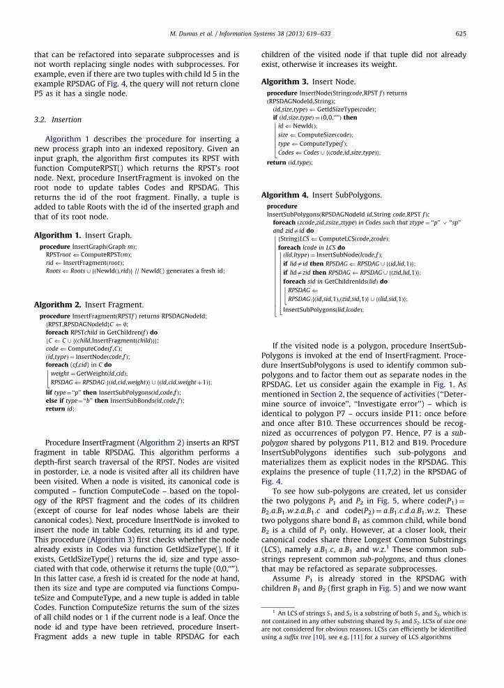
To see how sub-polygons are created, let us considerthe two polygons P1 and P2 in Fig. 5, where codeðP1Þ ¼

B2:a:B1:w:z:a:B1:c and codeðP2Þ ¼ a:B1:c:d:a:B1:w:z. Thesetwo polygons share bond B1 as common child, while bondB2 is a child of P1 only. However, at a closer look, theircanonical codes share three Longest Common Substrings(LCS), namely a:B1:c, a:B1 and w:z.1 These common sub-strings represent common sub-polygons, and thus clonesthat may be refactored as separate subprocesses.

Assume P1 is already stored in the RPSDAG withchildren B1 and B2 (first graph in Fig. 5) and we now want

Fig. 5. Two sub-polygons and the corresponding RPSDAG.

M. Dumas et al. / Information Systems 38 (2013) 619–633626

to store P2. We invoke procedure InsertFragment(P2) andadd a new node in the RPSDAG, with B1 as a child (secondgraph in Fig. 5). Since P2 is a polygon, we also need toinvoke InsertSubPolygons(P2). This procedure (Algorithm4) retrieves all polygons from Codes that are differentthan P2 (in our case there is only P1). Then, for each suchpolygon, it computes all the non-trivial LCSs between itscode and the code of the polygon being inserted. This isperformed by function ComputeLCS() that returns anordered list of LCSs starting from the longest one. In theexample at hand, the longest substring is a:B1:c. Thissubstring can be seen as the canonical code of a ‘‘shared’’sub-polygon between P2 and P1. To capture the fact thatthis shared sub-polygon is a clone, we insert a new nodeP3 in the RPSDAG with canonical code a:B1:c (unless sucha node already exists, in which case we reuse the existingnode) and we insert an edge from P2 to P3 and from P1 toP3. We also add a new tuple for P3 in Codes and set itstype to ‘‘sp’’ to keep track of sub-polygons (needed whenremoving a model from the repository—see Algorithm 5).If the node already exists, we change its type to ‘‘sp’’ inCodes. This is done by function InsertSubNode() which issimilar to InsertNode() with the only difference that itsets the type of the new node to ‘‘sp’’, while if the nodeexists it changes its type to ‘‘sp’’.

In order to avoid redundancy in the RPSDAG, the newnode P3 then ‘‘adopts’’ all the common children that it shareswith P2 and with P1. These nodes are retrieved by functionGetChildrenIds(), which simply returns the ids of all childnodes of P3: these will either be children of P1 or P2 or both.2

In our example, there is only one common child, namely B1,which is adopted by P3 (see third graph in Fig. 5).

It is possible that the newly inserted node also sharessub-polygons with other nodes in the RPSDAG. So, beforecontinuing to handle the remaining LCSs between P1 and P2,we invoke procedure InsertSubPolygons recursively over P3.In our example, the code of P3 shares the substring a:B1

2 They are children of one of the two polygons only, if the other

polygon is a sub-polygon of the former.

with both P2 and P1 (after excluding the code of P3 from thecodes of P2 and P1 since P3 is already a child of these twonodes). Thus we create a new node P4 with code a:B1 as achild of P3 and P2, and we make P4 adopt the common childB1 (see fourth graph in Fig. 5). We repeat the sameoperation between P3 and P1 but since this time P4 alreadyexists in the RPSDAG, we simply remove the edge betweenP1 and B1, and add an edge between P1 and P4 (fifth graph inFig. 5). Then, we resume the execution of InsertSubPoly-gons(P2) and move to the second LCS between P1 and P2, i.e.a:B1. Since this substring has already been inserted into theRPSDAG as node P4, nothing is done. This process ofsearching for LCSs is repeated until no more non-trivialcommon substrings can be identified. In the example athand, we also add sub-polygon w:z between P1 and P2 (lastgraph in Fig. 5). At this point, we have identified andfactored out all maximal sub-polygons shared by P1 andP2, and we can repeat the above process for other polygonsin the RPSDAG whose canonical code shares a commonsubstring with that of P1.

Sometimes there may be multiple overlapping LCSs ofthe same size. For example, given the codes of twopolygons a:b:c:d:e:f :a:b:c and a:b:c:k:b:c:d, if we extractone substring (say a:b:c), we can no longer extract thesecond one (b:c:d). In these cases we locally choose one ofthe overlapping LCS based on the number of occurrencesof an LCS within the two strings in question. If they havethe same number of occurrences, we randomly chooseone. In the example above, a:b:c has the same size of b:c:d

but it occurs three times, so we pick a:b:c and extract thecorresponding sub-polygon.

Procedure InsertSubPolygons also handles the caseswhere the polygon to be inserted is a sub-polygon orsuper-polygon of an existing polygon. These are justspecial cases of shared sub-polygon detection.

Coming back to Algorithm 2, if the node to be added isa bond, procedure InsertSubBonds is called in order toidentify common sub-bonds and factor them out asseparate nodes. Take for example bond B19 in Fig. 1b.This bond is actually a sub-bond of B12 in Fig. 1a, sinceB12 contains B19 plus P11. Thus we want to add a parent-

M. Dumas et al. / Information Systems 38 (2013) 619–633 627

child relation from B12 to B19 in the RPSDAG, and changethe type of B19 in Codes to ‘‘sb’’ (sub-bond).

Procedure InsertSubBonds is similar to InsertSubPoly-gons, except that instead of detecting sub-polygons usingComputeLCS, we detect sub-bonds. Detecting sub-bondsis simpler than detecting sub-polygons. Since the order ofthe children within a bond is irrelevant, we simply needto compute the intersection between the children of thebond being inserted and the set of children of eachindexed bond. If the size of this intersection is greaterthan one, it means that the bond being inserted shares asub-bond with an already indexed bond. Naturally, weonly compare the bond being inserted with an indexedbond if they have the same types of split and joinbehavior. For example, it does not make sense to find asub-bond shared between a bond that has XOR-splits atits ends, and a bond that has AND-splits at its end.

If we find that the intersection between the bond beinginserted B and an already indexed bond B0 contains at leasttwo nodes3 we have effectively found a sub-bond SB

consisting of the children shared between B and B0. Ifsub-bond SB overlaps with any sub-bond already indexedunder B0, then we do not insert it because we are notinterested in retrieving overlapping clones – if we did, oneof the two overlapping clones could not be extracted as ashared sub-process because the other clone would alreadycontain some of its elements. If on the other hand there isno overlap between SB and any of the existing sub-bondsunder B0, we insert SB under B0. The mechanism to insertsub-bond SB is the same as for sub-polygons, i.e. a newnode is created in the RPSDAG capturing the shared sub-bond. Given that procedure InsertSubBonds is very similarto InsertSubPolygons, we do not show its pseudo-code.

Sometimes, a fragment may be contained multipletimes in the same parent fragment, like for examplesub-polygon P7 which is contained twice within P11 inFig. 1. These sibling clones are captured by attribute‘‘Weight’’ to each edge of the RPSDAG, representing thenumber of times a child node occurs inside a given parentnode. A Weight greater than 1 indicates a case of siblingclones. Our implementation of the RPSDAG does not storethe attribute Weight for every edge in the RPSDAG butonly for edges that have a weight of at least two. Thisoptimization is achieved by separating the RPSDAG tableinto two tables: one containing edges with a weight ofone and another for edges with a weight greater than one.The rationale is that only a small fraction of edges have aweight greater than one. This is purely an implementa-tion-level optimization. At the conceptual level, we viewthe RPSDAG table as a single table.

3.3. Deletion

Algorithm 5 shows the procedure for deleting a graphfrom an indexed repository. This procedure relies onanother procedure for deleting a fragment, namely Dele-teFragment (Algorithm 6). The DeleteFragment procedure

3 A fragment of type bond contains at least two children, so we are

interested in intersections that contain at least two nodes.

performs a depth-first search traversal of the RPSDAG svisiting the nodes in post-order. Nodes with at most oneparent are deleted, because they correspond to fragmentsthat appear only in the deleted graph. Deleting a nodeentails deleting the corresponding ok in table Codes anddeleting all tuples in the RPSDAG table where the deletednode corresponds to the parent Id. If a fragment has twoor more parents, the traversal stops along that branchsince this node and its descendants must remain in theRPSDAG. After invoking procedure DeleteFragment, thegraph itself is deleted from table Roots through its root Id.

Algorithm 5. Delete Graph.

procedure DeleteGraphðGraphId midÞ;

RPSDAGNodeId rid( GetRootðmidÞ;

DeleteFragmentðridÞ;

Roots( Roots\fðmid,ridÞg;

CleanRPSDAGðÞ;

Algorithm 6. Delete Fragment.

procedure DeleteFragmentðRPSDAGNodeId fidÞ;

if 9fðpid,cid,weightÞ 2 RPSDAG : cid¼ fidg9r1 then

foreach ðpid,cid,weightÞ in RPSDAG where pid¼ fid do

DeleteFragmentðcidÞ;

RPSDAG( RPSDAG\fðpid,cid,weightÞg;

$

Codes( fðcode,id,size,typeÞ 2 Codes : idafidg;

66666664

Algorithm 7. Clean RPSDAG.

procedure CleanRPSDAGðÞ;

foreach ðpid,cid,weightÞ in RPSDAG where GetTypeðcidÞ 2 f‘‘sp’’,

‘‘sb’’} and fðpid2 ,cid,weight2Þ 2 RPSDAG : pid2apidg ¼+ do

if GetTypeðcidÞ ¼GetTypeðpidÞ then

foreach ccid 2 GetChildrenIdsðcidÞ do

weight ¼GetWeightðcid,ccidÞ;

RPSDAG(

RPSDAG\fðcid,ccid,weightÞg [ fðpid,ccid,weightÞg;

66664

66666664else

bRestoreTypeðcidÞ;

6666666666666664

Before completing the DeleteGraph procedure, proce-dure CleanRPSDAG is triggered (see Algorithm 7). Thisprocedure cleans up the RPSDAG by removing those sub-fragments (i.e. sub-polygons and sub-bonds) which havebeen added with procedures InsertSubPolygons and Insert-SubBonds but that are now left with a single parent as partof executing DeleteGraph. There is no reason to keep thesesub-fragments in the RPSDAG since they may prevent theidentification of further sub-fragments within their parents,as new nodes are inserted into the RPSDAG. For example,let us consider the RPSDAG that we created from the twomodels in Fig. 1. As pointed out before, this RPSDAGcontains an edge between B12 and B19 (the latter being asub-bond of the former). Now, let us assume we remove themodel in Fig. 1b from our repository. Since B19 has twoparents, namely B12 in model a and P20 in model b, B19 isnot deleted by procedure DeleteGraph. However, this nodewas a sub-fragment which is now left with a single parentof the same type (i.e. a bond). Thus, we also need to removethis sub-fragment from the RPSDAG. In doing so, we let its

M. Dumas et al. / Information Systems 38 (2013) 619–633628

only parent adopt this node’s children, P6 and P7 in ourexample. In other words, we revert the effects of theadoption that we did when creating a sub-polygon orsub-bond. After this operation, B12 has again its threeoriginal children: P6, P7 and P11. Any combination of thesechildren may later be used to create new sub-fragments asnew nodes are inserted into the RPSDAG.

There is also another case which requires cleaning. If asub-fragment is left with a single parent after Delete-Graph, but the parent’s type is different than that of thesub-fragment, it means this sub-fragment corresponds toan original polygon (bond) which has been retyped as asub-polygon (sub-bond) after procedure InsertSubPoly-gon (InsertSubBond). In this case CleanRSPDAG invokesfunction RestoreType() to restore the original type of thisfragment (e.g. if the type is ‘‘sp’’ it is changed to ‘‘p’’).Consider again the example of B19 and now assume weremove the model in Fig. 1a from our repository. Afterthis, B19 is left with one parent only, namely P20 which isa polygon. Thus, B19’s type is changed back to ‘‘b’’.

3.4. Complexity

The deletion algorithm performs a depth-first search,which is linear on the size of the graph being deleted.Similarly, the insertion algorithm traverses the insertedgraph in linear time. Then, for each fragment to be inserted,it computes its code. Computing the code is linear on thesize of the fragment for bonds and polygons, while forrigids it is factorial on the largest number of vertices insidethe rigid that share identical labels, as discussed in Section2.2.4 If the fragment is a polygon, we compute all LCSsbetween this polygon and all other polygons in theRPSDAG. Using a suffix tree, this operation is linear on thesum of the lengths of all polygons’ canonical codes. If thefragment is a bond, we compute all non-empty intersec-tions between the children of this bond and those of allother bonds. Using a hash table, this operation is linear onthe sum of the number of children of all bonds.

3.5. Correctness and completeness

The correctness of the proposed method for clonedetection follows from the following observations:

�

A node in the RPSDAG corresponds either to a node inthe RPST of an indexed model, or to a sub-polygon or asub-bond. � The RPST decomposition separates the input process

graph into SESE fragments that are either disjoint orhave a containment relationship.

� Sub-polygons and sub-bonds are SESE fragments and

the insertion algorithm ensures that the sub-polygons(resp. sub-bonds) that appear under a given polygon(bond) are disjoint and are contained by their parentnode in the RPSDAG (i.e. the parent polygon or bond).

4 A tighter complexity bound for this problem is given in [12].

These observations imply that every node in theRPSDAG is an SESE fragment and that every pair of modelfragments indexed in the RPSDAG are either disjoint or ina containment relation. Moreover, we only detect max-imal clones, meaning that if a clone C is contained in aclone C0, then C0 is not returned as a clone. Hence, the setof identified clones are disjoint SESE fragments.

The completeness of the proposed method for clonedetection stems from the following observations:

�

arb

nod

The RPST decomposition can be constructed for anyprocess model [7].5

�

The RPST decomposition contains one node per SESEsubgraph in the original graph, except for SESE sub-graphs of type polygon that are directly containedinside another polygon (i.e. sub-polygons) and SESEregions of type bond directly contained inside anotherbond (i.e. sub-bonds). The RPSDAG then extracts thesesub-polygons and sub-bonds when it is detected thattwo indexed polygons (bonds) share a common sub-polygon (sub-bond). Sub-polygons are detected using alongest common substring algorithm, thus ensuringthat maximal-sized shared sub-polygons are identified.

3.6. Fragment query

The proposed index can also be used to identify allgraphs in a repository that contain a query graph. Bybuilding the RPSDAG first, we can perform this operationefficiently as opposed to using subgraph isomorphismcheck, which is NP-complete [13]. In other words, we shiftthe bulk of the computational complexity from run-time(query execution) to design-time (repository creation).

Algorithm 8. Fragment Query.

procedure FragmentQueryðRPSDAGNodeId idÞ returns

fRPSDAGNodeId,RPSDAGNodeIdg;

fRPSDAGNodeId,RPSDAGNodeIdgMP(+;

foreach ðpid,cid,weightÞ in RPSDAG where cid¼ id do

R( GetRootIdsðpidÞ;

foreach rid in R do

bMP( MP [ fðGetGraphIdðridÞ,pidÞg;

66664if MP¼+ then

bMP( fðGetGraphIdðidÞ,idÞg;

return MP;

Algorithm 9. GetRootIds.

procedure GetRootIdsðRPSDAGNodeIdidÞ returns fRPSDAGNodeIdg;

fRPSDAGNodeIdgR(+;

foreach ðpid,cid,weightÞ in RPSDAG where cid¼ id do

bR( R [ GetRootIdsðpidÞ;

if R¼+ then

bR( fidg;

return R;

5 Specifically, [7] shows that an RPST can be constructed for any

itrary directed graph such that every node is on a path from a source

e to a sink node, which is a basic property of process models.

M. Dumas et al. / Information Systems 38 (2013) 619–633 629

The execution of a query (cf. Algorithm 8) takes afragment id as input, and returns the id of all models thequery fragment occurs in, and for each model, also the idof the parent fragment containing the query fragment. Inthis way we can locate the query fragment exactly withineach model satisfying the query. To do so, we first retrievethe root fragment id of all graphs containing the inputfragment by traversing the RPSDAG upwards from theinput fragment (function GetRootIds()). Then for each rootid we retrieve the corresponding model id from tableRoots using function GetGraphId(), which returns 0 if thegraph does not exist. Algorithm 8 assumes the id of thequery fragment is known. Otherwise, we can retrieve itfrom table Codes.

4. Evaluation

This section reports on a series of tests to evaluate theperformance of the RPSDAG as well as the usefulness ofclone detection in practical settings.

4.1. Evaluation dataset

We evaluated the RPSDAG using four datasets:

�

TabMo

D

S

In

B

B

S

In

B

B

S

In

B

B

The collection of SAP R3 reference process models [14]

� A model repository obtained from Suncorp, Australia’s

largest insurance company.

� Two collections from the IBM BIT process library [15],

namely collections A and B3. In the BIT process librarythere are five collections (A, B1, B2, B3 and C). Weexcluded collections B1 and B2 because they are ear-lier versions of B3, and collection C because it is a mixof models from different sources and as such it doesnot contain any clones.

The SAP repository contains 595 models with sizesranging from 5 to 119 nodes (average 22.28, median 17).The insurance repository contains 363 models rangingfrom 4 to 461 nodes (average 27.12, median 19). The BITcollection A contains 269 models ranging from 5 to 47nodes (average 17.01, median 16) while collection B3contains 247 models with 5 to 42 nodes (average 12.94,median 11). The examples in Fig. 1 are extracts of the

le 1del insertion times (in ms).

ataset min max avg

AP 4 85 20

surance 5 1722 32

IT A 3 58 12

IT B3 5 467 14

AP 4 482 97

surance 26 4402 126

IT A 18 128 41

IT B3 5 150 33

AP 10 859 232

surance 81 5043 295

IT A 71 226 129

IT B3 15 192 75

insurance models with node labels altered to protectconfidentiality.

4.2. Performance evaluation

We first evaluated the insertion times. Obviouslyinserting a new model into a nearly-empty RPSDAG is lesscostly than doing so in an already populated one. To factorout this effect, we randomly split each dataset as follows:One third of the models were used to construct an initialRPSDAG and the other two-thirds were used to measureinsertion times. In the SAP repository, 200 models wereused to construct an initial RPSDAG. Constructing theinitial RPSDAG took 26 s. In the insurance companyrepository, the initial RPSDAG contained 121 models andits construction took 26 s. For the BIT collections A and B3,90 and 82 models respectively were used for constructingthe initial RPSDAG. Constructing the initial RPSDAGs took8.6 s for collection A and 6.1 s for collection B3. All testswere conducted on a PC with a dual core Intel processor,1.8 GHz, 4 GB memory, running Microsoft Windows 7 andOracle Java Virtual Machine v1.6. The RPSDAG was imple-mented as a Java console application on top of MySQL 5.1.Each test was run 10 times and the execution timesobtained across the ten runs were averaged.

Table 1 summarizes the insertion time per model foreach collection (min, max, avg., std. dev., and 90th percen-tile). All values are in milliseconds. These statistics are givenfor three cases: without sub-polygon nor sub-bond clonedetection, with sub-polygon clone detection, and with bothsub-polygon and sub-bond clone detection. Herewith, weuse the term sub-fragment clone detection to refer to bothsub-polygon and sub-bond clone detection collectively.

We observe that the average insertion time per modelis 3–5 times larger when sub-polygon is performed. Thisoverhead comes from the step where we compare apolygon being inserted with each already-indexed poly-gon and we compute the longest-common substring oftheir canonical codes. As mentioned earlier, this operationcould be optimized at the implementation level by storingall the indexed polygons in a suffix tree [10]. Sub-bonddetection also introduces a visible overhead because ofthe step where an inserted bond is compared against each

std l90

14 40 No sub-fragments

113 49

9 23

9 28

81 202 Sub-polygons only

291 222

20 59

24 69

124 398 Sub-bonds þ sub-polygons

365 390

40 187

33 115

Table 2Total refactoring gain without and with sub-fragment refactoring.

Dataset No sub-fragments With sub-polygons With sub-polygons þ sub-bonds

Nr. clones gain Nr. clones gain Nr. clones gain

SAP 304 1359 (10.3%) 490 1859 (14%) 563 2261 (17.1%)

Insurance 108 395 (4%) 280 884 (9%) 302 933 (9.5%)

BIT A 57 195 (4.3%) 174 384 (8.4%) 178 391 (8.5%)

BIT B3 19 208 (6.5%) 49 259 (6.6%) 61 293 (9.2%)

6 If a clone appears multiple times under the same parent node in

the RPSDAG (sibling clones), this should be counted as multiple

occurrences.

M. Dumas et al. / Information Systems 38 (2013) 619–633630

indexed bond. This latter step could be optimized byusing bitsets to represent the set of children of each bond.

Despite the fact that the tool implementation does notincorporate these optimizations, the average executiontimes remain in the order of tens to hundreds of milli-seconds across all model collections even with sub-poloygon and sub-bond detection. The highest averageinsertion time (295 ms) is observed for the Insurancecollection. This collection contains some models withlarge rigid components in their RPST. In particular, onemodel contained a rigid component in which two tasklabels appeared nine times each – i.e. nine tasks had oneof these labels and nine tasks had the other – and thesetasks were all preceded by the same gateway. Puttingaside this extreme case, all insertion times were underone second and in 90% of the cases (l90), the insertiontimes in this collection were under 50 ms without sub-fragment detection and 400 ms with sub-fragment detec-tion. Thus we can conclude that the proposed techniquescales up to real-sized model collections.

As explained in Section 3, once the models areinserted, we can find all clones with an SQL query. Thequery to find all clones with at least two nodes andoccurring at least twice from the SAP reference modelstakes 75 ms on average, 90 ms for the insurance models,118 and 116 ms for the BIT collections A and B3.

Finally, we evaluated the performance of the RPSDAGfor handling fragment queries. To this end, we randomlyselected model fragments of sizes from five to 15 nodesfrom the SAP repository. In other words, for each frag-ment size (from 5 to 15), we randomly selected a frag-ment among all fragments of this size in the repository.For each fragment, we ran a query to retrieve all occur-rences of this fragment in the collection of models. Eachquery was executed five times and the execution timeswere averaged. The recorded average execution timesranged from 15 to 35 ms, with an average of 24 ms anda std. dev. of 6 ms.

4.3. Refactoring gain

One of the main applications of clone detection is torefactor the identified clones as shared subprocesses inorder to reduce the size of the model collection andincrease its navigability. In order to assess the benefit ofrefactoring clones into subprocesses, we define the fol-lowing measure.

Definition 4.1. The refactoring gain of a clone is thereduction in number of nodes obtained by encapsulating

that clone into a separate subprocess, and replacing everyoccurrence of the clone with a task that invokes thissubprocess. Specifically, let S be the size of a clone, and N

the number of occurrences of this clone.6 Since alloccurrences of a clone are replaced by a single occurrenceplus N subprocess invocations, the refactoring gain is:S � N�S�N.

Given a collection of models, the total refactoring gain isthe sum of the refactoring gains of the clones of non-trivial clones (size Z2) in the collection.

It should be noted that when a sub-bond is refactoredout, we need to introduce an additional split and a join inthe refactored sub-bond in order to separate it from theparent bond. Accordingly, in the case of sub-bonds, therefactoring gain is defined as: S � N�S�N�2.

Table 2 summarizes the total refactoring gain for eachmodel collection. The first two columns correspond to thetotal number of clones detected and the total refactoringgain without any sub-fragment refactoring. The third andfourth column show number of clones and refactoring gainwith sub-polygon refactoring. Finally, the last two columnsgive the number of clones and gain attained with both sub-polygon and sub-bond refactoring. The table shows that asignificant number of clones can be found in all modelcollections and that the size of these model collections couldbe reduced by 8.5-17% if clones were factored out intoshared subprocesses. The table also shows that sub-fragmentclone detection adds significant value to the clone detectionmethod. For instance, in the case of the insurance models,we obtain over twice more clones and twice more refactor-ing gain when sub-fragment clone detection is performed.The results demonstrate the potential usefulness of detectingand refactoring both sub-polygons and sub-bonds.

Sibling clones – i.e. identical fragments appearingunder the same parent node in the RPSDAG – representedonly a negligible fraction of all clones (seven siblingclones in the SAP repository, one in the Insurance repo-sitory, none in the IBM repositories).

Table 3 shows more detailed statistics of the clonesfound with sub-fragment detection (including both sub-polygons and sub-bonds). The first three columns givestatistics about the sizes of the clones found, the nextthree columns refer to the frequency (number of occur-rences) of the clones, and the last three correspond to theefactoring gain. We observe that while the average clone

Table 3Statistics of detected clones (with sub-fragment detection).

Dataset Size # occurrences Refactoring gain

avg max std.

dev.

avg max std.

dev.

avg max std.

dev.

SAP 5.01 41 4.02 2.37 11 0.89 4.02 44 5.82

Insurance 3.73 32 3.20 2.71 41 3.05 3.09 79 7.46

BIT A 3.02 16 2.10 2.74 9 1.28 2.20 15 3.10

BIT B3 3.36 9 1.51 3.69 20 3.39 4.80 37 8.09

Table 4Refactoring clones with size of at least four nodes (with sub-fragment

detection).

Dataset No. Clones Refactoring gain

SAP 300 1949 (14.7%)

Insurance 107 613 (6.25%)

BIT A 39 234 (5.11%)

BIT B3 27 171 (5.36%)

M. Dumas et al. / Information Systems 38 (2013) 619–633 631

size is relatively small (3–5 nodes), there are also largeclones with sizes of 30þ nodes.

It might be desirable not to refactor out small clones,as it would add complexity and fragmentation in themodel collection by introducing many ‘‘small’’ subpro-cesses and making the dataset more difficult to navigate.The smallest process model in the evaluated datasets has4 nodes. Thus, it would make sense to refactor out onlyclones that have at least 4 nodes in order not to introducesubprocesses that are smaller than those that processmodelers would normally define themselves. Table 4shows the refactoring gains obtained if we only considerclones with at least four nodes. We observe that refactor-ing out only clones of at least four nodes still gives us asignificant amount of refactoring gain. For the SAP collec-tion we still identify 293 clones out of 555 clones (withsub-fragment detection), leading to a refactoring gain of14.7% (versus 17.1% if we consider all clones).

5. Related work

This paper is an extended version of a previous con-ference paper [16]. The extensions include the ability todetect sub-bond clones and sibling clones, as well as theapplication of the RPSDAG to handle fragment queries.The experimental evaluation was extended to assess theperformance of the extended RPSDAG and of the queryprocessing, and to assess the usefulness of sub-bond andsibling clone detection. Below, we review related workalong the following areas: (i) clone detection in softwarerepositories; (ii) clone detection in model-driven engi-neering; (iii) graph database indexing; (iv) refactoringtechniques for process model repositories; and (v) querylanguages for process model repositories.

5.1. Clone detection in software repositories

Clone detection in software repositories has been anactive field for several years. According to [17], approaches

can be classified into: textual comparison, token compar-ison, metric comparison, abstract syntax tree (AST) compar-ison, and program dependence graphs (PDG) comparison.The latter two categories are close to our problem, as theyuse a graph-based representation. In [18], the authorsdescribe a method for clone detection based on ASTs. Themethod applies a hash function to subtrees of the AST inorder to distribute subtrees across buckets. Subtrees in thesame bucket are compared by testing for tree isomorphism.This work differs from ours in that RPSTs are not perfecttrees. Instead, RPSTs contain rigid components that areirreducible and need to be treated as subgraphs—thus treeisomorphism is not directly applicable.

Code clone detection using PDGs has been investigatedin [19]. The PDG is a directed graph where nodes corre-spond to lexer tokens, and edges correspond to control,data and reference dependencies. A subgraph isomorph-ism algorithm is used for clone detection. This techniqueis unsuitable for online processing due to performanceand memory requirements [17]. In contrast, we employcanonical codes instead of pairwise subgraph isomorph-ism detection. The bottleneck is that we have to poten-tially consider all permutation of gateways in a rigidcomponent in order to construct the canonical code. Ourexperiments show however that this can be achieved insub-second times even for large process models. Anotherdifference between our approach and those based on PDGis that we take advantage of the RPST in order todecompose the process graph into SESE fragments, allow-ing us to focus on smaller fragments at once.

5.2. Clone detection in model-driven engineering

Work on clone detection has also been undertaken in thefield of model-driven engineering. [20] describes a methodfor detecting clones in large repositories of Simulink/Targe-tLink models from the automotive industry. Models arepartitioned into connected components and compared pair-wise using a heuristic subgraph matching algorithm. Again,the main difference with our work is that we use canonicalcodes instead of subgraph isomorphism detection.

In [21], the authors describe two methods for exactand approximate matching of clones for Simulink models.In the first method, they apply an incremental, heuristicsubgraph matching algorithm. In the second approach,graphs are represented by a set of vectors built fromgraph features: e.g. path lengths, vertex in/out degrees,etc. An empirical study shows that this feature-basedapproximate matching approach improves pre-processingand running times, while keeping a high precision. How-ever, this data structure does not support incrementalinsertions/deletions.

5.3. Graph database indexes

Our work is also related to graph database indexingand is inspired by [9]. Other related indexing techniquesfor graph databases include GraphGrep [13]—an indexdesigned to retrieve paths in a graph that match a regularexpression. This problem however is different from that ofclone detection since clones are not paths (except for

M. Dumas et al. / Information Systems 38 (2013) 619–633632

polygons). Another related index is the closure-tree [22].Given a graph G, the closure-tree can be used to retrieveall indexed graphs in which G occurs as a subgraph. Wecould use the closure tree to index a collection of processgraphs so that when a new graph is inserted we can checkif any of its SESE regions appears in an already indexedgraph. However, the closure tree does not directly retrievethe exact set of graphs where a given subgraph occurs.Instead, it retrieves a ‘‘candidate set’’ of graphs. An exactsubgraph isomorphism test is then performed againsteach graph in the candidate set. In contrast, by storingthe canonical code of each SESE region, the RPSDAGobviates the need for this subgraph isomorphism testing.

In [23], we described an index to retrieve processmodels in a repository that exactly or approximatelymatch a given model fragment. In this approach, processmodels are represented as Petri nets and paths in theprocess models are used as index features. Given acollection of models, a Bþ tree is used to reduce thesearch space by discarding those models that do notcontain any path of the query model. The remainingmodels are tested for subgraph isomorphism.

5.4. Refactoring process model repositories

In [24], eleven process model refactoring techniques,called ‘‘smells’’, are identified and evaluated. Extractingprocess fragments as subprocesses is one of the techniquesidentified. Our work addresses the problem of identifyingopportunities for such ‘‘fragment extraction’’. Recent workhas shown that several other types of refactoring opportu-nities can be semi-automatically identified by computingsimilarity metrics on model fragments [25]. Specifically, thisrelated work suggests to identify refactoring opportunities bycomputing similarity metrics on every pair of (SESE) frag-ments within a given repository of process models. Thisapproach can be used in particular to identify ‘‘subprocessextraction’’ opportunities, including subprocess extractionopportunities where the refactored fragments are not iden-tical. However, in doing so, the approach leads to many ‘‘falsepositives’’, and thus requires additional filters or fine-tuning.Our approach is less general, but does not produce falsepositives: Every clone detected by our technique constitutesa subprocess extraction opportunity. Also, our approachexplicitly aims to reduce computational overhead, while thisis not a concern in the work reported in [25]. In other words,our technique strikes different tradeoffs and is potentiallycomplementary to the techniques presented in [25].

5.5. Querying process model repositories

In this paper we showed how the RPSDAG can be usedto efficiently query a repository for the existence of agiven process fragment. Two major research efforts havebeen dedicated to the development of query languages forprocess model repositories: BP-QL and BPMN-Q. BP-QL[26] is a graphical query language based on an abstractrepresentation of BPEL, which is supported by a formalmodel of graph grammars for query processing. BP-QL canbe used to query process specifications written in BPELrather than possible executions, and ignores the run-time

semantics of certain BPEL constructs such as conditionalexecution and parallel execution.

BPMN-Q [27,28] is also a visual query language whichextends a subset of the BPMN modelling notation andsupports graph-based query processing. Similarly to BP-QL, BPMN-Q captures the structural relationshipsbetween tasks. In [29], the authors explore the use of aninformation retrieval technique to derive similarities ofactivity names, and develop an ontological expansion ofBPMN-Q to tackle the problem of querying businessprocesses that are developed with different terminologies.

The above works do not focus on efficient querying butrather on how to formulate process model queries graphi-cally, and on how to parse these queries. As such, these workscomplement our work on fragment querying by providing aninterface through which users can submit queries.

6. Conclusion

We presented a technique to index process models inorder to identify duplicate SESE fragments (clones) thatcan be refactored into shared subprocesses. The proposedindex, namely the RPSDAG, combines a method fordecomposing process models into SESE fragments (theRPST decomposition) with a method for generating aunique string to identify a labeled graph (canonicalcodes). Canonical codes are used to determine whetheran SESE fragment in a model appears elsewhere in thesame or in another model.

The RPSDAG has been implemented and tested usingprocess model repositories from industrial practice. Inaddition to demonstrating the scalability of the RPSDAG,the experimental results show that a significant numberof non-trivial clones can be found in industrial processmodel repositories. In one repository, more than 560 non-trivial clones were found. By refactoring these clones, theoverall size of the repository is reduced by around 17%,which arguably would enhance the repository’s maintain-ability. We also showed that the RPSDAG can be used toefficiently answer ‘‘fragment queries’’, that is, retrievingall occurrences of a given model fragment in a repository.

In separate work [30], we adapted the RPSDAG to dealwith concurrent editing and change propagation in thecontext of repositories of versioned process models. Con-current editing is handled by allowing modelers to obtainlocks at the level of individual fragments of a processmodel as opposed to locking an entire model. This opera-tion corresponds to placing a lock on a node of theRPSDAG. Change propagation is achieved by allowingmodelers to determine, on a fragment-by-fragment basis,whether or not changes made in a version of a modelshould be propagated to other versions.

A standalone release of the RPSDAG implementation,together with sample models, is available at: http://apromore.org/tools. The RPSDAG implementation can be opti-mized in several ways: (i) by using suffix trees for identifyingthe longest common substrings between the code of aninserted polygon and those of already-indexed polygons;(ii) by storing the canonical codes of each fragment in a hashindex in order to speed up retrieval; (iii) by using the Nautylibrary for computing canonical codes (http://cs.anu.edu.au/

M. Dumas et al. / Information Systems 38 (2013) 619–633 633

�bdm/nauty). Nauty implements several optimizations thatcould complement those described in Section 2.2.

One issue that arises when extracting clones intoshared subprocesses is that of giving meaningful labelsto the subprocesses. To assist analysts in this task, it maybe desirable to automatically suggest possible labels forthe sub-processes to be extracted. Such suggestions couldbe derived by analyzing the labels of the tasks inside theclone and using meronymy relations to compute aggre-gate labels as investigated in [31].

Another avenue for future work is to extend theproposed technique in order to identify approximate

clones. This has applications in the context of processstandardization, when analysts seek to identify similarbut non-identical fragments and to replace them withstandardized fragments in order to increase the homo-geneity of work practices.

Acknowledgments

This research is funded by the Estonian Science Founda-tion and ERDF via the Estonian Centre of Excellence inComputer Science (Uba, Dumas and Garcıa-Banuelos), andby ARC Linkage Grant ‘‘LP110100252’’ and NICTA QueenslandLab (La Rosa).

References

[1] M. Rosemann, Potential pitfalls of process modeling: part A,Business Process Management Journal 12 (2) (2006) 249–254.

[2] H.A. Reijers, R.S. Mans, R.A. van der Toorn, Improved modelmanagement with aggregated business process models, Data andKnowledge Engineering 68 (2) (2009) 221–243.

[3] M. La Rosa, M. Dumas, R. Dijkman, Business process model mer-ging: an approach to business process consolidation, ACM Transac-tions on Software Engineering and Methodology, in press.

[4] R. Dijkman, M. La Rosa, H. Reijers, Managing large collectionsof business process models—current techniques and challenges,Computers in Industry 63 (2) (2012) 91–97.

[5] R. Koschke, Identifying and removing software clones, in: SoftwareEvolution, Springer, 2008, pp. 15–36.

[6] J. Vanhatalo, H. Volzer, J. Koehler, The refined process structuretree, Data and Knowledge Engineering 68 (9) (2009) 793–818.

[7] A. Polyvyanyy, J. Vanhatalo, H. Volzer, Simplified computation andgeneralization of the refined process structure tree, in: WebServices and Formal Methods—7th International Workshop,WS-FM 2010, Hoboken, NJ, USA, September 16–17, 2010. RevisedSelected Papers, vol. 6551, Lecture Notes in Computer Science,Springer, 2010, pp. 25–41.

[8] M. La Rosa, H. Reijers, W. van der Aalst, R. Dijkman, J. Mendling,M. Dumas, L. Garcia-Banuelos, APROMORE: an advanced processmodel repository, Expert Systems with Applications 38 (6) (2011)7029–7040.

[9] D.W. Williams, J. Huan, W. Wang, Graph database indexing usingstructured graph decomposition, in: Proceedings of the 23rd Inter-national Conference on Data Engineering, ICDE 2007, April 15–20,2007, The Marmara Hotel, Istanbul, Turkey, IEEE Computer Society,2007, pp. 976–985.

[10] E. Ukkonen, On-line construction of suffix trees, Algorithmica 14(3) (1995) 249–260.

[11] D. Gusfield, Algorithms on Strings, Trees and Sequences: ComputerScience and Computational Biology, Cambridge University Press, 1997.

[12] L. Babai, Monte-Carlo Algorithms in Graph Isomorphism Testing,Technical Report, D.M.S. No. 79-10, Universite de Montreal, Dep. demathematiques et de statistique, 1979.

[13] D. Shasha, J.T.-L. Wang, R. Giugno, Algorithmics and applications oftree and graph searching, in: Proceedings of the Twenty-first ACMSIGACT-SIGMOD-SIGART Symposium on Principles of DatabaseSystems, June 3–5, Madison, Wisconsin, USA, ACM, 2002, pp. 39–52.

[14] G. Keller, T. Teufel, SAP R/3 Process Oriented Implementation:Iterative Process Prototyping, Addison-Wesley, 1998.

[15] D. Fahland, C. Favre, B. Jobstmann, J. Koehler, N. Lohmann, H. Volzer,K. Wolf, Instantaneous soundness checking of industrial businessprocess models, in: Business Process Management, vol. 5701, LectureNotes in Computer Science, Springer, 2009, pp. 278–293.

[16] R. Uba, M. Dumas, L. Garcıa-Banuelos, M.L. Rosa, Clone detection inrepositories of business process models, in: Proceedings of the 9thInternational Conference on Business Process Management (BPM2011), vol. 6896, Lecture Notes in Computer Science, Springer,Clermont-Ferrand, France, 2011, pp. 248–264.

[17] S. Bellon, R. Koschke, G. Antoniol, J. Krinke, E. Merlo, Comparisonand evaluation of clone detection tools, IEEE Transactions onSoftware Engineering 33 (9) (2007) 577–591.

[18] I.D. Baxter, A. Yahin, L.M. de Moura, M. Sant’Anna, L. Bier, Clonedetection using abstract syntax trees, in: Proceedings of theInternational Conference on Software Maintenance (ICSM’98),16–19 November, 1998, Bethesda, Maryland, USA, IEEE ComputerSociety, 1998, pp. 368–377.

[19] J. Krinke, Identifying similar code with program dependencegraphs, in: Proceedings of the Eighth Working Conferenceon Reverse Engineering (WCRE’01), 2–5 October 2001, Suttgart,Germany, IEEE Computer Society, 2001, pp. 301–309.

[20] F. Deissenboeck, B. Hummel, E. Jurgens, B. Schatz, S. Wagner, J.-F.Girard, S. Teuchert, Clone detection in automotive model-baseddevelopment, in: Dagstuhl-Workshop MBEES: ModellbasierteEntwicklung eingebetteter Systeme IV, Schloss Dagstuhl, Germany,7–9 April 2008, Tagungsband Modellbasierte Entwicklung einge-betteter Systeme, TU Braunschweig, Institut fur Software SystemsEngineering, 2008, pp. 57–67.

[21] N.H. Pham, H.A. Nguyen, T.T. Nguyen, J.M. Al-Kofahi, T.N. Nguyen,Complete and accurate clone detection in graph-based models, in:31st International Conference on Software Engineering, ICSE 2009,May 16–24, 2009, Vancouver, Canada, IEEE Computer Society,2009, pp. 276–286.

[22] H. He, A.K. Singh, Closure-tree: an index structure for graphqueries, in: Proceedings of the 22nd International Conference onData Engineering, ICDE 2006, 3–8 April 2006, Atlanta, GA, USA, IEEEComputer Society, 2006, p. 38.

[23] T. Jin, J. Wang, N. Wu, M.L. Rosa, A.H.M. ter Hofstede, Efficient andaccurate retrieval of business process models through indexing—

(short paper), in: On the Move to Meaningful Internet Systems:OTM 2010—Confederated International Conferences: CoopIS, IS,DOA and ODBASE, Hersonissos, Crete, Greece, October 25–29, 2010,Proceedings, Part I, vol. 6426, Lecture Notes in Computer Science,Springer, 2010, pp. 402–409.

[24] B. Weber, M. Reichert, J. Mendling, H. Reijers, Refactoring large processmodel repositories, Computers in Industry 62 (5) (2011) 467–486.

[25] R.M. Dijkman, B. Gfeller, J.M. Kuster, H. Volzer, Identifying refactoringopportunities in process model repositories, Information & SoftwareTechnology 53 (9) (2011) 937–948.

[26] C. Beeri, A. Eyal, S. Kamenkovich, T. Milo, Querying businessprocesses with BP-QL, Information Systems 33 (6) (2008) 477–507.

[27] A. Awad, BPMN-Q: A language to query business processes, in: M.Reichert, S. Strecker, K. Turowski (Eds.), Enterprise Modelling andInformation Systems Architectures—Concepts and Applications,Proceedings of the 2nd International Workshop on EnterpriseModelling and Information Systems Architectures (EMISA’07), St.Goar, Germany, October 8–9, 2007, vol. P-119, LNI, GI, 2007,pp. 115–128.

[28] A. Awad, G. Decker, M. Weske, Efficient compliance checking usingBPMN-Q and temporal logic, in: M. Dumas, M. Reichert, M.-C. Shan(Eds.), Business Process Management, 6th International Conference,BPM 2008, Milan, Italy, September 2–4, 2008. Proceedings, LectureNotes in Computer Science, vol. 5240, Springer-Verlag, Berlin,Heidelberg, 2008, pp. 326–341.

[29] A. Awad, A. Polyvyanyy, M. Weske, Semantic querying of businessprocess models, in: 12th International IEEE Enterprise DistributedObject Computing Conference, ECOC 2008, September 15–19, 2008,Munich, Germany, IEEE Computer Society, 2008, pp. 85–94.

[30] C. Ekanayake, M.L. Rosa, A. ter Hofstede, M.-C. Fauvet, Fragment-based version management for repositories of business processmodels, in: CoopIS, vol. 7044, Lecture Notes in Computer Science,Springer, 2011, pp. 20–37.

[31] S. Smirnov, R.M. Dijkman, J. Mendling, M. Weske, Meronymy-basedaggregation of activities in business process models, in: Proceedingsof the 29th International Conference on Conceptual Modeling(ER 2010), Vancouver, Canada, vol. 6412, Lecture Notes in ComputerScience, Springer, 2010, pp. 1–14.