Fast-Field Cycling Nuclear Magnetic Resonancerelaxometer’s magnet with optimized homogeneity and

reduced volume

Pedro Miguel Santos Videira

Thesis to obtain the Master of Science Degree in

Engineering Physics

Supervisors: Prof. Pedro José Oliveira SebastiãoProf. Duarte de Mesquita e Sousa

Examination Committee

Chairperson: Prof. Doutor Pedro Domingos Santos do SacramentoSupervisor: Prof. Doutor Pedro José Oliveira SebastiãoMember of the Committee: Prof. Doutor João Luís Maia Figueirinhas

Novembro 2017

ii

Dedicated to Teresa, Orlando and Daniel Videira...

iii

iv

Acknowledgments

This thesis represents the conclusion of my master degree and holds a very special meaning for me.

After five years of constant learning and growth I had the pleasure to work beside an amazing team in

an impressive project. This wouldn’t be possible without my supervisors. I came into this project without

any idea of NMR or FFC and I’m grateful for all the patience and guidance that they provide in order for

me to succeed.

I would like to thank my teacher and supervisor in the Physics Department, Pedro Sebastio. He has

been a great teacher and inspiration since I met him in my second year. His expertise , patience and

dedication to his work are outstanding. He has been a mentor in many aspects beside this thesis and

I’m proud for having him as my supervisor.

To my supervisor Duarte Sousa, I would like to thank for all the help and insights in the development

of this project. Many ideas came from his knowledge and experience in this field and many parts of this

wouldn’t have been possible without his help.

To my co-supervisor Antnio Roque, which spent many hours working with me, guided me through

the whole process and always pushed me to do my best. His expertise in the development of a previous

equipment were the base for this work. We learned a lot with mistakes along the way and he definitely

turned the hard work of this past few months into a lot of fun.

A very special thanks to all of my supervisors for their friendship and support. I also would like to

thank everyone involved in the NMR tribe of IST. I had the pleasure of interacting with a few such as

Carlos Cruz, Joo Figueirinhas, Luis Gonalves and Manuel Cascais which all provided support in some

way. I wish them the best of luck and votes of success in their vision and goals for the NMR field.

To all my friends, specially to ”Turno da Noite” which have walked beside me on this journey since

day 1. I special remark to my friends in Chaves which have always believed in me and my goals, your

trust in my abilities truly makes me believe in myself.

Finally, I would like to thank my family and my girlfriend, Mafalda. To my mother, my father for the

sacrifice of giving me the best education I could ask for and for many other things that words will never

be able to express. To my aunt Ana and uncle Vitor, and my cousins Rui, Sarah, Telma and Cristina. To

Mafalda, you’ve been my partner , mentor and safe harbor, you really helped through this one. I’ve been

surrounded by the most incredible people and that’s what is all about. I’m extremely grateful for all of it.

Thank you.

v

vi

Resumo

A Ressonancia Magntica Nuclear (RMN) de Campo Cclico Rpido (CCR) uma tcnica experimental uti-

lizada em vrios domnios do conhecimento tais como a fsica, qumica, medicina, farmaceutica, materiais,

biologia entre outras.

Esta tcnica faz uso das propriedades magnticas de certo ncleos atmicos para medies de constantes

de relaxaao magntica nuclear numa grande gama de frequencias, permitindo a analise da dinamica

molecular e obtenao de uma informao caracterstica da amostra sob estudo.

A implementao da tcnica requer o uso de espectrmetros apropriados capazes de criar um campo de

induao magntica ~Bo com a possibilidade de efectuar transies rpidas, emitir impulsos de radio frequencia

e detectar sinais, em condies de boa homogeneidade de campo com controlo de temperatura adequado.

Este trabalho faz uso de uma soluo inovadora relativamente aos equipamentos que constituem o

estado da arte j desenvolvida com sucesso no passado pelo grupo de investigao do CeFEMA associado

ao trabalho desenvolvido. apresentado um magneto de um espectrmetro de CCR com volume reduzido,

homogeneidade optimizada e consumo energtico reduzido. Os sistemas acopolados ao magneto tal

como o arrefecimento deste, aquecimento da amostra so tambm projectados.

Todo o trabalho validado por simulaoes usando COMSOL Multiphysics R© e quando possvel, ensaios

experimentais.

Palavras-chave: Ressonancia Magntica Nuclear, Campo Ciclico Rpido, Espectrometro de

RMN, Magneto de RMN

vii

viii

Abstract

Fast Field Cycling (FFC) Nuclear Magnetic Resonance (NMR) is a experimental technique used in dif-

ferent fields of knowledge such as Physics, Chemistry, Medicine, Pharmaceutics, Material Engineering,

Biology among others.

The technique makes use of the magnetic properties of certain atomic nuclei to measure nuclear

magnetic relaxation constants in a wide range of frequencies, allowing the analysis of the molecular

dynamics and magnetic signature of the compound under study.

The implementation of this technique requires appropriate spectrometers able to create a fast tran-

sitioning magnetic field ~Bo , send radio frequency impulses for signal detection, with high homogeneity

and good control of sample and core temperatures.

The presented work is based on a state of the art innovative solution successfully implemented in the

past by the research group CeFEMA. A FFC NMR spectrometer electromagnet with reduced volume,

improved homogeneity and lower power consumption is presented. The surrounding systems such as

core cooling and sample heating are also designed.

Every system is validated by computational simulations using COMSOL Multiphysics R© and experi-

mental results when possible.

Keywords: Nuclear Magnetic Resonance, Fast Field Cycling, NMR spectrometer, NMR magnet

ix

x

Contents

Acknowledgments . . . . . . . . . . . . . . . . . . . . . . . . . . . . . . . . . . . . . . . . . . . v

Resumo . . . . . . . . . . . . . . . . . . . . . . . . . . . . . . . . . . . . . . . . . . . . . . . . . vii

Abstract . . . . . . . . . . . . . . . . . . . . . . . . . . . . . . . . . . . . . . . . . . . . . . . . . ix

List of Tables . . . . . . . . . . . . . . . . . . . . . . . . . . . . . . . . . . . . . . . . . . . . . . xiii

List of Figures . . . . . . . . . . . . . . . . . . . . . . . . . . . . . . . . . . . . . . . . . . . . . xv

Nomenclature . . . . . . . . . . . . . . . . . . . . . . . . . . . . . . . . . . . . . . . . . . . . . . xvii

1 Introduction 1

1.1 Motivation . . . . . . . . . . . . . . . . . . . . . . . . . . . . . . . . . . . . . . . . . . . . . 2

1.2 Topic Overview . . . . . . . . . . . . . . . . . . . . . . . . . . . . . . . . . . . . . . . . . . 4

1.3 Objectives . . . . . . . . . . . . . . . . . . . . . . . . . . . . . . . . . . . . . . . . . . . . . 6

1.4 Thesis Outline . . . . . . . . . . . . . . . . . . . . . . . . . . . . . . . . . . . . . . . . . . 7

2 Nuclear Magnetic Resonance 9

2.1 Fundamental concepts . . . . . . . . . . . . . . . . . . . . . . . . . . . . . . . . . . . . . . 9

2.2 The Bloch equation in the absence of relaxation . . . . . . . . . . . . . . . . . . . . . . . 10

2.3 Resonance condition . . . . . . . . . . . . . . . . . . . . . . . . . . . . . . . . . . . . . . . 12

2.4 Relaxation and the complete Bloch equations . . . . . . . . . . . . . . . . . . . . . . . . . 12

2.5 Spin-lattice relaxation time, T1 . . . . . . . . . . . . . . . . . . . . . . . . . . . . . . . . . . 14

2.5.1 Relaxation methods . . . . . . . . . . . . . . . . . . . . . . . . . . . . . . . . . . . 14

2.5.2 Total relaxation rate . . . . . . . . . . . . . . . . . . . . . . . . . . . . . . . . . . . 16

2.6 NMR measurements and the Fast Field Cycling Principle . . . . . . . . . . . . . . . . . . 17

2.7 Limitations of the technique . . . . . . . . . . . . . . . . . . . . . . . . . . . . . . . . . . . 20

2.7.1 Signal to Noise ratio . . . . . . . . . . . . . . . . . . . . . . . . . . . . . . . . . . . 20

2.7.2 Field Cycling and Fast Field Cycling . . . . . . . . . . . . . . . . . . . . . . . . . . 20

2.8 Competing techniques . . . . . . . . . . . . . . . . . . . . . . . . . . . . . . . . . . . . . . 21

2.8.1 Inversion-recovery . . . . . . . . . . . . . . . . . . . . . . . . . . . . . . . . . . . . 21

2.8.2 T1ρ relaxometry . . . . . . . . . . . . . . . . . . . . . . . . . . . . . . . . . . . . . . 21

2.9 Physical Models . . . . . . . . . . . . . . . . . . . . . . . . . . . . . . . . . . . . . . . . . 22

3 Electromagnet: Design and Numerical Simulation 25

3.1 Electromagnet and Coils . . . . . . . . . . . . . . . . . . . . . . . . . . . . . . . . . . . . . 25

xi

3.2 Simulation: COMSOL Multiphysics R© . . . . . . . . . . . . . . . . . . . . . . . . . . . . . . 29

3.2.1 Geometry and material definition . . . . . . . . . . . . . . . . . . . . . . . . . . . . 30

3.2.2 Magnetic field Simulation . . . . . . . . . . . . . . . . . . . . . . . . . . . . . . . . 33

3.2.3 Field Homogeneity . . . . . . . . . . . . . . . . . . . . . . . . . . . . . . . . . . . . 44

3.2.4 Fringing Effect . . . . . . . . . . . . . . . . . . . . . . . . . . . . . . . . . . . . . . 47

3.2.5 Heating effects . . . . . . . . . . . . . . . . . . . . . . . . . . . . . . . . . . . . . . 49

3.2.6 Cooling of the electromagnet . . . . . . . . . . . . . . . . . . . . . . . . . . . . . . 51

4 Experimental Results , Assembly & Coupled systems 57

4.1 Electromagnet . . . . . . . . . . . . . . . . . . . . . . . . . . . . . . . . . . . . . . . . . . 57

4.2 Experimental measurements . . . . . . . . . . . . . . . . . . . . . . . . . . . . . . . . . . 58

4.2.1 Coil electrical resistance . . . . . . . . . . . . . . . . . . . . . . . . . . . . . . . . . 58

4.2.2 Coil Inductance . . . . . . . . . . . . . . . . . . . . . . . . . . . . . . . . . . . . . . 58

4.2.3 Magnetic field magnitude measurement . . . . . . . . . . . . . . . . . . . . . . . . 61

4.3 Coupled systems, assembly and casing . . . . . . . . . . . . . . . . . . . . . . . . . . . . 64

4.3.1 Sample heating . . . . . . . . . . . . . . . . . . . . . . . . . . . . . . . . . . . . . . 64

4.3.2 Radio Frequency Coil . . . . . . . . . . . . . . . . . . . . . . . . . . . . . . . . . . 66

4.3.3 Cooling System . . . . . . . . . . . . . . . . . . . . . . . . . . . . . . . . . . . . . . 67

4.3.4 Assembly . . . . . . . . . . . . . . . . . . . . . . . . . . . . . . . . . . . . . . . . . 68

5 Conclusions 69

5.1 Future Work . . . . . . . . . . . . . . . . . . . . . . . . . . . . . . . . . . . . . . . . . . . . 70

Bibliography 71

A Simulation Tutorial 75

A.1 Magnetic Field . . . . . . . . . . . . . . . . . . . . . . . . . . . . . . . . . . . . . . . . . . 75

A.1.1 Mesh . . . . . . . . . . . . . . . . . . . . . . . . . . . . . . . . . . . . . . . . . . . 76

A.2 Heating Effect . . . . . . . . . . . . . . . . . . . . . . . . . . . . . . . . . . . . . . . . . . . 77

A.3 Cooling Effects . . . . . . . . . . . . . . . . . . . . . . . . . . . . . . . . . . . . . . . . . . 77

A.3.1 Mesh . . . . . . . . . . . . . . . . . . . . . . . . . . . . . . . . . . . . . . . . . . . 78

xii

List of Tables

2.1 Some NMR active nuclear species and their natural abundances [16]. . . . . . . . . . . . 9

2.2 NMR frequency table of some periodic elements [19]. . . . . . . . . . . . . . . . . . . . . 11

2.3 Mz(t) for each part of the FFC cycle [9]. . . . . . . . . . . . . . . . . . . . . . . . . . . . . 19

3.1 Possible range of values for the simulation. . . . . . . . . . . . . . . . . . . . . . . . . . . 30

3.2 Parameter sweeping . . . . . . . . . . . . . . . . . . . . . . . . . . . . . . . . . . . . . . . 37

3.3 Core weight, volume ratio and maximum magnetic field for each configuration . . . . . . . 41

3.4 Field homogeneity analysis of the y0 = 0 / y1 = 0.35 / y2 = −0.35 cm planes in the

inner and outer square vertex and middle edges points. Such numerical precision in the

homogeneity percentage is required otherwise it would seen a perfectly uniform surface

in the inner square, which does not corresponds to the truth. . . . . . . . . . . . . . . . . 46

3.5 Homogeneity values compilation along the ’FFC 3’ results [1]. The homogeneity corre-

sponds to the Ai square. The inner square has the same dimensions as ’FFC3’ but the

outer square corresponds to the area of 6× 6 cm and cannot be compared. These is the

only comparable result. . . . . . . . . . . . . . . . . . . . . . . . . . . . . . . . . . . . . . 46

3.6 Maximum (Max. T.) and minimum (Min. T.) equilibrium temperature in the electromagnet

for a given flow rate. . . . . . . . . . . . . . . . . . . . . . . . . . . . . . . . . . . . . . . . 55

4.1 Impedance results from the additive mode. . . . . . . . . . . . . . . . . . . . . . . . . . . 59

4.2 Leakage impedance results from the subtractive mode. . . . . . . . . . . . . . . . . . . . 59

4.3 Field homogeneity analysis of the middle plane in the inner and outer square vertex and

middle edges points. . . . . . . . . . . . . . . . . . . . . . . . . . . . . . . . . . . . . . . . 63

xiii

xiv

List of Figures

1.1 Example of a NMR electromagnet [1] . . . . . . . . . . . . . . . . . . . . . . . . . . . . . . 2

1.2 Core shape used in a) IST and in b) Darmstadt . . . . . . . . . . . . . . . . . . . . . . . . 5

2.1 Magnetization realignment with B0, after a π/2 pulse [20]. . . . . . . . . . . . . . . . . . 13

2.2 Time evolution of the longitudinal a) and transverse b) components of the magnetization

after the application of a radio-frequency pulse [21]. . . . . . . . . . . . . . . . . . . . . . 14

2.3 Typical FFC NMR cycle [1]. . . . . . . . . . . . . . . . . . . . . . . . . . . . . . . . . . . . 18

2.4 Magnetization in a typical Inversion-recovery experiment [22]. . . . . . . . . . . . . . . . . 21

3.1 Effect of laminations in the eddy currents. . . . . . . . . . . . . . . . . . . . . . . . . . . . 26

3.2 Standard proportions of Transformer E-shaped plates, designed in AutoCAD R© 2015. . . 28

3.3 Electromagnet consisting in two E-shaped plates. . . . . . . . . . . . . . . . . . . . . . . 28

3.4 Side view of pilled E-plates with height h = b/3, the axis scale is presented in cm. De-

signed in COMSOL Multiphysics R© 4.3 . . . . . . . . . . . . . . . . . . . . . . . . . . . . . 29

3.5 Core design depending on the b variable. . . . . . . . . . . . . . . . . . . . . . . . . . . . 31

3.6 Final Core geometry. The axis scale is presented in cm. . . . . . . . . . . . . . . . . . . 31

3.7 Coil dimensional limitations. The axis scale is presented in cm. . . . . . . . . . . . . . . . 32

3.8 Final geometry with material properties and definition. The axis scale is presented in cm. 33

3.9 Magnetic field and Coil definition. . . . . . . . . . . . . . . . . . . . . . . . . . . . . . . . 34

3.10 Mesh parameters of the sample site air box and the rest of the geometry (left) Visual detail

of the mesh (right) . . . . . . . . . . . . . . . . . . . . . . . . . . . . . . . . . . . . . . . . 35

3.11 Coil winding technique used in the current project. . . . . . . . . . . . . . . . . . . . . . . 36

3.12 Magnetic field plots: Volume and Arrow line. . . . . . . . . . . . . . . . . . . . . . . . . . . 38

3.13 Magnetic field plots: Volume, Contour and Arrow line. . . . . . . . . . . . . . . . . . . . . 39

3.14 Magnetic field plots: Volume and Streamline. . . . . . . . . . . . . . . . . . . . . . . . . . 40

3.15 a) Top 2D electromagnet view with path length (mm) and b) Magnetic circuit. . . . . . . 42

3.16 Equivalent magnetic circuit. . . . . . . . . . . . . . . . . . . . . . . . . . . . . . . . . . . . 42

3.17 a) 3D Line Plot of the magnetic field magnitude in the three planes.The axis scale is

presented in m. b) Contour plot for plane y = 0. Designed in COMSOL Multiphysics R© 4.3

and MatLab 2015. . . . . . . . . . . . . . . . . . . . . . . . . . . . . . . . . . . . . . . . . 44

3.18 Contour plot for plane: a) y = 0.35 cm and b) y = 0.35 cm. . . . . . . . . . . . . . . . . 45

xv

3.19 Magnetic field evolution over the xx axis in the middle plane. . . . . . . . . . . . . . . . . 47

3.20 Simplified equivalent magnetic circuit. . . . . . . . . . . . . . . . . . . . . . . . . . . . . . 48

3.21 Fringing factor vs. gap size for the current electromagnet, the previously built electromag-

net [1] and McLyman [27]. . . . . . . . . . . . . . . . . . . . . . . . . . . . . . . . . . . . . 49

3.22 Temperature Volume plot, 3D view. The axis scale is presented in cm. . . . . . . . . . . . 50

3.23 Temperature Volume plot, top view. . . . . . . . . . . . . . . . . . . . . . . . . . . . . . . 51

3.24 Modules and sub modules used and defined initial values. . . . . . . . . . . . . . . . . . 52

3.25 ”Arrow Volume” plot and two ”Slice” plots.The axis scale is presented in m. . . . . . . . . 53

3.26 Geometry centered ”Slice” plot, side view. . . . . . . . . . . . . . . . . . . . . . . . . . . 54

3.27 Temperature ”Surface” plot. The axis scale is presented in m. . . . . . . . . . . . . . . . . 54

3.28 Temperature ”Surface” plot, bottom view. The axis scale is presented in m. . . . . . . . . 55

3.29 Pressure ”Contour line” plot, side view. . . . . . . . . . . . . . . . . . . . . . . . . . . . . 56

4.1 Specially developed Magnetic Core for a NMR FFC spectrometer: 4.5 cm height built of

iron standard E shaped transformer plates with 13.5 cm width, 1.5 cm gap in the middle

foot, six coils with 218 turns each, maximum current of 3 A and maximum achievable

magnetic field of 0.329 T . . . . . . . . . . . . . . . . . . . . . . . . . . . . . . . . . . . . . 58

4.2 Experimental set-up in order to evaluate the magnetic field vs. position in the sample

middle plane. . . . . . . . . . . . . . . . . . . . . . . . . . . . . . . . . . . . . . . . . . . . 59

4.3 Fringing factor vs. Gap Size for the current case (2.25 cm distance between feet), the

5 cm feet distance, and the previously built electromagnet (b=18 cm with 3 cm distance

between feet). . . . . . . . . . . . . . . . . . . . . . . . . . . . . . . . . . . . . . . . . . . 60

4.4 Experimental set-up in order to evaluate the magnetic field vs. position in the sample

middle plane. . . . . . . . . . . . . . . . . . . . . . . . . . . . . . . . . . . . . . . . . . . . 61

4.5 X Y table detail. . . . . . . . . . . . . . . . . . . . . . . . . . . . . . . . . . . . . . . . . . 61

4.6 Contour plot of Magnetic field magnitude vs. x&y position (z=0) using experimental data. 62

4.7 Contour plots of Magnetic field magnitude vs. x&y position using experimental data: a)

z=3.5 mm b) z=-3.5 mm . . . . . . . . . . . . . . . . . . . . . . . . . . . . . . . . . . . . . 63

4.8 Air heater: Marathon-IN AH50050S. . . . . . . . . . . . . . . . . . . . . . . . . . . . . . . 64

4.9 Projection of the component which shifts the air flow from horizontal to vertical and is the

support for the glass. . . . . . . . . . . . . . . . . . . . . . . . . . . . . . . . . . . . . . . . 65

4.10 Close up of the heating system. The figure is not to scale. . . . . . . . . . . . . . . . . . . 65

4.11 Top view of the electromagnet and heating system. Centered positioning of the glass

structure. . . . . . . . . . . . . . . . . . . . . . . . . . . . . . . . . . . . . . . . . . . . . . 66

A.1 Chosen current path. . . . . . . . . . . . . . . . . . . . . . . . . . . . . . . . . . . . . . . 76

A.2 How to activate the ”Discontinuous Galerkin Constrains” option. . . . . . . . . . . . . . . . 78

xvi

Nomenclature

Abbreviations and acronyms

P Permeance (H)

T Magnetomotive force (Ae)

< Reluctance (H−1)

15N Nitrogen-15

31P Iron-57

31P Phosphorus-31

Ff Fringing factor

J(ω) Spectral density

K(τ) Correlation function

R1 Longitudinal relaxation rate

T1 Longitudinal relaxation time

T1 Spin-lattice relaxation time

T2 Spin-spin relaxation time

T2 Transverse relaxation rate

13C Carbon-13

19F Fluor-19

1H Protium

BPP Bloembergan, Purcell and Pound

FC Field Cycling

FEM Finite element method

FFC Fast Field Cycling

xvii

FID Free induction decay

H Field homogeneity

IST Instituto Superior Tcnico

NMR Nuclear Magnetic Resonance

RF Radio Frequency

Constants

~ Reduced Planck constant (1.05457× 10−34 m2kg.s−1)

µo Vacuum permeability (4π × 10−7 H.m−1)

ρiron Iron Volumetric Density 7870 m3/Kg

k Boltzmann constant (1.38065× 10−23 m2kg.s−2.K−1)

Greek symbols

χ0 Magnetic susceptibility

ω Angular velocity (rad/s)

ωL Larmor frequency

τ Correlation time (s)

α Flip angle

γ Gyromagnetic ratio

µ Magnetic permeability

φ Magnetic flux (Wb)

ρ Electrical resistivity (Ω.m)

θ Angle between the effective and applied field

Roman symbols

I Spin operator

T Absolute temperature (K or C)

Subscripts

x, y, z Cartesian components

xviii

Chapter 1

Introduction

Nuclear magnetic resonance spectroscopy is a experimental technique that makes use of the magnetic

properties of certain atomic nuclei in order to determine physical and chemical characteristics of atoms

and/or molecules in which they are contained. It is a powerful and broad technique used in different

areas of science such as Physics, Chemistry, Medicine, Pharmaceutics, Material Engineering, Biology

among others.

There are different techniques associated to NMR Spectroscopy, all relying on the phenomena in

which atomic nuclei with spin selectively absorb and re-emit electromagnetic radiation when immersed

in a static magnetic field and excited by Radio Frequency pulses in resonance with the Larmor frequency

(ω = γB) of the studied nuclei. This specific resonance frequency depends on the strength of the static

magnetic field and the magnetic properties of the isotope of the atoms.

The frequency domain covered by NMR ranges from a few dozens Hz to the hundreds of MHz.

However, conventional spectroscopy techniques can not be applied for magnetic fields below certain

values, that correspond to frequencies between 0 − 4 MHz for the proton 1H, giving rise to the NMR

technique known as Fast Field Cycling. The starting point will be the previously developed in the Group

of Complex fluids NMR and surfaces and in the DEEC. Fast Field Cycling allows the use of different

applied magnetic fields, thus allowing NMR data gathering at a broad range of frequencies. In order to

achieve NMR results this will be the technique used in this work (with the possibility of using others).

The presented document describes the design and development of a new electromagnet for a FFC

NMR spectrometer.

1

A typical NMR spectrometer is constituted by the following:

• Coils - Allows for the creation of the static magnetic field.

• Electromagnet - Supports the coils and provides the medium for the magnetic flux

• Radio Frequency coil - Generates oscillating magnetic fields

• RF pulse generator + amplifier - Generates oscillating signals that are amplified

• RF receiver - Allows signal acquisition.

• Power supply - Supplies and controls the current in the different coils, allowing the generation of

the desired magnetic field.

Figure 1.1: Example of a NMR electromagnet [1].

1.1 Motivation

Fast Field Cycling NMR relaxometry is a powerful technique for investigation of the molecular dynamics

in a variety of systems: it is a technique which allows the measurement of spin relaxation times over

wide range of magnetic field strength (from a few kHz up to the maximum field allowed by the electro-

magnet), and thus is distinguished in the information it provides with respect to fixed field spectrometers.

Whereas high resolution Nuclear Magnetic Resonance and Magnetic Resonance Imaging have become

highly desired tools in the non-academic world Field-Cycling relaxometry has not. Energy efficient, com-

pact, cheap and portable equipments are not yet commercially available, while the existing ones do not

possess all the desired qualities, making this the motivation for this work. In the last decades the ad-

vances in technology and available materials have allowed the development of reduced size equipments

2

and lower power consumptions. Also a growing interest and new possible applications are observed for

NMR motivating the research on developing new and more suitable equipments.

3

1.2 Topic Overview

Up to now, there are different FFC NMR equipments available, commercially and in academic environ-

ment. The commercial products are currently developed by the italian company STELAR.

STELAR offers 4 different equipments, SpinMaster FFC 2000, MARTtracerTM , PC-NMR and HTS-110.

This equipaments operate in a given frequency range, depending on the maximum field allowed by the

magnet which varies between 0.25− 3 T .

Different home-build FFC NMR relaxometer have been developed by researchers [2–4] but the cut-

ting edge technology of the state-to-the-art in terms of the magnetic field medium developed is presently

defined by the Instituto Superior Tecnico, Lisbon and Technische Universitat Darmstadt, Germany.

Most of the effort has been devoted to the development of air coil resistive magnets (STELAR prod-

ucts included). This effort lead to significant overall progress in this technology over the years with

improvements concerning the increase of maximum allowed magnetic field, field homogeneity and field

stability. The most recent developments were achieved by the research group in Darmstadt. A mechan-

ical field-cycling setup, with field range from 0.75 T to 7 T , operating in a temperature range of 1200

K was reported in 2008 [5]. Furthermore, in 2011, the same group reported another equipment able to

measure relaxation rates in fields as low as 0.5 µT , corresponding to a 1H Larmor frequency of 12 Hz

by incorporation of an active field drift and fluctuation compensation tool [6].

Such developments in the air-core electromagnet technology were also possible due to the desire

of coils with optimized special geometries to obtain low inductance. Different FC coil geometries have

been reported, mostly focused on a low inductance and high homogeneity. The most advanced up-

to-date systems are based on different solenoid like designs with variable density like: compensating

coils; using variable width [2, 7]; variable coil diameter and using variable coil pitch angle [4, 8] . The

best results concerned with homogeneity were achieved using multilayer design with variable pitch an-

gle [8]. Air-core technology has pushed the use of high power consumption (several kW with upward

tendency),requiring the development of complex cooling systems and otherwise expensive equipments

with high maintenance costs.

FFC experiments are very sensitive to the temperature stability of the magnets, since changes in

the magnet ohmic resistance affect field values and switching times. The cooling system can, in some

cases, be incapable to stabilize the temperature of the magnet when operating at constant high power.

Therefore cooling periods during which the current supplied is reduced to very low values have to be

accommodated in coil FFC magnets. This constitutes a strong constrain if the magnetic induced align-

ment of the samples is a relevant variable, like liquid crystals. Despite of the constraints of air-core

electromagnets, it was the only viable solution since ferromagnetic cores were considered inadequate

because of hysteresis effects and poor frequency response [9].

A different direction was taken when the research group in IST decided to develop a new FFC equip-

ment with a ferromagnetic core. This work lead to the design of power supplies having in mind that a

direct field stabilization should preferably be used instead of an indirect method of current stabilization

[10, 11]. Magnet systems using ferromagnetic material have the advantage of presenting low power

4

consumption compared with air-core electromagnets making the cooling requirements more technically

feasible. The first model using these ideas was developed in IST [12], using iron as the core, which is

referred as ’FFC 2’. The nucleus had a H shaped-electromagnet as we can see in Figure 1.2.

Figure 1.2: Core shape used in a) IST and in b) Darmstadt .

The reported equipment has a low power consumption (120 W (24 V , 5 A) at full power), with an

operating magnetic field between 0 and 0.21 T 1, able to cycle the magnet with short transients (< 3

ms) between different magnetic fields and cycle to cycle field stability better than 10−4. It has good

magnetic field homogeneity and additionally presents the possibility to allow for the sample rotation

around an axis perpendicular to magnetic field [12]. To overcome eddy currents, a successfully piling

of thin plates of the material using an isolating coat between them was used to build the electromagnet.

This was the first ferromagnetic-core in a FFC NMR relaxometer ever reported. Very recently, a new

equipment was developed (’FFC 3’ [1]) that include additional superconducting plates at the magnet’s

poles to improve the field homogeneity and decrease the fringing effect. The new feature required

the use of very low temperatures provided by liquid nitrogen. Both the field homogeneity and fringing

effect were significantly improved. After the first equipment using ferromagnetic core reported in IST,

the research group in Technische Universitat Darmstadt reported in 2009 a energy efficient FFC NMR

magnet also using a ferromagnetic core. This equipment has a maximum field of 0.66 T and a field cycle

inhomogeneity of about 50 ppm. The power dissipation was around 1.4 kW for a polarization of 0.55 T

[13]. The different geometries used in IST and Darmstadt University can be seen in Figure 1.2 .

Analyzing the most recent equipments it is possible to conclude that the developments related with

this technique tend to be:

• Highest achievable maximum field (in order to extend the range of evolution fields, and increasing

signal amplitude)

• Lowest achievable minimum field (allowing the study of slow motional processes)

• Best possible homogeneity (For more accurate data measurements)

• Shortest possible switching time

• Minimized changes of field strength and field homogeneity with magnet coil temperature changes

• Improved magnetic field measurements ( if possible, at the sample site)1which corresponds to the frequency range [5 kHz; 8.9 MHz]

5

• Lowest required power and cooling systems (for instrumentation handling and cost related rea-

sons)

• Best possible field stability

These requirements compete with each other and can hardly be fulfilled simultaneously. The history in

this field shows that progress has mostly been driven by technological progress [9, 14, 15]. For instance,

high resolution NMR in liquids for chemical analysis is linked to the development of homogeneous high

field magnets, and one always has to look for a compromise which may depend on the kind of envisaged

application.

1.3 Objectives

The main goal of this work is the development of a more compact and optimized homogeneity FFC

NMR electromagnet compared to the previous developed versions. Also, a complete simulation of

the operation of the ferromagnetic core is desired. It will be performed using the software COMSOL

Multiphysics R©. This simulations will allow to validate ideas and verify if the desired results would be

achieved as well as visualization of unexpected effects. The physical quantities will be thoroughly eval-

uated by the use of the Finite Element Method. Quantities such as magnitude of the magnetic field,

field homogeneity (in the sample site), Joule losses and thermal stability can be evaluated allowing the

assessment and improvement of the model before the development.

Other improvements are also possible and will be achieved as long the time frame, knowledge and

resources allow it. In order to do a quality assessment of the developed spectrometer and ensure the

constant innovations compared to the previous versions, some crucial parameters are to be controlled

and measured:

• Maximum static magnetic field

• Homogeneity of the magnetic field at the sample site

• Frequency range in which measurement can be performed

• Power requirements

• Portability

• Signal to Noise relation

• Thermal stability and heat flow

As mentioned in the Topic Overview this parameters compete with each other and can’t be fulfilled

simultaneously. Being the objective a more compact, lower power consumption and higher field homo-

geneity equipment only improvements that don’t compromise this goals will be pursued.

6

1.4 Thesis Outline

In the present work the first two chapters focus on the important concepts regarding the NMR spectrom-

eter design including a theoretical background of the Nuclear Magnetic Resonance. In Chapter 1 an

introduction to the desired NMR spectrometer is given as well as an overview of the current state-of-the-

art, goals and direction it is pretended to pursue. In Chapter 2 the theoretical side of nuclear magnetic

relaxation, fast field cycling principle and how NMR measurements are achieved is given as well as the

physics involved in this work.

The simulation of the physical phenomena in the electromagnet is fully described in Chapter 3. Other

important aspects are also discussed such as the limitations and restrains of some of the physical

quantities associated with the design, data analysis on the information provided by the simulation and

fringing effect calculations. In Chapter 4 the electromagnet is experimentally tested in order to evaluate

the performance and verify the accuracy of the predictions and a projection of the casing and coupled

systems is given. The performance evaluating consists on inductance, leakage flux magnetic field and

homogeneity measurements. The magnetic field is mapped in the sample location and homogeneity.

The coupled systems correspond to the sample heating system, RF circuit and cooling system.

Finally, Chapter 5 features the final conclusions, where the main achievements of this work are listed

and future work is proposed.

7

8

Chapter 2

Nuclear Magnetic Resonance

2.1 Fundamental concepts

Spectroscopy is the study of the interaction between matter and electromagnetic radiation, which allows

for the understanding of the compound/sample by analysing the absorption/emission of radiation in

terms of frequency.

The use of spectroscopy can characterize and identify substances, understand magnetic properties,

quality control in products such as, oils, wines and food etc. There are different types of spectroscopy,

where Nuclear Magnetic Resonance is one of them.

Nuclear Magnetic Resonance is a physical phenomen which occurs when the nuclei of certain atoms

are immersed in a static magnetic field and exposed to a second oscillating magnetic field. Some nuclei

experience this phenomenon, and others do not, dependent upon whether they possess a property

called spin, making this a crucial characteristic that determines whether or not it can be used in NMR.

All isotopes that contain an odd number of protons and/or neutrons have a non-zero spin, making

them susceptible to magnetic stimulus and therefore suitable for NMR studies. In the following table

some of this nuclei are listed, as well as their natural abundance. The most common studied nuclei are1H, 13C and 19F [14].

Nucleus Relative natural abundance (%)1H ∼10013C 1.115N 0.3719F ∼ 10031P ∼ 10057Fe ∼ 2.2

Table 2.1: Some NMR active nuclear species and their natural abundances [16].

The natural abundance of the nuclear species under study are an important parameter in NMR

experiments since it directly affects the quality of the measurements.

In a typical NMR experiment an external magnetic field, ~Bo, is applied to a sample containing a

large number of elementary spin moments. The spins change their orientations in order to align with

9

the applied magnetic field. The set of spins not only respond to the imposed magnetic field ~Bo but also

interact with each other, ending into different equilibrium orientations. This leads to the rise of a net

magnetization:

M = Nγ~

I∑m=−I

m · exp(γ~mH0/kT )

I∑m=−I

exp(γ~mH0/kT )

(2.1)

With N being the total number of spins, ~ the reduced Planck constant, T the absolute temperature

and m = Iz.

Iz stands for the quantum number that describes the different orientations of the spins with respect to

the external field. Assuming high temperatures (used in the majority of NMR experiments) the Boltzmann

exponential coefficient can be expanded resulting in:

M =Nγ2~2H0

kT·

I∑m=−I

m2

2I + 1=

Nγ2~2I(I + 1)

3kTH0 = χ0H0 = χ0

B0

µ0(2.2)

where χ0 is known as the magnetic susceptibility.

2.2 The Bloch equation in the absence of relaxation

The net magnetization results from the contributions of all the nuclear magnetic moments ~µi. Their

sum results in the dipolar magnetic moment. The magnetization can be expressed in terms of it by the

following relation:~M =

1

V~µ (2.3)

where V is the volume of the sample. A magnetic moment experiences a torque when exposed to

a magnetic field ~Bo. This torque corresponds to the rate of change of its angular momentum and it is

given by:

d ~M

dt= γ

[~M × ~B

](2.4)

where γ, the gyromagnetic ratio of a particle or system represents the ratio of its magnetic moment

to its angular momentum and varies depending on the atom species. This equation is known as the

Bloch equation in the absence of relaxation and provides information on all the spatial components of

the net magnetization as well as their time evolution when exposed to a external magnetic field such as~Bo [17].

A second magnetic field is applied in NMR experiments, a time dependent field, called radio fre-

quency pulses. In order to analyse the effects of RF pulses in the magnetization the previous Bloch

equation will be used to describe the system in a rotating frame with angular velocity ω with respect to

the laboratory frame.

10

Making use of the general law of relative motion the magnetic field in equation 2.4 is replaced by an

effective magnetic field comprising the sum of the laboratory frame with a fictitious one [18]:

d ~M

dt= γ ~M ×

(~B +

~ω

γ

). (2.5)

If we consider the external magnetic field ~Bo constant and the angular frequency being ω = −γBo,

the magnetization will be a constant vector precessing at this rate in the laboratory frame. This precess-

ing frequency is known as the Larmor frequency ωL. The Larmor frequency is related with the applied

static magnetic field by:

ωL = γBo (2.6)

In Table 2.2 the Larmor frequency vs. Imposed magnetic field ~Bo of some isotopes can be observed.

This data is known as ”NMR frequency table” .

NMR frequency (MHz) at field (T )Isotope Spin Abundance %

5.872 7.046 11.7431H 1/2 99.98 250 000 300 000 500 0002H 1 0.015 38.376 46.051 76.75313C 1/2 1.108 62.860 75.432 125.72115N 1/2 0.37 25.332 30.398 50.64419F 1/2 100 235.192 282.281 470.38531P 1/2 100 101.202 121.010 202.40457Fe 1/2 2.19 8.078 9.693 16.156

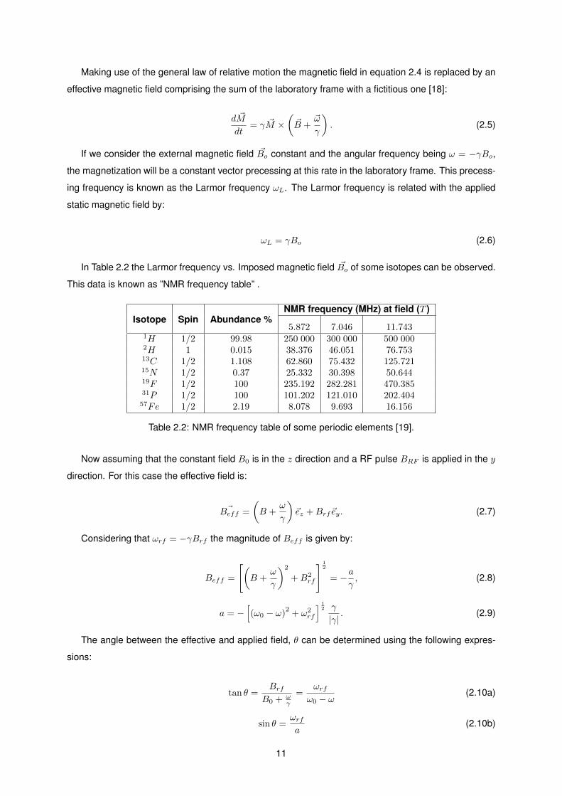
Table 2.2: NMR frequency table of some periodic elements [19].

Now assuming that the constant field B0 is in the z direction and a RF pulse BRF is applied in the y

direction. For this case the effective field is:

~Beff =

(B +

ω

γ

)~ez +Brf~ey. (2.7)

Considering that ωrf = −γBrf the magnitude of Beff is given by:

Beff =

[(B +

ω

γ

)2

+B2rf

] 12

= −a

γ, (2.8)

a = −[(ω0 − ω)

2+ ω2

rf

] 12 γ

|γ|. (2.9)

The angle between the effective and applied field, θ can be determined using the following expres-

sions:

tan θ =Brf

B0 +ωγ

=ωrf

ω0 − ω(2.10a)

sin θ =ωrf

a(2.10b)

11

cos θ =ω0 − ω

a(2.10c)

Using this results the flip angle α of the magnetization with respect to B0 can be determined by

assuming that at t = 0 they are aligned:

cosα = cos2 θ sin2 θ cos at = 1− 2 sin2 θ sin21

2at (2.11)

The flip angle α defines the duration of the RF pulse. A π/2 pulse flips the magnetization by 90

degrees.

2.3 Resonance condition

Analysing the previous expressions that characterize the flip angle α and the angle between the effec-

tive and applied magnetic field θ one can conclude that only when |ω − ωo| ≈ |ωrf | these angles have

significant values. These condition is known as the resonance condition. In NMR experiments, π/2 RF

pulses in resonance with the Larmor frequency are applied to the sample in order to flip the magneti-

zation 90 degrees. Despite of the magnitude of Brf being much smaller than the ~Bo magnitude, it is

enough to cause the desired flip. The previous flip angle equation 2.11 can be reduced to the following

for a resonance pulse:

α = −γBrf tpulse (2.12)

with tpulse being the pulse length. The reasoning using equation 2.4 is only valid for a pulse length

much smaller than the time characterizing the relaxation of the magnetization back to its equilibrium

position. The relaxation concept is crucial in NMR experiments and will be presented next.

2.4 Relaxation and the complete Bloch equations

The interactions between nuclei and the fields created by thermal agitation, even if a lot weaker when

compared to the external field, become very important over long periods of time because of their cumu-

lative effects. In equation 2.4 thermal agitation, interaction between neighbouring nuclei as well as the

influence of fields produced by the electrons in the sample are neglected. These factors influence the

orientation of the magnetization vector and should be taken into account.

We start to assume at equilibrium that the static magnetic field and sample magnetization are both

along the z-axis: ~B = Bo ~ez , ~M = Mo ~ez. When a perturbation, such as a π/2 RF pulse, is applied, the

magnetization starts to re-establishes its initial value along the applied external magnetic field ~B = Bo ~ez

in a process known as relaxation. This decay towards equilibrium is exponential and is expressed by an

12

additional term on each of the components of equation 2.4:

dMz(t)

dt= [ ~M × γ ~B]x − Mz(t)−Mo

T1(2.13a)

dMy(t)

dt= [ ~M × γ ~B]y −

Mx(t)

T2(2.13b)

dMx(t)

dt= [ ~M × γ ~B]z −

My(t)

T2(2.13c)

The time constants T1 and T2 are related to the realignment of nuclei magnetizations with the external

field and are known as relaxation rates. Nuclear magnetic resonance experiments are precisely used to

acquire this frequency dependent relaxation constants.

The spin-lattice relaxation time, T1 is the time constant for the physical processes responsible for the

relaxation of the components of the nuclear spin magnetization vector ~M parallel to the external mag-

netic field, ~Bo (z component, also named longitudinal component). Values of T1 range from milliseconds

to several seconds [9]. Spin-spin relaxation, T2 is at its most fundamental level the evolution time to-

wards the de-coherence of the transverse nuclear spin magnetization. Fluctuations of the local magnetic

field lead to random variations in the instantaneous NMR precession frequency of different spins. As a

result, the initial phase coherence of the nuclear spins is lost, until eventually the phases are disordered

and there is no net xy magnetization.

The equipment proposed in this document, will only measure spin-lattice relaxation time, T1.

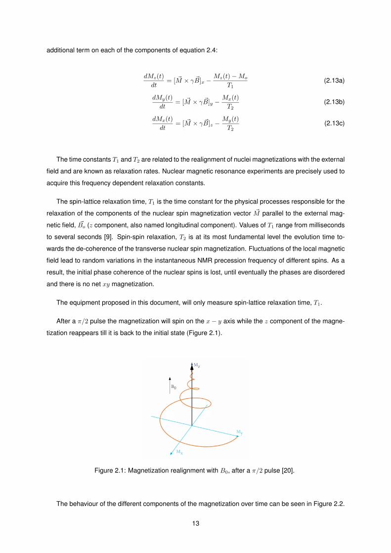
After a π/2 pulse the magnetization will spin on the x− y axis while the z component of the magne-

tization reappears till it is back to the initial state (Figure 2.1).

Figure 2.1: Magnetization realignment with B0, after a π/2 pulse [20].

The behaviour of the different components of the magnetization over time can be seen in Figure 2.2.

13

Figure 2.2: Time evolution of the longitudinal a) and transverse b) components of the magnetizationafter the application of a radio-frequency pulse [21].

2.5 Spin-lattice relaxation time, T1

T1 quantifies the rate of transfer of energy from the nuclear spin system to the environment (the lattice).

There are different relaxation mechanisms and any process that induces magnetic field fluctuations can

be considered one. Every given relaxation process can be defined individually as :

1

T1= E2

c f(τi) (2.14)

where Ec is the intensity of the relaxation mechanism and τi the correlation times of the mecha-

nism [22]. The main relaxation mechanisms are the dipole-dipole relaxation and quadrupole relaxation.

There are other mechanisms, like chemical shift anisotropy, spin rotation and scalar relaxation that are

negligible in 1H FFC experiments.

2.5.1 Relaxation methods

Dipole-dipole relaxation

The dipole relaxation occurs by coupling between two spins and when close to each other experience

each other’s magnetic field. This leads to a slightly different effective magnetic field Beff at one spin that

depends on the orientation of both magnetic dipoles. This is the direct interaction and named the dipole-

dipole interaction. It can also be mediated through chemical bonds which is called J-couplings or indirect

dipole-dipole coupling. Roughly speaking, it arises from hyperfine interactions between the nuclei and

local electrons. The direct dipole-dipole coupling interaction is very large and depends mainly on the

distance between nuclei and the angular relationship between the magnetic field and the internuclear

vectors.

As the molecule vibrates the dipole-dipole coupling is constantly changing as the vector relationship

changes. This creates a fluctuating magnetic field at each nucleus. To the extent that these fluctuations

occur at the Larmor precession frequency, they can cause nuclear relaxation. Since the proton has

the highest magnetic dipole of common nuclei, it is the most effective nucleus for causing dipole-dipole

relaxation [23]. The range of T1 for this relaxation mechanism is between 1 ms - 100 s and its intensity

14

is given, by [22]:

Ec = γSγIh

2πr3(2.15)

Where γi are the gyromagnetic ratios of the nuclei species involved in the relaxation and r the inter-

nuclear distance. If considering equal spins, this process is responsible for a relaxation rate, R1(= T−11 ):

R1 =(µo

4π

)2 3

2γ4I~2I(I + 1)[J1(ωI) + J2(2ωI)] (2.16)

Where I is the spin, Ji(ω) the spectral density functions [14]. This functions are the Fourier transforms of

the correlation functions, Ki(τ) and can be expressed in terms of the correlation time of the dipole-dipole

interaction, τc:

Ki(τ) = Ki(0)e−|τ |/τc (2.17)

The Hamiltonian of the dipole-dipole interaction is dependent on the angle that the inter-nuclear distance

~r, makes with the external magnetic field. Due to particle motion, there is a time dependence on the

angle that provides the function of the correlation time.

The Hamiltonian of this coupling can be described using second order spherical harmonics Y2,m(θ, φ)

with m = 0,±1,±2, expressed by:

Y2,0(t) =

√5

16π[3cos2θ(t)− 1] (2.18)

Y2,1(t) = −√

15

8πsinθ(t)cosθ(t)eiφ(t) (2.19)

Y2,2(t) =

√15

32πsin2θ(t)e2iφ(t) (2.20)

The azimuthal and polar angles φ(t) and θ(t), respectively, describe the instantaneous orientation of the

coupling tensor relative to the magnetic field. The spherical harmonics relate to the correlation functions

Ki(τ), by:

Ki(τ) = Y2,m(t)Y2,−m(t+ τ) (2.21)

Where Y2,−m(t) is the complex conjugate of Y2,m. Considering the fact that the spectral density functions

are the Fourier transform of the correlation functions, and that Ki(0) is obtained by integration:

Ki(0) = Y2,i(t)2 = Y 2i =

∫ 2π

0

∫ π

0

Y 22,isinθdθdφ (2.22)

The spectral density functions can now be determined:

Jo(ω) =24

15r6τc

1 + ωτ2c(2.23)

J1(ω) =4

15r6τc

1 + ωτ2c(2.24)

J2(ω) =16

15r6τc

1 + ωτ2c(2.25)

Together with the expression of the relaxation rate, results in the relaxation rate associated with

15

rotational motion, for isotropic rotational diffusion of molecules and intra-molecular interaction of two-

spin 1/2 systems with fixed inter-nuclear distances, which is known as the BPP model [24].

R1rot =(µo

4π

)2 2γ4I~2I(I + 1)

5r6

[τc

1 + ω2τ2c+

4τc1 + 4ω2τ2c

](2.26)

Quadrupole relaxation

Quadrupole relaxation mechanism relates only to nuclei with spin I > 1/2 and that are not at the center

of tetrahedral or octahedral symmetry, since it will average out its contributions. This mechanism relates

the electric field gradient at the nucleus and the spin. The electric field gradient is responsible for a

torque on the quadrupolar nuclei, leading to molecular reorientations that cause ’friction’ between the

nucleus and the surrounding electrons. This effect is quantified on the quadrupole coupling constant

that appears on the intensity of the relaxation mechanism Ec [22]:

Ec =e2qQ

~(2.27)

Where q is the electric field gradient. The effectiveness of this relaxation mechanism is critically depen-

dent on this coupling. The contribution for the spin-lattice relaxation rate is [23] :

R1 =6I + 9

40I3(2I − 1)

(1 +

Ec

3

)E2

c τc (2.28)

The formalism of both dipole and quadrupole mechanism are very similar, leading to similar expres-

sions [18, 25] .

2.5.2 Total relaxation rate

The studies performed in FC NMR refer to nuclei with spin 1/2 (protons), and in some cases spin 1.

The predominant spin-lattice relaxation mechanism of ”like” spins 1/2 is mainly based on dipole-dipole

fluctuations. For spin 1 nuclei, the quadrupole coupling is much more efficient than dipolar interactions

(among spins of the same species) and the relaxation can be considered entirely caused by this mech-

anism, neglecting the influence of the dipolar relaxation. Cross-correlation effects [18] are negligible in

the context of field-cycling relaxometry, and the total spin-lattice relaxation, T1 in multi-spin 1/2 systems

can be represented as the sum of two-spin 1/2 relaxation rates of index i interacting with all the other

spins in pairs. Then the effective spin-lattice relaxation rate of dipolar coupled spins 1/2 [14]:

1

T1=

∑j 6=i

1

T(i,j)1

(2.29)

Where T(i,j)1 is the spin-lattice relaxation time of the specific spin i interacting with all the other spins

in the sample of the multi-spin 1/2 systems [14].

Relaxation mechanisms can be divided into two groups, the intra-molecular and intermolecular mech-

anisms. Quadrupole interaction is exclusively intra-molecular and dipole-dipole interaction can be con-

16

sidered both. Intermolecular dipolar interactions lean to fluctuate much more slowly than intra-molecular

couplings. This occurs because intermolecular dipolar interactions are governed by Brownian motions

of the molecule over distances exceeding the dimension of the same. The spin-lattice relaxation rate

resulting from both contributions may be written as

1

T1=

1

T intra1

+1

T inter1

(2.30)

This is plausible because the two contributions refers to very different time scales. While quadrupole

interaction also exists in different time scales than the previous two contributions, the same argument

can be applied for the total relaxation rate:

1

T1=

1

TDD1

+1

TQP1

(2.31)

2.6 NMR measurements and the Fast Field Cycling Principle

For a typical NMR experiment in order to measure the spin lattice relaxation time T1, an external mag-

netic field ~Bo is applied aligning the sample net magnetization. Followed by a RF pulse, it shifts the net

magnetization 90 degrees which starts realigning with external magnetic field ~Bo immediately after. This

induces a signal known as Free Induction Decay (FID). This FID is the signal induced by the sample

magnetization ~M in the transverse coil (which produces the RF pulse) to the external magnetic field ~Bo.

The RF pulse needs to be at the Larmor frequency and as it can be deduced from equation 2.6 to cause

a 90 degrees shift of the magnetization for a given gyromagnetic ratio.

The evolution of the magnetization component Mz(t) parallel to the applied magnetic field ~Bo de-

pends on its magnitude and is described by the Bloch equations 2.13. For a NMR experiment Mo = Meq

(equilibrium magnetization). The evolution of Mz(t) can be rewritten as:

dMz

dt= − 1

T1(Bo)[Mz(t)−M(eq)(Bo)] (2.32)

In a typical field cycling NMR experiment the sample is initially placed in a magnetic field BoP , where

it is polarized for a time ∆tp. Following this, the magnetic field is switched down to a lower field value BoE ,

for a time ∆tE . The goal is to polarize the sample as much as possible in order to let the magnetization

evolve by quickly switching the field from BoP to BoE (tswitching T1(BoE)). After a certain evolution

time ∆tE a new field known as the detection field BoD is applied that can have the same magnitude of

the polarization field (BoD = BoP ). A typical cycle of this technique can be observed in Figure 2.3.

In a) the variation of the applied magnetic field ~Bo is exemplified. The transitions between different

values of ~Bo must be fast but not to fast. This conditions arise from the fact that the correct requirement

for an ideal cycle is ’reversibility’. In the limit te → 0 and BoP = BoD the magnetization of the sample

in the end of the polarization phase should be replicated as the initial magnetization in the detection

phase without any entropy increment in the sample material. This is achieved by making the field tran-

sition on one hand so fast that the relaxation mechanisms are negligible (no energy transfer between

17

Figure 2.3: Typical FFC NMR cycle [1].

atoms/molecules during the transition) and on the other hand slow enough in comparison with the Lar-

mor velocity preserving the angle between ~M(t) and ~Bo(t) (known as adiabatic transition). This fast,

yet adiabatic cycle completely eliminates possible unpleasant effects arising from equation 2.32 and is

translated by the following condition [9]:

| ~Bo × d ~Bo

dt |B2

o

γBo (2.33)

In b) the sample z-component of the magnetization under the influence of a) can be observed. The

magnetization evolves according to each applied field exponentially as expected. Between t5 − δ and t5

the net magnetization drops to zero due to the RF pulse followed by its relaxation. In Table 2.3 we can

see the equation that defines the magnetization on each phase of the cycle.

In c) we can observe the magnetic impulse B1(t) that is obtained through the RF coil. This pulse has

a frequency ωo in resonance with the Larmor frequency and has a duration of δ (typically in the order of

18

Polarization (P) Mz(t) = MeqD + (MeqP −MeqD)(1−exp[−t/T1P ])Transition (P → E) Mz(t) = Mz(tP ) = MeqP =const

Evolution (E) Mz(t) = MeqP + (MeqP −MeqE)(1−exp[−t/T1])Transition (E → D) Mz(t) = Mz(tE) =const

Detection(D) Mz(t) = Mz(tE) + (MeqD −Mz(tE))(1−exp[−t/T1D])

Table 2.3: Mz(t) for each part of the FFC cycle [9].

10−6 s). Figure 2.3 d) is the NMR detected signal, Free Induction Decay (FID), which corresponds to the

evolution of the x− y components of the magnetization vector. Ideally the FID signal would be detected

in the end of the evolution phase ( ~BoE) in order to measure T1(BoE). However the detected signal has

a Signal to Noise ratio associated given by [14] :

S/N ∝ B3/2o (2.34)

Given the proportionality with B3/2o it is desirable to detect the FID signal for the highest applied field

possible.

The detected field is only performed after the transition BoE → BoD at t = t5. In this instant the

magnetization is given by [1]:

Mz(t5) = MD

[1− exp

(−t5 + δ

T1(BoD)

)]+ [∆MZon +Mz(t3)]exp

((−t5 + δ)

T1(BoD)

)(2.35)

Considering that:

β = exp

[−t5 + δ

T1(BoD)

](2.36)

The expression 2.35 becomes:

Mz(t5) = βMz(t3) + β∆MZon +MD − βMD (2.37)

If we can make sure MD, β and ∆MZon are constant for a NMR experiment, equation 2.37 becomes:

Mz(t5) = βMz(t3) + const. (2.38)

This relation allows for the magnetization in t5 to be proportional to the magnetization in t3 making

possible the measurement of T1(BoE) with a much higher signal to noise ratio.

19

2.7 Limitations of the technique

In order to achieve quality measurements the polarization and detection fields need to be as high as

possible, appropriate switching times to the given system under study and precise and stable applied

fields. Thermal stability is also required for a precise measurement of T1. Field stability is usually

assured, but extra considerations are necessary for low fields, such as possible external local magnetic

fields and earth magnetic field.

2.7.1 Signal to Noise ratio

The signal to noise ratio is an important aspect of NMR measurements and can be a crucial limitation.

When the detection field is repeated in subsequent cycles accurately enough sensitive detection is

possible, so the signals can be accumulated. Equation 2.34 tells us that the Signal to Noise ratio

is proportional to B3/2o but other quantities are also relevant. For FFC NMR experiments where the

polarization and detection fields may have different magnitudes the S/N ratio is given by the following:

S/N ∝ BoP ξ

√ηQVs

kBT

( νd∆ν

)(2.39)

Where η is the RF coil filling factor (Sample Volume/Coil Volume), Q the quality factor of the RF

coil, Vs the sample volume, kb the Boltzmann constant, T the absolute temperature, νd is the detection

Larmor frequency, ∆ν the bandwidth of the signal receiver and ξ the reciprocal noise level of the receiver.

While high polarization and detection fields are crucial for a good sensitivity and signal acquisition the

consideration of other factors can also increase the S/N ratio.

2.7.2 Field Cycling and Fast Field Cycling

The field switching can be performed in two ways: mechanically or electronically. Electronic switching

means changing in the magnetic field without moving the sample. In mechanical switching the sample

is physically moved from one place to another, where two different magnetic fields exist.

By moving the sample undesired effects might arise (specially in liquid samples), the temperature

control becomes difficult to perform, and field switching can only be performed as fast as ≈ 50 ms.

Electronic field variations by changing the current applied to the main coils can perform switching as

fast as 1 ms and have a accurate sample temperature control. Mechanical switching is known as Field

Cycling and electronic switching as Fast field Cycling. The proposed equipment will perform electronic

field variations.

20

2.8 Competing techniques

2.8.1 Inversion-recovery

Inversion-recovery is a technique used to acquire relaxation times worth mentioning. It consists in the

application of a π pulse, into a magnetized sample, which inverts the magnetization. After a variable

delay τ , a π/2 pulse follows, flipping the magnetization into the xy plane. An example can be observed,

for a arbitrary time τ1, in the following figure:

Figure 2.4: Magnetization in a typical Inversion-recovery experiment [22].

Depending on τ , the magnetization can assume any value between | ~M(t)| < Mo. This is responsible

for a signal intensity, proportional to the magnetization magnitude, for each value of τ .

Inversion-recovery occurs at a single Larmor frequency, or fixed magnetic field ~Bo and rely on RF

pulses , ~B1. The inversion-recovery can only be applied to Larmor frequencies typically above 5 MHz.

The reason for this arises from the relation between signal to noise ratio and the applied magnetic field

(equation 2.34). Given the description of the technique, and that the FFC NMR relaxometer has all

the necessary technical characteristics it is possible to perform Inversion-recovery with the proposed

equipment.

2.8.2 T1ρ relaxometry

There are different techniques able to measure the same physical quantities that FFC does, but there

is only one which operates inside the frequency range [10kHz; 20MHz], the so called T1ρ relaxometry.

T1ρ is the spin-lattice relaxation in the rotating frame, and is the physical quantity measured with this

technique. It is possible to relate T1ρ with T1 and T2 by applying a spin-locking frequency pulse, B1. By

forcing ω1 tend to zero, T1ρ approaches T2 and when ω1 approaches the Larmor precession frequency

ωL , T1ρ approaches T1, i.e T1ρ ≈ T1. The relation between T1ρ with T1 and T2 makes the measurement

of this physical constant a parallel technique to FFC.

This technique allows to study the spin relaxation process in the frequency range of [10−30] kHz, and

is used for very small Larmor frequencies, which corresponds to fields smaller than earth field. In this

case the signal to noise ratio is very poor (equation 2.34) in most relaxometers, making this technique

useful in this domain.

21

2.9 Physical Models

Given the interest in simulate and evaluate physical quantities in order to achieve a reliable electromag-

net, different physical phenomena need to be defined and modelled.

The first and most important physical phenomena in the development of the magnetic core is elec-

tromagnetism. The coils will be excited by an electrical current leading to the creation of a magnetic field

which is described by the following Maxwell equation that couples both ~B, the free current density ~Je

and the electric field:

∇× ~B = µo

(~Je + εo

∂ ~E

∂t

)(2.40)

Where µ stands for the magnetic permeability of the material. The magnetic field in the electromagnet

is specified through equation ??, but since the magnetic flux makes a transition to the air the following

Maxwell equation is required to compute the magnetic field in the air:

∇. ~B = 0 (2.41)

A software simulation is used to perform the computations where large and complex problems are

solved. The introduction of the vector potential ~A can reduce the computational resources required. The

relation between ~A and the magnetic field ~B is given by:

~B = ∇× ~A (2.42)

Another important phenomena are the heating of the coils and the heat transfer between different

materials and air.

The heating of the coils occurs through electrical resistance of the cooper wire to the imposed current

and the dissipated power is given by:

P = RI2 (2.43)

The heat transfer then occurs from the coils to air and the electromagnet (iron). The general heat

equation is given by:

∂~u

∂t− α∇2~u = 0 (2.44)

where α is a positive constant and ∇ the Laplace operator. In the physical problem of the heat

transfer, u(x, y, z, t) is the temperature and α the thermal diffusivity. This equation is given by the first law

of thermodynamics (energy conservation) and can be rewritten assuming no mass transfer or radiation:

ρcp∂T

∂t−∇.(k∇T ) = Q (2.45)

where ρ is the mass density of the material, cp the specific heat capacity and Q the volumetric heat

22

source [W/m2]. Both equations 2.43 and 2.45 define the heat source and heat transfer phenomena of

the electromagnet.

Finally, the air flow phenomena is necessary given the requirement of air cooling of the electromag-

net. The equations that govern the motion of fluids are the Navier-Stokes equations. If considering a

compressible Newtonian fluid, The Navier-Stokes equations can be expressed as:

ρ(∂~u∂t

+ ~u.∇~u)= −∇p+∇.

[µ(∇~u+ (∇~u)T )

]− 2

3µ((∇.~u)I

)+ ~F (2.46)

where ~u stands for the velocity of the fluid, p its pressure and µ the dynamic viscosity, I the iden-

tity matrix and ~F the applied external forces. The Navier-Stokes equations define the conservation of

momentum and the continuity equation is required for the conservation of mass:

∂ρ

∂t+∇.(ρ~u) = 0 (2.47)

23

24

Chapter 3

Electromagnet: Design and Numerical

Simulation

3.1 Electromagnet and Coils

The main component of the FFC equipment is the electromagnet. The electromagnet is the support for

the main coils, provides a path for the magnetic field flux and also allows for the sample insertion. Iron

have a permeability in the order of 1050 compared with just 1 for air. This means that a iron core can

carry a magnetic flux 1050 times higher than that of air. However, when a magnetic flux flows in a such

a electromagnet, two types of undesired effects occur. One known as eddy currents and the other as

hysteresis effects.

Hysteresis effects

Hysteresis is the lagging of the magnetization of a ferromagnetic material, such as iron, behind variations

of the magnetizing field. When ferromagnetic materials are placed within a coil of wire carrying an

electric current, the magnetizing field, or magnetic field strength ~H , caused by the current forces some

or all of the atomic magnets in the material to align with the field. The net effect of this alignment is

to increase the total magnetic field, or magnetic flux density ~B . The aligning process does not occur

simultaneously or in step with the magnetizing field but lags behind it.

If the intensity of the magnetizing field is gradually increased, the magnetic flux density ~H rises to

a maximum, or saturation, value at which all of the atomic magnets are aligned in the same direction.

When the magnetizing field is diminished, the magnetic flux density decreases, again lagging behind

the change in field strength ~H . In fact, when ~H has decreased to zero, ~B still has a positive value

called the remanence or residual induction, which has a high value for permanent magnets. ~B itself

does not become zero until ~H has reached a negative value. The value of ~H for which ~B is zero is

called the coercive force. A further increase in ~H (in the negative direction) causes the flux density to

reverse and finally to reach saturation again, when all the atomic magnets are completely aligned in the

25

opposite direction. The cycle may be continued so that the graph of the flux density lagging behind the

field strength appears as a complete loop, known as a hysteresis loop. The energy lost as heat, which

is known as the hysteresis loss, in reversing the magnetization of the material is proportional to the area

of the hysteresis loop. Excessive heat loss can overtime shorten the life of the insulating materials used

in the manufacture of the windings and structures.

The memory effect can affect the desired magnetic field magnitude and is overcome by designing

the auxiliary coils. The auxiliary coils are supplied with an opposite current compared to the main coils

current. This eliminates the remaining magnetic field inherited. The heating effects will be balanced by

a cooling system.

Eddy Current losses

Eddy Current Losses on the other hand are caused by the circulating currents induced into the iron

caused by the variation of the magnetic flux around the electromagnet. These circulating currents are

generated because for the magnetic flux the electromagnet acts like a single loop of wire. Since the iron

electromagnet acts like a conductor, the eddy currents induced will be significant. Eddy currents oppose

the flow of the induced current by acting like a negative force generating resistive heating and power

loss within the electromagnet.

Eddy current losses within a iron core can not be eliminated completely, but they can be greatly

reduced by reducing the thickness of the iron core. Instead of having one big solid iron core as the elec-

tromagnet, the magnetic path is split up into many thin pressed iron plates known as laminations. The

thin strips of insulated metal are brought together to produce a solid laminated core. These laminations

are insulated from each other by a coat of varnish in order to increase the effective resistivity of the

core, thereby increasing the overall resistance limiting the flow of the eddy currents. The result of this

insulation is that the undesired induced eddy current power-loss in the core is greatly reduced (Figure

3.1). This will be considered in the development of the ferromagnetic core. The losses of energy, which

appears as heat due both to hysteresis and to eddy currents in the magnetic path, is known commonly

as transformer core losses.

Figure 3.1: Effect of laminations in the eddy currents.

26

Electromagnet geometry

The electromagnet geometry will be based on the previous equipments developed in IST [1, 12]. This

geometry is composed by ”E” shaped plates. This plates are known as Transformer E-shaped plates

and are made of iron. They have standard measurements as exemplified in Figure 3.2.

27

Figure 3.2: Standard proportions of Transformer E-shaped plates, designed in AutoCAD R© 2015.

These are the standard proportions of the E-shaped plates. There are different values of b available in

the market. The FFC NMR equipments developed in IST rely on b = 18 cm plates [1]. The electromagnet

consists on two of the E’s brought together with a slight cut on each of the middle feet where the sample

will be accommodate Figure 3.3.

Figure 3.3: Electromagnet consisting in two E-shaped plates.

28

A symmetrical field and symmetrical coils are desired, so the height of the electromagnet must equal

to helectromagnet = b/3 in order to have a squared section in the middle foot. An example can be seen in

Figure 3.4

Figure 3.4: Side view of pilled E-plates with height h = b/3, the axis scale is presented in cm. Designedin COMSOL Multiphysics R© 4.3 .

Coils

The coils, when applied with a specific voltage allow for creation of the magnetic field. Coils will be

inserted around the middle feet. The maximum height of each coil must be less than the available space

for the sample in order to insert and remove them in case of a maintenance is required. The maximum

width of each coil is also limited by the width between the middle and external foot. There is also a limit

for the number of coils allowed in the ferromagnetic electromagnet and a certain distance should be kept

between the sample site and the first coil for field uniformity as well as a gap between different coils in

order to allow for more efficient air cooling.

3.2 Simulation: COMSOL Multiphysics R©

In order to define the parameters of the electromagnet, a simulation is performed using COMSOL

Multiphysics R©.

COMSOL Multiphysics R© is a general-purpose software platform, based on advanced numerical

methods, for modelling and simulating physics-based problems. COMSOL Multiphysics R©, allows to

account for coupled or multi-physics phenomena. The main purpose is to visualize and analyse the

magnetic field in the sample site but other phenomena will be observed such as Joule heating and

cooling requirements.

Before the simulation is performed it is important to understand and compile the physical quantities

that are susceptible to change and understand their influence in the characteristics of the spectrometer:

29

• Electromagnet size: Different E-shaped transformer plates are available with different b sizes,

which is directly related with the electromagnet size and volume. The size of the electromagnet

influence the magnetic flux density and maximum magnetic field. On one hand the smaller the

electromagnet is the higher is the possible magnetic field, on the other hand the smaller is the

available space for the coils limiting the number of turns and therefore the magnetic field.

• Sample gap size: This gap needs to the removed from the E-shaped plates. The smaller the gap

the higher will be the magnetic field magnitude at the sample site but the smaller the height of the

coils will be since they are inserted through the gap. There is a minimum limit since the sample

need to be heated with air and the RF coil needs to involve the sample.

• Maximum current applied to the coils: The magnetic field at sample site is directly related with

the applied current. The current power supply is able to operate between 0 − 5 A. Joule heating

effects must be considered as well as the fact that a better performance from the power supply is

observed for currents below 4.5 A.

• Number of coils: Different sets of coils will be used since each coil has a maximum height of the

sample gap. The more coil sets the electromagnet has the higher will be the magnetic field but the

other limitations might arise such as cooling ability and space.

• Number of turns in each coil: This number should be as high as possible since it is directly

related with magnetic field magnitude. It is limited by the gap size, length between E-plate feet,

Joule loss effects and wire cross section.

Other parameters are of importance but a starting point is required. The starting point is the magnetic

field and only then the other parameters are adjusted. The possible range of values of the previous

mentioned quantities can be observed in Table 3.1.

E-plate standard size (b) 12/13.5/15 [cm]Number of coils 2 - 8

Number of turns per coil [50− 300]Max. current in coils [0− 5] [A]Minimum gap size 15 [mm]

Table 3.1: Possible range of values for the simulation.

The minimum gap size arises from specifications of the sample requirements and the minimum radius

of glass tubes available for the sample heating system. Further explanation of this system is given in

Chapter 5.

3.2.1 Geometry and material definition

The first step for the simulation was the definition of the geometry as well as the materials. The geometry

consists on the electromagnet, coils and air box in the sample site, where the magnetic field will be

evaluated. The electromagnet geometry was defined in terms of the variable b in order to perform a

parameter sweep to evaluate the best geometry. This is described in Figure 3.5

30

Figure 3.5: Core design depending on the b variable.

The electromagnet is first defined in a 2D plane using the ”Work Plane” command. A rectangle is

created (r1) with a width b and height 2b/3 then three other rectangles are created (r2 , r3 and r4) that

are subtracted to the first using the command ”Boolean operations → Difference” in order to create

the first E-shaped Plate (sample site already included). The second plate is created similarly and are

distinguished by ”Up” and ”Down” in Figure 3.5.

Being the electromagnet defined in 2D the third dimension is added using the command ”Extrude”

which simply gives height to the object created in the ”Work Plane”. In order to have a square geom-

etry in the sample site as mentioned in section 3.1, the height is defined as b/3 resulting in the final

electromagnet geometry.

Figure 3.6: Final Core geometry. The axis scale is presented in cm.

31

Notice that the electromagnet is not laminated into thin plates, as it will be necessary to avoid eddy

currents losses ( Section 3.1). The reason for this arises from the fact that such phenomena is already

well studied and efficient solutions are known making unnecessary the need of using computational

resources that will be needed in latter stages of the simulation. A better homogeneity might be observed

in the simulation compared to the real case for this reason.

The coils follows a similar process with some dimensional limitations that need to be respected.

These limitations are: the coil height needs to be smaller than the sample gap size and must fit inside

the inner feet within the outer feet (Figure 3.7).

Figure 3.7: Coil dimensional limitations. The axis scale is presented in cm.

An inner square with length b/3 and an outer square of length 2b/3 − b/12 is created in a 2D plane

parallel to the previous using ”Work Plane” command. ”Boolean operations → Difference” is used to

create the 2D coil and the ”Extrude” command to create the three dimensional shape. This is replicated

several times in order to have all the coils. Two additional coils are designed that compensate perma-

nent fields in the electromagnet or the earth magnetic field. Similar to the main coils, but with smaller

dimensions.

A block is created with 15 mm height (equal to the sample gap size), width and length of 2b/3− b/12

centered in the middle of the gap and finally an air sphere containing the whole geometry of radius b is

defined (made invisible). The final geometric result can be observed in Figure 3.8.

After the geometry, material definition follows. Three materials are used: air, copper and iron. The

electromagnet was defined as iron, the coils as copper, the air block (blk1) and sphere as air (Figure

3.8). Each material requires physical parameters to be defined. Three parameters for each material are

required at this stage : relative permeability µo, relative permittivity εo and electrical conductivity σ [S/m].

The air is define to have an electrical conductivity σ of 3 [S/m] in order to facilitate the convergence of

computation and does not influence the simulation results.

32

Figure 3.8: Final geometry with material properties and definition. The axis scale is presented in cm.

3.2.2 Magnetic field Simulation

In order to observe to magnetic field the module ”Magnetic Field (mf)” is added as well as a ”Stationary

study”. The FFC cycle won’t be computed yet since the goal is to observe the maximum possible

magnetic field at sample site for a given current Icoil applied to each main coil. The ”Stationary study”

computes all the variables until it finds a stationary solution, which is suitable for now.

We begin by defining a coil using the command ”Magnetic Field → Multi-Turn Coil Domain”. Several

parameters need to be defined such as: the relation by which the magnetic field is calculated, the

material type of the coil, the type of coil, coil conductivity, number of turns, coil wire cross-section area

and how the coil is excited (Figure 3.9). The coil type is chosen to be circular which isn’t entirely correct

but is corrected by the ”Reference Edge” command. This command allows to choose a geometry for the

path in which the current flows. The path chosen were the coil edges, which is in conformity with the

problem. The number of turns is defined as the variable ”N ”. The type of coil excitation can be through

voltage or through current. The power supply available does so by current [1] and its value defined as

the variable Icoil. The wire cross-section area depends on the maximum current applied, and will be

specified later.

Finite element method and Mesh definition

COMSOL Multiphysics R© relies on the ”Finite element method” (FEM) to solve physical problems. The

Finite element method is common in solving engineering problems such as heat transfer, fluid flow and

electromagnetic fields.

The analytical solution of such problems usually requires the solution of boundary value problems

for partial differential equations. The method yields approximate values of the unknown variables at a

discrete number of points over the domain, which in this particular software is called ”Mesh”. In order to

solve a problem, it divides the whole into smaller, simpler parts known as finite elements. The simpler

equations modelling these finite elements are them assembled into larger matrices that model the entire

problem. After this, the FEM uses variational methods to approximate a solution by minimizing an

33

Figure 3.9: Magnetic field and Coil definition.

associated error function. For the creation of the mesh two important parameters need to be defined:

Maximum element size, and minimum element size. Two different meshes will be created, one for the air

box in the sample site, and another for the rest of the geometry. The reason for this arises from the fact

that a more detailed resolution in the magnetic field of the sample site is desired, hence a more detailed

mesh.

The sizes of the parameters of each mesh can be seen in the Figure 3.10. The problem is now fully

defined.

Parameter sweeping

The problem is defined and the variables require definition. Four parameters matter in order to define

the simulation: Maximum current applied to the coils, number of coils, number of turns per coil and the

E-shaped plates size defined by b. They all influence each other. A certain maximum current requires a

certain coil wire cross-section area, which will limit the number of coils since of size limitation imposed

by b. The number of coils is also limited by b which influences the number of turns in the electromagnet.

All the length quantities will be expressed in mm. The first parameter to consider is the number of

coils in the electromagnet. In order to obtain an expression that allows to calculate this parameter the

following considerations should be taken into account:

• The available space in each feet is b/2− 7.5 mm (given the gap is 15 mm)

• 5 mm must be left between the sample site and the first coil (homogeneity purposes)

• Each coil has a final height of around 14 mm (coil + casing)

34

Figure 3.10: Mesh parameters of the sample site air box and the rest of the geometry (left) Visual detailof the mesh (right) .

• In between coils a 2.5 mm gap is required for air circulation which allows cooling

• 5 mm are necessary for the auxiliary coil

Having this in consideration the resulting expression is the following:

NC(b) = (b− 3.5)/1.65 (3.1)

The number of coils corresponds to the result rounded to the even lower integer, Ncoils.

As we’ve seen in Table 3.1 the maximum current is between ]0− 5] A .

Applying 5 A to the main coils results in a higher maximum magnetic field but also higher power

consumption and Joule losses since the heating power is proportional to the product of the resistance

and the square of the current as mentioned in section 2.9. Being this the case two possible currents are

considered, 3 A and 5 A.

According to the manufacturer a current of 3 A requires a 0.9 mm diameter circular wire (in order to

avoid damage by overheating) and a current of 5 A requires a 1.1 mm diameter wire. Some technical

aspects of the coil construction were also acquired that must be accounted for: the wire is coated with a

special insulator in order to avoid short circuit and the winding technique has some properties. A circular

wire of 0.9 mm diameter ends up with a 1.02 mm (D3A) diameter with the coat, and the 1.1 mm wire with

1.28 mm (D5A) diameter. This reduces the available space and hence the number of turns.

The coils are composed by several layers. The winding technique consists in odd layers having n

turns, the even layers n− 1 turns while the last layer always has n− 1 turns. The coil height is fixed to 14

mm, in order to fit properly inside the gap and allow some extra space for looseness. The width of each

coil is defined by the following expression:

w = b/6− 3[mm] (3.2)

35

Figure 3.11: Coil winding technique used in the current project.

Some looseness is desired as well, and 3 mm are considered for each side . Given the details of

the winding technique and the fact that 1 mm of thermal tape are required on each side of the coils the

number of turns per layer (NTL) alternates between 1.2/D and (1.2/D)− 1.

The number of layers (NL) is simply given by w/D (coil coating considered) and the number of turns

per coil is given by the expression:

NT =

NTL × (NL − 1)/2 + (NTL − 1)× (NL + 1)/2, if NL is odd

NTL × (NL)/2 + (NTL − 1)× (NL)/2, if NL is even(3.3)

With this data the number of coils, maximum number of turns of each coil can be calculated for a given

current and b.

All this information is compiled in Table 3.2 for different values of b.

It is desired to reduced the size of the electromagnet compared to the previous versions and for this

reason the b = 18 cm wasn’t considered.

36

bN

coils

Coi

lWid

thcm

(w)

Max

.cu

rren

tIcoil[A

]W

iredi

amet

erD

[mm]

Ntu

rns

perl

ayer

sN

TL

Nla

yers

NL

Ntu

rns

perc

oilN

T

31.02

1217

114

124

1.7

51.28

913

110

31.02

1219

218

13.5

61.9

51.28

915

127

31.02

1217

161

156

2.2

51.28

917

144

Tabl

e3.

2:P

aram

eter

swee

ping

37

Magnetic field - Results

The parameters are now defined for each case of Table 3.2 and a ”Stationary Study” can be computed.

Different plots are created to evaluate the magnetic field. A standard example of the observations can

be made in Figure 3.12.

Figure 3.12: Magnetic field plots: Volume and Arrow line.

The magnetic flux vector can be observed as well as the density plot. Higher density can be observed

in the inner corners, and the opposite in the outer corners. The arrow surface shows the path and

direction of the magnetic flux lines along the electromagnet and the fringing effect is seen in the outer

area of sample site. The differences in the magnetic flux density, and its direction are all expected effects

that confirm the accuracy of the simulation interpreting the problem.

A more detailed view of the density of the magnetic flux can be seen in Figure 3.13.

38

Figure 3.13: Magnetic field plots: Volume, Contour and Arrow line.

The magnetic flux is almost negligible in the outer corners since this areas would represent a longer

path for the flux lines. A plot of the fields line can be observed in Figure 3.14 for a more detailed view of

the fringing effect and field lines path. The fringing effect, although significant doesn’t seem to affect the

field uniformity in the middle of the sample site.

Further evaluation is necessary and a plot of the magnetic field in the sample site is desired to

evaluate the maximum magnetic field available to the NMR studies. This is achieved by creating a

parallel plane to the section surface.

The simulation is performed for all cases of Table 3.2 in order to evaluate the magnetic field obtained

in the sample site.

In Table 3.3 the results are presented as well as a comparison with the previously built electromagnet

[1].

The electromagnet volume is by the following equation:

V (b) =b2

3× (b− 1.5)cm3 (3.4)

39

Figure 3.14: Magnetic field plots: Volume and Streamline.

Where Vo corresponds to the volume of a b = 18 cm electromagnet, Vo = V (18) cm3. The weight is

calculated by:

W (V ) = V (b)× 10−6 × ρiron (3.5)

Where ρiron stands for the iron volumetric density, ρiron = 7870 [m3/Kg]. The wire length (l) is

obtained by considering the average length of a turn equal to b/2 × 4. The coil resistance is calculated

with the expression:

R = ρl

A(3.6)

Where ρ represents the electrical resistivity and A the cross section area.

By evaluating all the available cases it was decided to pursue the electromagnet with the character-

istics: b = 13.5 cm and Icoil = 3 A which possesses a maximum sample site magnetic field of 0.329 T .

The decision of pursuing this electromagnet configuration was based on the volume ratio (significant im-

provement in size and portability compared to the previous electromagnets), maximum applied current

(less power consumption) and the cooling requirements being similar to the available FFC equipment.

40

bC

ore

Wei

ght[Kg]

Volu

me

Rat

ioV(b)/Vo

I coil[A

]To

taln

oftu

rns

Wire

leng

th[m

]C

oilR

esis

tanc

e[Ω]

Joul

eLo

sses

[W]

Max

imum

~ Bo[T

]

3780

187.0

4.9

44.5

0.196

123.966

0.283

5440

105.6

1.4

35.0

0.185

31308

353.2

9.3

84.0

0.329

13.5

5.737

0.409

5762

205.7

2.7

67.2

0.310

31518

455.4

12.0

108.3

0.386

157.97

0.568

5864

259.2

3.4

85.2

0.365

1814.024

15

640

230.4

3.2

78.9

0.208

Tabl

e3.

3:C

ore

wei

ght,

volu

me

ratio

and

max

imum

mag

netic

field

fore

ach

confi

gura

tion

41

Equivalent magnetic circuit for sample site magnetic field calculation

The magnetic field of the sample size can also be estimated by establishing the corresponding magnetic

circuit. This is performed in order to verify the conformity of the simulation.

Figure 3.15: a) Top 2D electromagnet view with path length (mm) and b) Magnetic circuit.

In Figure 3.15 the electromagnet ”average” path length is indicated along with the equivalent mag-

netic circuit . By simplifying the circuit an equivalent circuit is obtained:

Figure 3.16: Equivalent magnetic circuit.

The equations to consider are:

Tt = NI = <eqφt (3.7)

φt = BgapSgap (3.8)

42

NI = <eqBgapSgap (3.9)

Bgap =N

<eqSgapIcoil (3.10)

The magnetic field magnitude , according to equation 3.10 is a function of the number of turn (6×218),

the applied current (Icoil), and sample site cross sectional-area (4.5 cm× 4.5 cm) and <eq.

< stands for the reluctance of the circuit which is calculated through the following expression:

< =l

µoµrS(3.11)

Where l is the length of the circuit, S the cross-sectional area, µo and µr the vacuum permeability

and relative permeability of the material, respectively . The equivalent reluctance <eq of the magnetic

circuit is calculated by:

<eq =<eq1

2+ <eq3 + <B1E1

= 6049010H−1 (3.12)

Where:

<eq1 = <AB + <AF + <FE

<eq2 = <BC + <CD + <DE

<eq1 = <eq2

<eq3 = <BB1+ <EE1

The magnetic field in the sample site is proportional to the applied current of the coils:

Bgap ≈ 0.107Icoil (3.13)

For a 3 A current a 0.3217 T magnetic field is expected. This can be considered similar to the result

obtained through the simulation (deviation of 0.3%).

A more detailed study of the magnetic field is desired for better analysis of the field homogeneity.

43

3.2.3 Field Homogeneity

The homogeneity of the magnetic field is given by:

H =∆B

Bo(3.14)

It depends on the variation and the magnitude of the magnetic field in a given volume. The smaller

the variation is, the greater the homogeneity will be.

The homogeneity requirement arises from the fact that the sample needs to be polarized evenly

by the same field magnitude in order for the RF pulse to match the Larmor frequency. This not only

requires a uniform area in the sample site middle plane but also an uniform volume. To further evaluate

this volume, three planes are created: the middle sample site plane (y = 0) and two additional planes in

y = ±0.35 cm .

The magnetic field magnitude in the center of the planes y = ±0.35 cm should match the magnitude

of the middle plane, since the evaluated sample will be in the y range of ]−0.35, 0.35[ cm. Figure 3.17 a)

is a diagonal plot of the sample site section. Despite the divergence in magnetic field values in the limits

of the section in both three planes the magnetic field magnitude converge to the 0.329 T .

Figure 3.17: a) 3D Line Plot of the magnetic field magnitude in the three planes.The axis scale ispresented in m. b) Contour plot for plane y = 0. Designed in COMSOL Multiphysics R© 4.3 and MatLab2015.

44

Figure 3.18: Contour plot for plane: a) y = 0.35 cm and b) y = 0.35 cm.

So one may observe the homogeneity, contour plots of each plane are performed using MatLab.

Two square areas are defined : the inner square (2 cm× 2 cm, Ai) and an outer square (4.5 cm× 4.5

cm, Ao) that corresponds to the middle foot section. For the y = 0 plane (Figure 3.17 b)) the magnetic

field is uniform in the centered square Ai with a magnetic field of 0.3288 T in the central point. The outer

square Ao presents higher non-homogeneity since it is close to the sample site section limit and the

fringing effect starts to become significant.

The same method is applied to the planes y = ±0.35 cm.

In the y = 0.35 cm plane (Figure 3.18 a)) the magnetic field presents a higher uniformity in the

centered square Ai with a magnetic field of 0.3289 T in the central point. The outer square Ao presents

high non-homogeneity as expected.

In the y = −0.35 cm plane (Figure 3.18 b)) the magnetic field is also uniform in the inner square Ai

with a superior uniform contour line than the y = 0 case with a magnetic field of 0.3289 T in the central

point.

In order to evaluate the homogeneity magnitude, 16 points are evaluated on each plane. This points

corresponds to the vertex and middle edges points of the inner and outer square. In Table 3.4 B1 to B3

points correspond to the inner square and B4 to B6 to the outer square points. The homogeneity values

are calculated for each point through equation 3.14 and a mean value is presented for each square.

The magnetic field values in the corners and middle points of the squares are registered to evaluate

the homogeneity. Only a quarter of the values are shown since the sample site possesses magnetic

symmetry both with the xx and zz axis.

45

Inner square (Ai) Outer square (Ao)cm/T B[T] ∆B/Bo % B[T] ∆B/Bo %

B1 0.3276 B4 0.2152y = 0 B2 0.3284 0.22 B5 0.2678 22.94

Bo = 0.3288 B3 0.3282 B6 0.2771B1 0.3289 B4 0.3023

y = 0.35 B2 0.3288 0.01 B5 0.2397 15.29Bo = 0.3289 B3 0.3288 B6 0.2936

B1 0.3289 B4 0.3026y = −0.35 B2 0.3286 0.03 B5 0.2559 13.46Bo = 0.3289 B3 0.3288 B6 0.2951

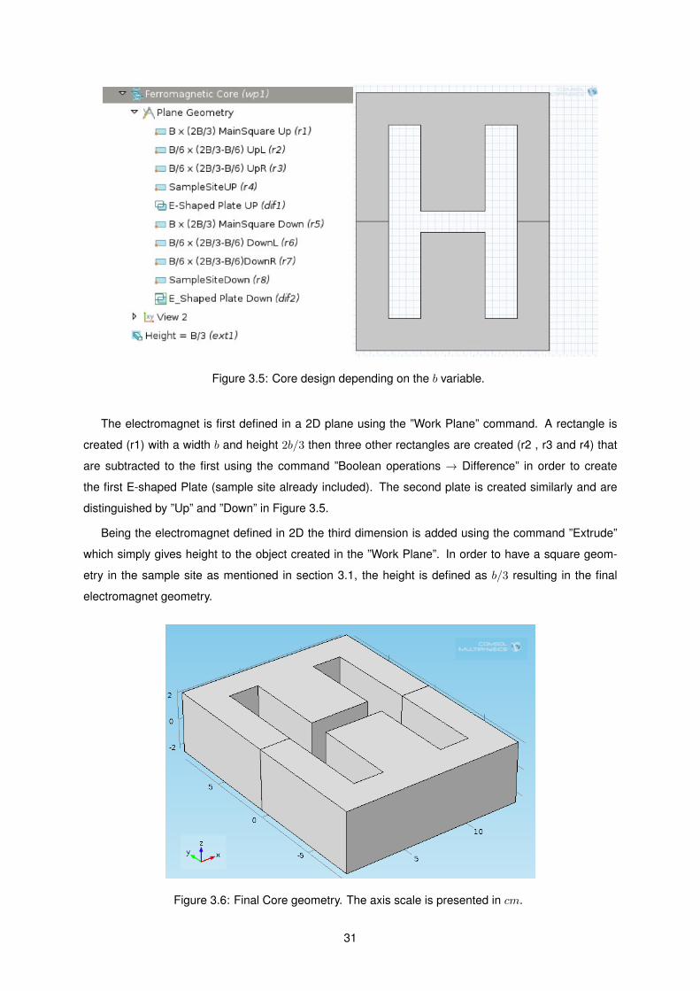
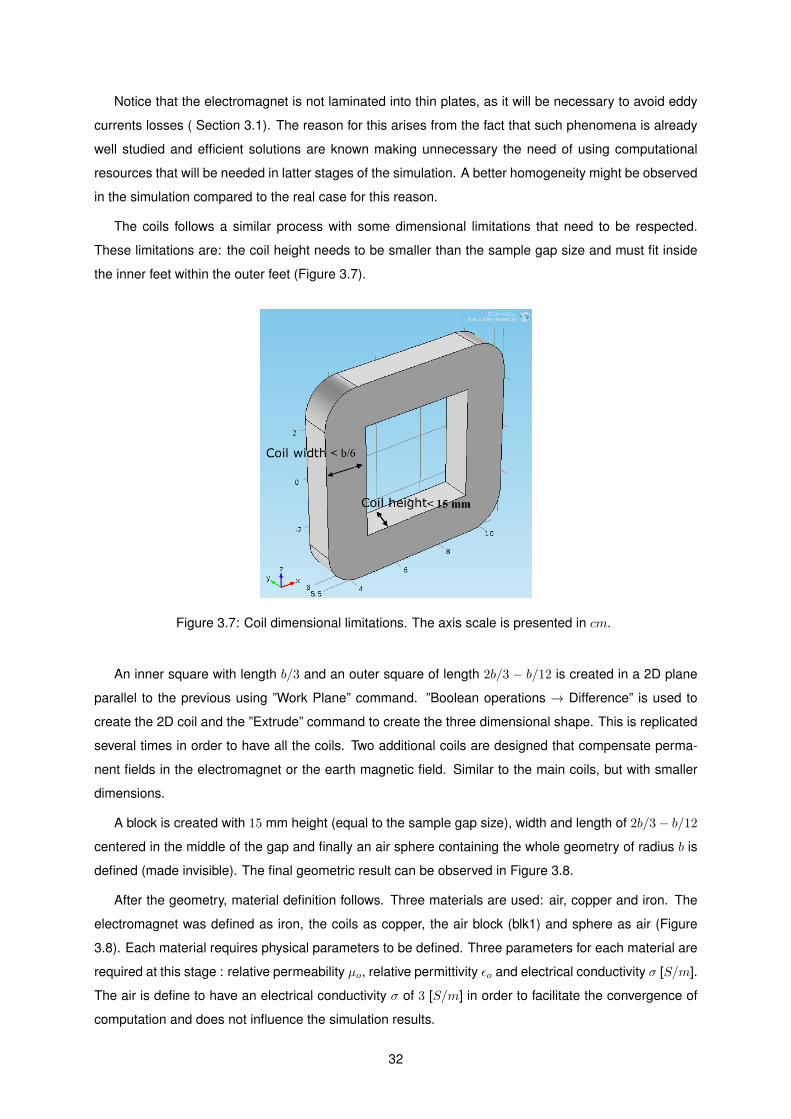
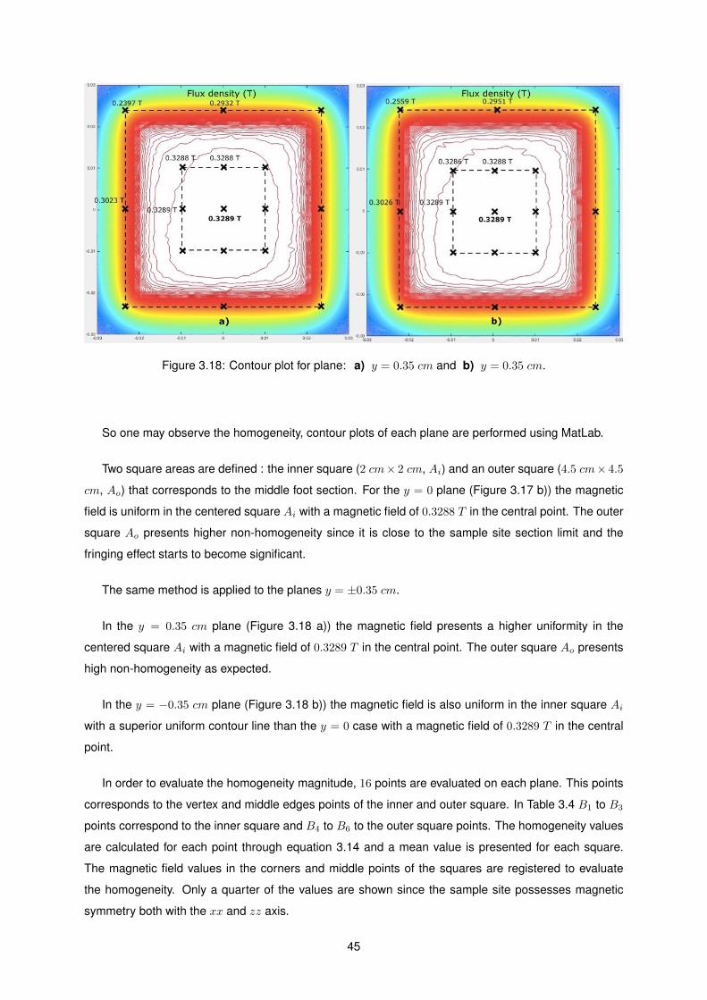
Table 3.4: Field homogeneity analysis of the y0 = 0 / y1 = 0.35 / y2 = −0.35 cm planes in the inner andouter square vertex and middle edges points. Such numerical precision in the homogeneity percentageis required otherwise it would seen a perfectly uniform surface in the inner square, which does notcorresponds to the truth.

It is concluded that in the inner square (2 cm × 2 cm) exists high homogeneity in which each layer

(y = 0, y = 0.35 cm, y = −0.35 cm) the magnetic field magnitude is By=0 = 0.3288 T , By=0.35 = 0.3289 T

By=−0.35 = 0.3289 T without existing any visible contour line in the interior. A difference in the magnetic

field between the outer planes and the middle plane is observed (±0.0001 T ). In the outer square the

same can not be observed and it becomes undesirable to analyse the sample outside the inner square.

The mean values of the homogeneity are compiled next to the previous built equipment [1] in Table

3.5. The homogeneity is proven to be acceptable with similar homogeneity results for the inner square .

Plane y coordinate Case under study ’FFC 3’

0 cm 0.22% 0.20%

Table 3.5: Homogeneity values compilation along the ’FFC 3’ results [1]. The homogeneity correspondsto the Ai square. The inner square has the same dimensions as ’FFC3’ but the outer square correspondsto the area of 6× 6 cm and cannot be compared. These is the only comparable result.

46

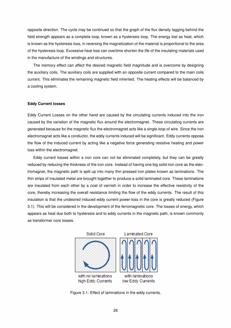
3.2.4 Fringing Effect

As mentioned before, the magnetic flux alternates between iron and air. This leads to a frigging effect

which is observed in the simulation, Figure 3.14. The magnetic flux lines cease to be straight and parallel

leading to non-uniform field. Therefore it becomes important to take this phenomenon into account.

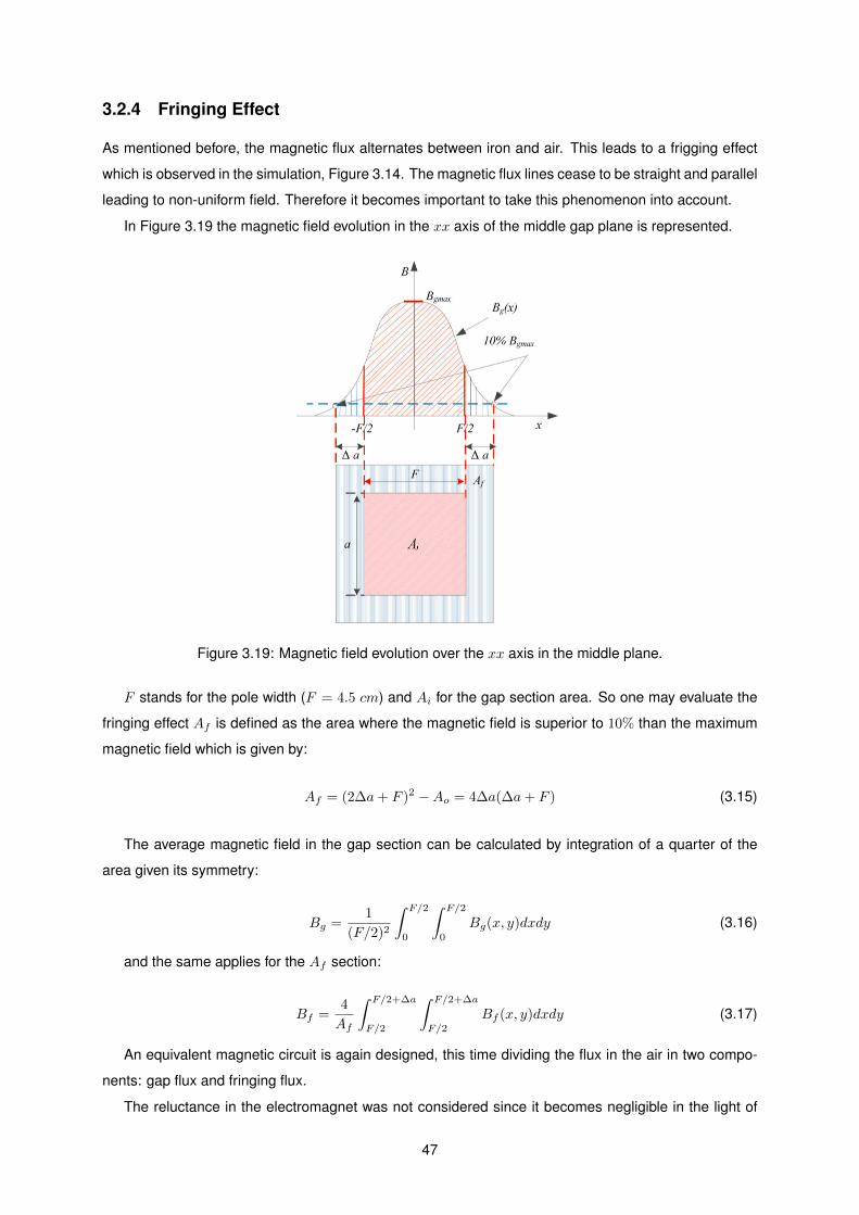
In Figure 3.19 the magnetic field evolution in the xx axis of the middle gap plane is represented.

Figure 3.19: Magnetic field evolution over the xx axis in the middle plane.

F stands for the pole width (F = 4.5 cm) and Ai for the gap section area. So one may evaluate the

fringing effect Af is defined as the area where the magnetic field is superior to 10% than the maximum

magnetic field which is given by:

Af = (2∆a+ F )2 −Ao = 4∆a(∆a+ F ) (3.15)

The average magnetic field in the gap section can be calculated by integration of a quarter of the

area given its symmetry:

Bg =1

(F/2)2

∫ F/2

0

∫ F/2

0

Bg(x, y)dxdy (3.16)

and the same applies for the Af section:

Bf =4

Af

∫ F/2+∆a

F/2

∫ F/2+∆a

F/2

Bf (x, y)dxdy (3.17)

An equivalent magnetic circuit is again designed, this time dividing the flux in the air in two compo-

nents: gap flux and fringing flux.

The reluctance in the electromagnet was not considered since it becomes negligible in the light of

47

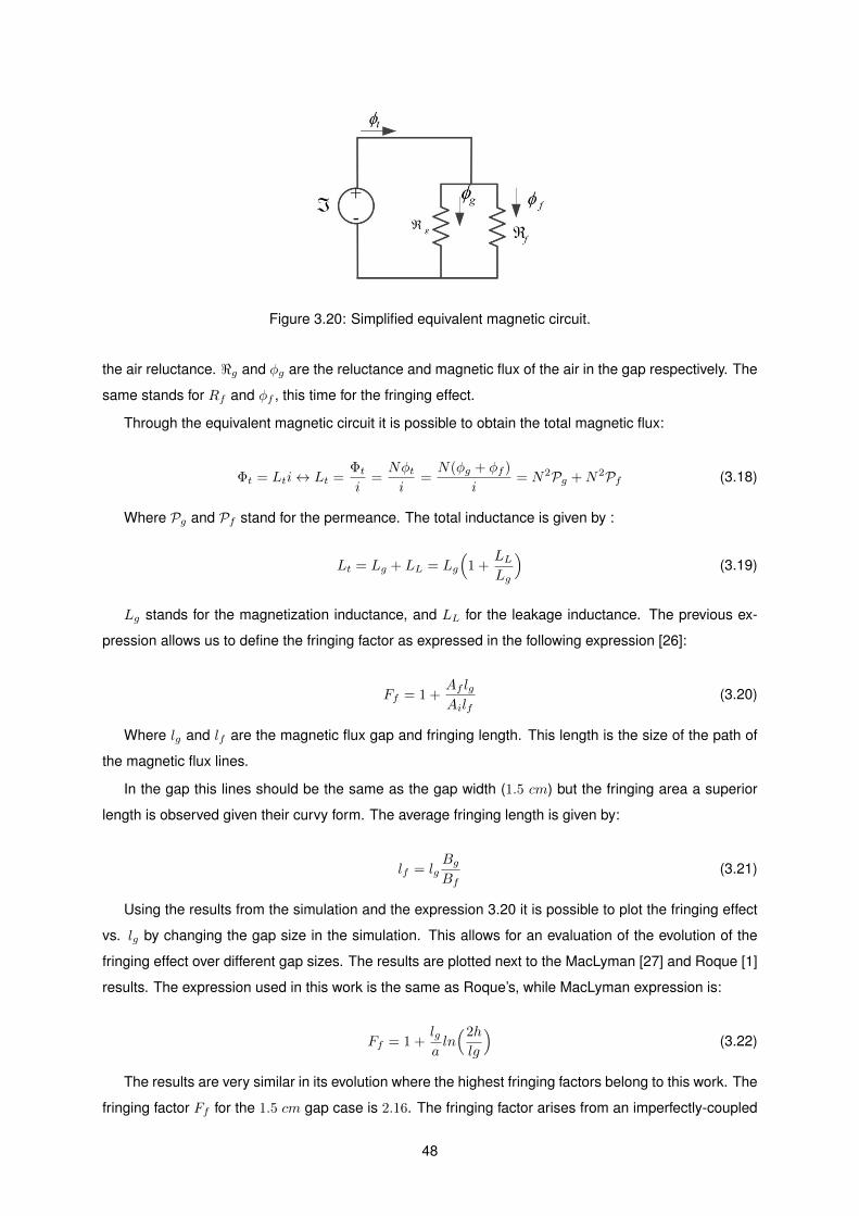
Figure 3.20: Simplified equivalent magnetic circuit.

the air reluctance. <g and φg are the reluctance and magnetic flux of the air in the gap respectively. The

same stands for Rf and φf , this time for the fringing effect.

Through the equivalent magnetic circuit it is possible to obtain the total magnetic flux:

Φt = Lti ↔ Lt =Φt

i=

Nφt

i=

N(φg + φf )

i= N2Pg +N2Pf (3.18)

Where Pg and Pf stand for the permeance. The total inductance is given by :

Lt = Lg + LL = Lg

(1 +

LL

Lg

)(3.19)

Lg stands for the magnetization inductance, and LL for the leakage inductance. The previous ex-

pression allows us to define the fringing factor as expressed in the following expression [26]:

Ff = 1 +Af lgAilf

(3.20)

Where lg and lf are the magnetic flux gap and fringing length. This length is the size of the path of

the magnetic flux lines.

In the gap this lines should be the same as the gap width (1.5 cm) but the fringing area a superior

length is observed given their curvy form. The average fringing length is given by:

lf = lgBg

Bf(3.21)

Using the results from the simulation and the expression 3.20 it is possible to plot the fringing effect

vs. lg by changing the gap size in the simulation. This allows for an evaluation of the evolution of the

fringing effect over different gap sizes. The results are plotted next to the MacLyman [27] and Roque [1]

results. The expression used in this work is the same as Roque’s, while MacLyman expression is:

Ff = 1 +lgaln(2hlg

)(3.22)

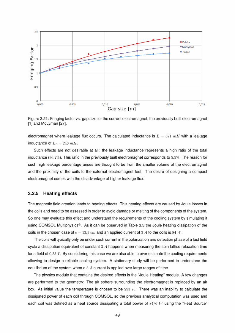
The results are very similar in its evolution where the highest fringing factors belong to this work. The

fringing factor Ff for the 1.5 cm gap case is 2.16. The fringing factor arises from an imperfectly-coupled

48

Figure 3.21: Fringing factor vs. gap size for the current electromagnet, the previously built electromagnet[1] and McLyman [27].

electromagnet where leakage flux occurs. The calculated inductance is L = 671 mH with a leakage

inductance of LL = 243 mH.

Such effects are not desirable at all: the leakage inductance represents a high ratio of the total

inductance (36.2%). This ratio in the previously built electromagnet corresponds to 5.5%. The reason for

such high leakage percentage arises are thought to be from the smaller volume of the electromagnet

and the proximity of the coils to the external electromagnet feet. The desire of designing a compact

electromagnet comes with the disadvantage of higher leakage flux.

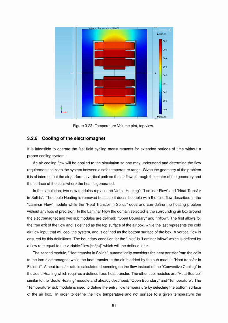
3.2.5 Heating effects

The magnetic field creation leads to heating effects. This heating effects are caused by Joule losses in

the coils and need to be assessed in order to avoid damage or melting of the components of the system.

So one may evaluate this effect and understand the requirements of the cooling system by simulating it

using COMSOL Multiphysics R©. As it can be observed in Table 3.3 the Joule heating dissipation of the

coils in the chosen case of b = 13.5 cm and an applied current of 3 A to the coils is 84 W .

The coils will typically only be under such current in the polarization and detection phase of a fast field

cycle a dissipation equivalent of constant 3 A happens when measuring the spin lattice relaxation time

for a field of 0.33 T . By considering this case we are also able to over estimate the cooling requirements

allowing to design a reliable cooling system. A stationary study will be performed to understand the

equilibrium of the system when a 3 A current is applied over large ranges of time.

The physics module that contains the desired effects is the ”Joule Heating” module. A few changes

are performed to the geometry: The air sphere surrounding the electromagnet is replaced by an air

box. As initial value the temperature is chosen to be 293 K. There was an inability to calculate the

dissipated power of each coil through COMSOL, so the previous analytical computation was used and

each coil was defined as a heat source dissipating a total power of 84/6 W using the ”Heat Source”

49

sub module. The heat is transferred to the electromagnet by thermal conduction and to the air by

convection. This is specified in the software adding the ”Heat transfer in Solids” and ”Convective Cooling”

sub modules. In the ”Heat transfer in Solids” the coils and electromagnet geometries are added and the

thermal conductivity constant is determined by the materials. For the ”Convective Cooling” the air box

surrounding the electromagnet is added and the Heat transfer coefficient is defined as h = 5 W/(m2.K)

which is the tabled value for free air convection. The last step is to define the air box boundaries at

constant 293 K using the ”Temperature” sub module by selecting the air box surfaces.

The defined problem for the Joule Heating effect can be summed up to: The electromagnet geometry

with six coils dissipate a total of 84 W surrounded by air at a temperature of 20 C. The initial tempera-

ture of the system is 20 C , the heat coefficient between the air and the geometry is 5 W/(m2.K) and

the thermal conduction between the iron and cooper is defined by the materials. Being the definition

complete, a stationary study is performed using a different mesh (uniform mesh through the whole ge-

ometry since the sample site detail is not of interest in this case). The result can be observed in Figure

3.22.

Figure 3.22: Temperature Volume plot, 3D view. The axis scale is presented in cm.

The heating effect reaches an equilibrium temperature of 302 degrees. The hottest parts correspond

to the coils and the sample site area, with lower temperatures in the borders of the electromagnet. Such

differences aren’t significant given the high conductivity of the iron. The simulation shows the expected

effects and confirm the need of a cooling system in order to avoid damages to the equipment.

50

Figure 3.23: Temperature Volume plot, top view.

3.2.6 Cooling of the electromagnet

It is infeasible to operate the fast field cycling measurements for extended periods of time without a

proper cooling system.

An air cooling flow will be applied to the simulation so one may understand and determine the flow

requirements to keep the system between a safe temperature range. Given the geometry of the problem

it is of interest that the air perform a vertical path so the air flows through the center of the geometry and

the surface of the coils where the heat is generated.

In the simulation, two new modules replace the ”Joule Heating”: ”Laminar Flow” and ”Heat Transfer

in Solids”. The Joule Heating is removed because it doesn’t couple with the fuild flow described in the

”Laminar Flow” module while the ”Heat Transfer in Solids” does and can define the heating problem

without any loss of precision. In the Laminar Flow the domain selected is the surrounding air box around

the electromagnet and two sub modules are defined: ”Open Boundary” and ”Inflow”. The first allows for

the free exit of the flow and is defined as the top surface of the air box, while the last represents the cold

air flow input that will cool the system, and is defined as the bottom surface of the box. A vertical flow is

ensured by this definitions. The boundary condition for the ”Inlet” is ”Laminar inflow” which is defined by

a flow rate equal to the variable ”flow [m3/s]” which will the defined later.

The second module, ”Heat transfer in Solids”, automatically considers the heat transfer from the coils

to the iron electromagnet while the heat transfer to the air is added by the sub module ”Heat transfer in

Fluids 1”. A heat transfer rate is calculated depending on the flow instead of the ”Convective Cooling” in

the Joule Heating which requires a defined fixed heat transfer. The other sub modules are ”Heat Source”

similar to the ”Joule Heating” module and already described, ”Open Boundary” and ”Temperature”. The

”Temperature” sub module is used to define the entry flow temperature by selecting the bottom surface

of the air box. In order to define the flow temperature and not surface to a given temperature the

51

”Discontinuous Galerkin constrains” is selected by activating the ”Advanced Physics Option”. This can

be seen in Figure 3.24 as well as the initial values definition. Both pressure and initial velocity are set at

a low value different than 0 in order to facilitate convergence, initial temperature is set as usual at 20 C.

Figure 3.24: Modules and sub modules used and defined initial values.

The last and important consideration is the ”Mesh”. Given the air flow and the sharp edges of the

geometry high gradients in velocity fields, and pressure are expected. This leads to non-convergence of

the COMSOL solvers. In order to prevent this the ”Boundary layer” option is used. This creates a thin

layer between the air domains and the solid material domains which allow for smoother transitions in the

gradients benefiting the convergence and not affecting the results. For the given case a mesh of 83767

elements is created. This defines the physics of the cooling problem, but a few observations should be

noted:

• It is desirable that the flow performs a vertical path, but this does not mean the flow begins it path

vertically. It is possible that an horizontal inlet flow is used, and the flow is forced to perform a

vertical path. Since the cooling system isn’t yet defined, an approximation is required for the air

path. A total vertical path is suitable given that the air will indeed flow through the inner geometry.

• In the real problem the flow will not assume a laminar flow, but a quite turbulent one given the

geometry and the changes the orientation of the flow. Turbulent flow is extremely expensive in

terms of computational power, and wouldn’t be feasible to simulate given the available computing

power of the machine where COMSOL Multiphysics R© is used, hence an alternative was required.

Laminar flow provides heat transfer only through conduction because in laminar flow the air is

flowing in sheets with little mixing between them. The layer of air that touches the geometry is

heated. That layer also does not mix with the other layers of air above it. The heat can only be

transferred from one layer to the next by contact (conduction). The turbulent flow has no sheets.

This means that more fresh cold gas will contact the surface resulting in a faster heat transfer

52

rate due to a larger average temperature difference between the geometry and air. Given this the

laminar flow consideration leads to an over estimative of the required flow, which is desirable in

order to allow for several hours of NMR measurements.

• The ”Inlet” and ”open boundary” are an exaggeration in terms of the available area since a compact

equipment is desired - most likely the flow will both enter and exit by considerable smaller areas.

The exaggeration of the inlet area is not a considerable effect since the majority of the air is forced

through the middle of the geometry and the smaller the inlet area the more turbulent will be the

flow, leading to improved heat transfer to the air. Finally, the exaggeration in the outlet area isn’t

considered significant since the flow has already gone through electromagnet and performed its

cooling effect.

In order to evaluate the air flow cooling effect different flow rates are computed. COMSOL allows for

parametric swept of variables and the considered values of the flow rate are : 57.6 ; 80 ; 92 ; 108 ; 158

and 170 m3/h. This was obtained after research and evaluation of different available fans in the market

that could be implemented in this case.

The defined problem for the cooling effect can be summed up to: The electromagnet geometry with

six coupled coils , each dissipating a total of 14 W at an initial temperature of 20 C. An air laminar

flow is immediately forced through the bottom of the electromagnet (in an area slightly bigger than the

electromagnet’s plane area) and leaves through the top (equal area of the inlet) cooling the geometry.

The inlet forces air at 20 C and has a defined flow rate (m3/s).

The results of the computation are 3D plots of three physical quantities: pressure, temperature and

air flow velocity. The direction of the flow can be evaluated by the velocity plots.

Figure 3.25: ”Arrow Volume” plot and two ”Slice” plots.The axis scale is presented in m.

The black arrows represent the air path, which flows from bottom to top through the geometry (Figure

3.25). The ”Slice” plots show a high velocity in the middle of the geometry (sample site). In the lateral

53

view of a single centered ”Slice” plot allows better observation of the flow velocity (Figure 3.26). The

flow assumes the highest velocity in the exit at the center and limits of the geometry. The cooling effects

occurs mainly in the bottom surface of the coils and lateral surfaces of the outer coils since higher

velocity implies enhanced heat transfer. Very low cooling occurs in the inner surfaces of the coils. An

increase in distance separating the coils would favor the air cooling.

Figure 3.26: Geometry centered ”Slice” plot, side view.

The temperature data proves that an effective cooling occurs with the air flow method. For a flow rate

of 0.03 m3/s the maximum temperature in the equilibrium corresponds to 46 C and a minimum of 32 C in the electromagnet.

Figure 3.27: Temperature ”Surface” plot. The axis scale is presented in m.

54

The highest temperature occurs in the middle of the electromagnet where the coils are placed. A

relative colder area is observed in the outer edges without being a significant gradient, proving the

high thermal conductivity of the electromagnet. This definitely is an important cooling factor since it

spreads out the heat increasing the total transferred energy to the air by increasing the contact area

where a temperature gradient exists between electromagnet - air. Such temperatures are acceptable in

the perspective that no damage is inflicted to the system when such flow rate is applied for a constant

current of 3 A. The temperature plot for a 0.03 m3/s inlet flow rate can be seen in Figure 3.27. The

bottom view of the same plot shows that this side benefits of lower temperature. This is explained by the

fact that is the surface that first interacts with the air where it is at its coldest.

Figure 3.28: Temperature ”Surface” plot, bottom view. The axis scale is presented in m.

Other flow rates were also computed where the same conclusions are observed but with different

equilibrium temperatures. The equilibrium temperatures for different flow rates are compiled in Table

3.6.

Flow m3/s Flow m3/h Max. T.(degC) Min. T. (degC)0.016 57.6 64.2 49.90.022 80 53.4 39.40.026 92 49.3 35.60.030 108 45.9 32.40.044 158 38.9 26.60.047 170 37.9 25.9

Table 3.6: Maximum (Max. T.) and minimum (Min. T.) equilibrium temperature in the electromagnet fora given flow rate.

The last set of plots correspond to the Pressure. Although this is not a crucial parameter to consider

since all the system will be constituted of solid materials that are not significantly affected by pressure

gradients it can be seen as a verification step of the correct definition of the problem. On one hand a

55

higher pressure is expected in the bottom where lower velocities occurs on the other hand lower pressure

for the top where the air assumes its higher velocity. This is confirmed by the ”Contour line” plot of Figure

(3.29).

Figure 3.29: Pressure ”Contour line” plot, side view.

This finishes the simulation phase and the development phase follows.

56

Chapter 4

Experimental Results , Assembly &

Coupled systems

In Chapter 3 the simulation of different parameters for the electromagnet were performed while evaluat-

ing the magnetic field in the sample site. This led to the decision of the most suitable parameters to be

used for the electromagnet having in mind the envisaged goal for the future spectrometer. The desired

electromagnet has a b = 13.5 cm, six coils that operate at a maximum current of 3 A, 218 turns in each

coil using a copper wire of 0.9 mm diameter.

According to COMSOL Multiphysics R© the electromagnet parameters allow the creation of a maximum

magnetic field of 0.329 T , also confirmed by the equivalent magnetic circuit and according to analytical

calculations the coils have a total ohmic resistance of 9.3 Ω and maximum joule losses of 84 W for a

current of 3 A. Field homogeneity was also evaluated as well as evaluation of the heating effect of the

dissipated heat on the electromagnet, with and without forced air flow. In this chapter it is intended to

experimentally evaluate this physical quantities provided by the simulation and analytical calculations.

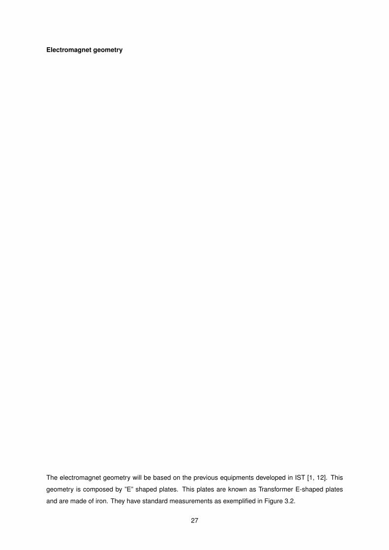
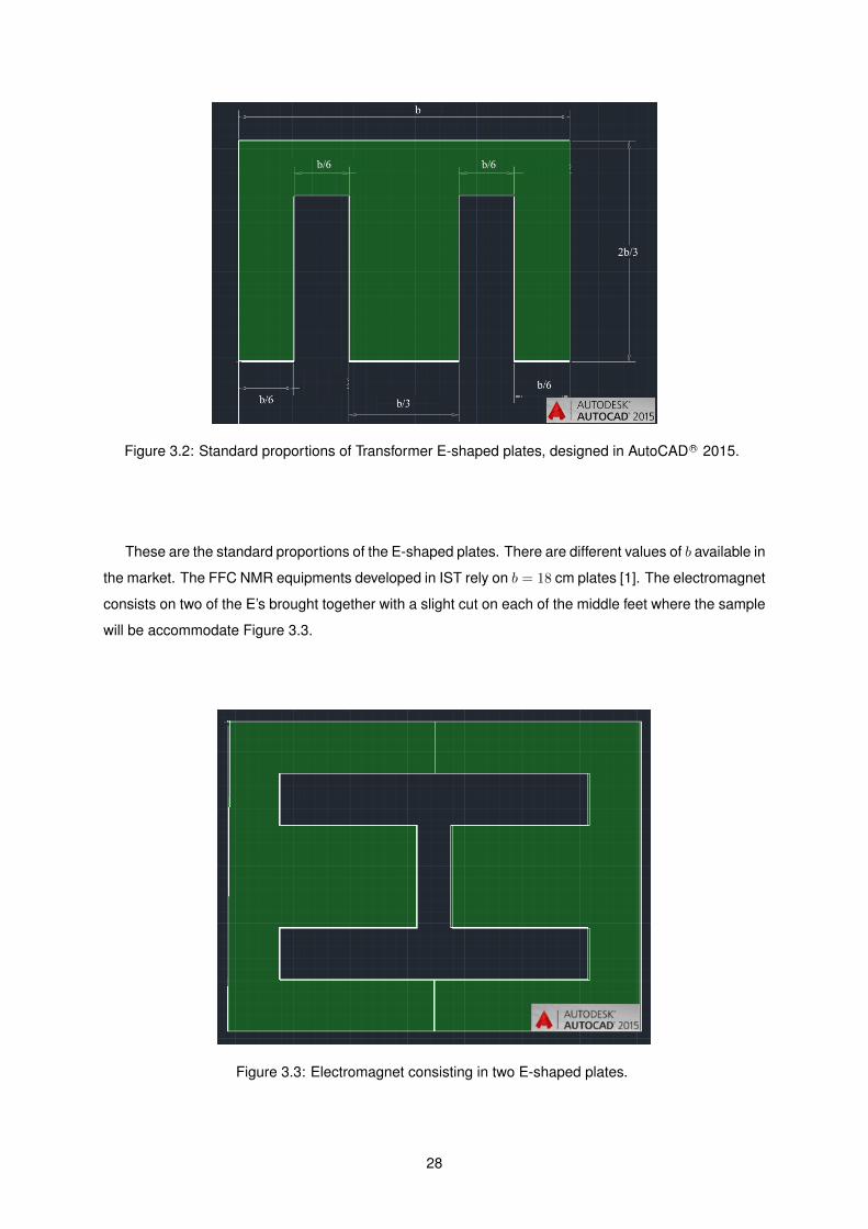
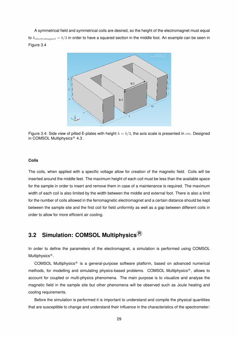
4.1 Electromagnet

The desired parameters of the electromagnet were designed and compiled. The electromagnet was

built by outsourcing all the parts: from the electromagnet to the coils, and rectification of the sample

site section. Two additional coils were added to serve the purpose of auxiliary coils, which compensate

permanent magnetizations of the electromagnet and the earth magnetic field. This coils are composed

of 430 turns each with a copper wire of 0.25mm diameter. The built electromagnet can be seen in Figure

4.1.

57

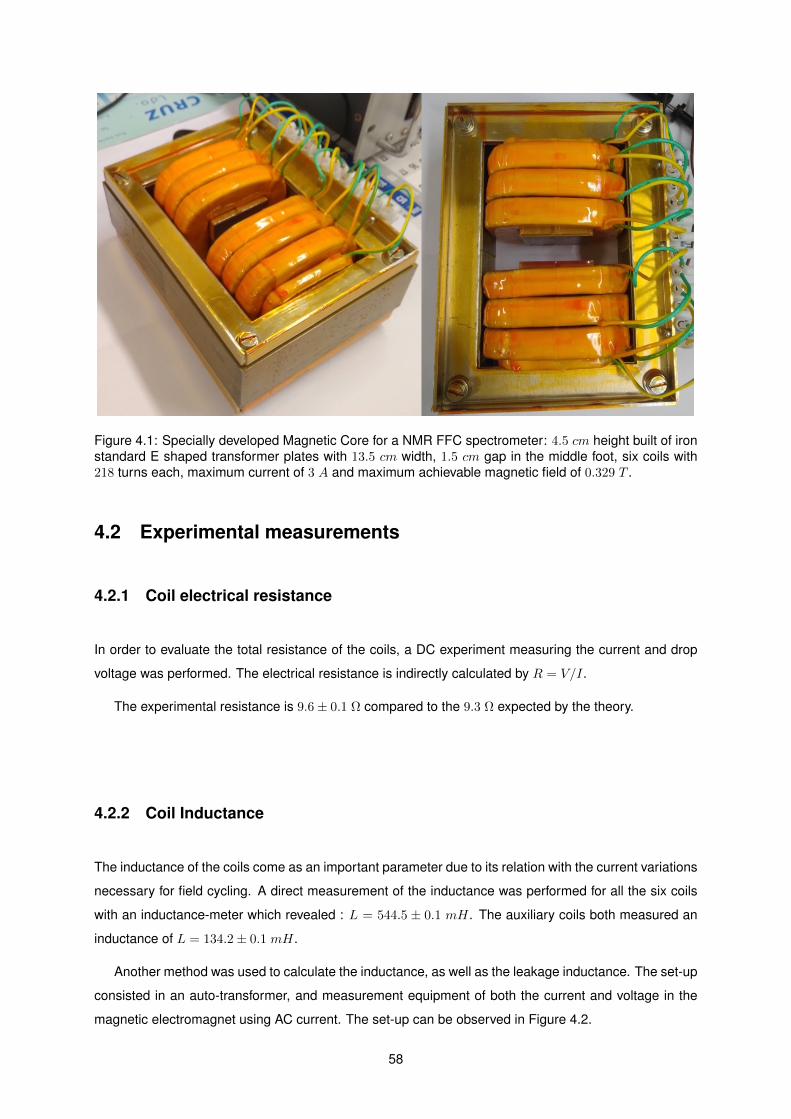
Figure 4.1: Specially developed Magnetic Core for a NMR FFC spectrometer: 4.5 cm height built of ironstandard E shaped transformer plates with 13.5 cm width, 1.5 cm gap in the middle foot, six coils with218 turns each, maximum current of 3 A and maximum achievable magnetic field of 0.329 T .

4.2 Experimental measurements

4.2.1 Coil electrical resistance

In order to evaluate the total resistance of the coils, a DC experiment measuring the current and drop

voltage was performed. The electrical resistance is indirectly calculated by R = V/I.

The experimental resistance is 9.6± 0.1 Ω compared to the 9.3 Ω expected by the theory.

4.2.2 Coil Inductance

The inductance of the coils come as an important parameter due to its relation with the current variations

necessary for field cycling. A direct measurement of the inductance was performed for all the six coils

with an inductance-meter which revealed : L = 544.5 ± 0.1 mH. The auxiliary coils both measured an

inductance of L = 134.2± 0.1 mH.

Another method was used to calculate the inductance, as well as the leakage inductance. The set-up

consisted in an auto-transformer, and measurement equipment of both the current and voltage in the

magnetic electromagnet using AC current. The set-up can be observed in Figure 4.2.

58

Figure 4.2: Experimental set-up in order to evaluate the magnetic field vs. position in the sample middleplane.

Two combination of coils were used: all six coils connected as usually (additive mode) and in another

case half the coils fed by an opposite current in order to neutralize the field created by the other half

(subtractive mode). Measuring both current and voltage , the impedance, Z can be calculated and by

knowing the resistance, the inductance L. In the subtractive mode the calculated L corresponds to the

leakage inductance LL.

I (A) V (V ) Z (Ω) L (mH)0.2 41.8 209.0 664.90.4 83.7 209.3 665.70.6 123.3 205.5 653.70.8 164.5 205.6 654.11.0 204.6 204.6 650.1

Mean value : 657.7 mH

Table 4.1: Impedance results from the additive mode.

I (A) V (V ) Z (Ω) Lleakage (mH) (L× 100)/LL%0.2 15.2 76.0 239.9 36.090.4 29.1 72.8 229.5 34.480.6 43.0 71.7 226.1 34.580.8 57.2 71.5 225.5 34.471.0 71.6 71.6 225.8 34.70

Mean Values: 229.4 mH 34.9

Table 4.2: Leakage impedance results from the subtractive mode.

Using the AC current method an inductance of L = 657.7 ± 0.1 mH was obtained, and a leakage

inductance of LL = 229.4 mH which corresponds to 34.7% of the total inductance. This confirms the

predictions of the simulation about the leakage flux. Leakage flux, as mentioned before is thought to

arise from two factors: small electromagnet volume and proximity of the coils to the external feet. This

proximity might prevent the lines to close properly and a higher distance would therefore reduce the

fringing effect and leakage ratio. The first hypothesis is confirmed by the previously built electromagnet

59

[1] given the lower fringing ratio (1.62 against the 2.16 of the current work) and leakage ratio (5.5% against

36.2% in the simulations) for a similar distance between feet (3 cm against the 2.25 of the current work)

and a bigger magnetic electromagnet (standard plates measurement of 18 cm against 13.5 cm of the

current work).

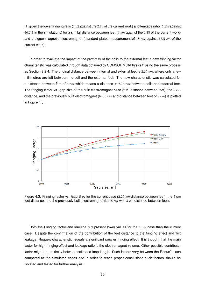
In order to evaluate the impact of the proximity of the coils to the external feet a new fringing factor

characteristic was calculated through data obtained by COMSOL MultiPhysics R© using the same process

as Section 3.2.4. The original distance between internal and external feet is 2.25 cm, where only a few

millimetres are left between the coil and the external feet. The new characteristic was calculated for

a distance between feet of 5 cm which means a distance > 2.75 cm between coils and external feet.

The fringing factor vs. gap size of the built electromagnet case (2.25 distance between feet), the 5 cm

distance, and the previously built electromagnet (b=18 cm and distance between feet of 3 cm) is plotted

in Figure 4.3.

Figure 4.3: Fringing factor vs. Gap Size for the current case (2.25 cm distance between feet), the 5 cmfeet distance, and the previously built electromagnet (b=18 cm with 3 cm distance between feet).

Both the Fringing factor and leakage flux present lower values for the 5 cm case than the current

case. Despite the confirmation of the contribution of the feet distance to the fringing effect and flux

leakage, Roque’s characteristic reveals a significant smaller fringing effect. It is thought that the main

factor for high fringing effect and leakage ratio is the electromagnet volume. Other possible contributor

factor might be proximity between coils and loop length. Such factors vary between the Roque’s case

compared to the simulated cases and in order to reach proper conclusions such factors should be

isolated and tested for further analysis.

60

4.2.3 Magnetic field magnitude measurement

The magnetic field magnitude over multiple planes vs. position was obtained through the simulation

and evaluated. An experimental evaluation of the same kind is performed. The experimental set-up

consisted in the magnetic electromagnet fed by a power supply, where both a ammeter and a voltmeter

were embedded in the circuit in order to have a thoroughly evaluation of this physical quantities. A Hall

Sensor (Model: GM-5180) was attached to a XY Table which controlled its position along the desired

area.

Figure 4.4: Experimental set-up in order to evaluate the magnetic field vs. position in the sample middleplane.

Figure 4.5: X Y table detail.

61

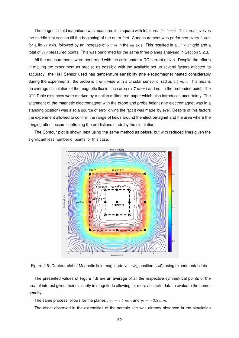
The magnetic field magnitude was measured in a square with total area 9×9 cm2. This area involves

the middle foot section till the beginning of the outer feet. A measurement was performed every 5 mm

for a fix xx axis, followed by an increase of 5 mm in the yy axis. This resulted in a 17 × 17 grid and a

total of 289 measured points. This was performed for the same three planes analysed in Section 3.2.3.

All the measurements were performed with the coils under a DC current of 3 A. Despite the efforts

in making the experiment as precise as possible with the available set-up several factors affected its

accuracy: the Hall Sensor used has temperature sensibility (the electromagnet heated considerably

during the experiment) , the probe is 4 mm wide with a circular sensor of radius 1.5 mm. This means

an average calculation of the magnetic flux in such area (≈ 7 mm2) and not in the pretended point. The

XY Table distances were marked by a nail in millimetred paper which also introduces uncertainty. The

alignment of the magnetic electromagnet with the probe and probe height (the electromagnet was in a

standing position) was also a source of error giving the fact it was made ’by eye’. Despite of this factors

the experiment allowed to confirm the range of fields around the electromagnet and the area where the

fringing effect occurs confirming the predictions made by the simulation.

The Contour plot is shown next using the same method as before, but with reduced lines given the

significant less number of points for this case.

Figure 4.6: Contour plot of Magnetic field magnitude vs. x&y position (z=0) using experimental data.

The presented values of Figure 4.6 are an average of all the respective symmetrical points of the

area of interest given their similarity in magnitude allowing for more accurate data to evaluate the homo-

geneity.

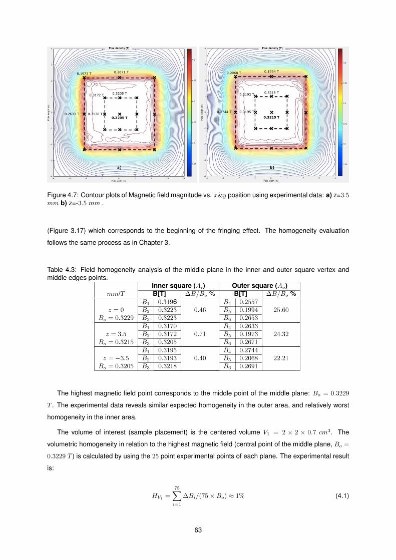
The same process follows for the planes : y1 = 3.5 mm and y2 = −3.5 mm.

The effect observed in the extremities of the sample site was already observed in the simulation

62

Figure 4.7: Contour plots of Magnetic field magnitude vs. x&y position using experimental data: a) z=3.5mm b) z=-3.5 mm .

(Figure 3.17) which corresponds to the beginning of the fringing effect. The homogeneity evaluation

follows the same process as in Chapter 3.

Table 4.3: Field homogeneity analysis of the middle plane in the inner and outer square vertex andmiddle edges points.

Inner square (Ai) Outer square (Ao)mm/T B[T] ∆B/Bo % B[T] ∆B/Bo %

B1 0.3196 B4 0.2557z = 0 B2 0.3223 0.46 B5 0.1994 25.60

Bo = 0.3229 B3 0.3223 B6 0.2653B1 0.3170 B4 0.2633

z = 3.5 B2 0.3172 0.71 B5 0.1973 24.32Bo = 0.3215 B3 0.3205 B6 0.2671

B1 0.3195 B4 0.2744z = −3.5 B2 0.3193 0.40 B5 0.2068 22.21

Bo = 0.3205 B3 0.3218 B6 0.2691

The highest magnetic field point corresponds to the middle point of the middle plane: Bo = 0.3229

T . The experimental data reveals similar expected homogeneity in the outer area, and relatively worst

homogeneity in the inner area.

The volume of interest (sample placement) is the centered volume V1 = 2 × 2 × 0.7 cm3. The

volumetric homogeneity in relation to the highest magnetic field (central point of the middle plane, Bo =

0.3229 T ) is calculated by using the 25 point experimental points of each plane. The experimental result

is:

HV1 =

75∑i=1

∆Bi/(75×Bo) ≈ 1% (4.1)

63

4.3 Coupled systems, assembly and casing

The electromagnet will operate inside a casing along with the remaining support systems which are:

Sample Heating; Cooling; RF coil.

The electromagnet was not fully built during the length of this work. Despite of this fact the projection

of missing parts was performed as far as the time allowed. For the rest of this Chapter, gathered

information, projections and considerations for the rest of the spectrometer are described.

4.3.1 Sample heating

The spectrometer must be able to heat the test samples to temperatures up to 150 C. This is achieved

by heated air and such system must be designed in order not to heat the electromagnet or other spec-

trometer components.

The components that constitute the heating system are: Input valve, air heater, a specially designed

component, glass structure, connection tubes and a thermocouple. The input valve function is to receive

air at room temperature from an outer independent system and guide it to the air heater, and is yet to

be defined. The air is heated by the use of a resistance in a tube. The acquired model is: Marathon-IN

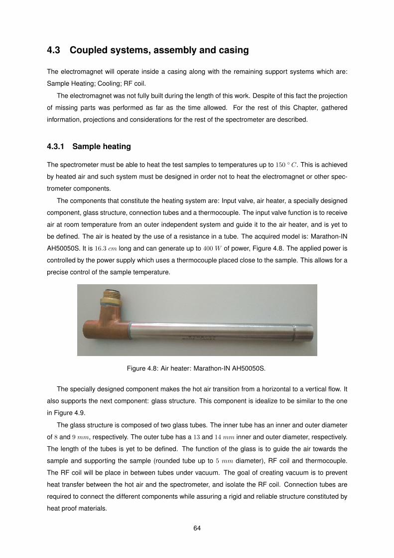
AH50050S. It is 16.3 cm long and can generate up to 400 W of power, Figure 4.8. The applied power is

controlled by the power supply which uses a thermocouple placed close to the sample. This allows for a

precise control of the sample temperature.

Figure 4.8: Air heater: Marathon-IN AH50050S.

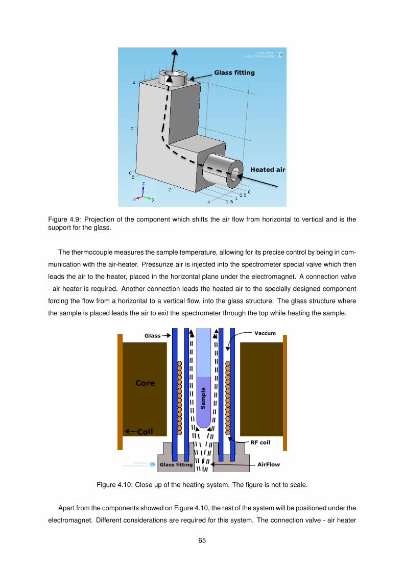
The specially designed component makes the hot air transition from a horizontal to a vertical flow. It

also supports the next component: glass structure. This component is idealize to be similar to the one

in Figure 4.9.

The glass structure is composed of two glass tubes. The inner tube has an inner and outer diameter

of 8 and 9 mm, respectively. The outer tube has a 13 and 14 mm inner and outer diameter, respectively.

The length of the tubes is yet to be defined. The function of the glass is to guide the air towards the

sample and supporting the sample (rounded tube up to 5 mm diameter), RF coil and thermocouple.

The RF coil will be place in between tubes under vacuum. The goal of creating vacuum is to prevent

heat transfer between the hot air and the spectrometer, and isolate the RF coil. Connection tubes are

required to connect the different components while assuring a rigid and reliable structure constituted by

heat proof materials.

64

Figure 4.9: Projection of the component which shifts the air flow from horizontal to vertical and is thesupport for the glass.

The thermocouple measures the sample temperature, allowing for its precise control by being in com-

munication with the air-heater. Pressurize air is injected into the spectrometer special valve which then

leads the air to the heater, placed in the horizontal plane under the electromagnet. A connection valve

- air heater is required. Another connection leads the heated air to the specially designed component

forcing the flow from a horizontal to a vertical flow, into the glass structure. The glass structure where

the sample is placed leads the air to exit the spectrometer through the top while heating the sample.

Figure 4.10: Close up of the heating system. The figure is not to scale.

Apart from the components showed on Figure 4.10, the rest of the system will be positioned under the

electromagnet. Different considerations are required for this system. The connection valve - air heater

65

is to be made by a flexible tube of any material as long as the connection is reliable and well coupled

in both ends but the connection between the end of the air-heater to a component yet to be designed

leads air at high temperature and an according material must be used. This component is required to

have a rigid structure able to provide a steady support of the glass, to handle high temperatures and

to be fixed on the basis of the spectrometer. Positioning of the sample and RF coil must be within the

volume centered in the electromagnet gap of dimensions: 2 × 2 × 0.7 cm3 where the magnetic field

presents its higher homogeneity. This is achieved by centering the glass structure according to Figure

4.11 (electromagnet top view) and making sure the middle of the RF coil is positioned in the center of

the gap in the vertical plane.

Figure 4.11: Top view of the electromagnet and heating system. Centered positioning of the glassstructure.

4.3.2 Radio Frequency Coil

The Radio frequency coil allows for magnetization shifts and signal acquisition. The Radio frequency

circuit is constituted by a coil and a capacitor which can both apply a RF pulse and receive NMR signals.

For the correct acquisition of NMR results, both the LC circuit , applied signal to the RF coil and sample’s1H Larmor frequency need to be in resonance.

Despite the electromagnet is designed to reach a maximum magnetic field of ≈ 0.33 T the current

power supply is designed according to the previous versions of the FFC equipments. The Radio Fre-

quency control system of the power supply is matched to the previous maximum magnetic field and

Larmor frequency: 0.21 T and 8.862 MHz. This means that given the available power supply the elec-

tromagnet is required to operate at a maximum field of 0.21 T and the RF generator matched to a

resonance frequency of 8.862 MHz.

The RF coil should be small enough to fit the electromagnet gap but big enough to allow for sample

insertion. The coil is placed around the inner edge of the outer glass tube. It is intended to use a 0.4

66

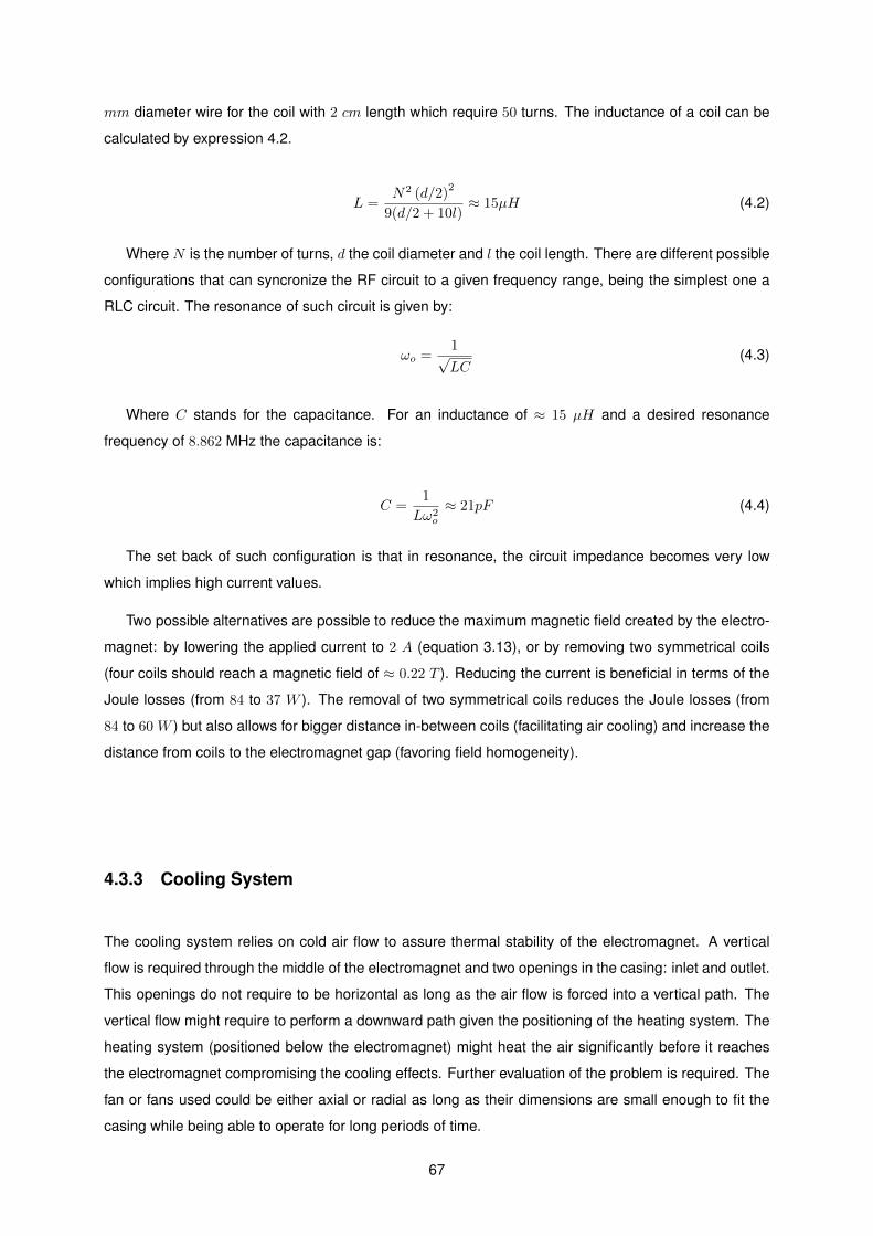
mm diameter wire for the coil with 2 cm length which require 50 turns. The inductance of a coil can be

calculated by expression 4.2.

L =N2 (d/2)

2

9(d/2 + 10l)≈ 15µH (4.2)

Where N is the number of turns, d the coil diameter and l the coil length. There are different possible

configurations that can syncronize the RF circuit to a given frequency range, being the simplest one a

RLC circuit. The resonance of such circuit is given by:

ωo =1√LC

(4.3)

Where C stands for the capacitance. For an inductance of ≈ 15 µH and a desired resonance

frequency of 8.862 MHz the capacitance is:

C =1

Lω2o

≈ 21pF (4.4)

The set back of such configuration is that in resonance, the circuit impedance becomes very low

which implies high current values.

Two possible alternatives are possible to reduce the maximum magnetic field created by the electro-

magnet: by lowering the applied current to 2 A (equation 3.13), or by removing two symmetrical coils

(four coils should reach a magnetic field of ≈ 0.22 T ). Reducing the current is beneficial in terms of the

Joule losses (from 84 to 37 W ). The removal of two symmetrical coils reduces the Joule losses (from

84 to 60 W ) but also allows for bigger distance in-between coils (facilitating air cooling) and increase the

distance from coils to the electromagnet gap (favoring field homogeneity).

4.3.3 Cooling System

The cooling system relies on cold air flow to assure thermal stability of the electromagnet. A vertical

flow is required through the middle of the electromagnet and two openings in the casing: inlet and outlet.

This openings do not require to be horizontal as long as the air flow is forced into a vertical path. The

vertical flow might require to perform a downward path given the positioning of the heating system. The

heating system (positioned below the electromagnet) might heat the air significantly before it reaches

the electromagnet compromising the cooling effects. Further evaluation of the problem is required. The

fan or fans used could be either axial or radial as long as their dimensions are small enough to fit the

casing while being able to operate for long periods of time.

67

4.3.4 Assembly

The electromagnet and coupled systems are intended to be assembled separately from the power sup-

ply. Currently the hypothesis of using a rectangular case of similar horizontal area as the electromagnet,

but with additional height is under evaluation. The electromagnet is projected to be in the middle height

of the case where the cooling system is placed above the electromagnet and the heating system and

remaining systems under the electromagnet.

Openings in the case are required for air inlet and outlet. The inlet has the possibility to be in the

top surface of the case or in upper lateral sides. For the outlet, openings in the bottom lateral sides

are feasible as long as connecting wires aren’t in contact with the existing hot air. The horizontal area

must be enough to correctly accommodate the heating system or extra space is necessary. An extra

opening is necessary for sample insertion. The height of the case depends on the occupied volume by

the heating system and cooling system. This relative positioning allows for the air to flow through the

electromagnet, cooling it and the air heater ensuring thermal stability of all the components.

The power supply and pressurized air connections are to be made in the back of the spectrometer

and accommodated in the bottom of the spectrometer.

68

Chapter 5

Conclusions

The smallest FFC NMR electromagnet up to date was achieved, with high homogeneity in the sample

site and is designed to operate within the magnetic field range of 0 and 0.33 T . As a starting point the

three-dimensional numerical simulation was performed using COMSOL Multiphysics R© which allowed

to evaluate the magnetic field distribution in the sample site as well as thermal effects and air cooling

requirements. The simulation allowed to analyse different configurations leading to a reduced volume

electromagnet with dimensions being : 13.5× 18× 4.5 cm3.

Given the geometry configuration of the electromagnet fringing effects are observed. The fringing ef-

fect arises from the transitions iron-air, and different factors influence the magnitude of this phenomenon.

Through the simulation it was possible to sweep the gap size between 0 to 2 cm for different distances

between inner and outer feet allowing to observe the fringing effect evolution. The fringing effect reduces

field uniformity and homogeneity which comes as harmful for FFC NMR measurements. Despite of the

fringing effect high homogeneity is observed in the inner area of the sample site, evaluated both through

simulation and experimental results. No similar experimental data is known to exist for homogeneity

comparison, but comparing simulation results similar homogeneity values were obtained.

Thermal effects and cooling requirements were evaluated allowing for the design of feasible systems.

The computational simulation allowed to estimate air flow rates for safe measurements over extended

periods of time. The sample heating system was projected and some components acquired and defined.

The sample heating system design allowed for the definition of the RF circuit and specific coil and

capacitor parameters.

The improvements of the FFC magnet relatively to the previous FFC versions developed in IST are

a 60% decrease in electromagnet’s volume and weight, decrease in the applied current to the main coils

(40%) and increase in the maximum achievable magnetic field by 50%. The disadvantage of reduced

volume electromagnet (compared to the previous versions) is in the leakage flux, which is significant (≈

1/3 of the total flux).

69

The advantages of the developed FFC magnet relatively to the generality of magnets are:

• Reduced electromagnet’s volume and weight

• Low power consumption

• High homogeneity profile

• Feasible and low power cooling system

5.1 Future Work

During the length of this project different ideas came up for future work.

The first steps consists in finishing the spectrometer:

• Developing and implementation and assembly: sample heating, RF circuit, cooling system

• Auxiliary coils tuning to eliminate residual magnetic fields of the electromagnet

• Conjugation of the magnet and power supply in order to achieve fully functional FFC NMR spec-

trometer

• Perform NMR experiments using the the spectrometer

Beside the conclusion of the spectrometer there is room for improvement in other aspects. A more

detailed and precise experimental homogeneity evaluation method is desired in order for better magnetic

field mapping. A further evaluation of construction parameters such as coil positioning, E-transformer

plate dimensions, number of coils would allow a better understanding of fringing effect and leakage flux

reduction solutions. The current power supply is matched for a maximum detection frequency of 8.862

MHz where the magnet is able to reach higher values. An upgrade in its features in order to allow for the

use of magnet full capacities is desired.

70

Bibliography

[1] A. Roque. Espectrmetro de RMN de CCR com utilizao de supercondutores no magneto. PhD

thesis, Instituto Superior Tecnico, Universidade de Lisboa, 2014.

[2] C. Job, J. Zajicek, and M. F. Brown. Fast fieldcycling nuclear magnetic resonance spectrometer.

Review of Scientific Instruments, 67(6):2113–2122, 1996. doi: 10.1063/1.1147024. URL http:

//dx.doi.org/10.1063/1.1147024.

[3] M. Blanz, T. J. Rayner, and J. A. S. Smith. A fast field-cycling nmr/nqr spectrometer. Measurement

Science and Technology, 4(1):48, 1993. URL http://stacks.iop.org/0957-0233/4/i=1/a=009.

[4] K. Schweikert, R. Krieg, and F. Noack. A high-field air-cored magnet coil design for fast-

field-cycling nmr. Journal of Magnetic Resonance (1969), 78(1):77 – 96, 1988. ISSN 0022-

2364. doi: http://dx.doi.org/10.1016/0022-2364(88)90158-8. URL http://www.sciencedirect.

com/science/article/pii/0022236488901588.

[5] H. Stork, M. Ditter, H. Pler, A. Privalov, and F. Fujara. High temperature mechanical field-cycling

setup. Journal of Magnetic Resonance, 192(2):173 – 176, 2008. ISSN 1090-7807. doi: http:

//dx.doi.org/10.1016/j.jmr.2008.02.017. URL http://www.sciencedirect.com/science/article/

pii/S1090780708000621.

[6] B. Kresse, A. Privalov, and F. Fujara. Nmr field-cycling at ultralow magnetic fields. Solid State

Nuclear Magnetic Resonance, 40(4):134 – 137, 2011. ISSN 0926-2040. doi: http://dx.doi.

org/10.1016/j.ssnmr.2011.10.002. URL http://www.sciencedirect.com/science/article/pii/

S0926204011001019.

[7] A. Privalov, S. Dvinskikh, and H.-M. Vieth. Coil design for large-volume high-b1homogene-

ity for solid-state nmr applications. Journal of Magnetic Resonance, Series A, 123(2):157 –

160, 1996. ISSN 1064-1858. doi: http://dx.doi.org/10.1006/jmra.1996.0229. URL http://www.

sciencedirect.com/science/article/pii/S1064185896902296.

[8] O. Lips, A. Privalov, S. Dvinskikh, and F. Fujara. Magnet design with high b0 homogeneity for

fast-field-cycling nmr applications. Journal of Magnetic Resonance, 149(1):22 – 28, 2001. ISSN

1090-7807. doi: http://dx.doi.org/10.1006/jmre.2000.2279. URL http://www.sciencedirect.com/

science/article/pii/S1090780700922791.

71

[9] F. Noack. Nmr field-cycling spectroscopy: principles and aplications. Progress in Nuclear Mag-

netic Resonance Spectroscopy, 18(3):171 – 276, 1986. ISSN 0079-6565. doi: http://dx.doi.org/

10.1016/0079-6565(86)80004-8. URL http://www.sciencedirect.com/science/article/pii/

0079656586800048.

[10] D. M. Sousa, G. D. Marques, P. J. Sebastiao, and A. C. Ribeiro. New isolated gate bipolar transistor

two-quadrant chopper power supply for a fast field cycling nuclear magnetic resonance spectrom-

eter. Review of Scientific Instruments, 74(10):4521–4528, 2003. doi: 10.1063/1.1610785. URL

http://dx.doi.org/10.1063/1.1610785.

[11] D. Sousa, P. Fernandes, G. Marques, A. Ribeiro, and P. Sebastiao. Novel pulsed switched power

supply for a fast field cycling nmr spectrometer. Solid State Nuclear Magnetic Resonance, 25(1):

160 – 166, 2004. ISSN 0926-2040. doi: http://dx.doi.org/10.1016/j.ssnmr.2003.03.026. URL http:

//www.sciencedirect.com/science/article/pii/S0926204003001012. 31st Congress Ampere,

Magnetic Resonance and Related Phenomena.

[12] Desktop fast-field cycling nuclear magnetic resonance relaxometer. Solid State Nuclear Magnetic

Resonance, 38(1):36 – 43, 2010. ISSN 0926-2040. doi: http://dx.doi.org/10.1016/j.ssnmr.2010.07.

001. URL http://www.sciencedirect.com/science/article/pii/S0926204010000457.

[13] D. Plendl, M. Fujara, A. F. Privalov, and F. Fujara. Energy efficient iron based electronic field cycling

magnet. Journal of Magnetic Resonance, 198(2):183 – 187, 2009. ISSN 1090-7807. doi: http:

//dx.doi.org/10.1016/j.jmr.2009.02.004. URL http://www.sciencedirect.com/science/article/

pii/S1090780709000433.

[14] R. Kimmich and E. Anoardo. Field-cycling nmr relaxometry. Progress in Nuclear Mag-

netic Resonance Spectroscopy, 44(3):257 – 320, 2004. ISSN 0079-6565. doi: http://dx.doi.

org/10.1016/j.pnmrs.2004.03.002. URL http://www.sciencedirect.com/science/article/pii/

S0079656504000196.

[15] F. Fujara, D. Kruk, and A. F. Privalov. Solid state field-cycling nmr relaxometry: Instrumental im-

provements and new applications. Progress in Nuclear Magnetic Resonance Spectroscopy, 82:39

– 69, 2014. doi: http://dx.doi.org/10.1016/j.pnmrs.2014.08.002. URL http://www.sciencedirect.

com/science/article/pii/S0079656514000594.

[16] N. Jacobsen. NMR spectroscopy explained. John Wiley and Sons, 2007.

[17] F. Bloch, W. W. Hansen, and M. Packard. Nuclear induction. Phys. Rev., 69:127–127, Feb 1946.

doi: 10.1103/PhysRev.69.127. URL https://link.aps.org/doi/10.1103/PhysRev.69.127.

[18] A. Abragam. The principles of nuclear magnetism. American Journal of Physics, 29(12):860–861,

1961. doi: 10.1119/1.1937646. URL http://dx.doi.org/10.1119/1.1937646.

[19] M. I. of Technology. Nmr frequency table. Department of Chemistry, 2012.

[20] Relaxation (nmr). https://en.wikipedia.org/wiki/RelaxationNMR.

72

[21] N. Dias. Nuclear magnetic resonance study of molecular interaction of ionic liquids with aromatic

compounds. Master’s thesis, Instituto Superior Tecnico - Universidade de Lisboa, 2013.

[22] T. C. FARRAR and E. D. BECKER. Chapter 1 - basic concepts in nmr. In T. C. FARRAR and E. D.

BECKER, editors, Pulse and Fourier Transform NMR, pages 1 – 17. Academic Press, San Diego,

1971. ISBN 978-0-12-249650-9. doi: https://doi.org/10.1016/B978-0-08-091812-9.50006-5. URL

http://www.sciencedirect.com/science/article/pii/B9780080918129500065.

[23] H. Reich. Relaxation in nmr spectroscopy. U.Wisc. Chem., (605).

[24] N. Bloembergen, E. M. Purcell, and R. V. Pound. Relaxation effects in nuclear magnetic resonance

absorption. Phys. Rev., 73:679–712, Apr 1948. doi: 10.1103/PhysRev.73.679. URL https://

link.aps.org/doi/10.1103/PhysRev.73.679.

[25] Kimmich. NMR Tomography, Diffusometry, Relaxometry. John Wiley Sons, Ltd, 2007.

doi: 10.1002/9780470034590.emrhp1028. URL http://dx.doi.org/10.1002/9780470034590.

emrhp1028.

[26] Characterization of the fringing window of a magnetic core. EUROCON, 2011.

[27] M. C. W. T. Transformer and Inductor Design Handbook. Marcel Dekker, 1988.

73

74

Appendix A

Simulation Tutorial

A file containing the geometry is available. The file can be opened in every version equal or superior to

COMSOL 4.3. In order to obtain the geometry contact the supervisors of this thesis or myself via e-mail:

pedrovideira@live.com.pt.

The provided file contains a geometry specified over the variable b. Other variables are used such

as ”g” - gap size, ”aux” - height of the auxiliary coil, ”cg” - distance between coils. This can be changed

in the ”Model Builder” section , under ”Global Definitions” in ”Parameters”. All the geometry will scale

according to this parameters. After a variation of each parameter, a geometry analysis is necessary to

verify the correct positioning of the coils. In case more or less coils are desired simply duplicate the

existing ones inserting their desired position or disable them. The materials are already defined and can

be seen in ”Materials”.

I will now describe how I obtained the results presented for the previous specific case.

A.1 Magnetic Field

Open the file ”ElectromagnetGeometry.mph”

Right-Click on ”Model1” → ”Add Physics”

Select ”Magnetic Fields(mf)” , press ”Next”

Select ”Stationary Study” and press ”finish”.

The magnetic field module is added.

By right-clicking in ”Magnetic fields (mf)” add ”Multi-Turn Coil Domain”

In the ”Multi-Turn Coil Domain 1” select the desired coil and add it in the ”Domain Selection”

In ”Material Type” choose ”From Material”

In ”Coil Type” choose ”Circular”.

For the ”Multi-Turn Coil Domain” module:

The coil conductivity already uses the cooper value.

In ”Number of Turns” insert ”N ”

In the ”Coil wire cross-section area” insert ”ws”

75

In ”Coil Excitation” choose ”Current” and for the Coilcurrent insert ”Icoil”

These variables are specified in ”Parameters” with the rest of the variables.

Right Click ”Multi-Turn Coil Domain 1” and choose ”Edges” → ”Reference Edge”.

Clear the selection and select the current path by choosing the one of the outer edges. An example

can be seen in Fig. A.1.

Figure A.1: Chosen current path.

Repeat this process for each of the coils.

A.1.1 Mesh

The mesh module is usually under the physics modules, or can be added the same way as physics

modules. In the ”Mesh Settings” choose ”User-Controlled Mesh”.

Under the Mesh module choose ”Free Tetrahedral 1” and in ”Domain Selection” choose the air box

placed in the sample site. High resolution is desired in this space which implies a detailed mesh. Right-

click ”Free Tetrahedral 1” and choose ”Size”. In the ”Element Size” choose ”Custom”. In the ”Element

Size Parameters” define ”maximum element size” as ”0.003” and ”minimum element size” as ”0.0001”.

Add another ”Free Tetrahedral” by right clicking in ”Mesh” and a ”Size by right-clicking on ”Free Tetrahe-

dral”. In the ”Geometry Entity Selection” choose select all the remaining components. Choose ”Custom”

in ”Element Size” and define ”maximum element size” as ”0.02” and ”minimum element size” as ”0.005”.

In ”Study 1” under the ”Mesh” right-click and choose ”Compute”. This will produce a ”multi-slice” plot

in the ”Results”. Other plots are available but need to be added.

76

A.2 Heating Effect

Using the same method as before add the Physics Module ”Heat Transfer in Solids”.

Right-clicking ”Heat Transfer in Solids” add ”Heat Source”.

In the ”Domain Selection” add all the main coils.

In ”Heat Source” choose ”Total Power” and define the total power dissipated by the coils, in this case

84 W .

Right-clicking ”Heat Transfer in Solids” add ”Convective Cooling”.

In the ”Domain Selection” add the surface of the outer air box containing the whole geometry.

Define the ”Heat transfer coefficient” as 5 W/(m2K).

Both the ”Magnetic Field” and ”Heat Transfer in Solids” will be solved this way. For quicker com-

putation deselected ”Magnetic Field” in the ”Step 1: Stationary”. The air box in the sample site does

not require such a detailed mesh for heating effects evaluation and new values for this box ”maximum

element size” and ”minimum element size” should be selected.

Plots will be created after computation.

A.3 Cooling Effects

Using the same method as before add the Physics Module ”Laminar Flow”.

Right-clicking ”Laminar Flow” add ”Open Boundary” and ”Inlet”.

In the ”Open Boundary” choose the top surface of the surrounding air box in the ”Domain Selection”.

For the ”Inlet” choose the bottom surface of the surrounding air box in the ”Domain Selection”.

For the ”Boundary Condition” choose ”Laminar Inflow”

A new section will appear ”Laminar Inflow” choose ”Flow rate” and give it the desired value.

In the initial values define the pressure to 0.0001 and ”Velocity Field” to 0.01 in the zz component.

By right-clicking in the ”Heat Transfer in Solids” add ”Heat Transfer in Fluids” and delete the ”Convec-

tive Cooling”.

In the ”Domain Selection” add the outer air box. In the ”Velocity field” choose ”Velocity Field (spf/fp1)”.

This couples the two physical effects of this section.

Right-clicking ”Heat Transfer in Solids” add ”Open Boundary” and ”Temperature”.

In the ”Open Boundary” choose the top surface of the surrounding air box in the ”Domain Selection”.

For the ”Temperature” choose the bottom surface of the surrounding air box in the ”Domain Selec-

tion”.

Under the ”Model builder” tab choose ”Advanced Physics Options”, go back to ”Temperature”, Fig.

A.2. A new module appears ”Constrains Settings”. Choose ”Discontinuous Galerkin Constrains”. This

defines the flow temperature and not the air surface.

In the materials ”Dynamic Viscosity” parameter of iron and copper need to be defined, enter ”0”.

77

Figure A.2: How to activate the ”Discontinuous Galerkin Constrains” option.

A.3.1 Mesh

Delete the mesh and create a new one. For the whole geometry define a ”User-Defined” with ”Element

Size Parameters”: ”maximum element size” as ”0.03” and ”minimum element size” as ”0.008”. Add

”Boundary layer” by right-clicking in ”Mesh”.

Some problems in the convergence of this specific problem might arise. Try a different mesh or

slightly different initial values. After a long computation period, plots will be created.

The simultaneous computation of all the phenomena was never performed given the available com-

puter.

78