Fast MCMC Algorithms on Polytopes

Raaz Dwivedi, Department of EECS

Joint work with Yuansi Chen Martin Wainwright Bin Yu

Random Sampling

• Consider the problem of drawing random samples from a given density (known up-to proportionality)

X1, X2, . . . , Xm ⇠ ⇡⇤

Applications

• Probabilities of Events • Rare Event Simulations • Bayesian Posterior Mean • Volume Computation (polynomial time)

X1, X2, . . . , Xm ⇠ ⇡⇤

E[g(X)] =

Zg(x)⇡⇤(x)dx ⇡ 1

m

mX

i=1

g(Xi)

Applications

• Probabilities of Events • Rare Event Simulations • Bayesian Posterior Mean • Volume Computation (polynomial time)

X1, X2, . . . , Xm ⇠ ⇡⇤

E[g(X)] =

Zg(x)⇡⇤(x)dx ⇡ 1

m

mX

i=1

g(Xi)

Applications

• Zeroth order optimization: Polynomial time algorithms based on Random Walk

• Convex optimization: Bertsimas and Vempala 2004, Kalai and Vempala 2006, Kannan and Narayanan 2012, Hazan et al. 2015

• Non-convex optimization, Simulated Annealing: Aarts and Korst 1989, Rakhlin et al. 2015

minx2K

g(x)

Uniform Sampling on Polytopes

n linear constraints

d dimensions

n > d

X =

⇢x 2 Rd

���� Ax b

�

Uniform Sampling on Polytopes

• Integration of arbitrary functions under linear constraints

• Mixed Integer Programming

• Sampling non negative integer matrices with specified row and column sums (contingency tables)

• Connections between optimization and sampling algorithms

GoalGiven A and b, and a starting distribution ,

design an MCMC algorithm

that generates a random sample from uniform distribution on

in as few steps as possible!

Convergence Rate: Mixing time for total variation

µ0

kµ0Pk � ⇡⇤kTV ✏

X =

⇢x 2 Rd

���� Ax b

�

Markov Chain Monte Carlo

• Design a Markov Chain which can converge to the desired distribution • Metropolis Hastings Algorithms (1950s), Gibbs Sampling (1980s)

• Simulate the Markov chain for several steps to get a sample

Markov Chain Monte Carlo

• Sampling on convex sets: Ball Walk (Lovász et al. 1990), Hit-and-run (Smith et al. 1993, Lovász 1999),

• Sampling on polytopes: Dikin Walk (Kannan and Hariharan 2012, Hariharan 2015, Sachdeva and Vishnoi 2016), Geodesic Walk (Lee and Vempala 2016)

Ball Walk [Lovász and Simonovits 1990]

• Propose a uniform point in a ball around x

• reject if outside the polytope, else move to it

z

z

z ⇠ UB✓x,

cpd

◆�

z

z

Ball Walk [Lovász and Simonovits 1990]

• Many rejections near sharp corners

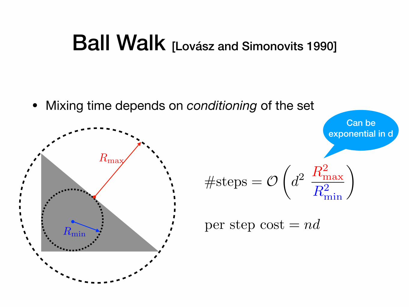
Ball Walk [Lovász and Simonovits 1990]

• Mixing time depends on conditioning of the set

Rmin

Rmax

#steps = O

✓d2

R2max

R2min

◆

per step cost = nd

Can be exponential in d

May be a variable shape ellipsoid?

z

z

• Proposal

• Another variant

• Accept Reject:

Dikin Walk [Kannan and Narayanan 2012]

z

z

z ⇠ N✓x,

r2

dD�1

x

◆

P( accept z) = min

⇢1,

P (z ! x)

P (x ! z)

�

z ⇠ U [Dx(r)]

• Proposal

Dikin Walk [Kannan and Narayanan 2012]

z

zDx =

nX

i=1

aia>i(bi � a>i x)

2

A =

2

6664

—a>1 ——a>2 —

...—a>n—

3

7775K =

�x 2 Rd|Ax b

Log Barrier Method (Optimization)

[Dikin 1967, Nemirovski 1990]

z ⇠ N✓x,

r2

dD�1

x

◆

Upper bounds

Ball Walk Dikin Walk ? ?

#Steps

Per Step Cost

nd

nd

n = #constraints d = #dimensions

n > dnd2

d2R2

max

R2min

Slow mixing of Dikin Walk

�1.0 �0.5 0.0 0.5 1.0�1.0

�0.5

0.0

0.5

1.0

Dikin

�1.0 �0.5 0.0 0.5 1.0�1.0

�0.5

0.0

0.5

1.0

Dikin

#constraints = 128#constraints = 4

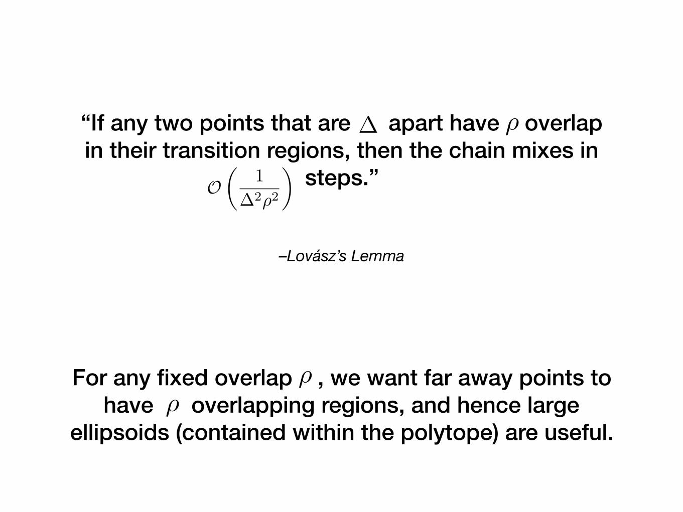
–Lovász’s Lemma

“If any two points that are apart have overlap in their transition regions, then the chain mixes in

steps.”

�

(Distance and overlap measured in appropriately)

⇢

O

✓1

�2⇢2

◆

–Lovász’s Lemma

“If any two points that are apart have overlap in their transition regions, then the chain mixes in

steps.”

� ⇢

O

✓1

�2⇢2

◆

For any fixed overlap , we want far away points to have overlapping regions, and hence large

ellipsoids (contained within the polytope) are useful.

⇢⇢

Improving Dikin Walk

Dikin Proposal

z ⇠ N✓x,

r2

dD�1

x

◆

Dx =nX

i=1

aia>i(bi � a>i x)

2

nX

i=1

wi(x)aia>i

(bi � a>i x)2

Importance weighting of constraints

Log Barrier Method [Dikin 1967, Nemirovski 1990]

Dikin Proposal

z ⇠ N✓x,

r2

dD�1

x

◆

Dx =nX

i=1

aia>i(bi � a>i x)

2

[Kannan and Narayanan 2012]

Improving Dikin Walk

Sampling meets optimization (again!!)

Volumetric Barrier Method [Vaidya 1993]

[Chen, D., Wainwright and Yu 2017]

Log Barrier Method [Dikin 1967, Nemirovski 1990]

Dikin Proposal

z ⇠ N✓x,

r2

dD�1

x

◆

Dx =nX

i=1

aia>i(bi � a>i x)

2

[Kannan and Narayanan 2012]

Vaidya Proposal

z ⇠ N✓x,

r2pnd

V �1x

◆

Vx =nX

i=1

✓�x,i +

d

n

◆aia>i

(bi � a>i x)2

�x,i =a>i D

�1x ai

(bi � a>i x)2

Vaidya Walk [Chen, D., Wainwright, Yu 2017]

#constraints = 128#constraints = 4

�1.0 �0.5 0.0 0.5 1.0�1.0

�0.5

0.0

0.5

1.0

Dikin

Vaidya

�1.0 �0.5 0.0 0.5 1.0�1.0

�0.5

0.0

0.5

1.0

Dikin

Vaidya

Convergence Rates

Ball Walk Dikin Walk

Vaidya Walk

#Steps

Per Step Cost

n0.5d1.5nd

n constraints d dimensions

n > d

d2R2

max

R2min

Convergence Rates

Ball Walk Dikin Walk

Vaidya Walk

#Steps

Per Step Cost

n0.5d1.5nd

ndn constraints d dimensions

n > dnd2

d2R2

max

R2min

nd2

/ n0.45

�1.0 �0.5 0.0 0.5 1.0�1.0

�0.5

0.0

0.5

1.0

initial

�1.0 �0.5 0.0 0.5 1.0�1.0

�0.5

0.0

0.5

1.0

target

Dikin Walk vs Vaidya Walk

k = 0 k = 1

k = #iterations#experiments = 200#dimensions = 2

Dikin Walk

Vaidya Walk

k=10 k=100 k=500 k=1000

Dikin Walk vs Vaidya Walkk = #iterations#experiments = 200#constraints = 64

Dikin Walk

Vaidya Walk

k=10 k=100 k=500 k=1000

Dikin Walk vs Vaidya Walkk = #iterations#experiments = 200#constraints = 64

Dikin Walk

Vaidya Walk

k=10 k=100 k=500 k=1000

Dikin Walk vs Vaidya Walkk = #iterations#experiments = 200#constraints = 64

Dikin Walk

Vaidya Walk

k=10 k=100 k=500 k=1000

Small number of constraints: No Winner!

k = #iterations#experiments = 200#constraints = 64

Dikin Walk

Vaidya Walk

Dikin Walk vs Vaidya Walkk = #iterations#experiments = 200#constraints = 2048

k=10 k=100 k=500 k=1000

Dikin Walk

Vaidya Walk

Dikin Walk vs Vaidya Walkk = #iterations#experiments = 200#constraints = 2048

k=10 k=100 k=500 k=1000

Dikin Walk

Vaidya Walk

Dikin Walk vs Vaidya Walkk = #iterations#experiments = 200#constraints = 2048

k=10 k=100 k=500 k=1000

Dikin Walk

Vaidya Walk

Vaidya walk wins!k = #iterations#experiments = 200#constraints = 2048

k=10 k=100 k=500 k=1000

Dikin Walk vs Vaidya Walk/ n0.9

/ n0.45

O(nd) O(n0.5d1.5)

101 102 103

n

101

102

103

k̂ mix

Dikin

Vaidya / n0.9

/ n0.45

#constraints (n)

vs

Approx. Mixing Time

Polytope approximation to Circle

#constraints = 5 #constraints = 8

Dikin Walk

Vaidya Walk

k=0 k=10 k=100 k=500 k=1000

#constraints = 64

Dikin Walk

Vaidya Walk

k=0 k=10 k=100 k=500 k=1000

Dikin Walk

Vaidya Walk

#constraints = 64

#constraints = 2048

k=0 k=10 k=100 k=500 k=1000

Can we improve further?

Log Barrier Method [Dikin 1967, Nemeirovski 1990]

Vaidya’s Volumetric Barrier Method

[Vaidya 1993]

Dikin Proposal

z ⇠ N✓x,

r2

dD�1

x

◆

Dx =nX

i=1

aia>i(bi � a>i x)

2

Vaidya Proposal

z ⇠ N✓x,

r2pnd

V �1x

◆

Vx =nX

i=1

✓�x,i +

d

n

◆aia>i

(bi � a>i x)2

�x,i =a>i D

�1x ai

(bi � a>i x)2

[Kannan and Narayanan, 2012]

John Walk

Log Barrier Method [Dikin 1967, Nemirovski 1990]

Vaidya’s Volumetric Barrier Method

[Vaidya 1993]

Dikin Proposal

z ⇠ N✓x,

r2

dD�1

x

◆

Dx =nX

i=1

aia>i(bi � a>i x)

2

Vaidya Proposal

z ⇠ N✓x,

r2pnd

V �1x

◆

Vx =nX

i=1

✓�x,i +

d

n

◆aia>i

(bi � a>i x)2

�x,i =a>i D

�1x ai

(bi � a>i x)2

John Proposal

z ⇠ N✓x,

r2

d1.5J�1x

◆

Jx =nX

i=1

jx,iaia>i

(bi � a>i x)2

jx,i = convex program

[Chen, D., Wainwright, Yu 2017][Kannan and Narayanan, 2012]

John’s Ellipsoidal Algorithm

[Fritz John 1948, Lee and Sidford 2015]

Mixing Times

Dikin Walk Vaidya Walk John Walk

#Steps

Per Step Cost

n0.5d1.5nd

n = #constraints d = #dimensions

n > d

d2.5 log4n

d

Mixing Times

Dikin Walk Vaidya Walk John Walk

#Steps

Per Step Cost

n0.5d1.5nd

n = #constraints d = #dimensions

n > d

d2.5 log4n

d

nd2 nd2 nd2 log2 n

Conjecture

Dikin Walk Vaidya Walk John Walk

#Steps

Per Step Cost

n0.5d1.5nd

n = #constraints d = #dimensions

n > d

nd2 nd2 nd2 log2 n

d2 logc⇣nd

⌘

– Numerical Experiments

“ For the John walk, the log factors are bottleneck in

practice. ’’

Proof Idea

• Proof relies on Lovasz’s Lemma

• Need to establish that near by points have similar transition distributions

• Have to show that the weighted matrices are sufficiently smooth — use of weights makes it involved

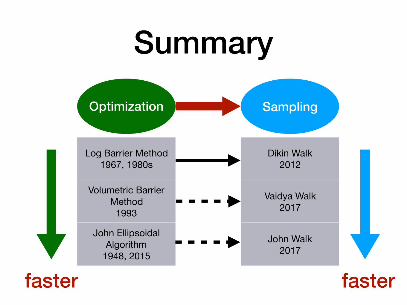
Summary

Optimization Sampling

Log Barrier Method1967, 1980s

Dikin Walk2012

Volumetric Barrier Method

1993

Vaidya Walk2017

John Ellipsoidal Algorithm

1948, 2015

John Walk2017

faster faster