1. INTRODUCTIONMany modern optical systems violate the validity condi-tion for the geometrical-optics approximation (wavelengthsmall with respect to aperture) and must be analyzedwith physical optics propagation (POP) methods (for ex-ample, spatial-filtering systems). Since the developmentof high-numerical-aperture (NA) diode lasers and otherplanar optics waveguides, it has become increasingly im-portant to apply POP to high-aperture, diverging or con-verging, beams, which depart from the paraxial approxi-mation. Many optical systems for coupling high-NAbeams emitted from planar waveguides to fiberwaveguides, and vice versa, have been described.1,2
The motivation for this study was the need to model anoptical system developed at our laboratory, designed to re-lay light emitted from a channel waveguide array to anoutput fiber array,3 where, between the two arrays, a va-riety of lenses of different numerical apertures and sizesare located. Such a system combines portions that canbe described by geometrical-optics methods with portionsnear the source and image planes, where physical opticsgovern the behavior of the optical power distribution. Wefound that commercially available simulation packagesthat have the capability of simulating such a system wereeither limited to paraxial beams or very cumbersome andexpensive.
The paraxial limitation found in most simulation pack-ages is a result of using the Fresnel approximation. Theadvantage of the Fresnel approximation is that it allowsfast numerical computation through use of the fast Fou-rier transform (FFT) algorithm. The purpose of this pa-per is to present an alternative to the classic Fresnelpropagation that is not limited to paraxial beams. LikeFresnel propagation, this propagation method is based ona single Fourier transform, thus offering the same calcu-lation speed. The method can provide the basis for a
simple and fast POP algorithm, which is not limited toparaxial beams. In a previous paper4 this method wasapplied to the analysis of the optical system describedabove and led to the discovery and explanation of a novelphysical phenomenon that could not be simulated withinthe framework of the Fresnel approximation.
The paper is constructed as follows. In Section 2 wepresent background on current Fourier-optics-basedpropagation schemes. In Section 3 we derive the pro-posed integrated propagator, which can replace Fresnelpropagation in the case of diverging beams, lifting theparaxial limitation. A discussion of converging beams isalso included, for the sake of completeness. In Section 4the validity limits of the proposed propagation methodsare explored. In Section 5 the validity of the scalar ap-proximation for the case of a high-NA diverging beam isexamined. In Section 6 simulation and measured resultssupporting the conclusions of the previous sections arepresented.
2. BACKGROUNDIn this section some background will be given regardingthe classic Fourier-optics wave-front propagation meth-ods: angular spectrum and Fresnel. The propagationalgorithm devised by Lawrence,5 based on these twomethods, will also be described.
POP can be divided into two parts: propagation withinhomogeneous media and transfer between different me-dia. This paper will discuss POP of high-NA beams, fo-cusing on the first part and leaving the second part for fu-ture study. Assuming the boundary conditions areknown, a scalar analysis performed on each of the fieldcomponents can give accurate results for propagationwithin homogeneous media. We therefore limit this pa-per to scalar analysis. If the boundary conditions are not
2004 Optical Society of America
2136 J. Opt. Soc. Am. A/Vol. 21, No. 11 /November 2004 Y. M. Engelberg and S. Ruschin
accurately known, Kirchhoff boundary conditions are gen-erally assumed, which leads to some error in the calcu-lated fields (see Section 5).
For propagation in homogeneous media, two basicpropagation methods are used: spatial diffraction inte-gral propagation and angular spectrum propagation.5,6
The two methods are mathematically equivalent (via Fou-rier transform): Angular spectrum propagation relies onsuperposition of plane waves, and diffraction integralpropagation relies on superposition of spherical or para-bolic waves. For diffraction integral propagation, theoriginal wave front is multiplied by a spherical wave func-tion, which we call a propagator, and then the integral isperformed. In the Fresnel (paraxial) approximation thespherical wave is replaced by a parabolic wave, allowingthe integral to take on the form of a Fourier transform.In angular spectrum propagation, equivalent sphericaland parabolic propagators exist, which are Fourier trans-forms of the diffraction integral propagators. Angularspectrum propagation is then performed via two Fouriertransform operations (see Subsection 2.A).
A. Angular Spectrum PropagationAngular spectrum propagation is performed accordingto5,6
a~x, y, z ! 5 FF21$T~z !FF@a~x, y, 0!#%. (1)
a(x, y, 0) and a(x, y, z) are the complex wave-front am-plitudes at the input and output planes, respectively. FFand FF21 symbolize the Fourier and inverse Fouriertransform, respectively, z is the propagation distance, andx, y are the input and output plane coordinates. The ac-curate spherical propagator T(z) is given by
T~z ! 5 exp$ jkz@1 2 ~lj!2 2 ~lh!2#1/2%, (2)
where j, h are spatial-frequency coordinates in the x and ydirections, respectively, obtained from the Fourier trans-form. k 5 2p/l, l being the wavelength. In theFresnel (paraxial) approximation the parabolic propaga-tor is obtained:
Tp~z ! 5 exp~ jkz !exp~2jplzr2!, r2 5 h2 1 j2.(3)
B. Fresnel PropagationFresnel propagation is performed according to5
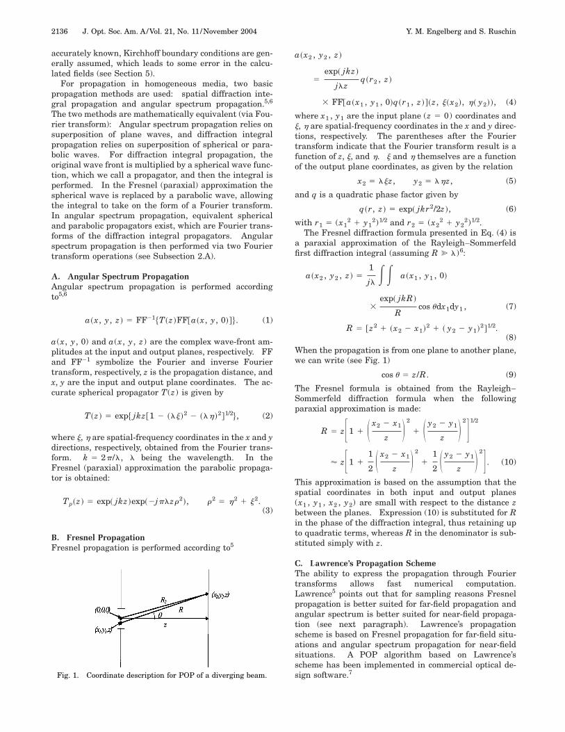
Fig. 1. Coordinate description for POP of a diverging beam.
where x1 , y1 are the input plane (z 5 0) coordinates andj, h are spatial-frequency coordinates in the x and y direc-tions, respectively. The parentheses after the Fouriertransform indicate that the Fourier transform result is afunction of z, j, and h. j and h themselves are a functionof the output plane coordinates, as given by the relation
x2 5 ljz, y2 5 lhz, (5)
and q is a quadratic phase factor given by
q~r, z ! 5 exp~ jkr2/2z !, (6)
with r1 5 (x12 1 y1
2)1/2 and r2 5 (x22 1 y2
2)1/2.The Fresnel diffraction formula presented in Eq. (4) is
a paraxial approximation of the Rayleigh–Sommerfeldfirst diffraction integral (assuming R @ l)6:
a~x2 , y2 , z ! 51
jlEE a~x1 , y1 , 0!
3exp~ jkR !
Rcos udx1dy1 , (7)
R 5 @z2 1 ~x2 2 x1!2 1 ~ y2 2 y1!2#1/2.(8)
When the propagation is from one plane to another plane,we can write (see Fig. 1)
cos u 5 z/R. (9)
The Fresnel formula is obtained from the Rayleigh–Sommerfeld diffraction formula when the followingparaxial approximation is made:
R 5 zF1 1 S x2 2 x1
z D 2
1 S y2 2 y1
z D 2G1/2
' zF1 11
2 S x2 2 x1
z D 2
11
2 S y2 2 y1
z D 2G . (10)
This approximation is based on the assumption that thespatial coordinates in both input and output planes(x1 , y1 , x2 , y2) are small with respect to the distance zbetween the planes. Expression (10) is substituted for Rin the phase of the diffraction integral, thus retaining upto quadratic terms, whereas R in the denominator is sub-stituted simply with z.
C. Lawrence’s Propagation SchemeThe ability to express the propagation through Fouriertransforms allows fast numerical computation.Lawrence5 points out that for sampling reasons Fresnelpropagation is better suited for far-field propagation andangular spectrum is better suited for near-field propaga-tion (see next paragraph). Lawrence’s propagationscheme is based on Fresnel propagation for far-field situ-ations and angular spectrum propagation for near-fieldsituations. A POP algorithm based on Lawrence’sscheme has been implemented in commercial optical de-sign software.7
Y. M. Engelberg and S. Ruschin Vol. 21, No. 11 /November 2004 /J. Opt. Soc. Am. A 2137
The sampling considerations expressed by Lawrenceare as follows. Fresnel propagation is suited for far-fieldnumerical calculations because the quadratic phase factorq in the Fourier transform of Eq. (4) is slow varying as afunction of r1 , for a large propagation distance z [see Eq.(6)]. Therefore dense sampling in the input plane is notrequired. In contrast, the angular spectrum propagatorof Eqs. (2) and (3) varies more rapidly the larger thepropagation distance z. Dense sampling in the frequencydomain is required for large propagation distances, and,as a result, an equal number of samples in the spatial do-main is required. Angular spectrum is therefore bettersuited for near-field propagation.
In summary, the formulas described by Lawrence re-duce computation time by permitting use of the fast Fou-rier transform (FFT) algorithm, instead of point-by-pointnumerical calculation of the diffraction integral. Theprice paid is that the propagation algorithm is limited tothe Fresnel (or the paraxial) approximation.
D. Previous ResearchSteane and Rutt8 and Sheppard and Hrynevych9 sug-gested expanding the validity of the Fresnel approxima-tion by using a corrected Fresnel number. These meth-ods are limited to the near-field or geometricallyilluminated region and are therefore not appropriate forhigh-NA diverging beams, where the shadow region is ofinterest.
Methods have been described to increase the accuracyof POP based on the Fresnel approximation by expandingthe accurate diffraction integral result into a power seriesin a variable proportional to the NA, with the zero ordercorresponding to the Fresnel solution and the higher or-ders corresponding to corrections to the Fresnelsolution.10,11 These corrections are expressed in terms ofthe zero-order Fresnel solution but require calculation ofderivatives of this solution in the direction of propagation,thus not facilitating fast numerical computation.
Forbes et al.12 developed an algebraic correction for theFresnel approximation that does not require calculationof derivatives. The approach taken was one of erroranalysis, based on development of the angular spectrumexpression into a power series. The expression obtainedby Forbes et al. has features similar to that presented inthis paper, but it is more complex and contains an empiricfactor. In this paper a direct approach based on approxi-mation of the diffraction integral is taken. The advan-tages of the method presented here are mathematicalsimplicity and a closed final expression (no empirical fac-tor). This approach does not facilitate analytic erroranalysis but does permit determination of validity limits(see Section 4), which are of practical concern.
3. EXPANSION OF HOMOGENEOUS MEDIAPROPAGATION METHODS TO HIGHNUMERICAL APERTUREIn this section we present an alternative to Fresnel propa-gation, which will allow generalization of Lawrence’spropagation scheme to nonparaxial beams while retain-ing computation speed. The scheme described byLawrence5 uses the paraxial propagator of Eq. (3) for an-
gular spectrum propagation. However, the accuratepropagator of Eq. (2) can be used, without any increase inalgorithm complexity. In addition, if the angular spec-trum propagator is used only for near-field propagation,the paraxial (parabolic) propagator will not give a largeerror. This is because the Fresnel approximation worksbetter in the near field6,13 than anticipated by the phasecondition presented in Subsection 4.A. For these rea-sons, we will focus on extending and modifying Fresnelpropagation to allow simulation of high-NA beams in thefar field.
Three conditions must be fulfilled by a good POP for-mula for numerical simulation purposes: accuracy (noapproximations inappropriate for the specific physicalsituation), speed (FFT-based formula), and low sampling,i.e., computer memory, requirements (no rapidly varyingphase within the FFT). The intention of this section is topresent a method aimed at improving the accuracy of thecustomary Fresnel propagation, with minimal or no dam-age to speed and sampling.
A. High-Numerical-Aperture PropagatorTo obtain a propagator suited for a highly diverging beam,we must avoid the approximation of output spatial coor-dinates small relative to z and implement the approxima-tion only for the input plane spatial coordinates. Thiscan be done approximating R, defined in Eq. (8), in the fol-lowing manner (see Fig. 1):
R 5 R2S 1 1x1
2 2 2x1x2
R22
1y1
2 2 2y1y2
R22 D 1/2
' R2S 1 2x1x2
R22
2y1y2
R22 D , (11)
R2 5 ~z2 1 x22 1 y2
2!1/2. (12)
Here no approximation has been made on the outputplane coordinates (x2 , y2), but a stronger approximationhas been made on the input plane coordinates (x1 , y1).Although in the Fresnel approximation quadratic termswere retained, here quadratic terms in (x1 , y1) were ne-glected, leaving only linear terms. In other words, aFraunhofer-type approximation has been made on the in-put plane coordinates only. This approximation is wellsuited for a high-NA diverging beam in the far field,where the input aperture is small and the output aper-ture is large.
Substituting expression (11) for R in the phase of Eq.(7) and simply R2 for R in the denominator, we can writethe approximated Rayleigh–Sommerfeld diffraction for-mula as
Expression (11) is an alternative to the approximation ofR performed in expression (10). This form of approxima-tion was used by Born and Wolf.14 Zeng et al.15 showed
2138 J. Opt. Soc. Am. A/Vol. 21, No. 11 /November 2004 Y. M. Engelberg and S. Ruschin
that this form of approximation can lead to a Fouriertransform expression, as in Eq. (13). They applied thismethod to finding an analytic expression for the propaga-tion of a high-NA diverging Gaussian beam. In this pa-per we expand this idea methodically for the computationof more general fields encountered in practical systems.
With the high-NA propagation formula of Eqs. (13) and(14), general high-NA diverging beams can be numeri-cally propagated accurately and simply. The only factorthat makes the above formula more complex to imple-ment than Fresnel propagation is that R2 itself is a func-tion of the output coordinates x2 , y2 . Substituting Eq.(12) into Eqs. (14) and solving for x2 , y2 , we obtain
x2 5ljz
@1 2 l2~j2 1 h2!#1/2,
y2 5lhz
@1 2 l2~j2 1 h2!#1/2. (15)
This coordinate transformation is more complex than thelinear transformation of Eqs. (5). For low-NA beams, thespatial frequencies j and h, at which there is significantpower, are small, so the coordinate transformation degen-erates back into Eqs. (5). For high-NA beams, there iscoupling between the spatial frequencies in the two direc-tions to form the correct output coordinates. This cou-pling is important in describing certain high-NA diffrac-tion phenomena in asymmetric systems that are lostwhen the more restricted Fresnel transformation isperformed.4
As mentioned, the output spatial coordinates are nolonger linear with respect to the spatial-frequency coordi-nates. Therefore, if it is necessary to perform an addi-tional propagation step, the output array must be resa-mpled in equal intervals, by use of interpolation. Theresampling can be done for output coordinate points de-fined by the linear transformation of Eqs. (5). The inter-polation introduces a speed penalty; however, it is fasterby orders of magnitude than performing the explicitpoint-by-point diffraction integral. Otherwise, thehigh-NA propagation introduced in Eq. (13) has formalsimilarity to Fraunhofer’s diffraction formula, and all thewell-known properties of Fraunhofer’s calculations, foundin textbooks, can be translated into the more general caseof high-NA propagation that was introduced here. Inconclusion, the nonlinearity and coordinate-couplingproperty are located in the relationship between the coor-dinates in the Fourier space and the regular space. Boththese properties are of relevance at high NAs and are lostin the Fresnel approximation.
B. Integrated PropagatorFrom Subsection 3.A it is clear that the Fresnel propaga-tor is suited for low-NA far-field propagation and thehigh-NA propagator is suited for high-NA far-field propa-gation. The exact validity limits of these propagationmethods are discussed in Section 4. For the time being,an intuitive approach will be used. The Fresnel propa-gator is not accurate for high-NA diverging beams mainlybecause the phase factor in x2 , y2 outside the Fouriertransform is parabolic instead of spherical. On the other
hand, the high-NA propagator is valid only if the Fraun-hofer approximation holds because the quadratic phasefactor in x1 , y1 was neglected. For low NA (aperture notso small), the distance at which the Fraunhofer approxi-mation holds will be large (since for Fraunhofer the dis-tance must be much greater than the aperture, so thateven the quadratic terms are neglected), thus limiting thevalidity of the high-NA propagation algorithm.
At this point it must be clarified what is meant by theexpression ‘‘far field.’’ Generally the term is used for dis-tances from the diffracting aperture at which the Fraun-hofer approximation holds.16 In this sense, the high-NApropagator suggested in Subsection 3.A can be said to bevalid for all far-field cases. In most physical optics simu-lation packages, angular spectrum propagation is used forthe near field and Fresnel propagation for the far field.In Zemax optical design software, the switchover pointbetween algorithms is set to twice the Rayleigh distance(of a Gaussian beam that best fits the actual wave front).7
This distance is considered far field for simulation pur-poses, although it is not far field in the original sense. Atsuch a distance the Fraunhofer approximation is notvalid, and the Fresnel approximation must be used.Therefore the high-NA propagation algorithm of Subsec-tion 3.A cannot fully replace the Fresnel propagation al-gorithm in all cases of physical optics simulations. In thefollowing an integrated propagator is presented that canfully replace the Fresnel propagator, giving accurate re-sults for the full range of NAs.
The most significant phase factor neglected in expres-sion (11) was a quadratic of the form: (x1
2 1 y12)/2R2 .
A diffraction formula that does not neglect this factor isgiven by Forbes.17 However, since R2 is not a constantbut rather a function of (x2 , y2), retaining this factordoes not result in a Fourier-transform-like expression.We postulate that a good approximation of that factor canbe obtained by replacing R2 with z. This is a result of thefollowing consideration: If x1 , y1 are small, as in thehigh-NA case, the entire quadratic phase factor is negli-gible. If, on the other hand, x1 , y1 are not so small, thenx2 , y2 will not be so large, since the diffraction angle willbe small, and z will be a reasonable approximation of R2 .
An integrated far-field propagator suitable for the fullrange of NAs can therefore be obtained by adding theFresnel quadratic phase factor of Eq. (6) into the high-NApropagation formula of Eq. (13):
with q, R2 , and x2 , y2 as defined in Eqs. (6), (12), and(15), respectively. Note that this expression is nearlyidentical to the Fresnel propagation formula of Eq. (4).The main differences are use of the coordinate transfor-mations (15) instead of Eqs. (5) and use of a spherical, in-stead of parabolic, image-plane phase factor. Thehigh-NA propagator may be regarded as a didactic step onthe way to the more general integrated propagator, which
Y. M. Engelberg and S. Ruschin Vol. 21, No. 11 /November 2004 /J. Opt. Soc. Am. A 2139
can be used as the sole far-field propagation algorithm, re-placing both Fresnel and high-NA propagation.
C. High-Numerical-Aperture Converging BeamFor a converging beam, one can take an approach similarto that used with the diverging beam, this time makingthe approximation that the output coordinates are smallwith respect to the propagation distance z. However, thiswill not produce a simple Fourier-transform-based for-mula, as with the diverging beam. This is because thediffraction integral is over the input plane coordinates.Therefore the simplification of the integral into a Fouriertransform is obtained only if the input plane coordinatesare small.
It would therefore appear that for the case of a high-NAconverging beam there is no alternative to performing afull diffraction integral. However, this is the case only ifit is required to propagate the wave front from one planeto another. If the input converging wave front is definedrelative to a reference sphere, as shown in Fig. 2, then asimple expression for the propagation can again be ob-tained.
The standard Fresnel–Kirchhoff6 and Rayleigh–Sommerfeld [Eq. (7)] diffraction integrals are based onthe assumption of a reference plane, not a referencesphere. However, the Fresnel–Kirchhoff integral is cor-rect also for a spherical reference, provided that the cor-rect inclination factor is used.14 For the case of a con-verging wave that produces a small spot size and areference sphere centered near the spot centroid, the in-clination factor can be approximated as 1. The Fresnel–Kirchoff diffraction integral then takes the form of Eq. (7),with cos u ' 1.
Starting from the modified Eq. (7), with x1 , y1 now thecoordinates on the reference sphere, the following ap-proximation, parallel to expression (11), can be made:
R 5 zS 1 1x2
2 2 2x1x2
z21
y22 2 2y1y2
z2 D 1/2
' zS 1 1x2
2 1 y22
2z22
x1x2
z22
y1y2
z2 D ,
z 5 ~z12 1 x1
2 1 y12!1/2 5 const. (17)
Substituting expression (17) into the modified Eq. (7), weobtain
Fig. 2. Coordinate description for POP of a converging beam.
a~x2 , y2 , 0! 5exp~ jkz !
jlzq~r2 , z !
3 FF@a~x1 , y1!#~j~x2!, h~ y2!!. (18)
The coordinate transformation is given by Eqs. (5).Equation (18) is exactly the expression of Fraunhoferdiffraction.6 In other words, for the case of a nearlyspherical converging beam, defined on a reference sphere,a new propagator is not needed, since Fraunhofer is accu-rate. This well-known fact provides the basis for themethod used in commercial optical design software tocompute the point-spread function of optical systems atthe image plane.
4. VALIDITY LIMIT OF PROPAGATORSA. Fresnel PropagatorThe validity limit for Fresnel propagation, based on thephase terms neglected in expression (10), is given inGoodman’s textbook6:
p
4lz3@~x2 2 x1!2 1 ~ y2 2 y1!2#2 ! 1. (19)
Goodman goes on to explain that this expression is overlypessimistic in the near field. However, for the far field itis accurate, and this is our present concern.
For our analysis we can simplify the condition of ex-pression (19) by looking at two-dimensional (2D) propaga-tion (in the XZ plane) and limiting the magnitude of theoutput plane coordinate x2 , in the phase condition of ex-pression (19), to the range in which there is significant in-tensity (where there is no intensity, the phase error willhave no effect). This range can be estimated on the basisof the paraxial far-field diffraction pattern of a slit (i.e.,assuming a plane wave with a top-hat intensity incidentbeam). For an aperture with half-width x1max , the inten-sity diffraction pattern will be of sinc2 form, with the firstzero located at16
x2 ~first intensity minimum! 5lz
2x1max. (20)
The maximum x2 of interest can therefore be written as
x2 max 5 blz
x1max, (21)
where b is a constant that determines the level of inten-sity for which phase error is still considered important.If b 5 1, it means the output wave front until the seconddiffraction intensity minimum is considered. If the inci-dent wave front is fairly smooth and mostly limited to anaperture of x1max but departs from the plane-wave top-hatform, this can be accounted for by adjusting the value of b.Substituting x2 max from Eq. (21) for x2 in expression (19),we can write the Fresnel validity condition as
x1max .1
2 H S 0.4lz3
pD 1/4
2 F S 0.4lz3
pD 1/2
2 4blzG1/2J ,
(22)
2140 J. Opt. Soc. Am. A/Vol. 21, No. 11 /November 2004 Y. M. Engelberg and S. Ruschin
where the ‘‘much-smaller-than-1’’ condition of expression(19) was translated to smaller than 0.1. Expression (22)gives a lower bound for the size of the input aperture.Expression (19) implies also a higher bound for the inputaperture. However, this is relevant to the near-field case,whereas our analysis here is limited to the far field (in thesimulation sense, see Subsection 3.B). The lower boundoriginates physically from the fact that too small an aper-ture will result in a large diffraction angle, contradictingparaxiality.
B. High-Numerical-Aperture PropagatorThe validity limit of the high-NA propagator can be ob-tained in a manner similar to the Fresnel validity limit,on the basis of the approximation made in expression (11).The condition, based on the two lowest-level terms ne-glected in the phase expression, is
U p
lR2~x1
2 1 y12! 2
p
4lR23
@x1~x1 2 2x2!
1 y1~ y1 2 2y2!]2U ! 1. (23)
It is immediately evident that for x1 , y1 sufficiently smallwith respect to R2 the high-NA approximation is valid, re-gardless of the magnitude of x2 , y2 .
Again looking at 2D propagation and using Eq. (21), wecan obtain the following validity condition:
x1max , ~lz/10p!1/2. (24)
C. Integrated PropagatorIn the case of the integrated propagator, the quadraticphase factor in x1 , y1 is retained, but R2 is replaced withz. Therefore instead of expression (23) we have
U p
lR2~x1
2 1 y12! 2
p
lz~x1
2 1 y12! 2
p
4lR23
3 @x1~x1 2 2x2! 1 y1~ y1 2 2y2!#2U ! 1. (25)
Making the simplifications of 2D propagation and usingEq. (21), we can obtain the following validity condition:
z .10px1max
2
lUF1 1 S bl
x1maxD 2G23/2
2 1U. (26)
For x1 ! l, expression (26) degenerates into expression(24). For x1 @ l, the condition becomes
z . 15pb2l, (27)
independent of input aperture size.
D. Converging BeamFor the case of a converging beam, both the standardFresnel approximation (see Goodman6) and the high-NAapproximation (see Subsection 3.C) reduce to the Fraun-hofer form. To analyze the validity limit of the high-NAapproximation, we look at the lowest-level terms ne-glected in expression (17) and obtain the requirement
p
4lz3@x2~x2 2 2x1! 1 y2~ y2 2 2y1!#2 ! 1. (28)
Making the simplifications of 2D propagation, we are ledto the conclusion that the Fraunhofer approximation isvalid at the focus of a converging beam, as long as
x2max , 0.6~lz3!1/4. (29)
This means that for a diffraction-limited system theFraunhofer approximation is valid at the focus, at an ar-bitrarily high output NA, limited only by the scalar ap-proximation. (There is an upper limit on aperture sizeintroduced by inaccuracy of the Sommerfeld diffractionintegral for converging beams,18 but this is beyond thescope of this paper.) However, expression (29) imposes alower limit on the NA for which Fraunhofer will be accu-rate. By use of Eq. (21), the condition on the NA is
NA . 1.67b~l/z !3/4. (30)
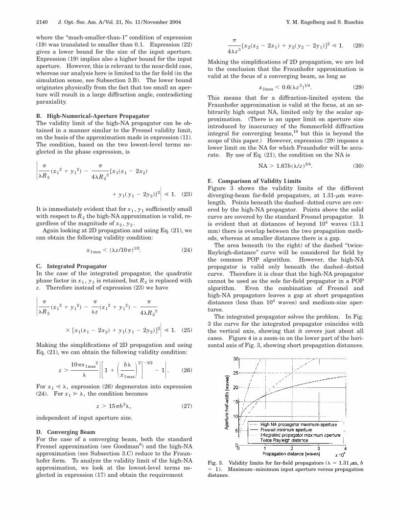
E. Comparison of Validity LimitsFigure 3 shows the validity limits of the differentdiverging-beam far-field propagators, at 1.31-mm wave-length. Points beneath the dashed–dotted curve are cov-ered by the high-NA propagator. Points above the solidcurve are covered by the standard Fresnel propagator. Itis evident that at distances of beyond 104 waves (13.1mm) there is overlap between the two propagation meth-ods, whereas at smaller distances there is a gap.
The area beneath (to the right) of the dashed ‘‘twice-Rayleigh-distance’’ curve will be considered far field bythe common POP algorithm. However, the high-NApropagator is valid only beneath the dashed–dottedcurve. Therefore it is clear that the high-NA propagatorcannot be used as the sole far-field propagator in a POPalgorithm. Even the combination of Fresnel andhigh-NA propagators leaves a gap at short propagationdistances (less than 104 waves) and medium-size aper-tures.
The integrated propagator solves the problem. In Fig.3 the curve for the integrated propagator coincides withthe vertical axis, showing that it covers just about allcases. Figure 4 is a zoom-in on the lower part of the hori-zontal axis of Fig. 3, showing short propagation distances.
Fig. 3. Validity limits for far-field propagators (l 5 1.31 mm, b5 1). Maximum–minimum input aperture versus propagationdistance.
Y. M. Engelberg and S. Ruschin Vol. 21, No. 11 /November 2004 /J. Opt. Soc. Am. A 2141
From this graph it can be seen that for propagation dis-tances larger than 48 waves the integrated propagator isaccurate for any aperture size, limited only by a weak far-field requirement, necessary for validity of the estimate ofEq. (21). For shorter propagation distances there is astronger far-field requirement, which matches the twice-Rayleigh-distance criterion fairly well. As a final com-ment, we note that all the approaches presented here re-main within the framework of the scalar approximationand cannot account for aperture-edge and polarization ef-fects in the vicinity of the aperture. Some of these limi-tations are discussed in Section 5.
5. VALIDITY OF SCALAR APPROXIMATIONFOR A HIGH-NUMERICAL-APERTUREDIVERGING BEAMThe propagation of a monochromatic electromagneticwave in linear, isotropic, and homogeneous media can beaccurately described by the well-known scalar waveequation14
¹2E 2n2
c2
]2E
]t25 0. (31)
E is the electric field vector (a similar equation can bewritten for the magnetic field), n is the media refractiveindex, and c is the speed of light in vaccum. This equa-tion can be separated into three wave equations, for eachof the components of E, since there is no coupling betweencomponents in the above equation.
However, generally our interest does not begin and endwith wave propagation in homogeneous media. The elec-tromagnetic wave generally comes from a light source (forexample, a slit illuminated by a laser beam) and, only onexiting it, begins to propagate in homogeneous media.The approximation of the scalar analysis comes from theboundary conditions used with the wave equation. Theboundary conditions usually applied are the Kirchhoffboundary conditions19:
1. Within the illuminated aperture, the field distribu-tion a(x, y, z) and its derivative (]a/]z) are the same asin the absence of the aperture.
2. Outside the aperture, both of the above are identi-cally zero.
Fig. 4. Zoom-in on Fig. 3, for small propagation distances.
Although the above boundary conditions cannot beaccurate,19 they give a good approximation if the apertureis large with respect to the wavelength. Since an aper-ture large with respect to wavelength inevitably gives riseto small diffraction angles, the scalar approximation is of-ten equated with the paraxial approximation. This canlead to thinking that there is no point in using an accu-rate diffraction integral for high-NA beam propagation in-stead of the Fresnel diffraction integral, since the bound-ary conditions used with the diffraction integral will limitus to the paraxial region anyway (an estimate of the errorintroduced by the Kirchhoff boundary conditions is givenby Forbes17). However this is not true for several rea-sons. (a) The main error associated with the Fresnel ap-proximation is the parabolic phase instead of the spheri-cal phase, and this is removed, regardless of the exactboundary conditions. (b) Important changes in the inten-sity pattern as a result of coupling effects in nonsymmet-ric beams are lost in the Fresnel approximation but canbe simulated with high-NA propagation.4 (c) In Section 6some results will be shown for calculated versus mea-sured far-field intensity diffraction patterns for a high-NAslit and waveguide, showing that the high-NA propaga-tion method gives intensity pattern results closer to real-ity than the Fresnel approximation (although by nomeans accurate) when Kirchhoff boundary conditions forwavelength-sized slits are used. (d) In the case of lightsources such as semiconductor lasers and waveguideedges radiating into free space, the fields in the vicinity ofthe device are accurately known from the solution of Max-well’s equations in waveguide structures. These fieldshave definite polarizations and can be used as aperturesources for all the approaches presented here. These ex-act fields remove the need of imposing Kirchhoff bound-ary conditions. In that case the scalar approximation isremoved, and the analysis performed in the previous sec-tions is accurate. This accuracy is lost if the Fresnel ap-proximation is used.
On the basis of the above considerations, we concludethat the scalar approximation is much better than theFresnel approximation. Therefore, for practical pur-poses, lifting the paraxial limitation from scalar analysisis of great utility, allowing analysis of modern high-NAoptical systems.
6. RESULTSA. Simulation Results: Diverging High-Numerical-Aperture BeamTo evaluate the behavior of the various propagation meth-ods in the case of a high-NA diverging beam, we modeledthe system shown in Fig. 5. A point source is located atthe focus (4.389 mm left of the first lens surface) of a
Fig. 5. Sample optical system for evaluation of different propa-gation methods.
2142 J. Opt. Soc. Am. A/Vol. 21, No. 11 /November 2004 Y. M. Engelberg and S. Ruschin
6-mm focal-length lens. The lens is plano–convex, withan aspheric convex side, optimized by geometrical-opticsmethods so that the beam is perfectly collimated (negli-gible aberrations with respect to diffraction limit) on ex-iting the lens. In physical optics terms, one can say thatthe lens is optimized to produce a plane wave from an in-cident spherical wave, emitted from the point source.The beam is then focused down by use of a 100-mm focal-length ideal lens.
For physical optics simulation, the point source is re-placed by a Gaussian beam at its waist. The waist ra-dius is 0.75 mm, and the operating wavelength is 1.31 mm.The lens apertures are assumed to be large, so that theydo not introduce significant diffraction effects. First,propagation from the beam waist, a distance of 4.389mm—up to the plano lens surface, will be analyzed.
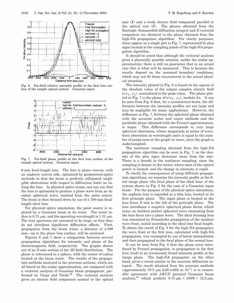
Figures 6 and 7 show a comparison between severalpropagation algorithms for intensity and phase of theelectromagnetic field, respectively. The graphs shownare of an X-axis section of the 2D field distribution. Thephase is referenced to a sphere, with the center of radiuslocated at the beam waist. The results of the propaga-tion methods analyzed in the previous sections, which areall based on the scalar approximation, are compared witha vectorial analysis of Gaussian beam propagation, per-formed by Varga and Torok.20 The vectorial analysisgives an electric field component normal to the optical
Fig. 6. Far-field relative intensity profile at the first lens sur-face of the sample optical system: Gaussian input.
Fig. 7. Far-field phase profile at the first lens surface of thesample optical system: Gaussian input.
axis (X) and a weak electric field component parallel tothe optical axis (Z). The phases obtained from theRayleigh–Sommerfeld diffraction integral and X-vectorialcomponent are identical to the phase obtained from thehigh-NA propagation algorithm. For clarity purposes,these appear as a single plot in Fig. 7, represented by plussigns located at the sampling points of the high-NA propa-gation algorithm.
It should be noted that although the vectorial analysisgives a physically possible solution, unlike the scalar ap-proximation, there is still no guarantee that in an actualcase this is what will be measured. This is because theresults depend on the assumed boundary conditions,which may not fit those encountered in the actual physi-cal situation.
The intensity plotted in Fig. 6 is based on the square ofthe absolute value of the output complex electric fielda(x2 , y2), normalized to the peak value. The phase plot-ted in Fig. 7 is the phase of a(x2 , y2), modulo 2p. It canbe seen from Fig. 6 that, for a symmetrical beam, the dif-ferences between the intensity profiles are not large andmay be negligible for many applications. However, thedifference in Fig. 7, between the spherical phase obtainedwith the accurate scalar and vector methods and theparabolic phase obtained with the Fresnel approximation,is major. This difference corresponds to very largespherical aberration, whose magnitude in terms of wave-front aberration in wavelength units is equal to the num-ber of jumps seen in the graph (or more, since the graph isundersampled).
The nonlinear sampling obtained from the high-NApropagation algorithm can be seen in Fig. 7, as the den-sity of the plus signs decreases away from the axis.There is a benefit in the nonlinear sampling, since thesampling is denser in the center, where most of the opticalpower is located, and the change in intensity is rapid.
To clarify the consequences of using different propaga-tion algorithms, we examine the intensity profile at the fi-nal image plane (the focal plane of the ideal lens) of thesystem shown in Fig. 5 for the case of a Gaussian inputbeam. For the purpose of the physical optics simulation,the aspheric lens is regarded as a thin lens, located at itsfirst principle plane. The input plane is located at thelens focus, 6 mm to the left of the principle plane. Thelens introduces a negative spherical phase factor, whichturns an incident perfect spherical wave emanating fromthe lens focus into a plane wave. The ideal focusing lenswas simulated by Fraunhofer propagation of the incidentwave front, scaled according to the ideal lens focal length.To obtain the result of Fig. 8 for the high-NA propagator,the wave front at the first lens, calculated with high-NApropagation, was resampled by use of linear interpolationand then propagated to the focal plane of the second lens.
It can be seen from Fig. 8 that the phase error intro-duced by Fresnel propagation, in propagation to the firstlens, leads to an erroneously broad intensity profile at theimage plane. The high-NA propagator, on the otherhand, gives a result similar to the accurate diffraction in-tegral. The result obtained from the accurate methods(approximately 10.5 mm half-width at 1/e2) is in reason-able agreement with ABCD paraxial Gaussian beamanalysis,21 which predicts 0.75 mm 3 100/6 5 12.5 mm,
Y. M. Engelberg and S. Ruschin Vol. 21, No. 11 /November 2004 /J. Opt. Soc. Am. A 2143
when both lenses are assumed ‘‘ideal.’’ ‘‘Ideal’’ forparaxial Gaussian beam analysis means the introductionof a quadratic phase to offset the Fresnel quadratic phaseof the beam, so there is no spherical aberration. Al-though this use of ideal lenses corrects the Fresnel phaseerror, it does not correct the intensity profile. This ex-plains the small difference between the accurate image-plane spot size and the paraxial Gaussian beam analysisresult.
B. Simulation Results: Validity LimitsIn this subsection, simulation results for two apertures,at wavelength 1.31 mm and propagation distance of 5000waves, are presented, to validate the analytic expressionsof validity obtained in Section 4 and plotted in Fig. 3.The simulations were done in two dimensions, and the ap-erture used was a slit (top-hat intensity distribution), giv-ing rise to an approximately (in the paraxial approxima-tion) sinc2 shaped far-field intensity distribution. Forthe intermediate-size apertures simulated, the far-fieldintensity distributions calculated by Fresnel approxima-tion, high-NA propagator, and integrated propagator areall fairly accurate and therefore nearly coincide with thefull diffraction integral calculation. Therefore, in thissubsection, the far-field phase only is shown. The phasediscontinuities in the graphs (other than those resultingfrom the modulo 2p) correspond to intensity minima.
In Fig. 9 it can be seen that at a 5-wave half-width ap-
Fig. 8. Focal-plane spot size obtained for the sample optical sys-tem by use of different propagation methods.
Fig. 9. Far-field (distance of 5000 waves) phase distribution fora 5-wave half-width aperture.
erture, the high-NA and integrated propagator results co-incide with the accurate diffraction integral results, allgiving a flat (spherical) phase, while Fresnel propagationgives an erroneous parabolic phase, which departs fromthe spherical reference phase. Figure 10 shows that at a20-wave half-width aperture the Fresnel and integratedpropagator results coincide with the accurate diffractionintegral, whereas the high-NA propagator remains withan erroneous spherical phase. These results correspondwell to Fig. 3. It can be seen that the integrated propa-gator is accurate over the entire region.
C. Measured Results: Scalar Approximation ValidityThe purpose of this subsection is to demonstrate that, forsmall apertures, a more accurate simulation of intensityprofile can be obtained by using high-NA propagation in-stead of Fresnel propagation, even when Kirchhoff bound-ary conditions are used [advantage (c) in Section 5]. Themeasurement reported in this subsection is of a true far-field situation (well within the Fraunhofer region).Therefore the advantage of the integrated propagator isnot revealed in this case, its result being identical to thehigh-NA propagator. The phase of the wave front wasnot measured directly. However, it seems reasonable toassume that the far-field phase of a very small aperture isspherical, regardless of what boundary conditions prevail.
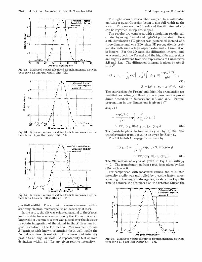
The test setup shown in Fig. 11 was used to measurefar-field intensity of 1.31-mm light diffracted from a slit.The slits used were made of chrome coated on glass. Dif-fraction from two slit widths was measured: 1.75 and 3.5
Fig. 10. Far-field (distance of 5000 waves) phase distribution fora 20-wave half-width aperture.
Fig. 11. Setup for measurement of slit diffraction far-field inten-sity pattern; dia, diameter.
2144 J. Opt. Soc. Am. A/Vol. 21, No. 11 /November 2004 Y. M. Engelberg and S. Ruschin
mm (full width). The slit widths were measured with ascanning electron microscope, to an accuracy of 65%.
In the setup, the slit was oriented parallel to the X axis,and the detector was scanned along the Y axis. A muchlarger slit of 0.5 mm 3 5 mm was placed over the detectorto obtain integration of the signal in the X direction butgood resolution in the Y direction. Measurement at twoZ locations with known separation (both well inside thefar field) allowed translation of the measured intensityprofile to an angular scale. A repeatability test showeddeviations within 61° (for any given relative intensity).
Fig. 12. Measured versus calculated far-field intensity distribu-tions for a 3.5-mm (full-width) slit: TE.
Fig. 13. Measured versus calculated far-field intensity distribu-tions for a 3.5-mm (full-width) slit: TM.
Fig. 14. Measured versus calculated far-field intensity distribu-tions for a 1.75-mm (full-width) slit: TE.
The light source was a fiber coupled to a collimator,emitting a quasi-Gaussian beam 1 mm full width at thewaist. This means the Y profile of the illuminated slitcan be regarded as top-hat shaped.
The results are compared with simulation results cal-culated by using Fresnel and high-NA propagation. Herea 2D simulation (YZ plane) was performed instead of athree-dimensional one (3D) (since 3D propagation is prob-lematic with such a high aspect ratio and 2D simulationis faster). For the 2D case, the diffraction integral and,as a result, both the Fresnel and the high-NA expressionsare slightly different from the expressions of Subsections2.B and 3.A. The diffraction integral is given by (for R@ l)19
a~x2 , z ! 5z
AlexpS 2j
p
4 D E a~x1 , 0!exp~ jkR !
R3/2dx1 ,
(32)
R 5 @z2 1 ~x2 2 x1!2#1/2. (33)
The expressions for Fresnel and high-NA propagation aremodified accordingly, following the approximation proce-dures described in Subsections 2.B and 3.A. Fresnelpropagation in two dimensions is given by19
a~x2 , z !
5exp~ jkz !
AlzexpS 2j
p
4 D q~x2 , z !
3 FF@a~x1 , 0!q~x1 , z !#~z, j~x2!!. (34)
The parabolic phase factors are as given by Eq. (6). Thetransformation from j to x2 is as given by Eqs. (5).
The 2D high-NA propagator is given by
a~x2 , z ! 5z
AlR23
exp~2jp/4!exp~ jkR2!
3 FF@a~x1 , 0!#~z, j~x2!!. (35)
The 2D version of R2 is as given in Eq. (12), with y25 0. The transformation from j to x2 is as given by Eqs.(15), with h 5 0.
For comparison with measured values, the calculatedintensity profile was multiplied by a cosine factor, corre-sponding to the angle of divergence, as shown in Eq. (36).This is because the slit placed on the detector causes the
Fig. 15. Measured versus calculated far-field intensity distribu-tions for a 1.75-mm (full-width) slit: TM.
Y. M. Engelberg and S. Ruschin Vol. 21, No. 11 /November 2004 /J. Opt. Soc. Am. A 2145
detector to measure irradiance on the detector scan plane,whereas the diffraction integral gives irradiance for a sur-face coincident with the wave front (normal to the direc-tion of propagation at every point).
Ioutput plane } ua~x2 , y2 , z !u2 cos u 5 ua~x2 , y2 , z !u2z
R2.
(36)
Figure 12 shows the intensity profile measured withthe above setup, for a slit 3.5 mm wide and for polariza-tion parallel to the slit (TE). Figure 13 shows the samefor polarization normal to the slit (TM). Figures 14 and15 show the same for a 1.75-mm slit. The asymmetricrise in intensity on the right side of the last two figures isprobably a result of background light that got to the de-tector. It can be seen that for the 1.75-mm slit the mea-sured intensity profile is narrower than the predicted pro-file, especially for TE polarization. However, it appearsthat a reasonably good engineering estimate of spot sizecan still be obtained, at an NA of 0.5. It can be seen thatthe measured results match the high-NA propagation re-sults better than the Fresnel results, taking note of thereduced sidelobes. A similar disappearance of sidelobeswas seen in the simulation of diffraction from a small cir-cular aperture.
7. CONCLUSIONSA fast numerical method for far-field wave-front propaga-tion has been presented, which is not limited by theparaxial approximation. This integrated far-field propa-gator can replace Fresnel propagation in physical opticspropagation schemes and still retain its main mathemati-cal advantages, allowing simulation of modern coherenthigh-NA systems.
Use of the integrated propagator instead of the Fresnelpropagator entails a small speed penalty, as a result ofthe need for resampling before the next propagation step.This might be a consideration for favoring the use ofFresnel propagation where it applies and resorting to theintegrated propagator only when necessary. Addition-ally, we have shown by measurement that the scalar ap-proximation is not a serious limiting factor in simulatingmoderately high-NA (at least up to 0.5) optical systems.
The main difference between the integrated far-fieldpropagator and the Fresnel propagator is replacement ofthe quadratic phase in the output plane by the sphericalphase. However, there are additional differences, stem-ming from the different coordinate transformation andamplitude factors outside the Fourier transform. Thesedifferences give rise to the disappearance of the secondarymaxima in slit or top-hat diffraction patterns. More pro-nounced differences in intensity patterns were observedin asymmetrical high-NA beams.4
ACKNOWLEDGMENTSThis work was supported by Chiaro Networks Ltd. in Is-rael. The authors thank Eyal Shekel, Gil Tidhar, DavidBraun, and the other workers at Chiaro for their help.
REFERENCES1. A. Ogura, S. Kuchiki, K. Shiraishi, K. Ohta, and I. Oishi,
‘‘Efficient coupling between laser diodes with a highly ellip-tic field and single-mode fibers by means of GIO fibers,’’IEEE Photonics Technol. Lett. 13, 1191–1193 (2001).
2. M. J. Landry, J. W. Rupert, and A. Mittas, ‘‘Coupling of highpower laser diode optical power,’’ Appl. Opt. 30, 2514–2525(1991).
3. E. Shekel, A. Fiengold, Z. Fradkin, A. Geron, J. Levy, G.Matmon, D. Majer, E. Rafaeli, M. Rudman, G. Tidhar, J.Vecht, and S. Ruschin, ‘‘64 3 64 fast optical switching mod-ule,’’ in Optical Fiber Communication Conference, Vol. 1 of2002 OSA Technical Digest Series (Optical Society ofAmerica, Washington, D.C., 2002), pp. 27–29.
4. Y. M. Engelberg and S. Ruschin, ‘‘Coma aberration in dif-fraction from a narrow slit,’’ in Optical Modeling and Per-formance Predictions, M. A. Kahan, ed., Proc. SPIE 5178,112–123 (2003).
5. G. N. Lawrence, ‘‘Optical modeling,’’ in Applied Optics andOptical Engineering Series, R. R. Shanon and J. C. Wyant,eds. (Academic, San Diego, Calif., 1992), Vol. XI, pp. 125–200.
6. J. W. Goodman, Introduction to Fourier Optics (McGraw-Hill, New York, 1968).
8. A. M. Steane and H. N. Rutt, ‘‘Diffraction calculations inthe near field and the validity of the Fresnel approxima-tion,’’ J. Opt. Soc. Am. A 6, 1809–1814 (1989).
9. C. J. R. Sheppard and M. Hrynevych, ‘‘Diffraction by a cir-cular aperture: a generalization of Fresnel diffractiontheory,’’ J. Opt. Soc. Am. A 9, 274–281 (1992).
10. G. P. Agrawal and M. Lax, ‘‘Free-space wave propagationbeyond the paraxial approximation,’’ Phys. Rev. A 27, 1693–1695 (1983).
11. M. A. Alonso, A. A. Asatryan, and G. W. Forbes, ‘‘Beyond theFresnel approximation for focused waves,’’ J. Opt. Soc. Am.A 16, 1958–1969 (1999).
12. G. W. Forbes, D. J. Butler, R. L. Gordon, and A. A. Asatryan,‘‘Algebraic corrections for paraxial wave fields,’’ J. Opt. Soc.Am. A 14, 3300–3315 (1997).
13. W. H. Southwell, ‘‘Validity of the Fresnel approximation inthe near field,’’ J. Opt. Soc. Am. 71, 7–14 (1981).
14. M. Born and E. Wolf, Principles of Optics (Pergamon, NewYork, 1964).
15. X. Zeng, C. Liang, and Y. An, ‘‘Far-field radiation of planarGaussian sources and comparison with solutions based onthe parabolic approximation,’’ Appl. Opt. 36, 2042–2047(1997).
16. E. Hecht, Optics (Addison-Wesley, Reading, Mass., 1974).17. G. W. Forbes, ‘‘Validity of the Fresnel approximation in the
diffraction of collimated beams,’’ J. Opt. Soc. Am. A 13,1816–1826 (1996).
18. L. Frank, ‘‘The properties of the Sommerfeld diffraction in-tegral for a large aperture converging beam,’’ Optik (Stut-tgart) 43, 149–157 (1975).
19. J. J. Stamnes, Waves in Focal Regions (Hilger, Bristol, UK,1986).
20. P. Varga and P. Torok, ‘‘The Gaussian wave solution of Max-well’s equations and the validity of scalar wave approxima-tion,’’ Opt. Commun. 152, 108–118 (1998).