Fast nonlinear model predictive planner and control for an unmanned ground vehicle in the presence of disturbances and dynamic obstacles Subhan Khan ( [email protected]) University of New South Wales (UNSW) Jose Guivant University of New South Wales (UNSW) Research Article Keywords: nmpc, dynamic, control, vehicle, under, environment, static, obstacles Posted Date: November 18th, 2021 DOI: https://doi.org/10.21203/rs.3.rs-1057351/v1 License: This work is licensed under a Creative Commons Attribution 4.0 International License. Read Full License
Transcript
Fast nonlinear model predictive planner and controlfor an unmanned ground vehicle in the presence ofdisturbances and dynamic obstaclesSubhan Khan ( [email protected] )
This paper presents a solution for the tracking control problem, for an unmanned ground vehicle (UGV), under the presence of
skid-slip and external disturbances in an environment with static and moving obstacles. To achieve the proposed task, we
have used a path-planner which is based on fast nonlinear model predictive control (NMPC); the planner generates feasible
trajectories for the kinematic and dynamic controllers to drive the vehicle safely to the goal location. Additionally, the NMPC deals
with dynamic and static obstacles in the environment. A kinematic controller (KC) is designed using evolutionary programming
(EP), which tunes the gains of the KC. The velocity commands, generated by KC, are then fed to a dynamic controller, which
jointly operates with a nonlinear disturbance observer (NDO) to prevent the effects of perturbations. Furthermore, pseudo
priority queues (PPQ) based Dijkstra algorithm is combined with NMPC to propose optimal path to perform map-based practical
simulation. Finally, simulation based experiments are performed to verify the technique. Results suggest that the proposed
method can accurately work, in real-time under limited processing resources.
Nomenclature
α Diagonal positive definite matrix
Q Semi-positive terminal cost state-penalty gain matrix
β Controller gain matrix
∆τ Rate of change in torque vector
η Perturbed angular velocities due to slipping of the two actuated wheels
η1 Longitudinal slip velocity
η2 Yaw rate perturbation due to slippage of the wheels
D Auxiliary variable
kθ sub-optimal scaling factor for θ
kx sub-optimal scaling factor for x
ky sub-optimal scaling factor for y
µ Lateral skidding velocity of the UGV
Ω actual velocity vector
ω Yaw rate of the UGV
Ωr Proposed velocity vector
ρ Mismatched disturbances vector
τ Applied torque vector
τd Torque disturbance vector
θ Heading of the UGV
ζ Velocity tracking error
ar Reference Acceleration
B Input transformation matrix
CS Stage cost
CT Terminal cost
d Distance between the centre of mass of the UGV and wheel axis
F Dynamic matrix
Fs Sampling frequency
H Centripetal and coriolis matrix
ia Armature current
J Moment of inertia
K Constant matrix to design observer
k Discrete indexing
kθ Kinematic compensation gain for θ
Kc Input saturation compensation gain
K f Electromotive force coefficient
Kt Torque constant
kx Kinematic compensation gain for x
ky Kinematic compensation gain for y
L Observer gain matrix
La Rotor inductance
M Symmetric and positive-definite inertia matrix
m Mass of the UGV
N Mechanical gear ratio
Np Prediction horizon
Q Semi-positive state-penalty gain matrix
q Actual trajectory of the UGV
qe State tracking error matrix
qg Initial states of the UGV
qr Reference trajectory of the UGV
R Diagonal positive definite input-penalty gain matrix
2/13
r Radius of wheels
Ra Rotor resistance
rc Radius of the bounding circles of UGV
ro Radii of the obstacles
S(q) Kinematics function of UGV
T Error matrix
Ts Sampling time
uc compensated velocity vector
up Tuned velocity vector
v Longitudinal velocity of the UGV
Vu Applied DC voltage to the motors
x, y Position of the UGV
Introduction
In recent years, unmanned ground vehicles (UGVs) have been applied extensively in agriculture, construction, mining andmilitary operations, etc. The UGVs have lightweight, fast speed, low energy consumption, high maneuverability, convenientdrive, and simple mechanism1–3. Consequently, these advantages make UGVs suitable for indoor4, 5 and outdoor6, 7 applications.However, the ground vehicles can be perturbed due to uncertainties in models, and description of the context of operation8,skidding and slipping9, noisy sensor’s measurements,10, and failures in electromechanical components11, making the navigationand control of the platform a challenging task12, 13.
Motion planning and control are the two crucial factors for a vehicle to complete an assigned task safely and effectively14.First, it should navigate in an environment with obstacles. Second, it must satisfy the requirement of reaching a specified goal,constantly dealing with perturbations15. Thus, the first requirement implied using a path-planner to plan the vehicle’s motion,while the second requirement can be treated by a controller to control the kinematics and dynamics of the vehicle.
In the past few decades, research on motion planning and control of UGVs has witnessed remarkable development. Inparticular, trajectory tracking and target posture stabilization problems on kinematic models were investigated16–19. Additionally,many researchers developed motion control at dynamic levels (such as torque controllers20, 21 or voltage controllers22, 23).Moreover, there are some methods developed on model predictive control (MPC), which considers the constraints (such as24–26).Similarly, many path-planners and path-followers were developed to reach the specified final location safely27–30. From theperspective of UGVs, some studies consider the presence of disturbances, and uncertainties31–33; some others assume purerolling without skid-slip disturbances34, 35. However, for practical applications, it is important to consider those disturbances.
Overall, most of the existing techniques mentioned above assume that the UGVs satisfy pure rolling conditions (withoutskid-slip). However, pure rolling may not always hold due to the terrain, tire dynamics, voltage drive circuitry, etc. Thus,making the control problem challenging for the UGVs in the presence of external disturbances and skid-slip. Nevertheless, onthe other hand, it allows solving these challenges with advanced planning and control strategies. In36, kinematic models that areexplicitly linked to skid-slip are presented, which considers the design from a controller’s perspective. An analysis of the hybridMPC for stabilization of robot under the presence of wheel slippage is discussed in37. In38, a nonlinear disturbance observer isused for a self-balancing mobile wheeled mobile robot. Additionally, this work focuses on a robust tracking control problemwith unknown disturbances. In39, an NDO and extended Kalman filter (EKF) are combined to perform the trajectory trackingcontrol for wheeled mobile robots. First, a kinematic model excluding perturbation and distorted dynamic model is discussed.Then, NDO is used to observe the external disturbances, and EKF is used to estimate the platform’s states. In addition, robustconstrained control is developed by observing the disturbances using disturbance observer in40.
In terms of path-tracking control problem, an obstacle avoidance mobile robot is introduced in26. Firstly, a CasAdi-based41
single shooting NMPC path-planner is designed. Secondly, a velocity-based virtual control and saturated torque controlare designed to apply control actions to the mobile robotic platform. Finally, an extended state observer (ESO) is designedto estimate the disturbances. This technique only considers a single shooting (SS) optimization problem, which requires alarger prediction horizon to compute the NMPC-based path planner. A higher prediction horizon can be understandable inthe presence of a complex control problem. However, in the simulations, only a simple point with one dynamic obstacle is
3/13
avoided. The processing time of the onboard computer is not considered in the simulations, which can cause an issue in thereal experiment with the emphasis on the processing time per iteration of the computer. One way to fix the problem is tointroduce the multiple shooting(MS) optimization problems, which takes a small prediction horizon. Alternatively, the proximalaveraged Newton-type method of optimal control (PANOC) can be used24. In terms of voltage control strategies, an adaptiveperturbation rejection technique is proposed in42. Although they have not considered skid-slip explicitly, the proposed voltagecontrol strategy can solve the trajectory tracking control problem.
This paper focuses on the tracking control problem of a UGV to safely reach a goal location in the presence of moving andstatic obstacles, skid-slip, and external disturbances. An NMPC-based path-planner, voltage driving control, kinematic anddynamic control, and NDO are used to stabilize the target posture, while PPQ-Dijkstra is used to generate optimal path for themap-based simulation, which is also used in43. The main contributions of this research are:1) In contrast to26, the proposedNMPC-based path planner is designed to propose a suitable trajectory to achieve the goal location and avoid the vehicle fromcolliding with multiple dynamic and static obstacles. Additionally, the MS optimization problem and voltage control strategyare proposed in this paper. 2) A novel EP tuning method is used to tune the gains of the KC to generate velocity commandsto the dynamic controller. A dynamic controller and NDO are then proposed to provide voltage-based control actions to theUGV and compensate for the lumped disturbances, respectively. 3)An investigation is performed to measure the single-coreand multi-core CPUs processing time per iteration using the proposed MS-based NMPC with the SS method in26. In thispaper, the proposed control scheme is designed to cope with the dynamic environment. To verify the working of the proposedscheme, extensive simulations have been carried out to show the vehicle’s behavior in the presence of disturbances in a realisticframework.
Problem Formulation
In this paper we use dynamic and kinematic models which consider disturbances, including skidding and slippage; those modelsare the following ones44, 45
q = S(q) · (Ω−η)+ρ(q,µ) (1)
M · (Ω− η)+H1(q, q) · (Ω−η)+H2(q) · ρ(q,µ)+H3(q) ·ρ(q,µ) = B · ((τ − τd) (2)
with,
q = [x, y, θ ]T ∈ R3,Ω = [v, ω]T ,η = [η1, η2]
T∈ R
2,τd = [τd1 , τd2 ]T∈ R
2,η1 =r
2(ηr +ηl),η2 =
r
2b(ηr −ηl),
m = mc +mw,H1(X , q) =
[
0 −mcdθ
mcdθ 0
]
,H2(q) =
[
m+ 2Jr2 cosθ (m+ 2J
r2 )sinθ 0
−mcd sinθ mcd cosθ J+ 2b2Jr2
]
,
H3(q) =
[
−2Jθ sinθr2
2Jθ cosθr2 −mcdθ
0 0 0
]
,S(q) =
[
cosθ sinθ 00 0 1
]T
,ρ(q,µ) =
−µ sinθµ cosθ
0
T
,
M =
[
m 00 J−md2
]
, τ = [τ1,τ2]T ,∈ R
2, H = [H1(q, q),H2(q),H3(q)]T
Consider the UGV represented in Figure 1 is driven by two DC motors attached on each side with same mechanical propertieswith N > 1. An expression for the angular velocities of motor could have the following expression:
ωl =v+b ·ω
r, ωr =
v−b ·ω
r
For simplicity, we have assumed that the torque τ generated by the motors are explicitly depended on the armature current
τ = N ·Kt · ia, (3)
where Kt is the torque constant. Now, we can obtain the armature voltage as follows
Vu = La
dia
dt+Raia +N ·K f ·ωa (4)
where Vu = [Vr, Vl ]T . Now, we can convert our torque dynamics into the voltage driving circuit by using the above expression
as follows:[
Vl
Vr
]
=La
NKt
[
τl
τr
]
+R
NKt
[
τl
τr
]
−K f
r
[
−N −Nb
−N Nb
][
v
ω
]
(5)
4/13
Figure 1. UGV Configuration
Methods
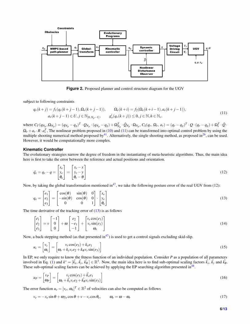
In this Section, first, an NMPC-based path planner is to generate reference trajectory to reach the current destination pose,additionally satisfying the collision avoidance constrain. Second, an EP-based gain tuning method is designed to generateKC-based velocity commands. Third, a dynamic control is designed with the NDO to mitigate the effects of disturbances andtreat the skid-slip effect. Finally, the stability analysis of the proposed controller is discussed. Figure 2 illustrates the overallclose-loop structure of the proposed technique.
NMPC-based path planner
we will consider NMPC-based path planner to generate a reference trajectory for the UGV from a starting pose q(0). Inparticular, the the presences of static and dynamic objects are considered in the environment of the UGV. For the referenceposture of the UGV, we consider that the platform operates free of skid-slip, which corresponds to the assumption of purerolling. Thus, by using the pure rolling, the kinematics and dynamics of the UGV can be expressed as46
qr = S(qr) ·Ωr, Ωr = ar (6)
where ar = [v , ω]T and Ωr = [vr, ωr]T . Until now, we have taken we have modelled the platform by a continuous time model.
as a continuous-time system. However, it is essential for a computer to generate discrete signals. Therefore, by using Euler’sapproximation with Ts, we can approximate our nonlinear continuous-time system by a discrete-time one, as follows
The discrete indexing k ∈ Λ, while Λ is a set of positive natural numbers. In terms of collision avoidance, the UGV must movewith some restrictions. Therefore, we have set constraints on the platform’s physical position as follows:
gio(qr(k)) =
√
(x(k)− xio(k))
2 +(y(k)− yio(k))
2 − (rc + rio) (8)
where obstacles are i = 1,2, . . . , I; I represent number of currently known obstacles. Additionally, constraints on the velocitiesand accelerations are considered, as follows:
vrmin≤ vr(k)≤ vrmax , ωrmin
≤ ωr(k)≤ ωrmax , vrmin≤ vr(k)≤ vrmax , ωrmin
≤ ωr(k)≤ ωrmax . (9)
Now, we can compute the cost-function for our NMPC-based path planner as follows:
argminar
J(ar(k+ j)) =CT (qNp ,ΩNp)+Np−1
∑j=0
CS(qr(k+ j),Ωr(k+ j),ar(k+ j)) (10)
5/13
Figure 2. Proposed planner and control structure diagram for the UGV
Ωr +ar ·R ·aTr , The nonlinear problem proposed in (10) and (11) can be transformed into optimal control problem by using the
multiple shooting numerical method proposed by41. Alternatively, the single shooting method, as proposed in26, can be used.However, it would be computationally more complex.
Kinematic ControllerThe evolutionary strategies narrow the degree of freedom in the instantiating of meta-heuristic algorithms. Thus, the main ideahere is first to take the error between the reference and actual positions and orientation.
qe = qr −q =
xe
ye
θe
=
xr − x
yr − y
θr −θ
(12)
Now, by taking the global transformation mentioned in47, we take the following posture error of the real UGV from (12):
qe =
e1
e2
e3
=
cos(θ) sin(θ) 0−sin(θ) cos(θ) 0
0 0 1
·
xe
ye
θe
(13)
The time derivative of the tracking error of (13) is as follows
e1
e2
e3
= v
−100
+ω
e2
−e1
−1
+
vr cos(e3)vr sin(e3)
ωr
(14)
Now, a back-stepping method (as that presented in47) is used to get a control signals excluding skid-slip.
uc =
[
vc
ωc
]
=
[
vr cos(e3)+ kxe1
ωr + kyvre2 + kθ vr sin(e3)
]
(15)
In EP, we only require to know the fitness function of an individual population. Consider P as a population of all parametersinvolved in Eq. (1) and k∗ = [kx, ky, kθ ] ∈ R
3. Now, the main idea here is to find sub-optimal scaling factors kx, ky and kθ .These sub-optimal scaling factors can be achieved by applying the EP searching algorithm presented in48.
The dynamics in Eq. (2) can be transferred into the following
M · uP +F = B · τ (18)
with
M = T T MT, B = T T B, T =
[
(xe sinθ − ye cosθ) 11 0
]
,Π = [vr cosθe +ωr(xe sinθ − ye cosθ), ωr]T .
F = T T [MT (ue +Π)+MT Π−Mη +C1(Ω−η)]+T T [C2ρ +C3ρ]+ B · τd ,
The parameter M is unknown. However, the nominal M0 is known, and taking the velocity tracking error ζ = ue −uP, we have
ζ = M0−1
B · τ +H · B · τ − M−1·F − uP (19)
where H = M−1 − M0−1. In addition, we can take ∆τ = (τ(k+1)− τ(k)) to handle the saturation constraints. This will also
gives an intuition that uP is related to unknown skid-slip. Therefore the above expression becomes as follows
ζ = M0−1
Bτ +∆τ +H · B · τ − M−1F − uP − (M0−1
B− I)∆τ (20)
To accomplish the NDO, we first need to lumped the estimated disturbances as follows
ˆζ = L(q) · (ζ − ζ ) (21)
where L(q) is the observer gain. Now, we can define the auxiliary variable D to obtain an improved disturbance observer designas follows:
ˆD = L(q) · (M0−1
B · τ +H · B · τ − M−1·F − uP)−L(q) · ˆ
ζ , ζ = D+ p(uP) (22)
where the function p(up) is selected from49.
p(uP) = K ·uP, p(uP) = K (23)
where K is the constant matrix. Now, by taking the time derivative of (22)
ˆζ = D+ p(uP) · uP (24)
By combining the expressions Eq. (21) and Eq. (22)
ˆζ − ˆD = L(q) · MuP, L(q) · M = p(uP) (25)
Thus, we select the observer gain matrix as L(q) = K · M−1. Now, using Eq. (19) and Eq. (22) the expression can be re-writtenas follows:
ζ = M−10 · B · τ +∆τ + D (26)
For the system proposed in (26) the applied torque can be achieved as follows:
τ = M0−1
· B · [−α ·ζ +β ·Kc −β 2ζ
2− D] (27)
The stability analysis of the observer is performed as per26. Therefore, we will discuss the closed loop stability analysis of thecontroller scheme in the following subsection.
Results and Discussions
In this section, we discuss the simulation-based experiments performed in MATLAB. The physical parameters of UGVare set as follows: b = 0.67 m, r = 0.30 m, d = 0.6 m, mc = 50 kg, mw = 2kg, J = 15 kgm2.The skid-slip are considered as[η1, η2,µ] = 0.02 · [sin(0.3t), 1, 1]. The external torque-based disturbance td = [0.01cos(0.5t)0.01sin(0.5t)]T .
For NMPC gain tuning, we have selected the weighting matrices Q = diag[5, 10, 0.01], Q = diag[10, 10, 10], and R =diag[0.05, 0.05]. The prediction horizon of Np = 20 for the simulations related to path-tracking, and Np = 22, the simulationsrelated to tracking a circle. Additionally, the sample time of Ts = 0.01 s is selected. The input torque is saturated and assumedto be τmin = −100 Nm and τmax = 100 Nm. Finally, voltages on the right and left motors are Vrmin
= −12V , Vrmax = 12V ,Vlmin
=−12V and Vlmax= 12V , respectively.
7/13
[a]200 400 600 800 1000 1200
x[m]
100
200
300
400
500
600
y[m
]
0
50
100
150
200
250
300
Goal
Start
Trajectory
MO
UGV
SO
Prediction
[b]739 740 741 742 743 744 745 746
x[m]
198.5
199
199.5
200
200.5
201
y[m
]
[c]
0 100 200 300 400 500 600
Time[s]
-0.5
0
0.5
1
1.5
Lo
ng
itu
din
al
ve
loc
ity
[m/s
]
0 100 200 300 400 500 600
Time[s]
-40
-20
0
20
40
Ya
w R
ate
[d
eg
/s]
[d]x
ey
e e
-0.05
-0.04
-0.03
-0.02
-0.01
0
0.01
0.02
0.03
Median
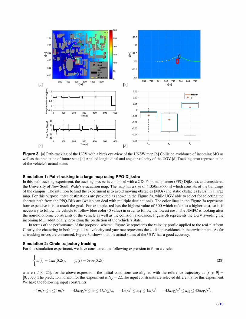
Figure 3. [a] Path-tracking of the UGV with a birds eye-view of the UNSW map [b] Collision avoidance of incoming MO aswell as the prediction of future state [c] Applied longitudinal and angular velocity of the UGV [d] Tracking error representationof the vehicle’s actual states
Simulation 1: Path-tracking in a large map using PPQ-DijkstraIn this path-tracking experiment, the tracking process is combined with a 2 DoF optimal planner (PPQ-Dijkstra), and consideredthe University of New South Wale’s evacuation map. The map has a size of (1350mx600m) which consists of the buildingsof the campus. The intuition behind the experiment is to avoid moving obstacles (MOs) and static obstacles (SOs) in a largemap. For this purpose, three destinations are provided as shown in the Figure 3a, while UGV able to select for selecting theshortest path from the PPQ-Dijkstra (which can deal with multiple destinations). The color lines in the Figure 3a representshow expensive it is to reach the goal. For example, red has the highest value of 300 which refers to a higher cost, so it isnecessary to follow the vehicle to follow blue color (0 value) in order to follow the lowest cost. The NMPC is looking afterthe non-holonomic constraints of the vehicle as well as the collision avoidance. Figure 3b represents the UGV avoiding theincoming MO, additionally, providing the prediction of the vehicle’s state.
In terms of the performance of the proposed scheme, Figure 3c represents the velocity profile applied to the real-platform.Clearly, the chattering in both longitudinal velocity and yaw rate represents the collision avoidance in the environment. As faras tracking errors are concerned, Figure 3d shows that the actual states of the UGV has a good accuracy.
Simulation 2: Circle trajectory tracking
For this simulation experiment, we have considered the following expression to form a circle:
xr(t) = 5sin(0.2t), yr(t) = 5cos(0.2t) (28)
where t ∈ [0, 25], for the above expression, the initial conditions are aligned with the reference trajectory as [x, y, θ ] =[0, ,0 ,0].The prediction horizon for this experiment is Np = 22.The input constraints are selected differently for this experiment.We have the following input constraints:
Figure 4. [a] Avoided first SO and MO by predicting them. [b] Speeds up to safely overtake the incoming vehicle. [c]Catching up the RT [d] Avoiding another SO and predicting incoming MO to slow down. [e] Approaching to the goal location.[f] Safely reached to the goal.
We have considered four SOs and three MOs as shown in the Figure 4. The SOs are located at (x1, y1) = (2, 1),(x2, y2) = (0, 5.5), (x3, y3) = (−3, 1), and (x4, y4) = (−2, 3). All the SOs are having a radius of 0.5m. For MOs, the startinglocations are (x5, y5,θ) = (−8, 10, pi/4), (x6, y6,θ) = (3, 0, pi/2), and (x7, y7) = (4, 2, −pi), while these MOs are subjectto linear obstacles with linear velocities of 0.5 m/s, 0.4 m/s, and 0.6 m/s, respectively. The intention for this simulation is toavoid collisions and follow the reference trajectory. For first collision avoidance, the UGV predicts SO and MO to divert fromthe reference trajectory as shown in the Figure 4a. Since, the longitudinal velocity of the vehicle is 1 m/s, it increases speed toavoid the MO safely as shown in the Figure 4b. In particular, this is an example of a vehicle over taking another vehicle inthe environment. The UGV tracks back on the proposed nominal trajectory, as shown in the Figure 4c, in which the achievedplatform’s trajectory does converge to the nominal trajectory, after a short transient during the collision avoidance event. Soonafter synchronizing with the nominal trajectory, the platforms detects the presence of an unexpected SO, which requires anothercollision avoidance manoeuvre, as shown in Figure 4d. In Figure 4e the platform properly continues the trajectory trackingprocess, for finally dealing with a second incoming DO and an additional SO, both requiring an avoidance treatment, which issuccessfully performed, for finally completing the required trajectory as shown in Figure 4f.
In terms of meeting the input constraints imposed by the NMPC, Figure 5 illustrates the applied velocities and accelerationsto the UGV. The reference velocity is considered as 0.7m/s, which the vehicles tries to match. However, since the environmentis filled with obstacles, it can only reach the reference velocity once the obstacles are avoided as shown in the Figure 5a.Additionally, the longitudinal velocity increases in the time instances 10(sec)−15(sec), which indicates avoidance of obstaclessafely and then converging to the reference velocity. For the angular velocity, a similar trend can be observed in the Figure5b. For the rate of change in the longitudinal and angular velocities in Figure 5c and 5d, chattering are visible in the signal.However, it always converges to zero once it meets the reference trajectories. The reason for having chattering are due to the
9/13
[a]0 5 10 15 20 25
Time (seconds)
0.6
0.65
0.7
0.75
0.8
0.85
0.9
0.95
1
v (
m/s
)
Reference velocity
Actual velocity
[b]0 5 10 15 20 25
Time (seconds)
-20
-10
0
10
20
30
40
50
(d
eg
/s)
[c]0 5 10 15 20 25
Time(s)
-0.6
-0.4
-0.2
0
0.2
0.4
0.6
a1(m
/s2)
[d]0 5 10 15 20 25
Time(s)
-30
-20
-10
0
10
20
30
40
50
a2(d
eg
/s2)
Figure 5. [a] Longitudinal velocity applied to the UGV in the simulation experiment 3. [b] Angular velocity applied to theUGV in the simulation experiment 3. [c] Rate of change in the longitudinal velocity applied to the UGV in the simulationexperiment 3. [d] Rate of change in the angular velocity applied to the UGV in the in the simulation experiment 3.
[a]Ox
eOy
eO
ex
ey
e e
-0.4
-0.2
0
0.2
0.4
0.6
0.8
Median
[b]0 5 10 15 20 25
Time(s)
-6
-4
-2
0
2
4
6
8
Vo
lta
ge
(V)
Voltage 1
Voltage 2
Figure 6. [a] Box plot to distinguish the actual state tracking errors; where pose (x,y) are in cm and heading is in rad.Additionally, Oxe, Oye and Oθe represents obstacles case. [b] Applied voltages to the UGV in the simulation experiment 3.
Table 1. NMPC average PT/I for single and multi-core CPUs
Np Single Core this paper Single Core26 Multi-Core this paper Multi-Core26
15 1.2 ms 10.3 ms 1 ms 10 ms50 3.32 ms 21.47 ms 3 ms 21 ms
100 10.6 ms 38.61 ms 10 ms 38 ms150 17.8 ms 51.82 ms 17 ms 51 ms
continuous occurrence of multiple obstacles, which diverts the UGV from it’s nominal trajectory.
In terms of trajectory tracking error, we have computed a case with no obstacles and compared it with the one, which wehave simulated in this experiment as shown in the Figure 6a. The mean error for both situations are respectable. However, it isappreciable that without obstacles the tracking error is very small, while the error with obstacles are still having reasonablevalues. Additionally, for control action applied to the UGV, the applied voltages are converging to a steady-state as shown inthe Figure 6b, which proves that motor would work adequately despite these challenging conditions of obstacles and skid-slip.
10/13
Table 2. Comparison of Euclidean distance accuracy among MS and SS numerical methods
To validate the robustness of the proposed method, we have evaluated our method with26. The comparison is performed as perthe error accuracy, capability of the NMPC to run on a single core and multiple cores CPU, and average processing time ofthe NMPC to compute a single optimization iteration. As mentioned earlier in the paper, our numerical method is based onmultiple shooting problem, which is tested in different prediction horizon of time.
The ability to perform any optimization method on an on-board processor must be feasible. For instance, a single-core CPUwith limited resources must be able to solve the optimization problem effectively. For this comparison, Table 1 discusses theproposed method utilizes the average processing time per iteration (PT/I) for this paper (using MS) and compared with SS. Interms of computing NMPC on single or multi-core CPUs, the average PT/I in this paper is relatively better than SS method. Inaddition, even if we increase the prediction horizon to a larger number Np = 150, the PT/I always feasible to run this on theCPU with limited resources. This also enables to perform a real experiment with an on board processor with limited processingcapabilities.
In contrast to26, a remarkable finding is that accuracy in the MS method is optimal for a small and a large predictionhorizon. Although, an increase in the prediction horizons may cause a slower processing but a lower error as shown in thetable 2. However, the issue with increasing a too large prediction horizon isn’t feasible for some cases. For instance, in26, aprediction horizon of Np = 100 was used to run the path planner, which has an accuracy of 2cm. However, this can lead to alarger processing time. Thus, based on these findings, the proposed method is reasonable for real-time applications.
Conclusions
In this paper, we propose a tracking control and planner for a UGV in the presence of a skid-slip and dynamic and staticobjects. The proposed technique consists of a fast NMPC-based path-planner, novel evolutionary programming-based kinematiccontroller, a dynamic controller with a nonlinear disturbance observer, and a voltage driving circuit. We have performedsimulation experiments by considering actual physical parameters to drive the vehicle safely to the goal location. First, a largemap of UNSW is used, which is fed to PPQ-Dijkstra algorithm, and NMPC is combined with the map to avoid collisions andnon-holonomic constraints. Finally, a test in which the UGV must follow a sizeable circular trajectory under the presence ofstatic and moving objects is performed. The results obtained from these experiments validate that the proposed method cansafely drive the vehicle to the goal location. To validate the performance of our proposed technique, we have performed thenumerical multiple-shooting method, being restricted to use only one core and running in multiple cores. Compared to theexisting literature, the proposed technique has improved the processing capability of the NMPC to run in a CPU with limitedresources and improves the error accuracy.
References
1. Choset, H. M. et al. Principles of robot motion: theory, algorithms, and implementation (MIT press, 2005).
2. Kanayama, Y., Kimura, Y., Miyazaki, F. & Noguchi, T. A stable tracking control method for a non-holonomic mobilerobot. In IROS, 1236–1241 (1991).
3. Sun, H. et al. Application of the udwadia–kalaba approach to tracking control of mobile robots. Nonlinear Dyn. 83,389–400 (2016).
4. Biswas, J. & Veloso, M. Depth camera based indoor mobile robot localization and navigation. In 2012 IEEE International
Conference on Robotics and Automation, 1697–1702 (IEEE, 2012).
5. Thrun, S. Learning metric-topological maps for indoor mobile robot navigation. Artif. Intell. 99, 21–71 (1998).
6. Bailey, T. Mobile robot localisation and mapping in extensive outdoor environments (Citeseer, 2002).
7. Hagras, H., Callaghan, V. & Collry, M. Outdoor mobile robot learning and adaptation. IEEE Robotics & Autom. Mag. 8,53–69 (2001).
11/13
8. Dong, W. & Kuhnert, K.-D. Robust adaptive control of nonholonomic mobile robot with parameter and nonparameteruncertainties. IEEE Transactions on Robotics 21, 261–266 (2005).
9. Low, C. B. & Wang, D. Gps-based tracking control for a car-like wheeled mobile robot with skidding and slipping.IEEE/ASME transactions on mechatronics 13, 480–484 (2008).
10. Odry, Á., Fuller, R., Rudas, I. J. & Odry, P. Kalman filter for mobile-robot attitude estimation: Novel optimized andadaptive solutions. Mech. systems signal processing 110, 569–589 (2018).
11. ZUO, S.-l. Mechanical fault diagnosis and repair of the mobile robot based on" four diagnosis methods". DEStech
Transactions on Comput. Sci. Eng. (2019).
12. He, W., Li, Z. & Chen, C. P. A survey of human-centered intelligent robots: issues and challenges. IEEE/CAA J. Autom.
Sinica 4, 602–609 (2017).
13. Niloy, A. et al. Critical design and control issues of indoor autonomous mobile robots: A review. IEEE Access (2021).
14. Mohanan, M. & Salgoankar, A. A survey of robotic motion planning in dynamic environments. Robotics Auton. Syst. 100,171–185 (2018).
15. Rubio, F., Valero, F. & Llopis-Albert, C. A review of mobile robots: Concepts, methods, theoretical framework, andapplications. Int. J. Adv. Robotic Syst. 16, 1729881419839596 (2019).
16. Qu, Z., Wang, J., Plaisted, C. E. & Hull, R. A. Global-stabilizing near-optimal control design for nonholonomic chainedsystems. IEEE Transactions on Autom. Control. 51, 1440–1456 (2006).
17. Morin, P. & Samson, C. Control of nonholonomic mobile robots based on the transverse function approach. IEEE
Transactions on robotics 25, 1058–1073 (2009).
18. Li, Z. et al. Trajectory-tracking control of mobile robot systems incorporating neural-dynamic optimized model predictiveapproach. IEEE Transactions on Syst. Man, Cybern. Syst. 46, 740–749 (2015).
19. Shi, D., Zhang, J., Sun, Z., Shen, G. & Xia, Y. Composite trajectory tracking control for robot manipulator with activedisturbance rejection. Control. Eng. Pract. 106, 104670 (2021).
20. Zhang, X., Wang, R., Fang, Y., Li, B. & Ma, B. Acceleration-level pseudo-dynamic visual servoing of mobile robots withbackstepping and dynamic surface control. IEEE Transactions on Syst. Man, Cybern. Syst. 49, 2071–2081 (2017).
21. Xie, Y. et al. Coupled fractional-order sliding mode control and obstacle avoidance of a four-wheeled steerable mobilerobot. ISA transactions 108, 282–294 (2021).
22. Saenz, A. et al. Velocity control of an omnidirectional wheeled mobile robot using computed voltage control with visualfeedback: Experimental results. Int. J. Control. Autom. Syst. 19, 1089–1102 (2021).
23. Fateh, M. M. & Arab, A. Robust control of a wheeled mobile robot by voltage control strategy. Nonlinear Dyn. 79,335–348 (2015).
24. Sathya, A. et al. Embedded nonlinear model predictive control for obstacle avoidance using panoc. In 2018 European
control conference (ECC), 1523–1528 (IEEE, 2018).
25. Hu, Y. et al. Nonlinear model predictive control for mobile medical robot using neural optimization. IEEE Transactions on
Ind. Electron. (2020).
26. Lu, Q. et al. Targeting posture control with dynamic obstacle avoidance of constrained uncertain wheeled mobile robotsincluding unknown skidding and slipping. IEEE Transactions on Syst. Man, Cybern. Syst. (2020).
27. Patle, B., Pandey, A., Parhi, D., Jagadeesh, A. et al. A review: On path planning strategies for navigation of mobile robot.Def. Technol. 15, 582–606 (2019).
28. Chang, L., Shan, L., Jiang, C. & Dai, Y. Reinforcement based mobile robot path planning with improved dynamic windowapproach in unknown environment. Auton. Robots 45, 51–76 (2021).
29. Xiao, H. & Chen, C. P. Time-varying nonholonomic robot consensus formation using model predictive based protocol withswitching topology. Inf. Sci. 567, 201–215 (2021).
30. Dao, P. N., Nguyen, H. Q., Nguyen, T. L. & Mai, X. S. Finite horizon robust nonlinear model predictive control forwheeled mobile robots. Math. Probl. Eng. 2021 (2021).
31. Sun, Z., Xia, Y., Dai, L., Liu, K. & Ma, D. Disturbance rejection mpc for tracking of wheeled mobile robot. IEEE/ASME
Transactions On Mechatronics 22, 2576–2587 (2017).
12/13
32. Khan, S., Guivant, J. & Li, X. Design and experimental validation of a robust model predictive control for the optimaltrajectory tracking of a small-scale autonomous bulldozer. Robotics Auton. Syst. 103903 (2021).
33. Khan, S. & Guivant, J. Nonlinear model predictive path-following controller for a small-scale autonomous bulldozer foraccurate placement of materials and debris of masonry in construction contexts. IEEE Access 9, 102069–102080 (2021).
34. Khanpoor, A., Khalaji, A. K. & Moosavian, S. A. A. Modeling and control of an underactuated tractor-trailer wheeledmobile robot. Robotica 35, 2297–2318 (2017).
35. Juang, C.-F., Jeng, T.-L. & Chang, Y.-C. An interpretable fuzzy system learned through online rule generation andmultiobjective aco with a mobile robot control application. IEEE transactions on cybernetics 46, 2706–2718 (2015).
36. Wang, D. & Low, C. B. Modeling skidding and slipping in wheeled mobile robots: control design perspective. In 2006
IEEE/RSJ International Conference on Intelligent Robots and Systems, 1867–1872 (IEEE, 2006).
37. Wei, S., Zefran, M., Uthaichana, K. & DeCarlo, R. A. Hybrid model predictive control for stabilization of wheeled mobilerobots subject to wheel slippage. In Proceedings 2007 IEEE International Conference on Robotics and Automation,2373–2378 (IEEE, 2007).
38. Chen, M. Robust tracking control for self-balancing mobile robots using disturbance observer. IEEE/CAA J. Autom. Sinica
4, 458–465 (2017).
39. Li, L., Wang, T., Xia, Y. & Zhou, N. Trajectory tracking control for wheeled mobile robots based on nonlinear disturbanceobserver with extended kalman filter. J. Frankl. Inst. 357, 8491–8507 (2020).
40. Chen, M., Shi, P. & Lim, C.-C. Robust constrained control for mimo nonlinear systems based on disturbance observer.IEEE Transactions on Autom. Control. 60, 3281–3286 (2015).
41. Andersson, J. A., Gillis, J., Horn, G., Rawlings, J. B. & Diehl, M. Casadi: a software framework for nonlinear optimizationand optimal control. Math. Program. Comput. 11, 1–36 (2019).
42. Jin, X., Yu, J., Qin, J., Zheng, W. X. & Chi, J. Adaptive perturbation rejection control and driving voltage circuit designs ofwheeled mobile robots. J. Frankl. Inst. 358, 1185–1213 (2021).
43. Robledo, A., Guivant, J. & Cossell, S. Pseudo priority queues for real-time performance on dynamic programmingprocesses applied to path planning. In Australasian Conference on Robotics and Automation (2010).
44. Wang, D. & Low, C. B. Modeling and analysis of skidding and slipping in wheeled mobile robots: Control designperspective. IEEE Transactions on Robotics 24, 676–687 (2008).
45. Chen, M. Disturbance attenuation tracking control for wheeled mobile robots with skidding and slipping. IEEE Transactions
on Ind. Electron. 64, 3359–3368 (2016).
46. Fierro, R. & Lewis, F. L. Control of a nonholonomic mobile robot using neural networks. IEEE transactions on neural
networks 9, 589–600 (1998).
47. Slotine, J.-J. E., Li, W. et al. Applied nonlinear control, vol. 199 (Prentice hall Englewood Cliffs, NJ, 1991).
48. Chen, C.-Y., Li, T.-H. S. & Yeh, Y.-C. Ep-based kinematic control and adaptive fuzzy sliding-mode dynamic control forwheeled mobile robots. Inf. Sci. 179, 180–195 (2009).
49. Chen, W.-H., Ballance, D. J., Gawthrop, P. J. & O’Reilly, J. A nonlinear disturbance observer for robotic manipulators.IEEE Transactions on industrial Electron. 47, 932–938 (2000).
Competing interests
The authors declare no competing interests.
Author contributions statement
Subhan Khan prepared Model Predictive Control, Kinematic and Dynamic control, simulation results, figures, and tables. Joseguivant prepared PPQ-Dijkstra algorithm, provided the UNSW Map, and suggested the idea of Simulation 1. All authorsreviewed the manuscript.