One of the primary needs of operational numericalweather prediction ~NWP! centers and an importantaim of the World Climate Research Program is toimprove our understanding of the atmospheric andsurface hydrological cycle @Global Energy and WaterCycle Experiment ~GEWEX! science plan1#. This isa prerequisite for making improvements in NWPmodels. Another requirement of the climate changecommunity is to monitor the concentrations of theatmospheric minor constituents consistently over along period of time.
One step forward in these objectives will be theavailability of high-resolution infrared sounder dataon operational meteorological polar orbiters, whichwill provide temperature and constituent profiles at ahigher accuracy and with more vertical resolutionthan the existing filter wheel radiometers. The In-frared Atmospheric Sounding Interferometer ~IASI!has been designed as an advanced infrared sounderon the next generation of operational meteorologicalpolar orbiters. In combination with the Advanced
The authors are with the European Center for Medium-RangeWeather Forecasts, Shinfield Park, Reading RG2 9AX, UK. Thee-mail address for M. Matricardi is [email protected].
Received 9 December 1998; revised manuscript received 6 July1999.
Microwave Sounding Unit, the Microwave HumiditySounder, and the Advanced Very High ResolutionRadiometer, this is the core payload of the EuropeanOrganisation for Exploitation of MeteorologicalSatellites ~EUMETSAT! Meteorological OperationalSatellite ~METOP-1! and will contribute to the pri-mary mission objective of METOP-1 that is the mea-surement of meteorological parameters for NWP andclimate models.
The IASI instrument is a Fourier-transform spec-trometer. The design of the interferometer is basedon a classical Michelson instrument with a 22- to
2-cm optical path difference range. The IASI has aonstant spectral sampling interval of 0.25 cm21, andt will cover the spectral range from the CH4 absorp-
tion band at 3.62 mm ~2760 cm21! to the CO2 absorp-tion band at 15.5 mm ~645 cm21! with an unapodizedspectral resolution between 0.35 and 0.5 cm21. TheASI measures from a polar orbit the spectrum ofnfrared radiation emitted by the Earth’s atmospherend surface with the objective of providing improvedropospheric soundings of temperature, moisture,nd some minor constituents, and documenting theadiative spectral properties of surfaces and clouds.he IASI spectral range is divided into three bandsanging from 645 to 1210 cm21 ~band one!, from 1210
to 2000 cm21 ~band two!, and from 2000 to 2760 cm21
~band three!. Band one will be used primarily fortemperature and ozone sounding, band two for watervapor sounding and for the retrieval of N2O and CH4column amounts, whereas band three will be used for
0 September 1999 y Vol. 38, No. 27 y APPLIED OPTICS 5679
asfisrfthl
pf
4
acTfg
dttid~afwcwpa
w
ttuffl
5
temperature sounding and for the retrieval of N2Ond CO column amounts. In particular the IASIystem is expected to provide information on the pro-les of temperature in the free troposphere and lowertratosphere to an accuracy of 1 K and a verticalesolution of 1 km. Profiles of water vapor in theree troposphere and lower stratosphere are expectedo be inferred with an accuracy of 10% in relativeumidity and a vertical resolution of 1–2 km in the
ow troposphere.Given the potential benefits of the IASI for NWP,
reparations are being made at the European Centreor Medium-Range Weather Forecasts ~ECMWF! for
exploitation of the IASI datasets. In recent yearsthe ECMWF has moved from the use of retrievedtemperature and humidity profiles from the Televi-sion InfraRed Observation Satellite ~TIROS-N! Op-erational Vertical Sounder ~TOVS!2 to assimilatingthe radiances directly into the model by use of avariational analysis scheme, for example, 1D-Var de-scribed by Eyre et al.3 for a single profile retrieval orD-Var described by Rabier et al.4 for a global NWP
analysis. A prerequisite for exploiting the IASI ra-diance data in the NWP model by use of the varia-tional analysis scheme is the development of a fastradiative transfer ~RT! model to predict IASI radi-ances accurately given first-guess-model fields oftemperature, water vapor, ozone, surface emissivity,and perhaps cloud at a later time. This fast RTmodel has to simulate part of or all the IASI radiancespectrum for each observation point to give the modelequivalent of the observation with which the mea-surement is compared. The fast RT model is alsorequired for prelaunch studies to predict the range ofradiances that the instrument will measure. Itmust be fast enough to cope with the processing ofobservations in near real time and with the severalthousands of transmittance calculations required tosimulate radiances from a full range of atmosphericconditions.
The ECMWF uses the clear radiances operation-ally from the TOVS. The model used to process datafrom the High-Resolution Infrared RadiationSounder ~HIRS! and the Advanced MicrowaveSounding Unit carried on the National Oceanic andAtmospheric Administration polar orbiting satelliteis the radiative transfer for Tiros Operational Verti-cal Sounder ~RTTOV!.5
The fast RT model developed at the ECMWF forexploitation of IASI radiances is based on the ap-proach followed by RTTOVS. It contains a fastmodel of the transmittances of the atmospheric gasesthat is generated from accurate line-by-line transmit-tances for a set of diverse atmospheric profiles overthe IASI wave-number range. The monochromatictransmittances are convolved with the appropriateIASI instrument spectral response function ~ISRF!nd are used to compute channel-specific regressionoefficients by use of a selected set of predictors.hese regression coefficients can then be used by the
ast transmittance model to compute transmittancesiven any other input profile. This parameteriza-
680 APPLIED OPTICS y Vol. 38, No. 27 y 20 September 1999
tion of the transmittances makes the model compu-tationally efficient and in principle should not addsignificantly to the errors generated by uncertaintiesin the spectroscopic data used by the line-by-linemodel. The RTTOVS approach is used operation-ally at several NWP centers. A different approachknown as the optical path transmittance method wasdeveloped recently by McMillin et al.6,7 and imple-mented at the National Center for EnvironmentalPrediction ~NCEP!.
Here we deal with the methods that were applied toevelop the RTIASI, the ECMWF fast RT model forhe IASI. The methods involve the formulation ofhe RT model ~Section 2!, the selection of a new train-ng set of atmospheric profiles ~Section 3!, the pro-uction of a line-by-line transmittance databaseSection 4!, and the selection of optimal predictorsnd the production of regression coefficients for theast transmittance scheme ~Section 5!. In Section 6e describe the results of a comparison of radiances
omputed with the line-by-line transmittances andith the fast RT model for a dependent and an inde-endent set of profiles, respectively. Conclusionsre given in Section 7.
2. Formulation of the Radiative Transfer Model
The current formulation of the RTIASI assumes that,for a plane-parallel atmosphere in local thermody-namic equilibrium with no scattering, the upwellingradiance at the top of the atmosphere can be writtenas8
R~n, u! 5 ~1 2 N!Rclr~n, u! 1 NRcld~n, u!, (1)
here Rclr~n, u! and Rcld~n, u! are the clear-columnand overcast radiances at wave number n and zenithangle u and N is the fractional cloud cover assumedhere to be in a single layer with unit cloud top emis-sivity. If we assume specular reflection at theEarth’s surface, the monochromatic clear-column ra-diance can be written as9
Rclr~n, u! 5 ts~n, u!es~n, u!B~n, Ts! 1 *ts
1
B~n, T!dt
1 @1 2 es~n, u!#ts2~n, u!*
ts
1
~B~n, T!yt2!dt,
(2)
where B~n, T! is Planck’s function for scene temper-ature T, t is the atmospheric level-to-space transmit-tance, and es~n, u! is the surface emissivity; here thesubscript s refers to the surface. Note that the firstand third terms on the right-hand side of Eq. ~2! arehe radiance from the surface and the second term ishe radiance emitted by the atmosphere. In partic-lar, the third term is the thermal radiance reflectedrom the surface. It is important to include the re-ected thermal radiance in Eq. ~2! because a proper
treatment of this term helps separate surface tem-perature from surface emissivity.
cld
t
wcnT
w
s
cs
av
it
R ~n, u! is defined as
Rcld~n, u! 5 tcld~n, u!B~n, Tcld! 1 *tcld
1
B~n, T!dt, (3)
where tcld~n, u! is the cloud top-to-space transmit-ance, and Tcld is the cloud top temperature. To rep-
resent the outgoing radiance as viewed by the IASI,the spectrum of monochromatic radiance given by Eq.~1! must be convolved with the appropriate ISRF.One can usually write
R~n*, u! 5 *2`
1`
R~n, u! f ~n* 2 n!dn, (4)
here f ~n* 2 n! is the normalized ISRF and the cir-umflex over the symbol denotes convolution. Here
˜* is the central wave number of the IASI channel.he monochromatic radiance R~n, u! can be computed
accurately by a line-by-line model, but the whole pro-cess of calculating and convolving the monochromaticradiance is too time-consuming to be performed inreal time. Here we follow the approach of comput-ing approximate convolved radiances assuming thatEq. ~1! can be applied to the spectrally averaged ra-diance and the spectrally averaged transmittance.The radiance calculation is performed assuming thatthe atmosphere is subdivided into a number of homo-geneous layers of fixed pressure. We can rewrite Eq.~1! in discrete layer notation for L atmospheric layers~the atmospheric layers are numbered from space,layer 1, to the first layer above the surface, layer L!and for a single viewing angle to simplify the nota-tion:
Rn*clr 5 ts,n*es,n*Bn*~Ts! 1 S(
j51
L
Rj,n*uD 1 ~1 2 es,n*!
3 F(j51
L
Rj,n*u~ts,n*
2ytj,n* tj21,n*!G 1 Rn*9 (5)
here tj,n* is the convolved transmittance from agiven pressure level pj to space and Rj,n*
u is defined as
Rj,n*u 5 Bn*~Tj!~tj21,n* 2 tj,n*!. (6)
Rn*9 is a small atmospheric contribution from thesurface to the first layer above the surface L. Notethat in deriving Eq. ~5! we implicitly assume that thetotal transmittance of an atmospheric path is theproduct of the transmittances of the constituent sub-paths. Although this is true for monochromatic ra-diation, it can be considered a good approximationwhen the transmittance varies relatively slowly withwave number ~note that the IASI ISRF is narrow andis essentially symmetric about its centroid!. Thecene temperature Tj is defined here as the layer
mean temperature that was obtained by use of theCurtis–Godson air density weighted mean value as-suming that the temperature varies linearly betweenthe layer boundaries. The calculation of the sea sur-face emissivity es,n*~u! can be performed by use of themodel of Masuda et al.10 The refractive index of
20
pure water based on Hale and Querry11 is adjusted~Friedman12! to the seawater value and then inter-polated to the wave number n* to be given as an inputwith surface wind speed and the zenith angle u toompute the rough sea surface emissivity. Figure 1hows the range spanned by es,n*~u! for a number of
different situations assuming an average wind speedof 7 m s21. Over land the emissivity is set to 0.97.The top of atmosphere overcast cloudy radiance indiscrete notation is defined as
Rn*cld 5 tcld,n*Bn*~Tcld! 1 Rn*0 1 (
j51
Lcl
Rj,n*u, (7)
where Lcl is the layer above the cloud top and there isan interpolation of the radiance from the level belowthe cloud top and the level above the cloud top de-noted by Rn*0 to provide the additional radiance fromthe last full layer to the cloud top. Finally one canmake an empirical correction to the transmittance byraising the computed transmittance to the power g,where g is determined empirically. In this paper g isset equal to 1. We tested the validity of Eq. ~5! bycomparing the convolved monochromatic radiances~at a resolution of 0.001 cm21! with the radiancescomputed from the convolved transmittances.These exact and approximate convolved radianceswere computed for a set of 34 atmospheric profiles~see below! and compared. The differences weretypically less than 0.12 K. Inasmuch as the errorintroduced by this polychromatic approximation isless than the radiometric noise it was considered to beadequate for our purposes.
For a given input atmospheric profile ~tempera-ture, water vapor, and ozone volume mixing ratio!and surface variables ~emissivity, pressure, temper-ture, skin temperature!, the computation of the con-olved level-to-space transmittance tj,n* or convolved
level-to-space optical depth dj,n* ~tj,n* 5 exp 2 @dj,n*#!s performed by the fast transmittance model and ishe essence of the RTIASI. Here we assume that the
Fig. 1. Computed sea surface emissivity for the IASI channels.The wind speed is set to a reference value of 7 m s21.
September 1999 y Vol. 38, No. 27 y APPLIED OPTICS 5681
dtbfinsfrtss
Table 1. Minimum and Maximum Values of the Temperature, Water Vapor, and Ozone Values Used in the Regression at Each Point of the Pressure
5
RT equation is integrated on the same levels as thetransmittance computation although in principle thisis not necessary. The atmosphere is divided into 42layers whose boundaries are the fixed pressure levelslisted in Table 1. As some IASI channels show ab-sorption features even for very low values of pressure,transmittances are computed also for an additionallayer between 0.1 and 0.005 hPa. The number oflevels is a compromise between the computing re-sources and the need to keep the RT errors below theinstrument noise. To quantify the errors that areintroduced by limiting the number of layers to 43, wecompared the spectra obtained by dividing the atmo-
682 APPLIED OPTICS y Vol. 38, No. 27 y 20 September 1999
sphere into 43 and 98 layers for two different atmo-spheric profiles ~tropical and high latitude!. The
ifference between the convolved spectra was foundo be less than 0.05 K in band 1, less than 0.08 K inand 2, and less than 0.15 K in band 3, all thesegures being significantly lower than the instrumentoise. Inasmuch as the troposphere and the lowertratosphere represent the most important regionsor the IASI, the thicknesses of the layers in thoseegions were selected to be less than or at least equalo the nominal IASI 1-km vertical resolution. Ashown in Table 1, the thickness of the layers variesmoothly with pressure to avoid significant changes
in layer optical depths and to ease interpolation ~ei-her within the line-by-line computations or if the RTquation is integrated on another set of levels!; careust also be taken to select an adequate number of
evels around the tropopause and the boundary lay-rs.The fast transmittance stage of the RTIASI is
ased on algorithms that have been developed overhe years for a number of different satellitenstruments.8,13–19 In the RTIASI fast transmit-ance model the computation of the optical depth forhe layer from pressure level j to space along a path
at angle u involves a polynomial with terms that areunctions of temperature, absorber amount, pressure,nd viewing angle. The convolved optical depth atave number n* from level j to space can be writtens
dj,n* 5 dj21,n* 1 (k51
M
aj,n*,k Xk, j, (8)
where M is the number of predictors and the func-ions Xkj constitute the profile-dependent predictors
of the fast transmittance model. To compute theexpansion coefficients aj,n*,k ~sometimes referred to asfast transmittance coefficients!, one can use a set ofdiverse atmospheric profiles to compute, for each pro-file and for several viewing angles, accurate line-by-line level-to-space transmittances for each leveldefined by the atmospheric pressure layer grid. Theconvolved level-to-space transmittances tj,n* are thenused to compute the aj,n*,k coefficients by linear re-gression of dj,n* 2 dj21,n* @or 2ln~tj,n*ytj21,n*!# versusthe predictor values Xkj calculated from the profilevariables for each profile at each viewing angle.Note that the regression is made on the layer opticaldepths rather than on the level-to-space transmit-tances themselves, as this gives significantly moreaccurate results.17
3. Diverse Profile Dataset
For each gas allowed to vary, the profiles used tocompute the database of line-by-line transmittancesare chosen to represent the range of variations intemperature and absorber amount found in the realatmosphere. Only a few atmospheric gases are al-lowed to vary, the others are held constant and will bereferred to as fixed. Gases are considered as fixed iftheir spatial and temporal concentration variationsdo not contribute significantly to the observed radi-ances. In this paper only H2O and O3 are allowed tovary ~although in localized IASI spectral regionsases such as CO, N2O, and CH4 could also be con-
sidered variable! and fast transmittance coefficientsare generated for H2O, O3, and fixed gases.
As outlined in Section 2, the transmittances com-puted for the diverse profiles become the data pointsin the regression. The water vapor and fixed gasfast transmittance coefficients were derived by use ofa training set of 42 profiles selected from the 1761profile TOVS Initial Guess Retrieval ~TIGR! dataset
20
~for more details see Chedin et al.20!. For the ozoneast transmittance coefficients 33 ozone profiles ~se-ected from a set of 383 profiles from the Nationalnvironmental Satellite Data, and Information Ser-ice supplemented by a few extreme Antarctic pro-les! were used.21 Note that, within the regression
scheme, the global mean of either the 1761 TIGRprofiles and the 383 ozone profiles is included to serveas a reference profile. These profiles were selectedto cover most of the range of observed temperature,water vapor, and ozone behavior. The determina-tion of the number of profiles was arrived at as acompromise between the computational time neededto build up the database and the need to cover therange of profile behavior in the regression.
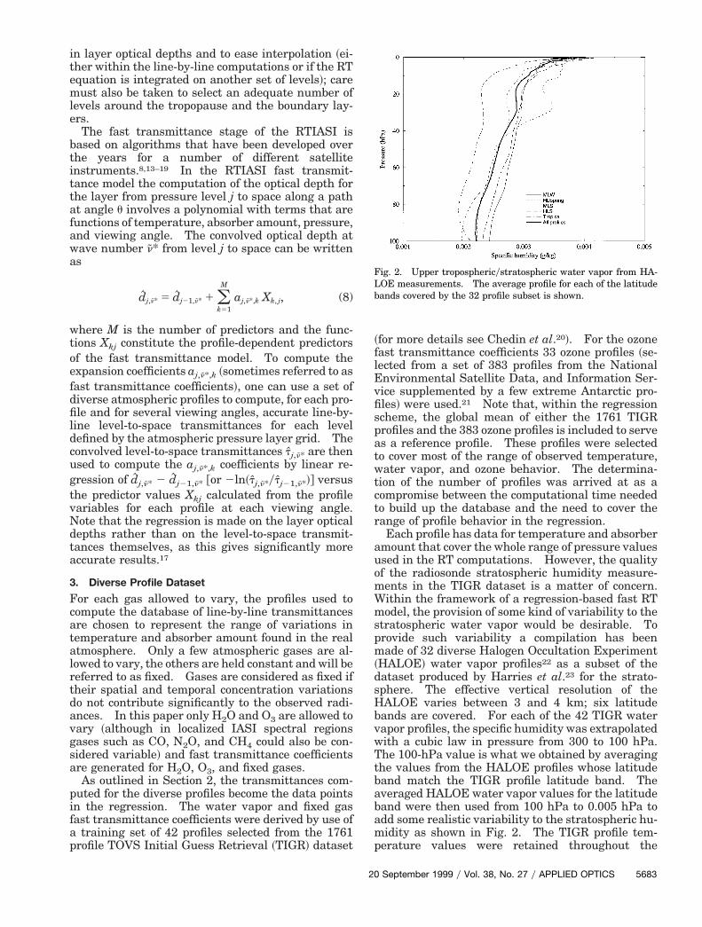
Each profile has data for temperature and absorberamount that cover the whole range of pressure valuesused in the RT computations. However, the qualityof the radiosonde stratospheric humidity measure-ments in the TIGR dataset is a matter of concern.Within the framework of a regression-based fast RTmodel, the provision of some kind of variability to thestratospheric water vapor would be desirable. Toprovide such variability a compilation has beenmade of 32 diverse Halogen Occultation Experiment~HALOE! water vapor profiles22 as a subset of thedataset produced by Harries et al.23 for the strato-sphere. The effective vertical resolution of theHALOE varies between 3 and 4 km; six latitudebands are covered. For each of the 42 TIGR watervapor profiles, the specific humidity was extrapolatedwith a cubic law in pressure from 300 to 100 hPa.The 100-hPa value is what we obtained by averagingthe values from the HALOE profiles whose latitudeband match the TIGR profile latitude band. Theaveraged HALOE water vapor values for the latitudeband were then used from 100 hPa to 0.005 hPa toadd some realistic variability to the stratospheric hu-midity as shown in Fig. 2. The TIGR profile tem-perature values were retained throughout the
Fig. 2. Upper troposphericystratospheric water vapor from HA-LOE measurements. The average profile for each of the latitudebands covered by the 32 profile subset is shown.
September 1999 y Vol. 38, No. 27 y APPLIED OPTICS 5683
ipe
att
5
pressure range, and each profile was checked for su-persaturation and adjusted if necessary. The sameextrapolation and supersaturation check were ap-plied to the water vapor amount values that comewith the ozone profiles.
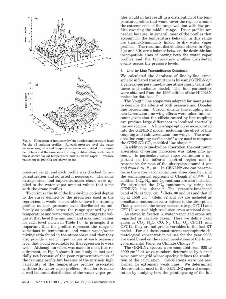
To optimize the fit of the line-by-line optical depthsto the curve defined by the predictors used in theregression, it would be desirable to have the trainingprofiles at each pressure level distributed as uni-formly as possible across the range spanned by thetemperature and water vaporyozone mixing ratio val-ues at that level ~the minimum and maximum valuesfor each level shown in Table 1!. In principle it isimportant that the profiles represent the range ofvariations in temperature and water vaporyozonemixing ratio found in the atmosphere and that theyalso provide a set of input values at each pressurelevel that would be suitable for the regression to workwell. Although an effort was made to meet this re-quirement, as Fig. 3 shows it could only be met par-tially not because of the poor representativeness ofthe training profile but because of the intrinsic highvariability of the temperature profiles associatedwith the dry water vapor profiles. An effort to makea well-balanced distribution of the water vapor pro-
Fig. 3. Histogram of frequency by bin number and pressure levelfor the 43 training profiles. At each pressure level the watervapor mixing ratio and temperature range are divided into a num-ber of bins and the number of training profiles falling within eachbin is shown for ~a! temperature and ~b! water vapor. Pressurevalues up to 100 hPa are shown in ~a!.
684 APPLIED OPTICS y Vol. 38, No. 27 y 20 September 1999
files would in fact result in a distribution of the tem-perature profiles that would cover the regions aroundthe extreme ends of the range well but with few pro-files covering the middle range. Drier profiles areneeded because, in general, most of the profiles thataccount for the temperature behavior in this rangeare thermodynamically linked to dry water vaporprofiles. The resultant distributions shown in Figs.3~a! and 3~b! are a balance between the desirable butncompatible aims of having both the water vaporrofiles and the temperature profiles distributedvenly across the pressure levels.
4. Line-by-Line Transmittance Database
We calculated the database of line-by-line atmo-spheric infrared transmittances by using GENLN2,24
a general-purpose line-by-line atmospheric transmit-tance and radiance model. The line parameterswere obtained from the 1996 edition of the HITRANmolecular database.25
The Voigt26 line shape was adopted for most gasesto describe the effects of both pressure and Dopplerline broadening. Carbon dioxide line-coupling andnon-Lorentzian line-wing effects were taken into ac-count given that the effects caused by line couplingcan produce large differences in localized spectrallynarrow regions. A line-shape option is incorporatedinto the GENLN2 model, including the effect of linecoupling and sub-Lorentzian line wings. The avail-able line-coupling coefficients27 were used to computethe GENLN2 CO2 modified line shape.24
In addition to line-by-line absorption, the continuumabsorption of certain molecules was taken into ac-count. In particular, water vapor continuum is im-portant in the infrared spectral region and isresponsible for most of the absorption around 4 mmnd from 8 to 12 mm. In GENLN2 one can parame-erize the water vapor continuum absorption by usinghe semiempirical approach of Clough et al.28,29 In
addition CO2, N2, and O2 continua are also included.We calculated the CO2 continuum by using theGENLN2 line shape.24 The pressure-broadenedband of N2 at 2350 cm21 ~Refs. 30 and 31! and that ofO2 at 1550 cm21 ~Refs. 32 and 33! are included asbroadband continuum contributions to the absorption.Finally, to model the heavy molecules ~e.g., CFC11 andCFC12! we used high-resolution cross-sectional data.
As stated in Section 3, water vapor and ozone areregarded as variable gases. Here we define fixedgases as CO2, N2O, CO, N2, CH4, O2, CFC11, andCFC12, they are not profile variables in the fast RTmodel. For all these constituents tropospheric cli-matological concentration values for the year 2005are used based on the recommendations of the Inter-governmental Panel on Climate Change.34
The GENLN2 spectra were computed from 600 to3000 cm21 at wave numbers determined by a fixedwave-number grid whose spacing defines the resolu-tion of the calculation. Calculations were not per-formed for extremely weak lines. We determinedthe resolution used in the GENLN2 spectral compu-tation by studying how the point spacing of the full
pIasrsvemar
scs
c
ss
T
olwlocEl1cdTgttut
st
wjdcopgfit
T
resolution spectra affected the convolved radiance.The full resolution spectrum is the spectrum con-volved with the ISRF to generate a simulated spec-trum that can be compared with the observedspectrum. The simplest procedure to generate thefull resolution spectra would be to choose a wave-number grid fine enough that the narrowest line isadequately sampled. This suggests a resolution ashigh as 0.0005 cm21, which for this study was not
ractical in terms of available computing resources.nasmuch as the features of the convolved spectrumre controlled by the spacing of the monochromaticpectrum, we decided to arrive at the definition of fullesolution spectrum by studying how varying thepacing of the wave-number grid changed the con-olved IASI spectra. Two atmospheric profiles atither end of profile extremes were selected, andonochromatic radiance spectra at the top of the
tmosphere were computed at an increasingly higheresolution ~i.e., S1, 0.05 cm21, S2, 0.005 cm21; S3,
0.0025 cm21; S4, 0.001 cm21; S5, 0.0005 cm21!. Thepectra were then convolved and for each profile weompared the IASI radiometric noise figure with thepectra drawn from the differences S1 2 S2, S2 2 S3,
S3 2 S4, and S4 2 S5. The greatest differences werefound to occur in the strong 15-mm CO2 absorptionband for the extreme tropical profile. Over the IASIwave-number range only S4 2 S5 was found to be wellbelow the instrument noise. This means that theextra features we introduced into the convolved spec-tra by increasing the wave-number grid spacing from0.001 to 0.0005 cm21 are so small that the instrumentannot detect them. Hence 0.001 cm21 is a suffi-
cient resolution for the IASI simulations.The diverse profile datasets described in Section 3
have been used to build the database of line-by-linetransmittances required to compute the regressioncoefficients used by the RTIASI fast transmittancemodel. Transmittances were computed from 0.005hPa to each of the 43 standard pressure levels, at0.001-cm21 resolution, for each atmospheric profileand six scan angles, namely, the angles for which thesecant has equally spaced values from 1 to 2.25. Thetransmittance calculations ~and the subsequent con-volution! represented a massive undertaking, thesize of the final database being nearly 500 Gbytes.The convolved line-by-line transmittances were usedto compute three sets of regression coefficients be-cause the fast transmittance model treats separatelythe absorption by the fixed gases, water vapor, andozone.8 For each term we can compute the level-to-pace transmittances by using an algorithm of theame form as in Eq. ~8!, the predictors Xk, j ~defined in
Section 5! depending on the gas. However, in gen-eral, for real, nonmonochromatic channels the convo-lution of the transmittance of all the gases differsfrom the product of the transmittance of the singlegases convolved individually, and the monochromatictransmittance approximation
tn*, jT 5 tn*, j
F tn*, jW tn*, j
O, (9)
20
where tn*, j is the convolved transmittance of all thegases and tn*, j
F, tn*, jW, and tn*, j
O are the transmit-tances of the single gases convolved individually,might not be accurate because, for example, absorp-tion by water vapor is not totally uncorrelated withabsorption by the fixed gases. Even for the narrowIASI channels the convolved transmittance computedwith Eq. ~9! differs significantly from the convolutionf the transmittance of all the gases. The line-by-ine transmittances from the absorbing gas aloneere convolved and compared with the convolved
ine-by-line transmittances from all the gases for thezone reference profile. The difference between theorrect total transmittance and that computed withq. ~9! was found to vary with wave number and with
evel. For example, for some of the channels in the0-mm window region the brightness temperaturesomputed by use of the correct transmittances couldiffer by .0.7 K from those computed with Eq. ~9!.o reduce the errors introduced by separation of theas transmittances after convolution, we calculatedhe monochromatic transmittances and groupedhem into four sets. The water vapor profiles weresed to compute one set of level-to-space transmit-ances for the combined effect of the fixed gases, tn, j
F,and one set for the fixed gases plus water vapor,tn, j
F1WV, whereas the ozone profiles were used tocompute one set of level-to-space transmittances forthe fixed gases plus water vapor t9n, j
~F1WV!, and oneet for the fixed gases plus water vapor and ozone,9n~F1WV1OZ!, where the prime over the symbol de-
notes transmittances from ozone profiles.The monochromatic transmittances were con-
volved and used to compute the fixed gases, watervapor, and ozone layer optical depths defined as
dn*, jF 2 dn*, j21
F 5 2ln~tn*, jFytn*, j21
F!, (10)
dn*, jWV 2 dn*, j21
WV 5 2ln@~tn*, jF1WVytn*, j
F!
3 ~tn*, j21Fytn*, j21
F1W!#, (11)
dn*, jO 2 dn*, j21
O 5 2ln$@tn*, j~F1WV1O!9ytn*, j
~F1WV!9#
3 @tn*, j21~F1W!9ytn*, j21
~F1WV1O!9#%,(12)
here the transmittance from 0.05 hPa to space ~when2 1 5 0! is set equal to 1. Note that the layer opticalepths defined by Eqs. ~11! and ~12! do not involve anyalculation based on absorption of water vapor andzone alone. These layer optical depths are the dataoints used in the regression to generate the fixedases, water vapor, and ozone fast transmittance coef-cients and are used to compute the model transmit-ances tn*, j
Fmodel, tn*, jWVmodel, and tn*, j
Omodel by apolynomial expansion of the same form as in Eq. ~8!.
he total model transmittance can now be written as
tn*, jTmodel 5 tn*, j
Fmodeltn*, jWVmodel tn*, j
Omodel (13)
5. Fast Transmittance Model
The fast model simulates IASI level 1C radiances,which is the radiance product that will be distributed
September 1999 y Vol. 38, No. 27 y APPLIED OPTICS 5685
mto6rt
trgm1
ssTcc
tt
d
fi
Table 2. Definition of Profile Variables Used in Predictors Defined in Table 3a
5
to the NWP centers. To simulate the level 1C radi-ance, one must convolve the monochromatic full res-olution spectra with an ISRF defined as theconvolution of a 0.5-cm21 full width at half-heightGaussian with a cardinal sinc function whose inter-ferogram is a 62-cm box function.35 The spectrawere convolved by applying the convolution theoremto Eq. ~4!.36 The fast Fourier transform of the trans-
ittance spectra were multiplied by the fast Fourierransform of the Gaussian, and the interferogramsbtained were truncated corresponding to the IASI2-cm optical path; the convolved spectra were then
ecovered by performing the inverse fast Fourierransform of the truncated interferogram.
The truncation of the interferogram at 62 cm andhe errors introduced by the fast Fourier transformoutine were found to cause the occurrence of fixedases and water vapor negatively convolved trans-ittances in the strong absorption bands centered at
5 mm for CO2, 6.3 mm for H2O, and 4.3 mm for CO2and N2O. The general trend is that of a transmit-tance that becomes negative when the transmittanceabove the layer is typically less than 1024. As theoccurrence of negative transmittances does not allowLambert’s law @t 5 exp~2d!# to be satisfied, wehifted all the transmittances by a constant offsetuch that positive values were always obtained.hese modified transmittances were then used toompute the layer modified optical depths that be-ome the data points in the regression. For level j
686 APPLIED OPTICS y Vol. 38, No. 27 y 20 September 1999
he ~positive or negative! level-to-space transmit-ance tn*, j can then be recovered as
where dn*, j9 2 dn*, j219 is the modified layer opticalepth and C is the offset constant taken as 0.06.
Note that over the layers where the negative trans-mittances occur, the total transmittance has alreadybecome small enough that the contribution of theselayers to the radiance is negligible.
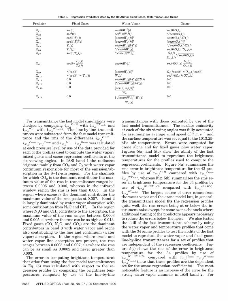
The functional dependence of the predictors Xj,kused to parameterize the optical depth dn*, j9 dependsmainly on factors such as the absorbing gas, ISRF,and spectral region although the order in which thegases are separated out @Eqs. ~11! and ~12!# and thelayer thickness can also be important. The predic-tors Xj,k that we used in this paper are based, withmodifications, on those selected for the AtmosphericInfrared Sounder ~AIRS! fast transmittance mod-el19,37 given that most of the problems posed by find-ing an optimal set of predictors that work well for thethousands of channels of an instrument such as AIRSwere also expected to be encountered for an instru-ment such as the IASI with its 8461 channels. Themost basic predictors ~all defined in Table 2! are de-
ned from the ratios Tr~ j!, Wr~ j!, Or~ j! and from thedifferences dT~ j!. This is because within the frame-work of a linear regression method the great variabil-
aThe pres~l !’s are the values of the pressure at each level. Tprofile~l !, Wprofile~l !, and Oprofile~l ! are the temperature, water vapor mixingratio, and ozone mixing ratio profiles. Treference~l !, Wreference~l !, and Oreference~l ! are the corresponding reference profiles. For thesevariables l refers to the lth level; otherwise l is the lth layer, i.e., the layer above the lth level. Note that we take P~0! 5 2P~1! 2 P~2!.Also Tw~1! 5 0 and OTw~1! 5 0.
tpba
nlmptw
ct
md
co2
ity between extreme profiles makes the regressionprone to numerical instabilities and thus difficultiesin calculating the coefficients can arise if the predic-tors are allowed to vary too much. Simple functionsinvolving combinations of the basic predictors and ofthe viewing angle can account for the behavior of thelayer optical depth of a gas treated as having thetransmittance properties of a gas in a homogeneouslayer at pressure P, temperature T, and absorberamount n. This can be accurate for monochromaticransmittances but in practice we have to predictolychromatic transmittances and additional termsased on those given by Fleming and McMillin14 aredded. These are the predictors Tw~l !, Ww~l !, Ow~l !.
These predictors account for the dependence of thelayer transmittance on the properties of the atmo-sphere above the layer. Note that, although the useof Eqs. ~9!, ~10!, and ~11! reduces this dependence,
evertheless, for a temperature sounding channel theayer transmittance for two profiles having the same
ean layer temperature but different temperaturerofiles over the actual layer will still differ in thathe profile with greater optical depth above the layerill have a smaller optical depth within the layer.The final form of the IASI predictors was defined
arrying out trials in which some changes were madeo the AIRS fast transmittance model predictors.19,37
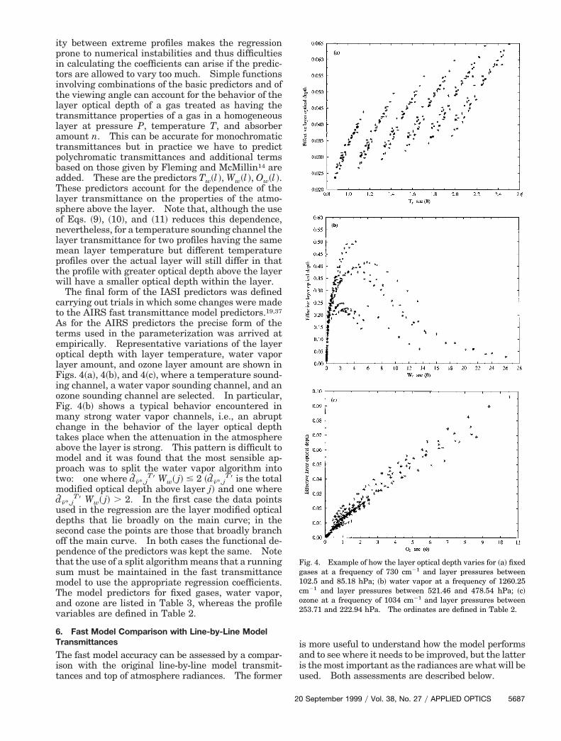
As for the AIRS predictors the precise form of theterms used in the parameterization was arrived atempirically. Representative variations of the layeroptical depth with layer temperature, water vaporlayer amount, and ozone layer amount are shown inFigs. 4~a!, 4~b!, and 4~c!, where a temperature sound-ing channel, a water vapor sounding channel, and anozone sounding channel are selected. In particular,Fig. 4~b! shows a typical behavior encountered inmany strong water vapor channels, i.e., an abruptchange in the behavior of the layer optical depthtakes place when the attenuation in the atmosphereabove the layer is strong. This pattern is difficult tomodel and it was found that the most sensible ap-proach was to split the water vapor algorithm intotwo: one where dn*, j
T9 Ww~ j! # 2 ~dn*, jT9 is the total
odified optical depth above layer j! and one whereˆ
n*, jT9 Ww~ j! . 2. In the first case the data points
used in the regression are the layer modified opticaldepths that lie broadly on the main curve; in thesecond case the points are those that broadly branchoff the main curve. In both cases the functional de-pendence of the predictors was kept the same. Notethat the use of a split algorithm means that a runningsum must be maintained in the fast transmittancemodel to use the appropriate regression coefficients.The model predictors for fixed gases, water vapor,and ozone are listed in Table 3, whereas the profilevariables are defined in Table 2.
6. Fast Model Comparison with Line-by-Line ModelTransmittances
The fast model accuracy can be assessed by a compar-ison with the original line-by-line model transmit-tances and top of atmosphere radiances. The former
20
is more useful to understand how the model performsand to see where it needs to be improved, but the latteris the most important as the radiances are what will beused. Both assessments are described below.
Fig. 4. Example of how the layer optical depth varies for ~a! fixedgases at a frequency of 730 cm21 and layer pressures between102.5 and 85.18 hPa; ~b! water vapor at a frequency of 1260.25m21 and layer pressures between 521.46 and 478.54 hPa; ~c!zone at a frequency of 1034 cm21 and layer pressures between53.71 and 222.94 hPa. The ordinates are defined in Table 2.
September 1999 y Vol. 38, No. 27 y APPLIED OPTICS 5687
maFcavwrc0
tigp
tfaf
rfi
sns
Table 3. Regression Predictors Used by the RTIASI for Fixed Gases, Water Vapor, and Ozone
5
For transmittance the fast model simulations werechecked by comparing tn*, j
F1W with tn*, jWVmodel and
tn*, j~O!9 with tn*, j
~O!model. The line-by-line transmit-tances were subtracted from the fast model transmit-tance and the rms of the differences tn*, j
F1W 2tn*, j
Fmodel tn*,jWmodel and tn*, j
O9 2 tn*,jOmodel was calculated
at each pressure level by use of the data provided foreach of the profiles used to compute the water vaporymixed gases and ozone regression coefficients at thesix viewing angles. In IASI band 1 the radiancesoriginate mainly from CO2 and O3 with water vaporcontinuum responsible for most of the emissionyab-sorption in the 8–12-mm region. For the channelsfor which CO2 is the dominant contributor the max-imum value of the rms in transmittance ranges be-tween 0.0005 and 0.006, whereas in the infraredwindow region the rms is less than 0.005. In theregion where ozone is the dominant contributor themaximum value of the rms peaks at 0.007. Band 2is largely dominated by water vapor absorption withsome contribution from N2O and CH4. In the regionwhere N2O and CH4 contribute to the absorption, the
aximum value of the rms ranges between 0.0003nd 0.005, elsewhere the rms can be as high as 0.013.ixed gases ~CO, N2O, and CO2! are the dominantontributors in band 3 with water vapor and ozonelso contributing to the line and continuum ~waterapor! absorption. In the region where ozone andater vapor line absorption are present, the rms
anges between 0.0005 and 0.007; elsewhere the rmsan be as small as 0.0002 and never greater than.003.The error in computing brightness temperatures
hat arise from using the fast model transmittancesn Eq. ~5! was calculated with respect to the re-ression profiles by comparing the brightness tem-eratures computed by use of the line-by-line
688 APPLIED OPTICS y Vol. 38, No. 27 y 20 September 1999
ransmittances with those computed by use of theast model transmittances. The surface emissivityt each of the six viewing angles was fully accountedor assuming an average wind speed of 7 m s21 and
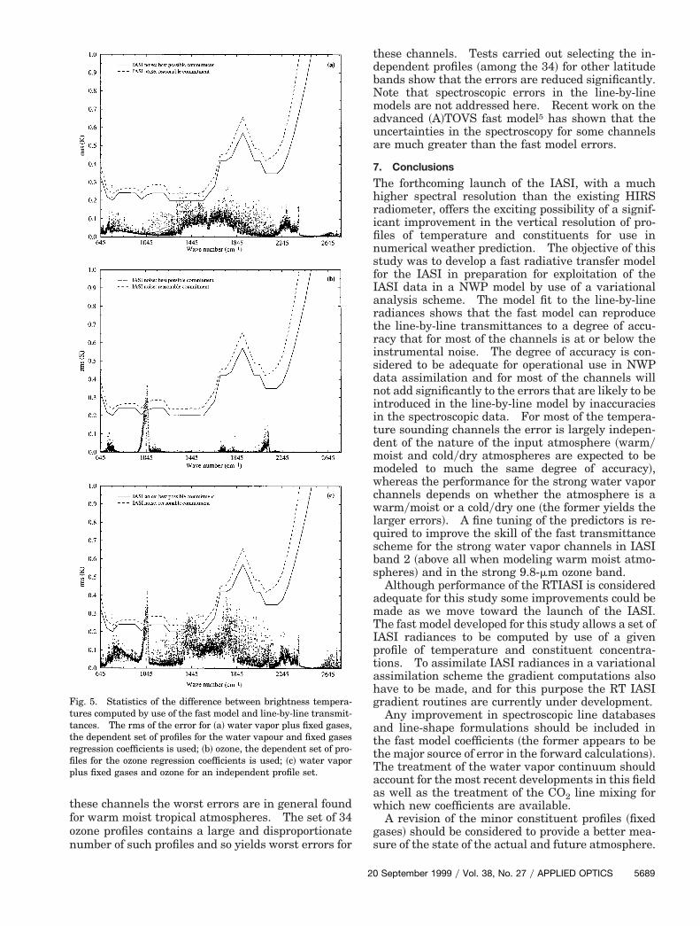
the surface temperature was set equal to the 1013.25-hPa air temperature. Errors were computed forozone alone and for fixed gases plus water vapor.Figures 5~a! and 5~b! show the ability of the fasttransmittance model to reproduce the brightnesstemperatures for the profiles used to compute theregression coefficients. Figure 5~a! summarizes thems error in brightness temperature for the 43 pro-les by use of tn*, j
F1W compared with tn*, jFmodel
tn*, jWVmodel, whereas Fig. 5~b! summarizes the rms er-
ror in brightness temperature for the 34 profiles byuse of tn*, j
~F1WV1O! compared with tn*, j~F1WV!9
tn*, j~O!model. The largest source of error comes from
the water vapor and the ozone model but, in general,the transmittance model fits the regression profilesquite well, the rms errors being at or below the in-strument noise except for some ozone channels whereadditional tuning of the predictors appears necessaryto reduce the errors below the noise. We also testedthe skill of the fast transmittance scheme by usingthe water vapor and temperature profiles that comewith the 34 ozone profiles to test the ability of the fastmodel to reproduce the water vapor and fixed gasesline-by-line transmittances for a set of profiles thatare independent of the regression coefficients. Fig-ure 5~c! shows the rms of the error in brightnesstemperature for the 34 profiles by use oftn*, j
~F1WV1O!9 compared with tn*, jFmodel tn*, j
WVmodel
tn*, jOmodel ~note that these profiles are the dependent
et for the ozone regression coefficients!. The mostoticeable feature is an increase of the error for thetrong water vapor channels in IASI band 2. For
these channels the worst errors are in general foundfor warm moist tropical atmospheres. The set of 34ozone profiles contains a large and disproportionatenumber of such profiles and so yields worst errors for
20
these channels. Tests carried out selecting the in-dependent profiles ~among the 34! for other latitudebands show that the errors are reduced significantly.Note that spectroscopic errors in the line-by-linemodels are not addressed here. Recent work on theadvanced ~A!TOVS fast model5 has shown that theuncertainties in the spectroscopy for some channelsare much greater than the fast model errors.
7. Conclusions
The forthcoming launch of the IASI, with a muchhigher spectral resolution than the existing HIRSradiometer, offers the exciting possibility of a signif-icant improvement in the vertical resolution of pro-files of temperature and constituents for use innumerical weather prediction. The objective of thisstudy was to develop a fast radiative transfer modelfor the IASI in preparation for exploitation of theIASI data in a NWP model by use of a variationalanalysis scheme. The model fit to the line-by-lineradiances shows that the fast model can reproducethe line-by-line transmittances to a degree of accu-racy that for most of the channels is at or below theinstrumental noise. The degree of accuracy is con-sidered to be adequate for operational use in NWPdata assimilation and for most of the channels willnot add significantly to the errors that are likely to beintroduced in the line-by-line model by inaccuraciesin the spectroscopic data. For most of the tempera-ture sounding channels the error is largely indepen-dent of the nature of the input atmosphere ~warmymoist and coldydry atmospheres are expected to bemodeled to much the same degree of accuracy!,whereas the performance for the strong water vaporchannels depends on whether the atmosphere is awarmymoist or a coldydry one ~the former yields thelarger errors!. A fine tuning of the predictors is re-quired to improve the skill of the fast transmittancescheme for the strong water vapor channels in IASIband 2 ~above all when modeling warm moist atmo-pheres! and in the strong 9.8-mm ozone band.Although performance of the RTIASI is considered
adequate for this study some improvements could bemade as we move toward the launch of the IASI.The fast model developed for this study allows a set ofIASI radiances to be computed by use of a givenprofile of temperature and constituent concentra-tions. To assimilate IASI radiances in a variationalassimilation scheme the gradient computations alsohave to be made, and for this purpose the RT IASIgradient routines are currently under development.
Any improvement in spectroscopic line databasesand line-shape formulations should be included inthe fast model coefficients ~the former appears to bethe major source of error in the forward calculations!.
he treatment of the water vapor continuum shouldccount for the most recent developments in this fields well as the treatment of the CO2 line mixing for
which new coefficients are available.A revision of the minor constituent profiles ~fixed
gases! should be considered to provide a better mea-sure of the state of the actual and future atmosphere.
Fig. 5. Statistics of the difference between brightness tempera-tures computed by use of the fast model and line-by-line transmit-tances. The rms of the error for ~a! water vapor plus fixed gases,the dependent set of profiles for the water vapour and fixed gasesregression coefficients is used; ~b! ozone, the dependent set of pro-files for the ozone regression coefficients is used; ~c! water vaporplus fixed gases and ozone for an independent profile set.
September 1999 y Vol. 38, No. 27 y APPLIED OPTICS 5689
15. L. M. McMillin, H. E. Fleming, and M. L. Hill, “Atmospheric
5
In this respect some fixed gases could be allowed tovary by use of a parameterization of the same type asthat used for the variable gases.
Finally, for the shorter wavelengths a solar contri-bution term could be added to the simulated radianceand the treatment of the reflected thermal term inthe RT equation could be improved from the currentapproximate formulation.
This research was supported by EUMETSAT con-tract EUMyCOy96y389yDD. Many individualshave contributed to this study. We particularly ac-knowledge the useful discussions with R. Rizzi, Uni-versita’ di Bologna; L. Strow, University of Maryland;P. Rayer, U.K. Meteorological Office; F. Cayla, CentreNational d’Etudes Spatiales; and S. J. Evans, Impe-rial College.
3. J. R. Eyre, G. A. Kelly, A. P. McNally, E. Anderson, and A.Persson, “Assimilation of TOVS radiance information throughone-dimensional variational analysis,” Q.J.R. Meteorol. Soc.119, 1427–1463 ~1993!.
4. F. Rabier, J. Thepaut and P. Courtier, “Extended assimilationand forecast experiments with a four dimensional variationalassimilation system,” Q.J.R. Meteorol. Soc. 124, 1861–1887~1998!.
5. R. Saunders, M. Matricardi, and P. Brunel, “An improved fastradiative transfer model for assimilation of satellite radianceobservations,” Q.J.R. Meteorol. Soc. 125, 1407–1425 ~1999!.
6. L. M. McMillin, L. J. Crone, M. D. Goldberg, and T. J.Kleespies, “Atmospheric transmittances of an absorbing gas.4. OPTRAN: a computationally fast and accurate transmit-tance model for absorbing gases with fixed and with variablemixing ratios at variable viewing angles,” Appl. Opt. 34, 6269–6274 ~1995!.
7. L. M. McMillin, L. J. Crone, and T. J. Kleespies, “Atmospherictransmittance of an absorbing gas. 5. Improvements to theOPTRAN approach,” Appl. Opt. 34, 8396–8399 ~1995!.
8. J. R. Eyre, “A fast radiative transfer model for satellite sound-ing systems,” ECMWF Research Department Technical Mem-orandum 176 ~European Centre for Medium-Range WeatherForecasts, Reading, UK, 1991!.
9. R. M. Goody and Y. L. Yung, Atmospheric Radiation: Theo-retical Basis ~Oxford University, New York, 1995!.
10. K. Masuda, T. Takashima, and T. Takayama, “Emissivity ofpure sea waters for the model sea surface in the infraredwindow regions,” Remote Sens. Environ. 24, 313–329 ~1988!.
11. G. M. Hale and M. R. Querry, “Optical constants of water inthe 200-nm to 200-mm wavelength region,” Appl. Opt. 12, 555–563 ~1973!.
12. D. Friedman, “Infrared characteristics of ocean water ~1.5–15mm!,” Appl. Opt. 8, 2073–2078 ~1969!.
13. L. M. McMillin and H. E. Fleming, “Atmospheric transmit-tance of an absorbing gas: a computationally fast and accu-rate transmittance model for absorbing gases with constantmixing ratios in inhomogeneous atmospheres,” Appl. Opt. 15,358–363 ~1976!.
14. H. E. Fleming and L. M. McMillin, “Atmospheric transmit-tance of an absorbing gas. 2. A computationally fast andaccurate transmittance model for slant paths at different ze-nith angles,” Appl. Opt. 16, 1366–1370 ~1977!.
690 APPLIED OPTICS y Vol. 38, No. 27 y 20 September 1999
transmittances of an absorbing gas. 3: A computationallyfast and accurate transmittance model for absorbing gaseswith variable mixing ratios,” Appl. Opt. 18, 1600–1606 ~1979!.
16. J. Susskind, J. Rosenfeld, and D. Reuter, “An accurate radia-tive transfer model for use in the direct physical inversion ofHIRS2 and MSU temperature sounding data,” J. Geophys.Res. 88, 8550–8568 ~1983!.
17. J. R. Eyre and H. M. Woolf, “Transmittance of atmosphericgases in the microwave region: a fast model,” Appl. Opt. 27,3244–3249 ~1988!.
18. P. J. Rayer, “Fast transmittance model for satellite sounding,”Appl. Opt. 34, 7387–7394 ~1995!.
19. S. E. Hannon, L. L. Strow, and W. W. McMillan, “Atmosphericinfrared fast transmittance models: a comparison of two ap-proaches,” in Optical Spectroscopic Techniques and Instrumen-tation for Atmospheric and Space Research II, P. B. Hays andJ. Wang, eds., Proc. SPIE 2830, 94–105 ~1996!.
20. A. Chedin, N. A. Scott, C. Wahiche, and P. Moulnier, “Theimproved initialization inversion method: a high resolutionphysical method for temperature retrievals from satellites ofthe TIROS-N series,” J. Clim. Appl. Meteorol. 24, 128–143~1985!.
21. R. Rizzi, Dipartimento di Fisica Universita’ di Bologna, Bolo-gna, Italy ~personal communication, 1996!.
22. S. J. Evans, Imperial College, London, UK ~personal commu-nication, 1997!.
23. J. E. Harries, J. M. Russel, A. F. Tuck, L. L. Gordley, P.Purcell, K. Stone, R. M. Bevilacqua, M. Gunson, G. Nedoluha,and W. A. Traub, “Validation of measurements of water vapourfrom the Halogen Occultation Experiment ~HALOE!,” J. Geo-phys. Res. 101, 10,205–10,216 ~1996!.
24. D. P. Edwards, “GENLN2. A general line-by-line atmo-spheric transmittance and radiance model,” NCAR Technicalnote NCARyTN-3671STR ~National Center for AtmosphericResearch, Boulder, Colo., 1992!.
25. L. S. Rothman, C. P. Rinsland, A. Goldman, S. T. Massie, D. P.Edwards, J.-M. Flaud, A. Perrin, C. Camy-Peyret, V. Dana,J.-Y. Mandin, J. Schroeder, A. McCann, R. R. Gamache, R. B.Watson, K. Yoshino, K. V. Chance, K. W. Jucks, L. R. Brown,V. Nemtchinov, and P. Varanasi, “The HITRAN molecularspectroscopic database and HAWKS (HITRAN AtmosphericWorkstation!: 1996 edition,” J. Quant. Spectrosc. Radiat.Transfer 60, 665–710 ~1998!.
26. B. H. Armstrong, “Spectrum line profiles: the Voigt function,”J. Quant. Spectrosc. Radiat. Transfer 7, 66–88 ~1967!.
27. L. L. Strow, D. C. Tobin, and S. E. Hannon, “A compilation offirst-order line-mixing coefficients for CO2 Q-branches,” J.Quant. Spectrosc. Radiat. Transfer 52, 281–294 ~1994!.
28. S. A. Clough, F. X. Kneizys, R. Davies, R. Gamache, and R.Tipping, “Theoretical line shape for H2O vapour: applicationto the continuum,” in Atmospheric Water Vapour, A Deepak,T. D. Wilkerson, and L. H. Ruhnke, eds. ~Academic, New York,1980!, pp. 25–46.
29. S. A. Clough, F. X. Kneizys, and R. W. Davis, “Line shape andthe water vapour continuum,” Atmos. Res. 23, 229–241 ~1989!.
30. S. A. Clough, F. X. Kneizys, L. S. Rothman, and W. O. Gallery,“Atmospheric spectral transmission and radiance:FASCOD1B,” in Atmospheric Transmission, R. W. Fenn, ed.,Proc. SPIE 277, 152–166 ~1981!.
31. V. Menoux, R. Le Doucen, C. Boulet, A. Roblin, and A. M.Bouchardy, “Collision-induced absorption in the fundamentalband of N2: temperature dependence of the absorption forN2–N2 and N2–O2 pairs,” Appl. Opt. 32, 263–268 ~1993!.
32. Y. M. Timofeyev and M. V. Tonkov, “Effect of the inducedoxygen absorption band on the transformation of radiation inthe 6 mm region of the Earth’s atmosphere,” Izv. Acad. Sci.USSR Atmos. Oceanic Phys. 14, 437–441 ~1978!.
33. C. P. Rinsland, J. S. Zander, J. S. Namkung, C. B. Farmer, and Change, J. T. Houghton, L. G. Meira Filho, B. A. Callander, N.
3
R. H. Norton, “Stratospheric infrared continuum absorptionobserved by the ATMOS instrument,” J. Geophys. Res. 94,16,303–16,322 ~1989!.
34. D. Schimel, D. Alves, I. Enting, M. Heiman, F. Joos, D.Raynaud, T. Wigley, M. Prather, R. Derwent, D. Ehalt, P.Fraser, E. Sanhueza, X. Zhou, P. Jonas, R. Charlson, H. Rodhe,S. Sadasivan, K. P. Shine, Y. Fouquart, V. Ramaswamy, S.Solomon, J. Srinivasan, D. Albritton, R. Derwent, I. Isaksen,M. Lal, and D. Wuebbles, “Radiative forcing of climatechange,” in Climate Change 1995: the Science of Climate
20
Harris, A. Kattenberg, and K. Maskell, eds. ~Cambridge Uni-versity, Cambridge, UK, 1996!, pp. 69–131.
5. F. Cayla, “Simulation of IASI spectra,” CNES document IA-TN-0000-5627-CNE ~Centre National D’ Etudes Spatiales,Toulouse, France, 1996!.
36. E. O. Brigham, Fast Fourier Transform ~Prentice-Hall, Engle-wood Cliffs, N.J., 1974!.
37. L. L. Strow, University of Maryland, Baltimore County 1000Hilltop Circle, Baltimore, Md. 21250 ~personal communica-tion, 1998!.
September 1999 y Vol. 38, No. 27 y APPLIED OPTICS 5691