150 TRANSPORTATION RESEARCH RECORD 1286 Fatigue Damage Properties of Asphaltic Concrete Pavements Kuo-HUNG TSENG AND ROBERT L. LYTTON The development of material property relations for the two fatigue damage properties, K 1 and K 2 , which can be used to predict the fatigue life of asphaltic concrete pavements, is described. The fatigue damage properties developed are based on the theory of fracture mechanics along with regression analysis on published beam fatigue data and, thus, can take into account crack initia- tion, propagation, and material properties that are not accounted for with the conventional strain-based fatigue equation. The approach provides more insight into how these fatigue damage properties reflect the fatigue behavior of asphaltic concrete pave- ment while producing acceptable estimates of field fatigue life. Derivations have shown that the fatigue damage property K 1 is dependent on the asphalt mixture and pavement properties, such as the parameters of the Paris crack growth law , elastic stiffness , and thickness of the asphaltic concrete layer and that the fatigue damage property K 2 varies with the initial asphalt cement prop- erties, such as asphalt content, viscosity, penetration, and tem- perature. Two significant functions of the fatigue damage prop- erties developed are (a) the prediction of fatigue life allows for the application of loading with single or dual tires on single, tandem, or triple axles, and (b) they provide for the calculation of load equivalence factors for fatigue life as affected by multiple- axle loads. A shift factor that can be used to adjust the laboratory (or calculated) fatigue damage properties to that measured in the field is also described. This factor takes into account healing and residual stresses between applications of traffic loads that are responsible for the difference in fatigue life between laboratory test results and those measured in the field. FATIGUE DAMAGE PROPERTIES OF ASPHALTIC CONCRETE PAVEMENTS The evaluation of fatigue cracking caused by repeated loads is important in the design and prediction of the service life of flexible pavements. The procedure conventionally used for predicting fatigue life is based on the "phenomenological approach," in which, commonly, the fatigue life is measured by laboratory testing with a third-point flexural load applied on a beam under controlled stress or strain conditions at a given temperature and frequency. The fatigue results thus obtained from laboratory tests are expressed as a power law relation between the tensile strain ( i:) in the bottom of the beam and the number of load applications to failure N 1 . The relation is given by (1) K-H. Tseng, Texas Transportation Institute, Texas A&M University Systems, College Station, Tex. 77843 . R. L. Lytton, Civil Engineer- ing Department, Texas A&M University, College Station, Tex. 77843. where K 1 and K 2 are the phenomenological regression con- stants. Once K 1 and K 2 are obtained from laboratory tests, the fatigue life of asphaltic concrete pavement can be esti- mated from Equation 1. A number of laboratory studies (1 ,2) have shown that these constants are affected by material prop- erties such as mixture stiffness, air voids, asphalt content, viscosity of asphalt cement, and gradation of the aggregate; by the dimensions of the test sample; and by environmental conditions, such as the temperature during the tests. This information indicates that a more profound understanding is needed of how these two constants, K 1 and K 2 , depend on the fatigue behavior and material properties of an asphaltic concrete mix. The objective of this paper is to present the development of the fatigue damage properties of asphaltic concrete pave- ments by applying the theory of fracture mechanics to the results of laboratory beam fatigue tests. The prediction of fatigue life based on the fatigue damage properties that are developed also allows for the application of loading with single or dual tires on single, tandem, or triple axles. This devel- opment, subsequently, provides for the calculation of load equivalence factors for fatigue life as affected by multiple- axle loads. Along with the fatigue damage properties, a shift factor is described that takes into account the effects of healing and residual stress between applications of traffic loads and can be used to adjust the laboratory (or calculated) fatigue damage properties to that observed in the field. The complete procedures for predicting fatigue life based on the fatigue damage properties have been included in the FEPASS (Finite Element Performance Analysis Structural Subsystem) computer program (3), which is a revised version ofILLl-PAVE (4) . The FEPASS program also has the ability to predict the rutting and loss of serviceability index of inser- vice payments, taking into account realistic distributions of tire contact pressure, both vertical and horizontal, and has the ability to provide various amounts of resistance to slip between layers. This paper is organized to present a better understanding of fatigue characterization of asphaltic concrete pavements. Other applications of the FEP ASS program are presented elsewhere (3). · DEVELOPMENT OF RELATION BETWEEN FATIGUE EQUATION AND CRACK GROWTH LAW Utilizing Paris' crack growth law (5), the number of load cycles (N 1 ) can be expressed as
Transcript
150 TRANSPORTATION RESEARCH RECORD 1286
Fatigue Damage Properties of Asphaltic Concrete Pavements
Kuo-HUNG TSENG AND ROBERT L. LYTTON
The development of material property relations for the two fatigue damage properties, K1 and K2, which can be used to predict the fatigue life of asphaltic concrete pavements, is described. The fatigue damage properties developed are based on the theory of fracture mechanics along with regression analysis on published beam fatigue data and, thus, can take into account crack initiation, propagation, and material properties that are not accounted for with the conventional strain-based fatigue equation. The approach provides more insight into how these fatigue damage properties reflect the fatigue behavior of asphaltic concrete pavement while producing acceptable estimates of field fatigue life. Derivations have shown that the fatigue damage property K1 is dependent on the asphalt mixture and pavement properties, such as the parameters of the Paris crack growth law, elastic stiffness , and thickness of the asphaltic concrete layer and that the fatigue damage property K2 varies with the initial asphalt cement properties, such as asphalt content, viscosity, penetration, and temperature. Two significant functions of the fatigue damage properties developed are (a) the prediction of fatigue life allows for the application of loading with single or dual tires on single, tandem, or triple axles, and (b) they provide for the calculation of load equivalence factors for fatigue life as affected by multipleaxle loads. A shift factor that can be used to adjust the laboratory (or calculated) fatigue damage properties to that measured in the field is also described. This factor takes into account healing and residual stresses between applications of traffic loads that are responsible for the difference in fatigue life between laboratory test results and those measured in the field.
FATIGUE DAMAGE PROPERTIES OF ASPHALTIC CONCRETE PAVEMENTS
The evaluation of fatigue cracking caused by repeated loads is important in the design and prediction of the service life of flexible pavements. The procedure conventionally used for predicting fatigue life is based on the "phenomenological approach," in which , commonly, the fatigue life is measured by laboratory testing with a third-point flexural load applied on a beam under controlled stress or strain conditions at a given temperature and frequency. The fatigue results thus obtained from laboratory tests are expressed as a power law relation between the tensile strain ( i:) in the bottom of the beam and the number of load applications to failure N1. The relation is given by
(1)
K-H. Tseng, Texas Transportation Institute, Texas A&M University Systems, College Station, Tex. 77843. R. L. Lytton, Civil Engineering Department, Texas A&M University, College Station, Tex. 77843.
where K1 and K 2 are the phenomenological regression constants. Once K1 and K2 are obtained from laboratory tests, the fatigue life of asphaltic concrete pavement can be estimated from Equation 1. A number of laboratory studies (1 ,2) have shown that these constants are affected by material properties such as mixture stiffness, air voids, asphalt content, viscosity of asphalt cement, and gradation of the aggregate; by the dimensions of the test sample; and by environmental conditions, such as the temperature during the tests . This information indicates that a more profound understanding is needed of how these two constants, K1 and K2 , depend on the fatigue behavior and material properties of an asphaltic concrete mix .
The objective of this paper is to present the development of the fatigue damage properties of asphaltic concrete pavements by applying the theory of fracture mechanics to the results of laboratory beam fatigue tests. The prediction of fatigue life based on the fatigue damage properties that are developed also allows for the application of loading with single or dual tires on single, tandem, or triple axles. This development, subsequently, provides for the calculation of load equivalence factors for fatigue life as affected by multipleaxle loads. Along with the fatigue damage properties, a shift factor is described that takes into account the effects of healing and residual stress between applications of traffic loads and can be used to adjust the laboratory (or calculated) fatigue damage properties to that observed in the field.
The complete procedures for predicting fatigue life based on the fatigue damage properties have been included in the FEPASS (Finite Element Performance Analysis Structural Subsystem) computer program (3), which is a revised version ofILLl-PAVE (4) . The FEPASS program also has the ability to predict the rutting and loss of serviceability index of inservice payments, taking into account realistic distributions of tire contact pressure , both vertical and horizontal , and has the ability to provide various amounts of resistance to slip between layers. This paper is organized to present a better understanding of fatigue characterization of asphaltic concrete pavements. Other applications of the FEP ASS program are presented elsewhere (3). ·
DEVELOPMENT OF RELATION BETWEEN FATIGUE EQUATION AND CRACK GROWTH LAW
Utilizing Paris' crack growth law (5), the number of load cycles (N1) can be expressed as
Tseng and Lytton
(2)
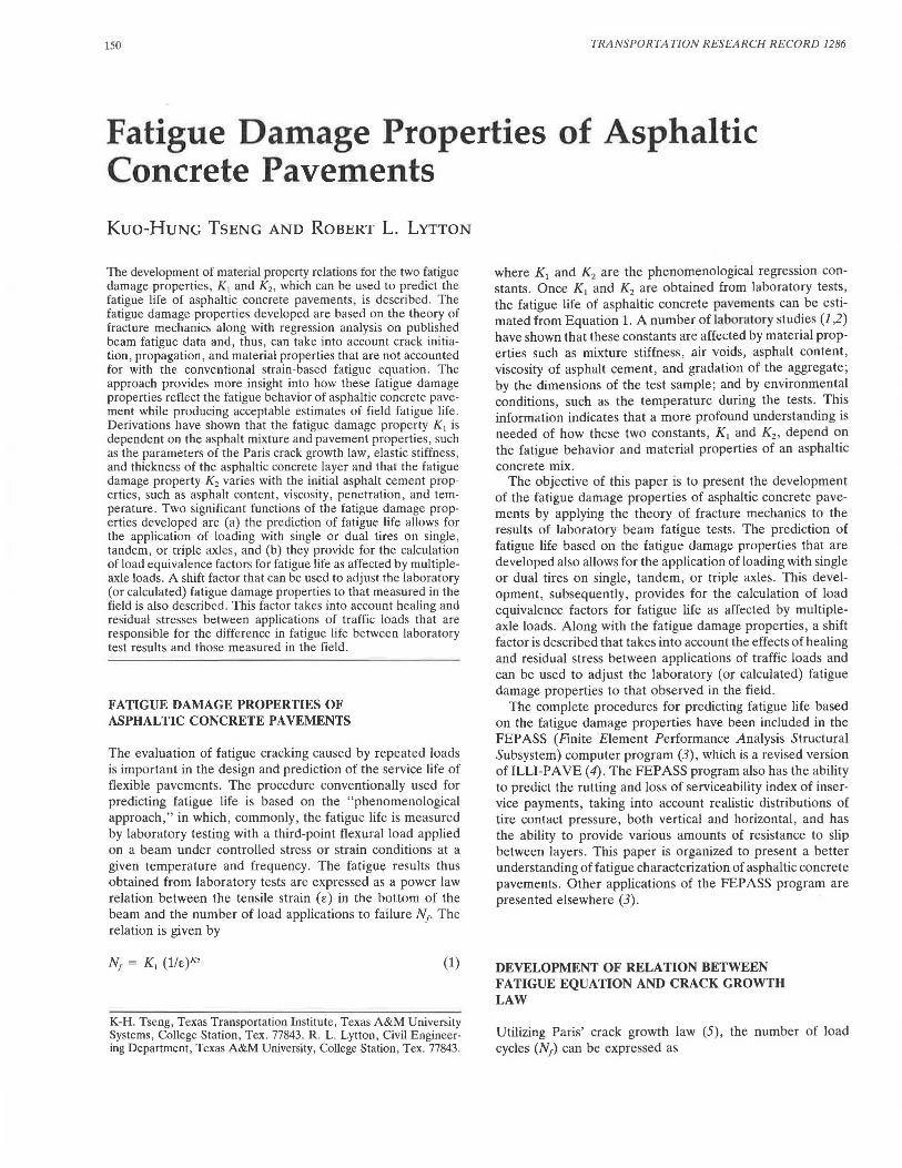
where C0 is initial crack length, C1 is final crack length, A and n are the fracture parameters, and tlK is the difference of the stress intensity factor that occurs at the tip of the crack during the passage of a load. In addition to the fracture parameters in Paris' equation, the stress intensity factor caused by the loading conditions and initial crack tip geometry are also required to develop equations that model pavement fatigue life. A finite element computer program is used to evaluate stress intensity factors induced within both the laboratory fatigue beam and the asphaltic concrete layer in pavements. The program, which was originally developed for plane stress or plane strain analysis by Desai and Abel (6) was subsequently modified by Jayawickrama (7) to allow for the use of the energy release method for evaluating stress intensity factors. The stress intensity factors are then computed for various crack-tip positions. The computed data for an elastic beam fatigue test are reduced to nondimensional form as shown in Figure 1 and are represented by the expression
K (c)q d112u=r d (3)
where
151
u = maximum stress at extreme fiber of the beam ( = EE),
E = the elastic stiffness of the fatigue beam corresponding to the loading frequency and temperature,
E = the tensile strain at the extreme fiber of the beam,
c = crack length, d = depth of the beam, and
r and q = regression constants; r = 4.397, q = 1.180.
A laboratory method that measures the fracture properties and the strain energy release rate directly is presently in use (8). This method, which is known as the J-integral method, is applicable to all materials, regardless of their constitutive equations. There are no mechanistic methods available to calculate the J-integral strain energy release rate for pavements in the field, however; thus laboratory methods-although they are applicable to all materials-must remain confined to laboratory applications for the moment, and the linear elastic fracture mechanics method presented here is the only laboratory method for which a mechanistic pavement model is currently available for field applications.
FIGURE 1 Determination of stress intensity factor for various cracktip positions.
152
Substituting the stress intensity factor from Equation 3 into Equation 2, the fatigue life (N1) becomes
(4)
The initial crack length ( C0) is estimated to be the radius of the largest aggregate particle. This estimation is based on laboratory observations. The fracture coefficients A and n are determined from laboratory tests as the intercept and slope , respectively, on a log-log plot of stress intensity factor (K) versus the rate of crack growth (daldN). Equation 4 is identical to Equation 1, which is used to describe the fatigue characterization based on the controlled-strain mode in the laboratory. Therefore, the fatigue damage properties (K1 and K 2) of the fatigue equation can be calculated from
1-~ [ (C0)
1-"q] d 2 1 - -d
K1 = ---------A (1 - nq) (Er)"
(5)
and
(6)
It is apparent from Equation 5 that log K 1 depends in a complex way on K2 (or n). The empirical observation of a "linear relation" of the two variables is thus shown to be theoretically incorrect, although a plot of log K 1 versus n using Equation 5 normally produces a nearly linear relation. This points up the value of having a theory: the relation in Equation 5 could not have been discovered by using regression analysis .
In addition to the A and n values obtained from laboratory tests, a theoretical equation of crack growth derived by Schapery (9) also can be used to calculate these two parameters. Experimental studies (10) on asphaltic concrete mixes to verify Schapery's equation have shown that the value of n is evaluated by the following relationship, which is derived from theory:
n = 2/m (7)
where m is the slope of the tensile creep compliance curve obtained from laboratory creep tests. However, the value of m in this paper is determined alternatively from the straightline portion of the log-log plot on the mix stiffness versus loading time at the test temperature. A computerized version of the McLeod nomograph (11) has been developed by Jayawickrama et al. (12) to calculate the values of m and n when creep compliance and other material properties are not available. This program requires input information of (a) penetration at 77°F, (b) viscosity at 275°F or at 140°F, (c) service temperature, (d) asphalt content, and (e) air void content. Alternatively, the same m and n may be calculated using the Van der Poe! nomograph (13-15) if the ring-and-ball softening point and penetration are available.
Theoretically, based on Schapery's equation, the value of A can be calculated from those variables such as creep compliance, Poisson's ratio, fracture energy, tensile strength, shape
TRA NSPORTA TION RESEARCH RECORD 1286
of the loading stress pulse, and other factors. The calculation of A by means of Schapery's equation is complicated by the fact that not all of the variables that are required to calculate the value of A in the equation were measured in previously published beam fatigue tests. Data from a total of 32 published beam fatigue tests were collected from three different sources (16-18) and are shown in Table 1. A regression equation for estimating A was developed from the data that were available.
In Equation 5, the parameter A can be rearranged as
A
1-~ [ (C0 )
1-"q] d 2 1 - -d
(8) K1(l - nq)(Er)"
The value of n and E in Equation 8 are the actual observed K2 , and observed elastic stiffness, respectively, and each value of A is then back calculated from the available 32 beam fatigue test results. The regression analysis is made by using the parameter A as the dependent variable and the observed K2 ,
observed elastic stiffness, loading frequency, and specimen size as the independent variables. It is found that the value of A is best explained in terms of the exponent K2 and the elastic stiffness of the mix . The regression equation for A is then developed:
log A = 7.0889 - 2.4755 K 2 (9) - 2.1163 log E R2 = 0.86
Thus, to use Equation 9 for the estimation of A, the flexural elastic stiffness (E) is calculated from the McLeod-Van der Poe! routine (11,13), and K 2 is equal ton, which is calculated from 2/m. The value of m is also calculated with the McLeodVan der Poe! routine . Once the value of A is estimated and mis obtained, the fatigue damage properties (K1 and K2) can be evaluated by using Equations 5 and 6.
COMPARISONS OF CALCULATED AND EXPERIMENTAL K1 AND K2 AND ELASTIC STIFFNESS
As described previously, it has been shown that the exponent (K2) of the fatigue relation and the exponent (n) of the crack growth law are equal to each other. Also shown is that the constant K 1 of the fatigue relation is an explicit function of several material properties, including the exponent of the crack growth law and the size of specimen. It is of interest whether these conclusions agree with the experimental results.
The computation of the slope m of the available 32 laboratory data is carried out by using a computerized version of the Van der Poe! nomograph (13) and modified by Heukelom and Klomp (14). This program was originally developed by DeBats (15) and is named PONOS. It has been modified to calculate the information that is necessary to determine the fatigue parameters of a mix, such as the values of m and n. Because the data of Kallas and Puzinauskas do not have the ring-and-ball softening point information that is required in the PONOS program, an alternative computerized version of McLeod's nomograph is used to calculate these fatigue param-
Tseng and Lytton 153
TABLE 1 FATIGUE TESTING DATA
Mb: Type
Aaph•ll Vlocoolt:r Contenl •l 140 "F
Penetr•Uon "•l 77 °F
Rl£B Sonenlng Pl.
Air Vold
Temp ·r
Freq
Ho Mn:. Sin
Sllff'neH lml
K, K,
Eppo Brili!h 594
Sanlucci AC
Kan .. AC Sur(ac•
1.9 6.0
6.0 6.0 6.0
6.l 5.9
6.0
5.9 5.9 5.9 5.9 4.9 4.9 4.9 4.9
4.9 4.9 4.9 4.9
6.0 6.0
6.0 6.0 6.0
6.0
5.6 5.7
5.l 6.0 6.0 6.0
2840 1760 lllD 2670 2670 2670
21 36
JO
J7 JS
26 JS
48
57 41 25 J8 J8
26 28 28 J2
28 JO 20
18 IJ
8.5
21 JO 26
57 84
90
84 84
84
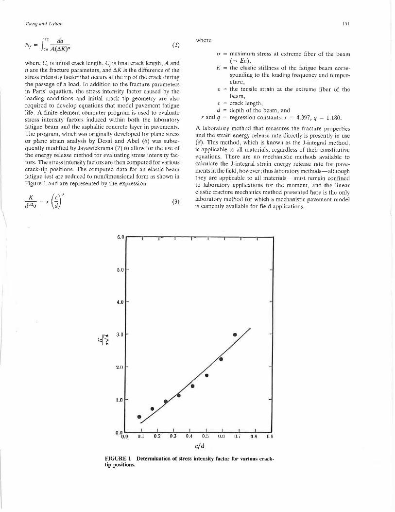
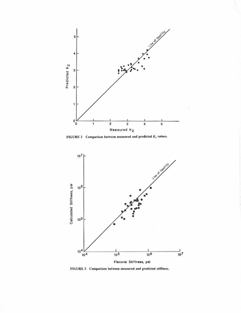
eters. Figure 2 shows the correspondence between the K 2
values obtained from the available fatigue data and the K2
values calculated by means of these two computer programs. As can be observed, the agreement between prediction and experiment is reasonable in general.
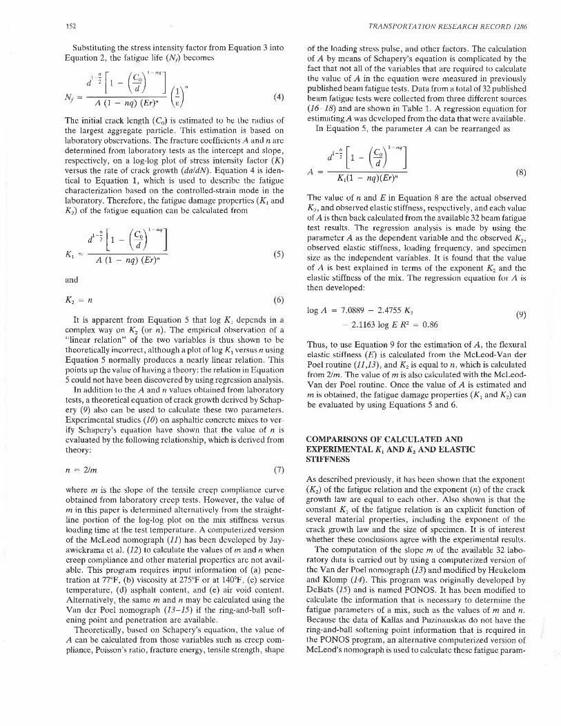
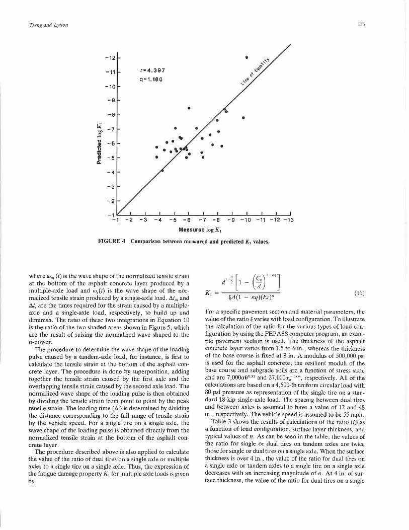
The moduli obtained from beam fatigue tests are referred to as the flexural elastic stiffness. It is necessary to know whether the stiffness calculated from the McLeod-Van der Poe! computer program will result in acceptable agreement with the measured flexural elastic stiffness. A comparison of the calculated elastic stiffness and those measured flexurfll elastic stiffnesses is shown in Figure 3. As seen in the figure, the measured and computed stiffness are in reasonable agreement.
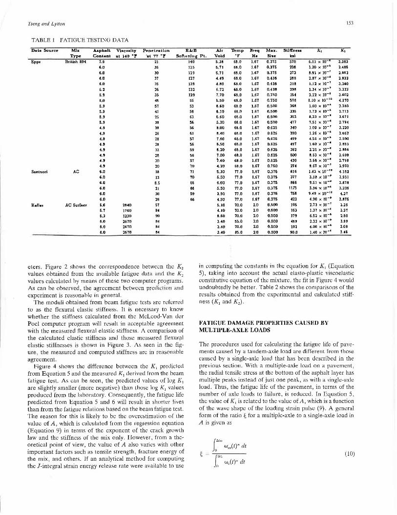
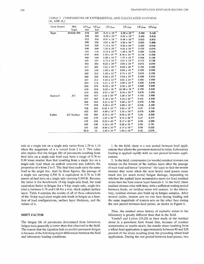
Figure 4 shows the difference between the K, predicted from Equation 5 and the measured K 1 derived from the beam fatigue test. As can be seen, the predicted values of log K 1
are slightly smaller (more negative) than those log K, values produced from the laboratory. Consequently, the fatigue life predicted from Equation 5 and 6 will result in shorter lives than from the fatigue relations based on the beam fatigue test. The reason for this is likely to be the overestimation of the value of A, which is calculated from the regression equation (Equation 9) in terms of the exponent of the crack growth law and the stiffness of the mix only. However, from a theoretical point of view, the value of A also varies with other important factors such as tensile strength, fracture energy of the mix, and others. If an analytical method for computing the !-integral strain energy release rate were available to use
140 125
129 127 129
1J2 129 55
SJ
58 6J 56 56
61 57 56 59
56 57 70
71 70 66 66
59
66
5.J8
5.71
5.71 4.49
4.80
6.7l 7.70 5.50 8.60 8.10 6.60 5.30 8.00
8.40 7.60 6.50
8.20 7.00 'i.60
4.20 5.JO
6.50
6.00 5.50 3.90
4.50
5.JO 4.10 8.60
3.40 3.40 3.40
68.0 68.0
68.0 68.0
68.0
68.0 68.0 68.0
68.0 68.0 68.0 68.0 68.0
68.0 68.0 68.0 68.0
68.0 68.0
68.0 77.0
77.0
77.0 77.0 77.0
77.0
70.0 70.0 70.0
55.0 70.0
85.0
1.67
1.67
J.67 J.67 1.67
J.67 J.67
1.67
1.67
O.J75
0.375
0.375 0.438 0.438
0.438 0.750 0.750
0.500 1.67 0.500 J.67 0.500
1.67 0.600 1.67 0.625 J.67 0.625 1.67 J.67 I.67
J.67 1.67 1.67
1.67
1.67
0.625 0.625 0.6l6 0.625 0.616 0.760
0.375 O.J75
1.67 0.375
1.67 0.375 J.67 0.376
1.67 0.375 2.0 0.500 2.0 0.600
2.0 0.500 2.0 0.500 2.0 0.500
l.O 0.500
570 ll8 l73
l88 318
298 164 576
368 3J5 303 477 HO 390 499 497
362 600 430
274
616
377 866
1175
758
411
195 163 179 469 192
90.0
6. JJ " 10-1
3.10 x 10-•
8.91 >< m-' l.87 x 10-•
J.ll >< m-'
1.34 x m-' 2.12 x m-•
I.JO >< m-•• 1.60 x m-•
3.JIJ 2.486 2.962
2.8l2 3.210
3.lll 3.101
4.170
2.360 1.13 x m-• 2.1n 8.23 x m-• 3.671
1.s1 x m-• 2.794 1.09 x m-' J.llO 1.26 x m-• 2.662 4.56 x m-• 1.60 x m-•
2.21 x m-• e.62 x m-• 3.68 x m-• !.67 x m-' 1.43 )( 10-•0
3.Je >< m-•
2.500 2.893 2.866
2.698 2.n8 2.970
4.18l J.931
9.5 I x m-• 3.678 3.36 x m-• 3.125 9.49 x rn- 11 4.n
4.90 x m-• 3.en
2.73 x m-' 3.25 1.37 )( 10-• 3.27
6.s2 x m-• 2.60 2.32 x 10-• 3.99 4.00 >< 10-• 3.08 1.40 x m-• J.41
in computing the constants in the equation for K 1 (Equation 5), taking into account the actual elasto-plastic viscoelastic constitutive equation of the mixture, the fit in Figure 4 would undoubtedly be better. Table 2 shows the comparisons of the results obtained from the experimental and calculated stiffness (K1 and K2 ).
FATIGUE DAMAGE PROPERTIES CAUSED BY MULTIPLE-AXLE LOADS
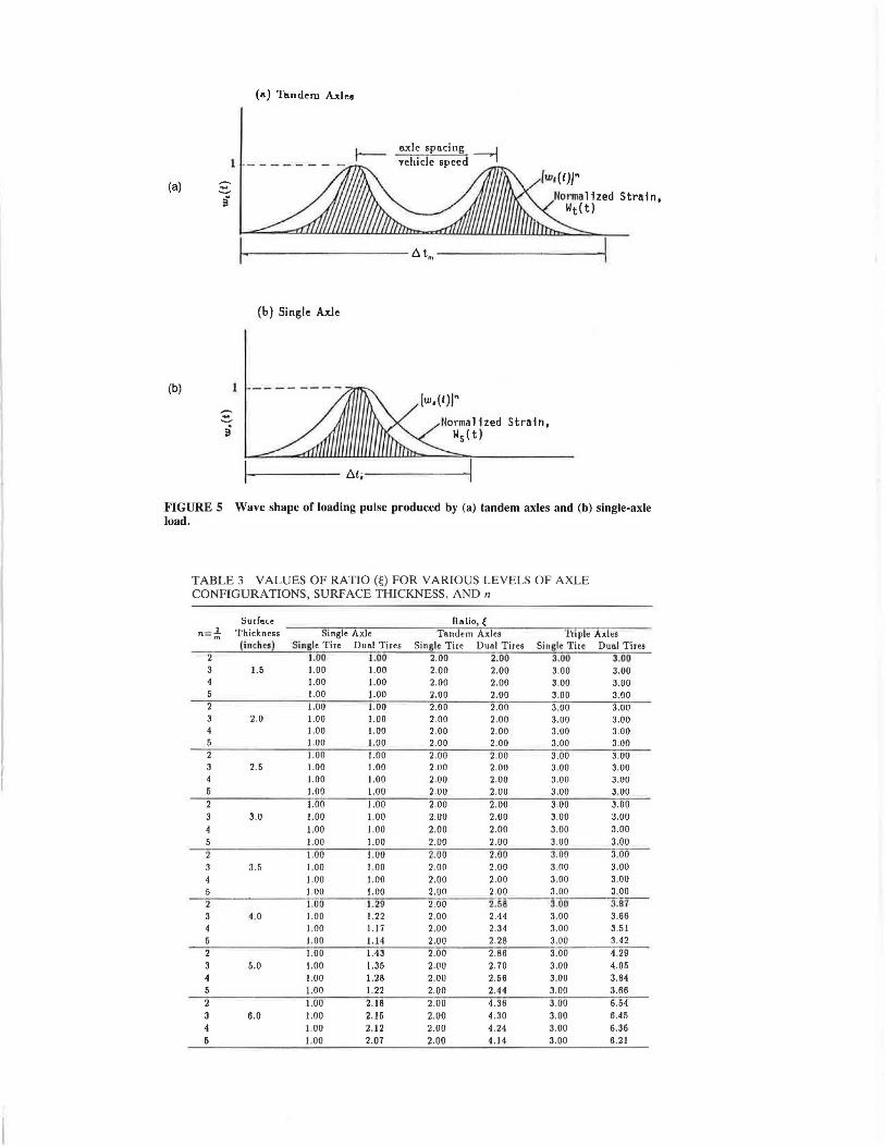
The procedures used for calculating the fatigue life of pavements caused by a tandem-axle load are different from those caused by a single-axle load that has been described in the previous section. With a multiple-axle load on a pavement, the radial tensile stress at the bottom of the asphalt layer has multiple peaks instead of just one peak, as with a single-axle load. Thus, the fatigue life of the pavement, in terms of the number of axle loads to failure, is reduced. In Equation 5, the value of K, is related to the value of A, which is a function of the wave shape of the loading strain pulse (9). A general form of the ratio ~ for a multiple-axle to a single-axle load in A is given as
{"''"' Jo wm(t)" dt
{"''' Jo w5 (t)" dt
(10)
4
C\I ~
"C 3
IP -(.)
"O IP .... a.. 2
Measured K2
FIGURE 2 Comparison between measured and predicted Ki values.
·u; 106 Cl.
.,; • UI •• IP c:
::::: :;:: Cl)
"O IP -ell :; (.) 105 iii l)
Flexural Stiffness, psi
FIGURE 3 Comparison between measured and predicted stiffness.
Tseng and Lytton 155
-12
-11 r-4.397
q-1.180 -10
-9
• -e
~ -7 • • bO • _g
' • 'g • QI -6 • • - • u 'ti • e -5 • • a.
-4
-3
-2
-2 -3 -4 -5 -6 -7 -e -9 -10 -11 -12 -13
Measured log [( 1
FIGURE 4 Comparison between measured and predicted K, values.
where wm (t) is the wave shape of the normalized tensile strain at the bottom of the asphalt concrete layer produced by a multiple-axle load and ws(t) is the wave shape of the normalized tensile strain produced by a single-axle load. l::i.tm and l::i.ts are the times required for the strain caused by a multipleaxle and a single-axle load, respectively, to build up and diminish. The ratio of these two integrations in Equation 10 is the ratio of the two shaded areas shown in Figure 5, which are the result of raising the normalized wave shaped to the n-power.
The procedure to determine the wave shape of the loading pulse caused by a tandem-axle load, for instance, is first to calculate the tensile strain at the bottom of the asphalt concrete layer. The procedure is done by superposition, adding together the tensile strain caused by the first axle and the overlapping tensile strain caused by the second axle load. The normalized wave shape of the loading pulse is then obtained by dividing the tensile strain from point to point by the peak tensile strain. The loading time (l::i.,) is determined by dividing the distance corresponding to the full range of tensile strain by the vehicle speed. For a single tire on a single axle, the wave shape of the loading pulse is obtained directly from the normalized tensile strain at the bottom of the asphalt concrete layer.
The procedure described above is also applied to calculate the value of the ratio of dual tires on a single axle or multiple axles to a single tire on a single axle. Thus, the expression of the fatigue damage property K 1 for multiple axle loads is given by
I-~ [ (Co)l-nq] d 2 1 - -d
(11) £,4(1 - nq)(Er)n
For a specific pavement section and material parameters, the value of the ratio~ varies with load configuration. To illustrate the calculation of the ratio for the various types of load configuration by using the FEP ASS computer program, an example pavement section is used. The thickness of the asphalt concrete layer varies from 1.5 to 6 in., whereas the thickness of the base course is fixed at 8 in. A modulus of 500,000 psi is used for the asphalt concrete; the resilient moduli of the base course and subgrade soils are a function of stress state and are 7 ,000rr0°·35 and 27 ,OOOu .f 1.o6
, respectively. All of the calculations are based on a 4,500-lb uniform circular load with 80 psi pressure as representation of the single tire on a standard 18-kip single-axle load. The spacing between dual tires and between axles is assumed to have a value of 12 and 48 in., respectively. The vehicle speed is assumed to be 55 mph.
Table 3 shows the results of calculations of the ratio (~) as a function of load configuration, surface layer thickness, and typical values of n. As can be seen in the table, the values of the ratio for single or dual tires on tandem axles are twice those for single or dual tires on a single axle. When the surface thickness is over 4 in., the value of the ratio for dual tires on a single axle or tandem axles to a single tire on a single axle decreases with an increasing magnitude of n. At 4 in. of surface thickness, the value of the ratio for dual tires on a single
156 TRANSPORTATION RESEARCH RECORD 1286
TABLE 2 COMPARISONS OF EXPERIMENTAL AND CALCULATED STIFFNESS (K1 AND K 2 )
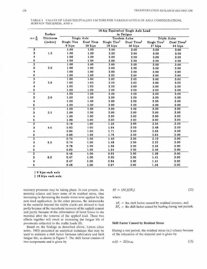
axle to a single tire on a single axle varies from 1.29 to 1.14 when the magnitude of n is varied from 2 to 5. This value also implies that the fatigue life of pavements resulting from dual tires on a single-axle load may have a range of 0. 78 to 0.88 times smaller than that resulting from a single tire on a single-axle load when an asphalt concrete mix exhibits the properties of n from 2 to 5. The dual tires each carry the same load as the single tire. And by these figures, the passage of a single tire carrying 4,500 lb is equivalent to 0.78 to 0.88 passes of dual tires on a single axle carrying 9,000 lb. Because the latter is the benchmark 18-kip single-axle load, the load equivalent factor in fatigue for a 9-kip single-axle, single-tire load is between 0. 78 and 0.88 for a 4-in.-thick asphalt surface layer. Table 4 contains the results of all of these calculations of the 18-kip equivalent single-axle loads in fatigue as a function of load configurations, surface layer thickness, and the values of n.
SHIFT FACTOR
The fatigue life of pavements determined from laboratory fatigue tests generally is lower than that observed in the field. The reason that the equation fails to predict pavement fatigue is because of the following major differences between the field and laboratory loading conditions:
(Kt) .. , (KiJcar (/C2)eep (1<2) .. 1
6. lJ x L0 - 8 3.39 x 10- e 3.383 3.143 3.20 x 10- 5 8.21 x 10- 1 2.485 2.810 8.91 x 10- 1 6.44 x 10⁻⁸ 2.962 2.910 2.81 x 10- 9 4.29 X 10⁻⁷ 2.832 2.980 u2 x 10- 1 4.52 X 10- 7 3.260 3.010 t.34 x 10- 1 4.61 x iu- 0 3.222 2.870 2.12 x 10⁻⁹ 1.30 x lo- 8 3.602 3.030 1.lOxlO-ID 8.16 x 10- 1• 4.170 4.220 l.60 x IU- 4 l. 77 x 10- 9 2.350 3.190 1. 73 x 10- 9 4.0l x io- 8 2.713 3.120 8.23 x 10- 9 1:62 x lu- 8 3.671 3.470 7.51 x 10- 9 8.59 x lo- 8 2.i94 3.260 1.09 X 10- 7 8.80 x 10- 8 3.220 2.960 1.26 x iu- 1 6.7lxlU- 7 2.652 3.190
4.56 x 10- 1 5.53 x 10⁻⁹ 2.500 3.010
l.60 x I 0- 9 2.01 x 10- 0 2.893 2.960 2.21 x 10- 9 2.G8 x 10-8 2.850 3.060
8.52. x 10- 9 2.35 x lo- 0 2.698 2.990
3.58 x 10- 9 62.48 x 10⁻⁸ 2.798 3.030 9.67 X 10- 7 3.34 x 10- 9 2.970 3.354 l.43 X 10-ID 1.20 X 10-B 4.182 3.988
3.18 x 10- 9 4.13 x 10- 9 3.931 4.018 9.51 x 10- 9 2.56 x 10- 9 3.678 3.785 3.36 x 10- 9 2.60x 10- 1 3.225 3.369
9.49 x 10- 11 3.83 x I o-e 4.27 3.746 4.9o x 10- 9 1.46 x 10⁻⁸ 3.876 3.266 2.73 x 10- 7 6.63 X 10-B 3.25 3.368 1.37 x 10-G 2.71 x 10-e 3.27 3.177
6.52 x 10- 1 8.17 x 10- 1 2.50 2.960 2.32 x 10- 9 6.26 x 10- 9 3.99 3. 731 4.00 x 10- 9 3.77 X 10- 7 3.08 3.332 l.40 x 10- 9 LOO x 10- 9 3.45 3.070
1. In the field, there is a rest period between load applications that allows the pavement material to relax. Laboratory loading is applied rapidly with no rest pt:riml between applications.
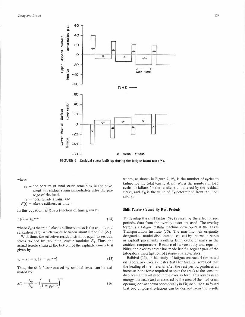
2. In the field, compressive (or tensile) residual stresses can remain on the bottom of the surface layer after the passage of each load and hence "prestress" the layer so that the tensile stresses that occur when the next heavy load passes cause much less (or much more) fatigue damage , depending on whether the asphalt layer accumulates more (or less) residual stress than the base course layer beneath it. In the field, these residual stresses relax with time; with a sufficient waiting period between loads, no residual stress will remain. In the laboratory, residual stresses also build up in fatigue samples. After several cycles, tension acts on one face during loading and the same magnitude of tension acts on the other face during the rest period between load pulses, as shown in Figure 6.
Thus, the residual stress history of asphaltic mixes in the laboratory is greatly different than that in the field .
Yandell and Lytton (19,20) in their study of the residual stress in a pavement have found that, because of residual compressive or tensile strain, the tensile stress resulting from a wheel load application is approximately between 80 and 120 percent of the strain resulting from the preceding wheel load application. During the rest period between load passes, two
recovery processes may be taking place. In one process, the material relaxes and loses some of its residual stress, thus increasing or decreasing the tensile stress level applied by the next load application. In the other process, the microcracks in the material beyond the visible cracks are allowed to heal partly because of the viscoelastic recovery of the asphalt cement and partly because of the reformation of bond forces in the material after the removal of the applied load. These two effects together will result in increasing the fatigue life of pavements subjected to the traffic loads (8).
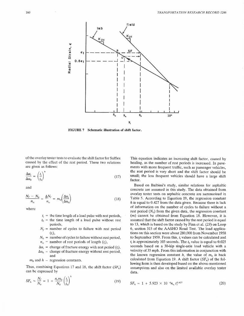
Based on the findings as described above, Lytton (class notes, 1983) presented an analytical technique that may be used to estimate a shift factor between laboratory and field fatigue life, as shown in Figure 7. The shift factor consists of two components and is given by
SF, = the shift factor caused by residual stresses, and SFh = the shift factor caused by healing during rest periods.
Shift Factor Caused by Residual Stress
During a rest period, the residual stress (a,) relaxes because of the relaxation of the material and is given by
a,(t) = E(t)E,p0 (13)
Tseng and Lytton 159
60 -"' ci.
c: 40 .. 0 u 'iii
- -.E "' .... ..
:::> a. 20 (/) E 0
c u
-- ,._. -1-e- -e- -e- -G-
.c 0 0.
"' <(
-&- ~ -e-
.... -20 .. B: c:
:::> 0 ·;;; -40 c: wait time .
.!!
-60 -TIME -
60
c: 40 0 ·;;;
"' .. .. u .... 0 Q. 20 ~ E
0 u
c 0 .c Q.
"' <( -20 .... .. c: 3 0 0 ·;;;
-40 _J c .!!
-60 + mean stress
FIGURE 6 Residual stress built up during the fatigue beam test (15).
where
Po the percent of total strain remaining in the pavement as residual strain immediately after the passage of the load,
E = total tensile strain, and E(t) elastic stiffness at time t.
In this equation, E(t) is a function of time given by
(14)
where £ 0 is the initial elastic stiffness and mis the exponential relaxation rate, which varies between about 0.2 to 0.8 (21) .
With time, the effective residual strain is equal to residual stress divided by the initial elastic modulus E0 • Thus, the actual tensile strain at the bottom of the asphaltic concrete is given by
(15)
Thus, the shift factor caused by residual stress can be estimated by
(16)
where, as shown in Figure 7, N10 is the number of cycles to failure for the total tensile strain, N1c is the number of load cycles to failure for the tensile strain altered by the residual stress, and K21 is the value of K2 determined from the laboratory.
Shift Factor Caused By Rest Periods
To develop the shift factor (SFh) caused by the effect of rest periods, data from the overlay tester are used. The overlay tester is a fatigue testing machine developed at the Texas Transportation Institute (JO). The machine was originally designed to model displacement caused by thermal stresses in asphalt pavements resulting from cyclic changes in the ambient temperature. Because of its versatility and repeatability, the overlay tester has made itself a regular part of the laboratory investigation of fatigue characteristics.
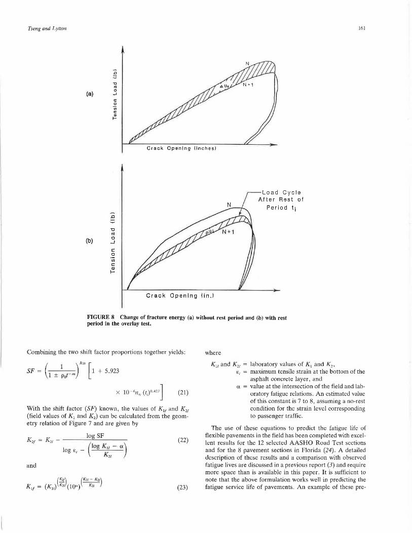
Balbissi (22), in his study of fatigue characteristics based on laboratory overlay tester tests for Sulflex, revealed that the healing of the material after the rest period produces an increase in the force required to open the crack to the constant displacement level used in the overlay test. This results in an energy increase (~u,.) as assessed by the area of the load-crack opening loop as shown conceptually in Figure 8. He also found that two empirical relations can be derived from the results
160 TRANSPORTATION RESEARCH RECORD 1286
Ill
c al Et ...
I c -CJ)
---1 _I iii
0.8Et I I "C I a!
I a: I I I I I I I I
I I I I
I N,. N,,, N.
N,
FIGURE 7 Schematic illustration of shift factor.
of the overlay tester tests to evaluate the shift factor for Sulflex caused by the effect of the rest period. These two relations are given as follows:
!::~ = (~r (17)
and
where
(18)
t; = the time length of a load pulse with rest periods, t0 = the time length of a load pulse without rest
periods , N1 = number of cycles to failure with rest period
(t,), N 0 = number of cycles to failure without rest period, n,; = number of rest periods of length (t;),
l::.u; = change of fracture energy with rest period (t;), l::.u0 = change of fracture energy without rest period,
and m0 and h = regression constants.
Thus, combining Equations 17 and 18, the shift factor (SFh) can be expressed by
SFh = Nr = 1 + n,mo (!i.)1r No No to
(19)
This equation indicates an increasing shift factor, caused by healing, as the number of rest periods is increased. In pavements with more frequent traffic, such as passenger vehicles, the rest period is very short and the shift factor should be small; the less frequent vehicles should have a large shift factor.
Based on Balbissi's study, similar relations for asphaltic concrete are assumed in this study. The data obtained from overlay tester tests on asphaltic concrete are summarized in Table 5. According to Equation 19, the regression constant h is equal to 0.427 from the data given. Because there is lack of information on the number of cycles to failure without a rest period (N0 ) from the given data, the regression constant (m) cannot be obtained from Equation 18. However, it is assumed that the shift factor caused by the rest period is equal to 13, which is based on the study by Finn et al. (23) on Loop 6, section 315 of the AASHO Road Test. The load applications on this section were about 280,000 from November 1958 to September 1959. From this, t; values can be calculated and t; is approximately 103 seconds. The t0 value is equal to 0.025 seconds based on a 30-kip single-axle load vehicle with a velocity of 35 mph. From this information in conjunction with the known regression constant h, the value of m0 is back calculated from Equation 19. A shift factor (SFh) of the following form is then developed based on the above-mentioned assumptions and also on the limited available overlay tester data.
(20)
Tseng and Lytton
(a)
.!J
"tJ
'" 0 -I
c: 0
"' c: ~
161
Crack Ope n ing llnches)
(b)
"tJ rd 0 .J
c: 0 (I]
c: QI I-
Load Cycle After Rest of
Period ti
Crack Opening Un . )
FIGURE 8 Change of fracture energy (a) without rest period and (b) with rest period in the overlay test.
Combining the two shift factor proportions together yields:
SF = (l l )K" [1 + 5.923 ± Pol- "'
x 10-6n,, (t;)o421] (21)
With the shift factor (SF) known, the values of Klf and K 21 (field values of K 1 and K 2 ) can be calculated from the geometry relation of Figure 7 and are given by
log SF Kzt = Kz1 - ------=-----
- (log K ,1 - a) loge, Ku
and
(22)
(23)
where
K11 and K21 = laboratory values of K1 and K2 ,
e, = maximum tensile strain at the bottom of the asphalt concrete layer, and
ex = value at the intersection of the field and laboratory fatigue relations. An estimated value of this constant is 7 to 8, assuming a no-rest condition for the strain level corresponding to passenger traffic.
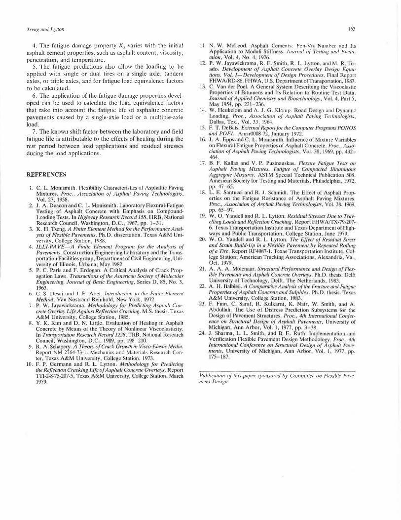
The use of these equations to predict the fatigue life of flexible pavements in the field has been completed with excellent results for the 12 selected AASHO Road Test sections and for the 8 pavement sections in Florida (24). A detailed description of these results and a comparison with observed fatigue lives are discussed in a previous report (J) and require more space than is available in this paper. It is sufficient to note that the above formulation works well in predicting the fatigue service life of pavements. An example of these pre-
162
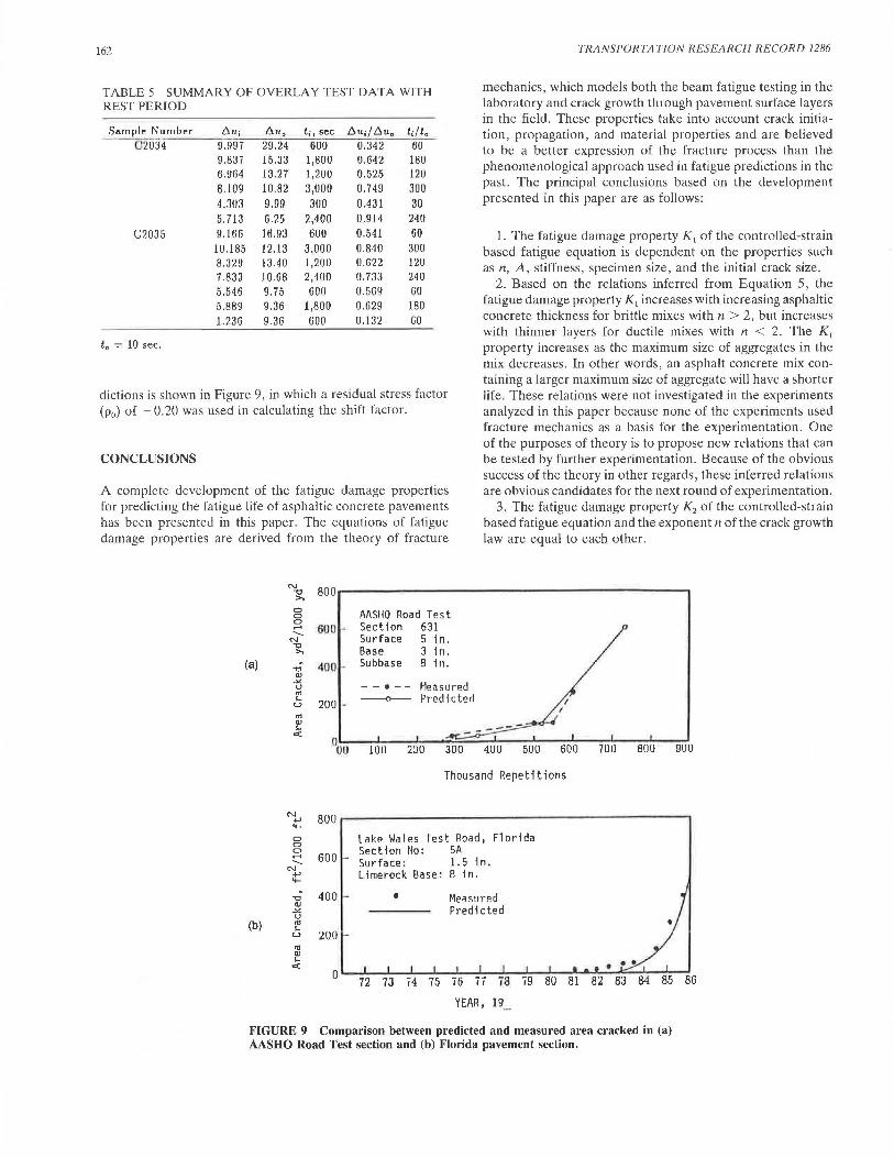
TABLE 5 SUMMARY OF OVERLAY TEST DATA WITH REST PERIOD
dictions is shown in Figure 9, in which a residual stress factor (p0) of - 0.20 was used in calculating the shift factor.
CONCLUSIONS
A complete development of the fatigue damage properties for predicting the fatigue life of asphaltic concrete pavements has been presented in this paper. The equations of fatigue damage properties are derived from the theory of fracture
N 800 " >.
TRANSPORTATION RESEARCH RECORD 1286
mechanics, which models both the beam fatigue testing in the laboratory and crack growth through pavement surface layers in the field. These properties take into account crack initiation, propagation, and material properties and are believed to be a better expression of the fracture process than the phenomenological approach used in fatigue predictions in the past. The principal conclusions based on the development presented in this paper are as follows:
1. The fatigue damage property K 1 of the controlled-strain based fatigue equation is dependent on the properties such as n, A, stiffness, specimen size, and the initial crack size.
2. Based on the relations inferred from Equation 5, the fatigue damage property K 1 increases with increasing asphaltic concrete thickness for brittle mixes with n > 2, but increases with thinner layers for ductile mixes with n < 2. The K 1
property increases as the maximum size of aggregates in the mix decreases. In other words, an asphalt concrete mix containing a larger maximum size of aggregate will have a shorter life. These relations were not investigated in the experiments analyzed in this paper because none of the experiments used fracture mechanics as a basis for the experimentation. One of the purposes of theory is to propose new relations that can be tested by further experimentation. Because of the obvious success of the theory in other regards, these inferred relations are obvious candidates for the next round of experimentation.
3. The fatigue damage property K 2 of the controlled-strain based fatigue equation and the exponent n of the crack growth law are equal to each other.
CJ AASHO Road Test CJ CJ ...... 600 ---..
N
" >.
(a) " 400
QJ ->< u
"' .... 200 -LJ
"' QJ .... c:(
0uu
N 800 .µ .... CJ CJ Cl ...... 600 --..
N .µ .... .,; 400 QJ
->< u (b) "' ....
200 t..J
"' QJ .... c:(
0
Section 631 Surface 5 in. Base 3 in. Subbase B in.
--·-- Measured ---0-- Predicted
lOU 2UU 300 400 50U
I I
600
Thousand Repetitions
Lake Wales Test Road, Florida Section No: SA Surface: 1. 5 in. Limerock Base: B in.
• Measured Predicted
72 73 i4 75 76 jj i8 ;g 80 Bl
YEAR, 19_
7UO BOU
82 83 84 85
FIGURE 9 Comparison between predicted and measured area cracked in (a) AASHO Road Test section and (b) Florida pavement section.
900
86
Tseng and Ly/Ion
4. The fatigue damage property K 2 varies with the initial asphalt cement propertie , such as asphalt content, viscosity, penetrati.on and temperature.
5. The fatigue predictions also allow the loading to be applied with single or dual tires on a single axle , tandem axles, or triple axles, and for fatigue load equivalence factors to be calculated.
6. The application of the fatigue damage properties developed can be used to calculate the load equivalence factors that take into account the fatigue life of asphallic concrete pavements caused by a single-axle load or a multiple-axle load.
7. The known hift factor between th laborat ry and fie ld fatigue life is attributable to the effect · of hea ling during the rest period between load application and residual st res. e. during the load applications.
REFERENCES
1. . L. Monismith. Flexibility Characteristics of Asphaltic Paving Mixtures. Proc., Associmion of A phalt Paving Tecli11ologis1s, Vol. 27 1958.
2. J . A. Deacon and . L. M,onismith. Laboratory F lexural-Fatigue Testing of Asphal t Concrcce wich Empha is n ompoundLoading Tc t. . In Highway Research Record 158. HRB , National Research C unci l, Wahington , D .. , 1967, pp. 1-31.
3. K. H. Tseng. A Fi11i1e Elem em Me1hotl for tlrl' Per[ or111a11ce Analysis of Flexible Pavem 111s. Ph .D. di crtati n. Texa A&M University, College Station, 1988.
4. /LU-PA \IE- A Finite Eleme/11 Program for tire A1111lysi of Paveme11t.f. on truccion Engi neeri ng Labon1tory and 1hc Trn nsp rtation Facililie! group , D1;:partment of Civil Engi neering University of Hlinois, Urbana, May 1982.
5. P. C. Puri. nnd F. Erdogan. A ricica l Analy •is of rack Propagation Law . Tra11sactio11S of tlie American Society of Molectilnr E11gimwri11g, Joumal of Bnsic E11gi11eeri11g , erics D . 85, No. 3, 1963.
6. C. S. Desai and J . F . Abel. lntroduclion 10 the Finite Element Method. Van Nostrand Rein.hold , New York, 1972.
7. P. W. Jayawickrama. Me1hodology .for Pretlic1i11g I\ phalt Concre1e 011erlay Life Against Ref/1$ 1io11 Crncking. M ... thesis. Texas A •M University, College Station . 1985.
8. Y. K. Kim and D. N, LiHlc. Evaluacicrn of Healing in A ·pln1lt Concrete by Mea ns of the Theory f Nonlinear iscoclas1ici1y . In Tramporwrion Research Record 1228, T RB , National R carch Council. Washingt n, D .. , 1989 .. pp. 198-210.
9. R . A. Schnpery. A Theory of Crack Growth in Visco-Elastic Media. Report NM 2764-73-1. Mechanics and Materials Research Center, Texa A&M UniveT'ity , College Su11 ion, 1973.
10. F. P. Germann and R. L. Lyllon . Methodology for J'ratllc1i11g rile Ref/euion mcki11g Life of Asphal1 Com·r11te Overlays. Repon ·m-2-8-75-207-5, Tcxa A&M Univcrsicy, a llege Stati n, March "1979.
163
11. N. W. Mcleod. Asphalt cmcnts : Pen-Vi Number and Its Applica1ion to Moduli Stiffnes . Journal of Tes1ing and Evaluwio11 , Vol. 4. No. 4. 1976.
12. P. W. Jayawickrama, R. E. milh . R. L. Lycton. and M. R. Tirado. Dev •/opme111 of A.l'phn// om:retc Overlay Design £qua-1io11s. Vol. l- Developme111 of Design Procedures. Final Rcporl FHWAIRD-86. FHWA, U.S. Dcpartmcnt ofTranspormtion, 19 7.
13. . Van dcr Poel. A General y tem Des ·ribing the Viscocla tic Propercics of Bitumens and lts Relation 10 Ro111 inc es t D<lla. Jo11m11/ ·of Applied Cltemislr)' and 8io1ec/111ology. V I. 4, Parl 5, tvhy 1954. pp. 221- 236.
14. W. Hcukelom and A. J. G. Klomp. Road D~ ign and Dynamic Loading. Proc .. Association of Asplwll Pm•ing Tech11ologi ts, Dallas, Tex .. Vol. 33, 1964 .
15. F. T. 'DeBat . E.x1ema/ Reporl for the ompwer Programs PONO <md POEt . AmsrOOO -72, Jnnuary 1972.
16. J. A. Ep1 sand . L. Monismith . Influence of Mixture Variables on Flexural Fatigu Properties of Asphalt Concrete. Proc., Assoda1io11 of Asvlwl1 Pa11i11g Tec/1110/ogist.v, Vl~I. 3 , 1969, pp. 432-4 4.
17. B. F. Kallas and V. P. Puzinauskas. Flexure Fa1igue Te. ·1 011 Aspha/r Pm•i11g Mixttll'es. Fmigm.> of Compac1ed 8it11111i11()11 Aggregllle Mixiures. A TM pecial Technical Publication 50 . American Society fo r Testing and Materials. Philadelphia, 1972, pp. 47-65.
18. L. E. Snntucci and R. J. Schmidt. T he Ef[ c1 of Asphah Propen ies on 1hc Facigue Resista nce f Asphah Paving Mixtures. Proc., Assocla1io11 of Asphalt Paving Tech11ologisrs Vol. 38, 1969, pp. 65-97.
19. W. 0 . Yandell and R. L. Lynon . Residual Srresses Due to Tra1•elli11g Lomts and l?eflection r11cki11g. Report FI I W ArrX-79-207-6. Texn Transporcaiion lns1itutc and Texa DepHrtmcnl of Highways and Public Tran ·porrntion. ollcge Station, June 1979.
20. W. 0. Yandell and R . L. Lyuon. Tlie Effect of R1:sid11fll Stress and train 811i/1l-Up in a flexible Pavemem b Repemed Rolling of fl Tire. Report RF40 7-l. Texas Transportation l11s1i1utc, a llege Station; American Trucking Ass ciations, Alexandria. Va ., Oct. 1979.
2 1. A. A. A. Molennar. 1rnc1w·n/ Pe1fomw11ce and D ig11 of Flexible. Paveme111s mul Asplra/r Concrete Overlay~-. Ph.D. thesi . Delft University of Technology, Delft , he Netherlands. 1983.
22. A. H. Ba Ibis i. A Comparmivc A11aly is of 1/re Frnc111re a11d Fu1ig11e Properries of Asphalt 011cre1e and S11lpl1/ex. Ph.D. ch is. Tcxa A&M University. ollcgc Station, 1983 .
23. F. Finn , . Sara(, R. Kulkarni , K. Nair, W. mith , :111d A. Abdullah. The Use of Distress Predic1io11 ubsy tern · for 1hc Design of Pavement truclure" Proc., 4rh l111emmio11al Co11fere11ce 011 Structural D ig11 of I\ pha/1 Pavc111e111s, Univer, i1y f Michiga n, Ann Arbor, Vol. l. 1977, pp. -38.
24. J . Sharma, L. L. Smith, and B. E. Ruth. Imp! men1u1ion and Verification Flex ible Pavement Design Methodology. Proc., 4th /111ematio11al onfer«flfil! 0 11 1ruc111ra/ De ig11 of A plw/1 f'a11eme11ts, Univer ity of Michigan, Ann Arb r, ol. I, 1977. pp. 175-187.
Publication of this paper sponsored by Committee on Flexible Pavement Design.