Fault Detection for Industrial Processes - Hindawi...

Hindawi Publishing CorporationMathematical Problems in EngineeringVolume 2012, Article ID 757828, 18 pagesdoi:10.1155/2012/757828

Research ArticleFault Detection for Industrial Processes

Yingwei Zhang, Lingjun Zhang, and Hailong Zhang

State Laboratory of Synthesis Automation of Process Industry, Northeastern University,Liaoning, Shenyang 110004, China

Correspondence should be addressed to Yingwei Zhang, [email protected]

Received 23 August 2012; Accepted 15 November 2012

Academic Editor: Huaguang Zhang

Copyright q 2012 Yingwei Zhang et al. This is an open access article distributed under theCreative Commons Attribution License, which permits unrestricted use, distribution, andreproduction in any medium, provided the original work is properly cited.

A new fault-relevant KPCA algorithm is proposed. Then the fault detection approach is proposedbased on the fault-relevant KPCA algorithm. The proposed method further decomposes both theKPCA principal space and residual space into two subspaces. Comparedwith traditional statisticaltechniques, the fault subspace is separated based on the fault-relevant influence. This methodcan find fault-relevant principal directions and principal components of systematic subspaceand residual subspace for process monitoring. The proposed monitoring approach is applied toTennessee Eastman process and penicillin fermentation process. The simulation results show theeffectiveness of the proposed method.

1. Introduction

Process monitoring and fault diagnosis are important for the safety and reliability ofindustrial processes [1–12]. As a data-driven process monitoring methodology, multivariatestatistical analysis techniques, such as principal component analysis (PCA) and partial leastsquares (PLS), have been used widely for detection and diagnosis of abnormal operatingsituations in many industrial processes in the last few decades [5, 13–16]. The majoradvantage of these methods is ability to handle larger number of highly correlated variablesand reduce the high-dimensional process measurement into a low-dimensional latent space.The monitoring based on these methods is straightforward.

PCA is one of the most widely used linear techniques for transforming data into anew space. It divides data information into the significant patterns, such as linear tendenciesor directions in model subspace, and the uncertainties, such as noises or outliers located inresidual subspace. T2 statistic and SPE statistic, represented by Mahalanobis and Euclidiandistances, are used to elucidate the pattern variations in the model and residual subspaces,respectively [17–19]. PLS decomposition methods are used similar to PCA for process

2 Mathematical Problems in Engineering

monitoring and are more effective in supervising the variations in the process variablesthat are more influential on quality variables [20–22]. T2 statistic and SPE statistic are alsoemployed in the PLS monitoring system. These methods develop a normal operating modelwith the normal data gathered from the normal process and define the normal operationregions. The new process behaviors can thus be compared with the predefined ones by themonitoring system to ensure whether they remain normal or not. When the process movesout of the normal operation regions, it is concluded that an “unusual and faulty” changein the process behaviors has occurred. Nowadays, many extensions of the conventionalPCA/PLS algorithms have been reported [15, 23–31]. Recently, Li et al. proposed a totalprojection to latent structure (T-PLS) and discussed the policy of process monitoring andfault diagnosis based on the new structure [32, 33]. They analyzed the problem faced inconventional PLS based process monitoring policy which only divides the measured variablespace into two subspaces and uses two monitoring statistics for PLS scores and residuals,respectively. They indicated that the output-irrelevant variations are also included by PLSscores and PLS residuals do not necessarily cover only small X-variations. The proposedT-PLS algorithm further decomposed the PLS systematic subspace to separate the output-orthogonal part from the output-correlated part, and the PLS residual subspace to separatelarge variations from noises. T-PLS based monitoring system was then developed based onthe four-process subspace.

KPCA is one nonlinear version of PCA. It can efficiently compute PCs in a high-dimensional feature space using nonlinear kernel functions. The core idea of KPCA is to firstmap the data space into a feature space using a nonlinear mapping and then carry out thePCA operation in the feature space. KPCA divides the data into a systematic subspace anda residual subspace and uses T2 statistic and SPE statistic to monitor these two subspaces,respectively [13, 15, 16, 34].

In this paper, to improve the KPCA model, a fault-relevant KPCA algorithm isproposed and the approach of process monitoring based on the new fault-relevant KPCAalgorithm is proposed for fault detection. The proposed method further decomposes both theKPCA principal space and residual space into two subspaces by checking the influences byprocess disturbances. The basic objective for further subspace decomposition is to separatethe part which is influenced greatly by the fault from the part that is not clearly fault-relevant,that is, to find the fault-relevant directions and fault-relevant principal components. Then anew monitoring method is proposed based on the fault-relevant directions. Compared withtraditional statistical techniques, the fault subspace is separated based on the fault-relevantinfluence.

The remaining sections of this paper are organized as follows. Section 2 revisits theKPCA model and then presents the fault-relevant KPCA algorithm. Section 3 introducesthe on-line monitoring method of fault-relevant KPCA. Model development and on-linemonitoring are proposed in Section 3. In Section 4, the simulation results are given to illustratethe effectiveness of the new method. At last the conclusions are drawn in Section 5.

2. Algorithm of Fault-Relevant KPCA

For the traditional PCA algorithm, some faults may not influence all the principal directions;that is, to a given fault, some principal directions are not relevant. KPCA algorithm is themethod for nonlinear data extended from PCA algorithm, so it has the same characteristicsmentioned above [35]. The proposed fault-relevant KPCA algorithm finds the principal

Mathematical Problems in Engineering 3

directions which are relevant to, or affected by the disturbances and then measures thechanges of the variation along these principal directions. Therefore the proposed algorithmhas higher sensitivity and accuracy for process monitoring and it can detect the faults faster.

The purpose of the proposed algorithm is to get the fault-relevant principal directionsin the systematic subspace and those of the residual subspace. With the obtained fault-relevant principal directions and a new set of data, the scores of new data can be gotten.Therefore, the T2 statistic and SPE statistic can be further calculated to monitor the process.

In KPCA, the training samples x1, x2, . . . , xN ∈ RM gotten from normal process aremapped into feature space using nonlinear mapping:Φ : RM → F. The covariance matrix inthe feature space F can be calculated as follows:

CΦ =1N

N∑

j=1

Φ(xj)Φ(xj)T, (2.1)

where it is assumed that∑N

k=1 Φ(xk) = 0, and Φ(·) is a nonlinear mapping function thatprojects the input vectors from the input space to F. Principal components in F can beobtained by finding eigenvectors of CΦ, which is straightforward to the PCA procedure ininput space, using the equation as follows:

λp = CΦp, (2.2)

where λ denotes eigenvalues and p denotes eigenvectors of covariance matrix CΦ.For λ/= 0, solution p (eigenvector) can be regarded as a linear combination of

Φ(x1),Φ(x2), . . . ,Φ(xN), that is, p =∑N

j=1 αjΦ(xj).Using kernel trickKij = 〈Φ(xi) ·Φ(xj)〉, the eigenvalue problem can be expressed as a

simplified form as follows:

λα =(

1N

)Kα, (2.3)

where α = [α1α2 · · ·αN]T and K ∈ RN×N are a gram matrix which is composed of Kij .Then, the calculation is equivalent to resolving the eigen problem of (2.3). To satisfy the

assumption∑N

k=1 Φ(xk) = 0,K must be mean-centered before the calculation. The centeredgram matrix K can be easily obtained by K = K − KE − EK + EKE, where each element ofE is equal to 1/N and E ∈ RN×N . Also, the coefficient α should be normalized to satisfy‖α‖2 = (1/N)λ, which corresponds to the normality constraint, ‖p‖2 = 1 of eigenvector.

The scores T of vector X are then extracted by projecting Φ(x) onto eigenvectors p inF and the number of scores is N. As some principles, R scores are selected to be principalcomponents, and R corresponding directions of p are gotten at the same time [36, 37]. Rdirections selected from p span the systematic subspace and the remaining N-R directionsspan the residual subspace. The PCs of X is

T = [t1t2 · · · tR],

tk = 〈pk,Φ(x)〉 =N∑

i=1

αki 〈Φ(xi),Φ(x)〉 = Kαk,

(2.4)

where k = 1, . . . , R, and R is the number of principal components.


Now PCs of training data are gotten the PCs that are relevant to faults will be foundnext as follows.

First, a fault process spaceΦf(x) is separated into a systematic subspace and a residualsubspace following the separation rule of the process space Φ(x). One data set Xf ∈ RL×M

collected from a fault case is projected into F with the same mapping function Φ(·) to getΦf(x)

Tf =[tf,1tf,2 · · · tf,R

],

tf,k =⟨pk,Φf(xi)

⟩

=N∑

i=1

aki

⟨Φf(xi),Φ(xi)

⟩

= Kfαk,

(2.5)

where Kf,ij = (Φf(xi) ·Φ(xj)), Kf = Kf − EL×NK −KfE + EL×NKE, and

EL×N =1N

⎡⎢⎣

1 · · · 1...

. . ....

1 · · · 1

⎤⎥⎦ ∈ RL×N. (2.6)

Tf spans the systematic subspace of Φf(x).Then, the fault-relevant PCs of fault data Φf(x) can be gotten via

Tf,r =⟨Pr ,Φf(x)

⟩,

Pr =[pr,1pr,2 · · · pr,l

],

pr,l =N∑

j=1

αljΦ

(xj), l = 1, . . . , Rf,r .

(2.7)

From (2.7), (2.8) can be obtained as follows:

tlf,r = Kfαl, l = 1, . . . , Rf,r , (2.8)

where Rf,r = rank(Tf), and the subscript r denotes fault relevant.And the fault-relevant PCs of normal data Φ(x) can be calculated with the same

principle:

Tr = 〈Pr ,Φ(x)〉,

tlr = Kαl, l = 1, . . . , Rf,r .(2.9)


In this way, some largest fault-relevant directions of normal data and fault data arerevealed, respectively. Define the ratio of the fault-relevant PC variances between fault caseand normal case as follows:

Ratioi =var

(Tf,r(:, i)

)

var(Tr(:, i)), i = 1, 2, . . . , Rf,r , (2.10)

where var(·) denotes the variance of PCs and Tf,r(:, i) denotes the ith column vector in matrixTf,r as well as Tr(:, i).

The largest value of Ratioi denotes the direction along which there are the largestchanges of process variation from normal status to fault case. If the Ratioi index is smallerthan 1, it means that the concerned variations in the fault status are smaller than those innormal case. Keep the directions with values of larger than 1 which are the fault-relevantdirections with increased variations. The number of retained principal directions is Rp. TheRp fault-relevant principal directions compose Pp and the remaining R-Rp directions of Pr ,which are fault irrelevant, compose Po. Tp are the fault-relevant PCs of normal data with Rp

components and To are the fault-irrelevant PCs, with R-Rp components.The pk =

∑Nj=1 α

kj Φ(xj), k = 1, . . . , R span the systematic subspace and the pk =

∑Nj=1 α

kj Φ(xj), k = R + 1, . . . ,N span the residual subspace. Define the column number of

principal directions in residual subspace are R∗, R∗ = N − R and define P∗ as follows:

P∗ =[pR+1pR+2 · · · pN

]. (2.11)

Then, the PCs of normal case in the residual subspace can be calculated as follows:

T∗ = 〈P∗,Φ(x)〉,T∗ = [tR+1tR+2 · · · tN],

tk =⟨p∗k,Φ(xi)

⟩

=N∑

i=1

aki 〈Φ(xi),Φ(xi)〉

= Kαk, k = R + 1, . . . ,N.

(2.12)

Similarly, the PCs of fault case in the residual subspace can be calculated as follows:

T∗f =

⟨P∗,Φf(x)

⟩,

T∗f =

[tf,R+1tf,R+2 · · · tf,N

],

tf,k =⟨p∗k,Φf(xi)

⟩

=N∑

i=1

aki

⟨Φf(xi),Φ(xi)

⟩

= Kfαk, k = R + 1, . . . ,N.

(2.13)


Following the ways of (2.7), the fault-relevant principal directions and principalcomponents in residual subspace of fault case can be obtained, respectively. One has

T∗f,r =

⟨P∗r ,Φf(x)

⟩, (2.14)

P∗r =

[pR+1pR+2 · · · pR∗

f,r

], (2.15)

pr,l =N∑

j=1

αljΦ

(xj), l = R + 1, . . . , R∗

f,r , (2.16)

t∗lf,r = Kfαl, l = R + 1, . . . , R∗

f,r , (2.17)

T∗f =

[tf,R+1tf,R+2 · · · tf,R∗

f,r

], (2.18)

where R∗f,r = rank(T∗

f). Then the principal components in residual subspace of normal casecan be also worked out with obtained fault-relevant principal directions in (2.15) as follows:

t∗lr = Kαl, l = R + 1, . . . , R∗f,r , (2.19)

T∗r =

[tR+1tR+2 · · · tR∗

f,r

]. (2.20)

Then the fault-relevant residual subspace of fault case is Φ∗f,r(x) = T∗

f,rP∗rT and the

fault-relevant residual subspace of normal case is Φ∗r(x) = T∗

rP∗rT . Define the ratio of the

squared errors between fault case and normal case along each direction in the fault-relevantresidual subspace:

Ratioj =

∥∥∥T∗f,r

(:, j

)P∗r

(:, j

)T∥∥∥2

∥∥∥T∗r

(:, j

)P∗r

(:, j

)T∥∥∥2

=T∗f,r

(:, j

)TT∗f,r

(:, j

)

T∗r

(:, j

)TT∗r

(:, j

) , j = 1, 2, . . . , R∗f,r − R.

(2.21)

The largest value denotes the direction along which there are the largest changesof squared errors from normal status to fault case. Keep those fault-relevant residualdirections with values of larger than 1 which are the fault-relevant directions with increasedsquared errors. The final number of dimensions of fault-relevant residual subspace is R∗

P .Correspondingly, the fault-relevant residual subspace is spanned by P∗

p which is composedof the sorted directions extracted from P∗

r . The remaining directions of P∗r , which are fault

irrelevant, compose P∗o. The fault-relevant PCs of normal case compose T∗

p which has R∗P

components and the fault-irrelevant PCs compose T∗o, withN-R∗

p components.There exist a number of kernel functions. According to Mercer’s theorem of functional

analysis, there exists a mapping into a space where a kernel function acts as a dot productif the kernel function is a continuous kernel of a positive integral operator. Hence, the


requirement on the kernel function is that it satisfies Mercer’s theorem. Theoretically, allfunctions that satisfy Mercer’s theorem can be utilized, while there are several most widelyused kernel functions such as Gaussian function (K(x, y) = exp(−‖x − y‖2/c)), polynomial(K(x, y) = 〈x, y〉d), sigmoid (K(x, y) = tanh(β0〈x, y〉 + β1)), where d, β0, β1, and care specified a priori by the user. Gaussian kernel is selected in this paper for its goodperformance.

3. On-Line Monitoring Strategy of Fault-Relevant KPCA

The fault-relevant KPCA-based monitoring method is similar to that using KPCA. TheHotelling’s T2 statistic and the Q-statistic in the feature can be interpreted in the same way.Two systematic subspaces both have their own T2 statistic and two residual subspaces bothhave their ownQ-statistic too. Define the T2 statistic of fault-relevant systematic subspace T2

p

and that of fault-irrelevant systematic subspace T2o. Define the Q-statistic of fault-relevant

residual subspace SPEp and that of fault-irrelevant residual subspace SPEo. For one new dataset Xnew ∈ RN×M, those four statistics can be obtained as follows:

T2p = Tp newΛ−1

p Tp newT , (3.1)

T2o = TonewΛ−1

o TonewT , (3.2)

SPEp =N∑

i=R

t2new,i −R∗p∑

j=1

t∗p new,j2, (3.3)

SPEo =N∑

i=R

t2new,i −N−R∗

p∑

j=1

t∗onew,j2. (3.4)

In (3.1) and (3.3), Tp new = 〈Pp,Φnew(x)〉 = Knewαl, l is the fault-relevant directions ofsystematic subspace with Rp components. Λp are the fault-relevant directions of λ, with Rp

components. One has

Knew,ij =⟨Φnew(xi) ·Φ

(xj)⟩, (3.5)

where

Knew = Knew − EM×NK −KnewE + EM×NKE, EM×N =1N

⎡⎢⎣

1 · · · 1...

. . ....

1 · · · 1

⎤⎥⎦ ∈ RM×N. (3.6)

In (3.2) and (3.4), Tonew = 〈Po,Φnew(x)〉 = Knewαl, and l is the fault-irrelevantdirections of systematic subspace with R-Rp components. Λo is the fault-irrelevant directionsof λ, with R-Rp components.

In (3.2) and (3.4), t∗new,i is the ith component of T∗new and T∗

new = 〈P∗,Φnew(x)〉 = Knewα.In (3.3), t∗p new,j is the jth component of T∗

p new and T∗p new = 〈P∗

p,Φnew(x)〉 = Knewαl, ldenotes the fault-relevant directions of residual subspace with R∗

P components.


In (3.4), t∗onew,j is the jth components of T∗onew and T∗

onew = 〈P∗o,Φnew(x)〉 = Knewαl, l

denotes the fault-irrelevant directions of residual subspace with N-R∗p components.

The confidence limit of T2 is obtained using the F-distribution [38]:

T2p,N,α ∼ p(N − 1)

N − pFp,N−p,α, (3.7)

where N is the number of samples in the model and p is the number of PCs.The confidence limit of SPE can be computed from its approximate distribution [39]:

SPEα ∼ gχ2h, (3.8)

where g is a weighting parameter included to account for the magnitude of SPE and haccounts for the degrees of freedom. If a and b are the estimated mean and variance of theSPE, then g and h can be approximated by g = b/2a and h = 2a2/b.

3.1. Developing the Different Fault-Relevant Models

(1) Acquire normal operating data and several different known fault data sets.

(2) Given a set of M-dimensional normal operating data xk ∈ RM, k = 1, . . . ,N anda set of M-dimensional fault data xf,k ∈ RM, k = 1, . . . ,N, compute the kernelmatrix K ∈ RN×N by [K]ij = Kij = 〈Φ(xi),Φ(xj)〉 = [k(xi, xj)] and Kf ∈ RN×N by[Kf]ij = Kf,ij = 〈Φf(xi),Φ(xj)〉 = [k(xf,i, xj)].

(3) Carry out centering in the feature space for∑N

k=1 Φ(xk) = 0 and∑N

k=1 Φf(xk) = 0 asfollows:

K = K −KE − EK + EKE,

Kf = Kf − EK −KfE + EKE,(3.9)

where

E =1N

⎡⎢⎣

1 · · · 1...

. . ....

1 · · · 1

⎤⎥⎦ ∈ RN×N. (3.10)

For k different faults, k different Kf , that is, k different models can be gotten.

(4) Solve the eigenvalue problem λα = (1/N)Kα and normalize α such that ‖α‖2 =1/Nλ.

3.2. On-Line Monitoring

The main thought of on-line monitoring is that k different models are developed with kdifferent fault data sets. Monitoring statistics are calculated, respectively, in these models


with the on-line data at the same time. When the monitoring statistic of one model goes outof the confidence limit, the abnormality is detected and the fault is identified meanwhile, thatis, the type of fault with which that model was developed. The specific steps are as follows.

(1) Obtain new data for each sample.

(2) Given the M-dimensional test data xt ∈ RM, compute the kernel vector kt ∈ R1×N ,[kt]ij = Kt,ij = 〈Φt(xi),Φ(xj)〉 = [k(xt,i, xj)], where xj ∈ RM is the normal operatingdata.

(3) Mean center the test kernel vector kt as follows:

kt = kt − 1tK − ktE + 1tKE, (3.11)

where K and E are obtained from step 2 and 3 of the modeling procedure and 1t =1/N[1, . . . , 1] ∈ R1×N .

(4) For the test data Xt, compute Tnew,Tp new,Tonew,T∗p new,T

∗onew with P, Pp, Po, P∗

p, P∗o in

k models, respectively.

(5) Calculate the monitoring statistics of four subspaces of the test data in k differentmodels.

(6) Monitor whether T2 or d exceeds its control limit calculated in the modelingprocedure.

4. Simulation Study

The proposed fault-relevant KPCA method was applied to fault detection and diagnosis inbenchmark simulations of Tennessee Eastman process and penicillin fermentation processand compared with the conventional KPCA model.

4.1. Tennessee Eastman Benchmark

The well-known TE process has been widely used for testing various process monitoringand fault diagnosis methods [11, 12] since it was first introduced by Downs and Vogel [40].The process is constructed by five major operation units: a reactor, a product condenser,a vapor-liquid separator, a recycle compressor, and a product stripper. It contains twoblocks of process variables: 41 measured variables and 11 manipulated variables. Processmeasurements are sampled with interval of three minutes . The details on the processdescription can be found in Downs and Vogel’s work.

As a complex chemical process, TE process provides a superior simulation platformto validate the proposed method. In this study, fifty-two variables, including 41 processmeasurement variables and 11 manipulated variables, are used. Four hundred and eightynormal samples are used for model identification. Fifteen known faults as described inDowns and Vogel’s work are considered. Faults 1–7 are associated with step changes indifferent process variables, for example, in theA/C feed ratio andD feed temperature. Faults8–12 are associated with random variables in certain variables, for example, an increase in thevariability of reactor cooling water inlet temperature. For Fault 13, there is a slow drift in thereaction kinetics. For Faults 14 and 15, two cooling water valves are stuck.


0 100 200 300 400 500 600 700 800 9005.8

5.85

5.9

5.95

6

6.05

Samples

0 100 200 300 400 500 600 700 800 9000

10

20

30

40

50

60

Samples

T2 p

SPEp

×10−25

(a) Fault-relevant KPCA

0 100 200 300 400 500 600 700 800 9005.8

5.85

5.9

5.95

6

6.05

SamplesSP

E

×10−25

0 100 200 300 400 500 600 700 800 900

Samples

0

1

2

T2

×10−4

(b) KPCA

Figure 1: Monitoring results of the Tennessee Eastman process based on (a) fault-relevant KPCA and (b)KPCA in the case of Fault 1.

Based on KPCA algorithm, the normal process space is decomposed into a systematicsubspace and a residual subspace first. Then some fault-relevant directions or principalcomponents are picked up from the systematic subspace with the help of informationextracted from fault data. In this article, Fault 1, Fault 7, and Fault 13 are used todevelop different monitoring models. In the models built with these faults, all the principalcomponents in the residual subspace are fault relevant, so that the SPE charts are the same asthat of KPCA.

For Fault 1, Figure 1(a) shows the T2p statistic values calculated with fault-relevant

principal components calculated by fault-relevant KPCA method and Figure 1(b) shows theKPCA T2 statistic values. The KPCA T2 statistic give alarming signals from the 181th sampleand fault-relevant T2

p goes out of control from the 175th sample. The T2p statistic detected the

fault earlier than T2 statistic.For Fault 7, the results in Figure 2 show that the T2

p statistic notice the fault earlierthan T2 statistic. The real T2

p chart for this fault goes down when it detects the fault; thereforeit was turned so that conventional chart confidence limit could be used to detect the fault.The fault-relevant method detected the fault from the 163th sample while the KPCA methoddetected the fault from the 167th sample.

For Fault 13, as shown in Figure 3, the two statistics have the same monitoring result.Both statistics detected the fault from the 213th sample.

In summary, the proposed method pays more attention to the fault-relevantprocess variations and separates them from the fault-irrelevant variations for monitoring.Comparatively, KPCA model treats them together. For Fault 1, Fault 7, and Fault 13, themonitoring results show that the fault-relevant KPCAbasedmonitoring performance is betterthan that based on KPCA model. For Fault 13, the proposed method based on monitoringperformance is not worse than that based on KPCA.


0100 200 300 400 500 600 700 800 9000

5

10

15

20

25

30

Samples

0 100 200 300 400 500 600 700 800 900012345678

Samples

SPEp

T2 p

×10−18


0 100 200 300 400 500 600 700 800 9000.0040.0060.0080.01

0.0120.0140.0160.0180.02

Samples

012345678

SPE

0 100 200 300 400 500 600 700 800 900

SamplesT

2

×10−18

(b) KPCA


0 100 200 300 400 500 600 700 800 90005

101520253035

Samples

0 100 200 300 400 500 600 700 800 900

Samples

0

0.5

1

1.5

SPEp

T2 p

×10−17


00.5

11.5

22.5

33.5

44.5

0

0.5

1.5

1

SPE

0 100 200 300 400 500 600 700 800 900

Samples

0 100 200 300 400 500 600 700 800 900

Samples

T2

×10−17

×10−4

(b) KPCA



Acid

Base

Cold water

Hot water

Air

Fermenter

Substratetank

pH

FC

FC

T

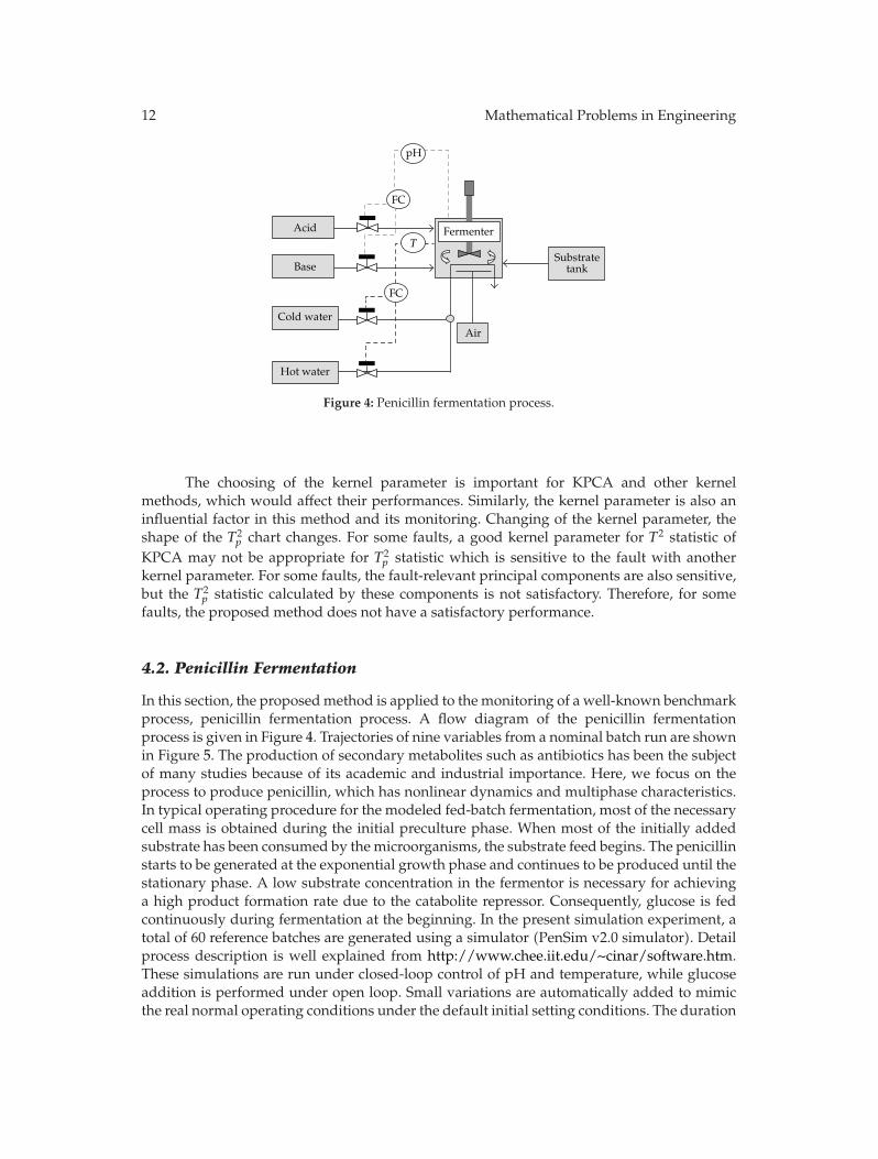
Figure 4: Penicillin fermentation process.

The choosing of the kernel parameter is important for KPCA and other kernelmethods, which would affect their performances. Similarly, the kernel parameter is also aninfluential factor in this method and its monitoring. Changing of the kernel parameter, theshape of the T2

p chart changes. For some faults, a good kernel parameter for T2 statistic ofKPCA may not be appropriate for T2

p statistic which is sensitive to the fault with anotherkernel parameter. For some faults, the fault-relevant principal components are also sensitive,but the T2

p statistic calculated by these components is not satisfactory. Therefore, for somefaults, the proposed method does not have a satisfactory performance.

4.2. Penicillin Fermentation

In this section, the proposedmethod is applied to the monitoring of a well-known benchmarkprocess, penicillin fermentation process. A flow diagram of the penicillin fermentationprocess is given in Figure 4. Trajectories of nine variables from a nominal batch run are shownin Figure 5. The production of secondary metabolites such as antibiotics has been the subjectof many studies because of its academic and industrial importance. Here, we focus on theprocess to produce penicillin, which has nonlinear dynamics and multiphase characteristics.In typical operating procedure for the modeled fed-batch fermentation, most of the necessarycell mass is obtained during the initial preculture phase. When most of the initially addedsubstrate has been consumed by themicroorganisms, the substrate feed begins. The penicillinstarts to be generated at the exponential growth phase and continues to be produced until thestationary phase. A low substrate concentration in the fermentor is necessary for achievinga high product formation rate due to the catabolite repressor. Consequently, glucose is fedcontinuously during fermentation at the beginning. In the present simulation experiment, atotal of 60 reference batches are generated using a simulator (PenSim v2.0 simulator). Detailprocess description is well explained from http://www.chee.iit.edu/∼cinar/software.htm.These simulations are run under closed-loop control of pH and temperature, while glucoseaddition is performed under open loop. Small variations are automatically added to mimicthe real normal operating conditions under the default initial setting conditions. The duration


8.63

8.62

8.61

8.6

8.59

8.58

8.570 50 100 150 200 250 300 350 400

Aeration rate (L/h)

(a)

30.2

30.1

30

29.9

29.8

29.7

29.60 50 100 150 200 250 300 350 400

Agitator power (W)

(b)

Substrate feed rate (L/h)

0.045

0.04

0.035

0.03

0.025

0.02

0.015

0.01

0.005

00 50 100 150 200 250 300 350 400

(c)

296.15

296.1

296.05

296

295.95

295.9

Substrate feed temperature (K)

0 50 100 150 200 250 300 350 400

(d)

0 50 100 150 200 250 300 350 400

80

70

60

50

40

30

20

10

0

Generated heat (kcal)

(e)

1.161.151.141.131.121.111.1

1.091.081.071.06

0 50 100 150 200 250 300 350 400

Dissolved oxygen concentration (g/L)

(f)Culture volume (L)

106

105

104

103

102

101

100

99

980 50 100 150 200 250 300 350 400

(g)

Carbon dioxide concentration (g/L)

2.5

2

1.5

1

0.5

00 50 100 150 200 250 300 350 400

(h)

Figure 5: Continued.


5.15

5.1

5.2

5.05

5

4.950 50 100 150 200 250 300 350 400

pH

(i)

Figure 5: Trajectories of nine variables from a nominal batch run.

0 50 100 150 200 250 300 350 4000

100

200

300

400

500

600

Samples

0 50 100 150 200 250 300 350 4001

1.5

2

2.5

3

3.5

4

Samples

SPEp

T2 p

×10−24


0 50 100 150 200 250 300 350 4000

0.51

1.52

2.53

3.54

4.55

Samples

0 50 100 150 200 250 300 350 400

Samples

1

1.5

2

2.5

3

3.5

4

SPE

T2

×10−24

×10−6

(b) KPCA

Figure 6: Monitoring results of the penicillin fermentation process based on (a) fault-relevant KPCA and(b) KPCA in the case of Fault 1.

of each batch is 400 h, consisting of a pre-culture phase of about 45 h and a fed-batch phase ofabout 355 h [41, 42].

The models are constructed using the proposed method. KPCA is then tested againstmonitoring of fault batches. Fault 1 is implemented by introducing a 10% step increase in theAeration rate at 100 h and retaining until 300 h. Fault 2 is implemented by introducing a 2%step increase in the Aeration rate at 100 h and retaining until 300 h. Fault 3 is implemented byintroducing a 10% step increase in the agitator power at 100 h and retaining until 300 h. Themonitoring results are shown in Figures 6, 7, and 8, respectively. As shown in Figure 6, theproposed fault-relevant KPCA method and KPCA can detect faults varying in large ranges.


0 50 100 150 200 250 300 350 4000

102030405060708090

Samples

0 50 100 150 200 250 300 350 4001.261.281.3

1.321.341.361.381.4

1.42

Samples

SPEp

T2 p

×10−24


0 50 100 150 200 250 300 350 4000123456789

Samples

0 50 100 150 200 250 300 350 4001.261.281.3

1.321.341.361.381.4

1.42

Samples

SPE

T2

×10−24

×10−7

(b) KPCA


0 50 100 150 200 250 300 350 4000

10203040506070

Samples

0 50 100 150 200 250 300 350 4002.89

2.8952.9

2.9052.91

2.9152.92

2.9252.93

2.935

Samples

SPEp

T2 p

×10−23


0 50 100 150 200 250 300 350 4000

1

2

3

4

5

6

Samples

0 50 100 150 200 250 300 350 4002.89

2.8952.9

2.9052.91

2.9152.92

2.9252.93

2.935

Samples

SPE

T2

×10−23

×10−11

(b) KPCA



In our study, when the faults vary in a small range, the proposed method can detect faultssuccessfully, but the T2 of KPCA cannot detect the faults, as shown in Figures 7 and 8.Therefore the proposed method can detect tiny fault and it is more sensitive than KPCA forthese faults.

5. Conclusions

In this article, the fault-relevant KPCA algorithm is proposed to decompose the processvariations from the fault-relevant perspective. By further decomposing the KPCA subspaces,the underlying process information can be more comprehensively looked into, which ishelpful to the detection of abnormal changes. Fault-relevant principal components extractedfrom KPCA systematic subspace and residual subspace are used to monitor the process. Withfault-relevant principal components, instead of with all principal components which maynot be influenced by the disturbances, better monitoring results are gotten. The case study onTEP and penicillin fermentation process is performed to show the performance of the fault-relevant KPCA algorithm for process monitoring. In general, swifter and more sensitive faultdetection is reported in comparison with the conventional KPCA method.

Acknowledgments

The work is supported by China’s National 973 program (2009CB320602 and 2009CB320604)and the NSF (60974057 and 61020106003).

References

[1] H. Chun-Chin and S. Chao-Ton, “An adaptive forecast-based chart for non-Gaussian processesmonitoring: with application to equipment malfunctions detection in a thermal power plant,” IEEETransactions on Control Systems Technology, vol. 19, no. 5, pp. 1245–1250, 2010.

[2] P. A. Samara, G. N. Fouskitakis, J. S. Sakallariou, and S. D. Fassois, “A statistical method for thedetection of sensor abrupt faults in aircraft control systems,” IEEE Transactions on Control SystemsTechnology, vol. 16, no. 4, pp. 789–798, 2008.

[3] T. Chen and J. Zhang, “On-line multivariate statistical monitoring of batch processes using Gaussianmixture model,” Computers and Chemical Engineering, vol. 34, no. 4, pp. 500–507, 2010.

[4] B. Zhang, C. Sconyers, C. Byington, R. Patrick, M. E. Orchard, and G. Vachtsevanos, “A probabilisticfault detection approach: application to bearing fault detection,” IEEE Transactions on IndustrialElectronics, vol. 58, no. 5, pp. 2011–2018, 2011.

[5] S. J. Qin, “Statistical process monitoring: basics and beyond,” Journal of Chemometrics, vol. 17, no. 8-9,pp. 480–502, 2003.

[6] Q. Chen and U. Kruger, “Analysis of extended partial least squares for monitoring large-scaleprocesses,” IEEE Transactions on Control Systems Technology, vol. 13, no. 5, pp. 807–813, 2005.

[7] B. Ayhan, M. Y. Chow, and M. H. Song, “Multiple discriminant analysis and neural-network-basedmonolith and partition fault-detection schemes for broken rotor bar in induction motors,” IEEETransactions on Industrial Electronics, vol. 53, no. 4, pp. 1298–1308, 2006.

[8] U. Kruger, S. Kumar, and T. Littler, “Improved principal component monitoring using the localapproach,” Automatica. A Journal of IFAC, the International Federation of Automatic Control, vol. 43, no.9, pp. 1532–1542, 2007.

[9] C. F. Alcala and S. J. Qin, “Reconstruction-based contribution for process monitoring,” Automatica,vol. 45, no. 7, pp. 1593–1600, 2009.

[10] R. Muradore and P. Fiorini, “A PLS-based statistical approach for fault detection and isolation ofrobotic manipulators,” IEEE Transactions on Industrial Electronics, vol. 59, no. 8, pp. 3167–3175, 2012.


[11] G. Li, S. J. Qin, and D. Zhou, “Geometric properties of partial least squares for process monitoring,”Automatica. A Journal of IFAC, the International Federation of Automatic Control, vol. 46, no. 1, pp. 204–210, 2010.

[12] G. Li, S. Joe Qin, and D. Zhou, “Output relevant fault reconstruction and fault subspace extraction intotal projection to latent structures models,” Industrial and Engineering Chemistry Research, vol. 49, no.19, pp. 9175–9183, 2010.

[13] J. M. Lee, C. K. Yoo, S. W. Choi, P. A. Vanrolleghem, and I. B. Lee, “Nonlinear process monitoringusing kernel principal component analysis,” Chemical Engineering Science, vol. 59, no. 1, pp. 223–234,2004.

[14] J. F. MacGregor and T. Kourti, “Statistical process control of multivariate processes,” ControlEngineering Practice, vol. 3, no. 3, pp. 403–414, 1995.

[15] G. Lee, C. Han, and E. S. Yoon, “Multiple-fault diagnosis of the Tennessee Eastman process based onsystem decomposition and dynamic PLS,” Industrial and Engineering Chemistry Research, vol. 43, no.25, pp. 8037–8048, 2004.

[16] J. M. Lee, C. Yoo, and I. B. Lee, “Statistical processmonitoringwith independent component analysis,”Journal of Process Control, vol. 14, no. 5, pp. 467–485, 2004.

[17] S. Wold, K. Esbensen, and P. Geladi, “Principal component analysis,” Chemometrics and IntelligentLaboratory Systems, vol. 2, no. 1–3, pp. 37–52, 1987.

[18] G. H. Dunteman, Principal Component Analysis, SAGE publication LTD, London, UK, 1989.[19] J. E. Jackson, A User’s Guide to Principal Component, Wiley, New York, NY, USA, 1991.[20] D. G. Kleinbaum, L. L. Kupper, and K. E. Muller, Applied Regression Analysis and Other Multivariable

Methods, Wdasworth Publishing Co Inc, California, Calif, USA, 2033.[21] A. J. Burnham, R. Viveros, and J. F. Macgregor, “Frameworks for latent variable multivariate

regression,” Journal of Chemometrics, vol. 10, no. 1, pp. 31–45, 1996.[22] B. S. Dayal and J. F. Macgregor, “Improved PLS algorithms,” Journal of Chemometrics, vol. 11, no. 1, pp.

73–85, 1997.[23] S. J. Qin, “Recursive PLS algorithms for adaptive data modeling,” Computers and Chemical Engineering,

vol. 22, no. 4-5, pp. 503–514, 1998.[24] C. Zhao, F. Wang, and Y. Zhang, “Nonlinear process monitoring based on kernel dissimilarity

analysis,” Control Engineering Practice, vol. 17, no. 1, pp. 221–230, 2009.[25] Y. W. Zhang, H. Zhou, and S. J. Qin, “Decentralized fault diagnosis of large-scale processes using

multiblock kernel principal component analysis,” Zidonghua Xuebao/ Acta Automatica Sinica, vol. 36,no. 4, pp. 593–597, 2010.

[26] Y. Zhang, H. Zhou, S. J. Qin, and T. Chai, “Decentralized fault diagnosis of large-scale processes usingmultiblock kernel partial least squares,” IEEE Transactions on Industrial Informatics, vol. 6, no. 1, pp.3–10, 2010.

[27] Y. Zhang and Z. Hu, “Multivariate process monitoring and analysis based on multi-scale KPLS,”Chemical Engineering Research and Design, vol. 89, no. 12, pp. 2667–2678, 2011.

[28] H. D. Jin, Y. H. Lee, G. Lee, and C. Han, “Robust recursive principal component analysis modeling foradaptive monitoring,” Industrial and Engineering Chemistry Research, vol. 45, no. 2, pp. 696–703, 2006.

[29] Y. H. Lee, H. D. Jin, and C. Han, “On-line process state classification for adaptive monitoring,”Industrial and Engineering Chemistry Research, vol. 45, no. 9, pp. 3095–3107, 2006.

[30] J. Yang, A. F. Frangi, J. Y. Yang, D. Zhang, and Z. Jin, “KPCA plus LDA: a complete kernel fisherdiscriminant framework for feature extraction and recognition,” IEEE Transactions on Pattern Analysisand Machine Intelligence, vol. 27, no. 2, pp. 230–244, 2005.

[31] X. Wang, U. Kruger, G. W. Irwin, G. McCullough, and N. McDowell, “Nonlinear PCA with thelocal approach for diesel engine fault detection and diagnosis,” IEEE Transactions on Control SystemsTechnology, vol. 16, no. 1, pp. 122–129, 2008.

[32] D. Zhou, G. Lee, and S. J. Qin, “Total projection to latent structures for process monitoring,” AIChEJournal, vol. 56, pp. 168–178, 2010.

[33] G. Li, C. F. Alcala, S. J. Qin, and D. Zhou, “Generalized reconstruction-based contributions for output-relevant fault diagnosis with application to the tennessee Eastman process,” IEEE Transactions onControl Systems Technology, vol. 19, no. 5, pp. 1114–1127, 2010.

[34] J. H. Cho, J. M. Lee, S. W. Choi, D. Lee, and I. B. Lee, “Fault identification for process monitoring usingkernel principal component analysis,” Chemical Engineering Science, vol. 60, no. 1, pp. 279–288, 2005.

[35] S. W. Choi, C. Lee, J. M. Lee, J. H. Park, and I. B. Lee, “Fault detection and identification of nonlinearprocesses based on kernel PCA,” Chemometrics and Intelligent Laboratory Systems, vol. 75, no. 1, pp.55–67, 2005.


[36] S. Valle, W. Li, and S. J. Qin, “Selection of the number of principal components: the variance ofthe reconstruction error criterion with a comparison to other methods,” Industrial and EngineeringChemistry Research, vol. 38, no. 11, pp. 4389–4401, 1999.

[37] S. Wold, “Cross-validatory estimation of the number of components in factor and principalcomponent models,” Technometrics, vol. 4, pp. 397–405, 1978.

[38] C. A. Lowry and D. C. Montgomery, “Review of multivariate control charts,” IIE Transactions, vol. 27,no. 6, pp. 800–810, 1995.

[39] P. Nomikos and J. F. MacGregor, “Multivariate SPC charts for monitoring batch processes,”Technometrics, vol. 37, no. 1, pp. 41–59, 1995.

[40] J. J. Downs and E. F. Vogel, “A plant-wide industrial process control problem,” Computers and ChemicalEngineering, vol. 17, no. 3, pp. 245–255, 1993.

[41] Y. Zhang and Y. Zhang, “Complex process monitoring using modified partial least squares methodof independent component regression,” Chemometrics and Intelligent Laboratory Systems, vol. 98, no. 2,pp. 143–148, 2009.

[42] Y. Zhang, S. Li, and Y. Teng, “Dynamic processes monitoring using recursive kernel principalcomponent analysis,” Chemical Engineering Science, vol. 72, pp. 78–86, 2012.

Submit your manuscripts athttp://www.hindawi.com

Hindawi Publishing Corporationhttp://www.hindawi.com Volume 2014

MathematicsJournal of


Mathematical Problems in Engineering

Hindawi Publishing Corporationhttp://www.hindawi.com

Differential EquationsInternational Journal of

Volume 2014

Applied MathematicsJournal of


Probability and StatisticsHindawi Publishing Corporationhttp://www.hindawi.com Volume 2014

Journal of


Mathematical PhysicsAdvances in

Complex AnalysisJournal of


OptimizationJournal of


CombinatoricsHindawi Publishing Corporationhttp://www.hindawi.com Volume 2014

International Journal of


Operations ResearchAdvances in

Journal of


Function Spaces

Abstract and Applied AnalysisHindawi Publishing Corporationhttp://www.hindawi.com Volume 2014

International Journal of Mathematics and Mathematical Sciences


The Scientific World JournalHindawi Publishing Corporation http://www.hindawi.com Volume 2014


Algebra

Discrete Dynamics in Nature and Society



Decision SciencesAdvances in

Discrete MathematicsJournal of

Hindawi Publishing Corporationhttp://www.hindawi.com

Volume 2014 Hindawi Publishing Corporationhttp://www.hindawi.com Volume 2014

Stochastic AnalysisInternational Journal of

Date post:	02-Jul-2018
Category:	Documents
Upload:	nguyendien
View:	226 times
Download:	0 times

Fault Detection for Industrial Processes - Hindawi...

Documents