FAULT PROGNOSIS OF BEARINGS IN ELECTRICAL DRIVES … PROGNOSIS OF BEARINGS IN ELECTRICAL DRIVES AND...

FAULT PROGNOSIS OF BEARINGS IN ELECTRICAL DRIVES AND MOTORS

By

Rodney K. Singleton II

A DISSERTATION

Submitted

to Michigan State University

in partial fulfillment of the requirements

for the degree of

Electrical Engineering – Doctor of Philosophy

2016

ABSTRACT

FAULT PROGNOSIS OF BEARINGS IN ELECTRICAL DRIVES AND MOTORS

By

Rodney K. Singleton II

In recent years, there has been a growing interest in diagnosis and prognosis of motors and elec-

trical drives. Effective and accurate diagnosis and prognosis of systems will eventually lead to

condition based maintenance, which will decrease maintenance costs and system downtime, im-

proving the reliability of electrical drives. More than 50% of motor failures are due to ball bearings.

As such, the area of bearing fault diagnosis and prognosis has attracted a lot of attention in recent

years. Although many techniques have been successfully applied for bearing fault diagnosis, prog-

nosis of faults and especially predicting the remaining useful life (RUL) of bearings is a remaining

challenge. The main reasons for this are a lack of accurate physical degradation models, limited

labeled training data, and the lack of a priori knowledge of the different health states of bear-

ings. There are several factors that contribute to bearing failure, including the mechanical stress

of a load and the electrical stress of bearing currents. Due to the intrinsic properties of motors

driven by pulse-width modulation (PWM) operation, there are current paths that form from the

motor shaft through the races of the bearing and back to ground. These current paths are caused

by voltage division interaction with the common mode voltage and stray capacitances within the

motor. One type of bearing current, electric discharge machining (EDM) current, causes a signif-

icant amount of damage to bearings. The presence of EDM currents causes pitting in the rotating

elements of the bearing and ultimately leads to bearing failure. Although this relationship is well

known and studied, little work has been done to relate bearing current discharge events to bearing

vibrations for failure prognosis.

In this work, we propose both computational and experimental approaches for RUL estimation

of bearings. In Chapter 2, we present two platforms which were used to accelerate the aging

process of bearings. The first, the PRONOSTIA Platform, accelerated bearing degradation via

excessive loads, while collecting vibration and temperature data over the course of a run. The

second platform is a new test bed we constructed to better understand the relationship between

bearing currents, vibrations and failure. This test bed applies an electrical stress on test bearings

to induce accelerated aging. Over the course of the experiments, we collect multiple sensor data

including current, temperature, and vibration from start to failure in order to correlate current data

as well as vibration data to bearing failure. In Chapter 3, we introduce an approach for learning

the hidden health states of a bearing from vibration signals. This proposed approach is based

on extracting multiple features from sensor signals and identifying change points in the state of

the system based on these features. We also propose a framework based on temporal Hidden

Markov Model for unsupervised clustering of bearing vibration data in order to identify hidden

health states in the data. In Chapter 4, we introduce a data-driven methodology, which relies on

both time and time-frequency domain features to track the evolution of bearing faults based on

vibration signals. An extended Kalman filter is applied to these features to predict the remaining

useful life and to provide a confidence interval to the RUL estimates. Performance of the proposed

methods are evaluated on the PRONOSTIA experimental test bed data. In Chapter 5, we propose

a computational framework that relates the current discharge events with the evolution of vibration

data for a more accurate RUL estimation. We use a current discharge influx event as a trigger

to perform RUL estimation on bearings using vibration data, resulting in higher accuracy and

efficiency.

This dissertation is dedicated to my grandmother, Mattie Mae Taylor.

iv

ACKNOWLEDGEMENTS

This material is based in part upon work supported by the National Science Foundation under

Grant No. EECS-1102316 and by the National Science Foundation Graduate Research Fellowship

under Grant No. DGE-0802267.

v

TABLE OF CONTENTS

LIST OF TABLES . . . . . . . . . . . . . . . . . . . . . . . . . . . . . . . . . . . . . . . viii

LIST OF FIGURES . . . . . . . . . . . . . . . . . . . . . . . . . . . . . . . . . . . . . . . ix

CHAPTER 1 INTRODUCTION . . . . . . . . . . . . . . . . . . . . . . . . . . . . . . . 1

1.1 State of the Field of Bearing Failure Prognosis . . . . . . . . . . . . . . . . . . . . 3

1.2 Contributions of the Thesis . . . . . . . . . . . . . . . . . . . . . . . . . . . . . . 7

1.3 Background . . . . . . . . . . . . . . . . . . . . . . . . . . . . . . . . . . . . . . 9

1.3.1 Time-Frequency Distributions . . . . . . . . . . . . . . . . . . . . . . . . 9

1.3.2 Time-Frequency Feature Extraction . . . . . . . . . . . . . . . . . . . . . 12

CHAPTER 2 EXPERIMENTAL DATA . . . . . . . . . . . . . . . . . . . . . . . . . . . 13

2.1 Background . . . . . . . . . . . . . . . . . . . . . . . . . . . . . . . . . . . . . . 13

2.1.1 Review of Some Previous Platforms . . . . . . . . . . . . . . . . . . . . . 13

2.1.2 Bearing Current Formation . . . . . . . . . . . . . . . . . . . . . . . . . . 15

2.1.2.1 Circulating Bearing Currents . . . . . . . . . . . . . . . . . . . . 17

2.1.2.2 Shaft Grounding Current . . . . . . . . . . . . . . . . . . . . . . 17

2.1.2.3 Electric Discharge Machining Currents . . . . . . . . . . . . . . 17

2.2 PRONOSTIA PLATFORM . . . . . . . . . . . . . . . . . . . . . . . . . . . . . . 20

2.3 Accelerated Bearing Degradation Platform via Electrical Stress . . . . . . . . . . . 23

2.4 Conclusions . . . . . . . . . . . . . . . . . . . . . . . . . . . . . . . . . . . . . . 25

CHAPTER 3 DISCOVERING THE HIDDEN HEALTH STATES FROM BEARING

VIBRATION DATA . . . . . . . . . . . . . . . . . . . . . . . . . . . . . . 26

3.1 Introduction . . . . . . . . . . . . . . . . . . . . . . . . . . . . . . . . . . . . . . 26

3.2 Hidden Health State Identification via Event Detection . . . . . . . . . . . . . . . 27

3.2.1 Feature Extraction . . . . . . . . . . . . . . . . . . . . . . . . . . . . . . 27

3.2.2 Event Detection . . . . . . . . . . . . . . . . . . . . . . . . . . . . . . . . 29

3.2.3 Results . . . . . . . . . . . . . . . . . . . . . . . . . . . . . . . . . . . . 30

3.2.3.1 Estimating the Health States . . . . . . . . . . . . . . . . . . . . 32

3.2.3.2 Performance of Multiple Features . . . . . . . . . . . . . . . . . 33

3.3 Hidden Health State Identification via Event Detection . . . . . . . . . . . . . . . 35

3.3.1 Temporal Hidden Markov Models . . . . . . . . . . . . . . . . . . . . . . 35


3.3.3 Calculating the HMM parameters . . . . . . . . . . . . . . . . . . . . . . 42

3.3.4 Unsupervised Clustering via Temporal HMM . . . . . . . . . . . . . . . . 44

3.4 Conclusions . . . . . . . . . . . . . . . . . . . . . . . . . . . . . . . . . . . . . . 48

CHAPTER 4 FAULT PROGNOSIS AND RUL ESTIMATION ON BEARINGS VIA

EXTENDED KALMAN FILTER . . . . . . . . . . . . . . . . . . . . . . . 51

4.1 Background . . . . . . . . . . . . . . . . . . . . . . . . . . . . . . . . . . . . . . 51

4.1.1 EKF Parameter Learning . . . . . . . . . . . . . . . . . . . . . . . . . . . 52

vi

4.1.2 RUL Prediction . . . . . . . . . . . . . . . . . . . . . . . . . . . . . . . . 55

4.1.3 RUL Confidence Intervals . . . . . . . . . . . . . . . . . . . . . . . . . . 56

4.1.4 RUL Estimation via Extended Kalman Filter . . . . . . . . . . . . . . . . . 56

4.1.4.1 Feature Extraction and Curve Fitting . . . . . . . . . . . . . . . 56

4.1.4.2 RUL Estimation . . . . . . . . . . . . . . . . . . . . . . . . . . 58

4.1.4.3 Comparison of EKF vs. KF . . . . . . . . . . . . . . . . . . . . 61

4.1.4.4 Confidence Interval Estimation . . . . . . . . . . . . . . . . . . 62

4.2 Conclusions . . . . . . . . . . . . . . . . . . . . . . . . . . . . . . . . . . . . . . 62

CHAPTER 5 THE USE OF BEARING CURRENTS AND VIBRATIONS IN LIFE-

TIME ESTIMATION OF BEARINGS . . . . . . . . . . . . . . . . . . . . 64

5.1 Background . . . . . . . . . . . . . . . . . . . . . . . . . . . . . . . . . . . . . . 64

5.1.1 Bearing Characteristic Frequencies . . . . . . . . . . . . . . . . . . . . . . 64

5.1.2 Data . . . . . . . . . . . . . . . . . . . . . . . . . . . . . . . . . . . . . . 64

5.2 Methodology . . . . . . . . . . . . . . . . . . . . . . . . . . . . . . . . . . . . . 65


5.2.1.1 Bearing Vibration Features . . . . . . . . . . . . . . . . . . . . . 65

5.2.2 Detection and Tracking of EDM Currents . . . . . . . . . . . . . . . . . . 66

5.2.3 RUL Prediction via EKF . . . . . . . . . . . . . . . . . . . . . . . . . . . 70

5.3 Experimental Results . . . . . . . . . . . . . . . . . . . . . . . . . . . . . . . . . 71

5.3.1 Temperature Analysis . . . . . . . . . . . . . . . . . . . . . . . . . . . . . 71

5.3.2 Comparison with Conventional Vibration Analysis . . . . . . . . . . . . . 72

5.3.3 Event-triggered RUL Estimations using Current Discharge Influx . . . . . . 74

5.4 Conclusions . . . . . . . . . . . . . . . . . . . . . . . . . . . . . . . . . . . . . . 77

CHAPTER 6 CONCLUSIONS . . . . . . . . . . . . . . . . . . . . . . . . . . . . . . . . 78

6.1 Future Work . . . . . . . . . . . . . . . . . . . . . . . . . . . . . . . . . . . . . . 79

6.1.1 Using the Hidden Health States of Bearings for Effective Fault Prognosis . 79

6.1.2 RF Detection of Bearing Discharge Events . . . . . . . . . . . . . . . . . . 80

BIBLIOGRAPHY . . . . . . . . . . . . . . . . . . . . . . . . . . . . . . . . . . . . . . . . 82

vii

LIST OF TABLES

Table 2.1 Operating Condition Specifications for the PRONOSTIA Platform . . . . . . . . 21

Table 4.1 NMSE Between Curve Fits and Features . . . . . . . . . . . . . . . . . . . . . . 57

Table 4.2 Curve Fitting Parameters for Training Data . . . . . . . . . . . . . . . . . . . . 57

Table 4.3 Comparison of RUL using Variance vs. Entropy . . . . . . . . . . . . . . . . . . 59

Table 4.4 Comparison of RUL estimations using EKF vs KF . . . . . . . . . . . . . . . . 62

Table 5.1 Bearing Characteristic Frequencies . . . . . . . . . . . . . . . . . . . . . . . . 64

Table 5.2 Comparison of RUL accuracy for training across all time versus training after

the influx event . . . . . . . . . . . . . . . . . . . . . . . . . . . . . . . . . . . 75

viii

LIST OF FIGURES

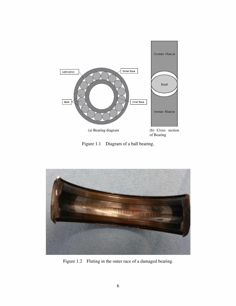
Figure 1.1 Diagram of a ball bearing. . . . . . . . . . . . . . . . . . . . . . . . . . . . . . 6

Figure 1.2 Fluting in the outer race of a damaged bearing. . . . . . . . . . . . . . . . . . . 6

Figure 1.3 Diagram of a discrete wavelet decomposition [1]. . . . . . . . . . . . . . . . . 11

Figure 2.1 Three phase voltages of an AC drive and the average of all three, or the

common mode voltage [2]. . . . . . . . . . . . . . . . . . . . . . . . . . . . . 16

Figure 2.2 Stray capacitances of an induction motor [3]. . . . . . . . . . . . . . . . . . . . 18

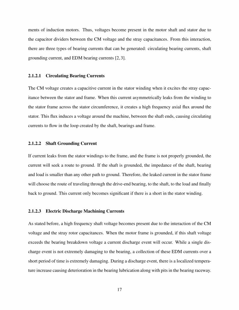
Figure 2.3 Bearing electric load states. The top row shows 3 specific voltage profiles

and their corresponding current responses are shown directly below. (a) In-

sulated. (b) Discharge. (c) Ohmic [4]. . . . . . . . . . . . . . . . . . . . . . . 20

Figure 2.4 Overview of PRONOSTIA set up [5]. . . . . . . . . . . . . . . . . . . . . . . . 22

Figure 2.5 Bearing support shaft of PRONOSTIA platform [5]. . . . . . . . . . . . . . . . 22

Figure 2.6 Comparison of new vs. degraded bearing [5]. . . . . . . . . . . . . . . . . . . . 23

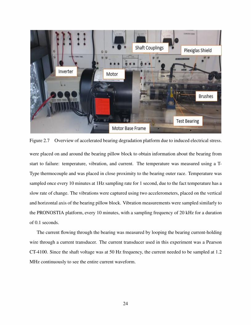
Figure 2.7 Overview of accelerated bearing degradation platform due to induced elec-

trical stress. . . . . . . . . . . . . . . . . . . . . . . . . . . . . . . . . . . . . 24

Figure 3.1 Raw Data of Initial Vibration Signal for Bearing 1 1. . . . . . . . . . . . . . . 27

Figure 3.2 Raw Data of Final Vibration Signal for Bearing 1 1. . . . . . . . . . . . . . . . 28

Figure 3.3 Choi-Williams Transformation of Initial Horizontal Vibration Signal with

σ = 10 for Bearing 1 1. . . . . . . . . . . . . . . . . . . . . . . . . . . . . . . 28

Figure 3.4 Choi-Williams Transformation of Final Horizontal Vibration Signal with σ =10 for Bearing 1 1. . . . . . . . . . . . . . . . . . . . . . . . . . . . . . . . . 29

Figure 3.5 Features for Bearing 1 1 across time. . . . . . . . . . . . . . . . . . . . . . . . 31

Figure 3.6 Change-point grouping into transition stages (shaded) for operating condi-

tions 1 and 2. . . . . . . . . . . . . . . . . . . . . . . . . . . . . . . . . . . . 33

Figure 3.7 Health state progression for Bearing 1 2. . . . . . . . . . . . . . . . . . . . . . 34

Figure 3.8 Health state progression for Bearing 2 1. . . . . . . . . . . . . . . . . . . . . . 34

Figure 3.9 Z-Score computation using 2 features on Bearing 1 2. . . . . . . . . . . . . . . 35

ix



Figure 3.12 Accelerometer results for Bearing 2 from start to failure. (a)Shows the vibra-

tions from the horizontal accelerometer for Bearing 2 and (b) the vibrations

from the vertical accelerometer for Bearing 2. . . . . . . . . . . . . . . . . . . 39

Figure 3.13 Variance of the horizontal vibration data. . . . . . . . . . . . . . . . . . . . . . 39

Figure 3.14 Raw Data of Initial Vibration Signal for Bearing 2. . . . . . . . . . . . . . . . . 40

Figure 3.15 Raw Data of Final Vibration Signal for Bearing 2. . . . . . . . . . . . . . . . . 40

Figure 3.16 Choi-Williams Transformation of Initial Horizontal Vibration Signal of Bear-

ing 2 with σ = 10. . . . . . . . . . . . . . . . . . . . . . . . . . . . . . . . . . 41

Figure 3.17 Choi-Williams Transformation of Final Horizontal Vibration Signal of Bear-

ing 2 with σ = 10. . . . . . . . . . . . . . . . . . . . . . . . . . . . . . . . . . 41

Figure 3.18 Progression of the fault for Bearing 2 in the TF domain. . . . . . . . . . . . . . 43

Figure 3.19 Features used in temporal HMM clustering for Bearing 1 across time. . . . . . . 45

Figure 3.19 cont’d . . . . . . . . . . . . . . . . . . . . . . . . . . . . . . . . . . . . . . . 46

Figure 3.20 Temporal HMM Clustering results for Bearing 1. . . . . . . . . . . . . . . . . 47



Figure 4.1 Median filtered time-domain variance across all 6 training sets for the FEMTO

data. . . . . . . . . . . . . . . . . . . . . . . . . . . . . . . . . . . . . . . . . 53

Figure 4.2 Curve fitting to variance and entropy features. . . . . . . . . . . . . . . . . . . 54

Figure 4.3 RUL Estimation for Bearing 1 3 with the variance feature. . . . . . . . . . . . . 60

Figure 4.4 RUL Estimation for Bearing 3 3 with the variance feature. . . . . . . . . . . . . 60

Figure 4.5 RUL Estimation for Bearing 2 4. . . . . . . . . . . . . . . . . . . . . . . . . . 61

Figure 4.6 RUL Estimation for Bearing 3 3 with different EKF tracking start times. . . . . 61

x

Figure 5.1 Accelerometer recordings for Bearing 1 from start to failure. (a) The vi-

brations from the horizontal accelerometer and (b) the vibrations from the

vertical accelerometer. . . . . . . . . . . . . . . . . . . . . . . . . . . . . . . . 65

Figure 5.2 Bearing current samples from Bearing 1. (a) Current sample from a bearing

under normal condition and (c) a close up of this sample. (b) Current sample

in which a discharge event has occurred and (d) a close up of this discharge event. 67

Figure 5.3 Current sample w/ discharge event and corresponding reconstructed signal

using the level 8 detail coefficients from a Haar wavelet decomposition. . . . . . 69

Figure 5.4 Normal current sample and corresponding reconstructed signal using the

level 8 detail coefficients from a Haar wavelet decomposition. . . . . . . . . . . 69

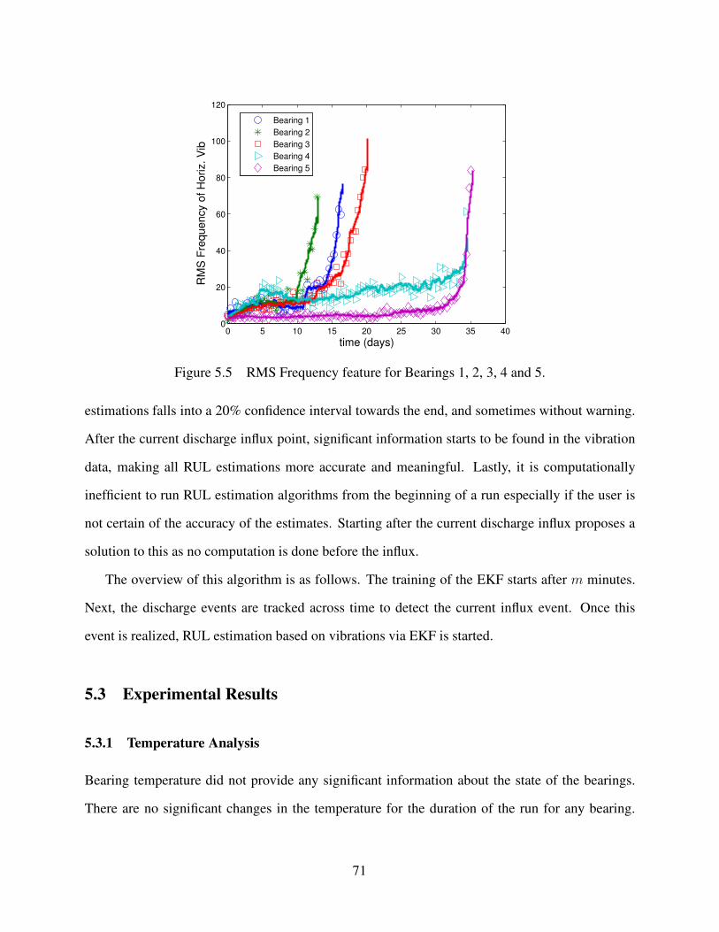
Figure 5.5 RMS Frequency feature for Bearings 1, 2, 3, 4 and 5. . . . . . . . . . . . . . . 71

Figure 5.6 Temperature signal for Bearings 1, 2, 3, 4 and 5. . . . . . . . . . . . . . . . . . 72

Figure 5.7 Relationship between bearing current discharges and vibrations for the 5 test

bearings. The first row shows the cumulative bearing discharges across the

entire run. The second row shows the RMS Frequency of the vibrations,

extracted from the frequency domain. . . . . . . . . . . . . . . . . . . . . . . . 73

Figure 5.8 Magnitude of the frequency spectrum at each bearing characteristic frequency

tracked in time for the 5 test bearings. . . . . . . . . . . . . . . . . . . . . . . 74

Figure 5.9 Detection of the current discharge influx event. The top plot shows the num-

ber of discharge events across time. The bottom plot shows the NMSE be-

tween the fitted line and the data points, with each point representing the

error over the previous m minutes. . . . . . . . . . . . . . . . . . . . . . . . . 76

Figure 5.10 RUL Estimations for Bearings 1 and 2. Each plot shows the results of starting

RUL estimations from the beginning and from the current discharge influx

event. Confidence intervals around the true RUL are shown to evaluate the

accuracy of the estimations. . . . . . . . . . . . . . . . . . . . . . . . . . . . . 76

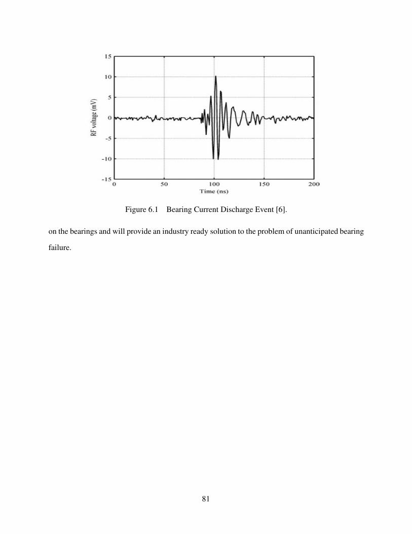
Figure 6.1 Bearing Current Discharge Event [6]. . . . . . . . . . . . . . . . . . . . . . . . 81

xi

CHAPTER 1

INTRODUCTION

Common practice in industry is to perform fixed interval maintenance as a solution to maintenance

of electromechanical systems. However, there are several problems that arise using this practice.

First, there is the possibility that failure could occur between scheduled maintenances, which could

result in a catastrophic accident. Second, performing these scheduled maintenance checks incurs

high costs, even in the case where there is no fault detected. Third, fixed interval maintenance

requires the machine to be unnecessarily out of use and unable to perform its usual function, which

is costly to the user. Condition-based maintenance, including effective diagnostic and prognostic

tools, provides a solution to this problem as maintenance only occurs when the user is alerted to

an impending failure, provided by a remaining useful life estimation [7–9].

The RUL of a system is defined as the time between the current time instant to the end of the

useful life. The concept of RUL has been widely used in reliability analysis, manufacturing sys-

tems and operational research [10, 11]. Accurate RUL predictions of electromechanical systems

will provide the user with time to get the defective part fixed or replaced. This will reduce main-

tenance costs, system downtime, and more importantly increase system safety and reliability [7].

Although there has been a lot of progress in the area of fault diagnosis using signal processing and

pattern recognition techniques [12–15], well understood systematic methodologies for prognosis

and RUL prediction from limited amount of training data are still not available.

The current approaches used for RUL estimation include model-based and data-driven meth-

ods [16,17]. The model-based approaches to prognosis use mathematical representations to incor-

porate a physical understanding of the system, and include both system modeling and physics-of-

failure (PoF) modeling. In the system modeling approach, mathematical functions or mappings,

such as differential equations, are used to represent the system. Statistical estimation techniques

based on residuals and parity relations (the difference between the model predictions and system

observations) are then used to detect, isolate and predict degradation and remaining useful life.

1

Estimation techniques such as Kalman filters and particle filters, are commonly used to calculate

the residuals [18]. For example, this approach to prognostics was demonstrated for lithium ion bat-

teries where a lumped parameter model was used along with extended Kalman filter and particle

filter algorithms to estimate remaining useful life (RUL) [19]. Physics-based failure models [20]

rely on the physics of the underlying degradation process to be able to predict the onset of failures

and are applicable in situations where accurate mathematical models can be constructed from first

principles. For example, the Yu-Harris bearing life equation [21] is commonly used to predict spall

initiation. Development of the models requires detailed knowledge of the underlying physical pro-

cesses that lead to system failure, and in complex systems, it is difficult to create dynamic models

representing the multiple physical processes occurring in the system. This is one of the limitations

of model-based approaches.

Data-driven approaches, on the other hand, use condition monitoring data coupled with artifi-

cial intelligence, e.g., neuro-fuzzy systems [22, 23], or statistical learning and pattern recognition

tools [24–26], e.g., Markov chains, hidden Markov models (HMMs) [23, 27, 28], to train a sys-

tem, and use it to estimate the RUL. Most of these techniques consist of an offline learning stage

through historical data, which includes feature extraction and degradation state learning, followed

by an online stage that continually updates the prediction of RUL, and provides an estimate of

the prediction uncertainty. In the last stage of data-driven methodologies, the learned models are

applied to test data to determine the time to the next degradation state or provide a probability of

failure. One of the advantages of data-driven approaches is that they can be used as black-box

models as they learn the behavior of the system based on monitored data and hence do not require

system-specific knowledge. Further, data-driven approaches can be applied to complex systems

since data-driven approaches can be used to model the correlation between parameters and inter-

actions between subsystems as well as effects of environmental parameters using in situ data from

the system. One of the limitations of data-driven approaches lies in the requirement of training

data. Data-driven approaches depend on historical, e.g., training, system data to determine corre-

lations, establish patterns, and evaluate data trends leading to failure. In many cases, there will be

2

insufficient historical or operational data to obtain health estimates and determine trend thresholds

for failure prognostics. A solution to this problem is to fuse system models, such as PoF models,

with the data-driven models.

In both model-based and data-driven techniques, work has been done to perform prognosis

and diagnosis through the use of intermediary health states. In most cases, there is an actual

physical meaning to the underlying health states, as in [29], where the health states correspond to

the number of damaged or missing teeth in a gear. Similarly, in [30], the number of broken rotor

bars in induction machines, which can incur many secondary effects such as mechanical vibrations,

increases in temperature, and stator winding damage [31], determines the health state of the motor.

However, problems arise when dealing with a component which does not have well-defined health

states throughout its degradation process [28]. In this case, health states need to be learned from the

data over time through event or change point detection [32]. Recently, there has been an increased

interest in event, or change-point, detection due to its ability to capture trend changes or interesting

patterns in time series data [32–34]. Moreover, these approaches can be used to partition a given

time series into different event intervals, especially when these intervals are not known a priori.

1.1 State of the Field of Bearing Failure Prognosis

Bearings are one of the most widely encountered mechanical parts in rotational equipment and

constitute a large portion of failures. Motor failures are often linked to bearing failure. Therefore,

bearing condition monitoring can be very cost effective and reduce the maintenance downtime by

providing an advance warning system that allows for the scheduling of timely corrective and repair

actions [35–37]. Traditional estimation of the lifetime of a bearing is based on the ANSI/AFBMA

Standard life rating formula [27]. However, the actual lifetime of a bearing can differ significantly

from the theoretical one due to the operating conditions. Therefore, there is a need for bearing

fault prognosis and remaining useful lifetime estimation from vibration signal analysis. Although

the bearing vibration signals contain very specific information about the bearing’s fault conditions,

3

it is quite difficult to detect and track the signature of the faults at an early stage. Moreover, the

characteristics of the fault do not necessarily progress monotonically over time which makes it hard

for standard data-driven pattern recognition approaches to succeed. Thus, one of the remaining

challenges in prognostics of bearings is how to extract the features and construct statistical tracking

algorithms from the vibration signals.

Most of the current bearing prognosis algorithms rely on different signal transforms to ex-

tract relevant features from the vibration signals in conjunction with machine learning and neural

network approaches [22, 25, 38]. However, a majority of these methods include labeled training

data to identify the different health states during the lifetime of a bearing and then build statistical

models such as Hidden Markov Models (HMMs) with parameters learned from this data [27, 28].

Moreover, most of the current prognosis algorithms that rely on probabilistic models yield the prob-

ability of transitioning to failure state in the next time step rather than an estimate of RUL [39]. In

most real life conditions, there is a lack of labeled data corresponding to the different health states

during the lifetime of the bearing. Therefore, there is no ground truth information about the timing

of the transitions between states and the total number of states.

The current state-of-the art in determining the lifetime or condition of bearing is bearing vi-

bration analysis [40, 41]. This approach is based on spectral analysis of the vibration data which

searches for the most likely frequencies present in vibration data based on the bearing’s geometry.

This analysis is used to determine a bearing fault as well as to distinguish between the different

possible fault locations, such as the inner race, outer race, etc. It can also be used as an early

warning detection method. The shortcoming of vibration analysis is that bearing vibration data is

often noisy, which leads to a complicated frequency spectrum and difficulties in analysis. In [40],

wavelet filtering is used to extract bearing characteristic frequency information from noisy vibra-

tion data, however this approach only provides early warning and not prognosis. Bearing vibrations

have been used for RUL estimation, but much less work has used the characteristic bearing fre-

quencies extracted from vibration analysis as features. In [41], particle filtering was used to track

bearing vibration features extracted from recurrence quantification analysis across time. However,

4

the major disadvantage of using vibrations for bearing fault classification and RUL estimation is

that there is little to no significant information present in the vibrations in the early stages of the

run. As the bearing degrades, the vibrations finally start to show significant changes which can

be used for accurate RUL estimations. There is also significant noise in bearing vibration read-

ings due to other components in the motor which cannot always be separated out, especially at the

beginning stages of the run of a bearing.

Although much work has been done with bearing vibrations as an indicator to bearing failure,

much less work has been done to use other types of signals such as current or voltage. Bearing

currents and their effects on bearings have been recognized as a problem for many years [42–44].

These bearing currents appear when a motor is under inverter operation and are found in one of

three forms: circulating currents, shaft grounding currents, or EDM currents [2, 3, 45]. The most

damaging type of these currents is EDM. EDM currents occur when a high voltage across the bear-

ing breaks down the lubrication film surrounding the rotating elements (see Figure 1.1). The result

is a current discharge event between the outer and inner races of the bearing. These discharge

events carry enough energy in them to cause pits and craters on the balls and the raceways of the

bearing. These craters eventually lead to fluting (see Figure 1.2), which is when the asymmetry in

the rotating elements caused by the craters leads to the balls digging deep grooves on the bearing

raceways, and the life of the bearing becomes significantly reduced [46, 47]. While this relation-

ship between bearing currents and bearing failure is well known, directly measuring these bearing

currents is physically impossible and bearing current measurements require special equipment and

personnel in normal motor operation [2, 48]. Several techniques have been developed to indirectly

measure bearing currents, including detecting them from bearing vibrations [4] and using a radio-

frequency (RF) measurement setup to detect bearing discharge events [47]. However, the challenge

of estimating or detecting bearing currents still remains.

5

(a) Bearing diagram (b) Cross section

of Bearing

Figure 1.1 Diagram of a ball bearing.

Figure 1.2 Fluting in the outer race of a damaged bearing.

6

1.2 Contributions of the Thesis

In Chapter 2, we present two different platforms from which data is collected and used in this work.

The first platform is the PRONOSTIA platform [5], which has provided an extensive vibration data

set for three types of operation for bearings loaded with radial forces. This data set has been used

by other investigators to evaluate failure prognosis and RUL estimation algorithms [36,38,49]. The

second platform presented is one we constructed that accelerates the aging process of a bearing by

applying a voltage to the bearing shaft. This induced voltage is designed in such a way that it

emulates common mode voltage from an inverter-driven motor, thus allowing EDM currents to

flow through the bearing. These EDM currents cause irreparable damage to the bearing [43, 50]

and aid in the acceleration of their degradation. The experiment is set up as follows. First, we

construct the platform to have the highest probability to exhibit severely damaging bearing current

discharge events. This worst case scenario for bearing operation entails applying a high dv/dt,

square-wave voltage to the bearing shaft with no load attached and at high speed [42]. Second, we

acquire vibration, current and temperature data from the start of the run until the bearing reaches

its failure state.

In Chapter 3, we address the problems of health state estimation from vibration data collected

from bearings. Due to the stochastic nature of bearing failures, vibration data is very noisy. More-

over, previous research has shown that bearings do not necessarily follow a monotonic degradation

pattern which makes identification of health states even more challenging and important [51]. This

part of the thesis provides two complementary approaches to extracting underlying health states

using event detection and temporal Hidden Markov Model techniques. First, we propose a new

health state estimation process for bearings using change-point detection in vibration data. These

change-points are assumed to correspond to be transitionary stages between the hidden health states

of a bearing. Next, we use a temporal Hidden Markov Model for unsupervised clustering of bear-

ing vibration data to gain a better understanding of how a bearing transitions through intermediary

stages to failure.

7

In Chapter 4, we introduce a stochastic data-driven approach that is independent from fault

severity diagnosis and that continuously updates the RUL estimate as new data samples come in.

For this purpose, we use an extended Kalman filtering based approach to first learn the degradation

trend of the extracted features from the training data, then to apply this trend to testing data to pre-

dict RUL and finally, to provide a confidence bound around the estimated RUL. We follow closely

the framework proposed by Lall et al. [52, 53] for implementing EKF for bearing RUL estimation

and offer several improvements over this implementation. First, we consider both time and time-

frequency domain features for tracking the degradation of the bearing. In the time domain, we use

the variance feature, as it has been established in the literature as a reliable indicator of the bear-

ing condition as it approaches failure. In the time-frequency domain, we propose to use a novel

entropy feature, which captures the complexity of the signal in both domains simultaneously. This

entropy feature has been shown to be a good indicator of the signal complexity and robust to time-

frequency shifts in the signal. We observe that the entropy increases as soon as the first indications

of fault develop, which relates well to the bearing Physics of Failure, where an initially localized

fault (low entropy) becomes a general roughness with high entropy. Second, we consider different

analytic models for modeling the lifetime of the bearing and build the state vectors corresponding

to each case. This enables us to fully understand how different features evolve over the lifetime of

the bearing and the effect of different model assumptions in the final RUL estimation. Third, we

provide a confidence interval for the RUL estimates using the prediction errors calculated as part

of EKF. Finally, we illustrate how different types of features may carry more information under

changing operating conditions.

Chapter 5 focuses on determining the relationship between bearing current and bearing failure,

in order to exploit this relationship for more accurate RUL estimation. Since bearing currents

are a cause of bearing failure and not an effect, tracking bearing currents over time can provide

information about an impending failure before significant changes occur in the vibration data. In

particular, it is seen that the energy of the vibration signal grows exponentially after a large influx

of bearing discharge events. This phenomenon shows that bearing currents can provide an early

8

warning to an imminent failure before there is a significant change in the bearing characteristic

frequencies used in bearing vibration analysis. In this chapter, we propose a novel approach which

first detects the current discharge events from the current sensor and then identifies critical events

during the lifetime of the bearing. These critical events are then used to determine the starting

point of RUL estimation from vibration data. In this manner, the dependence of RUL estimation

from early noisy bearing data is eliminated, the computational complexity of estimation is reduced

and the accuracy of prognosis is increased.

1.3 Background

1.3.1 Time-Frequency Distributions

Time-frequency transforms are useful for extracting information from nonstationary signals, such

as bearing vibration signals. While the Fourier transform (FT) can capture the frequency content

of stationary signals, it does not provide time-localized frequency information [54, 55]. Time-

frequency (TF) representations of signals are able to show how the spectral properties of a signal

changes over time. Although there are several methods in literature that can be used to obtain a

time-frequency representation of a signal, there is no specific transform that has distinct advantages

over the others in all circumstances [55]. Some common time-frequency transform methods are

the Short-time Fourier Transform, Wavelet transform and Cohen’s class of time-frequency distri-

butions.

The short-time Fourier Transform (STFT) is a linear TF transform that first divides the signal

of interest into multiple time segments. Fourier analysis is conducted on each time segment to

extract the frequencies that are present during that specific time window [55]. After the analysis

is completed over all time windows, the frequencies existing in the signal is shown changing over

time. The mathematical representation of the STFT is given by [56]1:

1All integrals are from −∞ to∞ unless otherwise stated.

9

S(t, ω) =

∫

f(τ)g(τ − t)e−jωtdτ, (1.1)

where f(τ) is the signal and g(t) is the sliding window which is real, symmetric and normalized.

The sliding window has a fixed length and its length introduces a trade-off between frequency and

time resolution. Long time windows result in good frequency resolution, while short time windows

provide good time resolution.

The Wavelet transform (WT) is another linear transform used to represent a signal in TF do-

main. However, instead of decomposing the signal into sinusoids at different frequencies, the WT

uses the superposition of time-shifted and scaled wavelet functions. The Discrete Wavelet Trans-

form (DWT) uses filter banks to decompose a signal into high and low frequency components [1].

First, the signal is passed through a low pass filter, h[n] and subsequently downsampled by 2. The

mathematical representation is given by [57]:

A[k] =∑

n

x[n] · h[2k − n] (1.2)

where x[n] is the signal, h[n] is the low pass filter and A[n] are called the first level approximation

coefficients. Next, the high frequency coefficients are computed using the same procedure with a

high pass filter, given by:

D[k] =∑

n

x[n] · g[2k − n] (1.3)

where g[n] is the high pass filter and D[k] are called the detail coefficients. This process provides

one level of approximation and detail coefficients. For each level afterwards, this same procedure

is iterated on the approximation coefficients of the previous level (shown in Figure 1.3).

Cohen’s class of TF distributions are quadratic TF representations and as such they are com-

putationally more expensive than STFT and WT. One of the advantages of using Cohen’s class of

time-frequency distributions is that they provide uniform resolution over both time and frequency,

while the wavelet transform does not. Cohen’s class of TFDs computes the Fourier transform of

the autocorrelation of a signal, which is the correlation of the signal with itself in both the time

and frequency domain. Since Cohen’s class of time-frequency distributions (TFDs) are not lin-

10

Figure 1.3 Diagram of a discrete wavelet decomposition [1].

ear, using these TF distributions on signals containing multiple components produces unwanted

terms. Since most signals can be broken down into multiple components, the issue of cross-terms

is prevalent in most cases. However, the effect of cross-terms can be minimized with the use of

a smoothing window, or kernel function. The kernel function acts as a filter in both time and fre-

quency [55,58,59]. The kernel function should be a low-pass filter and must be designed so that it

decreases the farther you move away from the θ−τ axis. The kernel function can be designed such

that it removes all of the cross-terms but it comes at the cost of loss in resolution [60]. Cohen’s

class of TFDs is given by [59]:

C(t, ω) =∫ ∫ ∫

φ(θ, τ)s(u+ τ2 )s∗(u− τ

2 )ej(θu−θt−τω)du dθ dτ, (1.4)

where the function φ(θ, τ) is the kernel function and s is the signal of interest. In this work, the

Choi-Williams kernel is used to filter out the cross-terms and is given by:

φ(θ, τ) = exp(−(θτ)2

σ), (1.5)

where σ controls the trade-off between time-frequency resolution and the cross-terms.

11

1.3.2 Time-Frequency Feature Extraction

From the vibration signal of bearings, time domain features including the root mean square (rms),

variance, skewness, kurtosis are commonly used in fault prognosis [36]. In the frequency domain,

commonly used features include rms frequency, frequency center, and root variance frequency [28,

35,36]. In this chapter, we focus on TF features since they are capable of jointly capturing the time

and frequency domain characteristics. As opposed to the conventional Shannon entropy, Renyi

entropy has been selected due to its ability to handle positive as well as non-positive distributions.

Renyi entropy is defined as [61]:

Hα(C) =1

1− αlog2

∑

n

∑

k

(

C[n, k]∑

n′

∑

k′ C[n′, k′]

)α

(1.6)

where α > 0 is the order, and n and k are the discrete time and frequency indices. Entropy is

well-defined for the TFD as long as∑

n

∑

k Cα[n, k] > 0.

Concentration measures have also been used to evaluate TFDs [62]. Contrary to the entropy,

concentration measure is a statistic on how concentrated a signal is and is defined as [62]:

M [C] =

∑

n

∑

k

∣

∣

∣

∣

C [n, k]∑

n′

∑

k′ C[n′, k′]

∣

∣

∣

∣

1p

p

(1.7)

where p > 1. Furthermore, small values for p, p < 4, are preferred since high p values can empha-

size small energy values disproportionately.

Lastly, common statistical moments, such as the mean, variance and skewness, can also be

extracted from the TF domain. One way to do this is to convert the time-frequency surface into

a vector and compute the well-known mean, variance, and skewness measures as defined in the

one-dimensional time domain.

12

CHAPTER 2

EXPERIMENTAL DATA

2.1 Background

2.1.1 Review of Some Previous Platforms

More than 50% of motor failures are due to ball bearings. As such, the area of bearing fault

diagnosis and prognosis has attracted a lot of attention in recent years [63,64]. Bearing degradation

can occur due to mechanical stress, resulting from sources such as radial or axial loads placed on

the bearings. Recently, research has been done to understand bearing degradation due to electrical

stress, such as the formation of EDM currents travelling through the bearing, causing mechanical

damages such as pits and races in the outer ring. In order to observe this phenomenon, several

test rigs were constructed in recent years. In [65], an experimental setup used to observe the

relationship between axial loads and the lubricating film between the tribological surfaces of deep

groove ball bearings is described. This experiment consisted of a machine with speeds of 100,

500, 1000 and 3000 RPM. Axial loads were placed on the bearings using a piezoelectric actuator

to apply force to preloaded disc springs on the outer ring of the test bearing at frequencies of 2

and 16 Hz. Each run was preceded by a 1 hour run-in period to ensure the machine had reached

a steady-state operation. After a short time in the order of milliseconds, the load was released.

The entire procedure was then repeated 10 times for each load level, varying from 100 to 800 N.

The goal of this experiment was to calculate the bearing capacitance and resulting lubricating film

thickness as inputs to the simulation model for bearing current prediction. Through this work,

the authors found that under a static load to the machine, there was a decrease in film thickness

when the bearings were exposed to low speeds and high temperatures. However, the results of the

dynamic load experiments were not trivial. In theory, one would expect to see a decrease in film

thickness as the load increased, but the results showed a near constant value of thickness spanning

13

the entire load level range. It was reasoned that this was because there was not enough time

between load changes to allow the machine to operate in steady-state. As a result, it was shown

that the main contributors to the decrease of film thickness of the bearings, thus leading to bearing

currents, are temperature and speed. As the temperature increased at any speed, the lubricating

film decreased, which theoretically leads to bearing voltage breakdown and thus bearing currents.

In [47] a test rig was constructed to explore the link between bearing vibrations and inverter-

induced bearing damage. This set-up consisted of a low-voltage, squirrel-cage induction motor

which was 3-phase, 15 kW and had 4-poles. The test bearings in this case were also deep groove

ball bearings with off-the-shelf lithium soap-based grease. The bearings were electrically insulated

from the motor and a sinusoidal voltage of 20 Vpp and 300 kHz was applied to the shaft to simulate

common mode voltage due to operation of the motor by an inverter. The signal was applied to the

shaft via a slip ring. Each bearing test was allowed to run for 1184 hours and then the experiment

was stopped. Using this test bed, the authors were able to measure the temperature of the outer

race of the bearing, the bearing voltage, bearing vibration, bearing current, and the number of

bearing discharge pulses via RF measurements. The vibration signals were sampled at 20 kHz for

400 k samples/s and the discharge activity was measured as the total number of discharges that

occurred in a 30 second window. The result was a qualitative analysis of the relationship between

vibration, temperature and bearing damage due to EDM currents. After the application of the shaft

voltage, the inner race of the test bearings appeared brand new, while the outer race exhibited

racing stripes and small craters. Although energy dissipation was attributed to the construction

of these craters, it was noted that the size of the craters should have been double in size. The

authors attributed this to the fact that the discharge activity may have occurred before the shaft

voltage reached its peak. Quantitatively, the number of RF pulses increased over time, giving a

total number of approximately 10 million discharges. It was noted that although this was a large

number, the energy dissipated in each one of these events was relatively low, around 89.15 nW,

which is not enough to cause significant bearing temperature increase. In conjunction with this

fact, the temperature readings over the course of the experiments provided insignificant information

14

pertaining to discharge activity. The vibration data provided significant results for the bearing outer

ring pass frequency and the ball rotation frequency and not the inner ring pass frequency, which

corroborated the results of the visual inspection of the test bearings after the experiments. It was

noted that the vibration data did not follow a monotonic trend, rendering it useless for quantitative

analysis.

Another test bed involving bearing currents is described in [66], in which the damage of a

bearing due to a single current pulse was examined. In this test rig, thrust ball bearings were used,

with the number of balls being manually changed from 9 to 3. Out of the 3 balls, only one was

allowed to be conductive, thus current only traveled through it and not the others. The experiments

were ran at 60, 120 and 1000 RPM. A voltage was applied across the bearing races to induce a

single current pulse on command via a circuit designed for high-frequency pulse currents. The

circuit consisted of capacitors, a resistance and power transistors and was used to simulate current

pulses delivered by a frequency converter and the driving voltage of this circuit varied from 0 to 30

Volts. Each test bearing was also loaded with an axial load of 400 N. Each experiment was run for

5 minutes with load but not applied voltage and then, subsequently, 10 minutes with current pulses

applied. The goal of this work was to analyze the visual effect of current pulses on the outer race

of a bearing, when ran at different speeds. A comparison of an image of the bearing races under a

microscope was made between a bearing with induced bearing currents and one without. For each

speed, there was a significant amount of damage that could be visibly seen under the microscope

when bearing currents were induced, and relatively less damage when they were not induced. It

was also noted that after 500 bearing current events were recorded, the average peak current was

around 2.1 A. Moreover, keeping the speed constant and increasing the driving voltage resulted in

greater damage to the bearing raceways.

2.1.2 Bearing Current Formation

Over the years, the use of variable frequency drives to control electric machines has grown due to

their capability of saving energy [66]. Modern AC drive systems create the fundamental voltage

15

Figure 2.1 Three phase voltages of an AC drive and the average of all three, or the common mode

voltage [2].

of the motor by switching a DC bus voltage onto the 3 phase terminals of the motor. In sine-

wave driven machines, the three phases of the machine are balanced and symmetric. However,

with Pulse Width Modulated (PWM) driven machines, at any point in time the only values of each

phase voltage is either +VDC or -VDC . This implies that while the inverter output voltages are

balanced and symmetric, at any instant the average of these phase voltages is nonzero [2,3,66,67].

This nonzero voltage is called the common mode (CM) voltage and is between the stator neutral

and frame ground. The frequency of this CM voltage can be in the kHz to MHz scale, as it is equal

to switching frequency of the inverter. An example of the three phase outputs to the machine and

their corresponding neutral is shown in Figure 2.1.

CM voltage affects the stator, rotor, shaft, and bearings through the stray capacitances of the

motor. These capacitances are created inherently through the separation of the conducting ele-

16

ments of induction motors. Thus, voltages become present in the motor shaft and stator due to

the capacitor dividers between the CM voltage and the stray capacitances. From this interaction,

there are three types of bearing currents that can be generated: circulating bearing currents, shaft

grounding current, and EDM bearing currents [2, 3].

2.1.2.1 Circulating Bearing Currents

The CM voltage creates a capacitive current in the stator winding when it excites the stray capac-

itance between the stator and frame. When this current asymmetrically leaks from the winding to

the stator frame across the stator circumference, it creates a high frequency axial flux around the

stator. This flux induces a voltage around the machine, between the shaft ends, causing circulating

currents to flow in the loop created by the shaft, bearings and frame.

2.1.2.2 Shaft Grounding Current

If current leaks from the stator windings to the frame, and the frame is not properly grounded, the

current will seek a route to ground. If the shaft is grounded, the impedance of the shaft, bearing

and load is smaller than any other path to ground. Therefore, the leaked current in the stator frame

will choose the route of traveling through the drive-end bearing, to the shaft, to the load and finally

back to ground. This current only becomes significant if there is a short in the stator winding.

2.1.2.3 Electric Discharge Machining Currents

As stated before, a high frequency shaft voltage becomes present due to the interaction of the CM

voltage and the stray rotor capacitances. When the motor frame is grounded, if this shaft voltage

exceeds the bearing breakdown voltage a current discharge event will occur. While a single dis-

charge event is not extremely damaging to the bearing, a collection of these EDM currents over a

short period of time is extremely damaging. During a discharge event, there is a localized tempera-

ture increase causing deterioration in the bearing lubrication along with pits in the bearing raceway.

17

Figure 2.2 Stray capacitances of an induction motor [3].

These pits over time lead to craters and fluting (shown in Figure 1.2) in the bearing raceway, which

signifies bearing damage. Under sine-wave operation, the shaft voltage necessary to exceed the

bearing breakdown voltage threshold is significantly lower than under PWM operation. Because

of this, the resulting EDM current under PWM inverter operation are higher and more damaging

to bearings [42].

The bearing breakdown voltage is determined by the lubrication in the bearing. The character-

istics of the lubrication are dependent on a number of factors, including the grease conductivity,

motor speed, motor load, and bearing voltage [43,45]. First, the conductive grease in bearings can

act as a suppressant to EDM currents. Since these currents are a result of the potential difference

between the balls and the races, conducting grease removes that potential difference. However, the

authors in [45] found that conductive grease only has this effect on bearings for the first 40 hours

of operation. After this time, conductive grease behaves similarly to nonconducting grease, giving

way to electric discharges. Second, the speed of the rotating elements in the bearing has an effect

18

on the lubrication film thickness. At low speeds, the lubrication film is thin, causing metal-to-metal

and quasi-metal surface contact, allowing circulating and discharge currents to flow freely through

the bearing. Because the lubrication film is thin, these discharge events do not contain much en-

ergy and minimally damage the bearing. At high speeds, a thicker lubrication film is built, which

significantly increases the resistance between the bearing raceways, leading to less metal-to-metal

contact points. In order for current to flow through the bearing, the bearing voltage has to be large

enough to exceed the bearing breakdown voltage, consequently producing more damaging electric

discharge events than at lower speeds. Third, both the rate of change of the voltage amplitude

have significant influence on the presence of electric discharge events. Shaft voltages with high

dv/dt place high stress on the lubrication, causing breakdowns and thus discharges. Under PWM

operation, the breakdown threshold voltage is between 8 - 15 V under 60 Hz operation, which

produces high energy discharge events causing severe damage. Last, the load associated with the

motor has minimal effect on the presence of EDM currents. However, the presence of a load on

bearings increases their life expectancy as unloaded bearings present the worst case scenario for

bearing discharge currents [42, 43, 68].

Due to the intrinsic properties of bearings previously discussed, there are three probable states

a bearing can manifest. Those states are shown in Figure 2.3, with insulated, discharge, and the

ohmic in which the current has a 180◦ phase shift in 2.3a, 2.3b, and 2.3c, respectively [4]. The

first state, referred to as insulated, is when the bearing acts purely capacitive and allows no current

to flow. This occurs when there is a sufficient amount of lubrication separating the balls and

the races. The second state, referred to as discharge, occurs when there is a breakdown in the

previously capacitive state, causing the bearing capacitor to discharge creating an influx of current.

The third state, or ohmic state, is when the current flowing through the bearing follows the trend of

the shaft voltage. The bearing is purely resistive in this state due to metal-to-metal contact between

the balls and the races or conducting lubrication grease.

19

a) Insulated

Vol

tage

b) Discharge c) Ohmic

Cur

rent

Figure 2.3 Bearing electric load states. The top row shows 3 specific voltage profiles and their

corresponding current responses are shown directly below. (a) Insulated. (b) Discharge. (c) Ohmic

[4].

2.2 PRONOSTIA PLATFORM

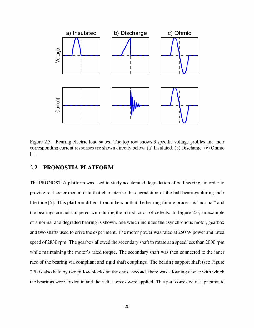
The PRONOSTIA platform was used to study accelerated degradation of ball bearings in order to

provide real experimental data that characterize the degradation of the ball bearings during their

life time [5]. This platform differs from others in that the bearing failure process is ”normal” and

the bearings are not tampered with during the introduction of defects. In Figure 2.6, an example

of a normal and degraded bearing is shown. one which includes the asynchronous motor, gearbox

and two shafts used to drive the experiment. The motor power was rated at 250 W power and rated

speed of 2830 rpm. The gearbox allowed the secondary shaft to rotate at a speed less than 2000 rpm

while maintaining the motor’s rated torque. The secondary shaft was then connected to the inner

race of the bearing via compliant and rigid shaft couplings. The bearing support shaft (see Figure

2.5) is also held by two pillow blocks on the ends. Second, there was a loading device with which

the bearings were loaded in and the radial forces were applied. This part consisted of a pneumatic

20

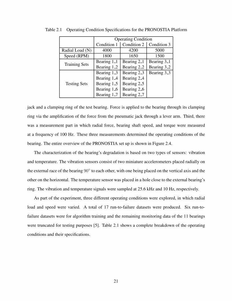
Table 2.1 Operating Condition Specifications for the PRONOSTIA Platform

Operating Condition

Condition 1 Condition 2 Condition 3

Radial Load (N) 4000 4200 5000

Speed (RPM) 1800 1650 1500

Training SetsBearing 1 1 Bearing 2 1 Bearing 3 1

Bearing 1 2 Bearing 2 2 Bearing 3 2

Testing Sets

Bearing 1 3 Bearing 2 3 Bearing 3 3

Bearing 1 4 Bearing 2 4




jack and a clamping ring of the test bearing. Force is applied to the bearing through its clamping

ring via the amplification of the force from the pneumatic jack through a lever arm. Third, there

was a measurement part in which radial force, bearing shaft speed, and torque were measured

at a frequency of 100 Hz. These three measurements determined the operating conditions of the

bearing. The entire overview of the PRONOSTIA set up is shown in Figure 2.4.

The characterization of the bearing’s degradation is based on two types of sensors: vibration

and temperature. The vibration sensors consist of two miniature accelerometers placed radially on

the external race of the bearing 90◦ to each other, with one being placed on the vertical axis and the

other on the horizontal. The temperature sensor was placed in a hole close to the external bearing’s

ring. The vibration and temperature signals were sampled at 25.6 kHz and 10 Hz, respectively.

As part of the experiment, three different operating conditions were explored, in which radial

load and speed were varied. A total of 17 run-to-failure datasets were produced. Six run-to-

failure datasets were for algorithm training and the remaining monitoring data of the 11 bearings

were truncated for testing purposes [5]. Table 2.1 shows a complete breakdown of the operating

conditions and their specifications.

21

Figure 2.4 Overview of PRONOSTIA set up [5].

Figure 2.5 Bearing support shaft of PRONOSTIA platform [5].

22

Figure 2.6 Comparison of new vs. degraded bearing [5].

2.3 Accelerated Bearing Degradation Platform via Electrical Stress

The experimental procedure in this test bed resulted in accelerated degradation of a bearing by

inducing a current through its races. The induced bearing current produced an electrical stress on

the bearing causing a breakdown in the lubrication film surrounding the balls in the ball bearing.

This accelerated bearing degradation platform included a 3-phase induction machine connected

to a pillow block bearing through a piece-wise shaft, including several couplings. The induction

machine was electrically isolated from the bearing shaft via a nylon shaft coupling connected to the

motor output shaft. The insulated piece of the shaft was then coupled to a copper tube, or bearing

shaft, via a High-Speed Bellows Flexible Shaft Coupling. Lastly, the bearing was then fit on to the

copper tube, with no load attached to the shaft. Brushes were placed on the bearing shaft in order

to provide a contact point to apply a voltage. A plexiglas shield was placed over the couplings as

a safety measure. An overview of the setup is shown in Figure 2.7.

A voltage was applied to the shaft, from the bearing inner race to outer race using a voltage

buffer amplifier circuit. This shaft voltage was a 20 Vpp pulse with a 50 kHz frequency. For each

experiment, the induction machine was run at 2400 RPM with an inverter. Three types of sensors

23

Figure 2.7 Overview of accelerated bearing degradation platform due to induced electrical stress.

were placed on and around the bearing pillow block to obtain information about the bearing from

start to failure: temperature, vibration, and current. The temperature was measured using a T-

Type thermocouple and was placed in close proximity to the bearing outer race. Temperature was

sampled once every 10 minutes at 1Hz sampling rate for 1 second, due to the fact temperature has a

slow rate of change. The vibrations were captured using two accelerometers, placed on the vertical

and horizontal axis of the bearing pillow block. Vibration measurements were sampled similarly to

the PRONOSTIA platform, every 10 minutes, with a sampling frequency of 20 kHz for a duration

of 0.1 seconds.

The current flowing through the bearing was measured by looping the bearing current-holding

wire through a current transducer. The current transducer used in this experiment was a Pearson

CT-4100. Since the shaft voltage was at 50 Hz frequency, the current needed to be sampled at 1.2

MHz continuously to see the entire current waveform.

24

2.4 Conclusions

In this chapter, we discussed the importance of studying bearing failure as it contributes to over

half of motor failures. We also discussed the causes of bearing failure, including excessive radial

and axial loads, temperature and electrical stress via bearing current flow. Bearing current flow can

come in 3 different forms: circulating currents, shaft grounding currents, or EDM currents. EDM

currents are damaging to bearings and create pits and craters on the rotating elements of bearings.

These craters lead to fluting and eventually bearing failure. To observe this, we presented a new

test bed which allows the accelerated degradation of bearings. An electrical stress is placed on

the bearings by applying a voltage to the bearing shaft, allowing current flow through the bearing.

Over the course of the experiment, we collected temperature, vibration and current data. We also

provided information about a separate test bed, the PRONOSTIA platform, which used excessive

loads to accelerate the aging process of the bearing. In the subsequent chapters, data from these

two test beds are analyzed and features are extracted in order to perform RUL estimation.

In future work, more bearings should be tested using the platform we constructed in order to

collect more data. This will help to obtain a collection of historical data for bearing fault prognosis.

Furthermore, a solution to measure bearing current in real-world motor setups should be developed.

Future work should also develop methodologies for detecting bearing currents indirectly, using

either an RF system or bearing current estimation techniques from measured bearing voltage [47,

69]. This will give way to practically implementable RUL estimation for bearings that can be used

in industry, as a means to prevent system downtime or motor failure due to bearing failure.

25

CHAPTER 3

DISCOVERING THE HIDDEN HEALTH STATES FROM BEARING VIBRATION DATA

3.1 Introduction

Bearing fault diagnosis and prognosis has been a growing area of interest, since bearing failure

causes more than 50% of motor failure cases. Previous works have found success in the area of

fault diagnosis and prognosis by utilizing health states to discern the state of a system’s degradation

[29–31]. However, bearing health states are not defined by a physical phenomenon. In this chapter,

we explore the problem of health state estimation from vibration data for bearing fault prognosis.

There has been much work done in using health states as a means to failure prognosis. In [29],

Hidden Markov Models (HMM) was used to conduct prognosis on gear failures. An HMM was

trained on the training data and the learned states were used to classify testing data into a particular

health state. The HMM was then used to predict the next probable state and provided a warning

if the next state was the failure state. However, in this work, each health state had a physical

meaning, as each state corresponded to a different number of broken teeth. However, for systems

which contain no distinct physical phenomena contributing to specific health states, there is a need

for unsupervised clustering. In [70], hierarchical HMMs were used to conduct both supervised and

unsupervised clustering on acoustic data. Similarly, HMMs were used in [71] to cluster ecology

data into classes. However, there still remains the issue of finding the hidden health states in

bearing vibration data.

In this chapter, we propose two different methodologies to address this issue. The first is a novel

unsupervised clustering method based on an event detection framework which identifies periods

of stationarity in the data. These periods of stationarity are then used to partition the data into

several health states. Although this approach can successfully and effectively cluster the data into

meaningful states, it is purely heuristic. The second approach uses a more statistical framework, a

temporal hidden Markov model, to partition the data into classes. These hidden health states can

26

0 0.02 0.04 0.06 0.08 0.1−2

0

2

4

Horizontal Raw Vibration Data

Time (s)A

ccel

erat

ion

0 0.02 0.04 0.06 0.08 0.1−2

−1

0

1

2

Vertical Raw Vibration Data

Time (s)

Acc

eler

atio

n

Figure 3.1 Raw Data of Initial Vibration Signal for Bearing 1 1.

be used to diagnose the condition of a bearing, and subsequently estimate the next probable state.

3.2 Hidden Health State Identification via Event Detection

3.2.1 Feature Extraction

The vibration data from the PRONOSTIA platform, described in Chapter 2, is used for feature

extraction in this section. An example of raw vibration signals from the initial (healthy state)

and final (failure) sample can be found in Figures 3.1 and 3.2. In the time domain, variance

was extracted as a feature. In Figure 4.1, we can see the progression of the variance across time

for each of the training datasets. Since the vibrations are known to be nonstationary, we also

considered TF domain features such as entropy with α = 2 (see eqn. 1.6). The raw vibration

signals were transformed into the TF domain using the Choi-Williams distribution with σ = 10.

The TF representations of initial and failure samples are shown in Figures 3.3 and 3.4, respectively.

From the TFD, we observed that the vertical vibration TF representation gave little useful

information. We noticed two phenomena that were evident across all training sets in the horizontal

data as the fault progressed. First, there was a shift from a significant amount of concentrated

27

0 0.02 0.04 0.06 0.08 0.1−40

−20

0

20

40

Horizontal Raw Vibration Data

Time (s)

Acc

eler

atio

n

0 0.02 0.04 0.06 0.08 0.1−40

−20

0

20

40

Vertical Raw Vibration Data

Time (s)

Acc

eler

atio

n

Figure 3.2 Raw Data of Final Vibration Signal for Bearing 1 1.

Horizontal Vibrations

time (sec)

Freq

uenc

y (H

z)

5000 10000 15000 20000 25000

40

80

120

160

200

240

−0.2

−0.15

−0.1

−0.05

0

0.05

0.1

0.15

0.2

Figure 3.3 Choi-Williams Transformation of Initial Horizontal Vibration Signal with σ = 10 for

Bearing 1 1.

28

Horizontal Vibrations

time (sec)

Freq

uenc

y (H

z)

5000 10000 15000 20000 25000

40

80

120

160

200

240

−0.2

−0.15

−0.1

−0.05

0

0.05

0.1

0.15

0.2

Figure 3.4 Choi-Williams Transformation of Final Horizontal Vibration Signal with σ = 10 for

Bearing 1 1.

energy, at the start, to impulsive energy distribution, at failure, in the 160-200 Hz frequency band.

Second, there was a shift from insignificant energy to a large amount of energy in the 236-256 Hz

and 0-40 Hz frequency bands. These three frequency bands were explored in feature extraction,

using entropy and concentration measures [72–74] to capture these trends and the resulting features

had clear trends across time.

3.2.2 Event Detection

Event detection is used to determine a change in the data to signify different health states. There

are many different ways to determine these change points, but in this work we utilize the Z-score

as defined in [32]. First we constructed a feature matrix, Φ ∈ RF×T , where F is the number

of features and T is the total number of time points. Next, we constructed F × F , time-varying

correlation matrices, C(t), from Φ, using sliding windows of length W where:

Cij(t) =

∣

∣

∣

∣

ρX,Y =E[(X− µX)(Y− µY)]

σXσY

∣

∣

∣

∣

(3.1)

where X and Y are localized feature matrices Φ(i, t −W : t) and Φ(j, t −W : t), respectively.

From these time-varying correlation matrices C(t), we computed the principal eigenvector, u(t).

29

This vector u(t) summarizes the activity of each feature in that time interval and is given by solving

the equation:

(C(t)− λmaxI)u(t) = 0, i, j ∈ 1, 2, . . . F , (3.2)

where I is an F × F identity matrix and λmax is the maximum solution of

det(C(t)− λI) = 0. (3.3)

In order to determine the change-points, this vector u(t) is compared to an average of all the

previous W ′ principal eigenvectors, denoted as r(t − 1) = 1W ′

W ′∑

i=1u(t − i). The Z-score is given

as Z(t) = 1 − u(t)T r(t − 1). Thus, if u(t) ∈ RF×1 is dramatically different from r(t− 1), their

dot product will be 0, producing a Z-score of 1. If u(t) and r(t − 1) are similar, their dot product

will be close to 1, producing a Z-score close to 0. Since u(t) and r(t− 1) are both unit vectors, the

Z-score is always between 0 and 1. Finally, change points can be detected as spikes, or high scores

in the plot of the Z-score.

3.2.3 Results

In this work, from the FEMTO data, we extracted a total of 6 features from the TF domain (shown

in Figure 3.5):

1) Entropy from the 160-200 Hz frequency band


3) Concentration measure from the 0-40 Hz frequency band

4) Variance from the 236-256 Hz frequency range

5) Mean from the 236-256 Hz frequency range

6) Skewness from the 236-256 Hz frequency range

In the event detection step, a window size of W = W ′ = 100 samples was used across all

six training sets. It is assumed that a change-point occurs in a particular training set if the Z-score

30

0 500 1000 1500 2000 2500 3000−2

−1

0

1

2

3

4

5

time (samples)

Ske

nw

ess

Skewness of 236−256 Hz Band

(a) Skewness of 236-256 Hz Band

0 500 1000 1500 2000 2500 3000−5

−4

−3

−2

−1

0

1

2

En

tro

py

Entropy of 160−200 Hz Band

time (samples)

(b) Entropy of 160-200 Hz Band

0 500 1000 1500 2000 2500 3000−5

−4

−3

−2

−1

0

1

2

Entr

opy

time (samples)

Entropy of 236−256 Hz Band

(c) Entropy of 236-256 Hz Band

0 500 1000 1500 2000 2500 3000−1

0

1

2

3

4

5

6

7

Variance of 236−256 Hz Band

time (samples)

Va

ria

nce

(d) Variance of 236-256 Hz Band

0 500 1000 1500 2000 2500 3000−1

0

1

2

3

4

5

6

7

Me

an

Mean of 236−256 Hz Band

time (samples)

(e) Mean of 236-256 Hz Band

0 500 1000 1500 2000 2500 3000−1.5

−1

−0.5

0

0.5

1

1.5

2

Co

nce

ntr

atio

n M

ea

su

re

Concentration Measure of 0−40 Hz Band

time (samples)

(f) Concentration Measure of 0-40 Hz Band

Figure 3.5 Features for Bearing 1 1 across time.

31

increases beyond a threshold, given by µ(Zni)+σ(Zni

) where Zni= [Z1Z2 . . . Zni ] and ni is the

number of samples in the ith training set, µ is the mean and σ is the standard deviation across all

time.

3.2.3.1 Estimating the Health States

Applying the proposed change point detection algorithm to different training sets corresponding

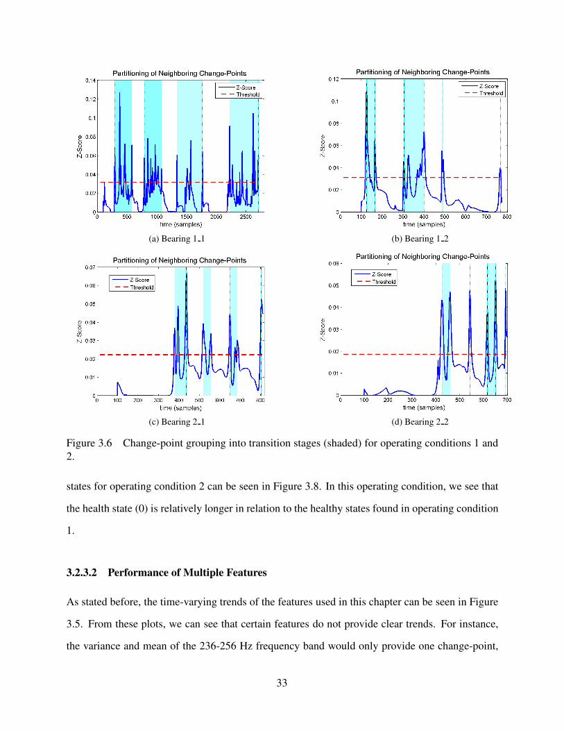
to different operating conditions yielded different transitions between health states. For example,

in Figure 3.6 we can see the Z-score results for the first two operating conditions. We noticed that

across time, the two training sets within the same operating condition showed similar trends but

they were distinctly different from the trend of the other operating condition. We also noticed that

there were groups of change-points in close proximity to each other as well as periods of little

change throughout all training datasets. We reason that multiple change-points within a window

correspond to a transition stage from one state to the next. In other words, time periods where there

were great changes in the data (i.e. multiple change-points over a short time period) were called

transitionary states. Conversely, the time periods where there are no change-points correspond to

the actual health states. An example of this partitioning of the time series data for Bearing 1 1,

in the first operating condition, can be found in Figure 3.6a, where the shaded areas represent the

transition stages and the unshaded represent the estimated health states. The other training set in

this operating condition had a similar trend in its Z-score plot over time, as can be seen in Figure

3.6b. Given these similar grouping trends from operating condition 1, we can build a complete

overview of health states and transition stages of the bearing from start to failure, as seen in Figure

3.7. In this overview, we can see 5 distinct health states and 4 transitionary stages between them.

From this, we can determine that there is a healthy state (0), 3 intermediary health states (1-3), and

the failure state (4).

The Z-score trends for the two training datasets in operating condition 2 can be seen in Figure

3.6c and 3.6d. These training sets provided a different trend from the first operating condition,

which could be attributed to the different load speeds and forces. An overall view of the health

32

(a) Bearing 1 1 (b) Bearing 1 2

(c) Bearing 2 1 (d) Bearing 2 2

Figure 3.6 Change-point grouping into transition stages (shaded) for operating conditions 1 and

2.

states for operating condition 2 can be seen in Figure 3.8. In this operating condition, we see that

the health state (0) is relatively longer in relation to the healthy states found in operating condition

1.

3.2.3.2 Performance of Multiple Features

As stated before, the time-varying trends of the features used in this chapter can be seen in Figure

3.5. From these plots, we can see that certain features do not provide clear trends. For instance,

the variance and mean of the 236-256 Hz frequency band would only provide one change-point,

33

0 100 200 300 400 500 600 700 8000

1

2

3

4

5

time (samples)

Hea

lth S

tate

Health State Progression

Figure 3.7 Health state progression for Bearing 1 2.

0 100 200 300 400 500 600 700 800 9000

1

2

3

4

5

time (samples)

Hea

lth S

tate

Health State Progression

Figure 3.8 Health state progression for Bearing 2 1.

while others, such as the two entropy features, would result in multiple change-points due to their

fluctuations.

In this section, we evaluate the use of different number of features for change point detec-

tion. For instance, in Figure 3.9, we can see the effect of computing the Z-score using only two

(skewness of 236-256 Hz band and entropy of 160 - 200 Hz band) of these 6 features for Bearing

1 2. The Z-Score is high throughout the entire training set. This is because it is hard to detect

change-points in signals with high volatility, such as bearing vibration data. However, when we

34

0 100 200 300 400 500 600 700 8000

0.1

0.2

0.3

0.4

0.5

0.6

0.7

0.8

0.9

1

time (samples)

Z−S

core

Z−Score using two variables

Figure 3.9 Z-Score computation using 2 features on Bearing 1 2.

use more features, we can see that the change-point detection algorithm becomes more robust to

noise and can identify more distinct change-points. This phenomenon can be seen as the features

increase from 2 to 6 in increments of 2. Figure 3.10 shows the Z-score for the algorithm which

utilizes 4 features (skewness, entropy of both freq. bands, and the variance of 236-256 Hz band).

In this plot, we can see that the change-points become more conspicuous. Furthermore, as the

number of features is increased to 6, seen in Figure 3.11, the change-points become even more

apparent, as some change-points towards the beginning of the run are combined into one, showing

that there is a direct relationship between the number of features used and the ease of identifying

the change-points.

3.3 Hidden Health State Identification via Event Detection

3.3.1 Temporal Hidden Markov Models

The HMM is a statistical method and has been extensively used in the modeling and analyzation

of stochastic processes. The HMM has been used in a variety of applications such as speech

recognition [75], motor fault diagnosis [29, 76], and bearing failure prognosis [23]. The HMM is

used to model systems which have a finite number of hidden states (S1, S2, . . . SM ) which are each

35

0 100 200 300 400 500 600 700 8000

0.01

0.02

0.03

0.04

0.05

0.06

0.07

time (samples)

Z−S

core

Z−Score using four variables

Z−Score

Threshold


0 100 200 300 400 500 600 700 8000

0.02

0.04

0.06

0.08

0.1

0.12

time (samples)

Z−S

core

Z−Score using six variables

Z−Score

Threshold


indirectly observable via the sequence of observations, (O = o1, o2, . . . oN ), they exhibit. There

are three parameters that govern the HMM:

1) An initial probability matrix, π, which determines the initial probability of a given state,

mathematically represented as

πi = P (q0 = Si), 1 ≤ i ≤M, (3.4)

where q0 is the first state in a state sequence.

36

2) A state transition probability matrix, A = aij , which gives the probability of a state Sj given

the previous state was Si, where

aij = P (qt = Sj |qt−1 = Si). (3.5)

3) An observation probability matrix, B = bj(ot), which determines how likely an observation

is given the state is Sj , where

bj(ot) = P (ot|qt = Sj) (3.6)

For simplicity, an HMM can be written as λ = (π,A,B). However, there is a limitation in using

HMM for time-series data since HMM assumes that each observation is statistically independent of

the previous. For time-series data, this is usually not the case. The temporal HMM was proposed to

avoid this limitation by assuming that each observation is statistically dependent on its predecessor.

If we assume a finite number of observable states, (W = w1, w2, . . . wk), the probability of ot

taking the value wt is given by

P (ot = wt|ot−1 = wt−1, ot−2 = wt−2, . . . o1 = w1) = P (ot = wt|ot−1 = wt−1). (3.7)

This is similar to a first order Markov process in that the probability of an observation at time t

only depends on the observation at time t − 1. Using this condition, the observation probability

matrix is updated to contain two parameters, q and p, where q(i) = P (o1 = wi) and p(i, j) =

P (ot = wj|ot−1 = wi). It is noted that these parameters must satisfy the conditions

N∑

i=1

q(i) = 1,N∑

j=1

p(i, j) = 1 1 ≤ i, j,≤ N. (3.8)

.

The probabilities q and p can be calculated using [77]

37

q(i) =1

L

L∑

i=1

P (wi|o(l)t , λ) (3.9)

and

p(i, j) =

∑Ll=1

∑Tlt=2 P (Si|o

(l)t−1, λ)P (Sj|o

(l)t λ)

∑Ll=1

∑Tlt=2 P (Si|o

(l)t−1, λ)

, (3.10)

where 1 ≤ i, j ≤ N, 1 ≤ l ≤ L, L is the number of training sequences, Tl is the length of the lth

observation sequence, and P (Si|o(l)t , λ) is the posterior probability of a particular state, Si, given

a observation sequence, o(l)t and HMM model, λ. Once these parameters, which characterize the

HMM model, are defined, the probability of an observation sequence, with length T , is calculated

as [77]

P (O|λ) =∑

S

P (O, S|λ) =∑

S

P (O|S, λ)P (S|λ), (3.11)

where

P (O|S, λ) = q(o1 = w1|S, λ)T∏

t=2

p(ot = wt|ot−1 = wt−1, S, λ) (3.12)

and

P (S|λ) = P (S1|λ)

T∏

t=2

P (St|St−1, λ) = πS1

T∏

t−2

aSt−1St. (3.13)


The vibration data from the accelerated bearing degradation platform via electrical stress, described

in Chapter 2, is used for feature extraction in this section. The vibrations from this experiment fol-

lowed a similar trend as those in the PRONOSTIA setup. At the beginning of the run, the amplitude

of the vibrations is at its smallest point. At the end of the run, when the bearing moves towards

failure, the vibrations increase exponentially (see Figure 3.12). The variance of the vibrations also

increases exponentially over the duration of a run (shown in Figure 3.13). Thus, the variance of

38

(a) Horizontal Accelerometer (b) Vertical Accelerometer

Figure 3.12 Accelerometer results for Bearing 2 from start to failure. (a)Shows the vibrations

from the horizontal accelerometer for Bearing 2 and (b) the vibrations from the vertical accelerom-

eter for Bearing 2.

Figure 3.13 Variance of the horizontal vibration data.

the vibrations is again selected as a feature. An example of raw vibration signals from the initial

(healthy state) and final (failure) sample can be found in Figures 3.14 and 3.15, respectively.

Their corresponding TF representations, using the Choi-Williams distribution with σ = 10, can be

found in Figures 3.16 and 3.17, respectively. As the fault progresses, there is a significant amount

of energy in the 80 - 90 Hz frequency band. This may be due to the rotational speed of the motor

being 80 Hz. As the bearing nears failure, the energy across the surface becomes more impulsive.

39

Figure 3.14 Raw Data of Initial Vibration Signal for Bearing 2.

Figure 3.15 Raw Data of Final Vibration Signal for Bearing 2.

We also saw little energy distribution in the 20 - 80 Hz frequency band until the bearing reached

failure. In Figure 3.18, snapshots of the Bearing 2 run from start to failure in the TF domain is

shown. These frequency bands, as well as the energy over the entire TF plane, were used for fea-

ture extraction. Entropy and concentration measures were again used to capture the changes in

the spread of energy in the TF domain across time. In the time domain, the first four statistical

moments, mean, variance, skewness and kurtosis were extracted. In the frequency domain, the

max, variance and RMS were also chosen as features. Finally, in the TF domain, the concentration

40

Time (seconds)

Freq

uenc

y (H

z)

Horizontal Vibrations in TF Domain

0 0.02 0.04 0.06 0.08 0.10

20

40

60

80

100

120

(m/s

2 )2

−0.4

−0.3

−0.2

−0.1

0

0.1

0.2

0.3

Figure 3.16 Choi-Williams Transformation of Initial Horizontal Vibration Signal of Bearing 2

with σ = 10.

Time (seconds)

Freq

uenc

y (H

z)


0 0.02 0.04 0.06 0.08 0.10

20

40

60

80

100

120(m

/s2 )2

−0.4

−0.3

−0.2

−0.1

0

0.1

0.2

0.3

Figure 3.17 Choi-Williams Transformation of Final Horizontal Vibration Signal of Bearing 2

with σ = 10.

41

measure over the entire TF plane, and entropy from the 80-90 Hz frequency band and the entire

TF plane were extracted as features.

3.3.3 Calculating the HMM parameters

In this section, we will describe how each parameter of the HMM is calculated from the selected

features.

1) The initial probability vector, π, and the state transition matrix, A.

First, the number of classes, K, is set arbitrarily at the beginning. In this work, we selected a

range of three to five classes. Next, a k-NN classification is run on the feature matrix, classifying

the feature vector at each time point into one of K states. The initial probability vector, π, is

initialized using the ratio of the number of feature vectors in each state to the total number of

feature vectors given as

πi =Ki

N, (3.14)

where Ki is the number of feature vectors in the ith class and N is the total number of feature

vectors. The probabilities of the state transition matrix, A, are then calculated in a brute force

manner, where aij is given by the number of times a feature vector is found in state j at time t,

given the state at time t− 1 was i, divided by the total number of feature vectors.

2) The observation probability matrix, B = (q, p).

To calculate the parameters of the observation probability matrix, the features are first quantized

to the nearest tenth to create a finite number of observable outcomes, W = (w1, w2, . . . wk). The

transitional probabilities, p(i, j) = P (ot = wt|ot−1 = wt−1) are again calculated in a brute force

manner similar to the calculation of A, being

42

Time (seconds)

Fre

quency (

Hz)


0 0.02 0.04 0.06 0.08 0.10

20

40

60

80

100

120

(m/s

2)2

−0.4

−0.3

−0.2

−0.1

0

0.1

0.2

0.3

(a) Initial Sample

Time (seconds)

Fre

quency (

Hz)


0 0.02 0.04 0.06 0.08 0.10

20

40

60

80

100

120

−0.4

−0.3

−0.2

−0.1

0

0.1

0.2

0.3

(b) Intermediate Sample (1)

Time (seconds)

Fre

quency (

Hz)


0 0.02 0.04 0.06 0.08 0.10

20

40

60

80

100

120

−0.4

−0.3

−0.2

−0.1

0

0.1

0.2

0.3

(c) Intermediate Sample (2)

Time (seconds)

Fre

quency (

Hz)


0 0.02 0.04 0.06 0.08 0.10

20

40

60

80

100

120

−0.4

−0.3

−0.2

−0.1

0

0.1

0.2

0.3

(d) Intermediate Sample (3)

Time (seconds)

Fre

quency (

Hz)


0 0.02 0.04 0.06 0.08 0.10

20

40

60

80

100

120

−0.4

−0.3

−0.2

−0.1

0

0.1

0.2

0.3

(e) Intermediate Sample (4)

Time (seconds)

Fre

quency (

Hz)


0 0.02 0.04 0.06 0.08 0.10

20

40

60

80

100

120

(m/s

2)2

−0.4

−0.3

−0.2

−0.1

0

0.1

0.2

0.3

(f) Final Sample

Figure 3.18 Progression of the fault for Bearing 2 in the TF domain.

43

p(i, j) = P (ot = wt|ot−1 = wt−1) =Number of times observation wt directly follows wt−1

Total number of observations

(3.15)

3.3.4 Unsupervised Clustering via Temporal HMM

The proposed method was applied to the data from the accelerated bearing degradation via electri-

cal stress platform. In this work, we extracted a total of 11 features from the TF domain (shown in

Figure 3.19):

1) Variance over the entire surface of the TF representation


3) Entropy over the entire surface of the TF representation

4) Concentration measure over the entire surface of the TF representation

5) Max magnitude from the frequency domain

6) Variance from the frequency domain

7) RMS from the frequency domain

8) Mean from the time domain

9) Variance from the time domain

10) Skewness from the time domain

11) Kurtosis from the time domain

The parameters of the HMM were calculated as outlined in section 3.3.3. For this work, we

chose to look at K = 3, 4, and 5 clusters. After performing the unsupervised clustering of the

vibration data, we can see a trend in the transitions of the hidden health states across all bearings

as we increase the number of classes.

In Figure 3.20(a), the clustering results for Bearing 1 are shown, withK = 3. As the number of

classes increases to four (shown in Figure 3.20(b)) and five (shown in Figure 3.20(c)), the classes

44

0 2 4 6 8 10 12 14 16 18

−1

0

Mean (

Norm

aliz

ed)

time (days)

Mean

(a) Mean from the time domain

0 2 4 6 8 10 12 14 16 18−1

0

1

2

3

4

5

Variance (Time Domain)

time (days)

Variance (

Norm

aliz

ed)

(b) Variance from the time domain

0 2 4 6 8 10 12 14 16 18−2

−1

0

1

2

Skew

ness (

Norm

aliz

ed)

Skewness

time (days)

(c) Skewness from the time domain

0 2 4 6 8 10 12 14 16 18−2

−1

0

1

2

3

4

Kurt

osis

(N

orm

aliz

ed)

time (days)

Kurtosis

(d) Kurtosis from the time domain

0 2 4 6 8 10 12 14 16 18−1

0

1

2

3

4

5

Variance (Freq. Domain)

time (days)

Variance (

Norm

aliz

ed)

(e) Variance from the frequency domain

0 2 4 6 8 10 12 14 16 18−1

0

1

2

3

4

RMS Frequency

time (days)

RM

S F

req. (N

orm

aliz

ed)

(f) RMS from the frequency domain

Figure 3.19 Features used in temporal HMM clustering for Bearing 1 across time.

45

Figure 3.19 cont’d

0 2 4 6 8 10 12 14 16 18−1

0

1

2

3

4

Max. Frequency

time (days)

Max. F

req. (N

orm

aliz

ed)

(g) Max from the frequency domain

0 2 4 6 8 10 12 14 16 18−4

−3

−2

−1

0

1

2

3

time (days)

Concentration Measure over Entire Surface

Concentr

ation M

easure

(N

orm

aliz

ed)

(h) Concentration measure over the entire surface of the TF

representation

0 2 4 6 8 10 12 14 16 18−3

−2

−1

0

1

2

3

time (days)

Entropy over Entire Surface

Entr

opy (

Norm

aliz

ed)

(i) Entropy over the entire surface of the TF representation

0 2 4 6 8 10 12 14 16 18−3

−2

−1

0

1

2

time (days)

Entropy of 80−90Hz bandE

ntr

opy (

Norm

aliz

ed)

(j) Entropy from the 80-90 Hz frequency band

0 2 4 6 8 10 12 14 16 18−1

0

1

2

3

4

5

6

Variance (TF Domain)

time (days)

Variance (

Norm

aliz

ed)

(k) Variance over the entire surface of the TF representation

46

0 2 4 6 8 10 12 14 16 181

2

3

Bearing 1 − 3 StatesS

tate

s

time (days)

(a) 3 States

0 2 4 6 8 10 12 14 16 181

2

3

4

Bearing 1 − 4 States

Sta

tes

time (days)

(b) 4 States

0 2 4 6 8 10 12 14 16 181

2

3

4

5

Bearing 1 − 5 States

Sta

tes

time (days)

(c) 5 States

Figure 3.20 Temporal HMM Clustering results for Bearing 1.

become unevenly distributed, with the majority of classes at the end of the run. This trend is also

shown in Figures 3.21, 3.20 for Bearings 2 and 4, respectively.

In Bearing 4 the first class divides into two states as we increase the number of clusters from 3

to 4. Although this is slightly contrary to the trend, there are still more transitions between classes

at the end of the run when the number of clusters is increased to 5. This analysis is congruent with

what is happening physically in the bearing and its vibrations. As the bearing nears failure, more

significant information is found, thus requiring more states to capture the changing trend.

47

0 2 4 6 8 10 12 141

2

3

Bearing 2 − 3 ClassesS

tate

s

time (days)

(a) 3 Classes

0 2 4 6 8 10 12 141

2

3

4

Bearing 2 − 4 Classes

Sta

tes

time (days)

(b) 4 Classes

0 2 4 6 8 10 12 141

2

3

4

5


Sta

tes

time (days)

(c) 5 Classes


3.4 Conclusions

In this chapter, we have introduced two complementary methods for hidden health state estima-

tion in bearing vibration data. First, we proposed a multivariate event detection framework to

learn the hidden health states of bearings from unlabeled training data. We have shown that these

health states are not necessarily discrete and evolve continuously over time. Moreover, we have

shown how including more relevant features for health state estimation improves the accuracy and

increases the reliability of state estimation. We also showed that different operating conditions re-

48

0 5 10 15 20 25 30 351

2

3

Bearing 4 − 3 ClassesS

tate

s

time (days)

(a) 3 Classes

0 5 10 15 20 25 30 351

2

3

4


Sta

tes

time (days)

(b) 4 Classes

0 5 10 15 20 25 30 351

2

3

4

5


Sta

tes

time (days)

(c) 5 Classes


sulted in contrasting state transition profiles, alluding to the need for prognosis to be conducted on

an operating condition specific basis. Second, we introduced an unsupervised clustering method

based on temporal HMM clustering to obtain the hidden health states of a bearing when degraded

by electrical stress. As the number of classes increase, there is less separation between the lat-

ter classes. This corresponds to the physical process of bearing degradation, in which significant

changes in the data occur towards failure.

In future work, discovering hidden health states may improve the current state of the art di-

agnosis and prognosis methods. Once the different health states are identified, typical RULs for

49

each health state can be determined from training data. This information along with representative

features corresponding to each state can provide a probabilistic way of estimating the RUL from

new testing data. Furthermore, the temporal HMM clustering method can be used on other types

of sensor data, such as current, and fused across different sensors. The hidden health states found

in this analysis can be compared to the results using only vibration signals to determine any corre-

lations. Lastly, more historical data is needed to assure the certainty of this method across all types

of bearings and operating conditions.

50

CHAPTER 4

FAULT PROGNOSIS AND RUL ESTIMATION ON BEARINGS VIA EXTENDED

KALMAN FILTER

4.1 Background

Kalman filtering is a recursive algorithm that estimates the true state of a system based on noisy

measurements. The Kalman filter has been used in many applications involving navigation, on-

line system identification and tracking [78, 79]. Recently, Kalman filtering has been successfully

applied to fault prognosis [52]. For example, in [30], Kalman filtering is used to interpolate the

signal feature trends learned from the labeled data and then to estimate the evolution of the faults

for diagnosis purposes. However, Kalman filtering assumes a linear system dynamics model with

Gaussian noise in the measurements which is not always realistic in real life applications. Ex-

tended Kalman Filtering (EKF) is an extension of this framework to nonlinear system dynamics

and has been used by Lall et al. [52, 53] for prognostics of electronic interconnects and by Saha

et al. [80] for battery life management. The EKF equation in the presence of process noise and

measurement noise is:

xk = f(xk−1, uk−1) + wk−1 (4.1)

where xk is the state being estimated, f is a nonlinear function of states, uk is the input at time

sample k, wk is random zero mean noise with covariance matrix Qk. In EKF, the relationship

between system states (xk) and measurements (zk) can also be nonlinear:

zk = h(xk) + vk, (4.2)

where zk is the measurement, h is a measurement function which is a nonlinear function of states

and vk is zero-mean random process described by the measurement noise covariance matrix, Rk.

In order to carry out the normal Kalman Filter operations, the nonlinear functions, f and h, must be

locally linearized around the estimated state by calculating their respective Jacobian, producing the

matrices F and H, respectively. One important point in the implementation of EKF is the choice

51

of the initial parameters, as the speed of convergence depends on the initial estimate, x0 and the

uncertainty matrix, P0 [81].

4.1.1 EKF Parameter Learning

For the two different types of features, i.e. vibration and entropy, time dependent degradation

models are obtained through curve fitting. For example, for the variance feature, an exponential

of the form aebt was found to be the most suitable whereas for the time-frequency entropy feature

a curve in the form of a − be−ct was more suitable (see Figures 4.2a and 4.2b). The parameters

of the degradation function are updated with each new measurement. To accomplish this, a state

vector x containing the equation for the curve fit as well as the unknown parameters describing

this degradation model at each time point are defined for each feature. For the variance feature, the

parameters ak and bk of the exponential curve are used to define the state vector as [51, 82]:

xk = [aebk a b]T (4.3)

and for the entropy feature:

xk = [ak − bke−ckk ak bk ck]

T , (4.4)

both with the measurement equation given by:

zk = h(xk) = xk(1). (4.5)

It is also noted that there is no input to this system, so in our case uk defined in equation 4.1 is

equal to zero . With each time step, the parameters of the degradation model are updated to form a

new model, fk, and an estimate of the next state, xk is calculated. The functions f and h are then

locally linearized about that estimate to produce Fk and Hk by:

Fk =∂f

∂x

∣

∣

∣

∣

xk

=

0 ebkk kakebkk

0 1 0

0 0 1

, (4.6)

52

0 500 1000 1500 2000 2500 30000

2

4

6

8

10

12

14

16

18

20Variance − Training Set 1

Samples

Variance

(a) Bearing 1 1

0 100 200 300 400 500 600 700 800 9000

0.2

0.4

0.6

0.8

1

1.2

1.4

1.6

1.8

2Variance − Training Set 2

Samples

Variance

(b) Bearing 1 2

0 200 400 600 800 10000

0.2

0.4

0.6

0.8

1

1.2

1.4Variance − Training Set 3

Samples

Variance

(c) Bearing 2 1

0 100 200 300 400 500 600 700 8000

0.1

0.2

0.3

0.4

0.5

0.6

0.7

0.8


Samples

Variance

(d) Bearing 2 2

0 100 200 300 400 500 6000

0.1

0.2

0.3

0.4

0.5

0.6


Samples

Variance

(e) Bearing 3 1

0 200 400 600 800 1000 1200 1400 1600 18000

0.2

0.4

0.6

0.8

1

1.2


Samples

Variance

(f) Bearing 3 2

Figure 4.1 Median filtered time-domain variance across all 6 training sets for the FEMTO data.

53

0 0.5 1 1.5 2 2.5 3

x 104

0

5

10

15

20

25

30

35

40

45

50

time (sec)

Variance (

(m/s

2)2

)Curve Fit for Variance Feature

Variance Data

Curve Fit

(a) Variance curve fit for Bearing 1 1

0 1000 2000 3000 4000 5000 60000

2

4

6

8

10

12

time (sec)

Entr

opy (

bits)

Curve Fit for Entropy Feature

Entropy Data

Curve Fit

(b) Entropy curve fit for Bearing 3 1

Figure 4.2 Curve fitting to variance and entropy features.

Hk =∂h

∂x

∣

∣

∣

∣

xk

=

[

1 0 0

]

, (4.7)

for the variance trend and

Fk =∂f

∂x

∣

∣

∣

∣

xk

=

0 1 −e−ckk kbke−ckk

0 1 0 0

0 0 1 0

0 0 0 1

, (4.8)

Hk =∂h

∂x

∣

∣

∣

∣

xk

=

[

1 0 0 0

]

, (4.9)

for the entropy trend.

The initial state estimate given to the EKF, x0, consisting of the initial value for the degradation

feature as well as the initial guesses for the parameters was found through use of the training

data. Averages of these values within operating conditions were then used as the initial parameter

estimates in x0 in the RUL prediction stage. Furthermore, the initial values for each training set

was extracted and the average for each operating condition was used as the initial value for the

54

degradation feature in x0. The initial uncertainty matrix, P0, was chosen empirically as:

P0 =

0.1 0 0

0 0.1 0

0 0 0.1

(4.10)

4.1.2 RUL Prediction

The failure thresholds, γi, where γi is the ith threshold for a given operating condition, were

extracted as the value at the final sample of each training dataset. The final testing threshold for

each operating condition was computed as the average of these per operating condition, given by:

γo =1

K

K∑

i=1

γi, (4.11)

where K is the number of training sets in operating condition o. Tracking of the test features

begins after a certain amount of time has passed since the data at the first time points are not

usually reliable for RUL estimation and may not follow the trend learned from the training data.

An overall view of the algorithm and all its steps are given below:

1) Initialize x0 and P0.

2) Predict the next state, xk, and uncertainty matrix, Mk:

xk = f(xk−1) + wk−1, (4.12)

Mk = Fk−1Pk−1Fk−1 + Qk−1. (4.13)

3) Take in measurement, zk.

4) Update the predictions and their uncertainties using the Kalman gain, Kk:

Kk = MkHTk

(

HkMkHTk + Rk

)−1, (4.14)

xk ←− xk + Kk(zk −Hkxk), (4.15)

55

Pk = (1−KkHk)Mk. (4.16)

5) The current value of the feature state is extrapolated out to failure threshold. The total number

of time steps, n, required to reach the failure threshold is taken as the RUL at time k.

γo = xk+n = fk(xk+n−1) + wk+n (4.17)

6) Calculate the confidence intervals of RUL predictions (see section III-E).

7) Repeat process starting at step 3.

4.1.3 RUL Confidence Intervals

An important aspect of prognosis is not just to predict the RUL, but to add a confidence measure

to it as well. In the testing phase, the confidence interval of the RUL prediction is calculated

by using the error covariance matrix, P. At the end of each step, the error covariance matrix

is updated giving the uncertainty measurement between the predicted state, x and the true mea-

surement. Since the first value in the state variable is the actual feature value, being either en-

tropy or variance, P(1, 1) contains the uncertainty of the predicted state. Given this uncertainty,

a 95% confidence interval can be placed around the estimate and the upper and lower bounds,

xubd = x(1) + 2.567P(1, 1) and xlbd = x(1) − 2.567P(1, 1), are extracted. Similar to original

RUL estimation, these values can also be extrapolated to the failure threshold to obtain upper and

lower confidence bounds on the RUL predictions.

4.1.4 RUL Estimation via Extended Kalman Filter

4.1.4.1 Feature Extraction and Curve Fitting

For all of the datasets described in Table I, both time domain variance and time-frequency domain

entropy features are extracted. A degradation trend is extracted from the training data based on

these features by analytical curve fitting. The accuracy of curve fitting was quantified by the

normalized mean square error (NMSE), given by‖x−x‖2‖x‖2

, where x is the fitted curve and x is the

56

Table 4.1 NMSE Between Curve Fits and Features

Operating Condition Training set Entropy Variance

11 0.0510 0.3525

2 0.0434 0.3326

23 0.0537 0.7146

4 0.0515 0.5462

35 0.0335 0.8422

6 0.0485 0.3680

Table 4.2 Curve Fitting Parameters for Training Data

Operating Training Entropy Variance

Condition Set a b c a b

11 9.296 1.286 0.3661 1.429e−40 0.03397

2 9.434 1.832 0.4021 5.556e−15 0.03916

23 9.963 8.92 0.01413 0.1862 0.001592

4 10.2 7.509 0.007981 0.1349 0.002287

35 9.747 8.593 0.037 3.026e−8 0.03364

6 8.851 4.694 0.007381 1.181e−65 0.09228

raw data. For the variance feature, it was noted that the first and third operating conditions behave

similarly, with the degradation trend modeled by an exponential function aebt across the lifetime

of the bearings. The average NMSE across the four training sets in operating conditions 1 and 3 for

the variance feature is 0.526. However, for the second operating condition, the degradation trend

for the variance feature in the testing data does not fit the trend learned from the training data. This

may be due to the fact that the testing samples provided for operating condition 2 were truncated

before the variance feature could capture the degradation, i.e. the testing life history is shorter,

average of 152 minutes, compared to the other operating conditions. For the entropy feature, we

determined the best curve fit to be of the form a − be−ct, and the average NMSE between this fit

and the entropy from all the training sets was 0.048. Table 4.1 shows all of the NMSE values for

both features and all training sets. Table 4.2 shows the values of the parameters for each training

set. We also note that the NMSE is usually higher for the variance feature since its range is larger

compared to entropy as seen in Figure 4.2.

57

4.1.4.2 RUL Estimation

As noted above, we used two different features in order to estimate the RUL based on the operating

condition. In Table 4.3, the RUL estimation results using entropy versus variance on all of the

testing datasets are given. The results are quantified by the percentage of RUL estimations that fall

within +/− 20% of the true RUL in the last 500 seconds. It is shown that using variance in the 1st

and 3rd operating conditions will provide the user with accurate RUL estimations towards the end

of the test sets. However, the variance feature cannot predict the true RUL for operating condition

2. This is due to the fact that the variance feature, as shown in Figure 4.2a, stays constant all the way

through the run until the very end, where it is able to capture the failure of the bearing. Therefore,

if the testing dataset is truncated too early, i.e. before the bearing gets close to failure, the variance

feature is not a good indicator of failure and cannot perform well in the subsequent RUL estimation.

On the other hand, the entropy feature shows an initial increase in value, indicative of the bearing’s

health deterioration, and then stays stable around this value as shown in Figure 4.2b. As such, when

the test set is short compared to the lifetime of the bearing, as in the case of operating condition

2, the entropy feature is successful in tracking the early deterioration of bearing health and in

predicting the true RUL in most of the test cases. When the test data set is longer, entropy does not

yield accurate RUL estimates since during the last 500 seconds of the lifetime of the bearing the

entropy values do not change that much. Therefore, in the final analysis, the variance feature was

used for operating conditions 1 and 3, and the entropy feature was used for operating condition 2.

It is also important to note that for certain test sets from condition 2, in particular for Bearing 2 3

and Bearing 2 7, neither feature gets close to the true RUL estimate. This is due to the fact that the

test data set is very short, e.g. only 29 minutes in the case of Bearing 2 7.

In particular, Figure 4.3a shows the results of RUL predictions on bearing 1 3. Predictions

were started at the half point since early RUL predictions with the variance feature are not very

reliable and meaningful. As shown in this figure, the RUL predictions at the beginning have a lot

of error but as time goes on they converge to the true RUL. Figure 4.4 shows the RUL estimations

58

Table 4.3 Comparison of RUL using Variance vs. Entropy

Operating Condition Test set Duration (min) Variance Entropy

1

1 300 96% 0%

2 190 100% 0%

3 384 46% 0%

4 384 54% 0%

5 250 40% 0%

2

6 200 0% 4%

7 102 0% 70%

8 334 0% 24%

9 95 0% 36%

10 29 0% 0%

3 11 59 56% 0%

over time for the only testing set in the third operating condition, bearing 3 3. Here, too, we can

see that the trend of RUL predictions across time converges to the true RUL line. It is noted that

the convergence of this set is slower than that of the previous. This is due to the lack of substantial

number of samples for updating, i.e. shorter test data set (59 minutes). Figure 4.5 illustrates the

performance of the entropy feature in RUL prediction for bearing 2 4 from the second operating

condition. Although the dataset is more truncated compared to the other two operating conditions,

entropy is able to track the actual RUL value.

We also noticed in the RUL prediction algorithm that the time at which EKF tracking is started

has an effect on how quickly the estimated RULs converge to the true RUL. If the tracking is

started at the beginning of the testing data, the convergence is much slower as there is more irrel-

evant samples or noise in the data that lowers the accuracy of the RUL prediction. An example

of this phenomena can be seen in Figure 4.6, where we show the RUL estimations of the same

bearing with different start times for tracking. The convergence of the algorithm is faster when the

procedure is started midway, instead of at the very beginning. Neither one of these starting points

converges as fast as starting past halfway, as seen in Figure 4.4.

59

0 0.5 1 1.5 2

x 104

0

1

2

3

4

5

6

7x 10

4

time (sec)

RU

L (

sec)

RUL predictions for bearing 1_3

Predicted RUL

True RUL

(a) RUL prediction over time versus the actual RUL

16500 17000 17500 180000

2000

4000

6000

8000

10000

12000

14000

16000

18000

20000

time (sec)

RU

L (

sec)

RUL predictions for bearing 1_3 (closeup)

Predicted RUL

95% Confidence Bounds

True RUL

20% Confidence Intervals

(b) Confidence interval for the estimated RUL near end of

testing

Figure 4.3 RUL Estimation for Bearing 1 3 with the variance feature.

0 500 1000 1500 2000 2500 3000 3500 40000

1

2

3

4

5

6

7

8

9x 10

4

time (sec)

RU

L (s

ec)


Predicted RUL

True RUL

Figure 4.4 RUL Estimation for Bearing 3 3 with the variance feature.

60

0 100 200 300 400 500 600 7000

0.5

1

1.5

2

2.5

3

3.5x 10

4

time (sec)

RU

L (s

ec)


Predicted RUL

True RUL

20% confidence Intervals

Figure 4.5 RUL Estimation for Bearing 2 4.

3100 3150 3200 3250 3300 3350 3400 3450 3500

0

2000

4000

6000

8000

10000

12000

14000

16000

time (sec)

RU

L (s

ec)


From Beginning

From Middle

True RUL

Figure 4.6 RUL Estimation for Bearing 3 3 with different EKF tracking start times.

4.1.4.3 Comparison of EKF vs. KF

In this section, we compare the performance of the proposed Extended Kalman Filter (EKF) ap-

proach to the regular Kalman Filter (see Table 4.4), which is commonly used in literature for

prognosis, in terms of the percentage of estimated RUL values within +/− 20% of the true RUL

in the last 500 seconds. For the majority of the datasets, the Kalman Filter (KF) shows no accuracy

towards the end of the testing dataset with the exception of test set 6. Overall, EKF based RUL

algorithm performs better than the KF for all operating conditions.

61

Table 4.4 Comparison of RUL estimations using EKF vs KF

Operating Condition Test set EKF KF

1

1 96% 0%

2 100% 0%

3 46% 0%

4 54% 0%

5 40% 0%

2

6 4% 92%

7 70% 8%

8 24% 0%

9 36% 4%

10 0% 24%

3 11 56% 0%

4.1.4.4 Confidence Interval Estimation

In Figure 4.3b, we can see a closer view of the end of the run, along with the confidence intervals

of the RUL estimations. We also show a bandwidth around the true RUL (+/- 20% of the true RUL

value) to see how well the estimated RULs fall within this band. At the beginning of the algorithm,

the true RUL is not within the confidence bounds of the predictions. This is due to the fact that

samples towards the beginning of the testing data may not provide enough information to perform

feature tracking. However, towards the end of the run, the predictions as well as their confidence

intervals are both within 20% of the actual RUL.

4.2 Conclusions

In this chapter, we have introduced an Extended Kalman Filtering based approach for tracking the

RUL of bearings. First, we introduced both time and time-frequency domain features of vibration

signals and illustrated that different features may work better under different operating conditions.

Second, we gave a detailed description of RUL estimation based on EKF along with a procedure

to estimate the confidence interval along the RUL estimates. Finally, we applied the proposed

algorithm to bearing vibration data to illustrate the convergence of the algorithm along with its

behavior under different conditions.

62

Future work should consider several improvements to our RUL estimation methodology. First,

as the results indicate the starting point of EKF in the testing data has a direct effect on the con-

vergence rate of the RUL estimates. Future work should consider sliding window based EKF

implementation such that at each time point only the most recent past time points are used to esti-

mate the RUL. This type of an approach may help with fitting the learned trend of the degradation

profile to the testing features. Since the testing data is a truncated version of the full lifetime of

a bearing, the trends obtained for training data may not always be good fits to the testing data

resulting in large amount of prediction error. Second, future work should consider fusion of differ-

ent features and corresponding degradation profiles for a more accurate system model. Moreover,

different pre-processing methods to the data should be explored. Third, future work should con-

sider alternative approaches to learning the degradation models from extracted data such as neural

networks. Finally, the proposed framework should be extended to different types of sensor data,

such as the current, from bearings to improve the RUL estimation accuracy.

63

CHAPTER 5

THE USE OF BEARING CURRENTS AND VIBRATIONS IN LIFETIME ESTIMATION

OF BEARINGS

5.1 Background

5.1.1 Bearing Characteristic Frequencies

Due to the nature of the rotating elements of bearings, specific frequencies have been shown to be

present in frequency analysis of bearing vibrations. These bearing characteristic frequencies are

calculated from the geometry of the bearing and are given in Table 5.1, where d is the diameter of

the rolling elements,D is the pitch circle diameter, Z is the number of rolling elements and α is the

contact angle. These equations are only valid if the rotating elements do not exhibit any sliding,

which is usually not the case in most applications [83].

5.1.2 Data

The data in this chapter comes from the accelerated degradation platform via electrical stress,

described in Chapter 2.

Table 5.1 Bearing Characteristic Frequencies

Fundamental train freq. relative to outer ringfr2

[

1− dcosαD

]

Fundamental train freq. relative to inner ringfr2

[

1 + dcosαD

]

Ball pass freq. of outer ring Z fr2

[

1− dcosαD

]

Ball pass freq. of inner ring Z fr2

[

1 + dcosαD

]

Rotating element spin freq.Dfr2d

[

1−(

dcosαD

)2]

64

0 2 4 6 8 10 12 14 16 18−50

−40

−30

−20

−10

0

10

20

30

40

50

Bearing 1 Raw Horiz. Vib.

time (days)

Accele

ration (

m/s

2)

(a) Horizontal Accelerometer

0 2 4 6 8 10 12 14 16 18−50

−40

−30

−20

−10

0

10

20

30

40

50

Bearing 1 Raw Vert. Vib.

time (days)

Accele

ration (

m/s

2)

(b) Vertical Accelerometer

Figure 5.1 Accelerometer recordings for Bearing 1 from start to failure. (a) The vibrations from

the horizontal accelerometer and (b) the vibrations from the vertical accelerometer.

5.2 Methodology


5.2.1.1 Bearing Vibration Features

At the beginning of the run, the amplitude of the vibrations is at its smallest point. At the end

of the run, when the bearing starts to fail, the amplitude of the vibrations increases exponentially

(see Fig. 5.1). Some common features extracted from bearing vibration data to capture trends

are statistical moments, such as variance, from the time domain and RMS frequency from the

frequency domain [28, 35, 36, 84]. In this chapter, the RMS frequency feature is chosen, given by:

RMS Freq. =

√

√

√

√

1

n

n∑

i=1

(∣

∣Xfft,i

∣

∣)2, (5.1)

where n is the number of frequency samples and Xfft,i is the ith sample of the Fourier transform

of the vibration signal.

65

5.2.2 Detection and Tracking of EDM Currents

In these experiments, the bearings are found to be mostly in the ohmic state, in which the bearing

current follows the same behavior as the bearing shaft voltage. Fig. 5.2a shows a normal current

sample without any discharge events. In Fig. 5.2c, a closeup plot of the normal bearing current is

shown and it can be seen that the trend is pulse-like resembling the shaft voltage. As the bearing

degrades, it begins switching between the three electrical states: ohmic, capacitive and discharge.

In Fig. 5.2b, a current sample for the same bearing at a later time is shown. In this time period, a

spike occurs indicating a discharge event. As shown in Fig. 5.2d, the current starts in the ohmic

state, transitions into a capacitive state, and finally discharges and goes back into an ohmic state.

The tracking of these discharge events is important for determining the health state of a bearing.

Large influxes of bearing discharge events in a short period of time produce significant, irreversible

damage to a bearing, thus failure is accelerated.

In this chapter, a wavelet decomposition based method is used to detect these discharge events

from the raw current samples. First, Haar wavelet decomposition is conducted on each current

sample with 8 levels of decomposition. The Haar wavelet is chosen because it closely resembles

the square-wave nature of the bearing current data and it is ideal for detecting discontinuities.

In the wavelet domain, each discharge event (shown in Fig. 5.3) can be observed in the signal

reconstructed in the subspace spanned by the level 8 wavelet functions given by:

D8(n) =N∑

k=1

d8,kψ(28n− k), (5.2)

where N is the length of the signal, d8,k are the level 8 wavelet coefficients and ψ is the wavelet

function, which in this case is the Haar wavelet. This reconstruction or projection to this sub-

space yields a significant peak at the time of the current discharge event. Conversely, a cur-

rent sample with no discharge events shows no significant peaks (shown in Fig. 5.4). To de-

termine whether a breakdown occurred, a threshold T = µ(D8) + 4σ(D8) is chosen, where

D8 = [D8(1) D8(2) . . .D8(N)] is a vector of projected signal samples in this subspace, µ is the

66

0 1000 2000 3000 4000 5000 6000 7000 8000 90000.5

1

1.5

2

2.5

3

3.5

Time (µ sec)

Cu

rre

nt

Current Sample

(a) Normal Bearing Current Sample

0 1000 2000 3000 4000 5000 6000 7000 8000 90000

0.5

1

1.5

2

2.5

3

3.5

Time (µsec)

Curr

ent

Current Sample

(b) Bearing Current Sample w/ Discharge Event

460 480 500 520 540 560 580 600 620 640

0.5

1

1.5

2

2.5

3

Time (µ sec)

Cu

rre

nt

Current Sample

(c) Closeup of Normal Bearing Current

5300 5350 5400 5450 5500 5550 5600 56500

0.5

1

1.5

2

2.5

3

Time (µsec)

Curr

ent

Current Sample

(d) Closeup of Bearing Discharge Event

Figure 5.2 Bearing current samples from Bearing 1. (a) Current sample from a bearing under

normal condition and (c) a close up of this sample. (b) Current sample in which a discharge event

has occurred and (d) a close up of this discharge event.

67

mean and σ is the standard deviation. Each instance where the reconstructed signal crosses this

threshold, T , is categorized as a bearing discharge event:

Discharge Event(k) =

1, if D8(k) ≥ T

0, otherwise.

(5.3)

These discharge events are then tracked over time, and a cumulative sum (shown in the top 3

plots of Fig. 5.7 for Bearings 1, 2, and 3, 4, and 5 respectively) is obtained as TotalDischarges(t) =

∑

k≤tDischarge Event(k), where t is the time variable. At the beginning of the run, the occur-

rence of discharge events is few. For Bearing 1, for the first 3 days, there are only 0.5 discharge

events per minute. At some point during the run, the number of discharge events per minute

increases significantly, which causes irreversible damage to the bearing leading to failure. For

Bearing 1, this damaging period incurs 400 discharge events per minute, occurring around day 10.

Directly after this point, the bearing reaches its final stage. After the critical period in the discharge

event profile, the amplitude of the vibrations start to exponentially increase (shown in the second

column of Fig. 5.7).

In order to determine when a current discharge influx has occurred, a history of m minutes of

discharge events is built. m is chosen such that it is large enough to acquire a significant amount of

history for training, yet small enough to capture changes in the data. Next, the cumulative number

of discharges are tracked across time. For each time point after the first m time points, a line of

the form a + bt is fit over the last m minutes of the current discharge events and the normalized

mean square error (NMSE) between the fitted line and the actual data points is computed. This

NMSE is tracked over time. Once this NMSE crosses a threshold, the event flag is triggered, and

the current discharge influx point is located. The threshold is set to 8e−14, to capture occurrences

of high discharge influxes (more than 100 discharge events per minute).

68

0 1000 2000 3000 4000 5000 6000 7000 8000 9000−0.2

−0.1

0

0.1

0.2

Time (µsec)

Reconstr

ucte

d S

ignal

0 1000 2000 3000 4000 5000 6000 7000 8000 90000

1

2

3

4

Curr

ent

Current Sample w/ Discharge Event

Reconstructed Signal

Threshold

Figure 5.3 Current sample w/ discharge event and corresponding reconstructed signal using the

level 8 detail coefficients from a Haar wavelet decomposition.

0 1000 2000 3000 4000 5000 6000 7000 8000 9000−0.02

0

0.02

0.04

Time (µsec)

Reconstr

ucte

d S

ignal

0 1000 2000 3000 4000 5000 6000 7000 8000 90000

1

2

3

4

Curr

ent

Normal Current Sample

Reconstructed Signal

Threshold

Figure 5.4 Normal current sample and corresponding reconstructed signal using the level 8 detail

coefficients from a Haar wavelet decomposition.

69

5.2.3 RUL Prediction via EKF

The RUL is calculated based on the framework presented in [85] with a different realization of the

EKF based on a continuous-time state equation [86]. First, curve fitting is used on the training

data to extract a suitable degradation, or observation, model h. For the RMS frequency feature,

the best fit is an exponential function of the form aebt. The RMS frequency feature for each

bearing is shown in Fig. 5.5. Second, the state variables are chosen to be x = [a b ω] where

dωdt

= b. It is also assumed that a and b are updated linearly: dadt

= wa and dbdt

= wb, where wa

and wb are white Gaussian processes. In this work, the continuous-time state equation is given by

dxdt

= Ax+Lw, and A =

0 0 0

0 0 0

0 1 0

, L =

1 0

0 1

0 0

, and w =

wa

wb

. In order to predict the RUL

of the bearings, a failure threshold, γ = 1K

K∑

i=1γi, where γi is the value of each individual training

set at failure and K is the number of training datasets, is defined. In this chapter, K is equal to 3,

and determined using the datasets that only contain vibration data. Second, the EKF is initialized

and the prediction step is run repeatedly until the value of aebt reaches the failure threshold, γ.

The time to reach the threshold is taken as the RUL. Finally, the EKF parameters are updated with

each new measurement point and RUL estimation based on γ is continued.

In this chapter, an update to this framework is proposed by using information from the current

discharge events. As it is shown in [85], the RUL estimations using the EKF provided more

accurate results when the bearing vibrations followed an exponential growth, which happens closer

to failure. Before this time, RUL estimations can be highly inaccurate. This work proposes to use

the event of a sharp increase of bearing discharge events in a short period of time as an indicator

to start predicting RUL. There are three significant reasons why starting RUL estimations from

this point is beneficial. First, bearing vibrations of a healthy bearing are usually not an accurate

predictor of failure at the beginning of a run. Thus, RUL predictions based on early vibration

data tend to give highly inaccurate RUL estimations [85]. Second, using vibration data for RUL

70

0 5 10 15 20 25 30 35 400

20

40

60

80

100

120

time (days)

RM

S F

req

ue

ncy o

f H

oriz.

Vib

Bearing 1

Bearing 2

Bearing 3

Bearing 4

Bearing 5

Figure 5.5 RMS Frequency feature for Bearings 1, 2, 3, 4 and 5.

estimations falls into a 20% confidence interval towards the end, and sometimes without warning.

After the current discharge influx point, significant information starts to be found in the vibration

data, making all RUL estimations more accurate and meaningful. Lastly, it is computationally

inefficient to run RUL estimation algorithms from the beginning of a run especially if the user is

not certain of the accuracy of the estimates. Starting after the current discharge influx proposes a

solution to this as no computation is done before the influx.

The overview of this algorithm is as follows. The training of the EKF starts after m minutes.

Next, the discharge events are tracked across time to detect the current influx event. Once this

event is realized, RUL estimation based on vibrations via EKF is started.

5.3 Experimental Results

5.3.1 Temperature Analysis

Bearing temperature did not provide any significant information about the state of the bearings.

There are no significant changes in the temperature for the duration of the run for any bearing.

71

0 5 10 15 20 25 30 35 4025

30

35

40

45

50

55

time (days)

tem

pera

ture

(° C

)

Bearing Temperature

Bearing 1

Bearing 2

Bearing 3

Bearing 4

Bearing 5

Figure 5.6 Temperature signal for Bearings 1, 2, 3, 4 and 5.

The temperature signal exhibited a slight and steady decrease over the course of the run as shown

in Figure 5.6. Since this trend is not clear, temperature data is neglected in further analysis. One

reason for this decrease might be due to noise generated in the thermocouple readings from the

high frequency switching across the bearing shaft. However, the EDM events would not have

caused a significant rise in temperature, as the energy of these events is dissipated in the entire

bearing [47].

5.3.2 Comparison with Conventional Vibration Analysis

In this section, we compare conventional vibration analysis to the proposed methodology. From the

analysis of the sensor signals, a clear relationship is seen between the current and the vibrations.

It has already been reasoned that a large amount of current discharges in a short period of time

causes irreplaceable damage to bearings [50]. As stated before, the number of discharges slowly

increases during the beginning stages of failure. When the number of discharges increases rapidly,

the vibrations begin their exponential growth and the bearing is forced into failure (shown in Fig.

5.7 for all 5 test Bearings).

72

0 10 200

2

4

6

8

10

12x 10

4 Bearing 1

No. D

ischarg

e E

vents

0 5 10 150

0.5

1

1.5

2

2.5

3x 10

7 Bearing 2

0 10 20 300

1

2

3

4

5x 10

6 Bearing 3

0 20 400

0.5

1

1.5

2x 10

7 Bearing 4

0 20 400

1

2

3

4

5x 10

6 Bearing 5

0 10 200

10

20

30

40

50

60

70

80

RM

S F

requency

time (days)0 5 10 15

0

10

20

30

40

50

60

70

time (days)0 10 20 30

0

20

40

60

80

100

120

time (days)0 20 40

0

10

20

30

40

50

time (days)0 20 40

0

20

40

60

80

100

time (days)

Figure 5.7 Relationship between bearing current discharges and vibrations for the 5 test bearings.

The first row shows the cumulative bearing discharges across the entire run. The second row shows

the RMS Frequency of the vibrations, extracted from the frequency domain.

In comparison, Fig. 5.8 illustrates the bearing characteristic frequencies across time for each

bearing. It can be seen that there are no significant changes in the magnitude of the frequency

spectrum for the majority of the extracted features until the bearing nears failure. The signals show

little variation until after the number of discharges rapidly increases. In Bearings 2 and 3, there is

some initial information in the fundamental cage frequencies (fco and fci) at the beginning of the

run, but this is too early to use as an indicator. After this initial abrupt change, these signals in both

bearings reach a steady state until near failure. Furthermore, there is no monotonic trend across all

bearings that can be exploited for a warning indicator or for RUL estimation purposes. This shows

again that the influx of current discharges in a short period of time precedes the vibration growth,

thus providing more useful information. Using these findings, this influx of current event can be

used to provide an early indication for the remaining useful life and imminent failure of a bearing.

73

0 10 200

0.2

0.4

Bearing 1

fco

0 10 200

0.2

0.4

fci

0 10 200

0.1

0.2

fbo

0 10 200

0.2

0.4

fbi

0 10 200

0.1

0.2

fb

time (days)

0 5 10 150

0.1

0.2

Bearing 2

0 5 10 150

0.1

0.2

0 5 10 150

0.2

0.4

0 5 10 150

0.5

0 5 10 150

0.2

0.4

time (days)

0 10 200

0.5

1

Bearing 3

0 10 200

0.5

1

0 10 200

0.2

0.4

0 10 200

0.2

0.4

0 10 200

0.2

0.4

time (days)

0 20 400

0.2

0.4

Bearing 4

0 20 400

0.2

0.4

0 20 400

0.1

0.2

0 20 400

0.1

0.2

0 20 400

0.2

0.4

time (days)

0 20 400

0.1

0.2

Bearing 5

0 20 400

0.1

0.2

0 20 400

0.2

0.4

0 20 400

0.2

0.4

0 20 400

0.1

0.2

time (days)

Figure 5.8 Magnitude of the frequency spectrum at each bearing characteristic frequency tracked

in time for the 5 test bearings.

5.3.3 Event-triggered RUL Estimations using Current Discharge Influx

In the algorithm proposed in Section 5.2.3, the first step is to detect the influx event. It is shown

in Fig. 5.9 that the algorithm is able to capture the influx of current discharges, which signifies

an impending failure. In this section, the accuracy of the RUL estimates for the traditional and

proposed EKF training method are compared to each other. The traditional method starts RUL

estimation at the beginning of the run whereas the proposed method uses the influx event as a

cue to start RUL estimation. These comparisons are quantified through both MAE of the RUL

estimates and the percentage of estimates that fall within a 20% confidence interval of the true

RUL value.

For both bearings shown in Fig. 5.10, the RUL estimates of the proposed method fall more

frequently within the 20% confidence intervals compared to the traditional method. To quantify

74

Table 5.2 Comparison of RUL accuracy for training across all time versus training after the influx

event

BearingMAE (days) Within 20% C.I.

Full* Before* After* After** %* %**

1 1.40 1.77 0.90 0.66 27.65% 46.89%

2 0.99 1.18 0.87 0.61 28.16% 57.21%

3 3.51 4.67 0.88 0.57 13.78% 52.84%

4 10.46 17.79 5.4 3.97 11.53% 19.42%

5 35.12 43.22 16.54 7.73 0.81% 0.94%

* RUL estimations start from beginning of run

** RUL estimations start from influx point

this, the percentage of RUL estimates that fall within the 20% confidence intervals after the current

influx point are calculated for both cases. These results are shown in Table 5.2. For every bearing,

the percentage of RUL estimates within the 20% confidence intervals is higher for the proposed

method. On average, our proposed method offers a 200% increase in the confidence of the RUL

estimates over the traditional method.

Also shown in this table are the MAE between the estimated and true RULs. For the tradi-

tional method, there is more error between the estimated and true RULs due to the lack of useful

variations in vibration data at the beginning of operation. Since there is little accuracy during this

time period, this approach is computationally inefficient. However, the RUL estimations starting

from the beginning show greater accuracy after the influx point and the MAE across all bearings

reduces (shown in column 3 of Table 5.2). This corresponds to the presence of more significant

information found in the vibration data after this influx point. For the proposed method, the MAE

between the true and estimated RUL is the smallest across all bearings (shown in column 4 of

Table 5.2), thus providing the highest accuracy while decreasing computational time. On average,

the MAE between the true and estimated RULs is only 2.7 days for the proposed, while being 10.3

days for the traditional method. Overall, the proposed method begins making more accurate RUL

predictions on average of 9.95 days before the traditional method.

75

0 2 4 6 8 10 12 14 16 180

5

10

15x 10

4

No

. o

f D

isch

. E

ve

nts

Bearing 1

0 2 4 6 8 10 12 14 16 18−1

0

1

2

3x 10

−13

time (days)

NM

SE

NMSE

threshold

Figure 5.9 Detection of the current discharge influx event. The top plot shows the number of

discharge events across time. The bottom plot shows the NMSE between the fitted line and the

data points, with each point representing the error over the previous m minutes.

0 2 4 6 8 10 12 14 16 180

2

4

6

8

10

12

14

16

18

20

time (days)

RU

L (

days)

Bearing 1

Start at Current Influx Event

Start From Beginning

True RUL


(a) Bearing 1

0 2 4 6 8 10 12 140

2

4

6

8

10

12

14

16

time (days)

RU

L (

days)

Bearing 2

Start at Current Influx Event

Start From Beginning

True RUL


(b) Bearing 2

Figure 5.10 RUL Estimations for Bearings 1 and 2. Each plot shows the results of starting RUL

estimations from the beginning and from the current discharge influx event. Confidence intervals

around the true RUL are shown to evaluate the accuracy of the estimations.

76

5.4 Conclusions

In this chapter, bearing failure and its relation to bearing current flow is investigated through a

novel test bed and a computational approach. A new test bed which allows the accelerated degra-

dation of bearings due to an electrical stress placed on the bearings via shaft voltage is presented.

Over the course of the experiment, temperature, vibration and current data are collected. The

temperature data did not provide any useful information related to the state of bearing failure.

However, a distinct relationship is observed between the number of current discharge events and

the energy of the vibrations over time. The bearing enters failure state directly after an influx of

bearing discharge events. It is shown that tracking the number of discharge events over time can

provide an early warning detection which is not available through tracking the bearing characteris-

tic frequencies in vibration analysis. This is because bearing currents cause an increase in bearing

vibration and eventually failure. An improved RUL estimation algorithm is proposed using this

surge of bearing discharge event as a cue to start estimating the RUL of a bearing. This new RUL

estimation algorithm provides more accurate results and requires less computation time compared

to RUL estimation starting from the beginning of a bearing’s life. This chapter also provides some

insight into the hidden health states of a bearing by relating the cumulative discharges with bearing

vibrations.

To build sufficient collection of historical data for bearing fault prognosis, additional tests are

needed. The additional cumulative effects of radial and axial loads should also be investigated

to provide a complete picture of all the components that attribute to bearing failure. Future work

also entails detecting bearing currents indirectly, using either an RF system or bearing current

estimation techniques from measured bearing voltage. This would provide a way for practically

implementable RUL estimation of bearing faults in industry, preventing system downtime or motor

failure due to bearing failure.

77

CHAPTER 6

CONCLUSIONS

Motors are widely used in a variety of applications in industry. Problems arise when these motors

fail without warning. Since bearings constitute a large portion of these failure cases, much interest

has been shown over the years in studying bearing failure. Bearings fail due to a number of

factors including mechanical stress, such as axial or radial loads, and electrical stress, such as EDM

currents. Currently, the most widely used solution to bearing failure is to perform fixed interval

maintenance and there are no well-known and accepted techniques for bearing fault prognosis. The

goal of this work was to propose methodologies for effective prognosis so that routine maintenance

on bearings can be changed to condition-based maintenance. This is critical for system reliability,

safety and is cost efficient as it decreases the amount of down-time for the system.

In Chapter 2, we reviewed several test rigs which were designed to accelerate the degradation

process of a bearing. We also presented two platforms. The first was the PRONOSTIA platform

which used radial loads to degrade bearings. The second was an experimental setup we constructed

which used electrical stress via a shaft voltage to accelerate bearing degradation. This shaft voltage

induced EDM currents to flow through the bearing, causing damage. Data from both of these

platforms were used in the subsequent chapters for hidden health state estimation from bearing

vibration data and bearing fault prognosis.

In Chapter 3, we presented two novel methods for health state estimation from bearing vibra-

tion data. The first method was based on change-point detection and finding transient periods in the

data. These transient periods corresponded to the transitionary periods between the hidden health

states. We also showed that different loading conditions resulted in different health state durations

and transitions. The second method utilized a statistical modeling tool, the temporal HMM, to

perform unsupervised clustering on bearing vibration data. This method suggested a more statis-

tical approach to estimating the hidden health states and provided a better understanding of how

bearings transition through their degradation. Since the health states of a bearing are hidden, using

78

a temporal HMM to estimate them only seems fitting.

In Chapter 4, we used the EKF to perform RUL estimation for bearings. First, we introduced

TF features from bearing vibration data for fault prognosis, due to the fact that TF features have

the ability to provide more information than the time and frequency domain. We showed that RUL

estimation algorithms are more accurate if the algorithm is trained in the middle of a run rather than

at the beginning, since the vibration data is too noisy to provide useful features at the beginning of

a run. We also showed that different features were better suited to capture trends under different

operating conditions. For certain operating conditions, entropy was able to capture information

at the start. In these cases, tracking the entropy across time was able to provide more accurate

RUL estimates. The variance was more suitable to capture information at the end for any operating

condition. This suggests the need for operating condition-specific RUL estimation algorithms.

In Chapter 5, we studied the isolated effects of EDM currents to gain a better understanding of

how electrical stress alone can cause damage to bearings. We also provided some updates to our

RUL estimation work in Chapter 4. First, we changed the implementation of our EKF by using a

continuous-time dynamic equation to model our system. We also presented a novel approach based

on wavelet decomposition to detect a current discharge influx event from bearing current data. This

influx event occurred before there was any significant change in vibration data. We proposed to

use this current discharge influx event as a cue to start RUL estimation, providing more accuracy

and efficiency.

6.1 Future Work

6.1.1 Using the Hidden Health States of Bearings for Effective Fault Prognosis

In Chapter 3, we proposed a framework which grouped unlabeled bearing vibration data into dis-

crete health states. We saw that these health states changed in accordance to the operating con-

ditions the bearing was under. Future work should take a step further and utilize these results to

obtain accurate RUL estimations. One approach to achieve this is to perform prognosis in two

79

steps. The first step would be to diagnose which health state the bearing is in based on the features

at that time instant. The next step would be to estimate the time it will take for the bearing to reach

the following state(s) until the bearing reaches the failure state. To accomplish this, a degradation

model should be built for each state, tracking the evolution of the features to the next state.

6.1.2 RF Detection of Bearing Discharge Events

As stated before, one of the fundamental shortcomings of using current data is that direct measure-

ment of bearing currents is not possible in real-world applications. Furthermore, the shaft voltage

we artificially induced is normally unknown to the user. Future work in this experimental setup

would be to detect bearing discharge pulses indirectly. One way to achieve this is through radio

frequency (RF) detection [47,87]. Each bearing discharge event contains a finite amount of energy

given by:

Ec =1

2Ctotv

2b , (6.1)

where vb is the bearing voltage at the time instance just before the discharge, and

Ctot = Crf + Cb, (6.2)

where Crf is the rotor-to-frame capacitance, Cb is the bearing capacitance. As stated in [6], a

portion of this energy is radiated outside of the motor and these radiations can be detected by an

RF antenna. The frequency of bearing discharge events (shown in Figure 6.1) has been found to

be in the range of 100 - 400 MHz, with a duration of approximately 50 ns [6, 88]. In [47], the

discharge events detected by the antenna were then counted using a field programmable gate array

(FPGA) and the bearing discharge events could be tracked throughout the duration of the run.

In future work, an addition to our accelerated bearing degradation platform could be made in

the form of an RF system to detect the bearing current pulses. Once accurate detection of bearing

current discharges is obtained, the detected pulses can be used to replace the measured pulses in

Chapter 5. The detected bearing pulses would then be used as a means to trigger RUL estimation

80

Figure 6.1 Bearing Current Discharge Event [6].

on the bearings and will provide an industry ready solution to the problem of unanticipated bearing

failure.

81

BIBLIOGRAPHY

82

BIBLIOGRAPHY

[1] G. Strang and T. Nguyen, Wavelets and filter banks. SIAM, 1996.

[2] ABB, “Bearing currents in modern ac drive systems,” in Tech. Guide no. 5, 1999.

[3] D. R. Quintero, W. Mejia, J. Rosero et al., “Good practice for electric discharge machining

(edm) bearing currents measurement in the induction motor and drives system,” in Electric

Machines & Drives Conference (IEMDC), 2013 IEEE International. IEEE, 2013, pp. 1384–

1390.

[4] H. Tischmacher and S. Gattermann, “Bearing currents in converter operation,” in Electrical

Machines (ICEM), 2010 XIX International Conference on. IEEE, 2010, pp. 1–8.

[5] P. Nectoux, R. Gouriveau, K. Medjaher, E. Ramasso, B. Chebel-Morello, N. Zerhouni,

C. Varnier et al., “Pronostia: An experimental platform for bearings accelerated degradation

tests.” in Conf. on Prognostics and Health Management., 2012, pp. 1–8.

[6] J. Ahola, V. Sarkimaki, A. Muetze, and J. Tamminen, “Radio-frequency-based detection of

electrical discharge machining bearing currents,” Electric Power Applications, IET, vol. 5,

no. 4, pp. 386–392, 2011.

[7] S. Mathew, D. Das, R. Rossenberger, and M. Pecht, “Failure mechanisms based prognostics,”

in Proc. Int. Conf. Prognostics Health Manage. IEEE, 2008, pp. 1–6.

[8] S. Cheng and M. Pecht, “A fusion prognostics method for remaining useful life prediction of

electronic products,” in Proc. IEEE CASE. IEEE, 2009, pp. 102–107.

[9] M. Pecht, Prognostics and health management of electronics. Wiley Online Library, 2008.

[10] X. Si, W. Wang, C. Hu, and D. Zhou, “Remaining useful life estimation–a review on the sta-

tistical data driven approaches,” European Journal of Operational Research, vol. 213, no. 1,

pp. 1–14, 2011.

[11] E. Zio and G. Peloni, “Particle filtering prognostic estimation of the remaining useful life of

nonlinear components,” Reliability Engineering and System Safety, vol. 96, no. 3, pp. 403–

409, 2011.

[12] E. G. Strangas, S. Aviyente, and S. S. H. Zaidi, “Time–frequency analysis for efficient fault

diagnosis and failure prognosis for interior permanent-magnet ac motors,” IEEE Trans. on

Ind. Electron., vol. 55, no. 12, pp. 4191–4199, 2008.

[13] A. Lebaroud and G. Clerc, “Classification of induction machine faults by optimal time–

frequency representations,” IEEE Trans. Ind. Electron., vol. 55, no. 12, pp. 4290–4298, 2008.

[14] A. Bouzida, O. Touhami, R. Ibtiouen, A. Belouchrani, M. Fadel, and A. Rezzoug, “Fault

diagnosis in industrial induction machines through discrete wavelet transform,” IEEE Trans.

Ind. Electron., vol. 58, no. 9, pp. 4385–4395, 2011.

83

[15] A. Bellini, F. Filippetti, C. Tassoni, and G.-A. Capolino, “Advances in diagnostic techniques

for induction machines,” IEEE Trans. Ind. Electron., vol. 55, no. 12, pp. 4109–4126, 2008.

[16] S. Cheng, M. H. Azarian, and M. G. Pecht, “Sensor systems for prognostics and health man-

agement,” Sensors, vol. 10, no. 6, pp. 5774–5797, 2010.

[17] A. Heng, S. Zhang, A. C. C. Tan, and J. Mathew, “Rotating machinery prognostics: State of

the art, challenges and opportunities,” Mechanical Systems and Signal Processing, vol. 23,

no. 3, pp. 724–739, 2009.

[18] M. E. Orchard and G. J. Vachtsevanos, “A particle filtering-based framework for real-time

fault diagnosis and failure prognosis in a turbine engine,” in Proc. Medit. Conf. on Control &

Auto. IEEE, 2007, pp. 1–6.

[19] B. Saha and K. Goebel, “Modeling li-ion battery capacity depletion in a particle filtering

framework,” in Proc. Conf. Prognostics and Health Management, 2009.

[20] C. J. Li and H. Lee, “Gear fatigue crack prognosis using embedded model, gear dynamic

model and fracture mechanics,” Mechanical systems and signal processing, vol. 19, no. 4,

pp. 836–846, 2005.

[21] K. W. Yu and T. A. Harris, “New stress-based fatigue life model for ball bearings,” Tribology

Transactions, vol. 44, no. 1, pp. 11–18, 2001.

[22] A. Soualhi, G. Clerc, H. Razik, and F. Rivas, “Long-term prediction of bearing condition by

the neo-fuzzy neuron,” in Proc. IEEE Int. SDEMPED. IEEE, 2013, pp. 586–591.

[23] A. Soualhi, H. Razik, G. Clerc, and D. D. Doan, “Prognosis of bearing failures using hid-

den Markov models and the adaptive neuro-fuzzy inference system,” IEEE Trans. on Ind.

Electron., vol. 61, no. 6, pp. 2864–2874, 2014.

[24] B. Chouri, F. Monteiro, M. Tabaa, and A. Dandache, “Residual useful life estimation based on

stable distribution feature extraction and svm classifier.” Journal of Theoretical and Applied

Information Technology, vol. 55, no. 3, pp. 299–306, 2013.

[25] T. Benkedjouh, K. Medjaher, N. Zerhouni, and S. Rechak, “Remaining useful life estimation

based on nonlinear feature reduction and support vector regression,” Engineering Applica-

tions of Artificial Intelligence, vol. 26, no. 7, pp. 1751–1760, 2013.

[26] M. Schwabacher, “A survey of data-driven prognostics,” in Proceedings of the AIAA Infotech

Aerospace Conference, 2005.

[27] H. Ocak, K. A. Loparo, and F. M. Discenzo, “Online tracking of bearing wear using wavelet

packet decomposition and probabilistic modeling: A method for bearing prognostics,” Jour-

nal of sound and vibration, vol. 302, no. 4, pp. 951–961, 2007.

[28] H. E. Kim, A. C. C. Tan, J. Mathew, and B. K. Choi, “Bearing fault prognosis based on

health state probability estimation,” Expert Systems with Applications, vol. 39, no. 5, pp.

5200–5213, 2012.

84

[29] S. S. H. Zaidi, S. Aviyente, M. Salman, K. Shin, and E. G. Strangas, “Prognosis of gear fail-

ures in DC starter motors using hidden Markov models,” IEEE Trans. Ind. Electron., vol. 58,

no. 5, pp. 1695–1706, 2011.

[30] O. Ondel, E. Boutleux, E. Blanco, and G. Clerc, “Coupling pattern recognition with state

estimation using Kalman filter for fault diagnosis,” IEEE Trans. Ind. Electron., vol. 59, no. 11,

pp. 4293–4300, 2012.

[31] C. G. Dias and I. E. Chabu, “Analysis of broken rotor bars in large induction motors,” Exacta,

vol. 4, no. 2, pp. 407–415, 2006.

[32] L. Akoglu and C. Faloutsos, “Event detection in time series of mobile communication

graphs,” in Army Science Conference, 2010.

[33] M. Staudacher, S. Telser, A. Amann, H. Hinterhuber, and M. Ritsch-Marte, “A new method

for change-point detection developed for on-line analysis of the heart beat variability during

sleep,” Physica A: Statistical Mechanics and its Applications, vol. 349, no. 3, pp. 582–596,

2005.

[34] D. Jaruskova, “Some problems with application of change-point detection methods to envi-

ronmental data,” Environmetrics, vol. 8, no. 5, pp. 469–483, 1997.

[35] T. Wang, “Bearing life prediction based on vibration signals: A case study and lessons

learned,” in Proc. Int. Conf. Prognostics Health Manage. IEEE, 2012, pp. 1–7.

[36] E. Sutrisno, H. Oh, A. S. S. Vasan, and M. Pecht, “Estimation of remaining useful life of ball

bearings using data driven methodologies,” in Proc. Int. Conf. Prognostics Health Manage.

IEEE, 2012, pp. 1–7.

[37] F. Immovilli, A. Bellini, R. Rubini, and C. Tassoni, “Diagnosis of bearing faults in induction

machines by vibration or current signals: A critical comparison,” IEEE Trans. on Indust.

Applicat., vol. 46, no. 4, pp. 1350 –1359, July-Aug. 2010.

[38] S. Hong, Z. Zhou, E. Zio, and K. Hong, “Condition assessment for the performance degrada-

tion of bearing based on a combinatorial feature extraction method,” Digital Signal Process-

ing, 2014.

[39] B. Zhang, C. Sconyers, C. Byington, R. Patrick, M. Orchard, and G. Vachtsevanos, “A prob-

abilistic fault detection approach: application to bearing fault detection,” IEEE Trans. Ind.

Electron., vol. 58, no. 5, 2011.

[40] W. He, Q. Miao, M. Azarian, and M. Pecht, “Health monitoring of cooling fan bearings based

on wavelet filter,” Mechanical Systems and Signal Processing, vol. 64, pp. 149–161, 2015.

[41] Y. Qian and R. Yan, “Remaining useful life prediction of rolling bearings using an enhanced

particle filter,” IEEE Transactions on Instrumentation and Measurement, vol. 64, no. 10, pp.

2696–2707, 2015.

85

[42] J. Salomaki, R. Kerkman, D. Schlegel, and G. Skibinski, “Effect of pwm inverters on ac

motor bearing currents and shaft voltages,” in Materiały: IEEE APEC Conference Dallas,

USA, 1995.

[43] O. Magdun, Y. Gemeinder, and A. Binder, “Investigation of influence of bearing load and

bearing temperature on edm bearing currents,” in 2010 IEEE Energy Conversion Congress

and Exposition, 2010.

[44] P. Alger and H. Samson, “Shaft currents in electric machines,” American Institute of Electri-

cal Engineers, Transactions of the, vol. 43, pp. 235–245, 1924.

[45] H. Tischmacher and S. Gattermann, “Investigations on bearing currents in converter-fed

electrical motors,” in Electrical Machines (ICEM), 2012 XXth International Conference on.

IEEE, 2012, pp. 1764–1770.

[46] D. Busse, J. Erdman, R. J. Kerkman, D. Schlegel, and G. Skibinski, “Bearing currents and

their relationship to pwm drives,” Power Electronics, IEEE Transactions on, vol. 12, no. 2,

pp. 243–252, 1997.

[47] A. Romanenko, J. Ahola, A. Muetze, and V. Niskanen, “Study of incipient bearing damage

monitoring in variable-speed drive systems,” in Power Electronics and Applications (EPE’14-

ECCE Europe), 2014 16th European Conference on. IEEE, 2014, pp. 1–10.

[48] H. Tischmacher and S. Gattermann, “Multiple signature analysis for the detection of bearing

currents and the assessment of the resulting bearing wear,” in Power Electronics, Electrical

Drives, Automation and Motion (SPEEDAM), 2012 International Symposium on. IEEE,

2012, pp. 1354–1359.

[49] T. H. Loutas, D. Roulias, and G. Georgoulas, “Remaining useful life estimation in rolling

bearings utilizing data-driven probabilistic e-support vectors regression,” IEEE Trans. on Re-

liability, vol. 62, no. 4, pp. 821–832, 2013.

[50] M. Kriese, E. Wittek, S. Gattermann, H. Tischmacher, G. Poll, and B. Ponick, “Influence

of bearing currents on the bearing lifetime for converter driven machines,” in Electrical Ma-

chines (ICEM), 2012 XXth International Conference on. IEEE, 2012, pp. 1735–1739.

[51] R. K. Singleton, E. G. Strangas, and S. Aviyente, “Time-frequency complexity based remain-

ing useful life (RUL) estimation for bearing faults,” in Proc. IEEE Int. SDEMPED. IEEE,

2013, pp. 600–606.

[52] P. Lall, J. Wei, and K. Goebel, “Comparison of lalman-filter and extended Kalman-filter for

prognostics health management of electronics,” in Proc. IEEE ITherm. IEEE, 2012, pp.

1281–1291.

[53] P. Lall, R. Lowe, and K. Goebel, “Extended Kalman filter models and resistance spectroscopy

for prognostication and health monitoring of leadfree electronics under vibration,” IEEE

Trans. on Reliability, vol. 61, no. 4, pp. 858–871, 2012.

86

[54] L. Cohen, “Time-frequency distributions-a review,” Proceedings of the IEEE, vol. 77, no. 7,

pp. 941–981, 1989.

[55] F. Hlawatsch and G. F. Boudreaux-Bartels, “Linear and quadratic time-frequency signal rep-

resentations,” IEEE Signal Processing Magazine, vol. 9, no. 2, pp. 21–67, 1992.

[56] L. Durak and O. Arikan, “Short-time fourier transform: two fundamental properties and an

optimal implementation,” Signal Processing, IEEE Transactions on, vol. 51, no. 5, pp. 1231–

1242, 2003.

[57] L. M. Bruce, C. H. Koger, and J. Li, “Dimensionality reduction of hyperspectral data us-

ing discrete wavelet transform feature extraction,” Geoscience and Remote Sensing, IEEE

Transactions on, vol. 40, no. 10, pp. 2331–2338, 2002.

[58] F. Auger and P. Flandrin, “Improving the readability of time-frequency and time-scale repre-

sentations by the reassignment method,” Signal Processing, IEEE Transactions on, vol. 43,

no. 5, pp. 1068–1089, 1995.

[59] L. Cohen, Time-Frequency Analysis. New Jersey: Prentice Hall, 1995.

[60] R. G. Baraniuk and D. L. Jones, “A signal-dependent time-frequency representation: optimal

kernel design,” Signal Processing, IEEE Transactions on, vol. 41, no. 4, pp. 1589–1602,

1993.

[61] A. Renyi, “On measures of entropy and information,” in Proc. 4th Berkeley Symp. Math. Stat.

and Prob., vol. 1, 1961, pp. 547–561.

[62] L. Stankovic, “A measure of some time–frequency distributions concentration,” Signal Pro-

cessing, vol. 81, no. 3, pp. 621–631, 2001.

[63] V. Vakharia, V. Gupta, and P. Kankar, “A multiscale permutation entropy based approach

to select wavelet for fault diagnosis of ball bearings,” Journal of Vibration and Control, p.

1077546314520830, 2014.

[64] P. Zhang, Y. Du, T. G. Habetler, and B. Lu, “A survey of condition monitoring and protection

methods for medium-voltage induction motors,” IEEE Trans. Ind. Electron., vol. 47, no. 1,

pp. 34–46, 2011.

[65] E. Wittek, M. Kriese, H. Tischmacher, S. Gattermann, B. Ponick, and G. Poll, “Capacitance

of bearings for electric motors at variable mechanical loads,” in Electrical Machines (ICEM),

2012 XXth International Conference on. IEEE, 2012, pp. 1602–1607.

[66] T. Zika, I. C. Gebeshuber, F. Buschbeck, G. Preisinger, and M. Groschl, “Surface analysis

on rolling bearings after exposure to defined electric stress,” Proceedings of the Institution of

Mechanical Engineers, Part J: Journal of Engineering Tribology, vol. 223, no. 5, pp. 787–

797, 2009.

[67] Baldor.Dodge.Reliance, “Inverter-driven induction motors shaft and bearing current solu-

tions,” in Industry White Paper.

87

[68] S. Andreason, “Passage of electrical current thru rolling bearings,” SKF Gothenburg.

[69] H. Tischmacher, I. Tsoumas, and S. Gattermann, “Probability model for discharge activities

in bearings of converter-fed electric motors,” in Electrical Machines (ICEM), 2014 Interna-

tional Conference on. IEEE, 2014, pp. 1818–1824.

[70] M. Butler, “Hidden markov model clustering of acoustic data,” Online: http://www. inf. ed.

ac. uk/publications/thesis/online/IM030057. pdf.(15.04. 2011), 2003.

[71] C. Li, G. Biswas, M. Dale, and P. Dale, “Matryoshka: A hmm based temporal data clustering

methodology for modeling system dynamics,” Intelligent Data Analysis, vol. 6, no. 3, pp.

281–308, 2002.

[72] R. G. Baraniuk, P. Flandrin, A. J. E. M. Janssen, and O. Michel, “Measuring time-frequency

information content using the Renyi entropies,” IEEE Trans. on Info. Theory, vol. 47, no. 4,

pp. 1391–1409, May 2001.

[73] A. Abella, J. Wright, and A. Gorin, “Dialog trajectory analysis,” in Proc. ICASSP, vol. 1.

IEEE, 2004.

[74] W. J. Williams, M. Brown, and A. Hero, “Uncertainty, information and time-frequency dis-

tributions,” in SPIE-Advanced Signal Processing Algorithms, vol. 1556, 1991, pp. 144–156.

[75] K. Tokuda, Y. Nankaku, T. Toda, H. Zen, J. Yamagishi, and K. Oura, “Speech synthesis based

on hidden markov models,” Proceedings of the IEEE, vol. 101, no. 5, pp. 1234–1252, 2013.

[76] A. Soualhi, G. Clerc, H. Razik, and A. Lebaroud, “Fault detection and diagnosis of induction

motors based on hidden Markov model,” in Proc. Int. Conf. ICEM, Sept. 2012, pp. 1693

–1699.

[77] D. Tran, “Temporal hidden markov models,” in Intelligent Multimedia, Video and Speech

Processing, 2004. Proceedings of 2004 International Symposium on. IEEE, 2004, pp. 137–

140.

[78] G. Bishop and G. Welch, “An introduction to the Kalman filter,” Proc. of SIGGRAPH, Course,

vol. 8, pp. 27 599–3175, 2001.

[79] Y. Chan, A. Hu, and J. Plant, “A Kalman filter based tracking scheme with input estimation,”

IEEE Trans. Aero. and Electron. Syst., no. 2, pp. 237–244, 1979.

[80] B. Saha, K. Goebel, and J. Christophersen, “Comparison of prognostic algorithms for esti-

mating remaining useful life of batteries,” Trans. of the Institute of Measurement and Control,

vol. 31, no. 3-4, pp. 293–308, 2009.

[81] W. Bell and S. Hillmer, “Initializing the Kalman filter for nonstationary time series models,”

Journal of Time Series Analysis, vol. 12, no. 4, pp. 283–300, 1991.

[82] L. Ljung, “Asymptotic behavior of the extended Kalman filter as a parameter estimator for

linear systems,” IEEE Trans. Auto. Control, vol. 24, no. 1, pp. 36–50, 1979.

88

[83] S. Lacey, “An overview of bearing vibration analysis,” Maintenance & Asset Management,

vol. 23, no. 6, pp. 32–42, 2008.

[84] F. Camci, K. Medjaher, N. Zerhouni, and P. Nectoux, “Feature evaluation for effective bearing

prognostics,” Quality and reliability engineering international, vol. 29, no. 4, pp. 477–486,

2013.

[85] R. K. Singleton, E. G. Strangas, and S. Aviyente, “Extended kalman filtering for remaining-

useful-life estimation of bearings,” Industrial Electronics, IEEE Transactions on, vol. 62,

no. 3, pp. 1781–1790, 2015.

[86] J. Hartikainen, A. Solin, and S. Sarkka, “Optimal filtering with kalman filters and smoothers,”

Department of Biomedica Engineering and Computational Sciences, Aalto University School

of Science: Greater Helsinki, Finland, vol. 16, 2011.

[87] P. J. Moore, I. E. Portugues, and I. A. Glover, “Radiometric location of partial discharge

sources on energized high-voltage plant,” Power Delivery, IEEE Transactions on, vol. 20,

no. 3, pp. 2264–2272, 2005.

[88] V. Sarkimaki, “Radio frequency method for detecting bearing currents in induction motors,”

Ph.D. dissertation, PhD Thesis, Lappeenranta University of Technology, Finland, 2009.

89

Date post:	18-Apr-2018
Category:	Documents
Upload:	nguyenbao
View:	215 times
Download:	2 times

FAULT PROGNOSIS OF BEARINGS IN ELECTRICAL DRIVES … PROGNOSIS OF BEARINGS IN ELECTRICAL DRIVES AND...

Documents