308 IEEE TRANSACTIONS ON RELIABILITY, VOL. 45, NO. 2. 1996 JUNE

Fault Tolerance in Multisensor Networks

D. N. Jayasimha The Ohio State University, Columbus

Key Words - Multiple sensors, distributed sensor network, fault tolerance, fault detection, reliable sensor, interval intersec- tion, interval graph.

Summary & Conclusions - Replicating sensors is desirable, not only to tolerate sensor failures, but to increase the average ac- curacy of the ensemble of replicated sensors beyond that obtainable with a single sensor. Such replication is used in a multi-sensor en- vironment or in a distributed-sensor network. Following Marzullo, we have modeled a continuous valued sensor as an interval of real numbers containing the physical value of interest. Given n sensors of which at mostfcan suffer arbitrary failures, this paper presents an efficient O(n .log(n)) fault-tolerant algorithm (JIFTA) whose out- put is reliable (guaranteed to contain the correct value at all times) and is fairly accurate whenf < gilb(%(n + 1)). The output of J/ETA can be either a single-interval or a set-of-intervals, depending on the nature of the multi-sensor environment. J/FTA can be used not only to detect all possibly-faulty sensors but to detect all sets (combinations) of possibly-faulty sensors. This paper proves the following results pertaining to the possibly-faulty sensors identified by JIFTA:

The number of sets each containing f possibly-faulty sensors is

* The number of sets each containingfor fewer faulty sensors is

* The number of possibly-faulty sensors identified by JiFTA is at

at most (f+ 1).

at most (2f+ 1).

most 2f.

These results help to:

narrow the search to detect faulty sensors, bound the number of intervals needed to construct an accurate & reliable abstract sensor,

* identify at least one correct sensor.

1. INTRODUCTION

Acronyms & Abbreviations'

DSN MSN J IFTA~

M-FTA In f - I n t ABSR PFS

distributed-sensor network multi-sensor network Jayasimha fault-tolerant algorithm (the algorithm in this paper) Marzullo fault-tolerant algorithm [l 11 information integration abstract sensor possibly faulty sensor.

'The singular & plural of an acronym are always spelled the same. 'Editors' note: We have assigned this acronym JiFTA for simple, clear, unique reference to the concept.

The data emanating from a sensor can be faulty because of sensor-failure or because of environment-noise. The usual technique to overcome this problem is to replicate sensors. Replication is desirable not only to tolerate failures but to in- crease the s-expected accuracy of an ensemble of replicated sen- sors beyond that obtainable with a single sensor [l 11. Such replication is used in a multi-sensor system architecture or in a DSN architecture. A multi-sensor system has several sensors which are controlled by one processor (or sometimes by a few processors). A DSN consists of a set of sensors, a set of pro- cessors, and a communication-network interconnecting the various processors. One or more sensors are associated with each processor. A MSN denotes both of these architectures.

When sensors are replicated, a method is needed to com- bine information from the various sensor outputs; Inf-Int is any method of combining information [4, 91, and can be competitive or complementary.

In competitive Inf-Int, each sensor ideally provides identical information, though this is not the case in practice, thereby necessitating replication. Complementary Inf-Int is used when only partial information is available from each sensor - such information is then com-

I

This paper is concerned with competitive Inf-Int. From a com- putational viewpoint, the efficient extraction of information from noisy, and possibly faulty, sensor signals requires the solution of problems relating to:

architecture and fault-tolerance of the MSN, proper synchronization of sensor signals, integration of information to keep the communication and the

The communication & synchronization issues become impor- tant only when the MSN has many elements or is distributed over a wide geographical area [7, 8, 101. This paper focuses on fault tolerance in the presence of arbitrary failures and, to a lesser extent, on fault detection in a MSN.

bined to obtain the necessary knowledge.

processing requirements small.

Two questions then arise:

How can a processor construct a reliable estimate of a physical variable of interest, P, when multiple, possibly-faulty, sen- sors sense P and send their information to a processor? What properties of this estimate of P can be exploited so that both fault-tolerance and fault-detection can be efficient? I

In a DSN which typically requires multiple levels of Inf-Int, the reliable abstract estimate that is produced by J/FTA could itself be used at the next level for further Inf-Int. Modeling an ABSR as an 'interval of real numbers' which could contain the physical value of interest, this paper answers these two ques- tions in the context of n continuous-valued sensors, of which at mostfcould be faulty. The results hold for this model only, though they might apply to other situations. Sensor modeling

0018-9529/96/$5.00 01996 IEEE

JAYASIMHA FAULT TOLERANCE IN MULTISENSOR NETWORKS 309

is itself a detailed subject, and sophisticated methods for Inf- Int exist [4, 6, lo].

Section 2 presents the necessary background leading to this study, describes the sensor model, and precisely formulates the problem. Section 3 presents J/FTA, an efficient fault tolerant algorithm, and the main results of the paper. Section 4 discusses the implications of the results. Section 5 summarizes some prob- lems that merit further investigation.

2. BACKGROUND & PROBLEM-STATEMENT

Notation

LA, U,

r label,

Other, standard notation is given in “Information for Readers & Authors” at the rear of each issue.

Following [ 1 I], this paper distinguishes between 3 kinds of sensors:

A concrete sensor is a physical device that samples the physical state-variable of interest. An ABSR A is a piecewise continuous function from the physical state variable to a dense interval of real numbers [ L A , U A ] . Intuitively, this dense interval represents the possi- ble values that the physical variable could take, given the ef- fects of sampling, the uncertainty of the physical process, sen- sor errors, network delays, processor scheduling policies, etc.

0 A reliable ABSR is an interval, or set of intervals, calculated using the ABSR derived from the corresponding concrete sen- sors as inputs to J/FTA; it always contains the physical

4

An ABSR is faulty if its interval does not contain the cor- rect value of the physical variable or if it is too wide. The interval-width indicates the ABSR accuracy. The allowable width is a design parameter - it need not be a fixed value but can depend, for example, on relative error margins specified by the ABSR. Ref [ 1 11 gives a method to derive the ABSR from a concrete sensor. A fault in a sensor can arise because of a” faulty physical sensor, environmental noise, a faulty network connection, etc.

The following conventions are used in the pictorial representation of ABSR:

An interval is shown as a double headed arrow. All intervals are shown sorted by their lower bounds.

0 The sorted intervals are pictorially shown proceeding from 4

Dejinition 1. The width of an ABSR A is (uA - 1,). 4

Definition 2. A correct ABSR A is one whose interval contains the actual physical value of interest and whose width is at most r. 4

[lower, upper] bound of the interval for ABSR A; 1,

a parameter specified by the designer number of intersecting intervals in A .

variable of interest and is fairly accurate.

top-to-bottom and left-to-right as in figure 1.

is correct’ * LA 5 x 5 uA AND (U, - 1,) 5 r;

x = correct value of a physical variable.

Any two correct ABSR, A & B. must intersect since they both contain the measured physical value. If 1, I lB, then U, 2 lB.

For the reasons stated at the beginning of this section, all ABSR have limited accuracy -- hence uA > LA. (Theoretically

Definition 3. Given any two correct ABSR, A & B ,

U A 2 LA.)

‘ A is more accurate than B’ =) (uA - LA) < (uB - 1B)

A correct ABSR is always more accurate than an incorrect ABSR. 4

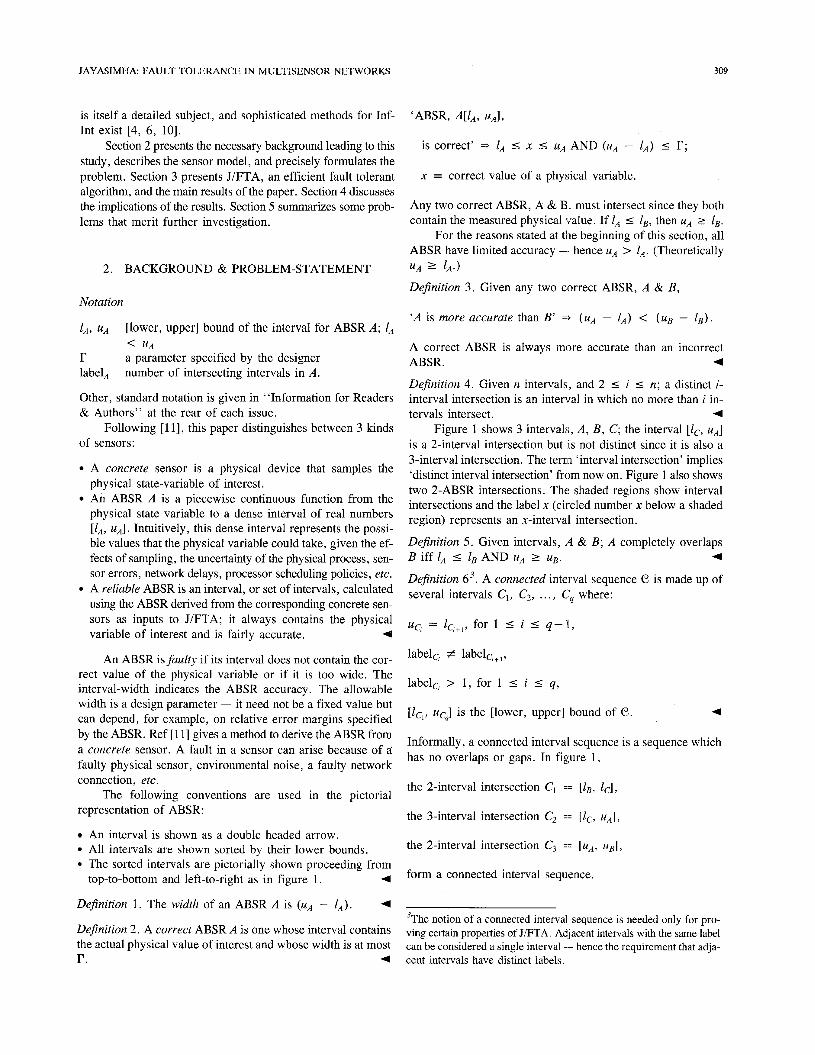
Dejnition 4. Given n intervals, and 2 5 i 5 n; a distinct i- interval intersection is an interval in which no more than i in- tervals intersect. 4

Figure 1 shows 3 intervals, A , B , C; the interval [ I c , UA]

is a 2-interval intersection but is not distinct since it is also a 3-interval intersection. The term ‘interval intersection’ implies ‘distinct interval intersection’ from now on. Figure 1 also shows two 2-ABSR intersections. The shaded regions show interval intersections and the label x (circled number x below a shaded region) represents an x-interval intersection.

Dejinition 5 . Given intervals, A & B ; A completely overlaps

Dejinition 63. A connected interval sequence C is made up of several intervals C1, C2, . . . , C:, where:

B iff LA 5 1B AND U A 1 uB. 4

uc, = I , + , , for 1 I i I 4-1,

labelct # labelc2+, ,

labelc, > I , for 1 I i I q ,

[Ic, , u c - is the [lower, upper] bound of C. 4

Informally, a connected interval sequence is a sequence which has no overlaps or gaps. In figure 1,

the 2-interval intersection C1 == [lB, IC],

the 3-interval intersection C, == [lc, U A ] ,

the 2-interval intersection C, == [U,, uB],

form a connected interval sequence.

3The notion of a connected interval sequence is needed only for pro- ving certain properties of J/FTA. Adjacent intervals with the same label can be considered a single interval -- hence the requirement that adja- cent intervals have distinct labels.

310 IEEE TRANSACTIONS ON RELIABILITY, VOL. 45, NO. 2. I996 JUNE

A

0 0 A , B, C are the 3 ABSR. The label x below a shaded region represents a x-interval intersection.

Figure 1. Pictorial Definitions

Assumptions

1. There are n s-independent ABSR of which no more than fare faulty during the interval of time a measurement is made.

2. There is a synchronization protocol which prevents sen- sor measurements from getting mixed-up.

3. Failures are arbitrary with bounded-inaccuracy [ 111, ie, ‘width of each ABSR’ I r. Iff’ I fsensors have widths more than r, they can be detected as faulty a priori - n & f can both

As shown in section 4, assumption #3 improves the ac- curacy of the output since f/n decreases (improves). The ar- bitrary failure model is the weakest (most general), and includes all other failure models 131. Chew & Marzullo [l] point out the advantage of applying such weak failure models to Inf-Int as opposed to traditional approaches which model a sensor value as a r.v.

be reduced by f’. 4

Observation 1. Any intersection of at least ( n -J) intervals can contain the correct value. Any intersection of less than ( n -J) intervals does not contain the correct value. 4

Thus in figure 1, given that 1 ABSR is faulty, any of the shaded intervals can contain the value of interest. The unshad- ed intervals [ I A , ZB], [uB, uc] do not contain the correct value since they (trivially) form a 1-interval intersection.

This paper constructs a reliable ABSR which is guaranteed to contain the physical value of interest and whose width 5 J?. The reliable ABSR can be constructed as a:

1. Single correct interval of bounded width, or 2. Collection of (n - i)-interval intersections, one of which

contains the correct value. 4

The single correct interval of method #1 is obtained by taking the union6 of all the intervals that arise in #2 and is preferred when the communication requirements need to be kept down

4This assumption is weaker than the usual one: No more than f sen- sors are faulty; once a sensor develops a fault, it remains faulty. 5This assumption #2 might not hold for spatially distributed sensor networks used for time critical applications. For a solution to the syn- chronization problem in such networks, see [8].

or the shape of the ABSR needs to be preserved (for 1-dimensional ABSR, the shape is a line segment). By obser- vation 1, this method of construction yields the reliable ABSR. By taking the union, however, the points in the correct interval which do not belong to any of the possibly correct intervals could be included. The collection of method #2 does not have this problem, and is more accurate than #l. Maintaining the reliable ABSR as a collection of intervals has two advantages:

If this ABSR has to be integrated with others, as in a DSN, the accuracy of the integrated ABSR is better than if the reliable ABSR were a single ABSR. If an ABSR is known to be correct and this information was not available at the time of sampling the physical value, then some interval in the reliable ABSR could be discarded, thereby improving its accuracy. The single correct ABSR of #1 is called the spanning interval.

Dejinition I. The width of a reliable ABSR is the width of its

This work is heavily influenced by [ 111 which provides: spanning interval. 4

a fault-tolerant ABSR averaging algorithm, an algorithm to detect faulty sensors, bounds on the width of the reliable ABSR when f is bounded.

Ref 1111 proves that when:

1. f < gilb( ?h ( n + 1 ) ) , the width of the spanning interval is at least as narrow as one of the sensors;

2. f < gilb(%n), the width is at least as narrow as one of the correct sensors.

Because of our assumption #1, bound #1 is more meaningful. Since each ‘ABSR width’ I r, a consequence of [ l l ] is that the ‘spanning interval produced by J/FTA’ I r.

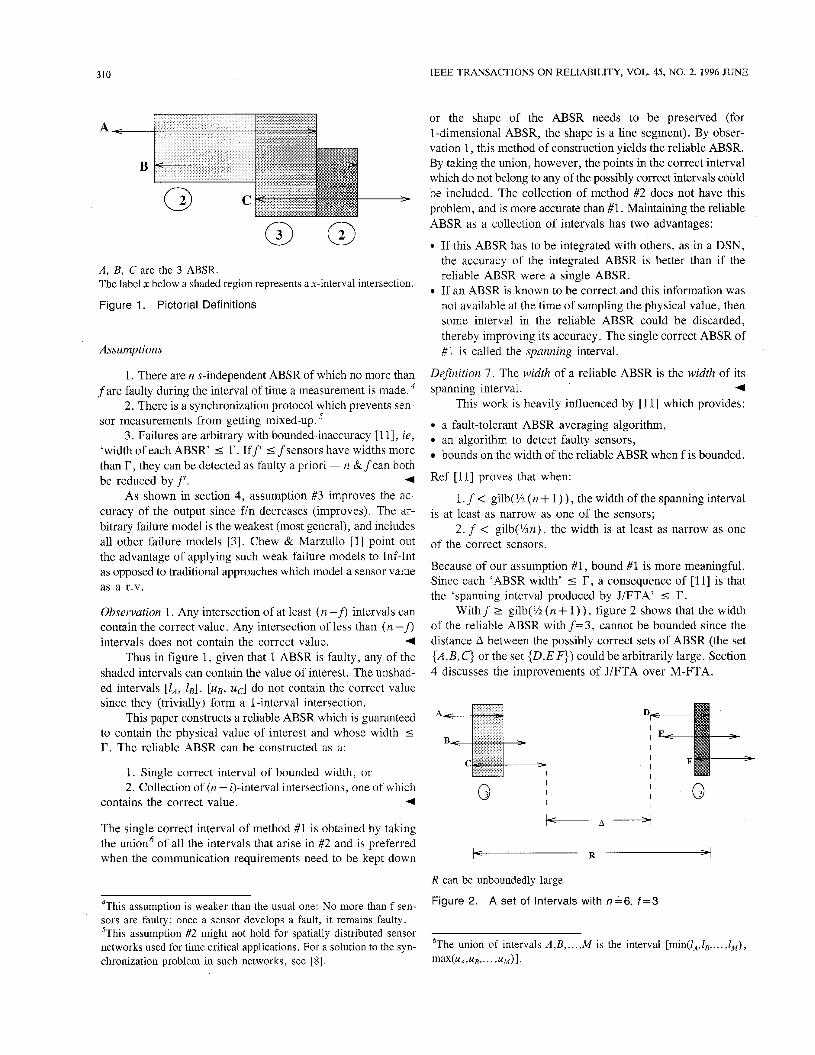
With f 2 gib( ?h ( n + 1 ) ) , figure 2 shows that the width of the reliable ABSR with f = 3, cannot be bounded since the distance A between the possibly correct sets of ABSR (the set {A ,B , C} or the set {D,EF}) could be arbitrarily large. Section 4 discusses the improvements of J/FTA over M-FTA.

I I I

I I I

R can be unboundedly large

Figure 2. A set of Intervals with n-6, f = 3

6The union of intervals A , B ,..., M is the interval [min(Z,,I, ,..., I,), max(uA,uB, ..., uMM)I.

JAYASIMIHA: FAULT TOLERANCE IN MULTISENSOR NETWORKS 311

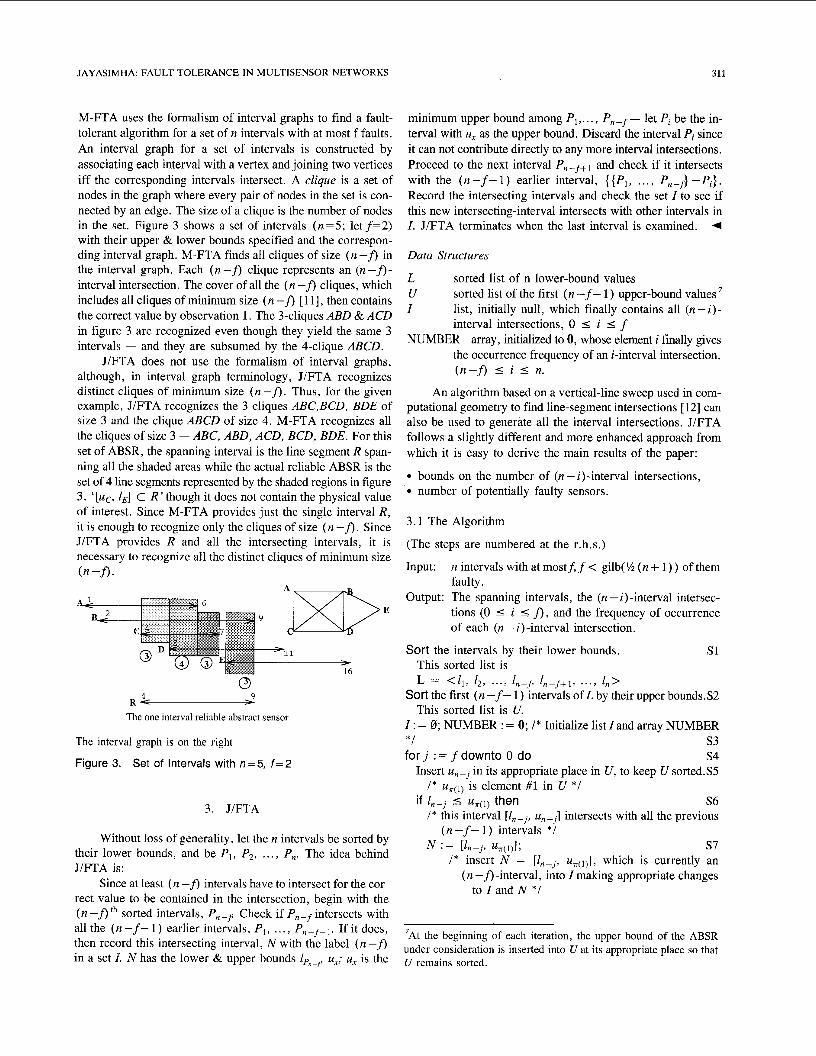
M-FTA uses the formalism of interval graphs to find a fault- tolerant algorithm for a set of n intervals with at most f faults. An interval graph for a set of intervals is constructed by associating each interval with a vertex and joining two vertices iff the corresponding intervals intersect. A clique is a set of nodes in the graph where every pair of nodes in the set is con- nected by an edge. The size of a clique is the number of nodes in the set. Figure 3 shows a set of intervals (n=5; letf=2) with their upper & lower bounds specified and the correspon- ding interval graph. M-FTA finds all cliques of size ( n -J) in the interval graph. Each ( n -J) clique represents an (n -J)- interval intersection. The cover of all the ( n -J) cliques, which includes all cliques of minimum size ( n -J) [ 111, then contains the correct value by observation 1. The 3-cliques ABD & ACD in figure 3 are recognized even though they yield the same 3 intervals - and they are subsumed by the 4-clique ABCD.

J/FTA does not use the formalism of interval graphs, although, in interval graph terminology, J/FTA recognizes distinct cliques of minimum size (n-J). Thus, for the given example, J/FTA recognizes the 3 cliques ABC,BCD, BDE of size 3 and the clique ABCD of size 4. M-FTA recognizes all the cliques of size 3 - ABC, ABD, ACD, BCD, BDE. For this set of ABSR, the spanning interval is the line segment R span- ning all the shaded areas while the actual reliable ABSR is the set of 4 line segments represented by the shaded regions in figure 3. ‘ [uc, LE] C R ’ though it does not contain the physical value of interest. Since M-FTA provides just the single interval R , it is enough to recognize only the cliques of size ( n -J) . Since J/FTA provides R and all the intersecting intervals, it is necessary to recognize all the distinct cliques of minimum size (n-J).

0 9 R %

The one interval reliable abstract sensor

The interval graph is on the right

Figure 3. Set of Intervals with n=5, f=2

3. J/FTA

Without loss of generality, let the n intervals be sorted by their lower bounds, and be P,, P2, ..., P,. The idea behind J/FTA is:

Since at least ( n -J) intervals have to intersect for the cor- rect value to be contained in the intersection, begin with the ( n -J) th sorted intervals, Pn-f Check if Pn-f intersects with all the ( n - f - 1 ) earlier intervals, P1, . . . , Pn-f- ,. If it does, then record this intersecting interval, N with the label ( n -8 in a set I. N has the lower & upper bounds lpn-f, ux; U, is the

minimum upper bound among RI,. . . , Pn-f - let Pi be the in- terval with U, as the upper bound. Discard the interval Pi since it can not contribute directly to any more interval intersections. Proceed to the next interval P,-f+l and check if it intersects with the ( n - f - 1 ) earlier interval, { {P1, . . . , P,-f} -Pi} , Record the intersecting intervals and check the set I to see if this new intersecting-interval intersects with other intervals in I . J/FTA terminates when the last interval is examined. 4

Data Structures

L sorted list of n lower-bound values U sorted list of the first ( n - f - 1 ) upper-bound values I list, initially null, which finally contains all (n - i ) -

interval intersections, 0 5 i I f NUMBER array, initialized to 0, whose element i finally gives

the occurrence frequency of an i-interval intersection, ( n - f ) i i I n.

An algorithm based on a vertical-line sweep used in com- putational geometry to find line-segment intersections [ 121 can also be used to generate all the interval intersections. J/FTA follows a slightly different and more enhanced approach from which it is easy to derive the main results of the paper:

bounds on the number of (n - i)-interval intersections, number of potentially faulty sensors.

3.1 The Algorithm

(The steps are numbered at the r.h.s.)

Input: n intervals with at mostf, f < gilb( ‘/z ( n + 1 ) ) of them faulty.

Output: The spanning intervals, the (n - i)-interval intersec- tions (0 I i I f), and the frequency of occurrence of each (n - i)-interval intersection.

Sort the intervals by their lower bounds.

L = < l l , 12, ...) I n - ) l,-f+1, ..., I n >

s1 This sorted list is

Sort the first ( n - f - 1) intervals of L by their upper bounds.S2

I : = 0; NUMBER : = 0; / * Initialize list I and array NUMBER * / s 3 f o r j := f downto 0 do s 4

Insert U,-] in its appropriate place in U , to keep U sorted.S5 / * u ~ ( ~ ) is element #1 in U * /

if ln-] 5 uT(,) then S6 /* this interval [ I n p J , u,-~] intersects with all the previous

This sorted list is U.

( n - f - 1 ) intervals */ N = [L], uT(1)l; s7

/ * insert N = [ L n p J , u , (~)] , which is currently an ( n -J) -interval, into I making appropriate changes

to I and N * /

7At the beginning of each iteration, the upper bound of the ABSR under consideration is inserted into U at its appropriate place so that U remains sorted.

312 IEEE TRANSACTIONS ON RELIABILITY, VOL. 45, NO. 2, 1996 JUNE

Locate the connected interval sequence C = [C,, C,, . . . , C,] in Z in which each C, intersects with N (lem- ma 1) S8

i f C = 0 s 9 I : = Z U N ; I* N gets added to the tail of I - see lemma

1 * I s10 I* Assign a label and increment the number of ( n -f, -

intervals * I labelN : = n -A S l l a NUMBER[n-fl := NUMBER[n-Jl + 1; S l l b

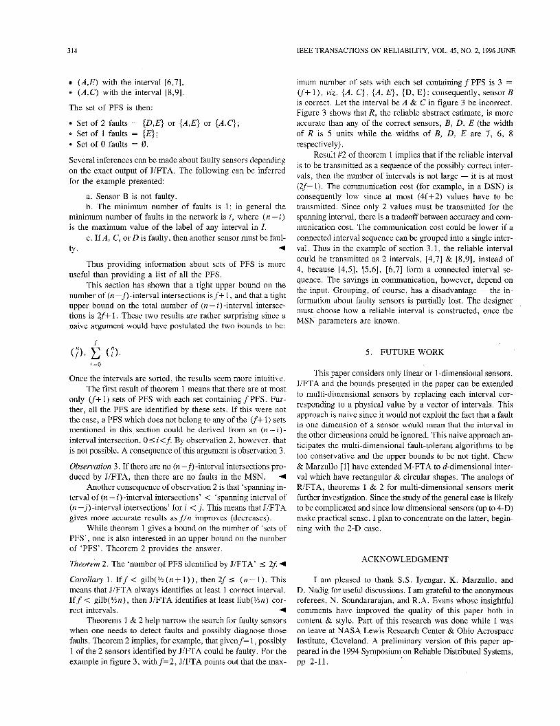
else I* C,, . . . , C, - completely overlaps N , by definition - see theorem 1 * I s12 f o r k := 2 to (p-1) do S13

label, : = label, + 1; S14 NUMBER[labclck] : = NUMBER[labelck] + 1; S15

end-for / * C1 is treated first; then C, *I if lcl = lnp1 then I* C1 completely overlaps with N -

see figure 4a * I S16 labelc, : = labelcl + 1; S17 NUMBER[labelc,] : = NUMBER[labelcl] + 1 ; S 18

else / * IC, < la-] - split [l,,, uc,] into two intervals - see figure 4b *I N I := [IC,, 4-J; labelNi := labelc,; S19 N2 := [ Z n P j , uc,]; labelN2 := labelc, + 1; S20 NUMBER[labelN2] : = NUMBER[label,] + 1; S21 I := (Z U NI U NZ) - C,; s22

end-if if U*(,) < ucp then I* split [Ic-, ucJ into two intervals - see figure 4c * I S23 N3 := [Icp, u,(~)]; labelN3 := labelcp + 1; S24 N4 := [u,(1), uc,]; label, := labelcp; S25 NUMBER[labelN,] : = NUMBER[label,,] + 1; S26

JIFTA has a complexity of 8 ( n .log ( n ) ) because of the sorting in steps S1 & S2.

Theorem 1 shows that the maximum size of Z is (2 f + 1). The search, step S 5 , and locate, step S8, operations can be done efficiently in O(log(n) ) and 0(logv) ) times respectively by maintaining U & I as balanced binary trees [2]. Further, by theorem 1, the loop, steps S13 - S15, is executed at most (2f + 1) times. So the complexity of the main loop is 0 (f- log(n) ).

Iff is small enough (a constant, for example) I could be maintained by a simpler data structure such as a linked list - the locate, step S8, then takes 0 0 time.

Now examine how JIFTA calculates the reliable ABSR for the example in figure 3. For each iteration, the initial & final values of lists L, U, I and the interval N are shown.

Iteration

init. L = <1, 2, 4, 5, 8 > ; U = <6, 9 > ; Z = 0 2 Consider the interval formed by element ( n -31 of L:

[4,71. U = <6, 7, 9 > ; N = (4,6) I = <[4, 61 (3)> L = < 2 , 4 , 5 , 8 > ; U = < 7 , 9 > Consider the interval formed by element ( n - f+ 1 ) of L:

U = <7, 9, 1 1 > ; N = (5,7)

L = < 2 , 5 , 8 > ; U = <9, 11> Consider the interval formed by the last element of L: [8,101. U = <9 , 11, 1 6 > ; N = (8,9)

L = < 5 , 8 > ; U = <11, 16>

1 [5,111.

= < [4, 51 (31, 15, 61 (4), [6, 71 (3) >

0

= <[4, 51 (31, [ 5 , 61 ( 4 ~ 16, 71 (31, [8, 91 ( 3 ~

I := ( I U N3 U N4) - Cp; s27

labelcp : = labelcp + 1; S28a NUMBER[labelcJ : = NUMBER[labelcp) + 1;S28b if uc, < u,(~) then I* create a new (n-fl-interval -

JIFTA terminates at this point. I contains the reliable ABSR intervals. The single interval ABSR is just the lower & upper bounds of I , [4,9]. The frequency of occurrence of 3-, 4-, and 5-interval intersections is (respectively):

else I* ucp 5 u?r(l) - see figures 4d & 4e * I

&e figure 4e * / S29 s30 NUMBER[3] = 3,

Z : = Z U N,; I* N5 gets added to the tail of Z *IS3 1 labelN : = n - j S32a NUMBER[4] = 1,

end-if NUMBER[S] = 0.

N5 : = b C P j u*(l)I;

NUMBER[n-fl := NUMBER[n-fl + 1; S32b

end-if end-if I* remove the interval [1,(1), u,(~)] from the list of ABSR

s33

3.2 Number of Intersecting Intervals

*I Lemma 1. Let: L := L - {Z,,,,}; U := U -

en d f o r the last connected interval sequence appearing in the sorted /* Zgives the multiple ABSR; the lower & upper bounds list Of be = x 2 ~ ...’ xr];

ofZgive the single interval ABSR; NUMBER[i] gives * N = [Ln-j, u?r(1)1> step s7, if it exists, be the interval to be

the frequency of occurrence of an i-interval intersec- inserted into tion. *I

stop Then Z n P j 2 I*,.

Lemma 1 implies that we need to check for the intersec- tion of N only with the last connected interval sequence in I . Complexity of J/FTA

JAYASIMHA: FAULT TOLERANCE IN MULTISENSOR NETWORKS 313

In fact, we choose only the set of intervals in the last connected interval sequence which intersects with N - this is how the con- nected interval sequence C is formed, step S8.

Consider iteration #1, j =f. At the start of this iteration, I=0. During this iteration, if lnPf I u,(~), then [ln-+ un-f1 in- tersects with all the previous ( n -f- 1 ) intervals and forms a

Theorem 1. The number of (n - i) -interval intersections in a set of ri intervals, with at mostfof them faulty, is 5 (2f + 1 ) . me number of ( n -J) -interval intersections in a set of n intervals, with at most f of them faulty8, is 5 cf+ 1). 4

CP< I > cpF cp _I

N N d N-

I I I I I I I I I

(C) (a (e)

Figure 4. Pertaining to Theorem 1

The importance of theorem 1 is discussed in section 4.

new ( n - f , intersecting interval, N (step S7). C=O since I = 0 (steps S3, S9). At the end of the iteration, I = [Z,-f, un-f] if lnPf I u,(~); I = 0 otherwise. Hence P is true, with j=$

Consider each iteration, j , f < j I 0, and let 1, -f I U, ( ).

N is formed appropriately as before, step S7. N can intersect with only the last connected interval sequence in I as shown by lemma 1. Further, as theorem 1 and figure 4 show, all the ways in which N intersects with the last connected interval se- quence in I are considered in (steps S9 - S1 1) and the various subcases of steps S12 - S32. The discussion in the proof of theorem 1 shows that the intersection of N with I could result in a new (n - f , -interval intersection, or in the label of an in- terval in I getting incrementedl by 1.

> u,(~) , at least one interval [1,(1), u,(~)] does not intersect with the current interval [lnPj, unPj] . By lemma 1, neither does [1,(1), u,(~)] intersect with any other interval in I.

The interval [1,(11, u,(~)] can now be discarded, step S33, since any new intersecting interval that could be formed subse- quently has a lower-bound > u,(~).

By the construction outlined here, I has an ( n -J) -interval at the end of iterationf, and the label of an interval in I can be incremented by 1 by the end of each succeeding iteration,

If

in the worst case. Hence I consists of only ( n - i ) , j I i ~ f , in- tersecting intervals considering the first ( n - j ) intervals. P is therefore true. Since it has already been shown that the loop terminates with . j=O, the correctness of J/FTA immediately

Observation 2. By construction, any (n - i) -interval intersec- tion (0 :% i <J) is obtained from the intersection of an (n -J) - interval intersection, and one or more Pi (label 1) intervals.+

3.3 Proof of Correctness

J/FTA computes the set I which consists only of all the (n - i) -interval intersections (0 I i I J) . Since at least ( n -J) intervals have to intersect for the correct value to be contained in the intersecting interval, J/FTA begins with a sorted list (sorted by lower bounds) of ( n - f - 1 ) intervals (steps S1, S2). The I (which is initially empty, step S3) consists only of all the (n-i)-interval (0 I i 5 J) intersections at termination. Predicate P characterizes the main loop, steps S4 - S33:

P: I = (9: q is an (n- i ) , j I i I f, intersecting interval

among the first ( n - j ) intervals}.

P is true after the execution of each iteration of the loop (after step S32). Z, n, J j in P have the same meaning as in J/FTA. After the loop terminates, ie, j = O ) , P asserts that I consists only of all the (n - i)-interval intersections, as desired.

At the beginning of each iteration j (step S4: j takes values f, f- 1, . . ., 0 successively), interval [ln-j, unPj] is examined with ( n - f - 1 ) previous intervals; at the end of each iteration, one chosen interval is discarded, step S33. Hence all the inter- vals are examined and J/FTA terminates.

~ _ _ _ _ _

?his part of the theorem has been proved for the special case of f= 1, in [7] . Theorems 1 & 2 are proved by following the steps of the algorithm.

follows from P, with j = O .

4. DISCUSSION

Two improvements of J/FTA over M-FTA, and the im- portance of the bounds derived in theorem 1 are discussed. A bound on the number of PFS identified by J/FTA is derived using theorem 1.

Improvement #1 concerns the fault tolerant algorithm; J/FTA provides a single interval, as M-FTA does, but, in ad- dition, provides all the (n - i)-interval (0 I i I J) intersec- tions without sacrificing efficiency. Both algorithms have a run- time complexity of 0 ( n .log(n) ) and the run-time constants are comparable.

Improvement #2 concerns fault detection. M-FTA could fail to detect some faulty sensors since it detects only those sen- sors whose intervals do not intersect the spanning interval, as faulty. Thus in figure 3, M-FTA would not detect any sensor as faulty though there is at least one that is (since there is no 5-interval intersection). J/FTA not only detects all the PFS but also all the sets (combinations) of PFS. This can be achieved by associating each interval in I with a set of PFS - sensors whose intervals are not part (sub-interval) of the interval in I. Consider figure 3 - one could associate the set of faulty sensors,

(D ,E) with the interval [4,5;], E with the interval [5,6],

314 IEEE TRANSACTIONS ON RELIABILITY, VOL. 45, NO. 2, 1996 JUNE

( A , E ) with the interval [6,7], 0 ( A , C ) with the interval [8,9].

The set of PFS is then:

Set of 2 faults = {D,E} or {A ,E} or { A , C } ; * Set of 1 faults = { E ) ; * Set of 0 faults = 0.

Several inferences can be made about faulty sensors depending on the exact output of J/FTA. The following can be inferred for the example presented:

a. Sensor B is not faulty. b. The minimum number of faults is 1; in general the

minimum number of faults in the network is i , where ( n - i) is the maximum value of the label of any interval in I .

c. If A , C, or D is faulty, then another sensor must be faul- tY. 4

Thus providing information about sets of PFS is more useful than providing a list of all the PFS.

This section has shown that a tight upper bound on the number of (n -B-interval intersections isf+ 1, and that a tight upper bound on the total number of (n - i) -interval intersec- tions is 2f+ 1. These two results are rather surprising since a naive argument would have postulated the two bounds to be:

f

i = O

Once the intervals are sorted, the results seem more intuitive. The first result of theorem 1 means that there are at most

only (f+ 1) sets of PFS with each set containing f PFS. Fur- ther, all the PFS are identified by these sets. If this were not the case, a PFS which does not belong to any of the cf+ 1) sets mentioned in this section could be derived from an (n - i ) - interval intersection, 0 5 i < f . By observation 2, however, that is not possible. A consequence of this argument is observation 3.

Observation 3. If there are no (n -a -interval intersections pro- duced by J/FTA, then there are no faults in the MSN. 4

Another consequence of observation 2 is that ‘spanning in- terval of (n - i)-interval intersections’ < ‘spanning interval of (n -j)-interval intersections’ for i < j . This means that J/FTA gives more accurate results as f / n improves (decreases).

While theorem 1 gives a bound on the number of ‘sets of PFS’, one is also interested in an upper bound on the number of ‘PFS’. Theorem 2 provides the answer.

Theorem 2. The ‘number of PFS identified by J/FTA’ I 2 $ 4

Corollary 1. I f f < g i l b ( % ( n + l ) ) , then2f1 (n-1). This means that J/FTA always identifies at least 1 correct interval. Iff < gilb(%n), then J/FTA identifies at least liub(%n) cor- rect intervals. 4

Theorems 1 & 2 help narrow the search for faulty sensors when one needs to detect faults and possibly diagnose those faults. Theorem 2 implies, for example, that givenf= 1, possibly 1 of the 2 sensors identified by J/FTA could be faulty. For the example in figure 3, withf=2, J/FTA points out that the max-

imum number of sets with each set containing f PFS is 3 = cf+ l ) , viz, {A , C } , {A , E } , {D, E}; consequently, sensor B is correct. Let the interval be A & C in figure 3 be incorrect. Figure 3 shows that R , the reliable abstract estimate, is more accurate than any of the correct sensors, B, D, E (the width of R is 5 units while the widths of B, D, E are 7 , 6, 8 respectively).

Result #2 of theorem 1 implies that if the reliable interval is to be transmitted as a sequence of the possibly correct inter- vals, then the number of intervals is not large - it is at most (2f+1). The communication cost (for example, in a DSN) is consequently low since at most (4f f2) values have to be transmitted. Since only 2 values must be transmitted for the spanning interval, there is a tradeoff between accuracy and com- munication cost. The communication cost could be lower if a connected interval sequence can be grouped into a single inter- val. Thus in the example of section 3.1, the reliable interval could be transmitted as 2 intervals, [4,7] & [8,9], instead of 4, because [4,5], [5,6] , [6,7] form a connected interval se- quence. The savings in communication, however, depend on the input. Grouping, of course, has a disadvantage - the in- formation about faulty sensors is partially lost. The designer must choose how a reliable interval is constructed, once the MSN parameters are known.

5. FUTUREWORK

This paper considers only linear or 1-dimensional sensors. JiFTA and the bounds presented in the paper can be extended to multi-dimensional sensors by replacing each interval cor- responding to a physical value by a vector of intervals. This approach is naive since it would not exploit the fact that a fault in one dimension of a sensor would mean that the interval in the other dimensions could be ignored. This naive approach an- ticipates the multi-dimensional fault-tolerant algorithms to be too conservative and the upper bounds to be not tight. Chew & Marzullo [ 11 have extended M-FTA to &dimensional inter- val which have rectangular & circular shapes. The analogs of RIFTA, theorems 1 & 2 for multi-dimensional sensors merit further investigation. Since the study of the general case is likely to be complicated and since low dimensional sensors (up to 4-D) make practical sense, I plan to concentrate on the latter, begin- ning with the 2-D case.

ACKNOWLEDGMENT

I am pleased to thank S.S. Iyengar, K. Marzullo, and D. Nadig for useful discussions. I am grateful to the anonymous referees, N. Soundararajan, and R.A. Evans whose insightful comments have improved the quality of this paper both in content & style. Part of this research was done while I was on leave at NASA Lewis Research Center & Ohio Aerospace Institute, Cleveland. A preliminary version of this paper ap- peared in the 1994 Symposium on Reliable Distributed Systems, pp 2-11.

320 IEEE TRANSACTIONS ON RELIABILITY, VOL. 45, NO. 2, 1996 JUNE

Figures 7 & 8 illustrate the results. MTUO tends to in- crease as Bm increases. If the failure rates of multiple separated S-SW, hs2 & hs4, become much smaller than hSl, the MTUO becomes better. System reliability can be appreciably improv- ed by adding 1 spare S-SW to these three types of S-SW. Figure 9 (corresponding to figure 7) shows the result.

ACKNOWLEDGMENT

This study was supported in part by Satellite Technology Research Center at KAIST and by the Korea Science & Engineering Foundation.

REFERENCES

G.B. Alaria, P. Pestefanis, G. Guaschino, et al , “On-board processor for a TSTISS-TDMA telecommunications system”, ESA J . , vol9, 1985, pp 29-37. L. Palmer, L. White, “Demand assignment in the ACTS LBR system”, ICC ’88, 1988, pp 504-509. S.I. Sayegh, F.T. Assal, T. Inuka, “On-board processing architectures and technology”, IEEE EASON, 1988; Arlington. C.W. Wong, “Device technology and baseband switch for the advanc- ed on-board processing satellite”, PhD Dissertation, 1988 Aug; Dept. Electrical & Electronic Eng’g, Univ. of Surrey, Guilford. M.D. Beaudry, “Performance-related reliability measures for computing system”, IEEE Trans. Computers, vol C-27, 1978 Jun, pp 540-547. “Reliability performance objectives for LATA switching system (LSSGR)”, TA-TSY-000512, section 12, 1988 Oct; Bellcore. A. Goyal, A.N. Tantawi, “Evaluation of performability for degradable computer systems”, IEEE Trans. Computers, vol C-36, 1987 Jun, pp 738-744. J.F. Meyer, “On evaluating the performability of degradable computing systems”, IEEE Trans. Computers, vol C-29, 1978 Aug, pp 720-731. R. Huslende, “A combined evaluation of performance and reliability for degradable systems”, Pegormance Evaluation Review, vol 10, num 3, 1981, pp 157-164.

[ 101 R. Billinton, R.N. Allan, Reliability Evaluation of Engineering System: Concepts and Techniques, 1085; Pitman.

[11] K.W. Lee, er al, “Trafficability and reliability analysis for the digital switching network”, Microelectronics & Reliability, vol 28, 1988, pp 263-272.

AUTHORS

Sang H. Kang; Dep’t of EE; KAIST; 373-1, Kusong-dong Yusong-gu; Taejon 305-701 KOREA. Internet (e-mail): shkang@concerto.kaist.ac.kr

Sang H. Kang was born in Seoul, Korea, on 1967 Jun 30. He received the BS (1990) and MS (1992) in Electrical Engineering from Korea Advanced Institute of Science & Technology (KAIST). He is working towards the PhD in Electrical Engineering at KAIST. His research interests include traffic engineering in B-ISDN, performance & reliability of switching systems, and applications of neural networks to switching systems.

Min Y, Chung; Dep’t of EE; KAIST; 373-1, Kusong-dong Yusong-gu; Tae- jon 305-701 KOREA.

Min Y. Chung was born in Taejon, Korea, on 1967 Jan 23. He receiv- ed the BS (1990) and MS (1994) in Electrical Engineering from KAIST. He is working towards the PhD in Electrical Engineering at KAIST. His research interests include performance & reliability evaluation of switching systems and intelligent networks.

Prof. Dan K. Sung; Dep’t of EE; KAIST; 373-1, Kusong-dong Yusong-gu; Taejon 305-701 KOREA. Internet (e-mail) : dksung@eekaist . kaist . ac. kr

Dan K. Sung received the BS (1975) in Electrical Engineering from Seoul National University, and the MS (1982) and PhD (1986) in Electrical & Com- puter Engineering from the University of Texas at Austin. From 1977 May to 1980 July, he was a research engineer with the Electronics & Telecommunica- tions Research Institute. In 1986 he joined the faculty of the Korea Institute of Technology and is now Associate Professor of Dept. of Electrical Engineering at KAIST. His research interests include ISDN switching systems, ATM swit- ching systems, wireless networks, and performance & reliability of systems. He is a member of IEEE, KITE, KICS, and KISS.

Manuscript received 1995 November 2

Publisher Item Identifier S 0018-9529(96)05732-6 4 T R F

Fault Tolerance in Multisensor Networks

(continued from page 3 15)

AUTHOR Professor at the Department of Computer & Information Science, The Ohio State University, Columbus. He was a Visiting Senior Research Associate at

Dr, D. N. Jayasimha; Dep,t of Computer Information Science; 395 Dreese Lab; The Ohio state University; 2015 Neil Ave; Columbus, Ohio 43210 USA. Internet (e-mail): iavasim@cis.ohio-state.edu

the NASA Lewis Research Center Cleveland during 1993-94. His research in- terests are in parallel computing, computer architecture, and distributed-sensor networks. He is a member of the ACM, IEEE, and The Society of Sigma Xi. - . -

D. N. Jayasimha (M) received the BE in Electronics Engineering from the University Visvesvaraya College of Engineering, Bangalore; the ME in Com- puter Science from the Indian Institute of Science, Bangalore, and the PhD in Computer Science from the University of Illinois, Urbana. He is an Assistant

received 1996 lo

Publisher Item Identifier S 0018-9529(96)05635-7 4 T R b