FB SubmitCSR08-06 Part1 - Swansea University

12345efghi

UNIVERSITY OF WALES SWANSEA

REPORT SERIES

Alternative subcell discretisations for viscoelastic flow: Part I

by

F. Belblidia, H. Matallah, B. Puangkird and M. F. Webster

Report # CSR 8-2006

F.Belblidia et al. Alternative subcell discretisations for viscoelastic flow: Part I (CSR-08-2006) Page 1 of 52


F. Belblidia, H. Matallah, B. Puangkird and M. F. Webster†

Institute of non-Newtonian Fluid Mechanics, Department of Computer Science, Digital Technium, Swansea University, Singleton Park, Swansea, SA2 8PP, UK.

Abstract

This study is concerned with the investigation of the associated properties of subcell

discretisations for viscoelastic flows, where aspects of compatibility of solution function spaces are

paramount. We introduce one new scheme, through a subcell finite element approximation fe(sc), and

compare and contrast this against two precursor schemes – one with finite element discretisation in

common, but at the parent element level quad-fe; the other, at the subcell level appealing to hybrid

finite element/finite volume discretisation fe/fv(sc). To conduct our comparative study, we consider

Oldroyd modelling and two classical steady benchmark flow problems to assess issues of numerical

accuracy and stability - cavity flow and contraction flow. We are able to point to specific advantages

of the finite element subcell discretisation and appreciate the characteristic properties of each

discretisation, by analysing stress and flow field structure up to critical states of Weissenberg number.

Findings reveal that the subcell linear approximation for stress within the constitutive equation (either

fe or fv) yields a more stable scheme, than that for its quadratic counterpart (quad-fe), whilst still

maintaining third order accuracy. The more compatible form of stress interpolation within the

momentum equation is found to be via the subcell elements under fe(sc); yet, this makes no difference

under fe/fv(sc). Furthermore, improvements in solution representation are gathered through enhanced

upwinding forms, which may be coupled to stability gains with strain-rate stabilisation.

Keywords: high-order pressure-correction, viscoelastic, stability, subcell approximations, upwinding.

† Corresponding author. Tel: +44 1792 295656; fax: +44 1792 295708; Email: [email protected]


1. Introduction

Here, we are interested in analysing subcell discretisations for viscoelastic flows. In this regard, we

are motivated by our earlier work, where we constructed a hybrid finite element/finite volume (fe/fv)

pressure-correction formulation, utilising triangular parent finite elements for velocity-pressure

coupling and subcell approximation for stress, of cell-vertex finite volume form (akin to linear fe

interpolation). The advantages of such a combination are now well established in the viscoelastic

literature, inclusive of incompressible [1-5] and mildly-compressible flow settings [6-8]. We point to

the dual issues raised here: a) parent element and function spaces versus parent-child elements and

their associated function spaces; b) finite element versus finite volume discretisation and associated

constructs. Under the former aspect and the finite element domain, there have been related

contributions from Marchal and Crochet [9] and Basombrio et al. [10], which have both pointed to the

superior system compatibility properties that might be attracted by linear stress interpolation (see also

Baaijens [11] for discontinuous stress treatment), in the presence of quadratic velocity representation.

Marchal and Crochet [9] also had recourse to introduce fe-subcell approximation (stress), but over

rectangular elements. The selection of order/continuity and treatment of velocity gradients is a

strongly interconnected issue, handled in various means: global Galerkin and localised recovery are

two such, where we opt here for the latter, directing the reader to focused work on this particular topic

itself (in Part II of this study).

In the light of this knowledge, we wish to identify the properties of a new subcell finite element

fe(sc)-approximation, which essentially replaces the fv-subcell form within our hybrid finite fe/fv(sc)

pressure-correction system. This fe(sc)-scheme can be characterised against both the pure finite

element discretisation at the parent element level, quad-fe, and the hybrid subcell scheme, fe/fv(sc) –

so, via three individual schemes. To conduct our comparative study, bearing in mind established

benchmark data, we consider the Oldroyd-B model viscoelastic fluid and two classical steady-state

problems: cavity flow and abrupt-corner contraction flow. Both problems are treated within a plane

Cartesian frame-of-reference. The cavity flow is an entirely enclosed predominantly-shear flow,

comprising of closed streamlines, the motion being sustained by a continuous parabolic lid-driven

velocity profile. This problem is particularly useful to categorise orders of mesh convergence across

schemes. In contrast, the contraction flow is a non-smooth flow with inflow-outflow boundaries,

manifesting a mixture of shear and extensional deformation. This problem poses a severe singularity

in stress and velocity gradient at the sharp re-entrant corner, disclosing such solution features as lip-

vortices and downstream stress boundary layers in sub-critical to critical Weissenberg number (We)


solution fields. The response of the various schemes proposed, in their ability to tightly capture such

solution features, is a common measure adopted to report on their relative stability properties.

Throughout the study aspects of compatibility of solution function spaces are paramount. This

arises through the subcell formulation itself for stress, and through its consequences, via secondary

variables such as velocity gradients, and associated terms in the momentum equations. These issues

lie in common upon each of the three schemes proposed. So, for example, this discloses one form of

momentum stress-term representation based upon quadratic parent-elements, Quad-τMom. An

alternative, is to adopt the subcell functions, yielding the Lin-τMom implementation. There is also the

distinction to draw between finite element and finite volume upwinding constructs and variations

therein, placing this within the context of the above study. Of particular relevance here is the use of

“Streamline Upwind Petrov Galerkin (SUPG)” for fe-schemes and “Fluctuation Distribution” stencils

for fv-schemes. The former may be augmented with a cross-stream diffusion treatment via

Discontinuity Capturing (DC) [11-13]; the latter provides us with “Low-Diffusion-B (LDB)” stencils,

that are advanced to “Positive Streamwise Invariance (PSI)” forms. In addition, stabilisation

techniques [8,14-16] may be applied to all scheme variants to enhance robustness, under which we

consider one form of “Strain-Rate-Stabilisation (SRS)”– akin to DEVSS formulations [15].

We are able to point to specific advantages of the fe(sc)-discretisation and appreciate the

characteristic properties of each discretisation in turn, by analysing stress and flow field structure up

to critical states of Weissenberg number. We find it particularly useful to refer to the work of Alves et

al. [17], Oliveira and Pinho [18] and Aboubacar et al. [3-5] on vortex behaviour – suppression of

salient-corner vortices and emergence of separate lip-vortices. Stress boundary layers (see Renardy

[19]) appear in field plots and are commented upon as and when relevant.

In our recent work [8] and elsewhere [14-16], SRS-inclusion has provided the most improvement

in levels of critical We reached, while stress-peak levels have been constrained. Theoretically, the

appended term in the SRS-formulation has the dual effect of controlling cross-stream solution

propagation and meeting compatibility requirements between function spaces on stress and velocity

gradients, a la extended LBB-condition satisfaction. In addition, the SRS-term, which is spatially

localised at the re-entrant corner, was found to characterise convergence patterns in the temporal

error-norm for stress. As such, one may attribute the considerable elevation of Wecrit under SRS to the

tight capturing of the stress singularity and its resulting downstream boundary layer, accordingly.

Under the issue of compatibility of function spaces, the specific role that stress/velocity-gradient

interpolation plays is a key aspect. In the present study to avoid subjugation and over-complication,

we adopt a single approximation for velocity-gradient representation, that of localised


superconvergent recovered form [20], continuous and quadratic on the parent fe-triangular element.

We place this approach alongside alternative global/local approaches in a companion study, Part II,

where we can do justice to this detailed matter. In Table I, we categorised variable interpolation

selection and definition with regards to these fe/fv(sc) and fe(sc) schemes.

2. Governing equations and finite element analysis

The non-dimensional governing equations for an isothermal, viscoelastic, incompressible fluid

flow of densityρ may be represented in the form of conservation of mass and transport of

momentum, supplemented by a constitutive equation for stress. These equations of momentum, mass

and extra-stress may be expressed for the Oldroyd-B model:

pt

∇−∇⋅−+⋅∇=∂∂

uuDu

Re)2(Re 2 ττττµ , (1)

0=⋅∇ u , (2)

))((2 T1 uuuD ∇⋅−∇⋅−∇⋅−−=

∂∂ ττττττττττττττττττττ

Wet

We µ , (3)

where ττττ and p u, represent the velocity, pressure, and extra-stress, respectively. Total stress may be

segregated into viscous and elastic parts, ττττ+= DT 22µ , and the rate-of-deformation tensor is

defined through the velocity gradients, u∇=TL , as: ( ) 2TLL +=D . Here, the zero shear viscosity

is divided into polymeric ( )1µ and viscous ( )2µ contributions, so that 210 µµµ += . In addition, we

introduce the dimensionless Reynolds (Re) and Weissenberg group numbers (We), as 0Re µρ lU=

and lUWe λ= .

The resulting space-time discrete matrix-vector system extracted from the fe-semi-implicit Taylor-

Galerkin/pressure-correction scheme may be expanded in the following form [21]:

Stage 1a

( ) ( ) ( ) 112

2

12 )](Re[)(

2

Re2 −+−++−++−=−

++∆

nnnTnSRS

nn

SRS PPPLBNSSSSMt

θµµTUUUU

nnn

NNWeWeNMMMt

We))()(())((2)(

2 T1

2

1

LLUD ΤΤΤΤΤΤΤΤΤΤΤΤΤΤΤΤΤΤΤΤ +++−=−∆

+µ

Stage 1b

( ) ( ) ( ) 112

1

22 )](Re[)(

2

Re −+ −++−++−=−

++∆

nnnTnSRS

nSRS PPPLBNSSSSM

tθµµ

TUUUU*


2

1T

11 ))()(())((2)(

++ +++−=−∆

nnn LNNWeWeNMMMt

We ΤΤΤΤΤΤΤΤΤΤΤΤΤΤΤΤΤΤΤΤ LUDµ (4)

Stage 2

*ULt

PPK nn

∆=−+

θRe

)( 1 (5)

Stage 3 )()(Re 1* nnT PPLM

t−−=−

∆++ θUU 1n . (6)

Here, the superscript (n) denotes the time level, t∆ the time-step, 21=θ and 10 1 ≤≤ θ . Precise

matrix forms are provided below, once spatial discretisation has been introduced.

The SRS-term appended to the momentum equation, see Eq.(4) in Stage 1a and 1b, is evaluated

as: ( ) ( ) Ω−⋅∇∫Ω dDDn

ci 22µαφ , over the domain Ω with quadratic weighting functions( )xiφ . In this

approach, the appended stabilisation term within the momentum equation takes the form of the

difference between the discontinuous rate-of-deformation (D ) under fe-approximation, and its

recovered equivalent (cD ), based on localised velocity gradient recovery procedures [20]. An optimal

α -parameter setting, scaling (22µ ), is found empirically in [8] to be 21 µµα= . Further details on

SRS methodology procedures employed are provided in [8].

2.1 Quadratic and subcell finite-element methodology

Here, the quadratic-fe (parent) grid may be utilised as a platform for the subcell (sc) grid, from

which control domains are constructed. Each cell is composed of four sub-triangles, formed by

connecting the mid-side nodes of the parent element, as illustrated in Figure 1. Stress variables are

located at the vertices of the cells, which renders direct interpolation on either parent or subcell

elements. Originally, under the parent quadratic-fe scheme, the stress was approximated through

quadratic shape functions )(xjφ , whilst under fe(sc) representation, linear stress interpolation

)(xkψ is employed. Independent of scheme employed, we also appeal to a recovery-type technique

(see Matallah et al. [20]) to enhance the quality of velocity gradient representation. Interpolation of

variable fields is concisely provided through notation as (see Table I),

∑=

=6

1

,),(j

jjt Uxu φ ,),(3

1∑

=

=k

kk Ptp ψx and

=

∑

∑

=

=

3

1

6

1

(sc)

(par)

),(

kkk

jjj

t

T

T

x

ψ

φττττ . (7)


Based on such interpolation on a single elemental/subcell fluid area dΩ, we define the matrix

notation of Eqs. (4-6). For the diffusion (S), the pressure stiffness (K) and the L and B matrices,

conventional parent (par) element representation of [6,22] is employed. Alternatively across

equations, for the consistent mass (M) and the advection (N) matrices, the following generalised

definitions emerge, appealing also to the subcell (sc):

Ω

Ω

Ω

=

∫

∫

∫

Ω

Ω

Ω

sc

scjsci

jpar

i

ji

ij

d

d

d

M

sc)-(stress

par)-(stress

par)-(mom.

ψω

φω

φφ

,

Ω∇

Ω∇

Ω∇

=

∫

∫

∫

Ω

Ω

Ω

sc

scjllsci

jllpar

i

jllpar

i

ij

d

d

d

N

sc)-(stress)(

par)-(stress)(

par)-(mom.)(

)(

ψφω

φφω

φφφ

U

U

U

U

and

Ω

Ω

=∫

∫

Ω

Ω

sc

scjllsci

jllpar

i

ijd

d

Nsc)-(stress)(

par)-(stress)(

)(ψψω

φφω

T

T

T , and 4/Ω=Ω sc . (8)

In the above, Galerkin weighting may be applied on parent or subcell elements as:

=(sc)

(par)

i

ii ψ

φω

2.1a) Streamline Upwinding Petrov-Galerkin (SUPG): Conventional Galerkin fe-discretisation is

ideal for the approximation of diffusion-based problems, as they are optimal for self-adjoint (elliptic)

problems (see [20]). This applies for the equations of motion (continuity and momentum) in the low

Reynolds number regime where they display elliptic-dominated character. In contrast, the Oldroyd-B

constitutive equation displays hyperbolic character. For its effective numerical discretisation, it is

necessary to employ some form of upwinding treatment. In this regard, the SUPG-variant has been

successfully employed to stabilise the Galerkin formulation for convection-dominated flows, see for

example [23]. Here, it is employed as a base for the quadratic-fe and fe(sc) schemes. The SUPG-

weighting function is defined as:

∇⋅+

∇⋅+=

(sc)

(par)

ih

i

ih

ii

ψαψφαφ

ωu

u, (9)

where, u is the velocity vector and hα is a scalar SUPG-parameter [13]. hα is a function of mesh

size, unit velocity vector ( )kj vv , and local coordinates ( )iξ , over parent element or subcell, so that,


≥

≤≤∆=

1 if 1

10 if 2

gg

ggthα with kj

k

i

j

i vvxx

g∂∂

∂∂

=ξξ

. (10)

2.1b) Discontinuity capturing (DC): The Discontinuity Capturing (DC) stabilisation technique is

grafted on to the SUPG-scheme described above. Without lose of generality, focus is given to the

fe(sc) implementation. Under the DC-scheme, a term is appended to SUPG-weighting function to act

in the solution gradient direction. This has the effect of stabilising the scheme and smoothing the

solution field, thereby capturing strong discontinuities in a local and compact manner [14]. The

weighting function (10) is supplemented to:

ih

ih

ii ψβψαψω ∇⋅+∇⋅+= puu . (11)

Here, hhh τττ ∇⋅

∇∇⋅=

2uu p is the projected velocity in the stress-gradient direction,

hβ is the DC-parameter (defined below) and hτ is the elemental stress solution. Conventionally, this

amendment would be applied in weighting to all terms of the constitutive equation. Shakib [13] also

proposed an alternative DC-implementation, pragmatically instigated via a single-term inclusion.

Carew et al. [12] and Matallah et al. [14] have employed this approach on the parent element and

found that it provided superior stability properties over the form of Eq.(11). This second approach is

preferred here implemented on the subcell, with the following term appended to the discretised

constitutive equation:

Ω∇⋅∇∫ dhi

h τψβ ξξ . (12)

Following the Shakib [13] implementation, [ ]T321 ,,, ξξξξ ∂∂∂∂∂∂=∇ I . As ( )iψ are linear order

functions, hence ( ) [ ]T,,, IIIIi =∇ ψξ , where I is identity operator. The parameter hβ is provided

in [13], see also Baajens [11], as:

2

22

h

h

h

τ

τβ

ξ∇

ℑ= , (13)

where, the residual of the interpolated constitutive equation hτℑ is defined as:

,2 hhhh ταττα

ℑ⋅ℑ=ℑ and ,2 hhh τττ ξξξ ∇⋅∇=∇ with: hα the SUPG-parameter of Eq.(10).

To ensure uniform boundness of the hβ factor of less than unity, Carew et al. [12] incorporated the

safeguard:


>

≤=

2for 2

2for 222

22

bssb

bsbsh

hh

α

αβ with hh bs ττ ∇=ℑ= , . (14)

In contrast to the fe(sc) method with DC-stabilisation, below we turn our attention to the hybrid-

fe/fv(sc) variant with its improved stabilised form.

2.2 Hybrid finite-element/volume methodology

As for the fe(sc) scheme described above, the hybrid fe/fv(sc) scheme enjoys improved quality of

recovered velocity. Wapperom and Webster [2] employed a quadratic Galerkin fe-formulation for the

equations of motion and a fv-form for the constitutive equation alone, namely: hybrid-fe/fv(sc). This

has some similarity with the 4x4 stress sub-elements of Marchal and Crochet [9]. Here, a Fluctuation

Distribution (FD) upwinding technique is applied to stress equation that distributes control volume

residuals and compute nodal solution updates. Briefly, the constitutive equation is divided into a

convective flux and source terms. The treatment applied to these terms leads to different upwinding

strategies, object of the current study. The reader is referred to references [3,8,24] for extensive

details on the hybrid fe/fv(sc)-formulation.

The integration of Esq.(3) for each scalar component of stress tensor,ττττ , on an arbitrary volume

provides the time, flux( )R and source( )Q residuals:

∫∫∫ ΩΩΩΩ+Ω=Ω

∂∂

Tl

Tl

Tl

dQdRdt ˆˆˆ

ττττ, (15)

where, flux ττττ∇⋅= uR and source ( ) T1 )(2

1uuD ∇⋅+∇⋅+−= ττττττττττττµ

WeQ .

The core of this cell-vertex FD-scheme is to evaluate these flux and source terms on each fv-

triangle. In the above expression, integrals can be evaluated over different control volumes, namely:

the subcell triangle T and/or median-dual-cell (MDCT) control volume (l) (see Figure 1a). The update

for a given node (l) is obtained by summing the contributions from control volume, lΩ , that is

composed of all fv-triangles surrounding node l, as illustrated in Figure 1a. Furthermore, the stability

of this approach was improved further [2,24,25] by adding to it the MDC contribution and taking their

proportional weight (see [24]) as:

( ) ( ) ( )21

1

ˆˆ Ω

++

Ω

+=

∆− ∑∑ ∀∀

+T

lMDC

lMDCMDCT TT

TlT

nl

nl TTT

QRQR

t

δαδττττττττ , (16)

where, depending on definition of areas 1Ω and 2Ω , we retrieve a class of schemes: (CTi, i=1,3),

introduced in [24]. The parameters Tδ and MDCδ , with TMDC δδ −= 1 , are applied to discriminate


between various update strategies, being functions of fluid elasticity, We, velocity field, a, and mesh

size, h. Parameter Tδ may be chosen from two alternative forms [24], either

≥

<=

3 if 1

3 if 3

ξξξ

δT with ( )haWe=ξ , (17)

or ( )TT

TT QR

R

+=δ . (18)

For the latest CT3-scheme, introduced in [24], which was found the most adequate in tracking

transient solutions, areas weighting factors are set as MDCFD Ω+Ω≡Ω=Ω ˆˆˆˆ21 , where

∑ Ω=ΩlT T

TlTFD αδˆ and ∑ Ω=Ω

l TMDC TMDCMDC δˆ , with TΩ defined as the area of triangle T.

There is a natural decay of Tδ in form (18) from unity to zero through the hyperbolic function

employed without a need for truncation and being independent of mesh size. Seeking consistency for

comparison with earlier work, we have selected form (17).

We proceed to introduce the various FD-schemes of fe/fv(sc)-construct analysed in this study,

namely LDB and PSI. For more detail on these upwinding schemes, the reader is referred to the

background literature [26-29]. These schemes are constructed to observe the numerical properties of

conservation ( )1=∑lT

Tlα on any given triangle cell T, and linearity preservation, to represent the

steady-state solutions exactly for linear problems. Positivity, which relates to the flux term, implies

the preservation of monotonocity by prohibiting the emergence of new extrema in the solution. In

fact, positivity is a convenient but non-necessary criterion for developing non-oscillatory solutions, by

bounding each i-nodal solution component at time-step (n+1) in terms of local max-min from the

previous time-step (n).

2.2a) Low Diffusion B (LDB) scheme: The LDB-scheme is found to be appropriate, for steady

viscoelastic flows [5,24] where source terms may dominate. This is a linear scheme with linearly

preservation and non-positive properties and second-order accuracy [5]. It conveys a relatively low-

level of numerical diffusion in comparison to a linear positive scheme [2]. The LDB-distribution

coefficients iα are obtained on each triangle via angles 21,γγ (defined in Figure 1b), subtended at an

inflow vertex (i) by the advection velocity a (average of velocity field per fv-triangular cell), viz.


( )21

21

sin

cossin

γγγγα

+=i , ( )21

12

sin

cossin

γγγγα

+=j and 0=kα . (19)

Note, there is no dependence between the LDB-delivery factors and the magnitude of the advection

velocity. We also observe that when 1γ is larger than 2γ , then iα is larger than jα , and hence by

design, node (i) gains a larger flux contribution than node (j). Interestingly, the closer a is to being

parallel to one of the boundary element sides, the larger is the contribution to that downstream

boundary node.

2.2b) Positive Streamwise Invariant (PSI) scheme: The PSI-scheme is positive and linearly

preserving scheme. Satisfying both properties, it must be a non-linear scheme. It has invariance

towards direction within a triangle and is first-order accurate in time and second-order accurate at

steady-state. It is equivalent to the Narrow N-scheme with a minmod limiter [27], which is a linear

positive β-scheme. The scheme has shock-capturing capabilities and has the lowest cross-diffusion

noise. We note, the positivity property demands special care when source terms are included [30]. By

first defining the N-scheme coefficients as:

( )kιii k ττττττττ −−=β and ( )kιjj k ττττττττ −−=β , (20)

we may establish PSI-distribution coefficients, iα , determined to satisfy conditions:

>==

<==<+

jiii

jiii

jiββαα

ββααββ

for0,1

for1,0then0 ,

21then0 ===+ jiji ααββ ,

( ) ( )jijjjiiiji βββαβββαββ +=+=>+ andthen0 . (21)

3. Flow problems

In the present study, we introduce two benchmark problems based on an Oldroyd-B fluid to

evaluate subcell schemes characteristics with regard to stability and precision, namely a lid-driven

cavity flow and a sharp 4:1 plane contraction flow. The lid-driven cavity flow problem is mainly

applied for the computations of viscous flows [22,31-33]. In the viscoelastic context, this problem

presents singularities at both lid corners [34]. Recently, Fattal and Kupferman [35,36] introduced a

log-conformation representation to address the highly elastic solutions for the Oldroyd-B model, a

key issue in developing their new scheme. It is known that stress experiences a combination of

deformation and convection giving rise to steep exponential stress profiles. These spatial profiles are

poorly approximated by numerical schemes based on polynomial interpolations (as with finite


element and finite difference forms). This often results in an imbalance between the rate of

deformation and convection contributions, providing a source of instability for constitutive models of

Oldroyd-B type. Fattal and Kupferman [35,36] scaled the stress field logarithmically, which should

remain strictly positive. This is achieved by appealing to the conformation tensor, a positive-definite

(SPD) quantity, directly related to stress. Their novel implementation was found to be stable even at

large We, with results presented for the cavity problem up to We=5.0 in [36], although scheme

accuracy degraded with insufficient mesh resolution (see other critical assessment, Afonso et al.

[37]). The focus of the present work is different: instead we are concerned with compatibility

arguments through stress interpolation order and element reference.

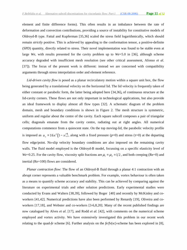
Lid-driven cavity flow is posed as a planar recirculatory motion within a square unit box, the flow

being generated by a translational velocity on the horizontal lid. The lid velocity is frequently taken of

either constant or parabolic form, the latter being adopted here [34,36], of continuous structure at the

lid-cavity corners. These flows are not only important in technological applications, but also provide

an ideal framework to display almost all flow types [32]. A schematic diagram of the problem

domain, mesh and boundary conditions is shown in Figure 2. The mesh structure is symmetric,

uniform and regular about the centre of the cavity. Each square subcell composes a pair of triangular

cells; diagonals emanate from the cavity centre, radiating out at right angles. All numerical

computations commence from a quiescent state. On the top moving-lid, the parabolic velocity profile

is imposed as ( )2216 1xu x x= − , along with a fixed pressure (p=0) and stress (τ=0) at the departing

flow edge/point. No-slip velocity boundary conditions are also imposed on the remaining cavity

walls. The fluid model employed is the Oldroyd-B model, focussing on a specific elasticity level of

We=0.25. For the cavity flow, viscosity split fractions are 2121 == µµ , and both creeping (Re=0) and

inertial (Re=100) flows are considered.

Planar contraction flow: The flow of an Oldroyd-B fluid through a planar 4:1 contraction with an

abrupt corner represents a valuable benchmark problem. For example, vortex behaviour is often taken

as a means to quantify scheme accuracy and stability. This can be achieved by comparing against the

literature on experimental trials and other solution predictions. Early experimental studies were

conducted by Evans and Walters [38,39], followed by Boger [40] and recently by McKinley and co-

workers [41,42]. Numerical predictions have also been performed by Renardy [19], Oliveira and co-

workers [17,18], and Webster and co-workers [3-6,8,20]. Many of the recent published findings are

now catalogued by Alves et al. [17], and Rodd et al. [42], with comments on the numerical scheme

employed and vortex activity. We have extensively investigated this problem in our recent work

relating to the quad-fe scheme [6]. Further analysis on the fe/fv(sc)-scheme has been explored in [8],


where different stabilisation methods were introduced and contrasted against the basic fe/fv(sc)

scheme (LDB). Here, the numerical stability of the fe(sc) scheme is thoroughly investigated. A

schematic representation of the domain with boundary conditions is depicted in Figure 3a. We take

advantage of flow symmetry about the horizontal central axis of the problem. Various meshes (M1,

M2, M3), illustrated in Figure 3b, have been employed in an extensive mesh refinement analysis

under quad-fe and fe/fv(sc). This has appeared in past published articles [3,5,6] where accuracy and

mesh convergence were established. Here, we extend the scope to the fe(sc) scheme also. The total

length of the planar channel is 76.5 units. A characteristic velocity is chosen as the downstream

channel mean-velocity, whilst the half-channel width L is taken as the characteristic length. We

consider creeping flow (Re=0) for the Oldroyd-B model, with viscosity fractions of 981 =µ and

912 =µ . No-slip boundary conditions are assumed on the solid boundary. At the inlet, transient

boundary conditions of Waters and King [43] type are imposed, through a set of transient profiles for

normal velocity (Ux) and stress (τxx, τxy), and vanishing cross-sectional component (Uy) and stress

(τyy). In contrast, at the domain exit, a zero-pressure reference level is imposed with vanishing (Uy).

Furthermore, at domain exit, natural boundary conditions are established through boundary integrals

and consistent momentum equation representation. At the first non-zero We-solution stage, (i.e.

We=0.1) simulations commence from a quiescent initial state in all variables. Subsequently, a

continuation strategy in We is employed in steps of say 1.0=∆We , until the numerical scheme fails

(diverges or oscillates).

4. Results and discussion

We begin by considering the cavity flow, the quad-fe and the subcell schemes, fe(sc) and fe/fv(sc).

Initially only base-form constructs of fe-SUPG and fv-LDB are considered.

4.1 Cavity flow: convergence and solution

Under the cavity flow problem, three numerical schemes are investigated: quad-fe (or simply fe in

figures), and both fe(sc), and fe/fv(sc). Oldroyd-B steady-state solutions are extracted for each scheme

at We=0.25 starting from quiescent conditions. Particular attention is paid to mesh accuracy for spatial

and temporal convergence trends, variable fields through contour, profile and stream-function plots. A

principal point of comparison is to demonstrate the impact of inertia for such flows.

4.1a) Spatial convergence: Due to the lack of an analytical solution in the viscoelastic context, a fine

mesh solution on 80x80 is taken as a reference, against which two further mesh solutions are


compared (20x20 and 40x40). In this paper, a spatial order of convergence is computed by evaluating

the root mean square error norm( )2hE in its departure from the 80x80 mesh solution.

Third order is achieved for all numerical schemes tested for both stress and velocity, as shown in

Figure 4 and reported in Table II. Nevertheless, the quad-fe scheme offers the highest rate of

convergence for both velocity (about 3.6) and stress (about 3.1). On the other hand, quad-fe is the

slowest in time convergence, as more time steps are required to reach a steady-state solution to a

preordered tolerance (say O(10-7)). For the subcell-variants, the fe/fv(sc) approximation has an order

of convergence in velocity higher than that for the fe(sc) scheme. However, this position is reversed

under trends in stress. There is a consistent shift in error norm plots for velocity between quadratic

and linear interpolation types. Nonetheless, there is no shift or gain in rate of convergence for stress.

For this particular problem, we also observe larger error norm magnitude of one order for τxx above

other components.

4.1b) Temporal convergence: Assessment of temporal-convergence trends to steady-state has been

performed based on creeping flow considerations and under the finest mesh (80×80) square sub-

divisions. Such trends under individual solution components of velocity, stress, and pressure variables

under the three numerical schemes are depicted in Figure 5a. As shown, convergence to steady state is

largely governed by stress, independent of scheme employed, reflecting a superior rate of

convergence for all solution components under linear stress interpolations in contrast to their

quadratic counterpart. Less time-steps are required in velocity development under the fe(sc)

approximation to reach an equitable level of tolerance, followed by that of the fe/fv(sc) variant. Stress

temporal convergence increments for different mesh distributions and numerical schemes are shown

in Figure 5b. A general observation is that the finest mesh distribution demands less time (iteration)

steps than for the coarser mesh partition. Note, independent of mesh-size, the same rate of time-

stepping convergence in stress is observed with both subcell schemes (fe/fv(sc) and fe(sc)).

Oscillations are encountered under fe/fv(sc) with coarser meshing, yet revert to smooth profiles as the

mesh is sufficiently refined. In summary, one may infer that subcell stress interpolations provide

better spatial and temporal rates of convergence in contrast to their quadratic stress interpolation

equivalent.

4.1c) Stream function: Under creeping flow and for the finest mesh solution at We=0.25, stream

function patterns, as depicted in Figure 6, are found insensitive to the numerical scheme employed.

This provides a level of confidence in the validity of solutions for all scheme tested. The streamlines

display the recirculating nature of the flow, with distortion near the singular corners, and a secondary


Moffatt-type vortex in the lower right-corner. The results with inertia inclusion (Re=100) are

contrasted against the inertia-less case (Re=0) in Figure 6. Streamlines are twisted and distorted with

increase of inertia (Re) towards the downstream corner, and the primary vortex centre drops within

the cavity, following trends as in Fattal and Kupferman [36]).

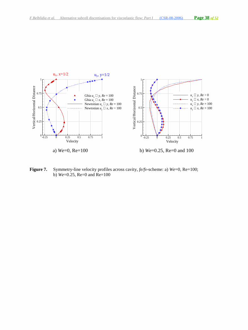
In Figure 7, we illustrate profile plots of velocity components (ux, uy) across the cavity central lines

(x=1/2, y=1/2), under Newtonian on the left (We=0, Re=100), and viscoelastic on the right (We=0.25,

with and without inertia effect). Note, that the purely viscous results for any of the three schemes

match closely those observed by Ghia et al. [31]. Under the viscoelastic context, the vertical velocity

component (uy) is symmetric, and the change of sign in the horizontal component (ux) occurs at the

same position independent of inertial considerations. As under We=0, we barely observe any

differences between solutions for the three alternative scheme approximations, and therefore, only the

fe/fv-scheme findings are presented here.

4.1d) Field variables: Validation is sought for the numerical schemes under investigation, being

conducted for Re=0 and Re=100. Figure 8, illustrates variables fields. Stress component contours

exhibit steep gradients only in the vicinity of the upper lid. The τxx-component has a thin boundary

layer along the lid, and all three components have large gradients near the upper corners. The contour

patterns for the three numerical schemes replicate each other. Nevertheless, there are localised

differences in τ-maxima at peak points, and hence are reproduced for the fe/fv-scheme only. Figure 8

also shows the shift in the flow pattern as inertia increases. Note, profile plots for velocity

components across the cavity central lines, along with streamlines and stress fields at We=0.25, follow

the solution trends reported by Fattal and Kupferman [36] under We=1.0, 2.0 and 3.0 at Re=0.

On the lid, the velocity is constrained as a boundary condition, whilst pressure, τxy and τyy reveal

the same patterns under the three numerical approximations. However, quad-fe offers the largest peak

value in τxx, larger than for fe(sc) and fe/fv(sc); precisely, peaks at x = 0.38 are 30.3, 29.7, and 28.5,

respectively. Independent of scheme employed, the position of the peak-level differs between stress

components. It is positioned upstream of the lid-centre for τxx, and in the far downstream, just before

the corner, for both τxy and τyy. Fattal and Kupferman [36] stated that for Newtonian fluids, the

discontinuity of the flow field at the upper corners causes the pressure to diverge, without affecting

the well-posedness of the system. A viscoelastic fluid cannot sustain deformation at a stagnation

point, therefore the motion of the lid needs to be regularized such that u∇ vanishes at the corners.


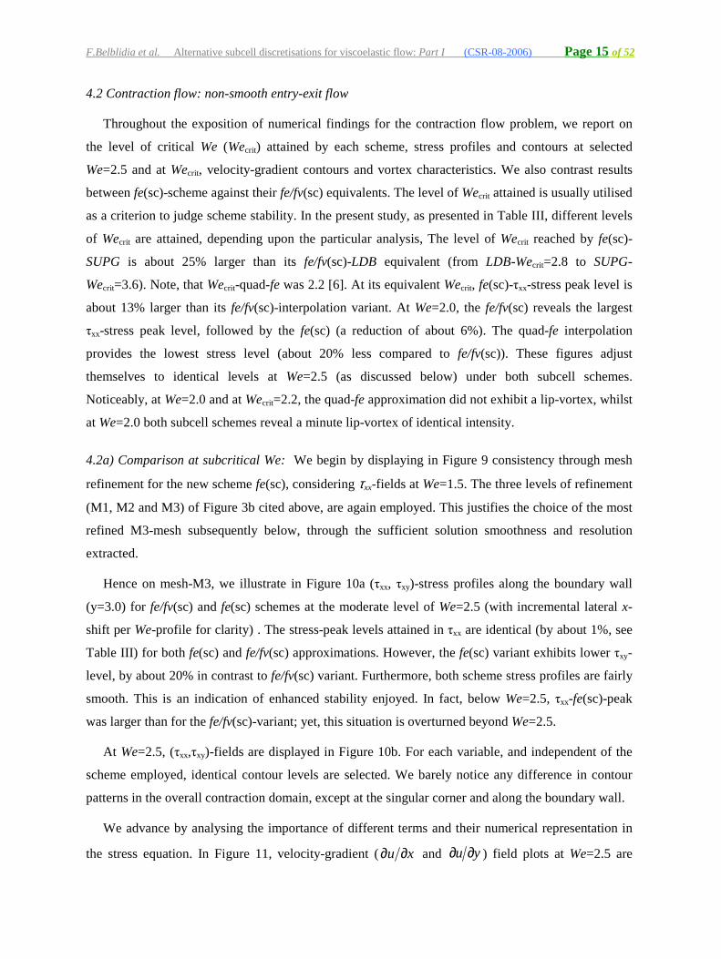
4.2 Contraction flow: non-smooth entry-exit flow

Throughout the exposition of numerical findings for the contraction flow problem, we report on

the level of critical We (Wecrit) attained by each scheme, stress profiles and contours at selected

We=2.5 and at Wecrit, velocity-gradient contours and vortex characteristics. We also contrast results

between fe(sc)-scheme against their fe/fv(sc) equivalents. The level of Wecrit attained is usually utilised

as a criterion to judge scheme stability. In the present study, as presented in Table III, different levels

of Wecrit are attained, depending upon the particular analysis, The level of Wecrit reached by fe(sc)-

SUPG is about 25% larger than its fe/fv(sc)-LDB equivalent (from LDB-Wecrit=2.8 to SUPG-

Wecrit=3.6). Note, that Wecrit-quad-fe was 2.2 [6]. At its equivalent Wecrit, fe(sc)-τxx-stress peak level is

about 13% larger than its fe/fv(sc)-interpolation variant. At We=2.0, the fe/fv(sc) reveals the largest

τxx-stress peak level, followed by the fe(sc) (a reduction of about 6%). The quad-fe interpolation

provides the lowest stress level (about 20% less compared to fe/fv(sc)). These figures adjust

themselves to identical levels at We=2.5 (as discussed below) under both subcell schemes.

Noticeably, at We=2.0 and at Wecrit=2.2, the quad-fe approximation did not exhibit a lip-vortex, whilst

at We=2.0 both subcell schemes reveal a minute lip-vortex of identical intensity.

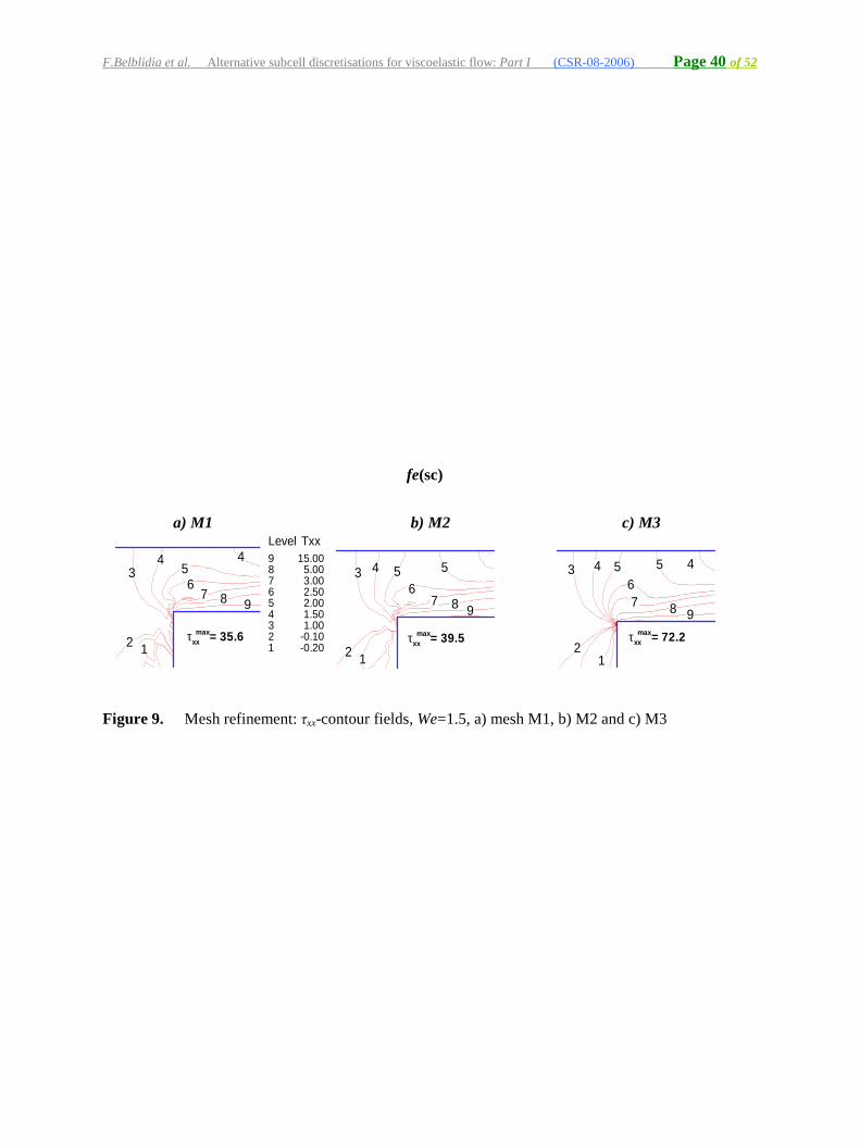
4.2a) Comparison at subcritical We: We begin by displaying in Figure 9 consistency through mesh

refinement for the new scheme fe(sc), considering τxx-fields at We=1.5. The three levels of refinement

(M1, M2 and M3) of Figure 3b cited above, are again employed. This justifies the choice of the most

refined M3-mesh subsequently below, through the sufficient solution smoothness and resolution

extracted.

Hence on mesh-M3, we illustrate in Figure 10a (τxx, τxy)-stress profiles along the boundary wall

(y=3.0) for fe/fv(sc) and fe(sc) schemes at the moderate level of We=2.5 (with incremental lateral x-

shift per We-profile for clarity) . The stress-peak levels attained in τxx are identical (by about 1%, see

Table III) for both fe(sc) and fe/fv(sc) approximations. However, the fe(sc) variant exhibits lower τxy-

level, by about 20% in contrast to fe/fv(sc) variant. Furthermore, both scheme stress profiles are fairly

smooth. This is an indication of enhanced stability enjoyed. In fact, below We=2.5, τxx-fe(sc)-peak

was larger than for the fe/fv(sc)-variant; yet, this situation is overturned beyond We=2.5.

At We=2.5, (τxx,τxy)-fields are displayed in Figure 10b. For each variable, and independent of the

scheme employed, identical contour levels are selected. We barely notice any difference in contour

patterns in the overall contraction domain, except at the singular corner and along the boundary wall.

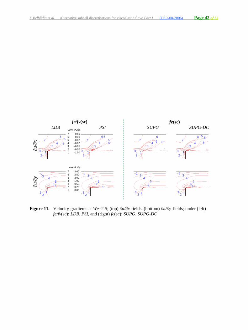
We advance by analysing the importance of different terms and their numerical representation in

the stress equation. In Figure 11, velocity-gradient ( xu ∂∂ and yu ∂∂ ) field plots at We=2.5 are


presented for both stress interpolations. This illustrates the largest and most active velocity gradient

component is yu ∂∂ , being present in both τxx and τxy-equations, and therefore strongly influences

the stress fields. We observe numerical noise in xu ∂∂ (streamwise gradient), particularly under

fe/fv(sc) interpolation, whilst yu ∂∂ (transverse gradient) remains relatively smooth. Note that, at the

lower level of We=2.0, corresponding contours remain smooth.

4.2b) Solutions with increasing We: τxx-stress profiles with increasing We are displayed in Figure 12

for both fe/fv(sc) and fe(sc) stress interpolations. These profiles are smooth up to the level of Wecrit for

both schemes. The fe(sc) approximation is found to be more stable as it reaches a larger Wecrit=3.6

(an increase of about 25% in contrast to fe/fv(sc), Wecrit=2.8) and maintains profile smoothness. Under

fe/fv(sc) interpolation, the τxx-stress profile remains fairly smooth after the re-entrant corner at

Wecrit=2.8. In contrast, under the fe(sc)-scheme, at Wecrit=3.6, the τxx-profile presents a highly

localised second dip, just downstream of the re-entrant corner, absent at the We=3.0 level (unattained

with fe/fv(sc)). The location of this dip coincides with the change in mesh density observed at x=24

(see Figure 3b). The containment of these oscillations is thought to be responsible for subsequent

scheme stability at this We-level. (τxx,τxy)-fields are displayed in Figure 13 at Wecrit for each scheme

variant. We observe a relative smoothness of fe(sc) and fe/fv(sc) contours at their respective Wecrit.

4.2c) Vortex behaviour: Vortex characteristics and trends provide a reasonable measure of the quality

of the numerical scheme under investigation. For the Oldroyd-B model, we observe a reduction in

salient-corner vortex intensity with increasing elasticity whilst the lip-vortex, when present is

enhanced. Trends in vortex activity, displaying salient-corner vortex size and intensity, and lip-vortex

intensity with increasing We are provided in Figure 14 (top) for both subcell schemes. In Figure 14

(bottom), we contrast streamline plots for both schemes variants at specific We levels (at 1.0, 2.0 and

Wecrit). For the size and intensity of the salient-corner vortex, close agreement is observed amongst

the various schemes considered. Salient-corner vortex response with increasing We is unaffected by

the particular choice of scheme. Furthermore, as shown in Figure 14, the computed results match

those of Alves et al. [17] on a very fine mesh. This adds further credence in the quality of the

generated solutions. Furthermore, both scheme variants display a lip-vortex, which is more intense

under the fe(sc) interpolation, at We=2.0 and beyond, in contrast to that under the fe/fv(sc)

counterpart. This discrepancy is mainly due to the type of upwinding procedure employed within the

constitutive equation for each stress interpolation, being SUPG for fe(sc) and FD for fe/fv(sc) variant

(see below, under discussion on the analysis of different upwinding methodologies employed).


From our previous work [7] on quad-fe and fe/fv(sc) schemes, we have observed that lip-vortex

appearance is delayed with quad-fe in contrast to fe/fv(sc). See Table III, where at We=2.0, there is an

apparent lip-vortex for both subcell schemes, whilst up to Wecrit=2.2 there is none present for the basic

quad fe-scheme. Interestingly at We=1.5, a minute lip-vortex of 0.27*10-4 intensity emerges under

fe(sc) interpolation, equivalent to that extrapolated by Alves et al. [17]. At this We=1.5 level, with

fe/fv(sc) a lip-vortex is still absent. Additionally, we have also demonstrated that inclusion of

compressibility considerations promotes lip-vortex characteristics [8,7], in contrast to under a purely

incompressible flow setting. Furthermore, we have found in previous studies that lip-vortex

characteristics are somewhat sensitive to both the numerical treatment applied to tackle the

singularity, and to the quality of the mesh around the corner. Overall, we have also observed that with

increasing elasticity, there is salient-corner vortex reduction, whilst the lip-vortices grow separately,

without merging even at large We. These observations remain valid under the present study.

5. Supplementary upwinding strategies

The implementation and analysis of two alternative upwinding techniques (PSI and SUPG-DC) are

discussed: the extension of PSI (Positive Streamwise Invariant) to the base-scheme fe/fv(sc) (LDB);

and DC (Discontinuity Capturing) to the base-scheme fe(sc) (SUPG). Here, the PSI-scheme provides

invariance towards direction within a triangle cell, in contrast to LDB-counterpart. The PSI-scheme

has embedded shock-capturing properties, suppressive to cross-stream diffusion. Likewise, SUPG-

DC-scheme has an appended term upon the SUPG-weighting function, which acts in the solution

gradient direction. Theoretically, this has a cross-stream stabilisation influence, smoothing solution

fields by tightly capturing strong discontinuities. Improvement in scheme stability and accuracy is

examined through the study of trends in salient-corner and lip vortex behaviour.

For clarity and consistency, results of this section are contrasted against those for the base-schemes

introduced in section 4.2 above, reintroducing oncemore the figures exposed in the previous section.

A summery of results is presented in Table III, contrasting findings at the various levels of Wecrit

reached, stress peak-levels attained and vortex characteristics derived. There is about 11% reduction

in Wecrit under the fe/fv(sc), from LDB to PSI. Further reduction of about 22% is observed under the

fe(sc), from SUPG to SUPG-DC. Also at We=2.5, there is a reduction of about 10% in stress-peak

level attained for both upwinding schemes in contrast to their base-scheme counterparts.

5.1 Comparison at subcritical We=2.5

We recall stress (τxx,τxy) profile and contour plots illustrated in Figure 10. Identical stress-peak

levels are observed with base-schemes in both stress components. Nonetheless, the application of


additional upwinding constructs has reduced these stress levels by the same amount independent of

the scheme. The reduction is about 9% for τxx and about 6% in τxy. Under the PSI-scheme we have

also observed a larger stress-dip, occurring just downstream of the re-entrant corner. At this We-level,

there is barely any difference in stress fields, except near the corner, tightly to the downstream wall,

where the expansion of level contour 9 for τxx and level contour 7 for τxy in Figure 10 is restrained by

these particular upwinding additions. Similarly at this We-level, the introducing of further upwinding

forms has provided little improvement to respective base schemes on velocity-gradient fields as

clearly illustrated in Figure 11.

5.2 Increasing We

The introduction of upwinding methods has a direct impact on solutions, reducing the level of

Wecrit. This is shown in Figure 12, illustrating τxx-stress profiles along the downstream boundary wall.

Under the fe/fv-PSI-scheme, Wecrit declines from 2.8 (LDB) to 2.5 (PSI). The fall is more pronounced

under the fe-SUPG-DC variant which reduces Wecrit from 3.6 (SUPG) to 2.8 (SUPG-DC).

Nevertheless, stress profiles remain smooth under all schemes. The second-dip in τxx-profile (beyond

the corner), occurring at Wecrit=3.6 under fe-SUPG, remains at the same location (x=24) and is deeper

with fe-SUPG-DC at Wecrit=2.8. Here, DC-inclusion is shown to tightly (locally) capture the

downstream stress boundary layer. We observe that beyond We=2.0, the first-dip level in τxx-profile,

attained just after the re-entrant corner, is negative with fe/fv(sc) and deepens with increasing We. On

the contrary, with fe(sc), first-dip levels remain positive, being practically zero. As depicted in Figure

13, stress fields at respective Wecrit for all schemes, retain smoothness across the domain in both τxx

and τxy components. Notably, the application of these additional upwinding constructs has proven to

be responsible for the control of such stress oscillation, at the expense of some reduction in Wecrit.

5.3 Vortex behaviour

The study of salient-corner vortex characteristics and comparison to published results provides

validation for the schemes employed. Observed vortex characteristics with increasing We are

displayed in Figure 14. Oncemore, close agreement is observed between base-scheme

implementations and their upwinding variants, matching the findings of Alves et al. [17] slightly

better on forms fe(sc)-SUPG-DC and fe/fv(sc)-PSI on size and intensity. Overall, the lip-vortex is

more enhanced under fe(sc) schemes taken in contrast to fe/fv(sc) alternatives. At We=2.0, lip-vortex

intensity with fe/fv-PSI is about half that for fe-SUPG-DC. We observe identical lip-vortex

characteristics at any We under fe(sc), when switching between SUPG and SUPG-DC, noting the

restriction of Wecrit to 2.8 for the latter. In particular, lip-vortex characteristics at selected We for the


PSI-scheme are more elevated than those with the LDB-variant, with the former closely tracking

fe(sc) solutions. This are related to the difference in upwinding strategy employed and somewhat as a

consequence of the nature of the mesh around the lip-vortex zone, as exposed below.

6. Enhancing stability through strain-rate stabilisation (SRS)

In our recent work [8], strain-rate stabilisation (SRS) has been thoroughly investigated under our

base-scheme fe/fv(sc) (LDB). SRS-inclusion has been found to promote the stability of the scheme,

doubling Wecrit from 2.8 to 5.9. Previous findings in [8] have shown that SRS-term contributions were

localised ‘precisely’ about the re-entrant corner, independent of the We-level of the solution.

Temporal convergence trends in the (D-Dc)-variable have replicated those observed in stress. In

addition, the application of the SRS-term lowers stress-peak levels attained for any selected We-

solution, in contrast to the equivalent scheme without SRS, a feature that may be responsible for the

improved stability and further advance in We.

Likewise, in the present context, we analyse SRS-term inclusion on the base subcell schemes, and

fe(sc)-SUPG-DC and fe/fv(sc)-PSI. That is with a view to interrogating enhancement in stability,

without significant degradation in accuracy. Here we consider impact upon salient-corner vortex

characteristics, Wecrit attainment. Findings based on SRS-application are summarised in Table IV,

reporting on critical We and stress-peak levels attained at We=2.5 and Wecrit.

6.1 Stress profiles and fields

In Figure 15, we gather τxx-profiles for SRS-implementations with increasing We, covering fe/fv(sc)

(left: LDB/PSI) and fe(sc) (right: SUPG/SUPG-DC). For the purpose of immediate comparison and

for each scheme in turn, we illustrate graphically the contrast against the non-SRS solution within a

separate window (i). The detailed structure of the SRS-solution around the re-entrant corner is

expanded upon in a second zoomed plot, also in a separate window (ii).

Beginning with fe/fv(sc) and as noted previously, SRS-inclusion has significantly elevated Wecrit for

the LDB-variant from 2.8 to a level of 5.9. In addition, at We=3.0 and beyond, we observe the

emergence of oscillations occurring downstream just after the re-entrant corner. With increasing We,

the region of such oscillations broadens, whilst they increase in amplitude and frequency. We may

argue that this is a natural feature occurring for larger We-solutions at these elevated We-levels; yet, it

is their localisation that is responsible for stability gains (Figure 15a). At We of 2.8 and earlier, no

such oscillations are apparent, with or without SRS-inclusion (see Figure 15a-i). By switching to the

SRS-PSI-alternative, we are able to determine the specific effect that the choice of fluctuation


distribution strategy has upon such issues. Here and in contrast to LDB-solutions, we now see in

Figure 15b that these oscillations are practically removed, right up to Wecrit=4.0. Such perturbations

might be introduced due to lack of grading in mesh near the wall at x=24 for We≥3.0. We note

therefore, the attendant enhancement in stability for this scheme with SRS-inclusion, raising Wecrit

from 2.5 to 4.0, as apparent in the separate window plot. We recognise that comparable levels of

respective Wecrit-stress-peak are reached between these schemes, with SRS-LDB of 157.3 units and

SRS-PSI of 157.4 units, yet the Wecrit differ (WecritSRS-LDB=5.9, Wecrit

SRS-PSI=4.0). At We=2.5 (solid-lines

in Figure 15), the SRS-PSI-stress-peak is about 8% larger than for the SRS-LDB-alternative; the SRS-

LDB-form also has a lower downstream first-dip beyond the corner (see below). At We=4.0, the SRS-

PSI-stress-peak grows to about 51% larger than that equivalently with SRS-LDB. With respect to

stress-dip levels and trends with increasing We, we observe that SRS-LDB-solutions switch from

positive to ever decreasing negative values for solutions, We>3.0 (loss of evolution factor, see below).

Under SRS-PSI, stress-dip levels remain small but positive throughout all We-solutions, which is not

the case under non-SRS implementations for We>2.5. Under LDB, the position is that such negative

values arise at We=2.0 with the non-SRS form (less than with PSI), being delayed in onset under SRS

till We=3.0.

In likewise fashion, SRS-inclusion has improved the stability properties of fe(sc)-variant schemes,

SUPG and SUPG-DC: reaching identical Wecrit=4.3 for both with SRS, as opposed to without, of

SUPG-Wecrit =3.6 and SUPG-DC-Wecrit =2.8. The introduction of DC is subtle: it influences solution

quality with increasing We at larger We-levels, beyond say 2.5 for the current problem. This may be

discerned from trends in stress, through profiles and evolution factor, where we may observe that

there is greater control (tighter capture) with DC than without, particularly apparent upon downstream

oscillations (arising beyond We=4.0 in fe(sc)-variants); this lies in company with suppression of

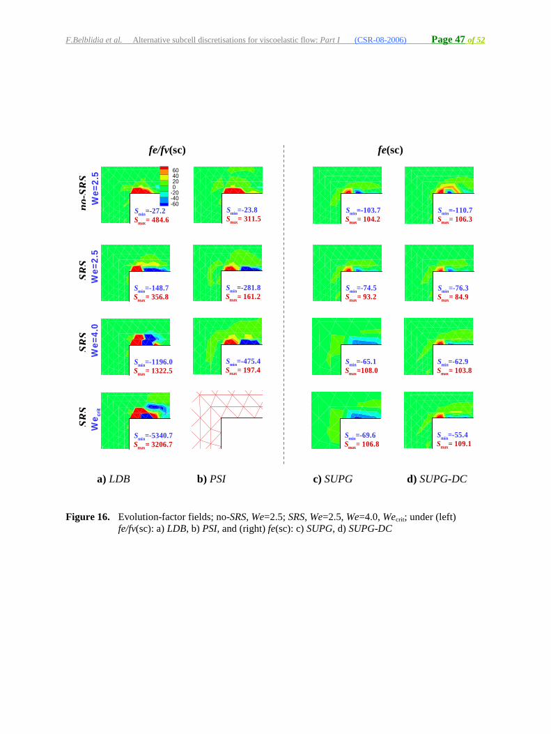
growth in the stress-evolution factor (Figure 16). Conspicuously, stress-peak levels are relatively

independent of DC-inclusion; though we do observe a tendency to plateau out from sub-critical

We=4.0 to critical level of 4.3. If anything, and at the lower level of We=2.5 where SRS has less

impact, SUPG stress-peak level is about 8% larger than with SUPG-DC (not too significant). All first

stress-dip levels are negative beyond We=3.0 for SRS-fe(sc) schemes and prove deeper with DC-

inclusion. Likewise, second reflected stress-peaks are more pronounced with DC then without; clearly

a consequence of more tight solution capture in this area. If SRS-treatment is discarded, such negative

stress-dip levels beyond We=3.0 are much reduced in magnitude over those with inclusion.

At respective Wecrit per upwinding-variant, taking fe/fv(sc) (left) and fe(sc) (right) scheme variants,

we appreciate the penetration into the stress field and the influence of SRS-term inclusion via contours


in Figure 17, contrasted against equivalent non-SRS-solutions of Figure 13. Largely these fields retain

smoothness up to and including their respective Wecrit for each scheme. That is with the exception of

SRS-LDB-solutions, where τxy-contours are non-smooth at the super-elevated level of Wecrit=5.9, this

being introduced first around We=4.5. Fields are smooth and practically identical between SRS-fe(sc)

solutions and SRS-PSI around the comparable levels of We of 4.0 and 4.3; this may not be so under

SRS-LDB, and certainly departs at the super-critical level of Wecrit=5.9.

6.2 Vortex behaviour

We observe that the addition of SRS-treatment upon schemes LDB, PSI, SUPG and SUPG-DC did

not alter prior trends in salient-corner vortex behaviour, which lie in close agreement with Alves et al.

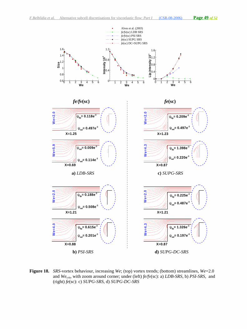
[17], only continuation to larger Wecrit-levels. This trend is charted in Figure 18 (top). In contrast,

SRS-adjustment is observed to have significant impact on near corner solutions, and therefore, on lip-

vortex development as depicted in Figure 18 (bottom). Under SRS-fe(sc) and increasing We, lip-

vortex characteristics are identical up to Wecrit=4.3. Taking variation under fe/fv(sc) schemes, we

observe comparable but slightly lower trends with PSI-form and SRS-fe(sc). The trends are very

different with LDB.

Furthermore, SRS-lip vortex trends are more elevated than those without SRS-adjustment by

around 3 times at We=2.0 for all schemes except for LDB where the difference is much larger (by

about 8 times) (see Figure 14). For fe/fv(sc) schemes, the response under the non-inclusion of the SRS-

term, has been markedly different between LDB and PSI-variants, being considerably more prominent

under PSI (see Figure 14). Likewise, SRS-inclusion has slightly elevated PSI-lip-vortex intensity. It is

conspicuous that SRS-inclusion practically removes the lip-vortex at large We under the LDB-variant,

a position which is examined next.

6.3 Lip-vortex and SRS-LDB

The fact that SRS-adjustment has removed the lip-vortex at larger We under the fe/fv(sc)-LDB-

scheme, whilst under fe/fv(sc)-PSI-SRS, where the lip-vortex is still present at Wecrit=4.0, raises some

questions. Under all other schemes (with or without SRS) we have observed enlargement of lip-vortex

intensity, increasing with increasing elasticity. This remark is in line with findings elsewhere [8,17].

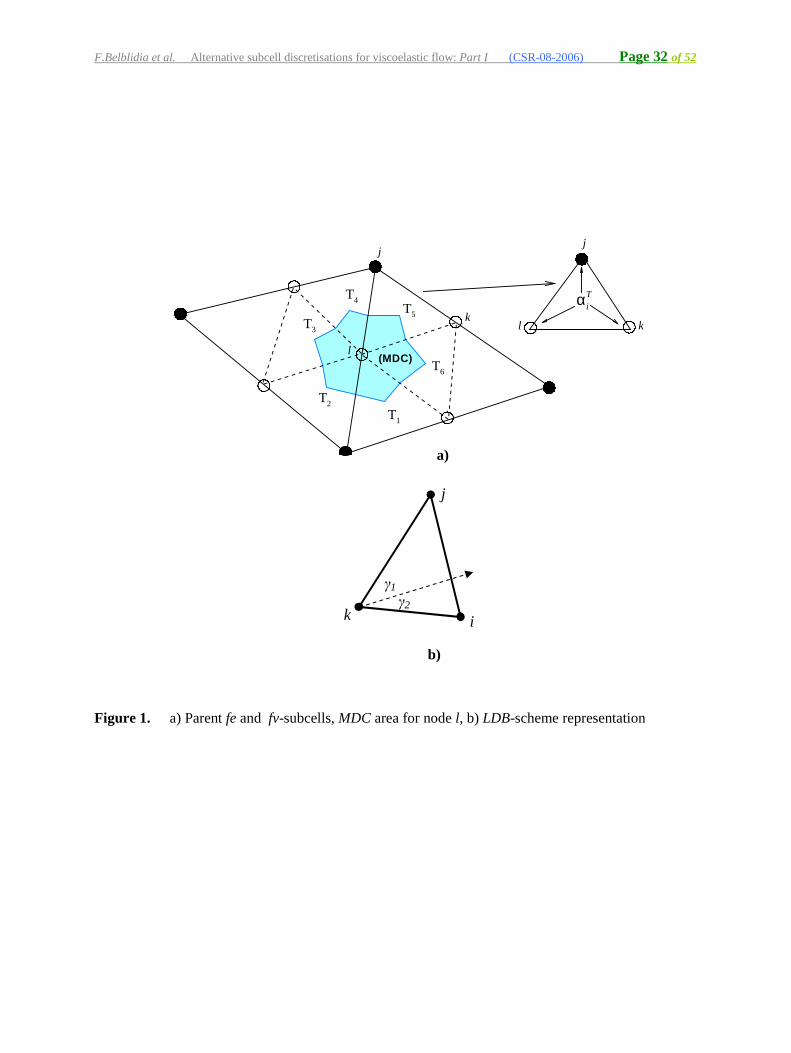
To clarify the position, by design and for the LDB-scheme, the closer the advection velocity is to

being parallel to an element boundary, the larger the contribution to the downstream boundary node

(combine Figure 1b and Eq.(19)). A scrutiny of the mesh orientation in the lip-vortex vicinity (Figure

19-i)) reveals some element sides are parallel to the boundary wall just before the corner; this spurns

velocity-advection vectors (a) parallel to this wall. Consequently, the LDB-upwinding parameter


evaluates to 02 =γ , and thus, 0== kj αα and 1=iα (Figure 1b). Hence, all contributions are delivered

to the upstream node, leaving no possibility for a lip-vortex to emerge. To quantify this position, a

modified mesh has been generated (Figure 19-ii)), by repositioning the set of nodes across the corner

zone so that 02 ≠γ , as shown in Figure 19 (zoomed). Under this mesh adjustment and for both LDB

and SRS-LDB schemes, a lip-vortex now appears, as consistent with other findings. This indicates

again, the sensitivity of the numerical solution to the precise discretisation of the corner problem.

With regard to system residual (mass-loss), locations where this concentrates remain localised around

the corner, independent of the scheme employed, with or without SRS-inclusion. Rise in elasticity has

not altered this position substantially.

7. Stress interpolation within momentum equation – linear vs. quadratic

The aim here is to seek compatibility of solution interpolation spaces, by considering various

combinations of stress interpolation within the system, between constitutive and momentum

equations. To this point and for both subcell formulations, fe(sc) and fe/fv(sc) schemes, stress

interpolation within the momentum equation has been selected, as with velocity, of quadratic order

defined upon the parent element, labelled in figures as Quad-τMom. Within the constitutive equation,

such interpolation reverts to a linear order on the subcells comprising the parent element. An

alternative choice is to select momentum-stress interpolation from that of the subcells, hence of

piecewise-linear form, Lin-τMom. To identify the individual properties of such interpolation

combinations, we conduct numerical trials on the base schemes, fe(sc)-SUPG and fe/fv(sc)-LDB.

Finally, we arrive at some comments for advanced versions of these schemes discussed above. We

report in Table V comparative findings between both stress interpolations within the momentum

equation, where the effect of SRS-form could be investigated. The comparison is made with regards to

Wecrit attained, stress-peaks observed at Wecrit, We=2.5 and We=3.5.

Considering the 4:1 contraction flow problem at sub-critical levels of elasticity, say We=2.5, we

have found no noticeable difference in solutions (mesh convergence, stress profiles and field

contours, vortices), under either Quad-τMom or Lin-τMom, for both fe(sc)-SUPG and fe/fv(sc)-LDB. This

is also true at Wecrit =2.8 with fe/fv(sc)-LDB, and for the enclosed cavity flow considered earlier, up to

and including the critical We-level. Nevertheless, some departure is detected at critical levels under

fe(sc)-SUPG. This position with agreement across interpolation choices is depicted through stress

profiles and increasing We in Figure 20, for fe/fv(sc)-LDB (top) to Wecrit=2.8, and fe(sc)-SUPG

(bottom) to We=3.6, retaining Quad-τMom on the left, and Lin-τMom to the right. Hence, we clearly

demonstrate that such stress interpolation switch has had no effect whatsoever on the stability


properties of the hybrid fe/fv(sc)-option. In contrast under fe(sc)-SUPG, practically identical solutions

up to We=3.6 with either interpolation form, are maintained up to the elevated level of Wecrit=4.2

under Lin-τMom. This substantiates a rise of about 17% in Wecrit for the Lin-τMom-variant, with

comparable superior suppression of growth features in xU ∂∂ fields.

We observe in Figure 21 the matching position on salient-corner vortex characteristics up to

We=3.6 for fe(sc)-SUPG (and fe/fv(sc) up to Wecrit=2.8) under either interpolation option and against

those of Alves et al. [17]. Trends in size adjustment remain fairly linear in decline, whilst those in

intensity begin to retard beyond We=2.0, plateauing out after We=3.6 to the limit of Wecrit=4.2 for the

Lin-τMom-variant. Interestingly, the sensitive feature of lip-vortex development is also practically

identical up to We=3.6 with fe(sc)-SUPG under both interpolations, yet survives somewhat longer to

Wecrit=4.2 under Lin-τMom. There is plenty of corroborative evidence here to rely upon. On this

solution feature, we may also comment that lip-vortex development under fe/fv(sc)-LDB rises with

increasing We. However, this rate is lower than with fe(sc)-SUPG, so that for example at Wecrit=2.8,

there is a 40% reduction.

Having extracted the superior properties of Lin-τMom with fe(sc)-SUPG, we may turn to further

additional modifications of note. In this respect, we comment upon SRS-inclusion, whereupon fe(sc)-

SUPG elevates Wecrit from 4.2 to 4.6, without any sign of deterioration in solution quality, particularly

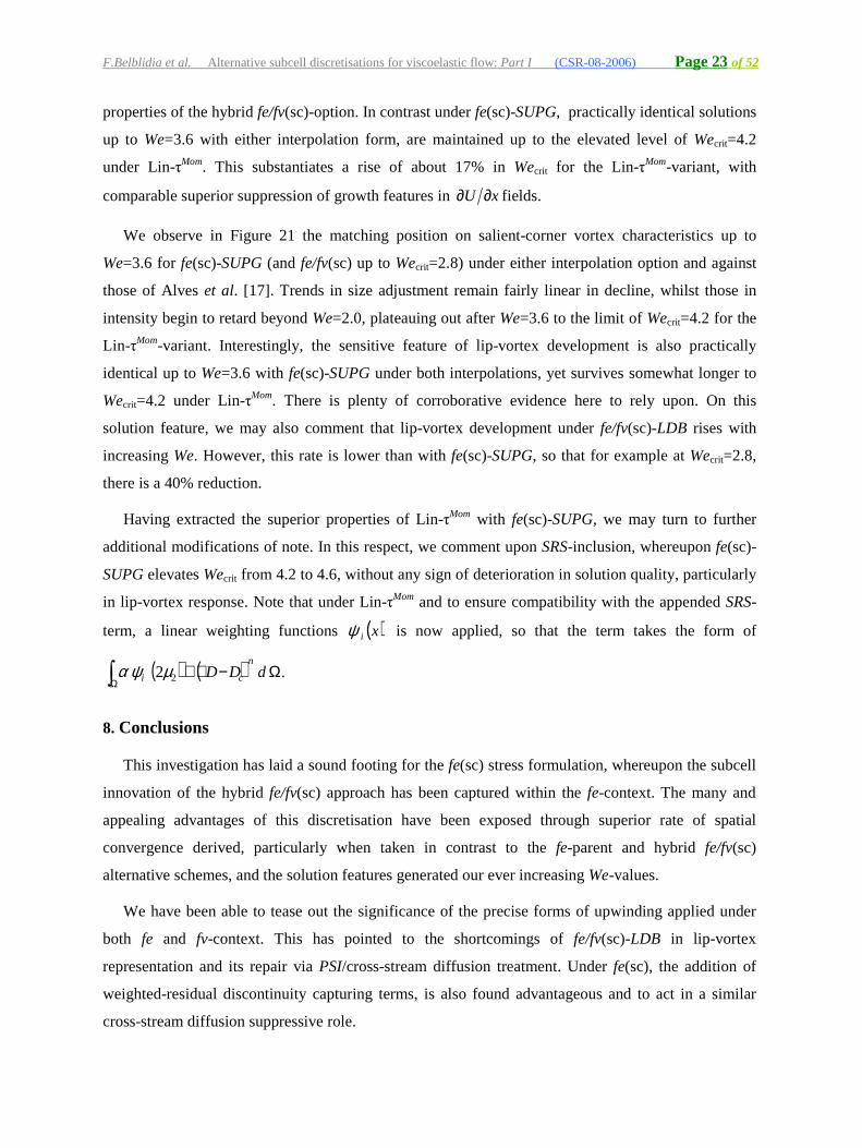
in lip-vortex response. Note that under Lin-τMom and to ensure compatibility with the appended SRS-

term, a linear weighting functions ( )xiψ is now applied, so that the term takes the form of

( ) ( ) Ω−⋅∇∫Ω dDDn

ci 22µψα .

8. Conclusions

This investigation has laid a sound footing for the fe(sc) stress formulation, whereupon the subcell

innovation of the hybrid fe/fv(sc) approach has been captured within the fe-context. The many and

appealing advantages of this discretisation have been exposed through superior rate of spatial

convergence derived, particularly when taken in contrast to the fe-parent and hybrid fe/fv(sc)

alternative schemes, and the solution features generated our ever increasing We-values.

We have been able to tease out the significance of the precise forms of upwinding applied under

both fe and fv-context. This has pointed to the shortcomings of fe/fv(sc)-LDB in lip-vortex

representation and its repair via PSI/cross-stream diffusion treatment. Under fe(sc), the addition of

weighted-residual discontinuity capturing terms, is also found advantageous and to act in a similar

cross-stream diffusion suppressive role.


The further considerations of strain-rate stabilisation and stress-momentum interpolation complete

the present study. Here, SRS is again found to enhance stability properties of all schemes considered,

with significant impact upon Wecrit elevation. The most impressive Wecrit achieved is under fe/fv(sc)-

LDB, where the level of 5.9 is attained, underlying the lip-vortex suppression. Under the fe(sc)-form,

both SUPG and SUPG-DC equate Wecrit at the level of 4.3.

Stress-momentum interpolation also proves optimal in the linear subcell form for these linear

stress approximations. This is felt principally through enhancement in stability properties, so for

example, raising fe(sc)-SUPG Wecrit from 4.3 to 4.6, upon switching between quadratic stress

interpolation on the parent element to linear on the subcell in the momentum equation (τMom(par) to

τMom(sc)). This is achieved without any sign of deterioration in solution quality. It is paramount to

report that all schemes investigated here, being under fe(sc) or fe/fv(sc), provide similar response with

regard to salient-corner characteristics. The enhanced stability observed under fe(sc) has not affected

lip-vortex intensity at sub-critical levels of We, through discontinuity capturing, or stain-rate

stabilisation, or switching to linear stress-momentum interpolation. In contrast under the fe/fv(sc)-

context, lip-vortex intensity has been found to be sensitive to the particular numerical treatment

applied.


References

[1] P. Wapperom and M.F. Webster, A second-order hybrid finite-element/volume method for viscoelastic flows, J. Non-Newtonian Fluid Mech. 79 (1998) 405-431.

[2] P. Wapperom and M.F. Webster, Simulation for viscoelastic flow by a finite volume/element method, Comp. Meth. Appl. Mech. Eng. 180 (1999) 281-304.

[3] M. Aboubacar and M.F. Webster, A cell-vertex finite volume/element method on triangles for abrupt contraction viscoelastic flows, J. Non-Newtonian Fluid Mech. 98 (2001) 83-106.

[4] M. Aboubacar, H. Matallah, H.R. Tamaddon-Jahromi and M.F. Webster, Numerical prediction of extensional flows in contraction geometries: hybrid finite volume/element method, J. Non-Newtonian Fluid Mech. 104 (2002) 125-164.

[5] M. Aboubacar, H. Matallah and M.F. Webster, Highly elastic solutions for Oldroyd-B and Phan-Thien/Tanner fluids with a finite volume/element method: planar contraction flows, J. Non-Newtonian Fluid Mech. 103 (2002) 65-103.

[6] I.J. Keshtiban, F. Belblidia and M.F. Webster, Numerical simulation of compressible viscoelastic liquids, J. Non-Newtonian Fluid Mech. 122 (2004) 131-146.

[7] I.J. Keshtiban, F. Belblidia and M.F. Webster, Computation of incompressible and weakly-compressible viscoelastic liquids flow: finite element/volume schemes, J. Non-Newtonian Fluid Mech. 126 (2005) 123-143.

[8] F. Belblidia, I.J. Keshtiban and M.F. Webster, Stabilised computations for viscoelastic flows under compressible implementations, J. Non-Newtonian Fluid Mech. 134 (2006) 56-76.

[9] J.M. Marchal and M.J. Crochet, A new mixed finite element for calculating viscoelastic flow, J. Non-Newtonian Fluid Mech. 26 (1987) 77-114.

[10] F.G. Basombrio, G.C. Buscaglia and E.A. Dari, Simulation of highly elastic fluid flows without additional numerical diffusivity, J. Non-Newtonian Fluid Mech. 39 (1991) 189-206.

[11] F.P.T. Baaijens, Numerical analysis of unsteady viscoelastic flow, Comp. Meth. Appl. Mech. Eng. 94 (1992) 285-299.

[12] E.O.A. Carew, P. Townsend and M.F. Webster, On a discontinuity capturing technique for Oldroyd-B fluids, J. Non-Newtonian Fluid Mech. 51 (1994) 231.

[13] F. Shakib, Finite Element Analysis of the Compressible Euler and Navier-Stokes Equations, Ph.D. Dissertation, Stanford University, Department of Mechanical Engineering (1988).

[14] H. Matallah, P. Nithiarasu and M.F. Webster, Stabilisation techniques for viscoelastic flows, ECCOMAS Conference, (2001).

[15] R. Guénette and M. Fortin, A new mixed finite element method for computing viscoelastic flows, J. Non-Newtonian Fluid Mech. 60 (1995) 27-52.

[16] J. Sun, N. Phan-Thien and R.I. Tanner, An adaptive viscoelastic stress splitting scheme and its applications: AVSS/SI and AVSS/SUPG, J. Non-Newtonian Fluid Mech. 65 (1996) 75-91.


[17] M.A. Alves, P.J. Oliveira and F.T. Pinho, Benchmark solutions for the flow of Oldroyd-B and PTT fluids in planar contractions, J. Non-Newtonian Fluid Mech. 110 (2003) 45-75.

[18] P.J. Oliveira and F.T. Pinho, Plane contraction flows of upper convected Maxwell and Phan-Thien-Tanner fluids as predicted by a finite-volume method, J. Non-Newtonian Fluid Mech. 88 (1999) 63-88.

[19] M. Renardy, Current issues in non-Newtonian flows: a mathematical perspective, J. Non-Newtonian Fluid Mech. 90 (2000) 243-259.

[20] H. Matallah, P. Townsend and M.F. Webster, Recovery and stress-splitting schemes for viscoelastic flows, J. Non-Newtonian Fluid Mech. 75 (1998) 139-166.

[21] M.F. Webster, H. Matallah and K.S. Sujatha, Sub-cell approximations for viscoelastic flows-filament stretching, J. Non-Newtonian Fluid Mech. 126 (2005) 187-205

[22] M.F. Webster, I.J. Keshtiban and F. Belblidia, Computation of weakly-compressible highly-viscous liquid flows, Eng. Comput. 21 (2004) 777-804.

[23] E.O.A. Carew, P. Townsend and M.F. Webster, A Taylor-Petrov-Galerkin algorithm for viscoelastic flow, J. Non-Newtonian Fluid Mech. 50 (1993) 253-287.

[24] M.F. Webster, H.R. Tamaddon-Jahromi and M. Aboubacar, Time-dependent algorithm for viscoelastic flow-finite element/volume schemes, Num. Meth. Partial Diff. Equ. 21 (2005) 272-296.

[25] M. Aboubacar and M.F. Webster, Development of an optimal hybrid finite volume/element method for viscoelastic flows, Int. J. Num. Meth. Fluids 41 (2003) 1147-1172.

[26] M.E. Hubbard and P.L. Roe, Multidimensional upwind fluctuation disctribution schemes for scalar dependent problems, Int. J. Num. Meth. Fluids 33 (2000) 711-736.

[27] H. Deconinck, P.L. Roe and R. Struijs, A multidimensional generalization of Roe's flux difference splitter for the Euler equations, Comput. & Fluids 22 (1993) 215-222.

[28] A. Jameson and D. Mavriplis, Finite volume solution of the two-dimensional Euler equations on a regular triangular mesh, AIAA 24 (1986) 611-618.

[29] K.W. Morton, P.I. Crumpton and J.A. Mackenzie, Cell vertex methods for inviscid and viscous flows, Comput. & Fluids 22 (1993) 91-102.

[30] M.S. Chandio, K.S. Sujatha and M.F. Webster, Consistent hybrid finite volume/element formulations: model and complex viscoelastic flows, Int. J. Num. Meth. Fluids 45 (2004) 495-471.

[31] U. Ghia, K.N. Ghia and C. Shin, High-Re solutions for incompressible flow using the Navier-Stokes equations and a multigrid method, J. Comp. Physics 48 (1982) 387-411.

[32] P.N. Shankar and M.D. Deshpande, Fluid mechanics in the driven cavity, Annu. Rev. Fluid Mech. 32 (2000) 93-136.


[33] R. Peyret and T.D. Taylor, Computational Methods for Fluid Flow, Springer-Verlag, New York, (1983).

[34] M. Renardy, Stress integration for the constitutive law of the upper convected Maxwell fluid near the corners in a driven cavity, J. Non-Newtonian Fluid Mech. 112 (2003) 77-84.

[35] R. Fattal and R. Kupferman, Constitutive laws for the matrix-logarithm of the conformation tensor, J. Non-Newtonian Fluid Mech. 123 (2004) 281.

[36] R. Fattal and R. Kupferman, Time-dependent simulation of viscoelastic flows at high Weissenberg number using the log-conformation representation, J. Non-Newtonian Fluid Mech. 126 (2005) 23-37.

[37] A. Afonso, M.A. Alves, F.T. Pinho and P.J. Oliveira, Benchmark calculations of viscoelastic flows with a finite-volume method using the log-conformation approach, 3rd Annual European Rheology Conference: AERC, (2006), 197.

[38] R.E. Evans and K. Walters, Flow characteristics associated with abrupt changes in geometry in the case of highly elastic liquids, J. Non-Newtonian Fluid Mech. 20 (1986) 11-29.

[39] R.E. Evans and K. Walters, Further remarks on the lip-vortex mechanism of vortex enhancement in planar-contraction flows, J. Non-Newtonian Fluid Mech. 32 (1989) 95-105.

[40] D.V. Boger, Viscoelastic flows through contractions, Annual Rev. Fluid Mech. 19 (1987) 157-182.

[41] J.P. Rothstein and G.H. McKinley, Extensional flow of a polystyrene Boger fluid through a 4:1:4 axisymmetric contraction/expansion, J. Non-Newtonian Fluid Mech. 86 (1999) 61-88.

[42] L.E. Rodd, T.P. Scott, D.V. Boger, J.J. Cooper-White and G.H. McKinley, The inertio-elastic planar entry flow of low-viscosity elastic fluids in micro-fabricated geometries, J. Non-Newtonian Fluid Mech. 129 (2005) 1-22.

[43] N.D. Waters and M.J. King, Unsteady flow of an elasto-viscous liquid, Rheol. Acta 9 (1970) 11-29.



F. Belblidia, H. Matallah, B. Puangkird and M. F. Webster

List of Tables:

Table I. Variables interpolations and definitions

Table II. Order of accuracy for velocity and stress, three scheme variants, cavity flow

Table III. Wecrit, ττττpeak and vortices characteristics, various schemes, contraction flow

Table IV. Wecrit, ττττpeak and vortices characteristics, various SRS-schemes, contraction flow

Table V. Wecrit, ττττpeak and vortices characteristics, various Lin-τMom-fe(sc)-schemes, with and

without SRS contraction flow

List of Figures:

Figure 1. a) Parent fe and fv-subcells, MDC area for node l, b) LDB-scheme representation

Figure 2. Lid-driven cavity mesh with boundary conditions

Figure 3. Contraction flows: a) schema, b) mesh refinement M1-M3 around contraction (elements, nodes, d.o.f., rmin)

Figure 4. Spatial error norm plots: three schemes, velocity and stress

Figure 5. Temporal convergence for Re = 0: a) mesh 80x80 and three schemes, (left) stress, (middle) velocity and (right) pressure; b) stress temporal convergence for different mesh-size

Figure 6. Streamlines, We=0.25: (left) three schemes, Re=0; (right) fe/fv(sc), Re=0, Re=100

Figure 7. Symmetry-line velocity profiles across cavity, fe/fv-scheme: a) We=0, Re=100; b) We=0.25, Re=0 and Re=100

Figure 8. Solution fields, fe/fv(sc) scheme, Re=0 and Re=100; ux, vy, τxx, τxy, τyy and p variables

Figure 9. Mesh refinement: τxx-contour fields, We=1.5, a) mesh M1, b) M2 and c) M3

Figure 10. Stress at We=2.5; a) (τxx, τxy)-profiles, downstream-wall, (left) τxx, (right) τxy; b) (τxx, τxy)-fields, (top) τxx, (bottom) τxy; under (left) fe/fv(sc): LDB, PSI, and (right) fe(sc): SUPG, SUPG-DC


Figure 11. Velocity-gradients at We=2.5; (top) ∂u/∂x-fields, (bottom) ∂u/∂y-fields; under (left) fe/fv(sc): LDB, PSI, and (right) fe(sc): SUPG, SUPG-DC

Figure 12. Stress profiles, increasing We; τxx-profiles, downstream-wall with zoom around corner; under (left) fe/fv(sc): a) LDB, b) PSI, and (right) fe(sc): c) SUPG, d) SUPG-DC

Figure 13. Stress fields, Wecrit; (top) τxx, (bottom) τxy; under (left) fe/fv(sc): LDB, PSI, and (right) fe(sc): SUPG, SUPG-DC

Figure 14. Vortex behaviour, increasing We; (top) vortex trends; (bottom) streamlines, We=2.0 and Wecrit, with zoom around corner; under (left) fe/fv(sc): a) LDB, b) PSI, and (right) fe(sc): c) SUPG, d) SUPG-DC

Figure 15. SRS-Stress profiles, increasing We; τxx-profiles, (i) window without SRS-effect, (ii) zoom around corner; under (left) fe/fv(sc): a) LDB-SRS, b) PSI-SRS, and (right) fe(sc): c) SUPG-SRS, d) SUPG-DC-SRS

Figure 16. Evolution-factor fields; no-SRS, We=2.5; SRS, We=2.5, We=4.0, Wecrit; under (left) fe/fv(sc): a) LDB, b) PSI, and (right) fe(sc): c) SUPG, d) SUPG-DC

Figure 17. SRS-Stress fields, Wecrit; (top) τxx, (bottom) τxy; under (left) fe/fv(sc): a) LDB-SRS, b) PSI-SRS, and (right) fe(sc): c) SUPG-SRS, d) SUPG-DC-SRS

Figure 18. SRS-vortex behaviour, increasing We; (top) vortex trends; (bottom) streamlines, We=2.0 and Wecrit, with zoom around corner; under (left) fe/fv(sc): a) LDB-SRS, b) PSI-SRS, and (right) fe(sc): c) SUPG-SRS, d) SUPG-DC-SRS

Figure 19. fe/fv(sc)-lip-vortex behaviour, Wecrit; (i) under mesh type 1, a) LDB, b) LDB-SRS, c) PSI, d) PSI-SRS; (ii) under mesh type 2, e) LDB, f) LDB-SRS; (top) velocity-vectors, (bottom) lip-vortex

Figure 20. Stress profiles, increasing We; τxx-profiles, downstream-wall with zoom around corner; under (left) Quad-τMom, (right) Lin-τMom; a) fe/fv(sc)-LDB, b) fe(sc)-SUPG

Figure 21. Vortex behaviour, increasing We; (top) vortex trends; (bottom) fe(sc)-streamlines, We=2.0 and Wecrit, with zoom around corner; under (left) Quad-τMom, (right) Lin-τMom


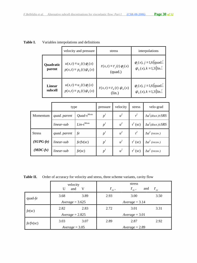
Table I. Variables interpolations and definitions

velocity and pressure stress interpolations

Quadratic

parent

)()(),( xtutxu jj φ=

)()(),( xtptxp kk ψ=

)()(),( xttx jj φττ =

(quad.)

( )quad.6,1),( =jxjφ

( )lin.3,1),( =kxkψ

Linear subcell

)()(),( xtutxu jj φ=

)()(),( xtptxp kk ψ=

)()(),( xttx kk ψττ =

(lin.)

( )quad.6,1),( =jxjφ

( )lin.3,1),( =kxkψ

type pressure velocity stress velo-grad

quad. parent Quad-τMom p1 u2 τ2 ∆u1

(disct.)±SRS Momentum

linear-sub Lin-τMom p1 u2 τ1 (sc) ∆u1

(disct.)±SRS

quad. parent fe p1 u2 τ2 ∆u2 (recov.)

linear-sub fe/fv(sc) p1 u2 τ1 (sc) ∆u2 (recov.)

Stress

(SUPG-fe)

(MDC-fv) linear-sub fe(sc) p1 u2 τ1 (sc) ∆u2 (recov.)

Table II. Order of accuracy for velocity and stress, three scheme variants, cavity flow

velocity

U and V

stress

xxτ , xyτ , and yyτ

3.68 3.89 2.93 3.00 3.50 quad-fe

Average = 3.625 Average = 3.14

2.82 2.83 2.72 3.01 3.31 fe(sc)


3.03 3.07 2.89 2.87 2.92 fe/fv(sc)



Table III. Wecrit, τpeak and vortices characteristics, various schemes, contraction flow

fe/fv(sc) fe(sc)

quad-fe [7] LDB PSI SUPG SUPG-DC

Critical We 2.2 2.8 2.5 3.6 2.8

Peak τxx at Wecrit 76.3 103.8 89.7 119.9 105.3

τxx at We=2.5 - 101.7 89.7 100.5 91.2

Table IV. Wecrit, τpeak and vortices characteristics, various SRS-schemes, contraction flow

SRS

fe/fv(sc) fe(sc)

LDB PSI SUPG SUPG-DC

Critical We 5.9 4.0 4.3 4.3

Peak τxx at Wecrit 157.3 116.4 122.2 121.7

τxx at We=2.5 91.9 99.6 95.2 87.7

Table V. Wecrit, τpeak and vortices characteristics, various Lin-τMom-fe(sc)-schemes, with and without SRS contraction flow

no-SRS (SUPG) SRS (SUPG)

Quad-τMom Lin-τMom Quad-τMom Lin-τMom

Critical We 3.6 4.2 4.3 4.6

Peak τxx at Wecrit 119.9 124.6 122.2 118.9

τxx at We=2.5 100.5 98.2 95.2 93.6

τxx at We=3.5 116.2 113.6 114.2 111.6


Figure 1. a) Parent fe and fv-subcells, MDC area for node l, b) LDB-scheme representation

fe-cell

l(MDC)

T1

T2

T3

T4T5

T6

αiT

j

lk

j

k

i k

j

γ1

γ2

a)

b)


Figure 2. Lid-driven cavity mesh with boundary conditions

x

y

0 0.2 0.4 0.6 0.8 10

0.2

0.4

0.6

0.8

1moving lid U = x2 (1-x)2 →

nosl

ipw

allU

=V

=0

no slip wallU=V=0

noslip

wallU

=V

=0

fixedτ=0, p=0


Figure 3. Contraction flows: a) schema, b) mesh refinement M1-M3 around contraction (elements,

nodes, d.o.f., rmin)

7.

27.5

76.5

1

U =V =0

U=0, τ =0

P=0, U (by B.I.), V=0

U =V =0

4

y x

U , τxx, τxy Waters & King V =0 =τ yy

XS

a)

b)

M1: (980,2105,8983,0.025) M2: (1140,2427,9708,0.023) M3: (2987,6220,14057,0.006)


Figure 4. Spatial error norm plots: three schemes, velocity and stress

∆hE

rror

norm

(Vy)

0.01 0.015 0.02 0.02510-7

10-6

10-5

10-4

∆h

Err

orno

rm(U

x)

0.01 0.015 0.02 0.02510-7

10-6

10-5

10-4 fefe(sc)fe/fv(sc)

∆h

Err

orno

rm(τ

xy)

0.01 0.015 0.02 0.02510-4

10-3

10-2

10-1

∆h

Err

orno

rm(τ

xx)

0.01 0.015 0.02 0.02510-4

10-3

10-2

10-1

∆h

Err

orno

rm(τ

yy)

0.01 0.015 0.02 0.02510-4

10-3

10-2

10-1

fefe(sc)fe/fv(sc)

Ux Vy

τxx τyy τxy


Figure 5. Temporal convergence for Re = 0: a) mesh 80x80 and three schemes, (left) stress, (middle) velocity and (right) pressure; b) stress temporal convergence for different mesh-size

τ U P

fe(sc) fe fe/fv(sc)

a)

b) τ


Figure 6. Streamlines, We=0.25: (left) three schemes, Re=0; (right) fe/fv(sc), Re=0, Re=100

1 2 3 4

1

2

3

4

567

8

Level S

8 5.0E-077 0.0E+006 -5.0E-065 -5.0E-044 -1.0E-023 -3.0E-022 -5.0E-021 -7.0E-02

Re=0- - - - Re=100

fe/fv(sc)

1

2

3

4

56 87

Level S

8 5.0E-077 0.0E+006 -5.0E-065 -5.0E-044 -1.0E-023 -3.0E-022 -5.0E-021 -7.0E-02

fefe(sc)

fe/fv(sc)

a) three schemes, Re=0 b) fe/fv(sc), Re=0, 100


Figure 7. Symmetry-line velocity profiles across cavity, fe/fv-scheme: a) We=0, Re=100; b) We=0.25, Re=0 and Re=100

a) We=0, Re=100 b) We=0.25, Re=0 and 100

Velocity

Ver

tical

/Hor

izon

talD

ista

nce

-0.25 0 0.25 0.5 0.75 10

0.25

0.5

0.75

1

Ghiaux ⊗ y, Re = 100Ghiauy ⊗ x, Re = 100Newtonianux ⊗ y, Re = 100Newtonianuy ⊗ x, Re = 100

Velocity

Ver

tical

/Hor

izon

talD

ista

nce

-0.25 0 0.25 0.5 0.75 10

0.25

0.5

0.75

1

ux ⊗ y, Re = 0uy ⊗ x, Re = 0ux ⊗ y, Re = 100uy ⊗ x, Re = 100

uy, y=1/2 ux, x=1/2


Figure 8. Solution fields, fe/fv(sc) scheme, Re=0 and Re=100; ux, vy, τxx, τxy, τyy and p variables

6

78

54

3

21

Level Vy

9 0.208 0.157 0.106 0.055 0.004 -0.053 -0.102 -0.151 -0.20

Re = 0Re = 100

1

2

3

46

7

8

9

5 5

5

5

Level Ux

7 0.96 0.75 0.54 0.33 0.12 0.01 -0.1

Re = 0Re = 100

1

2 2

23

4576

1

2 34

56

3

1

123

1

Level Txx

6 30.005 20.004 10.003 5.002 1.001 0.00

Re = 0Re = 100

1

1

1

1

2

3 4 5 6

3

42

15

6

8

101

Level p

12 24.0011 22.0010 20.009 18.008 16.007 14.006 12.005 10.004 8.003 6.002 4.001 2.00

Re = 0Re = 1005

12

3

4

5

6

7

89

1011122

1

12

3 3

41

Level Tyy

8 14.007 12.006 10.005 8.004 6.003 4.002 2.001 0.00

Re = 0Re = 100

8

1

2

1

2

1 1

3 45 6

11

2

2

3

2

3

3

Level Txy

6 5.005 4.004 3.003 2.002 1.001 0.00

Re = 0Re = 100

1

1

1

1

2

34

5 6

1

1

1

1


Figure 9. Mesh refinement: τxx-contour fields, We=1.5, a) mesh M1, b) M2 and c) M3

a) M1 b) M2 c) M3

fe(sc)

12

3 56

4 5

7 8 9

τxxmax= 39.5

5 4

7

21

3 46

98

5

τxxmax= 72.2

12

34

56

4

7 8 9

Level Txx9 15.008 5.007 3.006 2.505 2.004 1.503 1.002 -0.101 -0.20

τxxmax= 35.6


Figure 10. Stress at We=2.5; a) (τxx, τxy)-profiles, downstream-wall, (left) τxx, (right) τxy; b) (τxx, τxy)-fields, (top) τxx, (bottom) τxy; under (left) fe/fv(sc): LDB, PSI, and (right) fe(sc): SUPG, SUPG-DC

LDB PSI SUPG SUPG-DC

fe/fv(sc) fe(sc)

2

3

7

6

8

1

3 4

9

2

5

23

55

1

6

4

46 7

23

55

1

6

4

367

23

55

1

6

4

467

23

55

1

6

4

467

Level Txy

7 3.06 2.05 1.04 0.53 0.22 0.11 0.0

2

35

7

1

4

6

9

2

8

3

Level Txx

9 30.08 15.07 5.06 3.05 2.54 2.03 1.82 -0.11 -0.2

2

35

8

1

4

7

6

2

3

92

3

7

5

8

1

3 4

6

9

2

XT

xy22 24 26 28

0

20

40

fe/fv(sc) LDBfe(sc) SUPGfe/fv(sc) PSIfe(sc) SUPG-DC

X

Txx

22 24 26 28

0

40

80

120

a) (τxx, τxy)-profiles

b) (τxx, τxy)-fields


Figure 11. Velocity-gradients at We=2.5; (top) ∂u/∂x-fields, (bottom) ∂u/∂y-fields; under (left) fe/fv(sc): LDB, PSI, and (right) fe(sc): SUPG, SUPG-DC

∂u/∂x

∂u/∂y

LDB PSI SUPG SUPG-DC fe/fv(sc) fe(sc)

2

1

4

23

3

5

57

2

1

4

23

3

576

Level ∂U/∂y

7 3.006 2.505 2.004 1.003 0.502 0.201 0.00

2

1

4

23

3

5

76

2

1

4

23

3

5

76

1

5

2

4 6

6

3

3

7

1

5

2

4

6 5

3

3

76

1

5

2

4 6

6

3

3

7

Level ∂U/∂x

7 0.506 0.005 -0.024 -0.073 -0.252 -0.501 -1.00 1

5

2

4 6

6

3

3

75


Figure 12. Stress profiles, increasing We; τxx-profiles, downstream-wall with zoom around corner; under (left) fe/fv(sc): a) LDB, b) PSI, and (right) fe(sc): c) SUPG, d) SUPG-DC

X

Txx

20 25 30 35

0

40

80

120 We=1.0We=2.0We=2.5We=2.8

X

Txx

20 25 30 35

0

40

80

120 We=1.0We=2.0We=2.5

X

Txx

20 25 30 35

0

40

80

120 We=1.0We=2.0We=2.5We=2.8

X

Txx

20 25 30 35

0

40

80

120 We=1.0We=2.0We=2.5We=3.0We=3.6

a) LDB

b) PSI

c) SUPG

d) SUPG-DC

fe/fv(sc) fe(sc)


Figure 13. Stress fields, Wecrit; (top) τxx, (bottom) τxy; under (left) fe/fv(sc): LDB, PSI, and (right) fe(sc): SUPG, SUPG-DC

LDB PSI SUPG SUPG-DC fe/fv(sc) fe(sc)

2

35

7

1

4

6

9

2

8

3Level Txx

9 30.08 15.07 5.06 3.05 2.54 2.03 1.82 -0.11 -0.2

2

35

8

1

4

7

6

2

3

9

2

3

7

5

8

3 4

6

9

22

3

7

6

8

1

3 4

9

2

5

23

55

1

6

5

46 7

23

5

5

1

6

5

467

23

55

1

6

4

467

23

45

1

6

4

467

Level Txy

7 3.06 2.05 1.04 0.53 0.22 0.11 0.0

Wecrit=2.8 Wecrit=2.5 Wecrit=3.6 Wecrit=2.8

τxx

τ

xy


Figure 14. Vortex behaviour, increasing We; (top) vortex trends; (bottom) streamlines, We=2.0 and Wecrit, with zoom around corner; under (left) fe/fv(sc): a) LDB, b) PSI, and (right) fe(sc): c) SUPG, d) SUPG-DC

We

Siz

e

0 1 2 3 40.8

1

1.2

1.4

1.6

We

Inte

nsity

103

0 1 2 3 40

0.4

0.8

1.2

Alves et al. (2003)fe/fv(sc) LDBfe/fv(sc) PSIfe(sc) SUPGfe(sc) DC+SUPG

We

Lip

-int

ensi

ty1

03

0 1 2 3 4

0

0.2

0.4

0.6

fe/fv(sc)

We=

2.0

ψsal= 0.491e-3

X=1.22

ψlip= 0.085e-3

X=0.95

ψsal= 0.233e-3

ψlip= 0.546e-3

We=

3.6

We=

2.0

ψsal= 0.511e-3

X=1.22

ψlip= 0.036e-3

X=1.12

ψsal= 0.398e-3

ψlip= 0.155e-3

We=

2.5

We=

2.0

ψsal= 0.478e-3

X=1.22

ψlip= 0.073e-3

X=1.12

ψsal= 0.277e-3

ψlip= 0.263e-3

We=

2.8

X=1.05ψsal= 0.325e-3

ψlip= 0.107e-3

We=

2.8

We=

2.0

ψsal= 0.510e-3

X=1.23

ψlip= 0.015e-3

a) LDB

d) SUPG-DC b) PSI

c) SUPG

fe(sc)


Figure 15. SRS-Stress profiles, increasing We; τxx-profiles, (i) window without SRS-effect, (ii) zoom around corner; under (left) fe/fv(sc): a) LDB-SRS, b) PSI-SRS, and (right) fe(sc): c) SUPG-SRS, d) SUPG-DC-SRS

fe/fv(sc)

ii) zoom

i) no-SRS

a) LDB-SRS

i) no-SRS

fe(sc)

c) SUPG-SRS ii) zoom X

Txx

20 25 30 35 40

0

40

80

120

160We=1.0We=2.0We=2.5We=3.0We=4.0We=5.0We=5.9

X

Txx

20 25 30 35 40

0

40

80

120

160We=1.0We=2.0We=2.5We=3.0We=4.0We=4.3

22 24 26

0

40

80

120

160 We=2.5We=2.8

22 24 26

0

40

80

120

160 We=2.5We=3.6

ii) zoom ii) zoom

i) no-SRS i) no-SRS

X

Txx

20 25 30 35 40

0

40

80

120

160We=1.0We=2.0We=2.5We=3.0We=4.0We=4.3

X

Txx

20 25 30 35 40

0

40

80

120

160We=1.0We=2.0We=2.5We=3.0We=4.0

22 24 26

0

40

80

120

160 We=2.5

22 24 26

0

40

80

120

160 We=2.5We=2.8

d) SUPG-DC-SRS b) PSI-SRS


Figure 16. Evolution-factor fields; no-SRS, We=2.5; SRS, We=2.5, We=4.0, Wecrit; under (left) fe/fv(sc): a) LDB, b) PSI, and (right) fe(sc): c) SUPG, d) SUPG-DC

a) LDB b) PSI c) SUPG d) SUPG-DC

fe/fv(sc) fe(sc)

no-S

RS

SRS

SRS

SRS

SUPG-DC

Smin=-110.7Smax= 106.3

Smin=-76.3Smax= 84.9

Smin=-62.9Smax= 103.8

Smin=-65.1Smax=108.0

Smin=-74.5Smax= 93.2

We=

4.0

Smin=-1196.0Smax= 1322.5

Smin=-281.8Smax= 161.2

Smin=-475.4Smax= 197.4

SUPG

Smin=-103.7Smax= 104.2

Smin=-69.6Smax= 106.8

Smin=-55.4Smax= 109.1

We=

2.5

Smin=-148.7Smax= 356.8

We cr

it

Smin=-5340.7Smax= 3206.7

S6040200

-20-40-60W

e=2.

5

Smin=-27.2Smax= 484.6

Smin=-23.8Smax= 311.5


Figure 17. SRS-Stress fields, Wecrit; (top) τxx, (bottom) τxy; under (left) fe/fv(sc): a) LDB-SRS, b) PSI-SRS, and (right) fe(sc): c) SUPG-SRS, d) SUPG-DC-SRS

a) LDB-SRS b) PSI-SRS c) SUPG-SRS d) SUPG-DC-SRS

fe/fv(sc) fe(sc)

Txy

T

xx

23

6

5

1

5

5

4

67 4

23

6

5

1

5

5

4

67

4

23

6

5

1

5

5

4

67

4

45

8

4 3

76

2

3

9

Wecrit=4.02

3

7

5

8

3 4

6

9

Wecrit=4.3

3

7

6

8

3 4

9

2

5

Wecrit=4.32

46

8

5

7

9 8

43

Level Txx9 30.08 15.07 5.06 3.05 2.54 2.03 1.82 -0.11 -0.2

Wecrit=5.9

43

45

1

5

5

2

67

3

Level Txy7 3.06 2.05 1.04 0.53 0.22 0.11 0.0


Figure 18. SRS-vortex behaviour, increasing We; (top) vortex trends; (bottom) streamlines, We=2.0 and Wecrit, with zoom around corner; under (left) fe/fv(sc): a) LDB-SRS, b) PSI-SRS, and (right) fe(sc): c) SUPG-SRS, d) SUPG-DC-SRS

We

Siz

e

0 1 2 3 4 5 60.6

0.8

1

1.2

1.4

1.6

We

Lip

-inte

nsity

103

0 1 2 3 4 5 60

0.4

0.8

1.2

1.6

We

Inte

nsi

ty10

3

1 2 3 4 5 60

0.4

0.8

1.2

Alves et al. (2003)fe/fv(sc) LDB SRSfe/fv(sc) PSI SRSfe(sc) SUPG SRSfe(sc) DC+SUPG SRS

We=

2.0

ψlip= 0.118e-3

X=1.25

ψsal= 0.497e-3

X=0.69

ψsal= 0.009e-3

We=

5.9

ψsal= 0.114e-3

We=

2.0

ψsal= 0.508e-3

X=1.21

ψlip= 0.188e-3

X=0.88

ψsal= 0.201e-3

ψlip= 0.615e-3

We=

4.0

We=

2.0

ψsal= 0.487e-3

X=1.21

ψlip= 0.225e-3

X=0.87

ψsal= 0.197e-3

ψlip= 1.326e-3

We=

4.3

X=0.87

ψsal= 0.220e-3

ψlip= 1.398e-3W

e=4.

3W

e=2.

0

ψsal= 0.497e-3

X=1.23

ψlip= 0.209e-3

a) LDB-SRS

b) PSI-SRS

c) SUPG-SRS

d) SUPG-DC-SRS

fe/fv(sc) fe(sc)


Figure 19. fe/fv(sc)-lip-vortex behaviour, Wecrit; (i) under mesh type 1, a) LDB, b) LDB-SRS, c) PSI, d) PSI-SRS; (ii) under mesh type 2, e) LDB, f) LDB-SRS; (top) velocity-vectors, (bottom) lip-vortex

Mesh Type 1 Mesh Type 2

ψψlip=-0.752 e-3 ψlip=-0.859 e-3ψlip=-0.107 e-3 ψlip=-0.009 e-3 ψlip=-0.155 e-3

ψψlip=-0.615 e-3

a) LDB Wecrit =2.8

i) Mesh 1

b) LDB-SRS Wecrit =5.9

c) PSI Wecrit =2.5

d) PSI-SRS Wecrit =4.0

e) LDB Wecrit =2.8

f) LDB-SRS Wecrit =5.0

ii) Mesh 2


Figure 20. Stress profiles, increasing We; τxx-profiles, downstream-wall with zoom around corner; under (left) Quad-τMom, (right) Lin-τMom; a) fe/fv(sc)-LDB, b) fe(sc)-SUPG

X

Txx

25 30 35

0

40

80

120We=1.0We=2.0We=2.5We=3.0We=3.6We=4.2

X

Txx

25 30 35

0

40

80

120We=1.0We=2.0We=2.5We=3.0We=3.6

X

Txx

25 30 35

0

40

80

120We=1.0We=2.0We=2.5We=2.8

XT

xx25 30 35

0

40

80

120We=1.0We=2.0We=2.5We=2.8

Lin-τMom Quad-τMom

a) L

DB

b)

SU

PG


Figure 21. Vortex behaviour, increasing We; (top) vortex trends; (bottom) fe(sc)-streamlines,

We=2.0 and Wecrit, with zoom around corner; under (left) Quad-τMom, (right) Lin-τMom

We=

2.0

ψsal= 0.515e-3

X=1.22

ψlip= 0.082e-3

X=0.88

ψsal= 0.235e-3

ψlip= 0.703e-3

We=

4.2

We=

3.6

ψsal= 0.245e-3

X=0.98

ψlip= 0.525e-3

We=

2.0

ψsal= 0.491e-3

X=1.22

ψlip= 0.085e-3

X=0.95

ψsal= 0.233e-3

ψlip= 0.546e-3

We=

3.6

Lin-τMom Quad-τMom fe(sc)

We

Lip

-in

tens

ity10

3

0 1 2 3 4

0

0.2

0.4

0.6

0.8

We

Inte

nsi

ty1

03

0 1 2 3 40

0.2

0.4

0.6

0.8

1

1.2

We

Siz

e

0 1 2 3 40.8

1

1.2

1.4

1.6

Alves et al. (2003)fe/fv(sc), Quad/LinτMom

fe(sc), QuadτMom

fe(sc), LinτMom

Date post:	28-Feb-2022
Category:	Documents
Upload:	others
View:	1 times
Download:	0 times

FB SubmitCSR08-06 Part1 - Swansea University

Documents