Methods for Multivariate Analyses in Neuroimaging Fábio Daniel Santos Ferreira MASTER’S DEGREE IN BIOMEDICAL ENGINEERING Physics Department Faculty of Sciences and Technology of University of Coimbra July 2014
Transcript
Methods for Multivariate Analyses in Neuroimaging
Fábio Daniel Santos Ferreira
MASTER’S DEGREE IN BIOMEDICAL ENGINEERING
Physics Department
Faculty of Sciences and Technology of University of Coimbra
July 2014
Methods for Multivariate Analyses in Neuroimaging
Author Supervisor
Fábio D. S. Ferreira Dr. João M. Pereira
Dissertation presented to the Faculty of Sciences and Technology of the
University of Coimbra to obtain a Master’s degree in Biomedical Engineering
Coimbra, 2014
v
This thesis was developed in collaboration with:
Faculty of Medicine of the University of Coimbra
Institute for Biomedical Imaging and Life Sciences
vi
vii
Esta cópia da tese é fornecida na condição de que quem a consulta reconhece que os
direitos de autor são pertença do autor da tese e que nenhuma citação ou informação
obtida a partir dela pode ser publicada sem a referência apropriada.
This copy of the thesis has been supplied on condition that anyone who consults it is
understood to recognize that its copyright rests with its author and that no quotation
from the thesis and no information derived from it may be published without proper
acknowledgement.
viii
ix
Esta tese é dedicada aos meus pais e à minha irmã,
x
xi
Acknowledgments
Várias são as pessoas responsáveis pela conclusão deste projeto e
consequentemente pela finalização do meu Mestrado Integrado em Engenharia
Biomédica. Em primeiro lugar, e como não poderia deixar de ser, quero agradecer ao
meu orientador Dr. João Pereira por toda ajuda prestada, por todo conhecimento
transmitido, por todo o seu empenho e dedicação neste projeto e por todo o seu
profissionalismo demonstrado como orientador de uma Tese de Mestrado. Um
obrigado por tudo!
Em seguida gostaria de agradecer a mais duas pessoas que ajudaram no
aperfeiçoamento do projeto. Em primeiro lugar, ao Dr. Miguel Patrício por seguir
sempre de perto o desenvolvimento do projeto e por disponibilizar a sua ajuda sempre
que necessário. A segunda pessoa é o Investigador João Duarte por estar sempre
disponível quando era necessário e por me transmitir o seu conhecimento em Machine
Learning, nomeadamente sobre Support Vector Machines.
Quero ainda agradecer à instituição acolhedora do meu projeto, o Instituto
Biomédico de Investigação de Luz e Imagem (IBILI) da Faculdade de Medicina da
Universidade de Coimbra, por me oferecer as condições de trabalho necessárias à
realização desta dissertação. Como não poderia deixar de ser, quero também
agradecer ao Prof. Doutor Miguel Castelo-Branco, coordenador científico do IBILI, por
criar diversas possibilidades para os alunos de Engenharia Biomédica contactarem com
o mundo da investigação biomédica. Quero ainda agradecer ao Prof. Doutor Miguel
Morgado, coordenador do curso de Mestrado Integrado em Engenharia Biomédica,
por toda a dedicação que tem oferecido na organização do curso e por estar sempre
disponível para ajudar.
Por fim, os mais importantes e sempre presentes nesta minha caminhada
académica pela cidade dos amores: a família e os amigos. Em relação à família, quero
destacar os meus pais e a minha irmã por estarem sempre presentes em todos os
momentos e pelo apoio incondicional. Quanto aos amigos, quero agradecer
especialmente: à Mafalda pela sua compreensão e cumplicidade, ao Gonçalo, ao
xii
Ricardo, ao Rocha, à Adriana, ao Levita, ao Miguel, ao Diogo, ao Gil, ao Fernando e ao
Filipe por partilharem Coimbra comigo. Um obrigado a todos por tudo!
xiii
Abstract
Neuroimaging is a vast area that includes a wide range of brain-mapping
techniques, each with specific information about the brain. As each technique has its
strengths and weaknesses, it is desirable to aim for multimodal studies to possibly
obtain more relevant information. Currently, the typical strategy in neuroimaging data
analysis consists of a massive univariate approach, using the General Linear Model
(GLM) in voxel based morphometry (VBM). However, this may be insufficient to
obtain a realistic analysis due to the complexity of the structure of the brain. This leads
to the application of multivariate methods, whereby information from different
modalities can be integrated. Support Vector Machines (SVMs) and related tools are
widely used, but these do not use statistical inference tests or provide p-values for
every voxel of an image, leading to difficulties in interpretation and generalization. As
such, this thesis focuses on implementation of inferential multivariate methods that are
both a natural extension of the univariate methods commonly used and allow for the
integration of the information from different imaging modalities. Given time and data
constraints, the focus of this thesis rested on two MRI contrasts: volumetric T1
(‘Anatomy’ scans) and T2 (‘Pathology’ scans) scans obtained from 42 control and 34
type II diabetes mellitus (T2DM) subjects. This simultaneous analysis is pertinent
because it is known that T2DM leads to gray matter atrophy and vasopathies that
predispose the brain to ischemia and subcortical lacunar infarcts. All inferential
methods were implemented in Matlab and were compared with those conducted with
SPM8 software. The classification method (SVM) was performed in the PRoNTo
toolbox. Results in both univariate and multivariate analyses showed gray matter
atrophy and possible vascular changes in the limbic lobe, sub-lobar, insular and
temporal areas of the T2DM brains. Furthermore, results indicate that the multivariate
methods may lead to more specific results than the univariate ones. A toolbox was
developed to be used in the software package SPM8, where the featured methods may
be made publicly available. Despite the limitations, notably that some of the pre-
requisites to perform multivariate statistical tests were not tested, this proof of
concept shows great promise. Future work will focus on surpassing these limitations
and on preparing the methods to be applied in other multimodal (PET, fMRI) studies.
xiv
Keywords: MRI, VBM, Type II Diabetes Mellitus, Multivariate GLM
xv
Resumo
A neuroimagem é uma vasta área que inclui uma ampla gama de técnicas de
mapeamento cerebral, cada uma com informações específicas sobre o cérebro. Como
cada técnica tem os seus pontos fortes e fracos, é desejável o uso de estudos
multimodais para possivelmente obter informação mais relevante. Atualmente, a
estratégia típica na análise de dados de neuroimagem consiste numa abordagem
univariada em massa, utilizando o Modelo Linear Geral (GLM, em inglês) no VBM
(Voxel Based Morphometry). Contudo, esta abordagem pode não ser suficiente para se
obter uma análise realista devido à complexidade da estrutura cerebral. Por isto surge
a necessidade do uso de métodos multivariados, através dos quais é possível integrar
informação de diferentes modalidades. As máquinas de vetores de suporte (SVMs, em
inglês) e outras ferramentas relacionadas são amplamente usadas, no entanto estas não
usam testes de inferência estatística ou fornecem valores p para cada voxel de uma
imagem, o que leva a dificuldades de interpretação e generalização. Portanto, esta tese
foca-se na implementação de métodos multivariados inferenciais que são uma extensão
natural dos métodos univariados já usados e, para além disto, permitem a integração
de diferentes modalidades de imagem. Com as limitações de tempo e de dados, o foco
desta tese recaiu sobre dois contrastes de Imagem por Ressonância Magnética (MRI,
em inglês): T1 (scans de 'Anatomia') e T2 (scans de ‘patologia’), obtidos de 42
controlos e de 34 pacientes com diabetes tipo 2. A análise simultânea destes dois
contrastes poderá possibilitar uma melhor compreensão desta patologia, uma vez que
se sabe que a diabetes tipo 2 contribui para a atrofia da massa cinzenta e vasopatias
que predispõem o cérebro a isquemia e enfartes lacunares subcorticais. Todos os
métodos inferenciais foram implementados em Matlab e comparados com os
realizados no software SPM8. O método de classificação (SVM) foi realizado na toolbox
PRoNTo. Os resultados, tanto das análises univariadas como das multivariadas,
revelaram atrofia da massa cinzenta e possíveis alterações vasculares no lobo límbico,
sub-lobar, áreas insulares e temporais do cérebro de doentes com diabetes tipo 2.
Para além disto, os resultados indicam que os métodos multivariados podem levar a
resultados mais específicos do que os univariados. Foi ainda preparada uma toolbox
para ser usada no pacote de software SPM8, onde os métodos desenvolvidos podem
ser disponibilizados publicamente. Apesar de algumas limitações, nomeadamente que
xvi
alguns dos pré-requisitos para a realização de testes estatísticos multivariados não
foram testados, esta prova de conceito apresenta-se promissora. O trabalho futuro
focar-se-á em superar estas limitações e preparar estes métodos para outros estudos
multimodais (PET, fMRI).
Palavras-chave: MRI, VBM, Diabetes tipo 2, GLM multivariado
xvii
Symbols & Abbreviations
Symbols
Residual variance estimates
, Sample mean vectors
Variance-covariance matrix
Fitted values matrix/vector
Weight vector
Degrees of freedom
Parameters estimates matrix/vector
Chi-square
A, M A and M matrices of multivariate contrast matrix
B0 Magnetic field
C, c Contrast matrix and contrast vector
f Larmor frequency
Mg Net magnetization vector
Mgxy Transversal net magnetization vector
Mgz Longitudinal net magnetization vector
R Multiple correlation coefficient
t, F t and F statistics
T2 Hotelling’s T2
Var Variance
X Design matrix
Y Observation vector/matrix
Gyromagnetic ratio
Residual errors matrix/vector
Wilk’s lambda
B, W Sum of squares and cross products matrices between and within
λ Eigenvalues
xviii
Abbreviations
ANCOVA Analysis of Covariance
ANOVA Analysis of Variance
CSF Cerebrospinal Fluid
DV Dependent Variable
fMRI functional Magnetic Resonance Imaging
FOV Field Of View
FT Fourier Transform
FWHM Full Width at Half Maximum
GLM General Linear Model
GM Gray Matter
IV Independent Variable
LOO Leave One Out
MANCOVA Multivariate Analysis of Covariance
MANOVA Multivariate Analysis of Variance
MGLM Multivariate General Linear Model
MNI Montreal Neurological Institute
MOG Mixture of Gaussians
MPRAGE Magnetization-Prepared Rapid Gradient Echo
MRI Magnetic Resonance Imaging
PET Positron Emission Tomography
PoC Proof of Concept
PRoNTo Pattern Recognition for Neuroimaging Toolbox
RF Radiofrequency
ROI Region of Interest
SAR Specific Absorption Rate
SPACE Sampling Perfection with Application optimized Contrasts using
different flip angle Evolution
SPM Statistical Parametric Mapping
SSB Sum of Squares Between
SSCP Sum of Squares and Cross Products
SST Sum of Squares Total
SSW Sum of Squares Within
xix
SVM Support Vector Machine
T1DM Type I Diabetes Mellitus
T2DM Type 2 Diabetes Mellitus
TE Echo Time
TIV Total Intracranial Volume
TPM Tissue Probability Map
TR Repetition Time
VBM Voxel Based Morphometry
WHO World Health Organization
WM White Matter
xx
xxi
List of Figures
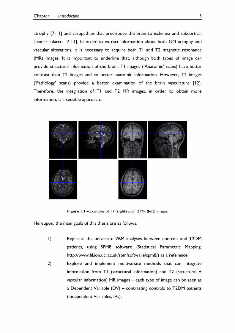
Figure 1.1 – Examples of T1 (right) and T2 MR (left) images. ................................................................................. 3
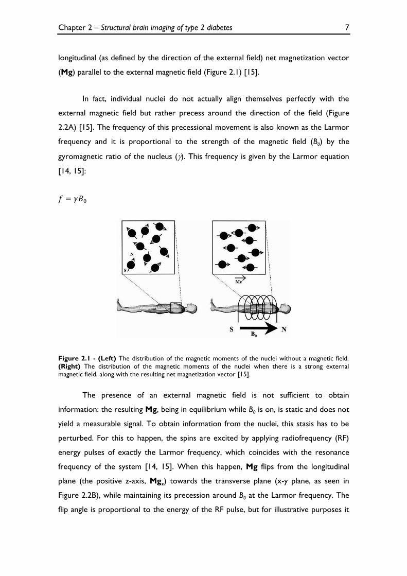
Figure 2.1 - (Left) The distribution of the magnetic moments of the nuclei without a magnetic field.
(Right) The distribution of the magnetic moments of the nuclei when there is a strong external magnetic
field, along with the resulting net magnetization vector [15]. ................................................................................. 7
Figure 2.2 - (A) The orientation of the spins in presence of an external magnetic field. (B) The net
magnetization vector (M) flips 90° from the longitudinal plane (the positive z-axis) to transverse x-y
Figure 2.3 - T1 and T2 relaxation time representation [15].................................................................................... 9
Figure 2.4 – T1 and T2 images, respectively, obtained in SPM8. .......................................................................... 11
Figure 2.5 - Spatial normalization in VBM (images obtained in SPM8). ............................................................... 13
Figure 2.6 - Segmentation in VBM (images obtained in SPM8). ............................................................................. 14
Figure 2.7 - Smoothing in VBM (images obtained in SPM8). .................................................................................. 15
Figure 3.1 - F distribution [23]....................................................................................................................................... 23
Figure 3.2 - The new design menu for the MANCOVA algorithm. ..................................................................... 30
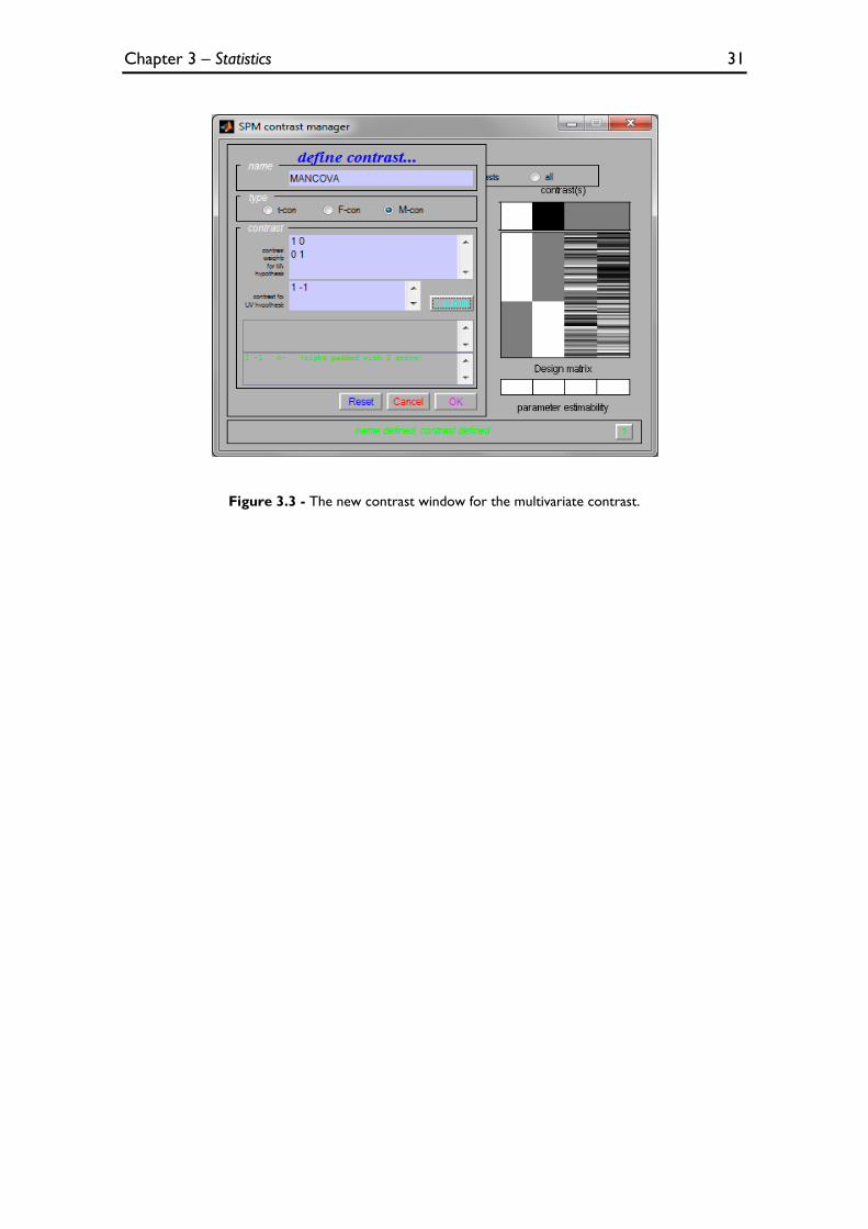
Figure 3.3 - The new contrast window for the multivariate contrast. ................................................................ 31
Figure 3.4 - The general process of classification algorithms [31]. ...................................................................... 32
Figure 3.5 - Illustration of the SVM concept in an imaginary 2D space [4]........................................................ 34
Figure 4.1 - An example of overlapping a (blue) significance map image with a high resolution image. ..... 37
Figure 4.2 - ANCOVA obtained with an in-house function in Matlab, using T1 images. ............................... 39
Figure 4.3 – The previous ANCOVA image overlaid with a high resolution image. ....................................... 39
Figure 4.4 - ANCOVA obtained in SPM8 (VBM), using T1 images. ..................................................................... 40
Figure 4.5 - ANCOVA obtained with an in-house function in Matlab, using T2 images. ............................... 41
Figure 4.6 - The previous ANCOVA image overlaid with a high resolution image. ....................................... 41
Figure 4.7 - ANCOVA obtained in SPM8 (VBM), using T2 images. ..................................................................... 42
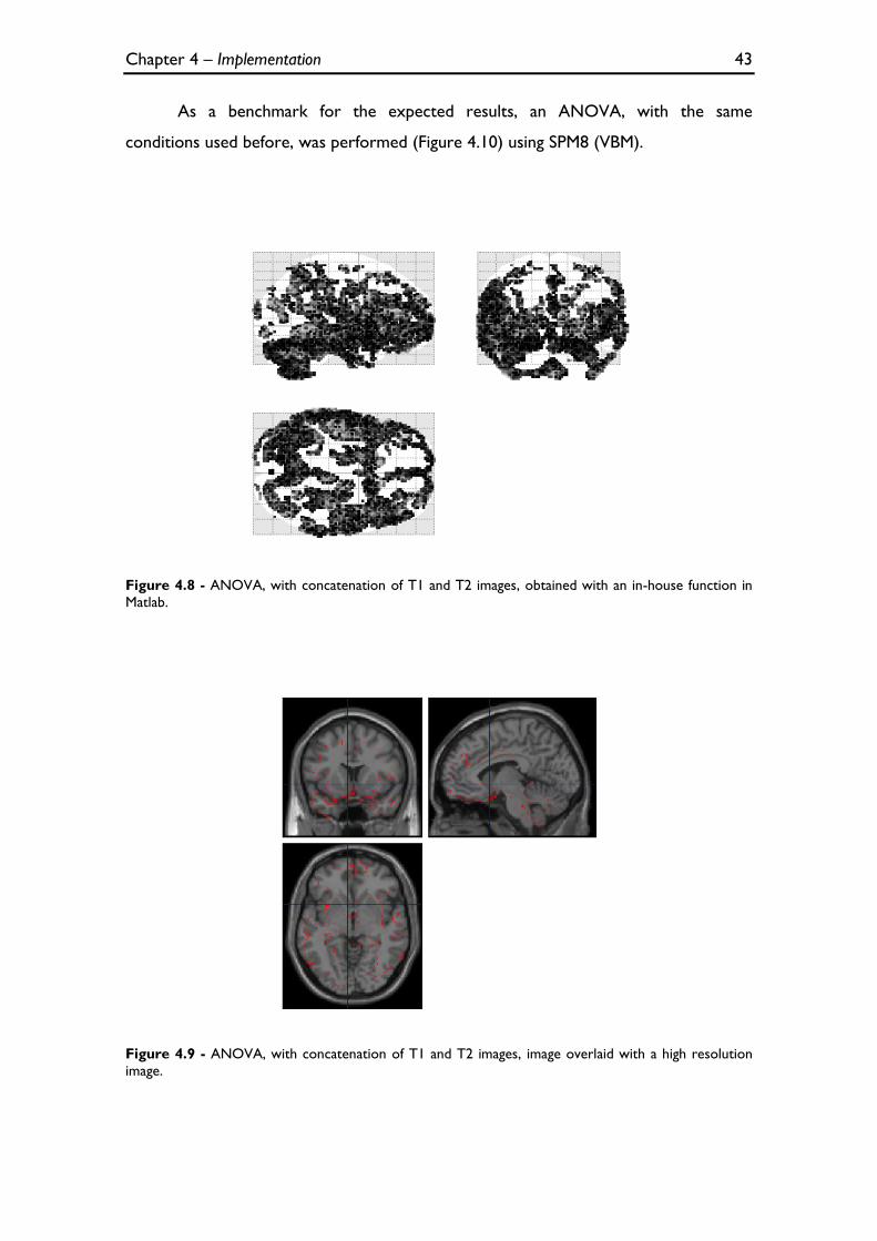
Figure 4.8 - ANOVA, with concatenation of T1 and T2 images, obtained with an in-house function in
Figure 4.13 - ANCOVA, with concatenation of T1 and T2 images, obtained in SPM8 (VBM). .................... 46
Figure 4.14 - Two-sample Hotelling's T2 obtained with an in-house function in Matlab. ............................... 48
Figure 4.15 - The previous Hotelling's T2 image overlaid with a high resolution image. ................................ 48
Figure 4.16 - MANOVA obtained with an in-house function in Matlab. ............................................................ 49
Figure 4.17 - The previous MANOVA image overlaid with a high resolution image. ..................................... 49
Figure 4.18 - MANCOVA obtained with an in-house function in Matlab. ......................................................... 50
Figure 4.19 - The previous MANCOVA image overlaid with a high resolution image. .................................. 51
Figure 4.20 - MANCOVA obtained in SPM8 (VBM). ............................................................................................... 51
Figure 4.21 – The results of the inferential multivariate methods (A - Hotelling’s T2, B - MANOVA and C
- MANCOVA), compared with a map of weights, obtained in PRoNTo software using SVM algorithm
(D), at the coordinate [-10.7 15.4 1.7] mm. .............................................................................................................. 52
xxiii
Contents
Acknowledgments ......................................................................................................... xi
Abstract ........................................................................................................................ xiii
Resumo ........................................................................................................................... xv
Symbols & Abbreviations ............................................................................................ xvii
List of Figures ............................................................................................................... xxi
4.2.1.2 ANOVA with concatenation of T1 and T2 images ........................................................... 42 4.2.1.3 ANCOVA with concatenation of T1 and T2 images ........................................................ 44
The software used to apply a classification method was the PRoNTo toolbox
(explained in the section 4.1.6) and the algorithm used was a linear SVM (with c
parameter equal to one). In order to perform a binary classification (controls versus
T2DM patients), two modalities (T1 images and T2 images) were inserted. This
allowed the simultaneously analysis of T1 and T2 images, comparing the brain
differences between the controls and T2DM subjects. In order to specify the model:
the input feature set chosen was the GM volume of each image, the kernel was the
multiplication of all images and the cross-validation method was the LOO. The
outcome is a map of weights that may be compared with the results of the inferential
multivariate methods (Figure 4.21). The sensibility and specificity of the classification
was 83.3% and 72.1%, respectively.
Figure 4.21 – The results of the inferential multivariate methods (A - Hotelling’s T2, B - MANOVA and
C - MANCOVA), compared with a map of weights, obtained in PRoNTo software using SVM algorithm
(D), at the coordinate [-10.7 15.4 1.7] mm.
Chapter 5 – Discussion & Conclusions 53
Chapter 5
Discussion & Conclusions
As stated in the introduction, this thesis had three main goals, which were
pursued in phases:
1) Replicate the univariate VBM analyses between controls and T2DM patients
in Matlab, using SPM8 software as a reference;
2) Explore and implement multivariate methods that can integrate information
from T1 and T2 images, contrasting controls to T2DM patients;
3) Insertion of these multivariate algorithms into the pipeline of SPM8 so that
it can be used in further multimodal studies.
All these goals were successfully accomplished, as further expanded below.
5.1 Univariate Analyses and Type 2 Diabetes Mellitus
In the first phase, the standard GLM algorithm used in SPM8 was coded, making
it possible to perform an ANCOVA, using only T1 or T2 images, and ANOVA and
ANCOVA with concatenation of T1 and T2 images. In both univariate analyses, the
results obtained with the replicated algorithm were identical to the results obtained
with the standard SPM8 version used for VBM (see sections 4.2.1.1, 4.2.1.2 and
4.2.1.3).
In ANCOVA for separate analysis of T1 and T2 images, the structural and
vascular changes are clearly visible in T1 and T2 images, respectively, and they are
more noticeable in the limbic lobe, sub-lobar, insular and temporal areas (brain areas
Chapter 5 – Discussion & Conclusions 54
responsible for emotional and cognitive functions), bilaterally. These results are in
agreement with the expected brain alterations in T2DM patients, described in the
literature [7-11]. Furthermore, other publications corroborate these results: in a study
where a relatively large population (350 patients and 364 controls) was used, a pattern
of GM loss was found mainly in the medial temporal, anterior cingulated and medial
frontal lobes [36]; and in a recent study where similar changes, particularly in the
limbic system and temporo-parietal lobes (cingulum, insular area, hippocampus) are
described [37].
The results of the ANOVA with the concatenation of T1 and T2 images were
not as specific (see section 4.2.1.2) because the exclusion of the nuisance covariates
from the analysis leads to more ‘noise’ in the images. In order to surpass this
limitation, the script was altered and the insertion of the covariates was performed
(see section 4.2.1.3). These results are comparable with the results of the ANCOVA
analyses using T1 and T2 images separately (section 4.2.1.1), i.e. the atrophic tissue is
also predominant in the limbic lobe, sub-lobar, insular and temporal areas.
5.2 Multivariate Analyses and Type 2 Diabetes Mellitus
In the second phase, three inferential multivariate methods were implemented
(Hotelling’s T2, MANOVA and MANCOVA). Although the results of these analyses
seem different, they are identical, but as MANOVA and Hotelling’s methods do not
presuppose the insertion of the nuisance covariates and MANCOVA does, the latter
may lead to ‘cleaner’ results, i.e. more specific results, with less false positives.
Nevertheless, the differences in cortical tissue are also visible in the three
analyses, being more noticeable in the limbic lobe, sub-lobar, insular and temporal
areas as well (see sections 4.2.2.1.1, 4.2.2.1.2 and 4.2.2.1.3). Though the univariate
analyses lead to clinically sensible results, the multivariate analyses may lead to more
powerful results without a loss of specificity: in fact, the atrophic brain areas detected
seem more restricted (e.g. compare the MANOVA versus ANOVA results and
MANCOVA e ANCOVA results). It is worth underlining that multivariate analyses
Chapter 5 – Discussion & Conclusions 55
allow for the assessment of data from different “views”, providing greater
discriminative power, which may lead to enhanced inference.
It cannot be excluded, however, that the correlation between T1 and T2 (both
DVs used herein) may have pose a hindrance to the application of the multivariate
methods: this is a key limitation of this work; indeed, it must be acknowledged that a
number of presuppositions that should have been in place to ensure the validity of the
application of these parametric multivariate tests – apart from the normality of the
data, which was ensure through spatial smoothing – were not tested. This is, however,
not critical in this “proof of concept” (PoC) stage, but will be required in future work.
After that, these multivariate results were compared with a single SVM result
(Figure 4.21). Instead a map of significance, the latter result is a map of weight
coefficients. It is possible to perceive the brain differences between control subjects
and T2DM subjects: in this case, the red regions can be interpreted, though not with
full certainty, as regions where the GM volume is greater in controls than T2DM
patients. Seen from this perspective, this map is somewhat similar to the other maps
obtained with the inferential multivariate methods, especially with Hotelling’s T2 and
MANOVA – this may be so because the nuisance covariates were not introduced in
the SVM data (Figure 4.21).
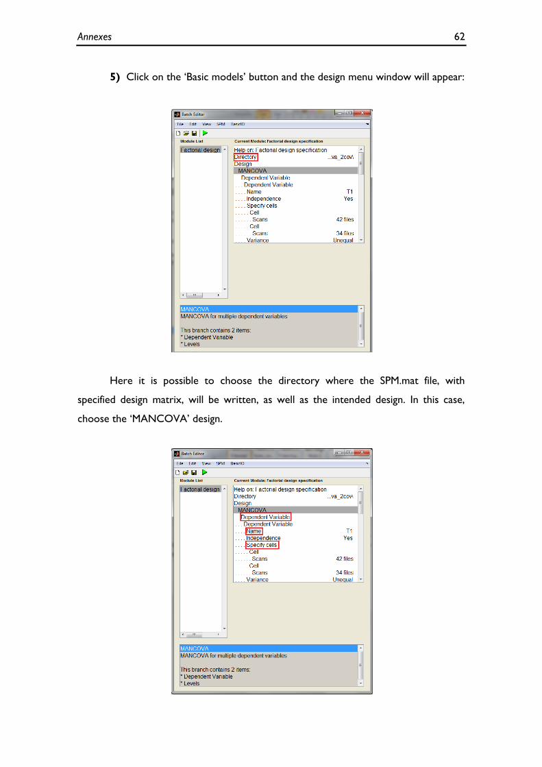
5.3 Possible Future SPM8 toolbox
In the last phase, in which proved to be the most challenging aspect of this
thesis, the alterations in the SPM8 functions, mentioned in the section 3.2.2.4, were
implemented, notably the creation of the design menu and the contrast window. With
all of these alterations, the MANCOVA algorithm was fully inserted in SPM8 and the
first multivariate result within this software (Figure 4.20) was obtained. This thesis is
the groundwork for a publicly available multivariate statistics toolbox, to be inserted in
this widely used brain imaging platform.
Chapter 5 – Discussion & Conclusions 56
5.4 Limitations & Future work
It is crucial understand that this work is a “proof of concept”, i.e. the main
objective of this thesis is not create a perfect algorithm to prove the brain alterations
in T2DM, but demonstrate that it is possible to implement inferential multivariate
methods in an accessible programming language (Matlab) while inserting these
algorithms in a toolbox for a widely used brain imaging platform such as SPM8. As
mentioned before, given time and data constraints, volumetric T1 and T2 brain scans
obtained from subjects who participated in the Diamarker project were used. The
implementation was adapted to these limited data, not taking into account difficulties
that may arise from using multiple modalities (e.g. PET and fMRI), notably different scan
space and resolution.
Additionally, as mentioned above, some of the pre-requisites to perform
statistical tests were not tested, notably the correlation between DVs. Future work
will focus on surpassing these limitations and preparing the methods to be applied in
multimodal studies.
References 57
References
1. Aine, C.J., A conceptual overview and critique of functional neuroimaging techniques in humans: I. MRI/FMRI and PET. Crit Rev Neurobiol, 1995. 9(2-3): p. 229-309.
2. Luo, W.L. and T.E. Nichols, Diagnosis and exploration of massively univariate neuroimaging models. Neuroimage, 2003. 19(3): p. 1014-32.
3. Friston, K.J., Statistical parametric maps in functional imaging: A General Linear Approach. Human Brain Mapping, 1995. 2: p. 189-210.
4. Gaonkar, B. and C. Davatzikos, Analytic estimation of statistical significance maps for support vector machine based multi-variate image analysis and classification. Neuroimage, 2013. 78: p. 270-83.
5. Liu, F., et al., Inter-modality relationship constrained multi-modality multi-task feature selection for Alzheimer's Disease and mild cognitive impairment identification. Neuroimage, 2014. 84: p. 466-75.
6. Duarte, J.V., et al., Multivariate pattern analysis reveals subtle brain anomalies relevant to the cognitive phenotype in neurofibromatosis type 1. Human Brain Mapping, 2014. 35(1): p. 89-106.
7. Guerrero-Berroa, E., J. Schmeidler, and M.S. Beeri, Neuropathology of type 2 diabetes: a short review on insulin-related mechanisms. Eur Neuropsychopharmacol, 2014.
8. Wrighten, S.A., et al., A look inside the diabetic brain: Contributors to diabetes-induced brain aging. Biochim Biophys Acta, 2009. 1792(5): p. 444-453.
9. van Harten, B., et al., Brain lesions on MRI in elderly patients with type 2 diabetes mellitus. Eur Neurol, 2007. 57(2): p. 70-4.
10. Manschot, S.M., et al., Brain magnetic resonance imaging correlates of impaired cognition in patients with type 2 diabetes. Diabetes, 2006. 55(4): p. 1106-13.
11. den Heijer, T., et al., Type 2 diabetes and atrophy of medial temporal lobe structures on brain MRI. Diabetologia, 2003. 46(12): p. 1604-10.
References 58
12. MacDonald-Jankowski, D.S., Magnetic Resonance Imaging. Part 1: the Basic Principles. Asian Journal of Oral and Maxillofacial Surgery, 2006. 18(3): p. 165-171.
13. Glassman, N.R., Magnetic Resonance Imaging. Journal of Consumer Health On the Internet, 2010. 14(3): p. 308-321.
14. Sands, M.J. and A. Levitin, Basics of magnetic resonance imaging. Seminars in Vascular Surgery, 2004. 17(2): p. 66-82.
15. van Geuns, R.-J.M., et al., Basic Principles of Magnetic Resonance Imaging. Progress in Cardiovascular Diseases 1999. 42(2): p. 149-156.
16. Ashburner, J. and K.J. Friston, Voxel-based morphometry--the methods. Neuroimage, 2000. 11(6 Pt 1): p. 805-21.
17. Mechelli, A., et al., Voxel-Based Morphometry of the Human Brain: Methods and Applications. Current Medical Imaging Reviews 2005. 1(1).
18. Ashburner, J. and K.J. Friston, Unified segmentation. Neuroimage, 2005. 26(3): p. 839-51.
19. Timm, N.H., Applied multivariate analysis. 2002, New York: Springer
20. Friston, K.J., et al., Human Brain Function. 2nd ed. 2004, San Diego, California: Academic Press.
21. Tabachnick, B.G. and L.S. Fidell, Using Multivariate Statistics 5th ed. 2007, Boston: Pearson.
22. Datalo, P., Analysis of Multiple Dependent Variables. 1st ed. 2013, New York: Oxford University Press.
23. Statistical Tables: F distribution [Online]. Available from: http://www.philender.com/courses/tables/dist3.html.
24. The General Linear Model (GLM) [Online]. Available from: http://support.brainvoyager.com/functional-analysis-statistics/35-glm-modelling-a-single-study/82-users-guide-the-general-linear-model.html.
25. Şenoğlu, B., Estimating parameters in one-way analysis of covariance model with short-tailed symmetric error distributions. Journal of Computational and Applied Mathematics, 2007. 201(1): p. 275-283.
26. Flury, B., A First Course in Multivariate Statistics. 1st ed. 1997, New York: Springer.
27. Rencher, A.C., Methods of Multivariate Analysis. 2nd ed. 2002, New York: John Wiley & Sons, Inc.
28. Hofacker, C.F., Mathematical Marketing. 2007: New South Network Services.
29. The Two-Sample Hotelling's T-Square Test Statistic [Online]. Available from: https://onlinecourses.science.psu.edu/stat505/node/124.
30. Illán, I.A., et al., Computer aided diagnosis of Alzheimer’s disease using
component based SVM. Applied Soft Computing, 2011. 11(2): p. 2376-2382.
31. Pereira, F., T. Mitchell, and M. Botvinick, Machine learning classifiers and fMRI: a tutorial overview. Neuroimage, 2009. 45(1 Suppl): p. S199-209.
32. Alberti, K.G. and P.Z. Zimmet, Definition, diagnosis and classification of diabetes mellitus and its complications. Part 1: diagnosis and classification of diabetes mellitus provisional report of a WHO consultation. Diabet Med, 1998. 15(7): p. 539-53.
33. Definition and Diagnosis of Diabetes Mellitus and Intermediate Hyperglycemia. 2011: World Health Organization.
34. Schrouff, J., et al., PRoNTo: pattern recognition for neuroimaging toolbox. Neuroinformatics, 2013. 11(3): p. 319-37.
35. PRoNTo Manual [Online]. Available from: http://www.mlnl.cs.ucl.ac.uk/pronto/prt_manual.pdf.
36. Moran, C., et al., Brain atrophy in type 2 diabetes: regional distribution and influence on cognition. Diabetes Care, 2013. 36(12): p. 4036-42.
37. Cui, X., et al., Multi-scale glycemic variability: a link to gray matter atrophy and cognitive decline in type 2 diabetes. PLoS One, 2014. 9(1): p. e86284.