FDR and Bayesian Multiple Comparisons Rulesbrad/7440/MuellerParmigianiRice… · · 2008-12-22FDR...

Johns Hopkins UniversityJohns Hopkins University, Dept. of Biostatistics Working Papers

Year Paper

FDR and Bayesian Multiple ComparisonsRules

Peter Muller∗ Giovanni Parmigiani†

Kenneth Rice‡

∗M.D. Anderson Cancer Center†The Sydney Kimmel Comprehensive Cancer Center, Johns Hopkins University & Department

of Biostatistics, Johns Hopkins Bloomberg School of Public Health, [email protected]‡University of Washington

This working paper is hosted by The Berkeley Electronic Press (bepress) and may not be commer-cially reproduced without the permission of the copyright holder.

http://www.bepress.com/jhubiostat/paper115

Copyright c©2006 by the authors.


Peter Muller, Giovanni Parmigiani, and Kenneth Rice

Abstract

We discuss Bayesian approaches to multiple comparison problems, using a de-cision theoretic perspective to critically compare competing approaches. We setup decision problems that lead to the use of FDR-based rules and generalizations.Alternative definitions of the probability model and the utility function lead to dif-ferent rules and problem-specific adjustments. Using a loss function that controlsrealized FDR we derive an optimal Bayes rule that is a variation of the Benjaminiand Hochberg (1995) procedure. The cutoff is based on increments in orderedposterior probabilities instead of ordered p- values. Throughout the discussionwe take a Bayesian perspective. In particular, we focus on conditional expectedFDR, conditional on the data. Variations of the probability model include explicitmodeling for dependence. Variations of the utility function include weighting bythe extent of a true negative and accounting for the impact in the final decision.

Proc. Valencia / ISBA 8th World Meeting on Bayesian StatisticsBenidorm (Alicante, Spain), June 1st–6th, 2006


Peter Muller, Giovanni Parmigiani & Kenneth RiceM.D. Anderson Cancer Center, USA Johns Hopkins University, USA

University of Washington, Seattle, USA

[email protected] [email protected] [email protected]

Summary

We discuss Bayesian approaches to multiple comparison problems, using adecision theoretic perspective to critically compare competing approaches.We set up decision problems that lead to the use of FDR-based rules andgeneralizations. Alternative definitions of the probability model and the utilityfunction lead to different rules and problem-specific adjustments. Using a lossfunction that controls realized FDR we derive an optimal Bayes rule that is avariation of the Benjamini and Hochberg (1995) procedure. The cutoff is basedon increments in ordered posterior probabilities instead of ordered p-values.Throughout the discussion we take a Bayesian perspective. In particular, wefocus on conditional expected FDR, conditional on the data. Variations ofthe probability model include explicit modeling for dependence. Variationsof the utility function include weighting by the extent of a true negative andaccounting for the impact in the final decision.

Keywords and Phrases: Decision problems; Multiplicities; Falsediscovery rate.

1. INTRODUCTION

We discuss Bayesian approaches to multiple comparison problems, using a Bayesiandecision theoretic perspective to critically compare competing approaches. Multi-ple comparison problems arise in a wide variety of research areas. Many recentdiscussions are specific to massive multiple comparisons arising in the analysis ofhigh throughput gene expression data. See, for example, Storey et al. (2004) andreferences therein. The basic setup is a large set of comparisons. Let ri denote theunknown truth in the i-th comparison, ri = 0 (H0) versus ri = 1 (H1), i = 1, . . . , n.In the context of gene expression data a typical setup defines ri as an indicator forgene i being differentially expressed under two biologic conditions of interest. Foreach gene a suitably defined difference score zi is observed, with zi ∼ f0(zi) if ri = 0,and zi ∼ f1(zi) if ri = 1. This is the basic setup of the discussions in Benjamini andHochberg (1995); Efron et al. (2001); Storey (2002); Efron and Tibshirani (2002);Genovese and Wasserman (2002, 2003); Storey et al. (2004); Newton et al. (2004);Cohen and Sackrowitz (2005) and many others. A traditional approach to address

Hosted by The Berkeley Electronic Press

2 Muller, Parmigiani & Rice

the multiple comparison problem in these applications is based on controlling falsediscovery rates (FDR), the proportion of false rejections relative to the total num-ber of rejections. We discuss details below. A similar setup arises in the analysisof high throughput protein expression data, for example, mass/charge spectra fromMALDI-TOF experiments, as described in Baggerly et al. (2003).

Many other applications lead to similar massive multiple comparison problems.Clinical trials usually record data for an extensive list of adverse events (AE). Com-paring treatments on the basis of AEs takes the form of a massive multiple compari-son problem. Berry and Berry (2004) argue that the hierarchical nature of AEs, withAEs grouped into biologically different body systems, is critical for an appropriateanalysis of the problem. Another interesting application of multiple comparisonand FDR is in classifying regions in image data. Genovese et al. (2002) proposean FDR-based method for threshold selection in neuroimaging. Shen et al. (2002)propose an enhanced procedure that takes into account spatial dependence, specifi-cally in a wavelet based spatial model. Another traditional application of multiplecomparisons arises in record linkage problems. Consider two data sets, A and B,for example billing data and clinical data in a clinical trial. The record matchingproblem refers to the question of matching data records in A and B correspondingto the same person. Consider a partition of all possible pairs of data records in Aand B into matches versus non-matches. A traditional summary of a given parti-tion is the Correct Match Rate (CMR), defined as the fraction of correctly guessedmatches relative to the number of true matches. See, for example, Fortini et al.(2001, 2002). Another interesting related class of problems are ranking and selec-tion problems. Lin et al. (2004) describe the problem of constructing league tables,i.e., reporting inference on ranking a set of units (hospitals, schools, etc.). Lin et al.explicitly acknowledge the nature of the multiple comparison as a decision problemand discuss solutions under several alternative loss functions.

To simplify the remaining discussion we will assume that the multiple compari-son problem arises in a microarray group comparison experiment, keeping in mindthat the discussion remains valid for many other massive multiple comparison. Amicroarray group comparison experiment records gene expression for a large num-ber of genes, i = 1, . . . , n, under two biologic conditions of interest, for exampletumor tissue and normal tissue. For each gene we are interested in the comparisonof the two competing hypotheses that gene i is differentially expressed versus notdifferentially expressed. We will refer to a decision to report a gene as differentiallyexpressed as a discovery (or positive, or rejection), and the opposite as a negative(fail to reject).

2. FALSE DISCOVERY RATES

Many recently proposed approaches to address massively multiple comparisons arebased on controlling false discovery rates (FDR), introduced by Benjamini andHochberg (1995). Let δi denote an indicator for rejecting the i-th comparison,for example flagging gene i as differentially expressed and let D =

Pδi denote the

number of rejections. Let ri ∈ {0, 1} denote the unknown truth, for example an in-dicator for true differential expression of gene i. We define FDR = (

P(1− ri)δi)/D

as the fraction of false rejections, relative to the total number of rejections. Theratio defines a summary of the parameters (ri), the decisions (δi) and the data (in-directly, through the decisions). As such it is neither Bayesian nor frequentist. Howwe proceed to estimate and/or control it depends on the chosen paradigm. Tradi-tionally one considers the (frequentist) expectation E(FDR), taking an expectation


Bayesian Multiple Comparisons 3

over repeated experiments. This is the definition used in Benjamini and Hochberg(1995). Applications of FDR to microarray analysis are discussed, among manyothers, in Efron and Tibshirani (2002). Storey (2002, 2003) introduces the pos-itive FDR (pFDR) and the q-value and improved estimators for the FDR. In thepFDR the expectation is defined conditional on D > 0. Efron and Tibshirani (2002)show the connection between FDR and the empirical Bayes procedure proposed inEfron et al. (2001) and the FDR control as introduced in Benjamini and Hochberg(1995). Genovese and Wasserman (2003) discuss more cases of Bayes-frequentistagreement in controlling various aspects of FDR. Let pi denote a p-value for testingri = 1 versus ri = 0. They consider rules of the type δi = I(pi < t). Controllingthe posterior probability P (ri = 0 | Y, pi = t) is stronger than controlling the ex-pected FDR for a threshold t. Specifically, let FDR(t) denote FDR under the ruleδi = (pi < t), let q(t) ≈ P (ri = 0 | Y, pi = t) denote an approximate evaluation ofthe posterior probability for the i−th comparison, and let Q(t) ≈ E(FDR(t)) denotean asymptotic approximation of expected FDR. Then q(t) ≤ Q(t). The argumentassumes concavity of the c.d.f. for p-values under the alternative ri = 1. Genoveseand Wasserman (2002) also show an agreement of confidence intervals and crediblesets for FDR. They define the realized FDR process FDR(T ) as a function of thethreshold T and call T a (c, α) confidence threshold if P (FDR(T ) < c) ≥ 1−α. Theprobability is with respect to a sampling model that includes an (unknown) mixtureof true and false hypotheses. The Bayesian equivalent is a posterior credible set,i.e., controlling P (FDR(T ) ≤ c | Y ) ≤ 1 − α. Genovese and Wasserman (2003)show that controlling the posterior credible interval for FDR(T ) is asymptoticallyequivalent to controlling the confidence threshold.

Let zi denote some univariate summary statistic for the i-th comparison, forexample a p-value. Many discussions are in the context of an assumed i.i.d. samplingmodel for zi, from a mixture model f(·) with terms f0 and f1 corresponding tosubpopulations of differentially and not-differentially expressed genes, respectively:

zi ∼ p0 f0(zi) + (1− p0) f1(zi) ≡ f(zi).

Using latent indicators ri ∈ {0, 1} introduced earlier, the mixture is equivalent tothe hierarchical model:

p(zi | ri = j) = fj(zi) and Pr(ri = 0) = p0 (1)

Let F0 and F denote the c.d.f. for f0 and f . Efron and Tibshirani (2002) defineFDR for rejection regions of the type {zi ≤ z},

Fdr(z) ≡ p0F0(z)/F (z)

and denote it “Bayesian FDR”. The Bayesian label is justified by the use of Bayestheorem to find the probability of false discovery given {zi ≤ z}, which they show isequivalent to the defined Fdr statistic. The probability statement is in the context ofthe assumed mixture model, for assumed known f0, f1 and p0. In particular, there isno learning about p0. However, using reasonable data-driven point estimates for theunknown quantities f0, f1 and p0, the Fdr statistic provides an good approximationfor what P (rn+1 = 1 | zn+1 ≤ z, Y ) would be in a full Bayesian model with flexiblepriors on f1 and f0. Here and throughout this paper we use Y to generically indicatethe observed data. Efron et al. (2001) introduce local FDR, as

fdr(z) ≡ p0f0(z)/f(z).



Under the mixture model, and conditioning on f0, f1 and p0, the fdr statistic is theprobability of differential expression, so fdr(z) = Pr(ri = 1 | zi = z, Y, f0, f1, p0).As before, one can argue that under a sufficiently flexible prior probability model onf0, f1, p0, reasonable point estimates can be substituted for the unknown quantities,allowing us to interpret values of fdr as posterior probabilities, without reference to aspecific prior model (subject to identifiability constraints). In the following sectionswe argue that posterior inference for the multiple comparison should consider morestructured models. Inference should not stop with the marginal posterior probabilityof differential expression. Rules of the type δi = I(zi ≤ z) are intuitive, but notnecessarily optimal. In the context of a full probability model, and assuming areasonable utility function, it is straightforward to derive the optimal rule.

Considering frequentist expectations of FDR, i.e., expectations over repeatedsampling, we need to consider expectations over a ratio of random variables. Shortof uninteresting trivial decision rules, the decision δi = δi(Y ) is a function of thedata and appears in both, numerator and denominator of the ratio. The discussionsignificantly simplifies under a Bayesian perspective. The only unknown quantity inFDR =

Pδi(1− ri)/D is the unknown ri in the numerator. Let vi = P (ri = 1 | Y )

denote the marginal posterior probability of gene i being differentially expressedand define

FDR = E(FDR | Y ) =X

(1− vi)δi/D. (2)

Newton et al. (2004) consider decision rules that classify a gene as differentiallyexpressed if vi > γ∗, fixing γ∗ to achieve a certain pre-set false discovery rate,FDR ≤ α. Newton et al. (2004) comment on the dual role of vi in decision rules likeδi = I(vi > γ∗). It determines the decision, and at the same time already reportsthe probability of a false discovery as 1− vi for δi = 1 and the probability of a falsenegative as vi for δi = 0.

3. POSTERIOR PROBABILITIES ADJUST FOR MULTIPLICITIES

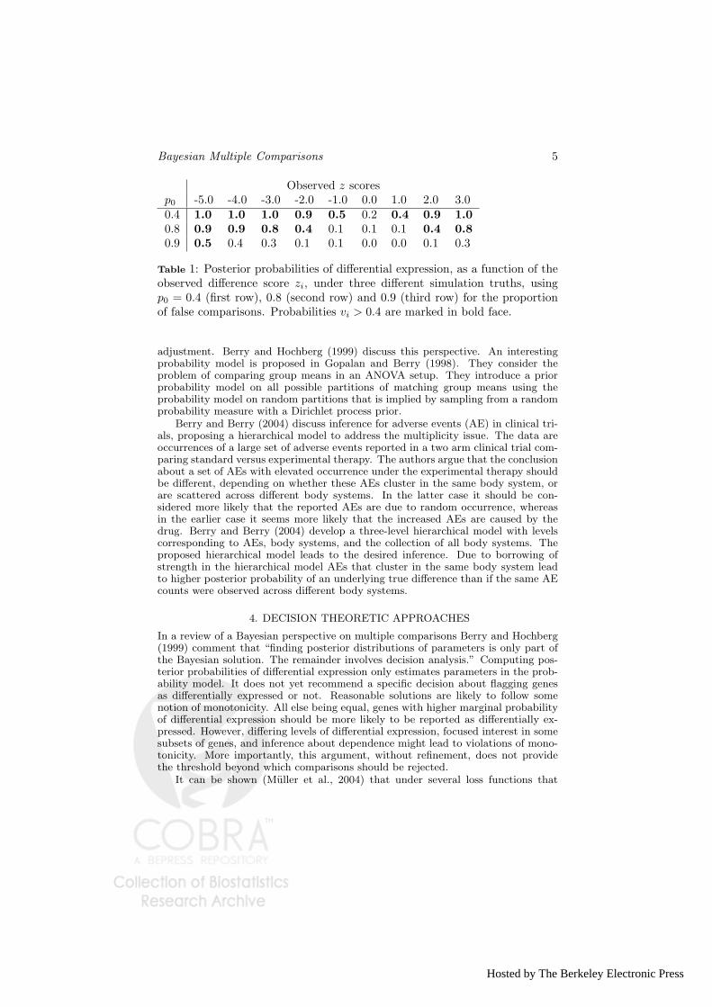
“Posterior inference adjusts for multiplicities, and no further adjustment is re-quired.” The statement is only true with several caveats. First, the probabilitymodel needs to include a positive prior probability of non-differential expression foreach gene i. Second, the model needs to include a hyperparameter that defines theprior probability mass for non-differential expression. For example, consider themixture model (1), with independence across i, conditional on p0. The statementrequires that p0 be a parameter with a hyperprior p(p0), rather than fixed. Scottand Berger (2003) discuss the nature of this adjustment and show some examples.In the context of microarray data analysis, Do et al. (2005) carry out the same sim-ulation experiment in the context of a mixture model as in (1). Results are shownin Table 1. The table shows marginal posterior probabilities vi for differential ex-pression. The nature of the model is such that vi depends on the gene only throughan observed difference score zi, making it meaningful to list vi by observed differ-ence score zi. The marginal posterior probability of differential expression adjustsfor the multiplicities. If there are many truly negative comparisons, as in the thirdrow of the table, then the model reduces the marginal probabilities of differentialexpression. If on the other hand there are many truly positive comparisons, as inthe first row, then the model appropriately increases the marginal probabilities.

The probability model need not be i.i.d. sampling. Any probability model thatincludes a positive prior probability for ri = 0 and ri = 1, i.e., any model that allowsinference on how comparisons between units are true or false leads to a similar



Observed z scoresp0 -5.0 -4.0 -3.0 -2.0 -1.0 0.0 1.0 2.0 3.00.4 1.0 1.0 1.0 0.9 0.5 0.2 0.4 0.9 1.00.8 0.9 0.9 0.8 0.4 0.1 0.1 0.1 0.4 0.80.9 0.5 0.4 0.3 0.1 0.1 0.0 0.0 0.1 0.3

Table 1: Posterior probabilities of differential expression, as a function of theobserved difference score zi, under three different simulation truths, usingp0 = 0.4 (first row), 0.8 (second row) and 0.9 (third row) for the proportionof false comparisons. Probabilities vi > 0.4 are marked in bold face.

adjustment. Berry and Hochberg (1999) discuss this perspective. An interestingprobability model is proposed in Gopalan and Berry (1998). They consider theproblem of comparing group means in an ANOVA setup. They introduce a priorprobability model on all possible partitions of matching group means using theprobability model on random partitions that is implied by sampling from a randomprobability measure with a Dirichlet process prior.

Berry and Berry (2004) discuss inference for adverse events (AE) in clinical tri-als, proposing a hierarchical model to address the multiplicity issue. The data areoccurrences of a large set of adverse events reported in a two arm clinical trial com-paring standard versus experimental therapy. The authors argue that the conclusionabout a set of AEs with elevated occurrence under the experimental therapy shouldbe different, depending on whether these AEs cluster in the same body system, orare scattered across different body systems. In the latter case it should be con-sidered more likely that the reported AEs are due to random occurrence, whereasin the earlier case it seems more likely that the increased AEs are caused by thedrug. Berry and Berry (2004) develop a three-level hierarchical model with levelscorresponding to AEs, body systems, and the collection of all body systems. Theproposed hierarchical model leads to the desired inference. Due to borrowing ofstrength in the hierarchical model AEs that cluster in the same body system leadto higher posterior probability of an underlying true difference than if the same AEcounts were observed across different body systems.

4. DECISION THEORETIC APPROACHES

In a review of a Bayesian perspective on multiple comparisons Berry and Hochberg(1999) comment that “finding posterior distributions of parameters is only part ofthe Bayesian solution. The remainder involves decision analysis.” Computing pos-terior probabilities of differential expression only estimates parameters in the prob-ability model. It does not yet recommend a specific decision about flagging genesas differentially expressed or not. Reasonable solutions are likely to follow somenotion of monotonicity. All else being equal, genes with higher marginal probabilityof differential expression should be more likely to be reported as differentially ex-pressed. However, differing levels of differential expression, focused interest in somesubsets of genes, and inference about dependence might lead to violations of mono-tonicity. More importantly, this argument, without refinement, does not providethe threshold beyond which comparisons should be rejected.

It can be shown (Muller et al., 2004) that under several loss functions that



combine false negative and false discovery counts and/or rates the optimal decisionrule is of the following form. Recall that δi is an indicator for the decision to reportgene i as differentially expressed and vi = Pr(ri = 1 | Y ) denotes the marginalposterior probability of differential expression for gene i. The optimal decision isto declare all genes with marginal probability beyond a threshold as differentiallyexpressed:

δ∗i = I(vi > t). (3)

The choice of loss function determines the specific threshold. In Muller et al. (2004)we consider four alternative loss functions. Similar to FDR we define FD =

P(1−

ri)δi and FN =P

ri(1 − δi) as the false positive and false negative counts, and

FNR = FN/(n − D) as the false negative ratio. We use FD, FN and FNR for

the posterior expectations. All are easily evaluated. For example, FN =P

vi(1 −δi). Considering various combinations of these statistics we define alternative lossfunctions. Since the posterior expectation is straightforward, we specify the lossfunctions already as posterior expected loss. The first two loss functions are linearcombinations of the false negative and positive counts and ratios. We define

LN (δ, z) = c FD + FN, (4)

and LR(δ, z) = c FDR + FNR. The loss function LN is a natural extension of(0, 1, c) loss functions for traditional hypothesis testing problems (Lindley, 1971).From this perspective the combination of error rates in LR seems less attractive.The loss for a false discovery and false negative depends on the total number ofdiscoveries or negatives, respectively. Genovese and Wasserman (2002) interpret cas the Lagrange multiplier in the problem of minimizing FNR subject to a bound onFDR. They compare the Benjamini and Hochberg (1995) rule (BH) and the optimalrule under LR and show that BH almost achieves the optimal risk, in particular fora large fraction of true nulls.

Alternatively, we consider bivariate loss functions that explicitly acknowledgethe two competing goals:

L2R(δ, z) = (FDR, FNR), L2N (δ, z) = (FD, FN).

We need to define the minimization of the bivariate functions. A traditional ap-proach to select an action in multicriteria decision problems is to minimize onedimension of the loss function while enforcing a constraint on the other dimensions(Keeney et al., 1976). We thus define the optimal decisions under L2N as the mini-

mization of FN subject to FD ≤ αN . Similarly, under L2R we minimize FNR subjectto FDR ≤ αR.

Under all four loss functions the optimal rule is of the form (3). See Muller et al.(2004) for a statement of the optimal cutoffs t. The result is true for any probabilitymodel with non-zero prior probability for differential and non-differential expression.In particular, the probability model could include dependence across genes.

One of the assumptions underlying these loss functions is that all false negativesare equally undesirable, and all false positives are equally undesirable. This is inap-propriate in most applications. A false negative for a gene that is truly differentiallyexpressed, but with a small difference across the two biologic conditions, is surelyless of a concern than a false negative for a gene that is differentially expressed witha large difference. The large difference might make it more likely that follow upexperiments will lead to significant results. Assume now that the probability model



includes for each gene i a parameter mi that can be interpreted as the level of dif-ferential expression, with mi = 0 if ri = 0, and mi > 0 if ri = 1. For example, inthe hierarchical gamma/gamma model proposed in Newton et al. (2001) this couldbe the absolute value of the log ratio of the gamma scale parameters that indexthe sampling distributions under the two biologic conditions. A log ratio of mi = 0implies equal sampling distributions, i.e., no differential expression. In the mixtureof Dirichlet process model of Do et al. (2005), mi would be the absolute value ofthe latent variable generated from the random probability measure with Dirichletprocess prior. A natural extension of the earlier loss functions is to

Lm(m, δ, z) = −X

δi mi + kX

(1− δi)mi + c D.

A similar weighting with the relative magnitude of errors is underlying Duncan’s(1965) multiple comparison procedure. Since ri = 0 implies m = 0, the summationsgo only over all true positives, ri = 1. The loss function includes a reward propor-tional to mi for a correct discovery, and a penalty proportional to mi for each falsenegative. The last term encourages parsimony, without which the optimal decisionwould be to trivially flag all genes. Straightforward algebra shows that the optimaldecision is similar to (3). Let mi = E(mi | Y ) denote the posterior expected levelof differential expression for gene i. The optimal rule is

δ∗i = I{mi ≥ c/(1 + k)} :

Flag all genes with mi greater than a fixed cutoff. The optimal rule remains essen-tially the same if we replace mi in the loss function by some function of m, allowingin particular for the loss to be a non-linear function of the true level of differentialexpression.

Lf (m, δ, z) = −X

δifD(mi) +X

(1− δi)fN (mi) + c D. (5)

The functions fD(m) and fN (m) would naturally be S-shaped, monotone functions

with a minimum at m = 0, and perhaps level off for large levels of m. Let fN i =

E(fN (m) | Y ) denote the posterior expectation for fN (mi), and similarly for fD.The optimal decision is

δ∗f = I{fDi + kfN i > c}.

Flag all genes with sufficiently large expected reward for discovery and/or penaltyfor a false negative. The rule δ∗f follows from the fact that the choice of mi in Lm

was arbitrary.The introduced loss functions are all generic in the sense of being reasonable loss

functions without reference to a specific decision related to the multiple comparisons.If the goal of the inference is a very specific decision with a clearly recognizableimplication, a problem-specific loss function should be used as the relevant criterionfor the multiple comparison. For example, Lin et al. (2004) and Shen and Louis(1998) consider the problem of ranking units like health care providers. Rankingis a specific form of a multiple comparison problem. It could be described as allpairwise comparisons, subject to transitivity. They introduce loss functions thatformalize the implications of a specific ranking, relative to the true ranks, and showthe optimal rules for several such loss functions.



Example 1: Epithelial Ovarian Cancer (EOC)

Wang et al. (2004) report a study of epithelial ovarian cancer (EOC). The goalof the study is to characterize the role of the tumor microenvironment in EOC.To this end the investigators collected tissue samples from patients with benignand malignant ovarian pathology. Specimens were collected, among other sites,from peritoneum adjacent to the primary tumor. RNA was co-hybridized withreference RNA to a custom-made cDNA microarray including a combination of theResearch Genetics RG HsKG 031901 8k clone set and 9,000 clones selected fromRG Hs seq ver 070700. A complete list of genes is available at

http://nciarray.nci.nih.gov/gal files/index.shtml(The array is listed as custom printing Hs-CCDTM-17.5k-1px).

We focus on the comparison of 10 peritoneal samples from patients with benignovarian pathology versus 14 samples from patients with malignant ovarian pathol-ogy. The raw data was pre-processed using BRB ArrayTool(http://linus.nci.nih.gov/BRB-ArrayTools.html). In particular, spots with min-imum intensity less than 300 in both fluorescence channels were excluded from fur-ther analysis. See Wang et al. (2004) for a detailed description.

We computed probabilities of differential expression using the POE model pro-posed in Parmigiani et al. (2002). Inference is summarized by marginal probabilitiesof differential expression vi. One parameter in the model is interpretable as the levelof differential expression. Briefly, the basic POE model includes a trinary indicatoreit for gene i and sample t, with eit ∈ {−1, 0, 1} for under-expression, normal andover-expression. In a variation of the original POE model we use a probit priorfor eit. The probit prior includes a regression on an indicator for malignant ovar-ian pathology. We denote the corresponding coefficient in the model by mi, andinterpret it as the level of differential expression for gene i. The original modeldoes not include a gene-specific parameter ri that can be interpreted as differentialexpression for gene i. We define ri = I(|mi| > ε), using ε = 0.5. Figure 1 showsthe selected lists of reported genes under the loss functions LN and Lm (markedLN and Lm). To facilitate the comparison we calibrated the tradeoff parameter cin both loss functions to fix D = 20. The difference in the two solutions are relatedto the difference between statistical significance and biologic significance. Becauseof varying precisions, it is possible that a gene with a very small level of differentialexpression reports a high posterior probability of differential expression, and viceversa.

5. APPROXIMATING BENJAMINI AND HOCHBERG’S RULE

The earlier introduced loss functions and the corresponding Bayes rules controlvarious aspects of false discovery and false negative counts and rates. While similarin spirit, the rules are different from methods that have been proposed to controlfrequentist expected FDR, for example the rule defined in Benjamini and Hochberg(1995), henceforth BH.

It is not possible to justify BH (applied to the sorted p-values) as an optimalBayes rule under a loss function that includes a combination of FD(R) and FN(R).This is shown in Cohen and Sackrowitz (2005) and extended in Cohen and Sack-rowitz (2006). BH can be described as a step-up procedure that compares orderedobserved difference scores z(i) with pre-determined critical cutoffs Ci. Let j denotethe smallest integer i with z(i) > Ci. All comparisons with difference scores beyondz(j) are rejected. Cohen and Sackrowitz (2005) show that such rules are inadmissi-ble. The discussion includes a simple example that makes the inadmissibility easily



interpretable. Consider a set of (ordered) p-values p(i) with p(i) = nαn− ε, i.e., all

equal values. In particular, the largest p-value, p(n), falls below the BH bound-ary (j α)/n. The BH rule would lead us to reject all comparisons. Now considerp(i) = iα

n+ ε. The p-values p(i), i = 1, . . . , n− 1 are substantially smaller, and p(n)

is only slightly larger. Yet, we would be lead not to reject any comparison.But interestingly, it is possible to still mimic the mechanics of the popular BH

method as the Bayes rule under a specific loss function. The rule replaces the p-values with increments in posterior probabilities. The correspondence is not exact,and can not be in the light of Cohen and Sackrowitz’ inadmissibility results.

Recall that δi(z) ∈ {0, 1} denotes the decision rule for the i-th comparison,ri ∈ {0, 1} is the (unknown) truth, vi = Pr(ri = 1 | Y ) are the marginal posterior

probabilities, FD =P

δi(1− ri) are the false discovery count, FD =P

δi(1− vi) =E(FD | Y ), and D =

Pδi is the number of rejections. Let wi = 1 − vi denote the

marginal probability of the i-th null model.Consider the loss function `B(δ, z, r) = I(FD > αD) − gD, with a monotone

reward gD for the number of discoveries. Marginalizing w.r.t. r, conditional on thedata, we find the expected loss LB(δ, z) = P (FD > αD | Y )− gD. By Chebycheff’s

inequality, P (FD > αD) ≤ FD/(αD). Using this upper bound, we define LB ≈

LU (δ, z) ≡ FD

αD− gD = FDR/α− gD.

Without loss of generality assume w1 ≤ w2 ≤ w3 . . . are ordered. We show thatunder LU with gD = D/n, the optimal decision is to use a threshold equal to thelargest j with (appropriately defined) increment in posterior probability wj less than(jα)/n. See below for the appropriate definition of increment in wj .

For fixed D, the optimal rule selects the D largest probabilities vi. Let δDi =

I(i ≤ D) denote this rule. To determine the optimal rule we still need to find theoptimal D = j. Consider the condition LU (δj , z) ≤ LU (δj−1, z) for preferring δj

over δj−1:

1

αj

jXi=1

wi − gj ≤1

α(j − 1)

j−1Xi=1

wi − gj−1.

After some simplification, and letting wj = 1j

Pji=1 wi denote the average across

comparisons 1 through j, and ∆wj = wj −wj−1, the condition becomes LU (δj , z) <LU (δj−1, z) if ∆wj < (gj − gj−1)αj. A similar condition is true for lag k compar-

isons. Let wij = 1j−i+1

Pjh=i wi and ∆wij = wi+1,j − wi.

LU (δj , z) ≤ LU (δj−k, z) if ∆wj−k,j ≤ (gj − gj−k)αj/k (6)

The earlier condition was the special case for k = 1. For gj = j/n the conditionbecomes ∆wj−k,j ≤ α j

n. Condition (6) characterizes the optimal rule δ∗. Let B(2) ≡

1 and B(j) = maxi<j{i : ∆wB(i),i < α in}. In words, B(j) is the best rule δi, i < j.

The optimal rule is δj for

j = maxi

i : ∆wB(i),i ≤

α i

n

ff.

This characterizes the optimal rule by an algorithm like BH, applied to the incre-ments in posterior probabilities ∆wB(i),i.



An alternative justification of a BH type procedure is the following approxima-tion. Recall that under the loss function LB , the optimal rule must be of the typeδi = I(vi ≥ vj) for some optimal j. If we knew the number n0 of true null hypothe-

ses, then we would find FD ≤ (1−vj)n0, and thus FDR ≤ (1−vj)n0/j. Assume that

the probabilities vi are ordered. To minimize vj , while controlling FDR we woulddetermine the cutoff by the maximum j with (1 − vj) ≤ jα/n0. Finally, replacingn0 by the conservative bound n we get a BH type rule on the posterior probabilities(1− vj).

A fundamental difference of BH and the rule under LU is the use of posteriorprobabilities instead of p-values. Of course, the two are not the same. The relation-ship of p-values and posterior probabilities is extensively discussed, for example, inCasella and Berger (1987), Sellke et al. (2001) and Bayarri and Berger (2000).

The loss function LB serves to make the use of BH type rules plausible underan approximate expected loss minimization argument. We would not, however,recommend it for practical use. Assume we had fantastically good data, with vi ∈{0, 1}, i.e., we essentially know the truth for all comparisons. The rule δi = I(vi = 1)that reports the known truth is not optimal. Under LB it can be improved byknowingly reporting false positives with vi = 0. This is possible since LB rewardsfor large D, and only introduces a penalty for false positives if the set threshold αDis exceeded. A similar statement applies for LU .

6. FDR AND DEPENDENCE

In previous sections we argued for the use of posterior probabilities to accountfor multiplicities, and for a decision theoretic approach to multiple comparisons.The two arguments are not competing, but naturally complement each other. Astructured probability model helps us to identify genes that might be of more interestthan others.

In particular, the dependence structure of expression across genes might be ofinterest. If the goal is to develop a panel of biomarkers to classify future samples,then it is desireable to have low correlation of the expression levels for the reportedset of differentially expressed genes. For other applications one might want to arguethe opposite. Recall the example about inference on adverse events mentioned inthe introduction.

In Muller and Parmigiani (2006) we introduce a probability model for geneexpression that includes dependence for subsets of genes. The dependent subsetsare typically identified as genes with a common functionality or genes correspondingto the nodes on a pathway of interest. The probability model allows us to use knownpathways to formulate informative prior probability models for dependence acrossgenes that feature in that pathway. Alternatively, for a small to moderately largeset of genes the model allows us to learn about dependence starting from relativelyvague prior assumptions. We briefly outline the features of the model that arerelevant for the decision about reporting differentially expressed genes. Dependenceis introduced not on the observed gene expressions, but on imputed trinary indicatorseit ∈ {−1, 0, 1} for under- and over-expression of gene i in sample t. We build on thePOE model introduced in Parmigiani et al. (2002), and already briefly mentionedearlier. In a variation of the basic POE model, in Muller and Parmigiani (2006)we represent the probabilities for the trinary outcome by a latent normal random



variable zit, with

eit =

8><>:−1 if zit < −1

0 if − 1 < zit < 1

1 if zit > 1.

(7)

The latent variables zit are continuous random variables that allow us to introducethe desired dependence on related genes, as well as a regression on biologic condition.Let xt denote a sample-specific covariate vector including an indicator xt1 for thebiologic condition of the sample t and other sample-specific covariates. For example,in the case of a two group comparison between tumor and normal tissues, xt1 couldbe a binary indicator of tumor. Also, let {ejt; j ∈ Ni} denote the trinary indicatorsfor other genes that we wish to include as possible parent nodes in the dependentprior model for zit. We assume a regression

zit = g(xt, ejt, j ∈ Ni) + εi, (8)

with mean function g(·) and standard normal residuals εi. The regression on ejt

introduces the desired dependence, and the regression on xt includes the regressionon the biologic condition xt1, as before. Let mi denote the regression coefficient forxt1, the biologic condition. Also, define Σ1 as the correlation matrix of {zit; δi = 1},the latent scores corresponding to the reported genes. The model allows us to includea term in the loss function that penalizes the reporting of highly correlated genes.We modify Lf to

LD(m, δ, z) = −k1 log(|Σ1|)−k2

XδifD(mi)+k3

X(1−δi)fN (mi)+k4 c D. (9)

The loss function encourages the inclusion of few highly differentially expressed geneswith low correlation. Correlation is formalized as the tetrachoric correlation of thetrinary outcomes eit. See, for example, Ronning and Kukuk (1996) for a discussionof polychoric correlations for ordinal outcomes.

Example 1 (ctd): Epithelial Ovarian Cancer (EOC)

Earlier we reported inference using the POE model and the loss functions LN andLm. We reanalyze the data with a variation of the POE model that includes depen-dent gene expression. In the implementation we specified (9) with k1 = 1, k2 = 0.01,k3 = k4 = 0, restricting to D = 20 (for comparability with the results under LN

and Lm), and setting fD(mi) = m2i . The inference summaries vi and mi change

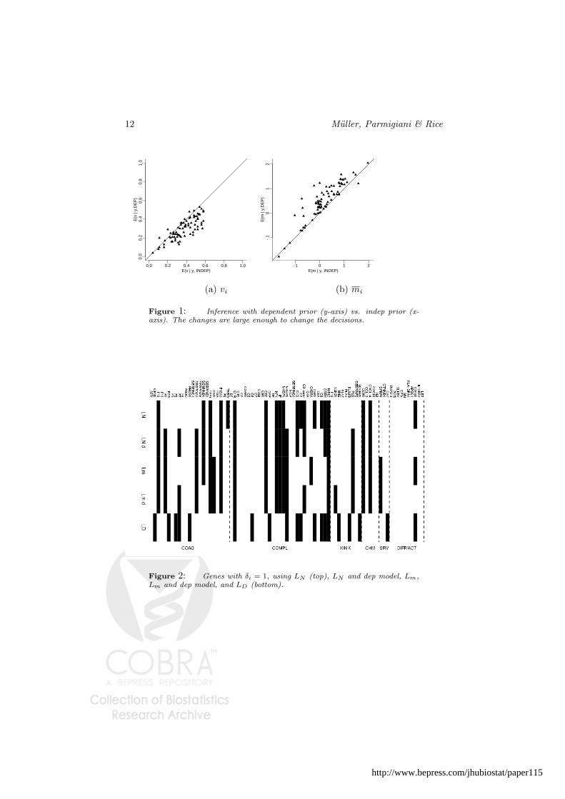
slightly when adjusting for dependence. The change in the estimates is shown inFigure 1. Although the changes are minimal for most genes, the impact in the finaldecision is visible. The first four rows of Figure 2 show the reported set of genesunder LN using the independent POE model (row 1) versus the dependent model(row 2), under Lm using the independent (row 3) and dependent (row 4) model.The last row shows inference under the loss function LD.

7. A PREDICTIVE LOSS FUNCTION

Microarray experiments are often carried out as hypothesis generating experiments,to screen for promising genes to be followed up in later experiments. Abruzzoet al. (2005) describe a setup, using RT-PCR to validate a list of differentiallyexpressed genes found in a microarray group comparison experiment. In particular,



0.0 0.2 0.4 0.6 0.8 1.0

0.0

0.2

0.4

0.6

0.8

1.0

E(v | y, INDEP)

E(v

| y,

DE

P)

−1 0 1 2−

10

12

E(m | y, INDEP)

E(m

| y,

DE

P)

(a) vi (b) mi

Figure 1: Inference with dependent prior (y-axis) vs. indep prior (x-axis). The changes are large enough to change the decisions.

Figure 2: Genes with δi = 1, using LN (top), LN and dep model, Lm,Lm and dep model, and LD (bottom).



they use TaqMan Low-Density Arrays for real-time RT-PCR (Applied Biosystems,Foster City, USA). They consider inference for nine samples from patients withchronic lymphocytic leukemia (CLL), using the microarray experiment for a firststep screening experiment, and the real-time RT-PCR to validate the identifiedgenes. With a setup like this experiment in mind we define a utility function that isbased on the success of a future followup study. To define the desired loss functionwe need to introduce some more detail of a joint probability model for the microarrayand real time RT-PCR experiments. Eventually we will use a stylized descriptionof inference in this model to define a loss function.

Let zit be a suitably normalized measurement for gene i in sample t, with ap-proximately unit marginal variance, var(zit) ≈ 1. For example, zit could be thelatent probit score in (7). Let yit denote the recorded outcome of the RT-PCR forgene i in sample t. The data are copy numbers, interpreted as base two logarithm ofthe relative abundance of RNA in the sample. Abruzzo et al. (2005) use a normallinear mixed effects model to calibrate the raw data against a calibrator sample andan endogenous control, chosen to reduce the variance of corrected responses acrosssamples. Let yit denote the calibrated pre-processed data. An important conclu-sion of the discussion in Abruzzo et al. (2005) is inference about the correlation ofthe microarray and RT-PCR measurements. They find a bimodal distribution ofcorrelations across genes. About half the genes show a cross-platform correlationρi ≈ 0.8, and half show essentially zero correlation, ρi = 0.

We introduce a simple hierarchical model to represent the critical features of thecross-platform dependence, and a realistic distribution of the RT-PCR outcomes.We build on the POE model described earlier, in (7) and (7), without necessarilyincluding the dependent model extension. Let zit denote the latent score in (7). Foryit we assume:

p(yit | zit, ρi) =

(zit with prob. ρi

N(0, 1) with prob. (1− ρi)(10)

with Pr(ρi = ρ?) = pρ and Pr(ρi = 0) = 1 − pρ. We use ρ? = 0.8 and pρ = 0.5 toapproximately match the reported inference in Abruzzo et al. (2005). Also, afterstandardization Abruzzo et al. (2005) found standard deviations in the RT-PCRoutcomes for each gene across samples in the range of approximately 0.5 through1.5 (with some outliers below and above). We chose the unit variance in the normalterm above to match the order of magnitude of these reported standard deviations.

Consider now the problem of reporting a list of differentially expressed genes ina microarray group comparison experiment. We assume that the selected genes willbe validated in a future followup real-time RT-PCR experiment, using, for example,the described TaqMan Low-Density Arrays. We build a loss function designed tohelp us to construct a rule that identifies genes that are most likely to achieve asignificant result in the followup experiment. For a stylized description we assumethat the followup experiment is successful for gene i if we can report a statisticallysignificant difference of expression across the two biologic conditions.

In words, the construction of the proposed loss function proceeds as follows.For each identified gene i we first select an alternative hypothesis. We then carryout a sample size argument based on achieving a desired power for this alternativeversus the null hypothesis of no differential expression, using a traditional notion ofpower. Next we find the posterior predictive probability of a statistically significantoutcome (Ri) for the future experiment. Finally, we define a loss function with



terms related to the posterior predictive probability for Ri and the sampling costfor the future experiment. The stylized description is not a perfect reflection ofthe actual experimental process. It is not even a reasonable model for actual dataanalysis. But we believe it captures the critical features related to the desireddecision of identifying differentially expressed genes. In particular, it includes anatural correction of statistical significance for the size of the effect.

Let xt ∈ {−0.5, 0.5} denote a (centered) indicator for the biologic condition ofsample t. Recall from (7) that the level of differential expression for gene i, mi, wasdefined as the probit regression coefficient for an indicator of the biologic condition.Let (mi, si) denote the posterior mean and standard deviation of mi. Let ρ = pρρ?

denote the assumed average cross-platform correlation, averaged across genes. Letµi1 = E(yit | xt > 0) and µi0 = E(yit | xt < 0) denote the mean expressionunder the two conditions in the followup experiment. For the upcoming sample sizeargument we assume a test of the null hypothesis H0 : µi1 − µi0 = 0 versus thealternative hypotheses H1 : µi1 − µi0 = m∗

yi, with m∗yi = ρ(mi − si), the mean

difference under an assumed alternative mi = mi − si. Let qα denote the (1 − α)quantile of a standard normal distribution. Assuming that upon conclusion of thefollowup experiment the investigators carry out a normal z-test, we find a requiredsample size

ni(z) ≥ 2ˆ(qα + qβ)/m∗

yi

˜2

for a given significance level α and power (1 − β). The sample size is a functionof the data z, implicitly through the choice of the alternative m∗

yi. Here samplesize refers to the number of samples under each biologic condition, i.e., the totalnumber of samples is 2n. Let yi0 and yi1 denote the sample average in the followup

experiment, for gene i and the two conditions. Let Ri = {(yi1 − yi0)p

n/2 ≥ qα}denote the event of a statistically significant difference for gene i in the followupexperiment. Let πi = Pr(Ri | Y ) denote the posterior predictive probability of Ri.Let Φ(·) denote the standard normal c.d.f.

πi(z) = (1− pρ)α + pρΦ

24ρ?mi1

pni/2− qαq

1 + n2ρ∗2s2

i

35 .

Combining ni and πi to trade off the competing goals of small sampling cost andhigh success probability we define a loss function

LF (δ, z) =Xδi=1

[−c1πi(z) + ni(z)] + c2D (11)

Under the loss function LF , the optimal rule is easily seen as

δ∗i = I(ni + c2 ≤ c1πi).

If we replace classical power by Bayesian power (Spiegelhalter et al., 2004, chapter6.5.3) then πi remains constant by definition, leaving only the bound on the samplesize ni. Also, c2 could be zero if the size of the reported short-list is not an issue.Figure 3 shows the optimal decision under LF for the EOC example (squares).We used c1 = 3000 and calibrated c2 such that the optimal decision reports D =20 genes, as before. The value for c1 was chosen to have the reward c1 matchapproximately 10 times the average sampling cost of a followup trial.



8. SUMMARY

Table 2 summarizes the proposed loss functions and rules. For all except LD the op-timal rule can be described as a threshold for an appropriate gene-specific summarystatistic of the data. Storey (2005) describes such rules as significance thresholding.The summaries are the marginal posterior probability of differential expression vi,posterior mean and standard deviation of the level of differential expression (mi, si),the sample size for a followup experiment ni, the posterior predictive probability of asignificant outcome πi, and the increment in posterior probability of non-differentialexpression ∆wB(i),i. The last three are functions of (vi, mi, si) only.

Table 2: Alternative loss functions and optimal rulesLoss function Rule

LN = cFD + FN δi = I(vi > t)

Lm = −∑

δimi + k∑

(1− δi)mi + cD δi = I(mi > t)

LD = −k1 log(|Σ1|)− k2

∑δifD(mi)+

+k3

∑(1− δi)fN (mi) + k4D no closed form

LF =∑

δi=1(−c1πi + ni) + c2D δi = I(ni + c2 ≤ c1πi)

LU = FDR/α− g(D) δi = I(vi ≥ vj) withj = maxi

{i : ∆wi,B(i) ≤ α i/n

}In summary, all optimal rules are computed on the basis of only a few under-

lying summaries. This makes it possible to easily consider multiple rules in a dataanalysis. Critical comparison of the resulting rules leads to a finally reported set ofcomparisons. In some cases the application leads to a different loss function. Goodexamples are the loss functions considered in Lin et al. (2004). If a specific lossfunction arises from a specific case study, it should be used.

The loss function LD requires the additional summary Σ1(δ). Let S denote acovariance matrix of the relevant latent variables for all genes that are considered forreporting in LD. The desired Σ1(δ) for any subset of selected genes is then computedas the marginal correlation matrix for that subset. Let Sδ denote the submatrixdefined by choosing rows and columns selected by δ. Let λi = 1/

√Sii, and λδ denote

the vector of λi corresponding to the reported genes. We use Σ1(δ) = λδ[Sδ]λ′δ. This

reduces δD to a function of m and S only.Figure 3 compares the reported gene lists for the loss functions LN , Lm and

LD, under the independent model and the dependent model. For many genes thedecision remains unchanged across all loss functions. For some genes with highprobability of differential expression, but small level of differential expression, andvice versa, the decision depends on whether or not the terms in the loss functionare weighted by mi.

9. DISCUSSION

We have reviewed alternative approaches to addressing problems related to massivemultiple comparisons. Starting from traditional rules that control expected FDR,with the expectation over repeated sampling, we have discussed the limitation of the



RA

NK

SIG

N T

HR

ES

H.

●● ●

●● ●

●●

●

●

●

●

●

●

● ● ●

●

●

●

●

●

●

●

●

●

●

● ●

● ●

●

●

●

●●

●

●●

●● ●

●

●

●

● ●

●

●

●

●

●

●

●

●●

●

●

●

●

● ●

●

● ●

●

●

●

●

● ●

● ●

●

●

●

●●

●

●● ●

●●

●

●

● ● ●

● ●

●●

●

●

●

●

●

●

●

● ●

●

●

● ●

● ●●

●

●

●

●●

●

●

●

●

● ● ●

●

●

●

● ●

●

● ●

●

●

●

●

●

●

●

●

●

●

●

●

●

●

● ●

●

●

●●

●

●

●●

●

●

●

●

●

TF

PI

CC

R1

F13

A1

F10

CR

2C

XC

L14

IF CD

163

HF

1M

BL2

MA

SP

2C

1RP

LGS

ER

PIN

D1

VW

FS

FR

P4

SE

RP

INA

1F

2RM

AS

P1

DF

F7

C4B

PA

F2

PLA

U

F9

CR

RY

TH

BD

C5R

1C

9

C3

C3−

conv

C1Q

●

●

v INDEPv DEPm INDEPm DEPPRED

Figure 3: Comparison of optimal rules for LN (circles) under theindependent model (black) and dependent model (light gray), Lm (triangle)under the independent (black) and dependent model (gray), and LF (square).For each gene (horizontal axis) symbols are plotted against the rank of thecorresponding significance threshold statistic (vertical axis). The reportedgenes under each rule are the top 20 ranked genes (above the dashed horizontalline). The symbols corresponding to selected genes are filled. The names ofselected genes are shown on the vertical axis. Genes are sorted by averagerank under the five criteria.

interpretation of these decisions as Bayesian rules. We have argued for a solutionof the massive multiple comparisons as a decision problem, and we have shown howthis is implemented in structured probability models including dependence acrossgenes. Most, but not all, loss functions lead to rules that can be defined in terms ofa significance thresholding function, S(data), as proposed in Storey (2005).

The proposed approaches are all based on casting the multiple comparison prob-lem as a decision problem and thus inherit the limitations of any decision theoreticsolution. In particular, we recognize that not all research is carried out to makea decision. The decision theoretic perspective might be inappropriate when an ex-periment is carried out for more heuristic learning, without being driven by specificdecisions. Also, all arguments were strictly model-based. Even results that apply forany probability model still need a specific probability model to implement relatedapproaches. Like any model-based inference, the implementation involves the oftendifficult tasks of prior elicitation, and the choice of appropriate parametric models.Additionally, our arguments require the choice of a utility function. A commonfeature of early stage hypothesis generating experiments is that they serve multipleneeds. We might want to carry out a microarray experiment to suggest interestinggenes and proteins for further investigation, to propose suitable candidates for acorrelation study with clinical outcomes, and also to simply understand molecularmechanisms.

We caution against over-interpretation of results based on highly structuredprobability models and often arbitrary choices of utility functions. Data analysis for



high-throughput gene expression data is particularly prone to problems arising fromdata pre-processing. Often it is more important to understand the pre-processingof the raw data, and correct it if necessary, than to spend effort on sophisticatedmodeling. Specifically related to the dependent probability model, it is importantto acknowledge limitation of pathway information that is used to select the set ofpossible parent nodes Ni in (8) when constructing the dependent probability model.Pathway information does not necessarily describe relations among transcript levels,although it carries some information about it.

We have focused on the inference problem of reporting lists of differentiallyexpressed genes, and inference on massive multiple comparisons in general. A similarframework, using the same probability models and loss functions, can be used forother decision problems related to the same experiments. For example, one couldconsider choosing the sample size for a future experiment (sample size selection),ranking genes or selecting a fixed set of genes (for a panel of biomarkers).

Acknowledgments

Research was supported by NIH/NCI grant 1 R01 CA075981 and by NSF DMS034211.Kenneth Rice was supported by Career Development Funding from the Departmentof Biostatistics, University of Washington

REFERENCES

Baggerly, K. A., Morris, J. S., Wang, J., Gold, D., Xiao, L. C. and Coombes, K. R. (2003)A comprehensive approach to analysis of MALDI-TOF proteomics spectra from serumsamples. Proteomics, 9, 1667–1672.

Bayarri, M. J. and Berger, J. O. (2000) P values for composite null models. J. Amer.Statist. Assoc. 95, 1127–1142.

Benjamini, Y. and Hochberg, Y. (1995) Controlling the false discovery rate: A practicaland powerful approach to multiple testing. J. Roy. Statist. Soc. B 57, 289–300.

Berry, D. A. and Hochberg, Y. (1999) Bayesian perspectives on multiple comparisons.J. Statist. Planning and Inference 82, 215–227.

Berry, S. and Berry, D. (2004) Accounting for multiplicities in assessing drug safety: Athree-level hierarchical mixture model. Biometrics 60, 418–426.

Casella, G. and Berger, R. L. (1987) Reconciling Bayesian and frequentist evidence in theone-sided testing problem. J. Amer. Statist. Assoc. 82, 106–111.

Cohen, A. and Sackrowitz, H. B. (2005) Decision theory results for one-sided multiplecomparison procedures. Ann. Statist. 33, 126–144.

— (2006) More on the inadmissibility of step-up. Tech. rep., Rutgers University.

Do, K., Muller, P. and Tang, F. (2005) A bayesian mixture model for differential geneexpression. Appl. Statist. 54, 627–644.

Duncan, D.B. (1965) A Bayesian Approach to Multiple Comparisons, Technometrics 7,171-222.

Efron, B. and Tibshirani, R. (2002) Empirical bayes methods and false discovery rates formicroarrays. Genetic Epidemiology, 23, 70–86.

Efron, B., Tibshirani, R., Storey, J. D. and Tusher, V. (2001) Empirical Bayes analysis ofa microarray experiment. J. Amer. Statist. Assoc. 96, 1151–1160.

Fortini, M., Liseo, B., Nuccitelli, A. and Scanu, M. (2001) On bayesian record linkage.Research in Official Statistics, 4, 185–198.

— (2002) Modelling issues in record linkage: a bayesian perspective. In Proceedings of theASA meeting. ASA, ASA.

Genovese, C., Lazar, N. and Nichols, T. (2002) Thresholding of statistical maps inneuroimaging using the false discovery rate. NeuroImage, 15, 870–878.



Genovese, C. and Wasserman, L. (2002) Operating characteristics and extensions of thefalse discovery rate procedure. J. Roy. Statist. Soc. B 64, 499–518.

— (2003) Bayesian and Frequentist Multiple Testing. Bayesian Statistics 7 (J. M.Bernardo, M. J. Bayarri, J. O. Berger, A. P. Dawid, D. Heckerman, A. F. M. Smithand M. West, eds.) Oxford: University Press, pp. 145-162.

Gopalan, R. and Berry, D. A. (1998) Bayesian multiple comparisons using Dirichletprocess priors. J. Amer. Statist. Assoc. 93, 1130–1139.

Keeney, R. L., Raiffa, H. A. and Meyer, R. F. C. (1976) Decisions With MultipleObjectives: Preferences and Value Tradeoffs. New York: Wiley

Lin, R., Louis, T. A., Paddock, S. M. and Ridgeway, G. (2004) Loss function basedranking in two-stage hierarchical models. Tech. rep., Johns Hopkins University, Dept.of Biostatistics.

Lindley, D. V. (1971) Making decisions. New York: WileyMuller, P. and Parmigiani, G. (2006) Modeling dependent gene expression. Tech. rep.,

M.D. Anderson Cancer Center.Muller, P., Parmigiani, G., Robert, C. and Rouseau, J. (2004) Optimal sample size for

multiple testing: the case of gene expression microarrays. J. Amer. Statist. Assoc. 99,990-1001.

Newton, M., Noueriry, A., Sarkar, D. and Ahlquist, P. (2004) Detecting differential geneexpression with a semiparametric heirarchical mixture model. Biostatistics, 5, 155–176.

Newton, M. A., Kendziorsky, C. M., Richmond, C. S., R., B. F. and Tsui, K. W. (2001)On differential variability of expression ratios: improving statistical inference aboutgene expression changes from microarray data. Journal Computational Biology, 8,37–52.

Parmigiani, G., Garrett, E. S., Anbazhagan, R. and Gabrielson, E. (2002) A statisticalframework for expression-based molecular classification in cancer. J. Roy. Statist.Soc. B 64, 717–736.

Ronning, G. and Kukuk, M. (1996) Efficient estimation of ordered probit models.J. Amer. Statist. Assoc. 91, 1120–1129.

Scott, J. and Berger, J. (2003) An exploration of aspects of bayesian multiple testing.Tech. rep., Duke University, ISDS.

Sellke, T., Bayarri, M. J. and Berger, J. O. (2001) Calibration of p values for testingprecise null hypotheses. Amer. Statist. 55, 62–71.

Shen, W. and Louis, T. A. (1998) Triple-goal estimates in two-stage hierarchical models.J. Roy. Statist. Soc. B 60, 455–471.

Shen, X., Huang, H.-C. and Cressie, N. (2002) Nonparametric hypothesis testing for aspatial signal. J. Amer. Statist. Assoc. 97, 1122–1140.

Storey, J. (2002) A direct approach to false discovery rates. J. Roy. Statist. Soc. B 64,479–498.

— (2005) The optimal discovery procedure I: a new approach to simultaneous signficancetesting. Tech. Rep. 259, University of Washington.

Storey, J. D. (2003) The positive false discovery rate: A Bayesian interpretation and theq-value. Ann. Statist. 31, 2013–2035.

Storey, J. D., Taylor, J. E. and Siegmund, D. (2004) Strong control, conservative pointestimation and simultaneous conservative consistency of false discovery rates: a unifiedapproach. J. Roy. Statist. Soc. B 66, 187–205.


Date post:	25-Mar-2018
Category:	Documents
Upload:	lamkiet
View:	217 times
Download:	1 times

FDR and Bayesian Multiple Comparisons Rulesbrad/7440/MuellerParmigianiRice… · · 2008-12-22FDR...

Documents