34
FE modelling of Wood Structure Petr Koňas 3.června 2008, Dolní Maxov Ing. Petr Koňas, Ph.D.
| Date post: | 11-Dec-2015 |
| Category: |
Documents |
| Upload: | cole-meese |
| View: | 214 times |
| Download: | 0 times |

FE modelling of Wood StructurePetr Koňas
3.června 2008, Dolní MaxovIng. Petr Koňas, Ph.D.
Programy a algoritmy numerické matematiky 14
strana 2/33
Guidelines• Why to model wood structure?• Problems of geometry
– Disadvantages of homogenized models.– Problems in modelling of biol.structures.– Problem of anisotropy.– How deep? Low limits in modelling.– Problem of variability.– Probable structure – probable results.– Accuracy– How far? Up limits in modelling.– What a time?– Advantages and disadvantages of L-systems
• Coupled physical task • Weak solution with mixed multiscaled finite elements

Programy a algoritmy numerické matematiky 14
strana 3/33
Why model wood structure?
- Homogenized models fails- Common models may be too complicated for accurate solution- Although the physical model exists on lower scale, it can be difficult to find
appropriate solution on higher scale(s)- Microscopic and lower scaled structures became more important than before mainly for nanotechnology and material science- Evaluation of material model “ab initio” may be more efficient than expensive experiments- Wood and several other parts are structures with remodelling character and
its development in time (growing) is closely connected to micro and meso-scales.
- Modelling on lower scales can help us to understand more the substance and reasons of final behaviour of wood.

Programy a algoritmy numerické matematiky 14
strana 4/33
Disadvantages of homogenized models- Reduce information with local character, even though it can influence higher
scales- Wood is anisotropic material with high variability. It is difficult to determine
appropriated reference region.- Material properties embody variability according to scales. Accuracy of solution
on some scale level can be very poor in extension on lower or higher scales. Also accuracy on the same scale can be far off constant character.
- When some reference region is chosen, the problem of material properties is still not solved.

Programy a algoritmy numerické matematiky 14
strana 5/33
• Generally insufficient amount of input parameters and verifying experiments.• How can we simply describe geometry of biol. structures? • How to describe variability of material properties (according to structure, scale, environment)?• How to describe relationship of material and geometry properties on scale? • How to determine influence of properties from specific scale on behaviour on higher scales? (vegetation × abiotic factors, stand × fluid flow, tree × bush, crown/roots × stem, heartwood × sap, early × late wood, tracheids × parenchyma cells, lumen × cell layers, lignin × cellulose, covalent × ion coupling, quantum effects)
• How to involve “individuality” and “stereotype”? (selfsimilar/fractal structure × individual occurrence/mutation)• How to involve genetic predetermination and phenotypic resignation?
Problems in modelling of biol.structures
Programy a algoritmy numerické matematiky 14
strana 6/33
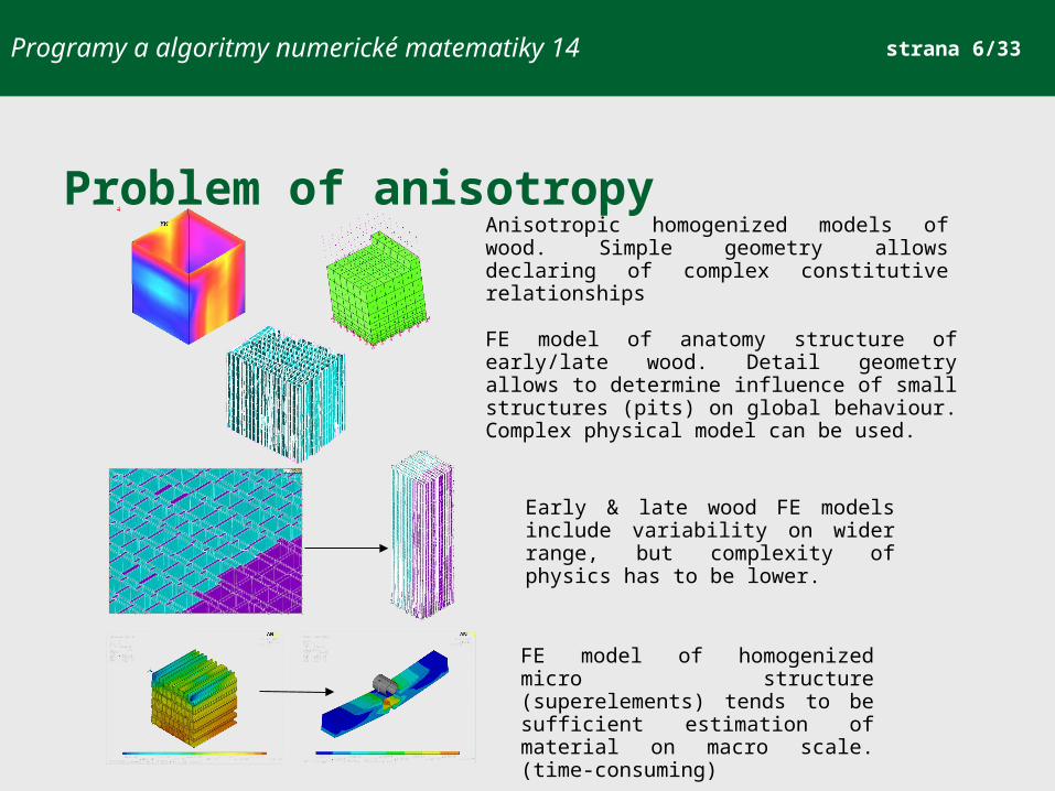
Problem of anisotropyAnisotropic homogenized models of wood. Simple geometry allows declaring of complex constitutive relationships
FE model of anatomy structure of early/late wood. Detail geometry allows to determine influence of small structures (pits) on global behaviour. Complex physical model can be used.
Early & late wood FE models include variability on wider range, but complexity of physics has to be lower.
FE model of homogenized micro structure (superelements) tends to be sufficient estimation of material on macro scale. (time-consuming)

Programy a algoritmy numerické matematiky 14
strana 7/33
How deep?
Early and late type of tracheid
Early and late wood transition
Cell wall with layered elements
Orientation of fibrils in individual layers

Programy a algoritmy numerické matematiky 14
strana 8/33
Problem of variabilityProbabilistic structure
How to determine structure of wood for arbitrary position?If statistical behaviour of morphological parameters can be determined, the cross-scale relationships (transition functions) can be evaluated.

Programy a algoritmy numerické matematiky 14
strana 9/33
Near the stem pith Far off the stem pith
Shear RL Shear RT Shear TL
etc.
Probable structure – probable results
Tensionx
Compression

Programy a algoritmy numerické matematiky 14
strana 10/33
Accuracy?
Accuracy and large amount of material characteristics provide “accurate” results on statistical sense. “Accuracy” can be also in 30% of variation coefficient. This problem origins from assumption, that geometry has stochastic character (this assumption coincides with the similar statement that material properties has stochastic character), but geometry is consequence of developing stage (growing) and material in every position in stem is not independent, but it is related to position, environment, conditions, etc.Probabilistic FE model are unsuitable for homogenization and solution on higher scales.
Solution of such problem can be evolutionary models.

Programy a algoritmy numerické matematiky 14
strana 11/33
How far?
A=aaSaaSaaSaaSaaSaaSaaSaaSaaSaaBS='(.9)!(.9)a=tF[&'(.8)!B|z]>(137)[z&'(.7)!B|z]>(137)B=tF[-'(.8)!(.9)$C|z]'(.9)!(.9)CC=tF[+'(.8)!(.9)$B|z]'(.9)!(.9)B
A=F[&'(.7)!B]>(137)[&'(.6)!B]>(137)'(.9)!(.9)AB=F[-'(.7)!(.9)$C]'(.9)!(.9)CC=F[+'(.7)!(.9)$B]'(.9)!(.9)B
c(12)FFFFFFFFFF>(1)&(1)AA=!(.75)t(.9)FB>(94)B>(132)BB=[&"t(.9)!(.75)F[|z]$A[|z]]
c(12)AA=aaSaaSAS='(.8)!(.9)a=tF[&'(.8)!B]>(137)[z&'(.7)!B]>(137)B=tF[-'(.8)!(.9)$C]'!(.9)CC=tF[+'(.8)!(.9)$B]'!(.9)B
c(12)FFFFFAA=!(.8)tFB>(94)C>(132)DB=[&'t(.5)!(.9)F$A|z]C=[&'t(.4)!(.8)F$A|z]D=[&'t(.3)!(.7)F$A|z]
Orthotropic material properties, gravitational acceleration, non axis force, base of stem is fixed, 840-1500 geometric components, 100 000-1 200 000 finite elements, 5 mil.DOFs.
Lindenmayer grammar allows to create iterated structures with selfsimilar/fractal character as on micro scale as on macro scale. With FE translator very complex geoms can be numerically solved.

Programy a algoritmy numerické matematiky 14
strana 12/33
What a time?
A =
!(.
8)tF
B>
(94)
C>
(132
)DB
= [
&'t(
.5)!
(.9)
F$A
L|z
L]
C =
[&
't(.4
)!(.
8)F$
AL
|zL
]D
= [
&'t(
.3)!
(.7)
F$A
L|z
L]
L =
[~c
(8){
+(3
0)f(
.5)-
(120
)f(.
5)-(
120)
f(.5
)}]
A =
aaSaaS
aaSaaS
aaSaaS
aaSaaS
aaSaaB
S =
'(.9)!(.9)a =
tF[&
'(.8)!LB
L|zL
]>(137)[z&
'(.7)!LB
L|zL
]>(137)
B =
tFL
[-'(.8)!(.9)$LC
L|zL
]'(.9)!(.9)CC
= tF
L[+
'(.8)!(.9)$LB
L|zL
]'(.9)!(.9)B
L =
[~c(8){+(30)f(.4)-(120)f(.4)-(120)f(.4)}]
L-systems
Also evolutionary models can be analyzed by Lindenmayer systems

Programy a algoritmy numerické matematiky 14
strana 13/33
Advantages and disadvantages of L-systems
Advantages- L-systems seems to be very realistic (according to geometry and description of material
properties distribution)- Models derived by iterated functions include less unknowns and offers tool for evaluation
of variables which depends on geometry (permeability, variation of properties)- Model assembling can be less data-intensive - Predictive abilities can be higher in comparison with homogenized models
Disadvantages- L-system based models translated finite element mesh are still very huge- Formed models are usually very complicated- Iterated function for geometry of structure has to be revealed.- Solution is very difficult for coupled physical problems- It is multispecialty, money and time consuming problem
Programy a algoritmy numerické matematiky 14
strana 14/33
Coupled physical task
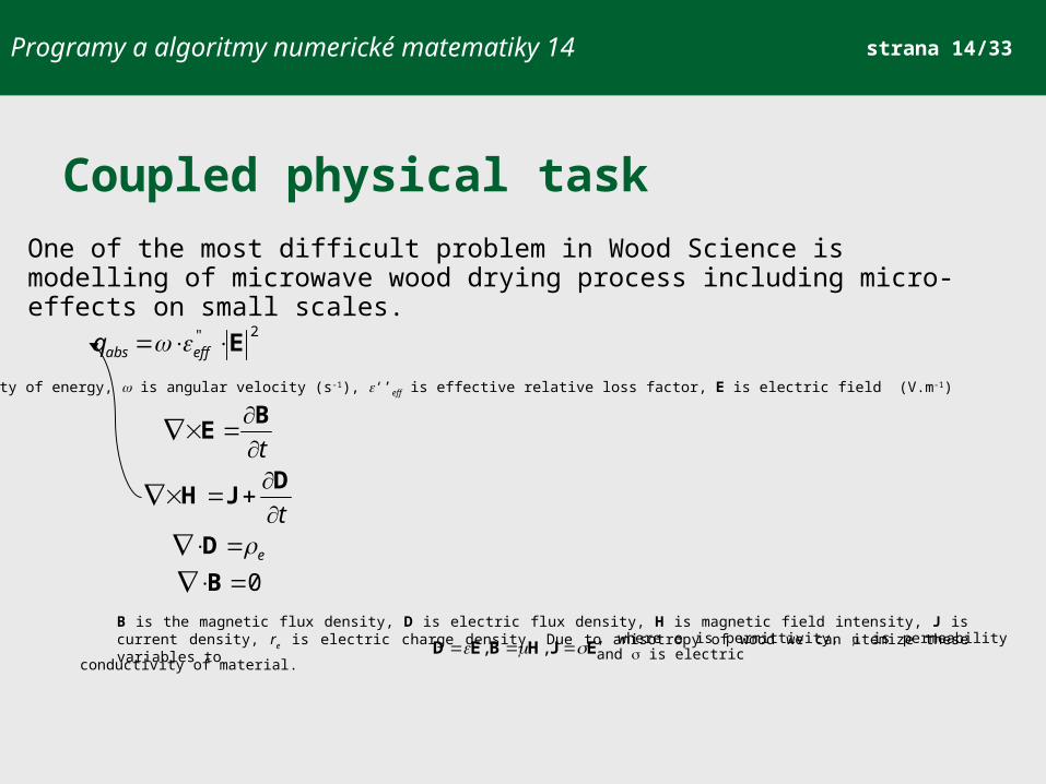
One of the most difficult problem in Wood Science is modelling of microwave wood drying process including micro-effects on small scales.
2'' E effabsq
qabs is density of energy, is angular velocity (s-1), ‘’eff is effective relative loss factor, E is electric field (V.m-1)
0
B
D
DJH
BE
e
t
t
B is the magnetic flux density, D is electric flux density, H is magnetic field intensity, J is current density, re is electric charge density. Due to anisotropy of wood we can itemize these variables to EJHBED , , , where e is permittivity, is permeability and is electricconductivity of material.

Programy a algoritmy numerické matematiky 14
strana 15/33
Coupled physical taskWhen only conduction due to the microwave heating source is considered:
absqTt
TC
k
When also convective source plays important role:
TTkqTtT
C exthabs T
k
Temperature is not only one of important fields, which is changing during drying process
ppTpwt
p
wwTpwt
w
TTqTpwt
TC
ext
ext
extabs
p
w
T
hpTpppw
hwTwpww
hTTTpTw
kkkk
kkkk
kkkk

Programy a algoritmy numerické matematiky 14
strana 16/33
Coupled physical taskRapid change of moisture, temperature are reasons for large time-depended stress-strain effect.
t
t
vel
celc
εDε
σ
elc is immediate elastic strain (structural), vel
c is viscous-elastic part of strain (structural), F() is function of memory effect, D is matrix of
elasticity, is relaxation time
Both strains are composed from pure mechanical, thermal and moisture components
velT
velw
velvelc
elT
elw
elelc
εεεε
εεεε
In our case the problem was simplified for visco-elastic strains
velTw,
velc εε
or for constant memory effectt
elc
velTw,
Tw,
ελDεσ

Programy a algoritmy numerické matematiky 14
strana 17/33
Coupled physical task
Elastic components has usual linear character
βε
αε
elT
elw
extext
elw
elwel
welw
elw
TTTT
HLwk
HLkk
HLw
kHLw
k
654321
654321
|||||
for 0
for w 1,1|||||1
Also elastic mechanical properties for pure mechanical behaviour should include linear influence of moisture and temperature
extbextbrw
extbextbrw
TTkwwkGG
TTkwwkEE
Tj
wjjj
Ti
wiii
HLwk
HLwkk
wi
wi
wi
b
b
b for 0
for 0
Programy a algoritmy numerické matematiky 14
strana 18/33
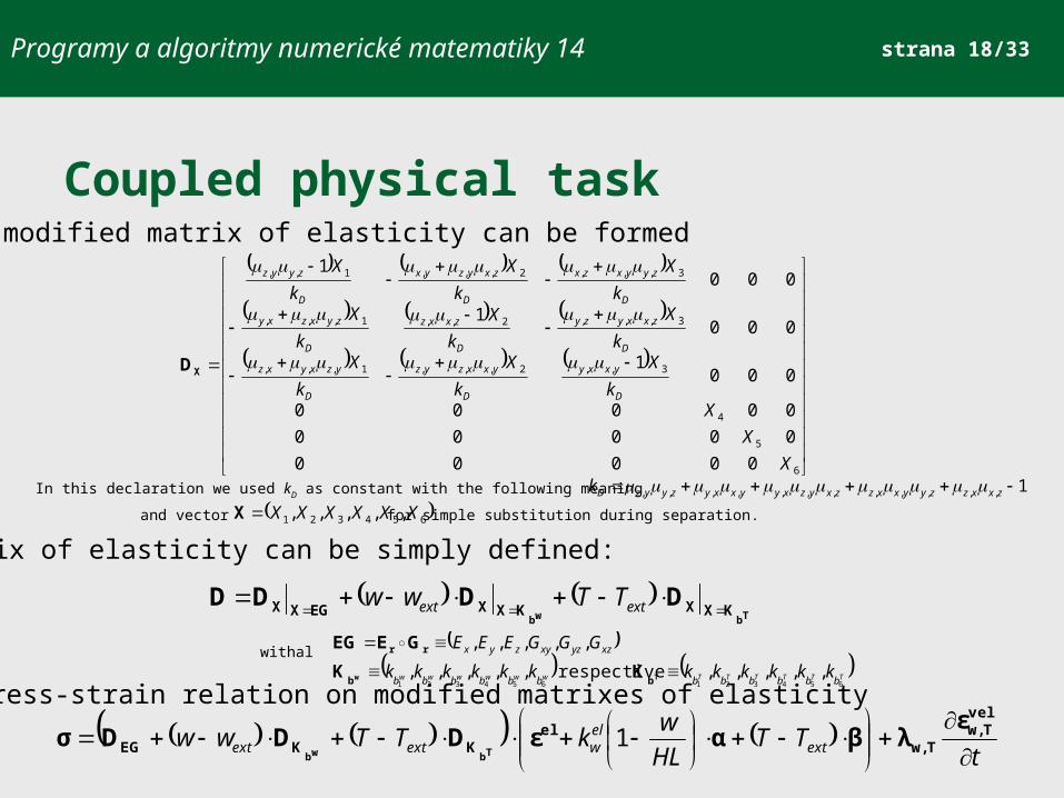
Coupled physical taskThan modified matrix of elasticity can be formed
6
5
4
3,,2,,,1,,,
3,,,2,,1,,,
3,,,2,,,1,,
00000
00000
00000
0001
0001
0001
X
X
Xk
X
k
X
k
Xk
X
k
X
k
Xk
X
k
X
k
X
D
yxxy
D
yxxzyz
D
yzxyxz
D
zxxyzy
D
zxxz
D
zyxzxy
D
zyyxzx
D
zxyzyx
D
zyyz
XD
1,,,,,,,,,,,, zxxzzyyxxzzxyzxyyxxyzyyzDk 654321 ,,,,, XXXXXXX
In this declaration we used kD as constant with the following meaning
and vector for simple substitution during separation.
Matrix of elasticity can be simply defined:
Tbwb
KXXKXXEGXX DDDD
extext TTww
withal
TTTTTTwwwwww bbbbbbbbbbbb
xzyzxyzyx
kkkkkkkkkkkk
GGGEEE
654321654321,,,,, respective ,,,,,
,,,,,
Tw bb
rr
KK
GEEG
Final stress-strain relation on modified matrixes of elasticity
t
TTHL
wkTTww ext
elwextext
velTw,
Tw,el
KKEG
ελβαεDDDσ
Tbwb
1

Programy a algoritmy numerické matematiky 14
strana 19/33
Coupled physical taskPrevious equation has to be disassembled into unknown displacement by the common relationships.
ij
ij Fxt
2
2u
velvelvelvel wvu
z
u
x
w
y
w
z
v
x
v
y
u
z
w
y
v
x
u
z
u
x
w
y
w
z
v
x
v
y
u
z
w
y
v
x
u
,,
2
1
2
1
2
1
2
1
2
1
2
1
111111111
u
ε
ε
velTw,
el
u is vector of displacements wvu ,,u , Fi are components of volume forces

Programy a algoritmy numerické matematiky 14
strana 20/33
The final relationship for stress-strain components according to unknown variable displacement u respective uvel can be formed in this grouped form.
FCCCCCC
ucuccc
u
wTTTww
velλKKEG
22
Tw,Tbwb
wTTTww
tTTww
t extext
22
2
2
βαDDDCαDβDC
βDCβαDβDDC
αDCβαDαDDC
TbwbTbwb
Tb2
Tbwb
wb2
wbTb
KKEGKKwT
KTKKEGT
KwKKEGw
extelwextext
elw
extelwext
elw
extextel
wext
elw
TkTwHL
k
Tkw
HL
kT
HL
wkT
HL
k
;
;2
;1
333231
5521
5521
6621
6621
5521
5521
232221
4421
4421
6621
6621
4421
4421
131211
000000
0000000
0000000
0000000
000000
0000000
0000000
0000000
000000
XXX
XX
XX
XX
XXX
XX
XX
XX
XXX
DDD
DD
DD
DD
DDD
DD
DD
DD
DDD
Xc
TTbbwb
wb KXXKKXXKEGXXEG cccccc
,,
3541
641
521
541
621
641
541
521
541
2441
421
441
641
621
441
421
641
441
1
000000
0000000
0000000
0000000
000000
0000000
0000000
0000000
000000
Tw,c

Programy a algoritmy numerické matematiky 14
strana 21/33
Coupled physical task
ppTpwt
p
wwTpwt
w
TTqTpwt
TC
ext
ext
extabs
p
w
T
hpTpppw
hwTwpww
hTTTpTw
kkkk
kkkk
kkkk
2'' E effabsq
Described model is valid for diffusive transport of moisture and temperature. It is not appropriate (due physical nature of phenomenon) for free water movement. This transport is allocated into intercellular spaces and cell lumen. Description of this process can be done with Navier-Stokes equation. Finally the following set of PDE’s has to be solve:
flptzyx
ν
νF
ν 22
2
1
FCCCCCC
ucuccc
u
wTTTww
velλKKEG
22
Tw,Tbwb
wTTTww
tTTww
t extext
22
2
2

Programy a algoritmy numerické matematiky 14
strana 22/33
0,2
,,,
22
2
2
ξCCCCCCF
ξu
cξucccξu
wTTTww
velλKKEG
22
Tw,Tbwb
wTTTww
tTTww
tF extextu
The weak form of thermal-moisture displacements can be written as follows:
0H , for all and meaning of as scalar product on Hilbert space.
1
11m
VVVV m 1
1
11 ,,, 21 ijV j
j 1for
VVVVVV m 11
1
111 ,,321
Let us assume the region is partitioned by linear mesh on very fine scale also we will assume that region is not of small regions are covered by mesh on this scale (subgrids).
, where are Raviart-Thomas (RT) spaces.
fully partitioned by this fine mesh. Only
Functional is than defined on vector subspaces Subspaces may not fill the full space V. It means that
1
1
1
11
1
1
1
1
11
22
1
2
1
2
11
11
1
1
1
1 ,2,1,2,2,1,1,2,1, ,,,,,,,, mnVVVnVVVnVVV VVVmmmm
11
11
1
1
1
1
1
22
1
2
1
2
1
11
1
1
1
1
1,2,1,,2,1,,2,1, ,,,,,,, V
mmmm nVVVnVVVnVVV 1V
Withal we declare mentioned vector subspaces with bases
Complete basis on vector space
i ,,,
32
i 21 immm ,,, 32
VVVVVVVVVVVV iiimmm
2
3
2
332
2
22 ,,,,,,,,,,,, 212121
Similarly let us to partition by next linear meshes for different scales where again
regions cover some parts of on specific scale. Consequently similar vector subspaces can be distinguished
with the same requirements:
.,,
,
,,,
,,,
2
23
2
33
12
2
22
21
21
21
VVVVV
VVVVV
VVVVV
iiiim
m
m
Weak solution

Programy a algoritmy numerické matematiky 14
strana 23/33
1
1 from 1 V
1
1 from 2 V
2
2 from 1 V 2
2 from 2 V
3
3 from 1 V

Programy a algoritmy numerické matematiky 14
strana 24/33
Weak solution
VfA uu :
uf,uu, 2 AuF
All unknowns can be decomposed to individual scales e.g.: oi someon 21 uuuu
Decomposition of unknowns to individual scales affects solution in sense of finite elements and minimisation of functional (1) does not provide common appearance of Ritz system
Let us consider PDE with differential operator A and follow common steps in solution of this task for multi-scale problem.
Functional which will be minimized has standard form:
Decomposed unknown will be substituted into first part of functional: AuiiL uuuuuu 2121 ,
A
AA
AAA
u
ii
i
i
uu
uuuu
uuuuuu
L
,
,2,
,2,2,222
12111
ji
jjj
s
kkkb
1
~ u
1
j
jjj
s
kkka
1
u
It can be expanded due to rules of scalar product in the following manner.
As usual the functional is minimized by the function:
For first step we will approximate functional in subgrid on scale
Finally unknown function can be by this function:
Programy a algoritmy numerické matematiky 14
strana 25/33
ju ~
k
k
j
j
k
k
j
j
k
k
jk
k
jkjkj
k
k
jk
k
jkjkjkjkj
kj
ssss
ss
ss
bb
bbbb
bbbbbb
uu
,
,2,2
,2,2,
~,~222222
1121211111
kj for
2
22
2
222
112121
2
111
,
,2,2
,2,2,
~,~
j
j
j
j
j
j
j
j
jj
j
jjjj
j
j
jj
j
jjjjjjjj
jj
sss
ss
ss
b
bbb
bbbbb
uu
iis
iis
iiss
i
iiis
iis
iiss ababababs
u
abababab
u
b
L
b
L
11
11
11
11
1111
11
11
11
11
1
,,,,1
,,
kj
a
a
a
buu
buu
buu
j
j
j
j
k
k
j
j
k
k
jk
k
j
kjkj
kj
k
k
kj
k
kj
k
kj
sAssAsAs
AA
A
s
for
,,2,2
0,,2
00,
~,~
~,~
~,~
2
1
21
2221
11
2
1
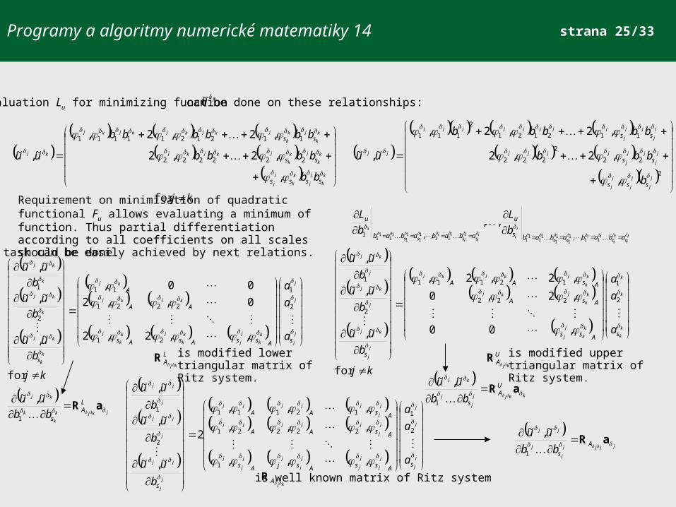
Evaluation Lu for minimizing function can be done on these relationships:
Requirement on minimisation of quadratic functional Fu allows evaluating a minimum of function. Thus partial differentiation according to all coefficients on all scales should be done.This task can be easily achieved by next relations.
jkjk
k
k
kjLA
sbbuu
aR
1
~,~
LA
kjR is modified lower triangular
matrix of Ritz system.
kj
a
a
a
b
uu
b
uu
b
uu
k
k
k
k
k
k
j
j
k
k
jkj
k
k
jkjkj
j
j
kj
j
kj
j
kj
sAss
AsA
AsAA
s
for
,00
,2,0
,2,2,
~,~
~,~
~,~
2
1
222
12111
2
1
kkjj
j
j
kjUA
sbb
uu
aR
1
~,~
UA
kjR is modified upper triangular
matrix of Ritz system.
j
j
j
j
j
j
j
j
j
j
jj
j
j
j
j
jjjjj
j
j
jjjjj
j
j
jj
j
jj
j
jj
sAssAsjAs
AsAA
AsAA
s
a
a
a
b
uu
b
uu
b
uu
2
1
1
22221
12111
2
1
,,,
,,,
,,,
2
~,~
~,~
~,~
jjjj
j
j
jj
A
sbb
uu
aR
1
~,~
kjA
R is well known matrix of Ritz system

Programy a algoritmy numerické matematiky 14
strana 26/33
Weak solutionApplying of mentioned rules on left part of functional leads to:
iii
i
i
ii
ii
ii
ii
A
LA
LA
s
u
UA
UAA
LA
LA
s
u
UA
UAA
LA
s
u
UA
UAA
s
u
bb
L
bb
L
bbL
bb
L
aR
aR
aR
aRaRaR
aR
aR
aRaRaR
aR
aRaRaR
2
2
22
2
2
22
2
22
22
11
2
3443333
232
131
3
2
3
2332222
121
2
2
2
12211111
1
1
1
1
1
1
This complex system can be rewritten in more readable form:
1
112
1
22j
k
LA
i
jk
UAA
s
u
u
u
A kjkkkjjjj
j
j
j
j
b
L
b
Lb
L
S
aRaRaR

Programy a algoritmy numerické matematiky 14
strana 27/33
j
j
j
j
kjkkkjjjj
j
j
j
j
s
j
k
LA
i
jk
UAA
s
u
u
u
A
f
f
f
b
L
b
Lb
L
S
,
,
,
22 2
1
1
112
1
aRaRaR
0,,0
1111
11
11
1111
11
11
11
11
1
,,,,1
iis
iis
iiss
i
iiis
iis
iiss ababababs
u
abababab
u
b
F
b
F
ja
j
j
j
j
sc
c
c
CBA
f
f
f
SSS
,
,
,
2 2
1
When the full functional is minimized by:
The solution of the initial problem can be reached by enumeration of
By analogy, the solution of coupled problem with applying of SA derivation can be rewritten.
for differential operator
0,2
,,,
22
2
2
ξCCCCCCF
ξu
cξucccξu
wTTTww
velλKKEG
22
Tw,Tbwb
wTTTww
tTTww
tF extextu
tC
TTwwBt
A extext
Tw,
Tbwb
λ
KKEG
c
ccc ,,2
2
CCCCCCF wTTTww 22 wTTTwwf c22
For differential operators
and function

Programy a algoritmy numerické matematiky 14
strana 28/33
Weak solutionSolution is realized in i consequent steps of solution. In first step the previous equation is formed, whereas results of higher scales are unknown (in Ritz or modified Ritz system). Solution on higher scales in individual nodes can be expressed by mapping of
1a
From this step we obtain definitions in some nodes on higher scale(s) which bounds region of element on this solved scale. In the following we calculate the same eq., but on the following higher scale withal some nodes on this scale were strictly derived from previous step. This idea is repeated until the highest scale is reached. Advantage of this type of solution is also that you do not need enumerate results on lower scales, but you can enumerate only results on last scale whereas results on this scale is derived from the low and lower scales.
or other appropriate lower scales.

Programy a algoritmy numerické matematiky 14
strana 29/33
Coupled microwave drying of woodnon-scaled problem
EMAG task Heating task

Programy a algoritmy numerické matematiky 14
strana 30/33
Coupled microwave drying of woodnon-scaled problem

Programy a algoritmy numerické matematiky 14
strana 31/33
Computational sourcesNumerical simulations are very source-consuming processes. Usable and appropriate models consists of more than 3mil. DOF’s. From this reason Dep. of Wood Science on Mendel University built together with Dep. of Theoretical and experimental electrotechnics on Technical University in Brno cluster for high performance computing. We also participate on national grid project (METACENTRUM) for extensive distributed tasks. Finally the EU grid EGEE for scientific computations became big source for our computing.
16 CPU AMD64(Dp.WS Mendel Univ. & Dp.TEE
Technical Univ.)
500 CPUMETACENTRUM (FI MU)
Dp.WS Mendel Univ.
2500 CPU(EGEE Grid EU)

Programy a algoritmy numerické matematiky 14
strana 32/33
Acknowledgment
The Research project GP106/06/P363 Homogenization of material properties of wood for tasks from mechanics and thermodynamics (Czech Science Foundation) and Institutional research plan MSM6215648902 - Forest and Wood: the support of functionally integrated forest management and use of wood as a renewable raw material (2005-2010, Ministry of Education, Youth and Sport, Czech Republic) supported this work.

Programy a algoritmy numerické matematiky 14
strana 33/33
Thank you, for your attention...

Programy a algoritmy numerické matematiky 14
strana 34/33
J. da Cimrman „Teorie externismu“
...okolí není tam, kde si myslíme, že je ale je přesně tam, kde si myslíme, že není…
YYXXX VVVWWNE Esence & Esence K. Gödel’s statement of God’s existence
Everybody has its own truth on some „scale“


