i Feasibility Study & Design of a Seawater Air-Conditioning System for USP Tuvalu Campus Faculty of Science, Technology and Environment (FSTE) School of Engineering & Physics 2018 Investigator: Prof. M. Rafiuddin Ahmed FINAL REPORT TO IUCN
Transcript
i
Feasibility Study & Design of a
Seawater Air-Conditioning System for
USP Tuvalu Campus
Faculty of Science, Technology and Environment
(FSTE)
School of Engineering & Physics
2018
Investigator: Prof. M. Rafiuddin Ahmed
FINAL REPORT TO IUCN
ii
iii
Summary
The cost of electricity is very high in most of the Pacific Island Countries. Also, being
tropical countries, they require a considerable amount of energy to condition hot and
humid climate conditions to the required human comfort conditions. Increase in the
number of buildings with development makes it necessary to find new air conditioning
techniques.
Seawater air-conditioning (SWAC) is a relatively new concept that utilizes water from the
deep ocean where the temperature is considerably lower (typically 4-7oC) to provide
cooling to buildings. Moreover, deep seawater has vast minerals and resources that can be
used for aquaculture, desalination, and energy production.
This project focuses on feasibility study and design of a seawater air-conditioning system for USP Tuvalu campus.
The first phase of the project included a feasibility check to see if the necessary resources
are available, which included the measurement of seawater temperature at different
depths, estimation of the total air-conditioning load for the USP Tuvalu campus using
CAMEL software, and sizing the major components of the system.
The second phase of the project included sizing the chilled water loop components for lab
testing of a scaled-down model of the campus, the calculation of ductwork and the air
handling unit, dimensional analysis of model and construction and testing of the model and
its cooling, and finally a study of the economic viability of seawater air conditioning of the USP Tuvalu Campus.
iv
List of Figures
Figure 1: Steps undertaken to complete this project. ............................................................................. 9
Figure 2: Project tab for user-defined general project details. ........................................................ 11
Figure 3: General AHU tab showing all the sections which required information input. ...... 12
Summary ................................................................................................................................................. iii
List of Figures ........................................................................................................................................ iv
List of Tables ............................................................................................................................................ v
Nomenclature ........................................................................................................................................ vi
5.1.6 Result ............................................................................................................................................ 12
5.2 System Sizing Calculations ............................................................................................................ 13
5.2.1 Energy balance .......................................................................................................................... 13
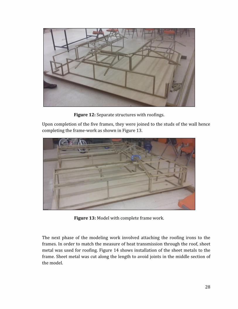
7.0 Model Construction ............................................................................................................ 26
7.1 Materials used .................................................................................................................................... 26
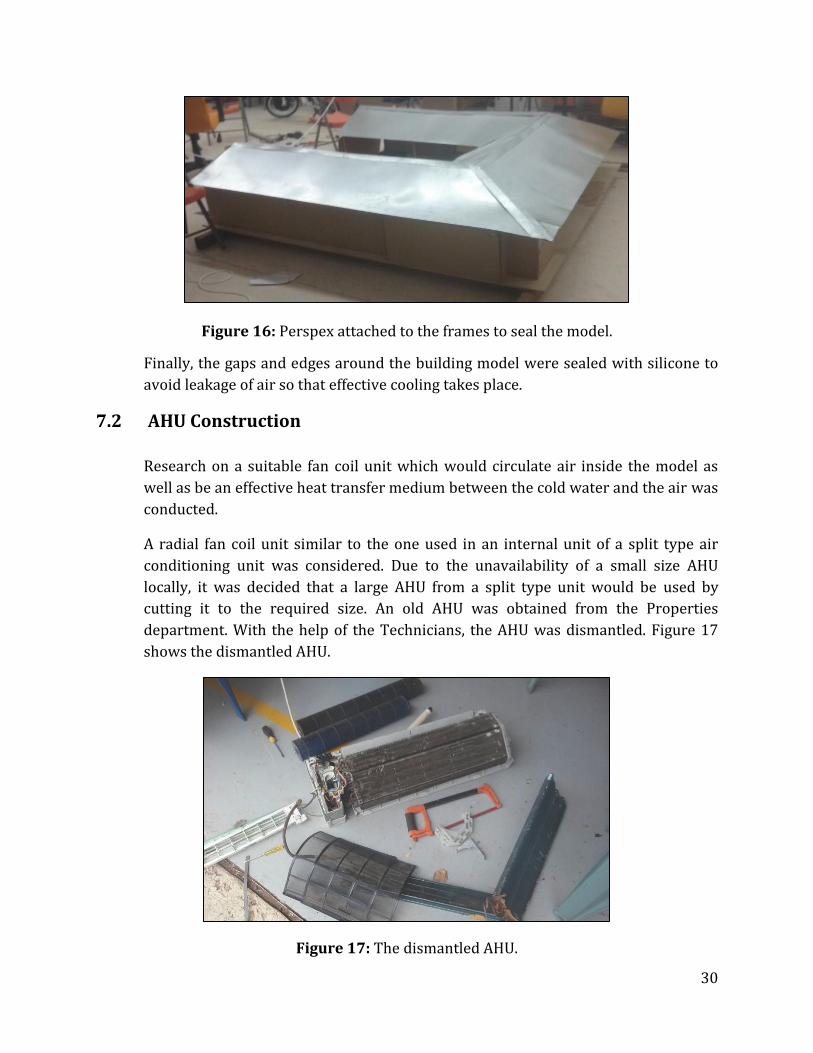
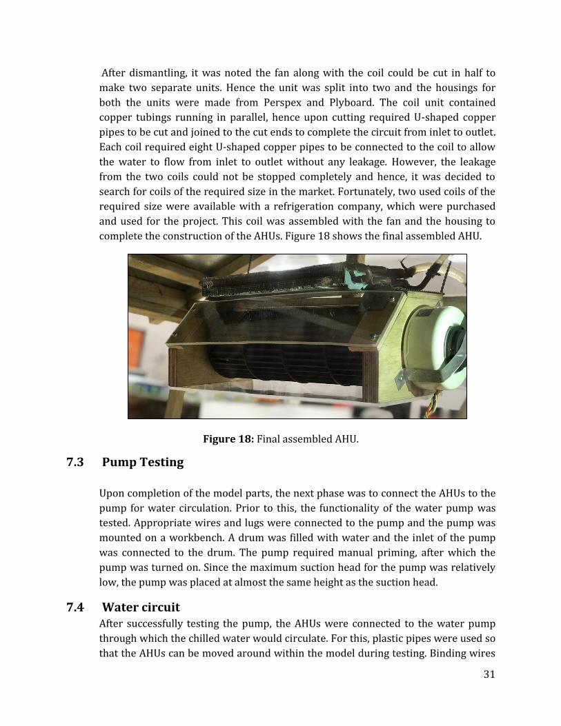
7.2 AHU Construction ............................................................................................................................. 30
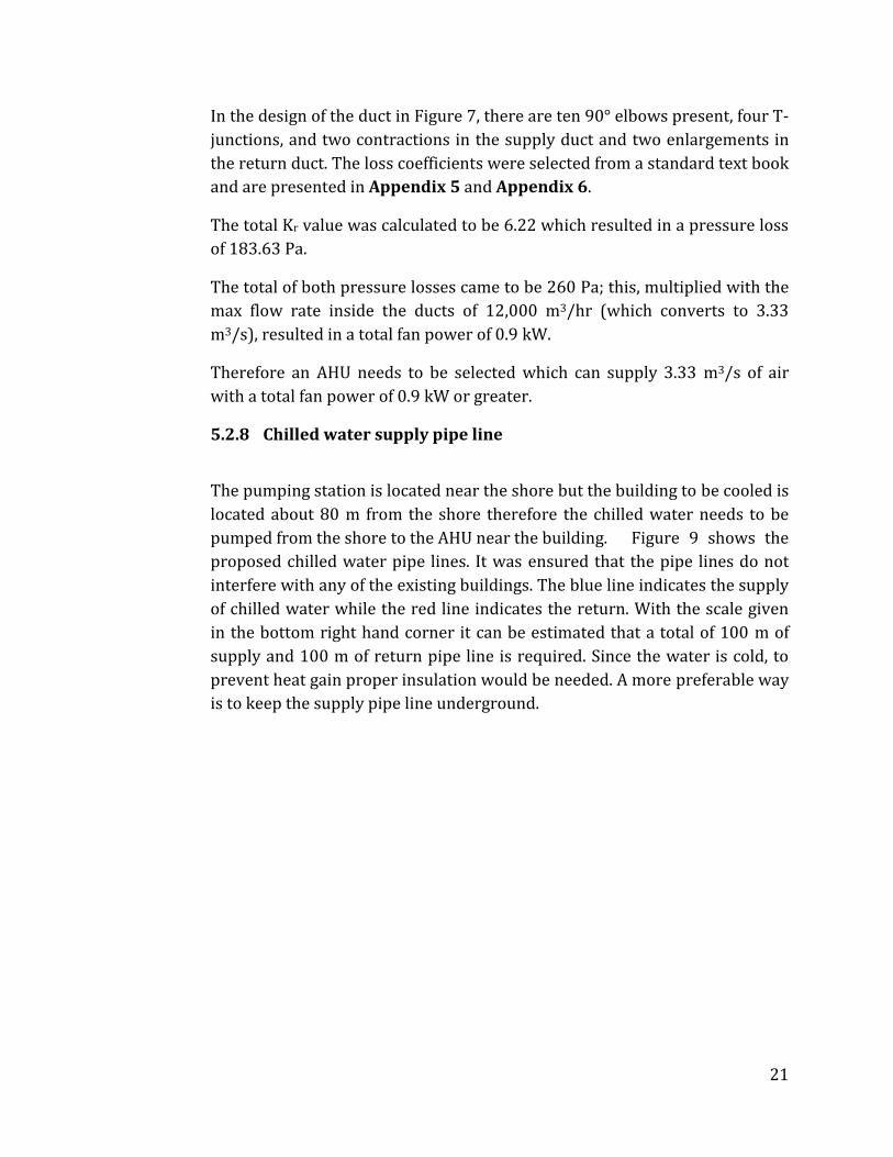
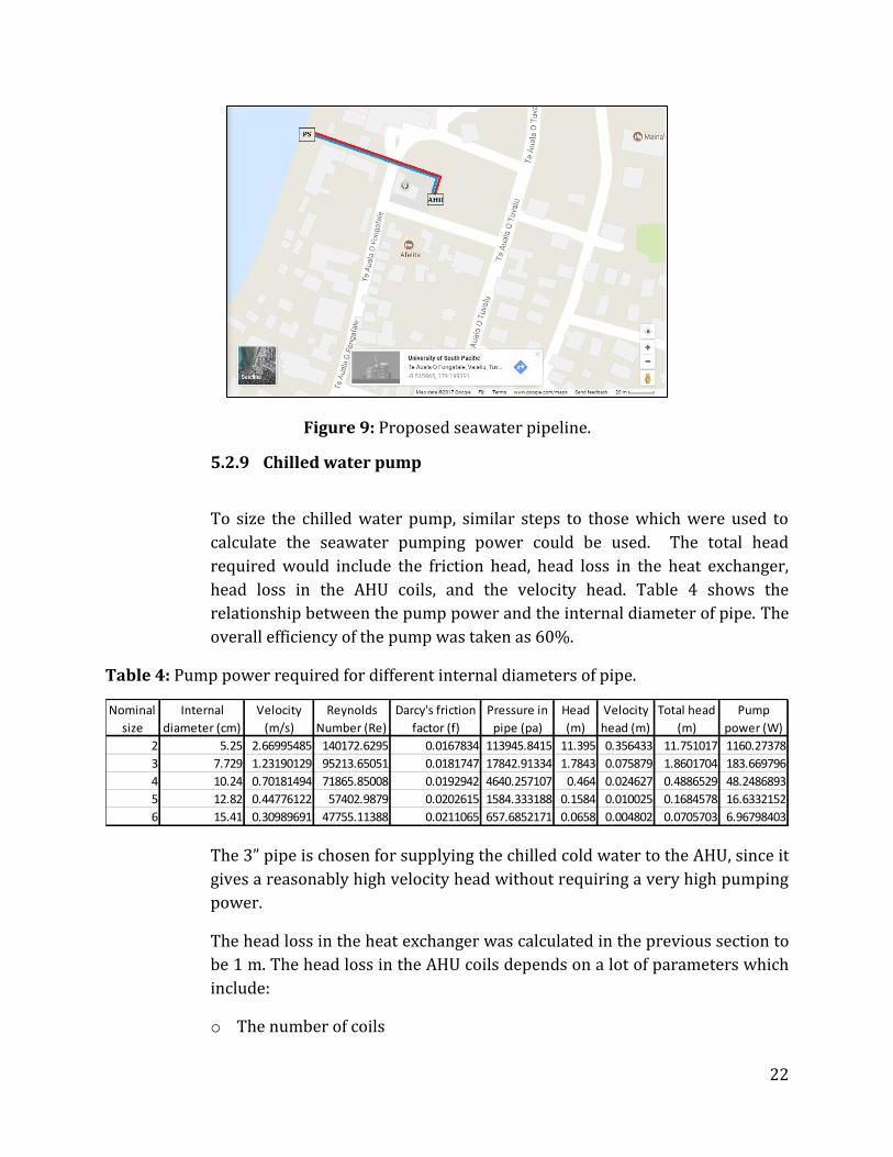
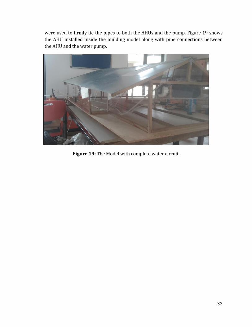
7.4 Water circuit ....................................................................................................................................... 31
8.0 Model Testing ....................................................................................................................... 33
8.1 Leak testing of the of the pipe works and the AHU coils ................................................... 33
8.2 Heating the model ............................................................................................................................ 33
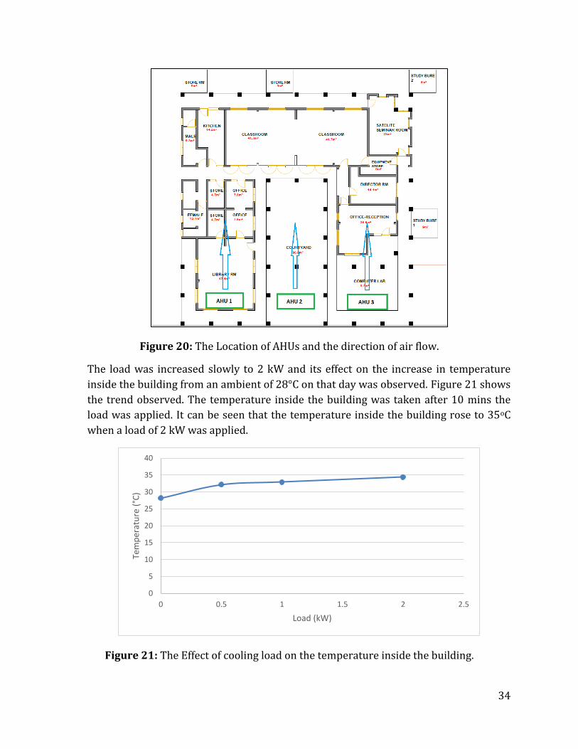
8.3 Positioning of the two AHU’s ....................................................................................................... 33
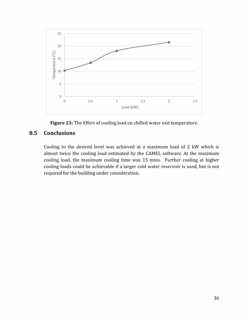
8.4 Effect of cooling load on the time to reach 22°C inside the building ............................ 35
9.3 Payback Period .................................................................................................................................. 38
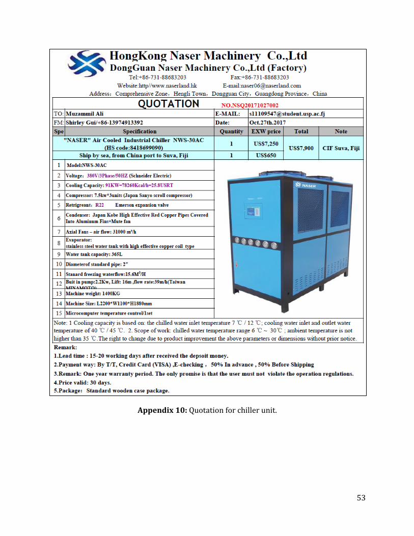
9.3.1 Scenario 1: Comparison with central water chiller system..................................... 39
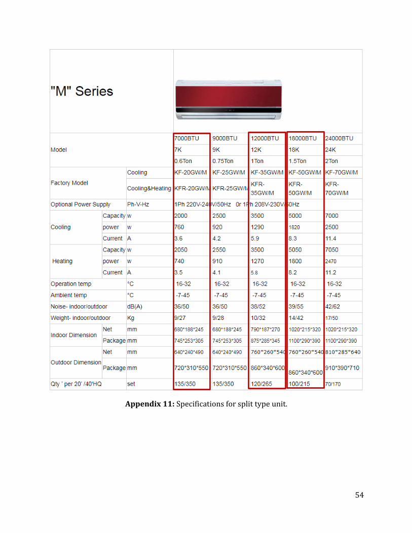
9.3.2 Scenario 2: Comparison with split type AC system .................................................... 39
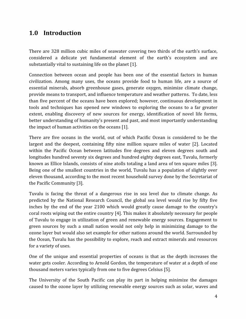
provide means to transport, and influence temperature and weather patterns. To date, less
than five percent of the oceans have been explored; however, continuous development in
tools and techniques has opened new windows to exploring the oceans to a far greater
extent, enabling discovery of new sources for energy, identification of novel life forms,
better understanding of humanity’s present and past, and most importantly understanding
the impact of human activities on the oceans [1].
There are five oceans in the world, out of which Pacific Ocean is considered to be the
largest and the deepest, containing fifty nine million square miles of water [2]. Located
within the Pacific Ocean between latitudes five degrees and eleven degrees south and
longitudes hundred seventy six degrees and hundred eighty degrees east, Tuvalu, formerly
known as Ellice Islands, consists of nine atolls totaling a land area of ten square miles [3].
Being one of the smallest countries in the world, Tuvalu has a population of slightly over
eleven thousand, according to the most recent household survey done by the Secretariat of
the Pacific Community [3].
Tuvalu is facing the threat of a dangerous rise in sea level due to climate change. As
predicted by the National Research Council, the global sea level would rise by fifty five
inches by the end of the year 2100 which would greatly cause damage to the country’s
coral roots wiping out the entire country [4]. This makes it absolutely necessary for people
of Tuvalu to engage in utilization of green and renewable energy sources. Engagement to
green sources by such a small nation would not only help in minimizing damage to the
ozone layer but would also set example for other nations around the world. Surrounded by
the Ocean, Tuvalu has the possibility to explore, reach and extract minerals and resources
for a variety of uses.
One of the unique and essential properties of oceans is that as the depth increases the
water gets cooler. According to Arnold Gordon, the temperature of water at a depth of one
thousand meters varies typically from one to five degrees Celsius [5].
The University of the South Pacific can play its part in helping minimize the damages
caused to the ozone layer by utilizing renewable energy sources such as solar, waves and
5
wind. One of the ways to support this initiative is to commence the use of deep sea cold
water to air condition the Campuses of the University.
A seawater air conditioning (SWAC) system utilizes a water pump to suck water from deep
sea for cooling. Seawater is pumped inland and circulated through a heat exchanger. The
heat exchanger has another loop of fresh water circulating through it as well. Upon arriving
to the heat exchanger the seawater gains heat from the fresh water and is discharged to the
ocean at a lesser depth. Upon giving off heat to the seawater, the fresh water becomes cool
and is passed to the Air Handling Units (AHU) installed in the buildings. The AHU contains a
fan coil unit which operates similar to the internal unit of a conventional air conditioning
unit. The fan draws air past the coils and fins of the unit where heat from the air is
transferred to the water inside the coil, in turn making the air cool. This air is than supplied
to the building and the cycle continues.
6
2.0 Objectives
o To check the feasibility of implementing a SWAC system in Tuvalu.
o Estimation of the total cooling load for the USP Tuvalu campus using CAMEL
software.
o Determine the sea depth at which sea water is cold enough for sufficient
cooling applications.
o To choose a suitable SWAC system for the cooling of the above-mentioned
campus.
o Use of dimensional analysis to scale down the necessary components for
modelling.
o To construct a scaled-down model of the campus and construct it in the
Mechanical Engineering Laboratory of USP.
o To estimate the sizing requirements for all the components of the SWAC
system.
7
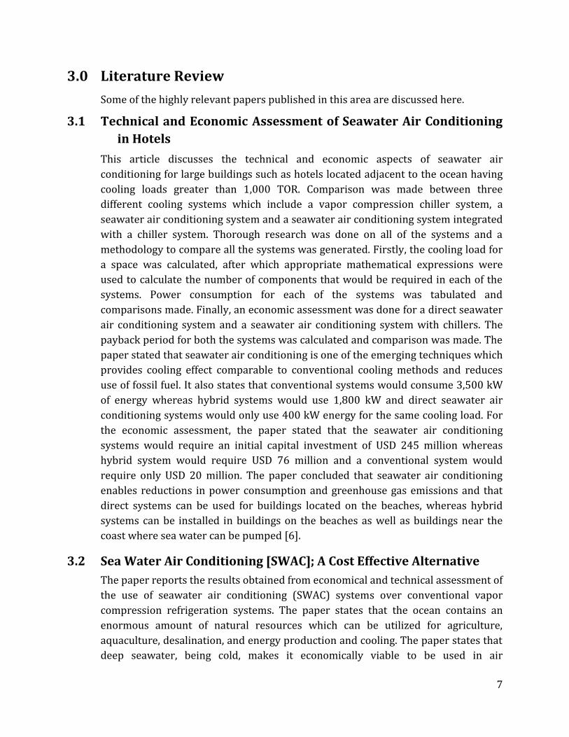
3.0 Literature Review
Some of the highly relevant papers published in this area are discussed here.
3.1 Technical and Economic Assessment of Seawater Air Conditioning
in Hotels
This article discusses the technical and economic aspects of seawater air
conditioning for large buildings such as hotels located adjacent to the ocean having
cooling loads greater than 1,000 TOR. Comparison was made between three
different cooling systems which include a vapor compression chiller system, a
seawater air conditioning system and a seawater air conditioning system integrated
with a chiller system. Thorough research was done on all of the systems and a
methodology to compare all the systems was generated. Firstly, the cooling load for
a space was calculated, after which appropriate mathematical expressions were
used to calculate the number of components that would be required in each of the
systems. Power consumption for each of the systems was tabulated and
comparisons made. Finally, an economic assessment was done for a direct seawater
air conditioning system and a seawater air conditioning system with chillers. The
payback period for both the systems was calculated and comparison was made. The
paper stated that seawater air conditioning is one of the emerging techniques which
provides cooling effect comparable to conventional cooling methods and reduces
use of fossil fuel. It also states that conventional systems would consume 3,500 kW
of energy whereas hybrid systems would use 1,800 kW and direct seawater air
conditioning systems would only use 400 kW energy for the same cooling load. For
the economic assessment, the paper stated that the seawater air conditioning
systems would require an initial capital investment of USD 245 million whereas
hybrid system would require USD 76 million and a conventional system would
require only USD 20 million. The paper concluded that seawater air conditioning
enables reductions in power consumption and greenhouse gas emissions and that
direct systems can be used for buildings located on the beaches, whereas hybrid
systems can be installed in buildings on the beaches as well as buildings near the
coast where sea water can be pumped [6].
3.2 Sea Water Air Conditioning [SWAC]; A Cost Effective Alternative
The paper reports the results obtained from economical and technical assessment of
the use of seawater air conditioning (SWAC) systems over conventional vapor
compression refrigeration systems. The paper states that the ocean contains an
enormous amount of natural resources which can be utilized for agriculture,
aquaculture, desalination, and energy production and cooling. The paper states that
deep seawater, being cold, makes it economically viable to be used in air
8
conditioning through a SWAC system. The paper presents a case study on a resort
called “Sahl-Hasheesh”, located 18 km south of Hurghada in Egypt. A HVAC Load
explorer program was used to calculate the cooling load for the hotel. Site maps
along with Bathymetry charts were then used to design a pipeline schematic for
seawater suction. Appropriate mathematical expressions were then used to size all
the necessary components for the system. Numerical programs were then used to
determine the optimum seawater piping network considering the capital
expenditure, electricity usage for suction, and head loss. An economic analysis using
simple payback method and net present value technique was also done to calculate
the payback period for the SWAC system. Finally, an economic assessment was also
done on a hybrid system which would include a SWAC system integrated with
auxiliary chillers. The auxiliary chillers would be controlled by a programmable
logic controller (PLC) and would only operate if the SWAC system fails to provide
adequate cooling. The paper concluded that a SWAC system is feasible for cooling
loads exceeding 5,000 TOR, hence appropriate for “Sahl-Hasheesh” [7].
3.3 Study of Water Cooling Schemes for Commercial Air-Conditioning
Applications
This paper reviews the performance of an evaporative air conditioning system
operating under the weather conditions of Hong Kong and the economic impact of
modifying an existing evaporative air conditioning unit to a fresh water cooling
tower system in a commercial building. The paper also sheds light on
implementation of seawater district cooling schemes. Firstly, the necessary data for
one year for an existing building were used to simulate operation of an evaporative
air conditioning system using TRNSYS program. Necessary data from a Building
Management System (BMS), which records operation data for air conditioning
systems, were used to simulate electricity consumption for all the plants. All of this
data were then used with appropriate mathematical expressions to calculate the life
cycle cost and the payback period. Finally, the paper outlines the necessary process
path for implementation of a district cooling system (DCS) which includes grouping
nearby buildings together, calculating the total load for individual districts through
the use of cooling load simulation tools such as CARRIER software, and using
appropriate mathematical expressions to size necessary components. The paper
also states that air conditioning in commercial buildings consumes 50-60% of the
total electrical load, hence it is absolutely necessary to consider application of
water-cooled technologies. The paper concludes that modification of an existing air-
cooled air conditioning system to water-cooled AC system is technically as well as
economically practical. [8].
9
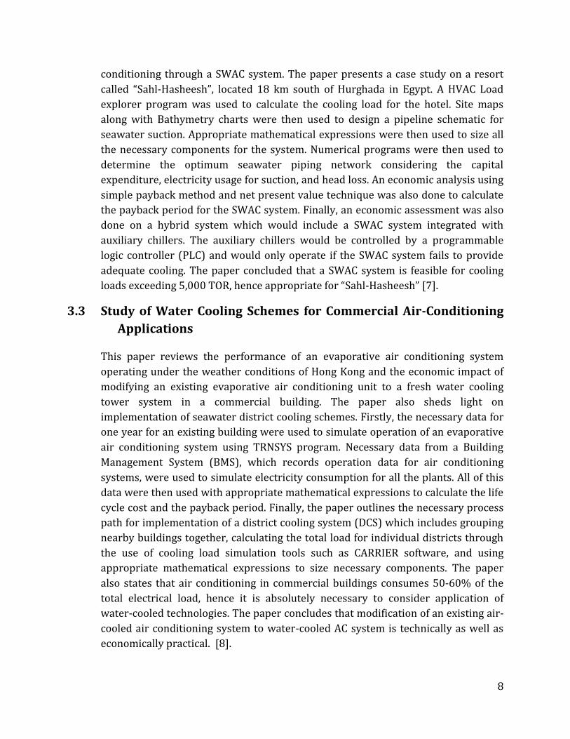
4.0 Methodology Figure 1 shows the flow chart of the methodology undertaken to complete this project. The
feasibility study, load calculation and system sizing were completed in the first phase while
system scaling, seawater temperature measurement, model construction, testing, and
economic analysis were completed in the second phase, and details of each are provided in
sections 6.0, 7.0, 8.0, and 9.0 of this report.
Figure 1: Steps undertaken to complete this project.
FeasibilityStudy
•Acquiring necessary data which includes a Bathymetry chart for Tuvalu and building site plan.•Using the data obtained to check if the building is reasonably close to the ocean and availability of
cold water at reasonable depth. •Measurement of seawater temperature at different depths using a CTD probe.
Cooling Load Calculations
•Acquiring necessary data which includes building blueprints and the climatic weather condition chart for Tuvalu.
•Using CAMEL load calculation software to calculate the total cooling load for the campus.
System
Sizing
•Using the appropriate mathematical models and the cooling load to size necessary components for the seawater air-conditioning system for USP Tuvalu campus.
System Scaling
•Using an appropriate scaling ratio to scale down the building dimensions to a suitable size for construction at the Mechancial Engineering Workshop.
•Using dimensional analysis to scale down the ready-sized components to model size.•Scaling down the cooling load to the model size.
Model Construction
•Construction of a fully operational system according to the dimensions obtained in system scaling.
Testing
•Applying the scaled down load to the model and testing the model for functionality.
Economic Analysis
•Conducting an economic analysis to determine if a seawater air-conditioning system can be implemented.
10
5.0 Cooling Load Estimation and System Sizing
This chapter presents the first phase of the project. The work in the first phase included
thorough research on SWAC systems and their components. After research, the next phase
of the project was data collection. Necessary project data such as the Bathymetry chart for
Tuvalu, building blue-prints, and weather data for Tuvalu were collected. The seawater
temperatures at different depths were measured using a CTD probe. After successful data
collection, the load calculation software, CAMEL, was used to calculate the total cooling
load for USP Tuvalu Campus. Finally, appropriate mathematical expressions along with the
calculated cooling load were used to size the major components of a SWAC system for USP
Tuvalu Campus.
5.1 Load Calculation using CAMEL For calculation of the total cooling load for the campus the following steps were
followed:
5.1.1 CAMEL Software
The CAMEL software allows cooling load calculation when all the geometric
details and year-round ambient conditions are fed in to it.
5.1.2 Data Collection
Data collection involved obtaining the following:
o Building Blue-print – These contained necessary details and
dimensions for the building which were to be fed in to the program.
Later, the actual measurements of the dimensions were performed
during the visit to Tuvalu.
o Google map – To identify the building’s north direction since it was
not available on the floor plan.
o Weather chart for Tuvalu – To input climatic design conditions for
Tuvalu.
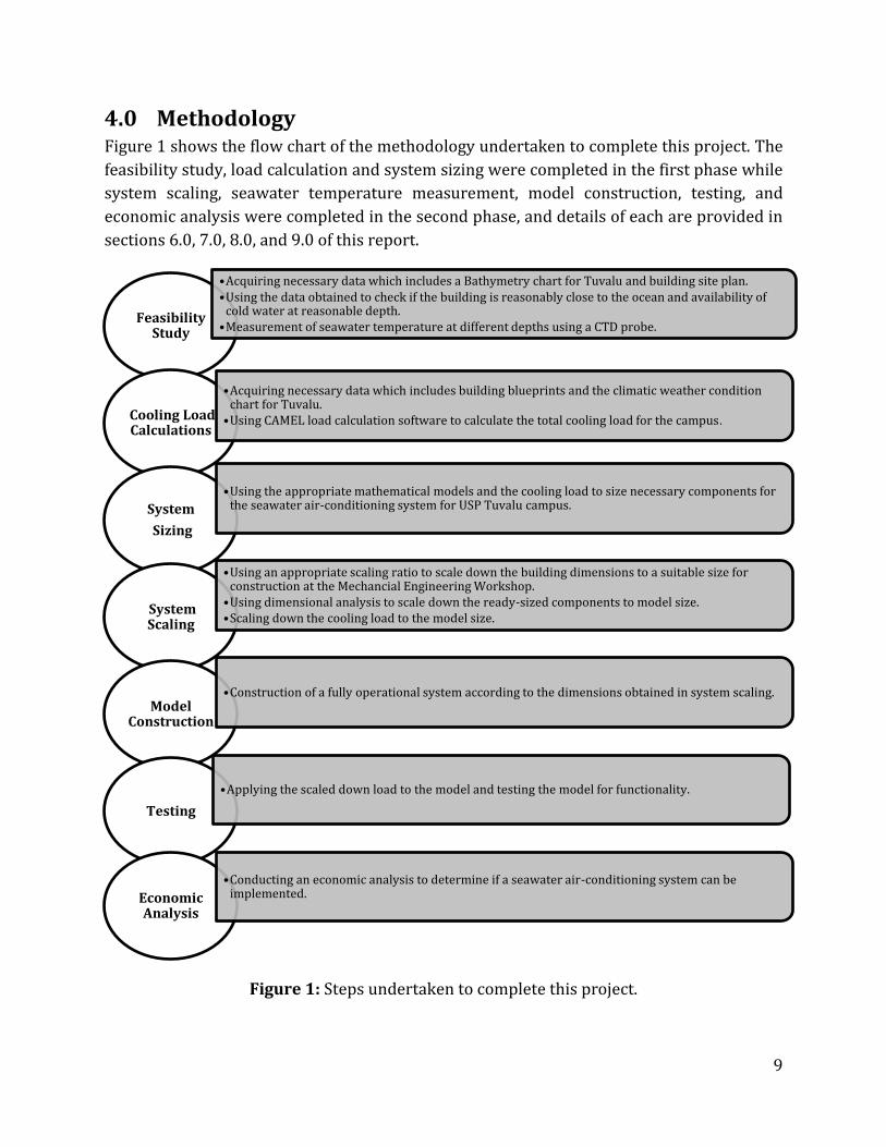
5.1.3 CAMEL Project Screens
CAMEL Program contains two series of tabs which require data input. The
Project tab has a total of six screens in it which require general project
information and information which could be cross-referenced while
inputting data for individual zones in the AHU screen tabs. All the necessary
details in the project screen were fed in according to the data obtained.
Figure 2 shows details of one of the tab’s in-project screens.
11
Figure 2: Project tab for user-defined general project details.
5.1.4 CAMEL AHU Screens
Since the building contains a total of eight rooms which require cooling, each
air handling unit was dedicated to one room so that individual rooms would
have their own control system, since some rooms would require cooling for
only certain hours whereas rooms like the satellite room and the computer
lab may require longer cooling hours. Details for each room were filled in the
individual AHU tab and necessary information from the project screen tabs
were cross referenced. Figure 3 shows details of all the AHU tabs that
required information input.
12
Figure 3: General AHU tab showing all the sections which required information input.
5.1.5 View Screen
The view screen shows details of the results from the program. After
validation of all the details, the program was run and the total cooling load
for the building was estimated. The primary plant results tab, given below as
Figure 4, show the total cooling load for the building. Details for individual
AHU units were also available on the view screens which include the
breakdown of loads – for example, the total sensible and latent heat that will
be generated in each room along with details of load due to people giving-off
heat, external heat, and the heat from equipment and lighting. Graphs for the
entire plant were also available on the view screen which showed the grand
total heat versus time plot.
Figure 4: Primary plant results tab.
5.1.6 Result
The total cooling load was estimated to be 117 kW, as can be seen from the
Fig. 4.
13
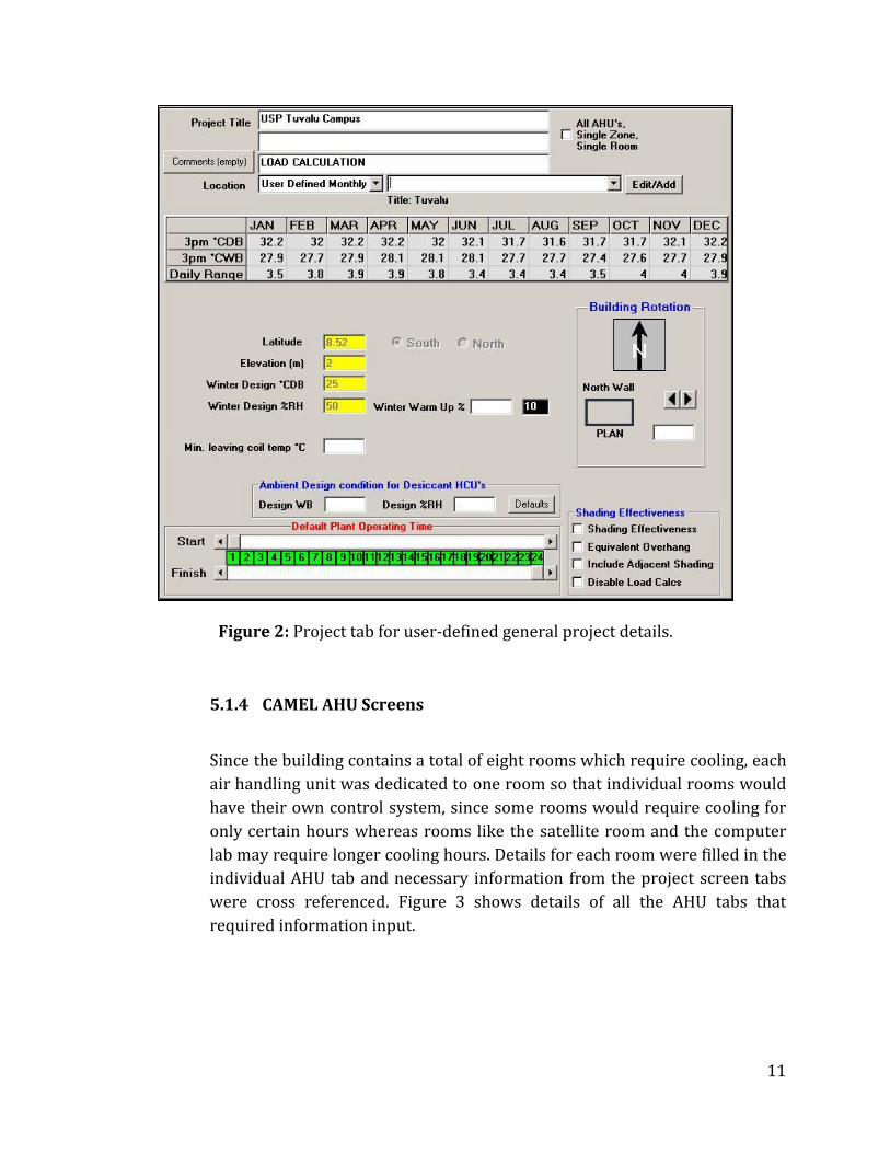
5.2 System Sizing Calculations
Once the total cooling load of the USP Tuvalu campus was calculated, a safety factor
of 12% was applied, which was rounded off to 132 kW. All the components sized
hereafter take into consideration this new load. A simple SWAC system, shown in
Figure 45, having a seawater pump, a heat exchanger, and a chilled water pump was
selected for the campus.
Figure 5: Layout of the recommended SWAC system
5.2.1 Energy balance
There were two energy balances that were applied. Firstly an energy balance
was done between the chilled water supply and the total cooling load of the
building. Then an energy balance was done between the chilled water supply
and seawater supply in the heat exchanger. The purpose of doing these
energy balances was to calculate the mass flow rate of each of the supply
pipelines. Since the heat transfer equations aside from the mass flow rate
variable contained another variable, which was the temperature difference
before and after heat absorption, different scenarios were considered where
the temperature difference was altered and its effect on mass flow rate was
seen.
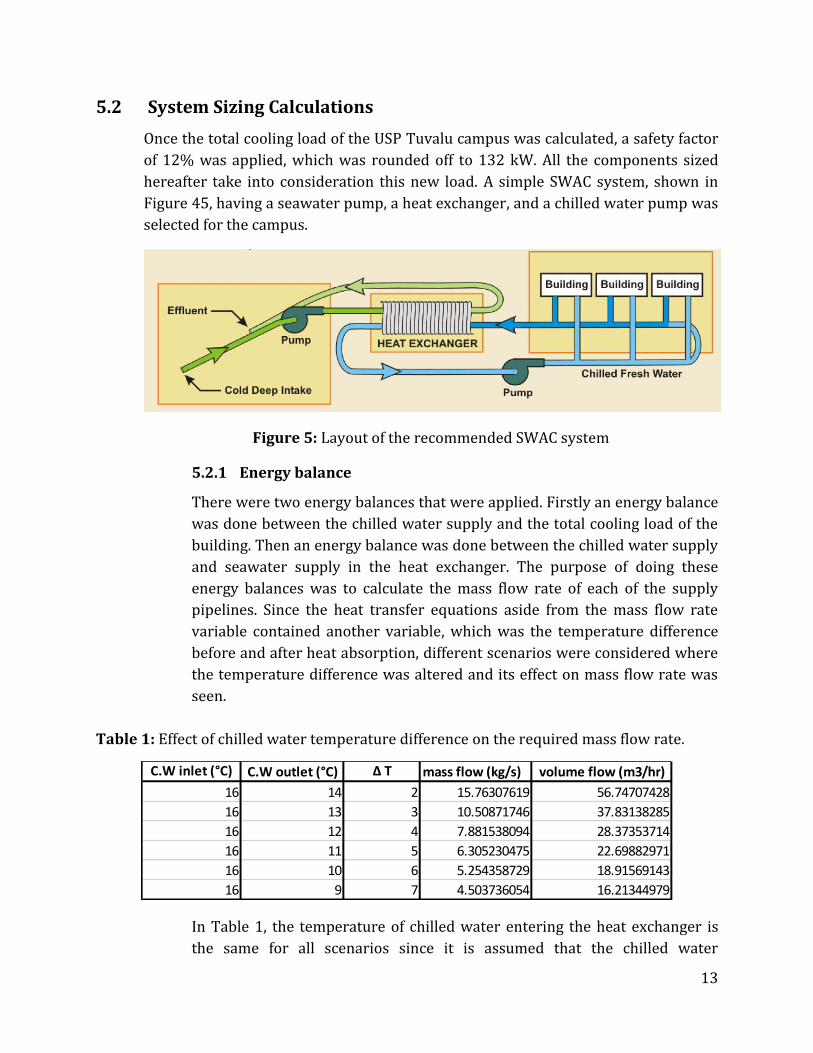
Table 1: Effect of chilled water temperature difference on the required mass flow rate.
In Table 1, the temperature of chilled water entering the heat exchanger is
the same for all scenarios since it is assumed that the chilled water
C.W inlet (°C) C.W outlet (°C) ∆ T mass flow (kg/s) volume flow (m3/hr)
16 14 2 15.76307619 56.74707428
16 13 3 10.50871746 37.83138285
16 12 4 7.881538094 28.37353714
16 11 5 6.305230475 22.69882971
16 10 6 5.254358729 18.91569143
16 9 7 4.503736054 16.21344979
14
temperature would be at 16°C while leaving the building (re-entering the
heat exchanger).
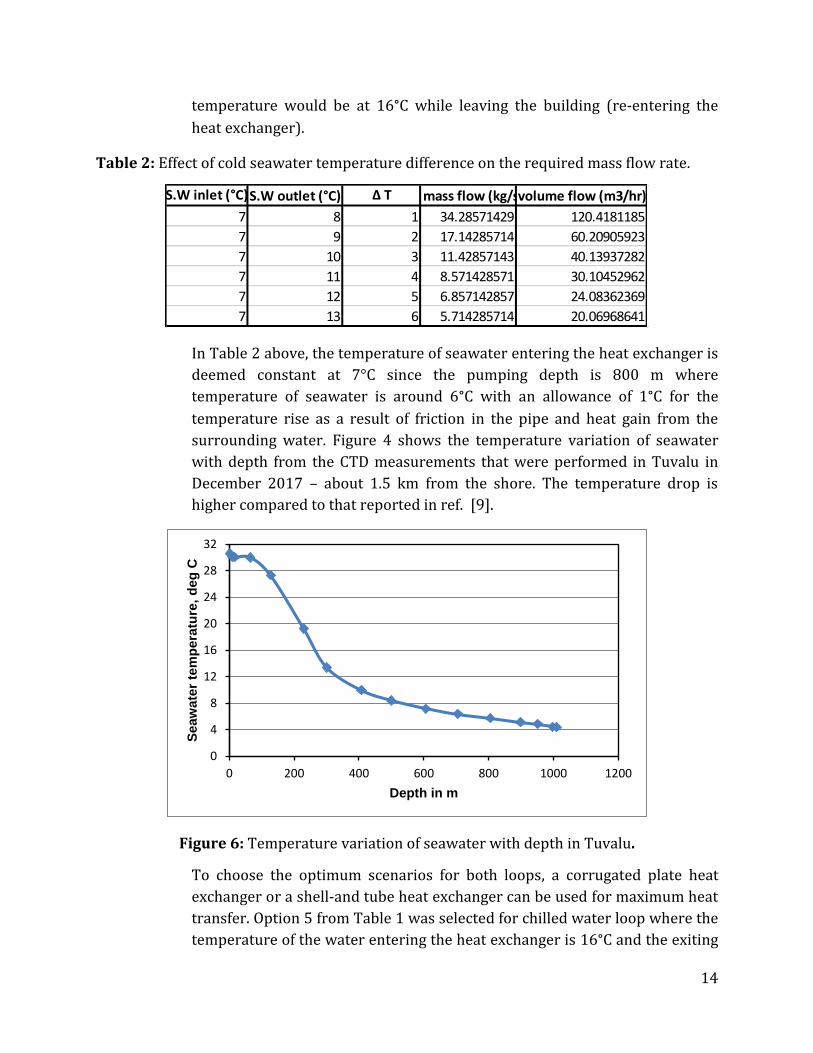
Table 2: Effect of cold seawater temperature difference on the required mass flow rate.
In Table 2 above, the temperature of seawater entering the heat exchanger is
deemed constant at 7°C since the pumping depth is 800 m where
temperature of seawater is around 6°C with an allowance of 1°C for the
temperature rise as a result of friction in the pipe and heat gain from the
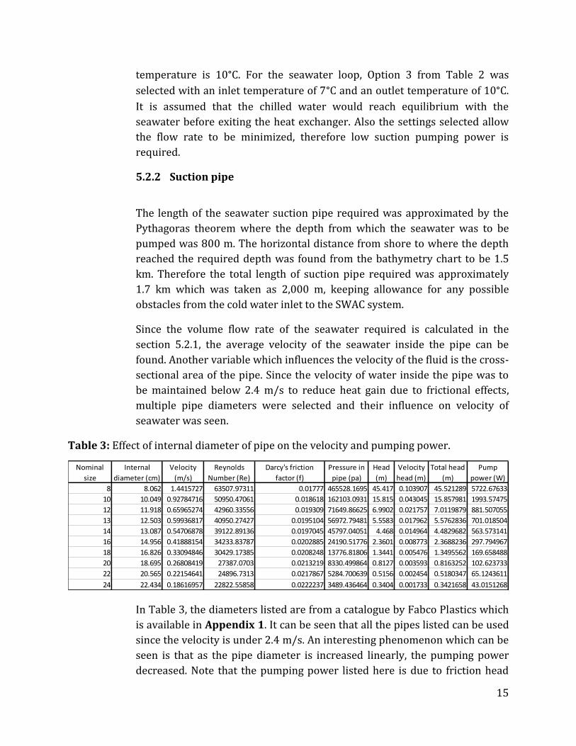
surrounding water. Figure 4 shows the temperature variation of seawater
with depth from the CTD measurements that were performed in Tuvalu in
December 2017 – about 1.5 km from the shore. The temperature drop is
higher compared to that reported in ref. [9].
Figure 6: Temperature variation of seawater with depth in Tuvalu.
To choose the optimum scenarios for both loops, a corrugated plate heat
exchanger or a shell-and tube heat exchanger can be used for maximum heat
transfer. Option 5 from Table 1 was selected for chilled water loop where the
temperature of the water entering the heat exchanger is 16°C and the exiting
S.W inlet (°C)S.W outlet (°C) ∆ T mass flow (kg/s)volume flow (m3/hr)
7 8 1 34.28571429 120.4181185
7 9 2 17.14285714 60.20905923
7 10 3 11.42857143 40.13937282
7 11 4 8.571428571 30.10452962
7 12 5 6.857142857 24.08362369
7 13 6 5.714285714 20.06968641
0
4
8
12
16
20
24
28
32
0 200 400 600 800 1000 1200
Seaw
ate
r te
mp
era
ture
, d
eg
C
Depth in m
15
temperature is 10°C. For the seawater loop, Option 3 from Table 2 was
selected with an inlet temperature of 7°C and an outlet temperature of 10°C.
It is assumed that the chilled water would reach equilibrium with the
seawater before exiting the heat exchanger. Also the settings selected allow
the flow rate to be minimized, therefore low suction pumping power is
required.
5.2.2 Suction pipe
The length of the seawater suction pipe required was approximated by the
Pythagoras theorem where the depth from which the seawater was to be
pumped was 800 m. The horizontal distance from shore to where the depth
reached the required depth was found from the bathymetry chart to be 1.5
km. Therefore the total length of suction pipe required was approximately
1.7 km which was taken as 2,000 m, keeping allowance for any possible
obstacles from the cold water inlet to the SWAC system.
Since the volume flow rate of the seawater required is calculated in the
section 5.2.1, the average velocity of the seawater inside the pipe can be
found. Another variable which influences the velocity of the fluid is the cross-
sectional area of the pipe. Since the velocity of water inside the pipe was to
be maintained below 2.4 m/s to reduce heat gain due to frictional effects,
multiple pipe diameters were selected and their influence on velocity of
seawater was seen.
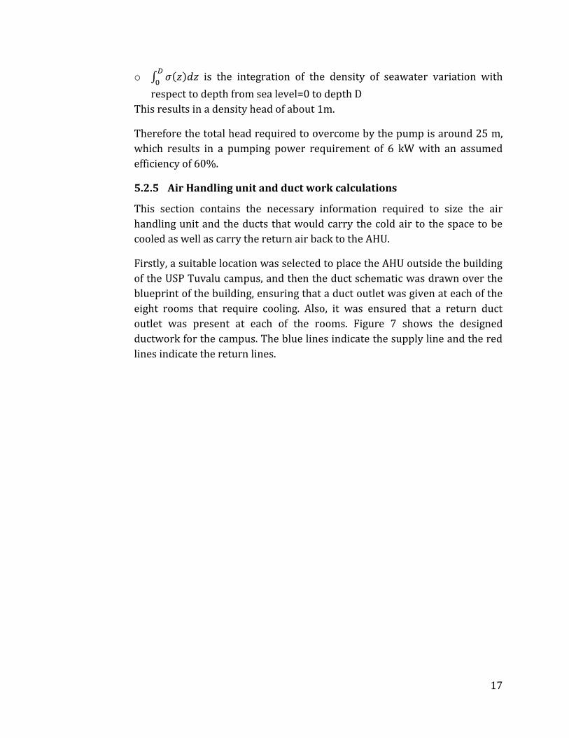
Table 3: Effect of internal diameter of pipe on the velocity and pumping power.
In Table 3, the diameters listed are from a catalogue by Fabco Plastics which
is available in Appendix 1. It can be seen that all the pipes listed can be used
since the velocity is under 2.4 m/s. An interesting phenomenon which can be
seen is that as the pipe diameter is increased linearly, the pumping power
decreased. Note that the pumping power listed here is due to friction head