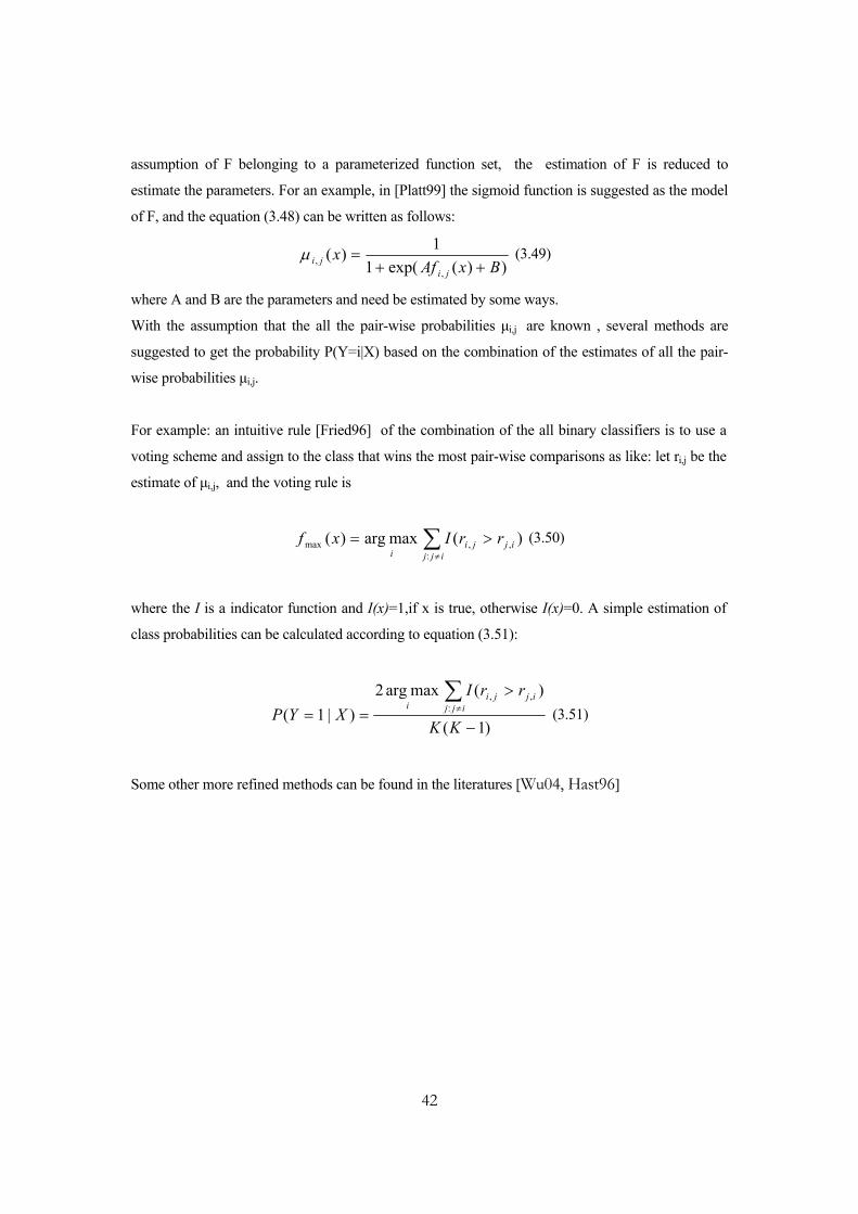
POUR L'OBTENTION DU GRADE DE DOCTEUR ÈS SCIENCES PAR Master of Engineering, Chinese Academy of Science, Beijing, Chine de nationalité chinoise acceptée sur proposition du jury: Lausanne, EPFL 2006 Prof. J. R. Mosig, président du jury Dr M. Mattavelli, directeur de thèse Prof. C. Bornand, rapporteur Prof. M. Kunt, rapporteur Prof. R. Rabenstein, rapporteur FEATURE EXTRACTION OF MUSICAL CONTENT FOR AUTOMATIC MUSIC TRANSCRIPTION Ruohua ZHOU THÈSE N O 3638 (2006) ÉCOLE POLYTECHNIQUE FÉDÉRALE DE LAUSANNE PRÉSENTÉE LE 17 OCTOBRE 2006 À LA FACULTÉ DES SCIENCES ET TECHNIQUES DE L'INGÉNIEUR Laboratoire de traitement des signaux 3 SECTION DE GÉNIE ÉLECTRIQUE ET ÉLECTRONIQUE
Transcript
POUR L'OBTENTION DU GRADE DE DOCTEUR ÈS SCIENCES
PAR
Master of Engineering, Chinese Academy of Science, Beijing, Chinede nationalité chinoise
acceptée sur proposition du jury:
Lausanne, EPFL2006
Prof. J. R. Mosig, président du juryDr M. Mattavelli, directeur de thèse
Prof. C. Bornand, rapporteurProf. M. Kunt, rapporteur
Prof. R. Rabenstein, rapporteur
feature extraction of musical content for automatic music transcription
Ruohua ZHOU
THÈSE NO 3638 (2006)
ÉCOLE POLYTECHNIQUE FÉDÉRALE DE LAUSANNE
PRÉSENTÉE LE 17 OCTOBRE 2006
à LA FACULTÉ DES SCIENCES ET TECHNIQUES DE L'INGÉNIEUR
Laboratoire de traitement des signaux 3
SECTION DE GÉNIE ÉLECTRIQUE ET ÉLECTRONIQUE
ii
ACKNOWLEDGMENTS
First of all, I wish to express my genuine gratitude and respect to Dr Marco Mattavelli, my
director of the thesis. Time passes so quickly, it has been more than five years since I at the first
time wrote to Dr Mattavelli and looked for a chance to pursue PhD. I also remember that he
kindly welcomed me in his office and introduced me to other colleagues when I came to EPFL
for the first time. I admire his broad interdisciplinary expertise. Dr Mattavelli spent much time
for instructing my experiment and provided me many valuable suggestions for my thesis. He also
shows me some creative ideas for future research.
I wish to express my special gratitude to Dr Giorgio Zoia. We have worked together for nearly
five years. Dr Zoia is my project leader and also gives me instruction for my research work. He
is a very excellent project manager and creates a nice work environment for me. I never forget
that he once gave me much help. Dr Zoia introduced me into the challenging field of automatic
music analysis. He spent much time on helping me improve my thesis. Thank Dr Zoia very much
for his continuous support and encouragement during past several years.
I am very grateful to Prof. Daniel Mlynek. As the director of our laboratory, he makes it possible
for me to work and study here. He once spent his precious time on checking my PhD work and
gave me guidance. He also gave me more time for my PhD work.
I would like to express my whole-hearted gratitude to Prof. Murat Kunt, Prof. Rudolf Rabenstein,
Prof. Cedric Bornand, Professor Auke Jan Ijspeert, who do me the honor of accepting to take
part in the jury of my thesis. As the director of Signal Processing Institute, Prof. Murat Kunt
creates a nice academic atmosphere for us. Prof. Rudolf Rabenstein once provided me useful
suggestions for my PhD work. When working in STILE project, Prof. Cedric Bornand gave me
much encouragement. Professor Auke Jan Ijspeert kindly accepted to be president of the jury for
my oral examination.
I would like to thank Mack Vincent for his help in accomplishing the abstract of French version.
I also grateful to my colleagues: Beilu Shao, Aleksandar Simeonov, Robert Lluis Gracia, Massimo Ravasi, Graziano Varotto and Christophe Clerc, Nicolas Scaringella. And thank all the
former and present colleagues in LTS3.
iii
Finally, I am greatly grateful to my parents, sister and brother for their support and
encouragement.
iv
TABLE OF CONTENTS
ACKNOWLEDGMENTS ................................................................................ II
TABLE OF CONTENTS................................................................................IV
LIST OF FIGURES......................................................................................VIII
LIST OF TABLES...........................................................................................X
1.4 Main Results of the Thesis............................................................................................................3
1.5 Organization of the Thesis............................................................................................................7
CHAPTER 2 TIME-FREQUENCY ANALYSIS FOR MUSIC SIGNAL: STATE OF THE ART ..................................................................................... 9
4.2 Resonator Time-Frequency Image for Musical Signals ..........................................................45 4.2.1 Energy and Frequency-difference Spectrum of RTFI........................................................49
4.3 Discrete Resonator Time-Frequency Image .............................................................................52 4.3.1 Definition of Discrete RTFI....................................................................................................52 4.3.2 Implementation of Discrete RTFI .........................................................................................53 4.3.3 An Example of Discrete RTFI ...............................................................................................61 4.3.4 Multiresolution Fast Implementation of Discrete RTFI ....................................................62
4.3.4.1 Proposed Multiresolution Fast Implementation..........................................................62 4.3.4.2 Comparison with other Multiresolution Fast Implementations...............................65
5.2 Reviews of Related Work .............................................................................................................68 5.2.1 Time-Frequency Processing...................................................................................................69 5.2.2 Detection Function Producing ...............................................................................................70
6.2 Reviews of Related Work ...............................................................................................................101 6.2.1 Auditory Model of Pitch Perception .........................................................................................101 6.2.2 Blackboard System......................................................................................................................104 6.2.3 Machine-learning Methods ........................................................................................................105 6.2.4 Iterative Methods ........................................................................................................................106 6.2.5 Estimation Using Instrument Model.........................................................................................108
6.3 Problems in Polyphonic Pitch Estimation.....................................................................................109
CHAPTER 7 A NEW POLYPHONIC PITCH ESTIMATION METHOD: METHOD I ...................................................................................................... 113
7.1 System Overview ..............................................................................................................................113
7.2 Time-frequency Processing Based on the RTFI Analysis ...........................................................114
7.4 Making Preliminary Estimation of Possible Multiple Pitches....................................................116
7.5 Cancelling Extra Pitches by Checking Harmonic Components.................................................119
7.6 Judging the Existence of the Pitch Candidate by the Spectral Smoothing Principle..................120
CHAPTER 8 A NEW POLYPHONIC PITCH ESTIMATION METHOD COMBINING SVM AND SIGNAL PROCESSING: METHOD II.................... 123
8.1 System Overview .................................................................................................................................123
8.2 Motivation for Selecting SVM Instead of Neural Network............................................................124
8.3 Input Vectors and SVM Training .....................................................................................................124
9.2 Training/Tuning Database and Test Database................................................................................130
9.3 Test Results on the Test Database 1 (Polyphonic Mixtures)..........................................................133 9.3.1 Test Results of Method I on Polyphonic Mixtures ..................................................................133 9.3.2 Test Results of Method II on Polyphonic Mixtures ................................................................138
vii
9.4 Automatic Music Transcription Systems .........................................................................................143
9.5 Results on the Real Music Excerpts ..................................................................................................148
CHAPTER 10 CONCLUSION AND FUTURE WORK .................................. 151
10.1 Conclusion..........................................................................................................................................151 10.1.1 An Original Time-Frequency Analysis Tool: Resonator Time-Frequency Image (RTFI).................................................................................................................................................................151 10.1.2 Music Onset Detection ..............................................................................................................151 10.1.3 Polyphonic Pitch Estimation....................................................................................................152
10.2 Future Work ......................................................................................................................................153 10.2.1 Special-Purpose SVM Polyphonic Estimator ........................................................................153 10.2.2 Using Temporal Features for Polyphonic Pitch Estimation ................................................153
Table 5.2 : Result of Energy Detection Algorithm with Best parameter ……………………………………………….84
Table 5.3 : Result of Energy Detection Algorithm with Global Best parameter ………………………………………..85
Table 5.4 : Result of Pitch-Based Detection Algorithm with Global Fitting parameter………………………………....92
Table 5.5: Result for Pluck String ………………………………………………………………………………….......94
Table 5.6: Result for Solo Winds…..…………………………………………………………………………………...95
Table 5.7: Result for Piano……..…..…………………………………………………………………………………....95
Table 5.8: Result for Solo Brass………………………………………………………………………………………...96
Table 5.9: Result for Sustained String…………………………………………………………………………………..96
Table 5.10: Result for Complex Music…………………………………………………………………………………..97
Table 6.1: Small Integer Ratio and Note Interval ……………………………………………………………………...111
Table 7.1: Deviation between approximation and ideal value ………………………………………………………....124
Table 9.1 Test Database 2-(Real Music Excerpts from Music CDs)…………………………………………………...133
Table 9.2 : Test Result on the Test Database 2 (Real Music Excerpts) ………………………………………………. 148
Table 9.3: Recall and Precision of Different Methods on Testing Real Polyphonic Music Excerpts…………………...149
Table 9.4: NERof Different Methods on Testing Polyphonic Mixtures (Avoiding Deletions )………………………. 150
Table 9.5: NERof Different Methods on Testing Polyphonic Mixtures (Avoiding Insertions )………………………..150
xi
ABBREVIATIONS
AES Adjusted energy spectrum
CWM Common western music
CWT Continuous wavelet transform
DPES Difference pitch energy spectrum
ERB Equivalent rectangular bandwidth
ERM Empirical risk minimization
FDTF Frequency-dependent time-frequency transform
FFT Fast Fourier transform
KKT Karush-Kuhn-Tucker
MIDI Musical Instrument Digital Interface
MIREX Music Information Retrieval Evaluation Exchange
NPES Normal pitch energy spectrum
NER Note error rate
PES Pitch energy spectrum
PWD Pseudo Wigner-Distribution
QP Quadratic programming
RBF Radial basis function
RTFI Resonator time-frequency image
SACF Summary autocorrelation function
STFT Short Time Fourier Transform
SNR Signal-to-noise ratio
SVM Support vector machine
TDNN Time-delay neural networks
TFR Time-frequency representation
TPP Time-pitch probability
WT Wavelet Transform
WVD Wigner-Ville Distribution
xii
ABSTRACT
The purpose of this thesis is to develop new methods for automatic transcription of melody and
harmonic parts of real-life music signal. Music transcription is here defined as an act of
analyzing a piece of music signal and writing down the parameter representations, which indicate
the pitch, onset time and duration of each pitch, loudness and instrument applied in the analyzed
music signal.The proposed algorithms and methods aim at resolving two key sub-problems in
automatic music transcription: music onset detection and polyphonic pitch estimation. There are
three original contributions in this thesis.
The first is an original frequency-dependent time-frequency analysis tool called the Resonator
Time-Frequency Image (RTFI). By simply defining a parameterized function mapping frequency
to the exponent decay factor of the complex resonator filter bank, the RTFI can easily and
flexibly implement the time-frequency analysis with different time-frequency resolutions such as
ear-like (similar to human ear frequency analyzer), constant-Q or uniform (evenly-spaced) time-
frequency resolutions. The corresponding multi-resolution fast implementation of RTFI has also
been developed.
The second original contribution consists of two new music onset detection algorithms: Energy-
based detection algorithm and Pitch-based detection algorithm. The Energy-based detection
algorithm performs well on the detection of hard onsets. The Pitch-based detection algorithm is
the first one, which successfully exploits the pitch change clue for the onset detection in real
polyphonic music, and achieves a much better performance than the other existing detection
algorithms for the detection of soft onsets.
The third contribution is the development of two new polyphonic pitch estimation methods.
They are based on the RTFI analysis. The first proposed estimation method mainly makes best of
the harmonic relation and spectral smoothing principle, consequently achieves an excellent
performance on the real polyphonic music signals. The second proposed polyphonic pitch
estimation method is based on the combination of signal processing and machine learning. The
basic idea behind this method is to transform the polyphonic pitch estimation as a pattern
recognition problem. The proposed estimation method is mainly composed by a signal
processing block followed by a learning machine. Multi-resolution fast RTFI analysis is used as
a signal processing component, and support vector machine (SVM) is selected as learning
xiii
machine. The experimental result of the first approach show clear improvement versus the other
state of the art methods.
Keywords: Signal processing, music transcription, onset detection, polyphonic pitch estimation
xiv
RESUME
Cette thèse aborde le sujet de la transcription musicale, que l'on définit ici comme le fait
d'analyser le signal d'un morceau de musique, et d'en tirer une représentation paramétrique qui
indique le ton, l'instant de l'attaque, la durée de la note, sa force et l'instrument utilisé dans le
signal musical analysé.
De nouvelles méthodes de transcription de la mélodie et des parties harmoniques d'un signal
musical, tel qu'on en trouve dans la vie réelle, en résultent. Les algorithmes et les méthodes
proposées sont axées sur la résolution de deux sous-problèmes clés dans la transcription de la
musique: la détection de l'attaque et l'estimation des tons polyphoniques. Il y a trois apports
inédits dans cette thèse:
Le premier est un outil d'analyse temps-fréquence: le RTFI (pour Resonator Time-Frequency
Image). En définissant simplement une fonction paramétrée faisant correspondre une fréquence
au facteur exponnentiel de declin du groupe de filtres complexes du résonnateur, le RTFI peut
servir à implémenter facilement l'analyse temps-fréquence, avec différentes résolutions du
domaine temps-fréquence, telles que celle de l'oreille humaine, avec un facteur Q constant, ou
encore uniforme (espacée régulièrement). Une implémentation rapide avec plusieurs résolutions
simultanées a également été développée.
Deux nouveaux algorithmes de détection de l'attaque constituent le deuxième apport: l'un basé
sur l'énergie et l'autre sur le ton. Celui basé sur l'énergie se comporte bien sur de fortes attaques.
Celui basé sur le ton est le premier à exploiter correctement le changement de ton dans la
détection d'attaque d'une musique polyphonique réelle, et offre de bien meilleurs résultats que
les autres algorithmes existants, quant il s'agit de détecter des attaques douces.
Enfin, deux nouvelles méthodes d'estimation des tons polyphoniques sont proposées: la
première, basée sur l'analyse RTF, exploite au mieux la relation harmonique et le principe du
lissage spectral. Elle fournit par conséquent d'excellentes performances quand elle est appliquée
à des signaux de musiques polyphoniques réelles. La seconde est basée sur une combinaison de
traitement de signal et d'apprentissage de la machine. L'idée fondamentale de cette méthode est
de transformer l'estimation de tons polyphoniques en un problème de reconnaissance de
xv
modèles. L'analyse RTFI rapide avec plusieurs résolutions simultanées sert au traitement du
signal et l'apprentissage de la machine est géré par SVM (Support Vector Machine). Les
résultats des essais effectués avec cette méthode montrent de claires améliorations de l’état de
l’art.
Liste des mots-clefs :
Traitement du signal, transcription de la musique, détection de notes, estimation de hauteur
polyphonique
1
C h a p t e r 1
INTRODUCTION
1.1 Definition of Automatic Music Transcription Music transcription is here defined as an act of analyzing a piece of music signal and writing down
the parameter representations, which indicate the pitch, onset time and duration of each pitch,
loudness and instrument applied in the analyzed music signal. Automatic music transcription is a
process to convert an acoustical waveform into a musical notation (such as the traditional western
music notation) by computer programming. In most cases automatic transcription of common
monophonic music can be considered as a matured filed, however the computational transcription of
polyphonic music has less relative success. Transcription of polyphonic music is a very difficult task
for the average human without training, however human can improve their transcription ability by
learning. Skilled musicians are able to transcribe polyphonies with much better performance than
computational transcription system can achieve in current research phases. The automatic music
transcription is a critical step for some higher level music analysis tasks such as melody extraction,
rhythm tracking, and harmony analysis.
1.2 Objectives The purpose of this thesis is to develop new methods for automatic transcription of melody and
harmonic parts of real-life music signal. The proposed algorithms and methods aim at resolving two
key sub-problems in automatic music transcription: music onset detection and polyphonic pitch
estimation. The music signal is often considered as the succession of the discrete acoustic events.
The term music onset detection refers to the detection of the instant when a discrete event begins in
acoustic signal. The term polyphonic pitch estimation refers to the estimation of possible pitches in
the polyphonic music signal that several music notes may occur simultaneously.
1.3 Motivations The music consists of some basic elements. These are rhythm, melody, harmony, and timbre. The
aim of this thesis is to extract two important parameters: note onset time and polyphonic pitch. As
shown in Figure 1.1, the extraction of the both parameters plays an essential role in a music analysis.
2
The extracted onset time of music notes can be used to chiefly determine rhythm. The extracted
multiple pitches of music notes can be primarily employed for the detection of melody and harmony.
Melodic lines are sequences of notes over time, and harmony is determined by the relationship
between the multiple simultaneously occurring pitches of music notes.
Because the extraction of note onset time and polyphonic pitch is a fundamental stage of analyzing
the basic elements of music signals, it can be utilized to support broad music applications. As shown
in the Figure 1.1, except the automatic music transcription itself, the possible applications include
content-based music retrieval, automatic music summarization, interactive music system, low-bitrate
compression coding for music signal and so on. Multimedia music applications are nowadays
rapidly moving from simple content related scenarios to more complex and sophisticated domains
including content, interaction, related descriptions and annotations, item identification. The creation
of huge databases coming from both restoration of existing analog content and new digital content is
Figure 1.1 Essential Role of the extracted parameters: Onset Time and Polyphonic Pitch in Music Analysis
3
requiring more and more reliable and fast tools for content analysis and description, to be used for
searches, content queries and interactive access. In the case of content-based music retrieval,
automatic onset and harmonic information extraction is crucial. Not only it is interesting to build
measures of harmonic similarity between musical excerpts, but it can further help some other kind of
analysis such as rhythm or instrument detection by finding onset time points where such events or
instrument note starts are more likely to be observed. . Another interesting point that is gaining
importance in the domain is the automatic control of signal processing parameters according to
content features and builds some music interactive systems. Another possible application of the
extraction of polyphonic pitch is to assist for the low-bitrate coding for music signal. The MPEG-4
Structured Audio coding provides new methods for low-bitrate storage. In a framework of
Structured Audio coding, automatic music transcription and music synthesis play chief role.
1.4 Main Results of the Thesis The main three original contributions of this thesis can be summarized as follows:
1) An original frequency-dependent time-frequency analysis tool has been proposed and
formalized: the Resonator Time-Frequency Image (RTFI).
Music signal is time-varying, and most of the music related tasks need a joint time-frequency
analysis. An important time-frequency representation (TFR) is the Wigner-Ville Distribution (WD)
which satisfies a number of desirable mathematical properties and provides high time-frequency
resolution. However, the serious cross term interference in the WD prevents it from the practical
application. A number of existing TFRs can be considered as the smooth version of WD to reduce
the cross term interference. According to their covariance property, these existing TFRs can be
categorized into several main classes such as the Cohen’s class of time-frequency distributions, the
Affine class of time-frequency distributions. For example, in the commonly-used TFRs for music
analysis, the spectrogram (STFT analysis) is a particular example of the Cohen’s class of time-
frequency distribution, and the scalogram (wavelet analysis) belongs to the Affine class of time-
frequency distribution.
The Cohen’s class of time-frequency distributions perform the time-frequency analysis with a
uniform time-frequency resolution in the time-frequency plane (“uniform analysis”), on the other
hand the Affine class of time-frequency distributions have the “constant-Q” time-frequency
resolution (“constant-Q analysis”). Most of the current existing TFRs show similar limitations, and
their time-frequency resolutions are either uniform or “constant-Q”. However, it is well known that
4
time-frequency resolution of human ear frequency analyzer is neither uniform nor “constant-Q”.
This motives me to develop a more general and flexible class of TFRs whose time-frequency
resolutions are not limited in the uniform or “constant-Q” analysis. I extend the spectrogram into a
broader class of TFRs and make the window function dependent on analysis frequency. Base on this
idea, I propose and formulate a particular time-frequency representation: the Resonator Time-
Frequency Image (RTFI) for music signal analysis. The RTFI is implemented by the one-order
complex IIR-filter bank, so it is computation-efficient. By simply defining a parameterized function
mapping frequency to the exponent decay factor of the complex resonator filter bank, the RTFI can
easily and flexibly implement the time-frequency analysis with different time-frequency resolutions
such as ear-like (similar to human ear frequency analyzer), constant-Q or uniform (evenly-spaced)
time-frequency resolutions. The corresponding multi-resolution fast implementation of RTFI has
also been developed. The practical application examples of RTFI analysis are the proposed music
onset detection algorithms and polyphonic pitch estimation methods. In all these algorithms and
methods, the RTFI become the common time-frequency analysis tool.
2) Two music onset detection algorithms have been proposed and developed: Energy-based
detection algorithm and Pitch-based detection algorithm.
The note onsets may be classified into “soft” or “hard” onsets according to slow or fast transitions
between the two successive notes in the analyzed music signal. The note transition with hard onset is
accompanied with the sharp change in energy, and the note transition with soft onset shows a
gradual change. Based on the RTFI analysis, I propose an energy-based onset detection algorithm
which is simple and performs very well on the detection of hard onsets. However, the detection of
soft onset has been proved to be very difficult task, because the real-life music signal often contains
the noise and vibration associated with frequency and amplitude modulation. The energy-change in
the vibration probably surpasses the energy-change of soft onset, and this makes it very hard to
distinguish the true onsets from the vibration only based on the energy-change clue.
Pitch change is the most salient clue for note onset detection of the music signal with soft onset. On
the one hand, there exist many onset detection systems that use energy change and/or phase change
as the source of information, on the other hand, only few pitch-based onset detection systems exist.
One important reason for this is that pitch-tracking itself is an challenging task.
The proposed Pitch-based detection algorithm uses RTFI analysis and produces a pitch energy
spectrum that makes the pitch change more obvious; and then makes best use of pitch change clues
5
to separate the music signal into transient and stable part, and finally searches the possible note
onsets only in the transient part. This method greatly reduced the false positives that caused by the
salient energy-change in the stable part of the music note, and greatly improve the detection
performance on the music signal with many soft onsets or vibration.
Both of the energy-based and pitch-based detection algorithms have been tested on broad real-life
music excerpts and the test results are encouraging. Especially, for the detection of the soft onsets,
the proposed Pitch-based detection algorithm achieves a much better performance compared to the
other existing onset detection algorithms.
3) Two polyphonic pitch estimation methods have been proposed and developed: polyphonic
pitch estimation method I and polyphonic pitch estimation method II. Polyphonic pitch estimation is
a very challenging task because of the wide pitch range, much variety of the spectral structures of
the different instrument sound and the coinciding harmonic components frequently occurring in the
polyphonic sound.
The proposed polyphonic pitch estimation method I mainly makes best of the harmonic relation and
spectral smoothing principle. The harmonic relation means that the ratio between frequency
components of a real monophonic music note and its fundamental frequency is integer or nearly
integer. The spectral smoothing principle refers to the fact that the corresponding harmonic spectral
envelop of a real monophonic music note often is gradually change. The proposed method I first
produces the energy spectrum by RTFI analysis, and then uses the harmonic grouping principle to
transform the RTFI energy spectrum into the pitch energy spectrum. The preliminary pitch
candidates are estimated by picking the peaks in the pitch energy spectrum. The extraneous
estimations in the pitch candidates are to be cancelled by the spectral smoothing principle. The detail
description of the proposed estimation method I can be found in the Chapter 5.
The proposed polyphonic pitch estimation method II is based on the combination of signal
processing and machine learning. The basic idea behind this method is to transform the polyphonic
pitch estimation as a pattern recognition problem. The proposed estimation method is mainly
composed by a signal processing block followed by a learning machine. Compared to the human
listening system, the signal processing stage is a time-frequency signal analysis tool similar to
cochlear filters, whereas the learning machine plays a role similar to human brain. Multi-
resolution fast RTFI analysis is used as a signal processing component, and support vector machine
6
(SVM) is selected as learning machine. The detail description of the proposed estimation method II
also can be found in the Chapter 5.
Additionally, with the combination of the proposed onset detection algorithms and polyphonic pitch
estimation methods, the real automatic music transcription prototype systems have also been
proposed and developed.
The both proposed polyphonic pitch estimation methods have been tested on the real music excerpts
from the music CDs, clean polyphonic mixtures and the polyphonic mixtures with different level
pink noise. The polyphonic mixtures is produced by the mixing the monophonic samples of 23
different music instrument types. The test results of the both proposed methods are competitive and
encouraging, compared to the existing methods. On the one hand, the proposed method I presents
better overall performance than the proposed method II (SVM). On the other hand, the method II
(SVM) can produce time-pitch probability output, which is useful for some real applications.
7
1.5 Organization of the Thesis This thesis is organized as follows. Chapter 2 summarizes the existing time-frequency analysis
methods and presents their specific advantages and problems in their usages. Chapter 3 has an
introduction of support vector machines. The original work is introduced in the Chapter 4-9. Chapter
4 presents and formalizes an original time-frequency analysis method: the Resonator Time-
Frequency Image (RTFI), which is especially designed for music signal analysis. The corresponding
multi-resolution fast implementation and application examples of RTFI are also introduced. As a
basic time-frequency analysis tool, the RTFI is exploited in the later proposed music onset detection
algorithms (introduced in Chapter 5) and polyphonic estimation methods (introduced in Chapter 6-
9).Chapter 5 presents two proposed music onset detection algorithms: Energy-based detection
algorithm and Pitch-based detection algorithm, and both algorithms employ the RTFI as the time-
frequency analysis tool. Chapter 6-9 proposes two polyphonic pitch estimation methods, Polyphonic
pitch method I and Polyphonic pitch method II. The method I also uses the RTFI as the time-
frequency analysis tool, and time-frequency analysis of method II uses the RTFI multi-resolution
fast implementation (introduced in Chapter 4). Additionally, Chapter 9 presents two real music
transcription systems which combine the proposed polyphonic pitch methods and the music onset
detection algorithms (introduced in Chapter 5). Chapter 10 presents the main conclusions and
discusses the future work.
8
9
C h a p t e r 2
TIME-FREQUENCY ANALYSIS FOR MUSIC SIGNAL: STATE
OF THE ART
2.1 Introduction The classic Fourier Transform is a very useful tool for frequency analysis of a stationary signal that
maintains the same period over an infinite duration time. The Fourier Transform can show if a
frequency component exists, but not tell when the frequency component occurs. The music signal is
time-varying and non-stationary, its frequency components change with time, so music signal
frequency analysis should better be a joint time-frequency analysis, which shows how the signal’s
frequency content evolves in time.
Because of the uncertainty principle, it is impossible for a time-frequency analysis to have both the
best time and frequency resolution at the same time: there is a tradeoff between time and frequency
resolution. To select a suitable time-frequency resolution for a joint time-frequency analysis of the
music signal, there are two different approaches. The first one is to learn more about how human
ear makes a time-frequency analysis by research in audio physiology and psychology, because the
ear has very excellent performance as a music signal processing component (in fact, the auditory
filter bank can be seen as a time-frequency analysis tool that simulates the cochlear function.).
Another one is to learn more about the time-frequency energy density distribution of the most
typical music signals. In the end, both approaches should be considered together to select a suitable
time-frequency analysis.
One commonly-used time-frequency analysis tool is Short Time Fourier Transform (STFT), which
cuts the signal into different slices and calculates the Fourier Transform on each slice to obtain a
local time-frequency analysis. A different approach to get the local time-frequency analysis is the
Wigner distribution, but its non-linearity causes cross interference, and at the same time the
computation cost is very expensive; the above two reasons make Wigner distribution rarely used in
practical applications. Wavelets are of course another alternative way to joint time-frequency
analysis, and moreover they have a constant-Q frequency resolution that is similar to cochlear
frequency resolution distribution at high frequencies, so the wavelet analysis is more adaptable to
10
music signal processing than the STFT, which has the same time-frequency resolution in all the
time-frequency domain; but the wavelet analysis still shows a similar limitation as STFT, as it
always keeps the constant-Q frequency resolution: it can not flexibly set the time-frequency
resolution in the time-frequency domain. On the other hand, the known cochlear filter only has
similar constant-Q frequency resolution at high frequency, and it has a nearly equal frequency
resolution at low frequency. The next sections will review the above mentioned tools in more detail
and present their actual and possible uses in the context of music sound analysis.
2.2 STFT and Spectrogram Fourier Transform and its inverse can transform signals between the time and frequency domains,
and it becomes a very useful tool for stationary signal processing. It can make it possible to view the
signal characteristics either in time or frequency domain, but not to combine both domains. In order
to obtain a joint time-frequency analysis for non-stationary signals, STFT cuts the time signal into
different frames and then perform a Fourier Transform in each frame. The STFT and its power
spectrum named spectrogram, can be defined like in equations (2.1) and (2.2)
∫∞
∞−
−−= τττω ωτdetwftSTFT j)()(),( (2.1)
2),(),( ωω tSTFTtPower = (2.2)
The STFT at time t is the Fourier Transform of a local signal, which is obtained by multiplication of
a signal )(tf and a short window function )( tw −τ centered at time t. When moving the window
along the signal time axis, we can calculate the STFT at different time instants and obtain a joint
time-frequency analysis. Since STFT can be easily and efficiently implemented by fast algorithms
of Fast Fourier Transform (FFT), it and the spectrogram have been early used in speech and music
signal analysis. To construct a STFT, the effective length and shape of the window function is a key
factor to determine the STFT characteristics. The shape of the window function is the first important
factor; the default window is the rectangle widow, which causes the well-known frequency leakage
problem because the signal’s phase discontinuity at the edge of the window. To reduce the
frequency leakage, some other windows are often selected such as the Hanning window. The other
very important factor is the length of the window; the longer the window, the better frequency
resolution the STFT has, but unfortunately at the price of poorer temporal resolution according to
the uncertainty principle. Given a window function )(tw and its Fourier Transform )(ωW , the
11
commonly used measure of the time and frequency resolution is the window’s effective length t∆
and bandwidth ω∆ , defined as in the following formulas:
∫∫ −
=∆dttw
dttwttt 2
22'2
)(
)()( (2.3)
∫∫ −
=∆ωω
ωωωωω
dW
dW2
22'2
)(
)()( (2.4)
where
∫∫=
dttw
dttwtt 2
2
'
)(
)( (2.5)
∫∫=
dtW
dtWt2
2
'
)(
)(
ω
ωω (2.6)
According to the time-bandwidth uncertainty principle, t∆ and ω∆ must meet the following
inequality:
21' ≥∆•∆ tω (2.7)
According to this inequality, the STFT time and frequency resolutions can not be optimal at the
same time, and there is a trade-off to be found between them. To make the (2.7) be an equality the
window must be the Gaussian window.
One can simply transform the definition (2.1) into another equivalent definition as follows [Hlaw92]:
tjtj eettftSTFT ωωγω −−= )))((*)((),( (2.8) or
))(*))((),( tetftSTFT tj γω ω−•= (2.9)
where )()( twt −=γ (2.10)
12
From the formulas (2.8) and (2.9), there exist two different filter bank interpretations for the STFT
as illustrated in the Figure 2.1.
)(tγf(t)
tje ω−
tjet ωγ )(f(t)
tje ω−
The left part of Figure 2.1 shows the STFT implementation by the band pass filter bank; at any angle
frequencyω , first the signal passes through the band pass filter centered at ω and then it is demodulated to zero frequency. The right part of the Figure 2.1 shows the STFT implementation by
a low pass filter; at any angle frequency, first the signal is demodulated to zero frequency and then
passes through the low pass filter.
As described in the definition of STFT at (2.1), the window function is independent from the
frequency ω , so the time-frequency resolution of STFT is the same in all the time frequency plane.
This makes STFT able to have limited application in music signal processing, because the real
music signal processing often needs to provide better time resolution at high frequencies and better
frequency resolution at low frequencies.
2.3 Wavelet Analysis Differently from the case of STFT, the Wavelet Analysis (WT) provides a varying time-frequency
resolution in the time frequency plane. During the last twenty years, the WT has been developed and
explored in many different research fields. The Wavelet Transform (WT) can be defined as the
following formula:
∫∞
∞−
−= ττφτ d
st
sftsWT )(1)(),( * (2.11)
Figure 2.1 Filter bank interpretation of STFT
13
In the equation the Ф* is the conjugate of theФ. As shown by this definition, WT can be described
in terms of the signal’s decomposition over the wavelet )(, τφ ts , which is defined as the dilation and
translation of the mother wavelet )(τφ :
)(1)(, st
sts−
=τφτφ (2.12)
In (2.12), t is the translation factor; s is the scale factor and s/1 is used to normalize the wavelets.
In (2.11), t, s, and τ are continuous variables; this wavelet transform is commonly named the
Continuous Wavelet Transform (CWT). Differently from other transforms such as FT, the wavelet
basis function is not specified. To make the reverse transform possible, the wavelet function must
meet the so-called admission condition:
∫+∞
∞−
Φ +∞<= ωωω
φ dC2)( (2.13)
Where )(ωΦ is the Fourier Transform of the wavelet function )(τφ :
∫+∞
∞−
−=Φ ττφω ωτ de j)()( (2.14)
With the condition (2.13), the signal )(τf can be reconstructed by the inverse transform of CWT
[Cohen96]:
tdstWTsdsf st∫∫
+∞
∞−
+∞= )(),()( ,0 2 τφτ (2.15)
The condition (2.13) also implies the following property of wavelet exists:
0)0()( =Φ=∫+∞
∞−ττφ d (2.16)
Φ(0) is 0, so the wavelet )(τφ should be oscillating. Sometimes another additional requirement, the
so-called regularity condition, is also imposed for some application that need better detect the
singularity of the analyzed signal. The regularity condition of wavelets can be described as follows:
14
0)( =∫+∞
∞−ττφτ dp Np L2,1,0= (2.17)
Under the regularity condition, the values of ),( stWT are influenced by the regularity of the
analyzed signal )(τf and can be used to detect the signal’s local singularity [Cohen96, Mallat98].
Another equal frequency definition of (2.11) is as following:
∫∞
∞−Φ= ωω
πω ω dessFstWT tj)(
2)(),( *
(2.18)
In the (2.18) )(ωF and )(ωΦ are the Fourier Transform of the signal )(τf and the wavelet
function )(τφ respectively, and the ),( stWT can be considered as the filtering result of the signal
by the band pass filter bank. The filter bandwidth in the filter bank increases as the frequency
increases (the scale factor s decreases), but the ratio between bandwidth and centre frequency keeps
constant..
The CWT decomposes the signal into a time-frequency domain according to a continuously varying
scale and translation and represents the signal with high redundancy, so it is reasonable to calculate
the wavelet coefficient at discrete scale and time grids for a more efficient representation. Such a
discrete sampling wavelet transform can been described as follows:
∫∞
∞−= ττφτ dfkjWT st )()(),( ,
* (2.19)
where )(1)(0
00
0
, j
j
jkj ssk
sττφτφ −
= (2.20)
It is common use to select 20 =s and make a dyadic sampling on the frequency axis. The wavelet
transform decompose the one-dimension signal into the 2 dimensions discrete wavelet coefficients.
At this point it is important to consider if such wavelet coefficients give a complete and stable signal
representation.
15
The frame theory is an important mathematics tool to resolve a problem of this kind. A sequence
{ } znn ∈φ in a Hilbert space H is called a frame if and only if there exists two constants 0>≥ AB
such that for all Hf ∈ ,
( ) 222 , fBffAzn
n ≤≤∑∈
φ (2.21)
When AB = , the frame is said to be tight (Mallat98). A frame is invertible and defines a complete
and stable signal representation. If one wants to make the wavelet coefficients an efficient and
invertible representation, a wavelet function sequence need to be a frame. Daubechies derives the
admission and sufficient condition to construct a wavelet frame (Daub92). When a wavelet function
sequence is a tight frame, it is an orthonormal base.
A new multi-resolution theory was formulated in 1989 and this provided also new view for wavelets
[Mallat89]. The main concept is that wavelet analysis can be considered to approximate the
analyzed signal from a coarse approximation to a more detailed approximation.
According to this multi-resolution theory wavelets can be formulated as a sequence of
approximation subspaces { }zjjV
∈of )(2 RL [ Mallat98]:
jj
j VktfVtfZkj ∈−⇔∈∈∀ )2()(,),( 2 (2.22)
,1, jj VVZj ⊂∈∀ + (2.23)
1)2/()( +∈⇔∈ jj VtfVtf (2.24)
},0{lim ==+∞
−∞=+∞→ jj
jjVV I (2.25)
),()(lim 2 RLClosureVj
jj==
∞
−∞=−∞→U (2.26)
16
and there exists a { } znnt ∈− )(ϕ which is a Riesz basis of 0V
One can define that the function nj ,ϕ as follows:
{ } znjj
nj ntt ∈−− −= )2(2)( 2/
, ϕϕ
From the definition it has been proved that nj ,ϕ is also the Riesz basis of the subspace jV and all
nj ,ϕ are collectively called scaling function, which needs to meet the following so-called scaling
equation:
)2()(2)( ntnht −= ∑ ϕϕ (2.27)
Because nj ,ϕ is the Riesz basis of the subspace Vj, so the nj ,ϕ can be an orthonormal or
biorthormal basis of the subspace jV . One can define an approximation operator Aj that
approximates a )(2 RL function f by the basis of subspace Vj. In the case that nj ,ϕ is an orthonormal
function, Aj is expressed as follows:
njzn
njj ffA ,,, ϕϕ∑∈
= (2.28)
In case that )2( ntj −ϕ is biorthormal basis of the subspace Vj, Aj is expressed as follows:
njzn
njj ffA ,,, ϕϕ∑∈
= (2.29)
where nj ,ϕ is a dual scaling function: nmnjmj −= ,0,, , δϕϕ . The dual scaling function also needs
to meet the scaling equation:
)2()(2)( ntnht −= ∑ ϕϕ (2.30)
17
One can derive a wavelet function from the scaling function as follows:
With the assumption that the frequency resolution is predetermined, according to the equation (4.26),
equation (4.31) can be rewritten as follows:
nkmapSamplingFmapSamplingF kkkk
...3,2))((5.0))((5.0 11
=⋅⋅+=⋅⋅− −− ωωωω
(4.32)
If the sampling factor and the starting analysis frequency ω0 are determined, one can determine the
other filter’s centre frequencies ωk, k=2, 3, …n. according to iterative equation (4.32).
As discussed above a way is proposed to determine the sampling rate for frequency-dependent time-
frequency analysis (FDTF), which is implemented by the boxcar filter bank; if FDTF is
implemented by a filter of different shape, a similar approach may still be used by replacing the
56
bandwidth of the filter with an Equivalent Rectangular Bandwidth (ERB), and in this case the
equations (4.31) and (4.26) can be modified as follows:
nkmapB kERk ,...2,1),( == ω (4.33)
nkBBSamplingF ERk
ERkkk ...3,2),(5.0 11 =+⋅⋅=− −−ωω (4.34)
with BER denotes the ERB of the filter.
As mentioned before the commonly-used frequency resolution distribution for music analysis may
be expressed like:
00,)( >≥+= cdcdresolution ωω (4.35)
and the equation (4.33) can be rewritten as like: kERk cdB ω+= , and the following recursive equation
can be derived according to equation (4.34)
,1 HG kk += −ωω (4.36)
with
SampoingFcSamplingFdH
SampoingFcSamplingFcG
⋅−⋅
=⋅−⋅+
=5.01
,5.015.01
To design a discrete FDTF with frequency resolution according to equation (4.35), one can
determine the discrete centered frequencies of the filter bank according to the following formula,
which can be derived from equation (4.36):
HG
GGk
kk −
−+=
11
0ωω (4.37)
As discussed above, this is a proposed general way to determine the centre frequencies of the filter
bank, which is used to implement a discrete FDTF. The RTFI is a special case of the FDTF, and the
RTFI is a FDTF that can be implemented by first-order complex resonator filter bank; of course a
57
discrete RTFI also can use the proposed method to determine the centre frequencies of the complex
resonator bank.
As shown in the discrete RTFI definition in equation (4.25), to implement a discrete RTFI, two steps
are requested: one is to resolve the frequency sampling issue, i.e to determine the centre frequencies
ωm, which can be resolved by the above proposed method. Another issue is to implement the
frequency resolution distribution, i.e. to determine the bandwidth of each filter in the filter bank. The
bandwidth of the first-order complex resonator filter can be set by the value of exponent decay
factor r in its impulse response. As mentioned before the bandwidth is the ERB width, it is
necessary to know how the exponent decay factor determines the ERB bandwidth of the complex
resonator filter. The ERB bandwidth is defined for the continuous filter in (2.45).
The ERB bandwidth is generalized for a digital filter. The ERB bandwidth of a digital filter is
defined. If a continuous filter has the impulse response h(t), and a corresponding digital filter’s
impulse response is the discrete sampling of h(t), then we approximate the digital filter’s ERB width
by the continuous filter.
According to the RTFI definition (4.5 and 4.6), the frequency response of the filter to be
implemented is centered at frequency ωk and can be described as follows:
22
2
))(
(41
1)(
k
k
rff
fH
ωπ
−+
= (4.38)
The filter ERB can be calculated according to the equation (2.45) and the ERB value can be
expressed according angle frequency as follows:
)))(
arctan(5.0)((k
kk
ERk r
rBωωπω += (4.39)
In practical cases, the resonator filter exponent factor is nearly zero, so arctan(ωk/r(ωk)) can be
approximated to 0.5π, and equation (4.39) can be approximated as follows:
πω )( kERk rB = (4.40)
58
If the RTFI resolution distribution is according to the equation (4.35), the formula to determine the
exponent decay factor for the filter in RTFI filterbank-based implementation can be derived from the
equation (4.40) as follows:
πωω /)()( kk cdr += (4.41)
In practical application, one issue is that sometime we wish the center frequencies of the
implementing filters can be predetermined, for example, we wish the center frequencies always
follows a exponent law and make the analysis result can be more conveniently to connect with
western music, in this case, the sampling factor can not be predetermined any more, but we can
calculate the sampling factor from the known frequency resolution parameters and the centre
frequencies according to the relationship equation (4.30), and the calculated sampling factors at
different frequency can provide the frequency sampling rate information . When the centre
frequencies and exponent decay factors of the impulse response of the implementing digital
resonator filters are determined, the z transfer function of the digital resonator filters can be
expressed as the following equation:
1/)(
/
11)(
−+−
−
−−
=ze
ezHsmm
sm
fjr
fr
m ω (4.42)
As analyzed in the continuous RTFI, the RTFI energy spectrum includes the oscillation terms and
need be smoothed by the low-pass filter. We propose a way to get the smoothed discrete RTFI
energy spectrum by a special low pass filter, and for the mth implementing digital resonator filter,
it’s energy spectrum is smoothed by the corresponding low pass filter with the impulse response as
like
nf
rf
r
mLs
m
s
m
eenI)()(
)1(),(ωω
ω−−
−= , (4.43)
and the low pass filter’ s z transfer function can be expressed as follows:
1/
/
11)( −−
−
−−
=ze
ezHsm
sm
fr
frLm (4.44)
59
There exist two reasons to select such a special low pass filter for smoothing the energy spectrum of
the discrete RTRI. First, a important advantage of the RTFI is it’s computation-efficiency, so we
need keep the advantage and the low pass filter’s order need be also small as possible. Secondly, the
impulse responses of the mth resonator filter and the corresponding mth low pass filter for
smoothing the energy spectrum have the equal exponent decay factor, and this makes the energy
spectrum smoothing process still keep a similar time-frequency resolution distribution as defined in
the discrete RTFI. The smoothed energy spectrum of a discrete RTFI at the frequency ωm can be
expressed as follows according to the responses of the implementing resonator filter and it’s
corresponding low pass filter.
),(),()(),( 2mLmRm
SmoothedEnergy nInInsnRTFI ωωω ∗∗= (4.45)
Where the IR and IL is respectively defined in the equation (4.25) and (4.43)
We calculate the frequency-difference spectrum of a discrete RTFI at the frequency ωm and time
point n by the following formula:
Given the values : ,),1(,),( 11 −− +=−+= nnmnnm jbanRTFIjbanRTFI ωω
( )( )
( )( )
<−−++
+−
>−−++
+
=−−
−−
−−
−−
−−
−−
0:arccos(
0:arccos(
),(112
12
122
11
1121
21
22
11
nnnnm
nnnn
nnnns
nnnnm
nnnn
nnnns
mIF
baabifbaba
bbaaf
baabifbaba
bbaaf
nRTFIω
ω
ω (4.46)
In the practical application of the discrete RTFI, we need consider not only computation but also the
memory issue , generally speaking it is impossible and also not necessary to keep all the RTFI
energy spectrum and frequency-difference spectrum at every time sampling point; to reduce the
requirement of the memory to store the RTFI values, we separate the RTFI into different time
frames and calculate the average RTFI values in each time frame, finally the average smoothed
RTFI energy spectrum and frequency-difference spectrum are used to track a time-frequency
character of the music signal. The average RTFI energy spectrum and frequency–difference
spectrum may be expressed as follows:
60
2
1)1(
),(1(),( ∑+−=
=kM
MkimmEnergy nRTFI
MdbkARTFI ωω (4.47)
∑+−=
=kM
MkimFDmFD iRTFI
MkARTFI
1)1(),(1),( ωω (4.48)
Where the M is an integer and M/fs is the duration time of the frame in the average process.
As analyzed in the continuous RTFI, if there exist several sinusoid components in the input signal,
then the corresponding smoothed RTFI energy spectrum may exist a peak along the frequency axis
nearly around the frequency of each sinusoid component. A discrete RTFI can be considered as an
approximated implementation of continuous RTFI, so it is reasonable to consider the discrete RTFI
still almost keeps some basic characters of the continuous RTFI, this also has been testified by a lot
of experiments in our research of performing the time-frequency analysis for music signal by the
discrete RTIFI. In the discrete RTFI, we do not directly find the peak in the smoothed RTFI energy
spectrum, but in the average smoothed RTFI energy spectrum to reduce the memory requirement as
mentioned before, and the process to find the peak value in the average smoothed RTFI energy
spectrum may be expressed as follows:
;:);,(:
))),((),(())),((),((:
aPeakelsekARTFIPeakthen
LkARTFIkARTFIandLkARTFIkARTFIif
mSE
mSEm
SEm
SEm
SE
==
+−>++>
ω
δωωδωω
In the above expressions, the L and δ are the two parameters to define the peak. In the general case,
we set L=1, and the δ can be considers as a threshold that is useful to remove the noise peak. In the
average smoothed RTFI energy spectrum, if the point is not a peak in the frequency axis, its value is
set to the constant a, which is usually set to the minimum of the smoothed RTFI energy spectrum.
Similar to the case in the continuous RTFI frequency-difference spectrum, in the discrete RTFI
average frequency-difference spectrum, if the average frequency-difference ARTFIFD(k, ωm) is
nearly to zero , this means that it is probable that, in the input signal, there exists a sinusoid
component with the frequency ωm at the kth time frame.
61
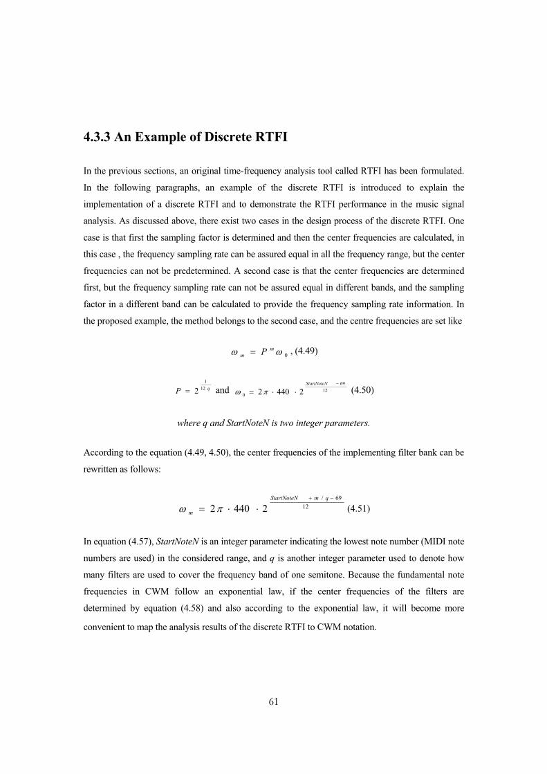
4.3.3 An Example of Discrete RTFI
In the previous sections, an original time-frequency analysis tool called RTFI has been formulated.
In the following paragraphs, an example of the discrete RTFI is introduced to explain the
implementation of a discrete RTFI and to demonstrate the RTFI performance in the music signal
analysis. As discussed above, there exist two cases in the design process of the discrete RTFI. One
case is that first the sampling factor is determined and then the center frequencies are calculated, in
this case , the frequency sampling rate can be assured equal in all the frequency range, but the center
frequencies can not be predetermined. A second case is that the center frequencies are determined
first, but the frequency sampling rate can not be assured equal in different bands, and the sampling
factor in a different band can be calculated to provide the frequency sampling rate information. In
the proposed example, the method belongs to the second case, and the centre frequencies are set like
0ωω mm P= , (4.49)
qP 121
2= and 1269
0 24402−
⋅⋅=StartNoteN
πω (4.50)
where q and StartNoteN is two integer parameters.
According to the equation (4.49, 4.50), the center frequencies of the implementing filter bank can be
rewritten as follows:
1269/
24402−+
⋅⋅=qmStartNoteN
m πω (4.51)
In equation (4.57), StartNoteN is an integer parameter indicating the lowest note number (MIDI note
numbers are used) in the considered range, and q is another integer parameter used to denote how
many filters are used to cover the frequency band of one semitone. Because the fundamental note
frequencies in CWM follow an exponential law, if the center frequencies of the filters are
determined by equation (4.58) and also according to the exponential law, it will become more
convenient to map the analysis results of the discrete RTFI to CWM notation.
62
As already said, there exist four parameters that completely determine a discrete RTFI
implementation, the parameters are the frequency resolution distribution parameters c and d,
sampling factor SamplingF , starting analysis frequency ω0 ; in this example, SamplingF and ω0,
are indirectly set by the two integer parameters q and StartNoteN , so that the centre frequencies
always can meet the definition in equation (4.51). And the relationship between the parameter
SamplingF, the integer parameter q and resolution distribution parameters can be derived. For
convenience of computation, in this example RTFI, the approximated sampling factor A_SamplingF
is derived, which is the sampling factor when the center frequency equals the fundamental frequency
of a CWM note A0 :
)21(440
)21(440_12
1
121
q
q
cdSamplingFA
−
−
+⋅+
−⋅=
π
π (4.52)
After the center frequencies and exponent decay factors of the digital resonator filters are
determined, the example of the discrete RTFI can be implemented according to the method
introduced in the previous section.
The real music application examples in music signal analysis can be found in Chapter 5- 9.
4.3.4 Multiresolution Fast Implementation of Discrete RTFI
4.3.4.1 Proposed Multiresolution Fast Implementation
For practical applications, a multiresolution fast implementation for the discrete RTFI has been
developed. The basic idea is to reduce the redundancy in computation: in some cases it is not
necessary to keep the same sampling frequency of the input for every filter in the filter bank. For the
filters with lower center frequencies, the sampling rate can be decreased. At the same time, because
the main partials of music notes exist according to the exponential law, the high frequency regions
need a lower frequency resolution. This means that a shorter duration signal frame is enough for the
frequency analysis.
63
The block diagram of the proposed implementation is shown in Figure 4.3
LPF 2
Filter Bank
Filter Bank
LPF 2 Filter Bank
S(n)
More
Figure 4.3: Block diagram for the proposed multi-resolution fast implementation
Considering a filter bank without fast implementation, the center frequencies are selected according
to the expression
s
Km
m ff 22 0π
ω = , (m =1,2,….M; N=M/K integer) ( 4.53)
The filter bank is separated into N frequency bands, every frequency band has K filters, and the
center frequencies of the filters in nth frequency band are:
),*)1(( iKn +−ω (i =0,1,2,…K-1) (4.54)
Using the fast implementation, the signal is recursively low pass filtered and down sampled by a
factor 2 from the highest to the lowest frequency band according to the scheme in Figure 4.3. The
signal sampling rate ratio between the nth frequency band and the original sampling rate is
sNn
sn ff −= 2
and according to equation (4.53), the center frequencies of the filters in nth frequency band are
changed as
)*)1(()*)1(()*)1((' 2 iKNiKn
nNiKn +−+−
−+− == ωωω (i =0,1,…K-1)
64
Consequently, all the other n-1 frequency bands use the same filters as the filters in the highest
frequency band.
If the computation cost of one frequency band is C, for N frequency bands the total computation
cost of the filter bank without fast implementation is
NCCoriginal ⋅=
whereas the computation cost of fast implementation is
CCCCCC Nfast 221...
41
21
1 <++++= −
The computation cost of the low pass filter is negligible. The fast implementation is about N/2 times
faster than a normal implementation.
The proposed algorithm is especially conceived for multi pitch tracking based on short signal frames,
which in a large majority of frames corresponds to a monotone or polyphonic stationary situation.
In the spectrum extraction algorithm, first the signal is separated into 8 different frequency bands
according to the fast implementation introduced above. At the same time, since the required
frequency resolution at higher frequencies is lower, shorter time frames are used to compute the
power spectrum in order to reduce the computation cost further. Detailed information is shown in
Table 4.1. As shown in the table, the downsampling begins from the sixth frequency band; this is
reasonable choice to make the ratio between sampling rate and analysis frequency about 20 or more
according to an experimental rule of thumb. Finally the spectrum peaks are extracted independently
in different frequency bands; a small overlap between neighbor frequency bands is used to find the
spectrum peaks for the frequency bin at the edge of the frequency band. . Every frequency band
includes 60 frequency bins (the overlap frequency bins are not considered here). The above
algorithm has been used in our polyphonic transcription system, which is introduced in the Chapter
5.
65
Table 4.1 Fast Implementation of RTFI
Band
Number
Sampling
Rate (Hz)
Frequency Range
(Hz)
Used
samples
Duration time
(Sec)
1 689.06 25.96--55.00 680 0.9861
2 1378.12 51.91--110.0 680 0.4934
3 2756.25 103.8--220.0 1360 0.4934
4 5512.5 207.7--440.0 1360 0.2467
5 11025 415.3--880.0 2720 0.2467
6 22050 830.6--1760 2720 0.1234
7 44100 1661--3520 2720 0.0617
8 44100 3322--7040 2720 0.0617
4.3.4.2 Comparison with other Multiresolution Fast Implementations
With the muliresolution analysis and computing efficiency, different mulitrate filter bank has been
explored to resolve music problems [Keren98, Levine98, Jang05]. Wavelet is another constant-Q
filter bank and much preferred for audio compressing and music synthesis because wavelet often has
the orthonormal or biorthornormal characteristics; but it has little been used for music analysis
because the commonly used dyadic sampling fast Discrete Wavelet Transform (DWT) only provide
the very coarse frequency resolution, which is far from the requirement of the music analysis, on the
other hand the orthonormalization or biorthonormalization not necessary for music analysis, thirdly
most of the wavelet is implemented by FIR that need much more computation then IIR. In
[Levine98] and [Jang05] the multirate filter bank is used to separate the signal into several octave
spaced subband and then the sinusoids analysis has been done in every subband. In [Keren98],
similar to the way in [Levine98] and [Jang05], signal is also first separated into several octave
66
subband by multrate filter bank and then the detail frequency analysis is performed by FFT filter. On
the one hand, the multirate complex resonator filter bank in the discrete RTFI use similar way to
first separate the signal into the several octave spaced subband; on the other hand, different from the
existing ways, still keep the constant-Q frequency resolution for further detail frequency analysis in
every subband. But for example in [Keren98], when performing the detail frequency analysis in
every subband, the FFT filter has equally-spaced frequency resolution.
67
C h a p t e r 5
MUSIC ONSET DETECTION
5.1 Introduction
The audio signal is often considered to be a succession of the discrete acoustic events. The term
onset detection refers to detection of the instant when a discrete event begins in an acoustic signal.
The human perception of the onset is commonly related to the salient change in the sound’s pitch,
intensity or timbre. Onset detection plays an important role in music analysis and has very broad-
range music applications. The information from onset detection is usually used for the music’s
temporal analysis, such as tempo identification and meter identification. As a more typical example,
automatic transcription of polyphonic music commonly needs to segment the analyzed signal into
different notes by onset detection. It is also able to facilitate the edit operations of audio recordings
and the synchronization: synchronization of music with video and the synchronization of music with
lighting effects.
Many onset detection systems have been developed. They have different advantages and
disadvantages. Most of them consist of three stages. Firstly, the analyzed music signal is
transformed into a more efficient time-frequency representation, such as a spectrogram. Then, the
representation data is further processed to derive the detection function. Finally, the onset is
achieved by a certain peak-picking algorithm from the detection function. The first phase is
especially important because an inappropriate transform may lose some useful information. This can
greatly affect the overall detection performance. In the existing onset detection systems, three
commonly-used transform analysis tools are multi-band filtering, STFT, and constant-Q transform.
Energy change and pitch change are the two main clues for onset detection. Here are two typical
cases: (a) given two successive music notes and wanting to detect onset of the second one, if both
notes have the same pitch, the energy change is the only clue. Time-frequency decomposition is
almost useless as a means to improve onset detection; (b) in most cases, the two successive notes
have different pitches. At the onset time the harmonic frequency components of the second note
begin to increase in energy, at the same time, the first note probably enters into the offset time and
decreases in energy. The overall energy may only undergo a minor change. Accordingly, an
appropriate time-frequency decomposition should be used so that the frequency components of the
two successive notes can be decomposed into different frequency channels and the energy-
68
increasing information can be detected in independent frequency channels that correspond to the
frequency components of the second note. The note onsets may be classified as “soft” or “hard”
onsets to denote slow or fast transitions between the two successive notes. The hard onset is
accompanied by a sudden change in energy, whereas the note transition with soft onset shows a
gradual change. For example, piano and guitar music often have a number of hard onsets. On the
other hand, violin music and singing have many soft onsets. With the appropriate time-frequency
representation, the hard onsets can be easily detected by the energy-based detection algorithms.
However, the detection of soft onset has been proved to be a very difficult task because real-life
music signals often contain noise and vibrations associated with frequency and amplitude
modulation. The energy-change in the vibration probably surpasses the energy-change of soft onset
and this makes it very difficult to distinguish true onsets from vibration based only on the energy-
change clue.
In principle, the time-frequency resolution of the time-frequency representation for the energy-based
onset detection algorithm must be one of the most critical factors to affect the detection performance.
However, there is no thorough investigation of how time-frequency resolution affects the
performance of onset detection system. As indicated in the previous chapters, I propose a new
computation-efficient time-frequency representation called Resonator Time-Frequency Image
(RTFI). The RTFI is a more general time-frequency representation and can perform a time-
frequency analysis with different time-frequency resolutions. Based on the RTFI, I have developed
an energy-based onset detection algorithm that is simple and performs very well in the detection of
hard onsets. For the detection of the soft onsets, I propose a new pitch-based detection algorithm. It
has achieved an excellent performance compared to existing onset detection systems. Both of the
energy-based and pitch-based detection algorithms have been tested on a dataset that includes 30
real-life musical excerpts, a total of more than 15 minutes in duration and 2543 onsets.
5.2 Reviews of Related Work
There are many different onset detection systems. Most of them can be described as processing
chains, which include three different phases: time-frequency processing, a detection function
production, and peak-picking. The processing chain is illustrated in Figure 5.1.
69
5.2.1 Time-Frequency Processing
In the past, the whole envelope of waveform was used to detect the note onset. This approach has
been proved to be inefficient for onset detection in real music signals. For example, consider two
successive music notes in the duration of the note transition. The first note probably enters into the
offset time and decreases in energy, while the second note enters into the onset time at the same time
and increases the energy. So, no change in total energy is noticeable. Some researchers have found it
useful to separate the music signal into several frequency bands and then detect the onsets across the
different frequency channels. This is so-called multi-band processing. For example, Goto utilized
the rapid energy change to detect onset in 7 different frequency ranges and used these onsets to track
the music beats by a multi-agent architecture [Goto03]. Klapuri divided the signal into 21 frequency
bands by the nearly critical-band filter bank [Klapuri99]. Based on the psychoacoustic knowledge,
he used the amplitude envelope to detect the onsets across the different frequency bands. Most of the
existing onset detection systems have selected STFT as the time-frequency representation, although
the constant-Q transform is another popular alternative. Some researchers combine different time-
frequency processing methods. For example, Duxbury first utilized the constant-Q conjugate
quadrature filter to implement a multi-band processing and then used the different ways to detect
onsets in the different frequency subbands [Duxb02]. In the high frequency subbands, he used the
energy change information. In the low frequency subbands, he included the STFT analysis to better
detect the change of frequency content.
Figure 5.1: A General Onset Detection System
70
5.2.2 Detection Function Producing
In the second phase, the output of time-frequency processing can be further used to derive the
detection function, which reflects the time-varying character of the analyzed signal in a simplified
form. The onset detection systems can derive the detection function by several clues, such as
energy-change, phase-change and pitch-change. These clues are often used to classify the detection
systems into different types, such as energy-based, phase-based and pitch-based systems.
5.2.2.1 Energy-Based Detection
In early methods, the amplitude envelop of music signal was used to derive the detection function.
The amplitude envelope can be constructed by rectifying and smoothing the signal:
∑−
−=
+=12/
2/
)()()(N
Nm
mwmnsnA
where w(m) is N-point window. A variation on this is to derive the detection function from local
energy, instead of amplitude.
∑−
−=
+=12/
2/
2 )()()(N
NmmwmnsnE
In a number of practical onset detection systems, the first order of difference function of energy or
amplitude is selected as the detection function. However, the first order of difference function is
usually not able to precisely mark the onset time. As a refinement, Klapuri introduced relative
difference as the detection function, using psychoacoustics knowledge [Klapuri99]. According to the
principle of psychoacoustics, the increase in the perceived loudness of the sound signal is relative to
its level. The same increase in energy can be perceived more easily in a quiet signal. For a
continuous time signal E(t), the relative difference is calculated by the d(log(E(t))/dt, instead of
d((E(t))/dt.
Let us consider the STFT of the signal s(n):
mkjN
Nmk emwmnhsnX π2
12/
2/
)()()( −−
−=∑ +=
71
where w(m) is N-point window and h is the hop size.
For a more general case, when the STFT is selected as the time-frequency processing tool, the
spectrum of the different frequency bins in the same time frame may be considered as a N-
dimension vector. The detection function can be constructed by the “distance” between the
successive STFT spectra. For example, Duxbury uses a standard Euclidean Distance Measure (EDM)
[Duxb02] in his system:
{ }
≤−−
>−−−−=∑
−
=
0))1()((,0
0))1()((,)1()(12/
0
2
nXnX
nXnXnXnXEDM
kk
kk
N
kkk
The distance has a non-zero value only when )1()( −− nXnX kk >0. This limitation is used to
select the energy-increase information because the energy should increase at the onset time.
5.2.2.2 Phase-Based Detection
Different than the standard energy-based detection, the phase-based detection makes use of the
spectral phase information as its source of information. The STFT can also be considered as
complex band-bass filter banks with equal bandwidth, and the STFT coefficient Xk(n) denoting the
output of the kth filter. In cases in which there is only one sinusoid component passing the kth band-
pass filter and at the same time this sinusoid component is stable, the output of the kth filter must
have a nearly constant frequency. Therefore, the difference between two consecutive unwrapped
phase values of the X(n) must remains nearly constant:
)2()1()1()( −−−≈−− nnnn kkkk ϕϕϕϕ
where the φk(n) is defined as the 2π-upwrapped of the STFT coefficient Xk(n). The phase deviation
△φk(n) can also be defined as:
0)2()1(2)()( ≈−+−−=∆ nnnn kkkk ϕϕϕϕ
During the stable-state part of the signal, the △φk(n) is nearly equal to zero. During the transient
part, the frequency of Xk(n) is not constant, and the △φk(n) tends to be large. Bello extended this
72
analysis to the distribution of phase deviations of all frequency bins of the STFT [Bello03A]. During
the steady-state part of the signal, the values of phase deviations are expected to be close to zero, and
the distribution is pointed. In the transient part, the corresponding distribution is flat and wide. Bello
quantified these observations by calculating the inter quartile range and the kurtosis coefficient of
distribution. Phase-based onset detection has demonstrated a better performance in the detection of
the soft onset than have standard energy-based methods. However, it is susceptible to phase
distortion and to phase noise introduced in the phases of low energy components. In another
approach, Bello proposed to use both the energy and phase information for onset detection [Bello04].
And the complex coefficients of STFT are used to calculate Euclidean distance between the Xk(n)
and that predicted by the previous frame, ^,Xk(n). For a local stable-state part in the analyzed signal,
the frequency and amplitude is assumed to be constant. Then the complex coefficient in the kth
frequency bin of STFT can be predicted as:
)(^^ ^
)()( njkk
kenRnX Φ=
where the predicted magnitude ^,Rk(n) is the magnitude of the complex coefficient Xk(n-1) of the
previous frame, and the angle ^,φk(n) can be calculated as the sum of the previous phase and phase
difference between previous frames:
)]2()1(2arg[)(^
−−−= mmprincn kkk ϕϕϕ
and the stationary character of the signal in frame n can be quantified by the Euclidean distance
measure Гk(n)between the Xk(n) and the predicted ^,Xk(n):
++−=Γ 2
^2
^)( )))(())((()))(())(((
2
nXimagnXimagnXrealnXreal kkkknk
and the sum of all Euclidean distance measure Гk(n) across all the frequency bins is used to generate
the detection function.
73
5.2.2.3 Pitch-Based Detection
Pitch changes are the most salient clues for note onset detection of the music signal with soft onset.
On the one hand, there are many onset detection systems that use energy change and/or phase
change as the source of information. On the other hand, there are only a few pitch-based onset
detection systems. One important reason for this is that pitch-tracking itself is a challenging task.
Collins proposed a pitch-based onset detection system [Collins05A], in which a constant-Q pitch
detector is used to track pitch and then the tracked pitch information is used to find a possible
transition between notes. The system is designed to only detect onset of monophonic music signal
with soft onset, but its actual use is very limited because the real-life music signal is usually
polyphonic.
5.2.2.4 Onset Detection Using Neural Network
There are several studies that utilize machine learning for onset detection [Maro01, Lacoste05].
Marolt utilized the neural network to construct an onset detection system for piano music. He first
separated the input signal into several frequency bands by an IIR auditory filter bank, and then used
the output envelope of the filter bank to detect the onset by the combination of a integrate and fire
neurons and multi-layer perceptron neural network. The system performs well for synthesized
recording, but poorly for real music recordings. Lacoste proposed another onset detection system
using the neural network. In this system, he first performed a time-frequency analysis, such as STFT
and constant-Q analysis for the music signal. Then, corresponding energy and phase information is
used to classify every frame as being onset or non-onset by a neural network. It is reported that the
detection algorithm achieved the best overall performance in the MIREX 2005 audio onset detection
contest.
74
5.3 Onset Detection System
5.3.1 System Overview
Figure 5.2: Proposed Onset Detection System
75
I propose an onset detection system that uses a combination of pitch-based and energy-based
detection algorithms based on the RTFI analysis. As shown in Figure 5.2, the system consists of two
main parts - time-frequency processing and detection algorithms.
5.3.2 Time-Frequency Processing
The monaural music signal is used as the input signal at a sampling rate of 44.1Hz. The system
utilized RTFI as the basic tool for time-frequency processing. The center frequencies of discrete
RTFI are according to logarithmic scale; 10 filters are used to cover the frequency band of one
semitone and there is a total of 960 filters in the analyzed frequency range, which extends from 46
Hz to 6.6 kHz .
It is well known that the human auditory system has different sensitivities to the different frequency
bands. This is often described by equal-loudness contours. The human auditory system has a
maximum of sensitivity at about 3-4 kHz, while it is less sensitive to the low-frequency bands. This
psychoacoustics knowledge is useful in resolving some difficult issues in real-life music analysis.
For example, in the detection system, we want to remove the noise in the energy spectrum and must
select a threshold value of the energy spectrum below which it will be considered as a noise
spectrum. The selection of the threshold will be very difficult without considering psychoacoustics
knowledge. In the real-life music signal, the values of the low frequencies of the noise’s energy
spectrum are even higher than the values of the energy spectrum of the harmonic components at
high frequencies. In this case, if one wants to both remove the low-frequency noise spectrum and
keep the energy spectrum of the harmonic components at the high-frequencies, he must select
different thresholds for the different frequency channels. However, the question of how to select
different thresholds for the different frequency channels is still difficult. To resolve this issue, the
RTFI energy spectrum is transformed into the Adjusted Energy Spectrum (AES) according to the
Robinson and Dadson equal-loudness contours, which have been standardized in the international
standard ISO-226. In order to simplify the transformation, only an equal-loudness contour
corresponding 70db is used to adjust the RTFI energy spectrum. The standard provides equal-
loudness contour limited to 29 frequency bins. Then, this contour is used to obtain the equal-
loudness contour of 960 frequency bins by cubic spline interpolation in the logarithmic frequency
scale. Let us define this equal-loudness contour as Eq ( mω ). Then, the Adjusted Energy Spectrum
(AES) can be expressed as follows:
76
) ( Eq),(),( mmm kARTFIkAES ωωω −=
where k denotes the kth time-frame, and mω denotes the angel frequency of the mth frequency bin.
Experiments have proved that this method is a good solution for removing the low-frequency noise.
In the Adjusted Energy Spectrum, one can select the same threshold for all frequency channels to
remove the low-frequency noise very well. Figure 5.3 illustrates the change from the Average
Energy Spectrum to the Adjusted Energy Spectrum of classical string music. In comparing the
Adjusted Energy Spectrum (AES) (Figure 5.3, top sub-image) to the Average Energy Spectrum
(Figure 5.3, down sub-image), one can see that the low-frequency noise has been removed and the
low-frequency intensity has obviously been reduced. This is useful because the human auditory
Figure 5.3: Comparing the Average Energy Spectrum with Adjusted Energy Spectrum
77
system is less sensitive to low frequency sound. The vertical line in each image denotes the correct
position of true note onset. Then the Adjusted Energy Spectrum is further recombined into the Pitch
Energy Spectrum (PES) according to the following equation:
∑=
⋅=5
1
),(51),(
imm ikAESkPES ωω
The music signal is organized according to “note”. It is more interesting than if an energy spectrum
is organized according to pitch instead of a single frequency component. In order to further reduce
noise, the pitch energy spectrum is then smoothed in both time and frequency as follows,
∑ ∑+
−=
+
−
=2
2
2
2),(
251),(
k
ki
m
mmm kPESkSPES ωω
The smoothed pitch energy spectrum is used to produce the difference pitch energy spectrum (DPES)
and the normal pitch energy spectrum (NPES):
),3(),(),( mmm kSPESkSPESkDPES ωωω −−=
))),(max((),(),( :1 Nmmmm kSPESkSPESkNPES =−= ωωω
where N is the total number of frequency bins in the Smoothed Pitch Energy Spectrum . The Normal
Pitch Energy Spectrum is a relative measure of the maximum value of Smoothed Pitch Energy
Spectrum in a certain time-frame. The most silent pitch has the maximum value 0db.
78
The Difference Pitch Energy Spectrum makes the energy change more obvious. Figure 5.4 shows the
Adjusted Energy Spectrum and Difference Pitch Energy Spectrum of an example of piano music. The
Difference Pitch Energy Spectrum clearly demonstrates that the main energy-increasing change only exists
in the onset time of the piano example.
Figure 5.4: Difference Pitch Energy Spectrum
79
In Figure 5.5 the Normal Pitch Energy Spectrum of the classic string music sample is displayed for
values between 0 db and -10 db, and it clearly illustrates the main pitch-change. Finally the
Difference Pitch Energy Spectrum, Normal Pitch Energy Spectrum, and Smoothed Pitch Energy
Spectrum together are considered as the input for the second stage of the onset detection algorithm.
Figure 5.5: Normal Pitch Energy Spectrum
80
5.3.3 Detection Algorithms and Experiments
5.3.3.1 Performance Evaluation, Tuning Database and Test Database
In this thesis, three measurements for detection performance: - precision, recall, and F-measure -
are used as an evaluation rule. They are also used for measurements in the Music Information
Retrieval Evaluation Exchange (MIREX) 2005. The detected onsets must be compared to the
reference onset labels. For a given reference onset label, if there is a detection within a tolerance
window of -50ms to 50ms, it is considered to be a correct detection (CD). If not, there is a false
negative (FN), and all detections outside of the tolerance window are considered to be false positives
(FP). The three measurements for onset detection performance, precision, recall, and F-measure
can be expressed as follows:
Precision=Ncd/(Ncd+Nfp),
Recall = Ncd/(Ncd+Nfn),
F-measure=2*P*R/(P+R)
where the Ncd, Nfp, and Nfn denote the total number of correct detections, false positives and false
negatives.
Given a test database, one may get a better result by setting more appropriate parameters for the
evaluated algorithm. Consequently, the performance may be overestimated because the parameters
may over fit the test examples. In order to prevent such an overestimate, two databases have been
constructed. One is a tuning database, which is utilized to tune the parameters of detection
algorithms. Another is the test database. there is no duplication between tuning and test database.
The parameters can be tuned on the tuning database and good ones may be selected according to
some evaluation rules. However, when the algorithms are tested on the test database, the parameters
of algorithms are fixed, so that the test results of algorithms on the test database are comparable and
not overestimated.
81
Table 5.1: Tuning Database # Content Reference Duration Onset Num 1 Solo Piano (piano fast) RWC-M06TR1, 2:28-2:48 20s 110 2 Folk music (Folk1) RWC-M07TR5, 0:00-0:11 11s 36 3 Solo Guitar, Classics RWC-M06TR4, 0:00-0:30 15s 64 4 Female Singing
(accompanied by piano)
RWC-M07TR11, 0:00-0:15
15s 35
5 Country music RWC-M07TR10, 0:00-0:15
16s 37
6 Piano,Classical Baroque
RWC-M06TR2, 0:00-0:15 15s 76
7 String Quartet RWC-M06TR2, 3:04-3:28 20s 40 8 Solo Trumpet Commercial CD 21s 43 9 Solo Clarinet Commercial CD 30s 31 10 Solo Violin Bow Commercial CD 46s 43
Total 3 Min 29s 515
The tuning dataset selects 10 different examples of music of different genres and instruments. The
respective details are listed in Table 5.1. There are 7 examples in the dataset that have been
excerpted from the RWC music database [Goto03], and the positions of these examples in the RWC
database are shown in the Reference column of the Table. The other 3 examples are excerpted from
commercial CDs. For the tuning database and test database, the true onsets are all first labelled by
hand. The detailed information of test database will be introduced in the later sections.
5.3.3.2 Proposed Energy-based Detection Algorithm
The music signal usually includes two parts - a transient part and a stable part. The Difference Pitch
Energy Spectrum from the RTFI analysis as introduced previously can be used to track the transient
82
information, such as the onset of the music note. I propose a method to track the transient
information based on the Difference Pitch Energy Spectrum. The method can be simply described as
follows:
11)),,((),( θθωω −= mm kDPESLimitkLDPES (5.1)
where
≤>
=11
11 ),(:
),(:),()),,((
θθθ
θnmArrayifnmArrayifnmArray
nmArrayLimit
∑=
=N
mmkLDPES
NkLDPESMean
1
),(1)(_ ω (5.2)
where N is the total number of frequency bins in the Difference Pitch Energy Spectrum .
In this method, firstly the Difference Pitch Energy Spectrum is limited by a threshold θ1 so that only
the values that exceed threshold θ1 are considered to be possible transient clues; and then the
Limited Difference Pitch Energy Spectrum are averaged across all pitch channels to generate the
detection function. The detection function is further smoothed by a moving-average filter and a
simple peak-picking is used to find the note onsets. In the peak-picking, another threshold θ2 needs
to be set and only the peaks having values greater than threshold θ2 are considered as the possible
onset candidates. In the final step, if there are two onset candidates and the position difference
between them is smaller than or equal to 50ms, then only the onset candidate with the greater value
will be kept. The algorithm is illustrated in Figure 5.6.
83
The left image illustrates the Energy-based detection algorithms for a popular music example with duration time 4 seconds. The vertical line in the image denotes the label of the true onsets. The first image is the Adjusted Pitch Energy Spectrum. And the second image is the Limited Difference Energy Spectrum with a threshold θ1=3 db according to the equation (5.1). In this example, it is obvious that most of the main energy-changes only exist in the onset time. The Limited Difference Energy Spectrum is averaged across all the frequency channels to generate the detection function. The detection function is further smoothed to detect onset by a simple peak-picking. The smoothed detection function is shown in the third sub-image, and the blue line in this image denotes the position of the true note onsets. Finally a simple peak-picking is used with the second threshold θ2=0.02 db; additionally, if there exist two successive onset candidates and the position difference between them is smaller or equal 50ms, only the onset candidate with bigger value will be kept. The detecting result is shown the last sub-image, the blue line in this image denotes the position of the true note onsets and the red line denotes the position of detected onsets.
Figure 5.6: Energy-Based Detection Algorithm
84
In the energy-based detection algorithm, two threshold parameters need to be selected. Some
experimental results in Table 5.2 demonstrate that different parameters need to be set for the
algorithm in order to achieve the best performance for the different types of music signals of the
tuning database.
Table 5.2: Result of Energy Detection Algorithm With Best Fitting Parameter for Each Example
# Content FMeasure Best Fitting Parameter
1 Solo Piano 98.2% Threshold: θ1=1; θ2=0.01
2 Folk music 98.5% Threshold: θ1=1; θ2=0.02
3 Solo Guitar, Classics 97.7% Threshold: θ1=1; θ2=0.03
4 Female Singing 65.0% Threshold: θ1=2; θ2=0.19
5 Country music 80.9% Threshold: θ1=0; θ2=0.06
6 Piano, Classical Baroque
97.3% Threshold: θ1=3; θ2=0.01
7 String Quartet 48.2% Threshold: θ1=3; θ2=0.01
8 Solo Trumpet 92.6% Threshold: θ1=3; θ2=0.14
9 Solo Clarinet 93.1% Threshold: θ1=3; θ2=0.01
10 Solo Violin Bow 80.0% Threshold: θ1=7; θ2=0.01
In practical applications, it is difficult to select appropriate parameters for music examples to test. It
is proposed to use a tuning database to select the best parameters. The parameters will be considered
to be the best global parameters if they make the detection algorithm have best overall performance
on the all types of examples in a tuning database. The average F-measure across all examples is
selected as the evaluation rule for the global performance. The best global performance of this
energy-based detection algorithm in the tuning dataset is illustrated in Table 5.3.
85
Table 5.3: Result of Energy-Based Detection Algorithm with Global Best Fitting Parameter (achieving the best average-FMeasure)
Threshold: θ1=3; θ2=0.02, average-FMeasure=77.8% # Content F-Measure Recall Precision 1 Solo Piano 93.4% 89.2% 99.0% 2 Folk music 93.9% 88.6% 100% 3 Solo Guitar 97.7% 96.9% 98.4% 4 Female Singing 62.0% 86.1% 48.4% 5 Country music 75.0% 64.8% 88.9% 6 Piano, Baroque 97.3% 96.1% 98.7% 7 String Quartet 48.2% 48.8% 47.6% 8 Solo Trumpet 84.9% 95.5% 76.3% 9 Solo Clarinet 75.4% 74.2% 76.7% 10 Solo Violin, Bow 51.0% 89.6% 36.1%
Average 77.8% 82.9% 77.0%
The results in this table clearly demonstrate that the energy-based detection algorithm performs very
well on the examples (such as Solo Piano, Solo Guitar, Classical Baroque) with strong, hard onsets.
However, it did not perform as well on the examples (such as String Quartet, Solo Bow Violin) with
soft onsets. Figure 5.7 illustrates an example of energy-based detection for bow violin. Many notes
in this example have very strong vibrations. As shown in the second sub-image in Figure 5.7, the
Difference Pitch Energy Spectrum demonstrates that the salient energy-change exists not only in the
onset time, but also in the note duration time. In the detection function (sub-image 3), it is seen that
there are many spurious peaks that are, in fact, not relate to the true note onsets. Consequently, the
energy-based detection algorithm shows very low performance in this example (the F-Measure is
51.0% as shown in the Table 5.3)..
86
Figure 5.7: Energy-Based Detection of Bow Violin with soft onsets
87
5.3.3.3 Proposed Pitch-based Detection Algorithm
As mentioned before, the energy-based detection algorithm is not good at detecting soft onsets.
Consequently, I propose a pitch-based detection algorithm, which performs well on both hard and
soft onsets. In particular, it has greatly improved the detection performance for the detections of soft
onsets. Generally speaking, the music note consists of two different parts, a transient part and a
stable part. In the stable part, the pitch change is small. The pitch is almost stable. In the proposed
pitch-based detection algorithm, the music signal is first divided into transient and stable parts by the
pitch-change clue, and then the onset is located in the transient part by energy-change. As the output
of RTFI time-frequency processing, the Smoothed Pitch Energy Spectrum, Different Pitch Energy
Spectrum and Normal Pitch Energy Spectrum are used together as the input for this detection
algorithm. The algorithm can be separated into two steps:
1) Searching the possible note onsets with the approximate fundamental frequency ωm.
2) Combining the detected onset candidates across all of the frequency channels and generating the
final result for onset detection.
1) Search of the Onset Candidates The algorithm searches possible pitch onsets in every frequency channel. It is emphasized that, when
searching in a certain frequency channel with frequency ωm, the detection algorithm tries to find
only the onset where the new occurred pitch rightly has an approximate fundamental frequency ωm .
If a pitch with a fundamental ωm occurs in a certain time segment, then probably there is a peak line
in this time segment around the frequency ωm in the Smoothed Pitch Energy Spectrum and the
intensity of the Normal Pitch Energy Spectrum should be stronger than a threshold.
The proposed detection strategy consists of searching for the pitch onset based on the two following
assumptions, which are reasonable in most cases. Under the first assumption, when searching for the
pitch onset in a certain frequency channel with frequency ωm , the detection algorithm first tries to
find the time segment T , where the intensity of the Normal Pitch Energy Spectrum is strong enough.
Then, check that the average Smoothed Pitch Energy Spectrum across the corresponding time
segment has a spectrum peak in the frequency axis near the frequency ωm . If the two conditions are
met within the time segment T, then it is considered possible that a new pitch with fundamental
frequency ωm occurs in that time segment T. Two thresholds are used to evaluate whether the pitch
in the segment T is noticeable: i) all of the Normal Pitch Energy Spectrum in segment T exceeds
88
threshold α1; ii) the maximum value of the Normal Pitch Energy Spectrum in segment T exceeds
threshold α2. For a better explanation of the detection algorithm, the classic music excerpt is selected
as an example. The two thresholds are selected as follows: α1=-10, α2=-5; The Normal Pitch Energy
Spectrum of this sample is shown in Figure 5.8. Its duration time is 8 seconds and only the values
that are more than -10 db are displayed.
For example, when searching for the pitch onset in the 293Hz frequency channel for the classic
music sample, the corresponding Normal Pitch Energy Spectrum, Difference Pitch Energy Spectrum
and Smoothed Pitch Energy Spectrum are as shown in Figure 5.9. The detection algorithm first
searches the Normal Pitch Energy Spectrum and finds that two time segments T1 [0.3sec, 2.3sec],
and T2 [5.8sec, 7.6sec] have values higher than, or equal to, -10 db. Additionally, their maximum is
more than threshold α2=-6. This implies that, in the duration time of the two segments, the Pitch
Energy Spectrum intensity of this frequency channel is strong enough compared to the other
frequency channel. Then, the sum of Smoothed Pitch Energy Spectrum (SPES) in the two time
segments has to be computed respectively as follows,
∑=
=230
30
1 ),()(_i
T kSPESSPESSum ωω
Figure 5.8: Normal Pitch Energy Spectrum for a classic string music sample
89
∑=
=760
580
2 ),()(_i
T kSPESSPESSum ωω
And if there is a peak at the 293 Hz frequency in the Sum_SPEST2, it is considered probable that
there is a new note with a fundamental frequency of 293 Hz occurring in the time segment T2. Then
the detection algorithm locates the onset position of this new note by searching for a noticeable
energy-change peak greater than the threshold α3 (in this example, α3=2) in the Difference Pitch
Energy Spectrum. The searching is backward from the beginning of the time segment T2, and the
searching range is limited in the 0.3 second window before the time segment T2. As shown in the
Difference Pitch Energy Spectrum of the Figure 5.9, there exists a peak with the value more than the
threshold α3 nearly at the 5.8th second; the time position of this energy-change peak of the
Difference Pitch Energy Spectrum is considered as a candidate pitch onset. In summary, in the
frequency channel with frequency ωm, the algorithm first tries to find the time segment T where a
new note with fundamental frequency ωm probably occurs, and then locates the onset position of this
new note backward from the time segment T by the noticeable energy-change from the Difference
Pitch Energy Spectrum. The basic algorithm has been explained by the simple example. An
Figure 5.9: Searching of the pitch onsets in one frequency channel
90
additional constraint needs to be added to improve the detection performance in practical cases. If a
new note is considered to occur in the time segment T, then the duration time of segment T must be
more than 0.01 second.
After all frequency channels have been searched, the pitch onset candidates can be found and
expressed as follows:
0),(_ ≥mkCOnset ω , m=1, 2, 3, …N,
where k denotes the time frame and N denotes the total num of the pitch channels. If Onset_C(k,
ωm)=0, no onset exists in the kth time-frame and mth frequency channel. If the Onset_C(k, ωm)>0,
there is an onset candidate in the kth time-frame and mth frequency channel, and the value of
Onset_C(k, ωm) is equal to the value of DPES((k, ωm) (Difference Energy Spectrum in the kth time-
frame and mth frequency channel) .
2 ) Combination of onset candidates Finally the detection algorithm combines the pitch onset candidates across all the frequency
channels to get the final onset. The combining procedure can be separated into two phases -
canceling and merging. In the first phase, if two onset candidates are neighbors in a 0.05 second
time window, then only the onset candidate with the greater value will be kept. The onset candidate
with smaller value will be cancelled. The task in the second phase is to determine if the two
neighbor onset candidates should be merged into a single onset. In the time segment between the
two neighbor onset candidates if the first pitch is still in the transient part, then the two onset
candidates will be merged into a single note onset, whose time position is the mean of the time
positions of the two merged onset candidates. Figure 5.10 illustrates the processing steps in pitch-
based onset detection.
91
The left image illustrates the pitch-based detection algorithm for a bow violin example with duration time 10 second. The red vertical lines in all the sub-images denote the time position of the true onsets. Very strong vibration can be obviously viewed from it’s Energy Spectrum shown in the first sub-image. As introduced before, the energy-based detection algorithm shows very low performance on this example (referring to the Figure 7) because the vibration causes that the noticeable energy-change also exists in the note’s stable parts. As shown in the second sub-image, the Normal Pitch Energy Spectrum clearly demonstrates it’s pitch-change. Here the pitch-based detection algorithm makes best use of the pitch-change clues to separate the signal into transient and stable parts, and then searches the onset candidates only in the transient part of the signal according to different frequency channels. The dots in the third image denote the detected onset candidates in the different frequency channel by the algorithm. Finally the detection algorithm combines the pitch onset candidates across all the frequency channels to get the final result, which is shown in the last sum-image. In the last sub-image, the blue line denotes the time position of the true onset, and the green line with circle on the top denotes the time-position of the detected onsets.
Figure 5.10: Pitch-Based Detection Algorithm
92
Tuning the Parameters of the Algorithm As indicated earlier, there are 3 parameters that need to be set in the proposed pitch-based detection
algorithm. The two thresholds, α1 and α2, are used to determine if any pitch energy is noticeable in a
time segment T. The third threshold, α3, is used to locate the onset position of a detected pitch by the
energy-change in its transient part. As in the parameter tuning of the proposed energy-based
detection algorithm, the idea here is to tune the parameters of the pitch-based detection algorithm.
The tuning database is used to tune the parameters. The more appropriate values of the parameters
should cause the detection algorithm to have better global performance in the tuning databases. The
different parameter values are tried by the heuristic method. Those that cause the algorithm to have
the best average F-Measure in all the examples of the tuning database are selected. The detection
results for the tuning database are shown in Table 5.4.
Table 5.4: Results of Pitch-Based Detection Algorithm with Global Fitting Parameter, Threshold: α1=-10; α2=-3; α2=2;
average-FMeasure=92.0%
# Content FMeasure Recall Precision
1 Solo Piano 91.6% 84.5% 100%
2 Folk music 95.5% 91.4% 100%
3 Solo Guitar, Classics 98.4% 96.7% 100%
4 Female Singing 81.8% 85.1% 77.0%
5 Country music 80.6% 69.4% 96.2%
6 Classical Baroque 98.0% 96.5% 100%
7 String Quartet 90.0% 85.7% 94.7%
8 Solo Trumpet 94.0% 90.7% 97.5% 9 Solo Clarinet 96.8% 100% 93.8% 10 Solo Violin, Bow 93.3% 97.7% 89.4%
Average 92.0% 89.7% 94.9%
93
5.4 Results of Database
5.4.1 Results
The performance evaluation and comparison of different automatic onset detection algorithms in the
publications is a difficult task because there is no common test collection and evaluation rule. I
propose two onset detection algorithms (energy-based and pitch-based detection). Their detection
performances have been compared with the same test dataset to find their advantages and
disadvantages on the different types of music signal. At the same time, the detection results of the
proposed detection systems will be compared with the best results in MIREX 2005 [Mirex05].
Music Information Retrieval Evaluation Exchange (MIREX) proposes a common test environment
for the contest. In MIREX 2005, some algorithms have been tested and compared on the same test
collection. Unfortunately, the test database of MIREX contest is not public distributed. So, it must
be emphasized that the comparison is only approximate because the test databases are different.
As mentioned before, two different databases (tuning database and test database) are constructed in
my experiments.. The parameters of algorithms are tuned and selected by the tuning database. When
the algorithms are tested on the test database, no changes to the corresponding parameters are
permitted. This method prevents the parameters of the evaluated algorithm form over fitting the test
examples and ensures that the test results on the test database are more comparable and not
overestimated.
The test database contains different types of excepts from the broad range of real-life music, which
are played by different music instruments, such as piano, guitar, violin, cello, clarinet, flute, oboe,
trumpet and horn. It also includes different genres of music, such as Jazz, Rock, Popular, Dance,
Latin and Country. In the test database, some examples have been selected from the Real World
Computing (RWC) music generic database, which is often selected as a common foundation for
research.. Some are selected from a Public distributed database, which contains 17 short music
sequences in different music instruments and genres, and the validated onset labels for more than
700 corresponding onsets are also freely distributed. The other examples are selected from
commercial music CDs. In total, the test database includes 30 music excerpts, more than 15-minutes
in duration time and 2543 onsets. Similar to the MIREX 2005, the test examples in the test database
are classified into classes: Plucked String, Sustained String, Brass, Winds, Complex Mixes.
94
The piano is considered as a single class because most of the piano music contains many hard onsets.
In the MIREX 2005, the class Plucked String and Sustained String only contains the monophonic.
However, in this test dataset, both the Plucked String class and the Sustained String class contain
real-life polyphonic music. The complete test results of the proposed energy-based and pitch-based
detection algorithms of all class examples are listed in Table 5.5-5.10. At the same time, the tables
contain detailed information for every example, such as duration time, source reference, instrument
or generic, and total number of labelled onsets.
Table 5.5: Test Results for Plucked String (5 Files ,Total 2 minutes 15 second duration, 421 Onsets )
Result of Pitch-Based Detection Algorithm
Result of Energy-Based Detection Algorithm
# Content
Ref
Duration CO FP
FN F- Measure
F- Measure
CO
FP
FN
1 Guitar I Commercial CD
60s 102 3 11 93.6% 88.6% 109 24 4
2 Guitar II Public 15s 53 1 4 95.5% 99.1% 57 1 0
3 Violin I Public 15s 50 4 22 79.4% 81.8% 54 6 18
4 Violin II Commercial CD
30s 116 7 9 93.6% 88.4% 122 29 3
5 Cello I Public 15s 36 5 18 75.8% 60.0% 24 2 30
Average F-Measure: 87.6%
Average F-Measure: 83.6%
95
Table 5.7: Test Results for Piano (2 Files , Total 2 minutes duration, 449 Onsets )
Result of Pitch-Based Detection Algorithm
Result of Energy-Based Detection Algorithm
# Content
Ref
Duration CO
FP
FN F- Measure
F- Measure
CO
FP
FN
1 Piano I Commercial CD
60s 152 1 19 93.8% 99.1% 169 1 2
2 Piano II Commercial CD
60s 248 6 40 91.5% 96.2% 268 1 20
Average F-Measure: 92.7%
Average F-Measure: 97.7%
Table 5.6: Test Results for Solo Winds (5 Files, Total 2 minutes 32 second duration, 375 Onsets )
Result of Pitch-Based Detection Algorithm
Result of Energy-Based Detection Algorithm
# Content
Ref
Duration CO
FP
FN F- Measure
F- Measure
CO
FP
FN
1 Clarinet I Commercial CD
30s 23 5 1 88.5% 68.9% 21 16 3
2 Clarinet II Commercial CD
30s 28 4 1 91.8% 79.3% 23 6 6
3 Flute I Commercial CD
45s 68 0 19 87.7% 75.0% 67 23 20
4 Flute II Commercial CD
30s 92 1 37 82.3% 85.1% 106 14 23
5 Oboe Commercial CD
17s 90 0 16 91.8% 92.1% 99 10 7
Average F-Measure: 88.4%
Average F-Measure: 80.8%
96
Table 5.8: Test Results for Solo Brass (3 Files , Total 1 minutes 17 second duration, 230 Onsets )
Result of Pitch-Based Detection Algorithm
Result of Energy-Based Detection Algorithm
# Content
Ref
Duration CO
FP
FN F- Measure
F- Measure
CO
FP
FN
1 Trumpet I Public 15s 51 0 7 93.6% 90.6% 53 6 5
2 Trumpet II Commercial CD
30s 74 0 7 95.5% 85.4% 79 25 2
3 Horn Commercial CD
32s 76 1 15 90.5% 87.3% 86 20 5
Average F-Measure: 93.2%
Average F-Measure: 87.8%
Table 5.9: Test Results for Sustained String (6 Files with polyphonic sound, Total 4 minutes 12 second duration, 378 Onsets )
Result of Pitch-Based Detection Algorithm
Result of Energy-Based Detection Algorithm
# Content
Ref
Duration CO
FP
FN F- Measure
F- Measure
CO
FP
FN
1 Violin Commercial CD
50s 86 7 4 93.9% 56.0% 84 126 6
2 String Quartet I
Commercial CD
50s 65 14 9 85.0% 43.2% 46 93 28
3 String Quartet II
Commercial CD
36s 36 10 5 82.8% 29.2% 19 70 22
4 String Quartet III
RWC
30s 42 9 3 87.5% 38.5% 21 43 24
5 Violin/ Viola I
Commercial CD
50s 67 13 13 83.8% 50.9% 69 122 11
6 Violin/ Viola II
Commercial CD
36s 40 2 8 88.9% 46.5% 33 61 15
Average F-Measure: 87.0%
Average F-Measure: 44.1%
97
Table 5.10: Test Results for Complex Music (9 Files , Total 3 minutes 28 second duration, 690 Onsets )
Result of Pitch-Based Detection Algorithm
Result of Energy-Based Detection Algorithm
# Content
Ref
Duration CO
FP
FN F- Measure
F- Measure
CO
FP
FN
1 Jazz I Public 15s 27 5 9 79.4% 88.6% 35 8 1
2 Jazz II RWC 20s 71 3 22 85.0% 94.9% 92 9 1
3 Rock I RWC 30s 100 6 27 85.8% 96.9% 126 7 1
4 Rock II Public 15s 40 2 19 79.2% 82.7% 43 2 16
5 Popular I Public 15s 27 5 10 78.3% 87.5% 35 8 2
6 Popular II RWC 42s 75 8 20 84.3% 84.2% 93 33 2
7 Latin RWC 30s 84 5 16 88.9% 97.5% 98 3 2
8 Dance RWC 30s 66 2 18 86.8% 97.6% 82 2 2
9 Country RWC 11s 46 4 25 76.0% 89.8% 66 10 5
Average F-Measure: 82.6%
Average F-Measure: 91.0%
98
5.4.2 Discussion
0.0%
10.0%
20.0%
30.0%
40.0%
50.0%
60.0%
70.0%
80.0%
90.0%
100.0%
Ave
rage
F-M
easu
re
Piano Complex PluckString
Brass Winds SustainedString
Results of Onset Detection Algorithms
Proposed Pitch-basedDetection
Proposed Energy-baseDetection
Best Results in MIREX2005
Figure 5.11: Comparison of Results among the Different Detection Algorithms
The total results of the proposed Energy-based and Pitch-based detection algorithms appear in
Figure 5.11. The best results in the MIREX 2005 are also shown in this diagram for an approximate
comparison.
Overall, the proposed Pitch-based detection performs best. In this evaluation, the Average F-
Measure is used to evaluate detection performance. On the one hand, the proposed Energy-based
detection algorithm performs better than does the Pitch-based detection algorithm on the Piano and
Complex music, which contains a lot of hard onsets. The Energy-based detection wins 5.0% for
Piano music and 8.4 % for the Complex music. On the other hand, the Pitch-based detection
99
algorithm performs better in the Pluck String, Brass, Winds and Sustained String where note onsets
are softer. Especially, for the Sustained String, the Pitch-based detection algorithm wins 42.9% and
greatly improves the performance from 44.1% to 87.0%. The Pitch-based detection algorithm wins
5.4%, 7.6%, 4.0% respectively for Brass, Winds, and Pluck String than the Energy-based detection
algorithm.
Compared with the best results in the MIREX 2005, the performance of the proposed Pitch-based
detection algorithm has been a great improvement for the Brass, Winds and Sustained String. The
proposed Pitch-based detection algorithm wins 20.5% on the Brass, 22.4% on the Winds, and 29.1%
on the Sustained String. Most of the existing onset detection algorithms are based on the energy-
change or phase-change clues. However, in some real-life music signals with soft onsets, the energy-
change in the note transition may be not noticeable. At the same time, for some music signals, the
noticeable energy-change does not necessarily only exists the note onset time. A typical example is
the music of sustained string, such as bow violin; where, because of the vibration caused by the
frequency modulation, the music note probably has a very noticeable energy change in the stable
part of the note. In this case, an energy-based detection algorithm probably is misdirected by such a
noticeable energy change and will cause a lot of false positives in the detection results. This is an
important reason why the proposed Energy-based detection algorithm shows very low performance
on the Sustained String. In the same case, in the MIREX 2005, all of the detection algorithms exhibit
very low performance on the Sustained String (the best result is 57.9%). The reason is that most of
the detection algorithms in the MIREX 2005 are based on energy-change clue s[Bross05, Collins05,
Lacoste05, West05, Pert05]. One of them also combines the phase information with energy
information. However, the phase information is very sensitive to noise and exhibits very low
performance on the onset detection of real-life music.
The proposed Pitch-based detection algorithm first makes best use of pitch change clues to separate
the music signal into a transient and a stable part, and then searches for the possible note onsets only
in the transient part. This method greatly reduced the false positives that are caused by the salient
energy-change in the stable part of the music note, and greatly improved the detection performance
of the music signal with many soft onsets or vibrations. Because of the reduction of false positives,
the proposed Pitch-based detection algorithm has not only greatly improved the overall detection
performance, but also endowed the detection result with very high precision. A comparison between
the precision of the detection results of the proposed Pitch-based and Energy-based detection
algorithm is illustrated in Figure 5.12. The better precision is very meaningful for practical
100
applications in which high confidence in the detected onsets may be required, even at the expense of
under-detection.
0.0%
10.0%
20.0%
30.0%
40.0%
50.0%
60.0%
70.0%
80.0%
90.0%
100.0%
Ave
rage
Pre
cisi
on
Piano Complex PluckString
Brass Winds SustainedString
Results of Detection Algorithms: Precision
Proposed Pitch-basedDetection
Proposed Energy-based Detection
Figure 5.12: Comparison of the Precision of Proposed Pitch-based and Energy-based Detection
Algorithms
101
C h a p t e r 6
INTRODUCTION TO POLYPHONIC PITCH ESTIMATION
6.1 Introduction
Pitch is a perceptual and subjective attribute of sound and plays an important role in the human
understanding of sound. Although the pitch estimation of monophonic sound is well resolved, the
polyphonic pitch estimation has been proved to be a very difficult task. Polyphonic pitch estimation
requires the resolution of some difficult problems that do not exist in the estimation of monophonic
pitch. For example, one polyphonic music note consists of two music notes with fundamental
frequencies of F0 and F1, and a ratio between F0 and F1 of approximately 2:3。Then, this probably
causes the non-exist pitch with fundamental frequency F0/2 to be detected. In most polyphonic pitch
estimation systems, the analyzed music signal must be first decomposed into different time-
frequency components, which can be further organized into different sound sources according to
some measurable cues, such as harmonic frequency relation and synchronous change. In this chapter,
some related works in this field are reviewed, and the problems in polyphonic pitch estimation are
discussed.
6.2 Reviews of Related Work
Most approaches to polyphonic pitch estimation are very complex. The approaches often consist of
different phases, utilize different knowledge and combine different processing principles.
Consequently, it is very difficult to classify theses approaches according to a single taxonomy. The
following reviews are focused on some typical polyphonic pitch estimation methods. There are a
number of polyphonic music transcription systems, which more or less utilize the human auditory
model. Therefore, the reviews begin with the human auditory model.
6.2.1 Auditory Model of Pitch Perception
It is a long research history to understand how the human ear achieves a pitch perception of sound.
An important goal of modern psychoacoustics research is to construct a human pitch perception
model based on some known physiological and psychoacoustic knowledge. There are two different
main theories of human pitch perception: the spectral theory and the temporal theory.
102
The spectral theory considers pitch perception to be pattern recognition processing of an acoustical
signal. In the human auditory system, the cochlear is an important component that performs
spectrum analysis as a frequency analyzer [Plomp64, Plomp68]. Sinusoid frequency components
can be tracked by the spectral peaks in the sound spectrum. The human auditory system can use the
position pattern of the relative spectral peaks to form a pitch perception by pattern recognition
processing. Goldstein proposed an optimum processor theory [Gold73]. In this theory, a central
processor is considered to be the recognizer of the spectral pattern provided by the auditory
peripheral frequency analyser. A maximum likelihood statistical estimator determines which pitch
best matches the spectral pattern of the analyzed acoustical signal. The theory can explain a wide
range of auditory phenomena, such as the pitch of sounds that are missing a fundamental frequency,
the percept of dichotic pitch.
Unlike the spectral theory, the temporal theory uses temporal processing to detect the periodicity in
different cochlear channels. In the temporal theory, acoustical signal is first processed by the
cochlear frequency analyzer; and then the periodicity is detected by the time-domain envelope of the
output signal of every cochlear channel, instead of extracting the spectral peaks. There are several
temporal theories that explain human pitch perception.
In [Meddis97], Meddis and O’Mard summarized a more general model: unitary model, which
consists of four successive stages: 1) peripheral (mechanical) band-pass filtering, 2) half-wave
rectification and low-pass filtering, 3) within-channel periodicity extraction, 4) across-channel
aggregation of periodicity estimates. The final pitch estimation utilizes only the results of across-
channel aggregation in stage 4. Figure 6.1 illustrates the system structure of the general model.
Stages 1 and 2 model the function of the middle and inner ear, and stages 3 and 4 model the function
of brain activity. The four stages can be described as follows:
103
1. A band-pass auditory filter bank is used to simulate the cochlear function and separates the input
acoustical signal into tens of different frequency bands (or channels). The bands (or channels) are
distributed approximately uniformly on a logarithmic frequency scale. The commonly-used band-
pass filter is the gammatone filter, which was proposed by the Patterson [Patterson92, Slaney93].
2. The output signal at each cochlear channel is passed to the Meddis’ model of hair cell
transduction. In each cochlear channel, the hair cell model transforms the output signal into the
firing probability of auditory nerve activity. The model is often implemented by compressing, half-
wave rectification and low-pass filtering.
3. Within every cochlear channel, the short-time autocorrelation function (ACF) is used to detect the
periodicity.
4. The ACFs across all cochlea channels are summed linearly to create a summary autocorrelation
function (SACF). The maximum value of the SACF is typically used to determine the time delay
(lag) that corresponds to the pitch period.
Figure 6.1: General Four-Stages Pitch Perception Model
104
The model can explain a wide range of pitch perception phenomena. However the model
computation cost is very expensive. Modified versions of this model are used in a number of
practical music analysis systems.
6.2.2 Blackboard System
The blackboard system is a problem solving model, which is able to flexibly integrate knowledge
from different sources. It was first introduced in the field of artificial intelligence. The first known
blackboard system was developed to resolve problems of speech comprehension. A blackboard
system frequently consists of three components: a blackboard, a set of knowledge sources (KSs),
and a control mechanism. The blackboard is a global database in which data and hypothesis are
stored. The global database is shared by all of the knowledge sources and is organized into different
abstract levels. The knowledge sources are independent of each other. Their inner interaction is by
means of the global database. The control mechanism decides when each knowledge sources is
activated.
Martin proposed a polyphonic music transcription system to transcribe the four-voice piano music of
Bach chorales. The system is based on the blackboard architecture and combines top-down and
bottom-up processing. The STFT is used as the time-frequency processing front-end. The short-
time running energy of the input signal is measured by the squaring and low-pass filtering of the
signal. The salient rising energy-increasing information is used to track the onset and to segment the
signal. In every segment, the magnitude output of the STFT is averaged over the segment and
produces an average spectrum. The partials are tracked by peak-picking on the average spectrum.
The list of the track from the time-frequency analysis is used as the input of blackboard system.
Each track is associated with an onset time, frequency and magnitude. The blackboard workspace is
organized into a hierarchy of five levels: Tracks, Partials, Notes, Intervals and Chords. The
blackboard system includes thirteen knowledge sources, which can be categorized into three broad
areas: garbage collection, knowledge from physics, and knowledge from the music practice. It is
reported that the system can transcribe synthesized piano performances with some limitations. More
detailed reviews of the blackboard system in music applications can be found in the reference
[Bello03].
105
6.2.3 Machine-learning Methods
Recognizing a note in note-mixtures is a typical pattern recognition problem. This, it is rather
intuitive and reasonable to transform the polyphonic pitch estimation to pattern recognition problem,
which can be resolved by machine learning methods.
Marolt used neural networks to construct a polyphonic music transcription system for piano music
[Marolt04]. The system is based on the combination of adaptive oscillators and neutral networks.
The auditory model is considered to be the main part of time-frequency processing. In the system,
the input signal is first separated into 200 different frequency channels by a gammatone auditory
filter bank with logarithmically-spaced centre frequencies. Then the outputs of gammatone filter
bank are further processed by Meddis’s hair cell model. The human ear time-model assumes that the
pitch perception comes from the periodicity detection of every frequency channel. The most
common way to detect the periodicity is to use the autocorrelation. In the system, Marolt used the
adaptive oscillators to track the partial in every frequency channel. Further, the network of the
adaptive oscillators is used to track a group of harmonically relative partials. Finally, the neural
network is used to recognize music notes. A combination of oscillators’ network output and
amplitude envelopes in every frequency channels are used as the input for the neural network. He
compared the performance of the Different types of neural networks: multi-layer perceptrons
partially recurrent networks. It is reported that TDNN performs better than the other three types of
neural networks. The system performance is evaluated by testing with synthetic and real piano
music. It is reported that the system achieves a good performance on synthetic piano music, but a
low performance on real piano music.
Pertusa and his colleagues proposed another polyphonic transcription system using the time-delay
neural network [Pert03]. Their purpose was to determine if neural network fed only with a
spectrogram can work well for the polyphonic transcription problem. In contrast to Marolt’s system,
Pertusa selected STFT as the basic time-frequency processing tool instead of the auditory filter bank.
In Pertusa's system, the spectrum of 1024-point STFT is combined into the 94 frequency band in the
logarithm scale. Then the 94-dimension spectrum is used as the input vector of a time-delay neural
network, which is used to recognize music notes. The system is limited to recognizing musical notes
only in mono-timbre polyphonic music. The training samples are selected from the different
synthetic mono-timbre polyphonic notes, which are generated from MIDI files using a physical
virtual synthesizer. It is reported that the system trained by a mono-timbre polyphonic music will
106
perform better on the same timbre test examples than on the other timbre test examples. The system
performance on real-music is not reported.
6.2.4 Iterative Methods Klapuri proposed a polyphonic pitch estimation algorithm based on the iterative method
[Klapuri03]. In this algorithm, first the predominant pitch of concurrent musical sound is
estimated, and then the detected sound corresponding to the predominant pitch is removed from
the mixture. The process is repeated iteratively on the residual signal. Figure 6.2 presents an
overview of this polyphonic pitch estimation algorithm.
The acoustical input signal is first preprocessed to suppress the noise by a magnitude warping
technology. In the predominant pitch estimation stage, the fundamental frequency of the most
prominent sound is estimated in the mixture, where there is also some other harmonic sounds and
noise. To find the predominant pitch, the preprocessed spectrum is first separated into 18 different
frequency bands that are logarithmically spaced between 50Hz-6kHz. In every frequency band, a
corresponding weight vector is calculated to represent the likelihood of a different pitch. The
calculation of the weight vector is based mainly on the harmonic group principle that simultaneous
harmonic-relative spectral components are grouped into a single sound source. The calculation also
considers the inharmonic sounds, those in which the frequencies of the overtone partials do not
occur in exact integer ratios.
Then, the bandwise likelihood vectors are combined to globally estimate the predominant pitch
across the different frequency bands. In the next stage, the spectrum of the sound with the
predominant pitch is estimated and subtracted from the mixture according to the spectral smoothness
principle. The estimation and subtraction is repeated iteratively on the residual signal until there is
evidence that all of the harmonic sounds have been detected. The algorithm has been tested on
polyphonic mixtures with multiple timbres under different acoustic conditions, and performs very
well.
Wan and his colleagues proposed another iterative method of polyphonic pitch estimation. In this
method, the predominant pitch is first detected and, then, in the original analyzed signal, the detected
sound is weakened, according its corresponding harmonic structure. The processing is repeated for
the weakened residual signal. Figure 6.3 illustrates the main procedures of this algorithm. In this
algorithm, only the half wave rectification is utilized to enhance the harmonic structures, instead of
107
the complete auditory model processing. The input signal first is transformed into frequency
spectrum by FFT, and then the spectrum is band pass filtered in the 50Hz-6000Hz range.
By means of the IFFT, the band-limited signal is transformed into a time-domain signal, which is
processed by half-wave rectification to enhance harmonic structures. This harmony-enhanced time-
domain signal is used to extract the predominant pitch by an autocorrelation operation. To detect
Figure 6.3: A Harmonic Enhancement Based Pitch Estimation Algorithm
Figure 6.2: Overview of Klapuri’s Iterative Method
108
the multiple pitches, the corresponding harmonic structures of the predominant pitch will be
weakened in the spectrum of the original signal and produce the residual signal. The residual signal
is used to find the next possible predominant pitch by the same iterative processing. The number of
iterations is controlled by various stop criteria, such as prior knowledge and psychoacoustic
knowledge. Some results are reported with monophonic and polyphonic music samples.
6.2.5 Estimation Using Instrument Model
Yin and his colleagues proposed a polyphonic pitch estimation algorithm based on the instrument
model [Yin05]. They used the instrument model to characterize the harmonic structure of different
instruments to assist a stronger polyphonic pitch estimation. In their algorithm, the FFT is used to
generate the amplitude spectrum of the instrument sample, and then the amplitude spectrum is
separated into 88 semitone frequency bands. The middle frequency of each band consists of the
fundamental frequencies of a western music note, and the bandwidth is a semitone. The amplitude
spectrum bins in every frequency band are combined to generate the band energy spectrum Z[i],
i=1,2,…88, (A0..C8) where the frequency band index i corresponds to the MIDI note number of a
western music note. For music note i, Z[i] denotes the energy of the fundamental, and the energy of
the lowest 16 harmonics partials lie in the Z[i], Z[i+12], Z[i+19],...Z[i+48]. The band energy
spectrum 49 number vector Z[i…i+48] is considered to be the instrument model of a music note
with pitch i ( according to the MIDI note number). In the instrument model, it is assumed that the
harmonic structure of the music note is the same, regardless of pitch. Based on this assumption, for a
certain music instrument, only one 49 number vector I[0…48] can completely signify the harmonic
structure of music notes with different pitches. For a music note with volume a and MIDI number p,
the note’s spectrum can be generated as:
+∈−⋅
=otherwise
ppipiIapaIF
0]48...[][
),,(
Then, for a polyphonic music note with band energy spectrum ZM, which is played by the
instrument with instrument model I, the polyphonic pitch estimation is converted to resolve the
following minimization problem:
Minimizing 2
1),,(∑
=
−n
iiiiM ypaIFZ
109
where n is the total number of the estimated notes, and (ai, pi) denotes the volume and pitch .
The algorithm has been evaluated by only very limited several MIDI files, and they claim that music
transcription performance can be improved by using the instrument model if the musical sounds
have stable harmonic structures.
6.3 Problems in Polyphonic Pitch Estimation
Polyphonic pitch estimation of music signals is very challenging because of the wide pitch range
and great variety of the spectral structures of different instruments' sounds. The sounds of most of
musical instruments are more or less harmonic relative. For the ideal harmonic sound, the ratios of
the frequencies of the harmonic components (partials) and fundamental frequency should be integers.
The frequency ratios of harmonic components to fundamental often are not strictly integers,
although nearly so. For example, the partial frequencies of a monophonic piano note can be
expressed as follows:
)1(1 2 −+= nnFf n β (6.1)
where n denotes the index of partials, F is the fundamental, and β is the inharmonic factor, . As
shown in the equation 6.1, the frequencies of the higher order partial exhibit a greater difference
from the ideal harmonic position. Figure 6.4 illustrates the inharmonic spectral structure of a piano
example.
The most difficult problem in the polyphonic pitch estimation is caused by coinciding harmonic
components. In the most severe case, given two music notes with fundamental frequencies f1=nf2
and n is an integer, the harmonic components of the music note that has the higher fundamental
frequency can be completely overlapped by another music note. Then, the frequency of the kth
harmonic component of the music note with fundamental frequency f1 is equal to the frequency of
the (nk)th harmonic component of another music note with fundamental frequency f2. For a more
general case, if two music notes with a fundamental frequency relation of:
mnff 12 =
110
where the m and n is integer, then the frequency of the pth (p=nk) partial of the music note that has
the fundamental frequency f1 is equal to the frequency of the qth (q=mk) harmonic component of the
music note with fundamental frequency f2.
In common western music, the fundamental frequencies of the musical notes can be expressed as
follows:
1269
2440−
⋅=L
Lf (6.2)
where L denotes the MIDI number according to the MIDI notation. The interval between the Lth and
(L+1)th music note is equal to a semitone.
The fundamental frequency ratio of two musical notes is determined by their music interval. Table
6.1 illustrates the note intervals that can make the fundamental frequency ratio nearly equal to m/n
and m and n are small integers.
Figure 6.4 Inharmonic Spectral Structure of a Piano Note
This Figure shows the inharmonic Spectral Structure of a Piano Note Example with the fundamental frequency of 148 Hz. The red line denotes the ideal harmonic position. It can be viewed that the real frequencies of the 15th or higher order harmonic components are obviously deviate from the ideal harmonic position.
111
Figure 6.5 illustrates the magnitude spectrum of two violin music notes, in which the partials of the
high pitch note are completely overlapped by the harmonic components of the other music note.
Table 6.1 Small Integer Ratio and Note Interval
Note Interval (semitone)
Small Integer Ratio Deviation
3 6:5 -0.92%
4 5:4 +0.79%
5 4:3 +0.11%
7 3:2 -0.11%
12 2:1 0.00%
16 5:2 +0.79
19 3:1 -0.11%
28 5:1 +0.79%
31 6:1 -0.11%
Figure 6.5 Coinciding Harmonic Components in Two Violin Notes
This Figure illustrates the spectral magnitude of the two violin music notes with fundamental frequencies 261.6 Hz and 784.0Hz. The blue line denotes the spectrum of the note with lower pitch and the red line denotes the other note. It is obviously viewed that harmonic components of the high pitch note are completely overlapped by the every third harmonic component of the low pitch note.
112
113
C h a p t e r 7
A NEW POLYPHONIC PITCH ESTIMATION METHOD: METHOD I
Two new polyphonic pitch estimation methods have been proposed in this thesis. This chapter
introduces the polyphonic pitch estimation method no. I. Method no. I performs a polyphonic pitch
estimation based on the harmonic relation and spectral smoothing principle.
7.1 System Overview
Figure 7.1 Overview of Proposed Polyphonic Pitch Estimation Algorithm I
114
Figure 7.1 illustrates the system overview of the proposed polyphonic pitch estimation method no. I.
The method can be separated into five different steps:
1) Time-frequency processing based on the RTFI analysis
2) Transforming the input RTFI Energy Spectrum into the Relative Energy Spectrum, and
extracting the harmonic components
3) Transforming the RTFI Energy Spectrum into the Relative Pitch Energy Spectrum and making
a preliminary estimate of the possible multiple pitches.
4) Cancelling pitch candidates without enough confidence from the extracted harmonic
components.
5) Judging the existence of the pitch candidate by the spectral smoothing principle.
7.2 Time-frequency Processing Based on the RTFI
Analysis
In the first step of this method, RTFI is used to analyze the input music signal and produce a time-
frequency energy spectrum. The input sample is a monaural music signal frame at a sampling rate of
44.1Hz. The frame length is not necessarily fixed. This is designed for a real polyphonic music
transcription task, in which the frame length varies for different music notes. Discrete RTFI with
constant-Q resolution is selected for the time-frequency analysis to produce the time-frequency
energy spectrum. All 1250 filters are used. The middle frequencies are set in logarithm scale,. The
centre frequency difference between two neighbouring filters is equal to 0.1 semitone and the
analyzed frequency range is from 8Hz to 6.6 kHz. Then, the time-frequency energy spectrum is
further averaged across the time domain in the input frame to obtain an average energy spectrum.
This RTFI average energy spectrum is used as the only input vector for later processing in this
polyphonic pitch estimation method. In the description of this method, the integer k is used to denote
the frequency index in the logarithm scale, whereas fk denotes the corresponding frequency value in
Hz as follows:
120/)690(2440 −⋅= kkf (7.1)
115
One example for the input RTFI energy spectrum of a piano note is provided in the upper image in
Figure 7.2.
Figure 7.2 The Input RTFI Energy Spectrum, Relative Energy Spectrum and Extracted Harmonic Components of a piano polyphonic note consisting of two concurrent notes with fundamental frequencies 82 Hz and 466 Hz
116
7.3 Extracting Harmonic Components
In the second step, the input RTFI energy spectrum is first transformed to the relative energy
spectrum (RES) according to the following expression:
∑+
−=
−=2/
2/)()()(
Nk
Nkiikk fRTFIfRTFIfRES , k=1,2,3,… (7.2)
where k denotes the frequency index in the logarithm scale, the second term in the right hand part of
the equation denotes the moving average of the input RTFI energy spectrum, and N is the length of
the window for calculating the moving average.. In the heuristic way, N is set to 30. As shown in the
upper image in Figure 7.2, the red line denotes the moving average of the RTFI energy spectrum,
and the relative energy spectrum RES(k) in fact is a relative measure of the energy spectrum for a
frequency bin of k. This contrasts with the energy spectrum of a frequency range that is around the
frequency bin of k. The middle image in Figure 7.2 illustrates the relative energy spectrum of a
piano example.
The transformation from the original energy spectrum to a relative energy spectrum has been proven
by experiments to be very useful for improving the method’s performance. If there is a peak in the
relative energy spectrum at the frequency index equal to k and the value RES(fk) is more than a
threshold A1, it is likely that there is a harmonic component at the frequency index k. The
corresponding value RES(fk) is assumed to be a measure of confidence of existence of the harmonic
component. The third image in the Figure 7.2 shows the extracted harmonic components of the
piano example.
7.4 Making Preliminary Estimation of Possible
Multiple Pitches
In the third step, based on the harmonic grouping principle, the input RTFI energy spectrum is first
transformed into the pitch energy spectrum (PES) and the relative pitch energy spectrum (RPES) as
follows:
)()(1
k
L
ik fiRTFIfPES ⋅= ∑
=
, k=1,2,3,… (7.3)
117
∑+
−=
−=2/
2/)()()(
Nk
Nkiikk fPESfPESfRPES ,k=1,2,3,…
Where the L is a parameter that denotes how many low harmonic components are together
considered as important evidence for judging the existence of a possible pitch. The ideal parameter
L and N value need to be set by the experiments on the tuning database. In the following reported
test experiments, L and N are fixed at 4 and 50 respectively.
In practical implementations, instead of using the equation (7.3), the pitch energy spectrum can be
easily approximated in the logarithm scale by the following calculation (here L is less than 10):
)()( ][1
iAk
L
ik fRTFIfPES +
=∑= ,
]399,380,360,337,310,279,240,190,120,1[]10[ =A
As shown in Table 7.1, the deviation between the approximate and ideal values is negligible.
There are two assumptions made when making a preliminary estimate of the possible pitches from
the relative pitch energy spectrum. If there is a pitch with fundamental frequency fk, in the input
sample, 1) there should be a peak around the frequency fk in the relative pitch energy spectrum; 2)
the peak value should be large enough and surpass a threshold A2. Both assumptions fit well for
real music examples if a suitable threshold A2 is selected.
Table 7.1 Deviation between approximation and ideal values i 1 2 3 4 5 6 7 8 9 10
Figure 7.3 illustrates the relative pitch energy spectrum of a violin example, which consists of four
concurrent notes with fundamental frequencies of 266Hz, 299Hz, 353Hz and 403Hz respectively.
As shown in Figure 7.3, there are 9 pitch candidates that can be preliminarily estimated. when
selecting the threshold A2= 10db, The fundamental frequencies of the 9 pitch candidates are 177 Hz,
266Hz, 299Hz, 353Hz, 403Hz, 532Hz, 598Hz, 796Hz and 901Hz. In this preliminary estimate, all 4
true pitches in the example have been correctly estimated. On the other hand, 5 extra pitches have
been incorrectly estimated. The estimated extra pitches usually share many harmonic components
with the true pitches. In this example, the estimated extra pitch of 177Hz is nearly half of the true
pitch of 353 Hz. The extra pitches 532Hz, pitch 598Hz are nearly twice of the true pitch 266Hz,
pitch 299Hz respectively; and the extra pitch 796Hz is nearly triple of the true pitch 266Hz. The
extra pitch estimations are considered to be cancelled in the next two steps.
Figure 7.3 Relative Pitch Energy Spectrum of a violin example consisting of four concurrent notes with the fundamental frequencies 266Hz, 299Hz, 353Hz and 403Hz.
119
7.5 Cancelling Extra Pitches by Checking Harmonic
Components
Throughout a great number of experiments, it has been noted that, in most real music instruments,
the several lowest harmonic components of the music notes are strong and can be extracted reliably
through the second step of this method. Only a very low music note may have a very faint first
harmonic component that cannot be extracted reliably. Based on these observations, some
assumptions can be made for judging whether there is a pitch using the extracted harmonic
components. For example, in this method, there is the following assumption:
If there is a pitch with a fundamental frequency of more than 82 Hz, either the lowest three
harmonic components, or the lowest three odd harmonic components of this pitch, should all be
present in the extracted harmonic components. If there is a pitch with a fundamental frequency that
is lower than 82 Hz, four of the lowest six harmonic components should be present in the extracted
harmonic components.
In two typical cases, the extra estimated pitches can be cancelled based on the above assumption. In
the first case, the extra pitch estimation is caused by the noise peak in the preliminary pitch
estimation. In the second case, the harmonic components of an extra estimated pitch are partly
overlapped by the harmonic components of the true pitches. In this case, the non-overlapped
harmonic components become important clues to check the existence of the extra estimated pitch.
For example, if a polyphonic note contains two concurrent music notes C5 and G5, the fundamental
frequency ratio of the two notes is nearly 2:3. Then, it is probable that there is extra pitch estimation
on the C4, because the C4’s second, fourth, sixth,…harmonic components are overlapped by the C5’
first, second, third,… harmonic components, and the C4’s third, sixth, ninth,… harmonic
components are nearly overlapped by the G5’s first, second, third,…harmonic components.
However the C4’s first, fifth, seventh harmonic components are not overlapped, so the extra C4
estimation can be easily cancelled by checking the existence of the first harmonic component based
on the above assumption.
120
7.6 Judging the Existence of the Pitch Candidate by
the Spectral Smoothing Principle Through the last several steps, the extra incorrect estimation focused on the pitches whose note
intervals are 12, 19, and 24 semitones higher than the true pitches. In this case, the fundamental
frequencies of these extra estimated pitches are 2, 3 or 4 times those of a true pitch and the harmonic
components of each extra pitch are completely overlapped by a true pitch. For example, two of the
estimated pitch candidates are the notes with fundamental frequencies f1 and 3f1. Here the difficulty
is to determine if the note with the fundamental frequency 3f1 really occurs or, in fact, is an incorrect
extra estimation caused by the overlapped frequency components of the lower music note. This is
the most difficult case in the polyphonic pitch estimation, and the problem can be well resolved by
the spectral smoothing principle.
Here, the spectral smoothing principle refers to the fact that the corresponding harmonic spectral
envelop of a real monophonic music note often gradually changes. In other words, the spectral value
difference between two neighbouring harmonic components is small and random in most cases.
However, when a music note with the fundamental frequency f1 is mixed with another note with the
higher integer ratio fundamental frequency nf1, then the corresponding harmonic spectral envelope
often will not be smooth again and the spectral value of every nth harmonic component become
obviously larger than the neighbouring harmonic components. Figure 7.4 illustrates the RTFI energy
spectrum of the first 30 harmonic components of two piano music samples. The upper image
presents the analysis results for the piano sample that contains only one music note with a
fundamental frequency of 147 Hz. The lower image shows the result of analysis for the other piano
sample that has two concurrent music notes with a fundamental frequency of 147 Hz and 440Hz
(≈3*147Hz). It is apparent that, in comparison to the upper image, the 3rd, 6th, 9th, …, harmonic
components are strengthened and their spectral values are almost larger than the neighbouring
harmonic components.
121
Figure 7.4: Harmonic Component Energy Spectrum of Two Piano Samples.
122
If there are two estimated pitch candidates that have fundamental frequencies of f1 and f2 (f2≈nf1),
and a frequency ratio that is approximately an integer n, then the proposed method has the following
two steps to judge if the higher pitch with the fundamental f2 occurs. Firstly, the energy spectrum of
the first 10n corresponding harmonic components with the fundamental frequency f1 is calculated by
an RTFI analysis with constant-band resolution.
As mentioned before, for the overall polyphonic estimation, the spectral analysis in the logarithm
scale is reasonable and the constant-Q frequency resolution is better. However, for the
corresponding harmonic spectral analysis of a certain known fundamental frequency, the constant-
band frequency resolution is necessary because the harmonic components are equally spaced on the
frequency axis. And the centre frequencies of the constant-band resolution RTFI analysis filter is set
at f1, 2f1, 3f1, ..., (10n)f1.. The corresponding harmonic RTFI energy spectrum can be expressed as
RTFIH(k), k=1, 2, 3,…,(10n), where k denotes the harmonic component index
Secondly, the Spectral Irregularity (SI) is calculated as follows:
))2
)1()1(()(()(9
1∑=
+⋅+−⋅−⋅=
i
HHH
niRTFIniRTFIniRTFInSI
As indicated before, if two of the estimated pitch candidates have the fundamental frequencies, f1 and
f2 (f2≈nf1) and if the higher pitch does not occur, then the SI(n) is often smaller, according to the
spectral smoothing principle. On the other hand, if the higher pitch does occur, then the overlapped
harmonic components are often strengthened so that the SI(n) has the larger value. So, in the proposed
method, when the SI(n) is smaller than a threshold, the overlapped higher pitch candidate is cancelled.
The threshold is determined by experiments. In practical examples, most incorrect extra estimations
caused by overlapping harmonic components are 2, 3, or 4 times the true pitches. Consequently, the
proposed method only consider cases in which two pitch candidates have fundamental ratio at the 2,3
and 4.
123
C h a p t e r 8
A NEW POLYPHONIC PITCH ESTIMATION METHOD COMBINING SVM AND SIGNAL PROCESSING: METHOD II
The second proposed polyphonic pitch estimation method is based on machine learning. The basic
idea is to consider the polyphonic pitch estimation as a pattern recognition problem.
8.1 System Overview
The proposed estimation method is composed mainly by a signal processing block followed by a
learning machine. Compared to the human listening system, the signal processing stage is a time-
frequency signal analysis tool that is similar to a cochlear filter, whereas the learning machine
plays a role similar to one of the human brains. A multi-resolution, fast RTFI is used as signal
processing component, and a support vector machine (SVM) is selected as an intelligent agent.
Figure 8.1 shows the main system block diagram. Firstly, the music signal is processed to produce
Figure 8.1 System Architecture of Proposed Polyphonic Pitch Estimation II
124
the average energy spectrum by a multi-resolution fast RTFI analysis (as introduced in Chapter 4,
Section 3) on the logarithm scale. Finally, the peaks are picked from the average energy spectrum to
produce the input vector to the SVM. In the training phase, the extracted peaks are used with the
target output to produce the SVM polyphonic estimator. In the application phase, the SVM
polyphonic estimator uses the peaks vector to perform multiple pitch tracking. The SVM polyphonic
estimator consists of 88 two-class classifiers for 88 notes (piano extension from A0 to C8). Each
two-class SVM classifier recognizes whether an input sample includes the corresponding note or not;
and can also output the probability that every music note can occur in the input sample.
8.2 Motivation for Selecting SVM Instead of Neural
Network
For the uses for which the machine type, SVM has been chosen, as it provides several important
advantages. Firstly, SVM is based on Structural Risk Minimization (SRM) and provides the
theoretical support and related tools to control the ability of generalization, whereas a neural
network design often depends on heuristics and easily leads to an overfitting problem. Secondly,
SVM can achieve a global solution, whereas the neural network can only converge on a local
solution. Finally the input vector is composed by the extracted spectrum peaks that only exist in
some frequency bins with the result that the input vector is sparse and high dimensional, SVM can
process such sparse input vector very efficiently. In our experiments, the input vector size was up to
960 and the SVM still worked well. This property is very useful. On the contrary, neural networks
with hidden layers training are very time consuming for high dimensional input vectors.
In practice, the LIBSVM [Chang01] software has been used as a major tool for SVM training. To
train a SVM classifier, it is first necessary to select a kernel function. The library provides linear
kernel, RBF kernel, sigmoid kernel and polynomial kernel. Indeed the linear kernel is a special case
of RBF kernel [Hsu], sigmoid kernel is not test under some conditions [Cortes95], and polynomial
kernel classifier needs too long a training time for such a high-dimension classification problem;
RBF has therefore been chosen as the kernel function.
8.3 Input Vectors and SVM Training
Every input sample is pre-processed to a normal amplitude. The normal input sample is first
processed by the multi-resolution fast RTFI analysis, and then the peaks are extracted from the
outputted RTFI energy spectrum. Every peak value is added by a 200 db, and the spectrum values at
125
the frequency bins without peak are set to zeros. Because the spectral peak only exists in limited
frequency positions, the spectral peak vectors are sparse vectors. The vector size is 960 frequency
bins and the analyzed frequency range is from 27 Hz to 6.6 KHz. Figure 8.2 illustrates the input
spectral peak vector that is extracted from the RTFI energy spectrum of a polyphonic violin example
with four concurrent notes.
Figure 8.3 illustrates the detailed structure of the SVM polyphonic estimator, and its input vector
and output. As shown in Figure 8.3, the SVM polyphonic estimator consists of 88 two-classifiers,
each of which is responsible for recognizing a certain single note. All note recognizers uses the same
input vector, but the output of each note recognizer is determined by the input sample. For example,
if the input sample contains four concurrent music notes - A3, B3, C3, G3 - the ideal outputs of
these note recognizers would be that the outputs of the A3, B3,C3,and G3 note are ‘Yes’ and the
outputs of all other note recognizers are ‘No.’ Every note recognizer should also be able to output
the probability that the corresponding note occurs.
Figure 8.2 illustrates a SVM input spectral peak vector. The input vector is extracted peaks from a polyphonic violin sample, comprising of four concurrent notes with the note number 60,62,65,67 in MIDI notation. The frequency is in the logarithm scale. And the frequency distance between two neighbour frequency bins is 0.1 semitone. The analysis frequency range is from 27 Hz(20th semitone) to 6.6 kHz (116th semitone). According to the frequency bin index, the first several corresponding harmonic components of Note 60 is at the 600th, 720th, 790th, … frequency bin; as shown in the image, the spectral peaks do exist in these frequency bins. The spectral peaks at the first several harmonic components of the other 3 notes also can be viewed in the image. It also can be viewed that values on the most of the frequency bins are zeros, so it is a sparse vector.
126
In the training phase, every note recognizer is trained independently, but the input spectral vectors
can be re-used by all of the note recognizers. This also reduces the difficulty in preparing a great
number of training samples. Figure 8.4 illustrates several training examples of two note recognizers.
For details about the training database, refer to section 9.2 of Chapter 9.
Figure 8.3 SVM Polyphonic Estimator
127
When using the RBF kernel, two parameters, C and γ, specify the function. C is the penalty
parameter of the error term and γ is the RBF kernel parameter([Cortes95]). An optimal (c, γ) is
needed to make the classifier perform well on unknown new samples. This is achieved by grid-
search using crossing validation. First, I try several (c, γ) pairs and pick the pair, with which the
9 training examples for Note Recognizer C4 and E4: Training Examples for Note Recognizer C4: 1, -1 199:175 248:159 287:148 319:166 346:159 390:143 408:143 ... 2, -1 208:182 258:162 297:155 328:154 355:152 379:136 418:138 ... 3, -1 269:157 340:146 389:171 427:148 459:165 486:159 509:170 ... 4, -1 110:98 230:105 327:125 440:181 540:172 560:176 631:172 ... 5, -1 69:130 189:175 259:165 309:154 348:165 380:164 405:149 ... 6, -1 103:108 199:156 299:149 357:155 370:156 389:179 418:165 ... 7, -1 334:119 508:134 635:141 681:151 712:150 751:187 800:186 ... 8, -1 279:179 349:177 399:155 497:148 520:154 541:148 583:171 ... 9, 1 109:111 490:172 519:175 589:163 610:167 680:147 692:142 ... Training Examples for Note Recognizer E4: 1, -1 199:175 248:159 287:148 319:166 346:159 390:143 408:143 ... 2, -1 208:182 258:162 297:155 328:154 355:152 379:136 418:138 ... 3, -1 269:157 340:146 389:171 427:148 459:165 486:159 509:170 ... 4, 1 110:98 230:105 327:125 440:181 540:172 560:176 631:172 ... 5, -1 69:130 189:175 259:165 309:154 348:165 380:164 405:149 ... 6, -1 103:108 199:156 299:149 357:155 370:156 389:179 418:165 ... 7, -1 334:119 508:134 635:141 681:151 712:150 751:187 800:186 ... 8, -1 279:179 349:177 399:155 497:148 520:154 541:148 583:171 ... 9, -1 109:111 490:172 519:175 589:163 610:167 680:147 692:142 ... * The every row denotes an input sparse vector, only the first several peak values are displayed because of the limited space. The red digit denotes the target output, 1 denotes the certain note occurs in the input sample. The green digit denotes the vector index of the input peak vector. And black digit following the vector index denotes the spectral peak value in the vector index. The value of vector index not listed in the row is zero. * It can be viewed in fact that the input peak vectors of the training examples are same for all the note recognizer. The difference is that the target values are different for different
note recognizer.
Figure 8.4, Training Examples of Two Note Recognizers
128
trained classifier has the best crossing-validation accuracy. Hundreds of classifiers have to be trained
and every classifier has more than 100,000 training samples. So, it is impossible to run an extensive
grid-search to find (c, γ). A subset is selected from the training samples, and this subset is used to
find the good (c, γ) by grid-search and crossing-validation. Then, the parameter pair (c, γ) that is
selected will be used to train the classifier on the complete training set.
129
C h a p t e r 9
EXPERIMENTAL RESULTS OF POLYPHONIC PITCH ESTIMATION METHODS
9.1 Performance Evaluation Criteria
Four criteria are used to evaluate the performance of the proposed polyphonic pitch estimation
methods. These criteria are note precision (NP), note recall (NR), note f-measure (NM), and chord
error rate (CER). The estimated fundamental frequencies must be compared to the reference
fundamental frequency labels. A given reference fundamental frequency is considered to be a
correct estimation (CE), if the estimation has an error of no more than 3% (0.5 semitone) from the
reference fundamental frequency. If not, it is a false negative (FN) and any estimation that deviates
by more than 3% from the reference fundamental frequency is considered to be a false positive (FP).
The performance measurements for the polyphonic pitch estimation method, note precision, note
recall, and note F-measure can be defined as follows:
Precision=Nce/(Nce+Nfp),
Recall= Nce/(Nce+Nfn),
F-measure= 2*P*R/(P+R)
where the Nce, Nfp, and Nfn denote the total number of correct estimations, false positive and false
negative. Chord precision (CP) is defined as the percentage of the sound mixture where no pitch
class identification error occurs.
Additionally, another performance measure, Note Error Rate (NER), is also used for the comparison
with the Klapuri’s estimation methods. The NER is defined as the sum of the fundamental frequency
estimation errors divided by the number of the fundamental frequencies in the reference estimation.
The errors can be classified as three different types: substitution errors, deletion errors and insertion
errors. If the number of estimated fundamental frequencies is smaller than the number of
fundamental frequencies in the reference, then the difference is considered to be the number of the
delete errors. If the number of estimated fundamental frequencies is greater than the number of the
fundamental frequencies in the reference, the difference is considered to be the number of insertion
130
errors. The substitution errors are defined as the errors in which a given F0 is detected, but the
estimated value differs by more than 3% from the reference.
9.2 Training/Tuning Database and Test Database
The proposed method II is to perform the polyphonic pitch estimation by machine learning, which
requires a lot of training samples. However, it is difficult to record thousands and thousands of
polyphonic samples from different musical instruments and label their polyphony content. The
music synthesizer can conveniently provide training samples with known polyphonic content, but is
not ideal because the timbre of the synthetic and real music samples differ greatly. A good way is to
produce the polyphonic samples by mixing real recorded monophonic samples of different music
instruments. In these experiments, two different monophonic sample sets are used to create the
training and test sample database. As shown in Figure 9.1, the monophonic sample set I consists of a
total of 755 monophonic samples from 19 different instruments, such as piano, guitar, winds, strings,
and brass, etc. Every monophonic sample is pre-processed to normal amplitude and fades into a one
second duration time. The high number of polyphonic samples can be generated by randomly
mixing these different monophonic samples. For example, the number of possible different 3-note
polyphonic samples is more than 7 million by mixing these monophonic samples. The number of
possible generated 4-note polyphonic samples is more than 610 million. Based on the monophonic
sample set I, a total of 150,000 polyphonic samples with the polyphony from two to six note
mixtures are generated for training database. The training database is used to train the SVM
polyphonic estimator. The monophonic sample set I is also used to generate the polyphonic samples
which are used to tune the parameters in the proposed polyphonic estimation method I.
In practical applications, tested polyphonic samples can be considered to be mixtures of
monophonic samples, which are probably played by different performers and instruments from
different instrument manufacturers. As shown in Figure 9.1, in order to obtain fairer evaluation
results of practical cases, another monophonic sample set II is used to generate the Test Database I
(Polyphonic Mixtures) in the same way in which the training database has been produced from the
monophonic sample set I. The monophonic samples in set I and set II are different. Compared to set
I, the set II has some samples for instrument types that are not present in set I. The monophonic
samples for the same type of instrument in set II are played by different performers and instruments
from different instrument manufacturers. Set II includes 23 different instrument types, a total of 690
monophonic samples in the five octave pitch range of 48 Hz to 1500 Hz. The Test Database 1 is
131
used for performance evaluation of both proposed estimation methods. All the monophonic samples
in sets I and set II are selected from the RWC instrument sound database.
The Test Database 2 consists of six real-life music excerpts, most of which are selected from a RWC
generic database. The detailed information about the Test Database 2 is listed in Table 5.1. The
sound of the drum has not been considered for transcription, but is permitted to be present in the
analyzed music signal.
132
Figure 9.1: Training/Tuning Database and Test Database
133
9.3 Test Results on the Test Database 1 (Polyphonic
Mixtures)
9.3.1 Test Results of Method I on Polyphonic Mixtures
Figure 9.2-9.6 show the estimation performance (F-measure, Recall, Precision, Note Error Rate
(NER), Chord Error Rate) of method I in case of different pink noise levels. The pink noise is
generated in the frequency range of 50 Hz to 10K Hz. The Signal-to-Noise refers to the ratio
between the clean input sample signal and the added pink noise. In general, method I is robust, even
in cases of severe noise levels. The tested samples are classified into five different sample subsets
according to the polyphony number of the polyphonic samples. For example, in Figure 9.2, the F-
measure corresponding to the polyphony number 2 denotes the F-measure value estimated on the
sample subset, in which every polyphonic sample consists of a two-note mixture. In this test
experiment, 100 test examples are randomly selected from the Test Database 1 for every sample
Table 9.1 Test Database 2-( Real Music Excerpts from Music CDs) # Title Reference Instrument Duration
Time 1 Chuggin RWC-MDB-
G2001 No 32
Jazz, Piano, Bass , Drums
20s
2 Beethoven, <Egmont>
Overture, op.84
RWC-MDB-G2001 No 50
Orchestral, Violin, Viola, Clarinet,
Contrabass, Trombone, oboe, etc
50s
3 Mozart, Rondo in D major, K.485
RWC-MDB-G2001 No 59
Solo, Piano 30s
4 Haydn, String Quartet no.77 in
C major
RWC-MDB-G2001 No 60
Chamber, Violin, Viola, Bass
50s
5 Tchaikovsky, String Quartet
no.1 in D major
RWC-MDB-G2001 No 61
Chamber, Violin, Viola, Cello
30s
6 Beethoven, Piano Sonata No 26 in E-flat major
Commercial CD Solo, Piano 50s
134
subset. Depending on applications, better Precision (percentage of the transcribed notes that are
correct) or better Recall (percentage of all the notes that are found) is preferred for a polyphonic
pitch estimation method. For example, in some music transcription systems, the extra notes in the
result are very harmful, so better Precision is preferred. However, if the output result will be used for
further improvement with the combination of some higher level knowledge, better Recall is
preferred. In method I, if the parameter set is tuned for larger values, then the estimation
performance will have better Precision. Otherwise, the estimation performance will have better
Recall. Figure 9.7 shows the estimation performance (F-measure, Recall, Precision) of method I
with two different parameter sets. Comparing the left image (with a smaller parameter value) to the
right image (with the larger parameter value) in Figure 9.7, the corresponding estimation Precision
shown in the right image becomes better in price of the lower Recall. In general, the total estimation
performance, F-measure, is reduced by increasing the polyphony number of the estimated
polyphonic sample. It can also be noted in Figure 9.7 that the estimation of Recall is greatly reduced
in cases where the polyphony number is increased. On the other hand, the precision is gradually
changed. Similarly, Figure 9.8 shows the estimation of Note Error Rate (NER) of method I with two
different parameter sets. It is clearly evident that, when the larger parameter value is selected, the
insertion errors are reduced for the estimated polyphonic sample with a low polyphony number, in
price of the total increased deletion errors
135
Figure 9.2, FMeasure of Test Results of Method I with Clean signal or Added Noise
Figure 9.3, Recall of Test Results of Method I with Clean signal or Added Noise
136
Figure 9.5, Note Error Rat (NER) of Test Results of Method I with Clean signal or Added Noise
Figure 9.4, Precision of Test Results of Method I with Clean signal or Added Noise
137
Figure 9.7, FMeasure, Recall and Precision of Test Result of Method I with different parameter values
Figure 9.6, Chord Error Rate (NER) of Test Results of Method I with Clean signal or Added Noise
138
9.3.2 Test Results of Method II on Polyphonic Mixtures
Figure 9.9-9.13 show the estimation performance (F-measure, Recall, Precision, Note Error Rate
(NER), Chord Error Rate) of method II in cases of different pink noise levels. In this test experiment,
2000 test examples are randomly selected from Test Database 1 for every polyphony sample subset.
As indicated earlier, the polyphonic SVM estimator can also have a probability output; which can be
used to achieve a trade-off between the Recall and Precision of estimation performance. When the
probability outputs have been estimated, a probability threshold P can be selected. If the estimated
probability of a certain note ‘s occurrence is greater than the threshold P, then the note is assumed
to exist in the input sample. Otherwise, the note is not assumed to exist in the input sample; with a
higher threshold P. The estimated results can provide better precision than increasing the missing
notes (reducing the recall). Figure 9.14 shows the estimation performance F-Measure, Recall and
Precision, when the estimation method selects the different probability threshold P; with the higher
probability threshold (P=0.8, in the right sub-image in Figure 9.14), the method’s estimation
Precisions are improved and the Recalls are reduced, compared to the estimation performance of the
method with the lower probability threshold (P=0.5, in the left sub-image of Figure 9.14). The
Figure 9.8, Note Error Rate (NER) of Test Result of Method I with different parameter values
139
similar phenomena also can be clearly seen in Figure 9.15, which shows the estimation performance
in Note Error Rate. When the method selects a higher probability threshold (P=0.8, in the right sub-
image), the insertion errors are reduced. However, the deletion errors are increased, compared to the
estimation performance of the method with the lower probability threshold (P=0.5, in the left sub-
image of Figure 9.15).
Figure 9.9, F-Measure of Test Results of Method II (SVM) with Clean Signal or Added Noise
140
Figure 9.11, Precision of Test Results of Method II (SVM) with Clean signal or Added Noise
Figure 9.10, Recall of Test Results of Method II (SVM) with Clean signal or Added Noise
141
Figure 9.13, Chord Error Rate (CER) of Test Results of Method II (SVM) with Clean signal or Added Noise
Figure 9.12, Note Error Rat (NER) of Test Results of Method II (SVM) with Clean signal or Added Noise
142
Figure 9.14, F-Measure, Recall and Precision of Test Result of Method II (SVM) with different parameter values
143
9.4 Automatic Music Transcription Systems
In order to test the estimation performance of the two proposed methods on the real music excerpts,
the automatic music transcription prototype systems have been constructed with the combination of
the proposed music onset detection algorithms (introduced in Chapter 5) and polyphonic pitch
estimation methods. The goal of the transcription system is to detect the music notes occurring and
their onset time. The sampling rate of input music signal is 44100 Hz. The onset detection
algorithms are first used to separate the input real music signal into different segments according to
the detected note onsets, and then pitches in each segment are estimated by the two proposed
polyphonic pitch estimation methods. Finally, every estimated pitch in a certain segment must be
checked if the pitch begins from a current segment or from the previous segments. For a certain
segment N, if a pitch A with fundamental frequency f is estimated; then if the estimated pitches in
the previous segment N-1 do not contain the pitch A, the transcription system will consider that this
pitch A is a new occurring pitch in the segment N. In another case when the estimated pitches in the
previous segment N-1 also contain the pitch A, then this pitch A is considered to be a new occurring
pitch only on the condition that the corresponding energy spectrum of the pitch A’s first or second
harmonic component has been obviously increased at the starting moment of the segment N. Figure
Figure 9.15, Note Error Rate (NER) of Test Result of Method II (SVM) with different parameter values
144
9.16 shows the overview of an automatic music transcription system using the proposed polyphonic
pitch estimation I.
Figure 9.16, Automatic Music Transcription System Using the Proposed Polyphonic Estimation Method I
145
Figure 9.17, Automatic Music Transcription System Using the Proposed Polyphonic Estimation Method II (SVM)
146
Figure 9.17 gives an overview of an automatic music transcription system using the proposed SVM
polyphonic estimator. As shown in Figure 9.17, in the first phase, the note onsets are detected from
the input music signal using the proposed onset detection algorithms (introduced in Chapter 5), and
the SVM polyphonic estimator is used to produce the time-pitch probability (TPP) estimation.
For a given discrete music signal s(n) at a sampling rate 44100 Hz, the time-pitch probability
estimation can be produced as follows:
LnTnsnFT ,...3,2,1),441()( =⋅+= (9.1)
,...3,2,1,108...23,22,21
),(),(
==
=
Tk
FSVMETkTPP T
(9.2)
In the above equations, FT denotes an extracted signal frame beginning at the instant Tth in units of
0.01 seconds from the input music signal s(n) , and the duration time of the signal frame is equal to
L/44100 seconds. As mentioned before, given a music signal frame, the SVM polyphonic estimator
can estimate the probability that every music note occurs in the music signal frame. In the equation
9.2, k denotes the MIDI note number; the unit of the T is equal to 0.01 seconds; SVME denotes the
SVM polyphonic estimator that estimates the occurring probability of 88 different music notes (from
A0 to C8, in MIDI notation from 21 to 108) in the signal frame FT, and produces a two-dimension
time-pitch probability estimation TPP(k, T). For example, if the parameter L=11025, the calculated
value of the TPP(60, 100) denotes the estimated probability that music note 60 occurs in segment
[1sec, 1.25sec] of input music signal. Figure 9.18 illustrates the time-pitch probability output of a
piano music example. In the Figure, the horizontal axis denotes time, and the vertical axis is for the
88 different music notes. The colour denotes the probability output.
As shown in Figure 9.17, in the second phase, the produced time-pitch probability (TPP) estimation
and detected onset information are used for transcription. This transcription process can be
expressed as follows:
Given the detected onset time: OT(m) ,m=1,2,3,… and the time-pitch probability estimation
TPP(k,T), k=21,22,23,…,88, T=1,2,3,…, the time unit of both T and the detected onset time OT(m)
is 0.01 second, the average time-pitch probability(ATPP) at the onset time OT(m) can be calculated
as follows:
147
∑+
=−+=
)1(
)()( ),(
)()1(1)(
mOT
mOTTmOT TkTPP
mOTmOTkATPP
If ATPPOT(m)(k) is greater than a threshold, then the transcription process considers that the note k is
a candidate which occurs at the onset time OT(m). Finally, every note candidate will be checked if it
occurs in this onset time. The checking method is the same as one described in the beginning of this
section.
Figure 9.18, Time-Pitch Probability Output of a Piano Example
148
9.5 Results on the Real Music Excerpts
Using the two automatic music transcription prototype systems, the proposed two polyphonic pitch
estimation methods have been tested on the real music excerpts. The test results are listed in the
table 9.2.
Table 9.2 : Test Result fromTest Database 2 (Real Music Excerpts) Result of Proposed Polyphonic
Pitch Estimation Method I Result of Proposed Polyphonic Pitch
Estimation Method II (SVM)
# Title Note Num
Average Poly
F- Measure
Precision Recall F- Measure
Precision Recall
1 Chuggin
83 1.9 61% 67% 55% 53% 58% 49%
2 Beethoven, <Egmont> Overture,
op.84
92 3.0 81% 89% 73% 51% 55% 48%
3 Mozart, Rondo in D major, K.485
261 1.6 74% 87% 65% 57% 52% 64%
4 Haydn, String Quartet no.77 in C
major
137 2.8 71% 76% 66% 65% 63% 67%
5 Tchaikovsky, String Quartet no.1 in D
major
108 2.5 67% 72% 62% 58% 59% 57
6 Beethoven, Piano Sonata No 26 in E-
flat major
132 1.6 77% 76% 78% 67% 62% 69%
Average 72% 78% 67% 60% 59% 59%
149
Compared to method II (SVM), method I performs better both on real music excerpts and
polyphonic mixtures with different level noises.
The comparison with the other polyphonic pitch estimation methods is a difficult task because there
is no standard and public distributed test database. Klapuri proposed a polyphonic pitch estimation
method and achieved excellent results in this field. Here the performances of the proposed two
polyphonic pitch estimation methods are compared to the Klapuri method that is introduced in
section 6.2.4. It is emphasized that the comparison is approximate because the test database is
similar, but not entirely the same.
For real music excerpts, the two proposed estimation methods perform much better than Klapuri’s
method. The results are listed in Table 9.3. When estimation methods employ a strategy of
avoiding insertions, the proposed method I and Klapuri’s method have approximate performances
on the clean polyphonic mixtures, and Note Error Rates (NER) are listed in Table 9.4. When
estimation methods employ a strategy of avoiding deletions, the proposed two methods have
better performances than Klapuri’s method, and the corresponding Note Error Rates (NER) are
listed in Table 9.5.
Table 9.3: Recall and Precision of Different Methods on Testing Real Polyphonic Music Excerpts
Evaluation Rule Proposed Method I Proposed Method II
(SVM) Klapuri’s Method
[ Ryyn05]
Average Recall 67% 59% 39%
Average Precision 78% 59% 41%
150
Table 9.4: Note Error Rate (NER) of Different Methods on Testing Polyphonic Mixtures (Avoiding Deletions )
Number of Polyphony Proposed Method I Proposed Method II
(SVM) Klapuri’s Method
[ Klapuri03]
2 12% 20% 14%
3 13% 20% 16%
4 16% 23% 18%
5 23% 26% 22%
6 30% 29% 32%
Table 9.5: Note Error Rate (NER) of Different Methods on Testing Polyphonic Mixtures (Avoiding Insertions )
Number of Polyphony
Proposed Method I Proposed Method II
(SVM) Klapuri’s Method
[ Klapuri03]
2 9% 13% 18%
3 16% 17% 22%
4 25% 24% 27%
5 30% 30% 35%
6 41% 37% 41%
151
C h a p t e r 1 0
CONCLUSION AND FUTURE WORK
10.1 Conclusion
10.1.1 An Original Time-Frequency Analysis Tool: Resonator
Time-Frequency Image (RTFI)
Most of the music related tasks need a joint time-frequency analysis because a music signal varies
with time. Chapter 2 provides an exhaustive summary of previous approaches to music signal time-
frequency analysis. The existing time-frequency analysis approaches show some serious limitations
for application in music signal processing. With a clear mathematical description, Chapter 4
formulates a new frequency-dependent time-frequency representation (TFR): RTFI, which is
especially designed for music signal processing. A fast multi-resolution implementation of RTFI
has also been proposed. As examples of practical application, all proposed methods for music onset
detection and polyphonic pitch estimation in this thesis successfully exploit RTFI as the basic time-
frequency analysis tool. Using the RTFI, one can select different time-frequency resolutions, such as
uniform analysis, constant-Q analysis, or ear-like analysis by simply setting several parameters; and
letting the RTFI generalize all these analyses in one framework.
10.1.2 Music Onset Detection In this thesis, two music onset detection algorithms have been proposed - an energy-based detection
algorithm and a pitch-based detection algorithm. Both algorithms employ the RTFI as the time-
frequency analysis tool.The note onsets of the music signal can be classified into “soft” or “hard”
onsets. With an appropriate time-frequency resolution, the proposed Energy-based detection
algorithm works well for the music signal with hard onsets, and shows a better performance than the
other existing algorithms. However, the Energy-based detection algorithm exhibits very low
performance for the detection of soft onsets. In some real-life music signals with soft onsets, the
energy-change in the note transition may be not noticeable. At the same time, for some music
signals, the noticeable energy-change does not necessarily exist only in note transitions, but also in
the stable part of the music notes. In this case, an energy-based detection algorithm probably is
misdirected by such a noticeable energy change in the stable part and will cause many false positives
152
in the detection results. This is an important reason that an energy-based detection algorithm shows
very low performance on the detection of soft onsets. On the one hand, pitch change is the most
salient clue for note onset detection of the music signal with soft onsets. On the other hand, most
existing onset detection algorithms are based on the energy-change and/or phase-change evidence,
because it is still very difficult to track a pitch change in real polyphonic music. In this thesis, I
propose a Pitch-based onset detection algorithm. This Pitch-based detection algorithm is the first one,
which successfully exploits the pitch change clue for onset detection in real polyphonic music, and
achieves a much better performance than the other existing detection algorithms. The detailed
descriptions of the two proposed onset detection algorithms can be found in Chapter 5.
10.1.3 Polyphonic Pitch Estimation In this thesis, two polyphonic pitch estimation methods have been proposed. Polyphonic pitch
estimation can be considered to be a core problem in automatic music transcription.
Based on the RTFI analysis, proposed method I primarily exploits the harmonic relation and spectral
smoothing principle. The test result indicates that method I can perform well for different music
sounds even if there is no available priori knowledge of these sounds. For real music excerpts,
proposed method I performs better than other existing methods. A comparison of the results can be
found in Table 9.3 of Chapter 9.
The proposed estimation method II involves the transformation of polyphonic pitch estimation to a
pattern recognition problem. The method uses a signal processing block followed by a learning
machine. Multi-resolution fast RTFI analysis is used as a signal processing component, and a
support vector machine (SVM) is selected as the learning machine. The method II has a lower
performance when used for real music excerpts and polyphonic mixture with the added noise.
However method II is simpler and has greater potential for improvement. The possible improvement
of this method is described in the following section. Another advantage of method II is its
probability output, which is useful for some applications.
The detail description of the two proposed polyphonic pitch estimation methods can be found in
Chapters 7 and 8.
153
10.2 Future Work This section explores several interesting directions of future research by extending the work
presented in the thesis.
10.2.1 Special-Purpose SVM Polyphonic Estimator In this thesis, the goal was to develop a general-purpose polyphonic estimator that is not limited to
one or several musical instrument sounds. When musical instruments of the analyzed polyphonic
music sequence are known in advance, it may be better to run the polyphonic pitch analysis by a
special-purpose SVM polyphonic estimator, which is trained with samples only of the
corresponding instruments. For example, it may happen (and it is rather intuitive) that a better
performance can be obtained by having an estimator, who was trained only with piano samples,
undertake the polyphonic pitch analysis of piano music. Some preliminary experiments have been
made. In these experiments, a single instrument SVM polyphonic pitch estimator was trained for
piano, guitar and violin. The experimental results indicate that a special-purpose estimator performs
better than does a general-purpose estimator, when the music instrument of the tested polyphonic
mixtures corresponds to that used to train the special-purpose polyphonic estimator. In future work,
the use of a special-purpose polyphonic estimator can be extended to different combinations of
several instruments. Additionally, it may be better that training samples are extracted from the real
music signal. For example, standard string quartet music is often played by violin, cello and viola,
and a special-purpose polyphonic estimator for the string quartet music can be trained only with the
polyphonic samples, which have been extracted from real string quartet music played by violin,
cello and viola.
10.2.2 Using Temporal Features for Polyphonic Pitch Estimation In the proposed polyphonic pitch estimation methods, the temporal features are not exploited for the
estimation. The proposed pitch estimation I may be improved by utilizing the temporal features. In
method I, the RTFI analysis can provide information about how the different frequency components
of the analyzed signal evolve over time. This temporal information is useful for polyphonic pitch
estimation. The harmonic components from the same instrument sound source often have some
similar temporal features, such as a common onset time, amplitude modulation and frequency
modulation. In the future, improvement, to the proposed estimation method I can make use of the
temporal features, and harmonic relative frequency components with similar temporal features
154
should be considered as a new note with more probability than the harmonic relative frequency
components with different temporal features.
For example, an analyzed polyphonic note consists of two polyphonies A3 and A4 The note A3 is
played by piano and the note A4 is played by violin. It is very difficult to make a polyphonic
estimation for this case, because the harmonic components of A4 are completely overlapped by the
even harmonic components of A3. However, such a difficult case may become resolved by using
the temporal feature. As shown in Figure 10.1, the blue lines denotes first four odd harmonic
components of the note A3, and the red/magenta lines denotes the first four even harmonic
components of the note A3. In Figure 10.1, it can be clearly seen that the energy spectrums of the
first four even harmonic components have different temporal features than the first four odd
harmonic components. This difference indicates that the even harmonic components probably are
shared with another musical note A4 played by a different music instrument.
Figure 10.1 Energy Changes of Harmonic Components
155
10.3 Potential Commercial Applications An automatic music transcription system can transform recorded sound to symbolic representations,
which represents important high-level features. These have some important applications. For
example, the transcription system can be used as a tool to assist in music composition. A composer
may play a new music piece by some music instruments, such as piano or guitar, and then obtain the
corresponding musical score with the help of an automatic music transcription system. Another huge
potential commercial application for transcription systems consists of Karaoke fans. The singing
voice of a Karaoke fan can be recorded by a microphone. Then, the music transcription system can
transform the singing voice to a musical score, which can be compared to a reference musical score
of the song. The difference can be shown to the Karaoke fan to help him/her to improve his/her
singing skill.
Automatic music transcription is such a difficult task that a practical general-purpose transcription
system is not available at the present time. Although a few commercial transcription systems can be
found in the market, the performance of the systems are not satisfactory, and the accuracies of the
transcriptions are very low [Akoff01 Araki03 Innov04].
With future further improvements, the proposed onset detection algorithms and polyphonic pitch
estimation methods will become very promising for commercial applications. The results of this
thesis work clearly demonstrate progress. In total, the proposed solution to automatic music
transcription is more systematic. Both the proposed onset detection and polyphonic estimation
methods select RTFI as the same time-frequency analysis tool. The RTFI is implemented by the
simple first-order complex resonator filter bank and is computation-efficient, whereas the simplicity
also makes it possible to implement the faster RTFI in the future work.
The main goal of the thesis is to develop new methods for automatic music transcription. However,
the original contributions in the thesis also have some other potential applications.
Firstly, the proposed RTFI can be employed as a more general time-frequency analysis tool for
applications that require frequency-dependent time-frequency analysis. In other words, the RTFI is
not limited only to music signal analysis, but can be extended to some other applications. The RTFI
can be implemented more quickly by software and hardware optimization, and become a convenient
and general time-frequency analyzer for commercial applications.
156
Secondly, the proposed methods can be used to extract the musical features and support content-
based music retrieval. The available commercial sound retrieval systems are mainly allowing users
to search only by some text criteria, such as title, name of composer, date of production, which are
stored in the content header or associated descriptor. Although this approach has proven to be useful
and is widely accepted, it does not make the best use of plentiful sound resources. The challenge is
to develop more “intelligent” new technologies to support content-based sound and music
descriptions and retrieval, which combine coding, storage and further human-like interactions. Such
a system can be used to describe and retrieve sounds and music based on features, such as tempo,
rhythm, melody, harmonic progression etc. For example, the user (or a higher level application)
queries for piano solo waltz. The system can seek a song or composition by comparing the
requirements with stored descriptions.
Thirdly, automatic music transcription can also be used to assist the high-bit rate compression
coding for music signals. The easiest and still most common way to describe digital audio content is
by waveform sampling encoded in pulse code modulation (PCM). This way of representing sound
does not assume any “model” behind the coded signal. If the signal is represented assuming a model
in it, that representation is said to be structured. The definition of a model makes assumptions
about the nature of the sound and consequently defines the parameter space of the model. The
more the signal can be represented by a small number of parameters. The more: the sound is
structured. The more structured coding provides a higher compression ratio. As proposed in
MPEG-4 audio coding, the MPEG-4 general audio coding toolset provides low-structured
representations, such as perceptual coding, and the MPEG-4 Structured Audio (SA) provides a
low-bitrate compression coding scheme by high-structured representations. However, in order to
efficiently exploit the Structured Audio coding for music signals, two key problems must be
resolved in the future. One is to define precise instrument models for a music signal. Another
problem will be to automatically extract the parameter representation, such as music scores. The
solution to the latter problem depends mainly on the development of automatic music
transcription. The low-bitrate Structured Audio compression coding of music signals has broad
practical applications. Thus, there is a large potential commercial market to develop for automatic
music transcription for assisting the low-bitrate compression coding of music signals.
157
REFERENCES
[Akoff01] Akoff Sounds Lab, Wav To Midi Converter Software, 2001
URL : http://www.akoff.com/
[Araki03] Arakisoftware, Wav To Midi Converter Software, 2003
Name: RuoHua Zhou Gender: Male Date of Birth: Jan 12,1972 Place of Birth: Zongyang County, Anhui Province, China Marital Status: Single Nationality: China E-Mail: [email protected] Phone : 021-6936989 Address : EPFL STI ITS LTS3
School of Engineering CH-1015 Lausanne-Switzerland
2.Educational Background: Status: PhD Degree University: Swiss Federal Institute of Technology (EPFL) Specialty: Signal Processing Period: 5 Years (2001.5-Present) Place: Lausanne, Switzerland
Degree: Master of Engineering Academy: Chinese Academy of Sciences, Microelectronics R&D Center Specialty: Microelectronics and Semiconductor devices Period: 3 Years (1994.9-1997.7) Place: Beijing, China Degree: Bachelor of Engineering University: Beijing Institute of Technology Electronics Engineering Department Specialty: Microelectronics Period: 4 Years (1990.9-1994.7) Place: Beijing, China
4. Training: Oct 1997, Cadence SPW(a system level design tool) training 5: Honors and Scholarships: Excellent student scholarship(1990) in Beijing Institute of Technology Excellent student leadership(1992,1993) in Beijing Institute of Technology President of Chinese Student and Scholar Association in Lausanne (2002-2003) 6. Research and Development Experiences: Period: 2001.5-present University: Swiss Federal Institute of Technology in Lausanne Job Title: Research Assistant Place: Lausanne Switzerland
Contribution:
• Developing an original time-frequency analysis tool, especially for music signal.
• Research in musical instrument recognition and automatic music transcription for polyphonic music with the combination of signal processing and artificial intelligence.
• Integrating some research results of sound analysis into CTI project STILE • Software design and implementation of MPEG4 Encoder as one part of
European Project(Carrouso). • Developing MPEG4 Structured Audio Encoder and integrating with
software/hardware components from the other partners of the project. • Design of the Server supporting MPEG4 stream Multicast transmission by
network.
Period: 2000.10-2001.4 Company: Motorola (China) Suzhou Design Center Job Title: Software Engineer Place: SuZhou, China Contribution :
• Took part in the development of Motorola LCA (Low Cost Architecture) Project
• Designed the embedded software for a mobile phone. The software system
167
design is based on the basic idea, which separates complex software into different function layers in order to accelerate product development and reduce the software maintenance cost.
Period: 1998.12-2000.10 Company: Agilent (originally named Hewlett-Packard) Technologies Software Co. Ltd Job Title: Software Engineer Place: Beijing, China Contribution: • Took part in the development of the DTV Project and provided proposals for the
project. • Research of the OFDM technology • Developed the audio library for HP-ADS (Advance Design System, a system design
EDA tool similar to Cadence-SPW and Synopsis- COSSAP) • Developed the DTV wireless transmission library, including DVB-T and ATSC on the
HP-ADS. In the software libraries design, C++ is used to do algorithms model description and the system is simulated by the ADS. The R&D results can provide the customers the system level simulation environment for supporting the audio and wireless product development.
Period: 1997.7-1998.12 Company: Chinese Integrated Circuit Design Center Job Title: IC design engineer Place: Beijing, China Contribution: • Took part in the MPEG chip project. Responsible for audio decoder chip design. The
C is used as description language to complete the algorithm and architecture design on the SPW, then VHDL is used as description language to complete the logic level simulation. In the simulation process, the VHDL and C Cosimulation technology is used to reduce the simulation time based on the SPW platform.
• Took part in the design of MPEG2 Video decoder chip logic level design, using the pipeline and parallel architectures to complete DCT block design.
Period: 1995.6-1997.6 Institute: Chinese Academy of Sciences, Microelectronics R&D Center Job Title: Research Assistant Place: Beijing, China Contribution: • The smart card application system design including hardware design, embedded
software and database management system design. Developed the prototype smart
168
card application system, which can be easily adapted to different applications, such as public transport electronics tickets, hotel electronics management and electronic bank.
7.Paper: 2005 Published R. Zhou and G. Zoia
Polyphonic Music Analysis by Signal Processing and Support Vector Machines, 20-22 September 2005 Proceedings of the 8th Conference on Digital Audio Effects, Madrid, Spain, September 2005
2004 Published G. Zoia, R. Zhou and D. Mlynek MPEG A multi-timbre chord/harmony analyzer based on signal processing and neural networks Multimedia Signal Processing,2004 IEEE, 6th workshop on 29 Sept-1 Oct.2004
2002 Published G. Zoia, R. Zhou and M. Mattavelli
MPEG Audio Coding and XML: samples, models, descriptors IEEE, Proceedings of the Int. Conference on Musical Applications Using XML, Vol. 1, pp. 3-10, September 2002
2002 Published S. Battista, G. Zoia, A. Simeonov and R. Zhou Hybrid Natural and Structured Audio Coding for 3D Scenes IEEE, Proceedings of the 3rd ICME Conference, August 2002
2002 Published G. Zoia, A. Simeonov, R. Zhou and S. Battista Mixing Natural and Structured Audio Coding in Multimedia Frameworks May 2002