20
Feature Generation: LDA and PCA Theodoridis Chs. 5.8, 6.1-6.3 (see also DHS, Ch 3.8)
| Date post: | 07-May-2018 |
| Category: |
Documents |
| Upload: | vuongthuan |
| View: | 221 times |
| Download: | 1 times |

Feature Generation: LDA and PCA
Theodoridis Chs. 5.8, 6.1-6.3 (see also DHS, Ch 3.8)

Feature Generation
Purpose:
Given a training set, transform existing features to a smaller set that maintains as much classification-related information as possible
• i.e. ‘Pack’ information into a smaller feature space, removing redundant feature information
2

Linear Discriminant Analysis(LDA)
Goal
Find a line in feature space on which to project all samples, such that the samples are well (maximally) separated
Projection
w is a unit vector (with length one): points projected onto line in direction of w
• Magnitude of w is not important (scales y) 3
y =wTx
||w||
5
y =wTx
||w||
µ̃i = wTµi
(µ̃1 ! µ̃2)2 = wT (µ1 ! µ2)(µ1 ! µ2)
Tw = wTSbw
!̃2i = E[(y!µi)
2] = E[wT (x!µ)(x!µi)Tw)] = wT!iw
!21 + !2
2 " wTSww
FDR(w) =wTSbw
wTSww
5

0.5 1 1.5
0.5
1
1.5
2
0.5 1 1.5x1
-0.5
0.5
1
1.5
2
x2
w
w
x1
x2
FIGURE 3.5. Projection of the same set of samples onto two different lines in the di-rections marked w. The figure on the right shows greater separation between the redand black projected points. From: Richard O. Duda, Peter E. Hart, and David G. Stork,Pattern Classification. Copyright c! 2001 by John Wiley & Sons, Inc.
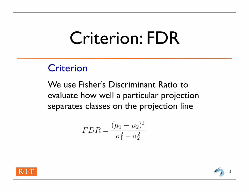
Criterion: FDR
Criterion
We use Fisher’s Discriminant Ratio to evaluate how well a particular projection separates classes on the projection line
5
FDR =(µ1 ! µ2)2
!21 + !2
2
FDR1 =|!|!
i=1
|!|!
j "=i
(µ1 ! µ2)2
!21 + !2
2
3

FDR for LDA
6
y =wTx
||w||
µ̃i = wTµi
(µ̃1 ! µ̃2)2 = wT (µ1 ! µ2)(µ1 ! µ2)
Tw = wTSbw
!̃2i = E[(y!µi)
2] = E[wT (x!µ)(x!µi)Tw)] = wT!iw
!21 + !2
2 " wTSww
FDR(w) =wTSbw
wTSww
5
y =wTx
||w||
µ̃i = wTµi
(µ̃1 ! µ̃2)2 = wT (µ1 ! µ2)(µ1 ! µ2)
Tw = wTSbw
!̃2i = E[(y!µ̃i)
2] = E[wT (x!µ)(x!µi)Tw)] = wT!iw
!21 + !2
2 " wTSww
FDR(w) =wTSbw
wTSww
5
y =wTx
||w||
µ̃i = wTµi
(µ̃1 ! µ̃2)2 = wT (µ1 ! µ2)(µ1 ! µ2)
Tw = wTSbw
!̃2i = E[(y!µ̃i)
2] = E[wT (x!µ)(x!µi)Tw)] = wT!iw
!21 + !2
2 " wTSww
FDR(w) =wTSbw
wTSww
5
Between class scatter
Covariance matrix
Within class scatter
Recall:
Modified Criterion for LDA:(Raleigh Quotient)
y =wTx
||w||
µ̃i = wTµi
(µ̃1 ! µ̃2)2 = wT (µ1 ! µ2)(µ1 ! µ2)
Tw " wTSbw
!̃2i = E[(y!µ̃i)
2] = E[wT (x!µ)(x!µi)Tw)] = wT!iw
!21 + !2
2 " wTSww
FDR(w) =wTSbw
wTSww
5
y =wTx
||w||
µ̃i = wTµi
(µ̃1 ! µ̃2)2 = wT (µ1 ! µ2)(µ1 ! µ2)
Tw " wTSbw
!̃2i = E[(y!µ̃i)
2] = E[wT (x!µ)(x!µi)Tw)] = wT!iw
!̃12 + !̃2
2 " wTSww
FDR(w) =wTSbw
wTSww
5
FDR =(µ̃1 ! µ̃2)2
!̃12 + !̃2
2
Sbw = "Sww
S!1w Sb
w = S1w!1(µ1 ! µ2)
6

Finding the Optimal Projection Direction w
Our Goal: Find w maximizing FDR(w)
• achieved if w chosen such that:
• where lambda is the largest eigenvalue of
• For two classes, to get the direction of w, use:
• This is the optimal reduction of m features to one for class separation
7
y =wTx
||w||
µ̃i = wTµi
(µ̃1 ! µ̃2)2 = wT (µ1 ! µ2)(µ1 ! µ2)
Tw = wTSbw
!̃2i = E[(y!µ̃i)
2] = E[wT (x!µ)(x!µi)Tw)] = wT!iw
!21 + !2
2 " wTSww
FDR(w) =wTSbw
wTSww
5
Sbw = !Sww
6
Sbw = !Sww
S!1w Sb
6
FDR =(µ̃1 ! µ̃2)2
!̃12 + !̃2
2
Sbw = "Sww
S!1w Sb
w = S!1w (µ1 ! µ2)
6

A Classifier for ‘Free’
Linear classifier also defined by LDA:
w0 not defined directly by LDA; for Gaussians with identical covariances optimal classifier is:
8
FDR =(µ̃1 ! µ̃2)2
!̃12 + !̃2
2
Sbw = "Sww
S!1w Sb
w = S!1w (µ1 ! µ2)
g(x) = (µ1 ! µ2)TS!1
w
!
"x! 1
2(µ1 + µ2)
#
$! lnP (#2)
P (#1
6
g(x) = (µ1 ! µ2)TS!1
w x + w0
7
(class 1 if >= 0, class two if < 0)

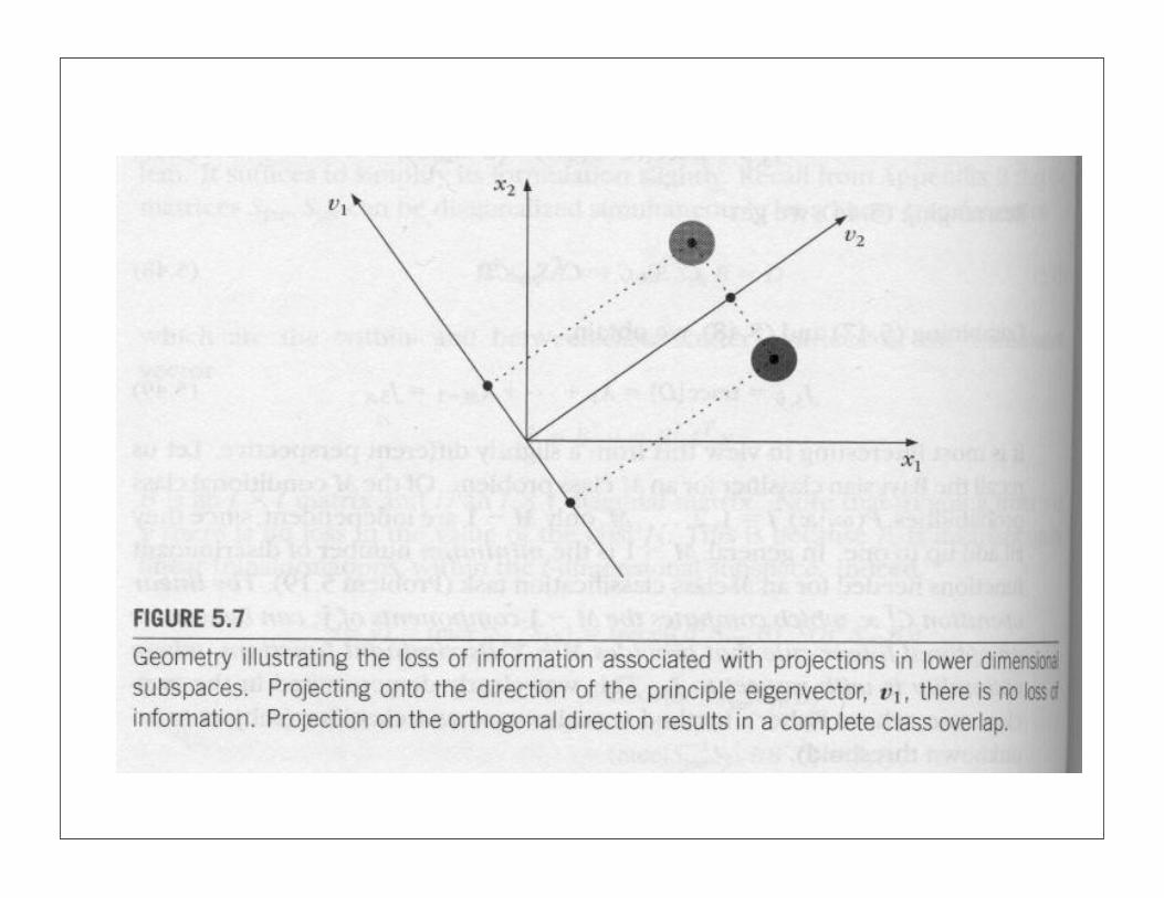
LDA, Cont’d
If original distributions multimodal and overlapping:
Classes for samples will overlap in the projection (little use)
Generalization for multiple classes is discussed further in the Theodoridis text.
10

Karhunen-Loève Transform (Principal Components Analysis - PCA)
Key Idea:
Model points in feature space by their deviation from the global mean in the primary directions of variation in feature space
• Defines a new, smaller feature space, often with more discriminating information
Directions of variation are computed from the global covariance matrix (unsupervised)
11

PCA Transform(Abridged)
1. Compute mean, covariance matrix for training set
• e.g. MATLAB: m = mean(Train); C = cov( Train.data );
2. Find the (unit-length) eigenvectors of the covariance matrix (see DHS Appendix A2.7) - complexity O(D3) for DxD matrix
• e.g. MATLAB: [ V, L ] = eig( C )
3. Sort eigenvectors by decreasing eigenvalue
4. Choose k eigenvectors with largest eigenvalues (principal components)
5. Return components as columns of a matrix, and associated eigenvalues (in a diagonal matrix) 12

Selection of Components
k Largest Eigenvalues
Correspond to eigenvectors in primary directions of variation within the data
• Large eigenvalues may be interpreted as the “inherent dimensionality” of ‘signal’ in the data
• Often only a small number of large eigenvalues
m - k Remaining Eigenvalues
Generally contain noise (random variation)13

Why PCA?Features are mutually uncorrelated (artifact of covariance matrix being real and symmetric)
The feature space reduction produced by a PCA with k components minimizes the mean-squared error between samples in the original space, and the newly transformed space, for any k-element transform matrix:
14
x = µ0 +d!
i=1aiei
x̂ = µ0 +k!
i=1aiei
Jk =n!
i=1||(µ0 +
k!
j=1aijei)! xi||2
8


The New Order (Feature Space)
Feature Space after PCA:
Becomes coefficients of the principal components (first, including all d eigenvectors):
To reduce feature space size, we limit the number of principle components to k:
16
x = µ0 +d!
i=1aiei
8
x = µ0 +d!
i=1aiei
x̂ = µ0 +k!
i=1aiei
8
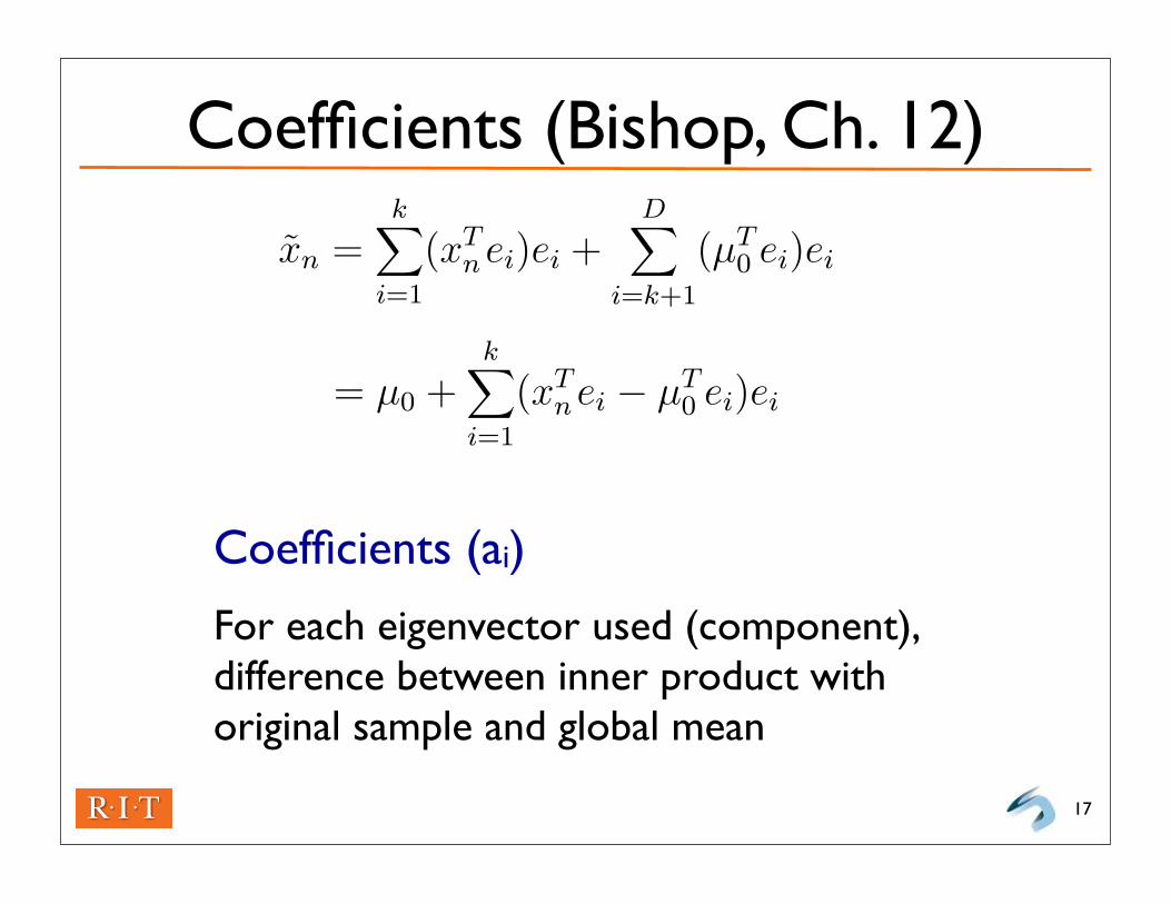
Coefficients (Bishop, Ch. 12)
Coefficients (ai)
For each eigenvector used (component), difference between inner product with original sample and global mean
17
PCA Revisited
x̃n =k!
i=1
(xTnei)ei +
D!
i=k+1
(µT0 ei)ei
= µ0 +k!
i=1
(xTnei ! µT
0 ei)ei
4

Example: MNIST (Bishop, Ch. 12)
18
M: # Principal Components Utilized(max. components = 784 (28x28))
Eigenvectors shown in yellowish-green: eigenvalues above images
Eigenvalue spectrum for digit data: