Information Sciences 279 (2014) 163–175

Contents lists available at ScienceDirect

Information Sciences

journal homepage: www.elsevier .com/locate / ins

Feature selection for Support Vector Machines via Mixed IntegerLinear Programming

http://dx.doi.org/10.1016/j.ins.2014.03.1100020-0255/� 2014 Elsevier Inc. All rights reserved.

⇑ Corresponding author. Tel.: +56 2 26181874.E-mail address: smaldonado@uandes.cl (S. Maldonado).

Sebastián Maldonado a,⇑, Juan Pérez a, Richard Weber b, Martine Labbé c

a Universidad de los Andes, Mons. Álvaro del Portillo 12455, Las Condes, Santiago, Chileb Department of Industrial Engineering, Universidad de Chile, República 701, Santiago, Chilec Computer Science Department, Université Libre de Bruxelles, Boulevard du Triomphe, B-1050 Brussels, Belgium

a r t i c l e i n f o

Article history:Received 4 August 2013Received in revised form 5 February 2014Accepted 26 March 2014Available online 2 April 2014

Keywords:Feature selectionSupport Vector MachineMixed Integer Linear Programming

a b s t r a c t

The performance of classification methods, such as Support Vector Machines, dependsheavily on the proper choice of the feature set used to construct the classifier. Featureselection is an NP-hard problem that has been studied extensively in the literature. Moststrategies propose the elimination of features independently of classifier construction byexploiting statistical properties of each of the variables, or via greedy search. All such strat-egies are heuristic by nature. In this work we propose two different Mixed Integer LinearProgramming formulations based on extensions of Support Vector Machines to overcomethese shortcomings. The proposed approaches perform variable selection simultaneouslywith classifier construction using optimization models. We ran experiments on real-worldbenchmark datasets, comparing our approaches with well-known feature selection tech-niques and obtained better predictions with consistently fewer relevant features.

� 2014 Elsevier Inc. All rights reserved.

1. Introduction

Support Vector Machines (SVMs) has been shown to be a very powerful machine learning method. For classification tasksand based on the structural risk minimization principle [18], this method attempts to find the separating hyperplane whichhas the largest distance from the nearest training data points of any class. SVM provides several advantages such as adequategeneralization to new objects, a flexible non-linear decision boundary, absence of local minima, and a representation thatdepends on only a few parameters [18,21].

Feature selection is one of the most important steps within classification. An appropriate selection of the most relevantfeatures reduces the risk of overfitting, thus improving model generalization by decreasing the model’s complexity [7]. Thisis particularly important in small-sized high-dimensional datasets, where the curse of dimensionality is present and a signif-icant gain in terms of performance can be achieved with a small subset of features [9,13]. Additionally, low-dimensionalrepresentation allows better interpretation of the resulting classifier. This is particularly important in applications in fieldssuch as business analytics, since many machine learning approaches are considered to be black boxes by practitioners whotherefore tend to be hesitant to use these techniques [6]. A better understanding of the process that generates the data byidentifying the most relevant features is also of crucial importance in life sciences, where we want to identify, for example,

164 S. Maldonado et al. / Information Sciences 279 (2014) 163–175

those genes that best explain the presence of a particular type of cancer, and therefore could improve cancer incidenceprediction.

Since the selection of the best feature subset is considered to be an NP-hard combinatorial problem, many heuristicapproaches for feature selection have been presented to date [7]. With the two Mixed Integer Linear Programs for simulta-neous feature selection and classification that we introduce in this paper we show that integer programming has become acompetitive approach using state-of-the-art hardware and solvers.

In particular, we propose two novel SVM-based formulations for embedded feature selection, which simultaneouslyselect relevant features during classifier construction by introducing indicator variables and constraining their selectionvia a budget constraint. The first approach studies an adaptation of the l1-SVM formulation [4], while the second oneextends the LP-SVM method presented in [22]. Our experiments show that the proposed methods are capable of select-ing a few relevant features in all datasets used, leading to highly accurate classifiers within reasonable computationaltime.

Section 2 of this paper introduces Support Vector Machines for binary classification, including recent developments forfeature selection using SVMs. The proposed feature selection approaches are presented in Section 3. Section 4 providesexperimental results using real-world datasets. A summary of this paper can be found in Section 5, where we provide itsmain conclusions and address future developments.

2. Prior work on support vector classification

The mathematical derivation of the standard l2-SVM formulation [18], the l1-SVM formulation [4], and the LP-SVMmethod [22] are described in this section. The latter two linear classification methods constitute the basis for our proposedfeature selection algorithms.

2.1. l2-Support Vector Machine

Considering training examples xi 2 Rn with their respective labels yi 2 f�1;þ1g; i ¼ 1; . . . ;m, SVM determines a hyper-plane f ðx;aÞ to separate the training examples optimally according to their labels, where a 2 K, is the set of possible modelparameters.

This optimal split is based on Statistical Learning Theory [18], which provides a general measure of complexity (the VCdimension), and estimates a bound for the expected risk RðaÞ as a function of the empirical risk RempðaÞ. According to thistheory, the following inequality holds with probability 1� g [22]:

RðaÞ 6 RempðaÞ þe2

1þffiffiffiffiffiffiffiffiffiffiffiffiffiffiffiffiffiffiffiffiffiffiffiffiffiffiffiffi1þ 4RempðaÞ

e

r !; ð1Þ

where e is a function of the VC dimension h (a measure of complexity defined by the largest number of points that canbe shattered by members of f ðx;aÞ), g, and the number of instances m (� ¼ 4ðhðlnð2m=hÞ þ 1Þ � ln gÞ=m). We observethat minimizing the expected risk is equivalent to simultaneously minimizing the two terms on the right-hand side ofEq. (1).

Considering a linear hyperplane of the form f ðxÞ ¼ w> � xþ b, the SVM hyperplane then minimizes the classificationerrors and at the same time maximizes the margin, which is computed as the sum of the distances to one of the closest posi-tive and one of the closest negative training examples, and is linked to Statistical Learning Theory since maximizing the mar-gin is similar to minimizing the VC dimension [22].

To maximize the margin, we need to classify the training vectors xi correctly into the two different classes, using thesmallest norm of coefficients w 2 Rn [18]. The primal SVM formulation balances the minimization of wk k2

2 (structural risk)and of the misclassification errors (empirical risk) by introducing an additional set of slack variables ni; i ¼ 1; . . . ;m and apenalty parameter, C, that controls the trade-off between both objectives:

minw;b;n

12 wk k2

2 þ CXm

i¼1

ni

s:t: yi � ðw> � xi þ bÞP 1� ni; i ¼ 1; . . . ;m;

ni P 0; i ¼ 1; . . . ;m:

ð2Þ

2.2. l1-Support Vector Machine

Bradley and Mangasarian [4] proposed a variation of SVM, reducing the model’s complexity by using the l1-norm (alsoknown as LASSO penalty) instead of the Euclidean norm. This norm provides a strategy for suppressing redundant and/orirrelevant features automatically, i.e. components of the vector w, while converting the quadratic programming problemstudied by l2-SVM (Formulation (2)) into a linear one. This formulation follows:

S. Maldonado et al. / Information Sciences 279 (2014) 163–175 165

minw;b;n

wk k1 þ CXm

i¼1

ni

s:t: yi � ðw> � xi þ bÞP 1� ni; i ¼ 1; . . . ;m;

ni P 0; i ¼ 1; . . . ;m:

ð3Þ

Formulation (3) can be cast into a linear programming model, tackling the sum of absolute values from vector w with thefollowing formulation (l1-SVM):

minw;v;b;n

Xn

j¼1

v j þ CXm

i¼1

ni

s:t: yi � ðw> � xi þ bÞP 1� ni; i ¼ 1; . . . ;m;�v j 6 wj 6 v j; j ¼ 1; . . . ;n;

ni P 0; i ¼ 1; . . . ;m;

v j P 0; j ¼ 1; . . . ;n:

ð4Þ

2.3. Linear programming Support Vector Machine

Another strategy based on SVM was proposed by [22], where the bound of the VC dimension is loosened properly usingthe l1-norm, resulting in a linear programming formulation that directly controls the margin maximization by considering amargin variable, r. The authors define a set of mD-margin separating hyperplanes of the form f ðxÞ ¼ w> � xþ b as follows:

y ¼þ1 w>xþ b P D

�1 w>xþ b 6 �D

�; ð5Þ

with D P 0, and determining a bound for the VC dimension, h, based on this family of hyperplanes, as shown in the followingtheorem.

Theorem 2.1 [22]. Given a set of training instances xi 2 Rn and their respective labels yi 2 �1;þ1f g; i ¼ 1; . . . ;m, and a set ofmD-margin separating hyperplanes, then there exists a constant 0 < c <1 such that:

h 6 minc2R2 wk k2

b

D2

" #; n

!þ 1 ð6Þ

holds true, where k � kb is any vector norm.The authors studied b ¼ 1 and c ¼ 1. Based on this choice, the LP-SVM (soft-margin) formulation follows:

minw;r;b;n

� r þ CXm

i¼1

ni

s:t: yi � ðw> � xi þ bÞP r � ni; i ¼ 1; . . . ;m;

�1 6 wj 6 1; j ¼ 1; . . . ;n:ni P 0; i ¼ 1; . . . ;m:

r P 0;

ð7Þ

where as in previously presented models, C is a positive parameter that can be calibrated using cross-validation. The decisionfunction of LP-SVM is also similar to standard SVM. The variable r is maximized while assuring - in the case of separabletraining examples – that each observation is on the correct side of the hyperplane, and at a distance at least r from it. Forthe non-separable case, the empirical risk is minimized simultaneously by penalizing a set of slack variables, similarly tostandard SVM. Notice that the second constraint is related to the l1-norm of the weight vector.

The approach was tested on simulated and real datasets in Zhou et al. [22], leading to at least one order of magnitudeimprovement in training speed, making it particularly suitable for complex machine learning tasks, such as large scale prob-lems or feature selection.

2.4. Related work on feature selection for SVMs

Guyon et al. [7] identified three main categories of methods for feature selection: filter, wrapper, and embedded methods.Filter methods eliminate poorly informative features based on their statistical properties prior to applying any classificationalgorithm. A commonly used filter method is the Fisher Criterion Score (F), which computes each feature’s importance inde-pendently of the other features by comparing that feature’s correlation to the output labels [7]:

166 S. Maldonado et al. / Information Sciences 279 (2014) 163–175

FðjÞ ¼lþj � l�j

ðrþj Þ2 þ ðr�j Þ

2

���������� ð8Þ

where lþj (l�j ) represents the mean of the j-th feature for the positive (negative) class and rþj (r�j ) is the respective standarddeviation.

Wrapper methods interact with the respective classification technique and explore the entire set of variables to identifygood feature subsets according to their predictive power, which is computationally demanding, but often provides betterresults than filter methods. Common wrapper strategies are Sequential Forward Selection (SFS) and Sequential BackwardElimination (SBE) [11]. A combination of filter methods and wrappers that focuses however, on fuzziness in the analyzeddata has been presented by [17].

Techniques from the third category (embedded methods) select features and simultaneously construct the respective clas-sifier, which can be seen as a search in the combined space of feature subsets and hypotheses. Unlike wrapper methods,which depend on a given but separate classification algorithm, in this category it is just one technique that performs bothtasks, feature selection as well as classifier construction. In general, embedded methods have the advantage of beingcomputationally less intensive than wrapper methods [7].

Recursive Feature Elimination (RFE-SVM) [8] is a popular embedded technique which tries to find a subset of size s amongn variables (s < n), eliminating those whose removal leads to the largest margin of class separation. This can be achievedusing a linear approach, based on the value of the weight vector w. While one could choose a single variable to removeat each iteration, this would be inefficient in many high-dimensional applications (e.g. microarray data). Such datasetsare often characterized by thousands of features, and their respective authors usually remove half of the remaining variablesin each step [8].

Embedded feature selection can also be seen as an optimization problem. This is generally done by forcing feature selec-tion into the model, considering a sparsity term in the objective function. One example is the minimization of the ‘‘zero-norm’’: XðwÞ ¼ kwk0 ¼ j i : wi – 0f gj.

Weston et al. [20] proposed an approach for ‘‘zero-norm’’ minimization (l0-SVM) by iteratively scaling the variables, mul-tiplying them by the absolute value of the weight vector w, which is obtained from the SVM formulation, until convergenceis reached. Variables can be ranked by removing those features whose weights become zero during the iterative algorithmand computing the order of removal.

A mixed-integer program (MIP) has been proposed to select features iteratively for a non-linear SVM classifier [14]. In thisapproach any suitable kernel function can be used and the MIP is solved efficiently by alternating between a linear programwhich determines the continuous variable values of the classifier and successive updates of the binary variables indicatingpresence or absence of the respective features.

In an early work [10] titled ‘‘Feature Selection for Multiclass Discrimination via Mixed-Integer Linear Programming’’, aMILP for feature selection based on the assumption of feature independence had been introduced. Later, an alternativemixed-integer programming approach was proposed for simultaneous feature selection and multi-class classification [5].This method modifies the l1 multi-class SVM formulation to include costs on features, which has also been proposed for deci-sion trees by Turney [16]. A biobjective optimization scheme is considered to maximize fit and minimize the total featurecosts simultaneously, leading to an approximation of the set of Pareto-optimal classifiers.

Our work differs from previous ones in which a multi-objective approach balances both objectives requiring additionalinformation regarding their trade-off. Instead, we propose an additional budget constraint providing direct controlover the number of selected features and solving a Mixed Integer Linear Program with a single objective, as will be shownnext.

3. Proposed SVM-based MILP formulations

In each one of the following two subsections we propose a model based on previously introduced SVM formulations,namely l1-SVM and LP-SVM. In both cases, the main idea is to perform embedded feature selection by using a binary variablelinked to each attribute, and to restrict the number of attributes used in the respective classifier via a budget constraint.We assume a cost vector, c 2 Rn, where cj is the cost of acquiring attribute j; j ¼ 1; . . . ;n. If no such cost information isprovided or equal cost among attributes is desired, all parameters cj can be set to 1. Both proposed models use a fixed‘‘budget’’ B to limit the number of selected features. The difference between them is the respective norm used for theSVM formulation.

3.1. MILP Formulation based on l1-SVM: MILP1

The following model emulates the l1-SVM formulation described in Section 2.2, where the l1-norm of w, represented byPnj¼1v j, is minimized simultaneously with the minimization of the sum of the classification errors (

Pmi¼1ni), which requires

the additional parameter C.In our proposed MILP1 formulation we select features using a budget constraint instead of minimizing the l1-norm of w,

and force each weight wj to belong to a given interval ½lj;uj�, if the attribute is selected (i.e. if v j ¼ 1). In this way we link the

S. Maldonado et al. / Information Sciences 279 (2014) 163–175 167

weight vector w and the binary variables v in the formulation. Additionally, we avoid the inclusion of a trade-off parameter Csince the shrinkage is now performed by the second and third constraints, instead of minimizing the l1-norm in the objectivefunction.

minw;v;b;n

Xm

i¼1

ni

s:t: yi � ðw> � xi þ bÞP 1� ni; i ¼ 1; . . . ;m;

ljv j 6 wj 6 ujv j; j ¼ 1; . . . ;n:Xn

j¼1

cjv j 6 B:

v j 2 f0;1g; j ¼ 1; . . . ;n:

ni P 0; i ¼ 1; . . . ;m:

ð9Þ

The previous formulation presents interesting properties. For instance, we define a budget B explicitly, which represents thenumber of features in the classifier when all cj are equal to 1. Additionally, the budget constraint allows incorporating acqui-sition costs directly into the formulation, encouraging a cheaper solution with an adequate level of accuracy.

The formulation, however, has a higher computational cost than linear or quadratic programming approaches. An impor-tant issue is the appropriate choice of the lower and upper bounds for the components of vector w, i.e. l and u. Of course, wecan always choose lower and upper bounds with arbitrarily high values (positive or negative). However, the genericapproach for solving MILP formulations like (9) consists of a Branch-and-Cut method whose efficiency depends heavilyon the tightness of the model’s LP-relaxation, i.e. how close the optimal values of the MILP and its LP-relaxation are, whichin turn strongly depends on the tightness of the lower and upper bounds. In Section 4.4 we study the influence of theseparameters.

3.2. MILP formulation based on LP-SVM: MILP2

The second formulation we propose extends the LP-SVM model to Mixed Integer Linear Programming. Similar to MILP1,MILP2 includes binary variables to activate the usage of the different attributes, limiting the number of selected variables inthe classifier via a budget constraint. The main difference between the two models is that the weight vectors are nowbounded by the interval ½�1;1�, only if a particular variable is selected (i.e. if v j ¼ 1), instead of a predefined intervallj;uj� �

. These constraints are directly linked to the l1-norm of the weight vector used for the bound of the VC dimensiondescribed by Zhou et al. [22]. The second difference is that, for MILP2, a margin variable r is now maximized, in the attemptto find the mD-margin separating hyperplane with maximum margin, instead of using the classical constraint based on theconstruction of the canonical hyperplanes. The proposed formulation follows:

minw;r;b;n;v

� r þ CXm

i¼1

ni

s:t: yi � ðw> � xi þ bÞP r � ni; i ¼ 1; . . . ;m;

�v j 6 wj 6 v j; j ¼ 1; . . . ;n:Xn

j¼1

cjv j 6 B;

ni P 0; i ¼ 1; . . . ;m:

v j 2 f0;1g; j ¼ 1; . . . ;n:

ð10Þ

Additionally, we identified the following two practical pitfalls in the LP-SVM formulation presented in Section 2.3, whichit is necessary for us to address in our proposed formulation, given the higher complexity of our approach.

� One possible solution of the optimization problem is that all variables become zero. In that extreme case, all object labelswill be predicted as zero, resulting in an accuracy of 0%. High values of C in noisy data may trigger that issue. This can beavoided by using a lower bound rlo > 0 for variable r. In our experiments we use the value rlo ¼ 0:001.� Another issue is that the variables r and ni may grow unboundedly, given their relationship in the objective function.

When this happens, results are very inaccurate. Setting an upper bound on variable r (rup) avoids this effect, also control-ling the growth of the variables ni. Different values for rup are studied using line search; see Section 4.4.

To address both issues, we included an additional constraint to bound the margin variable r between both lower andupper values.

168 S. Maldonado et al. / Information Sciences 279 (2014) 163–175

minw;r;b;n;v

� r þ CXm

i¼1

ni

s:t: yi � ðw> � xi þ bÞP r � ni; i ¼ 1; . . . ;m;

�v j 6 wj 6 v j; j ¼ 1; . . . ;n:Xn

j¼1

cjv j 6 B;

ni P 0; i ¼ 1; . . . ;m:

v j 2 f0;1g; j ¼ 1; . . . ;n:

rlo 6 r 6 rup;

ð11Þ

This formulation does not require the determination of lower and upper bounds (i.e. lj; uj) for the variables wj, which inmodel (11) can take values only from the interval [�1,1]. The desired flexibility for variables wj is achieved indirectly byusing the non-negative variable r which explicitly considers the structural risk minimization principle. As a consequence,model (11) requires the additional regularization parameter C. The final constraint in model (11) prohibits r becoming zeroor diverging.

4. Experimental results

In this section we apply the classification models l2-Support Vector Machines (Formulation (2)) and LP-Support VectorMachines (Formulation (7)) as well as the feature selection approaches l1-Support Vector Machines (Formulation (4)), l0-Sup-port Vector Machines, and the two benchmark techniques for feature selection (Fischer + SVM and RFE-SVM) to various data-sets, in comparison with the newly proposed formulations for simultaneous feature selection and classification via Mixed-Integer Linear Programming (MILP1: Model (9) and MILP2: Model (11)).

These datasets are presented in Section 4.1. Subsequently, we describe our model selection procedure. Section 4.3 pre-sents the results we obtained. The influence of the different parameters on robustness and stability are studied in Section 4.4.Finally, we analyze running times for all methods used in our experiments in Section 4.5.

4.1. Datasets

We applied the proposed approaches on six well-known datasets from the UCI Repository [3]. These datasets have alreadybeen used for benchmark studies regarding the performance of Support Vector Machines (see e.g. [1,15]).

� Australian Credit (AUS): This dataset contains 690 granted loans; 383 good repayers and 307 bad repayers,described by 14 variables.

� Wisconsin Breast Cancer (WBC): This dataset contains 569 observations of tissues (212 malignant and 357 benigntumors) described by 30 continuous features.

� Pima Indians Diabetes (PIMA): The Pima Indians Diabetes dataset presents 8 features and 768 examples (500 testednegative for diabetes and 268 tested positive).

� German Credit (GC): This dataset presents 1000 granted loans; 700 good repayers and 300 bad repayers, describedby 24 attributes.

� Ionosphere (IONO): This dataset presents 351 data points; 225 labeled as good radar returns (evidence of some typeof structure in the Ionosphere) and 126 labeled as bad radar returns (no evidence of structure), described by 34attributes.

� Splice: This dataset contains 1000 randomly selected examples (from the complete set of 3190 splice junctions),where 517 are labeled as IE borders and 483 as EI borders, described by 60 categorical variables (the gene sequence).Given a DNA sequence, the problem posed in this dataset is to recognize the boundaries between exons and introns(the parts of the sequence retained after splicing and the parts that are spliced out, respectively).

Additionally, we analyzed a microarray dataset in order to study the performance of the proposed methods under con-ditions of high dimensionality with a small number of examples.

� Colorectal Microarray (CoMA) [2]: This dataset contains the expression of the 2000 genes with highest minimal intensityacross 62 samples (40 tumor and 22 normal).

4.2. Model selection

The following model selection procedure was performed: training and test subsets were constructed using 10-fold cross-validation and the average AUC (Area Under Curve) was computed. For the microarray dataset we followed the procedurepresented in [19]: training and test subsets were obtained using a leave-one-out procedure. Feature selection and classifi-

S. Maldonado et al. / Information Sciences 279 (2014) 163–175 169

cation were then performed on the training set, and the classification performance was finally computed from test results.We performed a grid search to study the influence of parameter C for soft-margin models, and other model-specific param-eters; (see Section 4.4).

The intervals were further divided into homogenous values in order to characterize the relevant area for this parameter(where maximum predictive performance is reached). The parameter B for the budget constraint was varied along all pos-sible numbers of attributes for the first six datasets. For the Colorectal Microarray dataset the following budget values werestudied:

B 2 f10;20;50;100;250;500;1000;2000g.All values of the feature cost vector c were set to 1 since we do not have specific cost information in our experiments. The

optimization was performed using LIBSVM in the case of l2-Support Vector Machines, LINPROG solver for Matlab 7.8 in thecase of l1-Support Vector Machines (Formulation (4)), and CPLEX 9.1 solver for the LP-Support Vector Machines, MILP1, andMILP2 approaches. The experiments were performed in a Lenovo x220t with 16 GB RAM, 750 GB SSD, a i7-2620M processorwith 2.70 GHz, and Microsoft Windows 8.1 Operating System (64-bit).

4.3. Results

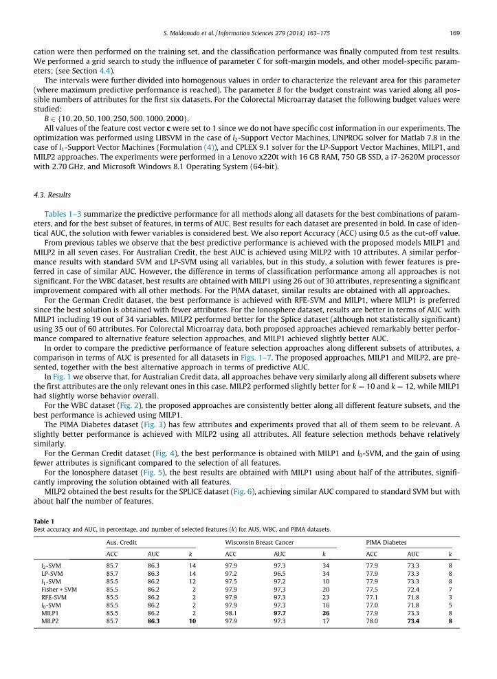
Tables 1–3 summarize the predictive performance for all methods along all datasets for the best combinations of param-eters, and for the best subset of features, in terms of AUC. Best results for each dataset are presented in bold. In case of iden-tical AUC, the solution with fewer variables is considered best. We also report Accuracy (ACC) using 0.5 as the cut-off value.

From previous tables we observe that the best predictive performance is achieved with the proposed models MILP1 andMILP2 in all seven cases. For Australian Credit, the best AUC is achieved using MILP2 with 10 attributes. A similar perfor-mance results with standard SVM and LP-SVM using all variables, but in this study, a solution with fewer features is pre-ferred in case of similar AUC. However, the difference in terms of classification performance among all approaches is notsignificant. For the WBC dataset, best results are obtained with MILP1 using 26 out of 30 attributes, representing a significantimprovement compared with all other methods. For the PIMA dataset, similar results are obtained with all approaches.

For the German Credit dataset, the best performance is achieved with RFE-SVM and MILP1, where MILP1 is preferredsince the best solution is obtained with fewer attributes. For the Ionosphere dataset, results are better in terms of AUC withMILP1 including 19 out of 34 variables. MILP2 performed better for the Splice dataset (although not statistically significant)using 35 out of 60 attributes. For Colorectal Microarray data, both proposed approaches achieved remarkably better perfor-mance compared to alternative feature selection approaches, and MILP1 achieved slightly better AUC.

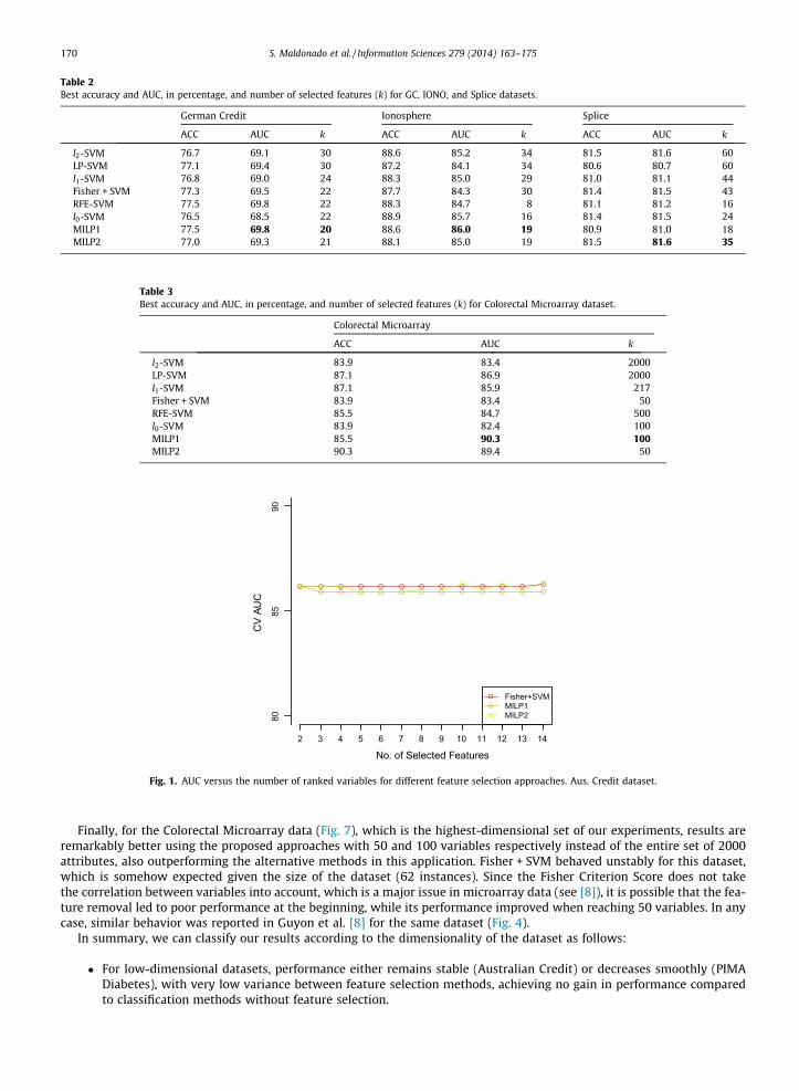
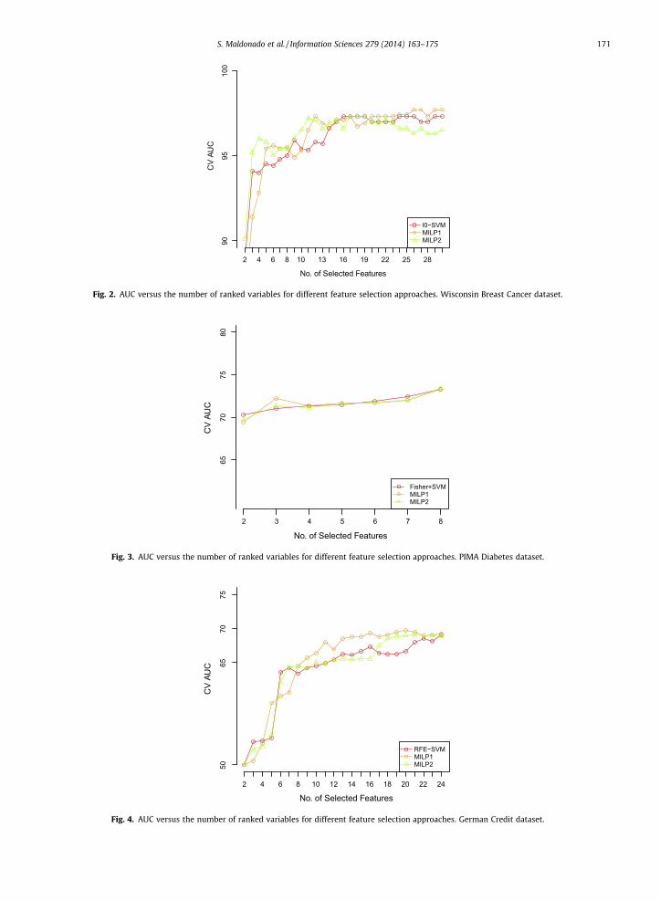
In order to compare the predictive performance of feature selection approaches along different subsets of attributes, acomparison in terms of AUC is presented for all datasets in Figs. 1–7. The proposed approaches, MILP1 and MILP2, are pre-sented, together with the best alternative approach in terms of predictive AUC.

In Fig. 1 we observe that, for Australian Credit data, all approaches behave very similarly along all different subsets wherethe first attributes are the only relevant ones in this case. MILP2 performed slightly better for k ¼ 10 and k ¼ 12, while MILP1had slightly worse behavior overall.

For the WBC dataset (Fig. 2), the proposed approaches are consistently better along all different feature subsets, and thebest performance is achieved using MILP1.

The PIMA Diabetes dataset (Fig. 3) has few attributes and experiments proved that all of them seem to be relevant. Aslightly better performance is achieved with MILP2 using all attributes. All feature selection methods behave relativelysimilarly.

For the German Credit dataset (Fig. 4), the best performance is obtained with MILP1 and l0-SVM, and the gain of usingfewer attributes is significant compared to the selection of all features.

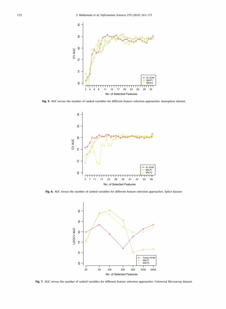
For the Ionosphere dataset (Fig. 5), the best results are obtained with MILP1 using about half of the attributes, signifi-cantly improving the solution obtained with all features.

MILP2 obtained the best results for the SPLICE dataset (Fig. 6), achieving similar AUC compared to standard SVM but withabout half the number of features.

Table 1Best accuracy and AUC, in percentage, and number of selected features (k) for AUS, WBC, and PIMA datasets.

Aus. Credit Wisconsin Breast Cancer PIMA Diabetes

ACC AUC k ACC AUC k ACC AUC k

l2-SVM 85.7 86.3 14 97.9 97.3 34 77.9 73.3 8LP-SVM 85.7 86.3 14 97.2 96.5 34 77.9 73.3 8l1-SVM 85.5 86.2 12 97.5 97.2 10 77.9 73.3 8Fisher + SVM 85.5 86.2 2 97.9 97.3 20 77.5 72.4 7RFE-SVM 85.5 86.2 2 97.9 97.3 23 77.1 71.8 3l0-SVM 85.5 86.2 2 97.9 97.3 16 77.0 71.8 5MILP1 85.5 86.2 2 98.1 97.7 26 77.9 73.3 8MILP2 85.7 86.3 10 97.9 97.3 17 78.0 73.4 8

Table 2Best accuracy and AUC, in percentage, and number of selected features (k) for GC, IONO, and Splice datasets.

German Credit Ionosphere Splice

ACC AUC k ACC AUC k ACC AUC k

l2-SVM 76.7 69.1 30 88.6 85.2 34 81.5 81.6 60LP-SVM 77.1 69.4 30 87.2 84.1 34 80.6 80.7 60l1-SVM 76.8 69.0 24 88.3 85.0 29 81.0 81.1 44Fisher + SVM 77.3 69.5 22 87.7 84.3 30 81.4 81.5 43RFE-SVM 77.5 69.8 22 88.3 84.7 8 81.1 81.2 16l0-SVM 76.5 68.5 22 88.9 85.7 16 81.4 81.5 24MILP1 77.5 69.8 20 88.6 86.0 19 80.9 81.0 18MILP2 77.0 69.3 21 88.1 85.0 19 81.5 81.6 35

Table 3Best accuracy and AUC, in percentage, and number of selected features (k) for Colorectal Microarray dataset.

Colorectal Microarray

ACC AUC k

l2-SVM 83.9 83.4 2000LP-SVM 87.1 86.9 2000l1-SVM 87.1 85.9 217Fisher + SVM 83.9 83.4 50RFE-SVM 85.5 84.7 500l0-SVM 83.9 82.4 100MILP1 85.5 90.3 100MILP2 90.3 89.4 50

No. of Selected Features

CV

AUC

Fisher+SVMMILP1MILP280

8590

2 3 4 5 6 7 8 9 10 11 12 13 14

Fig. 1. AUC versus the number of ranked variables for different feature selection approaches. Aus. Credit dataset.

170 S. Maldonado et al. / Information Sciences 279 (2014) 163–175

Finally, for the Colorectal Microarray data (Fig. 7), which is the highest-dimensional set of our experiments, results areremarkably better using the proposed approaches with 50 and 100 variables respectively instead of the entire set of 2000attributes, also outperforming the alternative methods in this application. Fisher + SVM behaved unstably for this dataset,which is somehow expected given the size of the dataset (62 instances). Since the Fisher Criterion Score does not takethe correlation between variables into account, which is a major issue in microarray data (see [8]), it is possible that the fea-ture removal led to poor performance at the beginning, while its performance improved when reaching 50 variables. In anycase, similar behavior was reported in Guyon et al. [8] for the same dataset (Fig. 4).

In summary, we can classify our results according to the dimensionality of the dataset as follows:

� For low-dimensional datasets, performance either remains stable (Australian Credit) or decreases smoothly (PIMADiabetes), with very low variance between feature selection methods, achieving no gain in performance comparedto classification methods without feature selection.

No. of Selected Features

CV

AUC

l0−SVMMILP1MILP290

9510

0

2 4 6 8 10 13 16 19 22 25 28

Fig. 2. AUC versus the number of ranked variables for different feature selection approaches. Wisconsin Breast Cancer dataset.

No. of Selected Features

CV

AUC

Fisher+SVMMILP1MILP2

6570

7580

2 3 4 5 6 7 8

Fig. 3. AUC versus the number of ranked variables for different feature selection approaches. PIMA Diabetes dataset.

No. of Selected Features

CV

AUC

RFE−SVMMILP1MILP250

6570

75

2 4 6 8 10 12 14 16 18 20 22 24

Fig. 4. AUC versus the number of ranked variables for different feature selection approaches. German Credit dataset.

S. Maldonado et al. / Information Sciences 279 (2014) 163–175 171

No. of Selected Features

CV

AUC

l0−SVMMILP1MILP265

7075

8085

90

2 4 6 8 11 14 17 20 23 26 29 32

Fig. 5. AUC versus the number of ranked variables for different feature selection approaches. Ionosphere dataset.

No. of Selected Features

CV

AUC

l0−SVMMILP1MILP26570

7580

8590

3 7 11 17 23 29 35 41 47 53 59

Fig. 6. AUC versus the number of ranked variables for different feature selection approaches. Splice dataset.

No. of Selected Features

LOO

CV

AUC

Fisher+SVMMILP1MILP265

7075

8085

90

20 50 100 250 500 1000 2000

Fig. 7. AUC versus the number of ranked variables for different feature selection approaches. Colorectal Microarray dataset.

172 S. Maldonado et al. / Information Sciences 279 (2014) 163–175

S. Maldonado et al. / Information Sciences 279 (2014) 163–175 173

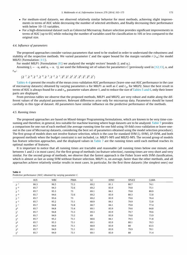
� For medium-sized datasets, we observed relatively similar behavior for most methods, achieving slight improve-ments in terms of AUC while decreasing the number of selected attributes, and finally decreasing their performancewith below 10–15 variables.

� For a high-dimensional dataset such as Colorectal Microarray, feature selection provides significant improvements interms of AUC (up to 6%) while reducing the number of variables used for classification to 10% or less compared to theoriginal size.

4.4. Influence of parameters

The proposed approaches consider various parameters that need to be studied in order to understand the robustness andstability of the respective methods. We varied parameter C and the upper bound for the margin variable r (rup) for modelMILP2 (Formulation (11)).

For model MILP1 (Formulation (9)) we analyzed the weight vectors’ bounds (lj and uj).Assuming lj ¼ �uj and uj ¼ u; 8j, we used the following set of values for parameters C (previously used in [12,13], u, and

rup:

Table 4Predicti

2�7

2�6

2�5

2�4

2�3

2�2

2�1

20

21

22

23

24

25

26

27

f2�7;2�6;2�5;2�4;2�3;2�2;2�1;20;21;22;23;24;25;26;27g

Tables 4–6 present the results of the mean cross-validation AUC performance (leave-one-out AUC performance in the caseof microarray datasets) obtained by varying parameters u for MILP1 as well as C and rup for MILP2. Since the best result interms of AUC is always found for u and rup parameter values above 1, and to reduce the size of Tables 5 and 6, only their lowerparts are displayed.

From previous tables we observe that the proposed methods, MILP1 and MILP2, are very robust and stable along the dif-ferent values of the analyzed parameters. Relevant differences arise only for microarray data. Parameters should be tunedcarefully in this type of dataset. All parameters have similar influence on the predictive performance of the methods.

4.5. Running times

The proposed approaches are based on Mixed-Integer Programming formulations, which are known to be very time-con-suming and therefore, in general, less suitable for machine learning where huge datasets are to be analyzed. Table 7 providesa comparison for one run of each method (the average running time for one fold using 10-fold cross-validation or leave-one-out in the case of Microarray datasets, considering the best set of parameters obtained using the model selection procedure).The first group of models does not involve feature selection, which is the case for standard SVM (l2-SVM), LP-SVM, and bothproposed methods when the budget constraint is not included, i.e. MILP1-NFS and MILP2-NFS. The second group of modelshas feature selection approaches, and the displayed values in Table 7 are the running times until each method reaches itsoptimal number of features.

It is important to notice that all running times are tractable and reasonable (all running times below one minute, andbetween 1 and 2 s in most cases). For the first group of methods (no feature selection), running times are very short and verysimilar. For the second group of methods, we observe that the fastest approach is the Fisher Score with SVM classification,which is almost as fast as using SVM without feature selection. MILP1 is, on average, faster than the other methods, and allapproaches achieve relatively similar results in most cases. In particular, for the first three datasets (the simplest ones) our

ve performance (AUC) obtained by varying parameter C.

AUS WBC PIMA GC IONO SPLICE CoMA

86.3 96.5 73.3 69.2 81.1 80.7 74.1

85.7 94.3 72.6 69.2 83.9 79.8 75.1

85.7 95.3 73 69.1 84.1 79.8 80.9

85.7 94.6 72.6 69.2 83.9 80.3 72.8

85.7 95.6 73 69.2 83.9 79.6 76.4

85.7 95.2 73.1 68.9 84.1 79.9 72.8

85.7 94.8 72.8 68.7 84.1 79.8 77.4

85.7 94.8 73.4 69.1 83.9 79.6 64.8

85.7 94.8 73.3 69.3 83.9 79.7 70.6

85.7 94.9 73.2 69 83.9 79.8 73.9

85.7 95.2 73.1 68.6 84.1 79.5 71.8

85.7 95.3 73.1 69.1 83.9 80.1 70.3

85.7 94.9 73.1 68.9 83.9 80 63.5

85.7 94.9 73.1 69.1 83.9 79.9 70.1

85.7 94.9 73.1 69.1 83.9 80 71.4

Table 5Predictive performance (AUC) obtained by varying parameter u.

AUS WBC PIMA GC IONO SPLICE CoMA

20 85.9 95.4 65.9 69.2 81.3 80.3 82.6

21 85.7 97.7 72.4 69.1 82.5 79.8 85.7

22 85.7 96.7 73.3 69.1 83.5 79.8 76.1

23 85.7 96.6 73.3 69.1 84.2 79.8 70.6

24 85.7 95.9 73.3 69.1 84.3 79.8 67.3

25 85.7 95.6 73.3 69.1 83.9 79.8 62.3

26 85.7 95.1 73.3 69.1 83.9 79.8 70.3

27 85.7 94.5 73.3 69.1 83.9 79.8 68.3

Table 6Predictive performance (AUC) obtained by varying parameter rup .

AUS WBC PIMA GC IONO SPLICE CoMA

20 85.9 96.5 73.3 68.9 83.9 80.3 76.4

21 86.3 96.5 73.3 68.9 83.9 80.7 81.1

22 86.3 96.5 73.3 68.9 83.9 80.7 76.4

23 86.3 96.5 73.3 68.9 83.9 80.7 82.2

24 86.3 96.5 73.3 68.9 83.9 80.7 79.7

25 86.3 96.5 73.3 68.9 83.9 80.7 82.2

26 86.3 96.5 73.3 68.9 83.9 80.7 86.9

27 86.3 96.5 73.3 68.9 83.9 80.7 86.9

Table 7Average running times, in seconds, for all datasets.

AUS WBC PIMA GC IONO SPLICE CoMA

l2-SVM 0.5 0.2 0.3 0.7 0.2 1.5 0.2LP-SVM 0.2 0.1 0.1 0.3 0.1 0.4 0.4MILP1-NFS 0.2 0.2 0.2 0.4 0.2 0.7 0.4MILP2-NFS 0.2 0.3 0.2 0.4 0.2 1.4 0.6Fisher + SVM 0.5 0.2 0.4 0.7 0.2 1.5 0.2l1-SVM 0.4 0.4 0.3 0.4 0.3 4.8 0.6RFE-SVM 0.8 0.4 0.6 0.7 0.6 2.3 1.7l0-SVM 0.8 0.5 1.3 1.7 0.4 2.4 1.8MILP1-FS 0.2 0.2 0.2 0.3 0.2 1.7 2.2MILP2-FS 0.3 0.2 0.3 0.9 2.3 51.6 3.2

174 S. Maldonado et al. / Information Sciences 279 (2014) 163–175

approaches are faster than the alternative feature selection methods. MILP2, however, presents significantly higher valuesfor Ionosphere and Splice datasets, especially in the latter. This phenomenon could be due to the complexity of the datasets(highest number of attributes except for the Colorectal Microarray data, with a higher number of instances). Another reasonis that the highest computational times for the proposed methods occur when the budget is about half of the number of ori-ginal variables, while the fastest experiments are obtained when the budget constraint is not activated and all features areused, i.e. no feature selection is performed. For the Splice dataset, the optimal solution for MILP2 is found for a subset of 35out of 60 attributes, which is also the best performance among all methods. For MILP2 we also observed an important depen-dence between performance (AUC and running times) and the bounds for the margin variable r, which causes higher averagetimes compared to MILP1.

5. Conclusions

In this work we presented two embedded approaches for simultaneous feature selection and classification based onMixed Integer Linear Programming and Support Vector Machines. The main idea is to perform attribute selection by intro-ducing binary variables, obtaining a low-dimensional SVM classifier. Two different SVM-based linear programming formu-lations, namely l1-SVM and LP-SVM, were adapted to Mixed-Integer Programming formulations. A comparison with otherfeature selection approaches for SVM in low- and high-dimensional datasets showed the advantages of the proposedmethods:

� They allow the construction of a classifier for a desired number of attributes without the need of two-step method-ologies that perform feature selection and classification independently.

S. Maldonado et al. / Information Sciences 279 (2014) 163–175 175

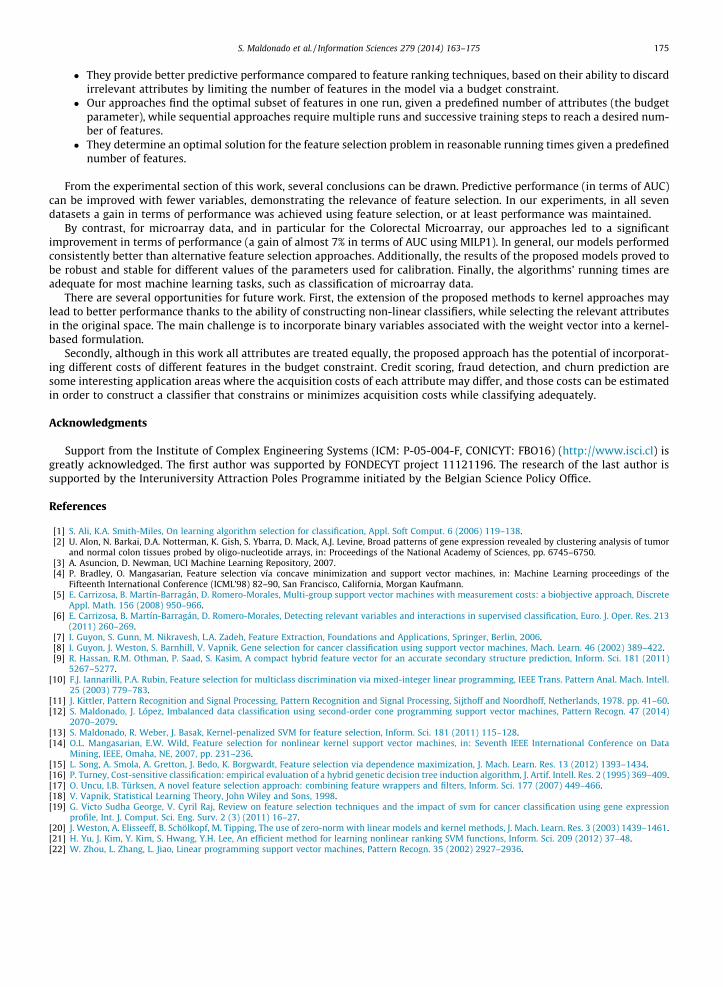
� They provide better predictive performance compared to feature ranking techniques, based on their ability to discardirrelevant attributes by limiting the number of features in the model via a budget constraint.

� Our approaches find the optimal subset of features in one run, given a predefined number of attributes (the budgetparameter), while sequential approaches require multiple runs and successive training steps to reach a desired num-ber of features.

� They determine an optimal solution for the feature selection problem in reasonable running times given a predefinednumber of features.

From the experimental section of this work, several conclusions can be drawn. Predictive performance (in terms of AUC)can be improved with fewer variables, demonstrating the relevance of feature selection. In our experiments, in all sevendatasets a gain in terms of performance was achieved using feature selection, or at least performance was maintained.

By contrast, for microarray data, and in particular for the Colorectal Microarray, our approaches led to a significantimprovement in terms of performance (a gain of almost 7% in terms of AUC using MILP1). In general, our models performedconsistently better than alternative feature selection approaches. Additionally, the results of the proposed models proved tobe robust and stable for different values of the parameters used for calibration. Finally, the algorithms’ running times areadequate for most machine learning tasks, such as classification of microarray data.

There are several opportunities for future work. First, the extension of the proposed methods to kernel approaches maylead to better performance thanks to the ability of constructing non-linear classifiers, while selecting the relevant attributesin the original space. The main challenge is to incorporate binary variables associated with the weight vector into a kernel-based formulation.

Secondly, although in this work all attributes are treated equally, the proposed approach has the potential of incorporat-ing different costs of different features in the budget constraint. Credit scoring, fraud detection, and churn prediction aresome interesting application areas where the acquisition costs of each attribute may differ, and those costs can be estimatedin order to construct a classifier that constrains or minimizes acquisition costs while classifying adequately.

Acknowledgments

Support from the Institute of Complex Engineering Systems (ICM: P-05-004-F, CONICYT: FBO16) (http://www.isci.cl) isgreatly acknowledged. The first author was supported by FONDECYT project 11121196. The research of the last author issupported by the Interuniversity Attraction Poles Programme initiated by the Belgian Science Policy Office.

References

[1] S. Ali, K.A. Smith-Miles, On learning algorithm selection for classification, Appl. Soft Comput. 6 (2006) 119–138.[2] U. Alon, N. Barkai, D.A. Notterman, K. Gish, S. Ybarra, D. Mack, A.J. Levine, Broad patterns of gene expression revealed by clustering analysis of tumor

and normal colon tissues probed by oligo-nucleotide arrays, in: Proceedings of the National Academy of Sciences, pp. 6745–6750.[3] A. Asuncion, D. Newman, UCI Machine Learning Repository, 2007.[4] P. Bradley, O. Mangasarian, Feature selection vía concave minimization and support vector machines, in: Machine Learning proceedings of the

Fifteenth International Conference (ICML’98) 82–90, San Francisco, California, Morgan Kaufmann.[5] E. Carrizosa, B. Martín-Barragán, D. Romero-Morales, Multi-group support vector machines with measurement costs: a biobjective approach, Discrete

Appl. Math. 156 (2008) 950–966.[6] E. Carrizosa, B. Martín-Barragán, D. Romero-Morales, Detecting relevant variables and interactions in supervised classification, Euro. J. Oper. Res. 213

(2011) 260–269.[7] I. Guyon, S. Gunn, M. Nikravesh, L.A. Zadeh, Feature Extraction, Foundations and Applications, Springer, Berlin, 2006.[8] I. Guyon, J. Weston, S. Barnhill, V. Vapnik, Gene selection for cancer classification using support vector machines, Mach. Learn. 46 (2002) 389–422.[9] R. Hassan, R.M. Othman, P. Saad, S. Kasim, A compact hybrid feature vector for an accurate secondary structure prediction, Inform. Sci. 181 (2011)

5267–5277.[10] F.J. Iannarilli, P.A. Rubin, Feature selection for multiclass discrimination via mixed-integer linear programming, IEEE Trans. Pattern Anal. Mach. Intell.

25 (2003) 779–783.[11] J. Kittler, Pattern Recognition and Signal Processing, Pattern Recognition and Signal Processing, Sijthoff and Noordhoff, Netherlands, 1978. pp. 41–60.[12] S. Maldonado, J. López, Imbalanced data classification using second-order cone programming support vector machines, Pattern Recogn. 47 (2014)

2070–2079.[13] S. Maldonado, R. Weber, J. Basak, Kernel-penalized SVM for feature selection, Inform. Sci. 181 (2011) 115–128.[14] O.L. Mangasarian, E.W. Wild, Feature selection for nonlinear kernel support vector machines, in: Seventh IEEE International Conference on Data

Mining, IEEE, Omaha, NE, 2007, pp. 231–236.[15] L. Song, A. Smola, A. Gretton, J. Bedo, K. Borgwardt, Feature selection via dependence maximization, J. Mach. Learn. Res. 13 (2012) 1393–1434.[16] P. Turney, Cost-sensitive classification: empirical evaluation of a hybrid genetic decision tree induction algorithm, J. Artif. Intell. Res. 2 (1995) 369–409.[17] O. Uncu, I.B. Türksen, A novel feature selection approach: combining feature wrappers and filters, Inform. Sci. 177 (2007) 449–466.[18] V. Vapnik, Statistical Learning Theory, John Wiley and Sons, 1998.[19] G. Victo Sudha George, V. Cyril Raj, Review on feature selection techniques and the impact of svm for cancer classification using gene expression

profile, Int. J. Comput. Sci. Eng. Surv. 2 (3) (2011) 16–27.[20] J. Weston, A. Elisseeff, B. Schölkopf, M. Tipping, The use of zero-norm with linear models and kernel methods, J. Mach. Learn. Res. 3 (2003) 1439–1461.[21] H. Yu, J. Kim, Y. Kim, S. Hwang, Y.H. Lee, An efficient method for learning nonlinear ranking SVM functions, Inform. Sci. 209 (2012) 37–48.[22] W. Zhou, L. Zhang, L. Jiao, Linear programming support vector machines, Pattern Recogn. 35 (2002) 2927–2936.