Federal Reserve Bank of Minneapolis

Fail 1999

Maintenance and Repair Too Big to Ignore (p. 2) Ellen R. McGrattan James A. Schmitz, Jr.

Explaining the Fiscal Theory of the Price Level (p. 14) Narayana Kocherlakota Christopher Phelan

Federal Reserve Bank of Minneapolis

Quarterly Review vol. 23, no. 4 ISSN 0271-5287

This publication primarily presents economic research aimed at improving policymaking by the Federal Reserve System and other governmental authorities.

Any views expressed herein are those of the authors and not necessarily those of the Federal Reserve Bank of Minneapolis or the Federal Reserve System.

Editor: Arthur J. Rolnick Associate Editors: Edward J. Green, Patrick J. Kehoe,

Warren E. Weber Economic Advisory Board: V. V. Chari, Harold L. Cole,

Thomas J. Holmes, Patrick J. Kehoe Managing Editor: Kathleen S. Rolfe

Article Editors: Kathleen S. Rolfe, Jenni C. Schoppers Production Editor: Jenni C. Schoppers

Designer: Phil Swenson Typesetters: Mary E. Anomalay, Sandra E. Zilka

Circulation Assistant: Elaine R. Reed

The Quarterly Review is published by the Research Department of the Federal Reserve Bank of Minneapolis. Subscriptions are available free of charge.

Quarterly Review articles that are reprints or revisions of papers published elsewhere may not be reprinted without the written permission of the original publisher. All other Quarterly Review articles may be reprinted without charge. If you reprint an article, please fully credit the source—the Minneapolis Federal Reserve Bank as well as the Quarterly Review—and include with the reprint a version of the standard Federal Reserve disclaimer (italicized above). Also, please send one copy of any publication that includes a reprint to the Minneapolis Fed Research Department.

Electronic files of Quarterly Review articles are available through the Minneapolis Fed's home page on the World Wide Web: http://www.minneapolisfed.org.

Comments and questions about the Quarterly Review may be sent to

Quarterly Review Research Department Federal Reserve Bank of Minneapolis P. O. Box 291 Minneapolis, Minnesota 55480-0291 (Phone 612-204-6455 / Fax 612-204-5515).

Subscription requests may also be sent to the circulation assistant at elaine.reed@mpls.frb.org; editorial comments and questions, to the managing editor at ksr@res.mpls.frb.fed.us.

Federal Reserve Bank of Minneapolis Quarterly Review Fall 1999

Explaining the Fiscal Theory of the Price Level

Narayana Kocherlakota* Associate Consultant Research Department Federal Reserve Bank of Minneapolis and Professor Department of Economics University of Minnesota

Christopher Phelan* Economist Research Department Federal Reserve Bank of Minneapolis

How can governments influence inflation rates? Econo-mists' standard answer is that the central bank controls the inflation rate through its ability to control the money supply. In particular, if output grows at y percent per year and the money supply grows at |u percent per year, then, at least over sufficiently long periods of time, prices will grow at ((J-y) percent per year. Simply put, the inflation rate is determined by the change in the rel-ative scarcities of money and goods.

Unfortunately, there is a large hole in this simple, stat-ic reasoning. How much money a household wants to hold today depends crucially on that household's beliefs about future inflation. As it turns out, this dependence of current money demand on beliefs about future inflation creates the possibility of a large number of equilibrium paths of inflation rates, besides the one in which prices grow at (ja-y) percent. (See Obstfeld and Rogoff 1983, for example.) Thus, control of the money supply alone is not sufficient to pin down the time path of the inflation rate.

This analysis suggests the following important ques-tion: Can the government use some other policy instru-ment, such as taxes or debt policy, in conjunction with monetary policy to determine the time path of the infla-tion rate? In an important recent paper, Woodford (1995) proposes a new theory of price determination, the fiscal theory of the price level. He argues that the government's choice of how to finance its debt plays a crucial role in the determination of the time path of the inflation rate.1

In this article, we explain this theory. We make three main points. First, we show that according to Wood-ford's (1995) theory, fiscal policy affects inflation rates if and only if the government can behave in a fundamen-tally different way from households. Households must satisfy intertemporal budget constraints, no matter what price paths they face. Woodford (1995) argues that the government does not face this same requirement; the government can follow non-Ricardian fiscal policies un-der which the intertemporal budget constraint is satisfied for some, but not all, price paths. Following Woodford (1995), we show that fiscal policy can affect inflation rates if and only if the government can use non-Ricar-dian policies.

Why can the government influence inflation rates when it uses non-Ricardian policies? We show that if the government's intertemporal budget constraint is not satisfied for a price path, then that price path cannot be an equilibrium (because such a path is inconsistent with market-clearing and household optimality). Hence, the government can reject any price path as an equilibrium

•The authors' understanding of the issues in this paper has benefited greatly from discussions with Larry Jones. The authors also wish to thank V. V. Chari, John Cochrane, Harold Cole, and Warren Weber for helpful comments and Kathy Rolfe and Jenni Schoppers for expert editorial advice.

'See Leeper 1991, Sims 1994, McCallum 1998, Buiter 1999, and Cochrane 1999 for other discussions of the fiscal theory.

14

Narayana Kocherlakota, Christopher Phelan Fiscal Theory of the Price Level

by guaranteeing that its intertemporal budget constraint is not satisfied along that price path.

Our second point concerns a natural question: Can the government implement non-Ricardian policies, even though households cannot? We argue that this question cannot be answered using data. Whether a fiscal policy is non-Ricardian concerns the government's behavior at unobserved price paths; therefore, such a determination is nontestable. Fundamentally, then, whether the govern-ment can follow a non-Ricardian policy is a religious, not a scientific, question.

Finally, we demonstrate that the predictions of a spe-cific popular non-Ricardian fiscal policy for inflation are highly counterintuitive. In particular, we show that under this non-Ricardian policy, one-time decreases in the mon-ey supply can lead to hyperinflations. This is in stark con-trast to the usual monetarist intuition under which one-time decreases in the money supply have no effect on long-run inflation rates.

We proceed in three parts. First, we show that stan-dard monetary models have an infinite number of pre-dictions for the time path of inflation rates. Our analysis closely follows that of Obstfeld and Rogoff (1983). Next, we demonstrate how the fiscal theory of the price level serves to shrink the set of predictions by allowing the government to use non-Ricardian policies. Finally, we argue that the fiscal theory is not falsifiable, and we con-sider its implications for the consequences of a once-and-for-all decrease in the money supply.

On the Indeterminacy of Monetary Equilibria In this section, we present an example economy, origi-nally due to Obstfeld and Rogoff (1983), that shows how standard monetary models have a continuum of equilib-rium time paths for the inflation rate.2

In our example economy, time is discrete and infinite. There is a continuum of identical households. The house-holds are initially endowed with M_x dollars and with a constant stream of y perishable consumption goods. In our example, we assume that the money supply does not change over time.

In each period, households exchange money, nominal bonds, and consumption in a competitive market. In this market, households face a sequence of flow budget con-straints (for all t > 0) of the following form:

(1) Ptct + Mt + Bt< Mt_x + Rt_xBt_x + Pty

with ct and M, > 0, Z?_, = 0, and M_x given. In this mar-ket, ct is the amount of consumption goods consumed by the household in period f, Mt is the amount of dollars held by the household at the end of period t, Bt is the amount of the nominal bonds held by the household at the end of period t, Rt is the number of dollars a bond pays in period t + 1, and Pt is the price of consumption in terms of dollars in period t. (Here and throughout the article, uppercase letters refer to nominal variables, and lowercase letters to real variables.)

Households also face a borrowing condition that for all t>0,

(2) Mt_x + Rt_xBt_x + Y^ylWoKs * 0.

In words, this condition requires that the household's wealth at the end of period t, including the present value of its income stream, be nonnegative. This condition eliminates Ponzi schemes (or financing unlimited con-sumption by running Bt to negative infinity).

If Pt > 0 for all t, then the price of a period t dollar in terms of period 0 dollars is l/YYsZl

0Rs. Given this, the formulation above of a household's budget set as a se-quence of flow budget constraints (1) and a borrowing condition (2) is equivalent to the perhaps more familiar formulation of a consumer's budget set as one in which the value of expenditures in terms of some numeraire good equals the value of resources in terms of that same numeraire. That is, constraint (1) and condition (2) de-fine the same set of feasible consumption and money sequences as the present-value budget condition

(3) E > - i w + p ^ y u 1 - 1 ^

Here, the left side is the value of the household's net purchases of money and the household's consumption, while the right side is the value (in terms of period 0 money) of the household's endowment stream.

Each household has the same preferences over streams of consumption and real balances:

w E^P'MC,) + w n

2This analysis is close to that of McCallum (1998).

15

Here, 0 < P < 1. Also, the utility functions over consump-tion and real balances, u and v, are assumed twice dif-ferentiable, strictly increasing, and strictly concave, with u\0) = oo

The household seeks to maximize this objective func-tion, subject to equations (1) and (2). If the borrowing condition (2) ever binds, the household must have ct = 0 in all future periods; therefore, the assumption that u\0) = oo ensures that (2) never binds.

An equilibrium is a sequence {P,,/?,},0^ °f nominal prices and interest rates such that, given this sequence, households find it optimal to choose to hold the supply M_, of dollars and eat y of the consumption goods in each period (and thus set Bt = 0 each period). Examina-tion of the first-order conditions delivers that any posi-tive sequence is an equilibrium if and only if condition (3) holds with equality and for all t > 0,

(5) v\MJPt) = u\y)[\-\/Rt]

(6) Rt = (\/$)(PtJPt).

The present-value budget condition (3) holding with equality is equivalent to the flow budget constraint (1) holding with equality and the limiting condition

(7) XxmT_SMT_x + RT-XBT_xmT^Rs = 0.

In this economy, output does not grow and money does not grow. Hence, the standard, static thinking about inflation would say that nominal prices should not grow. There is indeed an equilibrium of this form. In this equi-librium, for all

(8) P, = P*

(9) Rt= 1/(3

(10) v'(M_l/P*) = (\-$)u'(y).

(Note that in this equilibrium, the value of money P* is inversely proportional to the supply of money M_,.)3

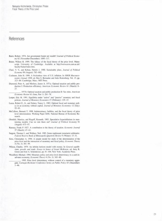
Under a wide variety of assumptions about u and v, however, there is a continuum of other equilibria. To see this, solve equation (5) for Pt+l after imposing equation (6), yielding

(11) Pt+l= pP,[ 1 - (v\MJPt)/u\y))Y\

If we assume that4

(12) u(c) = log(c)

(13) v(M/P) = \og(y+M/P)

we have the following difference equation:

(14) Pt+l = p/>,[l + (Pty/M_{)].

The accompanying chart displays this function. It has a fixed point at zero, and P = [(1-(3)/p](M_ ,/>')• Further, for all Pt > P\ Pt+l > Pt; thus, Pt becomes arbitrarily large (or money becomes valueless). For any P0 > P*, the price path constructed in this manner [along with Rt = (1/p)(PtJPt)] is an equilibrium. (If P0 < P\ equa-tion (14) implies that prices go to zero, or money be-comes infinitely valuable. Given this, however, condition (7) is violated; thus, these paths are not equilibria.)

Thus, given our assumption about household prefer-ences, there is a continuum of equilibria in this economy. We can easily show that this result can be obtained for ar-bitrary specifications of the endowment process and for arbitrary growth in the money supply. Nor is this result special to money-in-the-utility-function models. The mul-tiplicity of equilibria also occurs in cash-in-advance mod-els (Wilson 1979) and in cash-credit models (Woodford 1994).

This multiplicity of equilibria should not be surpris-ing. Unlike a stock which pays dividends or a piece of art which the owner can enjoy looking at, money in this economy is a purely speculative asset. In every period, a household's utility from holding money depends only on how much other households value money relative to the consumption good. (That is, the household values real, as opposed to nominal, balances.) The equilibria in which P0 > P (and thus Pt goes to infinity) are essentially spec-ulative hyperinflations. Even though every household un-derstands that money is becoming valueless, households still hold positive but shrinking real balances because of the utility those real balances bring.

3 In fact, there are two stationary equilibria, but the second does not fit our choice of numeraire. If the price of money in terms of consumption is zero in all periods (or money is worthless), then all households receive no utility from holding money and thus are unwilling to pay a positive price to hold it.

4Putting the endowment y in the utility function for money guarantees that v\MIP)lu'{y) < 1 for all M/P > 0. This ensures that prices never become negative.

16

Narayana Kocherlakota, Christopher Phelan Fiscal Theory of the Price Level

The Difference Equation for Prices In the Example Economy

Fiscal Policy and Equilibrium In this section, we introduce fiscal policy into our exam-ple economy. We show that various formulations of fis-cal policy have important consequences for the ability of the government to influence inflation.

Formulating Fiscal Policy First, we introduce a government into our economy, along with the elements of fiscal policy. For simplicity, and because it makes no difference in understanding the issues we address, we assume that government spending, in real terms, is constant at the level g. Suppose house-holds are initially endowed with R_XB_X dollars of nomi-nal government debt (where R_\B_X can be negative). At the beginning of each period t, the government imposes lump-sum taxes xt (again, i t can be negative), retires its existing debt, issues new debt, and prints new money.

Formally, the households now face a sequence of flow budget constraints of the following form:

(15) Ptct + Mt + Bt< Mt_x + Rt_xBt_x + Pt(y-%,)

with ct and Mt > 0 and with R_XB_, and M_x given. Again, to ensure that the household does not keep bor-rowing without limit, we impose the following borrow-ing condition for all t > 0:

(16) MM+R,_,B,_X+5;>(+.(y-Tf+.)/ni:X, * o.

This condition, again, never binds at a household's opti-mum.

The key now is how we specify government fiscal policy. DEFINITION. A policy n is a function that maps positive price sequences P = into sets of sequences (t,R,B,M) = {TrRrBrMt}7=0 such that if (x,R,B,M) e n ( P ) , then for all t,

(17) Ptxt + Bt + Mt = Ptg + Rt_xBt_x + Mt_x.

Thus, a government policy specifies a set of possible tax, nominal interest rate, debt, and money supply sequences for each possible price sequence with a re-striction that these sequences must satisfy a flow budget constraint. (Note that Af_, and are not under the control of the government.) We emphasize that a policy is a set of sequences (t,R,B,M) for each price sequence P as opposed to a single sequence for each P because a government can choose to let an element of (tt,Rt,Bt,Mt) be unspecified. For instance, a government can decide to let the "market" determine the nominal return on bonds Rr the quantity of bonds Bt, or the money supply Mr

We purposely use a quite general definition of poli-cy. For instance, in an approach popularized by Ramsey (1927) [and followed up by Diamond and Mirrlees (1971a, b), Lucas and Stokey (1983), and Chari and Kehoe (1990)], a policy would be simply a sequence of tax rates and money supplies. Putting such a policy in our framework would involve leaving nominal interest rates and bonds unspecified and having the same se-quence of tax rates and money supplies for all price se-quences. A policy could instead involve complicated feedback rules from prices to money supplies or taxes. Further, a policy could have the government explicitly set the nominal interest rate, either as simply an exoge-nous sequence or through some feedback rule from prices to nominal interest rates. Our formulation allows all of these possibilities. Our formulation of policy does

17

not allow explicit price-setting of the consumption good by the government. This restriction is in keeping with the spirit of the fiscal theory of the price level, which takes as given that the government can influence the price level only indirectly through monetary and fiscal policy.

Given our notion of policy and given that ct = y - g for all t from the resource constraint, an equilibrium in this economy is a sequence {Pt,xrRrBt,Mt}Zo suc^ that the following five conditions hold:

(18) v'(Mt/Pt) = u(y-g)[\-\/Rt]

(19) Rt = (\/$)(PtJPt)

(20) l i m ^ J M ^ + R t _ , B t J YlllX = 0

(21) Pt(y-g) + Bt + Mt = Pt(y-T{) + Rt_xBt_x + Mt_x

(22) (t,R,B,M) in n(P).

The first two conditions are from the household's first-order conditions. The next requirement is the house-hold's transversality condition. The fourth condition says that the household's flow budget constraint is satisfied with equality. The final condition requires that the gov-ernment follow its policy n.

As before, if the limiting condition on household wealth is satisfied and the sequence of household bud-get constraints holds with equality, then the household's infinite-period budget constraint

(23) E~0t(l - 1 / W + P,(y-g)VY^R,

* Y^JP.iy-V'WM + * < + M ,

holds with equality (and vice versa).

Two Types of Government Policy What types of policy should economists be willing to consider? By requiring policies to satisfy a government's flow budget constraint, we have already imposed an opinion that those policies which violate such a con-straint are nonsensical. Whether this is the only require-ment we need to impose on policy is at the heart of un-derstanding the fiscal theory of the price level. Here and in the next subsection, we formally consider the implica-tions of further requiring that a policy always balance the government's budget in the "long run." We argue that

imposing such a restriction makes fiscal policy, in an im-portant sense, irrelevant.

The preceding formalization of policy specifies a set of possible actions for every specification of prices in this economy. Thus, a policy looks a lot like a con-sumer's excess demand correspondence in neoclassical economics. But there is a key difference: a demand correspondence must satisfy the requirement that for all prices, the value of a consumer's excess demand is ze-ro. In this case, this implies that a consumer's infinite-period budget constraint holds with equality. Following Woodford (1995), we use the term Ricardian to refer to policies that satisfy an equivalent restriction for the gov-ernment as well.

To define the notion of a Ricardian policy, we must first introduce an infinite-horizon budget constraint for the government. Analogous to the household's, the gov-ernment's infinite-horizon budget constraint

(24) ( £ , ! 0 [ a - i / w ] / n ; : i ^ - M ,)

requires that the present discounted value of government revenues (including seigniorage) be at least as large as the government's obligations. Like the household's, the government's infinite-horizon budget constraint holds with equality if and only if the government's flow bud-get constraint holds with equality and the limiting condi-tion

(25) li mT^{MT_x + Rt_xBt_x)ITIts~JqRs = 0

is satisfied. We say a policy n is Ricardian if for all P and for

all (i,R,B,M) in n(P), the government's infinite-horizon budget constraint is satisfied with equality. Equivalently, a policy n is Ricardian if and only if for all P and for all (t,R,B,M) in n(P), condition (25) holds. This latter formulation of Ricardian policy will be more convenient for some purposes.

What is an example of a Ricardian policy? Suppose that for all P, (x,R,ByM) is in Yl(P) if and only if for all t,

(26) Tt = (Rt_ry)(BtJPt) + g,y<l

(27) Rt > 1 + r|, r| > 0

(28) Bt = YB_{

18

Narayana Kocherlakota, Christopher Phelan Fiscal Theory of the Price Level

(29) Mt = M_v

Under this policy, the government always collects enough in taxes to pay g, its interest obligations, and fraction (1-y) of its nominal debt. (If B_, is negative, then the government collects less than g in taxes and uses the interest on its net assets to fund g.) Because the government's debt is shrinking over time, the policy is Ricardian.

What is an example of a non-Ricardian policy? Sup-pose that for an arbitrary Pt {x,R,B,M) is in FI(P) if and only if for all t,

(30) x, = g + 8, e > 0

(31) Rt> 1 +ti,TI>0

(32) Bt = Rt_\Bt_x - eP\

(33) Mt-M_v

Under this policy, the government rolls over all but ePt of its initial debt in every period. To see that this policy is not Ricardian, suppose that Pt = P and Rt = 1/(3 for all t. Then the government's infinite-horizon budget con-straint can only be satisfied if

(34) R_xB_x=zPI{ 1-p).

Only one value of P satisfies equation (34). Hence, the policy is not Ricardian, because the infinite-horizon bud-get constraint is not satisfied for all price level sequences.

Equilibrium With Ricardian and Non-Ricardian Fiscal Policies In this subsection, we first consider the set of equilibri-um prices under the two example policies. We show that under our example Ricardian policy (and under Ri-cardian policies in general), fiscal policy is irrelevant. We then show precisely how fiscal policy can determine prices when non-Ricardian policies are allowed.

• Ricardian Policy Recall our earlier example policy which specifies that for all P, (x,R,B,M) is in Yl(P) if and only if for all t,

(35) Tt = (Rt_-y)(Bt_{/Pt) + g,y<l (36)

(37) Bt =

(38) Mt = M_v

As in our earlier example, we assume that

(39) u(c) = log(c) (40) v(M/P) = \og(y-g+M/P).

We can use our reasoning of the preceding section to show that under our example Ricardian policy, any price sequence of the form

(41) P0>P*

such that

(42) (1-p ) = P\y-g)/M_{

(43) Pt+l = pP,[l + Pt(y-g)/M_{]

is an equilibrium price sequence regardless of the initial debt We can see this by noting that any such se-quence, together with the sequences defined by the poli-cy, as well as

(44) Rt = (l/p)(P,+,//>,)

satisfy the equilibrium conditions. Thus, under the Ricardian policy, all of the equilibri-

um price sequences derived earlier are still equilibria. This is an example of a much more general principle: Every Ricardian policy which specifies the same se-quence of money supplies has the same set of equilibri-um price sequences. The initial government debt and the timing of taxes is, in this important sense, irrelevant. (That is, Ricardian equivalence holds.) The initial gov-ernment debt held by households, R_\B_X, does not affect real household wealth because the present value of taxes (over and above g) must always equal it. To paraphrase Barro (1974), government bonds are not net wealth and thus affect nothing of interest.

• Non-Ricardian Policy Now suppose that the government follows the policy n such that (t,R,B,M) is in Yl(P) if and only if for all t,

Rt > 1 + r|, r| > 0 (45) T, = g + £, 8 > 0

19

(46) Rt> 1 + r|, r| > 0

(47) Bt = Rt_xBt_x - ePt

(48) Mt = M_,.

Assume, as before, that

(49) u(c) = log(c)

(50) v(M/P) = \og(y-g+M/P).

Again, pick an arbitrary P0 > P\ and consider the se-quence Pt defined recursively by the household's first-order condition:

(51) Pt+, = $P\\+Pt{y-g)IM_xl

Under the above Ricardian policy, this sequence is an equilibrium for any choice of P0 > P*. However, under the non-Ricardian policy, such a sequence is an equi-librium for only one possible P0. To see this, note that household optimization requires that for all price se-quences P, the household's infinite-period budget con-straint (23) must hold with equality, or

(52) )M, + p,c,]/

= Y^JP^y-^U'M + 1 + m_v

Imposing the equilibrium condition ct = y - g and re-arranging equation (52) delivers the government budget constraint used in the definition of a Ricardian policy:

(53) - w J

+ = + £ , > , g / n : : x

It is important to note that while equation (53) was in-troduced in the discussion of Ricardian policies as a constraint on government policy (for all price sequences P), it has been separately derived as an equilibrium con-dition using only household optimization and market-clearing.5 Further imposing the non-Ricardian policy above (Af, = and xt = g + £), we have

(54) R_tB_t

as an equilibrium condition. Finally, imposing the equi-librium condition that Rt = (1/(3)(Pt+]/Pt) implies

(55) R.{BJP0 = e/(l-P)

as an equilibrium condition. Here, the left side is the real period 0 value of the initial government debt and the right side is the present value of the government's real surpluses. If R_\B_{ is positive, a unique P0 is pinned down. If this unique P0 > P*, then a unique equilibrium is selected from the set of equilibria generated by our example Ricardian policy.6

More generally, for a policy to be non-Ricardian, by definition, price sequences P must exist for which the government's infinite-period budget constraint does not hold with equality. Since we derived from household op-timization and goods market-clearing that for any equi-librium price sequence, the government's infinite-period budget constraint must hold, these price sequences are immediately rejected as equilibria.

Thus, at its very core, a non-Ricardian policy is an equilibrium rejection device. To eliminate all equilibria, choose a policy for which the government's infinite-period budget constraint is violated under all price se-quences P. To select a particular equilibrium (or subset of equilibria) of a Ricardian policy, specify that the gov-ernment act the way it would under the Ricardian policy for that particular price sequence (or subset of sequenc-es) and that it act in a way which violates its infinite-period budget constraint for all other price sequences. Because it is the specification of government fiscal poli-cy which eliminates some price sequences as potential equilibria, in some sense, it is this policy which "causes" the remaining price sequences to be candidate equilibria. This is the rationalization for the term fiscal theory of the price level.1

Implications In this section, we consider the empirical implications, or testability, of the fiscal theory of the price level. To this end, consider data on sequences (PM,B,yyg}x). (We

5This is Walras' law. If the budget constraint holds with equality for all but one agent in the economy and markets clear, the budget constraint holds with equality for the last agent.

6Perhaps we should particularly note that this non-Ricardian policy eliminates the worthless-money equilibrium described in footnote 3. This implies that a non-Ricardian policy can "cause" money to have value. In this example, money has to have value so that the government surpluses have a real debt to pay off.

7That allowing non-Ricardian policies is equivalent to allowing governments to simply reject price vectors as equilibria is not specific to the example economy pre-sented here. This equivalence holds for any economy in which household optimiza-tion implies that the household's budget constraint is satisfied with equality.

20

Narayana Kocherlakota, Christopher Phelan Fiscal Theory of the Price Level

could even allow these sequences to be infinite.) The fiscal theory is of interest only if we believe that gov-ernments sometimes follow non-Ricardian policies. Can we identify whether these data were generated by a Ri-cardian or non-Ricardian policy? If the data fit our defi-nition of an equilibrium, the answer is simply no. The distinction between Ricardian and non-Ricardian policies is precisely over how the government would have acted for price sequences other than P. A non-Ricardian policy implies that the government would have acted in a way in which it didn't satisfy its infinite-period budget con-straint with equality. Would it have? We cannot know because we only see how it acted under P. The fiscal theory of the price level is not falsifiable. (Arguments similar to this are in Cochrane 1999.)

However, a joint hypothesis, such as that the govern-ment has a particular class of desired outcomes and uses non-Ricardian policies to achieve them, is falsifiable. For instance, we could assert that governments use non-Ricardian policies to select the stationary equilibria asso-ciated with stationary policies, and then we could see if governments with stationary monetary policies tend to have stationary prices. The difficulty with this approach is that while such a joint hypothesis is falsifiable, it can't be distinguished from any other equilibrium selection de-vice. For instance, we could hypothesize that when sta-tionary equilibria exist, they are the equilibria that occur simply because stationarity is the natural focal point of beliefs. If our tests do not reject stationarity, no further tests will be able to say whether stationary price paths occur because of non-Ricardian policies or some other reason.

Whether a government is following a particular non-Ricardian policy is also falsifiable. Consider, for in-stance, our example non-Ricardian policy in which the government follows the same tax and spending policy regardless of the price sequence. Leeper (1991) calls this a passive policy. We interpret the empirical exercises in papers such as Cochrane 1999 as examining the implica-tions of this kind of policy.

We can see this by examining the general form of equation (55) (the present value of the stream of real government surpluses must equal the real government debt) and considering two alternative policies. In one, the government taxes g + 8 in every period, as in our example economy. In the other, the government taxes g + 2 8 in period t = 0 (in which case, B0 = -2eP0) and g + e in every subsequent period. If taxes are

8 in period 0, then equation (55) is unchanged. If taxes are 28, then equation (55) becomes

(56) R_}BJP0 = e+[e/(l-p)]

which solves for a lower P0. Thus, the above policy ap-pears to predict that if taxes are increased, current prices go down. This prediction would extend to a more formal version of our example with stochastic policy—taxes would be negatively correlated with prices.

Suppose, then, that we observe a systematic negative correlation between taxes and prices. Is this evidence that the government is using a non-Ricardian policy, and so the fiscal theory of the price level is at work? It is true that under a Ricardian policy, the set of equilibrium price paths is unaffected by taxes. However, only one element of this set actually occurs in equilibrium. It is certainly possible that while the set is unchanged, the selection of an equilibrium price path from that set is based on gov-ernment tax policy, creating a negative correlation be-tween taxes and prices. Thus, such a negative correlation is not evidence against the government's using a Ricar-dian policy. As we argued above, the only way to know if the government is using a non-Ricardian policy is to know whether the government's budget constraint is sat-isfied for unobserved prices. This is impossible.8

A Concluding Example We have argued that the fiscal theory of the price level is, at its core, a device for selecting equilibria from the continuum which can exist in monetary models. We can contrast this equilibrium selection device with another, more traditional, selection device. This alternative mone-tarist selection device rules out equilibria with purely speculative time trends in velocity. (For examples in which technology and the money supply are constant, the monetarist device implies a constant price level.) For general specifications of initial debt, the monetarist se-lection device conflicts with the fiscal theory device. The following example, we believe, questions the plau-sibility of the fiscal theory device.

Consider the following. An outside observer of the economy sees the stationary price path and government

8 Another reason for a negative correlation between taxes and prices is pointed out by Sargent and Wallace (1985). They argue that a decrease in the government's debt today lowers the likelihood of increases in the money supply in the future.

21

actions consistent with equilibrium and our example non-Ricardian policy. That is, the observer's data on the econ-omy for periods t = 0, 1,2,... (7-1) are

(57) pt = p() = [(\-mwjy

(58) x, = g + 8, e > 0

(59) Rt= 1/(3

(60) Bt = Rt_\Bt_x - zPt

(61) Mt = M_,.

As we stressed earlier, the outside observer could have (at least) two explanations for these data. One is that the government is using our example non-Ricardian policy. The other is that the government is using some Ricardian policy, and the stationary equilibrium is being selected from the set of possible equilibria.

Next suppose that in period T, the government sur-prisingly confiscates a fraction jc of the money supply. (In our notation, this fraction is bought using an increase in period T lump-sum taxes.) The government then cred-ibly commits to using the same policy n as before, with the one change that the money supply stays fixed at its new low level.

However, the outside observer does not know wheth-er the policy n is Ricardian or not. Suppose first that n is Ricardian and that the monetarist selection device is at work. Then, in period T and thereafter

(62) Pt = />** = [(l-mm-x)M_{/yl

Prices fall by the same fraction x as the money supply and then stay constant. Of course, because this price fall implies an increase in the real value of the government debt, the government's taxes must rise at some point in the future to satisfy the government's budget constraint.

In contrast, suppose that n is our example non-Ricardian policy. Then, if we consider period T as period 0, equation (55) becomes

(63) Rt_xBtJPt = e/(l-fi).

Neither the real present value of budget surpluses nor the nominal debt is affected by this confiscation; thus, the value for PT is unaffected. However, the stationary equi-librium price has fallen to P**. Because the initial price

level PT under the non-Ricardian policy is greater than P \ the result is hyperinflation.

Thus, the two equilibria selection devices produce radically different consequences for this policy change of a one-time decrease in the money supply. The monetarist device predicts a one-time decrease in the price level, equal in percentage terms to the decrease in the money supply. Given our example policy, the fiscal theory de-vice predicts a speculative hyperinflation. Which predic-tion seems more plausible? You decide.

Conclusion Economists have known for some time that, in general, monetary model economies have a large number of equi-librium price paths. We have argued that the traditional, and often unstated, selection device (which we call mon-etarist) rules out equilibria with purely speculative time trends in velocity. The fiscal theory of the price level is an alternative selection device. The key force behind the fiscal theory is that a government is fundamentally dif-ferent from households. Households need to satisfy their budget constraint for all prices, regardless of whether or not those prices are equilibria. A government does not. Further, a government's pledge not to satisfy its budget constraint for a price path is, mechanically, a rejection by the government of that price path as an equilibrium. These selection devices will be in conflict unless, of course, governments choose only equilibria which the monetarist device would have chosen anyway.

More fundamentally, the fiscal theory is about the behavior of the government for unobserved prices. As we have pointed out, it is therefore impossible to decide, using data from a particular equilibrium, whether the fiscal theory has served to select that equilibrium. This makes the broad question of whether governments can follow non-Ricardian policies a fundamentally religious, not scientific, issue.

For our example policy of constant taxes and constant money, we show that the fiscal theory predicts a specula-tive hyperinflation in response to a once-and-for-all de-crease in the money supply. In contrast, the standard monetarist selection device predicts a once-and-for-all decrease in the price level. To take the fiscal theory seriously, we must believe that a government could ac-tually choose the hyperinflation outcome by following our example policy. One cannot "believe in" the fiscal theory device and the monetarist device simultaneously. We choose to believe in the latter.

22

Narayana Kocherlakota, Christopher Phelan Fiscal Theory of the Price Level

References

Barro, Robert. 1974. Are government bonds net wealth? Journal of Political Econo-my 82 (November-December): 1095-117.

Buiter, Willem H. 1999. The fallacy of the fiscal theory of the price level. Manu-script. University of Cambridge. Available at http://www.econ.cam.ac.uk/ faculty/buiter/index.htm.

Chari, V. V., and Kehoe, Patrick J. 1990. Sustainable plans. Journal of Political Economy 98 (August): 783-802.

Cochrane, John H. 1999. A frictionless view of U.S. inflation. In NBER Macroeco-nomics Annual 1998, ed. Ben S. Bernanke and Julio Rotemberg, Vol. 13, pp. 323-84. Cambridge, Mass.: MIT Press.

Diamond, Peter A., and Mirrlees, James A. 1971a. Optimal taxation and public pro-duction I: Production efficiency. American Economic Review 61 (March): 8-27.

. 1971b. Optimal taxation and public production II: Tax rules. American Economic Review 61 (June, Part 1): 261-78.

Leeper, Eric M. 1991. Equilibria under "active" and "passive" monetary and fiscal policies. Journal of Monetary Economics 27 (February): 129-47.

Lucas, Robert E., Jr., and Stokey, Nancy L. 1983. Optimal fiscal and monetary poli-cy in an economy without capital. Journal of Monetary Economics 12 (July): 55-93.

McCallum, Bennett T. 1998. Indeterminacy, bubbles, and the fiscal theory of price level determination. Working Paper 6456. National Bureau of Economic Re-search.

Obstfeld, Maurice, and Rogoff, Kenneth. 1983. Speculative hyperinflations in max-imizing models: Can we rule them out? Journal of Political Economy 91 (August): 675-87.

Ramsey, Frank P. 1927. A contribution to the theory of taxation. Economic Journal 37 (March): 47-61.

Sargent, Thomas J., and Wallace, Neil. 1985. Some unpleasant monetarist arithmetic. Federal Reserve Bank of Minneapolis Quarterly Review 9 (Winter): 15-31.

Sims, Christopher A. 1994. A simple model for study of the determination of the price level and the interaction of monetary and fiscal policy. Economic Theory 4 (No. 3): 381-99.

Wilson, Charles. 1979. An infinite horizon model with money. In General equilib-rium, growth, and trade: Essays in honor of Lionel McKenzie, ed. Jerry R. Green and Jose A. Scheinkman, pp. 81-104. New York: Academic Press.

Woodford, Michael. 1994. Monetary policy and price level determinacy in a cash-in-advance economy. Economic Theory 4 (No. 3): 345-80.

. 1995. Price level determinacy without control of a monetary aggre-gate. Carnegie-Rochester Conference Series on Public Policy 43 (December): 1-46.