Federated Machine Learning: A Distributed Approach to Pain ...

IMPERIAL COLLEGE LONDON

DEPARTMENT OF COMPUTING

Federated Machine Learning: ADistributed Approach to Pain Expression

Recognition in Healthcare

Author:Nicolas TOBIS

Supervisors:Dr. Ognjen RUDOVIC

Prof. Björn SCHULLER

Submitted in partial fulfillment of the requirements for the MSc degree inComputing Science of Imperial College London

September 6, 2019

i

Declaration of AuthorshipI, Nicolas TOBIS, declare that this thesis titled, “Federated Machine Learning: ADistributed Approach to Pain Expression Recognition in Healthcare” and the workpresented in it are my own. I confirm that:

• This work was done wholly while in candidature for a MSc degree at ImperialCollege London.

• Where I have consulted the published work of others, this is always clearlyattributed.

• Where I have quoted from the work of others, the source is always given. Withthe exception of such quotations, this thesis is entirely my own work.

• I have acknowledged all main sources of help.

• Where the thesis is based on work done by myself jointly with others, I havemade clear exactly what was done by others and what I have contributed my-self.

ii

“Deep-learning will transform every single industry. Healthcare and transportation will betransformed by deep-learning. I want to live in an AI-powered society. When anyone goesto see a doctor, I want AI to help that doctor provide higher quality and lower cost medicalservice. I want every five-year-old to have a personalised tutor.”

Andrew Ng

“Geteiltes Leid ist halbes Leid.”

German proverb

iii

IMPERIAL COLLEGE LONDON

AbstractFederated Machine Learning: A Distributed Approach to Pain Expression

Recognition in Healthcare

by Nicolas TOBIS

Pain-monitoring is an essential task that hospital staff is required to perform on anongoing basis. While evidence suggests, however, that improved pain monitoringyields better patient outcomes, competing demand for nursing staff has put a toll onthe practical implementation of manual routine check-ups. In this work, we, there-fore, address the problem of automated pain recognition from facial expressions.Pain recognition from image data is challenging since a classifier relies on very sub-tle changes in a test subject’s facial expressions. Leveraging the "UNBC-McMastershoulder pain expression archive database", a dataset consisting of >48k annotatedvideo frames, we propose a lightweight CNN architecture that can be learned torecognize pain from image data to tackle this problem.

Building on this architecture, we show how federated learning, a distributedapproach to machine learning, can be employed to allow multiple clients (e.g., hos-pitals) to jointly train such a model, without ever sharing their local data. Federatedlearning is very beneficial in a healthcare setting, where data regulations are strong,and data is often sparse.

We finally propose a novel algorithm that adds another level of privacy to thefederated learning algorithm by further reducing the amount of information sharedwith a central server. Despite the limited amount of information shared betweenclients, our algorithm performs comparably to the standard federated learning algo-rithm and outperforms purely local models with no information sharing.

HTTPS://WWW.IMPERIAL.AC.UK

SubmissionsThis work has been submitted to the Workshop on Federated Learning for Data Pri-vacy and Confidentiality (in Conjunction with NeurIPS 2019).

http://federated-learning.org/fl-neurips-2019/

http://federated-learning.org/fl-neurips-2019/

v

AcknowledgementsFirst and foremost I would like to thank my supervisor Dr. Ognjen (Oggi) Rudovic,whose continued mentorship throughout the project proved invaluable to me. En-gaging whiteboard-brainstorming sessions and strategy lunch-meetings continuouslychallenged me to explore new ideas, and helped shape this project substantially.

I would also like to thank my family and friends for feigning initial interest instories about the latest model architecture I managed to implement and then gentlyredirecting the conversation to different topics.

Finally, I would like to thank the staff at Chapter Coffee, West Kensington forproviding providing the most welcoming working environment and putting up withme every day for the past 3 months ordering a lavish 2 Americanos a day.

Ethical ConsiderationsThis project involves video data collected from human participants. A team of re-searchers collected this data to compile a database for advancing pain research (seeChapter 3 for a more detailed outline). As such, we promise that the data has ex-clusively been processed for its intended use: Advancing the field of studying painrecognition from facial expressions. Since the UNBC-McMaster shoulder pain ex-pression archive database was compiled exclusively for research purposes and isonly available to researchers on request, we do not include it in any publicly avail-able repositories of our work.

Moreover, we are aware of the growing environmental implications of machinelearning research. Training machine learning models over many hours and daysoften require power-hungry GPUs that contribute to a growing demand for electric-ity worldwide. We therefore carefully designed our code to (a) leverage computingresources efficiently, and (b) launched experiments on large data sets, only after pro-totyping on smaller subsets of data.

Finally, rising privacy concerns regarding machine learning are, in part a mo-tivation for this work, and we contribute to preserving individuals’ privacy whiletraining robust machine learning classifiers.

vii

Contents

Declaration of Authorship i

Abstract iii

Submissions iv

Acknowledgements v

Ethical Considerations vi

1 Introduction 11.1 Motivation . . . . . . . . . . . . . . . . . . . . . . . . . . . . . . . . . . . 1

1.1.1 Machine Learning . . . . . . . . . . . . . . . . . . . . . . . . . . 11.1.2 Privacy . . . . . . . . . . . . . . . . . . . . . . . . . . . . . . . . . 11.1.3 Healthcare . . . . . . . . . . . . . . . . . . . . . . . . . . . . . . . 2

Pain . . . . . . . . . . . . . . . . . . . . . . . . . . . . . . . . . . . 21.2 Contributions . . . . . . . . . . . . . . . . . . . . . . . . . . . . . . . . . 31.3 Outcomes . . . . . . . . . . . . . . . . . . . . . . . . . . . . . . . . . . . 31.4 Outline . . . . . . . . . . . . . . . . . . . . . . . . . . . . . . . . . . . . . 4

2 Supervised machine learning 62.1 Machine Learning Preliminaries . . . . . . . . . . . . . . . . . . . . . . 6

2.1.1 Multilayer Perceptron . . . . . . . . . . . . . . . . . . . . . . . . 6Neuron . . . . . . . . . . . . . . . . . . . . . . . . . . . . . . . . . 7Activation Function . . . . . . . . . . . . . . . . . . . . . . . . . 7Loss Function . . . . . . . . . . . . . . . . . . . . . . . . . . . . . 8Gradient Descent . . . . . . . . . . . . . . . . . . . . . . . . . . . 9Computational Graph . . . . . . . . . . . . . . . . . . . . . . . . 10Overfitting . . . . . . . . . . . . . . . . . . . . . . . . . . . . . . . 11Early Stopping . . . . . . . . . . . . . . . . . . . . . . . . . . . . 11Regularization Techniques . . . . . . . . . . . . . . . . . . . . . . 12

2.1.2 Convolutional Neural Networks . . . . . . . . . . . . . . . . . . 14Filters . . . . . . . . . . . . . . . . . . . . . . . . . . . . . . . . . 14Kernel . . . . . . . . . . . . . . . . . . . . . . . . . . . . . . . . . 15Convolution . . . . . . . . . . . . . . . . . . . . . . . . . . . . . . 15Padding . . . . . . . . . . . . . . . . . . . . . . . . . . . . . . . . 16Pooling . . . . . . . . . . . . . . . . . . . . . . . . . . . . . . . . . 16Parameter Sharing . . . . . . . . . . . . . . . . . . . . . . . . . . 17

2.1.3 Transfer Learning and Domain Adaptation . . . . . . . . . . . . 17Transfer Learning . . . . . . . . . . . . . . . . . . . . . . . . . . . 17Domain Adaptation . . . . . . . . . . . . . . . . . . . . . . . . . 18

2.2 Federated Machine Learning . . . . . . . . . . . . . . . . . . . . . . . . 182.2.1 Overview . . . . . . . . . . . . . . . . . . . . . . . . . . . . . . . 18

viii

2.2.2 The Federated Averaging Algorithm . . . . . . . . . . . . . . . . 202.2.3 Applications for Federated Learning . . . . . . . . . . . . . . . . 212.2.4 Practical Challenges for Federated Learning . . . . . . . . . . . 22

3 Data 243.1 Overview . . . . . . . . . . . . . . . . . . . . . . . . . . . . . . . . . . . . 243.2 Description . . . . . . . . . . . . . . . . . . . . . . . . . . . . . . . . . . . 24

3.2.1 FACS coding . . . . . . . . . . . . . . . . . . . . . . . . . . . . . 243.2.2 Prkachin and Solomon Pain Intensity Scale . . . . . . . . . . . . 253.2.3 Distribution . . . . . . . . . . . . . . . . . . . . . . . . . . . . . . 25

3.3 Pre-Processing . . . . . . . . . . . . . . . . . . . . . . . . . . . . . . . . . 263.3.1 Greyscaling . . . . . . . . . . . . . . . . . . . . . . . . . . . . . . 263.3.2 Histogram equalization . . . . . . . . . . . . . . . . . . . . . . . 273.3.3 Normalization . . . . . . . . . . . . . . . . . . . . . . . . . . . . . 27

3.4 Augmentation and Sampling . . . . . . . . . . . . . . . . . . . . . . . . 283.4.1 Binarizing the training data . . . . . . . . . . . . . . . . . . . . . 283.4.2 Upsampling and Downsampling . . . . . . . . . . . . . . . . . . 28

Upsampling . . . . . . . . . . . . . . . . . . . . . . . . . . . . . . 28Downsampling . . . . . . . . . . . . . . . . . . . . . . . . . . . . 29

4 Model Architectures 304.1 Baseline CNN . . . . . . . . . . . . . . . . . . . . . . . . . . . . . . . . . 304.2 Revised Architecture . . . . . . . . . . . . . . . . . . . . . . . . . . . . . 31

4.2.1 Optimizer and learning rate . . . . . . . . . . . . . . . . . . . . . 324.3 A note on ResNet50, VGGNet, and other deep model architectures . . 33

5 Federated Personalized Learning 345.1 Motivation . . . . . . . . . . . . . . . . . . . . . . . . . . . . . . . . . . . 345.2 Intuition . . . . . . . . . . . . . . . . . . . . . . . . . . . . . . . . . . . . 345.3 The Federated Personalization Algorithm . . . . . . . . . . . . . . . . . 355.4 Local models . . . . . . . . . . . . . . . . . . . . . . . . . . . . . . . . . . 35

6 Experiments 376.1 Pre-training . . . . . . . . . . . . . . . . . . . . . . . . . . . . . . . . . . 37

6.1.1 Domain adaptation: Cold Start vs. Warm Start . . . . . . . . . . 37Cold Start . . . . . . . . . . . . . . . . . . . . . . . . . . . . . . . 37Warm Start . . . . . . . . . . . . . . . . . . . . . . . . . . . . . . 38

6.1.2 Centralized vs. Federated Pre-Training . . . . . . . . . . . . . . 386.2 Training . . . . . . . . . . . . . . . . . . . . . . . . . . . . . . . . . . . . 39

6.2.1 Randomized Shards: Balanced Test Data . . . . . . . . . . . . . 396.2.2 Randomized Shards: Unbalanced Test Data . . . . . . . . . . . . 396.2.3 Sessions . . . . . . . . . . . . . . . . . . . . . . . . . . . . . . . . 40

6.3 Evaluation . . . . . . . . . . . . . . . . . . . . . . . . . . . . . . . . . . . 41

7 Results & Evaluation 437.1 Metrics . . . . . . . . . . . . . . . . . . . . . . . . . . . . . . . . . . . . . 437.2 Aggregate Results . . . . . . . . . . . . . . . . . . . . . . . . . . . . . . . 43

7.2.1 Test-Set Results . . . . . . . . . . . . . . . . . . . . . . . . . . . . 437.2.2 Training & Validation Set Results . . . . . . . . . . . . . . . . . . 44

Training Accuracy and Loss . . . . . . . . . . . . . . . . . . . . . 45Validation Accuracy and Loss . . . . . . . . . . . . . . . . . . . . 46

7.3 Individual Test Subject Results . . . . . . . . . . . . . . . . . . . . . . . 47

ix

7.3.1 Models . . . . . . . . . . . . . . . . . . . . . . . . . . . . . . . . . 477.3.2 Selected Test subjects . . . . . . . . . . . . . . . . . . . . . . . . . 487.3.3 Ranking by person . . . . . . . . . . . . . . . . . . . . . . . . . . 50

7.4 Session Results . . . . . . . . . . . . . . . . . . . . . . . . . . . . . . . . 507.4.1 Session Trends . . . . . . . . . . . . . . . . . . . . . . . . . . . . 507.4.2 Ranking by session . . . . . . . . . . . . . . . . . . . . . . . . . . 52

7.5 Additional Findings . . . . . . . . . . . . . . . . . . . . . . . . . . . . . 527.5.1 Improving individual update quality . . . . . . . . . . . . . . . 527.5.2 Adding early stopping . . . . . . . . . . . . . . . . . . . . . . . . 537.5.3 Flipping Group 1 and Group 2 . . . . . . . . . . . . . . . . . . . 53

8 Conclusions and Future Work 548.1 Conclusion . . . . . . . . . . . . . . . . . . . . . . . . . . . . . . . . . . . 548.2 Future Work . . . . . . . . . . . . . . . . . . . . . . . . . . . . . . . . . . 54

8.2.1 Painful data and model architectures . . . . . . . . . . . . . . . 548.2.2 Algorithmic modifications . . . . . . . . . . . . . . . . . . . . . . 55

Random layer sampling and additional privacy measures . . . 55Validation Buffer . . . . . . . . . . . . . . . . . . . . . . . . . . . 55Fallback models . . . . . . . . . . . . . . . . . . . . . . . . . . . . 55

A Running the code 57A.1 federated-machine-learning . . . . . . . . . . . . . . . . . . . . . . . . . 57

A.1.1 How to run the code . . . . . . . . . . . . . . . . . . . . . . . . . 57Data Pre-Processing . . . . . . . . . . . . . . . . . . . . . . . . . 57Running Experiments . . . . . . . . . . . . . . . . . . . . . . . . 58Most important functions . . . . . . . . . . . . . . . . . . . . . . 58

A.1.2 Evaluation . . . . . . . . . . . . . . . . . . . . . . . . . . . . . . . 59

Bibliography 60

x

List of Figures

2.1 Multi-layer perceptron . . . . . . . . . . . . . . . . . . . . . . . . . . . . 72.2 An exemplary neuron in a neural network . . . . . . . . . . . . . . . . . 72.3 A two-dimensional illustration of gradient descent . . . . . . . . . . . . 92.4 The stochastic gradient descent algorithm finding a local optimum . . 102.5 A computational graph of the function f (x, y) . . . . . . . . . . . . . . 112.6 An example of overfitting. The grey line represents a model that over-

fits, whereas the green line represents a model that learnt more gen-eral features of the population. . . . . . . . . . . . . . . . . . . . . . . . 12

2.7 An example of dropout for two consecutive training steps . . . . . . . 122.8 Example of applying a filter consecutively to each pixel of an image

to greyscale the image . . . . . . . . . . . . . . . . . . . . . . . . . . . . 152.9 An example of a filter consisting of three kernels sliding through an

RGB image translating it into one output channel . . . . . . . . . . . . 152.10 Example of padding, where a (2x2) kernel and a (4x4) input image

(green) produce a (4x4) output image (blue) . . . . . . . . . . . . . . . . 162.11 An example of max-pooling with a 2x2 pool-size. Only the highest

activation value in a given 2-by-2 quadrant is added to the output. . . 162.12 Federated Machine Learning: Conceptual Architecture[37] . . . . . . . 19

3.1 Pain Intensity Distribution, UNBC-McMaster shoulder pain expres-sion archive database . . . . . . . . . . . . . . . . . . . . . . . . . . . . . 25

3.2 An example of max-pooling with a 2x2 pool-size. Only the highestactivation value in a given 2-by-2 quadrant is added to the output. . . 26

3.3 An example of a greyscaled image, using the OpenCV imread() function 263.4 An example of an image where histogram equalization has been applied 273.5 Binary pain-label distribution . . . . . . . . . . . . . . . . . . . . . . . . 283.6 Example of one image being augmented . . . . . . . . . . . . . . . . . . 29

4.1 Final model architecture . . . . . . . . . . . . . . . . . . . . . . . . . . . 32

5.1 The Federated Personalization Algorithm . . . . . . . . . . . . . . . . . 36

6.1 An exemplary chart showing two hypothetical learning curves, forlearning a model with a warm start and a cold start, i.e. with andwithout transfer learning . . . . . . . . . . . . . . . . . . . . . . . . . . . 38

6.2 An example of training a model on session data. Sessions are zero-indexed. In (1) the model is tested on session 1. In (2) it is trained onsession 0, using session 1 as a validation set to apply early stopping.In (3) session 1, the model is tested on session 2. In (4), session 1 hasbecome part of the training data. The model is trained on session 0and 1, and validated on session 2. . . . . . . . . . . . . . . . . . . . . . . 40

7.1 Mean Training/Validation Accuracy for Seeds 123-132, with 1 Stan-dard Deviation . . . . . . . . . . . . . . . . . . . . . . . . . . . . . . . . 46

xi

7.2 Mean Training/Validation Loss for Seeds 123-132, with 1 StandardDeviation . . . . . . . . . . . . . . . . . . . . . . . . . . . . . . . . . . . . 47

7.3 Share of pain level "1" of all positive examples, per session . . . . . . . 487.4 Share of pain level "1" of all positive examples, per test subject . . . . . 49

xii

List of Tables

1.1 Comparison of aggregated results on group 2 data for all learning al-gorithms with centralized pre-training in (%). Standard deviation iscomputed between test subjects. . . . . . . . . . . . . . . . . . . . . . . 4

3.1 Positive and negative examples by test subject and training group be-fore any up- or downsampling. Test subject 101 was removed fromthe data altogether, as there were no positive ("Pain") examples of thistest subject at all. . . . . . . . . . . . . . . . . . . . . . . . . . . . . . . . 29

4.1 Initial model architecture. Convolutional layers use VALID paddingand a stride of 2x2. ’None’ is a placeholder parameter for the batchsize of the input batch. . . . . . . . . . . . . . . . . . . . . . . . . . . . . 31

4.2 Final model architecture. Convolutional layers use SAME paddingand a stride of 2x2. ’None’ is a placeholder parameter for the batchsize of the input batch. . . . . . . . . . . . . . . . . . . . . . . . . . . . . 33

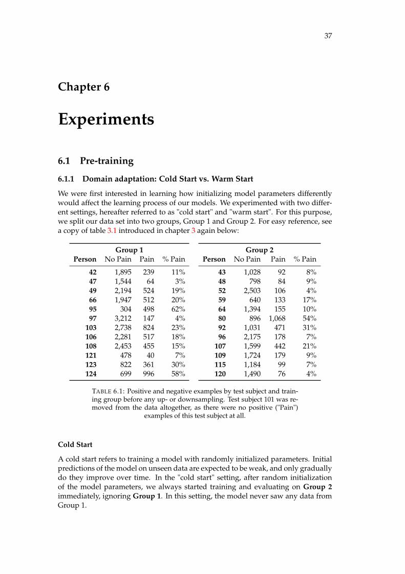
6.1 Positive and negative examples by test subject and training group be-fore any up- or downsampling. Test subject 101 was removed fromthe data altogether, as there were no positive ("Pain") examples of thistest subject at all. . . . . . . . . . . . . . . . . . . . . . . . . . . . . . . . 37

6.2 Balanced training data for experimental setting Randomized Shards . . . 396.3 Number of positive examples by session and test subject. Each test

subject participated in as many consecutive sessions as specified inthe column # of Sessions, starting with session 0. No number indicatesno positive examples for that session (but negative examples, if thesession index is smaller than # of Sessions). . . . . . . . . . . . . . . . . . 41

7.1 Comparison of aggregated results for all learning algorithms in (%).Standard deviation is computed between test subjects. Best resultsper metric are boldfaced. . . . . . . . . . . . . . . . . . . . . . . . . . . . 44

7.2 Acronym Disambiguation . . . . . . . . . . . . . . . . . . . . . . . . . . 457.3 Comparison of aggregated results for all learning algorithms with

centralized pre-training in (%). Standard deviation is computed be-tween test subjects. Best results per metric are boldfaced. . . . . . . . . 45

7.4 Accuracy, Precision-Recall AUC, and F1-Score in (%) by test subject.Best model for each test subject is highlighted in bold. . . . . . . . . . . 49

7.5 Accuracy, Precision-Recall AUC, and F1-Score in (%) by session. Bestmodel for each session is highlighted in bold. . . . . . . . . . . . . . . . 50

7.6 Comparison of model ranking by test subject. Best results per metricare boldfaced. . . . . . . . . . . . . . . . . . . . . . . . . . . . . . . . . . 51

7.7 Comparison of model ranking by session. Best results per metric areboldfaced. . . . . . . . . . . . . . . . . . . . . . . . . . . . . . . . . . . . 52

1

Chapter 1

Introduction

1.1 Motivation

1.1.1 Machine Learning

The not-so-recent-anymore rise of machine learning (ML) models has led to unprece-dented advances in a broad array of fields. In the healthcare space, for example, em-ploying deep learning has shown promise to increase the accuracy of pathologicaldiagnoses[66][33]. In defeating Lee Sedol, widely regarded as the world’s best playerof the traditional Chinese game Go, Google’s AlphaGo computer successfully show-cased that computers powered by deep learning can achieve super-human perfor-mance[55]. Subsequent experiments with an enhanced algorithm dubbed AlphaGoZero that defeated the original algorithm 100-0, and another algorithm defeating hu-man champions in the highly complex real-time computer game StarCraft, helpedfurther publicize the potential power of machine learning algorithms as a whole[56][64]. ML-powered algorithms are also becoming ever more present in our every-day lives, with voice assistants using speech recognition on mobile phones and inthe home[15], and self-driving cars employing computer vision to guide us - mostof the time - safely to our destination[4].

Today’s popularity of machine learning in research and industry can largely beattributed to the unprecedented amounts of data people generate daily using theircomputers, credit cards, and most recently - mobile phones. According to one study,the average smartphone user interacts with his or her device a staggering 2,600 timesper day[69], generating valuable data for advertisers [26], developers [32] and evenmedical researchers [23] with every tap.

1.1.2 Privacy

However, with billions of computing devices generating new data every day, newchallenges and concerns arise. One example is privacy. Large centralized datasetsthat fuel modern ML models present a lucrative target for data breaches. The recentFacebook/Cambridge Analytica scandal has shown the impact that poorly protecteduser data can have [59]. As a consequence, governments have already started to actand passed legislation to protect their citizens, with GDPR in the European Union,the Personal Information Security Specification in China and the definitions of focusedcollection and data minimization proposed by the 2012 White House report on the pri-vacy of consumer data in the United States. As a result, clients ordinarily generatingdata for an ML model might now object to, or be legally prohibited from providingeven anonymized data to a central entity for data processing. Clients may includeindividuals generating data passively through interaction with their devices, as wellas businesses deliberately sharing data with a centralized server for evaluation.

Chapter 1. Introduction 2

Moreover, also the practicality of training ML models on large raw datasets isrunning into constraints. Datasets are continually increasing in size as - in the caseof mobile devices - millions of users generate information every single day. Compil-ing such datasets for evaluation requires a massive infrastructure on the server-sideand strong upload capacity on the client-side. Besides, training a classifier on e.g.,raw image data for a computer-vision algorithm from millions of users in a central-ized location requires exceptionally high processing power, where even the largesttech companies such as Google and Facebook run into limitations.

At the same time, data in most industries is siloed. Owing to industry compe-tition, privacy concerns, and bureaucratic administrative procedures, even data ex-change within the same company is often heavily constrained. As a consequence, anew machine learning technique - federated learning (FL) - is gaining in popularity.First introduced by Google in 2016 [39][28][29], unlike traditional server-side ma-chine learning models FL models are deployed to distributed devices (e.g. mobilephones), and learn locally. Since the training data never leaves the device, feder-ated learning bears great promise for both increased privacy, as well as the distribu-tion of computationally expensive tasks, increasing the training speed of ML modelstrained on large amounts of data.

1.1.3 Healthcare

While the potential applications for federated learning are numerous and highly di-verse, the promise of a privacy-preserving, less computationally hungry machinelearning approach can be particularly valuable for the healthcare space. Healthcarepatient data are typically among the most strictly regulated with HIPAA[52] in theUS and GDPR[16] in the European Union governing the rules by which such datacan be accessed. At the same time, pooling healthcare data from healthcare facili-ties, insurance providers, and government agencies on a regional, national or evenglobal scale holds enormous potential for example for rare diseases research[67] ortreatment best-practices.

Pain

One example, where hospitals could work together to improve the lives of the pa-tients they treat is the identification of pain. Detecting pain in patients to provideeffective treatment is a critical job that hospital staff needs to perform on an on-going basis, and the automation of this task has been of interest to researchers forquite some time [2][36][35]. Shortcomings so far, among other things, have includeda lack of labeled training data for machine learning classifiers. If different hospi-tals, senior-care facilities, and other healthcare institutions collaborated in training ashared model for this task, the amount of available data would increase significantly,likely improving the performance of any classifying algorithm, in the process.

In "RoboChain: A Secure Data-Sharing Framework for Human-Robot Interac-tion" [10] the authors propose a framework to jointly learn a machine learning modelon private, local data, building upon the latest advances in blockchain technology,and federated machine learning. Building on their work, this thesis further dis-cusses the potential of federated learning in general, and as a catalyst for futurebreakthroughs in the medical space.


1.2 Contributions

Our work contributes to the field of pain study by way of monitoring Facial ActionUnits, as well as to the field of federated machine learning, by introducing a novelalgorithm we dub federated personalization. More specifically, we:

1. Show that a lightweight CNN architecture can learn to recognize pain from thefacial expressions of individuals.Based on a data set labeled according to the standard of the "Facial ActionCoding System" introduced in chapter 3 we successfully train a convolutionalneural network to predict when a person is in pain, using a video stream ofthat person’s face as an input.

2. Show that the federated learning algorithm is robust even in a "production-level" setting, learning a challenging data set that changes over time.Many papers discuss the benefits of federated learning in benchmarking per-formance on toy-data sets such as MNIST or CIFAR-10[39][12]. In our case, weexperimented with a highly unbalanced dataset, where positive and negativeexamples are not easily distinguishable. In our experiments, the underlyingdata distribution also evolves, as would be expected if we put the model intodeployment.

3. Introduce a new federated learning algorithm that adds additional privacypreservation, at only a modest expense of performance.Our "federated personalization" algorithm only shares some layers with thecentral server, but not all, which makes it harder for an adversary to learn pre-viously unknown information about an "honest" client participating in jointlylearning a model. While these "global" layers are still averaged between par-ticipants, the "local" layers only continue training on each client’s local dataset.

4. Provide specific directions for future research.We suggest a more sophisticated validation-set algorithm that leverages moreprecise early-stopping for a sparse data set such as the pain data set. We alsorecommend implementing a "fallback"-model in a federated setting that kicksin if an updated global model would likely worsen the performance of a givenclient.

1.3 Outcomes

We evaluated 24 different test subjects experiencing pain, split into two groups (group1 and group 2). Group 1 was used to pre-train a model that we used as a baseline.Group 2 was used to continue training on the pre-trained model and evaluate modelperformance. Table 1.1 shows a summary of our key findings. The table comparesthe following methods for classifying the pain data set introduced in chapter 3:

RANDOM: A CNN where weights have been randomly initialized using the glo-rot uniform distribution [13].

BC-CNN: The Baseline Centralized CNN, a model that was pre-trained on the 12test subjects of group 1.


Weighted AVG + STDExperiment ACC PR-AUC F1

RANDOM 43 ± 14 30 ± 15 31 ± 2BC-CNN 72 ± 12 54 ± 23 47 ± 24C-CNN (C) 75 ± 13 57 ± 21 49 ± 21F-CNN (C) 74 ± 11 59 ± 23 51 ± 25FP-CNN (C) 76 ± 12 56 ± 21 49 ± 23FL-CNN (C) 75 ± 13 54 ± 20 47 ± 23

TABLE 1.1: Comparison of aggregated results on group 2 data for alllearning algorithms with centralized pre-training in (%). Standard

deviation is computed between test subjects.

C-CNN (C): The Centralized CNN with Centralized pre-training, a model that wasinitialized with the weights of the BC-CNN and trained with centralized learningand vanilla SGD.

F-CNN (C): The Federated CNN with Centralized pre-training, a model that wasinitialized with the weights of the BC-CNN and trained with federated leraning.

FP-CNN (C): The Federated, personalized CNN with Centralized pre-training, amodel that was initialized with the weights of the BC-CNN and trained on the fed-erated personalized learning algorithm, introduced in chapter 5.

FL-CNN (C): The Federated, local learning CNN with Centralized pre-training, 12individual models (one for each client), each initialized with the weights of the BC-CNN and trained separately, with the performance averaged across models.

As we can see from this table, the baseline for accuracy is beaten by every learn-ing algorithm. When looking at PR-AUC and F1, both measures for identifying howwell the model identifies positive examples, we find that FL-CNN (C) struggles tobeat the baseline, while all other learning algorithms manage to outperform it. F-CNN (C) performs the best, followed by C-CNN (C) and FP-CNN (C), and finally,FL-CNN (C).

1.4 Outline

See the following for an outline of the remainder of this thesis:

Chapter 2: Background and related work This chapter introduces the necessarymachine learning preliminaries that this thesis builds on. It explores neural net-works in general, their strengths and weaknesses, convolutional neural networks,and finally, the federated learning algorithm.

Chapter 3: Data In this chapter we take a deep-dive into the data, and discuss thechallenges the data set presented, as well as the techniques we used to augment thedata and tackle these challenges.


Chapter 4: Model Architecture In this chapter, we present the underlying modelarchitecture we used to assess our different learning algorithms. We show the origi-nal model architecture we started experimenting with as well as the final architecturethat produced the best results. We also comment on the general viability of com-monly employed model architectures for image recognition tasks such as ResNet50and VGG19.

Chapter 5: Experiments This chapter discusses the different learning algorithmswe tested, as well as the experimental settings we designed. It also introduces anovel algorithm we dub "federated personalized learning" that we designed for ad-ditional privacy protection.

Chapter 6: Results & Evaluation In this chapter we discuss the results that thedifferent learning algorithms achieve, and analyze the absolute performance of eachalgorithm as well as their relative performance to each other.

Chapter 7: Conclusions & Future Work In the final chapter, we conclude our workand point to directions that future research can take. Expressly, we point towardspossible advancements of our validation algorithm, as well as the federated person-alized learning algorithm.

6

Chapter 2

Supervised machine learning

2.1 Machine Learning Preliminaries

Machine learning tasks can generally be grouped into two different paradigms: Su-pervised and Unsupervised Learning. In unsupervised learning, a typically unlabeleddata set is fed to an algorithm, which is designed to detect previously unknownpatterns in the data. Clustering algorithms such as K-Nearest Neighbor, or GaussianMixture Models[47] are examples of unsupervised learning, where unlabeled data isbeing grouped based on some shared properties. With supervised learning, on theother hand, labeled training data fed to an algorithm to learn a function that canmap an input X to an output Y. Such a function can serve to solve a classification task(e.g., does an image contain a red car or a blue bus), or a regression task where a con-tinuous variable is predicted (e.g., given X liters of gasoline, we expect a car to beable to drive for Y kilometers). The federated learning algorithm (described in detailin section 2.2) advances the field of supervised learning, as it allows multiple clientsto jointly learn such a function. In the following, we will thus focus on supervisedlearning.

2.1.1 Multilayer Perceptron

While determining the amount of gasoline required to travel a certain distance couldpotentially be solved with a simple linear regression model, image classificationtasks such as the one mentioned above typically require more sophisticated mod-els. This has led to the increasing popularity of artificial neural networks (ANNs).Due to the typically much larger number of tunable parameters, ANNs can approxi-mate significantly more difficult functions, qualifying them well for non-linear taskssuch as speech recognition or object detection.

Multilayer perceptrons (MLP) are a type of feedforward ANN. The perceptronwas first proposed by Rosenblatt in 1957 [49]. A multilayer perceptron consists ofone input layer x, one to many to hidden layers hi and an output layer y. For simplic-ity, we will assume a variant of the MLP, the single-layer perceptron in the following.Figure 2.1 shows an example of such an architecture. When training the MLP, wefeed a sample of our training data to the input layer, where each neuron representsa feature (e.g., one pixel of an image, or one column labeled "age" of a table con-taining user-data). Each of the input layer (an n-dimensional vector where x ε Rn)is connected to each neuron of the first hidden layer hi (an m-dimensional vectorwhere hi ε Rm), which is again connected to the output layer y, a k-dimensional vec-tor y ε Rk, where k is the number of classes the perceptron is designed to predict.In a binary case, one neuron (instead of 2) is enough, as that neuron could outputa value closer to 0 for class one and a value closer to 1 for class two. The neurons

Chapter 2. Supervised machine learning 7

are connected by typically randomly initialized weights w ε Rm for the input layerto the hidden layer and w ε Rk to the output layer.

FIGURE 2.1: Multi-layer perceptron

Neuron

As the name suggests, neural networks such as the MLP are made up of many inter-connected neurons. In the "forward-pass", i.e. when the network is asked to makea prediction based on some given input, neurons receive n inputs, which are mul-tiplied by a corresponding weight, and summed up to get a pre-activation value z,which is then passed to the activation function f , which typically performs a non-linear transformation on the value (explained more in detail below). This is shownin figure 2.2 and can be summarized as:

y = f (z) = f (∑i

wixi) = f (wTx) (2.1)

Activation Function

Activation functions are required to introduce non-linearity to an ANN. If we con-structed an ANN without activation functions we would simply be chaining a num-ber of linear neurons of the form y = wTx, the result of which would just be another

FIGURE 2.2: An exemplary neuron in a neural network


linear function. As discussed at the beginning of section 2.1, this would be inade-quate for many applications. Some of the most popular activation functions are:

Linear (identity) Does not transform x.

identity(x) = x (2.2)

Sigmoid Compresses the output to the range between 0 and 1. Often used in theoutput layer for binary classification tasks[43].

sigmoid(x) =1

1 + (e−x)(2.3)

Tanh Adjusts sigmoid such that it ranges between -1 and 1[43].

tanh(x) =2

1 + (e−2x)− 1 (2.4)

ReLU Short for "Rectified linear unit". A piece-wise linear function returning x ifx is larger than 0, else returns 0[43].

relu(x) ={

x if x > 00 otherwise

(2.5)

Softmax n-dimensional sigmoid, compressing the sum of the output vector to 1,often used in the output layer for multi-class classification tasks[43].

so f tmax(zi) =ezi

∑k ezk; z ε Rn (2.6)

Loss Function

During the training of the network, once the forward-pass is complete and the net-work produced some numerical result, this result is then compared to the actual,known labels, and the error is calculated. For example, in a multi-class classificationtask where the model needs to differentiate between cars, planes, and trains, themodel might produce an output vector yielding probabilities of [0.5, 0.2, 0.3] for asingle image. Assuming the image shows a car, the corresponding one-hot encodedvector will be [1, 0, 0]. These vectors are then passed into a Loss Function, which cal-culates the prediction error, which is used to update the model weights connectingthe model’s neurons, in a subsequent step discussed in the next paragraph. Com-mon loss functions are:

Binary Crossentropy This is typically used for binary classification tasks[25].

l(y, y) = − 1N

N

∑i=0

(y× log(yi) + (1− y)× log(1− yi)) (2.7)


Categorical Crossentropy Similar to binary cross-entropy but N > 2, used for multi-class classification tasks[25].

L(y, y) = −M

∑j=0

N

∑i=0

(yij × log(yij) (2.8)

Mean Squared Error Typically used for regession tasks as it computes the eu-clidean distances between the prediction vector and the labels vector[25].

L(y, y) =1N

N

∑i0

(yi − yi)2 (2.9)

Gradient Descent

In order to learn a model that can make accurate predictions, we aim to minimizethe loss of the model by adjusting our model’s parameters (or weights). While thisis generally done by optimizing them for the training data, the model is also oftenvalidated on otherwise unused data. In the end, the parameters with the best per-formance on the validation set are selected.

For minimizing L a large part of machine learning research is dedicated to alearning algorithm called gradient descent[5].

In gradient descent, we iteratively adjust the model parameters such that in eachiteration the value computed by the loss function is brought closer to a local or globalminimum. An illustration of this technique can be found in figure 2.3, where theloss (indicated by the arrows) is gradually improved by updating two parameters.Starting with randomly initialized parameters, we compute the partial derivatives

FIGURE 2.3: A two-dimensional illustration of gradient descent

of the loss function with respect to the model parameters and store the result in agradient. The gradient is an indication of the slope of the loss function given thecurrent values of our parameters, as well as the direction in which the parametersshould be updated. After each parameter wi is updated, this process is repeated,until a local or global minimum of the function we are trying to approximate isfound. Formally these steps can be defined as:

wi ← wi − η × ∂L∂wi

, (2.10)


where η represents the algorithm’s "learning rate", discussed more in-depth below.In practice, one of two variants of gradient descent is usually used. In StochasticGradient Descent, one data point is used to update the weights of the model, whilein Mini-batch gradient descent small batches of data points are used instead of thewhole data set. These variants are applied since having to iterate through the entiredata set for each step of gradient descent would be too computationally expensive.SGD works under the assumption that much of training data is similar, and thus ∇Lcan be called an unbiased estimator of∇L. This property implies that while individ-ual estimates on a batch might be inaccurate, the randomness will average out overtime and the parameters are updated in the correct direction.

Finally, we need to mention that with gradient descent, we can only guaran-tee that the model converges to a local optimum. As there are generally few localoptima in high-dimensional spaces, this is seldom a problem in real-world applica-tions. However, gradient descent can get stuck on a saddle point or a plateau, whichoccurs more frequently[7]. While on a saddle point the gradient might be zero in alldirections, there may still be a better point somewhere in the vicinity. See figure 2.4for an example.

FIGURE 2.4: The stochastic gradient descent algorithm finding a localoptimum

Computational Graph

As eluded to above, the gradient descent algorithm requires calculating partial deriva-tives. While derivatives for simpler methods like linear or logistic regression arewell described in the literature, deriving the gradient for more complex functionsbecomes increasingly difficult. For a neural network with many layers and evenmore neurons, setting up a long function that describes the entire network is nearlyimpossible.

Computational graphs represent an abstraction that allows machine learning re-searchers to circumvent this problem. In place of attempting to construct a functionalrepresentation of an entire neural network, of which a derivative can be computed,the network is broken down into smaller more manageable pieces, such as multi-plication or the exponential function, where the direct derivative is known. Thesesmaller functions are connected into a graph where each node represents a function,and each edge shows how information moves between nodes. An example of this isshown in figure 2.5.


FIGURE 2.5: A computational graph of the function f (x, y)

This graph represents the function

f (x, y) = x×√y +√

y. (2.11)

It also shows how constructing a graph can be more computationally efficient asthe term

√y only needs to be calculated once. Representing our model as a graph

allows us to employ back-propagation, an algorithm that applies the chain rule ofderivation to find the partial derivative of the loss function with respect to the modelweights. For the last layer in the model before the output layer, this partial derivativecan be described as:

∂L∂W(L)

=∂L

∂A(L)× ∂A(L)

∂Z(L)× ∂Z(L)

∂W(L), (2.12)

where L describes the loss, W the weights, A the activation value and Z the pre-activation output. For additional layers, we need to add to this function by multi-plying it with the partial derivatives of the weights of those layers with respect tothe loss.

Overfitting

Overfitting is a common problem with training neural networks[6]. A neural net-work is an eager learner, meaning that it stores many parameters that were optimizedon an underlying training data set. Overfitting refers to the processes of learning par-ticular pieces of information about the training data, which do not generalize wellto the overall population. The result is typically a model that yields a low loss whenevaluated on the training data itself, but a much higher loss when evaluated on un-seen test data. An example can be seen in figure 2.6, where the grey line representsa model that overfit on a specific set of features and maps the training data distri-bution very closely whereas the model represented by the green line was trained tolearn more general features.

The opposite problem is "underfitting" when the model is not strong enough tocapture discriminative information on the training data and yields a high trainingand test loss. While this can often be addressed by increasing the number of learn-able parameters in the network and training the model for longer on the trainingdata, overfitting is more challenging to tackle.

Early Stopping

Neural Networks tend to overfit on the training data when they train on it for toomany iterations (also referred to as "epochs"). To address overfitting, we can applyearly stopping[3]. With early stopping, we split the training data into a trainingset and a validation set. After each epoch (a full pass over the training data), thequality of the model is evaluated on the validation set. If the validation loss does


FIGURE 2.6: An example of overfitting. The grey line represents amodel that overfits, whereas the green line represents a model that

learnt more general features of the population.

not improve within a specified number of epochs, training is stopped. Typically, themodel weights that yielded the lowest validation loss are then restored at this point.

Regularization Techniques

Dropout Dropout is a regularization technique, whereby each neuron except theoutput neurons has a probability p of being ignored during a given training step[60].During the forward- and backward-pass during this training step, the neuron is shutoff and does not perform any calculations. As a result, the neural network tends toconverge slower, but inter-dependency between neurons across layers is reduced,allowing the model to generalize better on unseen data. We can see in figure 2.7 howthis process looks in practice. Dropout is only applied during the training stage. At

FIGURE 2.7: An example of dropout for two consecutive trainingsteps

prediction time, all neurons are active; however, their weights and activations aretypically scaled to the dropout factor as otherwise, the input that a neuron receivesduring prediction time would on average be 1

p higher than during training time.

L1 and L2-Regularization L-Regularization combats the issue of model weightsgrowing out of proportion[41]. In both techniques, the objective function is modifiedby adding the model weights to the model loss. In this case, the model Ois penalizedif it achieves a low loss at the cost of large weights. Thus, in order to reduce theloss, the weights need to be kept small as well. With L1-regularization, the absolutevalue of the weight is added to the objective function. The parameter λ indicates


how much the model should be regularized.

J(W) = L(Y, A) + λ ∑w|w| (2.13)

This means that for the update rule in the backward pass, a fixed movement towards0 is considered.

w← w− η(∂L∂w

+ λsign(w)) (2.14)

For L2-regularization, the squared weight w2 is added to the objective function along-side the loss.

J(W) = L(Y, A) + λ ∑w

w2 (2.15)

The update rule shows that in L2-regularization the update is now proportional tothe weight itself, indicating that large weights shrink proportionally faster.

w← w− η(∂L∂w

+ 2λw) (2.16)

The L1 regularizer tends to produce sparse weights, as most weights are pushed to0, and consequently only the most useful weights will be non-zero to make predic-tions. As a result of this sparsity, feature selection occurs, where L1 regularisationforces each layer to select only a few inputs in order to keep the weights small. Bycontrast, with L2 regularization, layers benefit from taking in a combination of fea-tures, as weights are not pushed as strongly towards 0 when they already have smallvalues.

Batch normalization Batch Normalization is a normalization technique intro-duced in 2015 by Sergey Ioffe and Christian Szegedy in their paper ’Batch Normaliza-tion: Accelerating Deep Network Training by Reducing Internal Covariate Shift’[42] andtoday it is used in almost all convolutional neural network architectures (see sec-tion 2.1.2). According to the original paper, batch normalization helps reduce theinternal covariate shift of the hidden layers of the network. However, in a more re-cent paper titled "How Does Batch Normalization Help Optimization?"[51], the authorssuggest that batch normalization actually "makes the optimization landscape signif-icantly smoother." The result is a changed behavior of the gradients, which becomesmore predictive and stable.

Historically, research has focused on uniformly distributing the data fed into theinput layer of the neural network. For example, in a case where the model is trainedto separate cats from dogs, it makes intuitive sense to feed cats and dogs of all shapesand colors to the model in a given minibatch during training, rather than feedingblack cats and dogs in one mini-batch to the model and brown cats and dogs in thenext because these subsets of data have different distributions.

For the hidden layers, however, this input distribution changes every time thereis a parameter update in the previous layer. This challenge is addressed by batchnormalization. BN replaces the incoming vector of pre-activation values of a givenminibatch in a given layer with its normalized version. Formally this process canbe summarized in four steps (simplified for one layer to limit the number of super-scripts):


1. Calculate the mean µ of the mini-batch.

µ =1m ∑

iz(i) (2.17)

2. Calculate the variance σ2 of the mini-batch.

σ2 =1m ∑

i(z(i) − µ)2 (2.18)

3. Calculate the normalized value of z, znorm.

z(i)norm =z(i) − µ√

σ2(2.19)

4. Calculate znorm by multiplying znorm with a scale γ and adding a shift β andreplace the pre-activation z with znorm.

z(i)norm = γz(i)norm + β (2.20)

Throughout the experiments conducted in light of this thesis, we experimentedwith all of the regularization techniques mentioned above and found batch-normalizationto be the most effective.

2.1.2 Convolutional Neural Networks

Convolutional Neural Networks are another type of feedforward neural network,typically used for image recognition/computer vision tasks in deep learning[30].The purpose of employing convolutional layers is to learn useful features from aninput image such as edges (horizontal, vertical, or diagonal) and spatial relation-ships between elements in an image (a face usually consists of eyes, a nose, ears, anda mouth). This is done through applying one or more filters to the input image (andin the case of further hidden convolutional layers applying additional filters on theoutputs from the first convolutional layer).

Filters

In image processing, a filter refers to an operation that transforms an image in ameaningful way, i.e., by increasing the image’s contrast or grey-scaling an RGB im-age. This is done by applying a standard, predefined mathematical operation oneach pixel or a group of pixels. To grey-scale an image, for example, a filter wouldmultiply each pixels’ image channels (Red, Green, and Blue) by 1

3 and sum the re-sults to output a single channel that held the numerical average of the three colorchannels. In this example, the filter is a fixed 3-dimensional vector of shape (1 x 1 x3), with each dimension holding the value 1

3 . See figure 2.8 for a pictorial descriptionof this process.

In convolutional NNs, rather than specifying a filter’s values in advance, thefilter’s values are randomly initialized and then learned over consecutive trainingiterations. While the last dimension of the filter (the depth, or number of kernels) willalways need to equal the last dimension of the input shape, the height and width ofthe filter are hyperparameters that can be freely tuned.


FIGURE 2.8: Example of applying a filter consecutively to each pixelof an image to greyscale the image

Usually, a convolutional layer holds more than one filter, each of which learns aseparate feature of the input image (e.g., filter 1 learns horizontal edges, while filter 2learns round edges. All learned features are subsequently combined in the forwardpass to make a prediction.

Kernel

One filter is typically made up of several kernels. The term kernel refers to a 2D arrayof weights, which are the parameters that are being tuned in a convolutional layer.See figure 2.9 for an example. Here the filter is a (3 x 3 x 3) matrix, meaning that itconsists of 3 kernels of the shape (3 x 3). First, each kernel is applied to one inputchannel, without padding (explained below). The three convolutions that are per-formed result in three channels, each with a size of (3 x 3). These resulting channelsare then summed together, forming one single channel with dimensions (3 x 3 x 1),which is the result of the convolution.

FIGURE 2.9: An example of a filter consisting of three kernels slidingthrough an RGB image translating it into one output channel

Convolution

We can describe a convolution as follows:

S(i, j) = (K ∗ I)(i, j) = ∑m

∑n

I(i−m, j− n)K(m, n) (2.21)

The function above describes the process of taking a two-dimensional input imageI as an input, and applying a two-dimensional kernel K on the image. The kernel is


applied to a region of the image that matches its shape. Then, an element-wise sum-product is calculated. The kernel is then moved by a predefined number of steps(called stride), and the operation is repeated. Applying this algorithm has the sameeffect as multiplying the input image by a sparse matrix.

Padding

As can be seen in figure 2.9 a filter with kernels of dimensions larger than (1 x 1) re-duces the size of the input image. If this is not desired, it can be prevented by addingsome padding (pixels with 0 values) around the input image, as seen in figure 2.10.

FIGURE 2.10: Example of padding, where a (2x2) kernel and a (4x4)input image (green) produce a (4x4) output image (blue)

Pooling

Still, with images larger than 100 x 100 pixels padding only has a negligible impacton the size of the output. If a reduction in the height and width of the input channelsis desired, we can apply a pooling mechanism, which computes a summary statisticof a group of adjacent pixels. One of the most common techniques is called max-pooling. In max-pooling, a pool-size (height and width) is defined, which is thenapplied to the output of the convolutional layer. The max-pooling layer selects thehighest activation value from its pool, which then becomes part of the output matrix.See figure 2.11. Pooling generally makes the network more translation invariant,

FIGURE 2.11: An example of max-pooling with a 2x2 pool-size. Onlythe highest activation value in a given 2-by-2 quadrant is added to

the output.


meaning that a slight rotation or shift in the image will not substantially alter themodel’s prediction.

Parameter Sharing

One final reason why convolutional networks have become increasingly popular formany deep learning tasks is parameter sharing. In a traditional multilayer percep-tron as discussed in section 2.1.1 every weight in the model is used exactly once,when the output of a layer is computed, by multiplying it with one element of theinput. In a convolutional neural net, each member of the kernel (see above), is usedat every input position, except for the boundary pixels, if no padding is used. Thishas no impact on the forward propagation run-time, but drastically reduces the spa-tial requirements of the model as significantly fewer parameters need to be stored.Also, convolution is dramatically more memory efficient than dense matrix multi-plication as a result.

2.1.3 Transfer Learning and Domain Adaptation

As mentioned in section 2.1.1, the parameters of a neural network are typically ini-tialized to random values, when learning a new task. Translating random initializa-tion to how humans learn would imply completely resetting the brain each time welearned a new task. Humans, however, have the innate ability to transfer knowledgeabout one domain to another related domain. For example, pre-existing knowledgeabout how to ride a bike can help when learning how to ride a motorcycle.

Transfer Learning

In deep learning, the idea of applying pre-existing knowledge learned for a specifictask on one data distribution to a new task on another data distribution is referredto as transfer learning. In computer vision, for example, if the task is to identifycars in images, initializing a model with the parameters of another model originallydesigned to recognize trucks, can speed up training significantly over alternativelyinitializing parameters completely randomly. The reasoning behind this approach isthat in computer vision tasks, as discussed in the previous section, objects in imagesshare low-level features, extracted by the lower levels of the neural network. Theupper layers, - often dense, fully-connected layers - take these extracted features in,and learn the actual classification task.

Popular deep learning libraries such as Tensorflow and PyTorch allow users viaan API to download popular deep learning architectures such as ResNet50[19] orVGGNet[57]. Rather than randomly initializing and training these architecturesfrom scratch, which due to the many millions of trainable parameters would becost-prohibitive and results in long training times, they can be initialized with pa-rameters learned on the Imagenet data set, a dataset containing images of 1,000 dif-ferent objects[50]. Due to the diversity of the Imagenet data set, these trained modelparameters have been shown to serve as a good starting point for another com-puter vision task, underscoring the viability of transfer learning[54]. In practice, asthe upper layers are typically fine-tuned for a specific classification task, they arecommonly replaced with randomly initialized layers, when a new task is to be per-formed. To train the new final layers, the lower, convolutional layers are typically"frozen", meaning that their parameters do not change during training so that the


low-level features learned on the Imagenet data set are preserved. Only the finallayers are then freely trained to learn the new classification task.

In transfer learning, however, we are still assuming that our initial training setdistribution is representative of the underlying distribution. I.e., if we initializeda model architecture such as VGGNet on the trained parameters of the Imagenetdataset and subsequently trained the final layers to recognize taxi cabs in New YorkCity, we would expect the model also to recognize taxi cabs in Berlin. However,while the model might still perform better than the original VGGNet architecturedue to some similarity between New York and Berlin taxi cabs, it would likely stillnot perform as well as expected. The reason is that the problem domain changed. Inthis particular case, the domain of the input data changed, while the label’s domain(the task domain) stayed the same. Enter domain adaptation.

Domain Adaptation

Domain adaptation can be considered a sub-field of transfer learning and is em-ployed when a model trained on a source distribution is put into practice in thecontext of a different (but related) target distribution [14]. Generally speaking, thelevel of relatedness between the source and the target domain determines how suc-cessful the domain adaptation will be. Returning to the example of taxi cabs in NewYork and Berlin, the next step would require to continue training the modified VG-GNet model, which has already been trained on images of New York taxi cabs. Twomethods are typically used for continued training: Reweighing the source samples,which would imply training only on Berlin taxi cabs, or learning a shared spacebetween the distributions, i.e., training on a joint data set of New York and Berlincabs. Either approach, however, would likely decrease training time and yield bet-ter results faster, compared to randomly initializing the final layers of the originalVGGNet architecture again and training them from scratch.

2.2 Federated Machine Learning

2.2.1 Overview

Federated Machine Learning was first introduced by Google in 2016 [39][28][29].Different from a centralized setting, in a federated learning setting, multiple devicese.g., end-user devices such as mobile phones, or business infrastructure such as hos-pital servers, contribute to learning a machine learning classifier. The classifier canbe a deep neural network, but also a simpler model, with fewer parameters suchas a support vector machine, or a logistic regression model[17]. Federated learn-ing models are distinct in that the original training data never leaves the respectivelocal device that collected it. Each device (also dubbed client) maintains a versionof the same model, which is updated with every new observation. The updates tothe model (e.g., the updated weights and bias of neurons in a neural network), notthe observations themselves, are then shared with a central server, which averagesthe new models from all participating devices. Once a new version of the model hasbeen trained, it is pushed back down to all clients. This process repeats continuouslyuntil the model converges.

Figure 2.12 displays a graphical representation of this process. In (A) the server-side model is pushed down to a mobile phone, which subsequently trains the modelon local data. Training happens on several devices, as depicted in (B). Subsequently,


the new models are pushed to the cloud (the central server), and averaged, to arriveat the model in (C). This model is then pushed to all devices, and the process startsagain.

FIGURE 2.12: Federated Machine Learning: Conceptual Architec-ture[37]

Three primary benefits emerge from this approach, the first of which will bediscussed more in-depth in the remainder of this work:

Privacy: In an FL approach, the central server only aggregates ephemeral parame-ter updates, meaning model updates that last only long enough to be transmitted tothe central server and incorporated into the central model. This implies that clientsstill need to trust the entity aggregating different models enough to receive the in-dividual parameter deltas, but clients only receive the final trained model for infer-ence. As a result, the attack surface for gaining access to personal data is limited tothe device only, as opposed to the device and the cloud.

Computing power: Shifting computation down to the devices also significantlyreduces the processing power required in a central location, since the role of thecentral entity is merely to average the updates from all participating devices, as op-posed to continuously retraining a global model on new sets of data. Today’s mobiledevices are becoming increasingly powerful, especially with the emergence of AIchipsets[24]. Thus, considering that there are billions of mobile devices worldwide,the accumulated computing power from these devices far-surpasses that of even themost potent datacenter.

Real-time learning: Finally, since the models are trained locally, updates are in-stant, enhancing time-to-prediction, and as a consequence, user-experience. More-over, typical implementations to date have ensured that model updates are onlypushed to and pulled from a central server once a device was idle, plugged intopower and connected to a WiFi connection. Limiting updates to such a setting ad-dresses the issue of unstable internet connections and ensuring that user-experienceis not affected detrimentally due to power-consuming up- and download processes.[70].


2.2.2 The Federated Averaging Algorithm

As discussed above, in federated learning, we assume that our data is not centrallystored, but partitioned over K number of clients. Assume that

• Each partition can be represented as a set of indices Pk of data points that agiven client k holds

• n represents the number of all data points collected by all clients and thus nkrepresents the number of data points that the client holds

• nk = |Pk|

If the standard definition of minimizing a loss function is given by

minθ∈Rd

f (θ) (2.22)

where

f (θ)de f=

1n

n

∑i=1

fi(θ) (2.23)

and fi(θ) represents the loss for a prediction of one observation (xi, yi given modelparameters θ, this loss function can be rewritten to represent K clients in a federatedsetting, such that

f (θ) =K

∑k=1

nk

nFk(θ) (2.24)

whereFk(θ) =

1nk

∑i∈Pk

fi(θ) (2.25)

.

To break this down: Instead of computing our average loss (e.g. our MSE) asan average over n number of samples from a centralized data set as 1

n ∑ni=1 fi(θ),

we compute the average loss Fk(θ) for a specified client k as 1nk

∑i∈Pkfi(θ) and then

group the loss of all participating clients K, by computing a weighted average lossbased on the number of data points nk that each client holds.

Analog to computing the loss, we also compute the gradients of the federatedmodel. Keeping equation (2.10) in mind, in a federated setting each client computesthe average gradient gk on its local data as

gk = ∇Fk(θ) . (2.26)

Then, each client takes a step of gradient descent and updates its parameters accord-ingly, formalized as

∀k, θk ← θ − ηgk . (2.27)

This step can be repeated multiple times, i.e., for multiple epochs E, until a cen-tral server then computes the weighted average of these gradients similar to theweighted average of the loss above as

θ ←K

∑k=1

nk

nθk (2.28)


to update the model parameters of the overall model, stored on the central server.This concludes a full round of updates to the global model.

Assuming mini-batch stochastic gradient descent, in such a federated setting thecomputational effort for one full update is controlled by three parameters:

1. The fraction C of clients K that participate in a given update round.

2. The number of steps of gradient descent (or epochs) E that each client performs

3. The batch size B used for all client updates

While C impacts the computational power required at the server level (more par-ticipating clients requires more transfer of data to the server and more effort in ag-gregating information), E and B impact the computational effort required on theclient-side. The complete pseudo-code for this approach was first proposed by [39]and is provided for convenience in Algorithm 1.

Algorithm 1 FederatedAveraging. The K clients are indexed by k; B is the localminibatch size, E is the number of local epochs, and η is the learning rate. w denotesthe model parameters.

procedure SERVER EXECUTES:initialize w0for each round t = 1, 2, ... do

m←max(C× K, 1)St ← (random set of m clients)for each client k ∈ St in parallel do

wkt+1 ← CLIENTUPDATE(k, wt)

wt+1 ← ∑Kk=1

nkn wk

t+1

procedure CLIENTUPDATE(k, w) . Run on client kB ← (split Pk into batches of size B)for each local epoch i from 1 to E do

w← w− η∇`(w; b)return w to server

2.2.3 Applications for Federated Learning

Potential applications for federated learning are vast and differ substantially in ver-tical and specific use-case, but typically bear three common traits[70]:

1. Task labels do not necessarily need to be provided by humans but can be de-rived naturally from user interaction.

2. Training data is privacy sensitive

3. Training data is large, and is difficult to be feasibly collected in a central loca-tion

Not all of these conditions strictly need to hold when applying federated learning,but it is under these circumstances, that federated learning provides the most sig-nificant value over other machine learning techniques. To illustrate the potential offederated learning, in the following, we briefly review some of the recent applica-tions of FL models in practice.


Brain Tumor Segmentation Without Sharing Patient Data Computer chip-makerintel [53] leverages FL to showcase how multiple healthcare institutions can collab-orate in a privacy-preserving manner, leveraging each institution’s electronic healthrecords (EHR). The authors argue that while collaboration between institutions couldaddress the challenge of acquiring sufficient data to train machine learning clas-sifiers, but the sharing of medical data is heavily regulated and restricted. Theypresent the first use of an FL classifier for multi-institutional collaboration and findthat they can learn a similarly performant federated semantic segmentation model(Dice=0.852) compared to that of a model trained on centralized data (Dice=0.862).This strengthens the hypothesis that FL can lead to breakthroughs in the medicalspace without compromising patient privacy.

Improving Firefox Search Bar Results In [18], the author leverages federated learn-ing in a production level setting using data from 360,000 users to improve the searchresults in the Firefox Search Bar, without collecting the users’ actual data. Millionsof URLs are entered into Firefox daily, thus notably improving the auto-completefeature for users enhances user experiences and can increase customer retention.

Improving Google Keyboard Suggestions Google describes one of the first im-plementations of federated learning on a large scale, training a global model to "toimprove virtual keyboard search suggestion quality"[70]. In their paper, they ad-dress many of the technical challenges of coordinating training on millions of de-vices worldwide. Examples include connectivity issues, the bias of training a modelacross different time zones, and minimizing the impact on user experience that train-ing a machine learning model locally has (e.g., battery-life and device-speed). Theynote that future work on privacy still needs to be done and cautiously call theirmethod "privacy-advantaged", vs. "privacy-preserving".

2.2.4 Practical Challenges for Federated Learning

Federated Learning is not without its challenges. A few key-properties describe atypical federated optimization problem:

Non-IID A dataset’s data points are said to be IID if they are independent andidentically distributed. If the IID assumption holds, the underlying mathematicaland statistical techniques can often be simplified. For example, if we draw a suffi-ciently large sample at random from the overall distribution, we can with a specifiedlevel of confidence state that the sample is representative of the overall population.In Federated Learning, clients’ datasets will often differ substantially from those ofother clients (e.g., in the case of mobile phones the phone’s dataset is dependentmostly on the interaction with one particular user). Thus, sampling a client at ran-dom will likely not yield a dataset that is representative of the global population dis-tribution. Other sampling techniques, such as stratified sampling, can be employed tomitigate this problem.

Unbalanced In a similar fashion, clients’ datasets may vary substantially in size.Again using the example of mobile phones, some people may use their phones sig-nificantly more than others, creating larger datasets that potentially skew the result-ing weighted average in their direction, while penalizing users generating less data.


Limited Communication Mobile phones are frequently offline or are connected toflaky or expensive internet connections. Healthcare facilities, especially in rural ar-eas in the United States, often have only slow internet connections [38] or a minimalnumber of computers that are linked to the internet. While it is usually cheap tocompute updates locally, since the amount of training data is low, communicatingthese results becomes much more time-consuming, making communication-speedand averaging the bottleneck in federated learning.

Maintaing performance Finally, and perhaps most importantly, since a global fed-erated model is not trained on the raw data, but rather a proxy (the clients’ pa-rameters), and only local models have access to this data, care needs to be takenin achieving similar performance in a federated setting compared to a centralizedmachine learning approach. If a model fully preserves the privacy of a client butproduces inaccurate predictions, it can essentially be rendered useless.

In the remainder of this work, we will focus on the issues of handling non-IIDand unbalanced data, as well as maintaining performance, while leaving the issue oflimited communication to future work.

24

Chapter 3

Data

3.1 Overview

As eluded to in chapter 2 one of the most promising applications of federated learn-ing is the healthcare space, where many different entities can jointly learn a modelwithout sharing sensitive raw data, thereby adhering by privacy regulation such asGDPR in the EU or HIPAA in the US.

To demonstrate the effectiveness of Federated Learning in a healthcare setting,we chose to work with the UNBC-McMaster shoulder pain expression archivedatabase [34], a database comprising of 200 video sequences containing spontaneousfacial expressions of 25 individuals. The videos’ frames are labeled individuallyand constitute a data set that could just as well have been gathered outside of anexperimental setting by multiple hospitals cooperating to train a model that recog-nizes pain in individuals. The importance of regularly checking on a patient’s well-being is described in Atul Gawande’s "The Checklist Manifesto" [11]. In his work,he describes the significant improvements that compliance with standardized hy-giene and a priori checklists yield in intensive care units. Among these compliance-measures is pain monitoring, where a nurse checks on a patient every four hoursand makes adjustments to medication, if the patient is found to be suffering frompain.

Although evidence suggests that improved pain monitoring yields better patientoutcomes[68], such measures have been difficult to implement due to the competingdemand for nursing staff[1]. Therefore, automatic pain monitoring could improvethe care environment for patients, positively impact patient outcomes, and relievesome of the pressure on nursing staff.

3.2 Description

To compile the UNBC-McMaster shoulder pain expression archive database researchersrecruited a total of 129 participants (63 male, 66 female).

The publicly available subset of this database holds a total of 48,106 video framesfrom 25 test subjects, each labeled with the test-subject number, the session number,the video frame number, and the level of pain that an individual is feeling in a givenframe. Each individual participated in a different number of sessions.

3.2.1 FACS coding

The pain level is determined by a professional "Facial Action Coding System" (FACS)[9] coder. In FACS, facial actions are compartmentalized into 44 individual actionunits (AUs). To compile the shoulder-pain database, the researchers only focused on

Chapter 3. Data 25

the AUs that are known to be most closely associated with pain, including: "brow-lowering (AU4), cheek-raising (AU6), eyelid tightening (AU7), nose wrinkling (AU9),upper-lip raising (AU10), oblique lip raising (AU12), horizontal lip stretch (AU20),lips parting (AU25), jaw dropping (AU26), mouth stretching (AU27) and eye-closure(AU43)" [34].

3.2.2 Prkachin and Solomon Pain Intensity Scale

According to Prakchin’s article "The consistency of facial expressions of pain: a com-parison across modalities" [45] from 1992, the bulk of what humans feel as pain, isexpressed by four of the 44 actions determined in FACS coding, namely brow lower-ing (AU4), orbital tightening (AU6 and AU7), levator contraction (AU9 and AU10)and eye closure (AU43). In a follow-up paper, Prkachin and Solomon [46] definedpain as the function of the following parameters:

Pain = AU4 + max(AU6, AU7) + max(AU9, AU10) + AU43. (3.1)

The result is a 16-point scale, where the first three components are measured on a6-point scale (0 = absent to 5 = maximum intensity), and the final element "eyesopen/closed" is binary.

3.2.3 Distribution

The 200 available sequences are collected from 25 test subjects. As figure 3.1 shows,this publicly available subset of the pain data holds individuals who are experienc-ing pain levels ranging from 0 to 9, with nearly 90% of images representing either a0 or a 1 on the pain intensity scale.

39,846

3,100 2,281 1,408 801 265 241 79 53 32

Pain expression levels0 1 2 3 4 6 5 8 7 9

Num

ber

of e

xam

ples

0

5,000

10,000

15,000

20,000

25,000

30,000

35,000

40,000

45,000

0%

10%

20%

30%

40%

50%

60%

70%

80%

90%

100%

FIGURE 3.1: Pain Intensity Distribution, UNBC-McMaster shoulderpain expression archive database

Figure 3.2 shows some examples of different individuals experiencing pain andpaired with a corresponding pain-level. As can be seen in this figure, the differ-ences in pain levels based on the images are quite nuanced. The evident difficultyof separating examples of "pain" from one another as well as from examples of "no-pain", paired with the heavy skewness of the data towards "no-pain" prompted usto perform the pre-processing and data augmentation steps outlined below.

Chapter 3. Data 26

FIGURE 3.2: An example of max-pooling with a 2x2 pool-size. Onlythe highest activation value in a given 2-by-2 quadrant is added to

the output.

3.3 Pre-Processing

In a first step, we wanted to ensure that the relevant features in a person’s face thatare an indicator of pain are as easily identifiable for a machine learning algorithm aspossible and applied the following pre-processing steps.

3.3.1 Greyscaling

OpenCV’s imread() function provides the option to read in an image with 3 channelsor 1 channel. Selecting 3 channels will load a colored image (provided that the inputimage is colored) while selecting 1 channel will automatically greyscale the image.We chose to greyscale the image in order to reduce the amount of information that ispassed to the network for learning. Color is not relevant to detecting pain using theFACS system, and so greyscaling can reduce the number of input features passed tothe network by two thirds. An example of the results of this step can be found infigure 3.3.

FIGURE 3.3: An example of a greyscaled image, using the OpenCVimread() function

Chapter 3. Data 27

3.3.2 Histogram equalization

Histogram equalization is a technique that helps enhance the contrast in images[44].Since the Prkachin and Solomon Pain Intensity Scale is measured by looking at onlya limited number of features in a person’s face, we want the appearance of thesefeatures to be as poignant as possible. Increasing the image’s contrast makes featureslike the person’s eyes or eyebrows stand out further. In histogram equalization, weconstruct a histogram of the pixel values of a black-and-white image, as seen infigure 3.4. We then spread out the most frequent intensity values of the image, i.e.,the intensity range of the image is stretched out, meaning that light pixels becomelighter and dark pixels become darker. As figure 3.4 shows, the intensity of the

FIGURE 3.4: An example of an image where histogram equalizationhas been applied

relevant edges that we want our neural network to detect in this test subject’s faceincreases by applying histogram equalization.

3.3.3 Normalization

Finally, our images are represented as 2-dimensional arrays holding integer valuesfrom 0-255. To ensure that our neural network does not suffer from the "explod-ing gradient" problem, we normalize this range to a range of 0-1 by converting allintegers to 32-bit floating-point numbers and dividing these numbers by 255. Therelative distances between features are thereby maintained, but the absolute valuesare rescaled, which helps to keep the values of our gradients small during the train-ing phase.

Chapter 3. Data 28

3.4 Augmentation and Sampling

As already seen in figure 3.1, the distribution of our training data is heavily skewed.There are many more examples of test-subjects experiencing no pain rather thanexperiencing pain, as it would also be expected in a ’real-world’ example, wherepatients may only experience pain sporadically during their hospital visit. If thisunbalanced data were fed to a neural network during training, the network wouldbe biased towards the images labeled ’0’, since correctly identifying these imagescan be one strategy for the network to minimize the loss function.

To deny our model this strategy, since correctly classifying the minority group ofimages labeled as "pain" is crucial, we resort to three strategies:

1. Binarize the training data

2. Perform data augmentation to upsample the number of positive training ex-amples

3. Balance the training data by downsampling the negative training examples

3.4.1 Binarizing the training data

Outside of an experimental setting, it will often not be relevant to identify what exactlevel of pain a patient is feeling, but whether a patient is experiencing pain at all. We,therefore, decided to binarize the training labels by bounding the vector of labels bya "min" function that returns 0 for all labels smaller than 1, and 1 otherwise. Fromhere on we will call 0, no pain, "negative example" and 1, pain, "positive example".

ybin = min(yord, 1) (3.2)

This yields the distribution in figure 3.5. For a more detailed picture, see table 3.1,

FIGURE 3.5: Binary pain-label distribution

with test subjects split into groups, as further discussed in chapter 6.

3.4.2 Upsampling and Downsampling

Upsampling

To upsample (i.e., increase) the number of positive examples, we applied two dataaugmentation techniques: We first created a flipped copy of all images. We then

Chapter 3. Data 29

Group 1Person No Pain Pain % Pain

42 1,895 239 11%47 1,544 64 3%49 2,194 524 19%66 1,947 512 20%95 304 498 62%97 3,212 147 4%

103 2,738 824 23%106 2,281 517 18%108 2,453 455 15%121 478 40 7%123 822 361 30%124 699 996 58%


43 1,028 92 8%48 798 84 9%52 2,503 106 4%59 640 133 17%64 1,394 155 10%80 896 1,068 54%92 1,031 471 31%96 2,175 178 7%

107 1,599 442 21%109 1,724 179 9%115 1,184 99 7%120 1,490 76 4%

TABLE 3.1: Positive and negative examples by test subject and train-ing group before any up- or downsampling. Test subject 101 was re-moved from the data altogether, as there were no positive ("Pain")

examples of this test subject at all.

created another copy of all originals and flipped copies, respectively, that was ran-domly rotated by either 10 degrees to the left or the right. After the rotation, eachimage was cropped from 250 x 250 pixels to 215 x 215 pixels in order not to have anywhitespace or artificial filling around the images. To make the input shape consis-tent across mutations, all images were cropped to 215 x 215 pixels. We underscorethe importance of applying these steps to both positive and negative examples, asthe network might otherwise learn that a specific image mutation always representsa positive example. Figure 3.6 shows the effect of applying these data augmentationsteps to one exemplary image. This technique is effective because although the un-

FIGURE 3.6: Example of one image being augmented

derlying image is fed to the model 4 times, the model doesn’t recognize it as such,as the pixel values are shifted to different positions within the 2D array representingthe image.

Downsampling

After upsampling all images, we had compiled a dataset that had four times as manypositive examples as the original data set, but also four times as many negative ex-amples. Therefore, we generally resorted to downsampling the negative examples.In downsampling, we sample from the majority class, without replacement, untilenough examples matching the number of the minority class are sampled.

The precise algorithm by which examples were upsampled or downsampled de-pended on the experimental setting and is described further in detail in chapter 6.

30

Chapter 4

Model Architectures

In this chapter, we describe the initial CNN architecture used to classify our dataset,as well as some variants that led to our final architecture.

4.1 Baseline CNN

Ever since AlexNet [31] helped popularize deep CNNs through winning the Ima-geNet Challenge [50], convolutional neural networks have become the default forcomputer vision tasks. While the general trend has become to make CNNs deeperand more complex to achieve higher accuracy [58][62][61][20], this often comes atthe expense of speed and hardware requirements.

These large models are often trained and used to make predictions on powerfulcloud-computing infrastructures with many GPUs and large amounts of memory.In a federated learning setting, however, we cannot make any assumptions concern-ing the hardware that will power our model. In a healthcare setting, in particular,we can expect a very heterogeneous landscape of hardware infrastructures. Leadinghealthcare facilities would be equipped with modern computers harboring power-ful CPUs or even GPUs, while facilities in particular in rural areas might only haveaccess to significantly slower devices.

In part inspired by MobileNets: Efficient Convolutional Neural Networks for MobileVision Applications [22] we decided to start experimenting with a lightweight archi-tecture that could also be trained for a limited number of epochs on older and slowercomputing devices. In Deep Structured Learning for Facial Expression Intensity Estima-tion [65] the authors propose such a lean CNN structure as part of a more complexalgorithm for working with the Pain Expression Database, among other datasets. Fol-lowing this architecture, we designed our initial architecture, as seen in table 4.1. Forthe initial architecture, we employed a stride of (2, 2) in the convolutional layers andno max-pooling. We chose this approach under the hypothesis that compared witha stride of (1, 1) with subsequent max-pooling we can achieve a similar reduction inthe surface area while reducing the computational effort, at the expense of makingour feature extraction slightly coarser. The final convolutional layer is then followedby a 2x2 max-pooling layer, reducing the number of learnable parameters in the fol-lowing dense layer by a factor of 4. The model’s final dense layer is followed by asigmoid activation function, as commonly used for a binary classification task withone output neuron, as discussed in chapter 2. This simple initial architecture wasmainly used for quick experiments and tweaking the federated algorithm, early-stopping mechanisms, and evaluation procedures.

Chapter 4. Model Architectures 31

Layer Type Output Shape Param #

Input (None, 215, 215, 1) 0Conv2D (None, 106, 106, 32) 832ReLU (None, 106, 106, 32) 0Conv2D (None, 51, 51, 64) 51,264ReLU (None, 51, 51, 64) 0Conv2D (None, 24, 24, 128) 204,928ReLU (None, 24, 24, 128) 0MaxPooling2D (None, 12, 12, 128) 0Flatten (None, 18432) 0Dense (None, 128) 2,359,424BatchNormalization (None, 128) 512ReLU (None, 128) 0Dense (None, 1) 129Sigmoid (None, 1) 0Total 2,617,089

Optimizer: Stochastic Gradient DescentLoss Function: Binary Cross Entropy

TABLE 4.1: Initial model architecture. Convolutional layers useVALID padding and a stride of 2x2. ’None’ is a placeholder parame-

ter for the batch size of the input batch.

4.2 Revised Architecture

After we were certain that all algorithms worked as expected, we also started mod-ifying our initial architecture, to achieve the best model performance. We experi-mented with the following variables:

Regularization We experimented with adding dropout, L1 and L2 regularizationas well as batch regularization to our model architecture, to prevent gradients fromexploding or vanishing. Of these methods, batch normalization was the most ef-fective. As previously discussed, batch-normalization helps smoothen the traininglandscape and tends to increase training speed / allow for larger learning rates.Adding batch normalization in-between the kernel and the ReLU activation layerfor all convolutional layers yielded the best results.

Padding Changing convolutional layer padding from VALID to SAME was only aminor change to prevent unwanted shrinkage of the input shape of layers. Using"SAME" padding resulted in a minor performance improvement.

Stride vs. Max-Pooling We also experimented with swapping a stride of (2, 2) inconvolutional layers with a (2 x 2) max-pooling layer. Stride and 2D-max-poolingare two very different operations, accomplishing the same goal: Decreasing the di-mensions of the convolutional layer’s output. Increasing the stride downsamplesthe "input features" of a convolutional layer, by letting the kernel "skip" calcula-tions. Introducing a max-pooling to a convolutional layer downsamples the "outputfeatures", by only taking the maximum value from a given surface area. Thus, em-ploying max-pooling instead of stride increases the computational effort but also the


amount of information carried forward into the next layer. In our specific use-case,however, we found that using a stride of (2, 2) and no max-pooling yielded the bestresults.

Additional parameters To increase the number of learnable parameters, we exper-imented with removing the final max-pooling layer and changing stride to (1, 1) inthe convolutional layer. We also made the model deeper by adding additional denseand convolutional layers. None of these changes, however, yielded any notable im-provements, but increased training time, and were thus discarded.

FIGURE 4.1: Final model architecture

The final model architecture which we found to yield the best results is depictedin table 4.2, and can be seen in figure 4.1. Each convolutional layer uses "SAME"padding.

4.2.1 Optimizer and learning rate

The optimizer is the algorithm by which the model performs each step of gradientdescent. One example for an optimizer is Stochastic Gradient Descent (SGD), whichwas explained in detail in chapter 2. We also experimented with other optimizers,such as RMSProp [48] and Adam [27]. However, we found that the standard GoogleTensorflow implementation of these optimizers that we used to set our computa-tional graphs is not suitable for a federated setting. More advanced optimizers suchas RMSProp and Adam store historical information about the weights they optimize,and use this information to compute the magnitude of the step of gradient descent.After each communication round, however, the new, averaged model parametersare completely detached from this information, leading the optimizer to computeinaccurate values. Since we wanted to focus on optimizing each learning algorithmin isolation rather than also introducing a "federated optimizer" algorithm, we choseSGD for our experiments.

This merely required us to set an adequate learning rate for our optimizer. Thelearning rate is one of the most important hyper-parameters and needs to be setcarefully. A learning rate that is too large can prevent the model from convergingto an optimal solution, and a learning rate that is too small can make the trainingprocess too slow, time-consuming, and expensive. We experimented with learningrates ranging from 10e−2 to 10e−5 and finally decided on a learning rate of 10e−4.


Layer Type Output Shape Param #

Input (None, 215, 215, 1) 0Conv2D (None, 108, 108, 32) 832BatchNormalization (None, 108, 108, 32) 128ReLU (None, 108, 108, 32) 0Conv2D (None, 54, 54, 64) 51,264BatchNormalization (None, 54, 54, 64) 256ReLU (None, 54, 54, 64) 0Conv2D (None, 27, 27, 128) 204,928BatchNormalization (None, 27, 27, 128) 512ReLU (None, 27, 27, 128) 0MaxPooling2D (None, 13, 13, 128) 0Flatten (None, 21632) 0Dense (None, 128) 2,769,024BatchNormalization (None, 128) 512ReLU (None, 128) 0Dense (None, 1) 129Sigmoid (None, 1) 0Total 3,027,585

Optimizer: Stochastic Gradient DescentLoss Function: Binary Cross Entropy

TABLE 4.2: Final model architecture. Convolutional layers use SAMEpadding and a stride of 2x2. ’None’ is a placeholder parameter for the

batch size of the input batch.

4.3 A note on ResNet50, VGGNet, and other deep model ar-chitectures

In trying to identify the best model architecture, we also experimented with commondeep learning architectures that have been found to yield good results in standardcomputer vision tasks like the ResNet50 architecture presented in [19] or the VG-GNet architecture presented in [57]. As commonly done when experimenting withthese architectures, we loaded these models including their parameters which werepre-trained on the Imagenet [50] data set, discarded the last fully connected layers,and replaced them with the final fully connected layers as in our CNN architecturein table 4.2. We then froze all pre-trained layers and only trained the final fully con-nected layers. This approach follows the transfer-learning methodology introducedin chapter 2.

As a result, however, we saw training time increase substantially, and modelaccuracy remain the same or even decrease vs. our simpler architecture in table4.2. The decrease in performance is commonly referred to as a "negative-transfer" inthe literature and occurs when the original data distribution is not similar enoughto the new distribution [63]. Concluding that common image recognition modelarchitectures did not seem to be suitable for our specialized task of recognizing pain,we decided to focus solely on training our simple CNN model architecture end-to-end.

34

Chapter 5

Federated Personalized Learning

In this chapter, we build on the "privacy-advantaged" nature of the federated learn-ing algorithm and propose a modified federated learning algorithm we dub fed-erated personalization, designed to protect further the privacy of all clients thatparticipate in jointly training a machine learning model.

5.1 Motivation

One motivation for federated learning, as explained in chapter 2, is increased pri-vacy. Instead of transferring all data to a central server where a central model waslearned, in federated learning, we only push the model parameters to the centralserver. Some research has shown, however, that even when only the abstract param-eters of a model are shared with a central server, an adversary can use a generativeadversarial network (GAN), to iteratively learn new pieces of information about an-other client’s training data set [21] [40]. The authors of both papers manage to re-construct prototypical samples of training images by training a GAN on each roundof updates of parameters pushed to the central server. For [21], it must be said thatthe authors assume that the entire training corpus for one class belongs to one clientonly. They test their method on the MNIST dataset[8], a dataset of black and whiteimages of handwritten digits from 0-9, and they experiment with each client hold-ing the data of one digit only. While we are not aware of a real-world setting wherethis would be the case, the authors in [40] focus on the more realistic scenario wherethe training corpus for a given class is distributed across multiple clients. In bothpapers, however, the authors assume that all model parameters are shared with acentral server.

5.2 Intuition

To increase the level of difficulty for an adversary to learn anything meaningfulabout other clients in a federated learning setting, we introduce a modified feder-ated learning algorithm. Our algorithm discriminates which layers will be sharedwith a central server, based on a layer’s position in the network.

In this novel approach, only the weights of the lower layers are sent to the centralserver for averaging, while the weights of the upper layers stay local. Without accessto all layers in the network, an adversarial misses a critical building block to learnsomething about an "honest" participating client, making the federated averagingalgorithm more secure.

Chapter 5. Federated Personalized Learning 35

Intuitively, the cost paid in performance for adding this privacy-preserving mea-sure should be minimal: We know from transfer-learning, that the lower convolu-tional layers are responsible for extracting general features from the image data. Ap-plying the federated optimization algorithm to these layers is imperative for train-ing, to learn general features from as large a population as possible. However, wealso know from transfer-learning that the final upper layers are mostly responsiblefor the final classification task. Thus, they do not necessarily need to learn from theentire population, and could potentially even benefit from learning only a specificclient’s data distribution, as certain details might only generalize well for that client,but not for the whole population. Putting these ideas into practice, we developedthe following federated personalization algorithm.

5.3 The Federated Personalization Algorithm

The Federated PPersonalization algorithm is depicted in figure 5.1 and applied asfollows:

(0) We initialize all local models to the same set of weights. (1) Each client thentrains a local model, on the local data available for a specified number of epochs. (2)Once local training is complete, only the weights of the convolutional layers are sentto the central server for averaging. The weights of the final full-connected layers staylocally with the client, just like the data. (3) The convolutional weights are averagedand then used to update each local client model. At this point, however, the con-volutional layers are "detached" from the fully-connected layers. Immediately usingthis updated model, which is a combination of globally averaged and locally tunedweights would yield poor results. We must, therefore, engage in "local fine-tuning".(4) Similarly to transfer-learning, we "freeze" the convolutional layers for each client.(5) We decrease the optimizer’s learning rate for each client by some factor in orderto avoid overshooting, especially for the first couple of steps of gradient descent.(6) We then train the local models for another specified number of epochs, slowly"reattaching" the fully-connected layers to the convolutional layers. After the fine-tuning is complete, we (7) re-increase the learning rate by the same factor as it wasdecreased by, and (8) unfreeze the convolutional layers. This approach produces themodified federated learning algorithm, seen in algorithm 2 for reference.

5.4 Local models

In the extreme case, the number of global layers in federated personalization is zero,implying that no weights are shared with the central server. To show that thereis a benefit to sharing convolutional layers at all, as opposed to merely initializingparameters locally and never sending any parameters back to the server, we alsodefine a benchmark algorithm. In this benchmark, a group of local models thatonly share the weight initialization step, and are then separated from one anotheris evaluated. In this setting, after the model parameters are initialized, each clientis shut off from the central server. Thus, after model-initialization, there is no moreadditional communication between clients, and each client trains its local model inisolation, exclusively on local data.

Chapter 5. Federated Personalized Learning 36

15

#$ , $ > 1

4 6 7

$ × #

8

2

3

0

FIGURE 5.1: The Federated Personalization Algorithm

Algorithm 2 FederatedPersonalization. The K clients are indexed by k; B is thelocal minibatch size, E is the number of local epochs, F denotes the rounds that thelocal model is fine-tuned, and η is the learning rate. wg denotes the global modelparameters, wl denotes the local model parameters.

procedure SERVER EXECUTES:initialize wg0

initialize wl0for each round t = 1, 2, ... do

m←max(C× K, 1)St ← (random set of m clients)for each client k ∈ St in parallel do

wkgt+1← CLIENTUPDATE(k, wgt , wlt )

wgt+1 ← ∑Kk=1

nkn wk

gt+1

for each client k ∈ St in parallel doCLIENTFINETUNING(k, wgt , wlt )

procedure CLIENTUPDATE(k, wg, wl) . Run on client kB ← (split Pk into batches of size B)for each local epoch i from 1 to E do{wg ∪ wl} ← {wg ∪ wl} − η∇`({wg ∪ wl}; b) . Update all layers

return wg to server

procedure CLIENTFINETUNING(k, wg, wl) . Run on client kB ← (split Pk into batches of size B)for each local epoch i from 1 to F do

wl ← wl − η∇`(wl ; b) . Update local layers only

37

Chapter 6

Experiments

6.1 Pre-training

6.1.1 Domain adaptation: Cold Start vs. Warm Start

We were first interested in learning how initializing model parameters differentlywould affect the learning process of our models. We experimented with two differ-ent settings, hereafter referred to as "cold start" and "warm start". For this purpose,we split our data set into two groups, Group 1 and Group 2. For easy reference, seea copy of table 3.1 introduced in chapter 3 again below:


42 1,895 239 11%47 1,544 64 3%49 2,194 524 19%66 1,947 512 20%95 304 498 62%97 3,212 147 4%

103 2,738 824 23%106 2,281 517 18%108 2,453 455 15%121 478 40 7%123 822 361 30%124 699 996 58%


43 1,028 92 8%48 798 84 9%52 2,503 106 4%59 640 133 17%64 1,394 155 10%80 896 1,068 54%92 1,031 471 31%96 2,175 178 7%

107 1,599 442 21%109 1,724 179 9%115 1,184 99 7%120 1,490 76 4%

TABLE 6.1: Positive and negative examples by test subject and train-ing group before any up- or downsampling. Test subject 101 was re-moved from the data altogether, as there were no positive ("Pain")

examples of this test subject at all.

Cold Start

A cold start refers to training a model with randomly initialized parameters. Initialpredictions of the model on unseen data are expected to be weak, and only graduallydo they improve over time. In the "cold start" setting, after random initializationof the model parameters, we always started training and evaluating on Group 2immediately, ignoring Group 1. In this setting, the model never saw any data fromGroup 1.

Chapter 6. Experiments 38

Warm Start

For a "warm start", on the other hand, we employed the idea of domain adaptationintroduced in chapter 2. We would first randomly initialize a model, and then trainthat model for a specified number of epochs on all test subjects in Group 1. In thisstep, Group 1’s positive examples (augmented and original) were included in thetraining set in their entirety. The much larger set of negative examples was down-sampled by sampling as many negative examples as there were positive examplesat random without replacement into a subset, yielding a balanced training set. 20%of the balanced data set was separated as validation data, while the remaining 80%were used for training.

In a second step, we initialized a new model that would train on and evalu-ate Group 2, with the learned parameters of the model that was already trained onGroup 1, rather than randomly, giving it a "warm start". Using the terminology in-troduced in chapter 2, while the target domain (i.e., predicting pain labels) remainedthe same using this approach, the input domain shifted from one group of 12 testsubjects to another related group of 12 test subjects.

In comparing a cold-start with a warm start, we aimed at validating our hypoth-esis that also for the pain dataset, domain adaptation would produce more accu-rate predictions more quickly, and especially in early stages of the training processoutperform the same model architecture with randomly initialized parameters, asillustrated in figure 6.1.

FIGURE 6.1: An exemplary chart showing two hypothetical learningcurves, for learning a model with a warm start and a cold start, i.e.

with and without transfer learning

6.1.2 Centralized vs. Federated Pre-Training

We also experimented with two different types of pre-training. In a centralized set-ting, the entire set of Group 1 data was shuffled and passed to one model. Put intoa production-level context, this would imply a central entity - e.g., a company pro-viding machine learning services to healthcare providers - receiving access from itscustomers to some available training data. The data would be centrally stored andtrained on, before it would be discarded, with the company shipping the pre-trainedmodel to its customers. In this setting, we trained the centralized model for a maxi-mum of 30 epochs, and applied early stopping with a patience of 5. We also choseto restore the best model weights after early stopping, rather than continuing withthe weights updated by the last epoch before stopping. As mentioned above, whentraining on Group 1 we chose to always validate model loss on a random sample of


20% of the available data.

In a federated setting, after splitting the Group 1 data into a training and a vali-dation set, the training set was divided into 12 clients, one client for each test subjectin the training data set. Similarly to centralized pre-training, we trained for a max-imum of 30 communication rounds, with early stopping and a patience of 5. Forfederated pre-training, the validation loss would be computed on the validation setevery time a new global model was available, i.e., just after averaging the parametersof all 12 clients to form one set of parameters.

The federated pre-training setting would be more akin to the same company onlyproviding the infrastructure to its customers for participating in a federated machinelearning setting, as well as deploying a randomly initialized model on-site for eachclient, but never being entrusted with any data set.

6.2 Training

Knowing that our data set was distributed very unevenly, we created three differentexperimental settings with different levels of difficulty. In all three settings Group 1data served exclusively for model pre-training, and Group 2 data for model trainingand evaluation.

6.2.1 Randomized Shards: Balanced Test Data

In the first iteration, we decided to train and test on a balanced data set. This set-upwas designed purely to assess that our model architecture introduced in chapter 4and the learning algorithms discussed in chapters 2 and 5 were capable of learningthe training data, as well as to identify how much training data our models requiredin order to achieve strong performance levels.

We first balanced the entire Group 2 data set to include 50% positive and 50%negative examples, using the up- and downsampling techniques discussed chapter3. We then randomly split the data set into 60% train and 40% test data, therebyignoring the temporal correlation of the images (i.e., the split into different therapysessions). The 60% train data was then further split into cumulative shards of 1%,5%, 10%, 20%, 30%, 40%, 50%, and 60% of all data, where each shard contained allimages of the next smaller shard. Our models were trained for a maximum of 30epochs on each shard and evaluated on the 40% of test data after each epoch.

6.2.2 Randomized Shards: Unbalanced Test Data

We also evaluated our learning algorithms on an unbalanced test-set. This settingwas identical to the preceding one, only that we first split the untouched Group 2data set into 60% train and 40% test data. We then balanced the 60% training data,yielding the data distribution seen in table 6.2.

No Pain Pain Total % of Pain in Group

Train 7464 7464 14928 50%Test 6601 1217 7818 16%

TABLE 6.2: Balanced training data for experimental setting Random-ized Shards


This setting allowed us to get a better sense of the performance metrics that ourmodels were able to achieve. Still, as image frames from all therapy sessions andall clients could be found in both the training and the test set, we considered theexperimental setting as "artificial", because it made three assumptions that do nothold in a production setting:

1. The model had access to random samples of all training data in advance

2. The model only made predictions for known test subjects

3. All test subjects were present in each training and evaluation round

Conversely, we expect:

1. Training data to only become available sequentially

2. Unknown test subjects to be added to the data set from time to time

3. Test subjects to only participate in some therapy sessions / generate data inirregular intervals

6.2.3 Sessions

Consequently, we designed a third experimental setting that resembles how wewould expect our models to be used in practice. In this setting, we did not assumethat all data is available upfront, but rather that it is generated sequentially, for ex-ample, either in a continuous stream of video data taken from a patient’s room or inregular therapy sessions.

The UNBC-McMaster shoulder pain expression archive database was recorded in ses-sions, with each test subject attending different sessions. Therefore, we assumedthat each session only becomes available, once the model has been trained on theprevious session. An example for the first two sessions can be seen in figure 6.2.

FIGURE 6.2: An example of training a model on session data. Sessionsare zero-indexed. In (1) the model is tested on session 1. In (2) it istrained on session 0, using session 1 as a validation set to apply earlystopping. In (3) session 1, the model is tested on session 2. In (4),session 1 has become part of the training data. The model is trained

on session 0 and 1, and validated on session 2.

Table 6.3 shows that adding this temporal dimension to the experimental settingfurther adds to the data imbalance. While in a given session some test subjects might


have more positive examples than negative examples, others might have no positiveexamples at all.

Positive Examples per Session TotalPerson 0 1 2 3 4 5 6 7 8 9 # of Sessions Pain No Pain Pain %

43 140 228 9 368 4,112 8%48 148 188 7 336 3,192 10%52 72 44 120 188 10 424 10,012 4%59 532 2 532 2,560 17%64 244 64 64 248 6 620 5,576 10%80 1,052 536 484 484 660 792 264 7 4,272 3,584 54%92 464 696 724 5 1,884 4,124 31%96 112 512 88 9 712 8,700 8%

107 32 848 60 828 8 1,768 6,396 22%109 600 116 8 716 6,896 9%115 60 220 56 60 5 396 4,736 8%120 116 188 8 304 5,960 5%

TABLE 6.3: Number of positive examples by session and test sub-ject. Each test subject participated in as many consecutive sessionsas specified in the column # of Sessions, starting with session 0. Nonumber indicates no positive examples for that session (but negative

examples, if the session index is smaller than # of Sessions).

Consequently, we developed algorithm 3 to ensure that in each session the train-ing data set for each test subject would be balanced. In essence, for each test subject,for each session, the algorithm would check if there were positive examples for thistest subject for this or previous sessions. If this were the case, the algorithm wouldsample at random 200 positive and 200 negative examples, with replacement, forthis test subject, from all sessions that were available at this point. This approachwould yield a training data set of 400 images per test subject per session, providedthat there had been positive examples for this test subject in a previous session.

As seen in table 6.3, a threshold value of 200 strikes a good balance for most testsubjects between further upsampling and thereby duplicating positive examples insome sessions, and downsampling and thereby excluding some positive examplesfrom training in a given session.

6.3 Evaluation

To evaluate the effectiveness of our learning algorithms, we considered three setsof metrics: Aggregate average model performance, individual test subject perfor-mance, and performance per session/randomized shard of data.

Aggregate Average Model Performance The first set of metrics, aggregate aver-age model performance, allowed us to compare different sets of hyper-parametersfor all model architectures, as well as all learning algorithms with one another. How-ever, while in a standard federated setting, the global model parameters are all av-eraged, resulting in identical models for all clients after each communication round,this is not the case for the federated personalization algorithm and the local mod-els benchmark. Both of these algorithms produce a different model for each client,which added a layer of complexity to fairly evaluating all learning algorithms rela-tively to each other.


Algorithm 3 SessionBalancing. S denotes the current session and is an integer. Pdenotes a set of all positive examples. N denotes a set of all negative examples. Tdenotes the threshold value, set to 200 in our experiments.

procedure SESSIONBALANCING(S, P, N, T)A = set()for each Test Subject C = {43, 48, ..., 120} do

PC = set() . Create two empty sets, for positive and negative examplesNC = set()while s <= S do

PC.append(PC,s)NC.append(NC,s)

if len(PC) > 0 thenPsampled,C = set()Nsampled,C = set()while len(Psampled,C) < T do

Psampled,C.append(sample(PC, replacement=False)

while len(Nsampled,C) < T doNsampled,C.append(sample(PC, replacement=False)

A.append(Psampled,C)A.append(Nsampled,C)

return shuffle(A)

We, therefore, decided to evaluate each client based on their respective localmodel and computed a weighted average of the results of all clients after each com-munication round. In some sessions, however, there were no positive examples forcertain test subjects, as seen in table 6.3. If we computed a simple weighted aver-age across all test subjects in these sessions, the average of metrics such as precision,recall, and F1-Score would be unfairly heavily biased towards 0. Consequently, weconstructed a mask based on table 6.3 and applied this mask on our results to onlyincluded a client in the weighted average calculation for a given session, if therewere some positive examples for that client in that session. Applying this maskmade aggregate performance evaluation metrics comparable across clients, sessions,hyper-parameters, and learning algorithms.

Individual Client Metrics and Session/Shard Metrics We also evaluated all learn-ing algorithms on an individual level. We computed training, validation, and testset metrics for (1) performance for individual test subjects, and (2) performance overtime, i.e., for each session and randomized shard.

43

Chapter 7

Results & Evaluation

In this chapter, we discuss the results obtained from the "sessions" experimentalsetting introduced in chapter 6.

7.1 Metrics

For evaluation, we focus on three metrics: Accuracy (ACC), Precision-Recall AreaUnder the Curve (PR-AUC), and the F1-Score (F1).

ACC Accuracy describes how many examples the model correctly classifies, acrossall examples. It is calculated as the number of correctly classified examples, dividedby all examples.

PR-AUC The Area Under the Curve for the Precision-Recall curve is a performancemetric typically used for imbalanced classes such as the pain data set. AUC summa-rizes the integral - or an approximation - of the area under the precision-recall curve.Precision refers to the ratio of true positive examples to all examples classified aspositive and is calculated as TP

TP+FP . Recall refers to the ratio of correctly predictedtrue positive examples to all positive examples and is calculated as TP

TP+FN . The base-line for a random classifier for the PR-AUC is the total number of positive examplesin the test set, divided by all examples, i.e., 16% in our case.

F1 The F1-Score is another measure that indicates how well the model classifiespositive examples. It is calculated as 2×precision×recall

precision+recall While PR-AUC represents theaverage performance given all possible probability thresholds between 0 and 1, theF1-Score is computed for a specific threshold, 0.5 in our case. I.e., the F1-Score’sshown below assume that the model classifies an example as positive if the com-puted output probability is greater than 0.5.

7.2 Aggregate Results

7.2.1 Test-Set Results

Table 7.1 shows the weighted average performance of all learning algorithms pre-sented in chapter 6, for the "Sessions" experimental setting, which most closely re-sembles a "real-world" setting that our learning algorithms would be confrontedwith. The values shown in table 7.1 were computed according to the methodologyoutlined in section 6.3, and represent and the average of 10 different random seeds,in the range of 123-132. For an acronym disambiguation please see table 7.2.

Chapter 7. Results & Evaluation 44


RANDOM 44 ± 15 31 ± 16 32 ± 2BC-CNN 73 ± 12 54 ± 23 47 ± 24BF-CNN 74 ± 12 53 ± 23 43 ± 21C-CNN (N) 69 ± 17 49 ± 23 39 ± 25C-CNN (C) 75 ± 13 58 ± 21 50 ± 22F-CNN (N) 66 ± 16 49 ± 23 43 ± 27F-CNN (C) 75 ± 11 59 ± 23 52 ± 25F-CNN (F) 76 ± 12 59 ± 23 49 ± 25FP-CNN (N) 69 ± 18 43 ± 19 34 ± 25FP-CNN (C) 76 ± 12 56 ± 21 50 ± 24FP-CNN (F) 76 ± 13 55 ± 22 44 ± 24FL-CNN (N) 69 ± 18 43 ± 18 34 ± 26FL-CNN (C) 75 ± 13 55 ± 21 47 ± 23FL-CNN (F) 75 ± 14 54 ± 21 42 ± 23

TABLE 7.1: Comparison of aggregated results for all learning algo-rithms in (%). Standard deviation is computed between test subjects.

Best results per metric are boldfaced.

As we can see in table 7.1 we achieve a model accuracy of 66% on the low endfor a randomly initialized model trained with the federated learning algorithm F-CNN (N) with a standard deviation between test subjects of 16%. On the high endwe achieve a model accuracy of 76% for the same algorithm but initialized withpre-trained parameters (F-CNN (F)) as well as both pre-trained federated personal-ization algorithms FP-CNN (C) and FP-CNN (F) with standard deviations of 12%,12%, and 13%, respectively.

We also observe that all models outperform the randomly initialized, untrainedclassifier RANDOM by a wide margin, indicating that we are successfully learningto classify "pain" in individuals.

Furthermore, the table shows that models that have not been initialized to eitherthe federated or the centralized baseline model perform significantly worse thanthose that have. This difference becomes even more apparent when looking at thePR-AUC and the F1-Score. Both measures show a clear difference between learningalgorithms labeled (N) and those that are labeled (C) - centralized pre-training - or(F) - federated pre-training.

This confirms our hypothesis that domain-adaptation can help to build strongermodels faster.

For all the following analyses, we will focus on the models that have been initial-ized with a centrally pre-trained model (C), which relates to the most likely businesscase as well. An aggregate summary and a condensed version of table 7.1 is shownfor reference in table 7.3.

7.2.2 Training & Validation Set Results

Figure 7.1 and figure 7.2 show an example of the development over time of train-ing/validation accuracy and loss, respectively. All graphs are averaged across seeds,


Acronym Disambiguation Explanation

RANDOM Random Random model weights, not trainedB Baseline A model trained on group 1, but not on

group 2C Centralized Vanilla centralized learning algorithmF Federated Federated learning algorithmFP Federated Personalized Federated personalized learning algo-

rithmFL Federated Local Local models trained independently of

each other (performace averaged)(N) No Pre-training Random parameter initialization(C) Centralized Pre-Training Parameter initialization from a model

trained with the centralized algorithm ongroup 1

(F) Federated Pre-Training Parameter initialization from a modeltrained with the federated algorithm ongroup 1

TABLE 7.2: Acronym Disambiguation


RANDOM 44 ± 15 31 ± 16 32 ± 2BC-CNN 73 ± 12 54 ± 23 47 ± 24C-CNN (C) 75 ± 13 58 ± 21 50 ± 22F-CNN (C) 75 ± 11 59 ± 23 52 ± 25FP-CNN (C) 76 ± 12 56 ± 21 50 ± 24FL-CNN (C) 75 ± 13 55 ± 21 47 ± 23

TABLE 7.3: Comparison of aggregated results for all learning algo-rithms with centralized pre-training in (%). Standard deviation iscomputed between test subjects. Best results per metric are boldfaced.

with the shaded area representing one standard deviation. Each graph is partitionedinto the ten sessions that we used to train and evaluate our models. Sessions differ inwidth because depending on the session, the early-stopping mechanism took effectafter a different number of epochs. Standard deviation is only calculated for epochswhere no seed had applied early stopping yet. We make a few observations here:

Training Accuracy and Loss

While generally trending upwards, at the beginning of each session, training accu-racy dips (and loss spikes) - for some models more strongly than for others. Thesedips and spikes occur because the model receives new unseen data at the beginningof each session. The new data effectively works as a regularizer for the model andforces it to readjust its parameters.

Each model’s training learning curve also follows a slightly different trajectory.The centralized model C-CNN (C) is training directly on all test subjects available,and in each session gets close to 100% training accuracy when early stopping takeseffect and prevents the model from overfitting too strongly. The federated learning


0 20 40 60 80 100Centralized Epochs

0.0

0.2

0.4

0.6

0.8

1.0

S: 1 S: 2 S: 3 S: 4 S: 5 S: 6 S: 7 S: 8 S: 9

C-CNN (C)

Train accuracy

Validation accuracy

0 20 40 60 80 100 120 140Federated Communication Rounds

0.0

0.2

0.4

0.6

0.8

1.0

S: 1S: 2 S: 3 S: 4 S: 5 S: 6 S: 7 S: 8 S: 9

F-CNN (C)

Train accuracy

Validation accuracy

0 10 20 30 40 50 60 70 80Federated Communication Rounds

0.0

0.2

0.4

0.6

0.8

1.0

S: 1 S: 2 S: 3 S: 4 S: 5 S: 6 S: 7 S: 8 S: 9

FP-CNN (C)

Train accuracy

Validation accuracy

0 20 40 60 80Federated Communication Rounds

0.0

0.2

0.4

0.6

0.8

1.0

S: 1 S: 2 S: 3 S: 4 S: 5 S: 6 S: 7 S: 8 S: 9

FL-CNN (C)

Train accuracy

Validation accuracy

FIGURE 7.1: Mean Training/Validation Accuracy for Seeds 123-132,with 1 Standard Deviation

model F-CNN (C)’s training accuracy improves gradually, but on a lower level thanthe C-CNN (C). In their original paper [39] the authors conjecture that federatedaveraging can have a similar regularization effect to dropout, which seems to bethe case here. As all 12 clients’ local model’s parameters are averaged after eachcommunication round, the average parameters are not specifically fit on any testsubject’s data. Averaging seems to help to learn the underlying task better, however,explaining the best performance out of all models as seen in table 7.1.

The training accuracy curves for FP-CNN (C) and FL-CNN(C) remain very closeto 100% for each session throughout the entire training process. Since for both meth-ods the final fully-connected layers are not shared and averaged (and thereby notregularized as well), and are only learned on one test subject, this may hint at a caseof overfitting the fully-connected layers on that test subject. A better regularizationmethod might add value in this case.

Validation Accuracy and Loss

For all models validation loss spikes substantially in session 5. In session 5, the shareof pain level "1" - the lowest pain level on the 16 point scale introduced in chapter 3,of all examples labeled with a pain level greater than 0 is very high, as can be seenin figure 7.3. Pain level "1" is very hard to separate from pain level "0" as a look atthe bottom row in figure 3.2 showed.

Validation loss also drops close to 0 in session 7. Looking at table 6.3, we findthat there are no positive examples in session 7. The drop thus indicates that themodel is very good at identifying true negative examples.

We also observe that for federated approaches, the validation accuracy is lessvolatile compared to the centralized approach. Less volatility is another indicatorthat the federated learning algorithm likely works as a regularization mechanismand leads to less "overshooting" local minima compared vanilla SGD.


0 20 40 60 80 100Centralized Epochs

0.0

0.2

0.4

0.6

0.8

1.0

1.2

1.4

1.6

1.8

2.0

S: 1 S: 2 S: 3 S: 4 S: 5 S: 6 S: 7 S: 8 S: 9

C-CNN (C)

Train loss

Validation loss

0 20 40 60 80 100 120 140Federated Communication Rounds

0.0

0.2

0.4

0.6

0.8

1.0

1.2

1.4

1.6

1.8

2.0

S: 1S: 2 S: 3 S: 4 S: 5 S: 6 S: 7 S: 8 S: 9

F-CNN (C)

Train loss

Validation loss

0 10 20 30 40 50 60 70 80Federated Communication Rounds

0.0

0.2

0.4

0.6

0.8

1.0

1.2

1.4

1.6

1.8

2.0

S: 1 S: 2 S: 3 S: 4 S: 5 S: 6 S: 7 S: 8 S: 9

FP-CNN (C)

Train loss

Validation loss

0 20 40 60 80Federated Communication Rounds

0.0

0.2

0.4

0.6

0.8

1.0

1.2

1.4

1.6

1.8

2.0

S: 1 S: 2 S: 3 S: 4 S: 5 S: 6 S: 7 S: 8 S: 9

FL-CNN (C)

Train loss

Validation loss

FIGURE 7.2: Mean Training/Validation Loss for Seeds 123-132, with1 Standard Deviation

7.3 Individual Test Subject Results

Table 7.4 shows average performance across sessions, per test-subject. As outlinedin section 6.3, for each test subject, a session was only included in the average, ifthere were positive examples for that subject in that session, as otherwise the PR-AUC and the F1-Score would be heavily biased towards 0, and not reflective of thetrue performance of the model.

7.3.1 Models

BC-CNN Table 7.4 shows that across test subjects the baseline is mostly outper-formed, which again indicates that there is a benefit to applying domain adaptationand that an already learned classifier can still benefit from training on data that ismore specific to the task. However, this does not hold for subject 120, as well asfor most models and metrics for subject 52, where accuracy drops below the base-line initializer BC-CNN for most models. Dropping below the baseline that weightswere initialized on is referred to as a negative transfer and is one of the limitationsof the current implementation of our learning algorithms addressed in section 8.2.2.

C-CNN(C) vs. F-CNN(C) When comparing centralized learning with federatedlearning across test subjects, we can see that for some test subjects, the federatedlearning algorithm has an exceedingly positive impact, beating centralized learningby a wide margin. For others, however, federated learning performs much worse,so that on average, these effects even out. These differences are the largest for theF1-Score. If we consider a difference of ≥ 5% as significant, federated learning out-performs centralized learning significantly for test subjects 52, 80, 92, and 109, andperforms worse for test subjects 43, 64, and 115. This difference in performancecould be related to the number of positive and negative examples per client that arefed to the models. While test subjects 80, 92 and 109 hold 3 of the four largest sets of


0 1 2 3 4 5 6 7 8 9Sessions

0%

20%

40%

60%

80%

100%

Shar

e of

Pai

n L

evel

’1’

46%

31%

70%

21%28%

90%

38%44%

19%

FIGURE 7.3: Share of pain level "1" of all positive examples, per ses-sion

positive examples to sample from for training, the number of positive examples forclients 43, 64, and 115 are all in the bottom half of our overall training population.We speculate that while a centralized model might retain some specific informationabout a test subject even if limited data is available, in a federated setting, clientswith a less narrow data distribution generate more significant updates. These up-dates would nudge the federated averaging algorithm in their direction. While thiscan lead to better overall generalization (as seen by the overall model performance ofF-CNN (C)), it may come at the expense of performing worse for some individuals.

F-CNN (C) vs. FP-CNN (C) When adding the additional privacy measure of onlysending the convolutional layers to the central server, PR-AUC, and F1-Scores slightlyworsen or stay the same for most test subjects, while accuracy improves. Due to thehigh class-imbalance of significantly less positive than negative examples, this hintsat the fact that the model defaults more often to "negative" in its prediction. This canbe an indicator of a decrease in knowledge about how a positive example looks likeand a slower learning process overall as less information is shared between models.

FL-CNN (C) This observation is reinforced when looking at local model learning.Both PR-AUC and F1-Score are the worst out of all federated learning algorithms foralmost all test subjects while overall accuracy improves for half of the test subjects.This indicates that there seems to be is a clear benefit to jointly learning a model ina federated setting, versus only deploying a pre-trained model, and only continuingto train on a local data set.

7.3.2 Selected Test subjects

48 While accuracy is above average for test subject 48, it performs significantlyworse on PR-AUC and F1-Score than other test subjects, indicating that the modelhas difficulties identifying the test subject’s positive examples. A look at figure 7.4reveals why: All of test subject 48’s examples of pain are labeled "1", the lowestpain value on the pain scale, which is very difficult from "0", i.e., "no-pain". TheRANDOM classifier actually outperforms all learned classifiers for this test subjecton F1-Score.


ACC (%) 43 48 52 59 64 80 92 96 107 109 115 120 wt. Mean ± SD

RANDOM 44 44 38 46 37 49 53 41 49 41 38 45 44 ± 15BC-CNN 70 78 92 48 90 57 68 79 64 76 70 72 73 ± 12C-CNN (C) 79 78 81 48 91 62 72 84 68 77 88 67 75 ± 13F-CNN (C) 71 78 91 48 92 61 72 84 69 71 74 66 75 ± 11FP-CNN (C) 82 78 87 48 91 62 78 84 67 77 90 73 76 ± 12FL-CNN (C) 83 78 86 48 92 61 66 84 68 77 90 71 75 ± 13

PR-AUC (%) 43 48 52 59 64 80 92 96 107 109 115 120 wt. Mean ± SD


F1 (%) 43 48 52 59 64 80 92 96 107 109 115 120 wt. Mean ± SD


TABLE 7.4: Accuracy, Precision-Recall AUC, and F1-Score in (%) bytest subject. Best model for each test subject is highlighted in bold.

59 Test subject 59 achieves an identical accuracy, PR-AUC, and F1 score across allmodels. This can be attributed to the fact that it only appears in session 1. Whentesting on session 1, all models’ parameters are identical, since they were just ini-tialized with the centrally pre-trained model parameters, thus yielding identical testscores for all models for this session.

92 Test subject 92 yields the best PR-AUC and F1 scores for our model. Again,looking at figure 7.4 shows why this is likely the case. All of test subject 92’s positiveexamples are higher than "1" on the pain scale. This allows the models to differenti-ate more easily between positive and negative examples for this test subject.

43 48 52 59 64 80 92 96 107 109 115 120Test Subjects

0%

20%

40%

60%

80%

100%

Shar

e of

Pai

n L

evel

’1’

29%

100%

35%

61%

50% 51%

0%

16%

67%

46%

19%

74%

FIGURE 7.4: Share of pain level "1" of all positive examples, per testsubject


ACC 1 2 3 4 5 6 7 8 9 wt. Mean ± SD

RANDOM 47 43 44 45 44 44 NA 37 39 44 ± 20BC-CNN 68 63 77 72 68 69 NA 89 96 73 ± 16C-CNN (C) 68 74 82 78 64 79 NA 81 81 75 ± 17F-CNN (C) 68 73 78 74 61 80 NA 88 96 75 ± 15FP-CNN (C) 68 76 83 78 65 80 NA 85 89 76 ± 16FL-CNN (C) 68 74 84 75 64 79 NA 84 88 75 ± 17

PR-AUC 1 2 3 4 5 6 7 8 9 wt. Mean ± SD


F1 1 2 3 4 5 6 7 8 9 wt. Mean ± SD


TABLE 7.5: Accuracy, Precision-Recall AUC, and F1-Score in (%) bysession. Best model for each session is highlighted in bold.

7.3.3 Ranking by person

Table 7.6 displays another view at the data and shows again that the federated per-sonalization algorithm can achieve comparable results to the federated learning al-gorithm while adding additional privacy measures. In this table, each number is thecumulative count of models that the given model outperformed for all test subjects.This table is computed by assigning a rank from 0 (worst) to 5 (best) to a model fora given test subject (e.g., 43), based on a performance metric, (e.g., accuracy). This isdone for all test subjects, and the rank is then summed across test subjects.

7.4 Session Results

Table 7.5 slices the data by session rather than by test subject. As sessions reflectthe temporal dimension of our data, it would be desirable that model performanceimproves by session over time for each learning algorithm.

7.4.1 Session Trends

Session 1 As detailed in section 7.3.2, all models are initialized to the baselinemodel weights prior to testing on session one. Consequently, all learning algorithmsperform equally well on session 1 data.



RANDOM 0 0 7BC-CNN 21 20 21C-CNN (C) 27 33 30F-CNN (C) 26 37 36FP-CNN (C) 34 34 30FL-CNN (C) 30 23 28

TABLE 7.6: Comparison of model ranking by test subject. Best resultsper metric are boldfaced.

Session 2 From session 1 to session 2, the performance for all learning algorithmsimproves, across metrics. Once again, this indicates that domain adaptation can bevery beneficial to training a machine learning classifier. Since the baseline BC-CNNperforms equally well for sessions 1 and 2 we can also conclude that this uptick inmodel performance for all other models is not merely due to session 2 containingdata that is easier to classify, reinforcing the previous statement. Anticipating a lit-tle, in session four we see a significant performance uptick across models in termsof PR-AUC and F1-Score, for example, but also baseline performance increases sub-stantially, hinting instead at a more easily classifiable data distribution rather than asubstantial improvement in model performance.

Session 3 Session 3 only contains 9% positive examples, explaining the general in-crease in accuracy, as negative examples are generally easier for the model to iden-tify. Looking at individual model performance and PR-AUC/F1, we notice that FP-CNN (C) and FL-CNN (C) see slight improvements in correctly identifying positiveexamples, while performance for C-CNN (C) and F-CNN (C) worsens. A critical dif-ference between the two groups is that the former does not share the fully-connectedlayers with other models, while the latter does. We speculate that the data added tothe training set in session two, which contains a large amount of pain level "1" dataas seen in figure 7.3, does not help the models generalize very well. Instead, it is"test subject-specific" leading to the diverging performance for both model groups.

Session 4 As eluded to in paragraph 2, the uptick in performance across all mod-els in session 4 for PR-AUC and F1 is likely due to an easier test set since baselineperformance also increases significantly. The low amount of level "1" pain examples(28%) and the high absolute number of positive examples (2,860, the highest out ofall sessions) smoothing out "random error" point in that direction.

Session 5 Session 5 sees by far the sharpest drop in performance for PR-AUC andF1 scores. As discussed above, 90% of positive examples in session 5 are level "1"pain, which is exceedingly difficult to classify reliably. When comparing to the base-line, we see that also continued training only leads to modest performance improve-ments for this class.

Session 6 In session 6, we can observe the limitations of the current implementa-tion of FP-CNN (C), as well as of the local model approach FL-CNN(C). For bothalgorithms, performance drops substantially below the baseline. Session 6 contains


test subjects 52, 80, and 96. All models have seen only seen 72 positive examplesof test subject 52 until this point. It is, therefore misclassified by all models. How-ever, session 6 only contains 44 additional examples for test subject 52, limiting itsimpact on the session average. Test subject 96 is classified comparatively well by allalgorithms as its pain levels are mostly higher than "1" (see table 7.4).

Test subject 80’s 264 positive examples, however, are misclassified entirely byFP-CNN (C) and FL-CNN (C). F-CNN (C) does significantly better here, correctlyclassifying 52 examples on average across seeds. While for other test subjects thereduction in shared information between clients only has a limited impact, client80, holding the test subject that is most difficult to classify due to a large numberof pain-level "1" examples, evidently benefits from receiving additional informationfrom other clients for the last fully-connected layers.

Sessions 7-9 Sessions 7 to 9 hold very few positive examples compared to all othersessions (zero in session 7) and only barely contribute to the overall weighted meanand standard deviation. Moreover, the number of test subjects that participated insessions 8 and 9 is 3 and 1, respectively, which limits the interpretability of averageresults for these sessions.

7.4.2 Ranking by session

"Ranking by session" works equivalently to "ranking by person", only that modelsare compared across sessions. While federated personalization still outperforms allother models on accuracy across sessions, it comes in a clear third after federatedlearning and centralized learning on PR-AUC and F1-Score.


RANDOM 0 0 7BC-CNN 18 15 15C-CNN (C) 17 24 17F-CNN (C) 19 27 24FP-CNN (C) 25 20 20FL-CNN (C) 20 15 14

TABLE 7.7: Comparison of model ranking by session. Best results permetric are boldfaced.

7.5 Additional Findings

7.5.1 Improving individual update quality

With federated learning we are introducing one more hyper-parameter: Instead ofonly choosing a global number of communication rounds or epochs to run through,we can also tweak the local number of epochs that each client iterates over. Wefound early on that tweaking this parameter can have a positive impact on training.Increasing the number of local training steps is a purely heuristic method. Thereare no formal guarantees that increasing this number will ultimately yield betterresults, but in [39] McMahan et al. show in some simulations that it can improve


convergence. On average we found that increasing the number of local epochs from1 to 5 adds 2% to model accuracy.

In a production setting, adding local epochs would also not come at a high cost,since each client only possesses little data compared to the overall data volumes thatare fed to the model.

7.5.2 Adding early stopping

Adding early stopping also dramatically improved convergence. We initially startedtraining our models for a fixed number of 30 epochs on each session, without usinga validation set. In doing so, the model tended to overfit on the given session dataand would often perform poorly on the next session, and sometimes drop signifi-cantly below the baseline. Once we implemented early stopping with a patience of5 epochs (i.e., training would stop if there were no improvements in validation lossafter 5 epochs), and the feature of restoring the best model weights for this round oftraining, convergence improved significantly.

While for centralized training, we were able to leverage the Tensorflow KerasAPI, we designed a custom early stopping mechanism for federated learning. Thiscustom mechanism would compute a weighted average loss for all clients, and stoptraining and restore each client’s best model for the given training round, if theweighted loss across all clients stopped improving.

7.5.3 Flipping Group 1 and Group 2

Throughout this work, we always used test subjects in group 1 for pre-training andtest subjects in group 2 for continued training, validation, and testing. In order tocross-validate that our findings were not dependent on this specific data distribu-tion, we also flipped the groups and evaluated our learning algorithms on thesenew data distributions. First experiments indicated that the relative performancebetween models is not affected by changing the underlying data distribution.

54

Chapter 8

Conclusions and Future Work

8.1 Conclusion

In this work, we show that we can learn a light-weight convolutional neural net-work to recognize pain in facial expressions in individuals. Irrespective of the learn-ing algorithm our trained network substantially outperforms a random classifieron average. We also show that domain adaptation can be immensely helpful inaccelerating convergence and improving test results compared to building a classi-fier from the ground up. Furthermore, we show that federated learning, conceivedby Google in 2016, can be as effective as vanilla centralized learning in learning awell-performing classifier. Federated learning also tends to produce a more stablelearning curve, likely since model averaging has a similar effect as common regu-larization techniques such as dropout. Our findings on whether standard federatedlearning can yield substantially better results compared to centralized learning fora majority of clients are inconclusive. However, based on our results, we conjecturethat in a federated setting, clients with better data nudge the average model morestrongly in their favour.

Moreover, we present an evolution of the federated averaging algorithm, whichwe dub federated personalization. Our algorithm adds one more layer of privacypreservation to the federated learning algorithm, by only allowing a fixed subsetof model parameters to be shared with a central server. We propose that in a neuralnetwork, these parameters should be part of the lower levels of the network, whichtypically extract the input data’s general features. The upper levels are kept on localdevices exclusively, to prevent the curious client from learning anything meaningfulabout other honest clients that participate in learning a federated model.

We show that even in limiting the number of shared model parameters in sucha deterministic manner, we can still learn a strong model that is only modestly out-performed by the original federated learning algorithm.

Finally, we show that federated learning yields better results than a group ofjointly initialized models that are subsequently shut off from one another to onlylearn on their respective local data sets.

8.2 Future Work

8.2.1 Painful data and model architectures

The painful data set is a difficult data set to learn. Especially the difference betweenlower levels of pain and images where test subjects do not experience any pain isvery nuanced. Moreover, the data set is very imbalanced. To improve the baseline

Chapter 8. Conclusions and Future Work 55

for all our proposed learning algorithms, we suggest future research to continue ex-perimenting with different neural network architectures, as well as other types ofclassifiers. For this work, we focused on a lightweight CNN, but due to the tempo-ral correlation of the video data, an LSTM architecture could help improve perfor-mance. Due to the binary nature of our classification task, also a simpler classifierlike a support vector machine might be worth investigating. To address the strongimbalance of the dataset, implementing a different loss function such as hinge loss,or weighted binary crossentropy might yield performance improvements. Finally, in"Deep Structured Learning for Facial Action Unit Intensity Estimation" the authorspropose a novel Copula CNN architecture to account for the structural dependenceof the facial action units used to determine the aggregate pain score[65]. Applyingthe federated learning and federated personalization algorithm to this architectureis another direction for future research that we propose.

8.2.2 Algorithmic modifications

We also suggest evolving further the federated personalization algorithm proposedin this work. In some sessions, some individuals experienced a decrease in per-formance compared to the pre-trained baseline. This performance decrease can beattributed to the new information that the models were trained on, commonly re-ferred to as a negative transfer. To prevent the negative transfer, we suggest a fewalterations to the federated algorithms with which we experimented.

Random layer sampling and additional privacy measures

While our extension of the federated learning algorithm, federated personalization,offers additional practical privacy benefits, changing the deterministic way by whichthe averaging layers are chosen for a random approach is an exciting direction forfuture research. Moreover, adding more formal privacy guarantees, such as differ-ential privacy to our federated algorithms, is another direction for future work.

Validation Buffer

As explained in section 7.5.2, we compute a global weighted average validation lossbased on which we decide which set of weights will be pushed from the centralserver to the clients in order to instate the new local model. However, if a giventest subject is included in the training session, but not in the validation session, theaverage validation loss will not be specific to that test subject. A solution could beto instate a validation buffer, where a test subject’s data remains in the validationset until new data for that test subject is generated. Only at this point, the new databecomes part of the validation data, and the old data is moved into the training dataset. Implementing this validation buffer also means that clients who only participatein one session never contribute to training the model. This makes sense, as for theseclients, we could imagine a scenario where a patient enters the hospital and leavesagain after one day. In these cases, the model does not need to learn anything specificabout this test subject, but rather be able to identify the patient’s pain level once heor she enters the hospital for the first time.

Fallback models

In federated learning, we have the advantage of different clients being able to storedifferent versions of the same model. We think it is worth harnessing this advantage

Chapter 8. Conclusions and Future Work 56

and experimenting with storing two models locally. Initially, a global model couldbe initialized and distributed to all clients. During training, after the global aver-aging step, the updated model would then be pushed to all clients, but instead ofreplacing the old model, a second model would be created. Both models would thenbe benchmarked against the local validation set. As long as the new model fromthe server does not outperform the old local model, the local model is not replaced.Only once the new global model leads to improved performance on the local valida-tion set, the local model is replaced. This would ensure that each local model neverdrops in performance below the baseline architecture, and thus negative transfer isprevented.

57

Appendix A

Running the code

A.1 federated-machine-learning

Clone this project from:

git clone https://github.com/ntobis/federated-machine-learning.git

Go into the directory federated-machine-learning. I recommend to create avirtual environment.

virtualenv venvsource venv/bin/activate

To install all dependencies run:

pip install -r requirements.txt

If you have the UNBC-McMaster shoulder pain expression archive database,which is required to run this code out-of-the-box, create the following folders

• Data

• Data/Raw Data/

• Data/Preprocessed Data/

• Data/Augmented Data/

and move the images into the Raw Data folder.Alternatively, you should be able to run the following commands from the project’s

root directory:

mkdir Datacd Data/mkdir Raw\ Datamkdir Preprocessed\ Datamkdir Augmented\ Datamv -r [folder where UNBC database is on your computer] Raw\ Data/

A.1.1 How to run the code

Data Pre-Processing

First, the image data will need to be pre-processed

1. Navigate to federated-machine-learning/Notebooks and run the notebook DataPre-Processing.ipynb

2. "Run All", and the pre-processing steps "histogram equalization" and "imageflipping", and "image rotation/cropping" will be applied.

Appendix A. Running the code 58

Running Experiments

Shell scripts There are 2 shell scripts that can be executed out-of-the-box.

./execute_local.sh

./execute_GCP.sh

execute_local.sh is recommended when running an experiment on an ordinarymachine. execute_GCP.sh includes 2 sets of additional parameters: If you run thiscode on the Google Cloud Platform, you can specify

--project [your GCP project, e.g., centered-flash-251417]--zone [your GCP VM zone, e.g., us-west1-b]--instance [your GCP instance, e.g., tensorflow-1-vm]

and the instance will automatically be stopped once your experiment is completed.If you have a Twilio account (see more under www.twilio.com), you can also pro-vide your account credentials, as well as a receiver phone number, to receive a textmessage once training is completed, or if an error occurs.

--sms_acc [your Twilio account, typically of the format ACeabXXXXXXXXXXXXX]--sms_pw [your Twilio password, typically of the format eab57930XXXXXXXXXX]--sender [your Twilio sender number, typically of the format +4418XXXXXXXX]--receiver [your personal phone number, e.g., +4477XXXXXXXX]

Most important functions

Experiments.py Experiments.py contains the functions responsible for runningall experimental settings. See below for a description of the most important func-tions:

main(seed=123, shards_unbalanced=False, shards_balanced=False, sessions=False,evaluate=False, dest_folder_name=”, args=None) The main() function initializesthe tensorflow optimizer, loss function, and metrics to track. It also executes ex-periment_pain(), which runs all experiments. We also specify the shards for the“randomized shards” experiment in the main function, all at the top.

The main function then contains 4 blocks, all of which can be controlled withthe function parameters. The first three blocks run the experimental settings “ran-domized shards, unbalanced test data”, “randomized shards, balanced test data”,and “sessions” respectively. Each experimental block runs the experiment_pain()function 11 times, once for each experimental setting. The final block executes theevaluate_baseline() function.

experiment_pain(algorithm=‘centralized’, dataset=‘PAIN’, experiment=‘placeholder’,setting=None, rounds=30, shards=None, balance_test_set=False, model_path=None,pretraining=None, cumulative=True, optimizer=None, loss=None, metrics=None,local_epochs=1, model_type=‘CNN’, pain_gap=(), individual_validation=True, lo-cal_operation=‘global_averaging’) The experiment_pain() function allows to finetune each experimental setting. It defines if a given experiment should be central-ized or federated, which type of federated algorithm should be run. It defines ifpre-training should be applied, as well as how many global and local epochs shouldbe run.

Appendix A. Running the code 59

It is recommended to limit changes to the code to the parameters of this func-tion, if the general features should be maintained and only different experimentalsettings (optimizers, number of epochs, etc.) are expected to be tried.

run_pretraining(dataset, experiment, local_epochs, optimizer, loss, metrics, model_path,model_type, pretraining, rounds, pain_gap) run_pretraining() returns one of 4models depending on the arguments provided: A Tensorflow model loaded fromfile, a model that was pre-trained with the centralized algorithm, a model that waspre-trained with the federated algorithm, or a randomly initialized model.

run_shards(algorithm, cumulative, dataset, experiment, local_epochs, model,model_type, rounds, shards, pain_gap, individual_validation, local_operation, bal-ance_test) run_shards() runs the randomized shards experiment. It follows thealgorithm described in chapter 5 of the thesis.

run_sessions(algorithm, dataset, experiment, local_epochs, model, model_type,rounds, pain_gap, individual_validation, local_operation) run_shards() runs thesessions experiment. It follows the algorithm described in chapter 5 of the thesis.

Model_Training.py Model_Training.py contains the different learning algorithmsdescribed in chapter 5 of the thesis. The two most important functions are:

federated_learning(model, global_epochs, train_data, train_labels, train_people,val_data, val_labels, val_people, val_all_labels, clients, local_epochs, individual_validation,local_operation, weights_accountant) The federated_learning() function gov-erns all federated algorithms. It iterates over a specified number of communicationrounds, and after each round computes the custom training and validation met-rics, based on the algorithm it is currently running. It also implements a customEarlyStopping class, that monitors average validation loss across clients and re-stores the best model weights, once training has ended.

train_cnn(algorithm, model, epochs, train_data, train_labels, val_data, val_labels,val_people, val_all_labels, individual_validation) train_cnn() is the central train-ing function. It implements early stopping if the algorithm is centralized, (for fed-erated algorithms this is handled by federated_learning() and allows to individ-ually track training and validation metrics for clients with custom callbacks.

Weights_Accountant.py Finally, the WeightsAccountant tracks the weights of allclients in a federated setting. It performs the Federated Averaging algorithm as wellas the Federated Personalization algorithm. It also tracks all weights in the LocalModel experimental setting.

A.1.2 Evaluation

Two notebooks are helpful for results evaluation. The Notebook "Table Preparation"serves to quickly generate an overview of the results achieved by the experimentsstored in the folder "Results". The Notebook "MSc Thesis Visualizations" generatesthe majority of tables and figures seen in the thesis. Simply "Run All" to generate allfigures and tables.

60

Bibliography

[1] A shortage of staff is the biggest problem facing the NHS. 2019. URL: https://www.economist.com/britain/2019/03/23/a- shortage- of- staff- is- the-biggest-problem-facing-the-nhs.

[2] Ahmed Bilal Ashraf et al. “The painful face–pain expression recognition us-ing active appearance models”. In: Image and vision computing 27.12 (2009),pp. 1788–1796.

[3] Yoshua Bengio. “Practical recommendations for gradient-based training of deeparchitectures”. In: Neural networks: Tricks of the trade. Springer, 2012, pp. 437–478.

[4] Mariusz Bojarski et al. “End to End Learning for Self-Driving Cars”. In: CoRRabs/1604.07316 (2016). arXiv: 1604.07316. URL: http://arxiv.org/abs/1604.07316.

[5] Léon Bottou, Frank E Curtis, and Jorge Nocedal. “Optimization methods forlarge-scale machine learning”. In: Siam Review 60.2 (2018), pp. 223–311.

[6] Rich Caruana, Steve Lawrence, and C Lee Giles. “Overfitting in neural nets:Backpropagation, conjugate gradient, and early stopping”. In: Advances in neu-ral information processing systems. 2001, pp. 402–408.

[7] Yann N Dauphin et al. “Identifying and attacking the saddle point problemin high-dimensional non-convex optimization”. In: Advances in Neural Infor-mation Processing Systems 27. Ed. by Z. Ghahramani et al. Curran Associates,Inc., 2014, pp. 2933–2941. URL: http : / / papers . nips . cc / paper / 5486 -identifying - and - attacking - the - saddle - point - problem - in - high -dimensional-non-convex-optimization.pdf.

[8] Li Deng. “The MNIST database of handwritten digit images for machine learn-ing research [best of the web]”. In: IEEE Signal Processing Magazine 29.6 (2012),pp. 141–142.

[9] P Ekman, W Friesen, and J Hager. “Facial action coding system: ResearchNexus”. In: Network Research Information, Salt Lake City, UT 1 (2002).

[10] Eduardo Castelló Ferrer et al. “Robochain: A secure data-sharing frameworkfor human-robot interaction”. In: arXiv preprint arXiv:1802.04480 (2018).

[11] Atul Gawande. Checklist manifesto, the (HB). Penguin Books India, 2010.

[12] Robin C. Geyer, Tassilo Klein, and Moin Nabi. “Differentially Private Feder-ated Learning: A Client Level Perspective”. In: CoRR abs/1712.07557 (2017).arXiv: 1712.07557. URL: http://arxiv.org/abs/1712.07557.

[13] Xavier Glorot and Yoshua Bengio. “Understanding the difficulty of trainingdeep feedforward neural networks”. In: Proceedings of the thirteenth interna-tional conference on artificial intelligence and statistics. 2010, pp. 249–256.

https://www.economist.com/britain/2019/03/23/a-shortage-of-staff-is-the-biggest-problem-facing-the-nhs



http://arxiv.org/abs/1604.07316



http://papers.nips.cc/paper/5486-identifying-and-attacking-the-saddle-point-problem-in-high-dimensional-non-convex-optimization.pdf





BIBLIOGRAPHY 61

[14] Xavier Glorot, Antoine Bordes, and Yoshua Bengio. “Domain adaptation forlarge-scale sentiment classification: A deep learning approach”. In: Proceedingsof the 28th international conference on machine learning (ICML-11). 2011, pp. 513–520.

[15] Alex Graves, Abdel-rahman Mohamed, and Geoffrey Hinton. “Speech recog-nition with deep recurrent neural networks”. In: 2013 IEEE international confer-ence on acoustics, speech and signal processing. IEEE. 2013, pp. 6645–6649.

[16] Guide to the General Data Protection Regulation (GDPR). URL: https://ico.org.uk/for-organisations/guide-to-data-protection/guide-to-the-general-data-protection-regulation-gdpr/.

[17] Stephen Hardy et al. “Private federated learning on vertically partitioned datavia entity resolution and additively homomorphic encryption”. In: CoRR abs/ 1711.10677 (2017). arXiv: 1711.10677. URL: http://arxiv.org/abs/1711.10677.

[18] Florian Hartmann. Federated Learning. 2018.

[19] Kaiming He et al. “Deep Residual Learning for Image Recognition”. In: CoRRabs/1512.03385 (2015). arXiv: 1512.03385. URL: http://arxiv.org/abs/1512.03385.

[20] Kaiming He et al. “Deep Residual Learning for Image Recognition”. In: CoRRabs/1512.03385 (2015). arXiv: 1512.03385. URL: http://arxiv.org/abs/1512.03385.

[21] Briland Hitaj, Giuseppe Ateniese, and Fernando Perez-Cruz. “Deep modelsunder the GAN: information leakage from collaborative deep learning”. In:Proceedings of the 2017 ACM SIGSAC Conference on Computer and Communica-tions Security. ACM. 2017, pp. 603–618.

[22] Andrew G. Howard et al. “MobileNets: Efficient Convolutional Neural Net-works for Mobile Vision Applications”. In: CoRR abs/1704.04861 (2017). arXiv:1704.04861. URL: http://arxiv.org/abs/1704.04861.

[23] Muzammil Hussain et al. “The landscape of research on smartphone medi-cal apps: Coherent taxonomy, motivations, open challenges and recommenda-tions”. In: Computer Methods and Programs in Biomedicine 122.3 (2015), pp. 393–408. ISSN: 0169-2607. DOI: https : / / doi . org / 10 . 1016 / j . cmpb . 2015 .08 . 015. URL: http : / / www . sciencedirect . com / science / article / pii /S0169260715002254.

[24] Andrey Ignatov et al. “Ai benchmark: Running deep neural networks on an-droid smartphones”. In: Proceedings of the European Conference on Computer Vi-sion (ECCV). 2018, pp. 0–0.

[25] Katarzyna Janocha and Wojciech Marian Czarnecki. “On Loss Functions forDeep Neural Networks in Classification”. In: CoRR abs/1702.05659 (2017).arXiv: 1702.05659. URL: http://arxiv.org/abs/1702.05659.

[26] Yoo Jung Kim and JinYoung Han. “Why smartphone advertising attracts cus-tomers: A model of Web advertising, flow, and personalization”. In: Comput-ers in Human Behavior 33 (2014), pp. 256 –269. ISSN: 0747-5632. DOI: https://doi.org/10.1016/j.chb.2014.01.015. URL: http://www.sciencedirect.com/science/article/pii/S074756321400020X.

[27] Diederik P Kingma and Jimmy Ba. “Adam: A method for stochastic optimiza-tion”. In: arXiv preprint arXiv:1412.6980 (2014).

https://ico.org.uk/for-organisations/guide-to-data-protection/guide-to-the-general-data-protection-regulation-gdpr/














http://dx.doi.org/https://doi.org/10.1016/j.cmpb.2015.08.015

http://dx.doi.org/https://doi.org/10.1016/j.cmpb.2015.08.015

http://www.sciencedirect.com/science/article/pii/S0169260715002254




http://dx.doi.org/https://doi.org/10.1016/j.chb.2014.01.015

http://dx.doi.org/https://doi.org/10.1016/j.chb.2014.01.015

http://www.sciencedirect.com/science/article/pii/S074756321400020X

http://www.sciencedirect.com/science/article/pii/S074756321400020X

BIBLIOGRAPHY 62

[28] Jakub Konecny et al. “Federated learning: Strategies for improving communi-cation efficiency”. In: arXiv preprint arXiv:1610.05492 (2016).

[29] Jakub Konecný et al. “Federated Optimization: Distributed Machine Learn-ing for On-Device Intelligence”. In: CoRR abs/1610.02527 (2016). arXiv: 1610.02527. URL: http://arxiv.org/abs/1610.02527.

[30] Alex Krizhevsky, Ilya Sutskever, and Geoffrey E Hinton. “Imagenet classifica-tion with deep convolutional neural networks”. In: Advances in neural informa-tion processing systems. 2012, pp. 1097–1105.

[31] Alex Krizhevsky, Ilya Sutskever, and Geoffrey E Hinton. “ImageNet Classifi-cation with Deep Convolutional Neural Networks”. In: Advances in Neural In-formation Processing Systems 25. Ed. by F. Pereira et al. Curran Associates, Inc.,2012, pp. 1097–1105. URL: http://papers.nips.cc/paper/4824-imagenet-classification-with-deep-convolutional-neural-networks.pdf.

[32] Huoran Li et al. “Characterizing Smartphone Usage Patterns from Millionsof Android Users”. In: Proceedings of the 2015 Internet Measurement Conference.IMC ’15. ACM, 2015, pp. 459–472. ISBN: 978-1-4503-3848-6. DOI: 10 . 1145 /2815675.2815686. URL: http://doi.acm.org/10.1145/2815675.2815686.

[33] Geert Litjens et al. “Deep learning as a tool for increased accuracy and effi-ciency of histopathological diagnosis”. In: Scientific reports 6 (2016), p. 26286.

[34] P. Lucey et al. “Painful data: The UNBC-McMaster shoulder pain expressionarchive database”. In: Face and Gesture 2011. 2011, pp. 57–64. DOI: 10.1109/FG.2011.5771462.

[35] Patrick Lucey et al. “Automatically detecting pain in video through facial ac-tion units”. In: IEEE Transactions on Systems, Man, and Cybernetics, Part B (Cy-bernetics) 41.3 (2010), pp. 664–674.

[36] Patrick Lucey et al. “Automatically detecting pain using facial actions”. In:2009 3rd International Conference on Affective Computing and Intelligent Interac-tion and Workshops. IEEE. 2009, pp. 1–8.

[37] Brendan McMahan and Daniel Ramage. Federated Learning: Collaborative Ma-chine Learning without Centralized Training Data. 2017. URL: http://ai.googleblog.com/2017/04/federated-learning-collaborative.html.

[38] Brendan McMahan and Daniel Ramage. Federated Learning: Collaborative Ma-chine Learning without Centralized Training Data. 2017. URL: http://ai.googleblog.com/2017/04/federated-learning-collaborative.html.

[39] H. Brendan McMahan et al. “Federated Learning of Deep Networks usingModel Averaging”. In: CoRR abs/1602.05629 (2016). arXiv: 1602.05629. URL:http://arxiv.org/abs/1602.05629.

[40] Luca Melis et al. “Exploiting unintended feature leakage in collaborative learn-ing”. In: arXiv preprint arXiv:1805.04049 (2018).

[41] Andrew Y Ng. “Feature selection, L 1 vs. L 2 regularization, and rotationalinvariance”. In: Proceedings of the twenty-first international conference on Machinelearning. ACM. 2004, p. 78.

[42] Batch Normalization. “Accelerating deep network training by reducing in-ternal covariate shift”. In: CoRR.–2015.–Vol. abs/1502.03167.–URL: http://arxiv.org/abs/1502.03167 (2015).




http://papers.nips.cc/paper/4824-imagenet-classification-with-deep-convolutional-neural-networks.pdf

http://papers.nips.cc/paper/4824-imagenet-classification-with-deep-convolutional-neural-networks.pdf

http://dx.doi.org/10.1145/2815675.2815686

http://dx.doi.org/10.1145/2815675.2815686

http://doi.acm.org/10.1145/2815675.2815686

http://dx.doi.org/10.1109/FG.2011.5771462

http://dx.doi.org/10.1109/FG.2011.5771462

http://ai.googleblog.com/2017/04/federated-learning-collaborative.html






BIBLIOGRAPHY 63

[43] Chigozie Nwankpa et al. “Activation Functions: Comparison of trends in Prac-tice and Research for Deep Learning”. In: CoRR abs/1811.03378 (2018). arXiv:1811.03378. URL: http://arxiv.org/abs/1811.03378.

[44] Omprakash Patel, Yogendra P. S. Maravi, and Sanjeev Sharma. “A Compara-tive Study of Histogram Equalization Based Image Enhancement Techniquesfor Brightness Preservation and Contrast Enhancement”. In: Signal & ImageProcessing : An International Journal 4 (Nov. 2013). DOI: 10.5121/sipij.2013.4502.

[45] Kenneth M Prkachin. “The consistency of facial expressions of pain: a compar-ison across modalities”. In: Pain 51.3 (1992), pp. 297–306.

[46] Kenneth M Prkachin and Patricia E Solomon. “The structure, reliability andvalidity of pain expression: Evidence from patients with shoulder pain”. In:Pain 139.2 (2008), pp. 267–274.

[47] Douglas Reynolds. “Gaussian Mixture Models”. In: Encyclopedia of Biometrics.Ed. by Stan Z. Li and Anil K. Jain. Boston, MA: Springer US, 2015, pp. 827–832. ISBN: 978-1-4899-7488-4. DOI: 10.1007/978-1-4899-7488-4_196. URL:https://doi.org/10.1007/978-1-4899-7488-4_196.

[48] Martin Riedmiller and Heinrich Braun. “RPROP-A fast adaptive learning al-gorithm”. In: Proc. of ISCIS VII), Universitat. Citeseer. 1992.

[49] Frank Rosenblatt. The perceptron, a perceiving and recognizing automaton ProjectPara. Cornell Aeronautical Laboratory, 1957.

[50] Olga Russakovsky et al. “ImageNet Large Scale Visual Recognition Challenge”.In: CoRR abs/1409.0575 (2014). arXiv: 1409.0575. URL: http://arxiv.org/abs/1409.0575.

[51] Shibani Santurkar et al. “How does batch normalization help optimization?”In: Advances in Neural Information Processing Systems. 2018, pp. 2483–2493.

[52] Office for Civil Rights HHS Office of the Secretary and Ocr. Summary of theHIPAA Security Rule. 2013. URL: https://www.hhs.gov/hipaa/for-professionals/security/laws-regulations/index.html.

[53] Micah J. Sheller et al. “Multi-Institutional Deep Learning Modeling WithoutSharing Patient Data: A Feasibility Study on Brain Tumor Segmentation”. In:CoRR abs/1810.04304 (2018). arXiv: 1810.04304. URL: http://arxiv.org/abs/1810.04304.

[54] H. Shin et al. “Deep Convolutional Neural Networks for Computer-Aided De-tection: CNN Architectures, Dataset Characteristics and Transfer Learning”.In: IEEE Transactions on Medical Imaging 35.5 (2016), pp. 1285–1298. ISSN: 0278-0062. DOI: 10.1109/TMI.2016.2528162.

[55] David Silver et al. “Mastering the game of Go with deep neural networks andtree search”. In: Nature 529 (2016), pp. 484–503. URL: http://www.nature.com/nature/journal/v529/n7587/full/nature16961.html.

[56] David Silver et al. “Mastering the game of go without human knowledge”. In:Nature 550.7676 (2017), p. 354.

[57] Karen Simonyan and Andrew Zisserman. “Very deep convolutional networksfor large-scale image recognition”. In: arXiv preprint arXiv:1409.1556 (2014).

[58] Karen Simonyan and Andrew Zisserman. “Very deep convolutional networksfor large-scale image recognition”. In: arXiv preprint arXiv:1409.1556 (2014).



http://dx.doi.org/10.5121/sipij.2013.4502

http://dx.doi.org/10.5121/sipij.2013.4502

http://dx.doi.org/10.1007/978-1-4899-7488-4_196

https://doi.org/10.1007/978-1-4899-7488-4_196




https://www.hhs.gov/hipaa/for-professionals/security/laws-regulations/index.html

https://www.hhs.gov/hipaa/for-professionals/security/laws-regulations/index.html




http://dx.doi.org/10.1109/TMI.2016.2528162

http://www.nature.com/nature/journal/v529/n7587/full/nature16961.html

http://www.nature.com/nature/journal/v529/n7587/full/nature16961.html

BIBLIOGRAPHY 64

[59] Olivia Solon. “Facebook says Cambridge Analytica may have gained 37m moreusers’ data”. In: The Guardian 4 (2018).

[60] Nitish Srivastava et al. “Dropout: a simple way to prevent neural networksfrom overfitting”. In: The journal of machine learning research 15.1 (2014), pp. 1929–1958.

[61] Christian Szegedy, Sergey Ioffe, and Vincent Vanhoucke. “Inception-v4, Inception-ResNet and the Impact of Residual Connections on Learning”. In: CoRR abs/1602.07261(2016). arXiv: 1602.07261. URL: http://arxiv.org/abs/1602.07261.

[62] Christian Szegedy et al. “Rethinking the Inception Architecture for ComputerVision”. In: CoRR abs/1512.00567 (2015). arXiv: 1512.00567. URL: http://arxiv.org/abs/1512.00567.

[63] Lisa Torrey and Jude Shavlik. “Transfer learning”. In: Handbook of research onmachine learning applications and trends: algorithms, methods, and techniques. IGIGlobal, 2010, pp. 242–264.

[64] Oriol Vinyals et al. AlphaStar: Mastering the Real-Time Strategy Game StarCraft II.https://deepmind.com/blog/alphastar-mastering-real-time-strategy-game-starcraft-ii/. 2019.

[65] Robert Walecki et al. “Deep Structured Learning for Facial Action Unit Inten-sity Estimation”. In: arXiv e-prints, arXiv:1704.04481 (2017), arXiv:1704.04481.arXiv: 1704.04481 [cs.CV].

[66] Dayong Wang et al. “Deep learning for identifying metastatic breast cancer”.In: arXiv preprint arXiv:1606.05718 (2016).

[67] Zhi Wei et al. “Large Sample Size, Wide Variant Spectrum, and AdvancedMachine-Learning Technique Boost Risk Prediction for Inflammatory BowelDisease”. In: The American Journal of Human Genetics 92.6 (2013), pp. 1008 –1012. ISSN: 0002-9297. DOI: https : / / doi . org / 10 . 1016 / j . ajhg . 2013 .05 . 002. URL: http : / / www . sciencedirect . com / science / article / pii /S0002929713002152.

[68] Nancy Wells, Chris Pasero, and Margo Mccaffery. Chapter 17. Improving theQuality of Care Through Pain Assessment and Management.

[69] Michael Winnick. Putting a Finger on Our Phone Obsession. 2016. URL: https://blog.dscout.com/mobile-touches.

[70] Timothy Yang et al. “Applied Federated Learning: Improving Google Key-board Query Suggestions”. In: CoRR abs/1812.02903 (2018). arXiv: 1812.02903.URL: http://arxiv.org/abs/1812.02903.







http://dx.doi.org/https://doi.org/10.1016/j.ajhg.2013.05.002

http://dx.doi.org/https://doi.org/10.1016/j.ajhg.2013.05.002



https://blog.dscout.com/mobile-touches

https://blog.dscout.com/mobile-touches



Date post:	19-Mar-2022
Category:	Documents
Upload:	others
View:	25 times
Download:	0 times

Federated Machine Learning: A Distributed Approach to Pain ...

Documents