August 2014 Feed the Future (FtF) of Ethiopia – Baseline report 2013 Fantu Bachewe a Guush Berhane a Kalle Hirvonen a John Hoddinott b Jessica Hoel b Fanaye Tadesse a Alemayehu Seyoum Taffesse a Tassew Woldehanna c Ibrahim Worku a Feiruz Yimer a Yisehac Yohannes b Kibrewossen Abay a Biratu Yigezu d , Habekirstos Beyene d , Yared Abebe d , Nebiyu Meshesha d a) Ethiopia Strategy Support Program, International Food Policy Research Institute b) Poverty, Health, and Nutrition Division, International Food Policy Research Institute c) Addis Ababa University, Ethiopia d) Central Statistical Agency of Ethiopia Ethiopia Strategy Support Program (ESSP) International Food Policy Research Institute
Transcript
August 2014
Feed the Future (FtF) of Ethiopia – Baseline report 2013
Fantu Bachewe a Guush Berhane a Kalle Hirvonen a John Hoddinott b Jessica Hoel b Fanaye Tadesse a Alemayehu Seyoum Taffesse a
Tassew Woldehanna c Ibrahim Worku a Feiruz Yimer a
a) Ethiopia Strategy Support Program, International Food Policy Research Institute
b) Poverty, Health, and Nutrition Division, International Food Policy Research Institute
c) Addis Ababa University, Ethiopia
d) Central Statistical Agency of Ethiopia
Ethiopia Strategy Support Program (ESSP)
International Food Policy Research Institute
ii | P a g e
Acknowledgements We thank USAID for funding the fieldwork and the work undertaken to produce this report. We also acknowledge the support of the Ethiopian Central Statistical Agency (CSA) throughout the implementation of FtF baseline survey and the preparation of this report. We especially thank Weizro Samia Zekaria, Director-General of the CSA, for her customary support. We benefitted from our regular interaction with our USAID colleagues Cullen Hughes, Mark Karrato, Semachew Kassahun, Daniel Swift, Tiffany Griffin, Gary Robbins and Mary Harvey. As usual, our ESSP team proved indispensable, in particular: Bart Minten, Thomas Woldu, Mekdim Dereje, Bethelehem Koru, Nahume Yadene, Mahlet Mekuria, Solomon Anbessie, Anteneh Andarge and Tirusew Wegayehu provided us support well beyond the call of duty. We also like to recognize and thank Samson Dejene, Bezabih Tesfaye, Tewodros Abate, Dejene Tefera and Assamenew Lema for their significant contribution to all phases of the survey. Our team of supervisors and data clerks made a great effort to make the survey a success – an effort we gratefully acknowledge. Finally, none of this work would have been possible without the openness and hospitality of thousands of Ethiopians who answered our many questions about themselves and their lives. We thank them all sincerely. The authors of this report are solely responsible for its contents.
iii | P a g e
Acronyms 5DE Five Domains of Empowerment in Agriculture AGP Agricultural Growth Program AGP-LMD Agricultural Growth Program-Livestock Market Development ANH Agriculture, Nutrition and Health BMI Body-Mass Index CAPI Computer-Assisted Personal Interviewing CSA Central Statistical Agency CsPro Census and Survey Processing System (statistical package) DHS Demographic and Health Survey EA Enumeration Area ENGINE Empowering New Generations to Improve Nutrition and Economic Opportunities FtF Feed the Future GPI Gender Parity Index GRAD Graduation with Resilience to Achieve Sustainable Development HAZ Height-for-age Z-score HH Household HHH Headed Household HHS Household Hunger Scale HICES Household Income, Consumption and Expenditure Survey IFPRI International Food Policy Research Institute MAD Minimum Acceptable Diet MDG Millennium Development Goal MoA Ministry of Agriculture MoFED Ministry Of Finance and Economic Development PBS Population-based Survey PPP Purchasing Power Parity PRIME Pastoralist Areas Resilience Improvement through Market Expansion PSNP Productive Safety Net Programme RFA Request For Applications SNNP Southern Nations, Nationalities, and People's (Region) USAID United States Agency for International Development USD United States dollar WAZ Weight-for-age Z-score WEAI Women’s Empowerment in Agriculture Index WHO World Health Organization WHZ Weight-for-height Z-score ZOI Zone of Influence
iv | P a g e
Executive Summary
Chapter 1: Introduction
This report provides results of the baseline Population Based Survey (PBS) for Ethiopia, conducted between June and July 2013 in 84 woredas. The survey was designed so that the households surveyed in the 56 FtF ZOI woredas represent 3.58 million households residing in the 149 woredas of the ZOI. The total ZOI population is 16.8 million individuals. Besides being a PBS the FtF survey will also be used to evaluate the impact of the FtF investments in Ethiopia. To this end – and following standard quantitative impact evaluation practices – the households residing in the 56 woredas in the FtF ZOI form the intervention group and the households in the remaining 28 woredas (out of 84) form the control group. The control group together represent 2.58 million households. All households in the sample reside in rural areas of Ethiopia.
This report has two objectives:
Provide baseline information on indicators for selected FtF Goals, First Level Objectives, Intermediate Results and Sub-Intermediate Results against which progress can be measured; and
Characterize the types of income generating activities undertaken by sampled households, thus providing contextual information.
The selected FtF indicators are:
Goal: Sustainably Reduce Global Poverty and Hunger Poverty headcount
Prevalence of underweight children under five years of age
First Level Objective 1: Inclusive Agricultural Sector Growth
Daily per capita expenditures (as a proxy for income) in USG-assisted areas
Women's Empowerment in Agriculture Index
First Level Objective 2: Improved Nutritional Status Especially of Women and Children Prevalence of stunted children under five years of age
Prevalence of wasted children under five years of age
Prevalence of underweight women
Intermediate Result 5: Increased Resilience of Vulnerable Communities and Households
Prevalence of households with moderate or severe hunger
Intermediate Result 6: Improved Access to Diverse and Quality Foods
Prevalence of children 6-23 months receiving a minimum acceptable diet
Women’s Dietary Diversity: Mean number of food groups consumed by women of reproductive age
Intermediate Result 7: Improved Nutrition-Related Behaviors
Prevalence of exclusive breastfeeding of children under six months of age
v | P a g e
Chapter 2: The Feed the Future Baseline Survey – Methodology and Implementation
This chapter describes the survey design and the methodology that we will be used to assess the impact of the Feed the Future investments. Three survey instruments were developed for the FtF baseline survey: household, the community, and the woreda questionnaire. The household questionnaire was based on the standardized survey instrument developed by the Monitoring and Evaluation Division in USAID’s Bureau of Food Security. Additional survey modules were added to gain better knowledge of the context within which FtF investments take place.
The Central Statistical Agency of Ethiopia had the responsibility for the survey implementation with IFPRI provided technical support. The final sample included 7011 households from 251 kebeles in 84 woredas.
Chapter 3: Characteristics of Households
This chapter provides an overview of the demographic structure of households which are covered by the Feed the Future (FtF) baseline survey. Focusing on the ZOI, the average age of a household head is about 42 years. Households with young heads (35 years or lower) accounted for 38 percent of all households. About 28 percent of the households in the ZOI are female headed. Nearly two-thirds of the female household heads are either divorced or widowed whereas this is true for about 20 % of the male household heads.
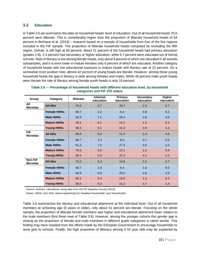
The average household size in the ZOI is 4.7 members. Education levels among the household heads are low. Nearly 70 percent of the household heads are illiterate while only about 25 percent have completed primary education. Rate of literacy and education levels are particularly low among the female heads: 91 % are illiterate, and 7 % have completed primary education.
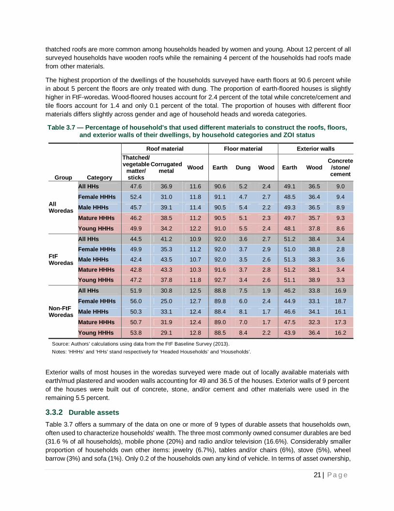
Regarding dwelling characteristics, a large proportion of households in rural areas build their dwellings using locally available materials. Households in the ZOI usually have thatched (45 %) or corrugated iron-sheet (41%) roofs. About 11 percent of all surveyed households have wooden roofs while the remaining 3 percent of the households have roofs made from other materials. Most of the households have earth floors (92 %) while about 4 percent have floors that are only treated with dung. The three most commonly owned consumer durables are bed (35 % of all households in the ZOI), mobile phone (24%) and radio and/or television (19%). Considerably smaller proportion of households owns other items: jewelry (6%), tables and/or chairs (6%), stove (5%), wheel barrow (4%) and sofa (2%). In terms of asset ownership, a typical proxy for wealth in this context, male headed households generally are wealthier than the female headed households.
From the amenities available to households residing in the FtF ZOI, the proportion of households with access to tap water is 36 percent, out of which about one-third use public or shared tap water. On the other hand, about 60 percent of the households have access to reasonable sanitation. Only 6 percent of the households have access to electricity.
Chapter 4: Profile of Economic Activity
This chapter focuses on aspects of production and marketing of crop, livestock and livestock products for households in the ZOI. Land and input use, output quantity, and measures of crop productivity are presented along with production and marketing of livestock and livestock products.
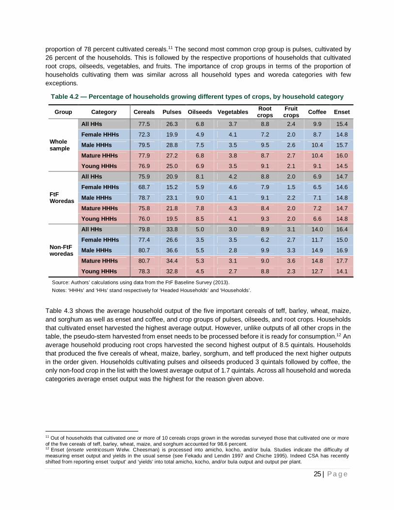
Nearly 90 % of the households cultivated one or more crops during the main agricultural season (meher) of 2012/13. An average household cultivated about a hectare of land which is typically divided into 3 plots. Average output level is calculated for the five important cereals of teff, barley, wheat, maize, and sorghum as well as enset and coffee, and other crop groups for the households in the ZOI. Households that cultivated
vi | P a g e
enset harvested the highest average output (14.5 quintals) followed by root crops (12.2 quintals), while the crop with the least output quantity was teff (3.7 quintals).
The percentage of farmers in the ZOI who adopted chemical fertilizer was around 49 percent. The average fertilizer application rate is around 66 kilograms per hectare (KGs/ha) for all households while it is around 136 KGs/ha for those households who adopted fertilizer. In general, male headed households have a higher adoption rate (52 percent) compared to their female counterparts (41 percent).
The adoption of improved seeds is very low among households in the ZOI. Only 23 percent of households used improved seeds in the main growing season. Households who adopted improved seeds applied about 15 KGs /ha. However, considering all the households in the ZOI who are engaged in crop production, the average application rate was only about 2 KGs/ha. As is the case with fertilizer adoption, fewer female headed households used improved seeds compared to male headed households.
The percentage of households who used irrigation and applied pesticides is only 5 percent and 6 percent, respectively. On the other hand, a relatively higher percentage of households (41 percent) used at least one soil conservation method on their land.
Crop level yield is calculated for major cereals, selected permanent crops and other crop groups. Enset has the highest yield (132 quintals/ha) followed by root crops (95 quintals/ha). Among the major cereals, wheat has the highest yield of 22 quintals/ha followed by maize (20.5 quintals per hectare) while Teff has the lowest yield compared to the other cereals.
Nearly 87 percent of all households in the ZOI own livestock. The average household owns about 4.1 Tropical Livestock Units (TLU). Looking into the milk yield of households, used as a measure of livestock productivity, an average milk producing households produces approximately 0.8 liters of milk per cow per day. The major risks and constraints that households face in livestock production are water shortages, livestock diseases and lack of grazing land.
With regard to marketing of crop output, livestock, and livestock products in the FtF ZOI, slightly higher than a third of the sample households sold part of their produced crop output with notable differences across various crop categories. The percentage of households who sold livestock and livestock products is around 8 percent and 14 percent, respectively.
The average annual revenue generated by households from crop sales is around 4,468 birr. Average annual revenue from livestock sales is the highest for cattle (4, 246 Birr) followed by pack animals (2,842 Birr). In terms of marketing of livestock products, revenue collected from sale of milk is the highest at 12,738 Birr, followed by Butter and yoghurt with a value of 8,185 Birr.
Chapter 5: Poverty
Chapter 5 focuses on measuring the prevalence of poverty and the mean per capita expenditure. To estimates these two figures, detailed expenditure information ranging from weekly to annual expenditure values are collected. Prevalence of poverty - as captured by the percentage of people living with less than $1.25/day in 2005 prices - for the FtF ZOI is estimated to be 34.87% and the mean real annual daily per capita expenditures is computed to be 1.76 Birr- where both are expressed in adult equivalent units. Note that, in comparison with the national estimate, the headcount figures are slightly higher for the reason that the poverty line used in this study is also higher than the national one.
vii | P a g e
Chapter 6: Food Security and Nutrition
This chapter provides an overview of the food security and nutrition situation in the ZOI. The objective indicators display alarming food insecurity in the FtF ZOI. Nearly one-third of the children less than 5 years old are underweight (WHZ < -2), more than half are stunted (HAZ < -2) and about 12 % are suffer from wasting (WAZ < -2). These poor child health outcomes are likely to be linked with poor maternal nutrition and lack of dietary diversity in the households. Indeed, every fourth woman of reproductive age (15-49 year old) is underweight (BMI<18.5). Furthermore, less than 1 % of the children receive minimum acceptable diet. On a slightly more positive note, nearly 70 % of the children less than 6 months of age are exclusively breastfed in the ZOI woredas.
Chapter 7: Women Empowerment in Agriculture Index
The WEAI is a newly developed index by researchers at USAID, IFPRI, and the Oxford Poverty and Human Development Initiative (OPHI) to track the change in women’s empowerment in agriculture levels that occurs as a direct or indirect result of interventions under Feed the Future, the U.S. government’s global hunger and food security initiative. The index is composed of two sub-indices: the five domains of empowerment in agriculture (5DE) and the gender parity in empowerment (GPI). The 5DE is composed of the empowerment of women in five domains, namely, production, resource, income, leadership and time use. A woman is defined as empowered in 5DE if she has adequate achievements in four of the five domains or is empowered in some combination of the weighted indicators that reflect 80 percent of the total adequacy. The second sub-index, the GPI, is a relative inequality measure that reflects the inequality in 5DE profiles between the primary adult male and female in each household. The calculation of GPI excludes households with primary male only. That is, the GPI reflects the relative empowerment gap between the woman’s 5DE score with respect to the man’s. The aggregate index, WEAI, is the weighted average of the 5DE and the GPI in which 5DE sub-index contributes 90 percent of the weight to the WEAI and the rest being GPI.
The WEAI for the sample areas in the FtF ZOI is 0.698 with 0.679 and 0.869 values of 5DE and GPI sub-indices, respectively. The result also reveals that 22 percent of all women are empowered in the five domains and from those who are not empowered, they have adequate achievements in 59 percent of the domains. Moreover, the result indicates that 44 percent of women have gender parity with the primary male in their households. Of the 56 percent of women who do not have gender parity, the empowerment gap between them and the male in their household is 23.5 percent.
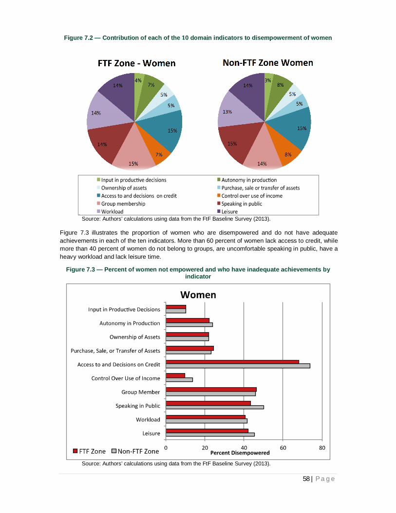
The domains that contribute most to women’s disempowerment in the ZOI are weak leadership and influence in the community (30 %), lack of control over time (28 %), and lack of control over resources (25 %). Within the two largest areas of disempowerment (leadership and time), each sub-indicator contributes nearly equally to disempowerment. Discomfort with speaking in public, lack of participation in groups, heavy workload and lack of leisure time each contribute 13-15 percent to overall disempowerment.
viii | P a g e
Table of Contents Acknowledgements .................................................................................................................................................. ii
Acronyms ................................................................................................................................................................ iii
Executive Summary................................................................................................................................................. iv
Table of Contents .................................................................................................................................................. viii
List of Figures .......................................................................................................................................................... x
List of Tables............................................................................................................................................................ x
4. Profile of economic activity ............................................................................................................................. 24
4.1 Crop Production – Products, inputs, practices, and productivity ................................................................... 24
4.1.1 Cropping patterns and output levels ................................................................................................... 24
4.1.2 Inputs and production practices .......................................................................................................... 26
4.1.3 Land productivity ............................................................................................................................... 32
4.2 Livestock Production – Products and productivity ........................................................................................ 34
4.3 Marketing of crops, livestock and livestock products .................................................................................... 38
4.3.1 Marketing of crop output .................................................................................................................... 38
4.3.2 Marketing of livestock ........................................................................................................................ 41
4.3.3 Marketing of livestock products .......................................................................................................... 41
5.2 Measuring incidence of poverty .................................................................................................................. 44
5.2.1 Determining poverty line .................................................................................................................... 44
5.3 Baseline estimated results for prevalence of poverty and consumption expenditure at FtF ZOI ..................... 45
5.3.1 Indicators for sustainable reduction in global poverty and hunger: Prevalence of Poverty: Percent of people living on less than $1.25/day.................................................................................................................... 45
ix | P a g e
5.3.2 Indicators for First Level Objective 1 – Inclusive Agricultural Sector Growth: Daily per capita expenditures (as a proxy for income) in USG-assisted areas ............................................................................... 46
6. Food Security and Nutrition ............................................................................................................................ 48
6.1 Indicators for sustainable reduction in global poverty and hunger: Prevalence of underweight children under five years of age ..................................................................................................................................................... 48
6.2 Indicators for First Level Objective 2 – Improved nutritional status especially of women and children ............ 49
6.3 Indicators for Intermediate Result 5: Increased Resilience of Vulnerable Communities and Households ....... 50
6.4 Indicators for Intermediate Result 6: Improved Access to Diverse and Quality Foods ................................... 51
6.5 Indicators for Intermediate Result 7: Improved Nutrition-Related Behaviors ................................................. 52
7. Introduction to the women’s empowerment in agriculture index ........................................................................ 53
7.1 Measuring Women’s Empowerment in Agriculture – Approach ................................................................... 53
7.1.1 Purpose of the WEAI ......................................................................................................................... 53
7.1.2 Structure of the WEAI ........................................................................................................................ 53
7.2 Indicators for First Level Objective 1 – Inclusive Agricultural Sector Growth: Women's Empowerment in Agriculture Index .................................................................................................................................................... 56
Appendix A: Appendix to Chapter 2......................................................................................................................... 64
Appendix B: Appendix to Chapter 3......................................................................................................................... 76
Appendix C: Appendix to Chapter 4 ........................................................................................................................ 77
Appendix D: Appendix to Chapter 5 ........................................................................................................................ 86
Appendix E: Appendix to Chapter 6......................................................................................................................... 92
x | P a g e
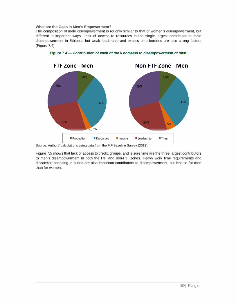
List of Figures Figure 1.1 — Feed the Future in Ethiopia ..................................................................................................................1 Figure 3.2 — Distribution of household size ............................................................................................................. 16 Figure 7.1 — Contribution of each of the 5 domains to disempowerment of women .................................................. 57 Figure 7.2 — Contribution of each of the 10 domain indicators to disempowerment of women .................................. 58 Figure 7.3 — Percent of women not empowered and who have inadequate achievements by indicator ..................... 58 Figure 7.4 — Contribution of each of the 5 domains to disempowerment of men ...................................................... 59 Figure 7.5 — Contribution of each of the 10 domain indicators to disempowerment of men ....................................... 60 Figure 7.6 — Percent of men not empowered and who have inadequate achievements by indicator ......................... 60
List of Tables Table 1.1 — Demographic characteristics of the ZOI .................................................................................................2 Table 1.2 — Selected results for FtF Indicators .........................................................................................................3 Table 2.1 — The Indicators .......................................................................................................................................4 Table 2.2 — Calculation of the double-difference estimate of average program effect .................................................6 Table 2.3 — FtF Sample Woredas – Grouped by FtF Program ................................................................................ 10 Table 2.4 — FtF Sample Households - Planned by Region ...................................................................................... 10 Table 3.1 — Descriptive statistics of household heads’ age, by household categories and ZOI status ....................... 15 Table 3.2 — Proportion of household head marital status, by household categories and FtF ZOI status .................... 16 Table 3.3 — Average household size, by household categories and FtF ZOI status .................................................. 17 Table 3.4 — Percentage of households with average age of members for different age groups, by ZOI and household categories .............................................................................................................................................................. 18 Table 3.5 — Percentage of household heads with different education level, by household categories and FtF ZOI status ..................................................................................................................................................................... 19 Table 3.6 — Percentage of household members by education level, age, and gender .............................................. 20 Table 3.7 — Percentage of household's that used different materials to construct the roofs, floors, and exterior walls of their dwellings, by household categories and ZOI status .......................................................................................... 21 Table 3.8 — Percentage of household head’s asset ownership structure, by household category ............................. 22 Table 3.9 — Percentage of households with access to water, electricity, and sanitation ............................................ 23 Table 4.1 — Number of crops grown, by household type ......................................................................................... 24 Table 4.2 — Percentage of households growing different types of crops, by household category .............................. 25 Table 4.3 — Average crop output (quintals), by household category ........................................................................ 26 Table 4.4 — Total cultivated area and average plot size (ha), by crop type and household categories ....................... 28 Table 4.5 — Average application rate of fertilizer for all farmers and users only (in kg/ha), by household categories .. 29 Table 4.6 —Improved seed application rate (in kg/ha) and percentage of households using improved seeds, pesticides, and irrigation, by household categories and FtF ZOI ............................................................................... 32 Table 4.7 — Average crop yield (quintals/ha), by household category ...................................................................... 33 Table 4.8 — Livestock ownership ............................................................................................................................ 35 Table 4.9 — Average milk yield (liter/cow/day) in milk producing households............................................................ 36 Table 4.10 — Livestock related shocks ................................................................................................................... 37 Table 4.11 — Proportion of Households that sold crops, by FtF ZOI ......................................................................... 38 Table 4.12 — Average household crop sales revenue (Birr), by household categories and FtF ZOI ........................... 38 Table 4.13 — Average household revenue (Birr) per crop, by household categories ................................................. 40 Table 4.14 — Proportion of Households that sold different livestock, by FtF ZOI ....................................................... 41 Table 4.15 — Average and proportion of revenue collected from sale of livestock, by livestock type, household category ................................................................................................................................................................. 41 Table 4.16 — Proportion of Households that sold livestock products, by FtF ZOI ...................................................... 42 Table 4.17 — Average revenue collected from sale of livestock products, by household category ............................. 42
xi | P a g e
Table 5.1 — Poverty headcount (= less than $1.25 in PPP units at 2005 prices), by household type ......................... 46 Table 5.2 — Nominal and real average daily expenditure per capita and per adult equivalent, by household type ...... 47 Table 6.1— Prevalence of underweight in children under 5 years of age .................................................................. 49 Table 6.2— Prevalence of stunted and wasted children under 5 years of age ........................................................... 49 Table 6.3 — Prevalence of underweight women ...................................................................................................... 50 Table 6.4 — Prevalence of households with moderate or severe hunger .................................................................. 50 Table 6.5 — Prevalence of children 6-23 months receiving a minimum acceptable diet, by breastfeeding status ....... 51 Table 6.6 — Women’s dietary diversity ................................................................................................................... 52 Table 6.7 — Prevalence of exclusive breastfeeding of children under six months of age ........................................... 52 Table 7.1 — The 5 domains of empowerment in the WEAI ...................................................................................... 55 Table 7.2 — WEAI results ....................................................................................................................................... 56
1 | P a g e
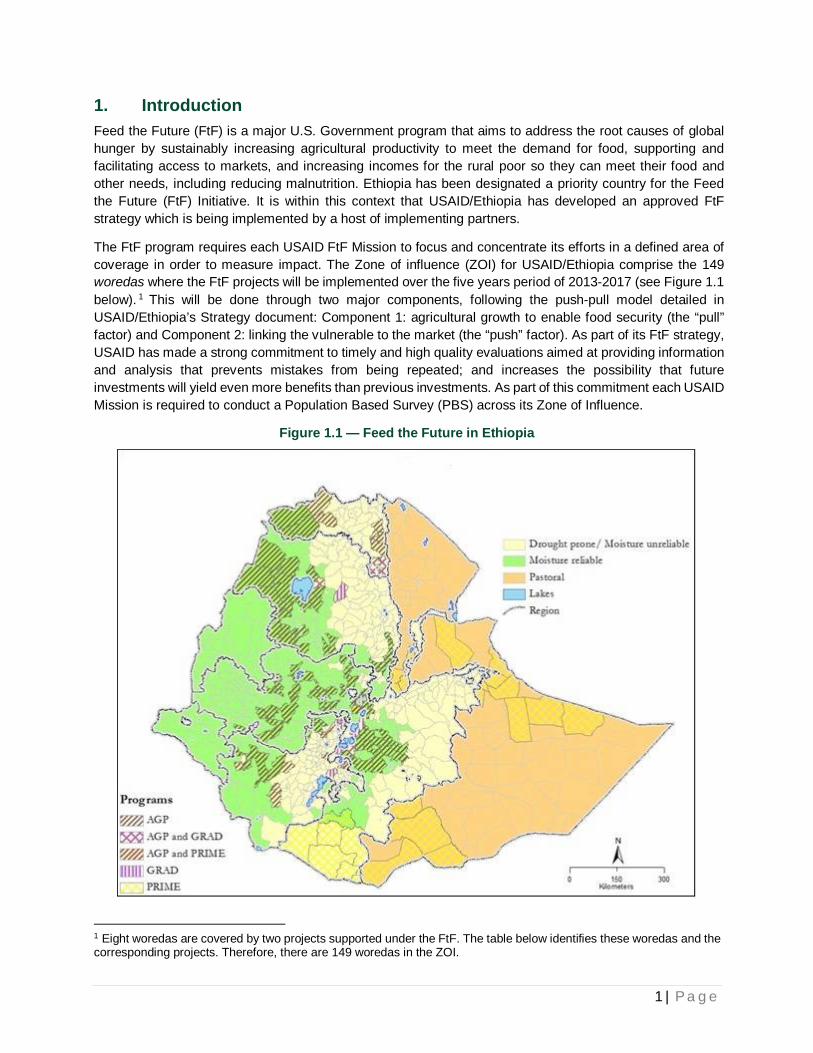
1. Introduction Feed the Future (FtF) is a major U.S. Government program that aims to address the root causes of global hunger by sustainably increasing agricultural productivity to meet the demand for food, supporting and facilitating access to markets, and increasing incomes for the rural poor so they can meet their food and other needs, including reducing malnutrition. Ethiopia has been designated a priority country for the Feed the Future (FtF) Initiative. It is within this context that USAID/Ethiopia has developed an approved FtF strategy which is being implemented by a host of implementing partners.
The FtF program requires each USAID FtF Mission to focus and concentrate its efforts in a defined area of coverage in order to measure impact. The Zone of influence (ZOI) for USAID/Ethiopia comprise the 149 woredas where the FtF projects will be implemented over the five years period of 2013-2017 (see Figure 1.1 below). 1 This will be done through two major components, following the push-pull model detailed in USAID/Ethiopia’s Strategy document: Component 1: agricultural growth to enable food security (the “pull” factor) and Component 2: linking the vulnerable to the market (the “push” factor). As part of its FtF strategy, USAID has made a strong commitment to timely and high quality evaluations aimed at providing information and analysis that prevents mistakes from being repeated; and increases the possibility that future investments will yield even more benefits than previous investments. As part of this commitment each USAID Mission is required to conduct a Population Based Survey (PBS) across its Zone of Influence.
Figure 1.1 — Feed the Future in Ethiopia
1 Eight woredas are covered by two projects supported under the FtF. The table below identifies these woredas and the corresponding projects. Therefore, there are 149 woredas in the ZOI.
2 | P a g e
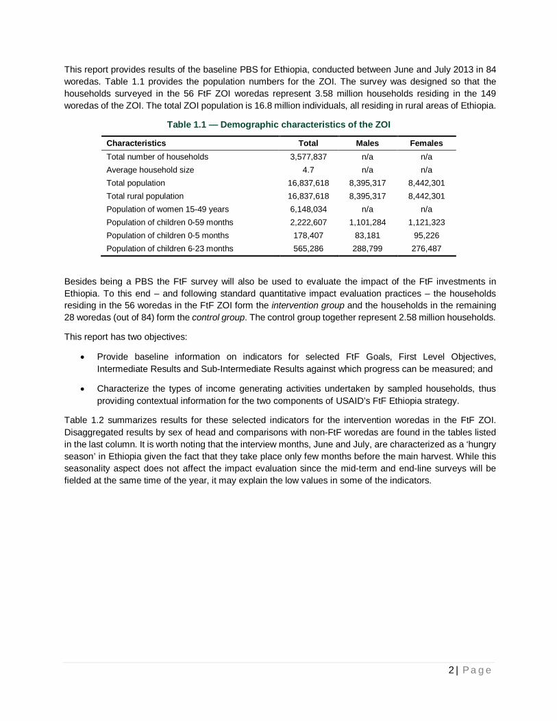
This report provides results of the baseline PBS for Ethiopia, conducted between June and July 2013 in 84 woredas. Table 1.1 provides the population numbers for the ZOI. The survey was designed so that the households surveyed in the 56 FtF ZOI woredas represent 3.58 million households residing in the 149 woredas of the ZOI. The total ZOI population is 16.8 million individuals, all residing in rural areas of Ethiopia.
Table 1.1 — Demographic characteristics of the ZOI
Characteristics Total Males Females Total number of households 3,577,837 n/a n/a Average household size 4.7 n/a n/a Total population 16,837,618 8,395,317 8,442,301 Total rural population 16,837,618 8,395,317 8,442,301 Population of women 15-49 years 6,148,034 n/a n/a Population of children 0-59 months 2,222,607 1,101,284 1,121,323 Population of children 0-5 months 178,407 83,181 95,226 Population of children 6-23 months 565,286 288,799 276,487
Besides being a PBS the FtF survey will also be used to evaluate the impact of the FtF investments in Ethiopia. To this end – and following standard quantitative impact evaluation practices – the households residing in the 56 woredas in the FtF ZOI form the intervention group and the households in the remaining 28 woredas (out of 84) form the control group. The control group together represent 2.58 million households.
This report has two objectives:
Provide baseline information on indicators for selected FtF Goals, First Level Objectives, Intermediate Results and Sub-Intermediate Results against which progress can be measured; and
Characterize the types of income generating activities undertaken by sampled households, thus providing contextual information for the two components of USAID’s FtF Ethiopia strategy.
Table 1.2 summarizes results for these selected indicators for the intervention woredas in the FtF ZOI. Disaggregated results by sex of head and comparisons with non-FtF woredas are found in the tables listed in the last column. It is worth noting that the interview months, June and July, are characterized as a ‘hungry season’ in Ethiopia given the fact that they take place only few months before the main harvest. While this seasonality aspect does not affect the impact evaluation since the mid-term and end-line surveys will be fielded at the same time of the year, it may explain the low values in some of the indicators.
3 | P a g e
Table 1.2 — Selected results for FtF Indicators
Type of Indicator Indicator FtF Woredas Reference (Table)
Goal: Sustainably Reduce Global Poverty and Hunger Poverty headcount 34.8 % 5.1
Prevalence of underweight children under five years of age 32.1 % 6.1
First Level Objective 1: Inclusive Agricultural Sector Growth
Daily per capita expenditures (as a proxy for income) in USG-assisted areas
$1.76 (PPP Dollars) 5.2
Women's Empowerment in Agriculture Index 0.698 7.2
First Level Objective 2: Improved Nutritional Status Especially of Women and Children
Prevalence of stunted children under five years of age 50.6 % 6.2
Prevalence of wasted children under five years of age 12.1 % 6.2
Prevalence of underweight women 26.8 % 6.3
Intermediate Result 5: Increased Resilience of Vulnerable Communities and Households
Prevalence of households with moderate or severe hunger 4.9 % 6.4
Intermediate Result 6: Improved Access to Diverse and Quality Foods
Prevalence of children 6-23 months receiving a minimum acceptable diet
0.56% (Breastfed)
0.00 % (Non-breastfed)
6.5
Women’s Dietary Diversity: Mean number of food groups consumed by women of reproductive age
1.57 % 6.6
Intermediate Result 7: Improved Nutrition-Related Behaviors
Prevalence of exclusive breastfeeding of children under six months of age
67.6 % 6.7
Source: Authors’ calculations using data from the FtF Baseline Survey (2013).
4 | P a g e
2. The Feed the Future Baseline Survey – Methodology and Implementation
2.1 Background
The USAID Mission in Ethiopia contracted the International Food Policy Research Institute (IFPRI) and, through the latter, the Ethiopian Central Statistical Agency (CSA) to carry out the Baseline Survey for Feed the Future Zone of Influence. The baseline survey was conducted in 2013: the first year of the implementation of the FtF-investments in Ethiopia.
Specifically, IFPRI is entrusted with the following tasks:
i. Collect baseline data for the required population-based indicators (PBS) in a sample from 149 Woredas which make up the USAID/Ethiopia FtF ZOI;
ii. Undertake the required midline and endline ZOI surveys and impact analyses over the five years; iii. Establish statistically significant control groups and collect baseline data that will be used to conduct
impact evaluations for selected high-value Mission Programs and Development Objective #1 (see Table 2.1 below for the list of indicators covered).
iv. Use existing survey data to generate interim baseline information on the relevant indicators for the Zone of Influence.
v. Assist USAID to set targets for the indicators below based on the interim and final baseline data;2 vi. Conduct analysis on between five and ten of the FtF Learning Agenda questions at baseline, midline
and endline as appropriate (see Appendix A Tables 2.2-2.4 for the questions).
We begin by explaining how the surveys were designed to provide both the population-based indicators and the baseline for quantitative impact analysis. We describe how this work will contribute to the capacity of Ethiopia’s Central Statistics Agency (CSA) to implement surveys in support of Government of Ethiopia and its development partners.
Table 2.1 — The Indicators
1. Prevalence of Poverty: Percent of people living on less than $1.25/day 2. Per capita expenditures of targeted beneficiaries 3. Prevalence of underweight children under five years of age 4. Prevalence of stunted children under five years of age 5. Prevalence of wasted children under five years of age 6. Prevalence of underweight women 7. Women's Empowerment in Agriculture Index 8. Prevalence of households with moderate or severe hunger 9. Prevalence of children 6-23 months receiving a minimum acceptable diet 10. Women’s Dietary Diversity: Mean number of food groups consumed by women of reproductive age 11. Prevalence of exclusive breastfeeding of children under six months of age 12. Percent change in agriculture GDP *
* IFPRI collects data on percent change in agriculture GDP from national accounts and provide to USAID/Ethiopia along with other indicators.
2 The target setting effort was, as appropriate, guided by Target Setting for Reduction in Prevalence of Poverty, underweight and stunting in Feed the Future Zones of Influence (March 1, 2012), Volume 9, Feed The Future M&E Guidance Series. In this regard, the contributions of IFPRI were restricted to drawing and/or validating of target setting procedures as well as providing and/or scrutinizing the relevant data.
5 | P a g e
2.2 Elements of Survey Design and Evaluation Analysis
Designing and implementing a quantitative survey that both generates population based indicators while also providing the baseline for future impact evaluations is challenging but feasible. We begin by reviewing some general issues associated with quantitative impact evaluations along with a number of complexities arising from the approach to implementation being taken by USAID/Ethiopia. We then discuss sample size calculations and the survey instrument design before explaining the roles played by the CSA and IFPRI in this work.
2.2.1 Aspects of FtF relevant to the design of an impact evaluation strategy Central to USAID’s evaluation of FtF activities is the application of “difference-in-differences” or “double difference” methods to longitudinal data. These methods use baseline data before a programme is implemented and follow-up data after it starts to develop a “before and after” comparison. These data are collected from households or individuals receiving the programme and those that do not (“with the programme”/“without the programme”). To see why both “before/after” and “with/without” data are valuable, consider the following hypothetical situation.
Suppose an evaluation only collected data from beneficiaries, and that in the time between the baseline survey and the follow-up, some adverse event occurred (such as a drought) that makes these households worse off. In such circumstances, beneficiaries may be worse off – the benefits of the programme being more than offset by the damage inflicted by the drought. Alternatively, suppose that another donor funds improvements in roads and this allows households to generate higher incomes. These effects would show up in the difference over time in the intervention group, in addition to the effects attributable to the programme. More generally, restricting the evaluation to only “before/after” comparisons makes it impossible to separate programme impacts from the influence of other events that affect beneficiary households. To ensure that the evaluation of FtF is not adversely affected by such a possibility, it is necessary to know what these indicators would have looked like had the programme not been implemented. Thus, we need a second dimension to our evaluation design which includes data on households “with” and “without” the programme.
To see how the double difference method works, consider Table 2.2. The columns distinguish between households that participate or not in a specific FtF activity (Group I for intervention) and those that do not (Group C for control group). The rows distinguish between before and after the programme (denoted by subscripts 0 and 1). Consider one outcome of interest – say crop yields. Before the programme, we would expect average yields to be similar for the two groups, so that the difference in yields (I0 – C0) would be close to zero. Once the programme has been implemented, however, we expect differences to emerge between the groups, so (I1 – C1) will not be zero. The double-difference estimate is obtained by subtracting the pre-existing differences between the groups, (I0 – C0), from the difference after the programme has been implemented, (I1 – C1). Provided certain conditions are met, this design will take into account pre-existing observable or unobservable differences between the two assigned groups, thus generating average programme effect estimates.
6 | P a g e
Table 2.2 — Calculation of the double-difference estimate of average program effect
Survey round Intervention group (Group I)
Control group (Group C)
Difference across groups
Follow-up I1 C1 I1 – C1
Baseline I0 C0 I0 – C0
Difference across time I1 – I0 C1 – C0 Double-difference (I1 – C1) – (I0 – C0)
Note that the discussion thus far has been somewhat vague on precisely what is meant by the intervention and control groups. To understand how samples of both groups are to be constructed, we need to consider a number of factors specific to the design of FtF interventions in Ethiopia. These are: purposive woreda selection; the demand driven nature of the FtF interventions; household self-selection into FtF activities; the presence of multiple interventions; and spillover effects. We discuss these, and their implications for evaluation, in turn.
Purposive woreda selection: Woredas eligible for the FtF are those with existing location factors that are conducive for agricultural growth (e.g. AGP activities), where investments create a “pull” factor, or those characterized by high levels of chronic food insecurity and/or pastoralist areas, where market components create a “push” factor.
Demand driven FtF interventions and household self-selection: Some of the activities in the FtF projects (such as the AGP) are intended to be demand-driven. Households will choose what activities they will undertake and the extent of their participation. While the woredas where FtF operates are selected, individual farmers themselves choose to be engaged in the program on a voluntary basis. In addition, the individual farmers choose among the options presented. Generally, the role of the village leaders and DAs is only to facilitate the individuals and/or the communities to actively participate in the program and to implement the appropriate activities.
Jointly, these considerations have two implications for survey design and sample size. First, the difference-in-difference methodology requires that at baseline – that is prior to the start of the intervention - intervention and control households are as alike as possible. The USAID/Ethiopia decision to undertake purposive woreda selection means that the two most powerful quantitative impact evaluation methods that would ensure that intervention and control households are alike at baseline – randomized design and regression discontinuity design (which requires a single, strict metric determining woreda eligibility ) – have already been ruled out. Instead, quantitative evaluations will need to use either matching methods or instrumental variables, both of which are more demanding in terms of their data requirements and have higher computational (and therefore analysis time) requirements. 3 In order to use these methods, the survey instruments must – at baseline – collect information on locality, household and individual characteristics that
3 Matching involves the statistical construction of a comparison group of, say households that are sufficiently similar to the treatment group before the program that they serve as a good indication of what the counterfactual outcomes would have been for the treatment group. One popular approach is to match program beneficiaries to a sub-sample of similar non-beneficiaries from the same or neighboring communities using a matching method such as propensity score matching (PSM), nearest neighbor matching or propensity weighted regression. Matching methods choose communities or households as a comparison group based on their similarity in observable variables correlated with the probability of being in the program and with the outcome. All matching methods measure program impact as the difference between average outcomes for treated households and a weighted average of outcomes for non-beneficiary households where the weights are a function of observed variables.
7 | P a g e
affect the decision to participate in an FtF activity in addition to collecting information on FtF indicators. Second, the size of the sample needs to account for the fact that within woredas where FtF is active, not all households will adopt these interventions. A sample of 75 households within an Enumeration Area (EA) is unlikely to be a sample of 75 beneficiaries. If one-third of households adopt the intervention, then the sample of beneficiaries will be 25 households.
Multiple interventions: Participants in FtF may benefit from a single intervention, from multiple interventions and from interventions with differing degrees of intensity. This needs to be taken into account in the evaluation design and implementation.
Spillover effects: The FtF will benefit both program participants and non-participants. For example, even if a household chooses not to actively participate in any FtF activities, it may benefit from FtF activities. For example, consider two households residing in a locality where efforts are being made to increase wheat yields. One household chooses to particpate in these activities; the other does not. However, with wheat yields rising, the participating household (along with other adopters) increases their demand for unskilled labour and this benefits the non-participating household. Suppose we construct a difference-in-difference indicator using the participating household as part of the “intervention group” and the non-participating household as part of the “control group”. Comparing changes in outcome indicators between households that participated in the intervention and those households who did not, will underestimate the impact of the FtF because FtF is indirectly improving outcomes in the control group households. In order to account for these spillover effects, for evaluation purposes, the sample must include woredas which do not receive FtF resources. The presence of potential spillover effects has an important implication for the design of the sample. A survey conducted only in USAID’s Zone of Influence will obtain the required population-based indicators (PBS). Fielding subsequent surveys will generate data that will update these. However, a survey only conducted in USAID’s Zone of Influence cannot provide a robust estimate of FtF’s impact for the reasons described here.
Accordingly, the baseline survey was conducted in woredas in USAID/Ethiopia’s ZOI and also in woredas not within the ZOI. By interviewing households at baseline and at endline both inside and outside of the ZOI and by using a non-experimental impact estimator such as matching, it will be possible to undertake an impact evaluation that determines whether improvements in FtF performance indicators in the ZOI can be attributed to the totality of FtF activities. If these surveys collect information on who participates in the various FtF interventions, it will also be possible to assess both the direct and spillover impacts of FtF. The direct effects are estimated by comparing changes in households that take up FtF interventions with matched households outside the ZOI who, given their characteristics, would have taken up the intervention had it been available. The spillover effects are estimated by comparing changes in households in the ZOI that did not take up FtF interventions with matched households outside the ZOI who, given their characteristics, would not have taken up the intervention even if it had been available. We discuss below whether our sample design can detect other impacts.
2.2.2 Determining sample size The size of the sample depends on a number of considerations. First, is the purpose of the survey to monitor FtF performance indicators or is it to both monitor FtF performance indicators AND provide baseline information for impact evaluation? The survey is designed and conducted to achieve the latter. A note of clarification on indicator tracking is appropriate at this point. The RFA requests disaggregating indicators by household gender and age composition. Specifically, the incidence of poverty, pattern of per capita expenditure, and prevalence of hunger (i.e., Indicators 1, 2, and 8) are to be disaggregated in this way.4 Similarly, Indicator 11 will be disaggregated by gender of children while indicator 9 will be disaggregated by
4 All indicators in this paragraph refer to those listed in Table 1 above
8 | P a g e
gender of children as well as wealth quintiles of households. The sample size required to track indicators and detect impact at these levels of disaggregation would be rather large. Instead, it was agreed that the survey should be designed in such a way that key indicators are, as appropriate, disaggregated by household demographic and wealth characteristics and tracked, though without necessarily aspiring to causal impact evaluation. Obviously, impact at the household level will be assessed in the manner described in the evaluation design section above. Finally, as per the RFA, population counts will be tracked for Indicators 1,3,4,5, and 6. The survey was designed and implemented accordingly.
Second, sample size is affected by the desired level of statistical significance (the sample has to be sufficiently large to minimize the chance of detecting an effect that does not exist) and desired statistical power (the sample has to be sufficiently large to minimize the chance of not detecting an effect that does exist). Following standard practice, these were set at a target level of significance of 5% (two-tailed) and statistical power of 80%.
Sample size also depends on the minimum level of impact the survey is desired to detect in the relevant indicator. For example, should the sample size be large enough to detect that the intervention has reduced poverty by 5 percentage points, by 10 percentage points or by 20 percentage points? These levels of impact, known as minimum detectable effect sizes, are inversely related to sample size. Smaller effect sizes require larger samples; conversely, larger effect sizes require smaller samples. The size of the sample also depends heavily on which FtF indicator is being considered. This is important because required sample sizes are affected by the variability of the indicator. Where the indicator(s) is (are) characterized by high levels of variability, larger sample sizes are needed. It is also affected by what is called the design effect, loosely defined as the extent to which the indicator is correlated across households or individuals within a geographic locality. Higher correlations mean that larger samples are needed.
In addition to all these considerations, the size of the sample depends on precisely what is meant by “FtF impact”. Is FtF impact defined in terms of a particular intervention or is defined in terms of whether the totality of FtF activities in the ZOI leads to changes in performance indicators that can be attributed to FtF?
Finally, we need to take into account the fact that over time some households will move, all members will disperse to other households or the household will chose not to continue to be interviewed. Based on our experiences with other longitudinal household surveys in rural Ethiopia, we assume that ten percent of the sample will attrite between baseline and endline.
A central high-level objective of the FtF initiative is poverty reduction. In light the broad outline of FtF targets in Ethiopia, it is reasonable to opt for a sample size large enough to detect a 10 percentage point reduction in the incidence of poverty linked to FtF.5 The sample size was thus chosen to be large enough to detect this level of impact. This minimum detectable size effect is equivalent to a 22 percent (0.22) standard deviation of poverty reduction in FtF areas over and above that achieved in comparable but non-FtF areas.6 The sample is divided into two-third treated (FtF ZOI) and one-third control (non-FtF ZOI) woredas. The sample is clustered at the woreda level. The aim is ensuring that by the endline, there are on average 75 households interviewed per woreda, with these allocated across three Enumeration Area (EAs) each containing 25 households. We calculated the design effect as equaling 8.4.
5 The incidence of poverty measured by the head count ratio calculated using the PPP poverty line of 1.25 dollars per day. Note also that in the FtF’s guidance notes on target setting, it is stated that in Ethiopia, FtF should reduce the prevalence of poverty from 39.0 to 27.3 percent over a five year period. 6 Calculations using Ethiopian Household Income and Expenditure surveys show that the standard deviation of poverty incidence is around 0.45 and so a 22 percent reduction in this is equivalent to a ten percentage point reduction in poverty.
9 | P a g e
In summary:
Minimum detectable effect size - 10 percentage point reduction in the incidence of poverty linked to FtF;
Statistical significance – 5 percent
Statistical power – 80 percent
Design effect - 8.4
Enumeration Areas (EA) – 3 per woreda
Attrition – 10 percent with 75 households per woreda in the endline survey
Given these features and assumptions, 56 woredas in the FtF ZOI and 28 woredas outside the ZOI are required. In the baseline, 84 households were selected for interview per woreda or 28 households per EA; given an assumed rate of attrition of 10 percent, this will mean that on average, at endline, there will be 75 households interviewed in each woreda. Therefore, the baseline survey was planned to collect information from 4,704 households in the ZOI (56 woredas x 3 EAs per woreda x 28 households per EA) and 2,352 households outside the ZOI (28 woredas x 3 EAs per woreda x 28 households per EA) giving a total baseline sample of 7,056 households residing in 252 EAs (with each EA located in a corresponding kebele).
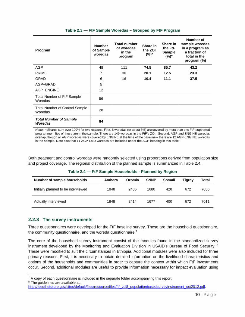
Heterogeneity A number of sources of heterogeneity were considered in the design of the sample. First, the FtF’s ZOI spans woredas with diverse agro-ecological potential. In line with this heterogeneity, the non-ZOI woredas were drawn from a set purposively defined to have characteristics similar to woredas found in the ZOI. Moreover, the woreda composition of the sample was made to reflect the distribution of FtF-supported projects by using the percentage of FtF’s ZOI (or woredas) each major FtF project covers as a basis of its share in the sample (see Table 2.3 below).
Second, households within a locality differ in terms of dimensions that may be relevant to the performance of FtF-related investments. Two such dimensions can be specifically important – the gender and age of household heads. Accordingly, the household composition of the sample in each EA will be determined by the distribution of household types in the community as defined by the gender and age of household heads (see the discussion in Appendix A1 for further detail). This is particularly relevant for the Women Empowerment in Agriculture Index (WEAI).
10 | P a g e
Table 2.3 — FtF Sample Woredas – Grouped by FtF Program
Notes: * Shares sum over 100% for two reasons. First, 8 woredas (or about 5%) are covered by more than one FtF-supported programme – five of these are in the sample. There are 149 woredas in the FtF’s ZOI. Second, AGP and ENGINE woredas overlap, though all AGP woredas were covered by ENGINE at the time of the baseline – there are 12 AGP-ENGINE woredas in the sample. Note also that 11 AGP-LMD woredas are included under the AGP heading in this table.
Both treatment and control woredas were randomly selected using proportions derived from population size and project coverage. The regional distribution of the planned sample is summarized in Table 2.4.
Table 2.4 — FtF Sample Households - Planned by Region
Number of sample households Amhara Oromia SNNP Somali Tigray Total
Initially planned to be interviewed 1848 2436 1680 420 672 7056
Actually interviewed 1848 2414 1677 400 672 7011
2.2.3 The survey instruments Three questionnaires were developed for the FtF baseline survey. These are the household questionnaire, the community questionnaire, and the woreda questionnaire.7
The core of the household survey instrument consist of the modules found in the standardized survey instrument developed by the Monitoring and Evaluation Division in USAID’s Bureau of Food Security. 8 These were modified to suit the circumstances in Ethiopia. Additional modules were also included for three primary reasons. First, it is necessary to obtain detailed information on the livelihood characteristics and options of the households and communities in order to capture the context within which FtF investments occur. Second, additional modules are useful to provide information necessary for impact evaluation using 7 A copy of each questionnaire is included in the separate folder accompanying this report. 8 The guidelines are available at: http://feedthefuture.gov/sites/default/files/resource/files/ftf_vol8_populationbasedsurveyinstrument_oct2012.pdf.
matching methods. Finally, such data are also required towards answering some of the questions in FtF’s Learning Agenda. Each household questionnaire’s modules comprise (the additional modules are marked with asterisk):
Module A: Household Identification
Module B: Informed Consent
Module C: Household Roster and Demographics
Module D: Dwelling Characteristics
Module E: Household Consumption expenditure
Module F: Household Hunger Scale
Module G: Role in Household Decision-making around Production and Income Generation
Module H: Women’s Dietary Diversity and Anthropometry
Module I: Child Anthropometry and Infant and Young Child Feeding
Module O: Employment, Agricultural Productivity and Input Use *
Module P: Crop Utilization *
Module Q: Agricultural Extension, Technology and Information Networks *
Module R: Livestock Ownership and Income from Livestock and Livestock Products *
Module S: Shocks *
Module T-A: Non-Farm Income and Business Activities – Own Business Activities *
Module T-B: Off-Farm Employment *
Module T-C: Credit *
Module U: Trust, Control and Agency *
Module V: Resilience *
Module X: Household Assets (Non-Land) *
The community questionnaire provides information on community- or kebele-level resources that will affect take-up of FtF interventions. The questionnaire was admistered to at least five people who are knowledgeable about the community (e.g., community leaders, PA chairmen, elders, priests, teachers). To ensure representatives at least one woman and a representative of youth had to be included. Modules in the community questionnaire include:
Site identification
Location and access
Water and electricity
Household assets
12 | P a g e
Services (general)
Education and health services
Production, marketing and extension
Migration
Local wages
Food prices in the last year
Government of Ethiopia and/or FtF programs/projects operating in the locality or kebele (eg the PSNP, AGP)
Current food prices
The woreda questionnaire is aimed at understanding the context and process of the implementation of FtF projects (AGP, GRAD, ENGINE, PRIME and PSNP) at the woreda level. For this reason, it targets woreda officials who have involvement with, and knowledge of, how these projects operate in each woreda. Specifically, Heads of the Woreda Office of Agriculture (WOA) and the Woreda Office of Finance and Economic Development (WOFED) in each woreda were interviewed.
The CSA taskforce and the IFPRI team worked jointly on the preparation of survey instruments based on the generic FtF household questionnaire. These preparations included the translations of all survey instruments from English to Amharic. Before the actual field work, IFPRI research staff, CSA staff and 30 IFPRI-hired supervisors commented on the household questionnaire. The first paper-questionnaire-based training of trainers helped to refine the survey instrument further.
In parallel, the CAPI version was developed as CSPro application or program. The program was put through a series of rigorous tests and modified as necessary. This process continued until the end of the enumerators’ training process.
The expected timespan of the survey preparation phase was March 6 - May 12, 2013. The phase was actually completed on May 17, 2013. Note, however, that revisions of the household questionnaire, particularly the CAPI version, continued beyond this date until the end of the enumerators’ training process.
2.2.4 Survey implementation Training and data collection constitute the two key tasks of this phase – training and data collection.
Training
Training CSA supervisors and enumerators took place during May 20 – June 8, 2013 in five CSA branch offices. As stipulated, CSA staff from its head office conducted the training. They were supported by the IFPRI team and the IFPRI-hired supervisors. The IFPRI supervisors also helped the trainers during the discussion.
The training was organized in two parts. The first part focused on the substantive aspects of the questionnaires module by module and was based on the paper versions of the questionnaires. Part two of the training introduced the CAPI version of the household questionnaire to supervisors and enumerators. It also served as a means of identifying programming problems. Data collection and transfer protocols have been part of the training program. This was particularly true of the household questionnaire which was implemented in digital form. A field pilot at the end helped reinforce what was learnt during training as well as finding any remaining bugs in the program. Both parts were successfully implemented during May 20 – June 8, 2013 as planned.
13 | P a g e
Data collection
Data were collected using the three questionnaires described earlier – household, community (with price modules), and woreda questionnaires. As noted above, CSA had the responsibilty for survey implementation with IFPRI providing technical support. Twenty-seven IFPRI-hired supervisors participated in the process. The IFPRI team also travelled to sample sites to assess implementation and to help solve unanticipated problems on the field. These two supportive roles of IFPRI proved crucial, particularly for data saving and transfer.
A major task embedded with data collection was data transfer. The digital household data collected using CAPI questionnaire had to be regularly transferred to the CSA during the data collection period. Three objectives were to be achieved by doing so: to detect and correct collection errors as quickly as possible; to reduce the likelihood of data loss; and to maintain the integrity of the collected data. A purposely designed transfer protocol was adopted.
Data transfer from the field was planned to start as soon as data collection began. It did so only in a small number of cases. A lot of time and effort were needed to ensure all CSA branches transfer data the same way. Indeed, this effort continued for a number of weeks after the end of data collection.
The planned length of the data collection was 28 days during June 14 – July 12, 2013.9 This was achieved in many areas. However, additional days were required in some woredas due to longer travel time and the use of paper questionnaire. More significantly, data transfer took much longer than anticipated. The lack of requisite technical knowledge and experience led to a long iterative process of obtaining the collected data from CSA branch offices. The process continued even after the data were at the CSA headquarters because of the need to resolve problems discovered during the compilation of the database. As consequence, CSA was able to officially deliver the raw household data to IFPRI on August 24, 2013. The filled community questionnaires were received by IFPRI in batches in the weeks that followed.
Outcomes
In the end, data from 7011 households, 250 kebeles and 84 woredas were collected.
As expected, the FtF baseline survey provided a good opportunity to improve CSA’s capacity to conduct large CAPI-based surveys. This capacity grew substantially in three major ways – equipment, skills, and organization:
CSA obtained a total of 561 netbooks which will be available for future surveys;10
84 supervisors and 38 statisticians (all permanent employees of the Agency) and 280 enumerators received CAPI training and acquired field experience in using those skills.
CSA was able to identify the challenges CAPI-based surveys pose to its IT system and is working towards meeting the demands of secure digital data transfer during actual data collections.
9 A survey period during June-July reflects the window available in the busy CSA schedule and the longer front-end preparation required by the CAPI approach. Being a busy period in many agricultural communities, the timing is not without problems. Accordingly, the CSA designed and adopted an interview protocol that required enumerators to chart an interview schedule in consultation with sample households at the beginning and ensure that a single interview session do not exceed 2 hours. Moreover, the CSA has acquired a lot of experience (partly through joint work with IFPRI such the PSNP and AGP surveys) of conducting effective surveys during these months. 10 These include the 305 netbooks added for Agricultural Growth Program (AGP) midline survey and financed out of the FtF baseline budget.
14 | P a g e
3. Characteristics of Households This chapter describes the households in the FtF baseline survey in terms of their demographic characteristics, their durable asset ownership, and amenities available to them. The chapter has five sections. The first sections discuss the respective four dimensions while the final section summarizes the chapter. For this purpose we use household level data collected in the FtF baseline survey.
3.1 Household demography
Table 3.1 summarizes the data on household heads' age across household and woreda categories while Figure 3.1 summarizes the data across detailed age categories. At the time of the survey, the average age of a household head was about 43 years with half of the heads being 39 years old or younger (Table 3.1). Households with young heads (less than 35 years of age) accounted for 38 percent of the total with heads younger than 20 years accounting for 0.4 percent and had an average age of 18 years (Figure 3.1). About 5 percent of the household heads were 70-79 years old and had an average age of 72 years while heads 80 or older accounted for 2 percent and were on average 85 years old.
Figure 3.1 — Age structure of household heads
Source: Authors’ calculations using data from the FtF Baseline Survey (2013). Note: the numbers in the parentheses refer to the mean age for the given age category.
Out of the households in the woredas surveyed 28 percent had female heads. Consistent with patterns in household heads’ ages observed in other works using comparable data, female heads are on average older than their male counterparts (see Berhane et al. 2013). Out of the 28 percent female heads 26 percent were mature (35 years or older) or only 6 percent of the heads were both female and young (15-34 years of age). The proportion of mature-male and young-male heads is 40 and 32 percent, respectively.
Under 20 (18),0.4%
Ages 20-29 (26), 17%
Ages 30-39 (34), 33%
Ages 40-49 (43), 17%
Ages 50-59 (53), 15%
Ages 60-69 (63), 11%
Ages 70 and above (76), 7%
15 | P a g e
Table 3.1 — Descriptive statistics of household heads’ age, by household categories and ZOI status
Group Category Proportion of HHs
Statistics on household head’s age
Mean SD Median
All Woredas
All HHs 100 42.7 15 39
Female HHHs 27.9 47 14.8 48
Male HHHs 72.1 41 14.7 36
Mature HHHs 61.8 51.2 12.8 50
Young HHHs 38.1 29 3.8 30
FtF Woredas
All HHs 58.1 42.4 14.8 38
Female HHHs 28.1 46.7 14.6 47
Male HHHs 71.9 40.7 14.6 36
Mature HHHs 61.3 50.9 12.7 50
Young HHHs 38.7 28.9 3.9 30
Non-FtF Woredas
All HHs 41.9 43.2 15.2 40
Female HHHs 27.7 47.5 15.1 50
Male HHHs 72.3 41.5 14.9 37
Mature HHHs 62.6 51.6 13 50
Young HHHs 37.4 29.1 3.7 30
Source: Authors’ calculations using data from the FtF Baseline Survey (2013). Notes: ‘HHHs’ and ‘HHs’ stand respectively for ‘Headed Households’ and ‘Households’. ‘SD’ stands for ‘Standard Deviation’. ‘Mature HHH’ refers to household headed by 35 years of age or older individuals and ‘Young HHH’ to households headed by 15-34 year old individuals.
In the full sample, 74 percent of the heads are married to single or multiple spouses (Table 3.2). About 7 percent of the heads are either divorced or separated while 16 percent are widowed. The difference in marital status of female and male heads is considerable. While only 23.4 percent of female household heads were married, the corresponding proportion is 94 percent in male heads. Moreover, about 23 percent of female heads are divorced/separated and 52 percent were widowed. This confirms the common observation that women become household heads in rural Ethiopia usually after being separated with their spouse for one or another reason. The proportion of married younger heads is higher relative to mature heads, while the proportion divorced, separated or widowed is considerably higher among the latter.
16 | P a g e
Table 3.2 — Proportion of household head marital status, by household categories and FtF ZOI status
Group Category Married, single
spouse Single Divorced Widowed Separated
Married, more than
one spouse
All Woredas
All HHs 68.1 1.8 5.8 15.9 2.3 6.2
Female HHHs 17.4 1.8 16.2 51.7 6.8 6.1
Male HHHs 87.8 1.7 1.7 2.0 0.5 6.2
Mature HHHs 60.7 0.3 5.7 23.4 2.5 7.5
Young HHHs 80.2 4.2 6.0 3.8 1.9 3.9
FtF Woredas
All HHs 68.1 1.8 5.8 15.9 2.3 6.2
Female HHHs 18.8 1.8 15.6 50.4 6.6 6.9
Male HHHs 86.9 2.0 1.6 2.0 0.8 6.7
Mature HHHs 59.9 0.3 5.8 23.0 2.6 8.4
Young HHHs 80.1 4.5 5.2 4.0 2.0 4.2
Non-FtF Woredas
All HHs 68.7 1.5 6.1 16.3 2.1 5.3
Female HHHs 15.4 1.9 17.2 53.4 7.2 4.9
Male HHHs 89.1 1.4 1.8 2.1 0.2 5.4
Mature HHHs 61.7 0.2 5.5 23.9 2.4 6.3
Young HHHs 80.4 3.8 7.0 3.5 1.7 3.6
Source: Authors’ calculations using data from the FtF Baseline Survey (2013). Notes: ‘HHHs’ and ‘HHs’ stand respectively for ‘Headed Households’ and ‘Households’.
Table 3.3 summarizes the data on household size across household gender, age, and woreda categories while Figure 3.2 provides a slightly detailed summary. An average household in the sample has 4.6 members (Table 3.3). The proportion of single-member households is 4 percent. The proportion of households increases with number of members until 4 members and then declines continuously.
Figure 3.2 — Distribution of household size
Source: Authors’ calculations using data from the FtF Baseline Survey (2013).
1 member4%
2 members13%3 members
16%
4 members18%
5 members17%
6 members14%
7 members9%
8 members5%
9 or more members
4%
17 | P a g e
Relative to other categories, male headed households have the highest number of members followed by those with mature heads, both of which are dominated by households with 5-6 members. Next in household size are young headed households, among which a higher proportion have 3-4 members while the average size of female headed households is the smallest because a relatively large proportion of female headed dominated by households with relatively few members.
Table 3.3 — Average household size, by household categories and FtF ZOI status
Group Category 1-2 members
3-4 members
5-6 members
7-8 members
9-10 members
11 or more Average
All Woredas
All HHs 17.0 33.7 30.8 14.2 3.6 0.7 4.6
Female HHHs 34.7 38.0 20.9 5.3 1.0 0.1 3.5
Male HHHs 10.1 32.1 34.6 17.7 4.6 1.0 5.1
Mature HHHs 16.9 28.2 31.1 17.7 5.0 1.1 4.9
Young HHHs 17.0 42.7 30.4 8.6 1.2 0.1 4.2
FtF Woredas
All HHs 16.3 33.1 30.4 15.1 4.1 0.9 4.7
Female HHHs 32.3 38.4 21.4 6.2 1.5 0.2 3.6
Male HHHs 10.1 31.1 33.9 18.6 5.2 1.1 5.1
Mature HHHs 15.8 27.3 30.9 18.9 5.8 1.3 5.0
Young HHHs 17.1 42.4 29.6 9.1 1.6 0.2 4.2
Non-FtF Woredas
All HHs 17.8 34.5 31.3 13.0 2.8 0.6 4.5
Female HHHs 38.0 37.4 20.3 4.0 0.4 0.0 3.4
Male HHHs 10.1 33.5 35.6 16.4 3.7 0.8 5.0
Mature HHHs 18.4 29.3 31.3 16.0 4.0 0.9 4.7
Young HHHs 16.7 43.3 31.5 7.9 0.6 0.0 4.2
Source: Authors’ calculations using data from the FtF Baseline Survey (2013). Notes: ‘HHHs’ and ‘HHs’ stand respectively for ‘Headed Households’ and ‘Households’.
We summarize the data on household members’ age in Table 3.4 and Figure 3.3. The average age of a household member is 21 years (Table 3.4). Out of residents of the woredas surveyed, 13 percent were under 5 years and their age averaged 2.3 years while the average age of the remaining was 24 years. Out of those with ages of 5 and older, a slightly higher proportion of 44 percent were under 20 years (Figure 3.3). Household members 20 or older accounted for 43 percent of the total and the proportion of members in each 10-year category continuously declines with age.
18 | P a g e
Figure 3.3 — Age structure of household members
Source: Authors’ calculations using data from the FtF Baseline Survey (2013).
The 5-15 year old population constituted the largest block implying more than half of the population in the woredas surveyed was 15 years or younger. The proportion in the next three age categories of 16-24, 25-34, and 35-59 are close to each other ranging between 14.7 and 15.5 percent (Table 3.4).
Table 3.4 — Percentage of households with average age of members for different age groups, by ZOI and household categories
Group Category Under 5 Ages 5-15
Ages 16-24
Ages 25-34
Ages 35-59
Ages 60 or more
Average age (all
members)
Average age (5 years
or older)
All Woredas
All HHs 13.1 36.4 14.7 15.5 15.3 4.9 21.3 24.1
Female HHHs 8.1 39.5 17.6 9.8 17.0 7.9 23.4 25.3
Male HHHs 14.4 35.5 13.9 17.1 14.9 4.1 20.7 23.8
Mature HHHs 8.7 38.8 15.4 6.9 23.0 7.2 24.0 26.1
Young HHHs 21.5 31.9 13.3 31.9 0.9 0.6 16.1 19.9
FtF Woredas
All HHs 13.6 37.1 14.3 15.4 15.1 4.5 20.8 23.7
Female HHHs 9.0 40.2 16.6 9.8 16.7 7.6 22.9 25.0
Male HHHs 14.9 36.2 13.6 16.9 14.6 3.7 20.2 23.4
Mature HHHs 9.4 39.8 14.6 7.0 22.6 6.7 23.4 25.6
Young HHHs 21.6 32.0 13.7 31.2 1.0 0.4 15.9 19.7
Non-FtF Woredas
All HHs 12.3 35.4 15.3 15.8 15.7 5.5 21.9 24.7
Female HHHs 6.9 38.5 19.0 9.9 17.4 8.3 24.2 25.8
Male HHHs 13.7 34.6 14.3 17.3 15.3 4.8 21.4 24.4
Mature HHHs 7.6 37.4 16.7 6.8 23.7 7.9 46.2 46.2
Young HHHs 21.2 31.7 12.7 32.9 0.7 0.9 24.9 26.7
Source: Authors’ calculations using data from the FtF Baseline Survey (2013). Notes: ‘HHHs’ and ‘HHs’ stand respectively for ‘Headed Households’ and ‘Households’.
Under 513%
Ages 5-918%
Ages 10-1926%
Ages 20-2915%
Ages 30-3912%
Ages 40-496%
Ages 50-595%
Ages 60 and above
5%
19 | P a g e
3.2 Education
In Table 3.5 we summarize the data on household heads' level of education. Out of all household heads 70.6 percent were illiterate. This is considerably higher than the proportion of illiterate household heads of 54 percent in Berhane et al. (2013) – research based on a sample of households from four of the five regions included in the FtF sample. The proportion of illiterate household heads computed by excluding the fifth region, Somali, is still high at 65 percent. About 21 percent of the household heads had primary education (grades 1-8), 2.3 percent had secondary or higher education, while 5.7 percent were educated out of formal schools. Rate of literacy is low among female heads, only about 9 percent of which are educated in all woreda subsamples, and it is even lower in mature females only 6 percent of which are educated. Another category of household heads with low educational exposure is mature heads with literacy rate of 22 percent. On a somewhat more positive note, almost 42 percent of young heads are literate. However, among these young household heads the gap in literacy is wide among females and males. While 46 percent male-youth heads were literate the rate of literacy among female-youth heads is only 19 percent.
Table 3.5 — Percentage of household heads with different education level, by household categories and FtF ZOI status
Group Category Illiterate Informal education
Primary education
Secondary education
Higher education
All Woredas All HHs 70.6 5.7 20.7 2.3 0.7
Female HHHs 90.7 2.2 6.2 0.8 0.2
Male HHHs 62.8 7.1 26.4 2.8 0.9
Mature HHHs 78.1 6.1 14.2 1.2 0.3
Young HHHs 58.4 5.1 31.3 3.9 1.3 FtF Woredas All HHs 69.6 6.0 21.4 2.3 0.8
Female HHHs 90.7 2.3 6.0 0.7 0.3
Male HHHs 61.3 7.4 27.4 3.0 1.0
Mature HHHs 76.6 6.6 15.1 1.2 0.4
Young HHHs 58.4 5.0 31.3 4.1 1.3 Non-FtF Woredas All HHs 72.0 5.3 19.8 2.2 0.7
Female HHHs 90.7 1.9 6.4 1.0 0.0
Male HHHs 64.9 6.6 25.0 2.6 0.9
Mature HHHs 80.1 5.4 13.0 1.2 0.2
Young HHHs 58.5 5.2 31.2 3.7 1.4
Source: Authors’ calculations using data from the FtF Baseline Survey (2013). Notes: ‘HHHs’ and ‘HHs’ stand respectively for ‘Headed Households’ and ‘Households’.
Table 3.6 summarizes the literacy and educational attainment at the individual level. Out of all household members at schooling age (5 years or older), only about 41 percent are literate. Focusing on the whole sample, the proportion of illiterate female members was higher and educational attainment lower relative to the male members (first three rows of Table 3.6). However, among the younger cohorts this gender gap is closing as the proportion of female and male members in different grade categories is rather similar. This finding may have resulted from the efforts made by the Ethiopian Government to encourage households to send girls to schools. Finally, the high proportion of illiteracy among 5-10 year olds may be explained by
20 | P a g e
young age or delay in sending children to school. However, the proportion of 10-14 year olds illiterate in this sample is high, almost twice the proportion in Berhane et al. (2013).
Table 3.6 — Percentage of household members by education level, age, and gender
Category Illiterate Informal education
Primary education
Secondary education
Higher education
All Woredas: 60.6 3.4 32.3 3.2 0.5
Male 53.8 4.4 37.1 4.0 0.7
Female 67.4 2.4 27.5 2.3 0.2
5-9 years:
Male 79.3 4.2 16.5 0.0 0.0
Female 76.2 5.2 18.6 0.0 0.0
10-14 years:
Male 34.5 2.9 62.4 0.2 0.0
Female 33.3 2.8 63.4 0.5 0.0
15-24 years:
Male 28.8 1.6 57.4 11.1 1.2
Female 42.0 0.6 47.5 9.2 0.7
25-64 years:
Male 59.8 6.4 28.0 4.5 1.3
Female 87.5 1.9 9.1 1.2 0.2
65 and above:
Male 84.8 8.5 5.9 0.7 0.0
Female 98.7 0.9 0.4 0.0 0.0
Source: Authors’ calculations using data from the FtF Baseline Survey (2013).
Table 3.1 of Appendix B provides a slightly more detailed account of participation in education among the 5-18 year old household members. Among the latter group of household members the rate of literacy is higher and increases consistently up to the 15-16 year age category. The proportion of girls 18 years or younger educated is slightly higher relative to male members.
3.3 Asset ownership
In this section we describe the households in terms of the materials out of which their houses are made of and their durable assets ownership, both of which are often used to characterize households’ wealth in rural areas. Table 3.7 provides a summary of households' dwellings while Table 3.8 does the same for households’ durable asset ownership.
3.3.1 Housing characteristics A large proportion of households in rural areas build their dwellings using locally available materials. Wealthy households typically build their houses from materials often used in urban areas such as corrugated iron and tile roofs, brick and stone/concrete walls, and cement or tile floors. Corrugated iron-sheet roof, an indicator of wealth, is somewhat more common in the FtF-woredas (41%) than in the non-FtF woredas (31%). Most households (48%) in the surveyed woredas have thatched roofs usually made from cereal straws. These
21 | P a g e
thatched roofs are more common among households headed by women and young. About 12 percent of all surveyed households have wooden roofs while the remaining 4 percent of the households had roofs made from other materials.
The highest proportion of the dwellings of the households surveyed have earth floors at 90.6 percent while in about 5 percent the floors are only treated with dung. The proportion of earth-floored houses is slightly higher in FtF-woredas. Wood-floored houses account for 2.4 percent of the total while concrete/cement and tile floors account for 1.4 and only 0.1 percent of the total. The proportion of houses with different floor materials differs slightly across gender and age of household heads and woreda categories.
Table 3.7 — Percentage of household's that used different materials to construct the roofs, floors, and exterior walls of their dwellings, by household categories and ZOI status
Group Category
Roof material Floor material Exterior walls Thatched/ vegetable
Source: Authors’ calculations using data from the FtF Baseline Survey (2013). Notes: ‘HHHs’ and ‘HHs’ stand respectively for ‘Headed Households’ and ‘Households’.
Exterior walls of most houses in the woredas surveyed were made out of locally available materials with earth/mud plastered and wooden walls accounting for 49 and 36.5 of the houses. Exterior walls of 9 percent of the houses were built out of concrete, stone, and/or cement and other materials were used in the remaining 5.5 percent.
3.3.2 Durable assets Table 3.7 offers a summary of the data on one or more of 9 types of durable assets that households own, often used to characterize households' wealth. The three most commonly owned consumer durables are bed (31.6 % of all households), mobile phone (20%) and radio and/or television (16.6%). Considerably smaller proportion of households own other items: jewelry (6.7%), tables and/or chairs (6%), stove (5%), wheel barrow (3%) and sofa (1%). Only 0.2 of the households own any kind of vehicle. In terms of asset ownership,
22 | P a g e
male headed households are generally wealthier than the female headed households. Some differences exist also between the FtF and non-FtF woredas.
Table 3.8 — Percentage of household head’s asset ownership structure, by household category
Source: Authors’ calculations using data from the FtF Baseline Survey (2013). Notes: ‘HHHs’ and ‘HHs’ stand respectively for ‘Headed Households’ and ‘Households’.
3.4 Amenities
This section discusses the amenities available to household members in the woredas surveyed. Table 3.9 provides a summary of the proportion of households with an access to different services.
The proportion of households with access to tap water is 32.4 percent, out of which 31.2 percent use public or shared tap water. About 24 percent of the households have an access to protected borehole, well, and spring water sources. Furthermore, the proportion of households with access to potables water sources in this sample is slightly higher than the nationwide proportion of rural households with access to potable water within 1.5 kilometers of their residences, which is 55 percent (MoFED 2013).
About 57 percent of the households have access to reasonable sanitation. The proportion of male and mature headed households with access to sanitation was higher in all woreda subsamples relative to female and young headed households, respectively. A slightly higher proportion of FtF woreda households have access to sanitation. Finally, only 4 percent of the households in all surveyed woredas have access to electricity. The access to electricity seems to be considerably better in the FtF woredas than in the non-FtF woredas.
23 | P a g e
Table 3.9 — Percentage of households with access to water, electricity, and sanitation
Group Category Access to tap water
Access to protected well/borehole/spring
Access to sanitation
Access to Electricity
All Woredas
All HHs 32.4 24.3 57.3 4.0
Female HHHs 31.5 25.0 52.2 4.1
Male HHHs 32.7 24.0 59.3 3.7
Mature HHHs 31.8 24.1 57.7 3.8
Young HHHs 33.3 24.6 56.6 4.3
FtF Woredas
All HHs 35.5 19.8 60.0 5.9
Female HHHs 35.8 19.6 55.4 5.6
Male HHHs 35.4 19.8 61.8 6.0
Mature HHHs 35.4 19.4 60.7 5.6
Young HHHs 35.7 20.4 59.0 6.4
Non-FtF Woredas
All HHs 28.0 30.5 53.5 1.4
Female HHHs 25.5 32.7 47.6 0.9
Male HHHs 28.9 29.6 55.8 1.6
Mature HHHs 26.9 30.4 53.7 1.3
Young HHHs 29.9 30.6 53.2 1.5
Source: Authors’ calculations using data from the FtF Baseline Survey (2013). Notes: ‘HHHs’ and ‘HHs’ stand respectively for ‘Headed Households’ and ‘Households’.
24 | P a g e
4. Profile of economic activity Agriculture lies at the heart of rural life in Ethiopia. Nationally, over 80 percent of Ethiopians reside in rural areas and depend on agriculture as their main source of income. Moreover, agriculture contributed 44 percent of the GDP in 2011/12 (National bank of Ethiopia 2013). The principal goal of Feed the Future initiative is agriculture led growth with the aim of enabling food security in Ethiopia. This chapter aims to contextualize the discussion on FtF’s high-level indicators in subsequent chapters by describing the economic activities in the Zone of Influence. The key areas covered in the chapter are agricultural production, marketing. The chapter has three sections. The first two sections describe the crop and livestock production during the 2012/13 main agricultural season, locally known as meher. The last section discusses the marketing of crops, livestock, and livestock products.
4.1 Crop Production – Products, inputs, practices, and productivity
4.1.1 Cropping patterns and output levels Nearly 90 % of the households cultivated one or more crops during the meher season of 2012/13. About 21 percent of the households cultivated one crop type, 26 percent cultivated 2 types of crops, and 23.4 percent 3 types. As shown in Table 4.1, an average household in the full sample cultivated 2.5 types of crops while in FtF woredas the average was 2.4 crop types. Male headed households diversified more (2.7 crop types) than female headed households (2.1 crop types).
Table 4.1 — Number of crops grown, by household type
Group Category Number of crops grown
Whole sample
All HHs 2.5
Female HHHs 2.1
Male HHHs 2.7
Mature HHHs 2.6
Young HHHs 2.4
FtF Woredas
All HHs 2.4
Female HHHs 2.0
Male HHHs 2.6
Mature HHHs 2.5
Young HHHs 2.3
Non-FtF woredas
All HHs 2.7
Female HHHs 2.3
Male HHHs 2.9
Mature HHHs 2.9
Young HHHs 2.5
Source: Authors’ calculations using data from the FtF Baseline Survey (2013). Note: ‘HHHs’ and ‘HHs’ stand respectively for ‘Headed Households’ and ‘Households’.
Table 4.2 provides a summary of the proportion of households that produced the 8 main crop categories. Out of the households in the full sample that cultivated one or more of the six crop categories a highest
25 | P a g e
proportion of 78 percent cultivated cereals.11 The second most common crop group is pulses, cultivated by 26 percent of the households. This is followed by the respective proportions of households that cultivated root crops, oilseeds, vegetables, and fruits. The importance of crop groups in terms of the proportion of households cultivating them was similar across all household types and woreda categories with few exceptions.
Table 4.2 — Percentage of households growing different types of crops, by household category
Group Category Cereals Pulses Oilseeds Vegetables Root crops
Fruit crops Coffee Enset
Whole sample
All HHs 77.5 26.3 6.8 3.7 8.8 2.4 9.9 15.4
Female HHHs 72.3 19.9 4.9 4.1 7.2 2.0 8.7 14.8
Male HHHs 79.5 28.8 7.5 3.5 9.5 2.6 10.4 15.7
Mature HHHs 77.9 27.2 6.8 3.8 8.7 2.7 10.4 16.0
Young HHHs 76.9 25.0 6.9 3.5 9.1 2.1 9.1 14.5
FtF Woredas
All HHs 75.9 20.9 8.1 4.2 8.8 2.0 6.9 14.7
Female HHHs 68.7 15.2 5.9 4.6 7.9 1.5 6.5 14.6
Male HHHs 78.7 23.1 9.0 4.1 9.1 2.2 7.1 14.8
Mature HHHs 75.8 21.8 7.8 4.3 8.4 2.0 7.2 14.7
Young HHHs 76.0 19.5 8.5 4.1 9.3 2.0 6.6 14.8
Non-FtF woredas
All HHs 79.8 33.8 5.0 3.0 8.9 3.1 14.0 16.4
Female HHHs 77.4 26.6 3.5 3.5 6.2 2.7 11.7 15.0
Male HHHs 80.7 36.6 5.5 2.8 9.9 3.3 14.9 16.9
Mature HHHs 80.7 34.4 5.3 3.1 9.0 3.6 14.8 17.7
Young HHHs 78.3 32.8 4.5 2.7 8.8 2.3 12.7 14.1
Source: Authors’ calculations using data from the FtF Baseline Survey (2013). Notes: ‘HHHs’ and ‘HHs’ stand respectively for ‘Headed Households’ and ‘Households’.
Table 4.3 shows the average household output of the five important cereals of teff, barley, wheat, maize, and sorghum as well as enset and coffee, and crop groups of pulses, oilseeds, and root crops. Households that cultivated enset harvested the highest average output. However, unlike outputs of all other crops in the table, the pseudo-stem harvested from enset needs to be processed before it is ready for consumption.12 An average household producing root crops harvested the second highest output of 8.5 quintals. Households that produced the five cereals of wheat, maize, barley, sorghum, and teff produced the next higher outputs in the order given. Households cultivating pulses and oilseeds produced 3 quintals followed by coffee, the only non-food crop in the list with the lowest average output of 1.7 quintals. Across all household and woreda categories average enset output was the highest for the reason given above.
11 Out of households that cultivated one or more of 10 cereals crops grown in the woredas surveyed those that cultivated one or more of the five cereals of teff, barley, wheat, maize, and sorghum accounted for 98.6 percent. 12 Enset (ensete ventricosum Welw. Cheesman) is processed into amicho, kocho, and/or bula. Studies indicate the difficulty of measuring enset output and yields in the usual sense (see Fekadu and Lendin 1997 and Chiche 1995). Indeed CSA has recently shifted from reporting enset ‘output’ and ‘yields’ into total amicho, kocho, and/or bula output and output per plant.
26 | P a g e
Table 4.3 — Average crop output (quintals), by household category
Groups Category Teff Barley Wheat Maize Sorghum Pulses Oilseeds
Source: Authors’ calculations using data from the FtF Baseline Survey (2013). Notes: ‘HHHs’ and ‘HHs’ stand respectively for ‘Headed Households’ and ‘Households’.
4.1.2 Inputs and production practices In this subsection we discuss patterns of input use and production practices in crop production. The discussion starts with the number and size of plots and total household area cultivated. We then discuss fertilizer application rate of an average household in the sample and application rate among fertilizer using households. We also indicate some of the factors that explain both fertilizer adoption and application rates. The latter is followed by a discussion on frequency of use and application rates of improved seeds. Finally, we highlight the frequency of use of pesticides, irrigation, and soil conservation practices.
Land use An average household in the aggregate sample used 3.3 plots in crop production during the meher of 2012/13. The number of plots used by male and mature headed households was the highest and about the same in all woreda subsamples followed by the number used by households with young heads. However, the number of plots different household categories cultivated was close to each other ranging between 2.7 and 3.5.
We summarize in Table 4.4 the data on average household level cultivated area (fourth column) and the area allocated to grow different crop types. Accordingly the average household in the full sample cultivated about a hectare of land. Average land holding of the households in this sample is close to the nationwide average household cultivated area of 1.17 hectares that CSA reported for the same cropping season (2013d). The area cultivated by all household categories in the FtF woredas was on average larger than in the non-FtF woredas. Common across all woreda subsamples is the relatively smaller average area cultivated by young and female headed households. The average area cultivated by male and mature headed households was about the same in the aggregate sample.
27 | P a g e
The area sown to oilseeds, averaging 0.65 hectares, was the largest in all household categories while the area sown to each of the five cereals was next in importance to oilseeds. That households producing oilseeds cultivate larger area, on average, is also observed in Berhane et al (2013). In the FtF baseline survey oilseeds producing households, particularly those in western Tigray and north western Amhara, cultivate larger area. As a result, in Tigray and Amhara the area cultivated with oilseeds on average is larger relative to that cultivated to other crops. Although households producing oilseeds cultivated the largest area among crops and crop categories listed in Table 4.4, it is smaller when the five cereals in the table are taken as a group. The area under the five cereals averaged 0.73 hectares.13 An average household in the full sample allocated the seventh largest area for the production of coffee, followed by the area allocated for fruits, pulses, enset, root crops, and vegetables. The smallest average area of 0.17 hectares was used to grow chat.
Considerable variations exist in the area allocated to the crops and crop categories. The range between the maximum and minimum average area is 0.48 hectares. Moreover, the coefficient of variation, which measures the variation in area given by standard deviation relative to mean area, was the lowest in coffee, teff, and sorghum at 1.6, 1.3, and 1 and the highest in maize, vegetables, and fruits at 2, 2.3, and 4.4, respectively. It is interesting to note the similarity in average area sown to different crops and the importance in area of crops observed in this sample with that found in the study by Berhane et al. (2013, P. 100). However, the variation in area under different crops is somewhat higher in the dataset used for the FtF baseline.
13 The area sown to the five cereals and all cereals by the households in the FtF baseline survey accounted for 66 and 70.4 percent of the total cultivated area. The latter shares are close to the nationwide shares of the five cereals and all cereals in total agricultural area reported by CSA for the same crop season, which is 67.5 and 71 percent (2013a).
28 | P a g e
Table 4.4 — Total cultivated area and average plot size (ha), by crop type and household categories
Group Category Variable Average HH area Teff Barley Wheat Maize Sorghum Pulses Oilsee
Source: Authors’ calculations using data from the FtF Baseline Survey (2013). Notes: ‘SD”, ‘HHHs’ and ‘HHs’ stand respectively for ‘Standard Deviation, ‘Headed Households’ and ‘Households’.
29 | P a g e
Fertilizer Application
In the third column of Table 4.5 we provide the proportion out of each category of households that used fertilizer. We summarize average chemical fertilizer application rates, which is the sum of DAP and Urea applied, of all households and households that actually applied fertilizer in succeeding columns. 14 Accordingly, about 45 percent of all households used fertilizer during the main growing season. Male headed households (48%) are more likely to adopt fertilizer than female headed households (38%). The difference in adoption rates between young and mature household heads is small. Chemical fertilizer application rate averaged 55 kilograms per hectare (KGs/ha) in the entire sample whereas households using fertilizer applied higher than twice that rate. Fertilizer application rates of average and fertilizer using households in the FtF baseline survey is higher than twice the respective averages during 2010/11 obtained in Berhane et al. (2013). The difference in fertilizer application rates in the two periods can partly be explained by the drive to increase fertilizer application by the Ethiopian Government during the two years that followed 2010/11. Moreover, fertilizer application rates of both average and fertilizer using households in the FtF baseline survey are higher than the respective nationwide averages of 45 and 103 KGs/ha reported in CSA (2013c).
Table 4.5 — Average application rate of fertilizer for all farmers and users only (in kg/ha), by household categories
Groups Category Proportion
using fertilizer
Dap + Urea-All farmers (kg/ha)
Dap + Urea-user farmers only (kg/ha)
Mean SD Mean SD
All Woredas
All HHs 45.3 54.9 87.3 121.0 93.8
Female HHHs 37.6 45.8 84.0 121.7 97.6
Male HHHs 48.3 58.4 88.3 120.8 92.6
Mature HHHs 45.8 53.6 85.3 116.9 92.0
Young HHHs 44.6 57.0 90.5 128.0 96.4
FtF Woredas
All HHs 48.7 66.2 96.8 135.9 98.9
Female HHHs 41.4 57.0 94.8 137.9 102.9
Male HHHs 51.6 69.8 97.4 135.2 97.6
Mature HHHs 48.8 64.2 94.6 131.7 97.3
Young HHHs 48.6 69.4 100.2 142.7 101.0
Non FtF woredas
All HHs 40.7 39.3 69.0 96.4 78.7
Female HHHs 32.4 30.1 62.6 92.8 79.3
Male HHHs 43.9 42.8 71.0 97.5 78.5
Mature HHHs 41.9 39.2 68.0 93.5 77.2
Young HHHs 38.8 39.4 70.7 101.7 81.0
Source: Authors’ calculations using data from the FtF Baseline Survey (2013). Notes: ‘HHHs’ and ‘HHs’ stand respectively for ‘Headed Households’ and ‘Households’.
14 There is an important distinction between input application rates of an average and fertilizer using households and this applies to similar descriptions in other inputs and crop and livestock sales revenue accruing to an average household and households that sell the items. Input use level of an average household is computed by including all households in the sample and by assigning a value of zero for households that did not use the input while average application rates of households using the input is computed by excluding households that did not use the input.
30 | P a g e
The fertilizer application rates are generally similar across different household types. Interestingly, young household heads (128 kg/ha) apply larger quantities per hectare than households with mature head (117 kg/ha). Households in the FtF woredas are more likely to use fertilizers (48.7%) than non-FtF woreda households (40.7%), and among the users, also the fertilizer quantities are much higher in the FtF woredas (135.9 kg/ha) than applied by households residing in the non-FtF woredas (96.4 kg/ha).
We provide crop level disaggregated summary of fertilizer application rates of all households growing the crops in Table 4.2 of Appendix C while application rates of households that used fertilizer on the respective crops is summarized in Table 4.3 of Appendix C. In all household and woreda categories the highest quantity of fertilizer was applied on wheat. This was followed by teff, maize, and barley, respectively (Table 4.2 of Appendix C).
In contrast, among the households that used fertilizer, the highest quantity was used on chat, exceeding 2 quintals per hectare (Table 4.3 of Appendix C). This is mainly due to the considerably higher per hectare application on chat in the non-FtF woredas. In the FtF woredas, the application rate was the highest in maize.
As indicated earlier, more than half of the households in the FtF baseline survey do not use fertilizer. We use econometric analysis to study the household characteristics that are correlated with both fertilizer adoption and the quantities applied. We use a method that has two parts, which we described earlier, to indicate factors that influence households’ decision to adopt fertilizer and application rates of those using fertilizer. The first part investigates the factors that influence the decision to use fertilizer or the probability of fertilizer adoption, which takes a value of 1 if a household uses fertilizer and 0 otherwise. The second part indicates factors influencing application rates of fertilizer using households [with adoption probability of 1]. We provide the findings obtained using two analytical methods in Table 4.4 of Appendix C. One of the methods estimates the equations in the two parts separately while the other estimates the equations simultaneously. The results obtained from the two methods have almost identical qualitative implications.15
The results indicate that households with male heads have both a higher likelihood to adopt fertilizer and higher application rates relative to female headed households. The age of household head has no effect on both adoption probability and application rate. Educated households are more likely to adopt fertilizer while the application rates of households with educated heads does not differ from that with illiterate heads. Households with more working members of ages 15 and older, which is used as a proxy for labor use, are more likely to adopt fertilizer as well as those with more oxen to plow land. However, the latter variables do not affect application levels of fertilizer users. The latter is consistent with the need for using more human labor and plowing power on fertilized fields. Households with larger cultivated area are more likely to adopt fertilizer. However, application rates among fertilizer using households declines with the area they cultivate. The latter is consistent with the prediction in microeconomics that households with larger cultivated area use more of an input that is relatively abundant, in this case land, and less of fertilizer. Households that use improved seeds are also more likely to adopt fertilizer and, among fertilizer using households, the application rates of those that use improved seeds is relatively higher. While differences in tropical livestock units (TLU), which as we discuss shortly, normalizes the livestock households own to cattle units and often used to measure wealth, do not influence the likelihood of fertilizer adoption, application rates increase with TLU. The latter effect of wealth on adoption and application rates also corroborates the considerably small and partly positive effect on adoption of the two wealth indices used in the analyses. In contrast, application rates of fertilizer used by households increases with wealth, as implied by the significant and larger coefficient estimates of the two wealth indices.16 Households in kebeles with higher proportion of fertilizer users are more likely to adopt fertilizer than otherwise. Moreover, application rates of fertilizer using households 15 These analyses should not substitute a full-fledged study of this issue. However, most of the findings corroborate the descriptive results discussed above and provide additional insights into factors explaining fertilizer adoption and application rates. 16 We use principal component analyses to reduce the data on 9 durable assets households own discussed in section 3.2 into 2 wealth indicator indices used in the current analyses.
31 | P a g e
increases with average fertilizer application rates in their kebele. Households in FtF woredas are more likely to adopt fertilizer than those in non-FtF woredas. However, having accounted for other factors, application rates do not vary by FtF woreda status. The data indicate no independent regional differences in the likelihood of fertilizer adoption and application rates among fertilizer using households.17
Improved seeds, pesticides, irrigation, and soil conservation practices
Table 4.6 summarizes the improved seeds application rate for an average household, and for households using improved seeds. The table also provides the proportions of households applying improved seeds, pesticides, irrigation, and land conservation practices.
About 18 percent of the households in the full sample used improved seeds. An average user households applied about 14 kilograms per hectare (KGs/ha). However, considering all households in the sample engaged in crop production application averaged only about 2 KGs/ha. Female headed households (16.4 %) are less likely to adopt improved seeds than male headed households (19.1%). Furthermore, the adoption rate the FtF woredas (22.9%) is considerably higher than in the FtF woredas (12.1%).
Not only the proportion of households applying pesticides and irrigation were close to each other at 4.4 and 4.6 percent, respectively, but also a higher and equal proportion of male and mature headed households and a lower and equal proportion of female and young headed households used both inputs. The proportions of all categories of households that used both inputs in FtF woredas were higher than in non-FtF woredas.
About 42 percent of the households practiced one or more of the 10 types of soil conservation methods, out of which higher than two-thirds applied at least two methods. Female headed households (34.3%) are less likely to practice soil conservation than their male headed counterparts (44.7%). The difference between the FtF and non-FtF woredas is small.
17 In addition to Tigray we omit the dummy variable of Somali region from the analyses because none of the households in the latter region surveyed used fertilizer.
32 | P a g e
Table 4.6 —Improved seed application rate (in kg/ha) and percentage of households using improved seeds, pesticides, and irrigation, by household categories and FtF ZOI
Groups Category improved seed - all farmers (kg/ha)
improved seed -user
farmers only (kg/ha)
Proportion (in percent) of households using
improved seeds Pesticides Irrigation Soil
conservation
All Woredas
All HHs 1.9 13.7 18.3 4.4 4.6 41.8
Female HHHs 2.0 15.1 16.4 4.2 4.1 34.3
Male HHHs 1.9 13.3 19.1 4.5 4.8 44.7
Mature HHHs 1.9 14.0 18.0 4.5 4.8 41.0
Young HHHs 2.0 13.3 18.9 4.2 4.1 42.9
FtF Woredas
All HHs 2.8 14.5 22.9 6.2 5.0 41.2
Female HHHs 2.9 16.6 20.4 5.5 4.4 32.2
Male HHHs 2.7 13.9 23.8 6.4 5.3 44.8
Mature HHHs 2.8 15.0 22.6 6.1 4.9 40.9
Young HHHs 2.7 13.8 23.4 6.3 5.1 41.8
Non FtF woredas
All HHs 1.0 11.6 12.1 2.0 4.0 42.5
Female HHHs 0.9 11.2 10.8 2.3 3.7 37.3
Male HHHs 1.0 11.7 12.6 1.8 4.1 44.5
Mature HHHs 0.9 11.3 11.8 2.7 4.6 41.3
Young HHHs 1.0 12.0 12.6 1.3 2.8 44.5
Source: Authors’ calculations using data from the FtF Baseline Survey (2013). Notes: ‘HHHs’ and ‘HHs’ stand respectively for ‘Headed Households’ and ‘Households’.
4.1.3 Land productivity Crop yield is as an important partial productivity index that measures the productivity of land. Yield increases are often targeted by agricultural policy makers, and cited as a measure of performance of the crop production subsector. However, changes in yields could result in due to increase in quantity and quality of factors put into production or changes in production knowhow, or both. In this section we describe the average crop yields of households in the FtF baseline survey.
Table 4.7 provides a summary of the crop yields by household categories in the full sample. A similar summary by in FtF status is provided in Table 4.5 of Appendix C. Furthermore, Table 4.6 of Appendix C offers statistical tests for the difference in average yields between different household types. Finally, we also conducted a simple econometric analysis to explain crop yield levels using inputs used in crop production as explanatory variables. For the latter purpose we regress the area weighted sum of yields of all crops on nine factor inputs and FtF woreda and region dummies. A similar analysis is conducted separately for the five most popular crops: maize, teff, wheat, barley, and enset. These econometric results are provided in Table 4.6 of Appendix C.
33 | P a g e
Enset yield is the highest among all crops listed in Table 4.7, which is about 1.5 and 5.7 times the next two highest yields of root crops and maize.18 Households that cultivated wheat, barley, and pulses harvested the fourth to sixth highest yields. Coffee, sorghum, teff, and oilseeds yields were seventh to tenth in importance. The importance of crops in terms of yields observed for an average household in the aggregate sample also held in all household categories of the aggregate sample with some exceptions.
Table 4.7 — Average crop yield (quintals/ha), by household category
Group Category Variable Teff Barley Wheat Maize Sorghum Pulses Oilseeds
Root crops Coffee Enset
All Woredas
All HHs Mean 9.8 14.8 17.4 18.1 10.5 12.6 7.0 65.6 11.7 103
Source: Authors’ calculations using data from the FtF Baseline Survey (2013). Notes: ‘SD”, ‘HHHs’ and ‘HHs’ stand respectively for ‘Standard Deviation, ‘Headed Households’ and ‘Households’.
Comparison of yields across household categories reveals that the yields of female headed households in are lower than that of male headed households. This is true for all crops except for sorghum, pulses, and root crops. However, the difference in yields is statistically significantly different from zero only for maize (Table 4.6 of Appendix C). Similarly, households with young heads harvested higher yields than mature headed households in all crops except teff, pulses, root crops, coffee, and enset. However, the difference in yields is statistically significantly different from zero only for barley and maize. All household categories in FtF woredas harvested higher yields than the corresponding households in non-FtF woredas in all crops except coffee (Tables 4.5 and 4.6 of Appendix C). It is interesting to note that differences in average crop yields of FtF and non-FtF woreda households are statistically significantly different from zero in 45 of the 55 crop-household pairs compared (Table 4.6 of Appendix C).
Results of the econometric analyses explaining crop yields as a function of factor inputs used in production are provided in Table 4.7 of Appendix C. There are only two differences between results obtained from the production function that uses households’ crop area weighted yields of all crops as a dependent variable and those that use yields of the five crops produced by the highest number of households. First, while all coefficients on the explanatory variables except the one on land quality index are significantly different from zero in the aggregate analysis, some coefficients appear insignificant in one or more of the five crops. In contrast, land quality index was significantly different from zero in only barley. Second, all estimates obtained from both groups of analyses have the expected sign wherever significant, with the exception of the negative estimate of the dummy variable that takes a value of 1 if compost is used in barley production. Owing to the
18 In addition to the bulky pseudo-stem harvested from enset, which we pointed earlier, two other interrelated factors, may contribute to the relatively higher enset yields. In most enset cultivating cultures it is grown intermixed with other crops, which make measurements of the area cultivated to enset difficult. Added with the latter, the fact that enset is a perennial crop harvested in several seasons make measurements on enset yields prone to more errors than likely to occur in other crops.
34 | P a g e
latter we next highlight the results obtained using crop area weighted yields of all crops as a dependent variable.
The elasticity of crop area weighted yields with respect to labor per hectare was 0.4 or yields increase by 0.4 per unit increase in labor per hectare. The elasticity of yields for increase in the number of oxen per hectare, and kilograms of fertilizer and improved seeds per hectare was close to each other at about 0.2. Application of pesticides and compost increase yields by 15 and 18 percent, respectively. The effect of irrigation was among the highest at yield elasticity with respect to irrigation of 0.37. Crop area weighted yields were higher in FtF woredas relative to non-FtF woredas, corroborating what we noted above. Yields were higher in Amhara, Oromiya, and SNNP than in Tigray and they were lower in Somali relative to Tigray.
4.2 Livestock Production – Products and productivity
As shown in the first column of Table 4.8, nearly 90 percent of all households own livestock. An average household owns 1 ox for plowing the land, 1 or 2 cows, 3 sheep or goats, 1 calf, young bull or heifer and 2 chickens. Apart from offering draft power to farm production, livestock serves as an important measure of wealth and is used as a store of value in Ethiopia. Tropical Livestock Unit (TLU) is a commonly used standardized method to quantify household’s livestock holding.19 The average household in the sample owns 3.7 tropical livestock units. The differences in livestock holdings across the FtF and non-FtF woredas are marginal. As expected, however, there exist considerable regional variation in the livestock ownership. The livestock ownership numbers, measured in TLUs, are particularly high in the Oromiya and Somale regions. In a largely pastoralist Somale region this is explained by the high number of sheep and goats but also by large livestock: cows, camels and other pack animals. In Oromiya, livestock ownership is concentrated around large livestock, such as oxen and cows. Finally, female headed households own, on average, one Tropical Livestock Units less than male headed households.
19 There are various formulas to express different livestock numbers as a single figure. The formula used here is: TLU= total cattle*0.7+total sheep*0.1+total goats*0.1+total horse*0.8+total asses*0.5+total mules*0.7+ total camel*1.
Male HHHs 90.4 1.43 0.11 1.31 1.67 3.52 0.64 0.11 1.87 4.01 Source: Authors’ calculations. Note: HHHs refers to household head, TLU to Tropical Livestock Unit.
Cows are used to produce milk. The milk markets are thin and hence largely used for own consumption in Ethiopia. As discussed in Hoddinott, Headey and Dereje (2014), cow milk forms an important source of protein and micro-nutrients for young children. Table 4.9 looks into milk production in milk producing households. An average milk producing household produces approximately 0.8 liters per cow per day. This average yield in the FtF survey is broadly in line with the corresponding average in the Agricultural Growth Program (AGP) survey from 2011 (Berhane et al. 2013). There is little variation across the FtF and non-FtF woredas. Regional comparison reveals that milk productivity is lowest in Tigray (0.4 liters/cow/day) and highest in Somale (1.0 liters/cow/day). The yields in female headed households are somewhat smaller than in the male headed households but this difference is not statistically significant from zero. Finally, it is worth noting that although there is little variation across different groups, the standard deviations within groups are large implying considerable heterogeneity in milk productivity within the groups, and regions.
36 | P a g e
Table 4.9 — Average milk yield (liter/cow/day) in milk producing households
Male HHHs 0.848 1.139 Source: Authors’ calculations using data from the FtF Baseline Survey (2013). Note: HHHs refers to household head. Yield is measured as liters per cow per day.
Livestock farming in Ethiopia is subject to many risks. Water shortages, livestock diseases and lack of grazing land pose risks and constraints to livestock production. Table 4.10 shows the extent to which the FtF and non-FtF households are exposed to such risks. More than 40 percent of all households reported to have been exposed to water shortage in the past 12 months. Looking at Table 4.10 the FtF woredas seem to be more vulnerable to water shortages. However, this difference is due to regional differences in the two samples: the non-FtF sample does not cover the Somale region – an area particularly vulnerable to livestock related water shortages.
About 25 percent of the households reported that their livestock suffered from Gendi - bovine trypanosomosis disease transmitted by tsetse flies. This is a serious disease that often leads to the death of livestock. All household types (male or female headed and FtF or non-FtF) households seem to be equally at risk of Gendi. The data on other types of diseases are similar to the ones reported for Gendi. Finally, 40 percent of the household reported that their livestock production suffered from lack of grazing land. Again, there is little variation across different household types.
37 | P a g e
Table 4.10 — Livestock related shocks
Not at all Moderately Severely
Extent of water shortage for livestock All HHs 58.1 30.4 11.5
Female HHHS 61.2 27.3 11.4
Male HHHs 56.8 31.6 11.5
Non-FtF woredas 61.7 31.6 6.7
FtF woredas 55.4 29.6 15.0
Extent to which livestock suffered from Gendi
All HHs 74.7 19.6 5.7
Female HHHS 76.2 18.4 5.4
Male HHHs 74.1 20.1 5.9
Non-FtF woredas 73.5 21.3 5.2
FtF woredas 75.5 18.4 6.1
Extent to which livestock suffered from other diseases
All HHs 72.8 21.1 6.2
Female HHHS 74.6 20.2 5.2
Male HHHs 72.0 21.4 6.5
Non-FtF woredas 71.8 22.8 5.4
FtF woredas 73.4 19.8 6.8
Extent of lack of grazing land
All HHs 59.7 28.4 11.9
Female HHHS 63.7 25.6 10.7
Male HHHs 58.2 29.5 12.3
Non-FtF woredas 61.1 30.1 8.9
FtF woredas 58.8 27.2 14.1 Source: Authors’ calculations using data from the FtF Baseline Survey (2013). Note: HHHs refers to household head.
38 | P a g e
4.3 Marketing of crops, livestock and livestock products
A household’s ability to purchase non-food essentials and food items not produced at home largely depend on the income generated from selling part of their crop and/or livestock outputs. Understanding how poor farmers engage in market activities is critical first step in the effort to transform smallholder subsistence farmers into modern and business oriented producers. These following sub-sections discuss the marketing of crop output, livestock, and livestock products in the FtF Zone of Influence.
4.3.1 Marketing of crop output Table 4.11 shows that about one-third of the sample households sold part of their produced crop output. Over 66 percent of the households that produced oilseeds and chat sold part of their output. Coffee produced and sold by households followed this at 56 percent. Enset is marketed by the lowest proportion of the households. Among producers of the five cereals, about 35 percent sold teff and wheat while slightly higher than 24 percent sold barley, maize, and sorghum. Over 36 percent of households that produced all items except the five cereals and enset sold part of their output. In all crops, except fruits and chat, the proportion of households that sold their produce is higher in FtF woredas than in non-FtF woredas.
Table 4.11 — Proportion of Households that sold crops, by FtF ZOI
Source: Authors’ calculations using data from the FtF Baseline Survey (2013). Note: ‘HHHs’ and ‘HHs’ stand respectively for ‘Headed Households’ and ‘Households’.
As can be seen in Table 4.12, crop sales revenue of households that sold one or more crop types averaged 3,756 birr. The average crop sales revenue of male headed households was about 30 percent higher than that of female headed households’ revenues. There is little difference between mature headed households and young headed households. Average crop sales revenues in FtF woredas was at about 44 percent higher than revenues of the corresponding households in non-FtF woredas.
Table 4.12 — Average household crop sales revenue (Birr), by household categories and FtF ZOI
Groups All HHs Female HHHs Male HHHs Mature HHHs Young HHHs
Source: Authors’ calculations using data from the FtF Baseline Survey (2013). Note: ‘HHHs’ and ‘HHs’ stand respectively for ‘Headed Households’ and ‘Households’.
Table 4.13 provides a crop level disaggregation of the revenues. We see that oilseed cultivation produced the highest average revenue of about 6.200 birr, which is almost twice as much as the next highest average revenue generate by the coffee selling households. An average household in the full sample that sold wheat earned the third highest income followed by those that sold vegetables, teff, chat, maize, sorghum, barley,
39 | P a g e
enset, root crops, and fruits. The patterns in average revenues for households residing in the FtF woredas that sold the crops are considerably different from their non-FtF counterparts.
Finally, Table 4.8 of Appendix C provides a summary of the revenue earned by an average household, which includes households that did not sell the crops by assigning a value of zero to such households.
40 | P a g e
Table 4.13 — Average household revenue (Birr) per crop, by household categories
Source: Authors’ calculations using data from the FtF Baseline Survey (2013). Note: ‘HHHs’ and ‘HHs’ stand respectively for ‘Headed Households’ and ‘Households’.
41 | P a g e
4.3.2 Marketing of livestock Table 4.14 shows the proportion of households that sold one or more of the 4 categories of livestock during the 12 months period before the interview. Only about 8 percent of all household sold their livestock.20 The proportion of households that sold livestock is similar across the FtF and non-FtF woredas, although a difference exist within some livestock categories.
Table 4.14 — Proportion of Households that sold different livestock, by FtF ZOI
Woredas Cattle Sheep and goats
Pack animals Chickens Total
All Woredas 5.3 15.0 1.7 9.9 7.8
FtF Woredas 6.5 14.8 2.0 8.3 7.9
Non-FtF Woredas 3.7 15.3 1.2 12.2 7.7
Source: Authors’ calculations using data from the FtF Baseline Survey (2013).
Table 4.15 provides the average revenues for households that sold livestock. Households engaged in cattle sales earned the highest revenue of over 4,700 birr, which is about 79 percent higher than the second highest revenue that accrued to households that sold pack animals. The revenues gained by selling chicken were much smaller than the revenues from other livestock categories. There are little differences across the household types and between FtF and non-FtF households. Finally, Table 4.9 of Appendix C provides an overview of both the average revenue as well as the proportion of revenue collected from different livestock categories. This table also includes households that did not sell livestock during the past 12 months.
Table 4.15 — Average and proportion of revenue collected from sale of livestock, by livestock type, household category
Category Cattle Sheep and goats Pack animals Chickens
All households 4,711 1,567 2,635 137
Female headed households 4,036 1,454 2,500 131
Male headed households 4,873 1,598 2,664 140
Mature headed households 4,722 1,491 2,629 128
Young headed households 4,703 1,616 2,637 142
FtF woreda households 4,246 1,310 2,842 114
Non- FtF woreda households 4,986 1,789 2,559 171
Source: Authors’ calculations using data from the FtF Baseline Survey (2013).
4.3.3 Marketing of livestock products Out of the 3-10 year old cattle, which accounted for 65 percent of the total cattle population in Ethiopia during 2012/13, less than 1 percent were fattened for beef or for sales, while 12.5 percent were used for milk production, 22 percent for breeding, and 25 percent to plow land (CSA 2013e). The latter implies that a considerable proportion of the cattle sold in the market are those that retire from plowing land or serving other purposes. This in turn implies that the income households generate from cattle sales, which accounts for the largest proportion of livestock sales revenue, constitutes only a small proportion of the services and total income that households derive from livestock.
Table 4.16 shows that over 14 percent of all households sold one or more livestock products. Less than 0.5 percent of the households sold meat (excluding live animals). About 2, 4, and 9 percent sold butter or yoghurt, milk or cream, and eggs, respectively, while 2.5 percent sold hides and skin. The proportion
20 It is worth reminding that livestock are used for many other purposes in Ethiopia (see section 4.2).
42 | P a g e
of households that sold all items except meat was higher in non-FtF woredas. Note that, unlike in the preceding subsection in which we computed the proportion of households that sold livestock out of households that kept the animals, in the current case the proportions are computed out of all households in the FtF baseline survey. The latter is because most of the 6 livestock products can be produced by households that keep one or more of the livestock. The proportion of households that sold meat, butter or yoghurt, and milk or cream computed out of households that owned cattle and/or shoats was only slightly higher than the proportions in Table 4.16. However, the proportion of households that sold eggs out of those that owned chicken was considerably higher at 25 percent.
Table 4.16 — Proportion of Households that sold livestock products, by FtF ZOI
Source: Authors’ calculations using data from the FtF Baseline Survey (2013).
Table 4.17 provides the average income for households that sold one or more of the livestock products during the one year period preceding the interview. Among households in the aggregate sample that sold one or more of these livestock products, those that sold butter or yoghurt and milk or cream earned the highest average revenues of about 8,700 and 7,400 birr, respectively followed by those that sold meat at about 2,200 birr.
The fact that the proportion of households that sold one or more livestock products is higher than the proportion that sold livestock alone, indicates the importance of the former in total agricultural earnings of households. For instance, the average earnings of households that sold eggs is higher than the average revenue of those that sold chicken in all household categories. Similarly, the average revenue of households that sold milk or cream was considerably higher than the average revenues of those that sold cattle.
Table 4.17 — Average revenue collected from sale of livestock products, by household category
Source: Authors’ calculations using data from the FtF Baseline Survey (2013).
Finally, Table 4.10 of Appendix C provides an overview of both the average revenue as well as the proportion of revenue collected from different livestock product categories. As with the case of livestock, this table also includes households that did not sell livestock products during the past 12 months.
43 | P a g e
5. Poverty In line with the ultimate Feed the Future (FtF) goal of reducing poverty, hunger and undernutrition in a sustainable manner, the prevalence of poverty in the FtF zone of influence (ZOI) is one of the “High Level Indicators”. Prevalence of poverty is captured by the percentage of people living on less than $1.25/day/person in 2005 prices. Inclusive Agricultural Sector Growth is the first level objective of the FtF program. One of the indicators within this objective is daily per capita expenditure; and unless it is explicitly specified, both expenditure per capita and average expenditure is measured in per adult equivalent units. This chapter reports descriptive baseline data on these two indicators. More specifically, as listed in the FtF handbook, these indicators are:
Goal: Sustainably Reduce Global Poverty and Hunger
First Level Objective 1 – Inclusive Agricultural Sector Growth: Daily per capita expenditures (as a proxy for income) in USG-assisted areas
In order to compute these two indicators, the data on household consumption expenditure collected by the FtF baseline survey were used. As discussed for example in Deaton (1997), the preference of using consumption expenditure data over income is justified mainly for two reasons. The first reason is getting accurate income data is hard and, more specifically, income suffers from under-reporting bias. In contrast, expenditure data are mostly less prone to error and easier to recall. The second reason is that consumption expenditure is more stable over time and is a better measure of welfare than income.
Earlier research has documented how consumption and poverty outcomes vary across different agricultural seasons in Ethiopia (Dercon and Krishnan 2000). As discussed in Chapter 1, the FtF baseline survey was fielded in a pre-harvest season during which the household food stocks are particularly low. We therefore expect that the expenditure and poverty indicators are somewhat worse than they would have been had the survey been fielded during a different season (e.g. post-harvest season). This does not pose a concern to the FtF impact evaluation since the follow-up surveys will be administered during the same season. However, we caution against comparing the expenditure and poverty statistics reported in this chapter to statistics based on other surveys conducted in a different point of the calendar year.
5.1 Household expenditure
The household consumption expenditure module of the FtF baseline survey questionnaire has six sections: (1) food consumption of the past seven days, (2) non-food expenditure of the past one week and one month, (3) non-food expenditure of the past three months, (4) non-food expenditure of the past one year, (5) annual housing expenditure and (6) yearly durable goods expenditure. Actual expenditure levels were via recall questions. The datasets from these six sections were independently cleaned and aggregated to an annual level and added together. The daily expenditure is generated by dividing this annual total expenditure by 365. In some cases, instead of the value of the expenditure, households have reported the quantity of consumption. In such cases, the retail price data set of 2013, collected by the Central Statistical Agency (CSA) of Ethiopia, was used to convert the consumed quantities to expenditure in Birr.
There is a need to measure consumption expenditure in real terms so as to assess standard of living across time and space (years and regions) using comparable units. Therefore, once the nominal daily expenditure figure is computed for food and non-food items, adjustment is made using food and non-food spatial prices indices. This procedure allows measurement of real daily household expenditure at national average prices (MoFED, 2013). The adjustment is needed because prices vary across space with the amount of goods/services that a given sum of money can provide varying across region and/or over time. As discussed in Ravallion and Bidani (1994), the outcome is an expenditure value reflecting the same standard of living irrespective of the location of the household. More specifically, the real daily consumption expenditure is computed by dividing the nominal daily consumption expenditure by the spatial price index provided by the Ministry of Finance (MoFED, 2013), and reported in Appendix D.
44 | P a g e
Finally, the real per capita consumption expenditure is obtained by dividing consumption expenditure by household size in adult equivalent units.
5.2 Measuring incidence of poverty
This Report uses the Foster, Greer, and Thorbecke (1984) P class of poverty measures. The familiar three measures, namely the poverty head count index, the poverty gap index, and the poverty severity index are computed in order to study the extent of poverty. The detail computation and aggregation of poverty is provided as follows. Defining the per capita consumption expenditure of household i by Yi, and ranking Yi, as
1 2 1......... ........ ,q q NY Y Y Z Y
Where Z is poverty line, N is the total population, and q is the number of poor. Consequently, we can classify an individual poor if the real per adult consumption expenditure is less than Z (Y<Z) and non-poor if the real per adult consumption expenditure is greater than or equal to Z (Y>=Z). Once we classify an individuals into poor and non-poor, we can aggregate poverty at national and sub-national level using the P class of poverty measures given by
1
)1 ; 0, for .q
i
i
Z YP Y ZN Z
When =0, the corresponding poverty index is called the headcount index (P0). Hence P0 corresponds to the fraction of individuals falling below the poverty line. If =1, the poverty index is called the poverty gap index (P1) and it measures the aggregate poverty deficit of the poor relative to the poverty line, whereas =2 leads to the poverty severity index which measures the squared proportional shortfalls from the poverty line.
In order to compare the incidence of poverty (poverty head count index) between groups, we use a test developed by Kakwani (1993) to test whether poverty indices (P) differ significantly between different groups. This requires computation of standard errors for incidences of poverty and difference in incidence of poverty (see Appendix D for detail of the formulas used).
5.2.1 Determining poverty line Measurement and aggregation of poverty requires determining a poverty line (Z) below which an individual is deemed to be poor. In our case, the incidence (or prevalence) of poverty indicator measures the percent of people in the FtF ZOI with average per person expenditure of less than $1.25/day at 2005 prices. This cutoff was chosen in line with the guidelines in the FtF handbook (2013). The $1.25 poverty line has been used by the UN for MDGs to identify households who are living in what is termed as “extreme poverty”.
“The applicable poverty line is $1.25 dollars per person per day, converted into local currency at 2005 ”Purchasing Power Parity” (PPP) exchange rates then adjusted for cumulative inflation from 2005 to the month and year the population-based survey data were collected using the relevant consumer price index. The use of PPP exchange rates ensures that the poverty line applied in each country has the same real value. Measurement is based on the value of average daily consumption expenditure per person, where food and other items that a household consumes out of its own production are valued as if the household purchased those items at market prices. For example, all members of a household of four people are counted as poor if the household’s average daily consumption expenditures are less than $5 per day at 2005 PPP after adjusting for local inflation since 2005. The poverty rate is estimated by dividing the
45 | P a g e
measured number of poor people in a sample of households by the total population in the households in the sample.” (FtF Handbook, 2013, p 29).
For the sake of inter-temporal and international comparison, the $1.25 poverty cutoff point needs to be converted to 2013 prices to adjust for cumulative inflation. Following the handbook’s (2013) definition, the private consumption PPP conversion factor is obtained from the World Bank 21 web page for the period 2004-2012. To adjust for cumulative inflation the 2013 PPP conversion factor was used. As noted earlier, the PPP conversion factors dataset goes up to 2012 only. To get to the 2013 PPP exchange rate, the growth rate of the PPP exchange rate for the period 2004-2012 was calculated and the value for 2013 was projected based on the trend thus estimated. Accordingly, the projected 2013 PPP exchange rate is 9.84. Multiplying the applicable poverty line of $1.25 per person per day to the PPP exchange rate of 9.84 gives the Birr value of the poverty line, which is 12.30 Birr per adult equivalent unit per day. Accordingly, households with per adult equivalent consumption expenditure below the poverty line of 12.30 Birr per day or 4,498.50 Birr per year are categorized as poor. It is important to note that this line is somewhat higher than that of the national poverty line of Birr 3,871 used to determine the national headcount figure based on the HICE 2010/11 dataset (MoFED, 2013). It is therefore expected that the poverty headcount index obtained from the FtF survey data is also somewhat higher than the national headcount index.
5.3 Baseline estimated results for prevalence of poverty and consumption expenditure at FtF ZOI
5.3.1 Indicators for sustainable reduction in global poverty and hunger: Prevalence of Poverty: Percent of people living on less than $1.25/day Table 5.1 reports estimates of the prevalence of poverty based on the poverty headcount index. The estimated headcount index for the FtF ZOI households is 35 percent. Table 5.1 of Appendix D provides the poverty gap and squared poverty gap figures.
In this following section, we will focus on the poverty statistics reported for the FtF ZOI. When disaggregated by gender, female headed households who reside in FtF woredas have relatively smaller percentage of households who are below the poverty line (lower headcount ratio) than male headed households. Table 5.1a of the Appendix D, however, shows that this observed difference in the headcount indices is not statistically significant from zero. From a total of 16.9 million people, about 5.9 million are people who reside in household that are deemed poor. In other words, for these nearly 6 million people, the average consumption expenditure (measured in adult equivalent units) falls below the poverty line.22 Out of the 5.9 million people below the poverty line, 4.7 million reside in male headed households while the remaining originate from female headed households.
21 World Bank data link for PPP conversion factor. http://databank.worldbank.org/ddp/home.do?Step=12&id=4&CNO=2 *June 30,2013 official exchange rate: $1=18.6456 birr 22 By this poverty definition, 1.125 million households are classified as poor. The population based poverty figures are generated by calculating the number of people residing in the poor households and dividing them by the total population figure. The implicit assumption here is that all household members in a poor household are poor. This means that in transforming households into population numbers we do not consider intra-household distributional issues.
Table 5.1 — Poverty headcount (= less than $1.25 in PPP units at 2005 prices), by household type
Household type Statistic All Sample
Woredas FtF
Woredas Non-FtF Woredas
All HHs
Percentage (%) 40.58 34.87 48.82
[Standard error] [0.016] [0.017] [0.029]
Number of poor people 11,573,781 5,870,709 5,703,072
Total population 28,520,495 16,837,618 11,682,877
Male HHHs
Percentage (%) 41.70 35.26 50.86
[Standard error] [0.018] [0.018] [0.030]
Number of poor people 9,365,168 4,647,628 4,717,540
Total population 22,458,861 13,182,663 9,276,198
Female HHHs
Percentage (%) 36.44 33.46 40.97
[Standard error] [0.017] [0.020] [0.030]
Number of poor people 2,208,613 1,223,080 985,532
Total population 6,061,633 3,654,955 2,406,679 Source: Authors’ calculations using data from the FtF Baseline Survey (2013). Note: Number of poor people refers to Weighted population below the poverty line. This is used as numerator to calculate the poverty head count. Total population refers to Weighted population in the FtF-ZOI. This is used as denominator to calculate the poverty head count.
As it has already been mentioned in the previous chapters, although we can also further decompose the aggregate poverty figures across gender and region, the sampling strategy does not allow us to do so. The disaggregated figures are provided in the Appendix D as an additional information with the caveat that the estimated results are not necessarily representative of the groups.
5.3.2 Indicators for First Level Objective 1 – Inclusive Agricultural Sector Growth: Daily per capita expenditures (as a proxy for income) in USG-assisted areas Table 5.2 provides the average nominal and real expenditure, expressed in both per capita and in adult equivalent terms. Focusing on per adult equivalent figures, the average daily nominal expenditure per adult equivalent for the FtF ZOI is estimated to be 21.59 Birr. The average daily real expenditure per adult equivalent is calculated using the PPP conversion factor and computed to be $1.76 per day.
When disaggregated by gender, both in real and in nominal terms, the average expenditure for female headed households is slightly higher than male headed households. In fact, there is high income disparity among female headed households as expressed by having relatively higher standard deviation than male headed households. The expenditure, when expressed in current USD, with June 30, 2013 official exchange rate, it is computed to be $1.16.23 The median expenditure for all three household classification is significantly lower than that of the mean expenditure lying with a range of 15.68 Birr and 16.23 Birr indicating that the distribution is skewed to the right.
23 Since the baseline survey was administered in 2013 we express expenditures in 2013 USD.
47 | P a g e
Table 5.2 — Nominal and real average daily expenditure per capita and per adult equivalent, by household type
Household type Statistic All Woredas FtF Woredas Non-FtF Woredas Per capita Per a.e. Per capita Per a.e. Per capita Per a.e. Nominal (birr): All HHs Mean 16.62 20.41 17.49 21.59 15.36 18.71 Median 11.83 14.57 12.77 15.83 10.25 12.67 S.D. 17.66 20.98 17.74 21.21 17.46 20.52 Male HHHs Mean 16.18 19.95 17.2 21.33 14.70 17.99 Median 11.45 14.31 12.6 15.68 9.82 12.11 S.D. 17.52 20.55 17.6 20.79 17.34 20.04 Female HHHs Mean 18.23 22.11 18.45 22.52 17.91 21.48 Median 13.07 15.67 13.40 16.23 12.66 14.76 S.D. 18.06 22.42 18.31 22.64 17.69 22.08 Real (USD): All HHs Mean 1.35 1.66 1.42 1.76 1.25 1.52 Median 0.96 1.18 1.04 1.29 0.83 1.03 S.D. 1.43 1.71 1.44 1.72 1.42 1.67 Male HHHs Mean 1.32 1.62 1.40 1.73 1.20 1.46 Median 0.93 1.16 1.03 1.28 0.80 0.99 S.D. 1.42 1.67 1.43 1.69 1.41 1.63 Female HHHs Mean 1.48 1.80 1.50 1.83 1.46 1.75 Median 1.06 1.27 1.09 1.32 1.03 1.20 S.D. 1.47 1.82 1.49 1.84 1.44 1.80 Nominal in current USD *: All HHs Mean 0.89 1.09 0.94 1.16 0.82 1.00 Male HHHs Mean 0.87 1.07 0.92 1.14 0.79 0.96 Female HHHs Mean 0.98 1.19 0.99 1.21 0.96 1.15 Source: Authors’ calculations using data from the FtF Baseline Survey (2013). Note: a.e. is abbreviation for adult equivalent. ‘HHHs’ and ‘HHs’ stand respectively for ‘Headed Households’ and ‘Households’. S.D. refers to standard deviation. PPP conversion for 2013 is projected to be 9.8379 using 2004-2012 data. * June 30,2013 official exchange rate: $1=18.6456 birr
5.4 Summary
This chapter focused on measuring the two major indicators of poverty, prevalence of poverty and average per capita expenditure for the FtF ZOI using household consumption expenditure data. Prevalence of poverty is measured by the proportion of the population below the poverty $1.25/day line. For the FtF ZOI, poverty headcount index is computed to be 34.5% and the average per capita expenditure is estimated to be 21.59 Birr per day in nominal units and $1.76 in real terms.
48 | P a g e
6. Food Security and Nutrition The overarching goal of USAID’s Feed the Future initiative is to sustainably reduce global poverty and hunger. This goal is to be met through the achievement of two objectives: inclusive agricultural growth; and improved nutritional status of women and children. This chapter reports descriptive baseline data on indicators relevant to this goal and objectives which capture dimensions of food security and nutrition. They include indicators for the following Goals, First Level Objectives, Intermediate Results and Sub-Intermediate Results:
- Goal: “Sustainably Reduce Global Poverty and Hunger”
o Prevalence of underweight children under five years of age
- First Level Objective 2: Improved Nutritional Status Especially of Women and Children
o Prevalence of stunted children under five years of age
o Prevalence of wasted children under five years of age
o Prevalence of underweight women
- Intermediate Result 5: Increased Resilience of Vulnerable Communities and Households
o Prevalence of households with moderate or severe hunger
- Intermediate Result 6: Improved Access to Diverse and Quality Foods
o Prevalence of children 6-23 months receiving a minimum acceptable diet
o Women’s Dietary Diversity: Mean number of food groups consumed by women of reproductive age
- Intermediate Result 7: Improved Nutrition-Related Behaviors
o Prevalence of exclusive breastfeeding of children under six months of age –
Table 1.1 in Chapter 1 shows that there are 2.2 million children under 5 years of age in the FtF ZOI out of which about 180,000 are under 6 months old. Out of the total 8.4 million women, 6.1 are in reproductive age (15-49 years old).
Earlier IFPRI-research has documented strong seasonal patterns in undernutrition in Ethiopia (Ferro-Luzzi et al. 2001). Especially short term indicators of undernutrition, such as children’s weight-for-height (or wasting) and women’s weight, have found to follow a seasonal pattern. As discussed in Chapter 1, the FtF baseline survey was fielded in a pre-harvest season during which the household food stocks are low and the (adult) energy needs are high due to high agricultural labor demand (planting). We therefore expect that these weight, but also diet diversity, based indicators are somewhat worse than they would have been, had the survey been fielded during a different season (e.g. post-harvest season). This does not pose a concern to the FtF impact evaluation since the follow-up surveys will be administered during the same season. However, we caution against comparing the indicators reported in this chapter to indicators based on other surveys conducted at a different point in the calendar year.
6.1 Indicators for sustainable reduction in global poverty and hunger: Prevalence of underweight children under five years of age
The prevalence of underweight children under five years of age is assessed by comparing children’s weight, given their age and sex, to international reference standards and expressing this in terms of z-scores. In a population of healthy, well-nourished children, the mean weight-for-age z-score will be zero. A child is considered underweight if she has a weight-for-age z-score below -2. In a well-nourished population, fewer than 2.5 percent of children will be underweight. Over time, a reduction in underweight
49 | P a g e
is consistent with improvements in the nutritional status of pre-school children. Reducing the prevalence of underweight is one the Millennium Development Goals.
Table 6.1— Prevalence of underweight in children under 5 years of age
All Woredas
FtF Woredas
Non FtF Woredas
Male Children (%) 33.8 33.2 34.8
Female Children (%) 32.4 31.0 34.7
All Children (%) 33.1 32.1 34.7 Source: Authors’ calculations using data from the FtF Baseline Survey (2013). Note: Calculations are based on WHO (2006) growth standards.
Table 6.1 shows that across the full sample, the prevalence of underweight is 33.1 percent. This is only slightly higher than the prevalence of underweight across all of Ethiopia; the 2011 Ethiopian DHS gives an underweight prevalence of 30.4 percent. As outlined in the FtF Indicator Handbook, this prevalence is disaggregated by sex. Table 6.1 shows the prevalence of underweight to be slightly higher for boys than for girls but this difference is not statistically significant (Tables 6.1 to 6.7 of Appendix E provide the statistical tests for all tables in this chapter). The prevalence of underweight is comparable in FtF and non-FtF woredas.
6.2 Indicators for First Level Objective 2 – Improved nutritional status especially of women and children
Prolonged and severe undernutrition during the first 3 to 5 years of life constraints child’s physical growth. Anthropometric outcomes, height and weight, provide a useful way to assess child nutritional status and food security situation in households. Stunting, or low height for child’s age, serves as a long-term, chronic measure of undernutrition. Children who are two standard deviations below the WHO (2006) height growth standard are considered stunted (short for their age). Stunting reflects chronic malnutrition and is associated with serious short and long-term health and development consequences (Grantham-McGregor et al. 2007).
Table 6.2— Prevalence of stunted and wasted children under 5 years of age
All Woredas
FtF Woredas
Non-FtF Woredas
Prevalence of stunting (%)
Male Children 53.4 54.4 51.6
Female Children 49.3 46.7 53.1
All Children 51.3 50.6 52.4
Prevalence of wasting (%)
Male Children 12.9 12.7 13.1
Female Children 11.4 11.4 11.4
All Children 12.1 12.1 12.2 Source: Authors’ calculations using data from the FtF Baseline Survey (2013). Note: Calculations are based on WHO (2006) growth standards.
Table 6.2 shows that percent of the stunted children is high. More than 53 percent of the male children and 49 percent of the female children are stunted. The prevalence for stunting is broadly comparable between the FtF and non-FtF woredas.
Where stunting measures chronic malnutrition, low weight-for-height captures acute undernutrition. A child is considered wasted if her weight-for-age is 2 standard deviations below the WHO growth standard. According to Table 6.2, approximately 13 percent of the male children and 11 percent of the female
50 | P a g e
children are wasted. As before, the prevalence for wasting is similar between the FtF and non-FtF woredas.
Improving women’s nutritional status is a first level objective of FtF. Maternal health is an outcome of current and past nutrition and it is closely linked with children’s health. For example, undernourished women are likely to give birth to children with small body size (Victora et al. 2008). Table 6.3 reports the prevalence of under-weight women. Using WHO recommended cut-off values for the Body-Mass Index (BMI), women are categorized as underweight (BMI<18.5), normal (18.5>BMI>25) or overweight (BMI>25). More than 26 percent of the women are found underweight in the FtF woredas and nearly 30 percent in the non-FtF woredas. By contrast, few women, around 4 percent, are categorized as overweight.
Table 6.3 — Prevalence of underweight women
All Woredas FtF Woredas Non-FtF Woredas
Underweight (%) 28.15 26.78 29.95
Normal (%) 67.92 68.98 66.54 Overweight (%) 3.93 4.24 3.51 Source: Authors’ calculations using data from the FtF Baseline Survey (2013). Note: cut-off values for nutrition status are based on WHO recommendation: Underweight: BMI less than 18.5, Normal: BMI between 18.5 and 25, and overweight: BMI 25 and above.
6.3 Indicators for Intermediate Result 5: Increased Resilience of Vulnerable Communities and Households
Household food security is measured using the household hunger scale (HHS). This indicator is constructed from the self-reported frequencies with which three events were experienced by the household members in the last four weeks: 1) no food at all in the house; 2) went to sleep at night hungry; 3) went a whole day and night without eating anything. The HHS score is constructed by adding up the values linked to the answers of these three questions: never (value=0), rarely or sometimes (value=1), often (value=2). Higher scores are associated with higher risk of hunger and a total value of 2 or more reflects moderate or severe hunger.
Table 6.4 shows that only about 5 percent of the households are classified as experiencing moderate or severe hunger by the HHS with little differences between the FtF and non-FtF woredas. There are no national level food security estimates based on HHS. However, a recent longitudinal survey from 2 woredas in Tigray, the northern-most region of Ethiopia, records similar low hunger percentages, based on the household hunger scale, ranging from 2.6 percent to 6.0 percent between August 2011 and February 2013 (Maxwell, Coates, and Vaitla, 2013).
Table 6.4 — Prevalence of households with moderate or severe hunger
Household type All Woredas
FtF Woredas
Non-FtF Woredas
Little or no hunger (%) Male HHHs 96.3 96.1 96.6 Female HHHs 92.4 92.4 92.5 All HHs 95.2 95.1 95.5 Moderate or severe hunger (%) Male HHHs 3.7 3.9 3.4 Female HHHs 7.6 7.6 7.5 All HHs 4.8 4.9 4.5 Source: Authors’ calculations using data from the FtF Baseline Survey (2013). Note: ‘HHHs’ and ‘HHs’ stand respectively for ‘Headed Households’ and ‘Households’.
51 | P a g e
Table 6.8 of Appendix E disaggregates this table further by gendered household type. Because the FtF-sample was not designed to be representative at this level of disaggregation, the findings in this table should be interpreted with extreme caution.
6.4 Indicators for Intermediate Result 6: Improved Access to Diverse and Quality Foods
Through their focus on increasing incomes of vulnerable populations, FtF investments are expected to improve the access to diverse and quality foods. This section provides an overview of the diet diversity of children and women. For children 6-23 months of age, the indicator used is minimum acceptable diet (MAD). MAD is a combination of diet diversity and feeding frequency. The minimum diet diversity for breastfed children in this age groups is defined as four or more food groups out of the following food groups: 1. Grains, roots and tubers; 2. Legumes and nuts; 3. Dairy products (milk, yogurt, cheese); 4. Flesh foods (meat, fish, poultry and liver/organ meats); 5. Eggs; 6. Vitamin-A rich fruits and vegetables; 7. Other fruits and vegetables. The minimal meal frequency for breastfed children is two or more feedings of solid, semi-solid, or soft food for 6-8 month old children and three or more for 9-23 month old children For non-breastfed children the minimum diet diversity is defined as four or more food groups out of the following groups: 1. Grains, roots and tubers; 2. Legumes and nuts; 3. Flesh foods (meat, fish, poultry and liver/organ meats); 4. Eggs; 5. Vitamin-A rich fruits and vegetables; 6. Other fruits and vegetables. The minimum meal frequency for the non-breastfed children is defined as four or more feedings of solid, semi-solid, soft food, or milk feeds for children 6-23 and where at least two of these feedings must consist of milk.
Table 6.5 shows that only very few of the breastfed children and none of the non-breastfed children satisfy the criteria for minimum acceptable diet. These figures are somewhat smaller than the ones obtained from the 2011 DHS data. According to the 2011 DHS report, the MAD number for rural Ethiopia is 3.4 percent for breastfed children and 1.6 for non-breastfed children (CSA & ICFI, 2012).
Table 6.5 — Prevalence of children 6-23 months receiving a minimum acceptable diet, by breastfeeding status
All Woredas
FtF Woredas
Non-FtF Woredas
Breastfed children (%) Male children 0.83 0.72 1.03 Female children 0.24 0.41 0.00 All children 0.53 0.56 0.48 Non Breastfed children (%) Male children 0.00 0.00 0.00 Female children 0.00 0.00 0.00 All children 0.00 0.00 0.00 Source: Authors’ calculations using data from the FtF Baseline Survey (2013).
Women’s Dietary Diversity is measured as the mean number of food groups consumed. The focus here is on women of reproductive age (15-49 years old). The indicator reports the number of food groups consumed in the day preceding the interview. A total of nine food groups are used: 1. Grains, roots and tubers; 2. Legumes and nuts; 3. Dairy products (milk, yogurt, cheese); 4. Organ meat; 5. Eggs; 6. Flesh foods and other misc. small animal protein; 7. Vitamin A dark green leafy vegetables; 8. Other Vitamin A rich vegetables and fruits; 9. Other fruits and vegetables. The indicator is particularly designed to capture micro-nutrient adequacy of the diet. Maternal micro-nutrient deficiency during gestation may constraint fetal growth and development, and alter metabolism (Christian and Stewart, 2011). This latter effect may in turn have a host of serious long-term health consequences such as increased risk of cardiovascular diseases and adiposity (Barker, Purslove, and Robinson, 1992).
52 | P a g e
Table 6.6 shows that the dietary diversity is low in the sample woredas. Out of the 9 food groups, an average women in the sample consumes only 1.5 groups. In the FtF woredas, this figure is 1.6 and in the non-FtF woredas 1.4.
Table 6.6 — Women’s dietary diversity
Whole sample FtF Woredas Non-FtF
Woredas
Average number of food groups 1.49 1.57 1.38
Source: Authors’ calculations using data from the FtF Baseline Survey (2013).
6.5 Indicators for Intermediate Result 7: Improved Nutrition-Related Behaviors
The final indicator captures the prevalence of exclusive breastfeeding of children under six months of age. Research on the benefits of exclusive breastfeed show that breastfeeding is associated with lower cholesterol and blood pressure levels in adulthood, lower risk of type-2 diabetes, higher intelligence and better schooling performance (Horta et al, 2007).
Table 6.7 shows that nearly 70 percent of all children less than 6 months old are exclusively breast-fed. The differences between male and female children is small: 69 percent of the boys and 70 percent of the girls were breastfed. About 68 percent of the children in the FtF-woredas were breastfed whereas in Non-FtF woredas this figure is 72 percent. These percentages are higher than the ones reported in the 2011 DHS survey. According to the nationally representative DHS data, only 52 present of the children under six months of age are exclusively breastfed (CSA and ICFI, 2012).
Table 6.7 — Prevalence of exclusive breastfeeding of children under six months of age
All Woredas
FtF Woredas
Non-FtF Woredas
Male children (%) 68.9 68.5 69.5 Female children (%) 69.6 66.7 75.0 All children (%) 69.3 67.6 72.2
Source: Authors’ calculations using data from the FtF Baseline Survey (2013).
6.6 Summary
Despite Ethiopia’s considerable improvements over the past two decades in reducing hunger, according to the 2013 Global Hunger Report the hunger situation in the country remains alarming (von Grebmer et al 2013). The data presented here confirm this state of affairs. More than half of the children less than five years old are stunted reflecting chronic undernutrition and food insecurity. More than every fourth female of reproductive age is undernourished implying that children’s health is already at risk during the gestation period. Moreover, the dietary diversity among women and children is low leading to micronutrient deficiency, further constraining growth and development.
53 | P a g e
7. Introduction to the women’s empowerment in agriculture index Inclusive Agriculture Sector Growth is one of the first level objectives of the FtF program. Empowering rural women in Ethiopia is one of the main goals within this objective. The Women’s Empowerment in Agriculture Index (WEAI) measures the status of women in agricultural decision-making, and over time, will be used to measure the impact of the program on women’s empowerment. This chapter reviews the status of women in agriculture. More specifically, referring to the FtF handbook, this chapter reports the findings based on the baseline data on:
- First Level Objective 1 – Inclusive Agricultural Sector Growth: Women's Empowerment in Agriculture Index
In the Feed the Future zone, only 22 percent of women are empowered and only 44 percent of women living in households with adult males have achieved parity with their male counterparts. There is room for the Feed the Future program to influence women’s empowerment in agriculture. For women in the Feed the Future zone, the five largest contributors to disempowerment are: lack of access to credit, lack of access to groups, discomfort with speaking in public, heavy workload, and lack of leisure time. For men, the three largest contributors to disempowerment are: lack of access to credit, lack of access to groups, and lack of leisure time. Importantly, in many respects, the measures of women’s empowerment in the Feed the Future zone are very similar to the measures in the comparison zone.
The next section of this chapter reviews how the WEAI was conceptualized and how it is measured. The measure of empowerment and its components are then presented and discussed for both women and men. The final section concludes.
7.1 Measuring Women’s Empowerment in Agriculture – Approach 24
7.1.1 Purpose of the WEAI The WEAI was developed by researchers at USAID, IFPRI, and the Oxford Poverty and Human Development Initiative (OPHI) to track the change in women’s empowerment levels that occurs as a direct or indirect result of interventions under Feed the Future, the U.S. government’s global hunger and food security initiative. The Index will be used for performance monitoring and impact evaluations of Feed the Future programs. The WEAI is also a useful tool for policymakers, development organizations, and academics seeking to inform efforts to increase women’s empowerment (Alkire et al. 2012).
7.1.2 Structure of the WEAI The WEAI is composed of two sub-indexes: one measures the five domains of empowerment in agriculture (5DE), and the other measures gender parity in empowerment within the household (GPI). It is an aggregate index reported at the country or regional level that is based on individual-level data on men and women within the same households.
The Five Domains of Empowerment The five domains are: agricultural production, resources, income, leadership, and time (Table 7.1). They comprise ten indicators. Each domain is weighted equally, as are each of the indicators within a domain. The 5DE sub-index is constructed using a robust multidimensional methodology known as the Alkire-Foster Method (for details, see Alkire et al. 2012). It is a measure of empowerment that shows the number of domains in which women are empowered. The 5DE sub-index contributes 90 percent of the weight to the WEAI.
For the WEAI, USAID defined the five dimensions of empowerment, based on their priorities for Feed the Future programming in 19 focus countries. These are as follows:
24 This section draws heavily from analogous sections in “The Women’s Empowerment in Agriculture Index: Results from the 2011-2012 Bangladesh Integrated Household Survey” by Eshra Sraboni, Agnes R. Quisumbing, and Akhter U. Ahmed, a report prepared for USAID under grant number EEM-G-00-04-00013-00.
54 | P a g e
Production: This dimension concerns decisions over agricultural production, and refers to sole or joint decision making over food and cash-crop farming, livestock and fisheries as well as autonomy in agricultural production.
Resources: This dimension concerns ownership, access to, and decision-making power over productive resources such as land, livestock, agricultural equipment, consumer durables, and credit.
Income: This dimension concerns sole or joint control over the use of income and expenditures.
Leadership: This dimension concerns leadership in the community, here measured by membership in economic or social groups and comfort in speaking in public.
Time: This dimension concerns the allocation of time to productive and domestic tasks and satisfaction with the available time for leisure activities.
A woman is defined as empowered in 5DE if she has adequate achievements in four of the five domains or is empowered in some combination of the weighted indicators that reflect 80 percent total adequacy. A key innovation of the Index is that it is able to show how many domains in which women are empowered and at the same time reveal the connections among areas of disempowerment. This enables decision makers to focus on improving the situation of the most disempowered women. In addition to tracking the nature of empowerment in five domains, because the WEAI also computes 5DE for men and compares this to women’s achievements in the five domains, the WEAI measures how empowered women are relative to men in the same household, which is critical to understand the gender empowerment gap (Alkire et al. 2012).
55 | P a g e
Table 7.1 — The 5 domains of empowerment in the WEAI
Domain Indicator Definition of Indicator Weight Production Input in productive decisions Sole or joint decision making over food
and cash-crop farming, livestock, and fisheries
1/10
Autonomy in production Autonomy in agricultural production (e.g. what inputs to buy, crops to grow, what livestock to raise, etc.). Reflects the extent to which the respondent’s motivation for decision making reflects his/her values rather than a desire to please others or avoid harm.
1/10
Resources Ownership of assets Sole or joint ownership of major household assets
1/15
Purchase, sale, or transfer of assets
Whether respondent participates in decision to buy, sell or transfer his/ her owned assets
1/15
Access to and decisions on credit
Access to and participation in decision making concerning credit
1/15
Income Control over use of income Sole or joint control over income and expenditures
1/5
Leadership Group member Whether respondent is an active member in at least one economic or social group (e.g. agricultural marketing, credit, water users’ groups)
1/10
Speaking in public Whether the respondent is comfortable speaking in public concerning various issues such as intervening in a family dispute, ensure proper payment of wages for public work programs, etc.
1/10
Time Workload Allocation of time to productive and domestic tasks
1/10
Leisure Satisfaction with the available time for leisure activities
1/10
Source: Alkire et al. 2012. The Gender Parity Index The GPI is a relative inequality measure that reflects the inequality in 5DE profiles between the primary adult male and female in each household. In most but not all cases, these are husband and wife, but they can be the primary male and female decision makers regardless of their relationship to each other. By definition, households without a primary adult male are excluded from this measure, and thus the aggregate WEAI uses the mean GPI value of dual-adult households. The GPI shows the percentage of women who have achieved parity with respect to their male counterparts. In cases of gender disparity, the GPI reflects the relative empowerment gap between the woman’s 5DE score with respect to the man’s. The GPI score can thus be improved by increasing the percentage of women who have gender parity or, for those women who are less empowered than men, by reducing the empowerment gap between the male and female of the same household (Alkire et al. 2012).
56 | P a g e
7.2 Indicators for First Level Objective 1 – Inclusive Agricultural Sector Growth: Women's Empowerment in Agriculture Index
7.2.1 WEAI Results Table 7.2 presents the WEAI, and its sub-indexes, the 5DE and the GPI for the FtF Zone as well as the non-FtF comparison zone.
Table 7.2 — WEAI results
Indices
Feed the Future zone Non-FtF zone Women Men Women Men
Disempowered Headcount (Hn) 78.1% 59.3% 82.7% 67.3% Empowered Headcount (He) 21.8% 40.7% 17.3% 32.7% Average Inadequacy Score (An) 41.0% 35.0% 41.2% 36.0% Average Adequacy Score (Aa) 59.0% 65.0% 58.8% 64.0% 5DE Index [He+ (Hn* Aa) ] 0.679 0.792 0.660 0.758 % of women with no gender parity (HGPI) 56.0% n/a 54.9% n/a % of women with gender parity(HWGP) 44.0% n/a 45.1% n/a Average Empowerment Gap (IGPI) 23.5% 25.4% GPI [1-( HGPI* IGPI)] 0.869 0.861 WEAI= 0.9x5DE +0.1xGPI 0.698 0.680 Source: Authors’ calculations using data from the FtF Baseline Survey (2013).
The WEAI for the sample areas in the Feed the Future zone is 0.698. It is a weighted average of the 5DE sub-index value of 0.679 and the GPI sub-index value of 0.869. The results also show that 22 percent of all women are empowered in the five domains. In the sample areas, the majority of women who are not yet empowered still have, on average, adequate achievements in 59 percent of the domains. Meanwhile, 44 percent of women have gender parity with the primary male in their household. Of the 56 percent of women who do not have gender parity, the empowerment gap between them and the male in their household is 23.5 percent.
Results for the non-FtF zone are quite similar to those obtained from the FtF zone. The WEAI value is 0.680, the GPI is 0.861 and the 5DE sub-index value for women is 0.660. 17 percent of the women are empowered in the five domains, while more than half do not have gender parity with the primary male in their household. Achieving gender equality therefore remains an important goal in Ethiopia.
Compared to women, a greater proportion of men are empowered in the FtF zone. However, at 41 percent, the proportion is still rather low. It is even lower, at 33 percent, in the non-FtF zone. The overall 5DE values for men in the FtF zone and in the non-FtF zone are 0.792 and 0.758 respectively.
What are the Gaps in Women’s Empowerment? Figure 7.4 shows that the domains that contribute most to women’s disempowerment in the FtF zone, as well as in other areas of Ethiopia, are weak leadership and influence in the community (30 percent in both area), lack of control over time (28 percent and 27 percent, respectively), and lack of control over resources (25 percent and 24 percent, respectively).
57 | P a g e
Figure 7.1 — Contribution of each of the 5 domains to disempowerment of women
Source: Authors’ calculations using data from the FtF Baseline Survey (2013).
To obtain a more nuanced understanding of the areas of women’s disempowerment, it is helpful to look at the contribution of each domain indicator (Figure 7.2). The figure shows that within the two largest areas of disempowerment (leadership and time), each sub-indicator contributes nearly equally to disempowerment. Discomfort with speaking in public, lack of participation in groups, heavy workload and lack of leisure time each contribute 13-15 percent to overall disempowerment, in both the FtF and non-FtF zones. The figure also reveals another important factor: lack of access to credit contributes 15 percent to disempowerment.
58 | P a g e
Figure 7.2 — Contribution of each of the 10 domain indicators to disempowerment of women
Source: Authors’ calculations using data from the FtF Baseline Survey (2013).
Figure 7.3 illustrates the proportion of women who are disempowered and do not have adequate achievements in each of the ten indicators. More than 60 percent of women lack access to credit, while more than 40 percent of women do not belong to groups, are uncomfortable speaking in public, have a heavy workload and lack leisure time.
Figure 7.3 — Percent of women not empowered and who have inadequate achievements by indicator
Source: Authors’ calculations using data from the FtF Baseline Survey (2013).
59 | P a g e
What are the Gaps in Men’s Empowerment? The composition of male disempowerment is roughly similar to that of women’s disempowerment, but different in important ways. Lack of access to resources is the single largest contributor to male disempowerment in Ethiopia, but weak leadership and excess time burdens are also strong factors (Figure 7.4).
Figure 7.4 — Contribution of each of the 5 domains to disempowerment of men
Source: Authors’ calculations using data from the FtF Baseline Survey (2013). Figure 7.5 shows that lack of access to credit, groups, and leisure time are the three largest contributors to men’s disempowerment in both the FtF and non-FtF zones. Heavy work time requirements and discomfort speaking in public are also important contributors to disempowerment, but less so for men than for women.
60 | P a g e
Figure 7.5 — Contribution of each of the 10 domain indicators to disempowerment of men
Source: Authors’ calculations using data from the FtF Baseline Survey (2013).
Figure 7.6 — Percent of men not empowered and who have inadequate achievements by indicator
Source: Authors’ calculations using data from the FtF Baseline Survey (2013). Figure 7.6 reports the proportion of men who are disempowered and do not have adequate achievements in each of the ten indicators. As with women, 55 percent of men in the FtF zone and more than 60 percent of men in the non-FtF zone report lacking access to credit. 35-37 percent of men report they do not
61 | P a g e
belong to any groups and 32-38% have inadequate leisure time, as with women, but fewer men report discomfort speaking in public or excessive workloads.
7.3 Summary
While the WEAI was developed to be a monitoring indicator for the Feed the Future Initiative, one of its other uses is as a diagnostic tool: to identify areas in which women and men are disempowered, so that programs and policies can be targeted to those areas. For both women and men, policies and programs should address the three factors that most influence empowerment: lack of access to credit, lack of access to groups, and lack of leisure time. More than 60 percent of women in the Feed the Future zone do not have sufficient access to credit, and nearly 60 percent of men do not either. More than 40 percent of women do not have sufficient leisure time or participation in local groups, and nearly 40 percent of men have inadequate access also. For women, policies should also address excessive workloads and discomfort speaking in public. More than 40 percent of women report time poverty and unease speaking up to decide about community infrastructure, ensure proper wages for public works programs, or to protest the misbehavior of authorities.
Finally, although sizeable proportions of men and women are shown to be disempowered along a number of indicators, the fact remains that a larger proportion of women are disempowered relative to men within their households. Achieving gender equality remains an important goal for policy in Ethiopia, one that is not only important in itself, but also contributes to the attainment of other development objectives, such as reducing hunger and improving food security (von Grebmer et al. 2009).
62 | P a g e
References Abebe, Tesfaye. 2013. Determinants of crop diversity and composition in Enset-coffee agroforestry
homegardens of Southern Ethiopia. Journal of Agriculture and Rural Development in the Tropics and Subtropics. Vol. 114 No. 1 PP. 29–38
Alkire, S., R. Meinzen-Dick, A. Peterman, A. R. Quisumbing, G. Seymour, and A. Vaz. 2012. The Women’s Empowerment in Agriculture Index. International Food Policy Research Institute Discussion Paper1240. Downloadable at: http://www.ifpri.org/publication/women-s-empowerment-agriculture-index
Barker, David, James Purslove, and Roger J Robinson. 1992. Fetal and infant origins of adult disease: British Medical Journal London.
Berhane, Guush, Mekdim Dereje, John Hoddinott, Bethelehem Koru, Fantu Nisrane, Fanaye Tadesse, Alemayehu Seyoum Taffesse, Ibrahim Worku, and Yisehac Yohannes.2013. Agricultural Growth Program (AGP) of Ethiopia - Baseline report 2011. Ethiopia Strategy Support Program II (ESSP II) International Food Policy Research Institute.
Christian, Parul, and Christine P Stewart. 2010. "Maternal micronutrient deficiency, fetal development, and the risk of chronic disease." The Journal of nutrition no. 140 (3):437-445.
CSA and ICFI. 2012. Ethiopia Demographic and Health Survey 2011. Addis Ababa, Ethiopia and Calverton, Maryland, USA: Central Statistical Agency Ethiopia and ICF International.
______, 2013b. Agricultural Sample Survey: 2012/2013 (2005 E.C.) Volume II - Report on Livestock and Livestock Characteristics (Private Peasant Holdings). Central Statistical Authority, Addis Ababa, Ethiopia.
______, 2013c. Agricultural Sample Survey: 2012/2013 (2005 E.C.) Volume III - Report on Farm Management Practices (Private Peasant Holdings, Meher Season). Central Statistical Authority, Addis Ababa, Ethiopia.
______, 2013d. Agricultural Sample Survey: 2012/2013 (2005 E.C.) Volume IV - Report on Land Utilization (Private Peasant Holdings, Meher Season). Central Statistical Authority, Addis Ababa, Ethiopia.
______, 2013e. National Accounts: 2012/2013. National Bank of Ethiopia. Addis Ababa, Ethiopia. Accessed from www.nbe.gov.et on 12 February 2014.
Deaton, A., and S. Zaidi. 2002. Guidelines for constructing consumption aggregates for welfare analysis. Living Standards Measurement Study Working Paper 135. Washington, D.C.: World Bank.
Deaton, Angus. 1997. The analysis of household surveys: a microeconometric approach to development policy. Baltimore, MD: Published for the World Bank by Johns Hopkins University Press.
Dercon, Stefan, and Pramila Krishnan. 2000. "Vulnerability, seasonality and poverty in Ethiopia." The Journal of Development Studies no. 36 (6):25-53.
Dereje Fekadu and Inger Ledin 1997. Weight and chemical composition of the plant parts of enset (Ensete ventricosum) and the intake and degradability of enset by cattle. Livestock Production Science 49 (3): 249-257.
Federal Democratic Republic of Ethiopia, 2010. Agricultural Sample Survey: 2009/2010 (2002 E.C.) Volume II - Report on Livestock and Livestock Characteristics (Private Peasant Holdings). Central Statistical Authority, Addis Ababa, Ethiopia.
Federal Democratic Republic of Ethiopia, 2013a. Agricultural Sample Survey: 2012/2013 (2005 E.C.) Volume I - Report on Area and Production of Major Crops (Private Peasant Holdings, Meher Season). Central Statistical Authority, Addis Ababa, Ethiopia.
Feed the Future Indicator Handbook (2013). Definition Sheets. U.S. Government Working Document. Updated version: October 18, 2013.
Ferro-Luzzi, Anna, Saul S Morris, Samson Taffesse, Tsegaye Demissie, and Maurizio D'Amato. 2001. Seasonal undernutrition in rural Ethiopia. Available at: http://www.ifpri.org/sites/default/files/publications/rr118.pdf.
Foster, J., J. Greer, and E. Thorbecke. 1984. A class of decomposable poverty measures. Econometrica 52: 761-766.
Grantham-McGregor, S., Y. B. Cheung, S. Cueto, P. Glewwe, L. Richter, B. Strupp, and International Child Development Steering Group. 2007. "Developmental potential in the first 5 years for children in developing countries." Lancet no. 369 (9555):60-70.
Hoddinott, John, Derek Headey and Mekdim Dereje. 2014. Cows, missing milk markets and nutrition in rural Ethiopia. Ethiopia Strategy Support Program (ESSP) Working Paper No. 63.
Horta, Bernardo L, Rajiv Bahl, José C. Martines, and Cesar G. Victora. 2007. Evidence on the long-term effects of breastfeeding: Systematic Reviews and Meta-analyses. WHO Geneva.
Kakwani, N. 1993. Statistical inference in the measurement of poverty. Review of Economics and Statistics 75 (4): 632-639.
Maxwell, Daniel, Jennifer Coates, and Bapu Vaitla. 2013. How Do Different Indicators of Household Food Security Compare? Empirical Evidence from Tigray. Feinstein International Center, Tufts University: Medford, USA.
Ravallion, M. 1992. Poverty comparisons – A guide to concepts and methods. Living Standards Measurement Survey Discussion Paper 88. Washington, D.C.: World Bank.
Ravallion, Martin and Bidani, Benu (1994). How robust is a poverty profile? World Bank Economic Review 8(1): 75-102.
Sen, A. (1976). Poverty: An Ordinal Approach to measurement. Econometrica, 44(1976): 219-231.
Victora, C. G., L. Adair, C. Fall, P. C. Hallal, R. Martorell, L. Richter, H. S. Sachdev, Maternal, and Group Child Undernutrition Study. 2008. "Maternal and child undernutrition: consequences for adult health and human capital." Lancet no. 371 (9609):340-57.
von Grebmer, K., B, Nestorova, A. Quisumbing, R. Fertziger, H. Fritschel, R. Pandya-Lorch, and Y. Yohannes. 2009. 2009 Global Hunger Index: The Challenge of Hunger: Focus on financial crisis and gender inequality. Bonn / Washington D.C. / Republic of Ireland: Deutsche Welthungerhilfe (German AgroAction), International Food Policy Research Institute (IFPRI), Concern Worldwide.
WHO. 2006. WHO Child Growth Standards based on length/height, weight and age. Acta Paediatr Suppl 450:76–85.
Yeshi Chiche. 1995. Assessment of Enset and root crops contribution to food supply in Ethiopia. FAO. Addis Ababa.
64 | P a g e
Appendices
Appendix A: Appendix to Chapter 2
Appendix A1: Household Composition of the EA Sample The EA level sample is divided into female- and male-headed households each group further divided into two youth-headed and mature-headed households. Thus the EA sample is divided into a total of 4 age-gender groups. The share of each in the sample is determined by the corresponding shares reported by CSA’s Population Census of 2007. Census 2007 data show the distribution of household heads by age and gender reported in columns 2-3 of Table 1.2. Columns 4-5 of the same table report the composition of the sample households.
Appendix Table 2.1: Household Composition of the EA Sample
Share in the population of rural household heads – Census 2007
(%)
Male Female Young (15-34 years of age) 29.6 (8) 5.4 (2)
Mature (35 years of age or older) 48.9 (13) 16.1 (5) Source: Authors’ calculation using CSA data.
Note: The numbers in brackets are implied (columns 2-3) number of sample households in an EA (with the total being a predetermined 28).
Secondary Data Source Answerability Timeline Remarks
RANK =1 (TO BE FULLY ADDRESSED IN EVALUATION WORK) I. AGRICULTURAL PRODUCTIVITY
1
What are characteristics of effective, efficient and sustainable vehicles for promoting adoption of innovation (technology, practices, behaviors) and diffusion of products and new technologies among the poor, women, and socially marginalized? What are the most binding constraints in promoting technology adoption and the most effective interventions for dealing with these constraints?
FtF Surveys
AGP and PSNP
Surveys
Productivity changes - IA; Other changes - TC-A
Midline and end-line survey data
In part dependent on how much detailed information is made available regarding the nature and implementation of the relevant interventions.
3 To what extent do agricultural productivity interventions in the staple and non-staple crop value chains lead to the generation or improvement of on-farm and off-farm employment?
FtF Surveys
AGP Surveys
IA possible; TC-A more likely
Midline and end-line survey data
Depends on the actual sample size and, in particular, its composition; as well as detailed information about the nature and implementation of the relevant interventions
4
Which agricultural productivity interventions have had the greatest impact on resilience of households and individuals to recover from (regain consumption levels and rebuild assets) or withstand (maintain consumption levels and protect assets) common and extreme shocks?
FtF Surveys
AGP Surveys
IA possible; TC-A more likely
Midline and end-line survey data
In part dependent on how much detailed information is made available regarding the nature and implementation of the relevant interventions.
III. EXPANDED MARKETS, VALUE CHAINS AND INCREASED INVESTMENT
1
What types of investments in value chain market led development result in poverty reduction and improved nutrition among even the lower income quintiles in areas where value chain work is taking place? Which kind of investments and in which value chain functions have generated increases in income and opportunities for employment among the poorest quintile, women, and other vulnerable groups?
FtF Surveys
AGP Surveys
IA possible; TC-A more likely
Midline and end-line survey data
Depends on the actual sample size and, in particular, its composition; as well as detailed information about the nature and implementation of the relevant interventions
66 | P a g e
IV. IMPROVED NUTRITION AND DIETARY QUALITY
1
What have been the impacts of different approaches linking Agriculture, Nutrition and Health (ANH) on dietary diversity and nutritional status (i.e. geographic co-location of programs, integration of interventions, what combination of A, N, and H)? Have programs to increase farmers’ incomes resulted in improved nutrition when not coupled with nutrition programming?
FtF Surveys
AGP and PSNP
Surveys
IA possible; TC-A more likely
Midline and end-line survey data
Depends on the actual sample size and, in particular, its composition; Cannot be done without detailed information about the nature and implementation of the relevant interventions; attribution to FtF investments will be challenging
3 Which agriculture technology interventions have improved diets and nutrition outcomes?
FtF Surveys
AGP Surveys
IA possible; TC-A more likely
Midline and end-line survey data
Depends on the actual sample size and, in particular, its composition; Cannot be done without detailed information about the nature and implementation of the relevant interventions; attribution to FtF investments will be challenging
V. IMPROVED GENDER INTEGRATION AND WOMEN’S EMPOWERMENT
1 Have agriculture productivity interventions reduced gender gaps in use of production inputs?
FtF Surveys
AGP and PSNP
Surveys
IA and TC-A possible
Midline and end-line survey data
Depends on the actual sample size and, in particular, its composition; Cannot be done without detailed information about the nature and implementation of the relevant interventions; attribution to FtF investments will be challenging
2
Have agriculture and nutrition projects or approaches effectively improved women’s empowerment, specifically in terms of agricultural production, decision-making over and access to credit, control over income, leadership in the community, and time use?
FtF Surveys IA and TC-A
possible
Midline and end-line survey data
Depends on the actual sample size and, in particular, its composition; Cannot be done without detailed information about the nature and implementation of the relevant interventions; attribution to FtF investments will be challenging
VI. IMPROVING RESILIENCE OF VULNERABLE POPULATIONS
1 What interventions improve the ability of vulnerable households to withstand (stable consumption and protected assets) common and extreme shocks affecting their economic activities? In what ways?
FtF Surveys
AGP and PSNP
Surveys
IA and TC-A possible
Midline and end-line survey data
Depends on the actual sample size and, in particular, its composition; Cannot be done without detailed information about the nature and implementation of the relevant interventions; attribution to FtF investments will be challenging
67 | P a g e
2 What interventions strengthen the ability of vulnerable households to recover (regain consumption levels and rebuild lost assets) from common and extreme shocks?
FtF Surveys
AGP and PSNP
Surveys
IA and TC-A possible
Midline and end-line survey data
Depends on the actual sample size and, in particular, its composition; Cannot be done without detailed information about the nature and implementation of the relevant interventions; attribution to FtF investments will be challenging
5 Do safety net programs promote greater participation of poorer households in prudent risk taking and more remunerative economic activities?
FtF Surveys
PSNP Surveys
IA and TC-A possible
Midline and end-line survey data
Depends on the actual sample size and, in particular, its composition; Cannot be done without detailed information about the nature and implementation of the relevant interventions; attribution to FtF investments will be challenging
RANK =2 (CAN BE PARTIALLY COVERED IN EVALUATION WORK) III. EXPANDED MARKETS, VALUE CHAINS AND INCREASED INVESTMENT
2 Have interventions in agricultural value chain development led to development of local institutions and systemic behavioral change? What are effective pathways for generating that change?
FtF Surveys
AGP and PSNP
Surveys
TC-A possible, TC-D more likely
Midline and end-line survey data
Depends on the actual sample size and, in particular, its composition; as well as detailed information about the nature and implementation of the relevant interventions. Case study analysis may be helpful here
5
What has been the impact of infrastructure interventions on poverty reduction? What is the impact when infrastructure investments are used in combination with more traditional value chain or productivity enhancing interventions?
FtF Surveys
AGP and PSNP
Surveys
IA feasible for infrastructure interventions; TC-A more likely for combinations of infrastructure and other interventions
Midline and end-line survey data
Depends on the actual sample size and, in particular, its composition; detailed information about the nature and implementation of the relevant interventions indispensable; attribution to FtF investments will be challenging
IV. IMPROVED NUTRITION AND DIETARY QUALITY Midline and end-line survey data
2 What activities have enabled value chain investments to lead to improved consumption of diverse diets? TC-D Midline and end-line
survey data Case study work might provide some insights
V. IMPROVED GENDER INTEGRATION AND WOMEN’S EMPOWERMENT Midline and end-line survey data
5 Have programs that emphasize gender equality and the empowerment of women led to reduced poverty and hunger? Does empowering women lead to reduced poverty and hunger?
FtF Surveys
TC-A possible; TC-D more likely
Midline and end-line survey data
Depends on the actual sample size and, in particular, its composition; Cannot be done without detailed information about the nature and implementation of the relevant interventions; attribution to FtF investments will be challenging
VI. IMPROVING RESILIENCE OF VULNERABLE POPULATIONS Midline and endline survey data
69 | P a g e
3
To what extent do different interventions to promote market access (such as promoting access to markets with lower risks and lower entry barriers) generate the participation of poorer households?
FtF Surveys
AGP Surveys TC-A possible Midline and end-line
survey data
Depends on the actual sample size and, in particular, its composition; Cannot be done without detailed information about the nature and implementation of the relevant interventions; attribution to FtF investments will be challenging
4 What interventions on both the “Push” (social protection) and “Pull” (value chain deepening) sides improve the participation of the poor in value chain activities?
FtF Surveys
AGP and PSNP
Surveys TC-A possible Midline and end-line
survey data
Depends on the actual sample size and, in particular, its composition; Cannot be done without detailed information about the nature and implementation of the relevant interventions; attribution to FtF investments will be challenging
6 Have interventions changed risk-reduction strategies pursued by men and women to cope with shocks (health-related, agro-climatic, economic, and socio-political)?
FtF Surveys
AGP and PSNP
Surveys TC-D possible Midline and end-line
survey data
Depends on the actual sample size and, in particular, its composition; Cannot be done without detailed information about the nature and implementation of the relevant interventions; attribution to FtF investments will be challenging
7
Have FtF strategies to generate overall economic growth improved livelihoods of the poorest and most vulnerable populations? What are the most effective economic growth strategies for incorporating the poor and vulnerable?
FtF Surveys
AGP and PSNP
Surveys TC-D possible Midline and end-line
survey data
Depends on the actual sample size and, in particular, its composition; Cannot be done without detailed information about the nature and implementation of the relevant interventions; attribution to FtF investments will be challenging
Secondary Data Source Answerability Timeline Remarks
RANK =3 (WILL NOT BE COVERED: EITHER INFEASIBLE OR LOW LEVEL OF ANSWERABILITY) I. AGRICULTURAL PRODUCTIVITY
2 What are approaches that successfully address long-term natural resources management objectives while effectively increasing productivity and profitability? NF
Answering this question would require a completely different sampling and evaluation strategy
5 Does including nutrition education (social and behavioral change communication) in agriculture extension services lead to reductions or elimination of household hunger and improved dietary diversity?
FtF Surveys
AGP and PSNP
Surveys
TC-A possible; NF more likely
Depends on the actual sample size and, in particular, its composition; as well as detailed information about the nature and implementation of the relevant interventions. Is experimentation possible? For example, can the nutrition education intervention be introduced in a staggered fashion across space?
II. IMPROVED RESEARCH & DEVELOPMENT
1 What partnership mechanisms are most productive, efficient, effective and sustainable for carrying out agricultural research to positively benefit resource-poor farmers and food security?
NF
2 Which R& D program have had an impact on the policy or enabling environment? NF
III. EXPANDED MARKETS, VALUE CHAINS AND INCREASED INVESTMENT
3 What types of interventions (policy and regulatory reform; institutional strengthening; market development; public-private partnerships, etc.) have attracted private sector investment in agriculture?
NF Not enough information will be generated by the surveys in question.
71 | P a g e
4 To what extent do different sources (domestic debt, FDI, guarantees, etc.) of investment in value chains lead to new income and employment opportunities for vulnerable populations?
NF Not enough information will be generated by the surveys in question.
6 To what extent has the expansion of intra-regional trade in stables increased market access and regional availability and reduced price fluctuations and year-to-year local shortages?
NF Not enough information will be generated by the surveys in question.
IV. IMPROVED NUTRITION AND DIETARY QUALITY
4 What investments in human and institutional capacity development have effectively generated large scale nutrition outcomes? TC-D possible;
NF more likely
We are not convinced that we will have sufficiently detailed information on the interventions to address this. It might be more suitable for evaluation work being undertaken for ENGINE
V. IMPROVED GENDER INTEGRATION AND WOMEN’S EMPOWERMENT
3 Have capacity building and increased leadership/management opportunities for women led to increased participation of women in leadership roles in the community?
FtF Surveys
AGP Surveys
TC-D possible; NF more likely
Depends on the actual sample size and, in particular, its composition; Cannot be done without detailed information about the nature and implementation of the relevant interventions; attribution to FtF investments will be challenging
4 Have interventions advancing commercialization in value chains affected access to paid employment or types of employment for men and women? Have they led to increases or decreases in unpaid work for men and women?
FtF Surveys
AGP Surveys
TC-D possible; NF more likely
Depends on the actual sample size and, in particular, its composition; Cannot be done without detailed information about the nature and implementation of the relevant interventions; attribution to FtF investments will be challenging
Notes: ‘Answerability’ identifies the type of answer possible for the corresponding key question. The three options are:
72 | P a g e
Impact Assessment (IA) - The impact linked with FtF investments will be identified and measured
Track Changes (TC) - Movements in these variables/dimensions as well as their correlates will be tracked without necessarily causally identifying those movements with FtF investments. There are two sub-options. It is possible to conduct systematic analysis towards answering the questions raised (TC-A). It is possible to have descriptive analysis only (TC-D)
Not Feasible (NF) - The question cannot be answered reasonably well with the data available
73 | P a g e
Midline (2015) and Endline (2017) As agreed, the midterm survey will be fielded in 2015 and the endline in 2017. Both surveys should be conducted during the same survey months as the baseline so that comparisons over time are not confounded by seasonality effects. The endline survey would be fielded just after most FtF interventions are expected to close. The timing of analyses, report writing, and report delivery will accordingly mirror those of the baseline (see Table 6). The next workplan will be presented in December 2015.
Appendix Table 2.5: Midline and Endline Surveys and Analyses - Timeline
Activity Timeline Midline Endline
1 Questionnaire development March 2015 March 2017
2 Training of trainers April 2015 April 2017
3 Training for supervisors and enumerators May 2015 May 2017
4 Survey (with periodic data transfer) June 2015 June 2017
5 Data cleaning July 2015 July 2017
6 Data Analysis July – November, 2015 July – November, 2017
7 Draft Report (presentation, feedback , and revision) December 2015 December 2017
8 Final Report December 2015 December 2017
74 | P a g e
Appendix Table 2.6: List of Woredas in FtF’s ZOI
Region Woreda name Programs Reg. Woreda name Programs Reg. Woreda name Programs
Am
hara
Amibara PRIME
Am
hara
Taqusa AGP
Oro
miy
a
Hidebu-Habote AGP
Awash Fentale PRIME Tarma-Ber AGP Horo AGP
Buremudayetu PRIME Wenebrema AGP Jima-Genet AGP
Dulecha PRIME
Oro
miy
a
Ada‘a AGP Kofle AGP
Gewane PRIME Adaba AGP Liban AGP and PRIME
Alefa AGP Adama AGP-LMD Limu saqaa AGP Anitsokiya-gemza AGP Adami Tulu GRAD Limu-Bilbilo AGP
Ankasha AGP Agarfa AGP Loka Abaya GRAD
Awabal AGP Akaki AGP-LMD Lume AGP Bahir-DarKetma Zuria AGP Ambo AGP Mareko GRAD
Source: Authors’ calculations using data from the FtF Baseline Survey (2013).
Notes: ‘HHHs’ and ‘HHs’ stand respectively for ‘Headed Households’ and ‘Households’.
80 | P a g e
Appendix Table 4.4. — Factors explaining fertilizer adoption and application rate among fertilizer using households
Model → Logit OLS Two-tier (Double-hurdle)
Dependent Variable → Used fertilizer? (1 if yes)
Rate of fertilizer application (KGs/ha) Used fertilizer? (1 if yes) Rate of fertilizer
application (KGs/ha) Variable Coefficient SE Coefficient SE Coefficient SE Coefficient SE
Constant -4.13*** 0.245 28.0*** 8.02 -2.35*** 0.132 -77.4*** 15.67 Gender of head (1 if male) 0.426*** 0.106 7.48* 4.024 0.231*** 0.059 17.138** 7.194 Age of head (1 if young) 0.068 0.100 2.819 3.684 0.030 0.055 4.024 6.493 Head educated (1 if yes) 0.259** 0.115 -0.850 4.100 0.159** 0.063 -4.589 6.991 Number of working HH members 0.147*** 0.038 -0.010 1.292 0.082*** 0.021 3.001 2.336 Number of oxen 0.333*** 0.051 -0.317 0.961 0.183*** 0.027 0.271 2.214 Total HH cultivated area 0.100*** 0.038 -34*** 2.667 0.054*** 0.021 -112*** 6.539 Total HH cultivated area squared 1.11*** 0.234 3.19*** 0.410 HH used improved seeds? (1 if yes) 1.49*** 0.114 4.408 3.490 0.843*** 0.062 9.84* 5.965 Land quality index (1 best 9 worst) -0.036 0.041 -1.087 1.539 -0.024 0.022 -3.343 2.943 TLU 0.001 0.013 0.642 0.452 0.001 0.007 1.728* 0.902 Wealth index 1 0.073*** 0.028 2.182** 0.984 0.041*** 0.015 5.11*** 1.753 Wealth index 2 0.050 0.043 3.786*** 1.128 0.025 0.024 7.05*** 2.167 Fertilizer users in kebele (%) 0.063*** 0.002 0.036*** 0.001 Mean fertilizer application in kebele (KGs/ha) 1.01*** 0.029 1.72*** 0.054 FtF ZOI woreda (1 if yes) 0.145* 0.085 3.993 3.329 0.083* 0.047 7.994 6.698 Amhara -0.034 0.148 6.687 4.959 -0.012 0.082 14.003 10.775 Oromiya 0.008 0.141 8.242 5.056 -0.003 0.079 9.603 10.816 SNNP 0.164 0.148 6.552 5.947 0.092 0.082 -11.246 11.270 Sigma 109*** 2.458 Adjusted/Pseudo R2 0.469 0.411 F/ Chi2 1,742 124 2,157
Number of observations 5,873 3,300 5,873
Source: Authors’ calculations using data from the FtF Baseline Survey (2013). Estimates with superscripts ***, **, and * are significant at 1, 5, and 10 percent levels of significance.
Note: ‘HH’, ‘KGs’, and ‘ha’ stand respectively for ‘’Household’, Kilograms’, and ‘hectare’.
81 | P a g e
Appendix Table 4.5 — Average crop yield (quintals/ha)a, by household category and FtF ZOI
Group Category Variable Teff Barley Wheat Maize Sorghum Pulses Oilseeds
Root crops Coffee Enset
FtF Woredas
All HHs Mean 11.0 18.7 21.7 20.5 11.8 17.0 8.0 94.6 8.1 132
Source: Authors’ calculations using data from the FtF Baseline Survey (2013).
Note: a) ‘HHHs’ and ‘HHs’ stand respectively for ‘Headed Households’ and ‘Households’; and b) ‘MD’ and ‘Sig’ stand for ‘Mean Difference’ and ‘Significance’.
83 | P a g e
Appendix Table 4.7 — Estimated coefficients of Cobb-Douglas production functions of area weighted sum of yields of all crops and yields of five crops cultivated, by the highest number of households
Log of working HH members (Number/ha) 0.388*** 0.014
0.293*** 0.342*** 0.333*** 0.261*** 0.565***
Log of oxen (Number./ha) 0.018*** 0.004
0.007 0.028*** 0.023*** 0.014** -0.006
Log of fertilizer (KGs/ha) 0.022*** 0.003
0.039*** 0.042*** 0.037*** 0.031*** -0.010
Log of improved seeds (KGs/ha) 0.021*** 0.003
0.038*** 0.021*** 0.023*** 0.000 -0.004
Used pesticides (1 if yes) 0.140*** 0.037
0.091 0.060 0.116** 0.323*** 0.402
Log of manure covered area (%) 0.012*** 0.003
0.013*** 0.018** -0.001 0.007 -0.011
Used compost (1 if yes) 0.163*** 0.039
0.076 0.052 0.140 -0.263** 0.499***
Used irrigation (1 if yes) 0.325*** 0.078
0.889*** -0.138 -0.127 -0.208 0.496
Land quality index (1 best to 9 worst) 0.018 0.013
0.003 -0.005 0.034 0.036* -0.041
FtF ZOI woreda (1 if yes) 0.315*** 0.030
0.336*** 0.126*** 0.260*** 0.300*** 0.273**
Amhara 0.422*** 0.051
0.248*** 0.602*** 0.345*** 0.333***
Oromiya 0.580*** 0.052
0.635*** 0.567*** 0.654*** 0.436***
Somali -0.600*** 0.097
-0.443*** -0.261 -0.396
SNNP 0.450*** 0.055
0.387*** 0.435*** 0.143* -0.086 -0.218
Adjusted R2 0.247
0.261 0.227 0.302 0.209 0.121
F/Chi2 139
67.3 46.2 50.5 24.6 13.5
Number of observations 5,873
2,634 2,000 1,608 1,256 992
Source: Authors’ calculations using data from the FtF Baseline Survey (2013). Estimates with superscripts ***, **, and * are significant at 1, 5, and 10 percent levels of significance.
Note: ‘HH’, ‘KGs’, and ‘ha’ stand respectively for ‘’Household’, Kilograms’, and ‘hectare’.
84 | P a g e
Appendix Table 4.8 — Average household revenue (Birr) and proportion of income (percent), by crop type, household categories, and FtF ZOI
Group Category Variable Teff Barley Wheat Maize Sorghum Pulses Oilseeds
Vegetables
Root crops
Fruit crops Chat Coffee Enset Total
All Woredas
All HHs Mean revenue (Birr) 194 54 170 162 40 88 260 93 2 4 27 131 6 1,418
Source: Authors’ calculations using data from the FtF Baseline Survey (2013).
Note: ‘HHHs’ and ‘HHs’ stand respectively for ‘Headed Households’ and ‘Households’.
85 | P a g e
Appendix Table 4.9 — Average and proportion of revenue collected from sale of livestock, by livestock type, household category, and FtF ZOI status
Category Statistics Cattle Sheep and goats
Pack animals Chickens Total
All households Average revenue (Birr) 303 115 16 4 437
Proportion (%) 69.3 26.3 3.6 0.8 100
Female headed households
Average revenue (Birr) 180 80 9 4 273
Proportion (%) 65.8 29.4 3.4 1.4 100
Male headed households
Average revenue (Birr) 350 128 18 3 500
Proportion (%) 70.1 25.6 3.6 0.7 100
Mature headed households
Average revenue (Birr) 293 117 18 4 431
Proportion (%) 68.0 27.0 4.1 0.9 100
Young headed households
Average revenue (Birr) 318 112 12 3 446
Proportion (%) 71.4 25.1 2.7 0.7 100
FtF woreda households
Average revenue (Birr) 346 121 19 3 489
Proportion (%) 70.8 24.7 3.9 0.6 100
Non- FtF woreda households
Average revenue (Birr) 242 106 11 4 364
Proportion (%) 66.7 29.2 3.0 1.2 100
Source: Authors’ calculations using data from the FtF Baseline Survey (2013).
Note: ‘HHHs’ and ‘HHs’ stand respectively for ‘Headed Households’ and ‘Households’.
Appendix Table 4.10 — Average and proportion of revenue collected from sale of livestock products, by product type, household category, and FtF ZOI status
Category Statistics Meat Hides and skins
Milk products Milk Dung Eggs Total
All HHs Average revenue (Birr) 9.5 1.9 313.9 133.5 0.3 15.9 475
Proportion (%) 2 0.4 66.1 28.1 0.1 3.3 100
Female HHHs
Average revenue (Birr) 8.2 1.4 341.5 119.5 0.9 15.5 487
Proportion (%) 1.7 0.3 70.1 24.5 0.2 3.2 100
Male HHHs
Average revenue (Birr) 10.1 2 303.2 139 0.1 16.1 471
Proportion (%) 2.1 0.4 64.4 29.5 0 3.4 100
Mature HHHs
Average revenue (Birr) 8.7 1.7 258 113.5 0.1 15.9 398
Proportion (%) 2.2 0.4 64.8 28.5 0 4 100
Young HHHs
Average revenue (Birr) 10 2 348.7 146 0.5 15.9 523
Proportion (%) 1.9 0.4 66.6 27.9 0.1 3 100
FtF woredas
Average revenue (Birr) 8.4 1.8 220.1 145.3 0.3 18 394
Proportion (%) 2.1 0.5 55.9 36.9 0.1 4.6 100
Non-FtF woredas
Average revenue (Birr) 10.4 1.9 381.6 125 0.3 14.4 534
Proportion (%) 1.9 0.4 71.5 23.4 0.1 2.7 100
Source: Authors’ calculations using data from the FtF Baseline Survey (2013).
Note: ‘HHHs’ and ‘HHs’ stand respectively for ‘Headed Households’ and ‘Households’.
86 | P a g e
Appendix D: Appendix to Chapter 5
Measuring poverty and comparing poverty across groups Poverty Indices Since the work of Sen (1976) on the axiomatic approach to measurement of poverty, several indices of poverty have been developed. The most widely used poverty indices are the percentage of the poor, the aggregate poverty gap, and the distribution of income among the poor.
The most widely used poverty indices are the percentage of the poor (headcount index), the aggregate poverty gap (poverty gap index), and the distribution of income among the poor (poverty severity index). The poverty measure itself is a statistical function that translates the comparison of the indicator of household well-being and the chosen poverty line into one aggregate number for the population as a whole or a population subgroup. Many alternative measures exist, but the three measures described below are the ones most commonly used.
Incidence of poverty (headcount index). This is the share of the population whose income or consumption is below the poverty line, that is, the share of the population that cannot afford to buy a basic basket of goods.
Depth of poverty (poverty gap). This provides information regarding how far households are far from the poverty line. This measure captures the mean aggregate income or consumption shortfall relative to the poverty line across the whole population. It is obtained by adding up all the shortfalls of the poor (assuming that the non-poor have a shortfall of zero) and dividing the total by the population. In other words, it estimates the total resources needed to bring all the poor to the level of the poverty line (divided by the number of individuals in the population).
Poverty severity (squared poverty gap). This takes into account not only the distance separating the poor from the poverty line (the poverty gap), but also the inequality among the poor, that is, a higher weight is placed on those households further away from the poverty line.
Method of aggregating poverty and hypothesis testing
We used Foster, Greer, and Thorbecke (1984) P class of poverty measures. Defining the per-adult (per capita) consumption expenditure of household i by Yi, and we van ranking Yi, as
1 2 1......... ........ ,q q NY Y Y Z Y
Where Z is poverty line, N is the total population, and q is the number of poor. Consequently, we can classify an individual poor if the real per adult consumption expenditure is less than to Z (Y<Z) and non-poor if the real per adult consumption expenditure is greater than or equal to Z (Y>=Z). Once we classify an individuals into poor and non-poor, we can aggregate poverty at national and sub-national level using the P class of poverty measures given by
1
)1 ; 0 , fo r .q
i
i
Z YP Y ZN Z
When =0, the corresponding poverty index is called the headcount index (P0). Hence P0 corresponds to the fraction of individuals falling below the poverty line. If =1, the poverty index is called the poverty gap index (P1) and it measures the aggregate poverty deficit of the poor relative to the poverty line, where =2
87 | P a g e
it measures the squared proportional shortfalls from the poverty line and is commonly known as an index of the severity of poverty.
Comparing Poverty between Groups There are two ways of comparing poverty indices across groups or over time. The first way to compare poverty indices between, say, two groups (group 1 and group 2) is to conduct a statistical test or means separation test. If the poverty measures are estimated from unit record data (i.e., on the basis of sample observations), it is possible to test whether the observed differences in their values are statistically significant. The hypothesis test developed by Kakwani (1993) can be used to test whether poverty indices (P) differ significantly between groups and over time. The standard error of P is calculated using the following formula (Ravallion 1992):
2( )( ) ,P PSE Pn
where SE (.) is the standard error. Consequently the standard error (SE) of the difference in poverty index between group one and group two (SE (P1 - P2), having a random sample n1 and n2, respectively, is given by
2 21 2
1 21 2
( ) ,s sSE P Pn n
where s1 and s2 are the sample estimator of the variance of the asymptotic distribution of
2211 and nPnP ,
such that
2 2
1 2 1 2( ) ( ( )) ( ( )) .SE P P SE P SE P
The test statistic (t) is given by
1 2
1 2
( ) .( )P Pt
SE P P
This is asymptotically normally distributed with zero mean and unit variance. In a large sample, if the calculated value of t (the test statistics) has an absolute value less than 1.96 (2.58), then the difference in the poverty indices between two groups or dates is not statistically significant at the 5 percent (1 percent) level, using a two-tail test.
This method of testing has a serious limitation. It assumes that the poverty line is fixed and is not a random variable and the poverty line is estimated without error. If the poverty line is random and estimated with error, the above formulas developed for testing do not work. There are likely to be errors in our measurement of welfare. There are also uncertainty and arbitrariness in the estimation of poverty line and poverty measures.
Hence a second method of comparing poverty indices across groups and checking the robustness of poverty comparisons between groups and dates is to conduct a stochastic dominance analysis. Here we will discuss the first order stochastic dominance (FSD), the second order stochastic dominance (SSD), and the third order stochastic dominance (TSD) analyses in terms of comparing the distribution of a variable (for example, per capita household expenditure) among groups. FSD analysis is done by drawing the cumulative
88 | P a g e
distribution function that shows the level of consumption expenditure on the horizontal axis (various poverty lines) and the cumulative percentage population (headcount ratios) on the vertical axis. This curve is called the poverty incidence curve. If the curves for the two groups (or dates) do not cross, we can say unambiguously that one group has higher poverty incidence than the other group. If two curves cross at any of the points on the graphs, we cannot say one group (rural) has higher or lower poverty incidence than the other (urban people). If we fail to compare poverty between two groups using FSD, we have to conduct the SSD and TSD analysis.
The SSD curve is drawn by tracing the area under the poverty incidence curve, which is called the poverty deficit curve. Each point of the vertical axis on the poverty deficit curve corresponds to the value of poverty gap index (P2) times the poverty line and values on the horizontal axis represent the value of poverty lines. The TSD curve traces the poverty severity curve or the area under the poverty deficit curve. Each point of the vertical axis of this curve is equal to the area under the poverty deficit curve (or poverty severity index (P2). The horizontal axis measures various poverty lines. If, again, the poverty deficit curves and the poverty severity curves of the two groups (which are under comparison) cross each other, we cannot say there is a difference in poverty between the two groups. This report provides statistical tests and the results of stochastic dominance analysis for key trends over time.
89 | P a g e
Spatial price index by reporting levels (national average=1)
Reporting level Food Non-food Tigray Rural 1.03 0.98 Mekele 1.1 1.55 Other Tigray Urban 1.08 0.97 Afar Rural 1.01 0.9 Asayta Town 1.22 1.35 Other Afar Urban 1.16 0.98 Amhara Rural 0.98 0.77 Bahir Dar 1.05 1.41 Gonder 1.09 1.38 Dessie 1.07 1.47 Other AmharaUrb 1.06 1.56 Oromia Rural 0.98 0.9 DebreZeite 1.05 1.56 Jimma 1.02 1.38 Adama 1.1 1.44 Other Oromia Urban 1.18 1.14 Somali Rural 1.22 0.84 Jijjga 1.26 1.74 Other Somali Urban 1.28 1.19 BenshangulGumuz 0.92 0.95 Assosa 1.11 1.16 Other Benshangul 1.01 1.1 SNNP Rural 0.89 0.85 Awassa 1.09 1.68 Other SNNP Urban 1.02 1.21 Gambella Rural 1.04 0.99 Gambella 1.09 1.26 Other Gambella Urban 1.1 1.18 Harari Rural 1.16 1.14 Harari Urban 1.16 1.44 Arada 1.19 1.7 Addis Ketema 1.1 2.4 Lideta 1.24 1.86 Kirkos 1.22 1.86 Yeka 1.13 1.93 Bole 1.19 1.6 AkakiKaliti 1.11 1.81 Nefas Silk Lafto 1.18 1.82 KolfeKeranyo 1.12 1.86 Gulele 1.15 1.9 Dire Dawa Rural 1.08 0.95 Dire Dawa Urban 1.15 1.54 Source: HICES 2010/11, Development and Poverty in Ethiopia, 1995/96-2010/11, June 2013
90 | P a g e
Appendix Table 5.1 — Headcount, poverty gap and poverty severity by FTF status, and household categories
Source: Authors' compilation using FtF baseline data (2013). Note: ‘HHHs’ and ‘HHs’ stand respectively for ‘Headed Households’ and ‘Households’.
Appendix Table 5.2a — Test on poverty headcount across household head groups
Statistic All Woredas
FtF Woredas
Non-FtF Woredas
Male HHHs (%) 41.70 35.26 50.9
Female HHHs (%) 36.44 33.46 40.9
Mean difference -5.26 -1.79 -9.9
t-test (statistical significance) *** - *** Source: Authors’ calculations using data from the FtF Baseline Survey (2013). Note: ‘HHHs’ and ‘HHs’ stand respectively for ‘Headed Households’ and ‘Households’. ***, ** and * indicate that the corresponding mean difference is statistically significant at 1 percent, 5 percent and 10 percent, respectively.
Appendix Table 5.2b — Prevalence of poverty by gendered household category
Note: the sample is not designed to be representative at this level of disaggregation. Therefore, the figures provided in this table should be interpreted with extreme caution.
Household group: All Woredas
Male and female adults (%) 35.3
Adult female, no adult males (%) 33.2
Adult male, no adult females (%) 28.5
Child no Adults (%) * 0.00 Source: Authors’ calculations using data from the FtF Baseline Survey (2013) * Only four households belong to this group
91 | P a g e
Appendix Table 5.3a — Test on mean nominal expenditure difference across household head groups
Statistic All Woredas FtF Woredas Non-FtF Woredas
Male HHHs (%) 16.18 17.2 14.70
Female HHHs (%) 18.23 18.4 17.91
Mean difference 2.05 1.23 3.21
t-test (statistical significance) *** ** *** Source: Authors’ calculations using data from the FtF Baseline Survey (2013). Note: Note: ‘HHHs’ and ‘HHs’ stand respectively for ‘Headed Households’ and ‘Households’. ***, ** and * indicate that the corresponding mean difference is statistically significant at 1 percent, 5 percent and 10 percent, respectively.
Appendix Table 5.3b — Mean nominal expenditure by gendered household category
Note: the sample is not designed to be representative at this level of disaggregation. Therefore, the figures provided in this table should be interpreted with extreme caution.
Household group: mean nominal expenditure
Male and female adults (%) 21.04 Adult female, no adult males (%) 23.62
Adult male, no adult females (%) 29.30
Child no Adults (%) 43.00 Source: Authors’ calculations using data from the FtF Baseline Survey (2013)
92 | P a g e
Appendix E: Appendix to Chapter 6
Appendix Table 6.1— Prevalence of underweight in children under 5 years of age
Whole sample
FtF Woredas
Non FtF Woredas
Male Children (%) 33.8 33.2 34.8
Female Children (%) 32.4 31.0 34.7
Mean difference 1.4 2.2 0.1
t-test (statistical significance) - - -
All Children (%) 33.1 32.1 34.7 Source: Authors’ calculations using data from the FtF Baseline Survey (2013). Note: Calculations are based on WHO (2006) growth standards. ***, ** and * indicate that the corresponding mean difference is statistically significant at 1 percent, 5 percent and 10 percent, respectively.
Appendix Table 6.2— Prevalence of stunted and wasted children under 5 years of age
Whole sample
FtF Woredas
Non-FtF Woredas
Prevalence of stunting (%)
Male Children 53.4 54.4 51.6
Female Children 49.3 46.7 53.1
Mean difference 4.1 7.7 -1.5
t-test (statistical significance) * *** -
All Children 51.3 50.6 52.4
Prevalence of wasting (%)
Male Children 12.9 12.7 13.1
Female Children 11.4 11.4 11.4
Mean difference 1.5 1.3 1.7
t-test (statistical significance) - - -
All Children 12.1 12.1 12.2 Source: Authors’ calculations using data from the FtF Baseline Survey (2013). Note: Calculations are based on WHO (2006) growth standards. ***, ** and * indicate that the corresponding mean difference is statistically significant at 1 percent, 5 percent and 10 percent, respectively.
Appendix Table 6.3 — Prevalence of underweight women
Not applicable
93 | P a g e
Appendix Table 6.4 — Prevalence of households with moderate or severe hunger
Household type All Woredas
FtF Woredas
Non-FtF Woredas
Little or no hunger (%) Male HHHs 96.3 96.1 96.6 Female HHHs 92.4 92.4 92.5
Mean difference 3.9 3.7 4.1 t-test (statistical significance) *** *** *** All HHs 95.2 95.1 95.5 Moderate or severe hunger (%) Male HHHs 3.7 3.9 3.4
Female HHHs 7.6 7.6 7.5 Mean difference -3.9 -3.7 -4.1 t-test (statistical significance) *** *** *** All HHs 4.8 4.9 4.5 Source: Authors’ calculations using data from the FtF Baseline Survey (2013). Note: ‘HHHs’ and ‘HHs’ stand respectively for ‘Headed Households’ and ‘Households’. ***, ** and * indicate that the corresponding mean difference is statistically significant at 1 percent, 5 percent and 10 percent, respectively.
Appendix Table 6.5— Prevalence of children 6-23 months receiving a minimum acceptable diet, by breastfeeding status
All Woredas
FtF Woredas
Non-FtF Woredas
Breastfed children (%)
Male children 0.83 0.72 1.03
Female children 0.24 0.41 0.00 Mean difference 0.59 0.31 1.03 t-test (statistical significance) * - -
All children 0.53 0.56 0.48
Non Breastfed children (%)
Male children 0.00 0.00 0.00 Female children 0.00 0.00 0.00 Mean difference 0.00 0.00 0.00 t-test (statistical significance) - - -
All children 0.00 0.00 0.00
Source: Authors’ calculations using data from the FtF Baseline Survey (2013). Note: ***, ** and * indicate that the corresponding mean difference is statistically significant at 1 percent, 5 percent and 10 percent, respectively.
94 | P a g e
Appendix Table 6.6 — Women’s dietary diversity
Not applicable
Appendix Table 6.7 — Prevalence of exclusive breastfeeding of children under six months of age
All
Woredas
FtF Woredas
Non-FtF Woredas
Male children (%) 68.9 68.5 69.5 Female children (%) 69.6 66.7 75.0 Mean difference -0.7 1.8 -5.5 t-test (statistical significance) - - - All children (%) 69.3 67.6 72.2 Source: Authors’ calculations using data from the FtF Baseline Survey (2013). Note: ***, ** and * indicate that the corresponding mean difference is statistically significant at 1 percent, 5 percent and 10 percent, respectively.
Appendix Table 6.8 — Household hunger scale by household category
Note: the sample is not designed to be representative at this level of disaggregation. Therefore, the figures provided in this table should be interpreted with extreme caution.
Female, no
male
Male, no
female
Male and
female Children no adult
Little to no hunger (%) 90.5 92.5 96.3 100.0 Moderate or severe hunger (%) 9.5 7.5 3.7 0.0
Source: Authors’ calculations using data from the FtF Baseline Survey (2013).